no. 2001-45 operations research games: a - akson
TRANSCRIPT
No. 2001-45
OPERATIONS RESEARCH GAMES: A SURVEY
By Peter Borm, Herbert Hamers and Ruud Hendrickx
July 2001
ISSN 0924-7815

Operations Research Games: A Survey
Peter Borm1;2 Herbert Hamers1 Ruud Hendrickx1
Abstract
This paper surveys the research area of cooperative games associated withseveral types of operations research problems in which various decision makers(players) are involved. Cooperating players not only face a joint optimisationproblem in trying, e.g., to minimise total joint costs, but also face an addi-tional allocation problem in how to distribute these joint costs back to theindividual players. This interplay between optimisation and allocation is themain subject of the area of operations research games. It is surveyed onthe basis of a distinction between the nature of the underlying optimisationproblem: connection, routing, scheduling, production and inventory.
1 Introduction
Typically, operations research analyses situations in which one decision maker,
guided by an objective function, faces an optimisation problem. The theory con-
centrates on the question of how to act in an optimal way and, in particular, on
the issues of computational complexity and the design of e±cient algorithms. Game
theory on the other hand analyses situations involving at least two interacting de-
cision makers (called players), with possibly diverging interests. Roughly speaking,
it deals with mathematical models of competition and cooperation.
Competitive or noncooperative game theory studies situations in which the play-
ers can negotiate about what to do (i.e., pre-play communication is allowed), but
enforceable binding agreements are assumed not to be possible. Therefore strategic
analysis and individual incentives play a prominent role here. In cooperative game
theory enforceable binding agreements are possible and also side payments may be
allowed. Now the main issue is fair allocation, either of joint costs or joint revenues.
1CentER and Department of Econometrics and Operations Research, Tilburg University.2Corresponding author. P.O. Box 90153, 5000 LE Tilburg, The Netherlands. E-mail address:
1

Since the early developments of operations research and game theory there has
been a strong interplay between the two disciplines. Especially the interrelation
between operations research and noncooperative game theory is well-known: be-
tween duality results in mathematical programming and minimax results for zero-
sum games, between linear complementarity and bimatrix games, between Markov
decision processes and stochastic games, and between optimal control theory and
di®erential games.
The interrelation between operations research and cooperative game theory is of a
more recent date and is summarised under the heading of operations research games.
One can say that an important part of the interplay between cooperative games and
operations research stems from the basic (discrete) structure of a graph, network
or system that underlies various types of combinatorial optimisation problems. If
one assumes that at least two players are located at or control parts (e.g., vertices,
edges, resource bundles, jobs) of the underlying system, then a cooperative game
can be associated with this type of optimisation problem. In working together, the
players can possibly create extra gains or save costs compared to the situation in
which everybody optimises individually. Hence the question arises how to share the
extra revenues or cost savings.
One way to analyse this question is to study the general properties (e.g., bal-
ancedness or convexity) of all games arising from that speci¯c type of operations
research problem and to apply a suitable existing game theoretic solution concept
(e.g., core or Shapley value) to this class. Another way is to create a context speci¯c
allocation rule. Such a rule can be based either on desirable properties in this spe-
ci¯c context or on a kind of decentralised mechanism that prescribes an allocation
on the basis of the algorithmic process along which a jointly optimal combinatorial
structure is established (e.g., following an algorithm to create a minimal cost span-
ning tree). A general reference on cooperative games is Driessen (1988) and various
speci¯c operations research games are treated in Curiel (1997).
The original request of TOP to the authors of this paper was to write a complete
survey on operations research games. Given the abundance of papers on this topic,
starting more or less from the beginning of the seventies, and the vast increase during
the nineties, this constitutes a \mission impossible". Moreover, the de¯nition of
operations research games is not so strict that a unique selection of research streams
is prescribed. Consequently, the choice of topics treated in this survey is somewhat
biased towards our own expertise, knowledge and interests. A ¯rst general aim
2

of this survey is to give an unacquainted reader a °avour of the things that are
going on in this interesting ¯eld of research. Our second aim is to provide a rather
up to date state-of-the-art. Last but not least we hope it stimulates researchers
to enter this ¯eld. There are still many questions to be asked, gaps to be ¯lled
and extensions to be investigated. We have included a brief ¯nal section with our
ideas for possible future research lines; not in a very detailed and elaborate way,
but mainly by making some hints and stating some catchwords to provoke possibly
di®erent individual associations and to enter new research tracks.
To better structure the survey, we have chosen to make a division of operations
research games into ¯ve categories, primarily based on the nature of the underlying
optimisation problem. In our view, this categorisation also allows for a better insight
into the various relationships in methodology, techniques and results across the
di®erent classes of operations research games. We distinguish between:
(i) Connection: ¯xed tree, spanning tree
(ii) Routing: Chinese postman, travelling salesman
(iii) Scheduling: sequencing, permutation, assignment
(iv) Production: linear production, °ow
(v) Inventory
Each category will be treated in a separate section. Within each category we have
chosen one representative class which is discussed in some detail, starting from the
level of a person who is not familiar with the topic. For this reason, relatively
much attention is paid to the modelling phase, i.e., how to go from operations
research to game theory. After discussing the main results from the literature for
the representative class, the other classes within the same category are treated in a
more compact way.
To conclude the introduction we mention some topics which could be considered
as being inside the theory of operations research games, or at least closely related,
but which will not be discussed in this survey. For those interested we have added a
selected list of references. Within a ¯nancial context we mention bankruptcy games,
cf. O'Neill (1982), Aumann and Maschler (1985), Curiel et al. (1987), Young (1988),
Kaminski (2000) and Calleja et al. (2001), deposit games, cf. Izquierdo and Rafels
(1996) and Borm et al. (2001) and shortest path games, cf. Fragnelli et al. (2000),
3

Voorneveld and Grahn (2000) and Grahn (2001). An interesting class with clear
optimisation features deals with cost sharing issues, cf. Moulin and Shenker (1992a),
Moulin and Shenker (1992b) and Sprumont (1998). A nice survey of this literature
can be found in Koster (1999). Another type of games which directly involves
combinatorial structures is the class of communication games and all its variants.
Surveys can be found in Slikker and Van den Nouweland (2001) and Bilbao (2000).
An interesting recent contribution which uses techniques from linear production is
Suijs et al. (2001).
2 Preliminaries
In this section we introduce some basic notation and de¯ne a number of elementary
concepts in cooperative game theory, which we use throughout the paper.
The set of real numbers is denoted by R. For a ¯nite set N we denote by RN the
set of real vectors of length jN j, where the coordinates correspond to the elementsof N . RN
+ is the set of all elements of RN in which all coordinates are nonnegative
and RN++ denotes the set of all vectors in which all coordinates are positive. The
set of subsets of N is denoted by 2N . For S ½ N , eS denotes the vector in RN with
eSi = 1 for all i 2 S and eSi = 0 for all i 2 NnS.A cooperative game with transferable utility, or TU game, is described by a pair
(N; v), where N = f1; : : : ; ng denotes the set of players and v : 2N ! R is the
characteristic function, assigning to every coalition S ½ N of players a value v(S),
representing the maximal total monetary reward the members of this group can
obtain when they cooperate. By convention, v(;) = 0.The imputation set I(v) of a game (N; v) is de¯ned as the set of individually
rational allocations of v(N):
I(v) = fx 2 RN jX
i2Nxi = v(N); 8i2S : xi > v(fig)g
and the core is de¯ned as
C(v) = fx 2 RN jX
i2Nxi = v(N); 8S½N :
X
i2Sxi > v(S)g:
So the core consists of all allocations of v(N) such that no coalition S has an incentive
to part company with NnS and establish cooperation on its own. A TU game
(N; v) is called balanced if it has a nonempty core and totally balanced if the core
4
of every subgame is nonempty, where the subgame corresponding to some coalition
T ½ N;T 6= ; is the game (T; vT ) with vT (S) = v(S) for all S ½ T .
Every game can be uniquely decomposed as a linear combination of unanimity
games. For T ½ N;T 6= ;, the unanimity game (N; uT ) is de¯ned by
uT (S) =
(1 if T ½ S;0 otherwise
for all S ½ N .
An order on the players is a bijection ¾ : N ! f1; : : : ; ng, where ¾(i) = j meansthat player i is at position j. The set of all orders on N is denoted by ¦N . For
every order ¾ 2 ¦N , we de¯ne the marginal vector m¾(v) recursively by
m¾¾¡1(k)(v) = v(f¾¡1(1); : : : ; ¾¡1(k)g)¡ v(f¾¡1(1); : : : ; ¾¡1(k ¡ 1)g)
for all k 2 f1; : : : ; ng. The Shapley value of (N; v) is de¯ned as (cf. Shapley (1953))
©(v) =1
jN j!X
¾2¦Nm¾(v):
The Shapley value is a linear operator on the class of all TU games and for the
unanimity game (N; uT ) it equals
©(uT ) =1
jT jeT :
A game (N; v) is called superadditive if for all coalitions S; T ½ N with S \ T = ;we have
v(S) + v(T ) 6 v(S [ T )
and convex if for all i 2 N and all S ½ T ½ Nnfig we have
v(S [ fig)¡ v(S) 6 v(T [ fig)¡ v(T ):
In a superadditive game, it will always be bene¯cial for two disjoint coalitions to
cooperate and form a larger coalition. In a convex game, a player's marginal con-
tribution to a large coalition is larger than his marginal contribution to a smaller
coalition, which is stronger than superadditivity. A game is convex if and only if its
core is the convex hull of all marginal vectors. Furthermore, every convex game is
totally balanced.
The excess of coalition S ½ N with respect to an imputation x 2 I(v) is de¯nedby
5

E(S; x) = v(S)¡X
i2Sxi:
The excess vector with respect to x, denoted by µ(x), is the vector in R2n containing
the excesses of all coalitions in (weakly) decreasing order.
For a game (N; v) with I(v) 6= ;, the nucleolus is de¯ned (cf. Schmeidler (1969))as the unique imputation nu(v) such that µ(nu(v)) 6L µ(x) for all x 2 I(v). A
vector x 2 Rt is lexicographically smaller than y 2 Rt, i.e., x 6L y, if x = y or if
there exists an s 2 f1; : : : ; tg such that xk = yk for all k 2 f1; : : : ; s¡1g and xs < ys.A population monotonic allocation scheme (cf. Sprumont (1990)), or pmas, for
the game (N; v) is a collection of vectors yS 2 RS for all S ½ N;S 6= ; such thatX
i2SySi = v(S)
for all S ½ N;S 6= ; and
ySi 6 yTi (2.1)
if S; T ½ N and i 2 N are such that S ½ T and i 2 S.In many operations research settings, one does not consider rewards to coalitions,
but costs. A cost game is a special kind of TU game, usually denoted by (N; c), in
which c(S) is interpreted as the minimal total costs the members of coalition S have
to make when they cooperate. Again, by convention, c(;) = 0.Because of the di®erent interpretation of a cost game, many of the de¯nitions for
reward games, as presented above, have to be adjusted to this context. For instance,
the core of a cost game (N; c) is de¯ned by
C(c) = fx 2 RN jX
i2Nxi = c(N);8S½N :
X
i2Sxi 6 c(S)g:
In a similar way, the de¯nitions of imputation set, nucleolus and pmas are altered.
In this cost setting, the natural counterpart of convexity, as de¯ned for reward
games, is concavity. A cost game (N; c) is called concave if for all i 2 N and all
S ½ T ½ Nnfig we have
c(S [ fig)¡ c(S) > c(T [ fig)¡ c(T ):
Similarly, the counterpart of superadditivity is subadditivity.
6

3 Connection
In this section we consider operations research problems which involve connection
networks in an interactive cooperative setting. We look at two such problems in par-
ticular: maintenance problems, which involve a ¯xed tree network, and minimum
cost spanning tree problems, in which the connection network is still to be decided
upon.
First, we look at maintenance problems, which form a special class of ¯xed tree
problems. Our exposition is mainly based on the overview given in Koster (1999).
The idea behind a maintenance problem is the following. A group of players is
connected by some ¯xed network to a certain service provider, e.g., by a road net-
work to a community centre. This network is a tree in which the service provider is
situated at the root. Each road in this network has some maintenance costs asso-
ciated with it and the question is how the maintenance costs of the entire network
should be divided in a fair way among all users.
Formally, a maintenance problem is a triple (G; t;N) where
² G = (V;E) is a tree with vertex set V and edge set E; the root r has only oneadjacent edge.
² t : E ! R+ is a nonnegative cost function on the edges of the tree.
² N = f1; : : : ; ng is a ¯nite player set; each player i 2 N is located at some
vertex v(i) 2 V and every vertex in V except the root corresponds to exactlyone player.
In order to analyse maintenance problems, we introduce some more notation. First
note that every vertex v 2 V is connected to the root of the tree by a unique pathPv (including v itself). We denote the edge in Pv that is incident on v by ev. The
precedence relation 4 on V is de¯ned by
v0 4 v , v0 is on the path Pv:
A trunk of G is a set of vertices R ½ V which is closed under the relation 4, i.e.,if v 2 R and v0 4 v, then v0 2 R. The set of followers of player i 2 N is given by
F (i) = fj 2 N j v(i) 4 v(j)g and the set of predecessors by P (i) = fj 2 N j v(j) 4v(i)g. The total costs of a trunk R equal
7
T (R) =X
v2Rnfrgt(ev):
With each maintenance problem ¡ = (G; t;N) we associate a maintenance game
(N; c¡) de¯ned by
c¡(S) = minfT (R) j v(i) 2 R for all i 2 S and R is a trunkg (3.1)
for all S ½ N;S 6= ; and c¡(;) = 0. By nonnegativity of the cost function, the
trunk R that minimises total costs in (3.1) is the smallest trunk RS containing all
the vertices at which the members of S are located, i.e.,
c¡(S) =X
v2RSnfrgt(ev):
The dual unanimity game (N;u¤T ) with T ½ N; T 6= ; is de¯ned by
u¤T (S) =
(1 if T \ S 6= ;;0 otherwise
for all S ½ N . The coalition T in u¤T can be seen as having some veto control: if
no member of T is present in a coalition, this particular coalition has value 0. Note
that u¤T is a concave game.
Proposition 3.1 Let ¡ = (G; t;N) be a maintenance problem. Then the associated
cost game (N; c¡) can be decomposed in the following way:
c¡ =X
i2Nt(ev(i))u
¤F (i):
The decomposition of c¡ in terms of dual unanimity games is interpreted as follows.
In order to determine the costs of a coalition S, we have to ¯nd the smallest trunk
containing all members of S. Edge ev(i) is present in this smallest trunk whenever a
member of S is a follower of player i, i.e., S \ F (i) 6= ;.Because all coe±cients of the dual unanimity games in Proposition 3.1 are non-
negative, every maintenance game is concave. As a consequence, the core of such a
game is nonempty and has a nice structure. The literature o®ers a large number of
characterisations of the core of maintenance games, two of which will be presented
here. The ¯rst one is in terms of trunks.
Proposition 3.2 A vector of cost shares x 2 RN is an element of C(c¡) if and only
if x > 0 andPi2R xi 6 T (R) for each trunk R.
8

The second characterisation of the core states that a cost allocation is a core element
whenever the costs associated with each edge are divided among those players using
that particular edge.
Proposition 3.3 A vector of cost shares x 2 RN is an element of C(c¡) if and only
if there exist y1; : : : ; yn such that yj is a vector in the unit simplex in RF (j) for all
j 2 N and
xi =X
j2P (i)yji t(ev(j))
for all i 2 N .
Next, we turn our attention to (one point) solutions of maintenance problems. A
function ª is a maintenance solution if it assigns to every maintenance problem
¡ = (G; t;N) a vector of cost shares ª(¡) 2 RN+ .
The ¯rst solution is given by a painting story, which is based on Maschler et al.
(1995). Suppose the vertices of the tree are homes and the edges are roads connecting
these homes to a community centre, which is located at the root of the tree. The
costs t(e) of road e 2 E are now to be interpreted as the number of days it takes
a single worker to paint the stripes on the road. The following rules are used to
determine how the road network is to be painted:
(i) Every worker works equally fast with speed 1.
(ii) Every worker keeps working as long as the road from his residence to the
community centre has not been completed.
(iii) Every worker does his job on an un¯nished road segment between the com-
munity centre and his home.
(iv) If the road between a worker's predecessor in the tree and the community
centre is not yet fully completed, he has to work on that part of the network.
(v) Every worker is doing his job as close to his residence as conditions (i)-(iv)
allow.
Let P (¡) denote the cost allocation for maintenance problem ¡ that follows from
(i)-(v). The computation of this home-down painting solution is illustrated in the
following example:
9

Example 3.1 Consider the maintenance problem with N = f1; : : : ; 4g as presentedin Figure 3.1, where the numbers on the edges represent the costs.
@@
@@
¡¡¡¡
tt
t tt
r
1
23
4
12
5 6
3
Figure 3.1: A maintenance problem
First we have to determine where each player starts painting. Due to conditions
(iv) and (v), players 1, 2 and 3 start on fr; 1g and player 4 starts on f1; 3g. Af-ter four time units, fr; 1g is completed and player 1 has ¯nished his job. Next,the segment f1; 3g is completed by 3 and 4, while player 2 continues with f1; 2g.Finally, players 2 and 4 ¯nish their \own" segments. The computations are sum-
marised in Figure 3.2. The italic numbers indicate where the players are painting
@@
@@
¡¡¡¡
tt
t tt
r
1
23
4
12:1,2,3
5 6:4
3
¡¡¡¡¡¡!(4; 4; 4; 4)
@@
@@
¡¡¡¡
tt
t tt
r
1
23
4
0
5:2 2:3,4
3
¡¡¡¡¡¡!(0; 1; 1; 1)
@@
@@
¡¡¡¡
tt
t tt
r
1
23
4
0
4:2 0
3:4
¡¡¡¡¡¡!(0; 4; 0; 3)
@@
@@
¡¡¡¡
tt
t tt
r
1
23
4
0
0 0
0
(4,9,5,8)
Figure 3.2: Home-down painting solution
at each iteration and the vectors underneath the arrows represent the correspond-
10

ing marginal costs. The home-down painting solution of this maintenance problem
equals (4; 4; 4; 4) + (0; 1; 1; 1) + (0; 4; 0; 3) = (4; 9; 5; 8). /
The home-down painting solution P (¡) turns out to be the nucleolus of the corre-
sponding maintence game (N; c¡) (cf. Maschler et al. (1995)).
Theorem 3.4 Let ¡ = (G; t;N) be a maintenance problem. Then P (¡) = nu(c¡).
Consistency of the home-down painting solution is studied in Granot et al. (1996),
Granot and Maschler (1998) and Van Gellekom and Potters (1999).
An alternative painting solution is given by dropping condition (iv) and replacing
condition (v) by
(v') Every worker is doing his job as close to the community centre as conditions
(i)-(iii) allow.
Rules (i)-(iii) and (v') determine the down-home painting solution for maintenance
problems, which we denote by P 0, and which is given by
P 0(¡) =X
j2P (i)
1
jF (j)jt(ev(j)): (3.2)
Example 3.2 Consider the maintenance problem in Example 3.1. The down-home
painting solution equals
P 0(¡) = 12(1
4;1
4;1
4;1
4) + 5(0; 1; 0; 0) + 6(0; 0;
1
2;1
2) + 3(0; 0; 0; 1) = (3; 8; 6; 9)
/
This down-home painting solution is the Shapley value of the corresponding main-
tentance game.
Theorem 3.5 Let ¡ = (G; t;N) be a maintenance problem. Then P 0(¡) = ©(c¡).
Because c¡ is concave, the Shapley value lies in the core of the game. This also
follows immediately from Proposition 3.3 and equation (3.2).
In order to de¯ne a third painting solution, we need to introduce some more
concepts. A pseudo subtree of a tree G = (V;E) is a connected subgraph G0 =
11

(V 0; E 0) such that there exists an r0 2 V 0 which is minimal in G0 with respect to
4 and which has only one adjacent edge in E0. A weight system for maintenance
problem ¡ = (G; t;N) is a pair ¯ = (T ; w), where T = (G1; : : : ; Gp) is a partition
of G into pseudo subtrees and w 2 RN+ is a weight vector such that for all i 2 N
with t(ev(i)) > 0 there is a j 2 F (i), who is in the same pseudo subtree as i, withwj > 0. The set of all weight systems for ¡ is denoted by B(¡).Now we de¯ne the weighted down-home painting solution P ¯ corresponding to
some weight system ¯ 2 B(¡). In this context, every pseudo subtree Gk has itsown local community centre, which is situated at the root of Gk. The solution is
determined by the following rules:
(i") Every worker works with speed wi.
(ii") Every worker keeps working as long as the road from his residence to his local
community centre has not been completed.
(iii") Every worker does his job on an un¯nished road segment between the local
community centre and his home.
(iv") If the road between a worker's predecessor in the tree and the local community
centre is not yet fully completed, he has to work on that part of the network.
(v") Every worker is doing his job as close to his residence as conditions (i")-(iv")
allow.
From Proposition 3.3 it follows that every weighted down-home allocation is a
core element. The converse is also true, thus establishing a third characterisation of
the core (Bj¿rndal et al. (1999)).
Theorem 3.6 Let ¡ = (G; t;N) be a maintenance problem. Then for every x 2C(c¡) there exists a weight system ¯ 2 B(¡) such that x = P ¯(¡).
A similar result in the context of irrigation networks can be found in Koster et al.
(1998). Related problems with applications of ¯xed tree problems are discussed in
Megiddo (1978) and Galil (1980). Some computational issues are addressed in Gra-
not and Granot (1992b).
12

A maintenance problem in which the ¯xed tree is a line graph is called an air-
port problem. Airport problems were introduced by Littlechild and Owen (1973)
and its Shapley value and nucleolus as well as their properties were studied in
Littlechild (1974), Littlechild and Owen (1977), Littlechild and Thompson (1977),
Dubey (1982) and Potters and SudhÄolter (1999).
The description of an airport problem can be shortened to a pair (N; k), where
N = f1; : : : ; ng is the player set and k 2 RN+ is a vector of marginal costs, which are
interpreted as follows. Every player owns an airplane with certain characteristics,
which determine the minimal length of a landing strip this plane can use. Assuming
that the players are ordered in increasing length of this strip (i.e., k1 6 : : : 6 kn)
and maintenance costs are linear in strip length, player i's total costs equalPij=1 kj,
where kj represents the extra costs of maintaining the longer strip of player j in
relation to the shorter strip of player j ¡ 1. The problem is how to divide the
maintenance costs of a strip that accommodates all airplanes,Pi2N ki, among the
players.
With each airport problem (N; k) we associate an airport game (N; c) with cost
function c(S) =Pij=1 kj , where i = maxfj j j 2 Sg. Since this game is a special case
of a maintenance game, it is concave and we have a nice expression for the Shapley
value. First, note that one can decompose the cost function c as follows:
c = k1u¤N + k2u
¤f2;:::;ng + : : :+ knu
¤fng:
Hence, the Shapley value of (N; c) equals
©(c) = k1(1
n; : : : ;
1
n) + k2(0;
1
n¡ 1 ; : : : ;1
n¡ 1) + : : :+ kn(0; : : : ; 0; 1):
Of course, the results for maintenance games w.r.t. the core, the nucleolus and
the weighted Shapley values induce easy expressions for airport games in a similar
way. A nice application of airport games is provided by Aadland and Kolpin (1998),
who look at irrigation networks. In Branzei et al. (2001), airport problems are con-
sidered in which there are restrictions on the level of side payments that are feasible.
Next, we consider a class of problems that is closely related to maintenance problems:
minimum cost spanning tree or mcst problems. Contrary to maintenance problems,
in mcst problems the connecting network is not ¯xed, but an integral part of the
decision problem. Our discussion is mainly based on Feltkamp (1995).
Consider a group of villages, each of which needs to be connected to some source,
either directly or via other villages. Every possible connection has some nonnegative
13

costs associated with it and the problem is how to connect every village to the source
such that the total costs of creating the network are minimal. Kruskal (1956) and
Prim (1957) provide two greedy algorithms for solving this kind of problem. A
historic overview of mcst problems can be found in Graham and Hell (1985).
Constructing an mcst, however, is only part of the problem. In addition to
minimising total costs, a cost allocation problem has to be addressed as well. Claus
and Kleitman (1973) introduced this cost allocation problem, whereupon Bird (1976)
treated this problem with game theoretic methods and proposed a cost allocation
rule, known as the Bird rule.
Formally, an msct problem is a triple T = (N; ¤; t), where N = f1; : : : ng is theplayer set, ¤ is the source and t : EN¤ ! R+ is the nonnegative cost function. ES is
de¯ned as the set of all edges between pairs of elements of S ½ N¤, so that (S;ES)
is the complete graph on S:
ES = ffi; jg j i; j 2 S; i 6= jg:
Because connection costs are nonnegative, it is obvious that a minimal cost graph
that connects all players to the source is indeed a tree, which explains the name of
the problem.
Given an mcst problem T = (N; ¤; t) and an mcst (N¤; R) for the grand coalition,
Bird's tree allocation, ¯R(T ) is constructed by assigning to each player i 2 N the
cost of the ¯rst edge on the unique path in (N¤; R) from player i to the source
¤. The computation of this allocation can be integrated into the Prim algorithm,
which, starting from a ¯xed root, constructs an mcst by consecutively adding edges
with the lowest cost, without introducing cycles.
Algorithm 3.7 (Bird's rule)
input: an mcst problem (N; ¤; t)output: an edge set R ½ EN¤ of an mcst and corresponding Bird allocation ¯R(T )
1. Choose the source ¤ as root.
2. Initialise R = ;.
3. Find a minimal cost edge e = fi; jg 2 EN¤nR incident on ¤ or any of thevertices present in one of the edges in R in such a way that joining e to R
does not introduce a cycle.
14
4. One of i and j, say j, was previously connected to the source and the other
vertex i is a player who was not yet connected to the source. Assign the cost
¯Ri (T ) = t(e) to agent i.
5. Join e to R.
6. If not all vertices are connected to the root in the graph (N¤; R), go back to
step 3.
Note that the Bird allocation depends on the actual mcst the algorithm arrives at,
which is determined by the choices made in step 3 of the algorithm.
The following example illustrates the algorithm.
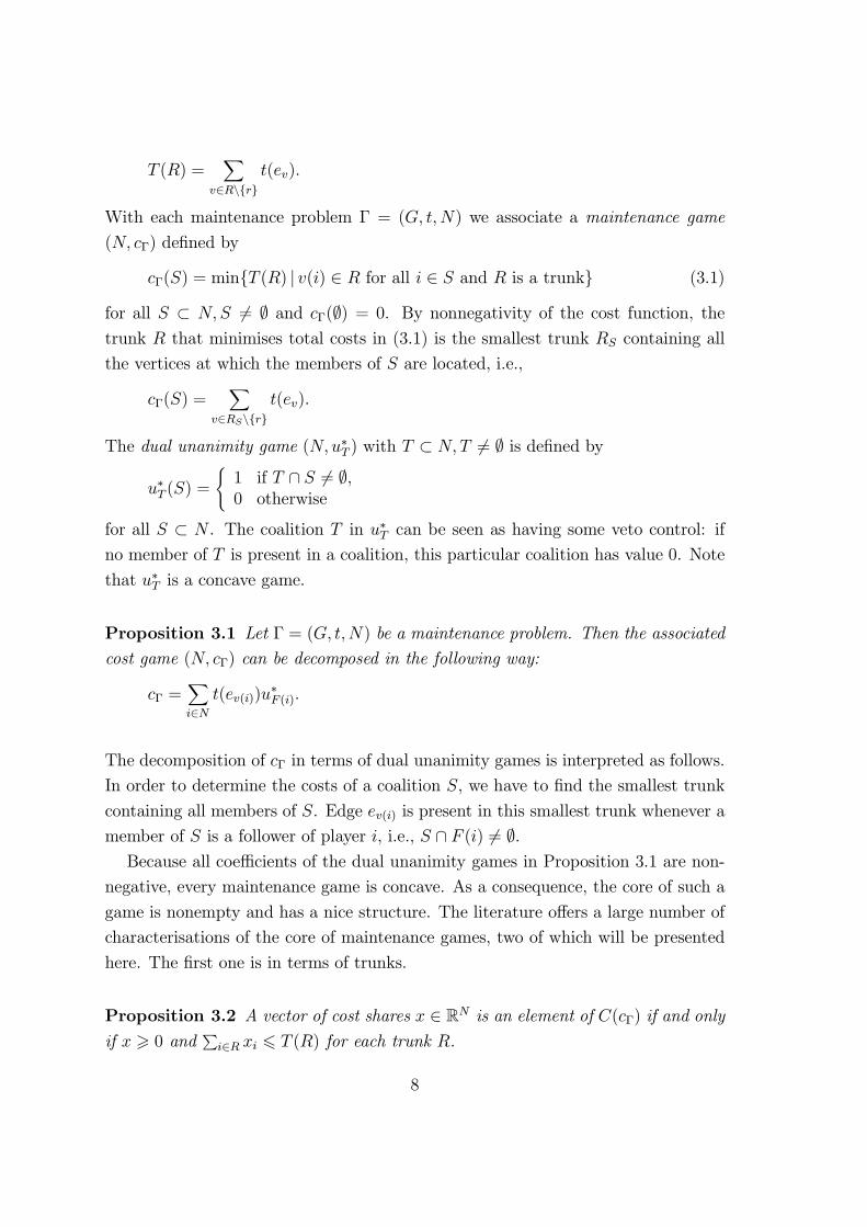
Example 3.3 Consider the mcst problem T with N = f1; 2; 3g as presented inFigure 3.3, where the numbers on the edges represent the costs.
@@
@@@¡¡¡¡¡@@
@@@¡
¡¡
¡¡tt
tt
*
1
2
3
10
6 5
12
8
10
Figure 3.3: A minimum cost spanning tree problem T
When we apply Algorithm 3.7 to this problem, the ¯rst edge we join to R is
either f¤; 1g or f¤; 3g. Suppose we choose the ¯rst one, then we set ¯R1 (T ) = 10.
Subsequently, we add f1; 2g to R, set ¯R2 (T ) = 6, add f2; 3g and set ¯R3 (T ) = 5.
This gives us a cost allocation of (10; 6; 5). On the other hand, suppose we start
with f¤; 3g. Then we end up with cost allocation ¯R(T ) = (6; 5; 10).The two minimum cost spanning trees are drawn in Figure 3.4. /
With each mcst problem T = (N; ¤; t) we associate a mcst game (N; cT ), wherecT (S) represents the minimal costs of a tree on S¤ = S [ f¤g:
cT (S) = minfX
e2Rt(e) jR ½ ES¤ and (S
¤; R) is a treeg
15

@@
@@@¡¡¡¡¡@@
@@@
tt
tt
*
1
2
3
10
6 5
¡¡¡¡¡@@
@@@¡
¡¡
¡¡tt
tt
*
1
2
3
6 5
10
Figure 3.4: Two minimum cost spanning trees
for all S ½ N;S 6= ; and cT (;) = 0. The following theorem comes from Granot and
Huberman (1981).
Theorem 3.8 Let T = (N; ¤; t) be a minimum cost spanning tree problem. Then
for every minimum cost spanning tree (N¤; R), Bird's allocation rule ¯R(T ) is anextreme point of the core of the corresponding minimum cost spanning tree game
(N; cT ).
It immediately follows that every mcst is balanced. An alternative proof for
nonemptiness of the core is given in Granot and Huberman (1982).
A further overview of mcst problems is given in Aarts (1994) and the core and
nucleolus are studied in Granot and Huberman (1984) and Solymosi et al. (1998).
Aarts and Driessen (1993) study the irreducible core of mcst games, which is a
subset of the core, and present two algorithms to determine this set. In Moretti,
Norde, Pham Do, and Tijs (2001) and Norde, Moretti, and Tijs (2001), existence of
population monotonic allocation schemes for mcst games is investigated. In Van den
Nouweland et al. (1993) it is shown that every nonnegative monotonic game arises
from an mcst problem in which there are costs associated with the vertices as well
as with the edges.
There are a large number of variations on the mcst problem as presented above. In
Feltkamp et al. (1994), minimum cost spanning extension problems are introduced,
in which there is a ¯xed tree, which has to be extended in such a way that total
extension costs are minimal. In this framework, two allocation rules are presented
that are inspired by Kruskal's algorithm for ¯nding minimum cost spanning trees. In
Suijs (2001), mcst problems are studied in which the connection costs consist of two
parts: construction costs and maintenance costs. Since the latter costs are unknown
16

ex ante, connection costs are represented by random variables. An algorithm to
determine an \optimal" network is presented and a two stage Bird allocation is
de¯ned and shown to be a core allocation of the corresponding cooperative stochastic
minimum spanning tree game (cf. Suijs (2000)).
4 Routing
In this section we discuss classes of operations research problems in which the ob-
jective is to ¯nd a route of minimal costs within a graph. First, we discuss the class
of Chinese postman games as introduced in Hamers, Borm, Van de Leensel, and
Tijs (1999). Second, we discuss travelling salesman games as introduced in Potters
et al. (1992). We discuss two variants of the travelling salesman problem: the ¯xed
routing problem and the Steiner travelling salesman problem.
In the Chinese postman problem, which is introduced in Mei-Ko Kwan (1962),
one considers a situation in which a postman has to deliver mail to each street
of a certain city. He has to start and ¯nish at the post o±ce. For each street
costs are involved each time the postman visits this street. The postman should
choose a route to visit all streets in such a way that costs are minimised. The main
di®erence between several classes of Chinese postman problems can be found in the
underlying graph that describes the street plan of the city. For the classical problem,
in which the underlying graph is undirected, Edmonds and Johnson (1973) present
a polynomially bounded matching algorithm that provides a route with minimal
costs.
A cost allocation problem arises if in the underlying graph each edge corresponds
to a di®erent player. Because all players need the mail delivery service and the
nature of this service requires the server to travel from the post o±ce and visit all
edges (players) before returning to the post o±ce, the cost allocation problem is
concerned with a fair allocation of the cost of a cheapest Chinese postman tour in
the graph. That is, the cost of a cheapest tour, which starts at the post o±ce, visits
each edge at least once and returns to the post o±ce.
Formally, a Chinese postman or CP problem is a tuple ¡ = (N;G; v0; g; t), where
N = f1; : : : ; ng is the set of players, G = (V;E) is a connected undirected graph
with vertex set V and edge set E, v0 2 V represents the post o±ce, g : E ! N
is a bijection relating the players to the edges and t : E ! R+ is a nonnegative
17

cost function assigning costs to the edges. An S-tour with respect to v0 associated
with coalition S ½ N is a closed walk (v0; e1; : : : ; ek; v0) that starts at the post
o±ce v0, visits each player in S at least once and returns to v0, i.e., S ½ fg(ej) j j 2f1; : : : ; kgg. Note that an S-tour may also use edges corresponding to players outsideS. The set of all S-tours is denoted by D(S).
Suppose a coalition S is served according to the S-tour (v0; e1; : : : ; ek; v0) 2 D(S),then the total costs of this tour are
Pkj=1 t(ej). We will assume that each player i 2 S
pays the costs t(g¡1(i)) himself. In this way we already allocate the separable costsPi2S t(g
¡1(i)) of an S-tour. Note that these separable costs are independent of
the chosen S-tour. The remaining nonseparable costs for coalition S,Pkj=1 t(ej) ¡
Pi2S t(g
¡1(i)), have to be allocated to its members in some way. This gives rise
to the Chinese postman or CP game (N; c) corresponding to ¡ = (N;G; v0; g; t),
de¯ned by
c(S) = min(v0;e1;:::;ek;v0)2D(S)
[kX
j=1
t(ej)¡X
i2St(g¡1(i))]:
for all S ½ N . In the following example, we show that a CP game need not be
balanced.
Example 4.1 Consider the CP problem (N;G; v0; g; t) with N = f1; : : : ; 5g, graphG = (V;E) as depicted in Figure 4.1, t(ej) = 1 and g(ej) = j for all j 2 f1; :::; 5g.
v
v
v
v
0
1
2
3
1 2
34
5
e e
e
e e
Figure 4.1: A Chinese postman problem
Denote the corresponding CP game by (N; c). Then c(N) = 1 and c(S) = 0 for
S 2 A = ff1; 2; 5g; f3; 4; 5g; f1; 2; 3; 4gg. Let x 2 RN and suppose x 2 C(c). Then
18
2 = 2c(N) =X
S2A
X
i2Sxi 6
X
S2Ac(S) = 0:
Contradiction, so (N; c) is not balanced. /
In spite of this result, balancedness, total balancedness and concavity have been
established for CP games that arise from some speci¯c classes of graphs. A graph
G = (V;E) is said to be globally CP balanced (totally balanced, concave) if the
induced CP game is balanced (totally balanced, concave) for all possible v0 2 V andall nonnegative cost functions on the edges. G is called locally CP balanced (totally
balanced, concave) if the induced CP game is balanced (totally balanced, concave)
for some v0 2 V and all cost functions.In Theorems 4.1 - 4.4 some results are stated from Hamers (1997), Granot et al.
(1999) and Granot and Hamers (2000).
Theorem 4.1 Let G be a connected undirected graph. Then the following three
assertions are equivalent:
(i) G is weakly Euler.
(ii) G is globally CP balanced.
(iii) G is locally CP balanced.
A graph is called weakly Euler if each biconnected component1 in G is Eulerian (i.e.,
the degree of every vertex is even).
Theorem 4.2 Let G be a connected undirected graph. Then the following ¯ve as-
sertions are equivalent:
(i) G is weakly cyclic.
(ii) G is globally CP concave.
(iii) G is globally CP totally balanced.
(iv) G is locally CP concave.
1A biconnected component of a graph G is a maximal subgraph of G in which each pair ofvertices is connected by at least two edge disjoint paths.
19

(v) G is locally CP totally balanced.
A graph G is called weakly cyclic if each biconnected component is a circuit.
The Chinese postman problem in which the underlying graph is directed has also
been studied in the literature. All de¯nitions for the undirected case as presented
above can be extended to the directed case in a straightforward way.
Theorem 4.3 Let G be a strongly connected directed graph. Then G is globally CP
balanced.
The proof of Theorem 4.3 translates the problem to a linear programming problem
and applies a balancedness result established in Owen (1975).
Theorem 4.4 Let G be a strongly connected directed graph. Then G is directed
weakly cyclic if and only if G is globally CP concave.
A directed weakly cyclic graph is a 1-sum2 of directed circuits.
We conclude the discussion on CP games by considering an allocation rule for
the class of problems in which the underlying graph is an undirected weakly Euler
graph. This class of CP problems with player set N is denoted by WEN .
In order to introduce a rule that divides for each ¡ = (N;G; v0; g; t) 2 WEN thecosts of a minimal N -tour among the players, we need the notion of followers of a
bridge with respect to v0. An edge of G is called a bridge if removal of this edge
leads to a disconnected graph. We denote the set of bridges in G by B(G). Edge
e 2 E is called a follower of b with respect to v0 if each path that contains both v0and e also contains b. The set of followers of b will be denoted by Fb(G; v0). Note
that b 2 Fb(G; v0) and that the set of followers depends on the location of v0 in thegraph.
Let b 2 B(G). Then the postman needs to cross this bridge twice if he is to
make a tour containing some edge in Fb(G; v0). It seems reasonable that each player
in Fb(G; v0) will pay an equal share of the costs of crossing b for the second time.
So, if a tour that visits a certain player contains bridges, he has to contribute a
2The 1-sum of graphs G and H is de¯ned as the graph derived from G and H by coalescingone vertex in G with another vertex in H.
20
fair share in the nonseparable costs of all these bridges. Formally, the division rule
° :WEN ! RN is de¯ned for all ¡ = (N;G; v0; g; t) 2 WEN by
°g(e)(¡) =X
b2B(G):e2Fb(G;v0)
t(b)
jFb(G; v0)j
for all e 2 E.The following example illustrates the ° rule.
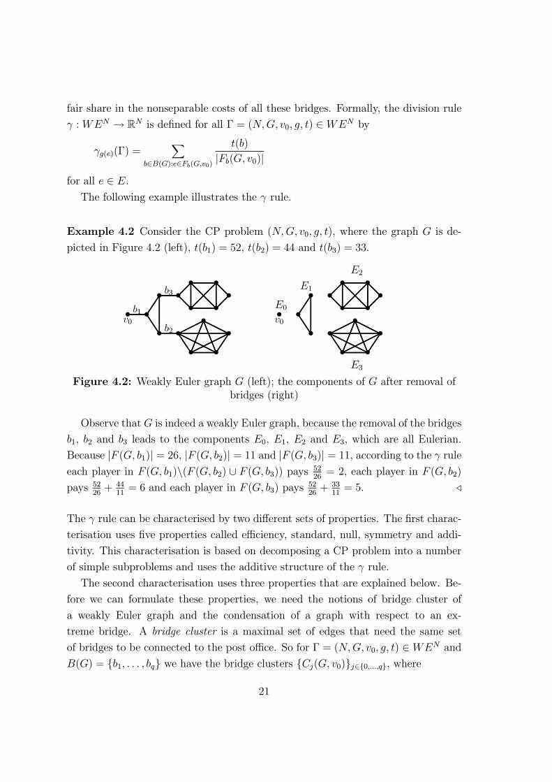
Example 4.2 Consider the CP problem (N;G; v0; g; t), where the graph G is de-
picted in Figure 4.2 (left), t(b1) = 52, t(b2) = 44 and t(b3) = 33.
..................................................................................................................................................................................................................................................................................................................................................................................................................................
......................................................................................................................................................................................................................................................................................................................................................................................................................................................................................................................................................................................................................................................................................
................
................
................
................
................
.....................................................................
..................................................................................................................................................................................................................................................................................................................................................................................................
................
................
................
................
.....
................
................
................
................
.....
..................................................................................................................................................................................................
v0b1
b2
b3
² ²² ²
² ²²
²
² ²² ²
²²²
.............................................................. ............................................................................................................................................................................................................................................................
......................................................................................................................................................................................................................................................................................................................................................................................................................................................................................................................................................................................................................................................................................
................
................
................
................
................
.....................................................................
..............................................................................................................................................................................................................................................................................................................................................
................
................
................
................
.....
................
................
................
................
.....
..................................................................................................................................................................................................
v0
E0
E1
E2
E3
² ²² ²
² ²²
²
² ²² ²
²²²
Figure 4.2: Weakly Euler graph G (left); the components of G after removal ofbridges (right)
Observe thatG is indeed a weakly Euler graph, because the removal of the bridges
b1, b2 and b3 leads to the components E0, E1, E2 and E3, which are all Eulerian.
Because jF (G; b1)j = 26, jF (G; b2)j = 11 and jF (G; b3)j = 11, according to the ° ruleeach player in F (G; b1)n(F (G; b2) [ F (G; b3)) pays 52
26= 2, each player in F (G; b2)
pays 5226+ 44
11= 6 and each player in F (G; b3) pays
5226+ 33
11= 5. /
The ° rule can be characterised by two di®erent sets of properties. The ¯rst charac-
terisation uses ¯ve properties called e±ciency, standard, null, symmetry and addi-
tivity. This characterisation is based on decomposing a CP problem into a number
of simple subproblems and uses the additive structure of the ° rule.
The second characterisation uses three properties that are explained below. Be-
fore we can formulate these properties, we need the notions of bridge cluster of
a weakly Euler graph and the condensation of a graph with respect to an ex-
treme bridge. A bridge cluster is a maximal set of edges that need the same set
of bridges to be connected to the post o±ce. So for ¡ = (N;G; v0; g; t) 2 WEN andB(G) = fb1; : : : ; bqg we have the bridge clusters fCj(G; v0)gj2f0;:::;qg, where
21

C0(G; v0) = En [b2B(G) Fb(G; v0)
is the set of edges that do not need any bridge to be connected to v0 and for all
j 2 f1; : : : ; qg
Cj(G; v0) = Fbj (G; v0)n [b2B(G)\Fbj (G;v0);b 6=bj Fb(G; v0)
is the cluster of edges that need the bridges fb 2 B(G) j bj 2 Fb(G; v0)g to beconnected to v0. A bridge bj 2 B(G) is called an extreme bridge of G if it has no
other bridge as a follower, or equivalently, if Cj(G; v0) = Fbj (G; v0). The following
example illustrates the notions of bridge cluster and extreme bridge.
Example 4.3 Consider the graph G in Example 4.2. Then C0(G; v0) = E0 and
Cj(G; v0) = Ej [ fbjg for j 2 f1; 2; 3g. The extreme bridges are b2 and b3. /
Next, we describe a procedure to construct the condensed graph of a weakly Euler
graph G with respect to an extreme bridge. Let v0 2 V and let b 2 B(G) be an
extreme bridge of G. Let v¤1 be incident on b such that there exists a path between
v0 and v¤1 in the graph (V;Enfbg). Let V (Fb(G; v0)) be the set of vertices incident on
the edges in Fb(G; v0). The graph G arises from G by removing all edges Fb(G; v0)
and vertices V (Fb(G; v0))nfv¤1g. Let jFb(G; v0)j = m, then the graph G¤ arises fromG by connecting a circuit of length m to the vertex v¤1. The graph G
¤ is called the
condensed graph of G with respect to the extreme bridge b. Note that G¤ is also a
weakly Euler graph. Moreover, the number of edges in G and G¤ coincide.
Example 4.4 Consider the graph G in Example 4.2. Figure 4.3 shows the graph
G¤ that arises from G by condensation with respect to the extreme bridge b3. /
The condensed CP problem of ¡ = (N;G; v0; t; g) 2 WEN with respect to the
extreme bridge b 2 B(G) is ¡b = (N;G¤; v0; t¤; g¤), where G¤ = (V ¤; E¤) is the
condensed graph of G with respect to b, g¤ : E¤ ! N is a bijection such that
g¤(e) = g(e) for all e 2 EnFb(G; v0) and the cost function t¤ : E¤ ! R+ is de¯ned
by
t¤(e) =
(t(e) if e 2 EnFb(G; v0);0 otherwise:
Let ¡ = (N;G; v0; g; t) 2 WEN . Consider the following three properties for a
division rule f : WEN ! RN :
22

...............................................................................................................................................................................................................................................................................................................................................................................................................................................................................................
.................................................................................................................................................................................................................................................................................................................................................................................................................................................................................................................................................................................................................................................................................................................................................................................................................................................................................................
................
................
................
................
................
................
................
..............................................................................
.................................................................................................................................................................................................................................................................................................................................................................................................................................................................................................
................
................
................
................
................
......
................
................
................
................
................
......
..................................................................................................................................................................................................................................................
...............................................................................................................................................................................................................................................................................................................................................................................................................................................................................................
.................................................................................................................................................................................................................................................................................................................................................................................................................................................................................................................................................................................................................................................................................................................................................................................................................................................................................................
................
................
................
................
................
................
................
..............................................................................
.......................................................................................................................................................................................................................................................................................................................................................................................................................................................................................................................................................
..............................................................
v0 v1
v2 v3
v4 v5
v6
v7
v¤1b3
v9
v10 v11
v12
v13v14
² ²
² ²
² ²
²²
² ²² ²
²²²
v0 v1
v2 v3
v4 v5
v6
v7
v¤1
v¤2v¤3 v¤4
v¤5v¤6v¤7v¤8
v¤9v¤10v¤11
² ²
² ²
² ²
²²
²² ² ² ²
²²
²²²² ²
Figure 4.3: The condensed graph G¤ from G with respect to b3
² E±ciency: Pi2N fi(¡) =
Pb2B(G) t(b).
² Bridge cluster symmetry: Let B(G) = fb1; : : : ; bqg, then fg(e1)(¡) = fg(e2)(¡)for all e1; e2 2 Cj(G; v0), j 2 f0; : : : ; qg.
² Condensation property: Let b be an extreme bridge of G and let ¡b =
(N;G¤; v0; g¤; t¤) be the condensed problem with respect to b, then fg(e)(¡) =
fg(e)(¡b) for all e 2 EnFb(G; v0).
Bridge cluster symmetry states that each group of players that need the same set
of bridges to be connected to the post o±ce will contribute the same share in the
nonseparable costs. The condensation property is a kind of consistency property.
All players who are not in the bridge cluster corresponding to the removed bridge
face the same problem in this reduced graph as in the original graph. Now, a rule is
called consistent if in both situations this rule assigns to each player in this group
the same costs.
Theorem 4.5 The allocation rule ° : WEN ! RN is the unique rule that satis¯es
e±ciency, bridge cluster symmetry and the condensation property.
Whereas in the Chinese postman problem each edge in the graph has to be visited
at least once, in the travelling salesman problem one aims to ¯nd a tour that visits
all the vertices in the graph exactly once. For example, a professor has to make a
trip visiting several universities. He has to start at his own university, visit all other
universities exactly once and then return to his home university. The problem is
23

to select a route in which total travel costs are minimised. It is well known that
¯nding such a route is an NP-hard problem. Nevertheless, many real life problems
are related to the travelling salesman problem. This has resulted in many heuristic
approaches to ¯nd good solutions to several variants of this problem. For a review
on the travelling salesman problem we refer to Lawler et al. (1985).
Fishburn and Pollack (1983) introduce the cost allocation problem that arises if
in the underlying graph each vertex, except the one that corresponds to the home
location, corresponds to a di®erent player. The cost allocation is concerned with a
fair allocation of the cost of a cheapest Hamiltonian circuit in the graph. That is
the cheapest tour that starts in the vertex that corresponds to the home location,
visits all other vertices precisely once and returns home.
Formally, a travelling salesman or TS problem is a tuple (N; ¤; t), where N =
f1; : : : ; ng is the set of players, ¤ represents the home location and t : EN¤ ! R+ is
the cost function assigning costs to the edges connecting the vertices inN¤ = N[f¤g.We assume that t satis¯es the triangle inequality. ES is de¯ned as the set of all edges
between pairs of elements of S, so that (S;ES) is the complete graph on S:
ES = ffi; jg j i; j 2 S; i 6= jg:
By de¯ning the worth of a coalition S as the minimal costs of a Hamiltonian circuit
in the graph (S [ f¤g; ES[f¤g), we obtain the corresponding travelling salesman orTS game.
The following example, due to Tamir (1989), illustrates that TS games need not
be balanced.
Example 4.5 Consider the TS problem (N; ¤; t) with player set N = f1; : : : ; 6g,t(fi; jg) = 1 for all edges fi; jg depicted in Figure 4.4 and for all other edges fi; jg,t(fi; jg) equals the minimal costs of a path connecting i to j using the depictededges.
We denote the corresponding TS game by (N; c). Then c(N) = 8 (with optimal
tour (¤; 4; 5; 6; 1; 2; 3; ¤)), c(f1; 2; 4; 5g) = 5, c(f3; 4; 5; 6g) = 5 and c(f1; 2; 3; 6g) = 5.Let x 2 RN and suppose x 2 C(c), then
16 = 2c(N) =X
i2f1;2;4;5gxi +
X
i2f3;4;5;6gxi +
X
i2f1;2;3;6gxi 6 5 + 5 + 5 = 15:
Contradiction, so (N; c) is not balanced. /
24

1
234
5
6
*
Figure 4.4: A travelling salesman problem
In case there are less than six players some results with respect to balancedness are
established. Potters et al. (1992) show that 3-person TS games have a nonempty
core. Tamir (1989) shows that each 4-person TS game has a nonempty core and
provides Example 4.5 showing that a 6-person TS game can have an empty core.
Finally, Kuipers (1993) proves that 5-person TS games are balanced.
The travelling salesman model can be extended to the case in which the costs
depend on the direction in which the salesman travels through the edges. In this
context, Potters et al. (1992) provide a 4-person TS game with an empty core.
Potters et al. (1992) also introduce the class of ¯xed routing games. The idea of a
¯xed routing game is that the salesman decides about the Hamiltonian circuit he will
use to visit all the players. Then the value of a coalition S in a ¯xed routing game
is de¯ned as the costs of the restricted tour that visits the players in S in the same
order as prescribed by the original Hamiltonian circuit and skips all other players.
Potters et al. (1992) show that ¯xed routing games have a nonempty core if the
chosen Hamiltonian circuit is an optimal route for the related TS problem. Derks
and Kuipers (1997) give a time e±cient algorithm that calculates core elements of
¯xed routing games. In Kuipers et al. (2000) and Solymosi et al. (1998) O(n4)algorithms are provided that calculate the nucleolus of ¯xed routing games.
Finally, we mention Steiner TS games. These games arise from situations in
which some of the edges between pairs of players may be absent. The value of a
coalition in a Steiner TS game corresponds to the costs of the cheapest Steiner tour.
A Steiner tour is a closed trail that starts in the home location and visits each vertex
of S at least once. For these games Herer and Penn (1995), Granot et al. (2000)
25

and Granot and Hamers (2000) have characterised concavity by the structure of the
available edges.
5 Scheduling
In this section we discuss classes of operations research games that are related to
scheduling problems. First, we discuss various classes of sequencing games as initi-
ated by Curiel et al. (1989). We focus on balancedness and convexity and discuss
two context speci¯c solution concepts: the equal gain splitting rule and the split
core. Second, we consider permutation games, introduced in Tijs et al. (1984),
where we focus on total balancedness. Finally, we discuss assignment games, in-
troduced in Shapley and Shubik (1971), which form a special class of permutation
games and have some appealing properties with respect to the structure of the core.
The main characteristic of a sequencing situation is that a number of jobs (tasks,
operations) have to be processed in some order on a (number of) machine(s) in such
a way that some cost criterion is minimised. In spite of this common characteristic,
sequencing situations can be classi¯ed on the basis of many features. We mention
the number of machines, the speci¯c properties of machines (e.g., parallel, serial),
the chosen cost criterion (e.g., maximum completion time, weighted completion
time), restrictions on the jobs (e.g., ready times, due dates) and possibly the speci¯c
order in which the jobs have to be processed on the machines (e.g., job-shop, °ow-
job). Obviously, sequencing situations arise in many applications: the process of
manufacturing cars, allocating patients to surgery rooms, maintenance of airplanes,
etc. For a review of scheduling theory we recommend Lawler et al. (1993).
As a speci¯c example we describe the class of one-machine sequencing situations
as introduced in Curiel et al. (1989). In a one-machine sequencing situation there is a
queue of players, each with one job, in front of a machine. Each player must have his
job processed on this machine. The ¯nite set of players is denoted by N = f1; :::; ng.The positions of the players in the queue are described by a bijection ¾ 2 ¦N . Weassume that there is an initial order ¾0 2 ¦N on the jobs before the processing ofthe machine starts. The processing time pi of the job of player i is the time the
machine takes to handle this job. For each player i 2 N the costs of spending time
in the system can be described by a linear cost function ci : R+ ! R de¯ned by
ci(t) = ®it with ®i > 0: A sequencing situation as described above is denoted by
26

(N; ¾0; p; ®) with p; ® 2 RN++.
The completion time C(¾; i) of the job of player i if the jobs are processed (in a
semi-active way) according to the order ¾ 2 ¦N is given byC(¾; i) =
X
fj2N j¾(j)6¾(i)gpj :
A processing order is called semi-active if there does not exist a job which could be
processed earlier without altering the processing order, i.e., if there are no unneces-
sary delays. The total costs of all players if the jobs are processed according to the
order ¾ equalPi2N ®iC(¾; i). Clearly, because ¦N is ¯nite, there exists an order
for which total costs are minimised. A processing order that minimises total costs
and thus maximises total cost savings is an order in which the jobs are processed in
decreasing order with respect to the urgency index ui de¯ned by ui =®ipi(cf. Smith
(1956)).
Example 5.1 Consider a one-machine sequencing situation (N;¾0; p; ®), where
N = f1; 2; 3g, ¾0 = (1; 2; 3), p = (2; 2; 1) and ® = (4; 6; 5). Then the urgencies
for the players are u1 = 2, u2 = 3 and u3 = 5, respectively. Hence, the optimal
processing order is (3; 2; 1) with total costs 5 ¢ 1 + 6 ¢ 3 + 4 ¢ 5 = 43. /
Note that an optimal order can be obtained from the initial order by consecutive
switches of neighbours i; j with i directly in front of j and ui < uj . This process
will be referred to as the Smith algorithm.
By rearranging from the initial order to an optimal order, an allocation problem
arises: how should the maximal total cost savings the players can obtain be divided
among the players? Again, this problem is tackled using cooperative game theory
by analysing corresponding sequencing games.
For a sequencing situation (N; ¾0; p; ®) the costs CS(¾) of coalition S with respect
to a processing order ¾ equal CS(¾) =Pi2S ®iC(¾; i). We want to determine the
maximal cost savings of a coalition S when its members decide to cooperate. For
this, we have to de¯ne which rearrangements of the coalition S are admissible with
respect to the initial order. A bijection ¾ 2 ¦N is called admissible for S if it satis¯esthe following condition:
P (¾; j) = P (¾0; j)
for all j 2 NnS, where for any ¿ 2 ¦N the set of predecessors of a player j 2 N
with respect to ¿ is de¯ned as P (¿; j) = fk 2 N j ¿(k) < ¿ (j)g.
27

This condition implies, in particular, that the starting time of each player outside
the coalition S is equal to his starting time in the initial order and the players of S
are not allowed to \jump" over players outside S. The set of admissible orders for
a coalition S is denoted by A(S).By de¯ning the value of a coalition S as the maximum cost savings coalition S
can achieve by means of an admissible rearrangement we obtain the corresponding
sequencing game (N; v), which is de¯ned by
v(S) = max¾2A(S)
fX
i2S®i[C(¾0; i)¡ C(¾; i)]g (5.1)
for all S ½ N .
Expression (5.1) can be rewritten in terms of gij = maxf0; ®jpi ¡ ®ipjg, whichequals the cost savings attainable by player i and j when i is directly in front of
j, regardless of the exact position in the order. For this we need the notion of
connected coalition. A coalition S is called connected with respect to ¾ if for all
i; j 2 S and k 2 N such that ¾(i) < ¾(k) < ¾(j) it holds that k 2 S. The Smithalgorithm and (5.1) imply the following proposition.
Proposition 5.1 Let (N;¾0; p; ®) be a sequencing situation and let (N; v) be the
corresponding sequencing game. Then for any coalition S that is connected with
respect to ¾0 we have
v(S) =X
i;j2S:¾0(i)<¾0(j)gij :
For a coalition T that is not connected with respect to ¾0 the de¯nition of admissible
orders implies that
v(T ) =X
S2Tn¾0v(S);
where Tn¾0 is the set of components of T , a component of T being a maximallyconnected subset of T .
Example 5.2 Let N = f1; 2; 3g, ¾0 = (1; 2; 3), p = (2; 2; 1) and ® = (4; 6; 5). It
is readily veri¯ed that g12 = g23 = 4 and g13 = 6. Then v(fig) = 0 for all i 2 N ,v(f1; 2g) = v(f2; 3g) = 4, v(f1; 3g) = v(f1g) + v(f3g) = 0 and v(N) = 14. /
28

The following theorem, due to Curiel et al. (1989), shows that sequencing games
are convex games.
Theorem 5.2 Let (N;¾0; ®; p) be a sequencing situation. Then the corresponding
sequencing game (N; v) is convex.
In particular, Theorem 5.2 implies that sequencing games are (totally) balanced.
Another way of proving balancedness of sequencing games is by explicitly con-
structing core allocations. We will show that the the equal gain splitting rule,
introduced in Curiel et al. (1989), and the split core, introduced in Hamers et al.
(1996), are rules that yield allocations that are in the core of the corresponding
sequencing games.
Recall that the set of predecessors of player i 2 N with respect to the processing
order ¾ is given by P (¾; i) = fj 2 N j ¾(j) < ¾(i)g: We de¯ne the set of followersof i 2 N with respect to ¾ to be F (¾; i) = fj 2 N j ¾(j) > ¾(i)g. The equal gainsplitting or EGS rule is a map that assigns to each sequencing situation (N;¾0; p; ®)
a vector in RN , which is de¯ned by
EGSi(N; ¾0; p; ®) =1
2
X
j2F (¾0;i)gij +
1
2
X
k2P (¾0;i)gki (5.2)
for all i 2 N . Equation (5.2) means that the EGS rule assigns to each player halfof the gains of all neighbour switches he is actually involved in when reaching an
optimal order from the initial order.
From (5.2) it readily follows that the EGS rule is e±cient, i.e.,X
i2NEGSi(N; ¾0; p; ®) =
X
i;j2N :¾0(i)<¾0(j)gij = v(N):
Example 5.3 Let N = f1; 2; 3g, ¾0 = (1; 2; 3), p = (2; 2; 1) and ® = (4; 6; 5).
Because g12 = g23 = 4 and g13 = 6 we have EGS1(N;¾0; p; ®) =12(4 + 6) = 5,
EGS2(N; ¾0; p; ®) =12(4 + 4) = 4 and EGS3(N;¾0; p; ®) =
12(6 + 4) = 5. Moreover,
we havePi2N EGSi(N; ¾0; p; ®) = 4 + 4 + 6 = 14 = v(N). /
A nice feature of the EGS rule is that it can be characterised using three appealing
properties. Let SEQN denote the class of one-machine sequencing situations with
player set N . Consider the following properties for a rule f : SEQN ! RN+ with
(N; ¾0; p; ®) 2 SEQN :
29

² E±ciency: Let ¼ be an optimal processing order for N . Then f is callede±cient if
Pi2N fi(N;¾0; p; ®) = CN(¾0)¡ CN(¼).
² Equivalence property: Let i 2 N and (N; ¾1; p; ®) 2 SEQN be such
that P (¾0; i) = P (¾1; i). Then f satis¯es the equivalence property if
fi(N; ¾0; p; ®) = fi(N; ¾1; p; ®).
² Switch property: Let i; j 2 N be such that j¾0(i) ¡ ¾0(j)j = 1. Let
(N; ¾1; p; ®) 2 SEQN be such that ¾1(i) = ¾0(j) , ¾1(j) = ¾0(i) and
¾1(k) = ¾0(k) for all k 2 Nnfi; jg. Then f satis¯es the switch property iffi(N; ¾0; p; ®)¡ fi(N; ¾1; p; ®) = fj(N; ¾0; p; ®)¡ fj(N; ¾1; p; ®).
The equivalence property states that the order of a player's predecessors does not
a®ect his allocation. For explaining the switch property, let two players be neigh-
bours in a sequencing situation. If these players switch positions, then the switch
property states that in this new situation the allocation is increased (or decreased)
equally for both players. These three properties characterise the EGS rule.
Theorem 5.3 The EGS rule is the unique rule on SEQN that satis¯es e±ciency,
the equivalence property and the switch property.
The proof of Theorem 5.3 is one by induction on the number of misplacements. A
pair fi; jg is called a misplacement in an order ¾ if they are neighbours in ¾ and theurgency of the player in front is smaller than the urgency of its neighbour.
Generalising the EGS rule, we consider gain splitting (GS) rules in which each
player obtains a nonnegative part of the gain of all neighbour switches he is involved
in to reach the optimal order. Again, the total gain of a neighbour switch is only
divided among the two players that are involved. Formally, we de¯ne for all i 2 Nand all ¸ 2 ¤
GS¸i (N; ¾0; p; ®) =X
j2F (¾0;i)¸ijgij +
X
k2P (¾0;i)(1¡ ¸ki)gki;
where ¤ = ff¸ijgi;j2N;¾0(i)<¾0(j) j 8i;j2N;¾0(i)<¾0(j) : 0 6 ¸ij 6 1g. Note that
GS¸(N; ¾0; p; ®) = EGS(N;¾0; p; ®) in case every ¸ij equals12.
Example 5.4 If we take ¸12 =34, ¸13 =
13and ¸23 = 1 in the sequencing situation
of Example 5.3, then GS¸(N;¾0; p; ®) = (5; 5; 4). /
30

The split core of a sequencing situation (N;¾0; p; ®) is de¯ned by
SPC(N; ¾0; p; ®) = fGS¸(N;¾0; p; ®) j ¸ 2 ¤g:
The split core can be characterised using similar properties as in the characterisation
of the EGS rule. Finally, we state that the EGS rule and the split core generate
core allocations for sequencing games.
Theorem 5.4 Let (N; ¾0; p; ®) 2 SEQN and let (N; v) be the corresponding se-
quencing game. Then SPC(N; ¾0; p; ®) ½ C(v).
Yet another proof for balancedness is provided in Curiel et al. (1995). They intro-
duce the class of component additive games, which contains the class of sequencing
games, and prove that the average of two speci¯c marginal vectors, the ¯ rule, lies
in the core of such a game. In fact, it turns out that the ¯ rule coincides with the
EGS rule within the class of sequencing games.
In the literature many other classes of sequencing games are studied. Hamers
et al. (1995) extend the class of one-machine sequencing situations considered by
Curiel et al. (1989) by imposing ready times on the jobs. In this case the corre-
sponding sequencing games are balanced, but not necessarily convex. For a special
subclass of sequencing games with ready times, however, convexity can be estab-
lished. Borm et al. (1999) consider some classes of sequencing situations in which
due dates are imposed on the jobs and di®erent cost criteria are used: weighted com-
pletion time, weighted tardiness and weighted penalty. Several convexity results are
established.
Instead of imposing restrictions on the jobs, Hamers, Klijn, and Suijs (1999),
Calleja et al. (2001) and Van den Nouweland et al. (1992) extend the number of
machines. Hamers, Klijn, and Suijs (1999) consider sequencing situations with m
parallel and identical machines in which no restrictions on the jobs are imposed.
Again, the weighted completion time criterion is used. Balancedness is established
for two-machine situations by showing that these games are component additive
games. In case there are more than two machines, balancedness is shown for two
special classes. Calleja et al. (2001) establish balancedness for a special class of
sequencing games that arise from two-machine sequencing situations in which a
maximal weighted cost criterion is considered. Van den Nouweland et al. (1992)
consider multiple machine °ow-shop sequencing situation with a dominant machine.
31
Convexity is established in case the ¯rst machine is the dominant machine by show-
ing that this class of games coincides with the class of sequencing games discussed
in Curiel et al. (1989). In case another machine is the dominant machine, the
corresponding game need not be balanced.
Van Velzen and Hamers (2001) consider some classes of sequencing games that
arise from relaxations of classical sequencing situations. By allowing more admis-
sible rearrangements, coalitions have more possibilities to maximise their pro¯t.
Balancedness is shown for some of these classes. Other related papers in the ¯eld of
sequencing games are Curiel et al. (1994), Hamers (1995), Suijs et al. (1997) and
Curiel et al. (1997).
Permutation games, introduced by Tijs et al. (1984), arise from situations in which
every player has one job and one machine. Every job has to be processed on a
machine and each machine can process every job, but no machine is allowed to
process more than one job. If player i processes his job on the machine of player
j, the processing costs are aij . Let N = f1; : : : ; ng be the set of players. Thecorresponding permutation game (N; v) is the cooperative game de¯ned by
v(S) =X
i2Saii ¡ min
¼2¦S
X
i2Sai¼(i)
for all S ½ N;S 6= ; and v(;) = 0. The number v(S) denotes the maximal cost
savings a coalition S can obtain by processing their jobs according to an optimal
schedule compared to the situation in which every player processes his job on his
own machine. The following example illustrates that a permutation game need not
be convex.
Example 5.5 Let N = f1; 2; 3g be the player set and let
A =
0B@8 4 22 4 105 6 10
1CA
be the cost matrix. Then the corresponding permutation game (N; v) is given by:
S f1g f2g f3g f1; 2g f1; 3g f2; 3g f1; 2; 3gv(S) 0 0 0 6 11 0 12
E.g., the optimal schedule for the grand coalition is to process player 1's job on
machine 3, player 2's job on machine 1 and player 3's job on machine 2, giving total
cost savings of 8+4+10-(2+2+6)=12.
32

For this game we have
v(f1; 2; 3g)¡ v(f1; 3g) = 1 < 6 = v(f1; 2g)¡ v(f1g);
which implies that (N; v) is not convex. /
It can be shown that the core of a permutation game is nonempty. Since every
subgame of a permutation game is again a permutation game, we have the following
result.
Theorem 5.5 Permutation games are totally balanced.
For Theorem 5.5 several proofs are presented in the literature. We mention Tijs
et al. (1984), using the Birkho®-Von Neumann theorem on doubly stochastic ma-
trices. Curiel and Tijs (1986) use an equilibrium existence theorem of Gale (1984)
for a discrete exchange economy with money. Klijn et al. (2000) use the existence
of envy-free allocations in speci¯c economies with indivisible objects and money to
prove balancedness of permutation games.
An interesting subclass of permutation games is the class of assignment games,
introduced in Shapley and Shubik (1971). These games are inspired on two-sided
markets in which indivisible objects are exchanged for money. Applications that
can be analysed using assignment games are, e.g., private markets in used cars, real
estate markets and auctions.
Formally, assignment games arise from bipartite matching situations. LetM and
N be two ¯nite, disjoint sets. For each i 2 M and j 2 N the monetary value of a
matching between i and j is given by aij > 0. Corresponding to this situation an
assignment game is de¯ned in the following way. On the player setM [N , the valueof the coalition S [ T , S ½ M;T ½ N is de¯ned to be the maximum that S [ Tcan obtain by making matchings between players in S and T . If S = ; or T = ; nosuitable pairs can be made and therefore the value of such a coalition equals 0.
The following example illustrates that an assignment game need not be convex.
Example 5.6 Let M = f1; 2g and N = f3; 4g. Let a13 = 3, a14 = 5, a23 = 1 anda24 = 4. The coalitions with nonzero value in the corresponding assignment game
(N; v) are presented in the following table:
33

S f1; 3g f1; 4g f2; 3g f2; 4gv(S) 3 5 1 4
S f1; 2; 3g f1; 2; 4g f1; 3; 4g f2; 3; 4g f1; 2; 3; 4gv(S) 3 5 5 4 7
E.g., the optimal assignment for the grand coalition consists of a matching between
players 1 and 3 and a matching between players 2 and 4.
For this game we have
v(f1; 2; 3; 4g)¡ v(f1; 2; 4g) = 2 < 3 = v(f1; 3g)¡ v(f1g);
which implies that (N; v) is not convex. /
Every assignment game is a permutation game. Let A = (aij)i2M;j2N denote a
matrix with corresponding assignment game (M [N; v), then the jM [N j£jM [N jmatrix
"0 ¡A0 0
#
gives rise to a permutation game, which equals v. Hence, it follows from Theorem 5.5
that assignment games are totally balanced.
In contrast to permutation games, the structure of the core of assignment games
has been studied extensively. Shapley and Shubik (1971) show that the set of core
allocations coincides with the set of solutions of the linear programming problem
that is the dual of the optimal assignment problem. Moreover, they observe that the
core corresponds to the set of competitive price equilibria of an economy associated
with the assignment problem (cf. Debreu and Scarf (1963)). Shapley and Shubik
(1971) also prove that the core expressed as a set of utility vectors for the players
in M (or N) is a lattice. It is easy to see that the lattice is of a special type called
the \45±-lattice". Quint (1991a) shows that also the converse is true, i.e., that every
45±-lattice can be associated with the core of an appropriately de¯ned assignment
game. Balinsky and Gale (1990) show that the number of extreme points of the
core cannot exceed
Ã2kk
!, where k = minfjM j; jN jg. More recently, Hamers,
Klijn, Solymosi, Tijs, and Villar (1999) have shown that the core of an assignment
game satis¯es the CoMa property, i.e., the core is the convex hull of some marginal
vectors. Nu~nez and Rafels (2000) relate the extreme points of the core to reduced
marginal vectors. Solymosi and Raghavan (1994) present an O(n4) algorithm to ¯nd
34
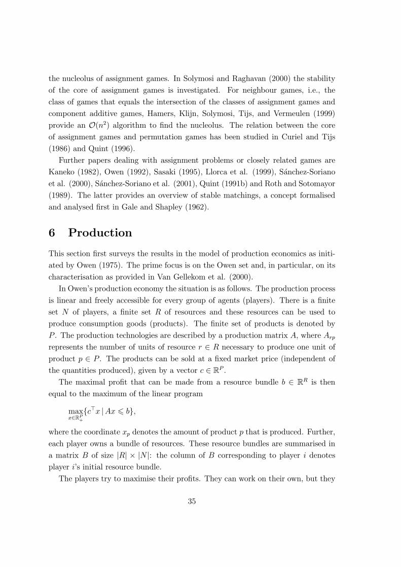
the nucleolus of assignment games. In Solymosi and Raghavan (2000) the stability
of the core of assignment games is investigated. For neighbour games, i.e., the
class of games that equals the intersection of the classes of assignment games and
component additive games, Hamers, Klijn, Solymosi, Tijs, and Vermeulen (1999)
provide an O(n2) algorithm to ¯nd the nucleolus. The relation between the core
of assignment games and permutation games has been studied in Curiel and Tijs
(1986) and Quint (1996).
Further papers dealing with assignment problems or closely related games are
Kaneko (1982), Owen (1992), Sasaki (1995), Llorca et al. (1999), S¶anchez-Soriano
et al. (2000), S¶anchez-Soriano et al. (2001), Quint (1991b) and Roth and Sotomayor
(1989). The latter provides an overview of stable matchings, a concept formalised
and analysed ¯rst in Gale and Shapley (1962).
6 Production
This section ¯rst surveys the results in the model of production economics as initi-
ated by Owen (1975). The prime focus is on the Owen set and, in particular, on its
characterisation as provided in Van Gellekom et al. (2000).
In Owen's production economy the situation is as follows. The production process
is linear and freely accessible for every group of agents (players). There is a ¯nite
set N of players, a ¯nite set R of resources and these resources can be used to
produce consumption goods (products). The ¯nite set of products is denoted by
P . The production technologies are described by a production matrix A, where Arp
represents the number of units of resource r 2 R necessary to produce one unit ofproduct p 2 P . The products can be sold at a ¯xed market price (independent ofthe quantities produced), given by a vector c 2 RP .
The maximal pro¯t that can be made from a resource bundle b 2 RR is then
equal to the maximum of the linear program
maxx2RP+
fc>x jAx 6 bg;
where the coordinate xp denotes the amount of product p that is produced. Further,
each player owns a bundle of resources. These resource bundles are summarised in
a matrix B of size jRj £ jN j: the column of B corresponding to player i denotes
player i's initial resource bundle.
The players try to maximise their pro¯ts. They can work on their own, but they
35
are allowed to cooperate by pooling their resources. Pooling is favourable, because
the maximal (joint) pro¯t after pooling is always at least as high as the sum of the
pro¯ts of the players separately. For, when cooperating, they could still make the
same products they make on their own. Therefore, it is assumed that all players
cooperate, yielding a maximal (total) pro¯t. The question arises how to divide this
pro¯t among the agents in a fair way. So, again, this type of situation features
not only an optimisation aspect in ¯nding an optimal production plan, but also an
allocation aspect in how to divide the corresponding pro¯ts.
A situation as described above is called an LP process and it is summarised by
L = (N;R; P;A;B; c). We make the following natural assumptions:
(i) A > 0; B > 0,
(ii) BeN > 0,
(iii) 9p2P : cp > 0,
(iv) cp > 0 ) 9r2R : Arp > 0 (no gains without input).
The class of LP processes with arbitrary but ¯nite player set satisfying (i)-(iv) is
denoted by L.To analyse the allocation problem due to cooperation, we consider associated TU
games. For L = (N;R; P;A;B; c) 2 L, the corresponding LP game vL is de¯ned by
vL(S) = maxx2F (S)
c>x
for every S ½ N , where F (S) = fx 2 RP+ jAx 6 BeSg. Note that BeS represents
the total resource bundle available to coalition S and vL(S) is the maximal pro¯t
the players in S can jointly generate by pooling their resources.
From duality theory we know that
vL(S) = miny2F ¤
y>BeS
with F ¤ = fy 2 RR+ j y>A > c>g, since it is readily checked that the feasible regions
F (S) and F ¤ are both nonempty.
It is important to note that the feasible region F ¤ of the dual program does
not depend on the coalition S one is considering and hence can be readily used to
determine vL just by changing the objective function.
36

Example 6.1 Consider the LP process L with N = f1; 2; 3g, two resources andtwo products:
A =
"2 11 4
#; B =
"28 42 028 0 35
#and c> =
h6 8
i:
The dual feasible region F ¤ (for any coalition) is given by
2y1 + y2 > 6; y1 + 4y2 > 8; y1 > 0; y2 > 0:
From this we readily derive (e.g., by comparing the value of the objective function
in the corner points) that the corresponding LP game vL is given by
S ; f1g f2g f3g f1; 2g f1; 3g f2; 3g f1; 2; 3gvL(S) 0 104 0 0 168 154 146 250
Note that (BeN)> =h70 63
iand miny2F¤ y>BeN = 250 is (uniquely) attained
in (167; 107), while for S = f1; 2g, (BeS)> =
h70 28
iand miny2F ¤ y>BeS = 168 is
attained in (0; 6). /
For L = (N;R; P;A;B; c) 2 L we de¯ne the Owen set by
Owen(L) = fy>B 2 RN j y 2 F ¤; vL(N) = y>BeNg:
So to determine an element of the Owen set, an Owen vector, we ¯rst have to
determine an optimal solution y 2 RR of the dual program for the grand coalition
N . For each r 2 R, yr is interpreted as the shadow price for resource r. Then, foreach i 2 N , (y>B)i represents the shadow value of the initial resource bundle for
player i.
Example 6.2 Consider the LP process L of Example 6.1. As we have seen, the
unique optimal solution of the dual program for N equals y = (167; 107).
Hence, the Owen set of this LP process consists of one point z with
z = y>B =
2641049650
375 ;
where for example 96 = 167
¢42+ 107
¢0 re°ects the shadow value of the initial resourcebundle (42; 0) of player 2. Note that Owen(L) $ C(vL). /
Each Owen vector belongs to the core of the corresponding LP game.
37

Theorem 6.1 Let L = (N;R;P;A;B; c) 2 L. Then Owen(L) ½ C(vL).
Proof: Take z 2 Owen(L) and let y 2 F ¤ with y>BeN = vL(N) be such that
z = y>B. Then
X
i2Nzi =
X
i2N(y>B)i = y
>BeN = vL(N)
and, for all S ½ N ,
X
i2Szi = y
>BeS > vL(S);
since y 2 F ¤ and thus y is feasible for the dual program corresponding to S. ¤
In particular, Theorem 6.1 implies that every LP game is balanced. In fact, since
each subgame of an LP game is also an LP game itself (corresponding to the natural
\sub"-LP process), LP games are totally balanced and nonnegative (by de¯nition).
LP games even ¯ll up the class of all nonnegative totally balanced games.
Theorem 6.2 Every LP game is nonnegative and totally balanced and, conversely,
every nonnegative and totally balanced TU game is an LP game.
Proof: It su±ces to show the \converse" part. Let v > 0 be a totally balanced TU
game. De¯ne D(v) = (N;R; P;A;B; c) by R = N , P = 2Nnf;g, A =h: : : eS : : :
i,
B = IN and c> = [: : : v(S) : : :]. It is easy to check that D(v) 2 L and vD(v) = v. ¤
The LP process D(v) in the proof of Theorem 6.2 is called the direct LP process
corresponding to the TU game v. Here, players are the resources (think of labourers),
coalitions can be produced, each player has only himself to o®er on the labour market
and, ¯nally, the price of each coalition (a product) is determined by the underlying
game v. For direct LP processes, the Owen set exhausts the core.
Proposition 6.3 Let (N; v) be a TU game. Then Owen(D(v)) = C(v).
Taking into account Example 6.2 and Proposition 6.3, one can conclude that the
Owen set is not a game theoretic solution concept: it does not depend on the data
of the game v only, but it needs more. Put di®erently, two di®erent LP processes
which both lead to the same LP game may have di®erent Owen sets.
38

Owen (1975) has shown that the core of the r-fold replication of an LP process
converges to the Owen set when r tends to in¯nity. Samet and Zemel (1984) give a
necessary and su±cient condition for ¯nite convergence.
In the literature many generalisations of LP processes can be found. Granot
(1986) and Curiel et al. (1989) consider LP processes where (simple) control games
on (bundles of) resources determine the resource bundle available to each coalition.
If the underlying control games are balanced, then, following the Owen approach,
core elements of the corresponding LP games can be constructed.
Feltkamp et al. (1993) analyse production economies with a ¯nite number of
(linear) production sites at di®erent locations. At each location there are ¯xed
prices for the products (in an insatiable market) and there is a ¯nite amount of
resources available, which is controlled by the players. If the production sites were
isolated, nothing new would be obtained. However, transport of products, resources
and technology between the sites is allowed along exogenously given routes. The
possible transport routes are modelled by directed graphs. It is assumed that there
are linear losses during transport and linear transportation costs. Conditions are
provided such that the corresponding LP game is balanced, and that a core element
can be found by solving only the dual of the linear program of the grand coalition.
Another extension is provided by Timmer et al. (2000), where situations are con-
sidered involving the linear transformation of products (LTP situations). A typical
feature of LTP situations is the fact that resources themselves have economic value,
since they can be sold directly next to being used in several transformation tech-
niques. Moreover, transformation techniques can have more than one output good,
so the model allows for byproducts. Again, (total) balancedness of the corresponding
LTP games can be derived.
Extensions of the results on both LP and LTP situations to a context of a count-
able, in¯nite number of production/tansformation techniques can be found in Frag-
nelli et al. (1999), Timmer et al. (2000) and Tijs et al. (2001). Multiobjective LP
games are considered in Nishizaki and Sakawa (2001). Existence of stable outcomes
is shown and, using a duality theorem from multiobjective programming, the con-
cept of Owen set is generalised to this framework. Linear production in a monotonic
setting is studied in Bird (1981). A nice survey can be found in Timmer (2001).
Now we return to our original setting of LP processes and provide a characteri-
sation of the Owen set.
An LP rule F is a set valued function on L such that
39

F (N;R; P;A;B; c) ½ RN
for each (N;R; P;A;B; c) 2 L.An LP rule F satis¯es one-person e±ciency if for all L = (N;R;P;A;B; c) 2 L
with jN j = 1 and B = eR we have that
F (L) = fvL(N)g;
i.e., if there is only one agent owning one unit of all resources, then F assigns to
him the maximal pro¯t that can be made from his resource bundle.
The property of rescaling means that an LP rule should be independent of the
units in which the resources are measured. Formally, an LP rule F satis¯es rescaling
if for all (N;R;P;A;B; c) 2 L and all R £ R diagonal matrices D with positive
diagonal elements, it holds that
F (N;R; P;DA;DB; c) = F (N;R; P;A;B; c):
The property of shu²ing considers the in°uence of (combinations of) the splitting
and merging of the resource bundles of the various players (in the process possi-
bly changing the number of players). An LP rule F satis¯es shu²ing if for all
(N;R; P;A;B; c) 2 L and all nonnegative N £ M matrices X with M ¯nite and
XeM = eN it holds that
F (N;R; P;A;B; c)X = F (M;R;P;A;BX; c):
Here, with L 2 L, F (L)X = fz>x j z 2 F (L)g.The property of consistency has to do with the special case that every player
owns exactly one unit of exactly one resource and di®erent players own di®erent
resources. Suppose now that the agents agree on an element y prescribed by the
solution rule F and suppose player i takes yi and leaves. In the reduced LP process
without player i we now impose that the resources of i can still be used but at
a price of yi per unit, which is equivalent to saying that the price of a product
decreases with yi for every unit needed of this resource. The rule F is said to satisfy
consistency if the restriction of y to the remaining agents is a solution prescribed
by F in the above de¯ned reduced LP process. An LP rule F satis¯es consistency
if for all L = (N;R; P;A;B; c) 2 L with N = R, B = IN and jN j > 2 and for all
y 2 F (L) and i 2 N we have
y¡i 2 F (L¡i);
40

where
L¡i = (Nnfig; Rnfig; P; A¡i¤; INnfig; ~c)
with A¡i¤ denoting the submatrix of A obtained by deleting the ith row and
~cp = cp ¡ yiAip
for all p 2 P .The ¯nal property we introduce is deletion. It says that if a production technology
is not needed to make the maximal pro¯t for the grand coalition of all players, this
technology can be deleted without deleting solutions prescribed by the LP solution
rule. As is the case for consistency, deletion is only required for special LP processes.
An LP rule F satis¯es deletion if for all L = (N;R; P;A;B; c) 2 L with N = R and
B = IN and for all Q ½ P for which
L¡Q = (N;R; PnQ;A¡¤Q; B; c¡Q)
is such that
vL(N) = vL¡Q(N)
it holds that
F (L) ½ F (L¡Q):
Here, A¡¤Q denotes the submatrix of A obtained by deleting all columns correspond-
ing to elements in Q.
It is interesting to note that the ¯ve properties above imply nonemptiness and
(general) e±ciency of an LP rule.
Theorem 6.4 The Owen set is the unique LP rule satisfying one-person e±ciency,
rescaling, shu²ing, consistency and deletion. Moreover, these ¯ve properties are
logically independent.
Another type of production economy is represented by a °ow situation. Flow situa-
tions were ¯rst investigated from an interactive cooperative point of view by Kalai
and Zemel (1982a) and Kalai and Zemel (1982b). To let the reader get acquainted
with the subject, we have chosen to follow the lines set out by Curiel et al. (1988).
Without giving precise de¯nitions, a °ow situation is modelled as a directed
graph with two distinct nodes: a source and a sink. On each of the arcs there is
41

a (nonnegative) capacity restriction and an associated simple control game which
describes which coalitions of players are allowed to use the arc. A game (N; v) is
called simple if v(S) 2 f0; 1g for all S ½ N and v(N) = 1. A coalition is allowed
to use a particular arc if its value equals 1 in the associated control game. In the
corresponding °ow game the value of a coalition S is the maximal °ow through the
network from source to sink where only arcs are used which are controlled by S.
Example 6.3 Consider the network of Figure 6.1 with one source, one sink, one
intermediate node and three arcs a1; a2; a3 with capacities c1 = 10, c2 = 3 and c3 = 6,
respectively. The corresponding control games, with player set N = f1; 2; 3g, arew1 = uf1g, w2 = uf1;2g and w3 = uf1;3g.
PP³³ ©©©©HHHH@@hhHHHH©©
©©((¡¡v v v
source sink
a1a2
a3
Figure 6.1: A °ow network
The coalition f1; 3g controls the arcs a1 and a3, so the maximal °ow for f1; 3gequals 6, resulting in v(f1; 3g) = 6 in the corresponding °ow game v. This °ow gameis given by v(fig) = 0 for all i 2 N , v(f1; 2g) = 3, v(f1; 3g) = 6, v(f2; 3g) = 0 andv(N) = 9. The unique minimum cut corresponding to the coalition N is fa2; a3g.By the max-°ow min-cut theorem of Ford and Fulkerson (1962), the sum c2 + c3
equals v(N).
To de¯ne a minimum cut solution (MC solution), take arbitrary core elements of
the control games w2 and w3 corresponding to the arcs a2 and a3 in the minimum
cut and divide the corresponding capacities proportional to these core elements.
Taking, e.g., (13; 23; 0) 2 C(w2) and (12 ; 0; 12) 2 C(w3), one obtains the MC solution
(1; 2; 0) + (3; 0; 3) = (4; 2; 3), which belongs to the core of the °ow game v. /
Note that an MC solution can only be de¯ned if all control games (in a minimum
cut) have a nonempty core.
Theorem 6.5
(i) If all control games are balanced, then MC solutions belong to the core of the
°ow game and hence, the °ow game is balanced.
42
(ii) Every nonnegative balanced game arises from a °ow situation with balanced
control games.
(iii) If all control games are dictatorial (i.e., for every arc ak, there is a player
i 2 N such that the control game wk equals ufig), then the corresponding °ow
game is totally balanced.
(iv) Every nonnegative totally balanced game arises from a °ow situation with dic-
tatorial control.
Related results on °ow situations can be found in Granot and Granot (1992a).
Extensions to multicommodity °ow situations (cf. Assad (1978)) can be found in
Derks and Tijs (1985) and Derks and Tijs (1986).
An interesting recent contribution to the theory of °ow situations is the char-
acterisation of the MC solution (as a set valued solution) for so-called simple °ow
situations, i.e., situations where each player dictatorially controls exactly one arc,
other arcs are publicly available (with control games w with w(S) = 1 for all coali-
tions S) and all arcs have a capacity of 1. The MC solution in this context has to be
understood as the set of all the vectors eS 2 RN for coalitions S which fully control
a minimum cut (i.e., without public arcs). This characterisation can be found in
Reijnierse et al. (1996) and uses the properties of one-person e±ciency, consistency
and converse consistency. Moreover, it is shown that the extreme points of the core
of a simple °ow game coincide with the MC solution. So, in particular, for simple
°ow situations the core of the related °ow game is nonempty if and only if there is
a minimum cut which does not contain a public arc.
Various instances of LP games and °ow games can be seen as special cases of linear
programming games (cf. Dubey and Shapley (1984)). An interesting paper which
aims at a uni¯cation of techniques within combinatorial game theory, providing a
uni¯ed proof of balancedness, is Potters (1987).
To conclude this section on production, we want to mention Shapley and Shu-
bik (1967), where more general types of production functions are considered, and
Sandsmark (1999), where uncertainty is taken into account. An interesting recent
application of °ow techniques is found in Koster et al. (1999).
43

7 Inventory
In this section we consider a recent application of game theory within models of
inventory control. Inventory management itself is a relatively old branch within
operations research and many books have been written on mathematical inventory
models, e.g. Hax and Candea (1984) and Tersine (1994). The main objective of
inventory management is to minimise average (long term) costs per time unit, while
guaranteeing a prespeci¯ed minimal level of service.
Firms can save on inventory costs by cooperating. For instance, if there is a ¯xed
cost per order, ¯rms will have to pay less ordering costs if they order simultaneously
as a group, rather than separately. This again raises an allocation problem: how
should the total minimal inventory costs of the grand coalition be divided among
the ¯rms? This problem has been analysed in Meca et al. (1999), on which this
section is based.
To ¯x ideas, we ¯rst look at an extremely basic one-¯rm inventory problem. The
¯rm faces a (deterministic) demand of d units of a speci¯c good per time unit. It is
not allowed to run out of stock and the lead time, the time between placement of
the order and arrival of the goods, is assumed to be zero. The ¯rm faces two kinds
of costs. First, there are ordering costs. For each order the ¯rm places it has to pay
a ¯xed cost a, independent of the quantity ordered. Second, there are holding costs:
the costs of carrying one good in stock for one time unit are assumed to be constant
and are denoted by h.
Denote by Q the quantity ordered each time the ¯rm places an order. The time
between two successive orders then equals Q=d time units. A cycle is de¯ned as a
time interval of length Q=d starting at a point in time when an order is placed. By
m we denote the number of orders placed per time unit: m = d=Q. Because there
are on average d=Q orders per time unit, the average ordering costs equal ad=Q.
The average inventory level equals Q=2, so the average holding costs per time unit
equal hQ=2. In total, the average inventory costs are AC(Q) when ordering the
quantity Q per order:
AC(Q) = ad
Q+ h
Q
2:
Minimising average costs over all Q > 0, we obtain an optimal ordering size of
Q¤ =q2ad=h, giving an optimal number of orders per time unit of m¤ = d=Q¤ =q
dh=(2a) and a minimal average costs of AC(Q¤) = 2am¤.
44
An n-¯rm inventory situation, denoted by (N; d; h; a), consists of a ¯nite set
N = f1; : : : ; ng of ¯rms, a vector d 2 RN++ of demand levels, a vector h 2 RN
++ of
holding cost parameters and an ordering costs parameter a > 0. By Qi we denote
the ordering quantity (per order) of ¯rm i 2 N .We claim that in the optimum, ¯rms always synchronise their cycle lengths and
place their orders simultaneously. To see this, suppose ¯rm 2 has a longer cycle than
¯rm 1. Then total cost will decrease if ¯rm 2 shortens its cycle length to player 1's
length. Ordering costs will decrease, because the number of orders goes down, and
holding costs will decrease, because ¯rm 2's average inventory level goes down.
The cycle length of ¯rm i 2 N equals Qi=di, so in optimum we have
Qi =did1Q1
for all i 2 N . Using this, the average costs for the ¯rms in N ,
AC(Q1; : : : ; Qn) = ad1Q1+
X
i2NhiQi2;
reduce to
AC(Q1) = ad1Q1+Q12d1
X
i2Nhidi:
Minimising this with respect to Q1 yields and optimal ordering level
Q¤i =
vuut 2ad2iPj2N djhj
and an optimal number of orders per time unit of
mN =diQ¤i
=
sPj2N djhj2a
=sX
j2Nm2j
and minimal average costs AC(Q¤1) = 2amN . In fact, both ordering costs and
holding costs equal amN in the optimum. Note that the minimal costs only depend
on a, which is public information, and the mi. So in order to calculate the minimal
costs, it su±ces for each ¯rm i 2 N only to reveal their private optimum mi and
not the actual di and hi.
In view of these last remarks, in the remainder of this section we only look
at ordering costs and suppress the private parameters d and h. An ordering cost
45

situation can then be described by a 3-tuple (N; a;m) with m 2 RN++. If a coalition
S of ¯rms cooperates, then their optimal ordering costs are
asX
i2Sm2i : (7.1)
Consequently, we de¯ne a corresponding ordering cost game (N; co), where co(S)
equals the expression in (7.1) for all S ½ N .
Proposition 7.1 Let (N; a;m) be an ordering cost situation and let (N; co) be the
corresponding ordering cost game. Then (N; co) is concave and monotonic.
Another property of the class of ordering cost games is that it is closed with respect
to nonnegative scalar multiplication, but not with respect to addition.
Ordering cost games are a special kind of production games, as introduced by
Shapley and Shubik (1967). An interesting solution concept for this general class of
games is the proportional rule, which for ordering cost games boils down to
¼i(co) =b(fig)b(N)
=am2
iqPj2N m
2j
for all i 2 N .This proportional rule has some nice properties. First of all it provides a core
element which is pmas extendable. Note that since (N; co) is a cost game, the reverse
inequality in monotonicity condition (2.1) should hold.
Theorem 7.2 Let (N; co) be an ordering cost game. Then there exists a population
monotonic allocation scheme y = fyiSg; i 2 S; S ½ N;S 6= ; of (N; co) such thatyiN = ¼i(co) for all i 2 N .
Proof: De¯ne for all i 2 S; S ½ N;S 6= ;
yiS =am2
iqPj2Sm
2j
:
Then, for all S ½ N;S 6= ;X
i2SyiS =
X
i2S
am2iqP
j2Sm2j
= asX
j2Sm2j = co(S)
and for all S; T ½ N such that S 6= ; and S ½ T and for all i 2 S
46

yiS =am2
iqPj2Sm
2j
> am2iqP
j2T m2j
= yiT :
In particular, we have yiN = ¼i(co) for all i 2 N , so the proportional rule providesa core element. ¤
The proportional rule can be characterised by means of a monotonicity property.
An ordering cost rule f is called monotonic if for all ordering cost games (N; co)
and (N; ¹co) we have that co(N)fi(co) > ¹co(N)fi(¹co) whenever co(fig) > ¹co(fig).Basically, if we have two inventory situations with the same total costs to share and
a player generates more costs on his own in one situation than in the other, then he
should pay more in the former situation than in the latter.
Theorem 7.3 The proportional rule is the unique rule on the class of ordering cost
games satisfying e±ciency and monotonicity.
An alternative characterisation of the proportional rule using a kind of transfer
property and null player property instead of monotonicity is provided in Meca et al.
(2001). In this paper also equilibria outcomes of a \constructive" noncooperative
approach are analysed. In the same spirit, but focusing on sharing the bene¯ts from
joint storage, is Tijs et al. (2000).
A model of inventory games within a context of stochastic uncertainty is given
in Hartman et al. (2000). Slikker et al. (2001) provides a nice application in terms
of a multiple news vendor problem.
8 Future
Notwithstanding the huge literature on operations research games, our general im-
pression is that the theory is still only in a rather initial phase. This has to do with
two related aspects: simplicity and (restricted) applicability of the current models.
Issues to be considered in the future involve:
² dynamics: changes in the player set and other time-related aspects,
² strategic incentives (coopetition),
² minimising private information exchange,
47

² consistency, monotonicity and continuity arguments for allocation rules,
² stochastic uncertainty,
² asymmetric information between the players with respect to the data of theunderlying operations research problem.
References
Aadland, D. and V. Kolpin (1998). Shared irrigation cost: an empirical and ax-
iomatic analysis. Mathematical Social Sciences, 35, 203{218.
Aarts, H. (1994). Minimum cost spanning tree games and set games. Ph. D. thesis,
University of Twente, Enschede, The Netherlands.
Aarts, H. and T. Driessen (1993). The irreducible core of a minimum cost spanning
tree game. Zeitschrift fÄur Operations Research (Now: Mathematical Methods of
Operations Research), 38, 163{174.
Assad, A. (1978). Multicommodity network °ows { a survey. Networks, 8, 37{91.
Aumann, R. and M. Maschler (1985). Game theoretic analysis of a bankruptcy
problem from the Talmud. Journal of Economic Theory , 36, 195{213.
Balinsky, M. and D. Gale (1990). On the core of assignment games. In: L. Leifman
(Ed.), Functional analysis, optimization and mathematical economics: a collec-
tion of papers dedicated to the memory of Leonid Vatal¶evich Kontorovich, pp.
274{289. Oxford: Oxford University Press.
Bilbao, M. (2000). Cooperative games on combinatorial structures. Boston: Kluwer
Academic Publishers.
Bird, C. (1976). On cost allocation for a spanning tree: a game theoretic approach.
Networks , 6, 335{350.
Bird, G. (1981). Cores of monotonic linear production games. Mathematics of Ope-
rations Research, 6, 420{423.
Bj¿rndal, E. , M. Koster, and S. Tijs (1999). Weighted allocation rules for standard
¯xed tree games. CentER Discussion Paper 9979, Tilburg University, Tilburg,
The Netherlands.
Borm, P. , A. De Waegenaere, C. Rafels, J. Suijs, S. Tijs, and J. Timmer (2001).
Cooperation in capital deposits. OR Spektrum, 23, 265{281.
48

Borm, P. , G. Fiestras-Janeiro, H. Hamers, E. Sanchez, and M. Voorneveld (1999).
On the convexity of games corresponding to sequencing situations with due dates.
CentER Discussion Paper 1999-49, Tilburg University, Tilburg, The Nether-
lands. (To appear in European Journal of Operational Research).
Branzei, R. , E. I~narra, S. Tijs, and J. Zarzuelo (2001). Cooperation by asymmetric
agents in a joint project. Mimeo, Bilbao University, Bilbao, Spain.
Calleja, P. , P. Borm, H. Hamers, and F. Klijn (2001). On a new class of parallel
sequencing situations and related games. CentER Discussion Paper 2001{03,
Tilburg University, Tilburg, The Netherlands.
Calleja, P. , P. Borm, and R. Hendrickx (2001). Multi-issue allocation games.
CentER Discussion Paper 2001{30, Tilburg University, Tilburg, The Nether-
lands.
Claus, A. and D. Kleitman (1973). Cost allocation for a spanning tree. Networks, 3,
289{304.
Curiel, I. (1997). Cooperative game theory and applications. Boston: Kluwer Aca-
demic Publishers.
Curiel, I. , J. Derks, and S. Tijs (1989). On balanced games and °ow games with
committee control. OR Spektrum, 11, 83{88.
Curiel, I. , H. Hamers, J. Potters, and S. Tijs (1997). Restricted component additive
games. Mathematical Methods of Operations Research, 45, 213{220.
Curiel, I. , M. Maschler, and S. Tijs (1987). Bankruptcy games. Zeitschrift fÄur
Operations Research (Now: Mathematical Methods of Operations Research), 31,
143{159.
Curiel, I. , G. Pederzoli, and S. Tijs (1988). Reward allocations in production sys-
tems. In: H. Eiselt and G. Pederzoli (Eds.), Advances in Optimization and Con-
trol, pp. 186{199. Berlin: Springer Verlag.
Curiel, I. , G. Pederzoli, and S. Tijs (1989). Sequencing games. European Journal of
Operational Research, 40, 344{351.
Curiel, I. , J. Potters, V. R. Prasad, S. Tijs, and B. Veltman (1994). Cooperation in
one machine scheduling. Zeitschrift fÄur Operations Research (Now: Mathematical
Methods of Operations Research), 38, 113{129.
49

Curiel, I. , J. Potters, V. R. Prasad, S. Tijs, and B. Veltman (1995). Sequencing and
cooperation. Operations Research, 42, 566{568.
Curiel, I. and S. Tijs (1986). Assignment games and permutation games. Methods
of Operations Research, 54, 323{334.
Debreu, G. and H. Scarf (1963). A limit theorem on the core of an economy. Econo-
metrica, 53, 873{888.
Derks, J. and J. Kuipers (1997). On the core of routing games. International Journal
of Game Theory , 26, 193{205.
Derks, J. and S. Tijs (1985). Stable outcomes for multi-commodity °ow games.
Methods of Operations Research, 50, 493{504.
Derks, J. and S. Tijs (1986). Totally balanced multi-commodity games and °ow
games. Methods of Operations Research, 54, 335{347.
Driessen, T. (1988). Cooperative games, solutions and applications. Dordrecht:
Kluwer Academic Publishers.
Dubey, P. (1982). The Shapley value as aircraft landing fees revisited. Management
Science, 28, 869{874.
Dubey, P. and L. Shapley (1984). Totally balanced games arising from controlled
programming problems. Mathematical Programming , 29, 245{267.
Edmonds, J. and E. Johnson (1973). Matching, Euler tours and the Chinese post-
man. Mathematical Programming, 5, 88{124.
Feltkamp, V. (1995). Cooperation in Controlled Network Structures. Ph. D. thesis,
Tilburg University, Tilburg, The Netherlands.
Feltkamp, V. , A. van den Nouweland, P. Borm, S. Tijs, and A. Koster (1993). Linear
prodution with transport of products, resources and technology. Zeitschrift fÄur
Operations Research (Now: Mathematical Methods of Operations Research), 38,
153{162.
Feltkamp, V. , S. Tijs, and S. Muto (1994). Minimum cost spanning extension
problems: the proportional rule and the decentralized rule. CentER Discussion
Paper 9496, Tilburg University, Tilburg, The Netherlands.
Fishburn, P. and H. Pollack (1983). Fixed route cost allocation. American Mathe-
matical Monthly , 90, 366{378.
50

Ford, L. and D. Fulkerson (1962). Flows in networks. Princeton, New Jersey: Prince-
ton University Press.
Fragnelli, V. , I. Garcia-Jurado, and L. Mendez-Naya (2000). On shortest path
games. Mathematical Methods of Operations Research, 52, 251{264.
Fragnelli, V. , F. Patrone, E. Sideri, and S. Tijs (1999). Balanced games arising
from in¯nite linear models. Mathematical Methods of Operations Research, 50,
385{397.
Gale, D. (1984). Equilibrium in a discrete exchange economy with money. Interna-
tional Journal of Game Theory , 13, 61{64.
Gale, D. and L. Shapley (1962). College admission and the stability of marriage.
American Mathematical Monthly , 69, 9{15.
Galil, Z. (1980). Applications of e±cient mergeable heaps for optimization problems
on trees. Acta Informatica, 13, 53{58.
Gellekom, A. van and J. Potters (1999). Consistent rules for standard tree enter-
prises. Report 9919, Department of Mathematics, University of Nijmegen, Nij-
megen, The Netherlands.
Gellekom, J. van, J. Potters, J. Reijnierse, S. Tijs, and M. Engel (2000). Charac-
terization of the Owen set of linear production processes. Games and Economic
Behavior , 32, 139{156.
Graham, R. and P. Hell (1985). On the history of the minimum spanning tree
problem. Annals of the History of Computing, 7, 43{57.
Grahn, S. (2001). Core and bargaining set of shortest path games. Discussion Paper
2001.
Granot, D. (1986). A generalized linear production model: a unifying model. Math-
ematical Programming , 34, 212{222.
Granot, D. and F. Granot (1992a). On some network °ow games. Mathematics of
Operations Research, 17, 792{841.
Granot, D. and F. Granot (1992b). On the computational complexity of a cost
allocation approach to a ¯xed cost spanning forest problem. Mathematics of
Operations Research, 17, 765{780.
Granot, D. , F. Granot, and W. Zhu (2000). Naturally submodular digraphs and
forbidden digraph con¯gurations. Discrete applied mathematics, 100, 67{84.
51
Granot, D. and H. Hamers (2000). On the equivalence between some local and global
Chinese postman and traveling salesman graphs. CentER Discussion Paper 2000{
48, Tilburg University, Tilburg, The Netherlands.
Granot, D. , H. Hamers, and S. Tijs (1999). On some balanced, totally balanced
and submodular delivery games. Mathematical Programming, 86, 355{366.
Granot, D. and G. Huberman (1981). On minimum cost spanning tree games.Math-
ematical Programming , 21, 1{18.
Granot, D. and G. Huberman (1982). The relationship between convex games and
minimal cost spanning tree games: A case for permutationally convex games.
SIAM Journal of Algorithms and Discrete Methods, 3, 288{292.
Granot, D. and G. Huberman (1984). On the core and nucleolus of minimum cost
spanning tree games. Mathematical Programming , 29, 323{347.
Granot, D. and M. Maschler (1998). Spanning network games. International Journal
of Game Theory , 27, 467{500.
Granot, D. , M. Maschler, G. Owen, and W. Zhu (1996). The kernel/nucleolus of a
standard ¯xed tree game. International Journal of Game Theory , 25, 219{244.
Hamers, H. (1995). Sequencing and delivery sitatuations: a game theoretic approach.
Ph. D. thesis, Tilburg University, Tilburg, The Netherlands.
Hamers, H. (1997). On the concavity of delivery games. European Journal of Ope-
rational Research, 99, 445{458.
Hamers, H. , P. Borm, R. van de Leensel, and S. Tijs (1999). Cost allocation in
the Chinese postman problem. European Journal of Operational Research, 118,
153{163.
Hamers, H. , P. Borm, J. Suijs, and S. Tijs (1996). The split core for sequencing
games. Games and Economic Behavior , 15, 165{176.
Hamers, H. , P. Borm, and S. Tijs (1995). On games corresponding to sequencing
situations with ready times. Mathematical Programming , 70, 1{13.
Hamers, H. , F. Klijn, T. Solymosi, S. Tijs, and D. Vermeulen (1999). On the nucle-
olus of neighbour games. CentER Discussion Paper 99111, Tilburg University,
Tilburg, The Netherlands.
Hamers, H. , F. Klijn, T. Solymosi, S. Tijs, and J. Villar (1999). On the extreme
points of the core of neighbour games and assignment games. CentER Discussion
52

Paper 9943, Tilburg University, Tilburg, The Netherlands. (To appear in Games
and Economic Behavior).
Hamers, H. , F. Klijn, and J. Suijs (1999). On the balancedness of multimachine
sequencing games. European Journal of Operational Research, 119, 678{691.
Hartman, B. , M. Dror, and M. Shaked (2000). Cores of inventory centralization
games. Games and Economic Behavior , 31, 26{49.
Hax, A. and D. Candea (1984). Production and inventory management. Englewood
Cli®s: Prentice-Hall.
Herer, Y. and M. Penn (1995). Characterization of naturally submodular graphs: a
polynomial solvable class of the TSP. Proceedings of the AMS , 123, 613{619.
Izquierdo, J. and C. Rafels (1996). A generalization of the bankruptcy game: ¯-
nancial cooperative games. Working Paper E96/09, University of Barcelona,
Barcelona, Spain.
Kalai, E. and E. Zemel (1982a). Generalized network problems yielding totally
balanced games. Operations Research, 30, 998{1008.
Kalai, E. and E. Zemel (1982b). Totally balanced games and games of °ow. Mathe-
matics of Operations Research, 7, 476{478.
Kaminski, M. (2000). \Hydraulic" Rationing. Mathematical Social Sciences, 40,
131{155.
Kaneko, M. (1982). The central assignment game and the assignment markets. Jour-
nal of Mathematical Economics , 10, 205{232.
Klijn, F. , S. Tijs, and H. Hamers (2000). Balancedness of permutation games and
envy-free allocations in indivisible good economies. Economic Letters , 69, 323{
326.
Koster, M. (1999). Cost sharing in production situations and network exploitation.
Ph. D. thesis, Tilburg University, Tilburg, The Netherlands.
Koster, M. , E. Molina, Y. Sprumont, and S. Tijs (1998). Sharing the cost of a
network: core and core allocations. CentER Discussion Paper 9821, Tilburg
University, Tilburg, The Netherlands.
Koster, M. , J. Reijnierse, and M. Voorneveld (1999). Voluntary contribution to
multiple facilities: a class of ordinal potential games. CentER Discussion Paper
9988, Tilburg University, Tilburg, The Netherlands.
53

Kruskal, J. (1956). On the shortest spanning subtree of a graph and the traveling
salesman problem. Proceedings of the American Mathematical Society , 7, 48{50.
Kuipers, J. (1993). A note on the 5-person traveling salesman game. Zeitschrift fÄur
Operations Research (Now: Mathematical Methods of Operations Research), 38,
131{140.
Kuipers, J. , T. Solymosi, and H. Aarts (2000). Computing the nucleolus of some
combinatorially-structured games. Mathematical Programming, 88, 541{563.
Lawler, E. , J. Lenstra, A. Rinnooy Kan, and D. Shmoys (1993). Sequencing and
scheduling: algorithms and complexity. In: S. Graves, A. Rinnooy Kan, and
P. Zipkin (Eds.), Logistics of production and inventory, pp. 445{522. The Nether-
lands: North Holland.
Lawler, E. , J. Lenstra, A. Rinnooy Kan, and D. Shmoys (Eds.) (1985). The traveling
salesman problem. Great Britain: John Wiley and Sons Ltd.
Littlechild, S. (1974). A simple expression for the nucleolus in a special case. Inter-
national Journal of Game Theory , 3, 21{29.
Littlechild, S. and G. Owen (1973). A simple expression for the Shapley value in a
special case. Management Science, 20, 370{372.
Littlechild, S. and G. Owen (1977). A further note on the nucleolus of the airport
game. International Journal of Game Theory , 5, 91{95.
Littlechild, S. and G. Thompson (1977). Aircraft landing fees: a game theory ap-
proach. The Bell Journal of Economics, 8, 186{204.
Llorca, N. , S. Tijs, and J. Timmer (1999). Semi-in¯nite assignment problems and
related games. CentER Discussion Paper 9974, Tilburg University, Tilburg, The
Netherlands.
Maschler, M. , J. Potters, and J. Reijnierse (1995). Monotonicity properties of the
nucleolus of standard tree games. Report 9556, Department of Mathematics,
University of Nijmegen, Nijmegen, The Netherlands.
Meca, A. , I. Garcia-Jurado, and P. Borm (2001). Cooperation and competition in
inventory games. Mimeo, Universidad Miguel Hern¶andez, Elche, Spain.
Meca, A. , J. Timmer, I. Garcia-Jurado, and P. Borm (1999). Inventory Games.
CentER Discussion Paper 9953, Tilburg University, Tilburg, The Netherlands.
54

Megiddo, N. (1978). Computational complexity of the game theory approach to cost
allocation for a tree. Mathematics of Operations Research, 3, 189{196.
Mei-Ko Kwan (1962). Graphic programming using odd and even points. Chinese
Mathematics, 1, 273{277.
Moretti, S. , H. Norde, K. Pham Do, and S. Tijs (2001). Connection problems in
mountains and monotonic cost allocation schemes. CentER Discussion Paper
2001{12, Tilburg University, Tilburg, The Netherlands.
Moulin, H. and S. Shenker (1992a). Average cost pricing versus social cost sharing:
an axiomatic comparison. Journal of Economic Theory , 64, 178{201.
Moulin, H. and S. Shenker (1992b). Serial cost sharing. Econometrica, 60, 1009{
1037.
Nishizaki, I. and M. Sakawa (2001). On computational methods for solutions of
multiobjective linear production programming games. European Journal of Ope-
rational Research, 129, 386{413.
Norde, H. , S. Moretti, and S. Tijs (2001). Minimum cost spanning tree games and
population monotonic allocation schemes. CentER Discussion Paper 2001{18,
Tilburg University, Tilburg, The Netherlands.
Nouweland, A. van den, M. Krabbenborg, and J. Potters (1992). Flowshops with a
dominant machine. European Journal of Operational Research, 62, 38{46.
Nouweland, A. van den, M. Maschler, and S. Tijs (1993). Monotonic games are
spanning network games. International Journal of Game Theory , 21, 419{427.
Nu~nez, M. and C. Rafels (2000). The extreme core allocations of the assignment
games. Mimeo, University of Barcelona, Barcelona, Spain.
O'Neill, B. (1982). A problem of rights arbitration from the Talmud. Mathematical
Social Sciences, 2, 345{371.
Owen, G. (1975). On the core of linear production games. Mathematical Program-
ming, 9, 358{370.
Owen, G. (1992). The assignment game: the reduced game. Annals of Economics
and Statistics, 25, 71{79.
Potters, J. (1987). Linear optimization games. In: H. Peters and O. Vrieze (Eds.),
Surveys in games theory and related topics, pp. 251{276. Amsterdam: CWI
Tract.
55
Potters, J. , I. Curiel, and S. Tijs (1992). Traveling salesman games. Mathematical
Programming , 53, 199{211.
Potters, J. and P. SudhÄolter (1999). Airport problems and consistent allocation rules.
Mathematical Social Sciences, 38, 83{102.
Prim, R. (1957). Shortest connection networks and some generalizations. Bell Sys-
tems Technical Journal , 36, 1389{1401.
Quint, T. (1991a). Characterization of cores of assignment games. International
Journal of Game Theory , 19, 413{420.
Quint, T. (1991b). The core of an m-sided matching game. Games and Economic
Behavior , 3, 487{503.
Quint, T. (1996). On one-sided versus two-sided matching markets. Games and
Economic Behavior , 16, 124{134.
Reijnierse, J. , M. Maschler, J. Potters, and S. Tijs (1996). Simple °ow games.
Games and Economic Behavior , 16, 238{260.
Roth, A. and M. Sotomayor (1989). Two sided matching: a study in game theoretic
modeling and analyses. Econometric Society Monograph Series.
Samet, D. and E. Zemel (1984). On the core and the dual set of linear programming
games. Mathematics of Operations Research, 9, 309{316.
S¶anchez-Soriano, J. , N. Llorca, S. Tijs, and J. Timmer (2000). On the core of semi-
in¯nite transportation games with divisible goods. CentER Discussion Paper
2000{89, Tilburg University, Tilburg, The Netherlands.
S¶anchez-Soriano, J. , M. L¶opez, and I. Garcia-Jurado (2001). On the core of trans-
portation games. Mathematical Social Sciences, 41, 215{225.
Sandsmark, M. (1999). Production games under uncertainty. Computational Eco-
nomics, 14, 237{253.
Sasaki, H. (1995). Consistency and monotonicity in assignment problems. Interna-
tional Journal of Game Theory , 24, 373{397.
Schmeidler, D. (1969). The nucleolus of a characteristic function game. SIAM Jour-
nal of Applied Mathematics , 17, 1163{1170.
Shapley, L. (1953). A value for n-person games. In: H. Kuhn and A. Tucker (Eds.),
Contributions to the theory of games II, Volume 28 of Annals of Mathematics
Studies. Princeton: Princeton University Press.
56

Shapley, L. and M. Shubik (1967). Ownership and the production function. Journal
of Economics, 8, 88{111.
Shapley, L. and M. Shubik (1971). The assignment game I: the core. International
Journal of Game Theory , 1, 111{130.
Slikker, M. , J. Fransoo, and M. Wouters (2001). Joint ordering in multiple news-
vendor problems: a game-theoretical approach. Mimeo, Technische Universteit
Eindhoven, Eindhoven, The Netherlands.
Slikker, M. and A. van den Nouweland (2001). Social and economic networks in
cooperative game theory. Boston: Kluwer Academic Publishers.
Smith, W. (1956). Various optimizers for single-stage production. Naval Research
Logistics Quarterly , 3, 59{66.
Solymosi, T. , H. Aarts, and T. Driessen (1998). On computing the nucleolus of a
balanced connection game. Mathematics of Operations Research, 23, 983{1009.
Solymosi, T. and T. Raghavan (1994). An algorithm for ¯nding the nucleolus of
assignment games. International Journal of Game Theory , 23, 119{143.
Solymosi, T. and T. Raghavan (2000). Stability of the core of assignment games.
Mimeo, University of Economic Sciences and Public Administration Budapest,
Budapest, Hungary.
Sprumont, Y. (1990). Population monotonic allocation schemes for cooperative
games with transferable utility. Games and Economic Behavior , 2, 378{394.
Sprumont, Y. (1998). Ordinal cost sharing. Journal of Economic Theory , 81, 126{
162.
Suijs, J. (2000). Cooperative decision-making under risk. Boston: Kluwer Academic
Publishers.
Suijs, J. (2001). Cost allocation in spanning network enterprises with stochastic
connection costs. Mimeo, Tilburg University, Tilburg, The Netherlands.
Suijs, J. , P. Borm, H. Hamers, M. Koster, and M. Quant (2001). Communication
and cooperation in public network situations. CentER Discussion Paper 2001.
Suijs, J. , H. Hamers, and S. Tijs (1997). On consistency of reward allocation rules in
sequencing situations. In: W. K. Haneveld, O. Vrieze, and L. Kallenberg (Eds.),
Ten years LNMB, pp. 223{232. Amsterdam: CWI Tract.
57

Tamir, A. (1989). On the core of traveling salesman cost allocation game. Operations
Research Letters, 8, 31{34.
Tersine, R. (1994). Principles of inventory and materials management. Amsterdam:
Elsevier North Holland.
Tijs, S. , A. Meca, and M. L¶opez (2000). Bene¯t sharing in holding situations. CIO
Discussion Paper I-2000-01, Universidad Miguel Hern¶andez, Elche, Spain.
Tijs, S. , T. Parthasarathy, J. Potters, and V. R. Prasad (1984). Permutation games:
another class of totally balanced games. OR Spektrum, 6, 119{123.
Tijs, S. , J. Timmer, N. Llorca, and J. S¶anchez-Soriano (2001). The Owen set and the
core of semi-in¯nite linear production situations. In: M. Goberna and M. L¶opez
(Eds.), Semi-in¯nite programming: recent advances. Dordrecht: Kluwer. (to ap-
pear).
Timmer, J. (2001). Cooperative behaviour, uncertainty and operations research. Ph.
D. thesis, Tilburg University, Tilburg, The Netherlands.
Timmer, J. , P. Borm, and J. Suijs (2000). Linear transformation of products: games
and economies. Journal of Optimization Theory and Applications, 105, 677{706.
Timmer, J. , N. Llorca, and S. Tijs (2000). Games arising from in¯nite production
situations. International Game Theory Review , 2, 97{106.
Velzen, B. van and H. Hamers (2001). On the balancedness of one player relaxed
sequencing games. Mimeo, Tilburg University, Tilburg, The Netherlands.
Voorneveld, M. and S. Grahn (2000). Cost allocation in shortest path games.
Preprint 1142, Department of Mathematics, Utrecht University, Utrecht, The
Netherlands.
Young, H. (1988). Distributive Justice in Taxation. Journal of Economic Theory , 48,
321{335.
58