NeuroImage 44 (2009) 428–447

Contents lists available at ScienceDirect

NeuroImage

j ourna l homepage: www.e lsev ie r.com/ locate /yn img

NIRS-SPM: Statistical parametric mapping for near-infrared spectroscopy

Jong Chul Ye ⁎, Sungho Tak 1, Kwang Eun Jang, Jinwook Jung, Jaeduck JangBio Imaging and Signal Processing Laboratory, Department of Bio and Brain Engineering, Korea Advanced Institute of Science and Technology (KAIST), 373-1 Guseong-dong Yuseong-gu,Daejon 305-701, Korea

⁎ Corresponding author.E-mail address: jong.ye@kaist.ac.kr (J.C. Ye).

1 Co-first author with equal contribution.

1053-8119/$ – see front matter © 2008 Elsevier Inc. Alldoi:10.1016/j.neuroimage.2008.08.036

a b s t r a c t

a r t i c l e i n f o

Article history:

Near infrared spectroscopy Received 8 January 2008Revised 21 August 2008Accepted 26 August 2008Available online 12 September 2008

Keywords:Near infrared spectroscopyGeneral linear modelExcursion statisticsInhomogeneous Gaussian random fieldTube formulaIncomplete gamma bound

(NIRS) is a non-invasive method to measure brain activity via changes in thedegree of hemoglobin oxygenation through the intact skull. As optically measured hemoglobin signalsstrongly correlate with BOLD signals, simultaneous measurement using NIRS and fMRI promises a significantmutual enhancement of temporal and spatial resolutions. Although there exists a powerful statisticalparametric mapping tool in fMRI, current public domain statistical tools for NIRS have several limitationsrelated to the quantitative analysis of simultaneous recording studies with fMRI. In this paper, a new publicdomain statistical toolbox known as NIRS-SPM is described. It enables the quantitative analysis of NIRSsignal. More specifically, NIRS data are statistically analyzed based on the general linear model (GLM) andSun's tube formula. The p-values are calculated as the excursion probability of an inhomogeneous randomfield on a representation manifold that is dependent on the structure of the error covariance matrix and theinterpolating kernels. NIRS-SPM not only enables the calculation of activation maps of oxy-, deoxy-hemoglobin and total hemoglobin, but also allows for the super-resolution localization, which is not possibleusing conventional analysis tools. Extensive experimental results using finger tapping and memory tasksconfirm the viability of the proposed method.

© 2008 Elsevier Inc. All rights reserved.

Introduction

Near-infrared spectroscopy (NIRS) is a non-invasive method tomonitor brain activity by measuring the absorption of the near-infrared light between 650 nm and 950 nm through the intact skull(Villringer and Dirnafl, 1995). Specifically, the absorption spectra ofoxy-hemoglobin (HbO) and deoxy-hemoglobin (HbR) are distinct inthis region; thus, it is possible to determine concentration changes ofoxy- and deoxy-hemoglobin from diffusely scattered light measure-ments (Jobsis, 1977). NIRS has many advantages over other neuroima-ging modalities such as positron emission tomography (PET),functional magnetic resonance imaging (fMRI) or magnetoencepha-lography (MEG). One of its main advantages is the ability to directlymeasure a wide range of functional contrasts such as oxy-hemoglo-bin, deoxy-hemoglobin, and total hemoglobin directly with very hightemporal resolution. This enables the study of the temporal behaviorsof the hemodynamic response to neural activation. In contrast, thefMRI BOLD signal is physiologically ambiguous due to the coupling ofthe cerebral blood flow (CBF), oxidative metabolism, and the cerebralblood volume (CBV) (Logothetis, 2003; Hoge et al., 2005). Anotheradvantage of NIRS is the high degree of flexibility in its experimentaluse, as NIRS requires only a compact measurement system and isrobust to the motion artifact compared to fMRI. However, NIRS lacks

rights reserved.

anatomical information, making it difficult to localize the brain areafrom which the NIRS signal originates (Homan et al., 1987; Okamotoet al., 2004a). Moreover, NIRS has poor spatial resolution and limitedpenetration depth due to the high level of light scattering within thetissue.

Simultaneous recording with NIRS and fMRI can provide a solutionto overcome these disadvantages. Over the past ten years, severalgroups have conducted extensive researches in this area (Kleinsch-midt et al., 1996; Benaron et al., 2000; Hess et al., 2000; Toronov et al.,2001; Cannestra et al., 2001; Murata et al., 2002; Strangman et al.,2002; Yamamoto and Kato, 2002; Mehagnoul-Schipper et al., 2002;Toronov et al., 2003; Boas et al., 2003; Chen et al., 2003; MacIntosh etal., 2003; Siegel et al., 2003; Mandeville et al., 1999; Okamoto et al.,2004b; Fujiwara et al., 2004). An excellent review of these methods isavailable in Steinbrink et al. (2006). Most of these studies found thatan optically measured hemoglobin signal strongly correlates with thefMRI BOLD signal, although the exact oxygen species with the bestcorrelation remains controversial.2 Furthermore, the integration ofNIRS with fMRI can reveal not only the hemodynamic aspects of brainactivation but also metabolic variables such as the oxygen extractionfraction (OEF) and the cerebral metabolic rate for oxygen consumption(CMRO2) (Hoge et al., 2005).

2 Currently, it is generally agreed that the oxy-hemoglobin signal has a highersignal-to-noise ratio, whereas the deoxy-hemoglobin signal is more specific to theactivation area and follows the BOLD signal more closely (Huppert et al., 2006).

429J.C. Ye et al. / NeuroImage 44 (2009) 428–447

However, several technical challenges remain for quantitativeanalyses of simultaneous NIRS and fMRI recordings. First, the diffe-rential path length factor (DPF) in the modified Beer–Lambert law(MBLL) (Cope and Delpy, 1988) is highly variable depending on thesubject or the measurement system (Zhao et al., 2002). It is well-known that an incorrect DPF not only results in quantitatively incor-rect estimates of the oxy- and deoxy-hemoglobin concentrations, butalso introduces crosstalk between the two measurements (Hoshi,2007). Although a DPF parameter can be measured using time domainor frequency domain systems by calculating the temporal point spreadfunction (Zhao et al., 2002), this information is not obtainable incommonly available continuous wave (CW) systems. As an alternative,the diffuse optical tomography (DOT) technique has been investigated.In this technique, the DPF is not necessary due to the nature of thetomographic reconstruction frommulti-channel measurements (Boaset al., 2001). While several promising DOT reconstruction techniqueshave been demonstrated for brain imaging (Boas et al., 2004), mostoften require a priori knowledge of the optical parameters for thedetailed anatomical structure of brain, and the imaging problem is asignificant problem due to the limited amount of light penetration.Therefore, further investigations must be conducted before wideacceptance of DOT for brain mapping occurs.

Moreover, unlike PET and fMRI, no standard methods of NIRS dataanalyses are currently available, and different groups have performedan analysis based on different sophisticated analysis tools. The clas-sical approach is a paired t-test that examines whether or not thesignal changes due to activation are statistically significant. One of themost popular tools in this regard is a custom Matlab program knownas HomER (available at http://www.nmr.mgh.harvard.edu/PMI/). InHomER, no fixed canonic hemodynamic response is assumed in orderto avoid any systemic errors from an incorrect model. Rather, theindividual hemodynamic response is calculated using ordinary least-squared linear deconvolution. However, these approaches also rely ontime-line analysis approaches (Obrig and Villringer, 2003) for whichspecific differential path length factors (DPF) should be assumed.

Currently, many research groups are developing statistical analysistoolboxes for NIRS that are based on the generalized linear model(GLM) (Schroeter et al., 2004; Plichta et al., 2007; Koh et al., 2007). GLMis a statistical linearmodel that explains data as a linear combination ofan explanatory variable plus an error term. As GLM measures thetemporal variational pattern of signals rather than their absolutemagnitude, GLM is robust in many cases, even in cases with incorrectDPF and severe optical signal attenuation due to scattering or poorcontact. In an event-related paradigm, Plichta et al. (2007) showed thatthe GLM-based approach provides a statistically more powerful test ofthe activation compared to the conventional approaches. Furthermore,as GLM has become the standard method for analyzing the fMRI data(Worsley and Friston,1995), an integration of NIRS and fMRIwithin thesame GLM framework may have an advantage when modeling bothtypes of data in the same mathematical framework to make aninference. For example, Koh et al. (2007) developed extensive statis-tical NIRS analysis tools termed functional optical signal analysis(fOSA). This tool applies the SPM method to NIRS data.

However, several fundamental issues remain to be addressed. Forexample, a measure of concern regarding the GLM approach exists, asthe canonical hemodynamic response or box car functions are used aspredictors for both HbR and HbO without accounting for both theirdifferences and the dependency on individual subjects (Hoshi, 2007).Furthermore, the basic assumption of the Gaussian random fieldmodel in fOSA breaks down in NIRS. It is important to note that SPMfor an fMRI analysis assumes that the residuals after the GLM fittingare dense samples on lattice representations from an underlyinghomogeneous Gaussian random field due to Gaussian kernel smooth-ing (Friston et al., 1996). However, as the distance between eachchannel of NIRS is great and because the number of measurements issmall, it is not feasible to use homogeneous Gaussian random field

theory when making inferences of NIRS data. Finally, the resolution offOSA is limited by the distance between the optodes, which makes itdifficult to co-registrate with the fMRI activation map. In order toaddress the co-registration problem, Schroeter et al. (2004) appliedspectral analysis methods to calculate a map of the power spectraldensity, coherence and phase. Here, pixels with less than 50%coherence to the most activated pixel were declared non-active, andthe phase values were calculated for only the active pixels. Other typeof exact channel-wise statistics have been also used in literature(Plichta et al., 2006, 2007; Okamoto et al., 2006; Hofmann et al., 2008).However, we are not aware of any approach that addresses the exactexcursion probability for the interpolated random fields in betweenchannels.

The main contribution of the present article is the presentation ofnew statistical parameter mapping for NIRS. The correspondingsoftware known as NIRS-SPM is publicly available at the website ofthe authors (http://bisp.kaist.ac.kr/NIRS-SPM). NIRS signal analysisrequires the excursion probability of the inhomogeneous Gaussianrandom field that is generated by the interpolated samples from spar-sely and irregularly distributed optode measurements. The situation isdrastically different from a SPM analysis for EEG/MEG, in which athree-dimensional dense map of source distribution is initiallyobtained by solving an inverse problem. Rather than resorting to afull 3-D reconstruction using DOT, this study focuses on a topographic2-D reconstruction of the cortical cortex. Interestingly, the resultantreconstruction is an interpolation from the results of each channel SPMusing inhomogeneous interpolation kernels. The resultant randomfield from such an interpolation is an inhomogeneous Gaussian ran-dom field, similar to those encountered voxel based morphometry(VBM) studies. Non-stationary random field theory is used to findaccurate p-values for local maxima. For example, Taylor and Worsley(2007, 2008) showed that the Gaussian random field theory can beaccurately extended to non-isotropic cases by replacing the intrinsicvolume expression in Euler characteristics with Lipschitz–Killingcurvature that incorporates the information from the local correlationfunction of the underlying inhomogeneous Gaussian random fields.Similar results have been reported elsewhere (Worsley et al.,1999).Wehave also found that 3-D parametric shape estimation problem in acomputer vision problem (Ye et al., 2006) has also a striking similarityto the current problem setup. Ye et al. (2006) use Sun's tube formula(Sun, 1993; Cao and Worsley, 1999a) for calculating the excursionprobability of an inhomogeneous Gaussian random field that origi-nates from interpolated parametric surface estimates from sparsenoisy measurements. In the Gaussian SPMs, Sun's tube formula andrandom field theory give the same solution (Takemura and Kuriki,2002). Due to these powerful tools for calculating the excursionprobability, NIRS-SPMnot onlyenables a calculation of activationmapsfor HbO, HbR and HbT, but also allows super-resolution localization,which was not possible when using other conventional methods.

This paper also describes several additional techniques for opti-mizing NIRS-SPM. First, in an estimation of the temporal correlations,the precoloring (Worsley and Friston, 1995) and prewhiteningmethods (Bullmore et al., 1996; Friston et al., 2002) originally intro-duced in the fMRI model are compared. Although the prewhiteningmethod adapted from fMRI-SPM (Friston et al., 2006) is, in theory,statistically the most efficient approach and has been employed inmost of the NIRS-GLM analyses for temporal correlation correction(Plichta et al., 2006, 2007; Koh et al., 2007; Hofmann et al., 2008), thedifference between the assume and the actual correlations due to thesmall number of channels in NIRS can produce bias that has effects onthe inference. Hence, an appropriate method of estimating the tem-poral correlations in NIRS data is proposed. Second, distinct predictormodels for oxy- and deoxy-hemoglobin are derived and analyzed.Finally, in order to localize the NIRS signal to the cerebral cortex of ananatomical T1 image obtained from MRI, Horn's algorithm (Horn,1987) is implemented in NIRS-SPM. Finding the relationship between

430 J.C. Ye et al. / NeuroImage 44 (2009) 428–447

the actual 3-D space and the MR image domain using pairs of coor-dinates in both systems is a well-known problem known as absoluteorientation. A closed-form, least-square solution for this problem isimplemented as described in Horn (1987).

This paper is organized as follows. In Theory section, the theory ofNIRS-SPM is discussed in detail. Method section provides additionalimplementation issues of NIRS-SPM, which is followed by the expe-rimental results regarding finger tapping and working memory tasksin Experimental results section. Discussion section discusses the limi-tation of the NIRS-SPM. Conclusions are presented in Conclusionsection.

Theory

Measurement model for NIRS

According to the modified Beer–Lambert law (MBLL) (Cope andDelpy, 1988), the optical density variation Δφ(r, s; λ, t) (unitlessquantity) at time t due to HbO and HbR concentration changes (ΔcHbO,ΔcHbR) [μM] is described as

Δ/ðr; s;λ; tÞ = − lnUðr; s;λ; tÞUoðr; s;λÞ

= ½aHbOðλÞΔcHbOðr; tÞ + aHbRðλÞΔcHbRðr; tÞ�d rð Þl rð Þ

ð1Þ

where (r,s) denotes the detector and source position, λ is thewavelength of the laser source,U(r,s;λ,t) denotes themeasured photonflux at time t, Uo(r,s;λ) denotes the initial photon flux, aHbO(λ) [μM−1

mm−1] and aHbR(λ)[μM−1 mm−1] are the extinction coefficients of theHbO and HbR, d(r) is the unitless differential path length factor (DPF),and l(r)[mm] is the distance between the source and the detector at theposition r, respectively.

The MBLL indicates that HbO and HbR concentration changes canbe estimated using the optical density measurements at two wave-lengths. More specifically, let {(ri, si)}i =1K denotes the set of detectorand source pairs in this case. Initially defined is

Δ/HbO ri; si; tð ÞΔ/HbR ri; si; tð Þ

� �= aHbO λ1ð Þ aHbR λ1ð Þ

aHbO λ2ð Þ aHbR λ2ð Þ� �−1 Δ/ ri; si;λ1; tð Þ

Δ/ ri; si;λ2; tð Þ� �

: ð2Þ

The HbX (i.e., HbO or HbR) concentration changes are then ob-tained by

ΔcHbX ri; si; tð Þ = Δ/HbX ri; si; tð Þd rð Þl rð Þ : ð3Þ

Here, ambiguities exist that are related to the calculated HbX variationin Eq. (3), as the distances between the source and detector arerelatively large and the hemoglobin concentration changes couldlocate at any point between source and detectors. Moreover, thereexists only a small number of optodes that are distributed irregularly,which makes the NIRS imaging of the brain very difficult.

Although Eq. (1) is used extensively, this is merely a first-orderapproximation of diffusive light scattering. More specifically, in ahighly scattering media such as the brain, the photon path from CWillumination can be described using the following diffusion equation(Boas et al., 1997):

D0j2U0 r; s;λð Þ−μ0

a r;λð ÞU0 r; s;λð Þ = −δ r−sð Þ : ð4ÞHere, U0(r, s; λ) denotes the photon flux at r when the laser source ofwavelength λ with unit intensity is located at s, μa0 (r; λ) denotes theabsorption coefficient at the rest stage, and D0 represents the homo-genous diffusion coefficients. Here, the HbO and HbR concentrationchanges the results of the absorption coefficient.

Δμa r;λ; tð Þ = aHbO λð ÞΔcHbO r; tð Þ + aHbR λð ÞΔcHbR r; tð Þ ð5Þ

Under the first order Rytov approximation, the optical densitychange can then be approximated as follows (O'Leary et al., 1995):

Δ/ r; s;λ; tð Þ=− ln U r; s;λ; tð ÞU0 r; s;λð Þ g∫dr′U0 r; r′;λð ÞU0 r′; s;λð Þ

U0 r; s;λð Þ Δμa r′;λ; tð Þ :

ð6ÞHere, U0(r, r′; λ) denotes the homogenous Green's function from Eq.(10) by putting the source at r′. In a comparison of Eq. (1) with Eq. (12),the MBLL is shown to be an approximation of Eq. (12) when theabsorption change is local, i.e. Δμa(r′; λ, t)=Δμa(r′; t)δ(r−r′).

Interestingly, the Rytov approximation in Eq. (6) provides asolution that addresses the drawbacks of theMBLL-based conventionalapproaches.More specifically, in a case inwhich {(ri, si)}i =1K denotes thedetector and source pairs, Appendix A shows that the estimate of HbX(i.e. HbO or HbR) changes at any position r can be interpolated usingthe {ΔϕHbX(ri,si;t)}i =1K :

ΔcHbX r; tð Þ = ∑K

i = 1Bi rð ÞΔ/HbX ri; si; tð Þ ð7Þ

where Bi(·) corresponds to the inhomogeneous interpolation kernelderived from the diffusion equation and spatial correlation with adja-cent channel hemoglobin status. Due to the interpolation relationshipin Eq. (7), the statistical testing ofΔcHbX (r, t) can be directly transferredfrom the statistical testing of ΔϕHbX(ri, si , t). This will be discussed inthe sequel.

General linear model

This section focuses on the GLM of ΔϕHbX(ri, si; t). The GLM can beeasily transferred to the interpolated measurement ΔcHbX(r,t) due tothe interpolation relationship of Eq. (7).

Here, y ið ÞaRN and e ið ÞaRN are temporal samples given by

y ið Þ = Δ/HbX ri; si; t1ð Þ Δ/HbX ri; si; t2ð Þ : : : Δ/HbX ri; si; tNð Þ½ �T ; ð8Þ

e ið Þ = e ri; si; t1ð Þ e ri; si; t2ð Þ : : : e ri; si; tNð Þ½ �T ; ð9Þ

where ɛ(ri,si;t) denotes the zero-mean Gaussian noise at time t. Thecorresponding GLM model is then given by

y ið Þ = Xβ ið Þ + e ið Þ ð10Þwhere XaRN×M denotes the design matrices, and β ið ÞaRM is the cor-responding response signal strength at the i-th channel. Stacking themeasurements from all K channels gives

y = IK � Xð Þβ + e ð11Þ

where IK denotes the K×K identity matrix,⊗ is the Kronecker product,and the following equation holds:

y =

y 1ð Þ

y 2ð Þ

vy Kð Þ

2664

3775; β =

β 1ð Þ

β 2ð Þ

vβ Kð Þ

2664

3775; e =

e 1ð Þ

e 2ð Þ

ve Kð Þ

2664

3775 : ð12Þ

As described in Appendix B, the noise covariance matrix from theSPM assumption is given by

Ce = E eeT� �

=

σ 1ð Þ2Λ O : : : OO σ 2ð Þ2Λ : : : Ov v O vO O : : : σ Kð Þ2Λ

2664

3775 =Σ� Λ ð13Þ

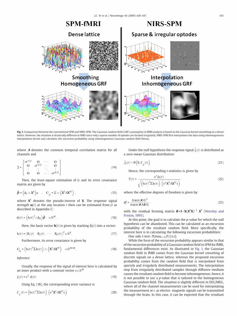
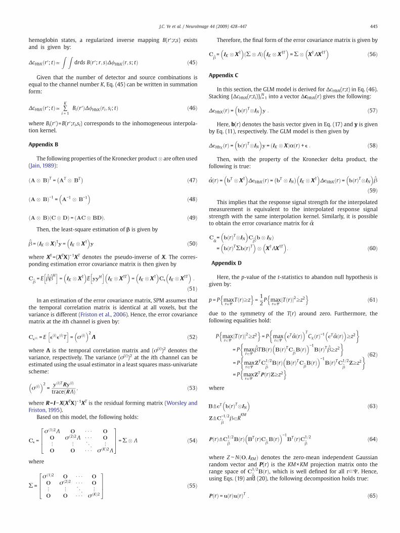
Fig.1. Comparison between the conventional SPM and NIRS-SPM. The Gaussian random field (GRF) assumption in fMRI analysis is based on the Gaussian kernel smoothing on a denselattice. However, the situation is drastically different in NIRS since only a sparse number of optodes are located irregularly. NIRS-SPM first interpolates the data using inhomogeneousinterpolation kernel and calculates the excursion probability using inhomogeneous Gaussian random field theory.

431J.C. Ye et al. / NeuroImage 44 (2009) 428–447

where Λ denotes the common temporal correlation matrix for allchannels and

Σ =

σ 1ð Þ2 O : : : OO σ 2ð Þ2 : : : Ov v O vO O : : : σ Kð Þ2

2664

3775 ð14Þ

Then, the least-square estimation of β and its error covariancematrix are given by

β̂ = IK � X†� �

y ; C ^

β=Σ� X†ΛX†T

� �; ð15Þ

where X† denotes the pseudo-inverse of X. The response signalstrength α(r) at the any location r then can be estimated from β asdescribed in Appendix C:

^α rð Þ = b rð ÞT�IM

� �β̂ aℝM : ð16Þ

Here, the basis vector b(r) is given by stacking Bi(r) into a vector:

b rð Þ = B1 rð Þ B2 rð Þ : : : BK rð Þ½ �TaℝK : ð17Þ

Furthermore, its error covariance is given by

C^α= b rð ÞT∑b rð Þ� �

� X†ΛX†T� �

aℝM×M: ð18Þ

Inference

Usually, the response of the signal of interest here is calculated byan inner product with a contrast vector caℝM

^χ rð Þ = cT ^α rð Þ ð19Þ

Using Eq. (18), the corresponding error variance is

C ^

χrð Þ = b rð ÞT∑b rð Þ

� �cTX†ΛX†Tc

� �ð20Þ

Under the null hypothesis the response signal χ̂ rð Þ is distributed asa zero-mean Gaussian distribution:

χ̂ rð ÞfN 0;C ^χrð Þ

� �ð21Þ

Hence, the corresponding t-statistics is given by

T rð Þ = cT^α rð Þffiffiffiffiffiffiffiffiffiffiffiffiffiffiffiffiffiffiffiffiffiffiffiffiffiffiffiffiffiffiffiffiffiffiffiffiffiffiffiffiffiffiffiffiffiffiffiffiffiffiffiffiffiffiffiffiffiffiffiffi

b rð ÞT∑b rð Þ� �

cTX†ΛX†Tc� �r ð22Þ

where the effective degrees of freedom is given by:

df =trace RΛð Þ2trace RΛRΛð Þ : ð23Þ

with the residual forming matrix R= I−X(XTX)−1 XT (Worsley andFriston, 1995).

At this point, the goal is to calculate the p-value for which the nullhypothesis can be abandoned. This can be calculated as an excursionprobability of the resultant random field. More specifically, theinterest here is in calculating the following excursion probabilities:

One side t-test: P{maxr∈ΨT(r)≥z}.While the form of the excursion probability appears similar to that

of the excursionprobability of aGaussian randomfield in SPM for fMRI,fundamental differences exist. As illustrated in Fig. 1, the Gaussianrandom field in fMRI comes from the Gaussian kernel smoothing ofdiscrete signals on a dense lattice, whereas the proposed excursionprobability comes from the random field that is interpolated fromsparsely and irregularly distributed measurements. The interpolationstep from irregularly distributed samples through diffusive mediumcauses the resultant random field to become inhomogeneous; hence, itis not possible to use a p-value that is tailored to the homogeneousGaussian random field. The situation is slightly different in EEG/MEG,where all of the channel measurements can be used for interpolatingthe measurement at r, as electro- magnetic signals can be transmittedthrough the brain. In this case, it can be expected that the resultant

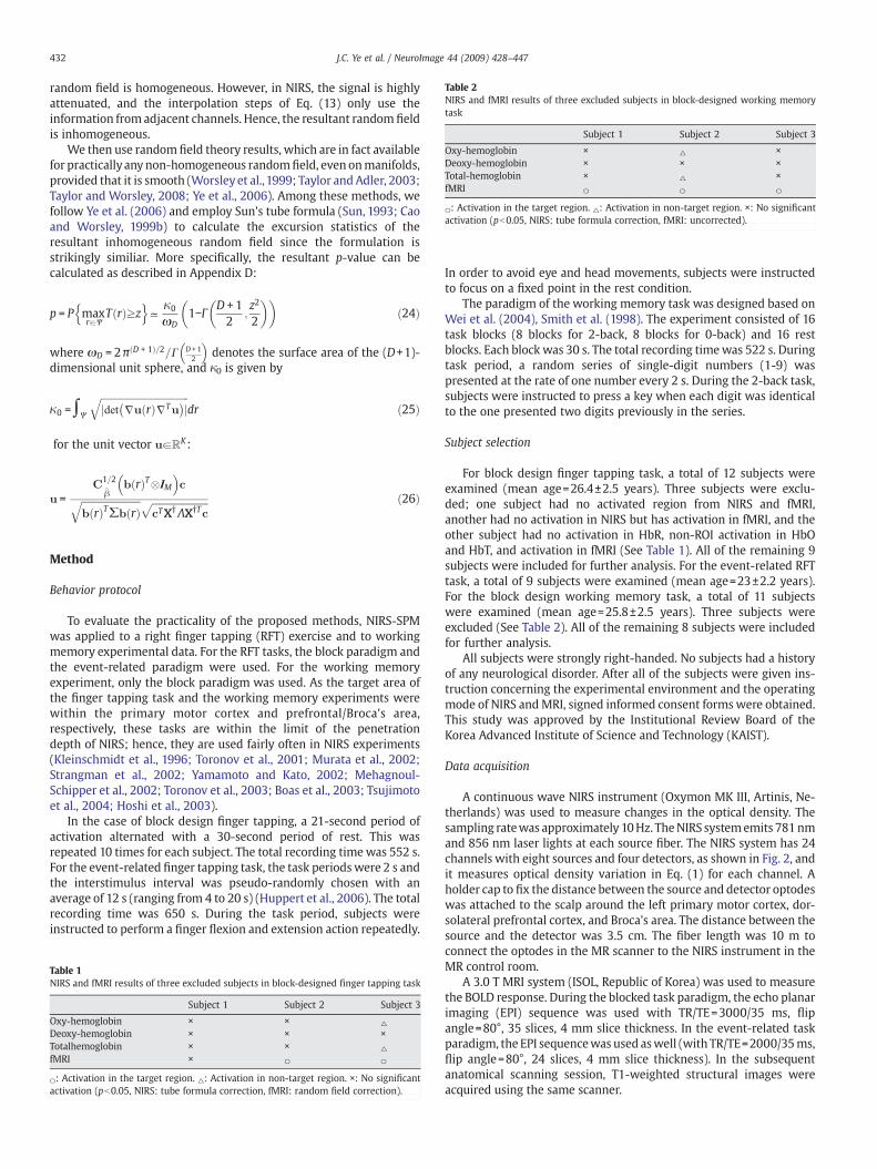
Table 2NIRS and fMRI results of three excluded subjects in block-designed working memorytask

Subject 1 Subject 2 Subject 3

Oxy-hemoglobin × △ ×Deoxy-hemoglobin × × ×Total-hemoglobin × △ ×fMRI ○ ○ ○

○: Activation in the target region. △: Activation in non-target region. ×: No significantactivation (pb0.05, NIRS: tube formula correction, fMRI: uncorrected).

432 J.C. Ye et al. / NeuroImage 44 (2009) 428–447

random field is homogeneous. However, in NIRS, the signal is highlyattenuated, and the interpolation steps of Eq. (13) only use theinformation from adjacent channels. Hence, the resultant random fieldis inhomogeneous.

We then use random field theory results, which are in fact availablefor practically any non-homogeneous randomfield, even onmanifolds,provided that it is smooth (Worsley et al.,1999; Taylor and Adler, 2003;Taylor and Worsley, 2008; Ye et al., 2006). Among these methods, wefollow Ye et al. (2006) and employ Sun's tube formula (Sun, 1993; Caoand Worsley, 1999b) to calculate the excursion statistics of theresultant inhomogeneous random field since the formulation isstrikingly similiar. More specifically, the resultant p-value can becalculated as described in Appendix D:

p = P maxraW

T rð Þzzn o

gκ0

ωD1−Γ

D + 12

;z2

2

ð24Þ

where ωD = 2π D + 1ð Þ=2=C D + 12

� �denotes the surface area of the (D+1)-

dimensional unit sphere, and κ0 is given by

κ0 = ∫Wffiffiffiffiffiffiffiffiffiffiffiffiffiffiffiffiffiffiffiffiffiffiffiffiffiffiffiffiffiffiffiffiffiffiffiffijdet ju rð ÞjTu

� �jq

dr ð25Þ

for the unit vector uaℝK :

u =C

1=2^

βb rð ÞT�IM

� �c

ffiffiffiffiffiffiffiffiffiffiffiffiffiffiffiffiffiffiffiffiffiffiffiffib rð ÞT∑b rð Þ

q ffiffiffiffiffiffiffiffiffiffiffiffiffiffiffiffiffiffiffiffiffiffifficTX†ΛX†Tc

p ð26Þ

Method

Behavior protocol

To evaluate the practicality of the proposed methods, NIRS-SPMwas applied to a right finger tapping (RFT) exercise and to workingmemory experimental data. For the RFT tasks, the block paradigm andthe event-related paradigm were used. For the working memoryexperiment, only the block paradigm was used. As the target area ofthe finger tapping task and the working memory experiments werewithin the primary motor cortex and prefrontal/Broca's area,respectively, these tasks are within the limit of the penetrationdepth of NIRS; hence, they are used fairly often in NIRS experiments(Kleinschmidt et al., 1996; Toronov et al., 2001; Murata et al., 2002;Strangman et al., 2002; Yamamoto and Kato, 2002; Mehagnoul-Schipper et al., 2002; Toronov et al., 2003; Boas et al., 2003; Tsujimotoet al., 2004; Hoshi et al., 2003).

In the case of block design finger tapping, a 21-second period ofactivation alternated with a 30-second period of rest. This wasrepeated 10 times for each subject. The total recording timewas 552 s.For the event-related finger tapping task, the task periodswere 2 s andthe interstimulus interval was pseudo-randomly chosen with anaverage of 12 s (ranging from 4 to 20 s) (Huppert et al., 2006). The totalrecording time was 650 s. During the task period, subjects wereinstructed to perform a finger flexion and extension action repeatedly.

Table 1NIRS and fMRI results of three excluded subjects in block-designed finger tapping task

Subject 1 Subject 2 Subject 3

Oxy-hemoglobin × × △

Deoxy-hemoglobin × × ×Totalhemoglobin × × △

fMRI × ○ ○

○: Activation in the target region. △: Activation in non-target region. ×: No significantactivation (pb0.05, NIRS: tube formula correction, fMRI: random field correction).

In order to avoid eye and head movements, subjects were instructedto focus on a fixed point in the rest condition.

The paradigm of the working memory task was designed based onWei et al. (2004), Smith et al. (1998). The experiment consisted of 16task blocks (8 blocks for 2-back, 8 blocks for 0-back) and 16 restblocks. Each block was 30 s. The total recording timewas 522 s. Duringtask period, a random series of single-digit numbers (1-9) waspresented at the rate of one number every 2 s. During the 2-back task,subjects were instructed to press a key when each digit was identicalto the one presented two digits previously in the series.

Subject selection

For block design finger tapping task, a total of 12 subjects wereexamined (mean age=26.4±2.5 years). Three subjects were exclu-ded; one subject had no activated region from NIRS and fMRI,another had no activation in NIRS but has activation in fMRI, and theother subject had no activation in HbR, non-ROI activation in HbOand HbT, and activation in fMRI (See Table 1). All of the remaining 9subjects were included for further analysis. For the event-related RFTtask, a total of 9 subjects were examined (mean age=23±2.2 years).For the block design working memory task, a total of 11 subjectswere examined (mean age=25.8±2.5 years). Three subjects wereexcluded (See Table 2). All of the remaining 8 subjects were includedfor further analysis.

All subjects were strongly right-handed. No subjects had a historyof any neurological disorder. After all of the subjects were given ins-truction concerning the experimental environment and the operatingmode of NIRS andMRI, signed informed consent formswere obtained.This study was approved by the Institutional Review Board of theKorea Advanced Institute of Science and Technology (KAIST).

Data acquisition

A continuous wave NIRS instrument (Oxymon MK III, Artinis, Ne-therlands) was used to measure changes in the optical density. Thesampling ratewas approximately 10Hz. TheNIRS systememits 781nmand 856 nm laser lights at each source fiber. The NIRS system has 24channels with eight sources and four detectors, as shown in Fig. 2, andit measures optical density variation in Eq. (1) for each channel. Aholder cap to fix the distance between the source and detector optodeswas attached to the scalp around the left primary motor cortex, dor-solateral prefrontal cortex, and Broca's area. The distance between thesource and the detector was 3.5 cm. The fiber length was 10 m toconnect the optodes in the MR scanner to the NIRS instrument in theMR control room.

A 3.0 T MRI system (ISOL, Republic of Korea) was used to measurethe BOLD response. During the blocked task paradigm, the echo planarimaging (EPI) sequence was used with TR/TE=3000/35 ms, flipangle=80°, 35 slices, 4 mm slice thickness. In the event-related taskparadigm, the EPI sequencewas used aswell (with TR/TE=2000/35ms,flip angle=80°, 24 slices, 4 mm slice thickness). In the subsequentanatomical scanning session, T1-weighted structural images wereacquired using the same scanner.

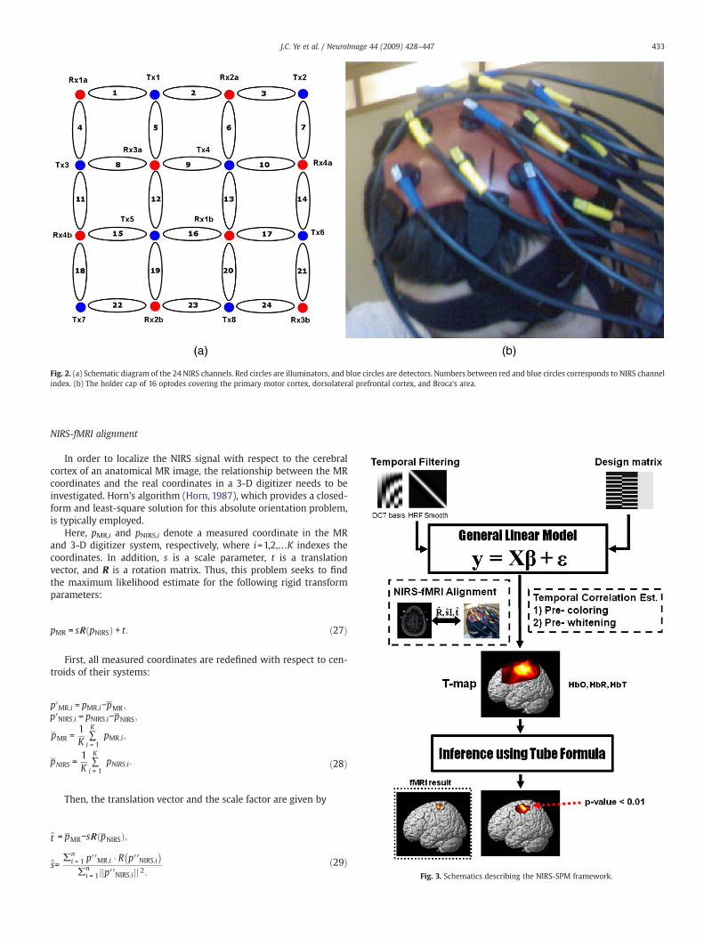
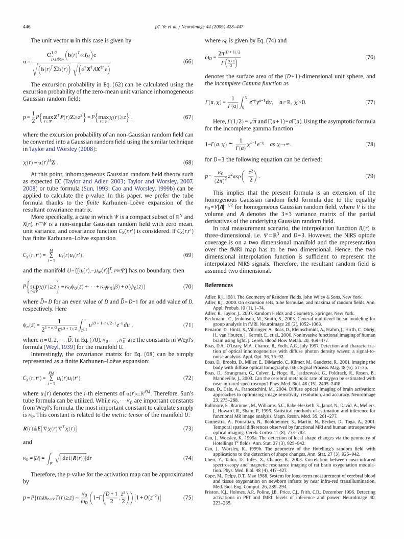
Fig. 2. (a) Schematic diagram of the 24 NIRS channels. Red circles are illuminators, and blue circles are detectors. Numbers between red and blue circles corresponds to NIRS channelindex. (b) The holder cap of 16 optodes covering the primary motor cortex, dorsolateral prefrontal cortex, and Broca's area.

Fig. 3. Schematics describing the NIRS-SPM framework.

433J.C. Ye et al. / NeuroImage 44 (2009) 428–447

NIRS-fMRI alignment

In order to localize the NIRS signal with respect to the cerebralcortex of an anatomical MR image, the relationship between the MRcoordinates and the real coordinates in a 3-D digitizer needs to beinvestigated. Horn's algorithm (Horn, 1987), which provides a closed-form and least-square solution for this absolute orientation problem,is typically employed.

Here, pMR,i and pNIRS,i denote a measured coordinate in the MRand 3-D digitizer system, respectively, where i=1,2,…K indexes thecoordinates. In addition, s is a scale parameter, t is a translationvector, and R is a rotation matrix. Thus, this problem seeks to findthe maximum likelihood estimate for the following rigid transformparameters:

pMR = sR pNIRSð Þ + t: ð27Þ

First, all measured coordinates are redefined with respect to cen-troids of their systems:

p′MR;i = pMR;i−pMR;p′NIRS;i = pNIRS;i−pNIRS;

pMR =1K

∑K

i = 1pMR;i;

pNIRS =1K

∑K

i = 1pNIRS;i: ð28Þ

Then, the translation vector and the scale factor are given by

^t = pMR−sR pNIRSð Þ;

s^=∑n

i = 1 p′′MR;i � R p′′NIRS;i� �

∑ni = 1jjp′′NIRS;ijj 2:

ð29Þ

434 J.C. Ye et al. / NeuroImage 44 (2009) 428–447

Let pi′=(xi′, yi′, zi′)T and

AMR;i =

0 −χi′ −yi′ −zi′χi′ 0 −zi′ yi′yi′ zi′ 0 −χi′zi′ −yi′ χi′ 0

2664

3775; BNIRS;i =

0 −χi′ −yi′ −zi′χi′ 0 zi′ −yi′yi′ −zi′ 0 χi′zi′ yi′ −χi′ 0

2664

3775: ð30Þ

If we define the matrix N as

N = ∑K

i = 1BT

NIRS;iAMR;i: ð31Þ

The vector q, which is directly related to the rotation parameters, isthe eigenvector corresponding to the maximum eigenvalue of the

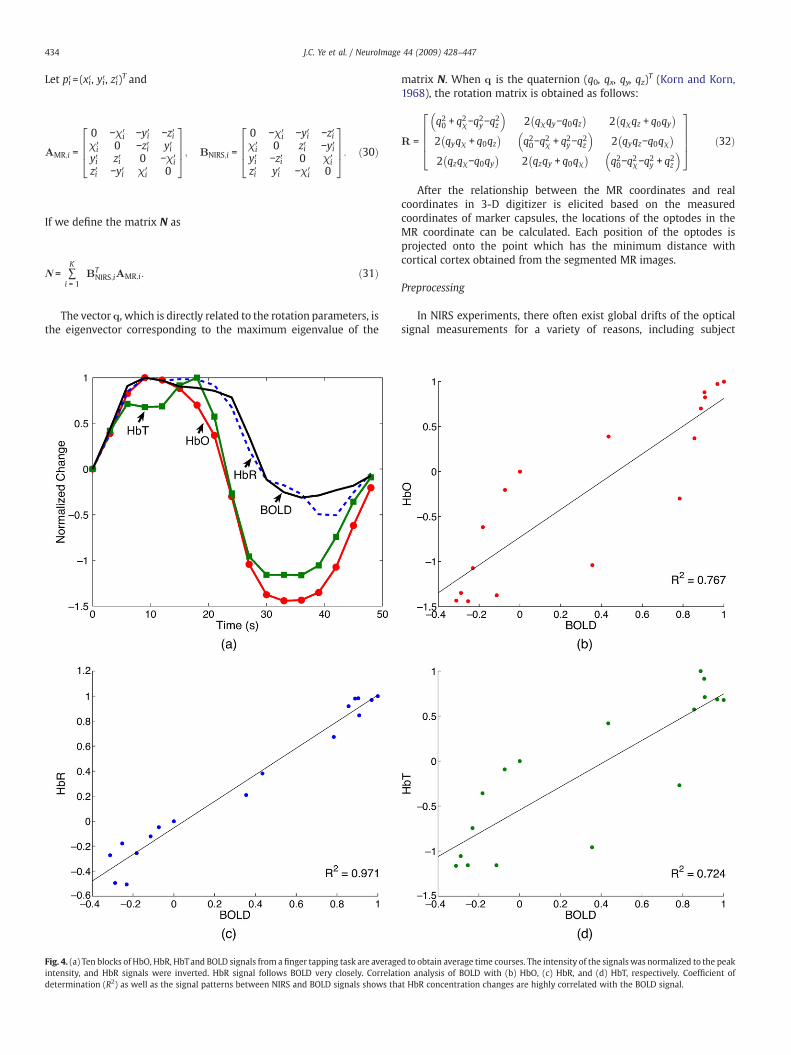
Fig. 4. (a) Ten blocks of HbO, HbR, HbTand BOLD signals from a finger tapping task are averageintensity, and HbR signals were inverted. HbR signal follows BOLD very closely. Correlatdetermination (R2) as well as the signal patterns between NIRS and BOLD signals shows tha

matrix N. When q is the quaternion (q0, qx, qy, qz)T (Korn and Korn,1968), the rotation matrix is obtained as follows:

R =

q20 + q2χ−q2y−q2z

� �2 qχqy−q0qz� �

2 qχqz + q0qy� �

2 qyqχ + q0qz� �

q20−q2χ + q2y−q2z

� �2 qyqz−q0qχ� �

2 qzqχ−q0qy� �

2 qzqy + q0qχ� �

q20−q2χ−q2y + q2z

� �

26664

37775 ð32Þ

After the relationship between the MR coordinates and realcoordinates in 3-D digitizer is elicited based on the measuredcoordinates of marker capsules, the locations of the optodes in theMR coordinate can be calculated. Each position of the optodes isprojected onto the point which has the minimum distance withcortical cortex obtained from the segmented MR images.

Preprocessing

In NIRS experiments, there often exist global drifts of the opticalsignal measurements for a variety of reasons, including subject

d to obtain average time courses. The intensity of the signals was normalized to the peakion analysis of BOLD with (b) HbO, (c) HbR, and (d) HbT, respectively. Coefficient oft HbR concentration changes are highly correlated with the BOLD signal.

435J.C. Ye et al. / NeuroImage 44 (2009) 428–447

movement during the experiment, vasomotion, blood pressurevariation, long-term physiological changes or instrumental instability.Moreover, the amplitude of the global drift is often comparable to thatof the signal from a brain activation process. In order to eliminate theglobal trend and to improve the signal-to-noise ratio, a highpass filterbased on a discrete cosine transform (DCT) was employed, as iscurrently implemented in SPM (Friston et al., 2006). For the NIRS dataof the finger tapping task, a cutoff frequency of 1/60 Hz was used. Forthe NIRS data of the working memory task, a cutoff frequency of1/128 Hz was used, as the task related frequency was 1/120 Hz.

After detrending, “short-range” temporal correlation continues toexist in NIRS data. This means that the residual signal at the specifictime is correlated with its temporal neighbors. In order to obtain thecorrect t-statistics in Eq. (22), the temporal correlation structure ofNIRS should be investigated. The “precoloring” method (Worsley andFriston, 1995) was compared with the “prewhitening” method(Bullmore et al., 1996; Friston et al., 2002), both initially proposed forthe fMRI model (Friston et al., 2006). Currently, most of the NIRS-GLManalysis have employed the prewhiteningmethod (Plichta et al., 2006,2007; Koh et al., 2007; Hofmann et al., 2008). In cases where thetemporal smoothing is strong enough to swamp any intrinsic temporal

Fig. 5. (a) Paired t-test results to compare two paired group among the following four data seHbR within ROI (wROI) and prewhitened HbR outside ROI (wOUT). (b) Paired t-test results tois downsampled after anti-aliasing filteringwithin ROI (wdaROI), outside ROI (wdaOUT), prewoutside ROI (wdOUT). Downsampling factor was 10. (c) Paired t-test results to compare two pprecolored HbO outside ROI (cOUT–HbO), prewhitened HbO which is downsampled after asignificant difference was observed in cROI and cOUT (pb0.035), such significant differencsignificant difference betweenwdROI and wdOUT (pb0.389) was not observed because of thsignificant difference between wdaROI and wdaOUT (pb0.042) was detected. Note that in cathe t-map within and outside ROI, whereas the precolored HbO still provide statistically meato prewhitening method in estimating the temporal correlations. In these figures, the t-valu

correlation, the precoloringmethod is preferred. Specifically, if the full-width-at-half-maximum (FWHM) value of the smoothing kernel issufficiently large, temporal correlation induced by the smoothingprocess can be obtained without an intrinsic temporal correlation:

Λ = SVST≈SST : ð33Þ

Here, Λ is a temporal correlation matrix, V is an intrinsic temporalcorrelation and S is a smoothing matrix that is typically derived fromthe canonical HRF or Gaussian smoothing kernel (Friston et al., 2000).As the transfer function of HRF is in the frequencies of modeledneuronal signals, the canonical HRF was employed for the temporalsmoothing of the NIRS time-series. An alternative way method,prewhitening involveswhitening the data using the smoothingmatrixS that is derived from the intrinsic temporal correlation V:

S =K−1; ð34Þ

where KKT=V and V is estimated via restricted maximum likelihood(ReML) (Friston et al., 2002). If the estimated intrinsic temporal

ts: precolored HbR within ROI (cROI), precolored HbR outside ROI (cOUT), prewhitenedcompare two paired group among the following four data sets: prewhitened HbR whichhitened HbRwhich is downsampledwithout anti-aliasing filteringwithin ROI (wdROI),

aired group among the following four data sets: precolored HbOwithin ROI (cROI–HbO),nti-aliasing filtering within ROI (wdaROI–HbO), outside ROI (wdaROI–HbO). Althoughe was not observed in wROI and wOUT (pb0.086). In case of downsampled HbR, anye aliasing effect. However, when the antialiasing filter was used before downsampling, ase of the prewhitened HbO, no significant difference (pb0.070) was observed betweenning full differences (pb0.038). This result supports that precoloring method is superiores indicate the averaged t-value within and outside ROI.

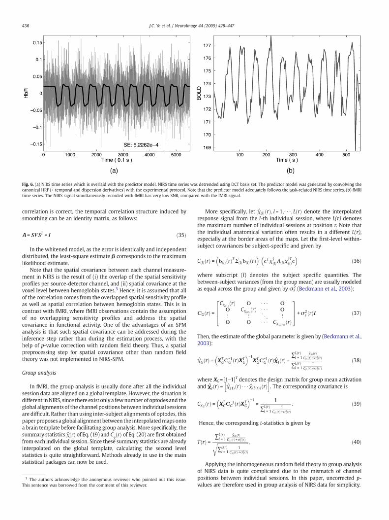
Fig. 6. (a) NIRS time series which is overlaid with the predictor model. NIRS time series was detrended using DCT basis set. The predictor model was generated by convolving thecanonical HRF (+ temporal and dispersion derivatives) with the experimental protocol. Note that the predictor model adequately follows the task-related NIRS time series. (b) fMRItime series. The NIRS signal simultaneously recorded with fMRI has very low SNR, compared with the fMRI signal.

436 J.C. Ye et al. / NeuroImage 44 (2009) 428–447

correlation is correct, the temporal correlation structure induced bysmoothing can be an identity matrix, as follows:

Λ = SVST = I ð35Þ

In the whitened model, as the error is identically and independentdistributed, the least-square estimate β corresponds to the maximumlikelihood estimate.

Note that the spatial covariance between each channel measure-ment in NIRS is the result of (i) the overlap of the spatial sensitivityprofiles per source-detector channel, and (ii) spatial covariance at thevoxel level between hemoglobin states.3 Hence, it is assumed that allof the correlation comes from the overlapped spatial sensitivity profileas well as spatial correlation between hemoglobin states. This is incontrast with fMRI, where fMRI observations contain the assumptionof no overlapping sensitivity profiles and address the spatialcovariance in functional activity. One of the advantages of an SPManalysis is that such spatial covariance can be addressed during theinference step rather than during the estimation process, with thehelp of p-value correction with random field theory. Thus, a spatialpreprocessing step for spatial covariance other than random fieldtheory was not implemented in NIRS-SPM.

Group analysis

In fMRI, the group analysis is usually done after all the individualsession data are aligned on a global template. However, the situation isdifferent inNIRS, since there exist only a fewnumberof optodes and theglobal alignments of the channel positions between individual sessionsare difficult. Rather than using inter-subject alignments of optodes, thispaper proposes a global alignment between the interpolatedmaps ontoa brain template before facilitating group analysis. More specifically, thesummary statistics χ̂ rð Þ of Eq. (19) and C

χ̂rð Þ of Eq. (20) are first obtained

from each individual session. Since these summary statistics are alreadyinterpolated on the global template, calculating the second levelstatistics is quite straightforward. Methods already in use in the mainstatistical packages can now be used.

3 The authors acknowledge the anonymous reviewer who pointed out this issue.This sentence was borrowed from the comment of this reviewer.

More specifically, let χ̂ lð Þ rð Þ; l = 1;: : :; L rð Þ denote the interpolatedresponse signal from the l-th individual session, where L(r) denotesthe maximum number of individual sessions at position r. Note thatthe individual anatomical variation often results in a different L(r),especially at the border areas of the maps. Let the first-level within-subject covariances be subject-specific and given by

C lð Þ rð Þ = b lð Þ rð ÞTΣ lð Þb lð Þ rð Þ� �

cTχ†lð ÞΛ lð Þχ

†Tlð Þc

� �ð36Þ

where subscript (l) denotes the subject specific quantities. Thebetween-subject variances (from the group mean) are usually modeledas equal across the group and given by σs

2 (Beckmann et al., 2003):

CG rð Þ =Cχ 1ð Þ rð Þ O : : : O

O Cχ 2ð Þ rð Þ : : : Ov v O vO O : : : Cχ L rð Þð Þ rð Þ

2664

3775 + σ2

s rð ÞI ð37Þ

Then, the estimate of the global parameter is given by (Beckmann et al.,2003):

χ̂G rð Þ = XTGC

−1G rð ÞXT

G

� �−1XT

GC−1G rð Þχ̂I rð Þ =

∑L rð Þl = 1

χ̂ lð Þ rð ÞC lð Þ rð Þ +σ2

s rð Þ

∑L rð Þl = 1

1^

C lð Þ rð Þ +σ2s rð Þ

ð38Þ

where XG=[1⋯1]T denotes the design matrix for group mean activationand χ̂I rð Þ = χ̂ 1ð Þ rð Þ: : : χ̂ L rð Þð Þ rð Þ

h i. The corresponding covariance is

CχGrð Þ = XT

GC−1G rð ÞXT

G

� �−1=

1

∑L rð Þl = 1

1^

C lð Þ rð Þ +σ2s rð Þ

: ð39Þ

Hence, the corresponding t-statistics is given by

T rð Þ =∑L rð Þ

l = 1χ̂ lð Þ rð Þ

C lð Þ rð Þ +σ2s rð Þffiffiffiffiffiffiffiffiffiffiffiffiffiffiffiffiffiffiffiffiffiffiffiffiffiffiffiffiffi

∑L rð Þl = 1

1^

C lð Þ rð Þ +σ2s rð Þ

r ; ð40Þ

Applying the inhomogeneous random field theory to group analysisof NIRS data is quite complicated due to the mismatch of channelpositions between individual sessions. In this paper, uncorrected p-values are therefore used in group analysis of NIRS data for simplicity.

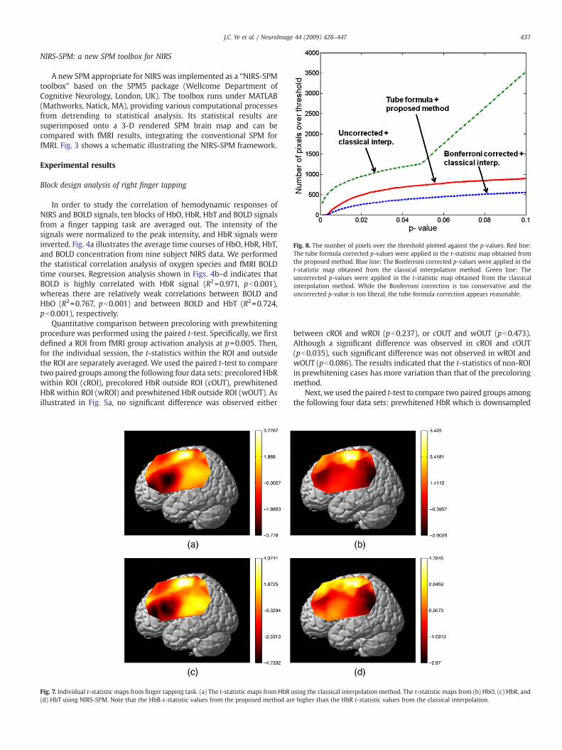
Fig. 8. The number of pixels over the threshold plotted against the p-values. Red line:The tube formula corrected p-values were applied in the t-statistic map obtained fromthe proposed method. Blue line: The Bonferroni corrected p-values were applied in thet-statistic map obtained from the classical interpolation method. Green line: Theuncorrected p-values were applied in the t-statistic map obtained from the classicalinterpolation method. While the Bonferroni correction is too conservative and theuncorrected p-value is too liberal, the tube formula correction appears reasonable.

437J.C. Ye et al. / NeuroImage 44 (2009) 428–447

NIRS-SPM: a new SPM toolbox for NIRS

A new SPM appropriate for NIRS was implemented as a “NIRS-SPMtoolbox” based on the SPM5 package (Wellcome Department ofCognitive Neurology, London, UK). The toolbox runs under MATLAB(Mathworks, Natick, MA), providing various computational processesfrom detrending to statistical analysis. Its statistical results aresuperimposed onto a 3-D rendered SPM brain map and can becompared with fMRI results, integrating the conventional SPM forfMRI. Fig. 3 shows a schematic illustrating the NIRS-SPM framework.

Experimental results

Block design analysis of right finger tapping

In order to study the correlation of hemodynamic responses ofNIRS and BOLD signals, ten blocks of HbO, HbR, HbT and BOLD signalsfrom a finger tapping task are averaged out. The intensity of thesignals were normalized to the peak intensity, and HbR signals wereinverted. Fig. 4a illustrates the average time courses of HbO, HbR, HbT,and BOLD concentration from nine subject NIRS data. We performedthe statistical correlation analysis of oxygen species and fMRI BOLDtime courses. Regression analysis shown in Figs. 4b–d indicates thatBOLD is highly correlated with HbR signal (R2=0.971, pb0.001),whereas there are relatively weak correlations between BOLD andHbO (R2=0.767, pb0.001) and between BOLD and HbT (R2=0.724,pb0.001), respectively.

Quantitative comparison between precoloring with prewhiteningprocedure was performed using the paired t-test. Specifically, we firstdefined a ROI from fMRI group activation analysis at p=0.005. Then,for the individual session, the t-statistics within the ROI and outsidethe ROI are separately averaged. We used the paired t-test to comparetwo paired groups among the following four data sets: precolored HbRwithin ROI (cROI), precolored HbR outside ROI (cOUT), prewhitenedHbR within ROI (wROI) and prewhitened HbR outside ROI (wOUT). Asillustrated in Fig. 5a, no significant difference was observed either

Fig. 7. Individual t-statistic maps from finger tapping task. (a) The t-statistic maps from HbR u(d) HbT using NIRS-SPM. Note that the HbR-t-statistic values from the proposed method ar

between cROI and wROI (pb0.237), or cOUT and wOUT (pb0.473).Although a significant difference was observed in cROI and cOUT(pb0.035), such significant difference was not observed in wROI andwOUT (pb0.086). The results indicated that the t-statistics of non-ROIin prewhitening cases has more variation than that of the precoloringmethod.

Next, we used the paired t-test to compare two paired groups amongthe following four data sets: prewhitened HbR which is downsampled

sing the classical interpolation method. The t-statistic maps from (b) HbO, (c) HbR, ande higher than the HbR t-statistic values from the classical interpolation.

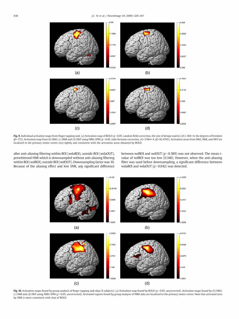
Fig. 9. Individual activationmaps from finger tapping task. (a) Activationmap of BOLD (pb0.05, random field correction, the size of designmatrix (sX)=184×4, the degrees of freedomdf=172). Activation map from (b) HbO, (c) HbR and (d) HbT using NIRS-SPM (pb0.05, tube formula correction, sX=5384×4, df=82.4705). Activation areas fromHbO, HbR, and HbT arelocalized to the primary motor cortex very tightly and consistent with the activation areas obtained by BOLD.

438 J.C. Ye et al. / NeuroImage 44 (2009) 428–447

after anti-aliasing filtering within ROI (wdaROI), outside ROI (wdaOUT),prewhitened HbRwhich is downsampled without anti-aliasing filteringwithin ROI (wdROI), outside ROI (wdOUT). Downsampling factorwas 10.Because of the aliasing effect and low SNR, any significant difference

Fig. 10. Activation maps found by group analysis of finger tapping task data (9 subjects). (a) A(c) HbR and (d) HbT using NIRS-SPM (pb0.05, uncorrected). Activated regions found by groupby HbR is more consistent with that of BOLD.

between wdROI and wdOUT (pb0.389) was not observed. The mean t-value of wdROI was too low (0.346). However, when the anti-aliasingfilter was used before downsampling, a significant difference betweenwdaROI and wdaOUT (pb0.042) was detected.

ctivation map found by BOLD (pb0.05, uncorrected). Activation maps found by (b) HbO,analysis of NIRS data are localized to the primary motor cortex. Note that activated area

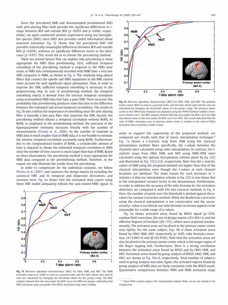
Fig. 12. Receiver operation characteristics (ROC) for HbO, HbR, and HbT. The primarymotor cortex (BA4) is used as a ground-truth, and the false alarm ratio and hit ratio arecalculated by changing the threshold values for the group t-map. The primary motorcortex in the SPM-brain template was depicted using the WFR PickAtlas toolbox (www.ansir.wfubmc.edu). The ROC analysis showed that the area under the ROC curve for HbRwas almost same as the area under the ROC curve for HbO. This result indicated that theratio of HbR's activation area in primary motor cortex is similar to the ratio of HbOsactivation area in primary motor cortex.

439J.C. Ye et al. / NeuroImage 44 (2009) 428–447

Since the precolored HbR and downsampled prewhitened HbOwith anti-aliasing filter both provide the significant differences in t-maps between ROI and outside ROI (pb0.035 and pb0.042, respec-tively), we again conducted another experiment using oxy-hemoglo-bin species (HbO) since HbO also provides useful information aboutneuronal activation. Fig. 5c shows that the precolored HbO stillprovides statistically meaningful differences between ROI and outsideROI (pb0.038), whereas no significant difference exists in the lattercases (pb0.07). This result led us to choose the precoloring method.

There are several factors that can explain why precoloring is moreappropriate for NIRS than prewhitening. First, sufficient temporalsmoothing of the precoloring method is required in the NIRS timeseries as NIRS data simultaneously recorded with fMRI have a very lowSNR compared to fMRI, as shown in Fig. 6. The relatively long opticalfibers that connect the optode and NIRS equipment in the MRI controlroom account for such significant signal attenuation. Thus, in order toimprove the SNR, sufficient temporal smoothing is necessary in thepreprocessing step. In case of prewhitening method, the temporalsmoothing matrix is derived from the intrinsic temporal correlationusing unsmoothed NIRS data that have a poor SNR. These increases theprobability that prewhitening produces some bias due to the differencebetween the estimated and actual temporal correlations. The results inFig. 5b also confirm the importance of smoothing since the anti-aliasingfilter is basically a low pass filter that improves the SNR. Second, theprecoloring method obtains a temporal correlation without ReML. InReML as employed in the prewhitening method, the precision of thehyperparameter estimates increases linearly with the number ofmeasurements (Friston et al., 2006). As the number of channels inNIRS data ismuch smaller than in fMRI data, it is not feasible to estimatethe intrinsic temporal correlation accurately using ReML. Furthermore,due to the computational burden of ReML, a considerable amount oftime is required to obtain the estimated temporal correlation in NIRSsince the number of time courses ismuch larger than that of fMRI. Basedon these observations, the precoloring method is more appropriate forNIRS data compared to the prewhitening method. Therefore, in thesequel, we only illustrate the results from the precoloring.

In order to compensate for the individual variation, we followPlichta et al. (2007) and construct the design matrix by including thecanonical HRF, and its temporal and dispersion derivatives, andconstant term. Fig. 6a shows that the estimated time course usingthese HRF model adequately follows the task-related NIRS signal. In

Fig. 11. Receiver operation characteristics (ROC) for HbO, HbR, and HbT. The fMRIactivation map at p=0.005 is used as a ground-truth, and the false alarm ratio and hitratio are calculated by changing the threshold values for the group t-map. The ROCanalysis showed that the area under the ROC curve for HbR was largest, indicating thatHbR activation map can predict the BOLD activation map more reliably.

order to support the superiority of the proposed method, wecompared our results with that of classic interpolation technique.4

Fig. 7a shows a t-statistic map from HbR using the classicalinterpolation method. More specifically, the t-values between thechannels were calculated using cubic interpolation. In contrast, the t-statistic maps from HbO, HbR, and HbT using NIRS-SPM werecalculated using the optimal interpolation scheme given by Eq. (22)and illustrated in Fig. 7(b)(c)(d), respectively. Note that the t-statisticvalues of HbR using the proposed method are higher than that of theclassical interpolation even though the t-values at each channellocations are identical. The main reason for such increases in t-statistics is that our interpolation scheme in Eq. (22) is non-linear dueto the interpolated variance terms in the denominator. Furthermore,in order to address the accuracy of the tube formula for the activationdetection, we compared it with the two classical methods in Fig. 8.Here, the number of pixels over the threshold is plotted against the p-values for various correction method. While the Bonferroni correctionusing the classical interpolation is too conservative and the uncor-rected p- value is too liberal, our tube formula correction appears to bereasonable for a wide range of p-values.

Fig. 9a shows activated areas found by BOLD signal (pb0.05,random field correction, the size of design matrix (sX)=184×4, and theeffective degrees of freedom (df)=172), which were acquired simulta-neously. The activated areas are localized to the primary motor cortexvery tightly. For the same subject, Figs. 9b–d show activation areasfound by HbO, HbR, HbT, respectively (pb0.05, tube formula correc-tion, sX=5384×4, and df=82.4705). Note that the activation areas arealso localized to the primarymotor cortex which is the target region ofthe finger tapping task. Furthermore, there is a strong correlationbetween the activation areas found by BOLD and by HbO, HbR, andHbT. Activation areas found by group analysis of BOLD, HbO, HbR, andHbT, are shown in Fig. 10a–d, respectively. Total number of subjectsused in group analysis was nine. Again, the activated regions found bygroup analysis of NIRS data are fairly consistent with the BOLD result.Quantitative comparisons between NIRS and fMRI activation maps

4 Since fOSA cannot analyze the interpolated random field, we do not include it forcomparison.

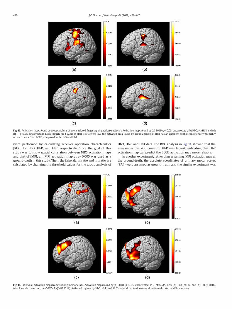
Fig. 13. Activation maps found by group analysis of event-related finger tapping task (9 subjects). Activation maps found by (a) BOLD (pb0.05, uncorrected), (b) HbO, (c) HbR and (d)HbT (pb0.05, uncorrected). Even though the t-value of HbR is relatively low, the activated area found by group analysis of HbR has an excellent spatial consistence with highlyactivated area from BOLD, compared with HbO and HbT.

440 J.C. Ye et al. / NeuroImage 44 (2009) 428–447

were performed by calculating receiver operation characteristics(ROC) for HbO, HbR, and HbT, respectively. Since the goal of thisstudy was to show spatial correlation between NIRS activation mapsand that of fMRI, an fMRI activation map at p=0.005 was used as aground-truth in this study. Then, the false alarm ratio and hit ratio arecalculated by changing the threshold values for the group analysis of

Fig. 14. Individual activation maps fromworking memory task. Activation maps found by (a)tube formula correction, sX=5067×7, df=83.8212). Activated regions by HbO, HbR, and HbT

HbO, HbR, and HbT data. The ROC analysis in Fig. 11 showed that thearea under the ROC curve for HbR was largest, indicating that HbRactivation map can predict the BOLD activation map more reliably.

In another experiment, rather than assuming fMRI activationmap asthe ground-truth, the absolute coordinates of primary motor cortex(BA4) were assumed as ground-truth, and the similar experiment was

BOLD (pb0.05, uncorrected, sX=174×7, df=159), (b) HbO, (c) HbR and (d) HbT (pb0.05,are localized to dorsolateral prefrontal cortex and Broca's area.

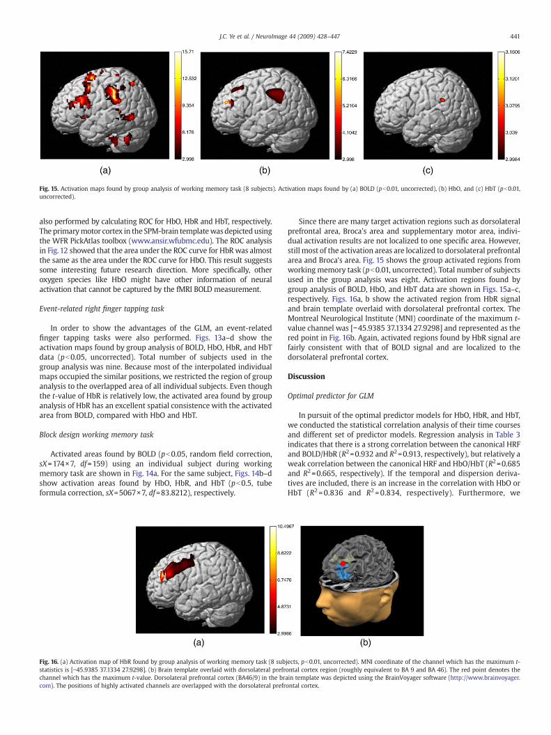
Fig. 15. Activation maps found by group analysis of working memory task (8 subjects). Activation maps found by (a) BOLD (pb0.01, uncorrected), (b) HbO, and (c) HbT (pb0.01,uncorrected).

441J.C. Ye et al. / NeuroImage 44 (2009) 428–447

also performed by calculating ROC for HbO, HbR and HbT, respectively.The primarymotor cortex in the SPM-brain templatewasdepictedusingthe WFR PickAtlas toolbox (www.ansir.wfubmc.edu). The ROC analysisin Fig. 12 showed that the area under the ROC curve for HbR was almostthe same as the area under the ROC curve for HbO. This result suggestssome interesting future research direction. More specifically, otheroxygen species like HbO might have other information of neuralactivation that cannot be captured by the fMRI BOLD measurement.

Event-related right finger tapping task

In order to show the advantages of the GLM, an event-relatedfinger tapping tasks were also performed. Figs. 13a–d show theactivation maps found by group analysis of BOLD, HbO, HbR, and HbTdata (pb0.05, uncorrected). Total number of subjects used in thegroup analysis was nine. Because most of the interpolated individualmaps occupied the similar positions, we restricted the region of groupanalysis to the overlapped area of all individual subjects. Even thoughthe t-value of HbR is relatively low, the activated area found by groupanalysis of HbR has an excellent spatial consistence with the activatedarea from BOLD, compared with HbO and HbT.

Block design working memory task

Activated areas found by BOLD (pb0.05, random field correction,sX=174×7, df=159) using an individual subject during workingmemory task are shown in Fig. 14a. For the same subject, Figs. 14b–dshow activation areas found by HbO, HbR, and HbT (pb0.5, tubeformula correction, sX=5067×7, df=83.8212), respectively.

Fig. 16. (a) Activation map of HbR found by group analysis of working memory task (8 substatistics is [−45.9385 37.1334 27.9298]. (b) Brain template overlaid with dorsolateral prefrchannel which has the maximum t-value. Dorsolateral prefrontal cortex (BA46/9) in the bracom). The positions of highly activated channels are overlapped with the dorsolateral prefr

Since there are many target activation regions such as dorsolateralprefrontal area, Broca's area and supplementary motor area, indivi-dual activation results are not localized to one specific area. However,still most of the activation areas are localized to dorsolateral prefrontalarea and Broca's area. Fig. 15 shows the group activated regions fromworking memory task (pb0.01, uncorrected). Total number of subjectsused in the group analysis was eight. Activation regions found bygroup analysis of BOLD, HbO, and HbT data are shown in Figs. 15a–c,respectively. Figs. 16a, b show the activated region from HbR signaland brain template overlaid with dorsolateral prefrontal cortex. TheMontreal Neurological Institute (MNI) coordinate of the maximum t-value channel was [−45.9385 37.1334 27.9298] and represented as thered point in Fig. 16b. Again, activated regions found by HbR signal arefairly consistent with that of BOLD signal and are localized to thedorsolateral prefrontal cortex.

Discussion

Optimal predictor for GLM

In pursuit of the optimal predictor models for HbO, HbR, and HbT,we conducted the statistical correlation analysis of their time coursesand different set of predictor models. Regression analysis in Table 3indicates that there is a strong correlation between the canonical HRFand BOLD/HbR (R2=0.932 and R2=0.913, respectively), but relatively aweak correlation between the canonical HRF and HbO/HbT (R2=0.685and R2=0.665, respectively). If the temporal and dispersion deriva-tives are included, there is an increase in the correlation with HbO orHbT (R2 =0.836 and R2 =0.834, respectively). Furthermore, we

jects, pb0.01, uncorrected). MNI coordinate of the channel which has the maximum t-ontal cortex region (roughly equivalent to BA 9 and BA 46). The red point denotes thein template was depicted using the BrainVoyager software (http://www.brainvoyager.ontal cortex.

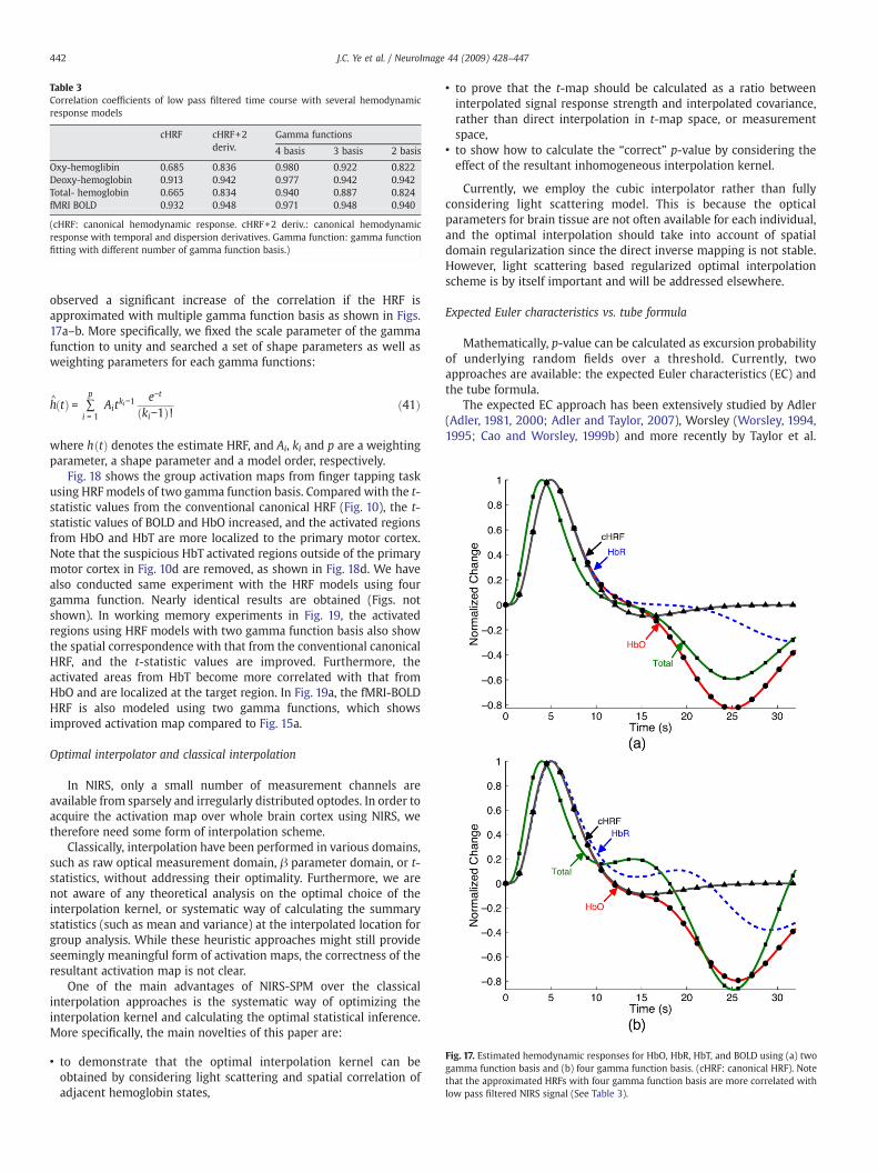
Fig. 17. Estimated hemodynamic responses for HbO, HbR, HbT, and BOLD using (a) twogamma function basis and (b) four gamma function basis. (cHRF: canonical HRF). Notethat the approximated HRFs with four gamma function basis are more correlated withlow pass filtered NIRS signal (See Table 3).

Table 3Correlation coefficients of low pass filtered time course with several hemodynamicresponse models

cHRF cHRF+2deriv.

Gamma functions

4 basis 3 basis 2 basis

Oxy-hemoglibin 0.685 0.836 0.980 0.922 0.822Deoxy-hemoglobin 0.913 0.942 0.977 0.942 0.942Total- hemoglobin 0.665 0.834 0.940 0.887 0.824fMRI BOLD 0.932 0.948 0.971 0.948 0.940

(cHRF: canonical hemodynamic response. cHRF+2 deriv.: canonical hemodynamicresponse with temporal and dispersion derivatives. Gamma function: gamma functionfitting with different number of gamma function basis.)

442 J.C. Ye et al. / NeuroImage 44 (2009) 428–447

observed a significant increase of the correlation if the HRF isapproximated with multiple gamma function basis as shown in Figs.17a–b. More specifically, we fixed the scale parameter of the gammafunction to unity and searched a set of shape parameters as well asweighting parameters for each gamma functions:

h^tð Þ = ∑

p

i = 1Aitki−1

e−t

ki−1ð Þ! ð41Þ

where h tð Þ denotes the estimate HRF, and Ai, ki and p are a weightingparameter, a shape parameter and a model order, respectively.

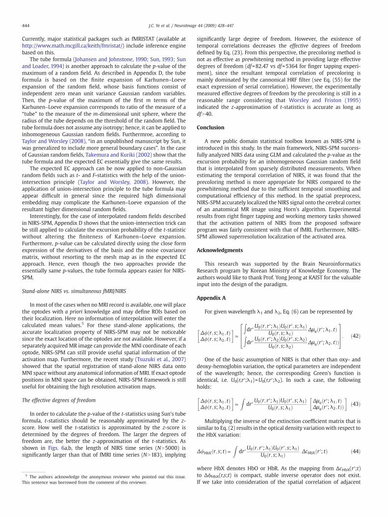
Fig. 18 shows the group activation maps from finger tapping taskusing HRF models of two gamma function basis. Compared with the t-statistic values from the conventional canonical HRF (Fig. 10), the t-statistic values of BOLD and HbO increased, and the activated regionsfrom HbO and HbT are more localized to the primary motor cortex.Note that the suspicious HbT activated regions outside of the primarymotor cortex in Fig. 10d are removed, as shown in Fig. 18d. We havealso conducted same experiment with the HRF models using fourgamma function. Nearly identical results are obtained (Figs. notshown). In working memory experiments in Fig. 19, the activatedregions using HRF models with two gamma function basis also showthe spatial correspondence with that from the conventional canonicalHRF, and the t-statistic values are improved. Furthermore, theactivated areas from HbT become more correlated with that fromHbO and are localized at the target region. In Fig. 19a, the fMRI-BOLDHRF is also modeled using two gamma functions, which showsimproved activation map compared to Fig. 15a.

Optimal interpolator and classical interpolation

In NIRS, only a small number of measurement channels areavailable from sparsely and irregularly distributed optodes. In order toacquire the activation map over whole brain cortex using NIRS, wetherefore need some form of interpolation scheme.

Classically, interpolation have been performed in various domains,such as raw optical measurement domain, β parameter domain, or t-statistics, without addressing their optimality. Furthermore, we arenot aware of any theoretical analysis on the optimal choice of theinterpolation kernel, or systematic way of calculating the summarystatistics (such as mean and variance) at the interpolated location forgroup analysis. While these heuristic approaches might still provideseemingly meaningful form of activation maps, the correctness of theresultant activation map is not clear.

One of the main advantages of NIRS-SPM over the classicalinterpolation approaches is the systematic way of optimizing theinterpolation kernel and calculating the optimal statistical inference.More specifically, the main novelties of this paper are:

• to demonstrate that the optimal interpolation kernel can beobtained by considering light scattering and spatial correlation ofadjacent hemoglobin states,

• to prove that the t-map should be calculated as a ratio betweeninterpolated signal response strength and interpolated covariance,rather than direct interpolation in t-map space, or measurementspace,

• to show how to calculate the “correct” p-value by considering theeffect of the resultant inhomogeneous interpolation kernel.

Currently, we employ the cubic interpolator rather than fullyconsidering light scattering model. This is because the opticalparameters for brain tissue are not often available for each individual,and the optimal interpolation should take into account of spatialdomain regularization since the direct inverse mapping is not stable.However, light scattering based regularized optimal interpolationscheme is by itself important and will be addressed elsewhere.

Expected Euler characteristics vs. tube formula

Mathematically, p-value can be calculated as excursion probabilityof underlying random fields over a threshold. Currently, twoapproaches are available: the expected Euler characteristics (EC) andthe tube formula.

The expected EC approach has been extensively studied by Adler(Adler, 1981, 2000; Adler and Taylor, 2007), Worsley (Worsley, 1994,1995; Cao and Worsley, 1999b) and more recently by Taylor et al.

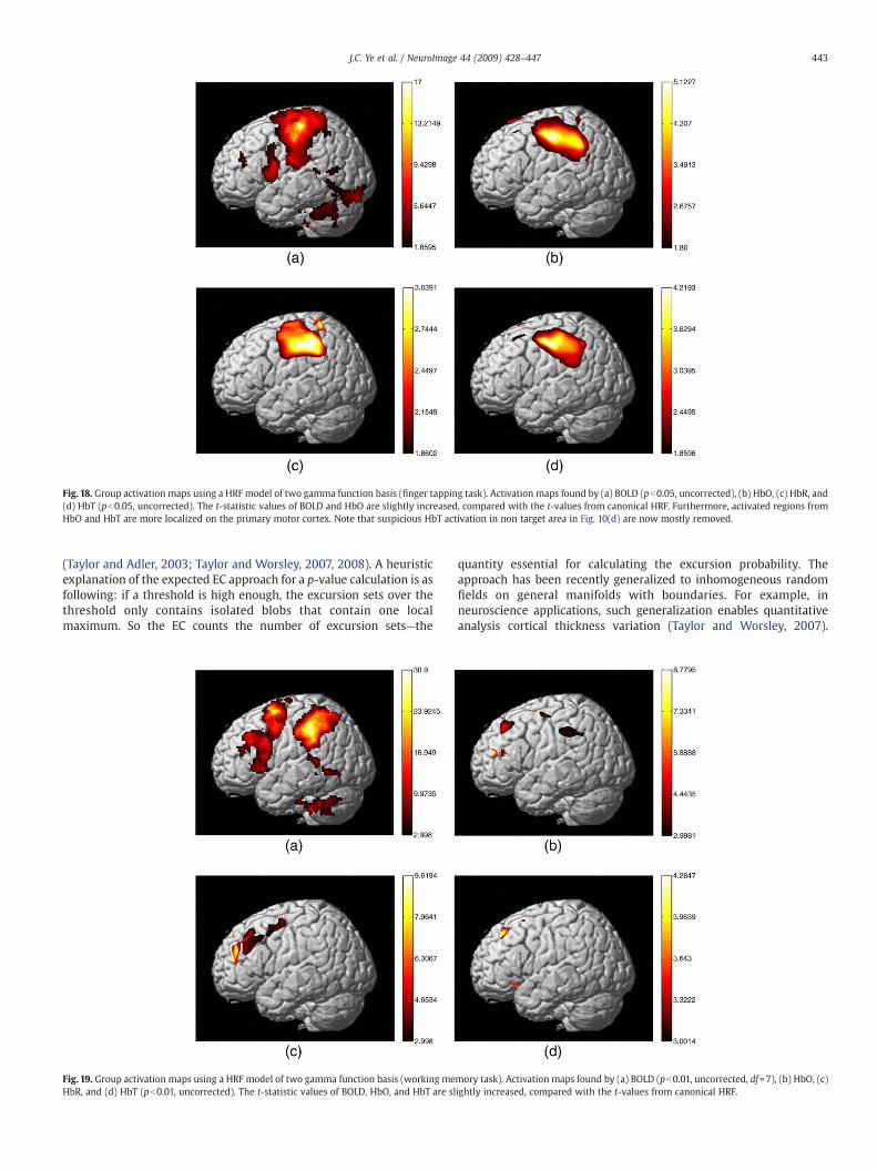
Fig. 18. Group activation maps using a HRF model of two gamma function basis (finger tapping task). Activation maps found by (a) BOLD (pb0.05, uncorrected), (b) HbO, (c) HbR, and(d) HbT (pb0.05, uncorrected). The t-statistic values of BOLD and HbO are slightly increased, compared with the t-values from canonical HRF. Furthermore, activated regions fromHbO and HbT are more localized on the primary motor cortex. Note that suspicious HbT activation in non target area in Fig. 10(d) are now mostly removed.

443J.C. Ye et al. / NeuroImage 44 (2009) 428–447

(Taylor and Adler, 2003; Taylor and Worsley, 2007, 2008). A heuristicexplanation of the expected EC approach for a p-value calculation is asfollowing: if a threshold is high enough, the excursion sets over thethreshold only contains isolated blobs that contain one localmaximum. So the EC counts the number of excursion sets—the

Fig. 19. Group activation maps using a HRF model of two gamma function basis (working meHbR, and (d) HbT (pb0.01, uncorrected). The t-statistic values of BOLD, HbO, and HbT are sl

quantity essential for calculating the excursion probability. Theapproach has been recently generalized to inhomogeneous randomfields on general manifolds with boundaries. For example, inneuroscience applications, such generalization enables quantitativeanalysis cortical thickness variation (Taylor and Worsley, 2007).

mory task). Activation maps found by (a) BOLD (pb0.01, uncorrected, df=7), (b) HbO, (c)ightly increased, compared with the t-values from canonical HRF.

444 J.C. Ye et al. / NeuroImage 44 (2009) 428–447

Currently, major statistical packages such as fMRISTAT (available athttp://www.math.mcgill.ca/keith/fmristat/) include inference enginebased on this.

The tube formula (Johansen and Johnstone, 1990; Sun, 1993; Sunand Loader, 1994) is another approach to calculate the p-value of themaximum of a random field. As described in Appendix D, the tubeformula is based on the finite expansion of Karhunen–Loeveexpansion of the random field, whose basis functions consist ofindependent zero mean unit variance Gaussian random variables.Then, the p-value of the maximum of the first m terms of theKarhunen–Loeve expansion corresponds to ratio of the measure of a“tube” to the measure of the m-dimensional unit sphere, where theradius of the tube depends on the threshold of the random field. Thetube formula does not assume any isotropy; hence, it can be applied toinhomogeneous Gaussian random fields. Furthermroe, according toTaylor and Worsley (2008), “in an unpublished manuscript by Sun, itwas generalized to include more general boundary cases”. In the caseof Gaussian random fields, Takemura and Kuriki (2002) show that thetube formula and the expected EC essentially give the same results.

The expected EC approach can be now applied to non-Gaussianrandom fields such as t- and F-statistics with the help of the union-intersection principle (Taylor and Worsley, 2008). However, theapplication of union-intersection principle to the tube formula mayappear difficult in general since the required high dimensionalembedding may complicate the Karhunen–Loeve expansion of theresultant higher dimensional random fields.

Interestingly, for the case of interpolated random fields describedin NIRS-SPM, Appendix D shows that the union-intersection trick canbe still applied to calculate the excursion probability of the t-statisticwithout altering the finiteness of Karhunen–Loeve expansion.Furthermore, p-value can be calculated directly using the close formexpression of the derivatives of the basis and the noise covariancematrix, without resorting to the mesh map as in the expected ECapproach. Hence, even though the two approaches provide theessentially same p-values, the tube formula appears easier for NIRS-SPM.

Stand-alone NIRS vs. simultaneous fMRI/NIRS

In most of the cases when noMRI record is available, onewill placethe optodes with a priori knowledge and may define ROIs based ontheir localization. Here no information of interpolation will enter thecalculated mean values.5 For these stand-alone applications, theaccurate localization property of NIRS-SPM may not be noticeablesince the exact location of the optodes are not available. However, if aseparately acquired MR image can provide the MNI coordinate of eachoptode, NIRS-SPM can still provide useful spatial information of theactivation map. Furthermore, the recent study (Tsuzuki et al., 2007)showed that the spatial registration of stand-alone NIRS data ontoMNI space without any anatomical information of MRI. If exact optodepositions in MNI space can be obtained, NIRS-SPM framework is stilluseful for obtaining the high resolution activation maps.

The effective degrees of freedom

In order to calculate the p-value of the t-statistics using Sun's tubeformula, t-statistics should be reasonably approximated by the z-score. How well the t-statistics is approximated by the z-score isdetermined by the degrees of freedom. The larger the degrees offreedom are, the better the z-approximation of the t-statistics. Asshown in Figs. 6a,b, the length of NIRS time series (NN5000) issignificantly larger than that of fMRI time series (NN183), implying

5 The authors acknowledge the anonymous reviewer who pointed out this issue.This sentence was borrowed from the comment of this reviewer.

significantly large degree of freedom. However, the existence oftemporal correlations decreases the effective degrees of freedomdefined by Eq. (23). From this perspective, the precoloring method isnot as effective as prewhitening method in providing large effectivedegrees of freedom (df=82.47 vs df=5364 for finger tapping experi-ment), since the resultant temporal correlation of precoloring ismainly dominated by the cannonical HRF filter (see Eq. (55) for theexact expression of serial correlation). However, the experimentallymeasured effective degrees of freedom by the precoloring is still in areasonable range considering that Worsley and Friston (1995)indicated the z-approximation of t-statistics is accurate as long asdfN40.

Conclusion

A new public domain statistical toolbox known as NIRS-SPM isintroduced in this study. In the main framework, NIRS-SPM success-fully analyzed NIRS data using GLM and calculated the p-value as theexcursion probability for an inhomogeneous Gaussian random fieldthat is interpolated from sparsely distributed measurements. Whenestimating the temporal correlation of NIRS, it was found that theprecoloring method is more appropriate for NIRS compared to theprewhitening method due to the sufficient temporal smoothing andcomputational efficiency of this method. In the spatial preprocess,NIRS-SPM accurately localized the NIRS signal onto the cerebral cortexof an anatomical MR image using Horn's algorithm. Experimentalresults from right finger tapping and working memory tasks showedthat the activation pattern of NIRS from the proposed softwareprogram was fairly consistent with that of fMRI. Furthermore, NIRS-SPM allowed superresolution localization of the activated area.

Acknowledgments

This research was supported by the Brain NeuroinformaticsResearch program by Korean Ministry of Knowledge Economy. Theauthors would like to thank Prof. Yong Jeong at KAIST for the valuableinput into the design of the paradigm.

Appendix A

For given wavelength λ1 and λ2, Eq. (6) can be represented by

Δ/ r; s;λ1; tð ÞΔ/ r; s;λ2; tð Þ

� �g

Rdr′

U0 r; r′;λ1ð ÞU0 r′; s;λ1ð ÞU0 r; s;λ1ð Þ Δμa r′;λ1; tð ÞR

dr′U0 r; r′;λ2ð ÞU0 r′; s;λ2ð Þ

U0 r; s;λ2ð Þ Δμa r′;λ2; tð ÞÞ

2664

3775: ð42Þ

One of the basic assumption of NIRS is that other than oxy- anddeoxy-hemoglobin variation, the optical parameters are independentof the wavelength; hence, the corresponding Green's function isidentical, i.e. U0(r,r′;λ1)=U0(r,r′;λ2). In such a case, the followingholds:

Δ/ r; s;λ1; tð ÞΔ/ r; s;λ2; tð Þ

� �g

Zdr′

U0 r; r′;λ1ð ÞU0 r′; s;λ1ð ÞU0 r; s;λ1ð Þ

Δμa r′;λ1; tð ÞΔμa r′;λ2; tð ÞÞ

� �ð43Þ

Multiplying the inverse of the extinction coefficient matrix that issimilar to Eq. (2) results in the optical density variationwith respect tothe HbX variation:

Δ/HbX r; s; tð ÞgZ

dr′U0 r; r′;λ1ð ÞU0 r′; s;λ1ð Þ

U0 r; s;λ1ð Þ ΔcHbX r′; tð Þ ð44Þ

where HbX denotes HbO or HbR. As the mapping from ΔcHbX(r′;t)to ΔϕHbX(r,s;t) is compact, stable inverse operator does not exist.If we take into consideration of the spatial correlation of adjacent

445J.C. Ye et al. / NeuroImage 44 (2009) 428–447

hemoglobin states, a regularized inverse mapping B(r′;r,s) existsand is given by:

ΔcHbX r′; tð ÞgZ Z

drds B r′; r; sð ÞΔ/HbX r; s; tð Þ ð45Þ

Given that the number of detector and source combinations isequal to the channel number K, Eq. (45) can be written in summationform:

ΔcHbX r′; tð Þg ∑K

i = 1Bi r′ð ÞΔ/HbX ri; si; tð Þ ð46Þ

where Bi(r′)=B(r′;ri,si) corresponds to the inhomogeneous interpola-tion kernel.

Appendix B

The following properties of the Kronecker product� are often used(Jain, 1989):

A� Bð ÞT = AT � BT� � ð47Þ

A� Bð Þ−1 = A−1 � B−1� �

ð48Þ

A� Bð Þ C� Dð Þ = AC� BDð Þ: ð49Þ

Then, the least-square estimation of β is given by

β^ = IK � Xð Þ†y = IK � X†� �

y ð50Þ

where X†=(XTX)−1XT denotes the pseudo-inverse of X. The corres-ponding estimation error covariance matrix is then given by

Cβ^ = E β^β^

Hi= IK � X†� �

EhyyH

iIK � X†T

� �= IK � X†� �

Ce IK � X†T� �

:h

ð51Þ

In an estimation of the error covariance matrix, SPM assumes thatthe temporal correlation matrix is identical at all voxels, but thevariance is different (Friston et al., 2006). Hence, the error covariancematrix at the ith channel is given by:

Ce ið Þ = E e ið Þe ið ÞTh i

= σ ið Þ� �2

Λ ð52Þ

where Λ is the temporal correlation matrix and (σ(i))2 denotes thevariance, respectively. The variance (σ(i))2 at the ith channel can beestimated using the usual estimator in a least squares mass-univariatescheme:

σ ið Þ� �2

=y ið ÞTRy ið Þ

trace RΛð Þ ; ð53Þ

where R= I−X(XTX)−1XT is the residual forming matrix (Worsley andFriston, 1995).

Based on this model, the following holds:

Ce =

σ 1ð Þ2Λ O : : : OO σ 2ð Þ2Λ : : : Ov v O vO O : : : σ Kð Þ2Λ

2664

3775 =∑� Λ ð54Þ

where

∑ =

σ 1ð Þ2 O : : : OO σ 2ð Þ2 : : : Ov v O vO O : : : σ Kð Þ2

2664

3775 ð55Þ

Therefore, the final form of the error covariance matrix is given by

Cβ^= IK � X†� �

∑� Λð Þ IK � X†T� �

=∑� X†ΛX†T� �

ð56Þ

Appendix C

In this section, the GLM model is derived for ΔcHbX(r;t) in Eq. (46).Stacking {ΔcHbX(r;ti)}i =1N into a vector ΔcHbX(r) gives the following:

ΔcHbX rð Þ = b rð ÞT�IN

� �y : ð57Þ

Here, b(r) denotes the basis vector given in Eq. (17) and y is givenby Eq. (11), respectively. The GLM model is then given by

ΔcHbχ rð Þ = b rð ÞT�IN

� �y = IK � Xð Þα rð Þ + e : ð58Þ

Then, with the property of the Kronecker delta product, thefollowing is true:

α̂ rð Þ = bT � X†� �

ΔcHbX rð Þ = bT � IN� �

IK � X†� �

ΔcHbX rð Þ = b rð ÞT�IN

� �β^

ð59Þ

This implies that the response signal strength for the interpolatedmeasurement is equivalent to the interpolated response signalstrength with the same interpolation kernel. Similarly, it is possibleto obtain the error covariance matrix for α̂:

Cα̂= b rð ÞT�IN

� �C

β^ b� INð Þ

= b rð ÞT∑b rð ÞT� �

� X†ΛX†T� �

: ð60Þ

Appendix D

Here, the p-value of the t-statistics to abandon null hypothesis isgiven by:

p = P maxraW

T rð Þzzn o

=12P max

raWjT rð Þj2zz2

n oð61Þ

due to the symmetry of the T(r) around zero. Furthermore, thefollowing equalities hold:

P maxraW

jT rð Þj2zz2n o

= P maxraW

cT α̂ rð Þ� �T

Cχ rð Þ−1 cT α̂ rð Þ� �

zz2 �

= P maxraW

β^TB rð Þ B rð ÞTCβ^B rð Þ

� �−1B rð ÞTβ^zz2

�

= P maxraW

ZTC1=2

β^ B rð Þ B rð ÞTC

β^B rð Þ

� �−1B rð ÞTC1=2

β^ Zzz2

�

= P maxraW

ZTP rð ÞZzz2n o

ð62Þ

where

BJcT b rð ÞT�IN

� �

ZJC−1=2

β^ βaR

KM

ð63Þ

P rð ÞJC1=2

β^ B rð Þ BT rð ÞC

β^ B rð Þ

� �−1BT rð ÞC1=2

β^ ð64Þ

where ZfN O; IKMð Þ denotes the zero-mean independent Gaussianrandom vector and P(r) is the KM×KM projection matrix onto therange space of C1=2

β^ B rð Þ, which is well defined for all r∈Ψ. Hence,

using Eqs. (19) and (20), the following decomposition holds true:

P rð Þ = u rð Þu rð ÞT : ð65Þ

446 J.C. Ye et al. / NeuroImage 44 (2009) 428–447

The unit vector u in this case is given by

u =C

1=2

β^;HbO2

b rð ÞT�IM

� �c

ffiffiffiffiffiffiffiffiffiffiffiffiffiffiffiffiffiffiffiffiffiffiffiffiffiffiffiffiffiffib rð ÞT∑b rð Þ

� �r ffiffiffiffiffiffiffiffiffiffiffiffiffiffiffiffiffiffiffiffiffiffiffiffiffiffiffiffifficTX†ΛX†Tc

� �r ð66Þ

The excursion probability in Eq. (62) can be calculated using theexcursion probability of the zero-mean unit variance inhomogeneousGaussian random field:

p =12P max

raWZTP rð ÞZzz2

n o= P max

raWχ rð Þzz

n o: ð67Þ

where the excursion probability of an non-Gaussian random field canbe converted into a Gaussian random field using the similar techniquein Taylor and Worsley (2008):

χ rð Þ = u rð ÞHZ : ð68Þ

At this point, inhomogeneous Gaussian random field theory suchas expected EC (Taylor and Adler, 2003; Taylor and Worsley, 2007,2008) or tube formula (Sun, 1993; Cao and Worsley, 1999b) can beapplied to calculate the p-value. In this paper, we prefer the tubeformula thanks to the finite Karhunen–Loève expansion of theresultant covariance matrix.

More specifically, a case in which Ψ is a compact subset of ℝN andX(r), r∈Ψ is a non-singular Gaussian random field with zero mean,unit variance, and covariance function CX(r,r′) is considered. If CX(r,r′)has finite Karhunen–Loève expansion

Cχ r; r′ð Þ = ∑M

i = 1ui rð Þui r′ð Þ; ð69Þ

and the manifold U={[ui(r),⋯,uM(r)]T, r∈Ψ} has no boundary, then

P supraW

χ rð Þzz �

= κ0ψ0 zð Þ +: : : + κ D̃ψD̃ βð Þ + o ψD̃ zð Þ� � ð70Þ

where D̃=D for an even value of D and D̃=D−1 for an odd value of D,respectively. Here

ψn zð Þ = 1

21 + n=2π D + 1ð Þ=2

Z ∞

z2=2u D + 1−nð Þ=2−1e−udu ; ð71Þ

where n = 0;2;: : :;D~. In Eq. (70), κ0;: : :; κD

~ are the constants in Weyl'sformula (Weyl, 1939) for the manifold U.

Interestingly, the covariance matrix for Eq. (68) can be simplyrepresented as a finite Karhunen–Loève expansion:

Cχ r; r′ð Þ = ∑KM

i = 1ui rð Þui r′ð Þ ð72Þ

where ui(r) denotes the i-th elements of u rð ÞaℝKM . Therefore, Sun'stube formula can be utilized. While κ0;: : :κ D̃ are important constantsfromWeyl's formula, the most important constant to calculate simplyis κ0. This constant is related to the metric tensor of the manifold U:

R rð ÞJE jχ rð ÞjTχ rð Þ� � ð73Þ

and

κ0 = jUj =ZW

ffiffiffiffiffiffiffiffiffiffiffiffiffiffiffiffiffiffiffiffiffiffiffiffijdet R rð Þð Þj

qdr ð74Þ

Therefore, the p-value for the activation map can be approximatedby

p = P maxraWT rð Þzzf gg κ0

ωD1−Γ

D + 12

;z2

2

1 +O z−2

� �� � ð75Þ

where κ0 is given by Eq. (74) and

ωD =2π D + 1ð Þ=2

C D + 12

� � ð76Þ

denotes the surface area of the (D+1)-dimensional unit sphere, andthe incomplete Gamma function as

C a;χð Þ = 1C að Þ

Z χ

0e−yya−1dy; aaℝ; χz0: ð77Þ

Here,C 1=2ð Þ = ffiffiffiπ

pand Γ(a+1)=aΓ(a). Using the asymptotic formula

for the incomplete gamma function

1−Γ a;χð Þ˜1

Γ að Þχa−1e−χ as χ→∞: ð78Þ

for D=3 the following equation can be derived:

pfκ0

2πð Þ2z2exp −

z2

2

: ð79Þ

This implies that the present formula is an extension of thehomogenous Gaussian random field formula due to the equalityκ0=V|Λ|−1/2 for homogeneous Gaussian random field, where V is thevolume and Λ denotes the 3×3 variance matrix of the partialderivatives of the underlying Gaussian random field.

In real measurement scenario, the interpolation function Bi(r) isthree-dimensional, i.e. Woℝ3 and D=3. However, the NIRS optodecoverage is on a two dimensional manifold and the representationover the fMRI map has to be two dimensional. Hence, the twodimensional interpolation function is sufficient to represent theinterpolated NIRS signals. Therefore, the resultant random field isassumed two dimensional.

References

Adler, R.J., 1981. The Geometry of Random Fields. John Wiley & Sons, New York.Adler, R.J., 2000. On excursion sets, tube formulae, and maxima of random fields. Ann.

Appl. Probab. 10 (1), 1–74.Adler, R., Taylor, J., 2007. Random Fields and Geometry. Springer, New York.Beckmann, C., Jenkinson, M., Smith, S., 2003. General multilevel linear modeling for

group analysis in fMRI. NeuroImage 20 (2), 1052–1063.Benaron, D., Hintz, S., Villringer, A., Boas, D., Kleinschmidt, A., Frahm, J., Hirth, C., Obrig,

H., van Houten, J., Kermit, E., et al., 2000. Noninvasive functional imaging of humanbrain using light. J. Cereb. Blood Flow Metab. 20, 469–477.

Boas, D.A., O'Leary, M.A., Chance, B., Yodh, A.G., July 1997. Detection and characteriza-tion of optical inhomogeneities with diffuse photon density waves: a signal-to-noise analysis. Appl. Opt. 36, 75–92.

Boas, D., Brooks, D., Miller, E., DiMarzio, C., Kilmer, M., Gaudette, R., 2001. Imaging thebody with diffuse optical tomography. IEEE Signal Process. Mag. 18 (6), 57–75.

Boas, D., Strangman, G., Culver, J., Hoge, R., Jasdzewski, G., Poldrack, R., Rosen, B.,Mandeville, J., 2003. Can the cerebral metabolic rate of oxygen be estimated withnear-infrared spectroscopy? Phys. Med. Biol. 48 (15), 2405–2418.

Boas, D., Dale, A., Franceschini, M., 2004. Diffuse optical imaging of brain activation:approaches to optimizing image sensitivity, resolution, and accuracy. NeuroImage23, 275–288.

Bullmore, E., Brammer, M., Williams, S.C., Rabe-Hesketh, S., Janot, N., David, A., Mellers,J., Howard, R., Sham, P., 1996. Statistical methods of estimation and inference forfunctional MR image analysis. Magn. Reson. Med. 35, 261–277.

Cannestra, A., Pouratian, N., Bookheimer, S., Martin, N., Becker, D., Toga, A., 2001.Temporal spatial differences observed by functional MRI and human intraoperativeoptical imaging. Cereb. Cortex 11 (8), 773–782.

Cao, J., Worsley, K., 1999a. The detection of local shape changes via the geometry ofHotellings T2 fields. Ann. Stat. 27 (3), 925–942.

Cao, J., Worsley, K., 1999b. The geometry of the Hotelling's random field withapplications to the detection of shape changes. Ann. Stat. 27 (3), 925–942.

Chen, Y., Tailor, D., Intes, X., Chance, B., 2003. Correlation between near-infraredspectroscopy and magnetic resonance imaging of rat brain oxygenation modula-tion. Phys. Med. Biol. 48 (4), 417–427.

Cope, M., Delpy, D.T., May 1988. System for long-term measurement of cerebral bloodand tissue oxygenation on newborn infants by near infra-red transillumination.Med. Biol. Eng. Comput. 26, 289–294.

Friston, K.J., Holmes, A.P., Poline, J.B., Price, C.J., Frith, C.D., December 1996. Detectingactivations in PET and fMRI: levels of inference and power. NeuroImage 40,223–235.

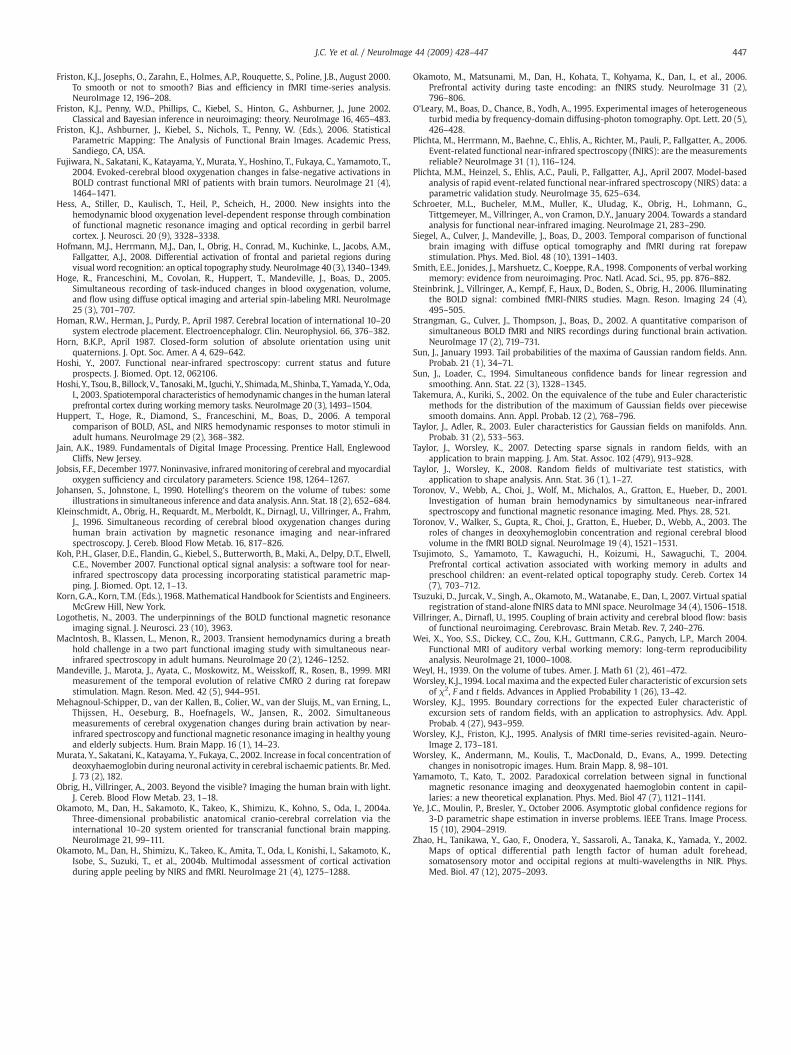
447J.C. Ye et al. / NeuroImage 44 (2009) 428–447

Friston, K.J., Josephs, O., Zarahn, E., Holmes, A.P., Rouquette, S., Poline, J.B., August 2000.To smooth or not to smooth? Bias and efficiency in fMRI time-series analysis.NeuroImage 12, 196–208.

Friston, K.J., Penny, W.D., Phillips, C., Kiebel, S., Hinton, G., Ashburner, J., June 2002.Classical and Bayesian inference in neuroimaging: theory. NeuroImage 16, 465–483.

Friston, K.J., Ashburner, J., Kiebel, S., Nichols, T., Penny, W. (Eds.), 2006. StatisticalParametric Mapping: The Analysis of Functional Brain Images. Academic Press,Sandiego, CA, USA.

Fujiwara, N., Sakatani, K., Katayama, Y., Murata, Y., Hoshino, T., Fukaya, C., Yamamoto, T.,2004. Evoked-cerebral blood oxygenation changes in false-negative activations inBOLD contrast functional MRI of patients with brain tumors. NeuroImage 21 (4),1464–1471.

Hess, A., Stiller, D., Kaulisch, T., Heil, P., Scheich, H., 2000. New insights into thehemodynamic blood oxygenation level-dependent response through combinationof functional magnetic resonance imaging and optical recording in gerbil barrelcortex. J. Neurosci. 20 (9), 3328–3338.

Hofmann, M.J., Herrmann, M.J., Dan, I., Obrig, H., Conrad, M., Kuchinke, L., Jacobs, A.M.,Fallgatter, A.J., 2008. Differential activation of frontal and parietal regions duringvisual word recognition: an optical topography study. NeuroImage 40 (3),1340–1349.

Hoge, R., Franceschini, M., Covolan, R., Huppert, T., Mandeville, J., Boas, D., 2005.Simultaneous recording of task-induced changes in blood oxygenation, volume,and flow using diffuse optical imaging and arterial spin-labeling MRI. NeuroImage25 (3), 701–707.

Homan, R.W., Herman, J., Purdy, P., April 1987. Cerebral location of international 10–20system electrode placement. Electroencephalogr. Clin. Neurophysiol. 66, 376–382.

Horn, B.K.P., April 1987. Closed-form solution of absolute orientation using unitquaternions. J. Opt. Soc. Amer. A 4, 629–642.

Hoshi, Y., 2007. Functional near-infrared spectroscopy: current status and futureprospects. J. Biomed. Opt. 12, 062106.

Hoshi, Y., Tsou, B., Billock,V., Tanosaki,M., Iguchi, Y., Shimada,M., Shinba, T., Yamada, Y., Oda,I., 2003. Spatiotemporal characteristics of hemodynamic changes in the human lateralprefrontal cortex during working memory tasks. NeuroImage 20 (3), 1493–1504.

Huppert, T., Hoge, R., Diamond, S., Franceschini, M., Boas, D., 2006. A temporalcomparison of BOLD, ASL, and NIRS hemodynamic responses to motor stimuli inadult humans. NeuroImage 29 (2), 368–382.

Jain, A.K., 1989. Fundamentals of Digital Image Processing. Prentice Hall, EnglewoodCliffs, New Jersey.

Jobsis, F.F., December 1977. Noninvasive, infraredmonitoring of cerebral andmyocardialoxygen sufficiency and circulatory parameters. Science 198, 1264–1267.

Johansen, S., Johnstone, I., 1990. Hotelling's theorem on the volume of tubes: someillustrations in simultaneous inference and data analysis. Ann. Stat. 18 (2), 652–684.

Kleinschmidt, A., Obrig, H., Requardt, M., Merboldt, K., Dirnagl, U., Villringer, A., Frahm,J., 1996. Simultaneous recording of cerebral blood oxygenation changes duringhuman brain activation by magnetic resonance imaging and near-infraredspectroscopy. J. Cereb. Blood Flow Metab. 16, 817–826.

Koh, P.H., Glaser, D.E., Flandin, G., Kiebel, S., Butterworth, B., Maki, A., Delpy, D.T., Elwell,C.E., November 2007. Functional optical signal analysis: a software tool for near-infrared spectroscopy data processing incorporating statistical parametric map-ping. J. Biomed. Opt. 12, 1–13.

Korn, G.A., Korn, T.M. (Eds.), 1968. Mathematical Handbook for Scientists and Engineers.McGrew Hill, New York.

Logothetis, N., 2003. The underpinnings of the BOLD functional magnetic resonanceimaging signal. J. Neurosci. 23 (10), 3963.

MacIntosh, B., Klassen, L., Menon, R., 2003. Transient hemodynamics during a breathhold challenge in a two part functional imaging study with simultaneous near-infrared spectroscopy in adult humans. NeuroImage 20 (2), 1246–1252.

Mandeville, J., Marota, J., Ayata, C., Moskowitz, M., Weisskoff, R., Rosen, B., 1999. MRImeasurement of the temporal evolution of relative CMRO 2 during rat forepawstimulation. Magn. Reson. Med. 42 (5), 944–951.

Mehagnoul-Schipper, D., van der Kallen, B., Colier, W., van der Sluijs, M., van Erning, L.,Thijssen, H., Oeseburg, B., Hoefnagels, W., Jansen, R., 2002. Simultaneousmeasurements of cerebral oxygenation changes during brain activation by near-infrared spectroscopy and functional magnetic resonance imaging in healthy youngand elderly subjects. Hum. Brain Mapp. 16 (1), 14–23.

Murata, Y., Sakatani, K., Katayama, Y., Fukaya, C., 2002. Increase in focal concentration ofdeoxyhaemoglobin during neuronal activity in cerebral ischaemic patients. Br. Med.J. 73 (2), 182.

Obrig, H., Villringer, A., 2003. Beyond the visible? Imaging the human brain with light.J. Cereb. Blood Flow Metab. 23, 1–18.

Okamoto, M., Dan, H., Sakamoto, K., Takeo, K., Shimizu, K., Kohno, S., Oda, I., 2004a.Three-dimensional probabilistic anatomical cranio-cerebral correlation via theinternational 10–20 system oriented for transcranial functional brain mapping.NeuroImage 21, 99–111.

Okamoto, M., Dan, H., Shimizu, K., Takeo, K., Amita, T., Oda, I., Konishi, I., Sakamoto, K.,Isobe, S., Suzuki, T., et al., 2004b. Multimodal assessment of cortical activationduring apple peeling by NIRS and fMRI. NeuroImage 21 (4), 1275–1288.

Okamoto, M., Matsunami, M., Dan, H., Kohata, T., Kohyama, K., Dan, I., et al., 2006.Prefrontal activity during taste encoding: an fNIRS study. NeuroImage 31 (2),796–806.

O'Leary, M., Boas, D., Chance, B., Yodh, A., 1995. Experimental images of heterogeneousturbid media by frequency-domain diffusing-photon tomography. Opt. Lett. 20 (5),426–428.

Plichta, M., Herrmann, M., Baehne, C., Ehlis, A., Richter, M., Pauli, P., Fallgatter, A., 2006.Event-related functional near-infrared spectroscopy (fNIRS): are the measurementsreliable? NeuroImage 31 (1), 116–124.

Plichta, M.M., Heinzel, S., Ehlis, A.C., Pauli, P., Fallgatter, A.J., April 2007. Model-basedanalysis of rapid event-related functional near-infrared spectroscopy (NIRS) data: aparametric validation study. NeuroImage 35, 625–634.

Schroeter, M.L., Bucheler, M.M., Muller, K., Uludag, K., Obrig, H., Lohmann, G.,Tittgemeyer, M., Villringer, A., von Cramon, D.Y., January 2004. Towards a standardanalysis for functional near-infrared imaging. NeuroImage 21, 283–290.

Siegel, A., Culver, J., Mandeville, J., Boas, D., 2003. Temporal comparison of functionalbrain imaging with diffuse optical tomography and fMRI during rat forepawstimulation. Phys. Med. Biol. 48 (10), 1391–1403.

Smith, E.E., Jonides, J., Marshuetz, C., Koeppe, R.A., 1998. Components of verbal workingmemory: evidence from neuroimaging. Proc. Natl. Acad. Sci., 95, pp. 876–882.

Steinbrink, J., Villringer, A., Kempf, F., Haux, D., Boden, S., Obrig, H., 2006. Illuminatingthe BOLD signal: combined fMRI-fNIRS studies. Magn. Reson. Imaging 24 (4),495–505.

Strangman, G., Culver, J., Thompson, J., Boas, D., 2002. A quantitative comparison ofsimultaneous BOLD fMRI and NIRS recordings during functional brain activation.NeuroImage 17 (2), 719–731.

Sun, J., January 1993. Tail probabilities of the maxima of Gaussian random fields. Ann.Probab. 21 (1), 34–71.

Sun, J., Loader, C., 1994. Simultaneous confidence bands for linear regression andsmoothing. Ann. Stat. 22 (3), 1328–1345.

Takemura, A., Kuriki, S., 2002. On the equivalence of the tube and Euler characteristicmethods for the distribution of the maximum of Gaussian fields over piecewisesmooth domains. Ann. Appl. Probab. 12 (2), 768–796.

Taylor, J., Adler, R., 2003. Euler characteristics for Gaussian fields on manifolds. Ann.Probab. 31 (2), 533–563.

Taylor, J., Worsley, K., 2007. Detecting sparse signals in random fields, with anapplication to brain mapping. J. Am. Stat. Assoc. 102 (479), 913–928.

Taylor, J., Worsley, K., 2008. Random fields of multivariate test statistics, withapplication to shape analysis. Ann. Stat. 36 (1), 1–27.

Toronov, V., Webb, A., Choi, J., Wolf, M., Michalos, A., Gratton, E., Hueber, D., 2001.Investigation of human brain hemodynamics by simultaneous near-infraredspectroscopy and functional magnetic resonance imaging. Med. Phys. 28, 521.

Toronov, V., Walker, S., Gupta, R., Choi, J., Gratton, E., Hueber, D., Webb, A., 2003. Theroles of changes in deoxyhemoglobin concentration and regional cerebral bloodvolume in the fMRI BOLD signal. NeuroImage 19 (4), 1521–1531.

Tsujimoto, S., Yamamoto, T., Kawaguchi, H., Koizumi, H., Sawaguchi, T., 2004.Prefrontal cortical activation associated with working memory in adults andpreschool children: an event-related optical topography study. Cereb. Cortex 14(7), 703–712.

Tsuzuki, D., Jurcak, V., Singh, A., Okamoto, M., Watanabe, E., Dan, I., 2007. Virtual spatialregistration of stand-alone fNIRS data to MNI space. NeuroImage 34 (4), 1506–1518.

Villringer, A., Dirnafl, U., 1995. Coupling of brain activity and cerebral blood flow: basisof functional neuroimaging. Cerebrovasc. Brain Metab. Rev. 7, 240–276.

Wei, X., Yoo, S.S., Dickey, C.C., Zou, K.H., Guttmann, C.R.G., Panych, L.P., March 2004.Functional MRI of auditory verbal working memory: long-term reproducibilityanalysis. NeuroImage 21, 1000–1008.

Weyl, H., 1939. On the volume of tubes. Amer. J. Math 61 (2), 461–472.Worsley, K.J., 1994. Local maxima and the expected Euler characteristic of excursion sets

of χ2, F and t fields. Advances in Applied Probability 1 (26), 13–42.Worsley, K.J., 1995. Boundary corrections for the expected Euler characteristic of

excursion sets of random fields, with an application to astrophysics. Adv. Appl.Probab. 4 (27), 943–959.

Worsley, K.J., Friston, K.J., 1995. Analysis of fMRI time-series revisited-again. Neuro-Image 2, 173–181.

Worsley, K., Andermann, M., Koulis, T., MacDonald, D., Evans, A., 1999. Detectingchanges in nonisotropic images. Hum. Brain Mapp. 8, 98–101.

Yamamoto, T., Kato, T., 2002. Paradoxical correlation between signal in functionalmagnetic resonance imaging and deoxygenated haemoglobin content in capil-laries: a new theoretical explanation. Phys. Med. Biol 47 (7), 1121–1141.

Ye, J.C., Moulin, P., Bresler, Y., October 2006. Asymptotic global confidence regions for3-D parametric shape estimation in inverse problems. IEEE Trans. Image Process.15 (10), 2904–2919.

Zhao, H., Tanikawa, Y., Gao, F., Onodera, Y., Sassaroli, A., Tanaka, K., Yamada, Y., 2002.Maps of optical differential path length factor of human adult forehead,somatosensory motor and occipital regions at multi-wavelengths in NIR. Phys.Med. Biol. 47 (12), 2075–2093.