nina siu-ngan lam nasa - louisiana state · pdf filenina siu-ngan lam department of geography...

NINA SIU-NGAN LAMDepartment of GeograPhy and Anthropology

Louisiana State UniversityBaton Rouge, Louisiana 70803

DALE QUATTROCHINASA

Global Hydrology and Climate CenterMarshall Space Flight CenterHuntsville, Alabama 35812

HONG-LIE QIU

Department of GeograPhyCalifornia State University, Los Angeles

Los Angeles, California 90032

WEI ZHAODepartment of Geography and Anthropology

Louisiana State UniversityBaton Rouge, Louisiana 70803

Received October 1996; accepted October 1997

With the rapid increase in spatial data, especially in the NASA-EOS (Earth ObservingSystem) era, it is necessary to develop efficient and innovative tools to handle andanalyze these data so that environmental conditions can be assessed and monitored. Amain difficulty facing geographers and environmental scientists in environmental assess-

Acknowledgments: This research is supported by a research grant from NASA (Award No. NAGW-4221). Weappreciate the comments of the anonymous reviewers.Reprint requests should be directed to: Nina Siu-Ngan Lam.

APPLIED GEOGRAPHIC STUDIES, Vol. 2, No.2, 77-93@ 1998 by John Wiley & Sons, Inc. CCC 1083-3404/98/020077-17

Lam et al.

ment and measurement is that spatial analytical tools are not easily accessible. We haverecently developed a remote sensing/GIS software module called ICAMS (Image Char-acterization And Modeling System) to provide specialized spatial analytical tools forthe measurement and characterization of satellite and other forms of spatial data.ICAMS runs on both the Intergraph-MGE and the Arc/Info Unix and Windows-NTplatforms. The main techniques in ICAMS include fractal measurement methods,variogram analysis, spatial autocorrelation statistics, textural measures, aggregationtechniques, normalized difference vegetation index (NDVI), and delineation of land/water and vegetated/non-vegetated boundaries. In this article, we demonstrate themain applications of ICAMS on the Intergraph-MGE platform using Landsat-Thematic Mapper images from the city of Lake Charles, Louisiana. Through theavailability of ICAMS to a wider scientific community, we hope to generate variousstudies so that improved algorithms and more reliable models for environmentalassessment and monitoring can be developed. @ 1998 john Wiley & Sons, Inc.

INTRODUCTION

The use of remote sensing data in global environmental modeling studies has grownrapidly in the last decade, owing largely to the increasing availability of these and othertypes of spatial data in digital form at global, regional, and local scales, from manysources. The National Aeronautics and Space Administration's Earth Observing System(NASA-EOS) initiative, to be launched late in this century, will add a plethora of spatialdata that will help in more effectively assessing environmental conditions and managingnatural resources. The fast pace of increase in digital data, however, presents an imme-diate problem, that is, how these data can be handled and analyzed efficiently (justiceet al., 1995). Advances in environmental monitoring and assessment require three com-ponents. In addition to high-quality data sets, we need reliable tools to handle andanalyze these data sets, and such tools must be made available to the research andpolicy-making communities.

The current state of environmental research recognizes that the Earth's environmentis so complex that it is difficult, if not impossible, to understand all of its processes. Yetan understanding of all the processes i~ needed to formulate effective environmentalpolicies. Among the problems involved in environmental modeling is that researchersare often impaired by the lack of analytical tools to analyze remote sensing data. Geo-graphic information systems (GIS) and quantitative models offer an attractive set oftechniques for environmental modeling and are increasingly recognized as a vital part ofresearch in resource management, environmental risk assessment, and global monitor-ing and modeling. Integration of environmental modeling and spatial tech~iques isconsidered a top research priority, and in order to make full use of available digital datafor effective environmental research the immediate need is to develop user-friendlycomputer systems that include useful spatial analytical functions for high-quality data(Goodchild et al., 1993).

An integral part of understanding earth processes as a system is to understand howto combine data with different spatial and temporal properties in a meaningful way. Thistype of multiscale data integration and modeling is a necessary component in environ-mental research, as environmental and ecological phenomena are scale dependent innature. Quattrochi and Goodchild (1997) documented some of the more importantscale issues in remote sensing and GIS. For example, one of the basic goals of land-atmospheric interaction modeling research is to be able to move up and down the spatialscales so that the results at one scale can be inferred to another scale (Kineman, 1993;

78 Vol. 2, No.2

Environmental Assessment and Monitoring

Steyaert, 1993; Townshend and Justice, 1988; Turner et al., 1989a, 1989b). Extrapolationof results across broad spatial scales remains the most difficult problem in global envi-ronmental research. Many methods have been suggested to tackle the scale and resolu-tion problem. Whichever method is used, we believe that basic characterization andparameterization of image data is a prerequisite, and techniques for measuring scaleeffects must be developed and implemented to allow for a multiscale assessment of thesedata before any usefu. process-oriented modeling involving scale-dependent data can bemade.

We have recently developed a data characterization and analysis GIS module calledICAMS (Image Characterization And Modeling System) to address two of the threefollowing components: the research and development of innovative spatial analytical andmeasurement tools for characterizing multiscale remote sensing data, and the bundlingof these measurement tools into an integrated, user-friendly, interactive module for easyaccess by the general scientific community. This article presents some of the initialresults of the ICAMS project. A brief description of the design principles and functionsof ICAMS, with a focus on the Intergraph-MGE platform, is first provided. Using twoLandsat-Thematic Mapper (TM) images from the city of Lake Charles, Louisiana, wedemonstrate the functionality of ICAMS in characterizing and measuring remote sensingimages. Interpretations of the resultant indices and boundaries are presented, and sug-gestions are then made on how they can be used in assessing and monitoring environ-mental conditions.

THE ICAMS MODULE

A description of an earlier version of ICAMS on the Arc/Info platform can be found inQuattrochi, Lam, et al. (1997). In the following, we highlight the software objectives,design principles, and main functions of ICAMS, and demonstrate example applicationswith the use of ICAMS on the Intergraph-MGE platform. It should be noted that thesame algorithms have been implemented on both Intergraph-MGE and Arc/Info plat-forms, but because each system has its own display and system requirements, the graphicdisplays and procedures to run ICAMS may be different.

Objectives and Design Principles

lCAMS is designed to provide scientists with innovative spatial analytical tools to visual-ize, measure, and characterize landscape patterns so that environmental conditions orprocesses can be assessed and monitored more effectively. In developing lCAMS, weemphasize three design elements: interactive, integrative, and innovative (the three Is).Our primary goal is to provide specialized image characterization functions, such asfractal analysis, variogram analysis, and multiscale analysis, that are not easily available incommercial GIS software. Also, we have developed lCAMS as a module compatible withthe two most widely used GIS software, Intergraph-MGE and Arc/Info, instead of devel-oping it on a generic, stand-alone platform. Also, Arc/Info has a link with anotheradvanced image processing software-ERDAS/lMAGINE. The advantages of building amodule on these two commercial GIS platforms are twofold. First, using these platformswe can utilize most of the basic image input, output, and interface functions such as filetransfers, image displays, and image outputs, without the need to re-program these basicfunctions from ground zero. This minimizes duplication and ensures that the specializedfunctions in lCAMS can be made available within a shorter time frame by circumventing

APPLIED GEOGRAPHIC STUDIES 79

Lam et ai.

extensive and time-consuming software development. Second, because these platformshave been widely used, a specialized module designed to be compatible with thesesystems will encourage a wider access of ICAMS.

Main Functions

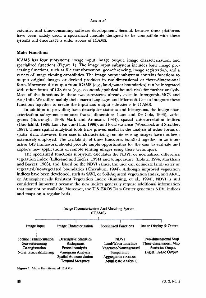
ICAMS has four subsystems: image input, image output, image characterization, andspecialized functions (Figure 1). The image input subsystem includes basic image pro-cessing functions, such as file transformation, georeferencing, image registration, and avariety of image viewing capabilities. The image output subsystem contains functions tooutput original images or derived products in two-dimensional or three-dimensionalform. Moreover, the output from ICAMS (e.g., land/water boundaries) can be integratedwith other forms of GIS data (e.g., economic/political boundaries) for further analysis.Most of the functions in these two subsystems already exist in Intergraph-MGE andArc/Info. We utilize mainly their macro languages and Microsoft C++ to integrate thesefunctions together to create the input and output subsystems in ICAMS.

In addition to providing basic descriptive statistics and histograms, the image char-acterization subsystem computes fractal dimensions (Lam and De Cola, 1993), vario-grams (Burrough, 1993; Mark and Aronson, 1984), spatial autocorrelation indices(Goodchild, 1986; Lam, Fan, and Liu, 1996), and local variance (Woodcock and Strahler,1987). These spatial analytical tools have proved useful in the analysis of other forms ofspatial data. However, their uses in characterizing remote sensing images have not beenextensively employed. The availability of these functions, bundled together in an inter-active GIS framework, should provide ample opportunities for the user to evaluate andexplore new applications of remote sensing images using these techniques.

The specialized functions subsystem calculates the NDVI, or normalized differencevegetation index (Lillesand and Kiefer, 1994) and temperature (Lobitz, 1994; Markhamand Barker, 1986), and, based on the NDVI values, the user can delineate land/water orvegetated/nonvegetated boundaries (Cherukuri, 1994). Although improved vegetationindices have been developed, such as SAVI, or Soil-Adjusted Vegetation Index, and ARVI,or Atmospherically Resistant Vegetation Index (Running, et al., 1994), NDVI is stillconsidered important because the new indices generally require additional informationthat may not be available. Moreover, the u.S. EROS Data Center generates NDVI indicesand maps on a regular basis.

Image Characterization And Modeling System(ICAMS)

Image Input

IFonIlat Transformation

Geo-referencingCo-registration

Noise removal/filtering

Image: Display & OutputImage ChaIa(:terization Specialized Functions

Descriptive StatisticsHistograms

Fractal AnalysisVariogram Analysis

Spatial AutocorrelationTextural Mleasures

Twc>-dimensional MapThree-dimensional Map

Statistics OutputDi!~tal Image Output

NDVILand/Water Interfaa~

Vegetated/N onvegeta1:ed

Aggregation routines(Multi scale Analysi~:)

Figure 1 Main functions of ICAMS.

Vol. 2, No.280


An aggregation function is provided to resample the image according to a filter sizespecified by the user. The aggregation function currently implemented is simply anaveraging/smoothing function. It computes the average of all the pixels within a filterand replaces the filter with the average value. The aggregated image can be applied tothe image characterization subsystem again to re-compute fractal dimensions, NDVI, ortemperature, or redefine the land/water interface boundaries to evaluate the scaleeffects on indices and boundaries. The changes in these index values with scale (resam-pled image) will reveal the basic structure of the phenomena as manifested by the imageand uncertainties in measurement due to scale. This information will be useful to theformulation of more accurate global environmental models, particularly those applied atmultiple spatial scales.

AN APPliCATION

Study Area

Landsat-TM images acquired on two different dates from Lake Charles, Louisiana, areused to demonstrate some of the functions of ICAMS. Lake Charles had a population ofabout 75,000 in 1980, which decreased to 71,000 in 1992. The first image was acquiredon November 30, 1984, and the second on February 8, 19~)3. Subsets of a 5-km x 5-kmarea with a pixel resolution of 25-m x 25-m were created, with each subset containing201 x 201 pixels. Because the pixel size of the 1984 image was fixed to 25 m, the 1993image that was provided by EOSAT at approximately 28 ill was resampled to the samesize, to enhance comparison. The subsets cover part of Lake Charles. The 1984 subsethas been used as a representative urban landscape in a previous study that examines thefractal properties of remote sensing images (Lam, 1990). The selection of the same studyarea for the present study is based on the availability of data on two dates, so that analysisof temporal changes can be made. At the same time, we realize that the study area coversa medium-size urban area with little urban growth; therefore, significant changes interms of land cover are not expected in this region between these two dates.

Figure 2 displays two images using bands 2 (blue), 3 (green), and 4 (red). Althoughlarge changes in land cover were not expected, a visual comparison between the twoimages shows that the 1993 image has slightly more roads and buildings, especially in thesoutheast corner and along the highway (Highway 210) in the southern part of theimage. Table 1 lists the summary statistics of all seven bands for the two images. Withthe exception of the thermal band (band 6), the 1993 image generally has smaller rangesof spectral reflectance values, lower maximum values, and smaller coefficients of varia-tion. Although these two Landsat images were not normalized to minimize sensor cali-bration offsets and differences in atmospheric effects [for example, using the "darkobject subtraction" technique (Coppin and Bauer, 1994)], these aspatial measures ofdata variability can still be used and interpreted in conjunction with the spatial measurescomputed below.

Landscape Characterization with the Useof Fractal Indices

The fractal analysis module in lCAMS was applied to the two images to examine theirspatial characteristics. The overarching question for this section of analysis is, how fractaldimensions change with spectral band, pixel resolution, and date of the image. The

81APPLIED GEOGRAPHIC STUDIES

Lam et al.

1-10 -.

Lake -+Charles

-+-To NewOrleans

-To

Texas

Figure 2 False color composite of the 1984 (top) and 1993 (bottom)images using bands 2 (blue), 3 (green), and 4 (red).

answer to this question, if tested with more images and analyses in the future, can beused to determine whether fractal dimension is an effective means for assessing andmonitoring environmental conditions or landscape characteristics from remote sensingdata.

There has been voluminous literature on the concepts and uses of fractals sinceMandelbrot coined the term in 1975 (Mandelbrot, 1977, 1983). In geosciences, fractalshave been used mainly for measuring and simulating spatial forms and processes, and

82 Vol. 2, No.2


TABLE 1 .Summary Statistics of the Original and Resampled 1984 and 1993 Images

Original 1984 Original 1993

Band Min Max Mean S.D. C.JI: Min Max Mean S.D. C.Jl:

1234567

4013

840

1160

255126158138232146148

7027314652

13222

138

1112174

10

0.180.280.360.260.330.030.45

35151360

1090

16484

10291

147140102

5924273951

12024

9589

1539

0.150.220.290.230.300.020.38

Band Min

1234567

541715

62

1160

17083

10889

14714582

7027314652

13222

127

10111649

0.160.250.330.230.310.030.41

46161381

1100

136698180

12413883

5924263951

12024

8578

1429

0.140.210.260.210.280.020.36

are considered an attractive spatial analytical tool (Goodchild and Mark, 1987; Lam andDe Cola, 1993). Despite the numerous applications in the last two decades, there are veryfew direct references to the application of fractals in remote sensing (De Cola, 1989;Lam, 1990). An expanded employment of fractals in remote sensing research is consid-ered useful to a better understanding of the relation between surface variation andspatial properties of remotely sensed data. This is especially true when one considers thatremote sensing is the main source of data that we can use for analyzing the spatialdependence of surface and atmospheric phenomena at relatively large scales and overlarge areas (Lovejoy and Schertzer, 1988, 1990; Davis et al., 1991).

The measurement of the fractal dimension, D of a spatial phenomenon is the firststep toward an understanding of spatial complexity. The higher the D, the more spatialcomplexity is present. The fractal dimension of a point pattern can be any value between0 and 1; a curve, between 1 and 2; and a surface, between 2 and 3. For example,coastlines have dimension values typically approximately 1.2-1.3, and topographic sur-faces around 2.2-2.3 (Mandelbrot, 1983). For spectral reflectance surfaces, such as thosereflected by Landsat-TM, the fractal dimensions are much higher, approximately 2.7-2.9(Lam, 1990; Jaggi, Quattrochi, and Lam, 1993).

There are many methods to define and measure the fractal dimensions of curves andsurfaces. The following provides a brief description of how fractal dimension is calcu-lated in lCAMS to assist interpretation of the results computed below. More detaileddescriptions of the major algorithms for geoscience applications can be found in Klinken-berg and Goodchild (1992); Lam and De Cola (1993); Olsen, Ramsey, and Winn (1993);and Klinkenberg (1994).

The key concept underlying fractals is self-similarity. Many curves and surfaces areself-similar either strictly or statistically, meaning that the curve or surface is made up of


Lam et at.

copies of itself in a reduced scale. The number of copies (m) and the scale reductionfactor (r) can be used to determine the dimensionality of the curve or surface, where D =-log(m)/log(r) (Falconer, 1990). Practically, the D value of a curve is estimated by mea-suring the length of the curve using various step sizes, a procedure commonly called thewalking-divider method. The more irregular the curve, the greater increase in length asstep size decreases. Such an inverse relationship between total line length and step sizecan be captured by a linear regression:

log(L) = C+ Blog(S),

where L is the line length, S is the step size, B is the slope of the regression, and C is theconstant. D can then be calculated by

D = 1 -B.

In addition to computing R2 for the regression, the scatter plot. illustrating therelationship between step size and line length, known as the fractal plot, is often used asa visual aid to determine whether the linear fit is good for all step sizes (Figure 4). Manystudies have shown that fractal plots of empirical curves are seldom linear, with many ofthem demonstrating an obvious break (Mark and Aronson, 1984). This indicates thatreal-world phenomena are seldom pure fractals and self-similarity rarely exists at allscales. In such cases, specific fractal dimensions are defined only for specific scale rangesat which the regression behaves linearly. Information on the fractal dimensions and theirassociated ranges could be utilized to explore the issue of scale and resolution (Lam andQuattrochi, 1992).

We implemented three fractal surface measurement methods in ICAMS: isarithm,variogram, and triangular prism methods. The isarithm method was used to compute thefractal dimensions of the images in this study. The isarithm method follows the walking-divider logic by measuring the dimensions of individual isarithms derived from theremote sensing surface (i.e., the iso-spectral reflectance lines). The D value is calculatedusing

D=2-B.The final D of the surface is the average of the isarithms that have R2 greater than 0.9.

This algorithm is slightly different from the one presented in Lam's 1990 study, whichaveraged all isarithms regardless of the R2 values. In ICAMS, the user has a choice ofwhether the calculation is based only along rows, columns, or both directions. Other userinput includes the isarithm interval and number of walks. Table 2 and the correspondingFigure 3 compare the results of the two images. The number of walks were set to 6 (i.e., 1,

TABLE 2 .Fractal Dimension Values for the Original and F!e-sampled (101 x 101) Ima!~es

Original 1984Band ResamPled 1984 Original 1993 ResamPled 1993

1234567

2.9492.9302.9202.7632.7012.2392.839

2.9042.9132.9102.7432.6412.5222.785

2.8102.7962.8062.7052.7272.3062.767

2.8422.8412.8112.6562.7182.5602.744

84 Vol. 2, No.2


2.c0.~ 2.

Figure 3 Plots of fractal dimension values.

Figure 4 Example output from applying the isarithmic module with the use of Band 1 ofthe 1984 image.


Lam et al.

2,4,8, 16, 32 pixel intervals) and the isarithm interval to 2 for all calculations. Figure 4 isan example output from applying the isarithm module on band 1 of the 1984 image.

A comparison between the coefficients of variation (Table 1) and the fractal dimen-sion values (Table 2) for the original 1984 and 1993 images show a moderate correlationbetween these two sets of numbers, with r's computed as 0.67 and 0.73 for the 1984 and1993 images, respectively. For example, in the 1984 image, band 1 has the lowest coef-ficient of variation (except band 6), with a value of 0.18, but the highest fractal dimen-sion, with a value of 2.949. This demonstrates the utility of spatial indices: The coefficientof variation is a non-spatial index summarizing the variations of the pixel values regard-less of their locations, and the frfictal dimension, a spatial index, describes the spatialcomplexity of the pixel values.

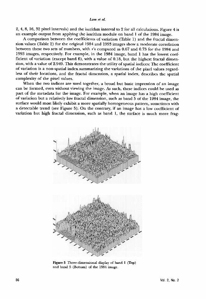
When the two indices are used together, a broad but basic impression of an imagecan be formed, even without viewing the image. As such, these indices could be used aspart of the metadata for the image. For example, when an image has a high coefficientof variation but a relatively low fractal dimension, such as band 5 of the 1984 image, thesurface would most likely exhibit a more spatially homogeneous pattern, sometimes witha detectable trend (see Figure 5). On the contrary, if an image has a low coefficient ofvariation but high fractal dimension, such as band 1, the surface is much more frag-

Figure 5 Three-dimensional display of band 1 (Top)and band 5 (Bottom) of the 1984 image.

86 Vol. 2, No.2


mented and spatially varying. In addition to the traditional nonspatial statistics, thisresult confirms the need to utilize spatial indices in visualizing and detecting environ-mental patterns. The fractal indices used here have added information and served as aquick tool in understanding the spatial dimension of the image.

Multiscale and Multi-Temporal Assessments

To characterize the effects of pixel resolution on the computed indices, the aggregationmodule in ICAMS was applied with a 2 x 2 smoothing/averaging filter to aggregate theoriginal images (201 x 201 pixels) into resampled images with 101 x 101 pixels. Theresampled images were then applied to the fractal module using the same isarithmmethod to re-compute their fractal dimensions. The resultant fractal dimension valuesfor the resampled images are listed in Table 2 and displayed in Figure 3. To enhancecomparison, the coefficients of variation of the resampled images were also computed(see Table 1).

In a multi-scale setting, when comparing the spatial, or fractal dimension, withnon-spatial, or coefficient of variation, results show that coefficients of variation and thefractal dimension values generally decrease with decreasing pixel resolution, except inband 6. The correlation coefficients between the coefficient of variation and the fractaldimension also decrease to a value close to 0.44 for both images. Band 6 exhibits adistinct reverse trend, with much higher fractal dimensions resulted in the resampledimages. This can be easily explained because the original sensor resolution of band 6that was about 120 m was artificially resampled to 25 m to conform with the rest of thebands in Landsat- TM images, resulting in a much smoother and less spatially complexsurface. The 2 x 2 filter applied to this band increased the pixel resolution to 50 x 50 mand in effect reduced the smoothness, thereby resulting in a higher fractal dimension.This aspect of spatial information is not reflected by the coefficient of variation. Ourfindings further suggest the need for more effective spatial indices in characterizingremote sensing images.

Although the following was not tested here, if band 6 is further aggregated, thefractal dimension will continue to increase until the resolution reaches to 120 m, andthereafter, it may increase or decrease. The resolution at which the fractal dimensionyields the highest value can be considered as the scale of action, the "characteristic"scale, or the optimal scale for analysis (Woodcock and Strahler, 1987). The use of fractaldimension in characterizing scale has been suggested earlier (Lam and Quattrochi,1992). With ICAMS, it is easier to perform such analysis for a variety of images.

In terms of spectral band (see Figure 3), the results from all four images, originaland resampled images of the two dates, seem to indicate three groups of spectral bandsbased on their similarity in fractal dimension values. Group A contains bands 1, 2, and 3and has the highest dimensions, whereas group B contains bands 4 and 5 and has lowerdimensions. Group C is band 7, which has a dimension value lying between groups Aand B. As expected, fractal dimension values of the thermal band (band 6) are signifi-cantly lower, because of the smoother surfaces created from resampling from a coarsersensor resolution to a finer resolution. This suggests that the fractal dimension valuescomputed for the spectral bands can be used as a potential guide to select certain bandsfor further analysis. In this case, a band from each of the three groups could be picked,instead of using all six bands, to reduce the complexity and time of analysis normallyrequired for examining all bands. We expect that this kind of application will become


Lam et aT.

more significant and widespread when hyperspectral images such as AVIRIS (AirborneVisible InfraRed Imaging Spectrometer), which has 224 spectral bands, become available.

When the two images from two different dates are compared, Table 2 and thecorresponding Figure 3 show that the 1993 image in general yields lower fractal dimen-sions. Because very little change occurred in Lake Charles during the 9-year period,differences in dimension values may be because of the smaller ranges of spectral reflec-tance and lower maximum values for all bands, except band 6 (see Table 1), rather thanchanges in land cover between the two dates. It is possible that normalization of the twoimages may reduce the differences. It is not known whether the smaller spectral rangesand lower maximum values were caused by a general deterioration of the sensor throughtime or a phenomenon specific to this particular TM scene. Although the computedfractal dimension values have adequately reflected the changes in spectral reflectancevalues, our initial multi-temporal analysis has pointed to the main difficulty in land-coverchange detection, which is to distinguish real land-cover changes from spurious changesdue to ~ctors such as atmosphere, sensor, and sun angle. With ICAMS available, how-ever, mqre images from different regions with similar time periods could be examined,or different techniques, such as band ratio images, could be applied to analyze furtherhow the information on changes in index values can be used effectively in assessing thetrue conditions of environment.

This example has pointed to the need for two analyses in the near future. First, asnoted earlier, accurate comparison of multi-date images requires more elaborate atmo-spheric calibration and/or normalization of the images (jensen, 1996). Although theimpact of not normalizing the images may be minimized because ratios (NDVI), insteadof absolute numbers are used, in the future it would be useful to document the effectsof the various algorithms on calibrated/uncalibrated or normalized/un normalized imag-ery. Second, the fractal module in ICAMS mainly focuses on the computation of globalindices for the entire study area. Local fractal measures, which may reflect changes inlocal areas more effectively, should be further explored and implemented (De long andBurrough, 1995; Mallat, 1989).

Delineation of Boundaries

To demonstrate the utility of lCAMS in delineating major boundaries, we applied theland/water and vegetated/non-vegetated boundary delineation modules to the two images.There are different methods to determine these boundaries, each with its own advan-tages and disadvantages (Cherukuri, 1994). We implemented the NDVI method to delin-eate these boundaries because of its reasonable accuracy, simplicity, and flexibility inallowing the user to visualize and modify the results interactively.

In delineating the boundaries, the NDVI ratio must first be computed. NDVI is aratio between the red and infrared bands. For Landsat- TM images, NDVI is derived from

using:

NDVI = (band 4 -band 3) / (band 4 + band 3).

In general, clouds, snow, water, moist soil, and bright non-vegetated surfaces have NDVIvalues less than zero, rock and dry bare soils have values close to zero, and positive NDVIvalues generally indicate vegetated areas. For example, NDVI values for the contermi-nous United States computed from the 1990 NOAA-AVHRR (Advanced Very High Res-olution Radiometer) images have a range of 0.5 to 0.66 for vegetation (Lillesand andKiefer, 1994). To assist the user in determining the boundaries, we set -0.1 as the default

88 Vol. 2, No.2


threshold value to delineate land and water. Pixels with a value smaller than and equalto -0.1 are classified as water, whereas pixels with a value greater than -0.1 are classifiedas land. Similarly, a value of 0.25 was used as the default threshold value to delineatevegetated and non-vegetated boundaries. As mentioned earlier, these threshold valuescan be easily modified so that changes in boundarjies due to threshold value changes canbe visualized and evaluated. Furthermore, the output can be integrated with other datalayers for further analysis.

Figure 6 shows the land/water boundaries at the two time periods using the defaultthreshold values. Lake Charles, in the upper left corner, is clearly identified as water.The 1984 image generally has more tiny pockets of water pixels than that of the 1993image, which could indicate misclassification. However, by changing the threshold valuefrom the default of -0.1 to a value of -0.2, fewer water pixels were defined. In fact, theredefined boundaries on the 1984 image now resemble closely the land/water bound-aries derived from using the default value on the 1993 image. Detailed research on thevariability of NDVI as well as the accuracy of tht default threshold values in differenttypes of the images is out of the scope of the pre~ent article. The main point, however,is that ICAMS can be used effectively to explore further these various issues.

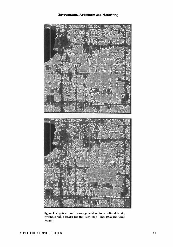
Figure 7 compares the vegetated/non-vegetated boundaries defined by using thesame threshold value (0.25) for the two dates. The 1984 image shows slightly morevegetated areas. The roads and buildings at the southeast corner of the image, whichwere not in the 1984 image, were correctly identified as vegetated areas in 1984 andnonvegetated areas in 1993.

CONCLUSIONS

UsJng two images for Lake Charles, Louisiana, we have demonstrated how ICAMS can beapplied to characterizing temporal differences ilil remote sensing images for environ-mcntal assessment and measurement. We have demonstrated the need for spatial indi-ces, such as fractal dimension, in revealing the spatial characteristics of the images. Usingfractal dimension with the traditional non-spatial statistics, such as coefficient of varia-tion, a basic impression of the image can be foI'med even without viewing the image.These simple indices could serve as part of the metadata of the image that could then beused as a guide to search an image for rapid change detection and monitoring. This typeof library application will have tremendous potemtial when voluminous image data areavailable during the NASA-EOS era. Moreover, fractal dimension values of individualbands could be utilized as a guide for selecting illdividual or combinatiolls of ballds foraIl~ysis. Such applicatioll will be especially useful to the analysis of hyperspectral images.

Through the multi-scale allalysis, we have shown that except for balld 6, fractaldimension values generally decrease with decreasing pixel resolution. The reverse trendshown ill balld 6 further illdicates that fractal illdices could be used, together with otherscale methods, to identify the "characteristic" or optimal scale of analysis. Scale allalysisthrough ICAMS, therefore, call provide a quick assessment of the scale effects 011 thederived illdices alld boulldaries, thus contributing to more accurate enviroIlmeIltal assess-m~nt alld monitoring, and eventually to the deve1.opmellt of more sellsible ellvironmen-tal or lalld-use policies for a regioll.

The developmeIlt of ICAMS is all evolving process, mealling that COIltiIlUOUS improve-mtjIlt to the software will have to be made. Issues such as the reliability of the methodsaIl~ the usefumess of the illdices will have to be further examined. Furthermore, as


Figure 6 Land/water boundaries using athreshold value of -0.1 for the 1984 and 1993images (top and middle) and a thresholdvalue of -0.2 for the 1984 image (bottom).

90 Vol. 2, No.2


Figure 7 Vegetated and non-vegetated regions defined by thethreshold value (0.25) for the 1984 (top) and 1993 (bottom)images.


Lam et at.

hardware and software platforms, as well as data needs and data requirements change,ICAMS will have to be modified. So it can be accessed through the Internet, futureimprovements of ICAMS will include the development of the software on a stand-aloneplatform using computer languages such as JAVA. By making this software available to awider community, we hope that improvement can be made in methods, tools, andinnovative applications. Through application by a diverse user group, ICAMS can evolvefrom the exploratory to the operational stage as a technique for environmental assess-ment and policy development.

REFEREN CES

Burrough, P.A. (1993). Fractals and Geostatistical Methods in Landscape Studies. In Lam, N.S.-N.,and De Cola, L. (eds). Fractal5 in Geography, Englewood C:liffs, NJ: Prentice Hall, pp. 87-121.

Cherukuri, R. (1994). Evaluation of Methods for the Delineation lif Land/"'ater Interface Conditions UsingAVHRR Imagery. M.S. thesis, Department of Geography and Ant.hropology, Louisiana StateUniversity.

Coppin, P.R. and Bauer, M.E. (1994). Processing of Multitemporal Landsat TM Imagery to Opti-mize Extraction of Forest Cover Change Features. IEEE Transactions on Geoscience and RemoteSensing 32 (4), 918-927.

Davis, F.W., Quattrochi, D.A., Ridd, M.K., Lam, N.S.-N, Walsh, SJ., Michaelson, J.C., Franklin, J.,Stow, D.A., Johannsen, CJ., and Johnston, C.A. (1991). Environmental Analysis Using Inte-grated GIS and Remotely Sensed Data: Some Research Needs and Priorities. PhotogrammetricEngineering and Remote Sensing 57,689-697.

De Cola, L. (1989). Fractal Analysis of a Classified Landsat Scene. Photogrammetric Engineering andRemote Sensing 55, 601-610.

Dejong, S.M., and Burrough, P.A. (1995). A Fractal Approach to the Classification of Mediterra-nean Vegetation Types in Remotely Sensed Images. Phot06JTammetric Engineering and Remote Sens-ing 61 (8), 1041-1053.

Falconer, K. (1990). Fractal Geometry. New York, NY: Wiley.Goodchild, M.F. (1986). Spatial Autocorrelation [CATMOG (Concepts and Techniques in Modem

Geography) 47]. Norwich, England: Geo Books.Goodchild, M.F., and Mark, D.M. (1987). The Fractal Nature of Geographic Phenomena. Annal5 of

the Association of American GeograPhers 77 (2), 265-278.Goodchild, M.F., Parks, B.O., and Steyaert, L.T. (1993). Envi1vnmental ,Wodeling with GIS. New York:

Oxford University Press.Jaggi, S.D., Quattrochi, D.A., and Lam, N.S.-N. (1993). Implementation and Operation of Three

Fractal Measurement Algorithms for Analysis of Remote Sensing Data. Computers and Geosciences19(6),745-767.

Jensen,J.R (1996). Introductory Digital Image Processing: A Remote Sensing Perspective. Saddle River, NJ:Prentice-Hall.

Justice, C.O., Bailey, G.B., Maiden, M.E., Rasool, S.I., Strebel, D.E., and Tarpley,J.D. (1995). RecentData and Information System Initiatives for Remotely Sensed Mea.~urements of the Land Sur-face. Remote Sensing of Environment 51 (1), 235-244.

Kineman, JJ. (1993). What is a Scientific Database? Design Considerations for Global Character-ization in the NOAA-EPA Global Ecosystems Database Project. In Goodchild, M.F., Parks, B.O.,and Steyaert, L.T. (eds). Environmental Modeling with GIS. New York: Oxford University Press,pp. 372-378.

KIinkenberg, B. (1994). A Review of Methods Used to Determine the Fractal Dimension of LinearFeatures. Mathematical Geology 26, 23-33.

KIinkenberg, B., and Goodchild, M.F. (1992). The Fractal Properties of Topography: A Comparisonof Methods. Earth Surface Processes and Landforms 17, 217-234.

Lam, N.S.-N. (1990). Description and Measurement of Landsat TM Image U.~ing Fractals. Photo-gram metric Engineering and Remote Sensing 56, 187-195.

92 Vol. 2, No.2

Environmental Assessment and Monitoling

Lam, N.S.-N., and Quattrochi, D.A. (1992). On the Issue of Scale, Resolution, and Fractal Analysisin the Mapping Sciences. The Professional GeograPher 44 (1), 88-98.

Lam, N.S.-N., and De Cola, L. (eds.) (1993). Fractals in {;eograPhy. Englewood Cliffs, NJ: PrenticeHall.

Lam, N.S.-N., Fan, M., and Liu, K.B. (1996). Spatial-Temporal Spread of the AIDS Epidemic: ACorrelogram Analysis of Four Regions of the United States. GeograPhical Analysis 28 (2),93-107.

Lillesand, T.M., and Kiefer, R.W. (1994). Remote Sensing and Image InJerpretation (3rd ed.). New York:Wiley.

Lobitz, B. (1994). Correlations of Vegetation with Surface Ternperature in Three Louisiana Cities. M.L.A.thesis, School of Landscape Architecture, Louisiana State University.

Lovejoy, S., and Schertzer, D. (1988). Extreme Variability, Scaling and Fractals in Remote Sensing:Analysis and Simulation. In Muller, J.P. (ed). Digital Image Processing in Remote Sensing. Philadel-phia: Taylor & Francis, pp. 177-212.

Lovejoy, S., and Schertzer, D. (1990). Multifractals, Universality C;lasses and Satellite and RadarMeasurements of Cloud and Rain Fields. Journal of Geophysicallwsearch 95 (D3), 2021-2034.

Mallat, S.G. (1989). A Theory for Multiresolution Signal Decomposition: The Wavelet Represen-tation. IEEE Transactions on Pattern Analysis and Machine Intelligence PAM-II (7), 674-693.

Mark, D.M., and Aronson, P.B. (1984). Scale-Dependent Fractal Dimensions of Topographic Sur-faces: An Empirical Investigation, with Applications in Geomorphology and Computer Map-ping. Mathematical Geology 11, 671-684.

Markham, B.L., and Barker, J.L. (1986). Landsat MSS and TM Post-Calibration Dynamic Ranges,Exoatmospheric Reflectances and At-Satellite Temperatures. EOSAT Landsat Technical Notes 1,3-8.

Mandelbrot, B. (1977). Fractals: Form, Chance and Dimension. New York: W.H. Freeman and Co.Mandelbrot, B. (1983). The Fractal Geometry of Nature. New York: W.H. Freeman and Co.Olsen, E.R., Ramsey, R.D., and Winn, D.S. (1993). A Modified Fractal Dimension as a Measpre of

Landscape Diversity. Photogrammetric Engineering and Remote Sensing 59 (10), 1517-1520.Quattrochi, Q.A., and Goodchild, M.F. (1997). Scale in Rerrtote Sensing and GIS. Boca Raton, FL: CRC

Lewis Publishers.Quattrochi, Q.A., Lam, N.S.-N., Qiu, H.L., and Zhao, W. (1997). Image Characterization and

Modeling System (ICAMS): A Geographic Information System for the Characterization andModeling of Multi-Scale Remote Sensing Data. In Quattrochi, D.A., and Goodchild, M.F. (eds).Scale in Remote Sensing and GIS. Boca Raton, FL: CRC Lewis Publishers, pp. 295-307.

Running, S.W., Justice, C.O., Salomonson, V., et al. (1994). Terrestrial Remote Sensing and Algo-rithms Planned for EOS/MODIS. International Journal of Remote Sensing 15 (17), 3587-3620.

Steyaert, L. T. (1993). A Perspective on the State of Environmental Simulation Modeling. In Good-child, M.F., Parks, B.O., and Steyaert, L.T. (eds): Environmental Modeling with GIS. New York:Oxford University Press, pp. 16-30.

Townshend,J.R.G., and Justice, c.o. (1988). Selecting the Spatial Resolution of Satellite SensorsRequired for Global Monitoring of Land Transformations. International Journal of Remote Sensing9,187-236.

Turner, M.G., Dale, V.H., and Gardner, R.H. (1989a). Predicting across Scales: Theory Develop-ment and Testing. Landscape Ecology 3 (3/4), 245-252.

Turner, M.G., O'Neill, R.V., Gardner, R.H., and Milne, B.T. (1989b). Effects of Changing SpatialScale on the Analysis of Landscape Pattern. Landscape Ecology 3(3/4), 153-162.

Woodcock, C.E., and Strahler, A.H. (1987). The Factor of Scale in Remote Sensing. Remote Sensingof Environment 21,311-332.


nina siu-ngan lam nasa - louisiana state · pdf filenina siu-ngan lam department of geography...

Documents