nimble user manualr-nimble.org/manuals/nimbleusermanual.pdf · nimble user manual nimble...
TRANSCRIPT

NIMBLE User Manual
NIMBLE Development Team
Version 0.6-11
http://R-nimble.orghttps://github.com/nimble-dev/nimble-docs

Contents
I Introduction 6
1 Welcome to NIMBLE 71.1 What does NIMBLE do? . . . . . . . . . . . . . . . . . . . . . . . . . . . . . 71.2 How to use this manual . . . . . . . . . . . . . . . . . . . . . . . . . . . . . . 8
2 Lightning introduction 92.1 A brief example . . . . . . . . . . . . . . . . . . . . . . . . . . . . . . . . . . 92.2 Creating a model . . . . . . . . . . . . . . . . . . . . . . . . . . . . . . . . . 92.3 Compiling the model . . . . . . . . . . . . . . . . . . . . . . . . . . . . . . . 142.4 One-line invocation of MCMC . . . . . . . . . . . . . . . . . . . . . . . . . . 142.5 Creating, compiling and running a basic MCMC configuration . . . . . . . . 152.6 Customizing the MCMC . . . . . . . . . . . . . . . . . . . . . . . . . . . . . 172.7 Running MCEM . . . . . . . . . . . . . . . . . . . . . . . . . . . . . . . . . 182.8 Creating your own functions . . . . . . . . . . . . . . . . . . . . . . . . . . . 20
3 More introduction 233.1 NIMBLE adopts and extends the BUGS language for specifying models . . . 233.2 nimbleFunctions for writing algorithms . . . . . . . . . . . . . . . . . . . . . 243.3 The NIMBLE algorithm library . . . . . . . . . . . . . . . . . . . . . . . . . 25
4 Installing NIMBLE 264.1 Requirements to run NIMBLE . . . . . . . . . . . . . . . . . . . . . . . . . . 264.2 Installing a C++ compiler for NIMBLE to use . . . . . . . . . . . . . . . . . 26
4.2.1 OS X . . . . . . . . . . . . . . . . . . . . . . . . . . . . . . . . . . . . 274.2.2 Linux . . . . . . . . . . . . . . . . . . . . . . . . . . . . . . . . . . . 274.2.3 Windows . . . . . . . . . . . . . . . . . . . . . . . . . . . . . . . . . . 27
4.3 Installing the NIMBLE package . . . . . . . . . . . . . . . . . . . . . . . . . 274.3.1 Problems with installation . . . . . . . . . . . . . . . . . . . . . . . . 28
4.4 Customizing your installation . . . . . . . . . . . . . . . . . . . . . . . . . . 284.4.1 Using your own copy of Eigen . . . . . . . . . . . . . . . . . . . . . . 284.4.2 Using libnimble . . . . . . . . . . . . . . . . . . . . . . . . . . . . . . 284.4.3 BLAS and LAPACK . . . . . . . . . . . . . . . . . . . . . . . . . . . 294.4.4 Customizing compilation of the NIMBLE-generated C++ . . . . . . . 29
1

CONTENTS 2
II Models in NIMBLE 30
5 Writing models in NIMBLE’s dialect of BUGS 315.1 Comparison to BUGS dialects supported by WinBUGS, OpenBUGS and JAGS 31
5.1.1 Supported features of BUGS and JAGS . . . . . . . . . . . . . . . . . 315.1.2 NIMBLE’s Extensions to BUGS and JAGS . . . . . . . . . . . . . . . 315.1.3 Not-yet-supported features of BUGS and JAGS . . . . . . . . . . . . 32
5.2 Writing models . . . . . . . . . . . . . . . . . . . . . . . . . . . . . . . . . . 335.2.1 Declaring stochastic and deterministic nodes . . . . . . . . . . . . . . 335.2.2 More kinds of BUGS declarations . . . . . . . . . . . . . . . . . . . . 365.2.3 Vectorized versus scalar declarations . . . . . . . . . . . . . . . . . . 375.2.4 Available distributions . . . . . . . . . . . . . . . . . . . . . . . . . . 385.2.5 Available BUGS language functions . . . . . . . . . . . . . . . . . . . 435.2.6 Available link functions . . . . . . . . . . . . . . . . . . . . . . . . . . 455.2.7 Truncation, censoring, and constraints . . . . . . . . . . . . . . . . . 46
6 Building and using models 496.1 Creating model objects . . . . . . . . . . . . . . . . . . . . . . . . . . . . . . 49
6.1.1 Using nimbleModel to create a model . . . . . . . . . . . . . . . . . . 496.1.2 Creating a model from standard BUGS and JAGS input files . . . . . 546.1.3 Making multiple instances from the same model definition . . . . . . 54
6.2 NIMBLE models are objects you can query and manipulate . . . . . . . . . 556.2.1 What are variables and nodes? . . . . . . . . . . . . . . . . . . . . . 556.2.2 Determining the nodes and variables in a model . . . . . . . . . . . . 566.2.3 Accessing nodes . . . . . . . . . . . . . . . . . . . . . . . . . . . . . . 576.2.4 How nodes are named . . . . . . . . . . . . . . . . . . . . . . . . . . 586.2.5 Why use node names? . . . . . . . . . . . . . . . . . . . . . . . . . . 596.2.6 Checking if a node holds data . . . . . . . . . . . . . . . . . . . . . . 59
III Algorithms in NIMBLE 60
7 MCMC 617.1 One-line invocation of MCMC: nimbleMCMC . . . . . . . . . . . . . . . . . . 627.2 The MCMC configuration . . . . . . . . . . . . . . . . . . . . . . . . . . . . 63
7.2.1 Default MCMC configuration . . . . . . . . . . . . . . . . . . . . . . 647.2.2 Customizing the MCMC configuration . . . . . . . . . . . . . . . . . 65
7.3 Building and compiling the MCMC . . . . . . . . . . . . . . . . . . . . . . . 717.4 User-friendly execution of MCMC algorithms: runMCMC . . . . . . . . . . . . 727.5 Running the MCMC . . . . . . . . . . . . . . . . . . . . . . . . . . . . . . . 74
7.5.1 Measuring sampler computation times: getTimes . . . . . . . . . . . 747.6 Extracting MCMC samples . . . . . . . . . . . . . . . . . . . . . . . . . . . 747.7 Calculating WAIC . . . . . . . . . . . . . . . . . . . . . . . . . . . . . . . . 757.8 k-fold cross-validation . . . . . . . . . . . . . . . . . . . . . . . . . . . . . . . 757.9 Samplers provided with NIMBLE . . . . . . . . . . . . . . . . . . . . . . . . 75

CONTENTS 3
7.9.1 Conjugate (‘Gibbs’) samplers . . . . . . . . . . . . . . . . . . . . . . 767.9.2 Customized log-likelihood evaluations: RW llFunction sampler . . . . 777.9.3 Particle MCMC PMCMC sampler . . . . . . . . . . . . . . . . . . . . . 78
7.10 Detailed MCMC example: litters . . . . . . . . . . . . . . . . . . . . . . . 787.11 Comparing different MCMCs with MCMCsuite and compareMCMCs . . . . . . 82
7.11.1 MCMC Suite example: litters . . . . . . . . . . . . . . . . . . . . . 827.11.2 MCMC Suite outputs . . . . . . . . . . . . . . . . . . . . . . . . . . . 837.11.3 Customizing MCMC Suite . . . . . . . . . . . . . . . . . . . . . . . . 84
8 Sequential Monte Carlo and MCEM 878.1 Particle Filters / Sequential Monte Carlo . . . . . . . . . . . . . . . . . . . . 87
8.1.1 Filtering Algorithms . . . . . . . . . . . . . . . . . . . . . . . . . . . 878.1.2 Particle MCMC (PMCMC) . . . . . . . . . . . . . . . . . . . . . . . 90
8.2 Monte Carlo Expectation Maximization (MCEM) . . . . . . . . . . . . . . . 928.2.1 Estimating the Asymptotic Covariance From MCEM . . . . . . . . . 94
9 Spatial models 959.1 Intrinsic Gaussian CAR model: dcar normal . . . . . . . . . . . . . . . . . . 95
9.1.1 Specification and density . . . . . . . . . . . . . . . . . . . . . . . . . 959.1.2 Example . . . . . . . . . . . . . . . . . . . . . . . . . . . . . . . . . . 97
9.2 Proper Gaussian CAR model: dcar proper . . . . . . . . . . . . . . . . . . 989.2.1 Specification and density . . . . . . . . . . . . . . . . . . . . . . . . . 989.2.2 Example . . . . . . . . . . . . . . . . . . . . . . . . . . . . . . . . . . 100
9.3 MCMC Sampling of CAR models . . . . . . . . . . . . . . . . . . . . . . . . 1019.3.1 Initial values . . . . . . . . . . . . . . . . . . . . . . . . . . . . . . . 1019.3.2 Zero-neighbor regions . . . . . . . . . . . . . . . . . . . . . . . . . . . 1029.3.3 Zero-mean constraint . . . . . . . . . . . . . . . . . . . . . . . . . . . 102
10 Bayesian nonparametric models 10310.1 Bayesian nonparametric mixture models . . . . . . . . . . . . . . . . . . . . 10310.2 Chinese Restaurant Process model . . . . . . . . . . . . . . . . . . . . . . . 104
10.2.1 Specification and density . . . . . . . . . . . . . . . . . . . . . . . . . 10410.2.2 Example . . . . . . . . . . . . . . . . . . . . . . . . . . . . . . . . . . 105
10.3 Stick-breaking model . . . . . . . . . . . . . . . . . . . . . . . . . . . . . . . 10610.3.1 Specification and function . . . . . . . . . . . . . . . . . . . . . . . . 10610.3.2 Example . . . . . . . . . . . . . . . . . . . . . . . . . . . . . . . . . . 107
10.4 MCMC sampling of BNP models . . . . . . . . . . . . . . . . . . . . . . . . 10810.4.1 Sampling CRP models . . . . . . . . . . . . . . . . . . . . . . . . . . 10810.4.2 Sampling stick-breaking models . . . . . . . . . . . . . . . . . . . . . 109
IV Programming with NIMBLE 111
11 Writing simple nimbleFunctions 11311.1 Introduction to simple nimbleFunctions . . . . . . . . . . . . . . . . . . . . . 113

CONTENTS 4
11.2 R functions (or variants) implemented in NIMBLE . . . . . . . . . . . . . . 11411.2.1 Finding help for NIMBLE’s versions of R functions . . . . . . . . . . 11411.2.2 Basic operations . . . . . . . . . . . . . . . . . . . . . . . . . . . . . 11511.2.3 Math and linear algebra . . . . . . . . . . . . . . . . . . . . . . . . . 11711.2.4 Distribution functions . . . . . . . . . . . . . . . . . . . . . . . . . . 11911.2.5 Flow control: if-then-else, for, while, and stop . . . . . . . . . . 12011.2.6 print and cat . . . . . . . . . . . . . . . . . . . . . . . . . . . . . . 12011.2.7 Checking for user interrupts: checkInterrupt . . . . . . . . . . . . . 12111.2.8 Optimization: optim and nimOptim . . . . . . . . . . . . . . . . . . . 12111.2.9 “nim” synonyms for some functions . . . . . . . . . . . . . . . . . . . 121
11.3 How NIMBLE handles types of variables . . . . . . . . . . . . . . . . . . . . 12211.3.1 nimbleList data structures . . . . . . . . . . . . . . . . . . . . . . . 12211.3.2 How numeric types work . . . . . . . . . . . . . . . . . . . . . . . . . 122
11.4 Declaring argument and return types . . . . . . . . . . . . . . . . . . . . . . 12511.5 Compiled nimbleFunctions pass arguments by reference . . . . . . . . . . . . 12611.6 Calling external compiled code . . . . . . . . . . . . . . . . . . . . . . . . . . 12611.7 Calling uncompiled R functions from compiled nimbleFunctions . . . . . . 126
12 Creating user-defined BUGS distributions and functions 12812.1 User-defined functions . . . . . . . . . . . . . . . . . . . . . . . . . . . . . . 12812.2 User-defined distributions . . . . . . . . . . . . . . . . . . . . . . . . . . . . 129
12.2.1 Using registerDistributions for alternative parameterizations andproviding other information . . . . . . . . . . . . . . . . . . . . . . . 132
13 Working with NIMBLE models 13413.1 The variables and nodes in a NIMBLE model . . . . . . . . . . . . . . . . . 134
13.1.1 Determining the nodes in a model . . . . . . . . . . . . . . . . . . . . 13413.1.2 Understanding lifted nodes . . . . . . . . . . . . . . . . . . . . . . . . 13613.1.3 Determining dependencies in a model . . . . . . . . . . . . . . . . . . 137
13.2 Accessing information about nodes and variables . . . . . . . . . . . . . . . . 13813.2.1 Getting distributional information about a node . . . . . . . . . . . . 13813.2.2 Getting information about a distribution . . . . . . . . . . . . . . . . 13913.2.3 Getting distribution parameter values for a node . . . . . . . . . . . . 13913.2.4 Getting distribution bounds for a node . . . . . . . . . . . . . . . . . 140
13.3 Carrying out model calculations . . . . . . . . . . . . . . . . . . . . . . . . . 14113.3.1 Core model operations: calculation and simulation . . . . . . . . . . . 14113.3.2 Pre-defined nimbleFunctions for operating on model nodes: simNodes,
calcNodes, and getLogProbNodes . . . . . . . . . . . . . . . . . . . 14313.3.3 Accessing log probabilities via logProb variables . . . . . . . . . . . . 145
14 Data structures in NIMBLE 14714.1 The modelValues data structure . . . . . . . . . . . . . . . . . . . . . . . . . 147
14.1.1 Creating modelValues objects . . . . . . . . . . . . . . . . . . . . . . 14714.1.2 Accessing contents of modelValues . . . . . . . . . . . . . . . . . . . 149
14.2 The nimbleList data structure . . . . . . . . . . . . . . . . . . . . . . . . . . 153

CONTENTS 5
14.2.1 Using eigen and svd in nimbleFunctions . . . . . . . . . . . . . . . . 155
15 Writing nimbleFunctions to interact with models 15815.1 Overview . . . . . . . . . . . . . . . . . . . . . . . . . . . . . . . . . . . . . . 15815.2 Using and compiling nimbleFunctions . . . . . . . . . . . . . . . . . . . . . . 16015.3 Writing setup code . . . . . . . . . . . . . . . . . . . . . . . . . . . . . . . . 161
15.3.1 Useful tools for setup functions . . . . . . . . . . . . . . . . . . . . . 16115.3.2 Accessing and modifying numeric values from setup . . . . . . . . . . 16115.3.3 Determining numeric types in nimbleFunctions . . . . . . . . . . . . . 16215.3.4 Control of setup outputs . . . . . . . . . . . . . . . . . . . . . . . . . 162
15.4 Writing run code . . . . . . . . . . . . . . . . . . . . . . . . . . . . . . . . . 16215.4.1 Driving models: calculate, calculateDiff, simulate, getLogProb 16215.4.2 Getting and setting variable and node values . . . . . . . . . . . . . . 16315.4.3 Getting parameter values and node bounds . . . . . . . . . . . . . . . 16515.4.4 Using modelValues objects . . . . . . . . . . . . . . . . . . . . . . . . 16515.4.5 Using model variables and modelValues in expressions . . . . . . . . . 16915.4.6 Including other methods in a nimbleFunction . . . . . . . . . . . . . 17015.4.7 Using other nimbleFunctions . . . . . . . . . . . . . . . . . . . . . . . 17115.4.8 Virtual nimbleFunctions and nimbleFunctionLists . . . . . . . . . . . 17215.4.9 Character objects . . . . . . . . . . . . . . . . . . . . . . . . . . . . . 17415.4.10 User-defined data structures . . . . . . . . . . . . . . . . . . . . . . . 174
15.5 Example: writing user-defined samplers to extend NIMBLE’s MCMC engine 17615.6 Copying nimbleFunctions (and NIMBLE models) . . . . . . . . . . . . . . . 17815.7 Debugging nimbleFunctions . . . . . . . . . . . . . . . . . . . . . . . . . . . 17815.8 Timing nimbleFunctions with run.time . . . . . . . . . . . . . . . . . . . . . 17815.9 Reducing memory usage . . . . . . . . . . . . . . . . . . . . . . . . . . . . . 179

Part I
Introduction
6

Chapter 1
Welcome to NIMBLE
NIMBLE is a system for building and sharing analysis methods for statistical models from R,especially for hierarchical models and computationally-intensive methods. While NIMBLEis embedded in R, it goes beyond R by supporting separate programming of models andalgorithms along with compilation for fast execution.
As of version 0.6-11, NIMBLE has been around for a while and is reasonably stable, but wehave a lot of plans to expand and improve it. The algorithm library provides MCMC with alot of user control and ability to write new samplers easily. Other algorithms include particlefiltering (sequential Monte Carlo) and Monte Carlo Expectation Maximization (MCEM).
But NIMBLE is about much more than providing an algorithm library. It provides alanguage for writing model-generic algorithms. We hope you will program in NIMBLE andmake an R package providing your method. Of course, NIMBLE is open source, so we alsohope you’ll contribute to its development.
Please join the mailing lists (see R-nimble.org/more/issues-and-groups) and help improveNIMBLE by telling us what you want to do with it, what you like, and what could be better.We have a lot of ideas for how to improve it, but we want your help and ideas too. You canalso follow and contribute to developer discussions on the wiki of our GitHub repository.
If you use NIMBLE in your work, please cite us, as this helps justify past and future fund-ing for the development of NIMBLE. For more information, please call citation(’nimble’)in R.
1.1 What does NIMBLE do?
NIMBLE makes it easier to program statistical algorithms that will run efficiently and workon many different models from R.
You can think of NIMBLE as comprising four pieces:
1. A system for writing statistical models flexibly, which is an extension of the BUGSlanguage1.
2. A library of algorithms such as MCMC.
1See Chapter 5 for information about NIMBLE’s version of BUGS.
7

CHAPTER 1. WELCOME TO NIMBLE 8
3. A language, called NIMBLE, embedded within and similar in style to R, for writingalgorithms that operate on models written in BUGS.
4. A compiler that generates C++ for your models and algorithms, compiles that C++,and lets you use it seamlessly from R without knowing anything about C++.
NIMBLE stands for Numerical Inference for statistical Models for Bayesian and Likeli-hood Estimation.
Although NIMBLE was motivated by algorithms for hierarchical statistical models, it’suseful for other goals too. You could use it for simpler models. And since NIMBLE canautomatically compile R-like functions into C++ that use the Eigen library for fast linearalgebra, you can use it to program fast numerical functions without any model involved2
One of the beauties of R is that many of the high-level analysis functions are themselveswritten in R, so it is easy to see their code and modify them. The same is true for NIMBLE:the algorithms are themselves written in the NIMBLE language.
1.2 How to use this manual
We suggest everyone start with the Lightning Introduction in Chapter 2.Then, if you want to jump into using NIMBLE’s algorithms without learning about
NIMBLE’s programming system, go to Part II to learn how to build your model and PartIII to learn how to apply NIMBLE’s built-in algorithms to your model.
If you want to learn about NIMBLE programming (nimbleFunctions), go to Part IV. Thisteaches how to program user-defined function or distributions to use in BUGS code, compileyour R code for faster operations, and write algorithms with NIMBLE. These algorithmscould be specific algorithms for your particular model (such as a user-defined MCMC samplerfor a parameter in your model) or general algorithms you can distribute to others. Infact the algorithms provided as part of NIMBLE and described in Part III are written asnimbleFunctions.
2The packages Rcpp and RcppEigen provide different ways of connecting C++, the Eigen library and R.In those packages you program directly in C++, while in NIMBLE you program in R in a nimbleFunctionand the NIMBLE compiler turns it into C++.

Chapter 2
Lightning introduction
2.1 A brief example
Here we’ll give a simple example of building a model and running some algorithms on themodel, as well as creating our own user-specified algorithm. The goal is to give you a sensefor what one can do in the system. Later sections will provide more detail.
We’ll use the pump model example from BUGS1. We could load the model from thestandard BUGS example file formats (Section 6.1.2), but instead we’ll show how to enter itdirectly in R.
In this “lightning introduction” we will:
1. Create the model for the pump example.2. Compile the model.3. Create a basic MCMC configuration for the pump model.4. Compile and run the MCMC5. Customize the MCMC configuration and compile and run that.6. Create, compile and run a Monte Carlo Expectation Maximization (MCEM) algorithm,
which illustrates some of the flexibility NIMBLE provides to combine R and NIMBLE.7. Write a short nimbleFunction to generate simulations from designated nodes of any
model.
2.2 Creating a model
First we define the model code, its constants, data, and initial values for MCMC.
pumpCode <- nimbleCode({for (i in 1:N){
theta[i] ~ dgamma(alpha,beta)
lambda[i] <- theta[i]*t[i]
x[i] ~ dpois(lambda[i])
1The data set describes failure rates of some pumps.
9
CHAPTER 2. LIGHTNING INTRODUCTION 10
}alpha ~ dexp(1.0)
beta ~ dgamma(0.1,1.0)
})
pumpConsts <- list(N = 10,
t = c(94.3, 15.7, 62.9, 126, 5.24,
31.4, 1.05, 1.05, 2.1, 10.5))
pumpData <- list(x = c(5, 1, 5, 14, 3, 19, 1, 1, 4, 22))
pumpInits <- list(alpha = 1, beta = 1,
theta = rep(0.1, pumpConsts$N))
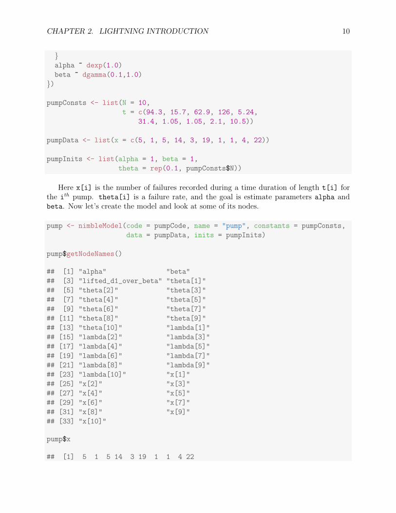
Here x[i] is the number of failures recorded during a time duration of length t[i] forthe ith pump. theta[i] is a failure rate, and the goal is estimate parameters alpha andbeta. Now let’s create the model and look at some of its nodes.
pump <- nimbleModel(code = pumpCode, name = "pump", constants = pumpConsts,
data = pumpData, inits = pumpInits)
pump$getNodeNames()
## [1] "alpha" "beta"
## [3] "lifted_d1_over_beta" "theta[1]"
## [5] "theta[2]" "theta[3]"
## [7] "theta[4]" "theta[5]"
## [9] "theta[6]" "theta[7]"
## [11] "theta[8]" "theta[9]"
## [13] "theta[10]" "lambda[1]"
## [15] "lambda[2]" "lambda[3]"
## [17] "lambda[4]" "lambda[5]"
## [19] "lambda[6]" "lambda[7]"
## [21] "lambda[8]" "lambda[9]"
## [23] "lambda[10]" "x[1]"
## [25] "x[2]" "x[3]"
## [27] "x[4]" "x[5]"
## [29] "x[6]" "x[7]"
## [31] "x[8]" "x[9]"
## [33] "x[10]"
pump$x
## [1] 5 1 5 14 3 19 1 1 4 22

CHAPTER 2. LIGHTNING INTRODUCTION 11
pump$logProb_x
## [1] -2.998011 -1.118924 -1.882686 -2.319466 -4.254550
## [6] -20.739651 -2.358795 -2.358795 -9.630645 -48.447798
pump$alpha
## [1] 1
pump$theta
## [1] 0.1 0.1 0.1 0.1 0.1 0.1 0.1 0.1 0.1 0.1
pump$lambda
## [1] 9.430 1.570 6.290 12.600 0.524 3.140 0.105 0.105
## [9] 0.210 1.050
Notice that in the list of nodes, NIMBLE has introduced a new node, lifted d1 over beta.We call this a “lifted” node. Like R, NIMBLE allows alternative parameterizations, such asthe scale or rate parameterization of the gamma distribution. Choice of parameterizationcan generate a lifted node, as can using a link function or a distribution argument that isan expression. It’s helpful to know why they exist, but you shouldn’t need to worry aboutthem.
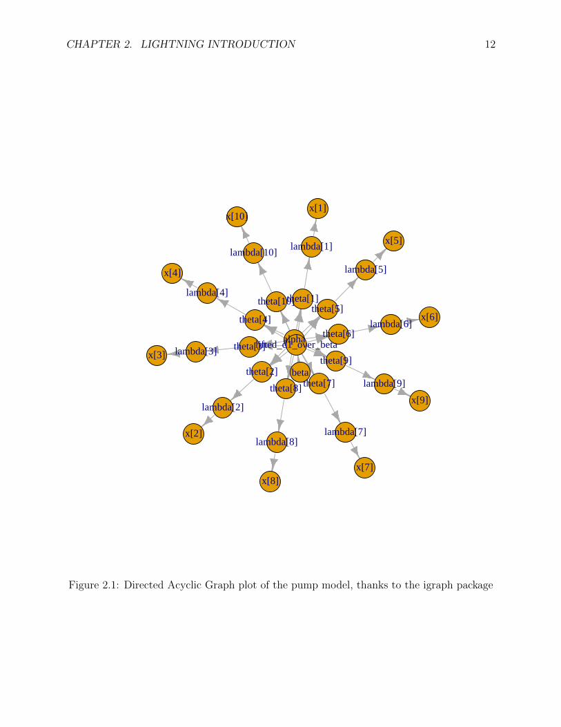
Thanks to the plotting capabilities of the igraph package that NIMBLE uses to representthe directed acyclic graph, we can plot the model (Figure 2.1).
pump$plotGraph()
You are in control of the model. By default, nimbleModel does its best to initialize amodel, but let’s say you want to re-initialize theta. To simulate from the prior for theta
(overwriting the initial values previously in the model) we first need to be sure the parentnodes of all theta[i] nodes are fully initialized, including any non-stochastic nodes suchas lifted nodes. We then use the simulate function to simulate from the distribution fortheta. Finally we use the calculate function to calculate the dependencies of theta,namely lambda and the log probabilities of x to ensure all parts of the model are up to date.First we show how to use the model’s getDependencies method to query information aboutits graph.
## Show all dependencies of alpha and beta terminating in stochastic nodes
pump$getDependencies(c("alpha", "beta"))
## [1] "alpha" "beta"
## [3] "lifted_d1_over_beta" "theta[1]"
## [5] "theta[2]" "theta[3]"
CHAPTER 2. LIGHTNING INTRODUCTION 12
alpha
beta
lifted_d1_over_beta
theta[1]
theta[2]
theta[3]
theta[4]theta[5]
theta[6]
theta[7]theta[8]
theta[9]
theta[10]
lambda[1]
lambda[2]
lambda[3]
lambda[4]
lambda[5]
lambda[6]
lambda[7]lambda[8]
lambda[9]
lambda[10]
x[1]
x[2]
x[3]
x[4]
x[5]
x[6]
x[7]x[8]
x[9]
x[10]
Figure 2.1: Directed Acyclic Graph plot of the pump model, thanks to the igraph package
CHAPTER 2. LIGHTNING INTRODUCTION 13
## [7] "theta[4]" "theta[5]"
## [9] "theta[6]" "theta[7]"
## [11] "theta[8]" "theta[9]"
## [13] "theta[10]"
## Now show only the deterministic dependencies
pump$getDependencies(c("alpha", "beta"), determOnly = TRUE)
## [1] "lifted_d1_over_beta"
## Check that the lifted node was initialized.
pump[["lifted_d1_over_beta"]] ## It was.
## [1] 1
## Now let's simulate new theta values
set.seed(1) ## This makes the simulations here reproducible
pump$simulate("theta")
pump$theta ## the new theta values
## [1] 0.15514136 1.88240160 1.80451250 0.83617765 1.22254365
## [6] 1.15835525 0.99001994 0.30737332 0.09461909 0.15720154
## lambda and logProb_x haven't been re-calculated yet
pump$lambda ## these are the same values as above
## [1] 9.430 1.570 6.290 12.600 0.524 3.140 0.105 0.105
## [9] 0.210 1.050
pump$logProb_x
## [1] -2.998011 -1.118924 -1.882686 -2.319466 -4.254550
## [6] -20.739651 -2.358795 -2.358795 -9.630645 -48.447798
pump$getLogProb("x") ## The sum of logProb_x
## [1] -96.10932
pump$calculate(pump$getDependencies(c("theta")))
## [1] -262.204
pump$lambda ## Now they have.
## [1] 14.6298299 29.5537051 113.5038360 105.3583839 6.4061287
## [6] 36.3723548 1.0395209 0.3227420 0.1987001 1.6506161
pump$logProb_x
## [1] -6.002009 -26.167496 -94.632145 -65.346457 -2.626123
## [6] -7.429868 -1.000761 -1.453644 -9.840589 -39.096527
CHAPTER 2. LIGHTNING INTRODUCTION 14
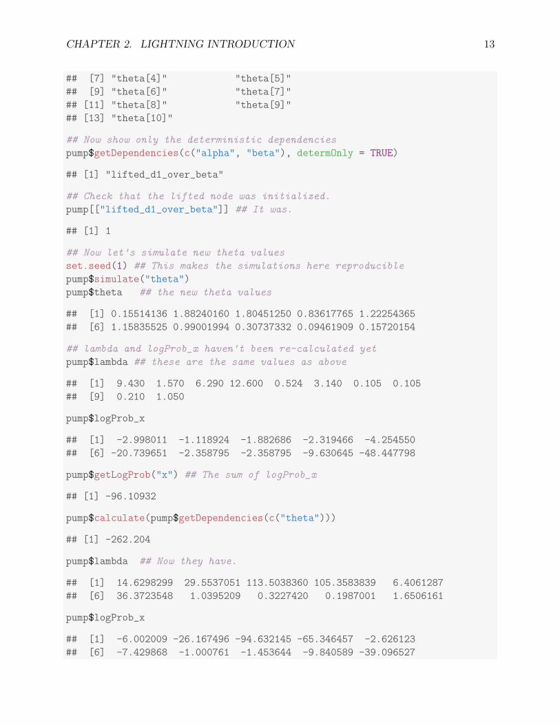
Notice that the first getDependencies call returned dependencies from alpha and beta
down to the next stochastic nodes in the model. The second call requested only deterministicdependencies. The call to pump$simulate("theta") expands "theta" to include all nodesin theta. After simulating into theta, we can see that lambda and the log probabilities ofx still reflect the old values of theta, so we calculate them and then see that they havebeen updated.
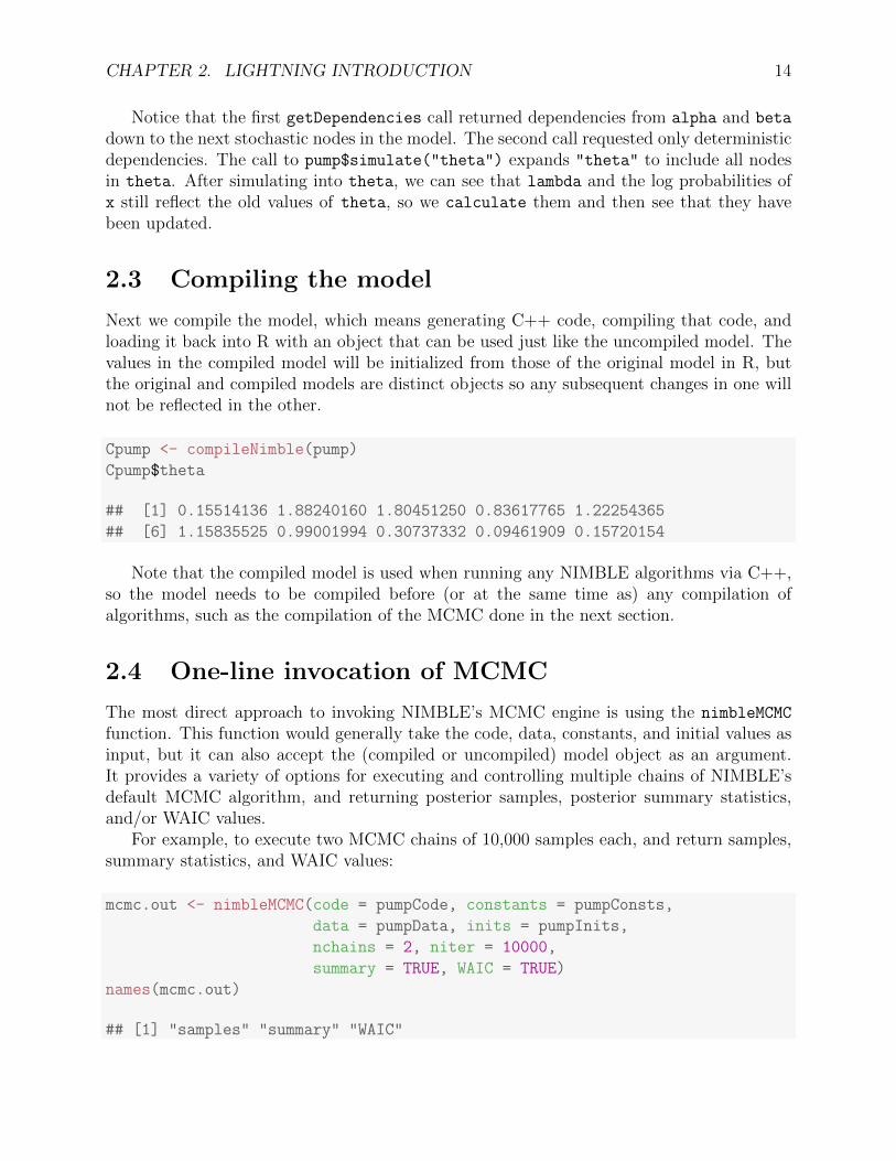
2.3 Compiling the model
Next we compile the model, which means generating C++ code, compiling that code, andloading it back into R with an object that can be used just like the uncompiled model. Thevalues in the compiled model will be initialized from those of the original model in R, butthe original and compiled models are distinct objects so any subsequent changes in one willnot be reflected in the other.
Cpump <- compileNimble(pump)
Cpump$theta
## [1] 0.15514136 1.88240160 1.80451250 0.83617765 1.22254365
## [6] 1.15835525 0.99001994 0.30737332 0.09461909 0.15720154
Note that the compiled model is used when running any NIMBLE algorithms via C++,so the model needs to be compiled before (or at the same time as) any compilation ofalgorithms, such as the compilation of the MCMC done in the next section.
2.4 One-line invocation of MCMC
The most direct approach to invoking NIMBLE’s MCMC engine is using the nimbleMCMC
function. This function would generally take the code, data, constants, and initial values asinput, but it can also accept the (compiled or uncompiled) model object as an argument.It provides a variety of options for executing and controlling multiple chains of NIMBLE’sdefault MCMC algorithm, and returning posterior samples, posterior summary statistics,and/or WAIC values.
For example, to execute two MCMC chains of 10,000 samples each, and return samples,summary statistics, and WAIC values:
mcmc.out <- nimbleMCMC(code = pumpCode, constants = pumpConsts,
data = pumpData, inits = pumpInits,
nchains = 2, niter = 10000,
summary = TRUE, WAIC = TRUE)
names(mcmc.out)
## [1] "samples" "summary" "WAIC"

CHAPTER 2. LIGHTNING INTRODUCTION 15
mcmc.out$summary
## $chain1
## Mean Median St.Dev. 95%CI_low 95%CI_upp
## alpha 0.6980435 0.6583506 0.2703768 0.2878982 1.314046
## beta 0.9286260 0.8215685 0.5496913 0.1836991 2.287270
##
## $chain2
## Mean Median St.Dev. 95%CI_low 95%CI_upp
## alpha 0.6910196 0.6580365 0.2654838 0.2771956 1.285815
## beta 0.9162727 0.8143443 0.5375082 0.1857723 2.270243
##
## $all.chains
## Mean Median St.Dev. 95%CI_low 95%CI_upp
## alpha 0.6945316 0.6580365 0.2679578 0.2832985 1.299932
## beta 0.9224494 0.8182816 0.5436554 0.1854908 2.278544
mcmc.out$waic
## NULL
See Section 7.1 or help(nimbleMCMC) for more details about using nimbleMCMC.
2.5 Creating, compiling and running a basic MCMC
configuration
At this point we have initial values for all of the nodes in the model, and we have both theoriginal and compiled versions of the model. As a first algorithm to try on our model, let’suse NIMBLE’s default MCMC. Note that conjugate relationships are detected for all nodesexcept for alpha, on which the default sampler is a random walk Metropolis sampler.
pumpConf <- configureMCMC(pump, print = TRUE)
## [1] RW sampler: alpha
## [2] conjugate_dgamma_dgamma sampler: beta
## [3] conjugate_dgamma_dpois sampler: theta[1]
## [4] conjugate_dgamma_dpois sampler: theta[2]
## [5] conjugate_dgamma_dpois sampler: theta[3]
## [6] conjugate_dgamma_dpois sampler: theta[4]
## [7] conjugate_dgamma_dpois sampler: theta[5]
## [8] conjugate_dgamma_dpois sampler: theta[6]
## [9] conjugate_dgamma_dpois sampler: theta[7]
## [10] conjugate_dgamma_dpois sampler: theta[8]
## [11] conjugate_dgamma_dpois sampler: theta[9]

CHAPTER 2. LIGHTNING INTRODUCTION 16
## [12] conjugate_dgamma_dpois sampler: theta[10]
pumpConf$addMonitors(c("alpha", "beta", "theta"))
## thin = 1: alpha, beta, theta
pumpMCMC <- buildMCMC(pumpConf)
CpumpMCMC <- compileNimble(pumpMCMC, project = pump)
niter <- 1000
set.seed(1)
CpumpMCMC$run(niter)
## NULL
samples <- as.matrix(CpumpMCMC$mvSamples)
par(mfrow = c(1, 4), mai = c(.6, .4, .1, .2))
plot(samples[ , "alpha"], type = "l", xlab = "iteration",
ylab = expression(alpha))
plot(samples[ , "beta"], type = "l", xlab = "iteration",
ylab = expression(beta))
plot(samples[ , "alpha"], samples[ , "beta"], xlab = expression(alpha),
ylab = expression(beta))
plot(samples[ , "theta[1]"], type = "l", xlab = "iteration",
ylab = expression(theta[1]))
0 400 800
0.5
1.0
1.5
iteration
α
0 400 800
0.0
0.5
1.0
1.5
2.0
2.5
3.0
iteration
β
●●
●
●
●
●
●
●●●
●
●
●
●
●
●●
●
●
●●●●
●
●
●
●
●●
●
●
●
●
●
●
●●
●
●
●
●
●
●
●
●
●
●●
●
●
●
●
●●●●
●●●
●
● ●
●
● ●
●
●
●
●
●
●
●
●
●
●
●
●
●
●
●
●
●
●
●
●
●●
●
●●
●●
●
●
●●
●●
●
●
●
●
●
●
●
●
●●●●
●
●
●
●
●●
●
●
●
●
●●●
●●
●
●
●
●
●
●
●
●
●
●
●
●
●●
●
●●
●
●
●
●
●
●
●●
●
●
●
●●
●●●●●
●
●
●
●
●
●
●
●●
●
●●
●●
●●●
●●
●●
● ●
●
●
●
●
●
●
●●●
●
●
●●
●
●
●
●
●
●
●
●
●
●●●
●
●
●
●●
●●
● ●
●
●●
●
●
●
●●
●
●
●
●
●
●
●
●●●●
●
● ●
●●●●●
●
●●●
●
●
●
●
●
●●
●
●●
●
●●
●●
●
●
●
●
●
●
●
●
●
●
●●
●●
●
●
●
●●●
●
●
●
●
●●
●●
●
●
●●
●●
●●
●
●
●
●
●
●
●
●
●
●
●
●
●
●
●
●●
●
●●●
●
●
●
●
●
●
●●
●
●
●
●●
●
●
●
●
●
●
●
●●
●●
●
●
●
●
●
●
●
●
●
●
●
●
●
●
●
●●●
●
●●
●●
●
●
●
●●
●
●
●
●
●
●●
●●
●
●
●
●●●
●●
●
●
●●
●
●
●
●
●
●
●
●
●
●
●
●
●
●
●
●●
●
●●
●
●
●
●●●
●
●●
●
●
●
●
●●●
●
●
●
●
●●●
●
●●
●
●
●
●
●
●●●
●
●
●●●●●●
●●
●
●●●
●
●●
●
●
●
●
●●
●●
●
●
●●
●
●
●
●
●●
●
●
●●
●
●
●
●
●
●
●●
●
●●
●●●
●●
●
●●
●
●
●●
●
●
●
●
●
●
●
●
●
●
●
●
●●
●
●
●
●●
●
●
●●
●
●
●
●●●
●●
●●●
●●●●
●
●
●●
●
●
●
●
●
●●
●●●
●
●●●●●●
●
●
●
●●
●
●
●●
●●
●
●
●●●
●
●
●
●
●
●
●●
●●●
●●●●
●●
●
●
●
●
●
●●●
●●
●
●
●
●
●
●
●●
●
●
●
●
●●
●
●
●●
●
●
●
●
●
●
●
●
●
●
●
●
●●
●
●●
●
●
●
●
●●●●●●
●
●
●
●
●
●
●
●●
●
●●
●
●●
●
●
●●
●
●
●
●
●
●
●
●●
●●
●●
●
●
●
●
●●
●
●●
●
●
●
●
●
●
●
●
●●●●
●●
●
●
●
●
●●
●●
●●
●●●
●
●●
●
●●
●
●
●
●
●●
●
●
●●
●
●
●
●
●
●
●
●
●
● ●●
●
●
●
●
●
●
●
●
●
●●●
●
●
●●
●
●●
●
●
●●
●
● ●●
●
●●
●
●●
●●
●●
●●
●
●
●
●●
●
●
●●
●●
●
●
●
●
●
●
●●●
●
●
●
●
●●
●
●●●
●
●
●●
●
●
●
●
● ●●●
●
●
●
●
●
●●
●
●
●
●●
●
●
●
●
●
●
●
●●
●
●
●
●
●
●
●●
●
●
●
●
●●
●●
●
●
●
●
●
●
●●
●●●
●
●
●●
●
●●●
●●
●
●
●●
●
●
●●
●●
●●
●●
●
●
●
●
●
●●
●
●
●
●
●
●●●
●
●●●●●
●
●
●●●●
●
●●
●●
●
●
●
●
●
●
●
●
●
●
●●
●●
●●●
●●
●
●
●●●
●●
●
●
●
●
●
●
●
●
●
●
●●●●
●●●
●
●
●
●
●●
●
●
●
●● ●
●
●
●
●
●
●
●●
0.5 1.0 1.5
0.0
0.5
1.0
1.5
2.0
2.5
3.0
α
β
0 400 800
0.02
0.06
0.10
0.14
iteration
θ 1
acf(samples[, "alpha"]) ## plot autocorrelation of alpha sample
acf(samples[, "beta"]) ## plot autocorrelation of beta sample
CHAPTER 2. LIGHTNING INTRODUCTION 17
0 5 15 25
0.0
0.2
0.4
0.6
0.8
1.0
Lag
AC
F
0 5 15 250.
00.
20.
40.
60.
81.
0Lag
AC
F
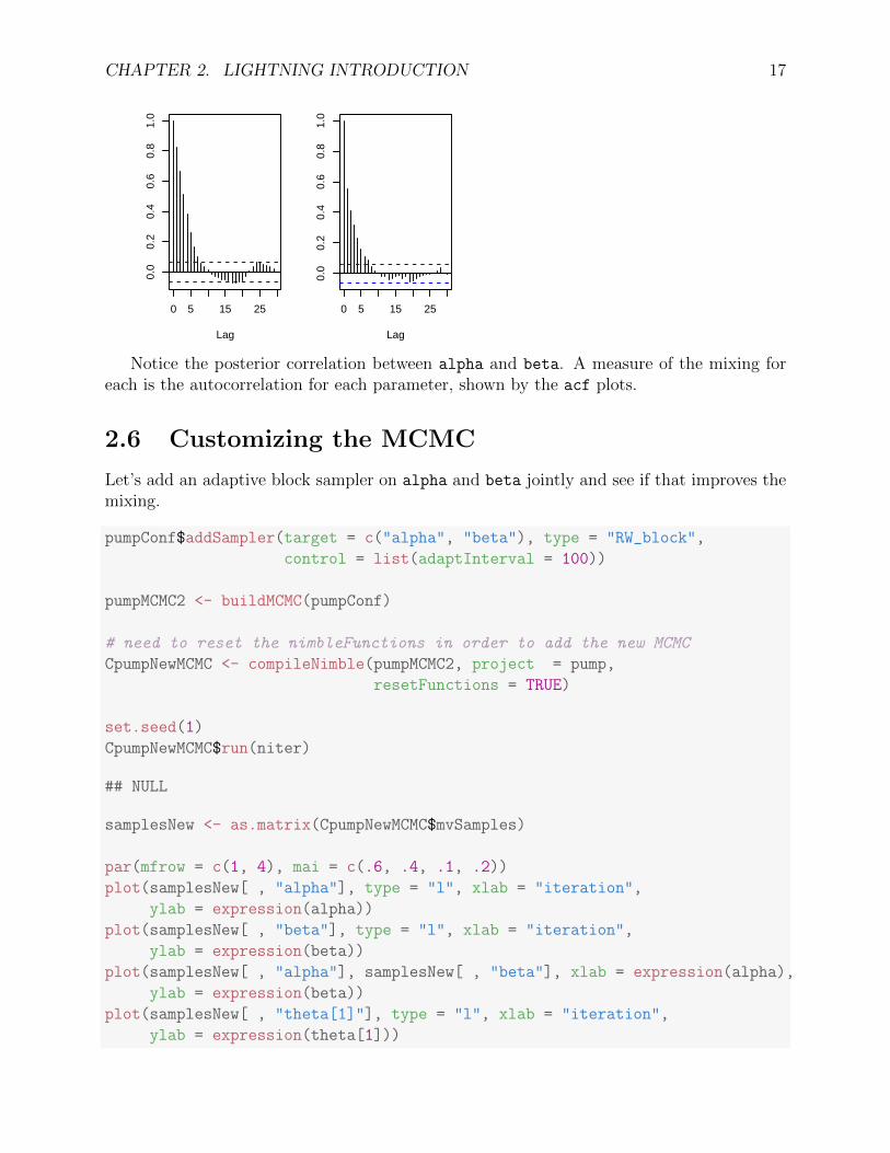
Notice the posterior correlation between alpha and beta. A measure of the mixing foreach is the autocorrelation for each parameter, shown by the acf plots.
2.6 Customizing the MCMC
Let’s add an adaptive block sampler on alpha and beta jointly and see if that improves themixing.
pumpConf$addSampler(target = c("alpha", "beta"), type = "RW_block",
control = list(adaptInterval = 100))
pumpMCMC2 <- buildMCMC(pumpConf)
# need to reset the nimbleFunctions in order to add the new MCMC
CpumpNewMCMC <- compileNimble(pumpMCMC2, project = pump,
resetFunctions = TRUE)
set.seed(1)
CpumpNewMCMC$run(niter)
## NULL
samplesNew <- as.matrix(CpumpNewMCMC$mvSamples)
par(mfrow = c(1, 4), mai = c(.6, .4, .1, .2))
plot(samplesNew[ , "alpha"], type = "l", xlab = "iteration",
ylab = expression(alpha))
plot(samplesNew[ , "beta"], type = "l", xlab = "iteration",
ylab = expression(beta))
plot(samplesNew[ , "alpha"], samplesNew[ , "beta"], xlab = expression(alpha),
ylab = expression(beta))
plot(samplesNew[ , "theta[1]"], type = "l", xlab = "iteration",
ylab = expression(theta[1]))

CHAPTER 2. LIGHTNING INTRODUCTION 18
0 400 800
0.5
1.0
1.5
2.0
iteration
α
0 400 8000
12
3iteration
β
●
●
●
●
●
●
●
●●●
●
●
●
●
●
●●●
●
●●●●
●●
●●
●
●●●
●●●
●
●
●●
●
●
●
●
●●
●
●●
●●
●
●
●
●
●
●
●
●
●●
●
●
●
●
●●
●
●
●●●
●
●
●
●
●●
●
●
●●
●
●●●
●
●
●
●
●
●
●
●
●
●●
●●
●
●
●
●
●●●●
●●●
●
●●
●●
●
●●
●●●●●
●
●
●●
●●
●
●
●
●●
●
●
●●
●
●
●
●
●●●
●
●
●
●●●●
●
●
●
●
●
●
●●●
●●
●
●
●●
●●
●
●
●
●●●
●
●
●●●
●●
●
●●
●
●
●
●
●●●
●
●●
●
●
●●
●
● ●
●
●
●
●●
●●
●
●
●
●
●●
●
●
●
●
●
●
●● ●
●
●
●●
●●
●
●●●
●●
●
●
●
●
●●●●●●
●
●●●●
●
●
●●●
●●
●
●
●
●
●
●
●●
●
●
●
●
●
●
●
●
●
●
●
●
●
●
●●
●●
●
●●●
●
●●
●
●
●
●●
●
●●
●●
●
●
●
●
●
●
●
●
●
●●●●●
●
●
●
●
●
●
●
●
●
●
●●
●
●
●●●
●
●
●●●
●
●
●
●●
●
●●●
●
●
●●
●
●
●
●●●
●●
●
●
●
●
●
●●
●
●●●
●
●●●●●●
●●
●●
●
●●
●
●●
●
●●
● ●
●●
●
●
●
●
●
●
●
●●●●
●
●
●
●
●●●
●
●
●
●
● ●●
●●
●
●●
●
●
●
●
●
●
●●
●
●●
●
●
●●●
●
●
●●●●●
●●
●
●
●
●
●
●
●
●
●
●●
●
●
●
●
●
●
●
●
●
●
●
●
●
●●
●
●●
●
●
●●
●
●●
●
●
●●
●●●
●
●
●
●
●
●
●
●
●
●
●
●
●
●●
●
●●
●
●
●
●
●
●●●●
●●●
●
● ●
●●
●●●●
●●
●
●●●
●
●●
●
●
●●
●
●
●●
●
●
●●
●
●●
●
●●
●●●
●●
●
●●
●
●●
●
●
●
● ●
●
●
●
●●
●●●
●
●
●
●
●
●●
●●●
●
●●
●●
●●
●●●●
●
●
●
●
●●
●
●●
●
●
●●
●
●
●
●
●●●
●
●
●
●
●●●
●
●
●
●
●
●
●●
●
●
●
●
●
●
●
●
●
●
●● ●
●
●
●
●
●●●●●
●
●
●
●
●
●●
●
●●
●●
●● ●
●
●
●
●
●●
●
●●
●
●
●
●
●●
●
●●
●●●
●
●
●●
●
●
●
●
●
●●
●
●●
●
●●
●
●●
●
●●
●
●
●
●●
●
●
●
●
●
●
●
●
●
●
●●
●
●
●
●
●
●
●●
●
●
●
●
●
●
●
●
●
●
●●●●
●
●
●
●
●
●●
●
●
●
●
●●
●●
●●
● ●
●
●●●●
●●
●
●●
●
●●
●
●
●
●
●
●
●
●●
●
●●
●
●
●
●
●
●●
●
●●●●●
●
●●
●●●●
●
●
●●
●
●
●
●●
●●
●●
●
●
●
●●
●
●●
●
●
●
●
●
●●
●●
●
●●●
●●
●
●
●●
●
●
●
●
●
●
●
●●●
●● ●
●
●
●
●
●
●
●●
●
●
●
●●●●●
●●
●
●●
●
●
●
●
●
●
●
●
●●
●
●
●
●
●●
●●●
●
●●●
●
●
●
●
●
● ●●
●
●●
●
●
●●●
●
●
●
●
●
●
●
●
●
●
●
●
●
●
●
●
●
●
●
●
●
●
●●●●●
●●
●
●
●
●●●●
● ●●●●●●
●
●●
●●
●●●●
●
●
●●
●
● ●
●
●●●
●
●
●
●
●
0.5 1.0 1.5 2.0
01
23
α
β
0 400 800
0.05
0.10
0.15
iteration
θ 1
acf(samplesNew[, "alpha"]) ## plot autocorrelation of alpha sample
acf(samplesNew[, "beta"]) ## plot autocorrelation of beta sample
0 5 15 25
0.0
0.2
0.4
0.6
0.8
1.0
Lag
AC
F
0 5 15 25
0.0
0.2
0.4
0.6
0.8
1.0
Lag
AC
F
We can see that the block sampler has decreased the autocorrelation for both alpha andbeta. Of course these are just short runs, and what we are really interested in is the effectivesample size of the MCMC per computation time, but that’s not the point of this example.
Once you learn the MCMC system, you can write your own samplers and include them.The entire system is written in nimbleFunctions.
2.7 Running MCEM
NIMBLE is a system for working with algorithms, not just an MCMC engine. So let’stry maximizing the marginal likelihood for alpha and beta using Monte Carlo ExpectationMaximization2.
pump2 <- pump$newModel()
2Note that for this model, one could analytically integrate over theta and then numerically maximizethe resulting marginal likelihood.

CHAPTER 2. LIGHTNING INTRODUCTION 19
box = list( list(c("alpha","beta"), c(0, Inf)))
pumpMCEM <- buildMCEM(model = pump2, latentNodes = "theta[1:10]",
boxConstraints = box)
# Note: buildMCEM returns an R function that contains a
# nimbleFunction rather than a nimble function. That is why
# pumpMCEM() is used here instead of pumpMCEM£run().
pumpMLE <- pumpMCEM$run()
## Iteration Number: 1.
## Current number of MCMC iterations: 1000.
## Parameter Estimates:
## alpha beta
## 0.8160625 1.1230921
## Convergence Criterion: 1.001.
## Iteration Number: 2.
## Current number of MCMC iterations: 1000.
## Parameter Estimates:
## alpha beta
## 0.8045037 1.1993128
## Convergence Criterion: 0.0223464.
## Monte Carlo error too big: increasing MCMC sample size.
## Iteration Number: 3.
## Current number of MCMC iterations: 1250.
## Parameter Estimates:
## alpha beta
## 0.8203178 1.2497067
## Convergence Criterion: 0.004913688.
## Monte Carlo error too big: increasing MCMC sample size.
## Monte Carlo error too big: increasing MCMC sample size.
## Monte Carlo error too big: increasing MCMC sample size.
## Iteration Number: 4.
## Current number of MCMC iterations: 3032.
## Parameter Estimates:
## alpha beta
## 0.8226618 1.2602452
## Convergence Criterion: 0.0004201048.
pumpMLE
## alpha beta
## 0.8226618 1.2602452

CHAPTER 2. LIGHTNING INTRODUCTION 20
Both estimates are within 0.01 of the values reported by George et al. [8]3. Some dis-crepancy is to be expected since it is a Monte Carlo algorithm.
2.8 Creating your own functions
Now let’s see an example of writing our own algorithm and using it on the model. We’ll dosomething simple: simulating multiple values for a designated set of nodes and calculatingevery part of the model that depends on them. More details on programming in NIMBLEare in Part IV.
Here is our nimbleFunction:
simNodesMany <- nimbleFunction(
setup = function(model, nodes) {mv <- modelValues(model)
deps <- model$getDependencies(nodes)
allNodes <- model$getNodeNames()
},run = function(n = integer()) {
resize(mv, n)
for(i in 1:n) {model$simulate(nodes)
model$calculate(deps)
copy(from = model, nodes = allNodes,
to = mv, rowTo = i, logProb = TRUE)
}})
simNodesTheta1to5 <- simNodesMany(pump, "theta[1:5]")
simNodesTheta6to10 <- simNodesMany(pump, "theta[6:10]")
Here are a few things to notice about the nimbleFunction.
1. The setup function is written in R. It creates relevant information specific to our modelfor use in the run-time code.
2. The setup code creates a modelValues object to hold multiple sets of values for vari-ables in the model provided.
3. The run function is written in NIMBLE. It carries out the calculations using theinformation determined once for each set of model and nodes arguments by the setupcode. The run-time code is what will be compiled.
4. The run code requires type information about the argument n. In this case it is ascalar integer.
5. The for-loop looks just like R, but only sequential integer iteration is allowed.
3Table 2 of the paper accidentally swapped the two estimates.
CHAPTER 2. LIGHTNING INTRODUCTION 21
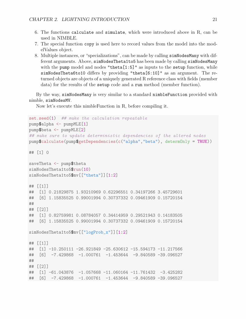
6. The functions calculate and simulate, which were introduced above in R, can beused in NIMBLE.
7. The special function copy is used here to record values from the model into the mod-elValues object.
8. Multiple instances, or “specializations”, can be made by calling simNodesMany with dif-ferent arguments. Above, simNodesTheta1to5 has been made by calling simNodesMany
with the pump model and nodes "theta[1:5]" as inputs to the setup function, whilesimNodesTheta6to10 differs by providing "theta[6:10]" as an argument. The re-turned objects are objects of a uniquely generated R reference class with fields (memberdata) for the results of the setup code and a run method (member function).
By the way, simNodesMany is very similar to a standard nimbleFunction provided withnimble, simNodesMV.
Now let’s execute this nimbleFunction in R, before compiling it.
set.seed(1) ## make the calculation repeatable
pump$alpha <- pumpMLE[1]
pump$beta <- pumpMLE[2]
## make sure to update deterministic dependencies of the altered nodes
pump$calculate(pump$getDependencies(c("alpha","beta"), determOnly = TRUE))
## [1] 0
saveTheta <- pump$theta
simNodesTheta1to5$run(10)
simNodesTheta1to5$mv[["theta"]][1:2]
## [[1]]
## [1] 0.21829875 1.93210969 0.62296551 0.34197266 3.45729601
## [6] 1.15835525 0.99001994 0.30737332 0.09461909 0.15720154
##
## [[2]]
## [1] 0.82759981 0.08784057 0.34414959 0.29521943 0.14183505
## [6] 1.15835525 0.99001994 0.30737332 0.09461909 0.15720154
simNodesTheta1to5$mv[["logProb_x"]][1:2]
## [[1]]
## [1] -10.250111 -26.921849 -25.630612 -15.594173 -11.217566
## [6] -7.429868 -1.000761 -1.453644 -9.840589 -39.096527
##
## [[2]]
## [1] -61.043876 -1.057668 -11.060164 -11.761432 -3.425282
## [6] -7.429868 -1.000761 -1.453644 -9.840589 -39.096527
CHAPTER 2. LIGHTNING INTRODUCTION 22
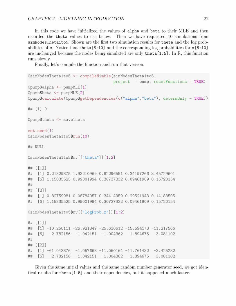
In this code we have initialized the values of alpha and beta to their MLE and thenrecorded the theta values to use below. Then we have requested 10 simulations fromsimNodesTheta1to5. Shown are the first two simulation results for theta and the log prob-abilities of x. Notice that theta[6:10] and the corresponding log probabilities for x[6:10]are unchanged because the nodes being simulated are only theta[1:5]. In R, this functionruns slowly.
Finally, let’s compile the function and run that version.
CsimNodesTheta1to5 <- compileNimble(simNodesTheta1to5,
project = pump, resetFunctions = TRUE)
Cpump$alpha <- pumpMLE[1]
Cpump$beta <- pumpMLE[2]
Cpump$calculate(Cpump$getDependencies(c("alpha","beta"), determOnly = TRUE))
## [1] 0
Cpump$theta <- saveTheta
set.seed(1)
CsimNodesTheta1to5$run(10)
## NULL
CsimNodesTheta1to5$mv[["theta"]][1:2]
## [[1]]
## [1] 0.21829875 1.93210969 0.62296551 0.34197266 3.45729601
## [6] 1.15835525 0.99001994 0.30737332 0.09461909 0.15720154
##
## [[2]]
## [1] 0.82759981 0.08784057 0.34414959 0.29521943 0.14183505
## [6] 1.15835525 0.99001994 0.30737332 0.09461909 0.15720154
CsimNodesTheta1to5$mv[["logProb_x"]][1:2]
## [[1]]
## [1] -10.250111 -26.921849 -25.630612 -15.594173 -11.217566
## [6] -2.782156 -1.042151 -1.004362 -1.894675 -3.081102
##
## [[2]]
## [1] -61.043876 -1.057668 -11.060164 -11.761432 -3.425282
## [6] -2.782156 -1.042151 -1.004362 -1.894675 -3.081102
Given the same initial values and the same random number generator seed, we got iden-tical results for theta[1:5] and their dependencies, but it happened much faster.

Chapter 3
More introduction
Now that we have shown a brief example, we will introduce more about the concepts anddesign of NIMBLE.
One of the most important concepts behind NIMBLE is to allow a combination of high-level processing in R and low-level processing in C++. For example, when we write aMetropolis-Hastings MCMC sampler in the NIMBLE language, the inspection of the modelstructure related to one node is done in R, and the actual sampler calculations are done inC++. This separation between setup and run steps will become clearer as we go.
3.1 NIMBLE adopts and extends the BUGS language
for specifying models
We adopted the BUGS language, and we have extended it to make it more flexible. TheBUGS language became widely used in WinBUGS, then in OpenBUGS and JAGS. Thesesystems all provide automatically-generated MCMC algorithms, but we have adopted onlythe language for describing models, not their systems for generating MCMCs.
NIMBLE extends BUGS by:
1. allowing you to write new functions and distributions and use them in BUGS models;2. allowing you to define multiple models in the same code using conditionals evaluated
when the BUGS code is processed;3. supporting a variety of more flexible syntax such as R-like named parameters and more
general algebraic expressions.
By supporting new functions and distributions, NIMBLE makes BUGS an extensible lan-guage, which is a major departure from previous packages that implement BUGS.
We adopted BUGS because it has been so successful, with over 30,000 users by thetime they stopped counting [12]. Many papers and books provide BUGS code as a way todocument their statistical models. We describe NIMBLE’s version of BUGS later. The websites for WinBUGS, OpenBUGS and JAGS provide other useful documntation on writingmodels in BUGS. For the most part, if you have BUGS code, you can try NIMBLE.
NIMBLE does several things with BUGS code:
23

CHAPTER 3. MORE INTRODUCTION 24
1. NIMBLE creates a model definition object that knows everything about the variablesand their relationships written in the BUGS code. Usually you’ll ignore the modeldefinition and let NIMBLE’s default options take you directly to the next step.
2. NIMBLE creates a model object1. This can be used to manipulate variables andoperate the model from R. Operating the model includes calculating, simulating, orquerying the log probability value of model nodes. These basic capabilities, along withthe tools to query model structure, allow one to write programs that use the modeland adapt to its structure.
3. When you’re ready, NIMBLE can generate customized C++ code representing themodel, compile the C++, load it back into R, and provide a new model object thatuses the compiled model internally. We use the word “compile” to refer to all of thesesteps together.
As an example of how radical a departure NIMBLE is from previous BUGS implemen-tations, consider a situation where you want to simulate new data from a model written inBUGS code. Since NIMBLE creates model objects that you can control from R, simulatingnew data is trivial. With previous BUGS-based packages, this isn’t possible.
More information about specifying and manipulating models is in Chapters 6 and 13.
3.2 nimbleFunctions for writing algorithms
NIMBLE provides nimbleFunctions for writing functions that can (but don’t have to) useBUGS models. The main ways that nimbleFunctions can use BUGS models are:
1. inspecting the structure of a model, such as determining the dependencies betweenvariables, in order to do the right calculations with each model;
2. accessing values of the model’s variables;3. controlling execution of the model’s probability calculations or corresponding simula-
tions;4. managing modelValues data structures for multiple sets of model values and probabil-
ities.
In fact, the calculations of the model are themselves constructed as nimbleFunctions, asare the algorithms provided in NIMBLE’s algorithm library2.
Programming with nimbleFunctions involves a fundamental distinction between two stagesof processing:
1. A setup function within a nimbleFunction gives the steps that need to happen onlyonce for each new situation (e.g., for each new model). Typically such steps includeinspecting the model’s variables and their relationships, such as determining whichparts of a model will need to be calculated for a MCMC sampler. Setup functions areexecuted in R and never compiled.
1or multiple model objects2That’s why it’s easy to use new functions and distributions written as nimbleFunctions in BUGS code.

CHAPTER 3. MORE INTRODUCTION 25
2. One or more run functions within a nimbleFunction give steps that need to happenmultiple times using the results of the setup function, such as the iterations of a MCMCsampler. Formally, run code is written in the NIMBLE language, which you can thinkof as a small subset of R along with features for operating models and related datastructures. The NIMBLE language is what the NIMBLE compiler can automaticallyturn into C++ as part of a compiled nimbleFunction.
What NIMBLE does with a nimbleFunction is similar to what it does with a BUGSmodel:
1. NIMBLE creates a working R version of the nimbleFunction. This is most useful fordebugging (Section 15.7).
2. When you are ready, NIMBLE can generate C++ code, compile it, load it back intoR and give you new objects that use the compiled C++ internally. Again, we refer tothese steps all together as “compilation.” The behavior of compiled nimbleFunctionsis usually very similar, but not identical, to their uncompiled counterparts.
If you are familiar with object-oriented programming, you can think of a nimbleFunctionas a class definition. The setup function initializes a new object and run functions are classmethods. Member data are determined automatically as the objects from a setup functionneeded in run functions. If no setup function is provided, the nimbleFunction correspondsto a simple (compilable) function rather than a class.
More about writing algorithms is in Chapter 15.
3.3 The NIMBLE algorithm library
In Version 0.6-11, the NIMBLE algorithm library includes:
1. MCMC with samplers including conjugate (Gibbs), slice, adaptive random walk (withoptions for reflection or sampling on a log scale), adaptive block random walk, andelliptical slice, among others. You can modify sampler choices and configurations fromR before compiling the MCMC. You can also write new samplers as nimbleFunctions.
2. WAIC calculation for model comparison after an MCMC algorithm has been run.3. A set of particle filter (sequential Monte Carlo) methods including a basic bootstrap
filter, auxiliary particle filter, and Liu-West filter.4. An ascent-based Monte Carlo Expectation Maximization (MCEM) algorithm.5. A variety of basic functions that can be used as programming tools for larger algo-
rithms. These include:
(a) A likelihood function for arbitrary parts of any model.(b) Functions to simulate one or many sets of values for arbitrary parts of any model.(c) Functions to calculate the summed log probability (density) for one or many sets
of values for arbitrary parts of any model along with stochastic dependencies inthe model structure.
More about the NIMBLE algorithm library is in Chapter 8.

Chapter 4
Installing NIMBLE
4.1 Requirements to run NIMBLE
You can run NIMBLE on any of the three common operating systems: Linux, Mac OS X,or Windows.
The following are required to run NIMBLE.
1. R, of course.2. The igraph and coda R packages.3. A working C++ compiler that NIMBLE can use from R on your system. There are
standard open-source C++ compilers that the R community has already made easy toinstall. See Section 4.2 for instructions. You don’t need to know anything about C++to use NIMBLE. This must be done before installing NIMBLE.
NIMBLE also uses a couple of C++ libraries that you don’t need to install, as they willalready be on your system or are provided by NIMBLE.
1. The Eigen C++ library for linear algebra. This comes with NIMBLE, or you can useyour own copy.
2. The BLAS and LAPACK numerical libraries. These come with R, but see Section4.4.3 for how to use a faster version of the BLAS.
Most fairly recent versions of these requirements should work.
4.2 Installing a C++ compiler for NIMBLE to use
NIMBLE needs a C++ compiler and the standard utility make in order to generate andcompile C++ for models and algorithms.1
1This differs from most packages, which might need a C++ compiler only when the package is built. Ifyou normally install R packages using install.packages on Windows or OS X, the package arrives alreadybuilt to your system.
26

CHAPTER 4. INSTALLING NIMBLE 27
4.2.1 OS X
On OS X, you should install Xcode. The command-line tools, which are available as a smallerinstallation, should be sufficient. This is freely available from the Apple developer site andthe App Store.
For the compiler to work correctly for OS X, the installed R must be for the correctversion of OS X. For example, R for Snow Leopard (OS X version 10.8) will attempt to usean incorrect C++ compiler if the installed OS X is actually version 10.9 or higher.
In the somewhat unlikely event you want to install from the source package rather thanthe CRAN binary package, the easiest approach is to use the source package provided atR-nimble.org. If you do want to install from the source package provided by CRAN, you’llneed to install this gfortran package.
4.2.2 Linux
On Linux, you can install the GNU compiler suite (gcc/g++). You can use the packagemanager to install pre-built binaries. On Ubuntu, the following command will install orupdate make, gcc and libc.
sudo apt-get install build-essential
4.2.3 Windows
On Windows, you should download and install Rtools.exe available from http://cran.
r-project.org/bin/windows/Rtools/. Select the appropriate executable correspondingto your version of R (and follow the urge to update your version of R if you notice it is notthe most recent). This installer leads you through several “pages”. We think you can acceptthe defaults with one exception: check the PATH checkbox (page 5) so that the installer willadd the location of the C++ compiler and related tools to your system’s PATH, ensuring thatR can find them. After you click “Next”, you will get a page with a window for customizingthe new PATH variable. You shouldn’t need to do anything there, so you can simply click“Next” again.
The checkbox for the “R 2.15+ toolchain” (page 4) must be checked (in order to havegcc/g++, make, etc. installed). This should be checked by default.
4.3 Installing the NIMBLE package
Since NIMBLE is an R package, you can install it in the usual way, viainstall.packages("nimble") in R or using the R CMD INSTALL method if you downloadthe package source directly.
NIMBLE can also be obtained from the NIMBLE website. To install from our website,please see our Download page for the specific invocation of install.packages.

CHAPTER 4. INSTALLING NIMBLE 28
4.3.1 Problems with installation
We have tested the installation on the three commonly used platforms – OS X, Linux,Windows2. We don’t anticipate problems with installation, but we want to hear about anyand help resolve them. Please post about installation problems to the nimble-users Googlegroup or email [email protected].
4.4 Customizing your installation
For most installations, you can ignore low-level details. However, there are some optionsthat some users may want to utilize.
4.4.1 Using your own copy of Eigen
NIMBLE uses the Eigen C++ template library for linear algebra. Version 3.2.1 of Eigenis included in the NIMBLE package and that version will be used unless the package’sconfiguration script finds another version on the machine. This works well, and the followingis only relevant if you want to use a different (e.g., newer) version.
The configuration script looks in the standard include directories, e.g. /usr/include
and /usr/local/include for the header file Eigen/Dense. You can specify a particularlocation in either of two ways:
1. Set the environment variable EIGEN DIR before installing the R package, e.g., exportEIGEN DIR=/usr/include/eigen3 in the bash shell.
2. UseR CMD INSTALL --configure-args='--with-eigen=/path/to/eigen' \
nimble_VERSION.tar.gz
orinstall.packages("nimble", configure.args = "--with-eigen=/path/to/eigen").
In these cases, the directory should be the full path to the directory that contains the Eigendirectory, e.g., /usr/include/eigen3. It is not the full path to the Eigen directory itself,i.e., NOT /usr/include/eigen3/Eigen.
4.4.2 Using libnimble
NIMBLE generates specialized C++ code for user-specified models and nimbleFunctions.This code uses some NIMBLE C++ library classes and functions. By default, on Linux thelibrary code is compiled once as a linkable library - libnimble.so. This single instance of thelibrary is then linked with the code for each generated model. In contrast, the default forWindows and Mac OS X is to compile the library code as a static library - libnimble.a - thatis compiled into each model’s and each algorithm’s own dynamically loadable library (DLL).This does repeat the same code across models and so occupies more memory. There may bea marginal speed advantage. If one would like to enable the linkable library in place of the
2We’ve tested NIMBLE on Windows 7, 8 and 10.

CHAPTER 4. INSTALLING NIMBLE 29
static library (do this only on Mac OS X and other UNIX variants and not on Windows), onecan install the source package with the configuration argument --enable-dylib set to true.First obtain the NIMBLE source package (which will have the extension .tar.gz from ourwebsite and then install as follows, replacing VERSION with the appropriate version number:
R CMD INSTALL --configure-args='--enable-dylib=true' nimble_VERSION.tar.gz
4.4.3 BLAS and LAPACK
NIMBLE also uses BLAS and LAPACK for some of its linear algebra (in particular cal-culating density values and generating random samples from multivariate distributions).NIMBLE will use the same BLAS and LAPACK installed on your system that R uses. Notethat a fast (and where appropriate, threaded) BLAS can greatly increase the speed of linearalgebra calculations. See Section A.3.1 of the R Installation and Administration manualavailable on CRAN for more details on providing a fast BLAS for your R installation.
4.4.4 Customizing compilation of the NIMBLE-generated C++
For each model or nimbleFunction, NIMBLE can generate and compile C++. To compilegenerated C++, NIMBLE makes system calls starting with R CMD SHLIB and therefore usesthe regular R configuration in ${R_HOME}/etc/${R_ARCH}/Makeconf. NIMBLE places aMakevars file in the directory in which the code is generated, and R CMD SHLIB uses this fileas usual.
In all but specialized cases, the general compilation mechanism will suffice. However,one can customize this. One can specify the location of an alternative Makevars (or Make-vars.win) file to use. Such an alternative file should define the variables PKG CPPFLAGS andPKG LIBS. These should contain, respectively, the pre-processor flag to locate the NIMBLEinclude directory, and the necessary libraries to link against (and their location as necessary),e.g., Rlapack and Rblas on Windows, and libnimble. Advanced users can also change theirdefault compilers by editing the Makevars file, see Section 1.2.1 of the Writing R Extensionsmanual available on CRAN.
Use of this file allows users to specify additional compilation and linking flags. See theWriting R Extensions manual for more details of how this can be used and what it cancontain.

Part II
Models in NIMBLE
30

Chapter 5
Writing models in NIMBLE’s dialectof BUGS
Models in NIMBLE are written using a variation on the BUGS language. From BUGS code,NIMBLE creates a model object. This chapter describes NIMBLE’s version of BUGS. Thenext chapter explains how to build and manipulate model objects.
5.1 Comparison to BUGS dialects supported by Win-
BUGS, OpenBUGS and JAGS
Many users will come to NIMBLE with some familiarity with WinBUGS, OpenBUGS, orJAGS, so we start by summarizing how NIMBLE is similar to and different from those beforedocumenting NIMBLE’s version of BUGS more completely. In general, NIMBLE aims tobe compatible with the original BUGS language and also JAGS’ version. However, at thispoint, there are some features not supported by NIMBLE, and there are some extensionsthat are planned but not implemented.
5.1.1 Supported features of BUGS and JAGS
1. Stochastic and deterministic1 node declarations.2. Most univariate and multivariate distributions.3. Link functions.4. Most mathematical functions.5. “for” loops for iterative declarations.6. Arrays of nodes up to 4 dimensions.7. Truncation and censoring as in JAGS using the T() notation and dinterval.
5.1.2 NIMBLE’s Extensions to BUGS and JAGS
NIMBLE extends the BUGS language in the following ways:
1NIMBLE calls non-stochastic nodes “deterministic”, whereas BUGS calls them “logical”. NIMBLE uses“logical” in the way R does, to refer to boolean (TRUE/FALSE) variables.
31
CHAPTER 5. WRITING MODELS IN NIMBLE’S DIALECT OF BUGS 32
1. User-defined functions and distributions – written as nimbleFunctions – can be usedin model code. See Chapter 12.
2. Multiple parameterizations for distributions, similar to those in R, can be used.3. Named parameters for distributions and functions, similar to R function calls, can be
used.4. Linear algebra, including for vectorized calculations of simple algebra, can be used in
deterministic declarations.5. Distribution parameters can be expressions, as in JAGS but not in WinBUGS. Caveat:
parameters to multivariate distributions (e.g., dmnorm) cannot be expressions (but anexpression can be defined in a separate deterministic expression and the resultingvariable then used).
6. Alternative models can be defined from the same model code by using if-then-elsestatements that are evaluated when the model is defined.
7. More flexible indexing of vector nodes within larger variables is allowed. For exampleone can place a multivariate normal vector arbitrarily within a higher-dimensionalobject, not just in the last index.
8. More general constraints can be declared using dconstraint, which extends the con-cept of JAGS’ dinterval.
9. Link functions can be used in stochastic, as well as deterministic, declarations.2
10. Data values can be reset, and which parts of a model are flagged as data can bechanged, allowing one model to be used for different data sets without rebuilding themodel each time.
11. As of Version 0.6-6 we now support stochastic/dynamic indexes. More specifically inearlier versions all indexes needed to be constants. Now indexes can be other nodes orfunctions of other nodes. For a given dimension of a node being indexed, if the indexis not constant, it must be a scalar value. So expressions such as mu[k[i], 3] ormu[k[i], 1:3] or mu[k[i], j[i]] are allowed, but not mu[k[i]:(k[i]+1)]. Nesteddynamic indexes such as mu[k[j[i]]] are also allowed.
5.1.3 Not-yet-supported features of BUGS and JAGS
In this release, the following are not supported.
1. The appearance of the same node on the left-hand side of both a <- and a ∼ declaration(used in WinBUGS for data assignment for the value of a stochastic node).
2. Multivariate nodes must appear with brackets, even if they are empty. E.g., x cannotbe multivariate but x[] or x[2:5] can be.
3. NIMBLE generally determines the dimensionality and sizes of variables from the BUGScode. However, when a variable appears with blank indices, such as in x.sum <-
sum(x[]), and if the dimensions of the variable are not clearly defined in other dec-larations, NIMBLE currently requires that the dimensions of x be provided when themodel object is created (via nimbleModel).
2But beware of the possibility of needing to set values for “lifted” nodes created by NIMBLE.

CHAPTER 5. WRITING MODELS IN NIMBLE’S DIALECT OF BUGS 33
5.2 Writing models
Here we introduce NIMBLE’s version of BUGS. The WinBUGS, OpenBUGS and JAGSmanuals are also useful resources for writing BUGS models, including many examples.
5.2.1 Declaring stochastic and deterministic nodes
BUGS is a declarative language for graphical (or hierarchical) models. Most programminglanguages are imperative, which means a series of commands will be executed in the orderthey are written. A declarative language like BUGS is more like building a machine beforeusing it. Each line declares that a component should be plugged into the machine, butit doesn’t matter in what order they are declared as long as all the right components areplugged in by the end of the code.
The machine in this case is a graphical model3. A node (sometimes called a vertex ) holdsone value, which may be a scalar or a vector. Edges define the relationships between nodes.A huge variety of statistical models can be thought of as graphs.
Here is the code to define and create a simple linear regression model with four observa-tions.
library(nimble)
mc <- nimbleCode({intercept ~ dnorm(0, sd = 1000)
slope ~ dnorm(0, sd = 1000)
sigma ~ dunif(0, 100)
for(i in 1:4) {predicted.y[i] <- intercept + slope * x[i]
y[i] ~ dnorm(predicted.y[i], sd = sigma)
}})
model <- nimbleModel(mc, data = list(y = rnorm(4)))
library(igraph)
layout <- matrix(ncol = 2, byrow = TRUE,
## These seem to be rescaled to fit in the plot area,
## so I'll just use 0-100 as the scale
data = c(33, 100,
66, 100,
50, 0, ## first three are parameters
15, 50, 35, 50, 55, 50, 75, 50, ## x's
20, 75, 40, 75, 60, 75, 80, 75, ## predicted.y's
25, 25, 45, 25, 65, 25, 85, 25) ## y's
3Technically, a directed acyclic graph

CHAPTER 5. WRITING MODELS IN NIMBLE’S DIALECT OF BUGS 34
)
sizes <- c(45, 30, 30,
rep(20, 4),
rep(50, 4),
rep(20, 4))
edge.color <- "black"
## c(
## rep("green", 8),
## rep("red", 4),
## rep("blue", 4),
## rep("purple", 4))
stoch.color <- "deepskyblue2"
det.color <- "orchid3"
rhs.color <- "gray73"
fill.color <- c(
rep(stoch.color, 3),
rep(rhs.color, 4),
rep(det.color, 4),
rep(stoch.color, 4)
)
plot(model$graph, vertex.shape = "crectangle",
vertex.size = sizes,
vertex.size2 = 20,
layout = layout,
vertex.label.cex = 3.0,
vertex.color = fill.color,
edge.width = 3,
asp = 0.5,
edge.color = edge.color)
The graph representing the model is shown in Figure 5.1. Each observation, y[i], is anode whose edges say that it follows a normal distribution depending on a predicted value,predicted.y[i], and standard deviation, sigma, which are each nodes. Each predictedvalue is a node whose edges say how it is calculated from slope, intercept, and one valueof an explanatory variable, x[i], which are each nodes.
This graph is created from the following BUGS code:
{intercept ~ dnorm(0, sd = 1000)
slope ~ dnorm(0, sd = 1000)

CHAPTER 5. WRITING MODELS IN NIMBLE’S DIALECT OF BUGS 35
intercept slope
sigma
x[1] x[2] x[3] x[4]
predicted.y[1] predicted.y[2] predicted.y[3] predicted.y[4]
y[1] y[2] y[3] y[4]
Figure 5.1: Graph of a linear regression model
sigma ~ dunif(0, 100)
for(i in 1:4) {predicted.y[i] <- intercept + slope * x[i]
y[i] ~ dnorm(predicted.y[i], sd = sigma)
}}
In this code, stochastic relationships are declared with “∼” and deterministic relation-ships are declared with “<-”. For example, each y[i] follows a normal distribution withmean predicted.y[i] and standard deviation sigma. Each predicted.y[i] is the resultof intercept + slope * x[i]. The for-loop yields the equivalent of writing four lines ofcode, each with a different value of i. It does not matter in what order the nodes aredeclared. Imagine that each line of code draws part of Figure 5.1, and all that matters isthat the everything gets drawn in the end. Available distributions, default and alternativeparameterizations, and functions are listed in Section 5.2.4.
An equivalent graph can be created by this BUGS code:
{intercept ~ dnorm(0, sd = 1000)
slope ~ dnorm(0, sd = 1000)
sigma ~ dunif(0, 100)
for(i in 1:4) {y[i] ~ dnorm(intercept + slope * x[i], sd = sigma)
}}

CHAPTER 5. WRITING MODELS IN NIMBLE’S DIALECT OF BUGS 36
In this case, the predicted.y[i] nodes in Figure 5.1 will be created automatically byNIMBLE and will have a different name, generated by NIMBLE.
5.2.2 More kinds of BUGS declarations
Here are some examples of valid lines of BUGS code. This code does not describe a sensibleor complete model, and it includes some arbitrary indices (e.g. mvx[8:10, i]) to illustrateflexibility. Instead the purpose of each line is to illustrate a feature of NIMBLE’s version ofBUGS.
{## 1. normal distribution with BUGS parameter order
x ~ dnorm(a + b * c, tau)
## 2. normal distribution with a named parameter
y ~ dnorm(a + b * c, sd = sigma)
## 3. For-loop and nested indexing
for(i in 1:N) {for(j in 1:M[i]) {
z[i,j] ~ dexp(r[ blockID[i] ])
}}## 4. multivariate distribution with arbitrary indexing
for(i in 1:3)
mvx[8:10, i] ~ dmnorm(mvMean[3:5], cov = mvCov[1:3, 1:3, i])
## 5. User-provided distribution
w ~ dMyDistribution(hello = x, world = y)
## 6. Simple deterministic node
d1 <- a + b
## 7. Vector deterministic node with matrix multiplication
d2[] <- A[ , ] %*% mvMean[1:5]
## 8. Deterministic node with user-provided function
d3 <- foo(x, hooray = y)
}
When a variable appears only on the right-hand side, it can be provided via constants
(in which case it can never be changed) or via data or inits, as discussed in Chapter 6.Notes on the comment-numbered lines are:
1. x follows a normal distribution with mean a + b*c and precision tau (default BUGSsecond parameter for dnorm).
2. y follows a normal distribution with the same mean as x but a named standard devi-ation parameter instead of a precision parameter (sd = 1/sqrt(precision)).
3. z[i, j] follows an exponential distribution with parameter r[ blockID[i] ]. Thisshows how for-loops can be used for indexing of variables containing multiple nodes.Variables that define for-loop indices (N and M) must also be provided as constants.

CHAPTER 5. WRITING MODELS IN NIMBLE’S DIALECT OF BUGS 37
4. The arbitrary block mvx[8:10, i] follows a multivariate normal distribution, with anamed covariance matrix instead of BUGS’ default of a precision matrix. As in R,curly braces for for-loop contents are only needed if there is more than one line.
5. w follows a user-defined distribution. See Chapter 12.6. d1 is a scalar deterministic node that, when calculated, will be set to a + b.7. d2 is a vector deterministic node using matrix multiplication in R’s syntax.8. d3 is a deterministic node using a user-provided function. See Chapter 12.
More about indexing
Examples of allowed indexing include:
• x[i] # a single index• x[i:j] # a range of indices• x[i:j,k:l] # multiple single indices or ranges for higher-dimensional arrays• x[i:j, ] # blank indices indicating the full range• x[3*i+7] # computed indices• x[(3*i):(5*i+1)] # computed lower and upper ends of an index range• x[k[i]+1] # a dynamic (and computed) index• x[k[j[i]]] # nested dynamic indexes• x[k[i], 1:3] # nested indexing of rows or columns
NIMBLE does not allow multivariate nodes to be used without square brackets, which isan incompatibility with JAGS. Therefore a statement like xbar <- mean(x) in JAGS mustbe converted to xbar <- mean(x[]) (if x is a vector) or xbar <- mean(x[,]) (if x is amatrix) for NIMBLE4. Section 6.1.1 discusses how to provide NIMBLE with dimensions ofx when needed.
Generally NIMBLE supports R-like linear algebra expressions and attempts to followthe same rules as R about dimensions (although in some cases this is not possible). Forexample, x[1:3] %*% y[1:3] converts x[1:3] into a row vector and thus computes theinner product, which is returned as a 1 × 1 matrix (use inprod to get it as a scalar, whichit typically easier). Like in R, a scalar index will result in dropping a dimension unlessthe argument drop=FALSE is provided. For example, mymatrix[i, 1:3] will be a vector oflength 3, but mymatrix[i, 1:3, drop=FALSE] will be a 1× 3 matrix. More about indexingand dimensions is discussed in Section 11.3.2.
5.2.3 Vectorized versus scalar declarations
Suppose you need nodes logY[i] that should be the log of the corresponding Y[i], say fori from 1 to 10. Conventionally this would be created with a for loop:
{for(i in 1:10) {
4In nimbleFunctions explained in later chapters, square brackets with blank indices are not necessaryfor multivariate objects.

CHAPTER 5. WRITING MODELS IN NIMBLE’S DIALECT OF BUGS 38
logY[i] <- log(Y[i])
}}
Since NIMBLE supports R-like algebraic expressions, an alternative in NIMBLE’s dialectof BUGS is to use a vectorized declaration like this:
{logY[1:10] <- log(Y[1:10])
}
There is an important difference between the models that are created by the above twomethods. The first creates 10 scalar nodes, logY[1] , . . . , logY[10]. The second createsone vector node, logY[1:10]. If each logY[i] is used separately by an algorithm, it may bemore efficient computationally if they are declared as scalars. If they are all used together,it will often make sense to declare them as a vector.
5.2.4 Available distributions
Distributions
NIMBLE supports most of the distributions allowed in BUGS and JAGS. Table 5.1 liststhe distributions that are currently supported, with their default parameterizations, whichmatch those of BUGS5. NIMBLE also allows one to use alternative parameterizations fora variety of distributions as described next. See Section 12.2 to learn how to write newdistributions using nimbleFunctions.
Table 5.1: Distributions with their default order of parameters. The value of the random variableis denoted by x.
Name Usage Density Lower Upper
Bernoulli dbern(prob = p)px(1− p)1−x 0 1
0 < p < 1Beta dbeta(shape1 = a, xa−1(1− x)b−1
β(a, b)0 1
shape2 = b), a > 0, b > 0Binomial dbin(prob = p, size = n) (
nx
)px(1− p)n−x 0 n
0 < p < 1, n ∈ N∗Intrinsic dcar normal(adj, weights,
see chapter 9 for detailsCAR num, tau, c, zero mean)
Categorical dcat(prob = p) px∑i pi
1 Np ∈ (R+)N
Chi-square dchisq(df = k) xk2−1 exp(−x/2)
2k2 Γ( k
2)
0
5Note that the same distributions are available for writing nimbleFunctions, but in that case the defaultparameterizations and function names match R’s when possible. Please see Section 11.2.4 for how to usedistributions in nimbleFunctions.

CHAPTER 5. WRITING MODELS IN NIMBLE’S DIALECT OF BUGS 39
Table 5.1: Distributions with their default order of parameters. The value of the random variableis denoted by x.
Name Usage Density Lower Upper
k > 0Dirichlet ddirch(alpha = α)
Γ(∑
i αi)∏j
xαj−1j
Γ(αj)
0αj ≥ 0
Exponential dexp(rate = λ)λ exp(−λx)
0λ > 0
Flat dflat() ∝ 1 (improper)Gamma dgamma(shape = r, rate = λ) λrxr−1 exp(−λx)
Γ(r)0
λ > 0, r > 0Half flat dhalfflat() ∝ 1 (improper) 0Inverse dinvgamma(shape = r, λrx−(r+1) exp(−λ/x)
Γ(r)
0Gamma scale = λ), λ > 0, r > 0Logistic dlogis(location = µ, τ exp{(x− µ)τ}
[1 + exp{(x− µ)τ}]2rate = τ), τ > 0Log-normal dlnorm(meanlog = µ, (
τ2π
) 12 x−1 exp
{−τ(log(x)− µ)2/2
} 0taulog = τ), τ > 0
Multinomial dmulti(prob = p, size = n)n!∏j
pxjj
xj !∑
j xj = n
Multivariate dmnorm(mean = µ, prec = Λ)(2π)−
d2 |Λ|
12 exp{− (x−µ)TΛ(x−µ)
2 }normal Λ positive definiteMultivariate dmvt(mu = µ, prec = Λ, Γ( ν+d
2)
Γ( ν2
)(νπ)d/2|Λ|1/2(1 + (x−µ)TΛ(x−µ)
ν )−ν+d2
Student t df = ν), Λ positive definiteNegative dnegbin(prob = p, size = r) (
x+r−1x
)pr(1− p)x 0
binomial 0 < p ≤ 1, r ≥ 0Normal dnorm(mean = µ, tau = τ) (
τ2π
) 12 exp{−τ(x− µ)2/2}τ > 0
Poisson dpois(lambda = λ) exp(−λ)λx
x!
0λ > 0
Student t dt(mu = µ, tau = τ, df = k) Γ( k+12
)
Γ( k2
)
(τkπ
) 12
{1 + τ(x−µ)2
k
}− (k+1)2
τ > 0, k > 0Uniform dunif(min = a, max = b) 1
b− aa b
a < bWeibull dweib(shape = v, lambda = λ)
vλxv−1 exp(−λxv) 0v > 0, λ > 0
Wishart dwish(R = R, df = k) |x|(k−p−1)/2|R|k/2 exp{−tr(Rx)/2}2pk/2πp(p−1)/4
∏i=1 pΓ((k + 1− i)/2)R p× p pos. def., k ≥ p
Inverse dinvwish(S = S, df = k) |x|−(k+p+1)/2|S|k/2 exp{−tr(Sx−1)/2}2pk/2πp(p−1)/4
∏i=1 pΓ((k + 1− i)/2)Wishart S p× p pos. def., k ≥ p
Improper distributions Note that dcar normal, dflat and dhalfflat specify improperprior distributions and should only be used when the posterior distribution of the model is

CHAPTER 5. WRITING MODELS IN NIMBLE’S DIALECT OF BUGS 40
known to be proper. Also for these distributions, the density function returns the unnor-malized density and the simulation function returns NaN so these distributions are not ap-propriate for algorithms that need to simulate from the prior or require proper (normalized)densities.
Alternative parameterizations for distributions
NIMBLE allows one to specify distributions in model code using a variety of parameteri-zations, including the BUGS parameterizations. Available parameterizations are listed inTable 5.2. To understand how NIMBLE handles alternative parameterizations, it is usefulto distinguish three cases, using the gamma distribution as an example:
1. A canonical parameterization is used directly for computations6. For gamma, this is(shape, scale).
2. The BUGS parameterization is the one defined in the original BUGS language. In gen-eral this is the parameterization for which conjugate MCMC samplers can be executedmost efficiently. For gamma, this is (shape, rate).
3. An alternative parameterization is one that must be converted into the canonical pa-rameterization. For gamma, NIMBLE provides both (shape, rate) and (mean, sd) pa-rameterization and creates nodes to calculate (shape, scale) from either (shape, rate)or (mean, sd). In the case of gamma, the BUGS parameterization is also an alternativeparameterization.
Since NIMBLE provides compatibility with existing BUGS and JAGS code, the order ofparameters places the BUGS parameterization first. For example, the order of parametersfor dgamma is dgamma(shape, rate, scale, mean, sd). Like R, if parameter names arenot given, they are taken in order, so that (shape, rate) is the default. This happens tomatch R’s order of parameters, but it need not. If names are given, they can be given inany order. NIMBLE knows that rate is an alternative to scale and that (mean, sd) are analternative to (shape, scale or rate).
Table 5.2: Distribution parameterizations allowed in NIMBLE. The first column indicatesthe supported parameterizations for distributions given in Table 5.1. The second columnindicates the relationship to the canonical parameterization used in NIMBLE.
Parameterization NIMBLE re-parameterization
dbern(prob) dbin(size = 1, prob)
dbeta(shape1, shape2) canonicaldbeta(mean, sd) dbeta(shape1 = mean^2 * (1-mean) / sd^2 - mean,
shape2 = mean * (1 - mean)^2 / sd^2 + mean - 1)
dbin(prob, size) canonicaldcat(prob) canonicaldchisq(df) canonicalddirch(alpha) canonical
6Usually this is the parameterization in the Rmath header of R’s C implementation of distributions.

CHAPTER 5. WRITING MODELS IN NIMBLE’S DIALECT OF BUGS 41
Table 5.2: Distribution parameterizations allowed in NIMBLE. The first column indicatesthe supported parameterizations for distributions given in Table 5.1. The second columnindicates the relationship to the canonical parameterization used in NIMBLE.
Parameterization NIMBLE re-parameterization
dexp(rate) canonicaldexp(scale) dexp(rate = 1/scale)
dgamma(shape, scale) canonicaldgamma(shape, rate) dgamma(shape, scale = 1 / rate)
dgamma(mean, sd) dgamma(shape = mean^2/sd^2, scale = sd^2/mean)
dinvgamma(shape, rate) canonicaldinvgamma(shape, scale) dgamma(shape, rate = 1 / scale)
dlogis(location, scale) canonicaldlogis(location, rate) dlogis(location, scale = 1 / rate
dlnorm(meanlog, sdlog) canonicaldlnorm(meanlog, taulog) dlnorm(meanlog, sdlog = 1 / sqrt(taulog)
dlnorm(meanlog, varlog) dlnorm(meanlog, sdlog = sqrt(varlog)
dmulti(prob, size) canonicaldmnorm(mean, cholesky, canonical (precision)
prec param=1)
dmnorm(mean, cholesky, canonical (covariance)prec param=0)
dmnorm(mean, prec) dmnorm(mean, cholesky = chol(prec), prec param=1)
dmnorm(mean, cov) dmnorm(mean, cholesky = chol(cov), prec param=0)
dmvt(mu, cholesky, df, canonical (precision/inverse scale)prec param=1)
dmvt(mu, cholesky, df, canonical (scale)prec param=0)
dmvt(mu, prec, df) dmvt(mu, cholesky = chol(prec), df, prec param=1)
dmvt(mu, scale, df) dmvt(mu, cholesky = chol(scale), df, prec param=0)
dnegbin(prob, size) canonicaldnorm(mean, sd) canonicaldnorm(mean, tau) dnorm(mean, sd = 1 / sqrt(var))
dnorm(mean, var) dnorm(mean, sd = sqrt(var))
dpois(lambda) canonicaldt(mu, sigma, df) canonicaldt(mu, tau, df) dt(mu, sigma = 1 / sqrt(tau), df)
dt(mu, sigma2, df) dt(mu, sigma = sqrt(sigma2), df)
dunif(min, max) canonicaldweib(shape, scale) canonicaldweib(shape, rate) dweib(shape, scale = 1 / rate)
dweib(shape, lambda) dweib(shape, scale = lambda^(- 1 / shape)
dwish(cholesky, df) canonical (scale)scale param=1)
dwish(cholesky, df) canonical (inverse scale)

CHAPTER 5. WRITING MODELS IN NIMBLE’S DIALECT OF BUGS 42
Table 5.2: Distribution parameterizations allowed in NIMBLE. The first column indicatesthe supported parameterizations for distributions given in Table 5.1. The second columnindicates the relationship to the canonical parameterization used in NIMBLE.
Parameterization NIMBLE re-parameterization
scale param=0)
dwish(R, df) dwish(cholesky = chol(R), df, scale param = 0)
dwish(S, df) dwish(cholesky = chol(S), df, scale param = 1)
dinvwish(cholesky, df) canonical (scale)scale param=1)
dinvwish(cholesky, df) canonical (inverse scale)scale param=0)
dinvwish(R, df) dinvwish(cholesky = chol(R), df, scale param = 0)
dinvwish(S, df) dinvwish(cholesky = chol(S), df, scale param = 1)
Note that for multivariate normal, multivariate t, Wishart, and Inverse Wishart, thecanonical parameterization uses the Cholesky decomposition of one of the precision/inversescale or covariance/scale matrix. For example, for the multivariate normal, if prec param=TRUE,the cholesky argument is treated as the Cholesky decomposition of a precision matrix. Oth-erwise it is treated as the Cholesky decomposition of a covariance matrix.
In addition, NIMBLE supports alternative distribution names, known as aliases, as inJAGS, as specified in Table 5.3.
Distribution Canonical name AliasBinomial dbin dbinomChi-square dchisq dchisqrDirichlet ddirch ddirichMultinomial dmulti dmultinomNegative binomial dnegbin dnbinomWeibull dweib dweibullWishart dwish dwishart
Table 5.3: Distributions with alternative names (aliases).

CHAPTER 5. WRITING MODELS IN NIMBLE’S DIALECT OF BUGS 43
We plan to, but do not currently, include the following distributions as part of coreNIMBLE: double exponential (Laplace), beta-binomial, Dirichlet-multinomial, F, Pareto, orforms of the multivariate t other than the standard one provided.
5.2.5 Available BUGS language functions
Tables 5.4-5.5 show the available operators and functions. Support for more general Rexpressions is covered in Chapter 11 about programming with nimbleFunctions.
For the most part NIMBLE supports the functions used in BUGS and JAGS, with ex-ceptions indicated in the table. Additional functions provided by NIMBLE are also listed.Note that we provide distribution functions for use in calculations, namely the “p”, “q”, and“d” functions. See Section 11.2.4 for details on the syntax for using distribution functions asfunctions in deterministic calculations, as only some parameterizations are allowed and thenames of some distributions differ from those used to define stochastic nodes in a model.
Table 5.4: Functions operating on scalars, many of which can operate on each element (component-wise) ofvectors and matrices. Status column indicates if the function is currently provided in NIMBLE.
Usage Description Comments Status Acceptsvector input
x | y, x & y logical OR (|) and AND(&) ! !
!x logical not ! !
x > y, x >= y greater than (and or equal to) ! !
x < y, x <= y less than (and or equal to) ! !
x != y, x == y (not) equals ! !
x + y, x - y, x * y component-wise operators mix of scalar and vector ok ! !
x / y, component-wise division vector x and scalar y ok ! !
x^y, pow(x, y) power xy; vector x and scalar y ok ! !
x %% y modulo (remainder) !
min(x1, x2), min. (max.) of two scalars ! See pmin, pmaxmax(x1, x2)
exp(x) exponential ! !
log(x) natural logarithm ! !
sqrt(x) square root ! !
abs(x) absolute value ! !
step(x) step function at 0 0 if x < 0, 1 if x >= 0 ! !
equals(x, y) equality of two scalars 1 if x == y, 0 if x! = y !
cube(x) third power x3 ! !
sin(x), cos(x), tan(x) trigonometric functions ! !
asin(x), acos(x), inverse trigonometric functions ! !atan(x)
asinh(x), acosh(x), inv. hyperbolic trig. functions ! !atanh(x)
logit(x) logit log(x/(1− x)) ! !
ilogit(x), expit(x) inverse logit exp(x)/(1 + exp(x)) ! !
probit(x) probit (Gaussian quantile) Φ−1(x) ! !
iprobit(x), phi(x) inverse probit (Gaussian CDF) Φ(x) ! !
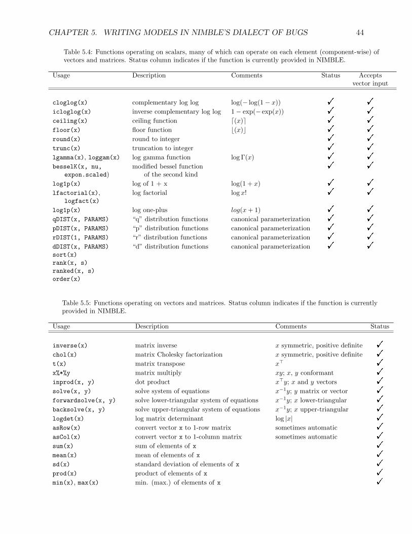
CHAPTER 5. WRITING MODELS IN NIMBLE’S DIALECT OF BUGS 44
Table 5.4: Functions operating on scalars, many of which can operate on each element (component-wise) ofvectors and matrices. Status column indicates if the function is currently provided in NIMBLE.
Usage Description Comments Status Acceptsvector input
cloglog(x) complementary log log log(− log(1− x)) ! !
icloglog(x) inverse complementary log log 1− exp(− exp(x)) ! !
ceiling(x) ceiling function d(x)e ! !
floor(x) floor function b(x)c ! !
round(x) round to integer ! !
trunc(x) truncation to integer ! !
lgamma(x), loggam(x) log gamma function log Γ(x) ! !
besselK(x, nu, modified bessel function ! !expon.scaled) of the second kind
log1p(x) log of 1 + x log(1 + x) ! !
lfactorial(x), log factorial log x! ! !logfact(x)
log1p(x) log one-plus log(x+ 1) ! !
qDIST(x, PARAMS) “q” distribution functions canonical parameterization ! !
pDIST(x, PARAMS) “p” distribution functions canonical parameterization ! !
rDIST(1, PARAMS) “r” distribution functions canonical parameterization ! !
dDIST(x, PARAMS) “d” distribution functions canonical parameterization ! !sort(x)
rank(x, s)
ranked(x, s)
order(x)
Table 5.5: Functions operating on vectors and matrices. Status column indicates if the function is currentlyprovided in NIMBLE.
Usage Description Comments Status
inverse(x) matrix inverse x symmetric, positive definite !
chol(x) matrix Cholesky factorization x symmetric, positive definite !
t(x) matrix transpose x> !
x%*%y matrix multiply xy; x, y conformant !
inprod(x, y) dot product x>y; x and y vectors !
solve(x, y) solve system of equations x−1y; y matrix or vector !
forwardsolve(x, y) solve lower-triangular system of equations x−1y; x lower-triangular !
backsolve(x, y) solve upper-triangular system of equations x−1y; x upper-triangular !
logdet(x) log matrix determinant log |x| !
asRow(x) convert vector x to 1-row matrix sometimes automatic !
asCol(x) convert vector x to 1-column matrix sometimes automatic !
sum(x) sum of elements of x !
mean(x) mean of elements of x !
sd(x) standard deviation of elements of x !
prod(x) product of elements of x !
min(x), max(x) min. (max.) of elements of x !
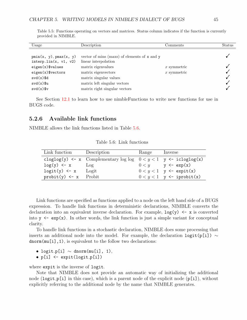
CHAPTER 5. WRITING MODELS IN NIMBLE’S DIALECT OF BUGS 45
Table 5.5: Functions operating on vectors and matrices. Status column indicates if the function is currentlyprovided in NIMBLE.
Usage Description Comments Status
pmin(x, y), pmax(x, y) vector of mins (maxs) of elements of x and y !interp.lin(x, v1, v2) linear interpolation
eigen(x)$values matrix eigenvalues x symmetric !
eigen(x)$vectors matrix eigenvectors x symmetric !
svd(x)$d matrix singular values !
svd(x)$u matrix left singular vectors !
svd(x)$v matrix right singular vectors !
See Section 12.1 to learn how to use nimbleFunctions to write new functions for use inBUGS code.
5.2.6 Available link functions
NIMBLE allows the link functions listed in Table 5.6.
Table 5.6: Link functions
Link function Description Range Inverse
cloglog(y) <- x Complementary log log 0 < y < 1 y <- icloglog(x)
log(y) <- x Log 0 < y y <- exp(x)
logit(y) <- x Logit 0 < y < 1 y <- expit(x)
probit(y) <- x Probit 0 < y < 1 y <- iprobit(x)
Link functions are specified as functions applied to a node on the left hand side of a BUGSexpression. To handle link functions in deterministic declarations, NIMBLE converts thedeclaration into an equivalent inverse declaration. For example, log(y) <- x is convertedinto y <- exp(x). In other words, the link function is just a simple variant for conceptualclarity.
To handle link functions in a stochastic declaration, NIMBLE does some processing thatinserts an additional node into the model. For example, the declaration logit(p[i]) ∼dnorm(mu[i],1), is equivalent to the follow two declarations:
• logit p[i] ∼ dnorm(mu[i], 1),• p[i] <- expit(logit p[i])
where expit is the inverse of logit.Note that NIMBLE does not provide an automatic way of initializing the additional
node (logit p[i] in this case), which is a parent node of the explicit node (p[i]), withoutexplicitly referring to the additional node by the name that NIMBLE generates.

CHAPTER 5. WRITING MODELS IN NIMBLE’S DIALECT OF BUGS 46
5.2.7 Truncation, censoring, and constraints
NIMBLE provides three ways to declare boundaries on the value of a variable, each for dif-ferent situations. We introduce these and comment on their relationships to related featuresof JAGS and BUGS. The three methods are:
Truncation
Either of the following forms,
• x ∼ dnorm(0, sd = 10) T(0, a), or• x ∼ T(dnorm(0, sd = 10), 0, a),
declares that x follows a normal distribution between 0 and a (inclusive of 0 and a). Eitherboundary may be omitted or may be another node, such as a in this example. The first formis compatible with JAGS, but in NIMBLE it can only be used when reading code from atext file. When writing model code in R, the second version must be used.
Truncation means the possible values of x are limited a priori, hence the probabilitydensity of x must be normalized7. In this example it would be the normal probability densitydivided by its integral from 0 to a. Like JAGS, NIMBLE also provides I as a synonym forT to accommodate older BUGS code, but T is preferred because it disambiguates multipleusages of I in BUGS.
Censoring
Censoring refers to the situation where one datum gives the lower or upper bound on anunobserved random variable. This is common in survival analysis, when for an individualstill surviving at the end of a study, the age of death is not known and hence is “censored”(right-censoring). NIMBLE adopts JAGS syntax for censoring, as follows:
censored[i] ~ dinterval(t[i], c[i])
t[i] ~ dweib(r, mu[i])
In the case of right-censoring, censored[i] should be given as data with a value of1 if t[i] is right-censored (t[i] > c[i]) and 0 if it is observed. The data vector for t
should have NA (indicating missing data) for any censored t[i] entries. (As a result, thesenodes will be sampled in an MCMC.) The data vector for c should give the censoring timescorresponding to censored entries and a value above the observed times for uncensored entries(e.g., Inf). Left-censored observations would be specified by setting censored[i] to 0 andt[i] to NA.
The dinterval is not really a distribution but rather a trick: in the above examplewhen censored[i] = 1 it gives a “probability” of 1 if t[i] > c[i] and 0 otherwise. Thismeans that t[i] ≤ c[i] is treated as impossible. More generally than simple right- orleft-censoring, censored[i] ∼ dinterval(t[i], c[i, ]) is defined such that for a vector
7NIMBLE uses the CDF and inverse CDF (quantile) functions of a distribution to do this; in some casesif one uses truncation to include only the extreme tail of a distribution, numerical difficulties can arise.

CHAPTER 5. WRITING MODELS IN NIMBLE’S DIALECT OF BUGS 47
of increasing cutpoints, c[i, ], t[i] is enforced to fall within the censored[i]-th cutpointinterval. This is done by setting data censored[i] as follows:
censored[i] = 0 if t[i] ≤ c[i, 1]
censored[i] = m if c[i, m] < t[i] ≤ c[i, m+1] for 1 <= m <= M
censored[i] = M if c[i, M] < t[i].
(The i index is provided only for consistency with the previous example.) The most commonuses of dinterval will be for left- and right-censored data, in which case c[i,] will be asingle value (and typically given as simply c[i]), and for interval-censored data, in whichcase c[i,] will be a vector of two values.
Nodes following a dinterval distribution should normally be set as data with knownvalues. Otherwise, the node may be simulated during initialization in some algorithms (e.g.,MCMC) and thereby establish a permanent, perhaps unintended, constraint.
Censoring differs from truncation because censoring an observation involves bounds on arandom variable that could have taken any value, while in truncation we know a priori thata datum could not have occurred outside the truncation range.
Constraints and ordering
NIMBLE provides a more general way to enforce constraints using dconstraint(cond). Forexample, we could specify that the sum of mu1 and mu2 must be positive like this:
mu1 ~ dnorm(0, 1)
mu2 ~ dnorm(0, 1)
constraint_data ~ dconstraint( mu1 + mu2 > 0 )
with constraint data set (as data) to 1. This is equivalent to a half-normal distributionon the half-plane µ1 + µ2 > 0. Nodes following dconstraint should be provided as data forthe same reason of avoiding unintended initialization described above for dinterval.
Formally, dconstraint(cond) is a probability distribution on {0, 1} such that P (1) = 1if cond is TRUE and P (0) = 1 if cond is FALSE.
Of course, in many cases, parameterizing the model so that the constraints are automat-ically respected may be a better strategy than using dconstraint. One should be cautiousabout constraints that would make it hard for an MCMC or optimization to move throughthe parameter space (such as equality constraints that involve two or more parameters).For such restrictive constraints, general purpose algorithms that are not tailored to the con-straints may fail or be inefficient. If constraints are used, it will generally be wise to ensurethe model is initialized with values that satisfy them.
Ordering To specify an ordering of parameters, such as α1 <= α2 <= α3 one can usedconstraint as follows:
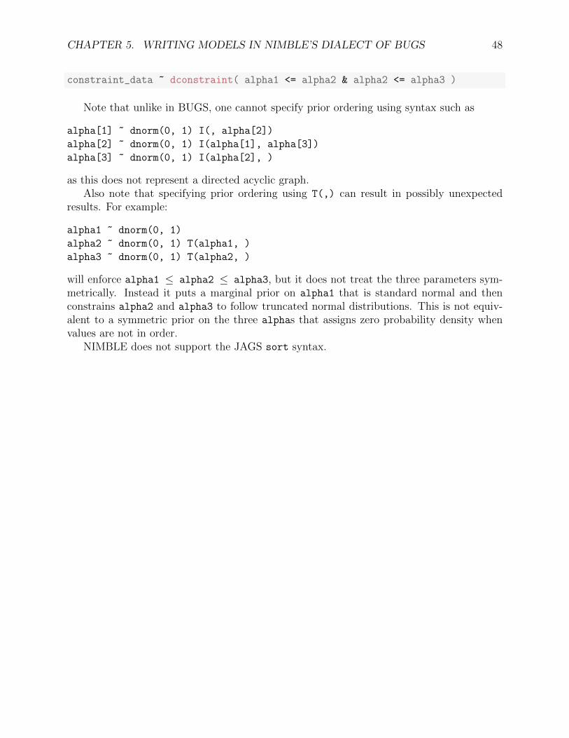
CHAPTER 5. WRITING MODELS IN NIMBLE’S DIALECT OF BUGS 48
constraint_data ~ dconstraint( alpha1 <= alpha2 & alpha2 <= alpha3 )
Note that unlike in BUGS, one cannot specify prior ordering using syntax such as
alpha[1] ~ dnorm(0, 1) I(, alpha[2])
alpha[2] ~ dnorm(0, 1) I(alpha[1], alpha[3])
alpha[3] ~ dnorm(0, 1) I(alpha[2], )
as this does not represent a directed acyclic graph.Also note that specifying prior ordering using T(,) can result in possibly unexpected
results. For example:
alpha1 ~ dnorm(0, 1)
alpha2 ~ dnorm(0, 1) T(alpha1, )
alpha3 ~ dnorm(0, 1) T(alpha2, )
will enforce alpha1 ≤ alpha2 ≤ alpha3, but it does not treat the three parameters sym-metrically. Instead it puts a marginal prior on alpha1 that is standard normal and thenconstrains alpha2 and alpha3 to follow truncated normal distributions. This is not equiv-alent to a symmetric prior on the three alphas that assigns zero probability density whenvalues are not in order.
NIMBLE does not support the JAGS sort syntax.

Chapter 6
Building and using models
This chapter explains how to build and manipulate model objects starting from BUGS code.
6.1 Creating model objects
NIMBLE provides two functions for creating model objects: nimbleModel and readBUGSmodel.The first, nimbleModel, is more general and was illustrated in Chapter 2. The second,readBUGSmodel provides compatibility with BUGS file formats for models, variables, data,and initial values for MCMC.
In addition one can create new model objects from existing model objects.
6.1.1 Using nimbleModel to create a model
nimbleModel processes BUGS code to determine all the nodes, variables, and their relation-ships in a model. Any constants must be provided at this step. Data and initial values canoptionally be provided. BUGS code passed to nimbleModel must go through nimbleCode.
We look again at the pump example from the introduction:
pumpCode <- nimbleCode({for (i in 1:N){
theta[i] ~ dgamma(alpha,beta);
lambda[i] <- theta[i]*t[i];
x[i] ~ dpois(lambda[i])
}alpha ~ dexp(1.0);
beta ~ dgamma(0.1,1.0);
})
pumpConsts <- list(N = 10,
t = c(94.3, 15.7, 62.9, 126, 5.24,
31.4, 1.05, 1.05, 2.1, 10.5))
49

CHAPTER 6. BUILDING AND USING MODELS 50
pumpData <- list(x = c(5, 1, 5, 14, 3, 19, 1, 1, 4, 22))
pumpInits <- list(alpha = 1, beta = 1,
theta = rep(0.1, pumpConsts$N))
pump <- nimbleModel(code = pumpCode, name = "pump", constants = pumpConsts,
data = pumpData, inits = pumpInits)
Data and constants
NIMBLE makes a distinction between data and constants:
• Constants can never be changed and must be provided when a model is defined. Forexample, a vector of known index values, such as for block indices, helps define themodel graph itself and must be provided as constants. Variables used in the indexranges of for-loops must also be provided as constants.• Data is a label for the role a node plays in the model. Nodes marked as data will
by default be protected from any functions that would simulate over their values (seesimulate in Chapter 13), but it is possible to over-ride that default or to change theirvalues by direct assignment. This allows an algorithm to be applied to many data setsin the same model without re-creating the model each time. It also allows simulationof data in a model.
WinBUGS, OpenBUGS and JAGS do not allow data values to be changed or differentnodes to be labeled as data without starting from the beginning again. Hence they do notdistinguish between constants and data.
For compatibility with BUGS and JAGS, NIMBLE allows both to be provided in theconstants argument to nimbleModel, in which case NIMBLE handles values for stochasticnodes as data and everything else as constants.
Values for nodes that appear only on the right-hand side of BUGS declarations (e.g.,covariates/predictors) can be provided as constants or as data or initial values. There is noreal difference between providing as data or initial values and the values can be added afterbuilding a model via setInits or setData.
Providing data and initial values to an existing model
Whereas constants must be provided during the call to nimbleModel, data and initial valuescan be provided later via the model member functions setData and setInits. For example,if pumpData is a named list of data values (as above), then pump$setData(pumpData) setsthe named variables to the values in the list.
setData does two things: it sets the values of the data nodes, and it flags those nodesas containing data. nimbleFunction programmers can then use that information to controlwhether an algorithm should over-write data or not. For example, NIMBLE’s simulate
functions by default do not overwrite data values but can be told to do so. Values of datavariables can be replaced, and the indication of which nodes should be treated as data canbe reset by using the resetData method, e.g. pump$resetData().

CHAPTER 6. BUILDING AND USING MODELS 51
Missing data values
Sometimes one needs a model variable to have a mix of data and non-data, often due tomissing data values. In NIMBLE, when data values are provided, any nodes with NA valueswill not be labeled as data. A node following a multivariate distribution must be eitherentirely observed or entirely missing.
Here’s an example of running an MCMC on the pump model, with two of the observa-tions taken to be missing. Some of the steps in this example are documented more below.NIMBLE’s default MCMC configuration will treat the missing values as unknowns to besampled, as can be seen in the MCMC output here.
pumpMiss <- pump$newModel()
pumpMiss$resetData()
pumpDataNew <- pumpData
pumpDataNew$x[c(1, 3)] <- NA
pumpMiss$setData(pumpDataNew)
pumpMissConf <- configureMCMC(pumpMiss)
pumpMissConf$addMonitors('x', 'alpha', 'beta', 'theta')
## thin = 1: alpha, beta, x, theta
pumpMissMCMC <- buildMCMC(pumpMissConf)
Cobj <- compileNimble(pumpMiss, pumpMissMCMC)
niter <- 10
set.seed(0)
Cobj$pumpMissMCMC$run(niter)
## NULL
samples <- as.matrix(Cobj$pumpMissMCMC$mvSamples)
samples[1:5, 13:17]
## x[1] x[2] x[3] x[4] x[5]
## [1,] 17 1 2 14 3
## [2,] 11 1 4 14 3
## [3,] 14 1 9 14 3
## [4,] 11 1 24 14 3
## [5,] 9 1 29 14 3
Missing values may also occur in explanatory/predictor variables. Values for such vari-ables should be passed in via the data argument to nimbleModel, with NA for the missingvalues. In some contexts, one would want to specify distributions for such explanatoryvariables, for example so that an MCMC would impute the missing values.

CHAPTER 6. BUILDING AND USING MODELS 52
Defining alternative models with the same code
Avoiding code duplication is a basic principle of good programming. In NIMBLE, one canuse definition-time if-then-else statements to create different models from the same code. Asa simple example, say we have a linear regression model and want to consider including oromitting x[2] as an explanatory variable:
regressionCode <- nimbleCode({intercept ~ dnorm(0, sd = 1000)
slope1 ~ dnorm(0, sd = 1000)
if(includeX2) {slope2 ~ dnorm(0, sd = 1000)
for(i in 1:N)
predictedY[i] <- intercept + slope1 * x1[i] + slope2 * x2[i]
} else {for(i in 1:N) predictedY[i] <- intercept + slope1 * x1[i]
}sigmaY ~ dunif(0, 100)
for(i in 1:N) Y[i] ~ dnorm(predictedY[i], sigmaY)
})
includeX2 <- FALSE
modelWithoutX2 <- nimbleModel(regressionCode, constants = list(N = 30),
check=FALSE)
modelWithoutX2$getVarNames()
## [1] "intercept"
## [2] "slope1"
## [3] "predictedY"
## [4] "sigmaY"
## [5] "lifted_d1_over_sqrt_oPsigmaY_cP"
## [6] "Y"
## [7] "x1"
includeX2 <- TRUE
modelWithX2 <- nimbleModel(regressionCode, constants = list(N = 30),
check = FALSE)
modelWithX2$getVarNames()
## [1] "intercept"
## [2] "slope1"
## [3] "slope2"
## [4] "predictedY"
## [5] "sigmaY"
## [6] "lifted_d1_over_sqrt_oPsigmaY_cP"
## [7] "Y"
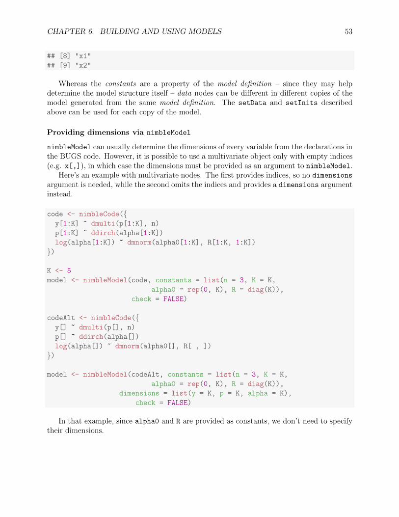
CHAPTER 6. BUILDING AND USING MODELS 53
## [8] "x1"
## [9] "x2"
Whereas the constants are a property of the model definition – since they may helpdetermine the model structure itself – data nodes can be different in different copies of themodel generated from the same model definition. The setData and setInits describedabove can be used for each copy of the model.
Providing dimensions via nimbleModel
nimbleModel can usually determine the dimensions of every variable from the declarations inthe BUGS code. However, it is possible to use a multivariate object only with empty indices(e.g. x[,]), in which case the dimensions must be provided as an argument to nimbleModel.
Here’s an example with multivariate nodes. The first provides indices, so no dimensions
argument is needed, while the second omits the indices and provides a dimensions argumentinstead.
code <- nimbleCode({y[1:K] ~ dmulti(p[1:K], n)
p[1:K] ~ ddirch(alpha[1:K])
log(alpha[1:K]) ~ dmnorm(alpha0[1:K], R[1:K, 1:K])
})
K <- 5
model <- nimbleModel(code, constants = list(n = 3, K = K,
alpha0 = rep(0, K), R = diag(K)),
check = FALSE)
codeAlt <- nimbleCode({y[] ~ dmulti(p[], n)
p[] ~ ddirch(alpha[])
log(alpha[]) ~ dmnorm(alpha0[], R[ , ])
})
model <- nimbleModel(codeAlt, constants = list(n = 3, K = K,
alpha0 = rep(0, K), R = diag(K)),
dimensions = list(y = K, p = K, alpha = K),
check = FALSE)
In that example, since alpha0 and R are provided as constants, we don’t need to specifytheir dimensions.

CHAPTER 6. BUILDING AND USING MODELS 54
6.1.2 Creating a model from standard BUGS and JAGS inputfiles
Users with BUGS and JAGS experience may have files set up in standard formats for use inBUGS and JAGS. readBUGSmodel can read in the model, data/constant values and initialvalues in those formats. It can also take information directly from R objects somewhatmore flexibly than nimbleModel, specifically allowing inputs set up similarly to those forBUGS and JAGS. In either case, after processing the inputs, it calls nimbleModel. Notethat unlike BUGS and JAGS, only a single set of initial values can be specified in creatinga model. Please see help(readBUGSmodel) for argument details.
As an example of using readBUGSmodel, let’s create a model for the pump example fromBUGS.
pumpDir <- system.file('classic-bugs', 'vol1', 'pump', package = 'nimble')
pumpModel <- readBUGSmodel('pump.bug', data = 'pump-data.R',
inits = 'pump-init.R', dir = pumpDir)
## Detected x as data within 'constants'.
Note that readBUGSmodel allows one to include var and data blocks in the model file asin some of the BUGS examples (such as inhaler). The data block pre-computes constantand data values. Also note that if data and inits are provided as files, the files shouldcontain R code that creates objects analogous to what would populate the list if a list wereprovided instead. Please see the JAGS manual examples or the classic bugs directory in theNIMBLE package for example syntax. NIMBLE by and large does not need the informationgiven in a var block but occasionally this is used to determine dimensionality, such as inthe case of syntax like xbar <- mean(x[]) where x is a variable that appears only on theright-hand side of BUGS expressions.
Note that NIMBLE does not handle formatting such as in some of the original BUGSexamples in which data was indicated with syntax such as data x in ‘x.txt’.
6.1.3 Making multiple instances from the same model definition
Sometimes it is useful to have more than one copy of the same model. For example, analgorithm (i.e., nimbleFunction) such as an MCMC will be bound to a particular modelbefore it is run. A user could build multiple algorithms to use the same model instance, orthey may want each algorithm to have its own instance of the model.
There are two ways to create new instances of a model, shown in this example:
simpleCode <- nimbleCode({for(i in 1:N) x[i] ~ dnorm(0, 1)
})
## Return the model definition only, not a built model
simpleModelDefinition <- nimbleModel(simpleCode, constants = list(N = 10),

CHAPTER 6. BUILDING AND USING MODELS 55
returnDef = TRUE, check = FALSE)
## Make one instance of the model
simpleModelCopy1 <- simpleModelDefinition$newModel(check = FALSE)
## Make another instance from the same definition
simpleModelCopy2 <- simpleModelDefinition$newModel(check = FALSE)
## Ask simpleModelCopy2 for another copy of itself
simpleModelCopy3 <- simpleModelCopy2$newModel(check = FALSE)
Each copy of the model can have different nodes flagged as data and different values inany nodes. They cannot have different values of N because that is a constant; it must be aconstant because it helps define the model.
6.2 NIMBLE models are objects you can query and
manipulate
NIMBLE models are objects that can be modified and manipulated from R. In this sectionwe introduce some basic ways to use a model object. Chapter 13 covers more topics forwriting algorithms that use models.
6.2.1 What are variables and nodes?
This section discusses some basic concepts and terminology to be able to speak about NIM-BLE models clearly.
Suppose we have created a model from the following BUGS code.
mc <- nimbleCode({a ~ dnorm(0, 0.001)
for(i in 1:5) {y[i] ~ dnorm(a, sd = 0.1)
for(j in 1:3)
z[i,j] ~ dnorm(y[i], tau)
}tau ~ dunif(0, 20)
y.squared[1:5] <- y[1:5]^2
})
model <- nimbleModel(mc, data = list(z = matrix(rnorm(15), nrow = 5)))
In NIMBLE terminology:
• The variables of this model are a, y, z, and y.squared.• The nodes of this model are a, y[1] , . . . , y[5], z[1,1] , . . . , z[5, 3], and y.squared[1:5].
In graph terminology, nodes are vertices in the model graph.

CHAPTER 6. BUILDING AND USING MODELS 56
• the node functions of this model are a ~ dnorm(0, 0.001), y[i] ~ dnorm(a, 0.1),z[i,j] ~ dnorm(y[i], sd = 0.1), and y.squared[1:5] <- y[1:5]^2. Each node’scalculations are handled by a node function. Sometimes the distinction between nodesand node functions is important, but when it is not important we may refer to bothsimply as nodes.• The scalar elements of this model include all the scalar nodes as well as the scalar
elements y.squared[1] , . . . , y.squared[5] of the multivariate node y.squared[1:5].
6.2.2 Determining the nodes and variables in a model
One can determine the variables in a model using getVarNames and the nodes in a modelusing getNodeNames. Optional arguments to getNodeNames allow you to select only certaintypes of nodes, as discussed in Section 13.1.1 and in the R help for getNodeNames.
model$getVarNames()
## [1] "a" "y"
## [3] "lifted_d1_over_sqrt_oPtau_cP" "z"
## [5] "tau" "y.squared"
model$getNodeNames()
## [1] "a"
## [2] "tau"
## [3] "y[1]"
## [4] "y[2]"
## [5] "y[3]"
## [6] "y[4]"
## [7] "y[5]"
## [8] "lifted_d1_over_sqrt_oPtau_cP"
## [9] "y.squared[1:5]"
## [10] "z[1, 1]"
## [11] "z[1, 2]"
## [12] "z[1, 3]"
## [13] "z[2, 1]"
## [14] "z[2, 2]"
## [15] "z[2, 3]"
## [16] "z[3, 1]"
## [17] "z[3, 2]"
## [18] "z[3, 3]"
## [19] "z[4, 1]"
## [20] "z[4, 2]"
## [21] "z[4, 3]"
## [22] "z[5, 1]"
## [23] "z[5, 2]"
## [24] "z[5, 3]"

CHAPTER 6. BUILDING AND USING MODELS 57
Note that some of the nodes may be “lifted” nodes introduced by NIMBLE (Section13.1.2). In this case lifted d1 over sqrt oPtau cP (this is a node for the standard devia-tion of the z nodes using NIMBLE’s canonical parameterization of the normal distribution)is the only lifted node in the model.
To determine the dependencies of one or more nodes in the model, you can use getDependenciesas discussed in Section 13.1.3.
6.2.3 Accessing nodes
Model variables can be accessed and set just as in R using $ and [[ ]]. For example
model$a <- 5
model$a
## [1] 5
model[["a"]]
## [1] 5
model$y[2:4] <- rnorm(3)
model$y
## [1] NA -0.9261095 -0.1771040 0.4020118 NA
model[["y"]][c(1, 5)] <- rnorm(2)
model$y
## [1] -0.7317482 -0.9261095 -0.1771040 0.4020118 0.8303732
model$z[1,]
## [1] -0.3340008 1.2079084 0.5210227
While nodes that are part of a variable can be accessed as above, each node also has itsown name that can be used to access it directly. For example, y[2] has the name “y[2]” andcan be accessed by that name as follows:
model[["y[2]"]]
## [1] -0.9261095
model[["y[2]"]] <- -5
model$y
## [1] -0.7317482 -5.0000000 -0.1771040 0.4020118 0.8303732
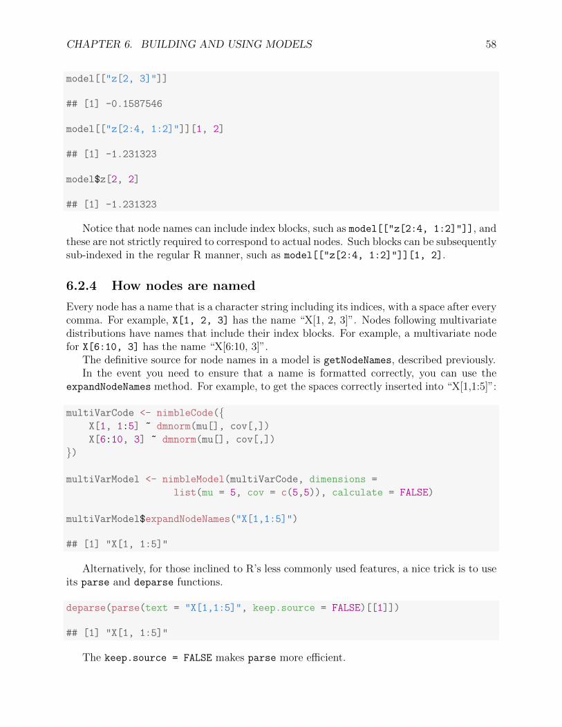
CHAPTER 6. BUILDING AND USING MODELS 58
model[["z[2, 3]"]]
## [1] -0.1587546
model[["z[2:4, 1:2]"]][1, 2]
## [1] -1.231323
model$z[2, 2]
## [1] -1.231323
Notice that node names can include index blocks, such as model[["z[2:4, 1:2]"]], andthese are not strictly required to correspond to actual nodes. Such blocks can be subsequentlysub-indexed in the regular R manner, such as model[["z[2:4, 1:2]"]][1, 2].
6.2.4 How nodes are named
Every node has a name that is a character string including its indices, with a space after everycomma. For example, X[1, 2, 3] has the name “X[1, 2, 3]”. Nodes following multivariatedistributions have names that include their index blocks. For example, a multivariate nodefor X[6:10, 3] has the name “X[6:10, 3]”.
The definitive source for node names in a model is getNodeNames, described previously.In the event you need to ensure that a name is formatted correctly, you can use the
expandNodeNames method. For example, to get the spaces correctly inserted into “X[1,1:5]”:
multiVarCode <- nimbleCode({X[1, 1:5] ~ dmnorm(mu[], cov[,])
X[6:10, 3] ~ dmnorm(mu[], cov[,])
})
multiVarModel <- nimbleModel(multiVarCode, dimensions =
list(mu = 5, cov = c(5,5)), calculate = FALSE)
multiVarModel$expandNodeNames("X[1,1:5]")
## [1] "X[1, 1:5]"
Alternatively, for those inclined to R’s less commonly used features, a nice trick is to useits parse and deparse functions.
deparse(parse(text = "X[1,1:5]", keep.source = FALSE)[[1]])
## [1] "X[1, 1:5]"
The keep.source = FALSE makes parse more efficient.

CHAPTER 6. BUILDING AND USING MODELS 59
6.2.5 Why use node names?
Syntax like model[["z[2, 3]"]] may seem strange at first, because the natural habit of anR user would be model[["z"]][2,3]. To see its utility, consider the example of writing thenimbleFunction given in Section 2.8. By giving every scalar node a name, even if it is part ofa multivariate variable, one can write functions in R or NIMBLE that access any single nodeby a name, regardless of the dimensionality of the variable in which it is embedded. This isparticularly useful for NIMBLE, which resolves how to access a particular node during thecompilation process.
6.2.6 Checking if a node holds data
Finally, you can query whether a node is flagged as data using the isData method appliedto one or more nodes or nodes within variables:
model$isData('z[1]')
## [1] TRUE
model$isData(c('z[1]', 'z[2]', 'a'))
## [1] TRUE TRUE FALSE
model$isData('z')
## [1] TRUE TRUE TRUE TRUE TRUE TRUE TRUE TRUE TRUE TRUE TRUE TRUE
## [13] TRUE TRUE TRUE
model$isData('z[1:3, 1]')
## [1] TRUE TRUE TRUE

Part III
Algorithms in NIMBLE
60

Chapter 7
MCMC
NIMBLE provides a variety of paths to creating and executing an MCMC algorithm, whichdiffer greatly in their simplicity of use, and also in the options available and customizability.
The most direct approach to invoking the MCMC engine is using the nimbleMCMC func-tion (Section 7.1). This one-line call creates and executes an MCMC, and provides a widerange of options for controlling the MCMC: specifying monitors, burn-in, and thinning, run-ning multiple MCMC chains with different initial values, and returning posterior samples,summary statistics, and/or a WAIC value. However, this approach is restricted to usingNIMBLE’s default MCMC algorithm; further customization of, for example, the specificsamplers employed, is not possible.
The lengthier and more customizable approach to invoking the MCMC engine on aparticular NIMBLE model object involves the following steps:
1. (Optional) Create and customize an MCMC configuration for a particular model:
(a) Use configureMCMC to create an MCMC configuration (see Section 7.2). Theconfiguration contains a list of samplers with the node(s) they will sample.
(b) (Optional) Customize the MCMC configuration:
i. Add, remove, or re-order the list of samplers (Section 7.9 and help(samplers)
in R for details), including adding your own samplers (Section 15.5);ii. Change the tuning parameters or adaptive properties of individual samplers;iii. Change the variables to monitor (record for output) and thinning intervals
for MCMC samples.
2. Use buildMCMC to build the MCMC object and its samplers either from the model (us-ing default MCMC configuration) or from a customized MCMC configuration (Section7.3).
3. Compile the MCMC object (and the model), unless one is debugging and wishes torun the uncompiled MCMC.
4. Run the MCMC and extract the samples (Sections 7.4, 7.5 and 7.6).5. Optionally, calculate the WAIC using the posterior samples (Section 7.7).
NIMBLE provides two additional functions which facilitate the comparison of multiple,different, MCMC algorithms:
61

CHAPTER 7. MCMC 62
• MCMCsuite can run multiple, different MCMCs for the same model. These can includemultiple NIMBLE MCMCs from different configurations as well as external MCMCssuch as from WinBUGS, OpenBUGS, JAGS or Stan (Section 7.11).• compareMCMCs manages multiple calls to MCMCsuite and generates html pages com-
paring performance of different MCMCs.
End-to-end examples of MCMC in NIMBLE can be found in Sections 2.5-2.6 and Section7.10.
7.1 One-line invocation of MCMC: nimbleMCMC
The most direct approach to executing an MCMC algorithm in NIMBLE is using nimbleMCMC.This single function can be used to create an underlying model and associated MCMC algo-rithm, compile both of these, execute the MCMC, and return samples, summary statistics,and a WAIC value. This approach circumvents the longer (and more flexible) approachusing nimbleModel, configureMCMC, buildMCMC, compileNimble, and runMCMC, which isdescribed subsequently.
The nimbleMCMC function provides control over the:
• number of MCMC iterations in each chain;• number of MCMC chains to execute;• number of burn-in samples to discard from each chain;• thinning interval on which samples should be recorded;• model variables to monitor and return posterior samples;• initial values, or a function for generating initial values for each chain;• setting the random number seed;• returning posterior samples as a matrix or a coda mcmc object;• returning posterior summary statistics; and• returning a WAIC value calculated using samples from all chains.
This entry point for using nimbleMCMC is the code, constants, data, and inits argu-ments that are used for building a NIMBLE model (see Chapters 5 and 6). However, whenusing nimbleMCMC, the inits argument can also specify a list of lists of initial values thatwill be used for each MCMC chain, or a function that generates a list of initial values, whichwill be generated at the onset of each chain. As an alternative entry point, a NIMBLE model
object can also be supplied to nimbleMCMC, in which case this model will be used to buildthe MCMC algorithm.
Based on its arguments, nimbleMCMC optionally returns any combination of
• Posterior samples,• Posterior summary statistics, and• WAIC value.
The above are calculated and returned for each MCMC chain. Additionally, posteriorsummary statistics are calculated for all chains combined when multiple chains are run.
Several example usages of nimbleMCMC are shown below:

CHAPTER 7. MCMC 63
code <- nimbleCode({mu ~ dnorm(0, sd = 1000)
sigma ~ dunif(0, 1000)
for(i in 1:10)
x[i] ~ dnorm(mu, sd = sigma)
})data <- list(x = c(2, 5, 3, 4, 1, 0, 1, 3, 5, 3))
initsFunction <- function() list(mu = rnorm(1,0,1), sigma = runif(1,0,10))
## execute one MCMC chain, monitoring the "mu" and "sigma" variables,
## with thinning interval 10. fix the random number seed for reproducible
## results. by default, only returns posterior samples.
mcmc.out <- nimbleMCMC(code = code, data = data, inits = initsFunction,
monitors = c("mu", "sigma"), thin = 10,
niter = 20000, nchains = 1, setSeed = TRUE)
## note that the inits argument to nimbleModel must be a list of
## initial values, whereas nimbleMCMC can accept inits as a function
## for generating new initial values for each chain.
initsList <- initsFunction()
Rmodel <- nimbleModel(code, data = data, inits = initsList)
## using the existing Rmodel object, execute three MCMC chains with
## specified burn-in. return samples, summary statistics, and WAIC.
mcmc.out <- nimbleMCMC(model = Rmodel,
niter = 20000, nchains = 3, nburnin = 2000,
summary = TRUE, WAIC = TRUE)
## run ten chains, generating random initial values for each
## chain using the inits function specified above.
## only return summary statistics from each chain; not all the samples.
mcmc.out <- nimbleMCMC(model = Rmodel, nchains = 10, inits = initsFunction,
samples = FALSE, summary = TRUE)
See help(nimbleMCMC) for further details.
7.2 The MCMC configuration
The MCMC configuration contains information needed for building an MCMC. When nocustomization is needed, one can jump directly to the buildMCMC step below. An MCMCconfiguration is an object of class MCMCconf, which includes:
• The model on which the MCMC will operate• The model nodes which will be sampled (updated) by the MCMC

CHAPTER 7. MCMC 64
• The samplers and their internal configurations, called control parameters• Two sets of variables that will be monitored (recorded) during execution of the MCMC
and thinning intervals for how often each set will be recorded. Two sets are allowedbecause it can be useful to monitor different variables at different intervals
7.2.1 Default MCMC configuration
Assuming we have a model named Rmodel, the following will generate a default MCMCconfiguration:
mcmcConf <- configureMCMC(Rmodel)
The default configuration will contain a single sampler for each node in the model, andthe default ordering follows the topological ordering of the model.
Default assignment of sampler algorithms
The default sampler assigned to a stochastic node is determined by the following, in orderof precedence:
1. If the node has no stochastic dependents, a posterior predictive sampler is assigned.This sampler sets the new value for the node simply by simulating from its distribution.
2. If the node has a conjugate relationship between its prior distribution and the distri-butions of its stochastic dependents, a conjugate (‘Gibbs’) sampler is assigned.
3. If the node follows a multinomial distribution, then a RW multinomial sampler isassigned. This is a discrete random-walk sampler in the space of multinomial outcomes.
4. If a node follows a Dirichlet distribution, then a RW dirichlet sampler is assigned.This is a random walk sampler in the space of the simplex defined by the Dirichlet.
5. If the node follows any other multivariate distribution, then a RW block sampler isassigned for all elements. This is a Metropolis-Hastings adaptive random-walk samplerwith a multivariate normal proposal [16].
6. If the node is binary-valued (strictly taking values 0 or 1), then a binary sampler isassigned. This sampler calculates the conditional probability for both possible nodevalues and draws the new node value from the conditional distribution, in effect makinga Gibbs sampler.
7. If the node is otherwise discrete-valued, then a slice sampler is assigned [14].8. If none of the above criteria are satisfied, then a RW sampler is assigned. This is a
Metropolis-Hastings adaptive random-walk sampler with a univariate normal proposaldistribution.
These sampler assignment rules can be inspected, reordered, and easily modified using thesystem option nimbleOptions("MCMCdefaultSamplerAssignmentRules"), and customizedsamplerAssignmentRules objects.
Details of each sampler and its control parameters can be found by invoking help(samplers)
in R with nimble loaded.

CHAPTER 7. MCMC 65
Sampler assignment rules
The behavior of configureMCMC can be customized to control how samplers are assigned.A new set of sampler assignment rules can be created using samplerAssignmentRules,which can be modified using the addRule and reorder methods, then passed as an ar-gument to configureMCMC. Alternatively, the default behavior of configureMCMC can bealtered by setting the system option MCMCdefaultSamplerAssignmentRules to a customsamplerAssignmentRules object. See help(samplerAssignmentRules) for details.
Options to control default sampler assignments
As a lightweight alternative to using samplerAssignmentRules, very basic control of defaultsampler assignments is provided via two arguments to configureMCMC. The useConjugacy
argument controls whether conjugate samplers are assigned when possible, and themultivariateNodesAsScalars argument controls whether scalar elements of multivariatenodes are sampled individually. See help(configureMCMC) for usage details.
Default monitors
The default MCMC configuration includes monitors on all top-level stochastic nodes of themodel. Only variables that are monitored will have their samples saved for use outside ofthe MCMC. MCMC configurations include two sets of monitors, each with different thinningintervals. By default, the second set of monitors (monitors2) is empty.
Automated parameter blocking
The default configuration may be replaced by one generated from an automated parameterblocking algorithm. This algorithm determines groupings of model nodes that, when jointlysampled with a RW block sampler, increase overall MCMC efficiency. Overall efficiency isdefined as the effective sample size of the slowest-mixing node divided by computation time.This is done by:
autoBlockConf <- configureMCMC(Rmodel, autoBlock = TRUE)
Note that this using autoBlock = TRUE compiles and runs MCMCs, progressively ex-ploring different sampler assignments, so it takes some time and generates some output.It is most useful for determining effective blocking strategies that can be re-used for laterruns. The additional control argument autoIt may also be provided to indicate the numberof MCMC samples to be used in each trial of the automated blocking procedure (default20,000).
7.2.2 Customizing the MCMC configuration
The MCMC configuration may be customized in a variety of ways, either through additionalnamed arguments to configureMCMC or by calling methods of an existing MCMCconf object.

CHAPTER 7. MCMC 66
Controlling which nodes to sample
One can create an MCMC configuration with default samplers on just a particular set ofnodes using the nodes argument to configureMCMC. The value for the nodes argument maybe a character vector containing node and/or variable names. In the case of a variable name,a default sampler will be added for all stochastic nodes in the variable. The order of samplerswill match the order of nodes. Any deterministic nodes will be ignored.
If a data node is included in nodes, it will be assigned a sampler. This is the only way inwhich a default sampler may be placed on a data node and will result in overwriting datavalues in the node.
Creating an empty configuration
If you plan to customize the choice of all samplers, it can be useful to obtain a configurationwith no sampler assignments at all. This can be done by any of nodes = NULL, nodes =
character(), or nodes = list().
Overriding the default sampler assignment rules
The default rules used for assigning samplers to model nodes can be overridden using therules argument to configureMCMC. This argument must be an object of classsamplerAssignmentRules, which defines an ordered set of rules for assigning samplers.Rules can be modified and reordered, to give different precedence to particular samplers, orto assign user-defined samplers (see section 15.5). The following example creates a new setof rules (which initially contains the default assignment rules), reorders the rules, adds anew rule, then uses these rules to create an MCMC configuration object.
my_rules <- samplerAssignmentRules()
my_rules$reorder(c(8, 1:7))
my_rules$addRule(condition = quote(model$getDistribution(node) == "dmnorm"),
sampler = new_dmnorm_sampler)
mcmcConf <- configureMCMC(Rmodel, rules = my_rules)
In addition, the default behavior of configureMCMC can be altered by setting the systemoption nimbleOptions(MCMCdefaultSamplerAssignmentRules = my rules), or reset tothe original default behavior using nimbleOptions(MCMCdefaultSamplerAssignmentRules
= samplerAssignmentRules()).
Overriding the default sampler control list values
The default values of control list elements for all sampling algorithms may be overriddenthrough use of the control argument to configureMCMC, which should be a named list.Named elements in the control argument will be used for all default samplers and anysubsequent sampler added via addSampler (see below). For example, the following willcreate the default MCMC configuration, except all RW samplers will have their initial scaleset to 3, and none of the samplers (RW, or otherwise) will be adaptive.

CHAPTER 7. MCMC 67
mcmcConf <- configureMCMC(Rmodel, control = list(scale = 3, adaptive = FALSE))
When adding samplers to a configuration using addSampler, the default control list canalso be over-ridden.
Adding samplers to the configuration: addSampler
Samplers may be added to a configuration using the addSampler method of the MCMCconf
object. The first argument gives the node(s) to be sampled, called the target, as a charactervector. The second argument gives the type of sampler, which may be provided as a characterstring or a nimbleFunction object. Valid character strings are indicated in help(samplers)
(do not include "sampler "). Added samplers can be labeled with a name argument, whichis used in output of printSamplers.
Writing a new sampler as a nimbleFunction is covered in Section 15.5.The hierarchy of precedence for control list elements for samplers is:
1. The control list argument to addSampler;2. The control list argument to configureMCMC;3. The default values, as defined in the sampling algorithm setup function.
Samplers added by addSampler will be appended to the end of current sampler list.Adding a sampler for a node will not automatically remove any existing samplers on thatnode.
Printing, re-ordering, modifying and removing samplers: printSamplers,getSamplerDefinition, and removeSamplers
The current, ordered, list of all samplers in the MCMC configuration may be printed bycalling the printSamplers method. When you want to see only samplers acting on specificmodel nodes or variables, provide those names as an argument to printSamplers. TheprintSamplers method accepts arguments controlling the level of detail displayed as dis-cussed in its R help information.
The nimbleFunction definition underlying a particular sampler may be viewed using thegetSamplerDefinition method, using the sampler index as an argument. A node nameargument may also be supplied, in which case the definition of the first sampler acting onthat node is returned. In all cases, getSamplerDefinition only returns the definition ofthe first sampler specified either by index or node name.
## Return the definition of the third sampler in the mcmcConf object
mcmcConf$getSamplerDefinition(3)
## Return the definition of the first sampler acting on node "x",
## or the first of any indexed nodes comprising the variable "x"
mcmcConf$getSamplerDefinition("x")

CHAPTER 7. MCMC 68
The existing samplers may be re-ordered using the setSamplers method. The ind argu-ment is a vector of sampler indices, or a character vector of model node or variable names.Here are a few examples. Each example assumes the MCMCconf object initially contains 10samplers, and each example is independent of the others.
## Truncate the current list of samplers to the first 5
mcmcConf$setSamplers(ind = 1:5)
## Retain only the third sampler, which will subsequently
## become the first sampler
mcmcConf$setSamplers(ind = 3)
## Reverse the ordering of the samplers
mcmcConf$setSamplers(ind = 10:1)
## The new set of samplers becomes the
## {first, first, first, second, third} from the current list.
## Upon each iteration of the MCMC, the 'first' sampler will
## be executed 3 times, however each instance of the sampler
## will be independent in terms of scale, adaptation, etc.
mcmcConf$setSamplers(ind = c(1, 1, 1, 2, 3))
## Set the list of samplers to only those acting on model node "alpha"
mcmcConf$setSamplers("alpha")
## Set the list of samplers to those acting on any components of the
## model variables "x", "y", or "z".
mcmcConf$setSamplers(c("x", "y", "z"))
Samplers may be removed from the current sampler ordering with the removeSamplers
method. The following examples again assume that mcmcConf initially contains 10 samplers,and each example is independent of the others. removeSamplers accepts a vector of numericindices of samplers to be removed or a character vector. In the latter case, all samplers actingon the named target model nodes will be removed.
## Remove the first sampler
mcmcConf$removeSamplers(ind = 1)
## Remove the last five samplers
mcmcConf$removeSamplers(ind = 6:10)
## Remove all samplers,
## resulting in an empty MCMC configuration, containing no samplers
mcmcConf$removeSamplers(ind = 1:10)

CHAPTER 7. MCMC 69
## Remove all samplers acting on "x" or any component of it
mcmcConf$removeSamplers("x")
## Default: providing no argument removes all samplers
mcmcConf$removeSamplers()
Customizing individual sampler configurations: getSamplers, setSamplers, setName,setSamplerFunction, setTarget, and setControl
Each sampler in an MCMCconf object is represented by a sampler configuration as a samplerConfobject. Each samplerConf is a reference class object containing the following (required)fields: name (a character string), samplerFunction (a valid nimbleFunction sampler), target(the model node to be sampled), and control (list of control arguments). The MCMCconf
method getSamplers allows access to the samplerConf objects. These can be modifiedand then passed as an argument to setSamplers to over-write the current list of samplersin the MCMC configuration object. However, no checking of the validity of this modifiedlist is performed; if the list of samplerConf objects is corrupted to be invalid, incorrectbehavior will result at the time of calling buildMCMC. The fields of a samplerConf objectcan be modified using the access functions setName(name), setSamplerFunction(fun),setTarget(target, model), and setControl(control).
Here are some examples:
## retrieve samplerConf list
samplerConfList <- mcmcConf$getSamplers()
## change the name of the first sampler
samplerConfList[[1]]$setName("newNameForThisSampler")
## change the sampler function of the second sampler,
## assuming existance of a nimbleFunction 'anotherSamplerNF',
## which represents a valid nimbleFunction sampler.
samplerConfList[[2]]$setSamplerFunction(anotherSamplerNF)
## change the 'adaptive' element of the control list of the third sampler
control <- samplerConfList[[3]]$control
control$adaptive <- FALSE
samplerConfList[[3]]$setControl(control)
## change the target node of the fourth sampler
samplerConfList[[4]]$setTarget("y", model) ## model argument required
## use this modified list of samplerConf objects in the MCMC configuration
mcmcConf$setSamplers(samplerConfList)

CHAPTER 7. MCMC 70
Customizing the sampler execution order
The ordering of sampler execution can be controlled as well. This allows for sampler functionsto execute multiple times within a single MCMC iteration, or the execution of differentsampler functions to be interleaved with one another.
The sampler execution order is set using the function setSamplerExecutionOrder, andthe current ordering of execution is retrieved using getSamplerExecutionOrder. For exam-ple, assuming the MCMC configuration object mcmcConf contains 5 samplers:
## first sampler to execute twice, in succession:
mcmcConf$setSamplerExecutionOrder(c(1, 1, 2, 3, 4, 5))
## first sampler to execute multiple times, interleaved:
mcmcConf$setSamplerExecutionOrder(c(1, 2, 1, 3, 1, 4, 1, 5))
## fourth sampler to execute 10 times, only
mcmcConf$setSamplerExecutionOrder(rep(4, 10))
## omitting the argument to setSamplerExecutionOrder()
## resets the ordering to each sampler executing once, sequentially
mcmcConf$setSamplerExecutionOrder()
## retrieve the current ordering of sampler execution
ordering <- mcmcConf$getSamplerExecutionOrder()
## print the sampler functions in the order of execution
mcmcConf$printSamplers(executionOrder = TRUE)
Monitors and thinning intervals: printMonitors, getMonitors, addMonitors, setThin,and resetMonitors
An MCMC configuration object contains two independent sets of variables to monitor, eachwith their own thinning interval: thin corresponding to monitors, and thin2 correspondingto monitors2. Monitors operate at the variable level. Only entire model variables may bemonitored. Specifying a monitor on a node, e.g., x[1], will result in the entire variable x
being monitored.The variables specified in monitors and monitors2 will be recorded (with thinning in-
terval thin) into objects called mvSamples and mvSamples2, contained within the MCMCobject. These are both modelValues objects; modelValues are NIMBLE data structures usedto store multiple sets of values of model variables1. These can be accessed as the member datamvSamples and mvSamples2 of the MCMC object, and they can be converted to matricesusing as.matrix (see Section 7.6).
Monitors may be added to the MCMC configuration either in the original call to configureMCMCor using the addMonitors method:
1See Section 14.1 for general information on modelValues.

CHAPTER 7. MCMC 71
## Using an argument to configureMCMC
mcmcConf <- configureMCMC(Rmodel, monitors = c("alpha", "beta"),
monitors2 = "x")
## Calling a member method of the mcmcconf object
## This results in the same monitors as above
mcmcConf$addMonitors("alpha", "beta")
mcmcConf$addMonitors2("x")
Similarly, either thinning interval may be set at either step:
## Using an argument to configureMCMC
mcmcConf <- configureMCMC(Rmodel, thin = 1, thin2 = 100)
## Calling a member method of the mcmcConf object
## This results in the same thinning intervals as above
mcmcConf$setThin(1)
mcmcConf$setThin2(100)
The current lists of monitors and thinning intervals may be displayed using the printMonitorsmethod. Both sets of monitors (monitors and monitors2) may be reset to empty charactervectors by calling the resetMonitors method. The methods getMonitors and getMonitors2
return the currently specified monitors and monitors2 as character vectors.
Monitoring model log-probabilities
To record model log-probabilities from an MCMC, one can add monitors for logProb variables(which begin with the prefix logProb ) that correspond to variables with (any) stochasticnodes. For example, to record and extract log-probabilities for the variables alpha, sigma mu,and Y:
mcmcConf <- configureMCMC(Rmodel)
mcmcConf$addMonitors("logProb_alpha", "logProb_sigma_mu", "logProb_Y")
Rmcmc <- buildMCMC(mcmcConf)
Cmodel <- compileNimble(Rmodel)
Cmcmc <- compileNimble(Rmcmc, project = Rmodel)
Cmcmc$run(10000)
samples <- as.matrix(Cmcmc$mvSamples)
The samples matrix will contain both MCMC samples and model log-probabilities.
7.3 Building and compiling the MCMC
Once the MCMC configuration object has been created, and customized to one’s liking, itmay be used to build an MCMC function:

CHAPTER 7. MCMC 72
Rmcmc <- buildMCMC(mcmcConf, enableWAIC = TRUE)
buildMCMC is a nimbleFunction. The returned object Rmcmc is an instance of the nimble-Function specific to configuration mcmcConf (and of course its associated model).
Note that if you would like to be able to calculate the WAIC of the model after theMCMC function has been run, you must set enableWAIC = TRUE as an argument to eitherconfigureMCMC or buildMCMC, or set nimbleOptions(enableWAIC = TRUE), which will en-able WAIC calculations for all subsequently built MCMC functions. For more informationon WAIC calculations, see Section 7.7 or help(buildMCMC) in R.
When no customization is needed, one can skip configureMCMC and simply provide amodel object to buildMCMC. The following two MCMC functions will be identical:
mcmcConf <- configureMCMC(Rmodel) ## default MCMC configuration
Rmcmc1 <- buildMCMC(mcmcConf)
Rmcmc2 <- buildMCMC(Rmodel) ## uses the default configuration for Rmodel
For speed of execution, we usually want to compile the MCMC function to C++ (as isthe case for other NIMBLE functions). To do so, we use compileNimble. If the model hasalready been compiled, it should be provided as the project argument so the MCMC willbe part of the same compiled project. A typical compilation call looks like:
Cmcmc <- compileNimble(Rmcmc, project = Rmodel)
Alternatively, if the model has not already been compiled, they can be compiled togetherin one line:
Cmcmc <- compileNimble(Rmodel, Rmcmc)
Note that if you compile the MCMC with another object (the model in this case), you’llneed to explicitly refer to the MCMC component of the resulting object to be able to runthe MCMC:
Cmcmc$Rmcmc$run(niter = 1000)
7.4 User-friendly execution of MCMC algorithms: runMCMC
Once an MCMC algorithm has been created using buildMCMC, the function runMCMC canbe used to run multiple chains and extract posterior samples, summary statistics and/or aWAIC value. This is a simpler approach to executing an MCMC algorithm, than the processof executing and extracting samples as described in Sections 7.5 and 7.6.
runMCMC also provides several user-friendly options such as burn-in, thinning, runningmultiple chains, and different initial values for each chain. However, using runMCMC does not

CHAPTER 7. MCMC 73
support several lower-level options, such as timing the individual samplers internal to theMCMC, continuing an exisiting MCMC run (picking up where it left off), or modifying thesampler execution ordering.
runMCMC takes arguments that will control the following aspects of the MCMC:
• Number of iterations in each chain;• Number of chains;• Number of burn-in samples to discard from each chain;• Thinning interval for recording samples;• Initial values, or a function for generating initial values for each chain;• Setting the random number seed;• Returning the posterior samples as a coda mcmc object;• Returning summary statistics calculated from each chains; and• Returning a WAIC value calculated using samples from all chains.
The following examples demonstrate some uses of runMCMC, and assume the existence ofCmcmc, a compiled MCMC algorithm.
## run a single chain, and return a matrix of samples
mcmc.out <- runMCMC(Cmcmc)
## run three chains of 10000 samples, discard initial burnin of 1000,
## record samples thereafter using a thinning interval of 10,
## and return of list of sample matrices
mcmc.out <- runMCMC(Cmcmc, niter=10000, nburnin=1000, thin=10, nchains=3)
## run three chains, returning posterior samples, summary statistics,
## and the WAIC value for each chain
mcmc.out <- runMCMC(Cmcmc, nchains = 3, summary = TRUE, WAIC = TRUE)
## run two chains, and specify the initial values for each
initsList <- list(list(mu = 1, sigma = 1),
list(mu = 2, sigma = 10))
mcmc.out <- runMCMC(Cmcmc, nchains = 2, inits = initsList)
## run ten chains of 100,000 iterations each, using a function to
## generate initial values and a fixed random number seed for each chain.
## only return summary statistics from each chain; not all the samples.
initsFunction <- function()
list(mu = rnorm(1,0,1), sigma = runif(1,0,100))
mcmc.out <- runMCMC(Cmcmc, niter = 100000, nchains = 10,
inits = initsFunction, setSeed = TRUE,
samples = FALSE, summary = TRUE)
See help(runMCMC) for further details.

CHAPTER 7. MCMC 74
7.5 Running the MCMC
The MCMC algorithm (either the compiled or uncompiled version) can be executed using themember method mcmc$run (see help(buildMCMC) in R). The run method has one requiredargument, niter, the number of iterations to be run.
The run method has optional arguments thin and thin2. These can be used to specifythinning intervals for recording samples (corresponding to monitors and monitors2). Ifeither of these arguments are provided, they will override the thinning intervals that werespecified in the original MCMC configuration object.
The run method has an optional reset argument. When reset = TRUE (the defaultvalue), the following occurs prior to running the MCMC:
• All model nodes are checked and filled or updated as needed, in valid (topological)order. If a stochastic node is missing a value, it is populated using a call to simulate
and its log probability value is calculated. The values of deterministic nodes are cal-culated from their parent nodes. If any right-hand-side-only nodes (e.g., explanatoryvariables) are missing a value, an error results.• All MCMC sampler functions are reset to their initial state: the initial values of any
sampler control parameters (e.g., scale, sliceWidth, or propCov) are reset to theirinitial values, as were specified by the original MCMC configuration.• The internal modelValues objects mvSamples and mvSamples2 are each resized to the
appropriate length for holding the requested number of samples (niter/thin, andniter/thin2, respectively).
When mcmc$run(niter, reset = FALSE) is called, the MCMC picks up from where itleft off, continuing the previous chain and expanding the output as needed. No values in themodel are checked or altered, and sampler functions are not reset to their initial states.
The run method takes an optional simulateAll argument. When simulateAll = TRUE,the simulate method of all stochastic nodes is called before running the MCMC. Thisgenerates a new set of initial values. It should be used with caution since values drawn frompriors may be extreme or invalid in some models.
7.5.1 Measuring sampler computation times: getTimes
If you want to obtain the computation time spent in each sampler, you can set time=TRUE asa run-time argument and then use the method getTimes() obtain the times. For example,
Cmcmc$run(niter, time = TRUE)
Cmcmc$getTimes()
will return a vector of the total time spent in each sampler, measured in seconds.
7.6 Extracting MCMC samples
After executing the MCMC, the output samples can be extracted as follows:

CHAPTER 7. MCMC 75
mvSamples <- mcmc$mvSamples
mvSamples2 <- mcmc$mvSamples2
These modelValues objects can be converted into matrices using as.matrix:
samplesMatrix <- as.matrix(mvSamples)
samplesMatrix2 <- as.matrix(mvSamples2)
The column names of the matrices will be the node names of nodes in the monitoredvariables. Then, for example, the mean of the samples for node x[2] could be calculated as:
mean(samplesMatrix[, "x[2]"])
Obtaining samples as matrices is most common, but see Section 14.1 for more aboutprogramming with modelValues objects, especially if you want to write nimbleFunctions touse the samples.
7.7 Calculating WAIC
Once an MCMC algorithm has been run, as described in ??, the WAIC [19] can be calculatedfrom the posterior samples produced by the MCMC algorithm. Note that in order to calculatethe WAIC value after running an MCMC algorithm, the argument enableWAIC = TRUE musthave been supplied to configureMCMC or to buildMCMC, or the enableWAIC NIMBLE optionmust have been set to TRUE.
The WAIC is calculated by calling the member method mcmc$calculateWAIC (see help(buildMCMC)in R for more details). The calculateWAIC method has one required argument, nburnin,the number of initial samples to discard prior to WAIC calculation. nburnin defaults to 0.
Cmcmc$calculateWAIC(nburnin = 100)
7.8 k-fold cross-validation
The runCrossValidate function in NIMBLE performs k-fold cross-validation on a nimbleModelfit via MCMC. More information can be found by calling help(runCrossValidate).
7.9 Samplers provided with NIMBLE
Most documentation of MCMC samplers provided with NIMBLE can be found by invokinghelp(samplers) in R. Here we provide additional explanation of conjugate samplers and howcomplete customization can be achieved by making a sampler use an arbitrary log-likelihoodfunction, such as to build a particle MCMC algorithm.

CHAPTER 7. MCMC 76
7.9.1 Conjugate (‘Gibbs’) samplers
By default, configureMCMC() and buildMCMC() will assign conjugate samplers to all nodessatisfying a conjugate relationship, unless the option useConjugacy = FALSE is specified.
The current release of NIMBLE supports conjugate sampling of the relationships listedin Table 7.12.
Prior Distribution Sampling (Dependent Node) Distribution Parameter
Beta Bernoulli prob
Binomial prob
Negative Binomial prob
Dirichlet Multinomial prob
Categorical prob
Flat Normal mean
Lognormal meanlog
Gamma Poisson lambda
Normal tau
Lognormal taulog
Gamma rate
Inverse Gamma scale
Exponential rate
Weibull lambda
Halfflat Normal sd
Lognormal sdlog
Inverse Gamma Normal var
Lognormal varlog
Gamma scale
Inverse Gamma rate
Exponential scale
Normal Normal mean
Lognormal meanlog
Multivariate Normal Multivariate Normal mean
Wishart Multivariate Normal prec
Inverse Wishart Multivariate Normal cov
Table 7.1: Conjugate relationships supported by NIMBLE’s MCMC engine.
Conjugate sampler functions may (optionally) dynamically check that their own pos-terior likelihood calculations are correct. If incorrect, a warning is issued. However, thisfunctionality will roughly double the run-time required for conjugate sampling. By default,this option is disabled in NIMBLE. This option may be enabled withnimbleOptions(verifyConjugatePosteriors = TRUE).
If one wants information about conjugate node relationships for other purposes, they
2NIMBLE’s internal definitions of these relationships can be viewed withnimble:::conjugacyRelationshipsInputList.

CHAPTER 7. MCMC 77
can be obtained using the checkConjugacy method on a model. This returns a namedlist describing all conjugate relationships. The checkConjugacy method can also accept acharacter vector argument specifying a subset of node names to check for conjugacy.
7.9.2 Customized log-likelihood evaluations: RW llFunction sam-pler
Sometimes it is useful to control the log-likelihood calculations used for an MCMC updaterinstead of simply using the model. For example, one could use a sampler with a log-likelihoodthat analytically (or numerically) integrates over latent model nodes. Or one could use asampler with a log-likelihood that comes from a stochastic approximation such as a parti-cle filter (see below), allowing composition of a particle MCMC (PMCMC) algorithm [1].The RW llFunction sampler handles this by using a Metropolis-Hastings algorithm with anormal proposal distribution and a user-provided log-likelihood function. To allow compiledexecution, the log-likelihood function must be provided as a specialized instance of a nim-bleFunction. The log-likelihood function may use the same model as the MCMC as a setupargument (as does the example below), but if so the state of the model should be unchangedduring execution of the function (or you must understand the implications otherwise).
The RW llFunction sampler can be customized using the control list argument to setthe initial proposal distribution scale and the adaptive properties for the Metropolis-Hastingssampling. In addition, the control list argument must contain a named llFunction ele-ment. This is the specialized nimbleFunction that calculates the log-likelihood; it mustaccept no arguments and return a scalar double number. The return value must be the totallog-likelihood of all stochastic dependents of the target nodes – and, if includesTarget =
TRUE, of the target node(s) themselves – or whatever surrogate is being used for the totallog-likelihood. This is a required control list element with no default. See help(samplers)
for details.Here is a complete example:
code <- nimbleCode({p ~ dunif(0, 1)
y ~ dbin(p, n)
})
Rmodel <- nimbleModel(code, data = list(y=3), inits = list(p=0.5, n=10))
llFun <- nimbleFunction(
setup = function(model) { },run = function() {
y <- model$y
p <- model$p
n <- model$n
ll <- lfactorial(n) - lfactorial(y) - lfactorial(n-y) +
y * log(p) + (n-y) * log(1-p)

CHAPTER 7. MCMC 78
returnType(double())
return(ll)
})
RllFun <- llFun(Rmodel)
mcmcConf <- configureMCMC(Rmodel, nodes = NULL)
mcmcConf$addSampler(target = "p", type = "RW_llFunction",
control = list(llFunction = RllFun, includesTarget = FALSE))
Rmcmc <- buildMCMC(mcmcConf)
7.9.3 Particle MCMC PMCMC sampler
For state space models, a particle MCMC (PMCMC) sampler can be specified for top-levelparameters. This sampler is described in Section 8.1.2.
7.10 Detailed MCMC example: litters
Here is a detailed example of specifying, building, compiling, and running two MCMC algo-rithms. We use the litters example from the BUGS examples.
###############################
##### model configuration #####
###############################
## define our model using BUGS syntax
litters_code <- nimbleCode({for (i in 1:G) {
a[i] ~ dgamma(1, .001)
b[i] ~ dgamma(1, .001)
for (j in 1:N) {r[i,j] ~ dbin(p[i,j], n[i,j])
p[i,j] ~ dbeta(a[i], b[i])
}mu[i] <- a[i] / (a[i] + b[i])
theta[i] <- 1 / (a[i] + b[i])
}})
## list of fixed constants

CHAPTER 7. MCMC 79
constants <- list(G = 2,
N = 16,
n = matrix(c(13, 12, 12, 11, 9, 10, 9, 9, 8, 11, 8, 10, 13,
10, 12, 9, 10, 9, 10, 5, 9, 9, 13, 7, 5, 10, 7, 6,
10, 10, 10, 7), nrow = 2))
## list specifying model data
data <- list(r = matrix(c(13, 12, 12, 11, 9, 10, 9, 9, 8, 10, 8, 9, 12, 9,
11, 8, 9, 8, 9, 4, 8, 7, 11, 4, 4, 5 , 5, 3, 7, 3,
7, 0), nrow = 2))
## list specifying initial values
inits <- list(a = c(1, 1),
b = c(1, 1),
p = matrix(0.5, nrow = 2, ncol = 16),
mu = c(.5, .5),
theta = c(.5, .5))
## build the R model object
Rmodel <- nimbleModel(litters_code,
constants = constants,
data = data,
inits = inits)
###########################################
##### MCMC configuration and building #####
###########################################
## generate the default MCMC configuration;
## only wish to monitor the derived quantity "mu"
mcmcConf <- configureMCMC(Rmodel, monitors = "mu")
## check the samplers assigned by default MCMC configuration
mcmcConf$printSamplers()
## [1] RW sampler: a[1]
## [2] RW sampler: a[2]
## [3] RW sampler: b[1]
## [4] RW sampler: b[2]
## [5] conjugate_dbeta_dbin sampler: p[1, 1]
## [6] conjugate_dbeta_dbin sampler: p[1, 2]
## [7] conjugate_dbeta_dbin sampler: p[1, 3]
## [8] conjugate_dbeta_dbin sampler: p[1, 4]
## [9] conjugate_dbeta_dbin sampler: p[1, 5]

CHAPTER 7. MCMC 80
## [10] conjugate_dbeta_dbin sampler: p[1, 6]
## [11] conjugate_dbeta_dbin sampler: p[1, 7]
## [12] conjugate_dbeta_dbin sampler: p[1, 8]
## [13] conjugate_dbeta_dbin sampler: p[1, 9]
## [14] conjugate_dbeta_dbin sampler: p[1, 10]
## [15] conjugate_dbeta_dbin sampler: p[1, 11]
## [16] conjugate_dbeta_dbin sampler: p[1, 12]
## [17] conjugate_dbeta_dbin sampler: p[1, 13]
## [18] conjugate_dbeta_dbin sampler: p[1, 14]
## [19] conjugate_dbeta_dbin sampler: p[1, 15]
## [20] conjugate_dbeta_dbin sampler: p[1, 16]
## [21] conjugate_dbeta_dbin sampler: p[2, 1]
## [22] conjugate_dbeta_dbin sampler: p[2, 2]
## [23] conjugate_dbeta_dbin sampler: p[2, 3]
## [24] conjugate_dbeta_dbin sampler: p[2, 4]
## [25] conjugate_dbeta_dbin sampler: p[2, 5]
## [26] conjugate_dbeta_dbin sampler: p[2, 6]
## [27] conjugate_dbeta_dbin sampler: p[2, 7]
## [28] conjugate_dbeta_dbin sampler: p[2, 8]
## [29] conjugate_dbeta_dbin sampler: p[2, 9]
## [30] conjugate_dbeta_dbin sampler: p[2, 10]
## [31] conjugate_dbeta_dbin sampler: p[2, 11]
## [32] conjugate_dbeta_dbin sampler: p[2, 12]
## [33] conjugate_dbeta_dbin sampler: p[2, 13]
## [34] conjugate_dbeta_dbin sampler: p[2, 14]
## [35] conjugate_dbeta_dbin sampler: p[2, 15]
## [36] conjugate_dbeta_dbin sampler: p[2, 16]
## double-check our monitors, and thinning interval
mcmcConf$printMonitors()
## thin = 1: mu
## build the executable R MCMC function
mcmc <- buildMCMC(mcmcConf)
## let's try another MCMC, as well,
## this time using the crossLevel sampler for top-level nodes
## generate an empty MCMC configuration
## we need a new copy of the model to avoid compilation errors
Rmodel2 <- Rmodel$newModel()
mcmcConf_CL <- configureMCMC(Rmodel2, nodes = NULL, monitors = "mu")
## add two crossLevel samplers
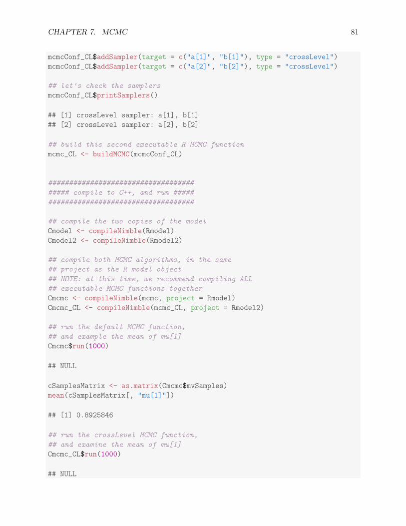
CHAPTER 7. MCMC 81
mcmcConf_CL$addSampler(target = c("a[1]", "b[1]"), type = "crossLevel")
mcmcConf_CL$addSampler(target = c("a[2]", "b[2]"), type = "crossLevel")
## let's check the samplers
mcmcConf_CL$printSamplers()
## [1] crossLevel sampler: a[1], b[1]
## [2] crossLevel sampler: a[2], b[2]
## build this second executable R MCMC function
mcmc_CL <- buildMCMC(mcmcConf_CL)
###################################
##### compile to C++, and run #####
###################################
## compile the two copies of the model
Cmodel <- compileNimble(Rmodel)
Cmodel2 <- compileNimble(Rmodel2)
## compile both MCMC algorithms, in the same
## project as the R model object
## NOTE: at this time, we recommend compiling ALL
## executable MCMC functions together
Cmcmc <- compileNimble(mcmc, project = Rmodel)
Cmcmc_CL <- compileNimble(mcmc_CL, project = Rmodel2)
## run the default MCMC function,
## and example the mean of mu[1]
Cmcmc$run(1000)
## NULL
cSamplesMatrix <- as.matrix(Cmcmc$mvSamples)
mean(cSamplesMatrix[, "mu[1]"])
## [1] 0.8925846
## run the crossLevel MCMC function,
## and examine the mean of mu[1]
Cmcmc_CL$run(1000)
## NULL

CHAPTER 7. MCMC 82
cSamplesMatrix_CL <- as.matrix(Cmcmc_CL$mvSamples)
mean(cSamplesMatrix_CL[, "mu[1]"])
## [1] 0.881214
###################################
#### run multiple MCMC chains #####
###################################
## run 3 chains of the crossLevel MCMC
samplesList <- runMCMC(Cmcmc_CL, niter=1000, nchains=3)
lapply(samplesList, dim)
## $chain1
## [1] 1000 2
##
## $chain2
## [1] 1000 2
##
## $chain3
## [1] 1000 2
7.11 Comparing different MCMCs with MCMCsuite and
compareMCMCs
NIMBLE’s MCMCsuite function automatically runs WinBUGS, OpenBUGS, JAGS, Stan,and/or multiple NIMBLE configurations on the same model. Note that the BUGS codemust be compatible with whichever BUGS packages are included, and separate Stan codemust be provided. NIMBLE’s compareMCMCs manages calls to MCMCsuite for multiple sets ofcomparisons and organizes the output(s) for generating html pages summarizing results. Italso allows multiple results to be combined and allows some different options for how resultsare processed, such as how effective sample size is estimated.
We first show how to use MCMCsuite for the same litters example used in Section 7.10.Subsequently, additional details of the MCMCsuite are given. Since use of compareMCMCs issimilar, we refer readers to help(compareMCMCs) and the functions listed under “See also”on that R help page.
7.11.1 MCMC Suite example: litters
The following code executes the following MCMC algorithms on the litters example:
1. WinBUGS

CHAPTER 7. MCMC 83
2. JAGS3. NIMBLE default configuration4. NIMBLE custom configuration using two crossLevel samplers
output <- MCMCsuite(
code = litters_code,
constants = constants,
data = data,
inits = inits,
monitors = 'mu',
MCMCs = c('winbugs', 'jags', 'nimble', 'nimble_CL'),
MCMCdefs = list(
nimble_CL = quote({mcmcConf <- configureMCMC(Rmodel, nodes = NULL)
mcmcConf$addSampler(target = c('a[1]', 'b[1]'),
type = 'crossLevel')
mcmcConf$addSampler(target = c('a[2]', 'b[2]'),
type = 'crossLevel')
mcmcConf
})),plotName = 'littersSuite'
)
7.11.2 MCMC Suite outputs
Executing the MCMC Suite returns a named list containing various outputs, as well asgenerates and saves traceplots and posterior density plots. The default elements of thisreturn list object are:
Samples
samples is a three-dimensional array, containing all MCMC samples from each algorithm.The first dimension of the samples array corresponds to each MCMC algorithm, and maybe indexed by the name of the algorithm. The second dimension of the samples arraycorresponds to each node which was monitored, and may be indexed by the node name.The third dimension of samples contains the MCMC samples, and has length niter/thin
- burnin.
Summary
The MCMC suite output contains a variety of pre-computed summary statistics, which arestored in the summary matrix. For each monitored node and each MCMC algorithm, thefollowing default summary statistics are calculated: mean, median, sd, the 2.5% quantile,and the 97.5% quantile. These summary statistics are easily viewable, as:
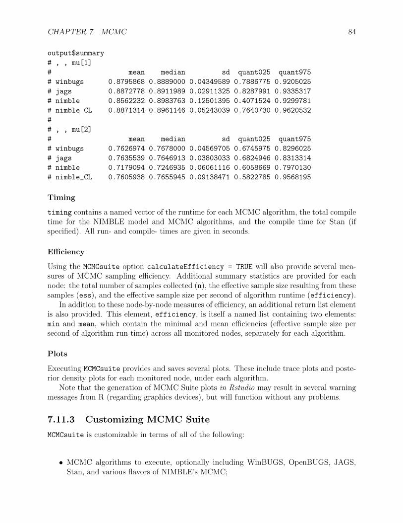
CHAPTER 7. MCMC 84
output$summary
# , , mu[1]
# mean median sd quant025 quant975
# winbugs 0.8795868 0.8889000 0.04349589 0.7886775 0.9205025
# jags 0.8872778 0.8911989 0.02911325 0.8287991 0.9335317
# nimble 0.8562232 0.8983763 0.12501395 0.4071524 0.9299781
# nimble_CL 0.8871314 0.8961146 0.05243039 0.7640730 0.9620532
#
# , , mu[2]
# mean median sd quant025 quant975
# winbugs 0.7626974 0.7678000 0.04569705 0.6745975 0.8296025
# jags 0.7635539 0.7646913 0.03803033 0.6824946 0.8313314
# nimble 0.7179094 0.7246935 0.06061116 0.6058669 0.7970130
# nimble_CL 0.7605938 0.7655945 0.09138471 0.5822785 0.9568195
Timing
timing contains a named vector of the runtime for each MCMC algorithm, the total compiletime for the NIMBLE model and MCMC algorithms, and the compile time for Stan (ifspecified). All run- and compile- times are given in seconds.
Efficiency
Using the MCMCsuite option calculateEfficiency = TRUE will also provide several mea-sures of MCMC sampling efficiency. Additional summary statistics are provided for eachnode: the total number of samples collected (n), the effective sample size resulting from thesesamples (ess), and the effective sample size per second of algorithm runtime (efficiency).
In addition to these node-by-node measures of efficiency, an additional return list elementis also provided. This element, efficiency, is itself a named list containing two elements:min and mean, which contain the minimal and mean efficiencies (effective sample size persecond of algorithm run-time) across all monitored nodes, separately for each algorithm.
Plots
Executing MCMCsuite provides and saves several plots. These include trace plots and poste-rior density plots for each monitored node, under each algorithm.
Note that the generation of MCMC Suite plots in Rstudio may result in several warningmessages from R (regarding graphics devices), but will function without any problems.
7.11.3 Customizing MCMC Suite
MCMCsuite is customizable in terms of all of the following:
• MCMC algorithms to execute, optionally including WinBUGS, OpenBUGS, JAGS,Stan, and various flavors of NIMBLE’s MCMC;

CHAPTER 7. MCMC 85
• custom-configured NIMBLE MCMC algorithms;• automated parameter blocking for efficient MCMC sampling;• nodes to monitor;• number of MCMC iterations;• thinning interval;• burn-in;• summary statistics to report;• calculating sampling efficiency (effective sample size per second of algorithm run-time);
and• generating and saving plots.
NIMBLE MCMC algorithms may be specified using the MCMCs argument to MCMCsuite,which is character vector defining the MCMC algorithms to run. The MCMCs argument mayinclude any of the following algorithms:
"winbugs" : WinBUGS MCMC algorithm"openbugs" : OpenBUGS MCMC algorithm"jags" : JAGS MCMC algorithm"Stan" : Stan default MCMC algorithm"nimble" : NIMBLE MCMC using the default configuration"nimble noConj" : NIMBLE MCMC using the default configuration with useConjugacy =
FALSE
"autoBlock" : NIMBLE MCMC algorithm with block sampling of dynamically determinedparameter groups attempting to maximize sampling efficiency
The default value for the MCMCs argument is "nimble", which specifies only the defaultNIMBLE MCMC algorithm.
The names of additional, custom, MCMC algorithms may also be provided in the MCMCs
argument, so long as these custom algorithms are defined in the MCMCdefs argument. Anexample of this usage is given with the crossLevel algorithm in the litters example in7.11.2.
The MCMCdefs argument should be a named list of definitions, for any custom MCMCalgorithms specified in the MCMCs argument. If MCMCs specified an algorithm called "myMCMC",then MCMCdefs must contain an element named "myMCMC". The contents of this element mustbe a block of code that, when executed, returns the desired MCMC configuration object.This block of code may assume the existence of the R model object, Rmodel. Further, thisblock of code need not worry about adding monitors to the MCMC configuration; it needonly specify the samplers.
As a final important point, execution of this block of code must return the MCMCconfiguration object. Therefore, elements supplied in the MCMCdefs argument should usuallytake the form:

CHAPTER 7. MCMC 86
MCMCdefs = list(
myMCMC = quote({mcmcConf <- configureMCMC(Rmodel, ....)
mcmcConf$addSampler(.....)
mcmcConf ## returns the MCMC configuration object
}))
Full details of the arguments and customization of the MCMC Suite is available viahelp(MCMCsuite).

Chapter 8
Sequential Monte Carlo and MCEM
The NIMBLE algorithm library is growing and as of version 0.6-7 includes a suite of Sequen-tial Monte Carlo algorithms as well as a more robust MCEM and k-fold cross-validation.
8.1 Particle Filters / Sequential Monte Carlo
8.1.1 Filtering Algorithms
NIMBLE includes algorithms for four different types of sequential Monte Carlo (also knownas particle filters), which can be used to sample from the latent states and approximate thelog likelihood of a state space model. The particle filters currently implemented in NIMBLEare the bootstrap filter, the auxiliary particle filter, the Liu-West filter, and the ensem-ble Kalman filter, which can be built, respectively, with calls to buildBootstrapFilter,buildAuxiliaryFilter, buildLiuWestFilter, and buildEnsembleKF. Each particle filterrequires setup arguments model and nodes; the latter should be a character vector specify-ing latent model nodes. In addition, each particle filter can be customized using a control
list argument. Details on the control options and specifics of the filtering algorithms can befound in the help pages for the functions.
Once built, each filter can be run by specifying the number of particles. Each filter hasa modelValues object named mvEWSamples that is populated with equally-weighted samplesfrom the posterior distribution of the latent states (and in the case of the Liu-West filter, theposterior distribution of the top level parameters as well) as the filter is run. The bootstrap,auxiliary, and Liu-West filters also have another modelValues object, mvWSamples, whichhas unequally-weighted samples from the posterior distribution of the latent states, alongwith weights for each particle. In addition, the bootstrap and auxiliary particle filters returnestimates of the log-likelihood of the given state space model.
We first create a linear state-space model to use as an example for our particle filteralgorithms.
## Building a simple linear state-space model.
## x is latent space, y is observed data
timeModelCode <- nimbleCode({
87
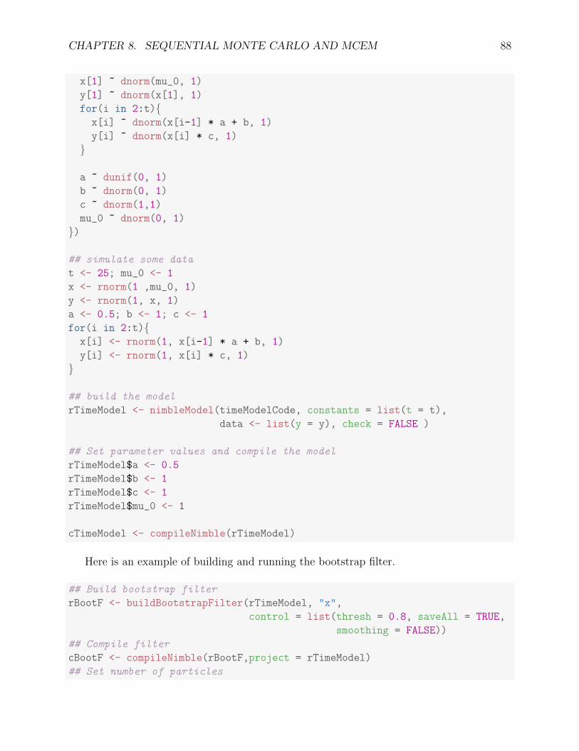
CHAPTER 8. SEQUENTIAL MONTE CARLO AND MCEM 88
x[1] ~ dnorm(mu_0, 1)
y[1] ~ dnorm(x[1], 1)
for(i in 2:t){x[i] ~ dnorm(x[i-1] * a + b, 1)
y[i] ~ dnorm(x[i] * c, 1)
}
a ~ dunif(0, 1)
b ~ dnorm(0, 1)
c ~ dnorm(1,1)
mu_0 ~ dnorm(0, 1)
})
## simulate some data
t <- 25; mu_0 <- 1
x <- rnorm(1 ,mu_0, 1)
y <- rnorm(1, x, 1)
a <- 0.5; b <- 1; c <- 1
for(i in 2:t){x[i] <- rnorm(1, x[i-1] * a + b, 1)
y[i] <- rnorm(1, x[i] * c, 1)
}
## build the model
rTimeModel <- nimbleModel(timeModelCode, constants = list(t = t),
data <- list(y = y), check = FALSE )
## Set parameter values and compile the model
rTimeModel$a <- 0.5
rTimeModel$b <- 1
rTimeModel$c <- 1
rTimeModel$mu_0 <- 1
cTimeModel <- compileNimble(rTimeModel)
Here is an example of building and running the bootstrap filter.
## Build bootstrap filter
rBootF <- buildBootstrapFilter(rTimeModel, "x",
control = list(thresh = 0.8, saveAll = TRUE,
smoothing = FALSE))
## Compile filter
cBootF <- compileNimble(rBootF,project = rTimeModel)
## Set number of particles

CHAPTER 8. SEQUENTIAL MONTE CARLO AND MCEM 89
parNum <- 5000
## Run bootstrap filter, which returns estimate of model log-likelihood
bootLLEst <- cBootF$run(parNum)
### The bootstrap filter can also return an estimate of the effective
### sample size (ESS) at each time point
bootESS <- cBootF$returnESS()
Next, we provide an example of building and running the auxiliary particle filter. Notethat a filter cannot be built on a model that already has a filter specialized to it, so we createa new copy of our state space model first.
## Copy our state-space model for use with the auxiliary filter
auxTimeModel <- rTimeModel$newModel(replicate = TRUE)
compileNimble(auxTimeModel)
## Build auxiliary filter
rAuxF <- buildAuxiliaryFilter(auxTimeModel, "x",
control = list(thresh = 0.5, saveAll = TRUE))
## Compile filter
cAuxF <- compileNimble(rAuxF,project = auxTimeModel)
## Run auxiliary filter, which returns estimate of model log-likelihood
auxLLEst <- cAuxF$run(parNum)
### The auxiliary filter can also return an estimate of the effective
### sample size (ESS) at each time point
auxESS <- cAuxF$returnESS()
Now we give an example of building and running the Liu and West filter, which can samplefrom the posterior distribution of top-level parameters as well as latent states. The Liu andWest filter accepts an additional params argument, specifying the top-level parameters tobe sampled.
## Copy model
LWTimeModel <- rTimeModel$newModel(replicate = TRUE)
compileNimble(LWTimeModel)
## Build Liu-West filter, also
## specifying which top level parameters to estimate
rLWF <- buildLiuWestFilter(LWTimeModel, "x", params = c("a", "b", "c"),
control = list(saveAll = FALSE))
## Compile filter
cLWF <- compileNimble(rLWF,project = LWTimeModel)
## Run Liu-West filter
cLWF$run(parNum)
Finally, we give an example of building and running the ensemble Kalman filter, whichcan sample from the posterior distribution of latent states.

CHAPTER 8. SEQUENTIAL MONTE CARLO AND MCEM 90
## Copy model
ENKFTimeModel <- rTimeModel$newModel(replicate = TRUE)
compileNimble(ENKFTimeModel)
## Build and compile ensemble Kalman filter
rENKF <- buildEnsembleKF(ENKFTimeModel, "x",
control = list(saveAll = FALSE))
cENKF <- compileNimble(rENKF,project = ENKFTimeModel)
## Run ensemble Kalman filter
cENKF$run(parNum)
Once each filter has been run, we can extract samples from the posterior distribution ofour latent states as follows:
## Equally-weighted samples (available from all filters)
bootEWSamp <- as.matrix(cBootF$mvEWSamples)
auxEWSamp <- as.matrix(cAuxF$mvEWSamples)
LWFEWSamp <- as.matrix(cLWF$mvEWSamples)
ENKFEWSamp <- as.matrix(cENKF$mvEWSamples)
## Unequally-weighted samples, along with weights (available
## from bootstrap, auxiliary, and Liu and West filters)
bootWSamp <- as.matrix(cBootF$mvWSamples, "x")
bootWts <- as.matrix(cBootF$mvWSamples, "wts")
auxWSamp <- as.matrix(xAuxF$mvWSamples, "x")
auxWts <- as.matrix(cAuxF$mvWSamples, "wts")
## Liu and West filter also returns samples
## from posterior distribution of top-level parameters:
aEWSamp <- as.matrix(cLWF$mvEWSamples, "a")
8.1.2 Particle MCMC (PMCMC)
Particle MCMC (PMCMC) is a method that uses MCMC for top-level model parametersand uses a particle filter to approximate the time-series likelihood for use in determiningMCMC acceptance probabilities [1]. NIMBLE implements PMCMC by providing random-walk Metropolis-Hastings samplers for model parameters that make use of particle filtersin this way. These samplers can use NIMBLE’s bootstrap filter or auxiliary particle filter,or they can use a user-defined filter. Whichever filter is specified will be used to obtainestimates of the likelihood of the state-space model (marginalizing over the latent states),which is used for calculation of the Metropolis-Hastings acceptance probability. The RW PF
sampler uses a univariate normal proposal distribution, and can be used to sample scalar top-level parameters. The RW PF block sampler uses a multivariate normal proposal distributionand can be used to jointly sample vectors of top-level parameters. The PMCMC samplers

CHAPTER 8. SEQUENTIAL MONTE CARLO AND MCEM 91
can be specified with a call to addSampler with type = "RW PF" or type = "RW PF block",a syntax similar to the other MCMC samplers listed in Section 7.9.
The RW PF sampler and RW PF block sampler can be customized using the control listargument to set the adaptive properties of the sampler and options for the particle filteralgorithm to be used. In addition, providing pfOptimizeNparticles=TRUE in the control
list will use an experimental algorithm to estimate the optimal number of particles to usein the particle filter. See help(samplers) for details. The MCMC configuration for thetimeModel in the previous section will serve as an example for the use of our PMCMCsampler. Here we use the identity matrix as our proposal covariance matrix.
timeConf <- configureMCMC(rTimeModel) # default MCMC configuration
## Add random walk PMCMC sampler with particle number optimization.
timeConf$addSampler(target = c("a", "b", "c", "mu_0"), type = "RW_PF_block",
control <- list(propCov= diag(4), adaptScaleOnly = FALSE,
latents = "x", pfOptimizeNparticles = TRUE))
The type = "RW PF" and type = "RW PF block" samplers default to using a bootstrapfilter. However, more efficient results can often be obtained by using a custom filteringalgorithm. Choice of filtering algorithm can be controlled by the pfType control list entry.The pfType entry can be set either to ’bootstrap’ (the default), ’auxiliary’, or the nameof a user-defined nimbleFunction that returns a likelihood approximation.
Any user-defined filtering nimbleFunction named in the pfType control list entry mustsatsify the following:
1. The nimbleFunction must be the result of a call to nimbleFunction().2. The nimbleFunction must have setup code that accepts the following (and only the
following) arguments:
• model, the nimble model object that the MCMC algorithm is defined on.• latents, a character vector specifying the latent model nodes over which the par-
ticle filter will stochastically integrate over to estimate the log-likelihood function.• control, an R list object. Note that the control list can be used to pass in any
additional information or arguments that the custom filter may require.
3. The nimbleFunction must have a run function that accepts a single integer arug-ment (the number of particles to use), and returns a scalar double (the log-likelihoodestimate).
4. The nimbleFunction must define, in setup code, a modelValues object named mvEWSamples
that is used to contain equally weighted samples of the latent states (that is, thelatents argument to the setup function). Each time the run() method of the nimbleFunctionis called with number of particles m, the mvEWSamples modelValues object should beresized to be of size m via a call to resize(mvEWSamples, m).

CHAPTER 8. SEQUENTIAL MONTE CARLO AND MCEM 92
8.2 Monte Carlo Expectation Maximization (MCEM)
Suppose we have a model with missing data (or a layer of latent variables that can be treatedas missing data), and we would like to maximize the marginal likelihood of the model,integrating over the missing data. A brute-force method for doing this is MCEM. This is anEM algorithm in which the missing data are simulated via Monte Carlo (often MCMC, whenthe full conditional distributions cannot be directly sampled from) at each iteration. MCEMcan be slow, and there are other methods for maximizing marginal likelihoods that can beimplemented in NIMBLE. The reason we started with MCEM is to explore the flexibility ofNIMBLE and illustrate the ability to combine R and NIMBLE to run an algorithm, withR managing the highest-level processing of the algorithm and calling nimbleFunctions forcomputations.
NIMBLE provides an ascent-based MCEM algorithm, created using buildMCEM, thatautomatically determines when the algorithm has converged by examining the size of thechanges in the likelihood between each iteration. Additionally, the MCEM algorithm canprovide an estimate of the asymptotic covariance matrix of the parameters. An example ofcalculating the asymptotic covariance can be found in Section 8.2.1.
We will revisit the pump example to illustrate the use of NIMBLE’s MCEM algorithm.
pump <- nimbleModel(code = pumpCode, name = "pump", constants = pumpConsts,
data = pumpData, inits = pumpInits, check = FALSE)
compileNimble(pump)
## build an MCEM algorithm with ascent-based convergence criterion
pumpMCEM <- buildMCEM(model = pump,
latentNodes = "theta", burnIn = 300,
mcmcControl = list(adaptInterval = 100),
boxConstraints = list( list( c("alpha", "beta"),
limits = c(0, Inf) ) ),
buffer = 1e-6)
The first argument buildMCEM, model, is a NIMBLE model, which can be either theuncompiled or compiled version. At the moment, the model provided cannot be part ofanother MCMC sampler. The ascent-based MCEM algorithm has a number of controloptions:
The latentNodes argument should indicate the nodes that will be integrated over (sam-pled via MCMC), rather than maximized. These nodes must be stochastic, not deterministic!latentNodes will be expanded as described in Section 13.3.1. I.e., either latentNodes =
"x" or latentNodes = c("x[1]", "x[2]") will treat x[1] and x[2] as latent nodes if x
is a vector of two values. All other non-data nodes will be maximized over. Note thatlatentNodes can include discrete nodes, but the nodes to be maximized cannot.
The burnIn argument indicates the number of samples from the MCMC for the E-stepthat should be discarded when computing the expected likelihood in the M-step. Note that

CHAPTER 8. SEQUENTIAL MONTE CARLO AND MCEM 93
burnIn can be set to values lower than in standard MCMC computations, as each iterationwill start where the last left off.
The mcmcControl argument will be passed to configureMCMC to define the MCMC tobe used.
The MCEM algorithm automatically detects box constraints for the nodes that will beoptimized, using NIMBLE’s getBounds function. It is also possible for a user to manuallyspecify constraints via the boxConstraints argument. Each constraint given should be alist in which the first element is the names of the nodes or variables that the constraint willbe applied to and the second element is a vector of length two, in which the first value isthe lower limit and the second is the upper limit. Values of Inf and -Inf are allowed. Ifa node is not listed, its constraints will be automatically determined by NIMBLE. Theseconstraint arguments are passed as the lower and upper arguments to R’s optim function,using method = "L-BFGS-B". Note that NIMBLE will give a warning if a user-providedconstraint is more extreme than the constraint determined by NIMBLE.
The value of the buffer argument shrinks the boxConstraints by this amount. Thiscan help protect against non-finite values occurring when a parameter is on the boundary.
In addition, the MCEM has some extra control options that can be used to further tunethe convergence criterion. See help(buildMCEM) for more information.
The buildMCEM function returns a list with two elements. The first element is a functioncalled run, which will use the MCEM algorithm to estimate the MLEs. The second functionis called estimateCov, and is described in Section 8.2.1. The run function can be runas follows. There is only one run-time argument, initM, which is the number of MCMCiterations to use when the algorithm is initialized.
pumpMLE <- pumpMCEM$run(initM = 1000)
## Iteration Number: 1.
## Current number of MCMC iterations: 1000.
## Parameter Estimates:
## alpha beta
## 0.8209063 1.1454658
## Convergence Criterion: 1.001.
## Iteration Number: 2.
## Current number of MCMC iterations: 1000.
## Parameter Estimates:
## alpha beta
## 0.8139532 1.2087601
## Convergence Criterion: 0.01644723.
## Monte Carlo error too big: increasing MCMC sample size.
## Iteration Number: 3.
## Current number of MCMC iterations: 1350.
## Parameter Estimates:
## alpha beta
## 0.8128915 1.2250123
## Convergence Criterion: 0.001898588.

CHAPTER 8. SEQUENTIAL MONTE CARLO AND MCEM 94
## Iteration Number: 4.
## Current number of MCMC iterations: 1350.
## Parameter Estimates:
## alpha beta
## 0.8214914 1.2520907
## Convergence Criterion: 0.00160825.
## Monte Carlo error too big: increasing MCMC sample size.
## Iteration Number: 5.
## Current number of MCMC iterations: 1875.
## Parameter Estimates:
## alpha beta
## 0.8222741 1.2612285
## Convergence Criterion: 0.0004661995.
pumpMLE
## alpha beta
## 0.8222741 1.2612285
Direct maximization after analytically integrating over the latent nodes (possible for thismodel but often not feasible) gives estimates of α = 0.823 and β = 1.261, so the MCEMseems to do pretty well, though tightening the convergence criteria may be warranted inactual usage.
8.2.1 Estimating the Asymptotic Covariance From MCEM
The second element of the list returned by a call to buildMCEM is a function called estimateCov,which estimates the asymptotic covariance of the parameters at their MLE values. If therun function has been called previously, the estimateCov function will automatically usethe MLE values produced by the run function to estimate the covariance. Alternatively,a user can supply their own MLE values using the MLEs argument, which allows the co-variance to be estimated without having called the run function. More details about theestimateCov function can be found by calling help(buildMCEM). Below is an example ofusing the estimateCov function.
pumpCov <- pumpMCEM$estimateCov()
pumpCov
## alpha beta
## alpha 0.1255779 0.2111345
## beta 0.2111345 0.6164128
##alternatively, you can manually specify the MLE values as a named vector.
pumpCov <- pumpMCEM$estimateCov(MLEs = c(alpha = 0.823, beta = 1.261))
Chapter 9
Spatial models
NIMBLE supports two variations of conditional autoregressive (CAR) model structures: theimproper intrinsic Gaussian CAR (ICAR) model, and a proper Gaussian CAR model. Thisincludes distributions to represent these spatially-dependent model structures in a BUGSmodel, as well as specialized MCMC samplers for these distributions.
9.1 Intrinsic Gaussian CAR model: dcar normal
The intrinsic Gaussian conditional autoregressive (ICAR) model used to model dependenceof block-level values (e.g., spatial areas or temporal blocks) is implemented in NIMBLE asthe dcar normal distribution. Additional details for using this distribution are availableusing help(’CAR-Normal’).
ICAR models are improper priors for random fields (e.g., temporal or spatial processes).The prior is a joint prior across a collection of latent process values. For more technicaldetails on CAR models, including higher-order CAR models, please see [17], [2], and [15].Since the distribution is improper it should not be used as the distribution for data values,but rather to specify a prior for an unknown process. As discussed in the references above,the distribution can be seen to be a proper density in a reduced dimension subspace; thusthe impropriety only holds on one or more linear combinations of the latent process values.
In addition to our focus here on CAR modeling for spatial data, the ICAR model canalso be used in other contexts, such as for temporal data in a discrete time context.
9.1.1 Specification and density
NIMBLE uses the same parameterization as WinBUGS / GeoBUGS for the dcar normal
distribution, providing compatibility with existing WinBUGS code. NIMBLE also providesthe WinBUGS name car.normal as an alias.
Specification
The dcar normal distribution is specified for a set of N spatially dependent regions as:
x[1:N] ∼ dcar normal(adj, weights, num, tau, c, zero mean)
95

CHAPTER 9. SPATIAL MODELS 96
The adj, weights and num parameters define the adjacency structure and associatedweights of the spatially-dependent field. See help(CAR-Normal) for details of these param-eters. When specifying a CAR distribution, these parameters must have constant values.They do not necessarily have to be specified as constants when creating a model objectusing nimbleModel, but they should be defined in a static way: as right-hand-side onlyvariables with initial values provided as constants, data or inits, or using fixed numericaldeterministic declarations. Each of these two approaches for specifying values are shown inthe example.
The adjacency structure defined by adj and the associated weights must be symmetric.That is, if region i is neighbor of region j, then region j must also be a neighbor of regioni. Further, the weights associated with these reciprocating relationships must be equal.NIMBLE performs a check of these symmetries and will issue an error message if asymmetryis detected.
The scalar precision tau may be treated as an unknown model parameter and itselfassigned a prior distribution. Care should be taken in selecting a prior distribution for tau,and WinBUGS suggests that users be prepared to carry out a sensitivity analysis for thischoice.
When specifying a higher-order CAR process, the number of constraints c can be explic-itly provided in the model specification. This would be the case, for example, when specifyinga thin-plate spline (second-order) CAR model, for which c should be 2 for a one-dimensionalprocess and 3 for a two-dimensional (e.g., spatial) process, as discussed in [17] and [15]. Ifc is omitted, NIMBLE will calculate c as the number of disjoint groups of regions in theadjacency structure, which implicitly assumes a first-order CAR process for each group.
By default there is no zero-mean constraint imposed on the CAR process, and thus themean is implicit within the CAR process values, with an implicit improper flat prior onthe mean. To avoid non-identifiability, one should not include an additional parameter forthe mean (e.g., do not include an intercept term in a simple CAR model with first-orderneighborhood structure). When there are disjoint groups of regions and the constraint isnot imposed, there is an implicit distinct improper flat prior on the mean for each group,and it would not make sense to impose the constraint since the constraint holds across allregions. Similarly, if one sets up a neighborhood structure for higher-order CAR models, itwould not make sense to impose the zero-mean constraint as that would account for onlyone of the eigenvalues that are zero. Imposing this constraint (by specifying the parameterzero mean = 1) allows users to model the process mean separately, and hence a separateintercept term should be included in the model.
NIMBLE provides a convenience function as.carAdjacency for converting other repre-sentations of the adjacency information into the required adj, weights, num format. Thisfunction can convert:
• A symmetric adjacency matrix of weights (with diagonal elements equal to zero), usingas.carAdjacency(weightMatrix)
• Two length-N lists with numeric vector elements giving the neighboring indices and as-sociated weights for each region, using as.carAdjacency(neighborList, weightList)
These conversions should be done in R, and the resulting adj, weights, num vectors canbe passed as constants into nimbleModel.

CHAPTER 9. SPATIAL MODELS 97
Density
For process values x = (x1, . . . , xN) and precision τ , the improper CAR density is given as:
p(x|τ) ∝ τ (N−c)/2 e−τ2
∑i 6=j wij (xi−xj)2
where the summation over all (i, j) pairs, with the weight between regions i and j given bywij, is equivalent to summing over all pairs for which region i is a neighbor of region j. Notethat the value of c modifies the power to which the precision is raised, accounting for theimpropriety of the density based on the number of zero eigenvalues in the implicit precisionmatrix for x.
For the purposes of MCMC sampling the individual CAR process values, the resultingconditional prior of region i is:
p(xi|x−i, τ) ∼ N(
1wi+
∑j∈Ni wij xj, wi+τ
)where x−i represents all elements of x except xi, the neighborhood Ni of region i is theset of all j for which region j is a neighbor of region i, wi+ =
∑j∈Ni wij, and the Normal
distribution is parameterized in terms of precision.
9.1.2 Example
Here we provide an example model using the intrinsic Gaussian dcar normal distribution.The CAR process values are used in a spatially-dependent Poisson regression.
To mimic the behavior of WinBUGS, we specify zero mean = 1 to enforce a zero-meanconstraint on the CAR process, and therefore include a separate intercept term alpha inthe model. Note that we do not necessarily recommend imposing this constraint, per thediscussion earlier in this chapter.
code <- nimbleCode({alpha ~ dflat()
beta ~ dnorm(0, 0.0001)
tau ~ dgamma(0.001, 0.001)
for(k in 1:L)
weights[k] <- 1
s[1:N] ~ dcar_normal(adj[1:L], weights[1:L], num[1:N], tau, zero_mean = 1)
for(i in 1:N) {log(lambda[i]) <- alpha + beta*x[i] + s[i]
y[i] ~ dpois(lambda[i])
}})
constants <- list(N = 4, L = 8, num = c(3, 2, 2, 1),
adj = c(2,3,4,1,3,1,2,1), x = c(0, 2, 2, 8))
data <- list(y = c(6, 9, 7, 12))
inits <- list(alpha = 0, beta = 0, tau = 1, s = c(0, 0, 0, 0))

CHAPTER 9. SPATIAL MODELS 98
Rmodel <- nimbleModel(code, constants, data, inits)
The resulting model may be carried through to MCMC sampling. NIMBLE will assigna specialized sampler to the update the elements of the CAR process. See chapter 7 forinformation about NIMBLE’s MCMC engine, and section 9.3 for details MCMC samplingof the CAR processes.
9.2 Proper Gaussian CAR model: dcar proper
The proper Gaussian conditional autoregressive model used to model dependence of block-level values (e.g., spatial areas or temporal blocks) is implemented in NIMBLE as thedcar proper distribution. Addition details of using this distribution are available usinghelp(’CAR-Proper’).
Proper CAR models are proper priors for random fields (e.g., temporal or spatial pro-cesses). The prior is a joint prior across a collection of latent process values. For moretechnical details on proper CAR models please see [2], including considerations of why theimproper CAR model may be preferred.
In addition to our focus here on CAR modeling for spatial data, the proper CAR modelcan also be used in other contexts, such as for temporal data in a discrete time context.
9.2.1 Specification and density
NIMBLE uses the same parameterization as WinBUGS / GeoBUGS for the dcar proper
distribution, providing compatibility with existing WinBUGS code. NIMBLE also providesthe WinBUGS name car.proper as an alias.
Specification
The dcar proper distribution is specified for a set of N spatially dependent regions as:
x[1:N] ∼ dcar proper(mu, C, adj, num, M, tau, gamma)
There is no option of a zero-mean constraint for proper CAR process, and instead themean for each region is specified by the mu parameter. The elements of mu can be assignedfixed values or may be specified using one common, or multiple, prior distributions.
The C, adj, num and M parameters define the adjacency structure, normalized weights, andconditional variances of the spatially-dependent field. See help(CAR-Proper) for details ofthese parameters. When specifying a CAR distribution, these parameters must have constantvalues. They do not necessarily have to be specified as constants when creating a modelobject using nimbleModel, but they should be defined in a static way: as right-hand-side onlyvariables with initial values provided as constants, data or inits, or using fixed numericaldeterministic declarations.
The adjacency structure defined by adj must be symmetric. That is, if region i is neigh-bor of region j, then region j must also be a neighbor of region i. In addition, the normalized

CHAPTER 9. SPATIAL MODELS 99
weights specified in C must satisfy a symmetry constraint jointly with the conditional vari-ances given in M. This constraint requires that M−1C is symmetric, where M is a diagonalmatrix of conditional variances and C is the normalized (each row sums to one) weight ma-trix. Equivalently, this implies that CijMjj = CjiMii for all pairs of neighboring regions iand j. NIMBLE performs a check of these symmetries and will issue an error message ifasymmetry is detected.
Two options are available to simplify the process of constructing the C and M arguments;both options are demonstrated in the example. First, these arguments may be omittedfrom the dcar proper specification. In this case, values of C and M will be generated thatcorrespond to all weights being equal to one, or equivalently, a symmetric weight matrixcontaining only zeros and ones. Note that C and M should either both be provided, or bothbe omitted from the specification.
Second, a convenience function as.carCM is provided to generate the C and M argumentscorresponding to a specified set of symmetric unnormalized weights. If weights containsthe non-zero weights corresponding to an unnormalized weight matrix (weights is preciselythe argument that can be used in the dcar normal specification), then a list containing C
and M can be generated using as.carCM(adj, weights, num). In this case, the resulting C
contains the row-normalized weights, and the resulting M is a vector of the inverse row-sumsof the unnormalized weight matrix.
The scalar precision tau may be treated as an unknown model parameter and itselfassigned a prior distribution. Care should be taken in selecting a prior distribution for tau,and WinBUGS suggests that users be prepared to carry out a sensitivity analysis for thischoice.
An appropriate value of the gamma parameter ensures the propriety of the dcar proper
distribution. The value of gamma must lie between fixed bounds, which are given by thereciprocals of the largest and smallest eigenvalues of M−1/2CM1/2. These bounds can becalculated using the function carBounds or separately using the functions carMinBound
and carMaxBound. For compatibility with WinBUGS, NIMBLE provides min.bound andmax.bound as aliases for carMinBound and carMaxBound. Rather than selecting a fixedvalue of gamma within these bounds, it is recommended that gamma be assigned a uniformprior distribution over the region of permissible values.
Note that when C and M are omitted from the dcar proper specification (and hence allweights are taken as one), or C and M are calculated from a symmetric weight matrix usingthe utility function as.carCM, then the bounds on gamma are necessarily (−1, 1). In thiscase, gamma can simply be assigned a prior over that region. This approach is shown in bothexamples.
Density
The proper CAR density is given as:
p(x|µ,C,M, τ, γ) ∼ MVN(µ, 1
τ(I − γC)−1M
)where the multivariate normal distribution is parameterized in terms of covariance.
For the purposes of MCMC sampling the individual CAR process values, the resultingconditional prior of region i is:

CHAPTER 9. SPATIAL MODELS 100
p(xi|x−i, µ, C,M, τ, γ) ∼ N(µi +
∑j∈Ni γ Cij (xj − µi), Mii
τ
)where x−i represents all elements of x except xi, the neighborhood Ni of region i is the set ofall j for which region j is a neighbor of region i, and the Normal distribution is parameterizedin terms of variance.
9.2.2 Example
We provide two example models using the proper Gaussian dcar proper distribution. Inboth, the CAR process values are used in a spatially-dependent logistic regression to modelbinary presence/absence data. In the first example, the C and M parameters are omitted,which uses weights equal to one for all neighbor relationships. In the second example,symmetric unnormalized weights are specified, and as.carCM is used to construct the C andM parameters to the dcar proper distribution.
## omitting C and M sets all non-zero weights to one
code <- nimbleCode({mu0 ~ dnorm(0, 0.0001)
tau ~ dgamma(0.001, 0.001)
gamma ~ dunif(-1, 1)
s[1:N] ~ dcar_proper(mu[1:N], adj=adj[1:L], num=num[1:N], tau=tau,
gamma=gamma)
for(i in 1:N) {mu[i] <- mu0
logit(p[i]) <- s[i]
y[i] ~ dbern(p[i])
}})
adj <- c(2, 1, 3, 2, 4, 3)
num <- c(1, 2, 2, 1)
constants <- list(adj = adj, num = num, N = 4, L = 6)
data <- list(y = c(1, 0, 1, 1))
inits <- list(mu0 = 0, tau = 1, gamma = 0, s = rep(0, 4))
Rmodel <- nimbleModel(code, constants, data, inits)
## specify symmetric unnormalized weights, use as.carCM to generate C and M
code <- nimbleCode({mu0 ~ dnorm(0, 0.0001)
tau ~ dgamma(0.001, 0.001)
gamma ~ dunif(-1, 1)
s[1:N] ~ dcar_proper(mu[1:N], C[1:L], adj[1:L], num[1:N], M[1:N], tau,
gamma)
for(i in 1:N) {

CHAPTER 9. SPATIAL MODELS 101
mu[i] <- mu0
logit(p[i]) <- s[i]
y[i] ~ dbern(p[i])
}})
weights <- c(2, 2, 3, 3, 4, 4)
CM <- as.carCM(adj, weights, num)
constants <- list(C = CM$C, adj = adj, num = num, M = CM$M, N = 4, L = 6)
Rmodel <- nimbleModel(code, constants, data, inits)
Each of the resulting models may be carried through to MCMC sampling. NIMBLEwill assign a specialized sampler to update the elements of the CAR process. See Chapter7 for information about NIMBLE’s MCMC engine, and Section 9.3 for details on MCMCsampling of the CAR processes.
9.3 MCMC Sampling of CAR models
NIMBLE’s MCMC engine provides specialized samplers for the dcar normal and dcar proper
distributions. These samplers perform sequential univariate updates on the components ofthe CAR process. Internally, each sampler assigns one of three specialized univariate sam-plers to each component, based on inspection of the model structure:
1. A conjugate sampler in the case of conjugate Normal dependencies.2. A random walk Metropolis-Hastings sampler in the case of non-conjugate dependencies.3. A posterior predictive sampler in the case of no dependencies.
Note that these univariate CAR samplers are not the same as NIMBLE’s standardconjugate, RW, and posterior predictive samplers, but rather specialized versions foroperating on a CAR distribution. Details of these assignments are strictly internal to theCAR samplers.
In future versions of NIMBLE we expect to provide block samplers that update theentire CAR process as a single sample. This may provide improved MCMC performance byaccounting for dependence between elements, particularly when conjugacy is available.
9.3.1 Initial values
Valid initial values should be provided for all elements of the process specified by a CARstructure before running an MCMC. This ensures that the conditional prior distribution iswell-defined for each region. A simple and safe choice of initial values is setting all compo-nents of the process equal to zero, as is done in the preceding CAR examples.
For compatibility with WinBUGS, NIMBLE also allows an initial value of NA to be pro-vided for regions with zero neighbors. This particular initialization is required in WinBUGS,so this allows users to make use of existing WinBUGS code.

CHAPTER 9. SPATIAL MODELS 102
9.3.2 Zero-neighbor regions
Regions with zero neighbors (defined by a 0 appearing in the num parameter) are a special casefor both the dcar normal and dcar proper distribution. The corresponding neighborhoodN of such a region contains no elements, and hence the conditional prior is improper anduninformative, tantamount to a dflat prior distribution. Thus, the conditional posteriordistribution of those regions is entirely determined by the dependent nodes, if any. Samplingof these zero-neighbor regions proceeds as:
• In the conjugate case, sampling proceeds according to the conjugate posterior.• In the non-conjugate case, sampling proceeds using random walk Metropolis-Hastings,
where the posterior is determined entirely by the dependencies.• In the case of no dependents, the posterior is entirely undefined. Here, no changes will
be made to the process value, and it will remain equal to its initial value throughout. Byvirtue of having no neighbors, this region does not contribute to the density evaluationof the subsuming dcar normal node nor to the conditional prior of any other regions,hence its value (even NA) is of no consequence.
This behavior is different from that of WinBUGS, where the value of zero-neighbor regionsof car.normal nodes is set to and fixed at zero.
9.3.3 Zero-mean constraint
A zero-mean constraint is available for the intrinsic Gaussian dcar normal distribution. Thisconstraint on the ICAR process values is imposed during MCMC sampling, if the argumentzero mean = 1, mimicking the behavior of WinBUGS. Following the univariate updates oneach component, the mean is subtracted away from all process values, resulting in a zero-mean process.
Note that this is not equivalent to sampling under the constraint that the mean is zero(see p. 36 of [17]) so should be treated as an ad hoc approach and employed with caution.

Chapter 10
Bayesian nonparametric models
As of version 0.6-11, NIMBLE provides initial support for Bayesian nonparametric (BNP)mixture modeling. These features are currently considered EXPERIMENTAL – please letus know (via the NIMBLE user mailing list or by emailing us) if you have any problems orhave suggestions about functionality you would like NIMBLE to support or the NIMBLEinterface for using BNP.
10.1 Bayesian nonparametric mixture models
NIMBLE provides support for Bayesian nonparametric (BNP) mixture modeling. The cur-rent implementation provides support for hierarchical specifications involving Dirichlet pro-cess (DP) mixtures [6, 7, 11, 4, 5]. More specifically, a DP mixture model takes the form
yi | Giid∼∫h(yi | θ)G(dθ),
G | α,G0 ∼ DP (α,G0),
where h(· | θ) is a suitable kernel with parameter θ, and α and G0 are the concentration andbaseline distribution parameters of the DP, respectively. DP mixture models can be writtenwith different levels of hierarchy, all being equivalent to the model above.
When the random measure G is integrated out from the model, the DP mixture modelcan be written using latent or membership variables, zi, following a Chinese RestaurantProcess (CRP) distribution [3], discussed in Section 10.2. The model takes the form
yi | θ, ziind∼ h(· | θzi),
z | α ∼ CRP(α), θjiid∼ G0,
where CRP(α) denotes the CRP distribution with concentration parameter α.If a stick-breaking representation [18], discussed in section 10.3, is assumed for the random
measure G, then the model takes the form
yi | θ?,vind∼
∞∑l=1
{vl∏m<l
(1− vm)
}h(· | θ?l ),
103

CHAPTER 10. BAYESIAN NONPARAMETRIC MODELS 104
vl | αiid∼ Beta(1, α), θ?l
iid∼ G0.
More general representations of the random measure can be specify by considering vl |νl, αl
ind∼ Beta(νl, αl). Finite dimensional approximations can be obtained by truncating theinfinite sum to have L components.
Different representations of DP mixtures lead to different computational algorithms.NIMBLE supports sampling algorithms based on the CRP representation, as well as onthe stick-breaking representation. NIMBLE includes definitions of structures required toimplement the CRP and stick-breaking distributions, and the associated MCMC algorithms.
10.2 Chinese Restaurant Process model
The CRP is a distribution over the space of partitions of positive integers and is implementedin NIMBLE as the dCRP distribution. More details for using this distribution are availableusing help(CRP).
The CRP can be described as a stochastic process in which customers arrive at a restau-rant, potentially with an infinite number of tables. Each customer sits at an empty oroccupied table according to probabilities that depend on the number of customers in theoccupied tables. Thus, the CRP partitions the set of customers, through their assignmentto tables in the restaurant.
10.2.1 Specification and density
NIMBLE parametrizes the dCRP distribution by a concentration parameter and a size pa-rameter.
Specification
The dCRP distribution is specified in NIMBLE for a membership vector z as
z[1:N] ∼ dCRP(conc, size)
The conc parameter is the concentration parameter of the CRP, controlling the proba-bility of a customer sitting on a new table, i.e., creating a new cluster. The size parameterdefines the size of the set of integers to be partitioned.
The conc parameter is a positive real value that can be treated as known or unknown.When a gamma prior is assumed for the conc parameter, a specialized sampler is assigned.See more on this in section 10.4.1.
The size parameter is a positive integer that has to be fixed and equal to the lengthof vector z. It defines the set of consecutive integers from 1 to N to be partitioned. Eachelement in z can be an integer from 1 to N, and repetitions are allowed.

CHAPTER 10. BAYESIAN NONPARAMETRIC MODELS 105
Density
The CRP distribution partitions the set of positive integers {1, . . . , N}, into N? ≤ N disjointsubsets, indicating to which subset each element belongs. For instance, if N = 6, theset {1, 2, 3, 4, 5, 6} can be partitioned into the subsets S1 = {1, 2, 6}, S2 = {4, 5}, andS3 = {3}. Note that N? = 3, and this is one partition from out of 203 possibilities. The CRP-distributed vector z encodes this partition and its observed values would be (1, 1, 3, 2, 2, 1),for this example. In mixture modeling, this indicates that observations 1, 2, and 6 belongto cluster 1, observations 4 and 5 to cluster 2, and observation 3 to cluster 3. Note that thisrepresentation is not unique, vector (2, 2, 1, 3, 3, 2) encodes the same partition.
The joint probability function of z = (z1, . . . , zN), with concentration parameter α, isgiven by
p(z | α) ∝ Γ(α)
Γ(α + n)αN
?(z)
N?(z)∏k=1
Γ(mk(z)),
where mk(z) denotes the number of elements in z that are equal to k. The full conditionaldistribution for zi given z−i is
p(zi = m | z−i, α) =1
n− 1 + α
∑j 6=i
1{zj}(m) +α
n− 1 + α1{znew}(m),
where z−i denotes vector z after removing its i−th component, znew is a value not in z−i,and 1A denotes the indicator function at set A.
Note that the probability of creating a new cluster is proportional to α: the larger theconcentration parameter, the more clusters are created.
10.2.2 Example
The following example illustrates how to use NIMBLE to perform single density estimationfor real-valued data, under a BNP approach, using the dCRP distribution. (Note that theBNP approach is also often used to perform density estimation on random effects.) Themodel is given by
yi | θ, σ2, ziind∼ N(θzi , σ
2zi, ) i = 1, . . . , N,
z ∼ CRP(α), α ∼ Gamma(1, 1),
θjiid∼ N(0, 100), σ2
jiid∼ InvGamma(1, 1), j = 1, . . . ,M.
code <- nimbleCode({z[1:N] ~ dCRP(alpha, size = N)
alpha ~ dgamma(1, 1)
for(i in 1:M) {thetatilde[i] ~ dnorm(0, 100)
s2tilde[i] ~ dinvgamma(1, 1)

CHAPTER 10. BAYESIAN NONPARAMETRIC MODELS 106
}for(i in 1:N)
y[i] ~ dnorm(thetatilde[z[i]], var = s2tilde[z[i]])
})
set.seed(1)
constants <- list(N = 100, M = 50)
data <- list(y = c(rnorm(50, -5, sqrt(3)), rnorm(50, 5, sqrt(4))))
inits <- list(thetatilde = rnorm(constants$N, 0, 10),
s2tilde = rinvgamma(constants$N, 1, 1),
z = sample(1:10, size = constants$N, replace = TRUE),
alpha = 1)
Rmodel <- nimbleModel(code, constants, data, inits)
The resulting model may be fitted through MCMC sampling. NIMBLE will assign aspecialized sampler to update z and alpha. See chapter 7 for information about NIMBLE’sMCMC engine, and section 10.4.1 for details on MCMC sampling of the CRP.
One of the advantages of BNP mixture models is that the number of clusters is treated asrandom. Therefore, in MCMC sampling, the number of cluster parameters varies with theiteration. Since NIMBLE does not currently allow dynamic length allocation, the numberof unique cluster parameters, N?, has to be fixed. One safe option is to set this number toN , but this is inefficient, both in terms of computation and in terms of storage, because inpractice it is often that N? < N . In addition, configuring and building the MCMC can beslow (and use a lot of memory) for large M . In an effort to mitigate these inefficiencies, weallow the user to set N? = M , with M < N , as seen in the example above. However, if thisnumber is too small and is exceeded in any iteration a warning is issued.
10.3 Stick-breaking model
In NIMBLE, weights defined by sequentially breaking a stick, as in the stick-breaking process,are implemented as the stick breaking link function. More details for using this functionare available using help(stick breaking).
10.3.1 Specification and function
NIMBLE parametrizes the stick breaking function by vector of values in (0, 1).
Function
The weights (w1, . . . , wL) follow a finite stick-breaking construction if
w1 = v1,
wl = vl∏m<l
(1− vm), l = 2, . . . , L− 1

CHAPTER 10. BAYESIAN NONPARAMETRIC MODELS 107
wL =∏m<L
(1− vm).
for vl ∈ [0, 1], l = 1, . . . , L− 1.
Specification
The stick breaking function is specified in NIMBLE for a vector w of probabilities as
w[1:L] <- stick breaking(v[1:(L-1)])
The argument v is a vector of values between 0 and 1 defining the sequential breakingpoints of the stick after removing the previous portions already broken off. It is of lengthL− 1, implicitly assuming that its last component is equal to 1.
In order to complete the definition of the weights in the stick-breaking representation ofG, a prior distribution on (0, 1) should to be assumed for vl, l = 1, . . . , L− 1, for instance abeta prior.
10.3.2 Example
Here we illustrate how to use NIMBLE for the example described in section 10.2.2, butconsidering a stick-breaking representation for G. The model is given by
yi | θ?,σ?2, ziind∼ N(θ?zi , σ
2?zi
), i = 1, . . . , N,
z ∼ Discrete(w), vliid∼ Beta(1, α), l = 1, . . . , L− 1,
α ∼ Gamma(1, 1),
θ?liid∼ N(0, 100), σ2?
liid∼ InvGamma(1, 1), l = 1, . . . , L.
where w1 = v1, wl = vl∏
m<l(1− vm), for l = 1, . . . , L− 1, and wL =∏
m<L(1− vm).
code <- nimbleCode({for(i in 1:(L-1)){
v[i] ~ dbeta(1, alpha)
}alpha ~ dgamma(1, 1)
w[1:L] <- stick_breaking(v[1:(L-1)])
for(i in 1:L) {thetastar[i] ~ dnorm(0, 100)
s2star[i] ~ dinvgamma(1, 1)
}for(i in 1:N) {
z[i] ~ dcat(w[1:L])
y[i] ~ dnorm(thetastar[z[i]], var = s2star[z[i]])
}

CHAPTER 10. BAYESIAN NONPARAMETRIC MODELS 108
})
set.seed(1)
constants <- list(N = 100, L=50)
data <- list(y = c(rnorm(50, -5, sqrt(3)), rnorm(50, 5, sqrt(4))))
inits <- list(thetastar = rnorm(constants$L, 0, 100),
s2star = rinvgamma(constants$L, 1, 1),
z = sample(1:10, size = constants$N, replace = TRUE),
v = rbeta(constants$L, 1, 1),
alpha = 1)
RmodelSB <- nimbleModel(code, constants, data, inits)
The resulting model may be carried through to MCMC sampling. NIMBLE will assigna specialized sampler to update v. See chapter 7 for information about NIMBLE’s MCMCengine, and section 10.4.2 for details on MCMC sampling of the stick-breaking weights.
10.4 MCMC sampling of BNP models
BNP models can be specified in different, yet equivalent, manners. Examples 10.2.2 and10.3.2 are examples of density estimation for real-valued data, and are specified through theCRP and the stick-breaking process, respectively. Different specifications lead NIMBLE toassign different sampling algorithms for the model. When the model is specified through aCRP, a collapsed sampler [13] is assigned. Under this specification, the random measure Gis integrated out from the model. When a stick-breaking representation is used, a blockedGibbs sampler is assigned, see [9] and [10].
10.4.1 Sampling CRP models
NIMBLE’s MCMC engine provides specialized samplers for the dCRP distribution, updatingeach component of the membership vector sequentially. Internally, the sampler is assignedbased on inspection of the model structure, evaluating conjugacy between the mixture kerneland the baseline distribution, as follows:
1. A conjugate sampler in the case of the baseline distribution being conjugate for themixture kernel.
2. A non-conjugate sampler in the case of the baseline distribution not being conjugatefor the mixture kernel.
Note that both samplers are specialized versions that operate on a vector having a CRPdistribution. Details of these assignments are strictly internal to the CRP samplers. Ad-ditionally, a specialized sampler is assigned to the conc hyper parameter when a gammahyper prior is assigned, see section 6 in [5] for more details. Otherwise, a random walkMetropolis-Hastings sampler is assigned.
CHAPTER 10. BAYESIAN NONPARAMETRIC MODELS 109
Initial values
Valid initial values should be provided for all elements of the process specified by a CRPstructure before running the MCMC. A simple and safe choice for z is to provide a sampleof size N, the same as its length, of values between 1 and some reasonable number of clusters(less than or equal to the length of z), with replacement, as done in the preceding CRPexample. For the concentration parameter, a safe initial value is 1.
Sampling the random measure
In BNP models, it is oftenly of interest to make inference about the unknown measure G.NIMBLE provides a sampler, getSamplesDPmeasure, for this random measure when a CRPstructure is involved in the model.
The argument of the getsamplesDPmeasure function is a compiled or uncompiled MCMCobject. The MCMC object should monitor the membership (clustering) variable, the clusterparameters, all stochastic nodes of the cluster parameters, and the concentration parameter,if it is random. Use the monitors argument when configuring the MCMC to ensure thesevariables are monitored in the MCMC.
The sampler is used only after the MCMC for the model has been run; more details areavailable from help(getsamplesDPmeasure).
The following code exemplifies how to generate samples from G after defining the modelas in section 10.2.2.
cRmodel <- compileNimble(Rmodel)
monitors <- c('z', 'thetatilde', 's2tilde' , 'alpha')
RmodelConf <- configureMCMC(Rmodel, monitors = monitors)
RmodelMCMC <- buildMCMC(RmodelConf)
CmodelMCMC <- compileNimble(RmodelMCMC, project = Rmodel)
CmodelMCMC$run(1000)
samplesG <- getSamplesDPmeasure(CmodelMCMC)
10.4.2 Sampling stick-breaking models
NIMBLE’s MCMC engine provides specialized samplers for the beta-distributed randomvariables that are the arguments to the stick-breaking function, updating each componentof the weight vector sequentially. The sampler is assigned based on inspection of the modelstructure. Specifically, the specialized sampler is assigned when the membership vector hasa categorical distribution, its weights are defined by a stick-breaking function, and the vectordefining the weights follows a beta distribution.

CHAPTER 10. BAYESIAN NONPARAMETRIC MODELS 110
Initial values
Valid initial values should be provided for all elements of the stick-breaking function andmembership variable before running the MCMC. A simple and safe choice for z is to providea sample of size N, of values between 1 and some value less than L, with replacement, asdone in the preceding stick-breaking example. For the stick variables, safe initial values canbe simulated from a beta distribution.

Part IV
Programming with NIMBLE
111

112
Part IV is the programmer’s guide to NIMBLE. At the heart of programming in NIMBLEare nimbleFunctions. These support two principal features: (1) a setup function that is runonce for each model, nodes, or other setup arguments, and (2) run functions that will becompiled to C++ and are written in a subset of R enhanced with features to operate models.Formally, what can be compiled comprises the NIMBLE language, which is designed to beR-like.
This part of the manual is organized as follows:
• Chapter 11 describes how to write simple nimbleFunctions, which have no setup codeand hence don’t interact with models, to compile parts of R for fast calculations. Thiscovers the subset of R that is compilable, how to declare argument types and returntypes, and other information.• Chapter 12 explains how to write nimbleFunctions that can be included in BUGS code
as user-defined distributions or user-defined functions.• Chapter 13 introduces more features of NIMBLE models that are useful for writing
nimbleFunctions to use models, focusing on how to query model structure and carryout model calculations.• Chapter 14 introduces two kinds of data structures: modelValues are used for holding
multiple sets of values of model variables; nimbleList data structures are similar toR lists but require fixed element names and types, allowing the NIMBLE compiler touse them.• Chapter 15 draws on the previous chapters to show how to write nimbleFunctions
that work with models, or more generally that have a setup function for any purpose.Typically a setup function queries model structure (Chapter 13) and may establishsome modelValues or nimbleList data structures or configurations (Chapter 14).Then run functions written in the same way as simple nimbleFunctions (Chapter 11)along with model operations (Chapter 13) define algorithm computations that can becompiled via C++.

Chapter 11
Writing simple nimbleFunctions
11.1 Introduction to simple nimbleFunctions
nimbleFunctions are the heart of programming in NIMBLE. In this chapter, we introducesimple nimbleFunctions that contain only one function to be executed, in either compiled oruncompiled form, but no setup function or additional methods.
Defining a simple nimbleFunction is like defining an R function: nimbleFunction returnsa function that can be executed, and it can also be compiled. Simple nimbleFunctions areuseful for doing math or the other kinds of processing available in NIMBLE when no modelor modelValues is needed. These can be used for any purpose in R programming. They canalso be used as new functions and distributions in NIMBLE’s extension of BUGS (Chapter12).
Here’s a basic example implementing the textbook calculation of least squares estimationof linear regression parameters1:
solveLeastSquares <- nimbleFunction(
run = function(X = double(2), y = double(1)) { ## type declarations
ans <- inverse(t(X) %*% X) %*% (t(X) %*% y)
return(ans)
returnType(double(2)) ## return type declaration
} )
X <- matrix(rnorm(400), nrow = 100)
y <- rnorm(100)
solveLeastSquares(X, y)
## [,1]
## [1,] 0.15448951
## [2,] 0.02707736
## [3,] -0.05432358
## [4,] -0.05100693
1Of course, in general, explicitly calculating the inverse is not the recommended numerical recipe for leastsquares.
113
CHAPTER 11. WRITING SIMPLE NIMBLEFUNCTIONS 114
CsolveLeastSquares <- compileNimble(solveLeastSquares)
CsolveLeastSquares(X, y)
## [,1]
## [1,] 0.15448951
## [2,] 0.02707736
## [3,] -0.05432358
## [4,] -0.05100693
In this example, we fit a linear model for 100 random response values (y) to four columnsof randomly generated explanatory variables (X). We ran the nimbleFunction solveLeastSquares
uncompiled, natively in R, allowing testing and debugging (Section 15.7). Then we com-piled it and showed that the compiled version does the same thing, but faster2. NIMBLE’scompiler creates C++ that uses the Eigen (http://eigen.tuxfamily.org) library for linearalgebra.
Notice that the actual NIMBLE code is written as an R function definition that is passedto nimbleFunction as the run argument. Hence we call it the run code. run code is writtenin the NIMBLE language. This is similar to a narrow subset of R with some additionalfeatures. Formally, we view it as a distinct language that encompasses what can be compiledfrom a nimbleFunction.
To write nimbleFunctions, you will need to learn:
• what R functions are supported for NIMBLE compilation and any ways they differfrom their regular R counterparts;• how NIMBLE handles types of variables;• how to declare types of nimbleFunction arguments and return values;• that compiled nimbleFunctions always pass arguments to each other by reference.
The next sections cover each of these topics in turn.
11.2 R functions (or variants) implemented in NIM-
BLE
11.2.1 Finding help for NIMBLE’s versions of R functions
Often, R help pages are available for NIMBLE’s versions of R functions using the prefix“nim” and capitalizing the next letter. For example, help on NIMBLE’s version of numericcan be found by help(nimNumeric). In some cases help is found directly using the name ofthe function as it appears in R.
2On the machine this is being written on, the compiled version runs a few times faster than the uncompiledversion. However we refrain from formal speed tests.

CHAPTER 11. WRITING SIMPLE NIMBLEFUNCTIONS 115
11.2.2 Basic operations
Basic R operations supported for NIMBLE compilation are listed in Table 11.1.
CHAPTER 11. WRITING SIMPLE NIMBLEFUNCTIONS 116
Table 11.1: Basic R manipulation functions in NIMBLE. To find help in R for NIMBLE’s version of afunction, use the “nim” prefix and capitalize the next letter. E.g. help(nimC) for help with c().
Function Comments (differences from R)
c() No recursive argument.rep() No rep.int or rep len arguments.seq() and ‘:’ Negative integer sequences from ‘:’, e.g. 2:1, do not work.seq along()
which() No arr.ind or useNames arguments.diag() Works like R in three ways: diag(vector) returns a matrix with vector
on the diagonal; diag(matrix) returns the diagonal vector of matrix; diag(n) returns ann× n identity matrix. No nrow or ncol arguments.
diag()<- Works for assigning the diagonal vector of a matrix.dim() Works on a vector as well as higher-dimensional arguments.length()
is.na() Does not correctly handle NAs from R that are type ’logical’, so convert these using as.numeric()
before passing from R to NIMBLE.is.nan()
numeric() Allows additional arguments to control initialization.logical() Allows additional arguments to control initialization.integer() Allows additional arguments to control initialization.matrix() Allows additional arguments to control initialization.array() Allows additional arguments to control initialization.indexing Arbitrary integer and logical indexing is supported for objects of one or two dimensions.
For higher-dimensional objects, only ‘:‘ indexing works and then only to create an objectof at most two dimensions.
Other R functions with numeric arguments and return value can be called during compiledexecution by wrapping them as a nimbleRcall (see Section 11.7).
Next we cover some of these functions in more detail.
numeric, integer, logical, matrix and array
numeric, integer, or logical will create a 1-dimensional vector of floating-point (or “dou-ble” [precision]), integer, or logical values, respectively. The length argument specifies thevector length (default 0), and the value argument specifies the initial value either as a scalar(used for all vector elements, with default 0) or a vector. If a vector and its length is not equalto length, the remaining values will be zero, but we plan to implement R-style recycling inthe next version of NIMBLE. The init argument specifies whether or not to initialize theelements in compiled code (default TRUE). If first use of the variable does not rely on initialvalues, using init = FALSE will yield slightly more efficient performance.
matrix creates a 2-dimensional matrix object of either floating-point (if type = "double",the default), integer (if type = "integer"), or logical (if type = "logical") values. Asin R, nrow and ncol arguments specify the number of rows and columns, respectively. Thevalue and init arguments are used in the same way as for numeric, integer, and logical.
array creates a vector or higher-dimensional object, depending on the dim argument,which takes a vector of sizes for each dimension. The type, value and init argumentbehave the same as for matrix.

CHAPTER 11. WRITING SIMPLE NIMBLEFUNCTIONS 117
The best way to create an identity matrix is with diag(n), which returns an n × nidentity matrix. NIMBLE also provides a deprecated nimbleFunction identityMatrix thatdoes the same thing.
Examples of these functions, and the related function setSize for changing the size of anumeric object, are given in Section 11.3.2.
length and dim
length behaves like R’s length function. It returns the entire length of X. That means ifX is multivariate, length(X) returns the product of the sizes of the dimensions. NIMBLE’sversion of dim, which has synonym nimDim, behaves like R’s dim function for matrices orarrays and like R’s length function for vectors. In other words, regardless of whether thenumber of dimensions is 1 or more, it returns a vector of the sizes.
Deprecated creation of non-scalar objects using declare
Previous versions of NIMBLE provided a function declare for declaring variables. The moreR-like functions numeric, integer, logical, matrix and array are intended to replacedeclare, but declare is still supported for backward compatibility. In a future version ofNIMBLE, declare may be removed.
11.2.3 Math and linear algebra
Numeric scalar and matrix mathematical operations are listed in Tables 11.2 and 11.3.As in R, many scalar operations in NIMBLE will work component-wise on vectors or
higher dimensional objects. For example if B and C are vectors, A = B + C will add themand create vector C by component-wise addition of B and C. In the current version ofNIMBLE, component-wise operations generally only work for vectors and matrices, notarrays with more than two dimensions. The only exception is assignment: A = B will workup to NIMBLE’s current limit of four dimensions.
Table 11.2: Functions operating on scalars, many of which can operate on each element (component-wise)of vectors and matrices. Status column indicates if the function is currently provided in NIMBLE.
Usage Description Comments Status Acceptsvector input
x | y, x & y logical OR (|) and AND(&) ! !
!x logical not ! !
x > y, x >= y greater than (and or equal to) ! !
x < y, x <= y less than (and or equal to) ! !
x != y, x == y (not) equals ! !
x + y, x - y, x * y component-wise operators mix of scalar and vector ok ! !
x / y, component-wise division vector x and scalar y ok ! !
x^y, pow(x, y) power xy; vector x and scalar y ok ! !
x %% y modulo (remainder) !
min(x1, x2), min. (max.) of two scalars ! See pmin, pmax

CHAPTER 11. WRITING SIMPLE NIMBLEFUNCTIONS 118
Table 11.2: Functions operating on scalars, many of which can operate on each element (component-wise)of vectors and matrices. Status column indicates if the function is currently provided in NIMBLE.
Usage Description Comments Status Acceptsvector input
max(x1, x2)
exp(x) exponential ! !
log(x) natural logarithm ! !
sqrt(x) square root ! !
abs(x) absolute value ! !
step(x) step function at 0 0 if x < 0, 1 if x >= 0 ! !
equals(x, y) equality of two scalars 1 if x == y, 0 if x! = y !
cube(x) third power x3 ! !
sin(x), cos(x), tan(x) trigonometric functions ! !
asin(x), acos(x), inverse trigonometric functions ! !atan(x)
asinh(x), acosh(x), inv. hyperbolic trig. functions ! !atanh(x)
logit(x) logit log(x/(1− x)) ! !
ilogit(x), expit(x) inverse logit exp(x)/(1 + exp(x)) ! !
probit(x) probit (Gaussian quantile) Φ−1(x) ! !
iprobit(x), phi(x) inverse probit (Gaussian CDF) Φ(x) ! !
cloglog(x) complementary log log log(− log(1− x)) ! !
icloglog(x) inverse complementary log log 1− exp(− exp(x)) ! !
ceiling(x) ceiling function d(x)e ! !
floor(x) floor function b(x)c ! !
round(x) round to integer ! !
trunc(x) truncation to integer ! !
lgamma(x), loggam(x) log gamma function log Γ(x) ! !
besselK(x, nu, modified bessel function ! !expon.scaled) of the second kind
log1p(x) log of 1 + x log(1 + x) ! !
lfactorial(x), log factorial log x! ! !logfact(x)
log1p(x) log one-plus log(x+ 1) ! !
qDIST(x, PARAMS) “q” distribution functions canonical parameterization ! !
pDIST(x, PARAMS) “p” distribution functions canonical parameterization ! !
rDIST(1, PARAMS) “r” distribution functions canonical parameterization ! !
dDIST(x, PARAMS) “d” distribution functions canonical parameterization ! !sort(x)
rank(x, s)
ranked(x, s)
order(x)

CHAPTER 11. WRITING SIMPLE NIMBLEFUNCTIONS 119
Table 11.3: Functions operating on vectors and matrices. Status column indicates if the function is currentlyprovided in NIMBLE.
Usage Description Comments Status
inverse(x) matrix inverse x symmetric, positive definite !
chol(x) matrix Cholesky factorization x symmetric, positive definite !
t(x) matrix transpose x> !
x%*%y matrix multiply xy; x, y conformant !
inprod(x, y) dot product x>y; x and y vectors !
solve(x, y) solve system of equations x−1y; y matrix or vector !
forwardsolve(x, y) solve lower-triangular system of equations x−1y; x lower-triangular !
backsolve(x, y) solve upper-triangular system of equations x−1y; x upper-triangular !
logdet(x) log matrix determinant log |x| !
asRow(x) convert vector x to 1-row matrix sometimes automatic !
asCol(x) convert vector x to 1-column matrix sometimes automatic !
sum(x) sum of elements of x !
mean(x) mean of elements of x !
sd(x) standard deviation of elements of x !
prod(x) product of elements of x !
min(x), max(x) min. (max.) of elements of x !
pmin(x, y), pmax(x, y) vector of mins (maxs) of elements of x and y !interp.lin(x, v1, v2) linear interpolation
eigen(x) matrix eigendecomposition x symmetric, returns a nimbleList !of type eigenNimbleList
svd(x) matrix singular value decomposition returns a nimbleList of type !svdNimbleList
More information on the nimbleLists returned by the eigen and svd functions in NIM-BLE can be found in Section 14.2.1.
11.2.4 Distribution functions
Distribution “d”, “r”, “p”, and “q” functions can all be used from nimbleFunctions (and inBUGS model code), but care is needed in the syntax, as follows.
• Names of the distributions generally (but not always) match those of R, which some-times differ from BUGS. See the list below.• Supported parameterizations are also indicated in the list below.• For multivariate distributions (multivariate normal, Dirichlet, and Wishart), “r” func-
tions only return one random draw at a time, and the first argument must always be1.• R’s recycling rule (re-use of an argument as needed to accommodate longer values of
other arguments) is generally followed, but the returned object is always a scalar or avector, not a matrix or array.
As in R (and nimbleFunctions), arguments are matched by order or by name (if given).Standard arguments to distribution functions in R (log, log.p, lower.tail) can be used

CHAPTER 11. WRITING SIMPLE NIMBLEFUNCTIONS 120
and have the same defaults. User-defined distributions for BUGS (Chapter 12) can also beused from nimbleFunctions.
For standard distributions, we rely on R’s regular help pages (e.g., help(dgamma). Fordistributions unique to NIMBLE (e.g., dexp nimble, ddirch), we provide help pages.
Supported distributions, listed by their “d” function, include:
• dbinom(x, size, prob, log)
• dcat(x, prob, log)
• dmulti(x, size, prob, log)
• dnbinom(x, size, prob, log)
• dpois(x, lambda, log)
• dbeta(x, shape1, shape2, log)
• dchisq(x, df, log)
• dexp(x, rate, log)
• dexp nimble(x, rate, log)
• dexp nimble(x, scale, log)
• dgamma(x, shape, rate, log)
• dgamma(x, shape, scale, log)
• dinvgamma(x, shape, rate, log)
• dinvgamma(x, shape, scale, log)
• dlnorm(x, meanlog, sdlog, log)
• dlogis(x, location, scale, log)
• dnorm(x, mean, sd, log)
• dt nonstandard(x, df, mu, sigma,
log)
• dt(x, df, log)
• dunif(x, min, max, log)
• dweibull(x, shape, scale, log)
• ddirch(x, alpha, log)
• dmnorm chol(x, mean, cholesky,
prec param, log)
• dmvt chol(x, mu, cholesky, df,
prec param, log)
• dwish chol(x, cholesky, df,
scale param, log)
In the last three, cholesky stands for Cholesky decomposition of the relevant matrix;prec param is a logical indicating whether the Cholesky is of a precision matrix (TRUE) orcovariance matrix (FALSE)3; and scale param is a logical indicating whether the Choleskyis of a scale matrix (TRUE) or an inverse scale matrix (FALSE).
11.2.5 Flow control: if-then-else, for, while, and stop
These basic flow-control structures use the same syntax as in R. However, for-loops arelimited to sequential integer indexing. For example, for(i in 2:5) {...} works as itdoes in R. Decreasing index sequences are not allowed. Unlike in R, if is not itself afunction that returns a value.
We plan to include more flexible for-loops in the future, but for now we’ve included justone additional useful feature: for(i in seq along(NFL)) will work as in R, where NFL isa nimbleFunctionList. This is described in Section 15.4.8.
stop, or equivalently nimStop, throws control to R’s error-handling system and can takea character argument that will be displayed in an error message.
11.2.6 print and cat
print, or equivalently nimPrint, prints an arbitrary set of outputs in order and adds anewline character at the end. cat or nimCat is identical, except without a newline at theend.
3For the multivariate t, these are more properly termed the ‘inverse scale’ and ‘scale’ matrices.
CHAPTER 11. WRITING SIMPLE NIMBLEFUNCTIONS 121
11.2.7 Checking for user interrupts: checkInterrupt
When you write algorithms that will run for a long time in C++, you may want to explicitlycheck whether a user has tried to interrupt the execution (i.e., by pressing Control-C). Simplyinclude checkInterrupt in run code at places where a check should be done. If there hasbeen an interrupt waiting to be handled, the process will stop and return control to R.
11.2.8 Optimization: optim and nimOptim
NIMBLE provides a nimOptim function that partially implement’s R’s optim function withsome minor differences. nimOptim supports optimization methods “Nelder-Mead”, “BFGS”,“CG”, “L-BFGS-B”, but does not support methods “SANN” and “Brent”. NIMBLE’snimOptim supports gradients using user-provided functions if available or finite differencesotherwise, but it does not currently support Hessian computations. Currently nimOptim
does not support extra parameters to the function being optimized (via ...), but a work-around is to create a new nimbleFunction that binds those fixed parameters. Finally,nimOptim requires a nimbleList datatype for the control parameter, whereas R’s optim
uses a simple R list. To define the control parameter, create a default value with thenimOptimDefaultControl function, and set any desired fields. For example usage, see theunit tests in tests/test-optim.R.
11.2.9 “nim” synonyms for some functions
NIMBLE uses some keywords, such as dim and print, in ways similar but not identical to R.In addition, there are some keywords in NIMBLE that have the same names as R functionswith quite different functionality. For example, step is part of the BUGS language, but it isalso an R function for stepwise model selection. And equals is part of the BUGS languagebut is also used in the testthat package, which we use in testing NIMBLE.
NIMBLE tries to avoid conflicts by replacing some keywords immediately upon creatinga nimbleFunction. These replacements include
• c → nimC
• copy → nimCopy
• dim → nimDim
• print → nimPrint
• cat → nimCat
• step → nimStep
• equals → nimEquals
• rep → nimRep
• round → nimRound
• seq → nimSeq
• stop → nimStop
• switch → nimSwitch
• numeric, integer, logical →nimNumeric, nimInteger, nimLogical
• matrix, array → nimMatrix,
nimArray
This system gives programmers the choice between using the keywords like nimPrint
directly, to avoid confusion in their own code about which “print” is being used, or to usethe more intuitive keywords like print but remember that they are not the same as R’sfunctions.

CHAPTER 11. WRITING SIMPLE NIMBLEFUNCTIONS 122
11.3 How NIMBLE handles types of variables
Variables in the NIMBLE language are statically typed. Once a variable is used for one type,it can’t subsequently be used for a different type. This rule facilitates NIMBLE’s compilationto C++. The NIMBLE compiler often determines types automatically, but sometimes theprogrammer needs to explicitly provide them.
The elemental types supported by NIMBLE include double (floating-point), integer, logi-cal, and character. The type of a numeric or logical object refers to the number of dimensionsand the elemental type of the elements. Hence if x is created as a double matrix, it can onlybe used subsequently for a double matrix. The size of each dimension is not part of itstype and thus can be changed. Up to four dimensions are supported for double, integer,and logical. Only vectors (one dimension) are supported for character. Unlike R, NIMBLEsupports true scalars, which have 0 dimensions.
11.3.1 nimbleList data structures
A nimbleList is a data structure that can contain arbitrary other NIMBLE objects, includ-ing other nimbleLists. Like other NIMBLE types, nimbleLists are strongly typed: eachnimbleList is created from a configuration that declares what types of objects it will hold.nimbleLists are covered in Chapter 14.2.
11.3.2 How numeric types work
R’s dynamic types support easy programming because one type can sometimes be trans-formed to another type automatically when an expression is evaluated. NIMBLE’s statictypes makes it stricter than R.
When NIMBLE can automatically set a numeric type
When a variable is first created by assignment, its type is determined automatically by thatassignment. For example, if x has not appeared before, then
x <- A %*% B ## assume A and B are double matrices or vectors
will create x to be a double matrix of the correct size (determined during execution). Ifx is used subsequently, it can only be used as a double matrix. This is true even if it isassigned a new value, which will again set its size automatically but cannot change its type.
When a numeric object needs to be created before being used
If the contents of a variable are to be populated by assignment into some indices in steps,the variable must be created first. Further, it must be large enough for its eventual contents;it will not be automatically resized if assignments are made beyond its current size. Forexample, in the following code, x must be created before being filled with contents forspecific indices.

CHAPTER 11. WRITING SIMPLE NIMBLEFUNCTIONS 123
x <- numeric(10)
for(i in 1:10)
x[i] <- foo(y[i])
Changing the sizes of existing objects: setSize
setSize changes the size of an object, preserving its contents in column-major order.
## Example of creating and resizing a floating-point vector
## myNumericVector will be of length 10, with all elements initialized to 2
myNumericVector <- numeric(10, value = 2)
## resize this numeric vector to be length 20; last 10 elements will be 0
setSize(myNumericVector, 20)
## Example of creating a 1-by-10 matrix with values 1:10 and resizing it
myMatrix <- matrix(1:10, nrow = 1, ncol = 10)
## resize this matrix to be a 10-by-10 matrix
setSize(myMatrix, c(10, 10))
## The first column will have the 1:10
Confusions between scalars and length-one vectors
In R, there is no such thing is a true scalar; scalars can always be treated as vectors of lengthone. NIMBLE allows true scalars, which can create confusions. For example, consider thefollowing code:
myfun <- nimbleFunction(
run = function(i = integer()) { ## i is an integer scalar
randomValues <- rnorm(10) ## double vector
a <- randomValues[i] ## double scalar
b <- randomValues[i:i] ## double vector
d <- a + b ## double vector
f <- c(i) ## integer vector
})
In the line that creates b, the index range i:i is not evaluated until run time. Eventhough i:i will always evaluate to simpy i, the compiler does not determine that. Sincethere is a vector index range provided, the result of randomValues[i:i] is determined tobe a vector. The following line then creates d as a vector, because a vector plus a scalarreturns a vector. Another way to create a vector from a scalar is to use c, as illustrated inthe last line.

CHAPTER 11. WRITING SIMPLE NIMBLEFUNCTIONS 124
Confusions between vectors and one-column or one-row matrices
Consider the following code:
myfun <- nimbleFunction(
run = function() {A <- matrix(value = rnorm(9), nrow = 3)
B <- rnorm(3)
Cmatrix <- A %*% B ## double matrix, one column
Cvector <- (A %*% B)[,1] ## double vector
Cmatrix <- (A %*% B)[,1] ## error, vector assigned to matrix
Cmatrix[,1] <- (A %*% B)[,1] ## ok, if Cmatrix is large enough
})
This creates a matrix A, a vector B, and matrix-multiplies them. The vector B is au-tomatically treated as a one-column matrix in matrix algebra computations. The result ofmatrix multiplication is always a matrix, but a programmer may expect a vector, since theyknow the result will have one column. To make it a vector, simply extract the first column.More information about such handling is provided in the next section.
Understanding dimensions and sizes from linear algebra
As much as possible, NIMBLE behaves like R when determining types and sizes returnedfrom linear algebra expressions, but in some cases this is not possible because R uses run-timeinformation while NIMBLE must determine dimensions at compile time. For example, whenmatrix multiplying a matrix by a vector, R treats the vector as a one-column matrix unlesstreating it as a one-row matrix is the only way to make the expression valid, as determined atrun time. NIMBLE usually must assume during compilation that it should be a one-columnmatrix, unless it can determine not just the number of dimensions but the actual sizes duringcompilation. When needed asRow and asCol can control how a vector will be treated as amatrix.
Here is a guide to such issues. Suppose v1 and v2 are vectors, and M1 is a matrix. Then
• v1 + M1 generates a compilation error unless one dimension of M1 is known at compile-time to be 1. If so, then v1 is promoted to a 1-row or 1-column matrix to conformwith M1, and the result is a matrix of the same sizes. This behavior occurs for allcomponent-wise binary functions.• v1 %*% M1 defaults to promoting v1 to a 1-row matrix, unless it is known at compile-
time that M1 has 1 row, in which case v1 is promoted to a 1-column matrix.• M1 %*% v1 defaults to promoting v1 to a 1-column matrix, unless it is known at compile
time that M1 has 1 column, in which case v1 is promoted to a 1-row matrix.• v1 %*% v2 promotes v1 to a 1-row matrix and v2 to a 1-column matrix, so the returned
values is a 1x1 matrix with the inner product of v1 and v2. If you want the innerproduct as a scalar, use inprod(v1, v2).• asRow(v1) explicitly promotes v1 to a 1-row matrix. Therefore v1 %*% asRow(v2)
gives the outer product of v1 and v2.

CHAPTER 11. WRITING SIMPLE NIMBLEFUNCTIONS 125
• asCol(v1) explicitly promotes v1 to a 1-column matrix.• The default promotion for a vector is to a 1-column matrix. Therefore, v1 %*% t(v2)
is equivalent to v1 %*% asRow(v2) .• When indexing, dimensions with scalar indices will be dropped. For example, M1[1,]
and M1[,1] are both vectors. If you do not want this behavior, use drop=FALSE justas in R. For example, M1[1,,drop=FALSE] is a matrix.• The left-hand side of an assignment can use indexing, but if so it must already be
correctly sized for the result. For example, Y[5:10, 20:30] <- x will not work – andcould crash your R session with a segmentation fault – if Y is not already at least 10x30in size. This can be done by setSize(Y, c(10, 30)). See Section 11.3.2 for moredetails. Note that non-indexed assignment to Y, such as Y <- x, will automatically setY to the necessary size.
Here are some examples to illustrate the above points, assuming M2 is a square matrix.
• Y <- v1 + M2 %*% v2 will return a 1-column matrix. If Y is created by this statement,it will be a 2-dimensional variable. If Y already exists, it must already be 2-dimesional,and it will be automatically re-sized for the result.• Y <- v1 + (M2 %*% v2)[,1] will return a vector. Y will either be created as a vector
or must already exist as a vector and will be re-sized for the result.
Size warnings and the potential for crashes
For matrix algebra, NIMBLE cannot ensure perfect behavior because sizes are not knownuntil run time. Therefore, it is possible for you to write code that will crash your R session.In Version 0.6-11, NIMBLE attempts to issue a warning if sizes are not compatible, but itdoes not halt execution. Therefore, if you execute A <- M1 % * % M2, and M1 and M2 arenot compatible for matrix multiplication, NIMBLE will output a warning that the numberof rows of M1 does not match the number of columns of M2. After that warning the statementwill be executed and may result in a crash. Another easy way to write code that will crash isto do things like Y[5:10, 20:30] <- x without ensuring Y is at least 10x30. In the futurewe hope to prevent crashes, but in Version 0.6-11 we limit ourselves to trying to provideuseful information.
11.4 Declaring argument and return types
NIMBLE requires that types of arguments and the type of the return value be explicitlydeclared.
As illustrated in the example in Section 11.1, the syntax for a type declaration is:type(nDim, sizes)
where type is double, integer, logical or character. (In more general nimbleFunctionprogramming, a type can also be a nimbleList type, discussed in Section 14.2.)
For example run = function(x = double(1)) ... sets the single argument of therun function to be a vector of numeric values of unknown size.

CHAPTER 11. WRITING SIMPLE NIMBLEFUNCTIONS 126
For type(nDim, sizes), nDim is the number of dimensions, with 0 indicating scalar andomission of nDim defaulting to a scalar. sizes is an optional vector of fixed, known sizes.For example, double(2, c(4, 5)) declares a 4-×-5 matrix. If sizes are omitted, they willbe set either by assignment or by setSize.
In the case of scalar arguments only, a default value can be provided. For example, toprovide 1.2 as a default:
myfun <- nimbleFunction(
run = function(x = double(0, default = 1.2)) {})
Functions with return values must have their return type explicitly declared using returnType,which can occur anywhere in the run code. For example returnType(integer(2)) declaresthe return type to be a matrix of integers. A return type of void() means there is no returnvalue, which is the default if no returnType statement is included.
11.5 Compiled nimbleFunctions pass arguments by ref-
erence
Uncompiled nimbleFunctions pass arguments like R does, by copy. If x is passed as anargument to function foo, and foo modifies x internally, it is modifying its copy of x, notthe original x that was passed to it.
Compiled nimbleFunctions pass arguments to other compiled nimbleFunctions by refer-ence (or pointer). This is very different. Now if foo modifies x internally, it is modifyingthe same x that was passed to it. This allows much faster execution but is obviously afundamentally different behavior.
Uncompiled execution of nimbleFunctions is primarily intended for debugging. However,debugging of how nimbleFunctions interact via arguments requires testing the compiledversions.
11.6 Calling external compiled code
If you have a function in your own compiled C or C++ code and an appropriate header file,you can generate a nimbleFunction that wraps access to that function, which can then beused in other nimbleFunctions. See help(nimbleExternalCall) for an example. This alsocontains an example of using an externally compiled function in the BUGS code of a model.
11.7 Calling uncompiled R functions from compiled
nimbleFunctions
Sometimes one may want to combine R functions with compiled nimbleFunctions. Obviouslya compiled nimbleFunction can be called from R. An R function with numeric inputs and

CHAPTER 11. WRITING SIMPLE NIMBLEFUNCTIONS 127
output can be called from compiled nimbleFunctions. The call to the R function is wrappedin a nimbleFunction returned by nimbleRcall. See help(nimbleRcall) for an example,including an example of using the resulting function in the BUGS code of a model.

Chapter 12
Creating user-defined BUGSdistributions and functions
NIMBLE allows you to define your own functions and distributions as nimbleFunctions foruse in BUGS code. As a result, NIMBLE frees you from being constrained to the functionsand distributions discussed in Chapter 5. For example, instead of setting up a Dirichlet priorwith multinomial data and needing to use MCMC, one could recognize that this results in aDirichlet-multinomial distribution for the data and provide that as a user-defined distributioninstead.
Since NIMBLE allows you to wrap calls to external compiled code or arbitrary R functionsas nimbleFunctions (experimental features in Version 0.6-11), and since you can define modelfunctions and distributions as nimbleFunctions, you can combine these features to buildexternal compiled code or arbitrary R functions into a model. See (11.6-11.7).
Further, while NIMBLE at the moment does not allow the use of random indices, suchas is common in clustering contexts, you may be able to analytically integrate over therandom indices, resulting in a mixture distribution that you could implement as a user-defined distribution. For example, one could implement the dnormmix distribution providedin JAGS as a user-defined distribution in NIMBLE.
12.1 User-defined functions
To provide a new function for use in BUGS code, simply create a nimbleFunction that hasno setup code as discussed in Chapter 11. Then use it in your BUGS code. That’s it.
Writing nimbleFunctions requires that you declare the dimensionality of arguments andthe returned object (Section 11.4). Make sure that the dimensionality specified in yournimbleFunction matches how you use it in BUGS code. For example, if you define scalarparameters in your BUGS code you will want to define nimbleFunctions that take scalararguments. Here is an example that returns twice its input argument:
timesTwo <- nimbleFunction(
run = function(x = double(0)) {returnType(double(0))
128

CHAPTER 12. CREATING USER-DEFINED BUGS DISTRIBUTIONS AND FUNCTIONS129
return(2*x)
})
code <- nimbleCode({for(i in 1:3) {
mu[i] ~ dnorm(0, 1)
mu_times_two[i] <- timesTwo(mu[i])
}})
The x = double(0) argument and returnType(double(0)) establish that the input andoutput will both be zero-dimensional (scalar) numbers.
You can define nimbleFunctions that take inputs and outputs with more dimensions.Here is an example that takes a vector (1-dimensional) as input and returns a vector withtwice the input values:
vectorTimesTwo <- nimbleFunction(
run = function(x = double(1)) {returnType(double(1))
return(2*x)
})
code <- nimbleCode({for(i in 1:3) {
mu[i] ~ dnorm(0, 1)
}mu_times_two[1:3] <- vectorTimesTwo(mu[1:3])
})
There is a subtle difference between the mu times two variables in the two examples. Inthe first example, there are individual nodes for each mu times two[i]. In the second ex-ample, there is a single multivariate node, mu times two[1:3]. Each implementation couldbe more efficient for different needs. For example, suppose an algorithm modifies the valueof mu[2] and then updates nodes that depend on it. In the first example, mu times two[2]
would be updated. In the second example mu times two[1:3] would be updated because itis a single, vector node.
At present in compiled use of a model, you cannot provide a scalar argument where theuser-defined nimbleFunction expects a vector; unlike in R, scalars are not simply vectors oflength 1.
12.2 User-defined distributions
To provide a user-defined distribution, you need to define density (“d”) and simulation (“r”)nimbleFunctions, without setup code, for your distribution. In some cases you can then

CHAPTER 12. CREATING USER-DEFINED BUGS DISTRIBUTIONS AND FUNCTIONS130
simply use your distribution in BUGS code as you would any distribution already providedby NIMBLE, while in others you need to explicitly register your distribution as described inSection 12.2.1.
You can optionally provide distribution (“p”) and quantile (“q”) functions, which willallow truncation to be applied to a user-defined distribution. You can also provide a list ofalternative parameterizations, but only if you explicitly register the distribution.
Here is an extended example of providing a univariate exponential distribution (solely forillustration as this is already provided by NIMBLE) and a multivariate Dirichlet-multinomialdistribution.
dmyexp <- nimbleFunction(
run = function(x = double(0), rate = double(0, default = 1),
log = integer(0, default = 0)) {returnType(double(0))
logProb <- log(rate) - x*rate
if(log) return(logProb)
else return(exp(logProb))
})
rmyexp <- nimbleFunction(
run = function(n = integer(0), rate = double(0, default = 1)) {returnType(double(0))
if(n != 1) print("rmyexp only allows n = 1; using n = 1.")
dev <- runif(1, 0, 1)
return(-log(1-dev) / rate)
})
pmyexp <- nimbleFunction(
run = function(q = double(0), rate = double(0, default = 1),
lower.tail = integer(0, default = 1),
log.p = integer(0, default = 0)) {returnType(double(0))
if(!lower.tail) {logp <- -rate * q
if(log.p) return(logp)
else return(exp(logp))
} else {p <- 1 - exp(-rate * q)
if(!log.p) return(p)
else return(log(p))
}})
qmyexp <- nimbleFunction(
run = function(p = double(0), rate = double(0, default = 1),

CHAPTER 12. CREATING USER-DEFINED BUGS DISTRIBUTIONS AND FUNCTIONS131
lower.tail = integer(0, default = 1),
log.p = integer(0, default = 0)) {returnType(double(0))
if(log.p) p <- exp(p)
if(!lower.tail) p <- 1 - p
return(-log(1 - p) / rate)
})
ddirchmulti <- nimbleFunction(
run = function(x = double(1), alpha = double(1), size = double(0),
log = integer(0, default = 0)) {returnType(double(0))
logProb <- lgamma(size) - sum(lgamma(x)) + lgamma(sum(alpha)) -
sum(lgamma(alpha)) + sum(lgamma(alpha + x)) - lgamma(sum(alpha) +
size)
if(log) return(logProb)
else return(exp(logProb))
})
rdirchmulti <- nimbleFunction(
run = function(n = integer(0), alpha = double(1), size = double(0)) {returnType(double(1))
if(n != 1) print("rdirchmulti only allows n = 1; using n = 1.")
p <- rdirch(1, alpha)
return(rmulti(1, size = size, prob = p))
})
code <- nimbleCode({y[1:K] ~ ddirchmulti(alpha[1:K], n)
for(i in 1:K) {alpha[i] ~ dmyexp(1/3)
}})
print(a)
## [1] 0.5
model <- nimbleModel(code, constants = list(K = 5, n = 10))
## Registering the following user-provided distributions: ddirchmulti .
## NIMBLE has registered ddirchmulti as a distribution based on its use in BUGS code. Note that if you make changes to the nimbleFunctions for the distribution, you must call 'deregisterDistributions' before using the distribution in BUGS code for those changes to take effect.
## Registering the following user-provided distributions: dmyexp .
## NIMBLE has registered dmyexp as a distribution based on its use in BUGS code. Note that if you make changes to the nimbleFunctions for the distribution, you must call 'deregisterDistributions' before using the distribution in BUGS code for those changes to take effect.
The distribution-related functions should take as input the parameters for a single pa-

CHAPTER 12. CREATING USER-DEFINED BUGS DISTRIBUTIONS AND FUNCTIONS132
rameterization, which will be the canonical parameterization that NIMBLE will use.Here are more details on the requirements for distribution-related nimbleFunctions, which
follow R’s conventions:
• Your distribution-related functions must have names that begin with “d”, “r”, “p”and “q”. The name of the distribution must not be identical to any of the NIMBLE-provided distributions.• All simulation (“r”) functions must take n as their first argument. Note that you may
simply have your function only handle n=1 and return an warning for other values ofn.• NIMBLE uses doubles for numerical calculations, so we suggest simply using doubles
in general, even for integer-valued parameters or values of random variables.• All density functions must have as their last argument log and implement return of
the log probability density. NIMBLE algorithms typically use only log = 1, but werecommend you implement the log = 0 case for completeness.• All distribution and quantile functions must have their last two arguments be (in
order) lower.tail and log.p. These functions must work for lower.tail = 1 (i.e.,TRUE) and log.p = 0 (i.e., FALSE), as these are the inputs we use when workingwith truncated distributions. It is your choice whether you implement the necessarycalculations for other combinations of these inputs, but again we recommend doing sofor completeness.• Define the nimbleFunctions in R’s global environment. Don’t expect R’s standard
scoping to work1.
12.2.1 Using registerDistributions for alternative parameteriza-tions and providing other information
Behind the scenes, NIMBLE uses the function registerDistributions to set up new distri-butions for use in BUGS code. In some circumstances, you will need to call registerDistributionsdirectly to provide information that NIMBLE can’t obtain automatically from the nimble-Functions you write.
The cases in which you’ll need to explicitly call registerDistributions are when youwant to do any of the following:
• provide alternative parameterizations,• indicate a distribution is discrete, and• provide the range of possible values for a distribution.
If you would like to allow for multiple parameterizations, you can do this via the Rdist
element of the list provided to registerDistributions as illustrated below. If you pro-vide CDF (“p”) and inverse CDF (quantile, i.e. “q”) functions, be sure to specify pqAvail =
TRUE when you call registerDistributions. Here’s an example of using registerDistributions
to provide an alternative parameterization (scale instead of rate) and to provide the range for
1NIMBLE can’t use R’s standard scoping because it doesn’t work for R reference classes, and nimble-Functions are implemented as custom-generated reference classes.

CHAPTER 12. CREATING USER-DEFINED BUGS DISTRIBUTIONS AND FUNCTIONS133
the user-defined exponential distribution. We can then use the alternative parameterizationin our BUGS code.
registerDistributions(list(
dmyexp = list(
BUGSdist = "dmyexp(rate, scale)",
Rdist = "dmyexp(rate = 1/scale)",
altParams = c("scale = 1/rate", "mean = 1/rate"),
pqAvail = TRUE,
range = c(0, Inf)
)
))
## Registering the following user-provided distributions: dmyexp .
## Overwriting the following user-supplied distributions: dmyexp .
code <- nimbleCode({y[1:K] ~ ddirchmulti(alpha[1:K], n)
for(i in 1:K) {alpha[i] ~ T(dmyexp(scale = 3), 0, 100)
}})
model <- nimbleModel(code, constants = list(K = 5, n = 10),
inits = list(alpha = rep(1, 5)))
There are a few rules for how you specify the information about a distribution that youprovide to registerDistributions:
• The function name in the BUGSdist entry in the list provided to registerDistributionswill be the name you can use in BUGS code.• The names of your nimbleFunctions must match the function name in the Rdist entry.
If missing, the Rdist entry defaults to be the same as the BUGSdist entry.• Your distribution-related functions must take as arguments the parameters in default
order, starting as the second argument and in the order used in the parameterizationsin the Rdist argument to registerDistributions or the BUGSdist argument if thereare no alternative parameterizations.• You must specify a types entry in the list provided to registerDistributions if the
distribution is multivariate or if any parameter is non-scalar.
Further details on using registerDistributions can be found via R help on registerDistributions.NIMBLE uses the same list format as registerDistributions to define its distributions.This list can be found in the R/distributions inputList.R file in the package source codedirectory or as the R list nimble:::distributionsInputList.

Chapter 13
Working with NIMBLE models
Here we describe how one can get information about NIMBLE models and carry out op-erations on a model. While all of this functionality can be used from R, its primary useoccurs when writing nimbleFunctions (see Chapter 15). Information about node types, dis-tributions, and dimensions can be used to determine algorithm behavior in setup code ofnimbleFunctions. Information about node or variable values or the parameter and boundvalues of a node would generally be used for algorithm calculations in run code of nimble-Functions. Similarly, carrying out numerical operations on a model, including setting nodeor variable values, would generally be done in run code.
13.1 The variables and nodes in a NIMBLE model
Section 6.2 defines what we mean by variables and nodes in a NIMBLE model and discusseshow to determine and access the nodes in a model and their dependency relationships.Here we’ll review and go into more detail on the topics of determining the nodes and nodedependencies in a model.
13.1.1 Determining the nodes in a model
One can determine the variables in a model using getVarNames and the nodes in a modelusing getNodeNames, with optional arguments allowing you to select only certain types ofnodes. We illustrate here with the pump model from Chapter 2.
pump$getVarNames()
## [1] "lifted_d1_over_beta" "theta"
## [3] "lambda" "x"
## [5] "alpha" "beta"
pump$getNodeNames()
## [1] "alpha" "beta"
## [3] "lifted_d1_over_beta" "theta[1]"
134

CHAPTER 13. WORKING WITH NIMBLE MODELS 135
## [5] "theta[2]" "theta[3]"
## [7] "theta[4]" "theta[5]"
## [9] "theta[6]" "theta[7]"
## [11] "theta[8]" "theta[9]"
## [13] "theta[10]" "lambda[1]"
## [15] "lambda[2]" "lambda[3]"
## [17] "lambda[4]" "lambda[5]"
## [19] "lambda[6]" "lambda[7]"
## [21] "lambda[8]" "lambda[9]"
## [23] "lambda[10]" "x[1]"
## [25] "x[2]" "x[3]"
## [27] "x[4]" "x[5]"
## [29] "x[6]" "x[7]"
## [31] "x[8]" "x[9]"
## [33] "x[10]"
pump$getNodeNames(determOnly = TRUE)
## [1] "lifted_d1_over_beta" "lambda[1]"
## [3] "lambda[2]" "lambda[3]"
## [5] "lambda[4]" "lambda[5]"
## [7] "lambda[6]" "lambda[7]"
## [9] "lambda[8]" "lambda[9]"
## [11] "lambda[10]"
pump$getNodeNames(stochOnly = TRUE)
## [1] "alpha" "beta" "theta[1]" "theta[2]" "theta[3]"
## [6] "theta[4]" "theta[5]" "theta[6]" "theta[7]" "theta[8]"
## [11] "theta[9]" "theta[10]" "x[1]" "x[2]" "x[3]"
## [16] "x[4]" "x[5]" "x[6]" "x[7]" "x[8]"
## [21] "x[9]" "x[10]"
pump$getNodeNames(dataOnly = TRUE)
## [1] "x[1]" "x[2]" "x[3]" "x[4]" "x[5]" "x[6]" "x[7]"
## [8] "x[8]" "x[9]" "x[10]"
You can see one lifted node (see next section), lifted d1 over beta, involved in a repa-rameterization to NIMBLE’s canonical parameterization of the gamma distribution for thetheta nodes.
We can determine the set of nodes contained in one or more nodes or variables usingexpandNodeNames, illustrated here for an example with multivariate nodes. ThereturnScalarComponents argument also allows us to return all of the scalar elements ofmultivariate nodes.

CHAPTER 13. WORKING WITH NIMBLE MODELS 136
multiVarCode2 <- nimbleCode({X[1, 1:5] ~ dmnorm(mu[], cov[,])
X[6:10, 3] ~ dmnorm(mu[], cov[,])
for(i in 1:4)
Y[i] ~ dnorm(mn, 1)
})
multiVarModel2 <- nimbleModel(multiVarCode2,
dimensions = list(mu = 5, cov = c(5,5)),
calculate = FALSE)
multiVarModel2$expandNodeNames("Y")
## [1] "Y[1]" "Y[2]" "Y[3]" "Y[4]"
multiVarModel2$expandNodeNames(c("X", "Y"), returnScalarComponents = TRUE)
## [1] "X[1, 1]" "X[1, 2]" "X[1, 3]" "X[6, 3]" "X[7, 3]"
## [6] "X[8, 3]" "X[9, 3]" "X[10, 3]" "X[1, 4]" "X[1, 5]"
## [11] "Y[1]" "Y[2]" "Y[3]" "Y[4]"
As discussed in Section 6.2.6, you can determine whether a node is flagged as data usingisData.
13.1.2 Understanding lifted nodes
In some cases, NIMBLE introduces new nodes into the model that were not specified inthe BUGS code for the model, such as the lifted d1 over beta node in the introductoryexample. For this reason, it is important that programs written to adapt to different modelstructures use NIMBLE’s systems for querying the model graph. For example, a call topump$getDependencies("beta") will correctly include lifted d1 over beta in the results.If one skips this step and assumes the nodes are only those that appear in the BUGS code,one may not get correct results.
It can be helpful to know the situations in which lifted nodes are generated. Theseinclude:
• When distribution parameters are expressions, NIMBLE creates a new deterministicnode that contains the expression for a given parameter. The node is then a directdescendant of the new deterministic node. This is an optional feature, but it is currentlyenabled in all cases.• As discussed in Section 5.2.6, the use of link functions causes new nodes to be intro-
duced. This requires care if you need to initialize values in stochastic declarations withlink functions.

CHAPTER 13. WORKING WITH NIMBLE MODELS 137
• Use of alternative parameterizations of distributions, described in Section 5.2.4 causesnew nodes to be introduced. For example when a user provides the precision of anormal distribution as tau, NIMBLE creates a new node sd <- 1/sqrt(tau) anduses sd as a parameter in the normal distribution. If many nodes use the same tau,only one new sd node will be created, so the computation 1/sqrt(tau) will not berepeated redundantly.
13.1.3 Determining dependencies in a model
Next we’ll see how to determine the node dependencies (or “descendants”) in a model. Thereare a variety of arguments to getDependencies that allow one to specify whether to includethe node itself, whether to include deterministic or stochastic or data dependents, etc. Bydefault getDependencies returns descendants up to the next stochastic node on all edgesemanating from the node(s) specified as input. This is what would be needed to calculate aMetropolis-Hastings acceptance probability in MCMC, for example.
pump$getDependencies("alpha")
## [1] "alpha" "theta[1]" "theta[2]" "theta[3]" "theta[4]"
## [6] "theta[5]" "theta[6]" "theta[7]" "theta[8]" "theta[9]"
## [11] "theta[10]"
pump$getDependencies(c("alpha", "beta"))
## [1] "alpha" "beta"
## [3] "lifted_d1_over_beta" "theta[1]"
## [5] "theta[2]" "theta[3]"
## [7] "theta[4]" "theta[5]"
## [9] "theta[6]" "theta[7]"
## [11] "theta[8]" "theta[9]"
## [13] "theta[10]"
pump$getDependencies("theta[1:3]", self = FALSE)
## [1] "lambda[1]" "lambda[2]" "lambda[3]" "x[1]" "x[2]"
## [6] "x[3]"
pump$getDependencies("theta[1:3]", stochOnly = TRUE, self = FALSE)
## [1] "x[1]" "x[2]" "x[3]"
# get all dependencies, not just the direct descendants
pump$getDependencies("alpha", downstream = TRUE)

CHAPTER 13. WORKING WITH NIMBLE MODELS 138
## [1] "alpha" "theta[1]" "theta[2]" "theta[3]"
## [5] "theta[4]" "theta[5]" "theta[6]" "theta[7]"
## [9] "theta[8]" "theta[9]" "theta[10]" "lambda[1]"
## [13] "lambda[2]" "lambda[3]" "lambda[4]" "lambda[5]"
## [17] "lambda[6]" "lambda[7]" "lambda[8]" "lambda[9]"
## [21] "lambda[10]" "x[1]" "x[2]" "x[3]"
## [25] "x[4]" "x[5]" "x[6]" "x[7]"
## [29] "x[8]" "x[9]" "x[10]"
pump$getDependencies("alpha", downstream = TRUE, dataOnly = TRUE)
## [1] "x[1]" "x[2]" "x[3]" "x[4]" "x[5]" "x[6]" "x[7]"
## [8] "x[8]" "x[9]" "x[10]"
13.2 Accessing information about nodes and variables
13.2.1 Getting distributional information about a node
We briefly demonstrate some of the functionality for information about a node here, butrefer readers to the R help on modelBaseClass for full details.
Here is an example model, with use of various functions to determine information aboutnodes or variables.
code <- nimbleCode({for(i in 1:4)
y[i] ~ dnorm(mu, sd = sigma)
mu ~ T(dnorm(0, 5), -20, 20)
sigma ~ dunif(0, 10)
})m <- nimbleModel(code, data = list(y = rnorm(4)),
inits = list(mu = 0, sigma = 1))
m$isEndNode('y')
## y[1] y[2] y[3] y[4]
## TRUE TRUE TRUE TRUE
m$getDistribution('sigma')
## sigma
## "dunif"
m$isDiscrete(c('y', 'mu', 'sigma'))
## y[1] y[2] y[3] y[4] mu sigma
## FALSE FALSE FALSE FALSE FALSE FALSE

CHAPTER 13. WORKING WITH NIMBLE MODELS 139
m$isDeterm('mu')
## mu
## FALSE
m$getDimension('mu')
## value
## 0
m$getDimension('mu', includeParams = TRUE)
## value mean sd tau var
## 0 0 0 0 0
Note that any variables provided to these functions are expanded into their constituentnode names, so the length of results may not be the same length as the input vector of nodeand variable names. However the order of the results should be preserved relative to theorder of the inputs, once the expansion is accounted for.
13.2.2 Getting information about a distribution
One can also get generic information about a distribution based on the name of the distri-bution using the function getDistributionInfo. In particular, one can determine whethera distribution was provided by the user (isUserDefined), whether a distribution pro-vides CDF and quantile functions (pqDefined), whether a distribution is a discrete dis-tribution (isDiscrete), the parameter names (include alternative parameterizations) fora distribution (getParamNames), and the dimension of the distribution and its parameters(getDimension). For more extensive information, please see the R help for getDistributionInfo.
13.2.3 Getting distribution parameter values for a node
The function getParam provides access to values of the parameters of a node’s distribution.getParam can be used as global function taking a model as the first argument, or it canbe used as a model member function. The next two arguments must be the name of one(stochastic) node and the name of a parameter for the distribution followed by that node.The parameter does not have to be one of the parameters used when the node was declared.Alternative parameterization values can also be obtained. See Section 5.2.4 for availableparameterizations. (These can also be seen in nimble:::distributionsInputList.)
Here is an example:
gammaModel <- nimbleModel(
nimbleCode({a ~ dlnorm(0, 1)
x ~ dgamma(shape = 2, scale = a)

CHAPTER 13. WORKING WITH NIMBLE MODELS 140
}), data = list(x = 2.4), inits = list(a = 1.2))
getParam(gammaModel, 'x', 'scale')
## [1] 1.2
getParam(gammaModel, 'x', 'rate')
## [1] 0.8333333
gammaModel$getParam('x','rate')
## [1] 0.8333333
getParam is part of the NIMBLE language, so it can be used in run code of nimbleFunc-tions.
13.2.4 Getting distribution bounds for a node
The function getBound provides access to the lower and upper bounds of the distributionfor a node. In most cases these bounds will be fixed based on the distribution, but for theuniform distribution the bounds are the parameters of the distribution, and when truncationis used (Section 5.2.7), the bounds will be determined by the truncation. Like the functionsdescribed in the previous section, getBound can be used as global function taking a model asthe first argument, or it can be used as a model member function. The next two argumentsmust be the name of one (stochastic) node and either "lower" or "upper" indicating whetherthe lower or upper bound is desired. For multivariate nodes the bound is a scalar that is thebound for all elements of the node, as we do not handle truncation for multivariate nodes.
Here is an example:
exampleModel <- nimbleModel(
nimbleCode({y ~ T(dnorm(mu, sd = sig), a, Inf)
a ~ dunif(-1, b)
b ~ dgamma(1, 1)
}), inits = list(a = -0.5, mu = 1, sig = 1, b = 4),
data = list(y = 4))
getBound(exampleModel, 'y', 'lower')
## [1] -0.5
getBound(exampleModel, 'y', 'upper')
## [1] Inf
exampleModel$b <- 3
exampleModel$calculate(exampleModel$getDependencies('b'))

CHAPTER 13. WORKING WITH NIMBLE MODELS 141
## [1] -4.386294
getBound(exampleModel, 'a', 'upper')
## [1] 3
exampleModel$getBound('b','lower')
## [1] 0
getBound is part of the NIMBLE language, so it can be used in run code of nimbleFunc-tions. In fact, we anticipate that most use of getBound will be for algorithms, such as forthe reflection version of the random walk MCMC sampler.
13.3 Carrying out model calculations
13.3.1 Core model operations: calculation and simulation
The four basic ways to operate a model are to calculate nodes, simulate into nodes, get thelog probabilities (or probability densities) that have already been calculated, and comparethe log probability of a new value to that of an old value. In more detail:
calculate For a stochastic node, calculate determines the log probability value, stores it inthe appropriate logProb variable, and returns it. For a deterministic node, calculateexecutes the deterministic calculation and returns 0.
simulate For a stochastic node, simulate generates a random draw. For deterministicnodes, simulate is equivalent to calculate without returning 0. simulate alwaysreturns NULL (or void in C++).
getLogProb getLogProb simply returns the most recently calculated log probability value,or 0 for a deterministic node.
calculateDiff calculateDiff is identical to calculate, but it returns the new log proba-bility value minus the one that was previously stored. This is useful when one wantsto change the value or values of node(s) in the model (e.g., by setting a value orsimulate) and then determine the change in the log probability, such as needed for aMetropolis-Hastings acceptance probability.
Each of these functions is accessed as a member function of a model object, taking avector of node names as an argument1. If there is more than one node name, calculate andgetLogProb return the sum of the log probabilities from each node, while calculateDiff
returns the sum of the new values minus the old values. Next we show an example usingsimulate.
1Standard usage is model$calculate(nodes) but calculate(model, nodes) is synonymous.

CHAPTER 13. WORKING WITH NIMBLE MODELS 142
Example: simulating arbitrary collections of nodes
mc <- nimbleCode({a ~ dnorm(0, 0.001)
for(i in 1:5) {y[i] ~ dnorm(a, 0.1)
for(j in 1:3)
z[i,j] ~ dnorm(y[i], sd = 0.1)
}y.squared[1:5] <- y[1:5]^2
})
model <- nimbleModel(mc, data = list(z = matrix(rnorm(15), nrow = 5)))
model$a <- 1
model$y
## [1] NA NA NA NA NA
model$simulate("y[1:3]")
## simulate(model, "y[1:3]")
model$y
## [1] -5.5477219 10.6631058 0.1735369 NA NA
model$simulate("y")
model$y
## [1] -0.4369177 1.4982502 3.9516343 1.9576271 -5.1858901
model$z
## [,1] [,2] [,3]
## [1,] -1.26959907 1.8001123 2.2363228
## [2,] 2.34949332 1.0114402 0.3022651
## [3,] -1.41200541 -0.5637166 -1.0425066
## [4,] -0.01696149 0.2054208 -0.9835423
## [5,] -0.54431935 1.1654620 2.0057186
model$simulate(c("y[1:3]", "z[1:5, 1:3]"))
model$y
## [1] 2.117981 2.424367 3.085683 1.957627 -5.185890
model$z

CHAPTER 13. WORKING WITH NIMBLE MODELS 143
## [,1] [,2] [,3]
## [1,] -1.26959907 1.8001123 2.2363228
## [2,] 2.34949332 1.0114402 0.3022651
## [3,] -1.41200541 -0.5637166 -1.0425066
## [4,] -0.01696149 0.2054208 -0.9835423
## [5,] -0.54431935 1.1654620 2.0057186
model$simulate(c("z[1:5, 1:3]"), includeData = TRUE)
model$z
## [,1] [,2] [,3]
## [1,] 2.014839 1.880879 2.085524
## [2,] 2.329938 2.347778 2.328989
## [3,] 3.045883 3.054561 3.165292
## [4,] 2.056270 1.878174 1.926745
## [5,] -5.149746 -5.046011 -5.191497
The example illustrates a number of features:
1. simulate(model, nodes) is equivalent to model$simulate(nodes). You can use ei-ther, but the latter is encouraged and the former may be deprecated inthe future.
2. Inputs like "y[1:3]" are automatically expanded into c("y[1]", "y[2]", "y[3]").In fact, simply "y" will be expanded into all nodes within y.
3. An arbitrary number of nodes can be provided as a character vector.4. Simulations will be done in the order provided, so in practice the nodes should often be
obtained by functions such as getDependencies. These return nodes in topologically-sorted order, which means no node is manipulated before something it depends on.
5. The data nodes z were not simulated into until includeData = TRUE was used.
Use of calculate, calculateDiff and getLogProb are similar to simulate, except thatthey return a value (described above) and they have no includeData argument.
13.3.2 Pre-defined nimbleFunctions for operating on model nodes:simNodes, calcNodes, and getLogProbNodes
simNodes, calcNodes and getLogProbNodes are basic nimbleFunctions that simulate, cal-culate, or get the log probabilities (densities), respectively, of the same set of nodes eachtime they are called. Each of these takes a model and a character string of node names asinputs. If nodes is left blank, then all the nodes of the model are used.
For simNodes, the nodes provided will be topologically sorted to simulate in the correctorder. For calcNodes and getLogProbNodes, the nodes will be sorted and dependent nodeswill be included. Recall that the calculations must be up to date (from a calculate call)for getLogProbNodes to return the values you are probably looking for.
CHAPTER 13. WORKING WITH NIMBLE MODELS 144
simpleModelCode <- nimbleCode({for(i in 1:4){
x[i] ~ dnorm(0,1)
y[i] ~ dnorm(x[i], 1) # y depends on x
z[i] ~ dnorm(y[i], 1) # z depends on y
# z conditionally independent of x
}})
simpleModel <- nimbleModel(simpleModelCode, check = FALSE)
cSimpleModel <- compileNimble(simpleModel)
## simulates all the x's and y's
rSimXY <- simNodes(simpleModel, nodes = c('x', 'y') )
## calls calculate on x and its dependents (y, but not z)
rCalcXDep <- calcNodes(simpleModel, nodes = 'x')
## calls getLogProb on x's and y's
rGetLogProbXDep <- getLogProbNodes(simpleModel,
nodes = 'x')
## compiling the functions
cSimXY <- compileNimble(rSimXY, project = simpleModel)
cCalcXDep <- compileNimble(rCalcXDep, project = simpleModel)
cGetLogProbXDep <- compileNimble(rGetLogProbXDep, project = simpleModel)
cSimpleModel$x
## [1] NA NA NA NA
cSimpleModel$y
## [1] NA NA NA NA
## simulating x and y
cSimXY$run()
## NULL
cSimpleModel$x
## [1] -1.6988735 0.2318525 -0.1190907 1.7724929
cSimpleModel$y

CHAPTER 13. WORKING WITH NIMBLE MODELS 145
## [1] -1.3554513 -0.3911972 -0.5586130 1.2671961
cCalcXDep$run()
## [1] -10.87675
## gives correct answer because logProbs
## updated by 'calculate' after simulation
cGetLogProbXDep$run()
## [1] -10.87675
cSimXY$run()
## NULL
## gives old answer because logProbs
## not updated after 'simulate'
cGetLogProbXDep$run()
## [1] -10.87675
cCalcXDep$run()
## [1] -8.568001
13.3.3 Accessing log probabilities via logProb variables
For each variable that contains at least one stochastic node, NIMBLE generates a modelvariable with the prefix “logProb ”. In general users will not need to access these logProbvariables directly but rather will use getLogProb. However, knowing they exist can be useful,in part because these variables can be monitored in an MCMC.
When the stochastic node is scalar, the logProb variable will have the same size. Forexample:
model$logProb_y
## [1] NA NA NA NA NA
model$calculate("y")
## [1] -12.69171
model$logProb_y
## [1] -2.132725 -2.171672 -2.287735 -2.116084 -3.983493

CHAPTER 13. WORKING WITH NIMBLE MODELS 146
Creation of logProb variables for stochastic multivariate nodes is trickier, because theycan represent an arbitrary block of a larger variable. In general NIMBLE records the logProbvalues using the lowest possible indices. For example, if x[5:10, 15:20] follows a Wishartdistribution, its log probability (density) value will be stored in logProb x[5, 15]. Whenpossible, NIMBLE will reduce the dimensions of the corresponding logProb variable. Forexample, in
for(i in 1:10) x[i,] ~ dmnorm(mu[], prec[,])
x may be 10×20 (dimensions must be provided), but logProb x will be 10×1. For themost part you do not need to worry about how NIMBLE is storing the log probability values,because you can always get them using getLogProb.

Chapter 14
Data structures in NIMBLE
NIMBLE provides several data structures useful for programming.We’ll first describe modelValues, which are containers designed for storing values for
models. Then in Section 14.2 we’ll describe nimbleLists, which have a similar purpose tolists in R, allowing you to store heterogeneous information in a single object.
modelValues can be created in either R or in nimbleFunction setup code. nimbleListscan be created in R code, in nimbleFunction setup code, and in nimbleFunction run code,from a nimbleList definition created in R or setup code. Once created, modelValues andnimbleLists can then be used either in R or in nimbleFunction setup or run code. If usedin run code, they will be compiled along with the nimbleFunction.
14.1 The modelValues data structure
modelValues are containers designed for storing values for models. They may be used formodel outputs or model inputs. A modelValues object will contain rows of variables. Eachrow contains one object of each variable, which may be multivariate. The simplest way tobuild a modelValues object is from a model object. This will create a modelValues objectwith the same variables as the model. Although they were motivated by models, one is freeto set up a modelValues with any variables one wants.
As with the material in the rest of this chapter, modelValues objects will generally beused in nimbleFunctions that interact with models (see Chapter 15)1. modelValues objectscan be defined either in setup code or separately in R (and then passed as an argument tosetup code). The modelValues object can then used in run code of nimbleFunctions.
14.1.1 Creating modelValues objects
Here is a simple example of creating a modelValues object:
pumpModelValues = modelValues(pumpModel, m = 2)
pumpModel$x
1One may want to read this section after an initial reading of Chapter 15.
147

CHAPTER 14. DATA STRUCTURES IN NIMBLE 148
## [1] 5 1 5 14 3 19 1 1 4 22
pumpModelValues$x
## [[1]]
## [1] NA NA NA NA NA NA NA NA NA NA
##
## [[2]]
## [1] NA NA NA NA NA NA NA NA NA NA
In this example, pumpModelValues has the same variables as pumpModel, and we setpumpModelValues to have m = 2 rows. As you can see, the rows are stored as elements of alist.
Alternatively, one can define a modelValues object manually by first defining a model-Values configuration via the modelValuesConf function, and then creating an instance fromthat configuration, like this:
mvConf = modelValuesConf(vars = c('a', 'b', 'c'),
type = c('double', 'int', 'double'),
size = list(a = 2, b =c(2,2), c = 1) )
customMV = modelValues(mvConf, m = 2)
customMV$a
## [[1]]
## [1] NA NA
##
## [[2]]
## [1] NA NA
The arguments to modelValuesConf are matching lists of variable names, types, andsizes. See help(modelValuesConf) for more details. Note that in R execution, the typesare not enforced. But they will be the types created in C++ code during compilation, sothey should be specified carefully.
The object returned by modelValues is an uncompiled modelValues object. When animbleFunction is compiled, any modelValues objects it uses are also compiled. A NIMBLEmodel always contains a modelValues object that it uses as a default location to store thevalues of its variables.
Here is an example where the customMV created above is used as the setup argument fora nimbleFunction, which is then compiled. Its compiled modelValues is then accessed with$.
## simple nimbleFunction that uses a modelValues object
resizeMV <- nimbleFunction(
setup = function(mv){},

CHAPTER 14. DATA STRUCTURES IN NIMBLE 149
run = function(k = integer() ){resize(mv,k)})
rResize <- resizeMV(customMV)
cResize <- compileNimble(rResize)
cResize$run(5)
## NULL
cCustomMV <- cResize$mv
## cCustomMV is a compiled modelValues object
cCustomMV[['a']]
## [[1]]
## [1] NA NA
##
## [[2]]
## [1] NA NA
##
## [[3]]
## [1] 0 0
##
## [[4]]
## [1] 0 0
##
## [[5]]
## [1] 0 0
Compiled modelValues objects can be accessed and altered in all the same ways as un-compiled ones. However, only uncompiled modelValues can be used as arguments to setupcode in nimbleFunctions.
In the example above a modelValues object is passed to setup code, but a modelValuesconfiguration can also be passed, with creation of modelValues object(s) from the configu-ration done in setup code.
14.1.2 Accessing contents of modelValues
The values in a modelValues object can be accessed in several ways from R, and in fewerways from NIMBLE.
## sets the first row of a to (0, 1). R only.
customMV[['a']][[1]] <- c(0,1)
## sets the second row of a to (2, 3)
customMV['a', 2] <- c(2,3)

CHAPTER 14. DATA STRUCTURES IN NIMBLE 150
## can access subsets of each row
customMV['a', 2][2] <- 4
## accesses all values of 'a'. Output is a list. R only.
customMV[['a']]
## [[1]]
## [1] 0 1
##
## [[2]]
## [1] 2 4
## sets the first row of b to a matrix with values 1. R only.
customMV[['b']][[1]] <- matrix(1, nrow = 2, ncol = 2)
## sets the second row of b. R only.
customMV[['b']][[2]] <- matrix(2, nrow = 2, ncol = 2)
# make sure the size of inputs is correct
# customMV['a', 1] <- 1:10 "
# problem: size of 'a' is 2, not 10!
# will cause problems when compiling nimbleFunction using customMV
Currently, only the syntax customMV["a", 2] works in the NIMBLE language, notcustomMV[["a"][[2]].
We can query and change the number of rows using getsize and resize, respectively.These work in both R and NIMBLE. Note that we don’t specify the variables in this case:all variables in a modelValues object will have the same number of rows.
getsize(customMV)
## [1] 2
resize(customMV, 3)
getsize(customMV)
## [1] 3
customMV$a
## [[1]]
## [1] 0 1
##
## [[2]]
## [1] 2 4

CHAPTER 14. DATA STRUCTURES IN NIMBLE 151
##
## [[3]]
## [1] NA NA
Often it is useful to convert a modelValues object to a matrix for use in R. For example,we may want to convert MCMC output into a matrix for use with the coda package forprocessing MCMC samples. This can be done with the as.matrix method for modelValuesobjects. This will generate column names from every scalar element of variables (e.g. ”b[1,1]” ,”b[2, 1]”, etc.). The rows of the modelValues will be the rows of the matrix, with anymatrices or arrays converted to a vector based on column-major ordering.
as.matrix(customMV, 'a') # convert 'a'
## a[1] a[2]
## [1,] 0 1
## [2,] 2 4
## [3,] NA NA
as.matrix(customMV) # convert all variables
## a[1] a[2] b[1, 1] b[2, 1] b[1, 2] b[2, 2] c[1]
## [1,] 0 1 1 1 1 1 NA
## [2,] 2 4 2 2 2 2 NA
## [3,] NA NA NA NA NA NA NA
If a variable is a scalar, using unlist in R to extract all rows as a vector can be useful.
customMV['c', 1] <- 1
customMV['c', 2] <- 2
customMV['c', 3] <- 3
unlist(customMV['c', ])
## [1] 1 2 3
Once we have a modelValues object, we can see the structure of its contents via thevarNames and sizes components of the object.
customMV$varNames
## [1] "a" "b" "c"
customMV$sizes
## $a
## [1] 2

CHAPTER 14. DATA STRUCTURES IN NIMBLE 152
##
## $b
## [1] 2 2
##
## $c
## [1] 1
As with most NIMBLE objects, modelValues are passed by reference, not by value. Thatmeans any modifications of modelValues objects in either R functions or nimbleFunctionswill persist outside of the function. This allows for more efficient computation, as storedvalues are immediately shared among nimbleFunctions.
alter_a <- function(mv){mv['a',1][1] <- 1
}customMV['a', 1]
## [1] 0 1
alter_a(customMV)
customMV['a',1]
## [1] 1 1
However, when you retrieve a variable from a modelValues object, the result is a standardR list, which is subsequently passed by value, as usual in R.
Automating calculation and simulation using modelValues
The nimbleFunctions simNodesMV, calcNodesMV, and getLogProbsMV can be used to op-erate on a model based on rows in a modelValues object. For example, simNodesMV willsimulate in the model multiple times and record each simulation in a row of its modelValues.calcNodesMV and getLogProbsMV iterate over the rows of a modelValues, copy the nodesinto the model, and then do their job of calculating or collecting log probabilities (densities),respectively. Each of these returns a numeric vector with the summed log probabilities ofthe chosen nodes from each row. calcNodesMV will save the log probabilities back into themodelValues object if saveLP = TRUE, a run-time argument.
Here are some examples:
mv <- modelValues(simpleModel)
rSimManyXY <- simNodesMV(simpleModel, nodes = c('x', 'y'), mv = mv)
rCalcManyXDeps <- calcNodesMV(simpleModel, nodes = 'x', mv = mv)
rGetLogProbMany <- getLogProbNodesMV(simpleModel, nodes = 'x', mv = mv)
cSimManyXY <- compileNimble(rSimManyXY, project = simpleModel)
CHAPTER 14. DATA STRUCTURES IN NIMBLE 153
cCalcManyXDeps <- compileNimble(rCalcManyXDeps, project = simpleModel)
cGetLogProbMany <- compileNimble(rGetLogProbMany, project = simpleModel)
cSimManyXY$run(m = 5) # simulating 5 times
## NULL
cCalcManyXDeps$run(saveLP = TRUE) # calculating
## [1] -12.43447 -17.17085 -16.52450 -16.49514 -12.73522
cGetLogProbMany$run() #
## [1] -12.43447 -17.17085 -16.52450 -16.49514 -12.73522
14.2 The nimbleList data structure
nimbleLists provide a container for storing different types of objects in NIMBLE, similarto the list data structure in R. Before a nimbleList can be created and used, a definition2
for that nimbleList must be created that provides the names, types, and dimensions of theelements in the nimbleList. nimbleList definitions must be created in R (either in R’s globalenvironment or in setup code), but the nimbleList instances can be created in run code.
Unlike lists in R, nimbleLists must have the names and types of all list elements providedby a definition before the list can be used. A nimbleList definition can be made by using thenimbleList function in one of two manners. The first manner is to provide the nimbleList
function with a series of expressions of the form name = type(nDim), similar to the specifi-cation of run-time arguments to nimbleFunctions. The types allowed for a nimbleList are thesame as those allowed as run-time arguments to a nimbleFunction, described in Section 11.4.For example, the following line of code creates a nimbleList definition with two elements: x,which is a scalar integer, and Y, which is a matrix of doubles.
exampleNimListDef <- nimbleList(x = integer(0), Y = double(2))
The second method of creating a nimbleList definition is by providing an R list of nim-bleType objects to the nimbleList() function. A nimbleType object can be created usingthe nimbleType function, which must be provided with three arguments: the name of theelement being created, the type of the element being created, and the dim of the elementbeing created. For example, the following code creates a list with two nimbleType objectsand uses these objects to create a nimbleList definition.
2The configuration for a modelValues object is the same concept as a definition here; in a future releaseof NIMBLE we may make the usage more consistent between modelValues and nimbleLists.

CHAPTER 14. DATA STRUCTURES IN NIMBLE 154
nimbleListTypes <- list(nimbleType(name = 'x', type = 'integer', dim = 0),
nimbleType(name = 'Y', type = 'double', dim = 2))
## this nimbleList definition is identical to the one created above
exampleNimListDef2 <- nimbleList(nimbleListTypes)
Creating definitions using a list of nimbleTypes can be useful, as it allows for program-matic generation of nimbleList elements.
Once a nimbleList definition has been created, new instances of nimbleLists can be madefrom that definition using the new member function. The new function can optionally takeinitial values for the list elements as arguments. Below, we create a new nimbleList from ourexampleNimListDef and specify values for the two elements of our list:
exampleNimList <- exampleNimListDef$new(x = 1, Y = diag(2))
Once created, nimbleList elements can be accessed using the $ operator, just as with listsin R. For example, the value of the x element of our exampleNimbleList can be set to 7
using
exampleNimList$x <- 7
nimbleList definitions can be created either in R’s global environment or in setup code ofa nimbleFunction. Once a nimbleList definition has been made, new instances of nimbleListscan be created using the new function in R’s global environment, in setup code, or in runcode of a nimbleFunction.
nimbleLists can also be passed as arguments to run code of nimbleFunctions and returnedfrom nimbleFunctions. To use a nimbleList as a run function argument, the name of thenimbleList definition should be provided as the argument type, with a set of parenthesesfollowing. To return a nimbleList from the run code of a nimbleFunction, the returnType
of that function should be the name of the nimbleList definition, again using a following setof parentheses.
Below, we demonstrate a function that takes the exampleNimList as an argument, mod-ifies its Y element, and returns the nimbleList.
mynf <- nimbleFunction(
run = function(vals = exampleNimListDef()){onesMatrix <- matrix(value = 1, nrow = 2, ncol = 2)
vals$Y <- onesMatrix
returnType(exampleNimListDef())
return(vals)
})
## pass exampleNimList as argument to mynf
mynf(exampleNimList)

CHAPTER 14. DATA STRUCTURES IN NIMBLE 155
## nimbleList object of type nfRefClass_64
## Field "x":
## [1] 7
## Field "Y":
## [,1] [,2]
## [1,] 1 1
## [2,] 1 1
nimbleList arguments to run functions are passed by reference – this means that if anelement of a nimbleList argument is modified within a function, that element will remainmodified when the function has finished running. To see this, we can inspect the value ofthe Y element of the exampleNimList object and see that it has been modified.
exampleNimList$Y
## [,1] [,2]
## [1,] 1 1
## [2,] 1 1
In addition to storing basic data types, nimbleLists can also store other nimbleLists.To achieve this, we must create a nimbleList definition that declares the types of nestednimbleLists a nimbleList will store. Below, we create two types of nimbleLists: the first,named innerNimList, will be stored inside the second, named outerNimList:
## first, create definitions for both inner and outer nimbleLists
innerNimListDef <- nimbleList(someText = character(0))
outerNimListDef <- nimbleList(xList = innerNimListDef(),
z = double(0))
## then, create outer nimbleList
outerNimList <- outerNimListDef$new(z = 3.14)
## access element of inner nimbleList
outerNimList$xList$someText <- "hello, world"
Note that definitions for inner, or nested, nimbleLists must be created before the defini-tion for an outer nimbleList.
14.2.1 Using eigen and svd in nimbleFunctions
NIMBLE has two linear algebra functions that return nimbleLists. The eigen function takesa symmetic matrix, x, as an argument and returns a nimbleList of type eigenNimbleList.nimbleLists of type eigenNimbleList have two elements: values, a vector with the eigen-values of x, and vectors, a square matrix with the same dimension as x whose columnsare the eigenvectors of x. The eigen function has two additional arguments: symmetric
CHAPTER 14. DATA STRUCTURES IN NIMBLE 156
and only.values. The symmetric argument can be used to specify if x is a symmetricmatrix or not. If symmetric = FALSE (the default value), x will be checked for symme-try. Eigendecompositions in NIMBLE for symmetric matrices are both faster and moreaccurate. Additionally, eigendecompostions of non-symmetric matrices can have complexentries, which are not supported by NIMBLE. If a complex entry is detected, NIMBLE willissue a warning and that entry will be set to NaN. The only.values arument defaults toFALSE. If only.values = TRUE, the eigen function will not calculate the eigenvectors of x,leaving the vectors nimbleList element empty. This can reduce calculation time if only theeigenvalues of x are needed.
The svd function takes an n × p matrix x as an argument, and returns a nimbleList oftype svdNimbleList. nimbleLists of type svdNimbleList have three elements: d, a vectorwith the singular values of x, u a matrix with the left singular vectors of x, and v, a matrixwith the right singular vectors of x. The svd function has an optional argument vectors
which defaults to a value of "full". The vectors argument can be used to specify thenumber of singular vectors that are returned. If vectors = "full", v will be an n × nmatrix and u will be an p × p matrix. If vectors = "thin", v will be ann × m matrix,where m = min(n, p), and u will be an m × p matrix. If vectors = "none", the u and v
elements of the returned nimbleList will not be populated.nimbleLists created by either eigen or svd can be returned from a nimbleFunction, using
returnType(eigenNimbleList()) or returnType(svdNimbleList()) respectively. nim-bleLists created by eigen and svd can also be used within other nimbleLists by specifyngthe nimbleList element types as eigenNimbleList() and svdNimbleList(). The belowexample demonstrates the use of eigen and svd within a nimbleFunction.
eigenListFunctionGenerator <- nimbleFunction(
setup = function(){demoMatrix <- diag(4) + 2
eigenAndSvdListDef <- nimbleList(demoEigenList = eigenNimbleList(),
demoSvdList = svdNimbleList())
eigenAndSvdList <- eigenAndSvdListDef$new()
},run = function(){## we will take the eigendecomposition and svd of a symmetric matrix
eigenAndSvdList$demoEigenList <<- eigen(demoMatrix, symmetric = TRUE,
only.values = TRUE)
eigenAndSvdList$demoSvdList <<- svd(demoMatrix, vectors = 'none')
returnType(eigenAndSvdListDef())
return(eigenAndSvdList)
})eigenListFunction <- eigenListFunctionGenerator()
outputList <- eigenListFunction$run()
outputList$demoEigenList$values
## [1] 9 1 1 1

CHAPTER 14. DATA STRUCTURES IN NIMBLE 157
outputList$demoSvdList$d
## [1] 9 1 1 1
The eigenvalues and singular values returned from the above function are the same sincethe matrix being decomposed was symmetric. However, note that both eigendecompositionsand singular value decompositions are numerical procedures, and computed solutions mayhave slight differences even for a symmetric input matrix.

Chapter 15
Writing nimbleFunctions to interactwith models
15.1 Overview
When you write an R function, you say what the input arguments are, you provide the codefor execution, and in that code you give the value to be returned1. Using the function
keyword in R triggers the operation of creating an object that is the function.Creating nimbleFunctions is similar, but there are two kinds of code and two steps of
execution:
1. Setup code is provided as a regular R function, but the programmer does not controlwhat it returns. Typically the inputs to setup code are objects like a model, a vector ofnodes, a modelValues object or a modelValues configuration, or another nimbleFunc-tion. The setup code, as its name implies, sets up information for run-time code. It isexecuted in R, so it can use any aspect of R.
2. Run code is provided in the NIMBLE language, which was introduced in Chapter11. This is similar to a narrow subset of R, but it is important to remember thatit is different – defined by what can be compiled – and much more limited. Runcode can use the objects created by the setup code. In addition, some information onvariable types must be provided for input arguments, the return value, and in somecircumstances for local variables. There are two kinds of run code:
(a) There is always a primary function, given as the argument run 2.(b) There can optionally be other functions, or “methods” in the language of object-
oriented programming, that share the same objects created by the setup function.
Here is a small example to fix ideas:
logProbCalcPlus <- nimbleFunction(
setup = function(model, node) {
1Normally this is the value of the last evaluated code, or the argument to return.2This can be omitted if you don’t need it.
158

CHAPTER 15. WRITING NIMBLEFUNCTIONS TO INTERACT WITH MODELS 159
dependentNodes <- model$getDependencies(node)
valueToAdd <- 1
},run = function(P = double(0)) {
model[[node]] <<- P + valueToAdd
return(model$calculate(dependentNodes))
returnType(double(0))
})
code <- nimbleCode({a ~ dnorm(0, 1)
b ~ dnorm(a, 1)
})testModel <- nimbleModel(code, check = FALSE)
logProbCalcPlusA <- logProbCalcPlus(testModel, "a")
testModel$b <- 1.5
logProbCalcPlusA$run(0.25)
## [1] -2.650377
dnorm(1.25,0,1,TRUE)+dnorm(1.5,1.25,1,TRUE) ## direct validation
## [1] -2.650377
testModel$a ## "a" was set to 0.5 + valueToAdd
## [1] 1.25
The call to the R function called nimbleFunction returns a function, similarly to defininga function in R. That function, logProbCalcPlus, takes arguments for its setup function,executes it, and returns an object, logProbCalcPlusA, that has a run member function(method) accessed by $run. In this case, the setup function obtains the stochastic depen-dencies of the node using the getDependencies member function of the model (see Section13.1.3) and stores them in dependentNodes. In this way, logProbCalcPlus can adapt toany model. It also creates a variable, valueToAdd, that can be used by the nimbleFunction.
The object logProbCalcPlusA, returned by logProbCalcPlus, is permanently bound tothe results of the processed setup function. In this case, logProbCalcPlusA$run takes ascalar input value, P, assigns P + valueToAdd to the given node in the model, and returnsthe sum of the log probabilities of that node and its stochastic dependencies3. We saylogProbCalcPlusA is an “instance” of logProbCalcPlus that is “specialized” or “bound”to a and testModel. Usually, the setup code will be where information about the modelstructure is determined, and then the run code can use that information without repeatedly,
3Note the use of the global assignment operator to assign into the model. This is necessary for assigninginto variables from the setup function, at least if you want to avoid warnings from R. These warnings comefrom R’s reference class system.

CHAPTER 15. WRITING NIMBLEFUNCTIONS TO INTERACT WITH MODELS 160
redundantly recomputing it. A nimbleFunction can be called repeatedly (one can think of itas a generator), each time returning a specialized nimbleFunction.
Readers familiar with object-oriented programming may find it useful to think in termsof class definitions and objects. nimbleFunction creates a class definition. Each specializednimbleFunction is one object in the class. The setup arguments are used to define memberdata in the object.
15.2 Using and compiling nimbleFunctions
To compile the nimbleFunction, together with its model, we use compileNimble:
CnfDemo <- compileNimble(testModel, logProbCalcPlusA)
CtestModel <- CnfDemo$testModel
ClogProbCalcPlusA <- CnfDemo$logProbCalcPlusA
These have been initialized with the values from their uncompiled versions and can beused in the same way:
CtestModel$a ## values were initialized from testModel
## [1] 1.25
CtestModel$b
## [1] 1.5
lpA <- ClogProbCalcPlusA$run(1.5)
lpA
## [1] -5.462877
## verify the answer:
dnorm(CtestModel$b, CtestModel$a, 1, log = TRUE) +
dnorm(CtestModel$a, 0, 1, log = TRUE)
## [1] -5.462877
CtestModel$a ## a was modified in the compiled model
## [1] 2.5
testModel$a ## the uncompiled model was not modified
## [1] 1.25

CHAPTER 15. WRITING NIMBLEFUNCTIONS TO INTERACT WITH MODELS 161
15.3 Writing setup code
15.3.1 Useful tools for setup functions
The setup function is typically used to determine information on nodes in a model, set upmodelValues or nimbleList objects, set up (nested) nimbleFunctions or nimbleFunctionLists,and set up any persistent numeric objects. For example, the setup code of an MCMCnimbleFunction creates the nimbleFunctionList of sampler nimbleFunctions. The values ofnumeric objects created in setup code can be modified by run code and will persist acrosscalls.
Some of the useful tools and objects to create in setup functions include:
vectors of node names, often from a model Often these are obtained from the getNodeNames,getDependencies, and other methods of a model, described in Sections 13.1-13.2.
modelValues objects These are discussed in Sections 14.1 and 15.4.4.nimbleList objects New instances of nimbleLists can be created from a nimbleList defi-
nition in either setup or run code. See Section 14.2 for more information.specializations of other nimbleFunctions A useful NIMBLE programming technique is
to have one nimbleFunction contain other nimbleFunctions, which it can use in its run-time code (Section 15.4.7).
lists of other nimbleFunctions In addition to containing single other nimbleFunctions,a nimbleFunction can contain a list of other nimbleFunctions (Section 15.4.8).
If one wants a nimbleFunction that does get specialized but has empty setup code, usesetup = function() {} or setup = TRUE.
15.3.2 Accessing and modifying numeric values from setup
While models and nodes created during setup cannot be modified4, numeric values andmodelValues can be, as illustrated by extending the example from above.
logProbCalcPlusA$valueToAdd ## in the uncompiled version
## [1] 1
logProbCalcPlusA$valueToAdd <- 2
ClogProbCalcPlusA$valueToAdd ## or in the compiled version
## [1] 1
ClogProbCalcPlusA$valueToAdd <- 3
ClogProbCalcPlusA$run(1.5)
## [1] -16.46288
CtestModel$a ## a == 1.5 + 3
## [1] 4.5
4Actually, they can be, but only for uncompiled nimbleFunctions.

CHAPTER 15. WRITING NIMBLEFUNCTIONS TO INTERACT WITH MODELS 162
15.3.3 Determining numeric types in nimbleFunctions
For numeric variables from the setup function that appear in the run function or othermember functions (or are declared in setupOutputs), the type is determined from the valuescreated by the setup code. The types created by setup code must be consistent across all spe-cializations of the nimbleFunction. For example if X is created as a matrix (two-dimensionaldouble) in one specialization but as a vector (one-dimensional double) in another, there willbe a problem during compilation. The sizes may differ in each specialization.
Treatment of vectors of length one presents special challenges because they could betreated as scalars or vectors. Currently they are treated as scalars. If you want a vector,ensure that the length is greater than one in the setup code and then use setSize in therun-time code.
15.3.4 Control of setup outputs
Sometimes setup code may create variables that are not used in run code. By default,NIMBLE inspects run code and omits variables from setup that do not appear in run codefrom compilation. However, sometimes a programmer may want to force a numeric orcharacter variable to be included in compilation, even if it is not used directly in run code.As shown below, such variables can be directly accessed in one nimbleFunction from another,which provides a way of using nimbleFunctions as general data structures. To force NIMBLEto include variables during compilation, for example X and Y, simply include
setupOutputs(X, Y)
anywhere in the setup code.
15.4 Writing run code
In Chapter 11 we described the functionality of the NIMBLE language that could be used inrun code without setup code (typically in cases where no models or modelValues are needed).Next we explain the additional features that allow use of models and modelValues in the runcode.
15.4.1 Driving models: calculate, calculateDiff, simulate, getLogProb
These four functions are the primary ways to operate a model. Their syntax was explainedin Section 13.3. Except for getLogProb, it is usually important for the nodes vector tobe sorted in topological order. Model member functions such as getDependencies andexpandNodeNames will always return topoligically sorted node names.
Most R-like indexing of a node vector is allowed within the argument to calculate,calculateDiff, simulate, and getLogProb. For example, all of the following are allowed:

CHAPTER 15. WRITING NIMBLEFUNCTIONS TO INTERACT WITH MODELS 163
myModel$calculate(nodes)
myModel$calculate(nodes[i])
myModel$calculate(nodes[1:3])
myModel$calculate(nodes[c(1,3)])
myModel$calculate(nodes[2:i])
myModel$calculate(nodes[ values(model, nodes) + 0.1 < x ])
Note that one cannot create new vectors of nodes in run code. They can only be indexedwithin a call to calculate, calculateDiff, simulate or getLogProb.
15.4.2 Getting and setting variable and node values
Using indexing with nodes
Here is an example that illustrates getting and setting of nodes, subsets of nodes, or variables.Note the following:
• In model[[v]], v can only be a single node or variable name, not a vector of multiplenodes nor an element of such a vector (model[[ nodes[i] ]] does not work). Thenode itself may be a vector, matrix or array node.• In fact, v can be a node-name-like character string, even if it is not actually a node in
the model. See example 4 in the code below.• One can also use model$varName, with the caveat that varName must be a variable
name. This usage would only make sense for a nimbleFunction written for modelsknown to have a specific variable. (Note that if a is a scalar node in model, thenmodel[[’a’]] will be a scalar but model$a will be a vector of length 1.)• one should use the <<- global assignment operator to assign into model nodes.
Note that NIMBLE does not allow variables to change dimensions. Model nodes are thesame, and indeed are more restricted because they can’t change sizes. In addition, NIMBLEdistinguishes between scalars and vectors of length 1. These rules, and ways to handle themcorrectly, are illustrated in the following code as well as in section 11.3.
code <- nimbleCode({z ~ dnorm(0, sd = sigma)
sigma ~ dunif(0, 10)
y[1:n] ~ dmnorm(zeroes[1:n], cov = C[1:5, 1:5])
})n <- 5
m <- nimbleModel(code, constants = list(n = n, zeroes = rep(0, n),
C = diag(n)))
cm <- compileNimble(m)
nfGen <- nimbleFunction(
setup = function(model) {
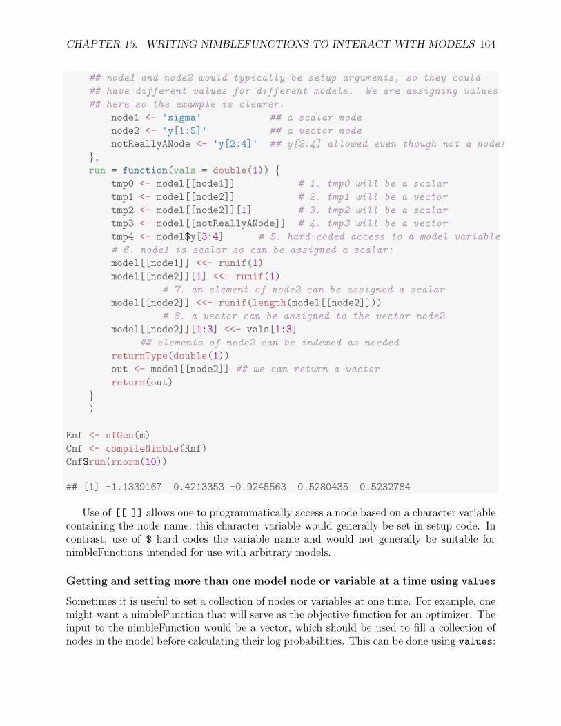
CHAPTER 15. WRITING NIMBLEFUNCTIONS TO INTERACT WITH MODELS 164
## node1 and node2 would typically be setup arguments, so they could
## have different values for different models. We are assigning values
## here so the example is clearer.
node1 <- 'sigma' ## a scalar node
node2 <- 'y[1:5]' ## a vector node
notReallyANode <- 'y[2:4]' ## y[2:4] allowed even though not a node!
},run = function(vals = double(1)) {
tmp0 <- model[[node1]] # 1. tmp0 will be a scalar
tmp1 <- model[[node2]] # 2. tmp1 will be a vector
tmp2 <- model[[node2]][1] # 3. tmp2 will be a scalar
tmp3 <- model[[notReallyANode]] # 4. tmp3 will be a vector
tmp4 <- model$y[3:4] # 5. hard-coded access to a model variable
# 6. node1 is scalar so can be assigned a scalar:
model[[node1]] <<- runif(1)
model[[node2]][1] <<- runif(1)
# 7. an element of node2 can be assigned a scalar
model[[node2]] <<- runif(length(model[[node2]]))
# 8. a vector can be assigned to the vector node2
model[[node2]][1:3] <<- vals[1:3]
## elements of node2 can be indexed as needed
returnType(double(1))
out <- model[[node2]] ## we can return a vector
return(out)
})
Rnf <- nfGen(m)
Cnf <- compileNimble(Rnf)
Cnf$run(rnorm(10))
## [1] -1.1339167 0.4213353 -0.9245563 0.5280435 0.5232784
Use of [[ ]] allows one to programmatically access a node based on a character variablecontaining the node name; this character variable would generally be set in setup code. Incontrast, use of $ hard codes the variable name and would not generally be suitable fornimbleFunctions intended for use with arbitrary models.
Getting and setting more than one model node or variable at a time using values
Sometimes it is useful to set a collection of nodes or variables at one time. For example, onemight want a nimbleFunction that will serve as the objective function for an optimizer. Theinput to the nimbleFunction would be a vector, which should be used to fill a collection ofnodes in the model before calculating their log probabilities. This can be done using values:
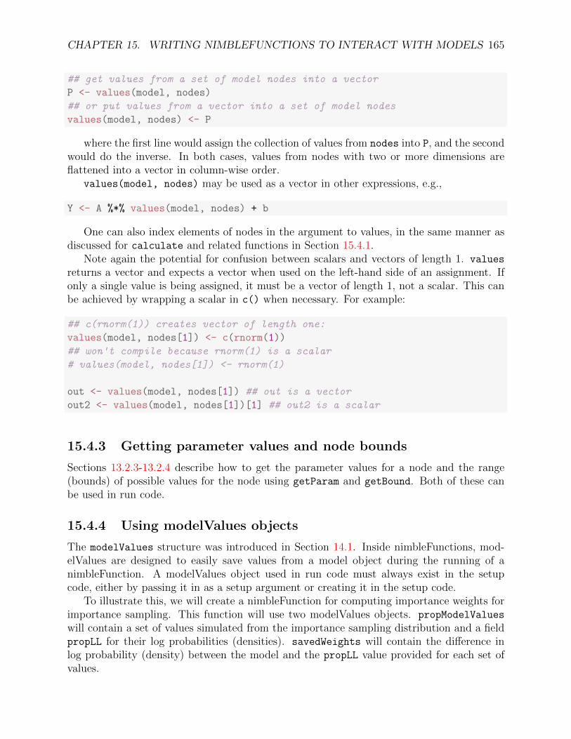
CHAPTER 15. WRITING NIMBLEFUNCTIONS TO INTERACT WITH MODELS 165
## get values from a set of model nodes into a vector
P <- values(model, nodes)
## or put values from a vector into a set of model nodes
values(model, nodes) <- P
where the first line would assign the collection of values from nodes into P, and the secondwould do the inverse. In both cases, values from nodes with two or more dimensions areflattened into a vector in column-wise order.
values(model, nodes) may be used as a vector in other expressions, e.g.,
Y <- A %*% values(model, nodes) + b
One can also index elements of nodes in the argument to values, in the same manner asdiscussed for calculate and related functions in Section 15.4.1.
Note again the potential for confusion between scalars and vectors of length 1. values
returns a vector and expects a vector when used on the left-hand side of an assignment. Ifonly a single value is being assigned, it must be a vector of length 1, not a scalar. This canbe achieved by wrapping a scalar in c() when necessary. For example:
## c(rnorm(1)) creates vector of length one:
values(model, nodes[1]) <- c(rnorm(1))
## won't compile because rnorm(1) is a scalar
# values(model, nodes[1]) <- rnorm(1)
out <- values(model, nodes[1]) ## out is a vector
out2 <- values(model, nodes[1])[1] ## out2 is a scalar
15.4.3 Getting parameter values and node bounds
Sections 13.2.3-13.2.4 describe how to get the parameter values for a node and the range(bounds) of possible values for the node using getParam and getBound. Both of these canbe used in run code.
15.4.4 Using modelValues objects
The modelValues structure was introduced in Section 14.1. Inside nimbleFunctions, mod-elValues are designed to easily save values from a model object during the running of animbleFunction. A modelValues object used in run code must always exist in the setupcode, either by passing it in as a setup argument or creating it in the setup code.
To illustrate this, we will create a nimbleFunction for computing importance weights forimportance sampling. This function will use two modelValues objects. propModelValues
will contain a set of values simulated from the importance sampling distribution and a fieldpropLL for their log probabilities (densities). savedWeights will contain the difference inlog probability (density) between the model and the propLL value provided for each set ofvalues.

CHAPTER 15. WRITING NIMBLEFUNCTIONS TO INTERACT WITH MODELS 166
## Accepting modelValues as a setup argument
swConf <- modelValuesConf(vars = "w",
types = "double",
sizes = 1)
setup = function(propModelValues, model, savedWeightsConf){## Building a modelValues in the setup function
savedWeights <- modelValues(conf = savedWeightsConf)
## List of nodes to be used in run function
modelNodes <- model$getNodeNames(stochOnly = TRUE,
includeData = FALSE)
}
The simplest way to pass values back and forth between models and modelValues insideof a nimbleFunction is with copy, which has the synonym nimCopy. See help(nimCopy) forargument details.
Alternatively, the values may be accessed via indexing of individual rows, using thenotation mv[var, i], where mv is a modelValues object, var is a variable name (not a nodename), and i is a row number. Likewise, the getsize and resize functions can be used asdiscussed in Section 14.1. However the function as.matrix does not work in run code.
Here is a run function to use these modelValues:
run = function(){## gets the number of rows of propSamples
m <- getsize(propModelValues)
## resized savedWeights to have the proper rows
resize(savedWeights, m)
for(i in 1:m){## Copying from propSamples to model.
## Node names of propSamples and model must match!
nimCopy(from = propModelValues, to = model, row = i,
nodes = modelNodes, logProb = FALSE)
## calculates the log likelihood of the model
targLL <- model$calculate()
## retreaves the saved log likelihood from the proposed model
propLL <- propModelValues["propLL",i][1]
## saves the importance weight for the i-th sample
savedWeights["w", i][1] <<- exp(targLL - propLL)
}## does not return anything
}
Once the nimbleFunction is built, the modelValues object can be accessed using $, whichis shown in more detail below. In fact, since modelValues, like most NIMBLE objects, are

CHAPTER 15. WRITING NIMBLEFUNCTIONS TO INTERACT WITH MODELS 167
reference class objects, one can get a reference to them before the function is executed andthen use that reference afterwards.
## simple model and modelValues for example use with code above
targetModelCode <- nimbleCode({x ~ dnorm(0,1)
for(i in 1:4)
y[i] ~ dnorm(0,1)
})
## code for proposal model
propModelCode <- nimbleCode({x ~ dnorm(0,2)
for(i in 1:4)
y[i] ~ dnorm(0,2)
})
## creating the models
targetModel = nimbleModel(targetModelCode, check = FALSE)
propModel = nimbleModel(propModelCode, check = FALSE)
cTargetModel = compileNimble(targetModel)
cPropModel = compileNimble(propModel)
sampleMVConf = modelValuesConf(vars = c("x", "y", "propLL"),
types = c("double", "double", "double"),
sizes = list(x = 1, y = 4, propLL = 1) )
sampleMV <- modelValues(sampleMVConf)
## nimbleFunction for generating proposal sample
PropSamp_Gen <- nimbleFunction(
setup = function(mv, propModel){nodeNames <- propModel$getNodeNames()
},run = function(m = integer() ){
resize(mv, m)
for(i in 1:m){propModel$simulate()
nimCopy(from = propModel, to = mv, nodes = nodeNames, row = i)
mv["propLL", i][1] <<- propModel$calculate()
}})

CHAPTER 15. WRITING NIMBLEFUNCTIONS TO INTERACT WITH MODELS 168
## nimbleFunction for calculating importance weights
## uses setup and run functions as defined in previous code chunk
impWeights_Gen <- nimbleFunction(setup = setup,
run = run)
## making instances of nimbleFunctions
## note that both functions share the same modelValues object
RPropSamp <- PropSamp_Gen(sampleMV, propModel)
RImpWeights <- impWeights_Gen(sampleMV, targetModel, swConf)
## compiling
CPropSamp <- compileNimble(RPropSamp, project = propModel)
CImpWeights <- compileNimble(RImpWeights, project = targetModel)
## generating and saving proposal sample of size 10
CPropSamp$run(10)
## NULL
## calculating the importance weights and saving to mv
CImpWeights$run()
## NULL
## retrieving the modelValues objects
## extracted objects are C-based modelValues objects
savedPropSamp_1 = CImpWeights$propModelValues
savedPropSamp_2 = CPropSamp$mv
# Subtle note: savedPropSamp_1 and savedPropSamp_2
# both provide interface to the same compiled modelValues objects!
# This is because they were both built from sampleMV.
savedPropSamp_1["x",1]
## [1] 0.5615461
savedPropSamp_2["x",1]
## [1] 0.5615461
savedPropSamp_1["x",1] <- 0 ## example of directly setting a value
savedPropSamp_2["x",1]

CHAPTER 15. WRITING NIMBLEFUNCTIONS TO INTERACT WITH MODELS 169
## [1] 0
## viewing the saved importance weights
savedWeights <- CImpWeights$savedWeights
unlist(savedWeights[["w"]])
## [1] 0.3159913 0.3114850 1.3655582 0.3969088 41.3934032
## [6] 0.2732388 0.7972150 1.5456142 0.4199902 1.8547728
## viewing first 3 rows -- note that savedPropSsamp_1["x", 1] was altered
as.matrix(savedPropSamp_1)[1:3, ]
## propLL[1] x[1] y[1] y[2] y[3]
## [1,] -4.023479 0.0000000 -0.4634227 -0.4790402 0.1299793
## [2,] -3.994752 -0.2773491 -0.4730179 -0.7142721 -0.5309174
## [3,] -6.950687 -0.8243472 0.4887699 -1.4541917 -0.1090178
## y[4]
## [1,] 0.6206335
## [2,] -0.2005022
## [3,] -1.0216946
Importance sampling could also be written using simple vectors for the weights, but weillustrated putting them in a modelValues object along with model variables.
15.4.5 Using model variables and modelValues in expressions
Each way of accessing a variable, node, or modelValues can be used amidst mathematicalexpressions, including with indexing, or passed to another nimbleFunction as an argument.For example, the following two statements would be valid:
model[["x[2:8, ]"]][2:4, 1:3] %*% Z
if Z is a vector or matrix, and
C[6:10] <- mv[v, i][1:5, k] + B
if B is a vector or matrix.The NIMBLE language allows scalars, but models defined from BUGS code are never
created as purely scalar nodes. Instead, a single node such as defined by z ∼ dnorm(0,
1) is implemented as a vector of length 1, similar to R. When using z via model$z ormodel[["z"]], NIMBLE will try to do the right thing by treating this as a scalar. In theevent of problems5, a more explicit way to access z is model$z[1] or model[["z"]][1].
5Please tell us!

CHAPTER 15. WRITING NIMBLEFUNCTIONS TO INTERACT WITH MODELS 170
15.4.6 Including other methods in a nimbleFunction
Other methods can be included with the methods argument to nimbleFunction. Thesemethods can use the objects created in setup code in just the same ways as the run function.In fact, the run function is just a default main method name. Any method can then callanother method.
methodsDemo <- nimbleFunction(
setup = function() {sharedValue <- 1},run = function(x = double(1)) {
print("sharedValues = ", sharedValue, "\n")increment()
print("sharedValues = ", sharedValue, "\n")A <- times(5)
return(A * x)
returnType(double(1))
},methods = list(
increment = function() {sharedValue <<- sharedValue + 1
},times = function(factor = double()) {
return(factor * sharedValue)
returnType(double())
}))
methodsDemo1 <- methodsDemo()
methodsDemo1$run(1:10)
## sharedValues = 1
##
## sharedValues = 2
## [1] 10 20 30 40 50 60 70 80 90 100
methodsDemo1$sharedValue <- 1
CmethodsDemo1 <- compileNimble(methodsDemo1)
CmethodsDemo1$run(1:10)
## sharedValues = 1
##
## sharedValues = 2
## [1] 10 20 30 40 50 60 70 80 90 100

CHAPTER 15. WRITING NIMBLEFUNCTIONS TO INTERACT WITH MODELS 171
15.4.7 Using other nimbleFunctions
One nimbleFunction can use another nimbleFunction that was passed to it as a setup argu-ment or was created in the setup function. This can be an effective way to program. Whena nimbleFunction needs to access a setup variable or method of another nimbleFunction, use$.
usePreviousDemo <- nimbleFunction(
setup = function(initialSharedValue) {myMethodsDemo <- methodsDemo()
},run = function(x = double(1)) {
myMethodsDemo$sharedValue <<- initialSharedValue
print(myMethodsDemo$sharedValue)
A <- myMethodsDemo$run(x[1:5])
print(A)
B <- myMethodsDemo$times(10)
return(B)
returnType(double())
})
usePreviousDemo1 <- usePreviousDemo(2)
usePreviousDemo1$run(1:10)
## 2
## sharedValues = 2
##
## sharedValues = 3
##
## 15 30 45 60 75
## [1] 30
CusePreviousDemo1 <- compileNimble(usePreviousDemo1)
CusePreviousDemo1$run(1:10)
## 2
## sharedValues = 2
##
## sharedValues = 3
##
## 15
## 30
## 45
## 60
## 75
## [1] 30

CHAPTER 15. WRITING NIMBLEFUNCTIONS TO INTERACT WITH MODELS 172
15.4.8 Virtual nimbleFunctions and nimbleFunctionLists
Often it is useful for one nimbleFunction to have a list of other nimbleFunctions, all of whosemethods have the same arguments and return types. For example, NIMBLE’s MCMC enginecontains a list of samplers that are each nimbleFunctions.
To make such a list, NIMBLE provides a way to declare the arguments and returntypes of methods: virtual nimbleFunctions created by nimbleFunctionVirtual. OthernimbleFunctions can inherit from virtual nimbleFunctions, which in R is called “containing”them. Readers familiar with object oriented programming will recognize this as a simpleclass inheritance system. In Version 0.6-11 it is limited to simple, single-level inheritance.
Here is how it works:
baseClass <- nimbleFunctionVirtual(
run = function(x = double(1)) {returnType(double())},methods = list(
foo = function() {returnType(double())}))
derived1 <- nimbleFunction(
contains = baseClass,
setup = function(){},run = function(x = double(1)) {
print("run 1")
return(sum(x))
returnType(double())
},methods = list(
foo = function() {print("foo 1")
return(rnorm(1, 0, 1))
returnType(double())
}))
derived2 <- nimbleFunction(
contains = baseClass,
setup = function(){},run = function(x = double(1)) {
print("run 2")
return(prod(x))
returnType(double())
},methods = list(
foo = function() {print("foo 2")
return(runif(1, 100, 200))

CHAPTER 15. WRITING NIMBLEFUNCTIONS TO INTERACT WITH MODELS 173
returnType(double())
}))
useThem <- nimbleFunction(
setup = function() {nfl <- nimbleFunctionList(baseClass)
nfl[[1]] <- derived1()
nfl[[2]] <- derived2()
},run = function(x = double(1)) {
for(i in seq_along(nfl)) {print( nfl[[i]]$run(x) )
print( nfl[[i]]$foo() )
}})
useThem1 <- useThem()
set.seed(1)
useThem1$run(1:5)
## run 1
## 15
## foo 1
## -0.6264538
## run 2
## 120
## foo 2
## 157.2853
CuseThem1 <- compileNimble(useThem1)
set.seed(1)
CuseThem1$run(1:5)
## run 1
## 15
## foo 1
## -0.626454
## run 2
## 120
## foo 2
## 157.285
## NULL
One can also use seq along with nimbleFunctionLists (and only with nimbleFunction-

CHAPTER 15. WRITING NIMBLEFUNCTIONS TO INTERACT WITH MODELS 174
Lists). As in R, seq along(myFunList) is equivalent to 1:length(myFunList) if the lengthof myFunList is greater than zero. It is an empty sequence if the length is zero.
Virtual nimbleFunctions cannot define setup values to be inherited.
15.4.9 Character objects
NIMBLE provides limited uses of character objects in run code. Character vectors createdin setup code will be available in run code, but the only thing you can really do with themis include them in a print or stop statement.
Note that character vectors of model node and variable names are processed duringcompilation. For example, in model[[node]], node may be a character object, and theNIMBLE compiler processes this differently than print("The node name was ", node).In the former, the NIMBLE compiler sets up a C++ pointer directly to the node in themodel, so that the character content of node is never needed in C++. In the latter, node isused as a C++ string and therefore is needed in C++.
15.4.10 User-defined data structures
Before the introduction of nimbleLists in Version 0.6-4, NIMBLE did not explicitly haveuser-defined data structures. An alternative way to create a data structure in NIMBLE isto use nimbleFunctions to achieve a similar effect. To do so, one can define setup code withwhatever variables are wanted and ensure they are compiled using setupOutputs. Here isan example:
dataNF <- nimbleFunction(
setup = function() {X <- 1
Y <- as.numeric(c(1, 2))
Z <- matrix(as.numeric(1:4), nrow = 2)
setupOutputs(X, Y, Z)
})
useDataNF <- nimbleFunction(
setup = function(myDataNF) {},run = function(newX = double(), newY = double(1), newZ = double(2)) {
myDataNF$X <<- newX
myDataNF$Y <<- newY
myDataNF$Z <<- newZ
})
myDataNF <- dataNF()
myUseDataNF <- useDataNF(myDataNF)
myUseDataNF$run(as.numeric(100), as.numeric(100:110),
matrix(as.numeric(101:120), nrow = 2))
myDataNF$X

CHAPTER 15. WRITING NIMBLEFUNCTIONS TO INTERACT WITH MODELS 175
## [1] 100
myDataNF$Y
## [1] 100 101 102 103 104 105 106 107 108 109 110
myDataNF$Z
## [,1] [,2] [,3] [,4] [,5] [,6] [,7] [,8] [,9] [,10]
## [1,] 101 103 105 107 109 111 113 115 117 119
## [2,] 102 104 106 108 110 112 114 116 118 120
myUseDataNF$myDataNF$X
## [1] 100
nimbleOptions(buildInterfacesForCompiledNestedNimbleFunctions = TRUE)
CmyUseDataNF <- compileNimble(myUseDataNF)
CmyUseDataNF$run(-100, -(100:110), matrix(-(101:120), nrow = 2))
## NULL
CmyDataNF <- CmyUseDataNF$myDataNF
CmyDataNF$X
## [1] -100
CmyDataNF$Y
## [1] -100 -101 -102 -103 -104 -105 -106 -107 -108 -109 -110
CmyDataNF$Z
## [,1] [,2] [,3] [,4] [,5] [,6] [,7] [,8] [,9] [,10]
## [1,] -101 -103 -105 -107 -109 -111 -113 -115 -117 -119
## [2,] -102 -104 -106 -108 -110 -112 -114 -116 -118 -120
You’ll notice that:
• After execution of the compiled function, access to the X, Y, and Z is the same as forthe uncompiled case. This occurs because CmyUseDataNF is an interface to the com-piled version of myUseDataNF, and it provides access to member objects and functions.In this case, one member object is myDataNF, which is an interface to the compiledversion of myUseDataNF$myDataNF, which in turn provides access to X, Y, and Z. Toreduce memory use, NIMBLE defaults to not providing full interfaces to nested nim-bleFunctions like myUseDataNF$myDataNF. In this example we made it provide full

CHAPTER 15. WRITING NIMBLEFUNCTIONS TO INTERACT WITH MODELS 176
interfaces by setting the buildInterfacesForCompiledNestedNimbleFunctions op-tion via nimbleOptions to TRUE. If we had left that option FALSE (its default value),we could still get to the values of interest using
valueInCompiledNimbleFunction(CmyDataNF, 'X')
• We need to take care that at the time of compilation, the X, Y and Z values containdoubles via as.numeric so that they are not compiled as integer objects.• The myDataNF could be created in the setup code. We just provided it as a setup
argument to illustrate that option.
15.5 Example: writing user-defined samplers to ex-
tend NIMBLE’s MCMC engine
One important use of nimbleFunctions is to write additional samplers that can be used inNIMBLE’s MCMC engine. This allows a user to write a custom sampler for one or morenodes in a model, as well as for programmers to provide general samplers for use in additionto the library of samplers provided with NIMBLE.
The following code illustrates how a NIMBLE developer would implement and use aMetropolis-Hastings random walk sampler with fixed proposal standard deviation.
my_RW <- nimbleFunction(
contains = sampler_BASE,
setup = function(model, mvSaved, target, control) {## proposal standard deviation
scale <- if(!is.null(control$scale)) control$scale else 1
calcNodes <- model$getDependencies(target)
},
run = function() {## initial model logProb
model_lp_initial <- getLogProb(model, calcNodes)
## generate proposal
proposal <- rnorm(1, model[[target]], scale)
## store proposal into model
model[[target]] <<- proposal
## proposal model logProb
model_lp_proposed <- calculate(model, calcNodes)
## log-Metropolis-Hastings ratio
log_MH_ratio <- model_lp_proposed - model_lp_initial

CHAPTER 15. WRITING NIMBLEFUNCTIONS TO INTERACT WITH MODELS 177
## Metropolis-Hastings step: determine whether or
## not to accept the newly proposed value
u <- runif(1, 0, 1)
if(u < exp(log_MH_ratio)) jump <- TRUE
else jump <- FALSE
## keep the model and mvSaved objects consistent
if(jump) copy(from = model, to = mvSaved, row = 1,
nodes = calcNodes, logProb = TRUE)
else copy(from = mvSaved, to = model, row = 1,
nodes = calcNodes, logProb = TRUE)
},
methods = list( reset = function () {} )
)
The name of this sampler function, for the purposes of using it in an MCMC algorithm,is my RW. Thus, this sampler can be added to an exisiting MCMC configuration object confusing:
mcmcConf$addSampler(target = 'x', type = 'my_RW',
control = list(scale = 0.1))
To be used within the MCMC engine, sampler functions definitions must adhere exactlyto the following:
• The nimbleFunction must include the contains statement contains = sampler BASE.• The setup function must have the four arguments model, mvSaved, target, control,
in that order.• The run function must accept no arguments, and have no return value. Further, after
execution it must leave the mvSaved modelValues object as an up-to-date copy of thevalues and logProb values in the model object.• The nimbleFunction must have a member method called reset, which takes no argu-
ments and has no return value.
The purpose of the setup function is generally two-fold. First, to extract control pa-rameters from the control list; in the example, the proposal standard deviation scale. Itis good practice to specify default values for any control parameters that are not providedin the control argument, as done in the example. Second, to generate any sets of nodesneeded in the run function. In many sampling algorithms, as here, calcNodes is used torepresent the target node(s) and dependencies up to the first layer of stochastic nodes, as thisis precisely what is required for calculating the Metropolis-Hastings acceptance probability.These probability calculations are done using model$calculate(calcNodes).
In the run function, the mvSaved modelValues object is kept up-to-date with the currentstate of the model, depending on whether the proposed changed was accepted. This is doneusing the copy function, to copy values between the model and mvSaved objects.

CHAPTER 15. WRITING NIMBLEFUNCTIONS TO INTERACT WITH MODELS 178
15.6 Copying nimbleFunctions (and NIMBLE models)
NIMBLE relies heavily on R’s reference class system. When models, modelValues, and nim-bleFunctions with setup code are created, NIMBLE generates a new, customized referenceclass definition for each. As a result, objects of these types are passed by reference and hencemodified in place by most NIMBLE operations. This is necessary to avoid a great deal ofcopying and returning and having to reassign large objects, both in processing models andnimbleFunctions and in running algorithms.
One cannot generally copy NIMBLE models or nimbleFunctions (specializations or gener-ators) in a safe fashion, because of the references to other objects embedded within NIMBLEobjects. However, the model member function newModel will create a new copy of the modelfrom the same model definition (Section 6.1.3). This new model can then be used with newlyinstantiated nimbleFunctions.
The reliable way to create new copies of nimbleFunctions is to re-run the R functioncalled nimbleFunction and record the result in a new object. For example, say you have animbleFunction called foo and 1000 instances of foo are compiled as part of an algorithmrelated to a model called model1. If you then need to use foo in an algorithm for anothermodel, model2, doing so may work without any problems. However, there are cases wherethe NIMBLE compiler will tell you during compilation that the second set of foo instancescannot be built from the previous compiled version. A solution is to re-define foo from thebeginning – i.e. call nimbleFunction again – and then proceed with building and compilingthe algorithm for model2.
15.7 Debugging nimbleFunctions
One of the main reasons that NIMBLE provides an R (uncompiled) version of each nimble-Function is for debugging. One can call debug on nimbleFunction methods (in particularthe main run method, e.g., debug(mynf$run) and then step through the code in R using R’sdebugger. One can also insert browser calls into run code and then run the nimbleFunctionfrom R.
In contrast, directly debugging a compiled nimbleFunction is difficult, although thosefamiliar with running R through a debugger and accessing the underlying C code maybe able to operate similarly with NIMBLE code. We often resort to using print state-ments for debugging compiled code. Expert users fluent in C++ may also try settingnimbleOptions(pauseAfterWritingFiles = TRUE) and adding debugging code into thegenerated C++ files.
15.8 Timing nimbleFunctions with run.time
If your nimbleFunctions are correct but slow to run, you can use benchmarking tools tolook for bottlenecks and to compare different implementations. If your functions are verylong-running (say 1ms or more), then standard R benchmarking tools may suffice, e.g. themicrobenchmark package

CHAPTER 15. WRITING NIMBLEFUNCTIONS TO INTERACT WITH MODELS 179
library(microbenchmark)
microbenchmark(myCompiledFunVersion1(1.234),
myCompiledFunVersion2(1.234)) # Beware R <--> C++ overhead!
If your nimbleFunctions are very fast, say under 1ms, then microbenchmark will be in-acurate due to R-to-C++ conversion overhead (that won’t happen in your actual functions).To get timing information in C++, NIMBLE provides a run.time function that avoids theR-to-C++ overhead.
myMicrobenchmark <- compileNimble(nimbleFunction(
run = function(iters = integer(0)){time1 <- run.time({
for (t in 1:iters) myCompiledFunVersion1(1.234)
})time2 <- run.time({
for (t in 1:iters) myCompiledFunVersion2(1.234)
})return(c(time1, time2))
returnType(double(1))
}))print(myMicroBenchmark(100000))
15.9 Reducing memory usage
NIMBLE can create a lot of objects in its processing, and some of them use R features suchas reference classes that are heavy in memory usage. We have noticed that building largemodels can use lots of memory. To help alleviate this, we provide two options, which can becontrolled via nimbleOptions.
As noted above, the option buildInterfacesForCompiledNestedNimbleFunctions de-faults to FALSE, which means NIMBLE will not build full interfaces to compiled nimble-Functions that ony appear within other nimbleFunctions. If you want access to all suchnimbleFunctions, use the option buildInterfacesForCompiledNestedNimbleFunctions =
TRUE.The option clearNimbleFunctionsAfterCompiling is more drastic, and it is experimen-
tal, so “buyer beware”. This will clear much of the contents of an uncompiled nimbleFunctionobject after it has been compiled in an effort to free some memory. We expect to be ableto keep making NIMBLE more efficient – faster execution and lower memory use – in thefuture.

Bibliography
[1] Andrieu, C., A. Doucet, and R. Holenstein (2010). Particle Markov chain Monte Carlomethods. Journal of the Royal Statistical Society: Series B (Statistical Methodology) 72 (3),269–342.
[2] Banerjee, S., B. Carlin, and A. Gelfand (2015). Hierarchical Modeling and Analysis forSpatial Data (2 ed.). Boca Raton: Chapman & Hall.
[3] Blackwell, D. and J. MacQueen (1973). Ferguson distributions via Polya urn schemes.The Annals of Statistics 1, 353–355.
[4] Escobar, M. D. (1994). Estimating normal means with a Dirichlet process prior. Journalof the American Statistical Association 89, 268–277.
[5] Escobar, M. D. and M. West (1995). Bayesian density estimation and inference usingmixtures. Journal of the American Statistical Association 90, 577–588.
[6] Ferguson, T. S. (1973). A Bayesian analysis of some nonparametric problems. Annals ofStatistics 1, 209–230.
[7] Ferguson, T. S. (1974). Prior distribution on the spaces of probability measures. Annalsof Statistics 2, 615–629.
[8] George, E., U. Makov, and A. Smith (1993). Conjugate likelihood distributions. Scandi-navian Journal of Statistics 20 (2), 147–156.
[9] Ishwaran, H. and L. F. James (2001). Gibbs sampling methods for stick-breaking priors.Journal of the American Statistical Association 96 (453), 161–173.
[10] Ishwaran, H. and L. F. James (2002). Approximate Dirichlet process computing infinite normal mixtures: smoothing and prior information. Journal of Computational andGraphical Statistics 11, 508–532.
[11] Lo, A. Y. (1984). On a class of Bayesian nonparametric estimates I: Density estimates.The Annals of Statistics 12, 351–357.
[12] Lunn, D., D. Spiegelhalter, A. Thomas, and N. Best (2009). The BUGS project: Evo-lution, critique and future directions. Statistics in Medicine 28 (25), 3049–3067.
[13] Neal, R. (2000). Markov chain sampling methods for Dirichlet process mixture models.Journal of Computational and Graphical Statistics 9, 249–265.
180

BIBLIOGRAPHY 181
[14] Neal, R. M. (2003). Slice sampling. The Annals of Statistics 31 (3), 705–741.
[15] Paciorek, C. (2009). Understanding intrinsic Gaussian Markov random field spatialmodels, including intrinsic conditional autoregressive models. Technical report, Universityof California, Berkeley.
[16] Roberts, G. O. and S. K. Sahu (1997). Updating schemes, correlation structure, blockingand parameterization for the Gibbs sampler. Journal of the Royal Statistical Society:Series B (Statistical Methodology) 59 (2), 291317.
[17] Rue, H. and L. Held (2005). Gaussian Markov Random Fields: Theory and Applications.Boca Raton: Chapman & Hall.
[18] Sethuraman, J. (1994). A constructive definition of Dirichlet prior. Statistica Sinica 2,639–650.
[19] Watanabe, S. (2010). Asymptotic equivalence of Bayes cross validation and widelyapplicable information criterion in singular learning theory. Journal of Machine LearningResearch 11 (Dec), 3571–3594.