Newton’s Method

Ryan TibshiraniConvex Optimization 10-725/36-725

1

Last time: dual correspondences

Given a function f : Rn → R, we define its conjugate f∗ : Rn → R,

f∗(y) = maxx

yTx− f(x)

Properties and examples:

• Conjugate f∗ is always convex (regardless of convexity of f)

• When f is a quadratic in Q � 0, f∗ is a quadratic in Q−1

• When f is a norm, f∗ is the indicator of the dual norm unitball

• When f is closed and convex, x ∈ ∂f∗(y) ⇐⇒ y ∈ ∂f(x)

Relationship to duality:

Primal : minx

f(x) + g(x)

Dual : maxu−f∗(u)− g∗(−u)

2

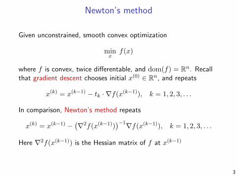
Newton’s method

Given unconstrained, smooth convex optimization

minx

f(x)

where f is convex, twice differentable, and dom(f) = Rn. Recallthat gradient descent chooses initial x(0) ∈ Rn, and repeats

x(k) = x(k−1) − tk · ∇f(x(k−1)), k = 1, 2, 3, . . .

In comparison, Newton’s method repeats

x(k) = x(k−1) −(∇2f(x(k−1))

)−1∇f(x(k−1)), k = 1, 2, 3, . . .

Here ∇2f(x(k−1)) is the Hessian matrix of f at x(k−1)

3

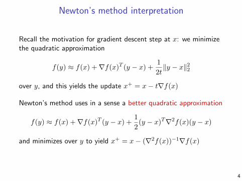
Newton’s method interpretation

Recall the motivation for gradient descent step at x: we minimizethe quadratic approximation

f(y) ≈ f(x) +∇f(x)T (y − x) +1

2t‖y − x‖22

over y, and this yields the update x+ = x− t∇f(x)

Newton’s method uses in a sense a better quadratic approximation

f(y) ≈ f(x) +∇f(x)T (y − x) +1

2(y − x)T∇2f(x)(y − x)

and minimizes over y to yield x+ = x− (∇2f(x))−1∇f(x)

4

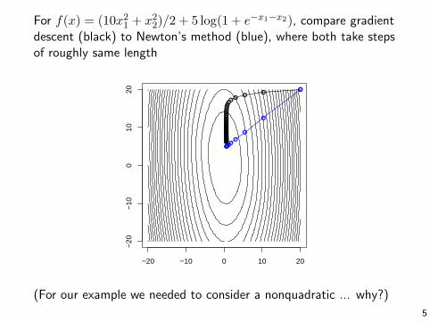
For f(x) = (10x21 + x22)/2 + 5 log(1 + e−x1−x2), compare gradientdescent (black) to Newton’s method (blue), where both take stepsof roughly same length

−20 −10 0 10 20

−20

−10

010

20 ●●

●●

●●●●●●●●●●●●●●●●●●●●●●●●●●●●●●●●●●●●●●●●●●●●●●

●

●

●

●●●●●●●

(For our example we needed to consider a nonquadratic ... why?)

5

Outline

Today:

• Interpretations and properties

• Backtracking line search

• Convergence analysis

• Equality-constrained Newton

• Quasi-Newton methods

6

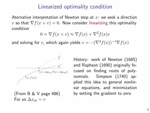
Linearized optimality condition

Aternative interpretation of Newton step at x: we seek a directionv so that ∇f(x+ v) = 0. Now consider linearizing this optimalitycondition

0 = ∇f(x+ v) ≈ ∇f(x) +∇2f(x)v

and solving for v, which again yields v = −(∇2f(x))−1∇f(x)486 9 Unconstrained minimization

f ′

!f ′

(x, f ′(x))

(x + ∆xnt, f′(x + ∆xnt))

Figure 9.18 The solid curve is the derivative f ′ of the function f shown in

figure 9.16. !f ′ is the linear approximation of f ′ at x. The Newton step ∆xnt

is the difference between the root of !f ′ and the point x.

the zero-crossing of the derivative f ′, which is monotonically increasing since f isconvex. Given our current approximation x of the solution, we form a first-orderTaylor approximation of f ′ at x. The zero-crossing of this affine approximation isthen x + ∆xnt. This interpretation is illustrated in figure 9.18.

Affine invariance of the Newton step

An important feature of the Newton step is that it is independent of linear (oraffine) changes of coordinates. Suppose T ∈ Rn×n is nonsingular, and definef̄(y) = f(Ty). Then we have

∇f̄(y) = TT ∇f(x), ∇2f̄(y) = TT ∇2f(x)T,

where x = Ty. The Newton step for f̄ at y is therefore

∆ynt = −"TT ∇2f(x)T

#−1 "TT ∇f(x)

#

= −T−1∇2f(x)−1∇f(x)

= T−1∆xnt,

where ∆xnt is the Newton step for f at x. Hence the Newton steps of f and f̄ arerelated by the same linear transformation, and

x + ∆xnt = T (y + ∆ynt).

The Newton decrement

The quantity

λ(x) ="∇f(x)T ∇2f(x)−1∇f(x)

#1/2

is called the Newton decrement at x. We will see that the Newton decrementplays an important role in the analysis of Newton’s method, and is also useful

(From B & V page 486)For us ∆xnt = v

History: work of Newton (1685)and Raphson (1690) originally fo-cused on finding roots of poly-nomials. Simpson (1740) ap-plied this idea to general nonlin-ear equations, and minimizationby setting the gradient to zero

7

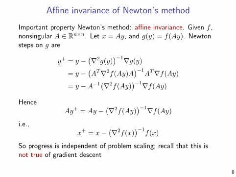
Affine invariance of Newton’s method

Important property Newton’s method: affine invariance. Given f ,nonsingular A ∈ Rn×n. Let x = Ay, and g(y) = f(Ay). Newtonsteps on g are

y+ = y −(∇2g(y)

)−1∇g(y)

= y −(AT∇2f(Ay)A

)−1AT∇f(Ay)

= y −A−1(∇2f(Ay)

)−1∇f(Ay)

HenceAy+ = Ay −

(∇2f(Ay)

)−1∇f(Ay)

i.e.,x+ = x−

(∇2f(x)

)−1f(x)

So progress is independent of problem scaling; recall that this isnot true of gradient descent

8

Newton decrement

At a point x, we define the Newton decrement as

λ(x) =(∇f(x)T

(∇2f(x)

)−1∇f(x))1/2

This relates to the difference between f(x) and the minimum of itsquadratic approximation:

f(x)−miny

(f(x) +∇f(x)T (y − x) +

1

2(y − x)T∇2f(x)(y − x)

)

= f(x)−(f(x)− 1

2∇f(x)T

(∇2f(x)

)−1∇f(x))

=1

2λ(x)2

Therefore can think of λ2(x)/2 as an approximate bound on thesuboptimality gap f(x)− f?

9

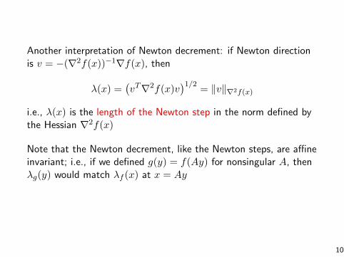
Another interpretation of Newton decrement: if Newton directionis v = −(∇2f(x))−1∇f(x), then

λ(x) =(vT∇2f(x)v

)1/2= ‖v‖∇2f(x)

i.e., λ(x) is the length of the Newton step in the norm defined bythe Hessian ∇2f(x)

Note that the Newton decrement, like the Newton steps, are affineinvariant; i.e., if we defined g(y) = f(Ay) for nonsingular A, thenλg(y) would match λf (x) at x = Ay

10

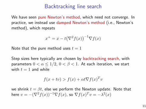
Backtracking line search

We have seen pure Newton’s method, which need not converge. Inpractice, we instead use damped Newton’s method (i.e., Newton’smethod), which repeats

x+ = x− t(∇2f(x)

)−1∇f(x)

Note that the pure method uses t = 1

Step sizes here typically are chosen by backtracking search, withparameters 0 < α ≤ 1/2, 0 < β < 1. At each iteration, we startwith t = 1 and while

f(x+ tv) > f(x) + αt∇f(x)T v

we shrink t = βt, else we perform the Newton update. Note thathere v = −(∇2f(x))−1∇f(x), so ∇f(x)T v = −λ2(x)

11

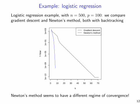
Example: logistic regression

Logistic regression example, with n = 500, p = 100: we comparegradient descent and Newton’s method, both with backtracking

0 10 20 30 40 50 60 70

1e−

131e

−09

1e−

051e

−01

1e+

03

k

f−fs

tar

Gradient descentNewton's method

Newton’s method seems to have a different regime of convergence!12

Convergence analysis

Assume that f convex, twice differentiable, having dom(f) = Rn,and additionally

• ∇f is Lipschitz with parameter L

• f is strongly convex with parameter m

• ∇2f is Lipschitz with parameter M

Theorem: Newton’s method with backtracking line search sat-isfies the following two-stage convergence bounds

f(x(k))− f? ≤

(f(x(0))− f?)− γk if k ≤ k02m3

M2

(1

2

)2k−k0+1

if k > k0

Here γ = αβ2η2m/L2, η = min{1, 3(1− 2α)}m2/M , and k0 isthe number of steps until ‖∇f(x(k0+1))‖2 < η

13

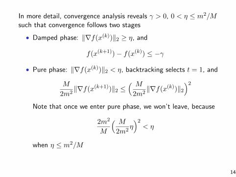
In more detail, convergence analysis reveals γ > 0, 0 < η ≤ m2/Msuch that convergence follows two stages

• Damped phase: ‖∇f(x(k))‖2 ≥ η, and

f(x(k+1))− f(x(k)) ≤ −γ

• Pure phase: ‖∇f(x(k))‖2 < η, backtracking selects t = 1, and

M

2m2‖∇f(x(k+1))‖2 ≤

( M

2m2‖∇f(x(k))‖2

)2

Note that once we enter pure phase, we won’t leave, because

2m2

M

( M

2m2η)2

< η

when η ≤ m2/M

14

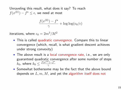
Unraveling this result, what does it say? To reachf(x(k))− f? ≤ ε, we need at most

f(x(0))− f?γ

+ log log(ε0/ε)

iterations, where ε0 = 2m3/M2

• This is called quadratic convergence. Compare this to linearconvergence (which, recall, is what gradient descent achievesunder strong convexity)

• The above result is a local convergence rate, i.e., we are onlyguaranteed quadratic convergence after some number of stepsk0, where k0 ≤ f(x(0))−f?

γ

• Somewhat bothersome may be the fact that the above bounddepends on L,m,M , and yet the algorithm itself does not

15

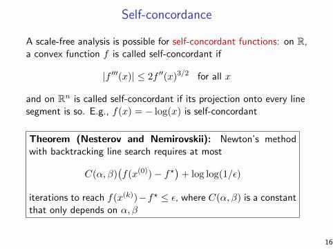
Self-concordance

A scale-free analysis is possible for self-concordant functions: on R,a convex function f is called self-concordant if

|f ′′′(x)| ≤ 2f ′′(x)3/2 for all x

and on Rn is called self-concordant if its projection onto every linesegment is so. E.g., f(x) = − log(x) is self-concordant

Theorem (Nesterov and Nemirovskii): Newton’s methodwith backtracking line search requires at most

C(α, β)(f(x(0))− f?

)+ log log(1/ε)

iterations to reach f(x(k))−f? ≤ ε, where C(α, β) is a constantthat only depends on α, β

16

Comparison to first-order methods

At a high-level:

• Memory: each iteration of Newton’s method requires O(n2)storage (n× n Hessian); each gradient iteration requires O(n)storage (n-dimensional gradient)

• Computation: each Newton iteration requires O(n3) flops(solving a dense n× n linear system); each gradient iterationrequires O(n) flops (scaling/adding n-dimensional vectors)

• Backtracking: backtracking line search has roughly the samecost, both use O(n) flops per inner backtracking step

• Conditioning: Newton’s method is not affected by a problem’sconditioning, but gradient descent can seriously degrade

• Fragility: Newton’s method may be empirically more sensitiveto bugs/numerical errors, gradient descent is more robust

17

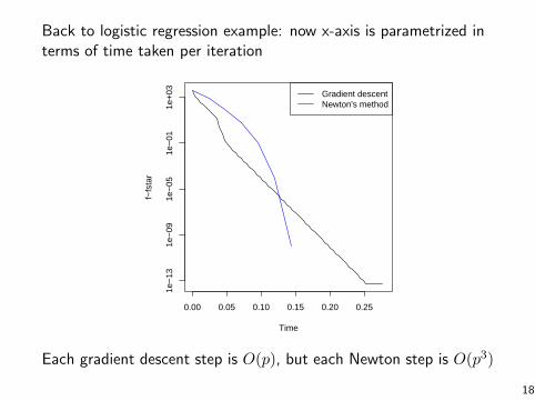
Back to logistic regression example: now x-axis is parametrized interms of time taken per iteration

0.00 0.05 0.10 0.15 0.20 0.25

1e−

131e

−09

1e−

051e

−01

1e+

03

Time

f−fs

tar

Gradient descentNewton's method

Each gradient descent step is O(p), but each Newton step is O(p3)

18

Sparse, structured problems

When the inner linear systems (in Hessian) can be solved efficientlyand reliably, Newton’s method can strive

E.g., if ∇2f(x) is sparse and structured for all x, say banded, thenboth memory and computation are O(n) with Newton iterations

What functions admit a structured Hessian? Two examples:

• If g(β) = f(Xβ), then ∇2g(β) = XT∇2f(Xβ)X. Hence ifX is a structured predictor matrix and ∇2f is diagonal, then∇2g is structured

• If we seek to minimize f(β) + g(Dβ), where ∇2f is diagonal,g is not smooth, and D is a structured penalty matrix, thenthe Lagrange dual function is −f∗(−DTu)− g∗(−u). Often−D∇2f∗(−DTu)DT can be structured

19

Equality-constrained Newton’s method

Consider now a problem with equality constraints, as in

minx

f(x) subject to Ax = b

Several options:

• Eliminating equality constraints: write x = Fy + x0, where Fspans null space of A, and Ax0 = b. Solve in terms of y

• Deriving the dual: can check that the Lagrange dual functionis −f∗(−AT v)− bT v, and strong duality holds. With luck, wecan express x? in terms of v?

• Equality-constrained Newton: in many cases, this is the moststraightforward option

20

In equality-constrained Newton’s method, we start with x(0) suchthat Ax(0) = b. Then we repeat the updates

x+ = x+ tv, where

v = argminAz=0

∇f(x)T (z − x) +1

2(z − x)T∇2f(x)(z − x)

This keeps x+ in feasible set, since Ax+ = Ax+ tAv = b+ 0 = b

Furthermore, v is the solution to minimizing a quadratic subject toequality constraints. We know from KKT conditions that v satisfies

[∇2f(x) AT

A 0

] [vw

]=

[−∇f(x)

0

]

for some w. Hence Newton direction v is again given by solving alinear system in the Hessian (albeit a bigger one)

21

Quasi-Newton methods

If the Hessian is too expensive (or singular), then a quasi-Newtonmethod can be used to approximate ∇2f(x) with H � 0, and weupdate according to

x+ = x− tH−1∇f(x)

• Approximate Hessian H is recomputed at each step. Goal isto make H−1 cheap to apply (possibly, cheap storage too)

• Convergence is fast: superlinear, but not the same as Newton.Roughly n steps of quasi-Newton make same progress as oneNewton step

• Very wide variety of quasi-Newton methods; common themeis to “propogate” computation of H across iterations

22

Davidon-Fletcher-Powell or DFP:

• Update H,H−1 via rank 2 updates from previous iterations;cost is O(n2) for these updates

• Since it is being stored, applying H−1 is simply O(n2) flops

• Can be motivated by Taylor series expansion

Broyden-Fletcher-Goldfarb-Shanno or BFGS:

• Came after DFP, but BFGS is now much more widely used

• Again, updates H,H−1 via rank 2 updates, but does so in a“dual” fashion to DFP; cost is still O(n2)

• Also has a limited-memory version, L-BFGS: instead of lettingupdates propogate over all iterations, only keeps updates fromlast m iterations; storage is now O(mn) instead of O(n2)

23

References and further reading

• S. Boyd and L. Vandenberghe (2004), “Convex optimization”,Chapters 9 and 10

• Y. Nesterov (1998), “Introductory lectures on convexoptimization: a basic course”, Chapter 2

• Y. Nesterov and A. Nemirovskii (1994), “Interior-pointpolynomial methods in convex programming”, Chapter 2

• J. Nocedal and S. Wright (2006), “Numerical optimization”,Chapters 6 and 7

• L. Vandenberghe, Lecture notes for EE 236C, UCLA, Spring2011-2012

24