News Implied Volatility and Disaster Concerns

Asaf Manela Alan Moreira∗

February 11, 2013

Abstract

We extend back to 1890 the volatility implied by options index (VIX), available only since1986, using the frequency of words on the front-page of the Wall Street Journal. News impliedvolatility (NVIX) captures well the disaster concerns of the average investor over this longer his-tory. NVIX is particularly high during stock market crashes, times of policy-related uncertainty,world wars and financial crises. We find that periods when people are more concerned with arare disaster, as proxied by news, are either followed by periods of above average stock returns,or followed by periods of large economic disasters. We estimate that the disaster probability hasa half-life of four to eight months and annual volatility of 4% to 6%. Our findings are consistentwith the view that hard to measure time-varying rare disaster risk is an important driver behindasset prices.

JEL Classification: G12, C82, E44

Keywords: Text-based analysis, implied volatility, rare disasters, equity premium, return pre-dictability

∗Washington University in St. Louis, amanela@wustl.edu; and Yale University, alan.moreira@yale.edu. We thankseminar participants at Wash U for helpful comments.

1 Introduction

Looking back, people’s concerns about the future more often than not seem misguided and overly

pessimistic. Only when these concerns are borne out in some tangible data, do economists tip their

hat to the wisdom of the crowds. This gap between measurement and the concerns of the average

investor is particularly severe when large rare macroeconomic events are concerned. In this case,

concerns might change frequently, but real economic data often makes these concerns puzzling and

unwarranted. This paper aims to quantify this “spirit of the times”, which after the dust settles is

forgotten and only hard data remains to describe the period. Specifically, our goal is to measure

people’s concerns regarding rare disasters and use this measurement to test the hypothesis that

time-varying concerns regarding rare disasters drive aggregate stock market returns. Our findings

are largely consistent with the rare disaster view, but let us describe our approach so our findings

can be better put in context.

Our approach can be divided into two steps. We first use option prices to estimate which words

on the front-page of the Wall Street Journal are related to swings in implied volatility of S&P 500

index options. We then use the estimated relationship to extend this asset price measure of rare

disaster risk through the end of the nineteenth century. This extension allows us to test, in a large

sample, two of the key predictions of the time-varying rare disaster risk hypothesis: (i) periods

when people are more concerned with a rare disaster are followed by periods of above average

returns, or (ii) followed by periods of large economic disasters.

We find strong evidence for both predictions. Particularly robust is the evidence for return

predictability in periods without disasters. When our measure of disaster concerns is one standard

deviation above average, returns in the next year are 2.69 percentage points larger on average. The

evidence for disaster predictability is clearly in the data, but must be read carefully as the number

of economic disasters is small. Our results are robust and cannot be explained by some natural

alternative explanations. We show that our predictability results are not driven by time-variation

in stock market volatility or by the truncation induced by the exclusion of disasters from the return

forecasting regressions.

The key underlying assumption in our analysis is that there is a stable relationship between

asset prices and the relevant words in the news coverage. We estimate this relationship using a

2

Support Vector Regression. The key advantage of this method over Ordinary Least Squares is its

ability to deal with a large feature space. This quality does not come without pitfalls, and the

data intensive nature of the procedure lead us to rely more on out-of-sample validation tests than

in-sample formal statical tests as would be standard in a conventional setting. We find that, news

implied volatility (NVIX) predicts volatility implied by options (VIX) out-of-sample extraordinarily

well, with an R-squared of 0.34 and root mean squared error of 7.52 percentage points.1

We investigate which words play an important role, and when, to describe the spirit of the times.

To do so, we classify words into five broad categories of words. We find that stock market related

words explain over half the variation in NVIX out-of-sample, and a higher share around market

crashes. War-related words explain 6 percent overall, and a particularly high share of variance

around world wars. Government, Intermediation and Natural Disaster related words respectively

explain 3, 2, and 0.01 percent of the variance. Intermediation-related news dominates NVIX vari-

ance when expected, mostly during financial crises. Remaining variation is due to unclassified

words. We find it quite plausible that changes in the disaster probability perceived by the average

investor would coincide with stock market crashes, world wars and financial crises. Since these are

exactly the times when NVIX varies due to each of these concerns, we find it is a plausible proxy

for disaster concerns.

Our approach to investigate formally if NVIX is a proxy for disaster concerns consists of testing

two joint predictions of the time-varying disaster risk hypothesis: (i) a proxy for the disaster

probability will be positively correlated with future returns in periods without disasters, as investors

demand compensation for the higher ex-ante disaster risk, and (ii) the proxy is positively related

to disaster events in the near future. This second prediction is unique to the time-varying disaster

risk hypothesis, but requires a large sample with at least a hand full of economic disasters. We

find strong support for these two predictions across a variety of sub-samples and for a variety of

alternative controls. A one standard deviation increase in NVIX increases annualized excess returns

by 4.14 (2.69) percentage points over the next three months (year). Analogously, a one standard

deviation increase in NVIX leads to an increase in the disaster probability from an unconditional

3% to 7% over the next three months.1We review in Section A.3 alternative text-based methods (Loughran and McDonald, 2011; Baker, Bloom, and

Davis, 2012) and explain why the chosen approach is superior for our purposes.

3

In addition to allowing us to directly tie back NVIX to disaster events, the disaster predictability

specification allows us to investigate if the amount of predictability detected in expected return

is plausible from a theory perspective. More precisely, the amount of return predictability and

disaster predictability are related by the expected risk adjusted disaster size. This restriction

allows us to use standard calibrations in the literature to test if the two predictions of the time-

varying disaster risk hypothesis are quantitatively consistent with each other. For example, it

could easily be the case that our tests detect predictability both in returns and disasters, but the

amount of variation in returns is orders of magnitudes larger than the amount detected in the

disaster predictability specification. In this case we would need an implausibly large disaster size

to reconcile the two specifications quantitatively. We find that the point estimates of both the

return and the disaster predictability specifications imply together risk adjusted disaster sizes that

are similar to risk adjusted disaster sizes considered plausible in the literature.

Our paper fits in a large literature that studies asset pricing consequences of large and rare

economic disasters. At least since Rietz (1988), financial economists have been concerned about the

pricing consequences of large events that happened not to occur in U.S. data. Brown, Goetzmann,

and Ross (1995) argues the fact we can measure the equity premium in the U.S. stock market using

such a long sample suggests that its history is special. Barro (2006) and subsequently Barro and

Ursua (2008); Barro, Nakamura, Steinsson, and Ursua (2009); Barro (2009) show that calibrations

consistent with the world history in the 20th century can make sense quantitatively of the point

estimates of the equity premium in the empirical literature. Gabaix (2012), Wachter (forthcoming),

Gourio (2008), and Gourio (2012) further show that calibrations of a time-varying rare disaster

risk model can also explain the amount of time-variation in the data. The main challenge of this

literature as Gourio (2008) puts it: “Is this calibration reasonable? This crucial question is hard

to answer, since the success of this calibration is solely driven by the large and persistent variation

is the disaster probability, which is unobservable.” We bring new data to bare on this question.

Our novel way of measuring ex-ante disaster concerns can shed light on the plausibility of these

calibrations. We find that concerns over disasters swing quite a bit, but not quite as persistent as

the calibrations in Wachter (forthcoming) and Gourio (2008) assume. Both calibrate the disaster

probability process to explain the ability of valuation ratios to predict returns, which means the

disaster probability process largely inherits the persistence of valuation ratios. Our results indicate

4

that shocks to the disaster probability process have a half-life between 4 and 8 months, which is

fairly persistent but inconsistent with standard calibrations in the literature.

Our paper is also related to a recent literature that uses asset pricing restrictions to give an

interpretation to movements in the VIX. Bollerslev and Todorov (2011) uses a model free approach

to back out from option prices a measure of the risk-neutral distribution of jump sizes in the

S&P 500 index. Backus, Chernov, and Martin (2011) challenge the idea that the jumps detected

by “overpriced” out of money put options are related to the macroeconomic disaster discussed in

the macro-finance literature. Drechsler (2008) interprets abnormal variation in VIX as changes

is the degree of ambiguity among investors. Drechsler and Yaron (2011) interpret it as a forward

looking measure of risk. Kelly (2012) estimates a tail risk measure from a 1963-2010 cross-section of

returns and finds it is highly correlated with options-based tail risk measures. Our paper connects

information embedded in VIX with macroeconomic disasters by extending it back a century, and by

using cross equation restrictions between disaster and return predictability regressions to estimate

disaster probability variance and persistence.

Broadly, our paper contributes to a growing body of work that applies text-based analysis to

fundamental economic questions. For example, Hoberg and Phillips (2010, 2011) use the similarly

of company descriptions to determine competitive relationships. The support vector regression we

employ offers substantial benefits over the more common approach of classifying words according

to tone. It has been used successfully by Kogan, Routledge, Sagi, and Smith (2010) to predict

firm-specific volatility from 10-K filings. We discuss in detail in Section A.3 the benefits of our

approach over alternative text analysis methods. Tetlock (2007) documents that the fractions of

positive and negative words in certain financial columns predict subsequent daily returns on the Dow

Jones Industrial Average, and García (forthcoming) shows that this predictability is concentrated

in recessions. These effects mostly reverse quickly, which is more consistent with a behavioral

investor sentiment explanation than a rational risk premium one. By contrast, we examine lower

(monthly) frequencies, and find strong return and disaster predictability consistent with a disaster

risk premium by funneling front-page appearances of all words through a first-stage text regression

to predict economically interpretable VIX.

The paper proceeds as follows. Section 2 describes the data and methodology to construct

NVIX. Section 3 reports which words drive NVIX variance over time to capture the spirit of the

5

times. Section 4 formally tests the time-variation in disaster risk hypotheses, reports our main

results and considers alternative explanations. Section 5 concludes.

2 Data and Methodology

We begin by describing the standard asset pricing data we rely on, as well as our unique news

dataset and how we use it to predict implied volatility out-of-sample.

2.1 News Implied Volatility (NVIX)

Our news dataset includes the title and abstract of all front page articles of The Wall Street Journal

from July 1889 to December 2009. We omit titles that appear daily.2 Each title and abstract are

separately broken into one and two word n-grams using a standard text analysis package that

eliminates highly frequent words (stop-words) and replaces them with an underscore. For example,

the sentence “The Olympics Are Coming.” results in 1-grams “olympics” and “coming”; and 2-

grams “_ olympics”, “olympics _, and “_ coming”. We remove n-grams containing digits.3

We combine the news data with our estimation target, the implied volatility indexes (VIX and

VXO) reported by the Chicago Board Options Exchange. We chose to use the older VXO implied

volatility index that is available since 1986 instead of VIX that is only available since 1990 because

it grants us more data and the two indexes are 0.99 correlated at the monthly frequency.

We break the sample into three subsamples. The train subsample, 1996 to 2009, is used to

estimate the dependency between news data and implied volatility. The test subsample, 1986

to 1995, is used for out-of-sample tests of model fit. The predict subsample includes all earlier

observations for which options data, and hence VIX is not available.4

2We omit the following titles keeping their abstracts when available: ’business and finance’, ’world wide’, ’what’snews’, ’table of contents’, ’masthead’, ’other’, ’no title’, ’financial diary’.

3Specifically, we use ShingleAnalyzer and StandardAnalyzer of the open-source Apache Lucene Core project toprocess the raw text into n-grams.

4A potential concern is that since the train sample period is chronologically after the predict subsample, we areusing a relationship between news reporting and disaster probabilities that relies on new information, not in theinformation sets of those who lived during the predict subsample, to predict future returns. While theoreticallypossible, we find this concern empirically implausible because the way we extract information from news is indirect,counting n-gram frequencies. For this mechanism to work, modern newspaper coverage of looming potential disasterswould have to use less words that describe old disasters. By contrast, suppose modern journalists now know thestock market crash of 1929 was a precursor for the great depression. As a result, they give more attention to thestock market and the word “stock” gets a higher frequency conditional on the disaster probability in our train samplethan in earlier times. Such a shift would cause its regression coefficient wstock to underestimate the importance of theword in earlier times. Such measurement error actually works against us finding return and disaster predictability

6

Each month of text is represented by xt, a K = 374, 299 vector of n-gram frequencies, i.e.

xt,i = appearences of n-gram i in month t

total n-grams in month t. We mark as zero those n-grams appearing less than 3

times in the entire sample, and those n-grams that do not appear in the predict subsample. We

subtract the mean V IX = 21.42 to form our target variable vt = V IXt − V IX. We use n-gram

frequencies to predict VIX with a linear regression model

vt = w0 + w · xt + υt t = 1 . . . T (1)

where w is a K vector of regression coefficients. Clearly w cannot be estimated reliably using least

squares with a training time series of Ttrain = 168 observations.

We overcome this problem using Support Vector Regression (SVR), an estimation procedure

shown to perform well for short samples with an extremely large feature space K, to overcome this

problem.5 While a full treatment of SVR is beyond the scope of this paper, we wish to give an

intuitive glimpse into this method, and the structure that it implicitly imposes on the data. SVR

minimizes the following objective

H (w, w0) =∑

t∈traingε (vt − w0 −w · xt) + c ‖w‖2 ,

where gε (e) = max {0, |e| − ε} is an “ε-insensitive” error measure, ignoring errors of size less than

ε. The minimizing coefficients vector w is a weighted-average of regressors

wSV R =∑

t∈train(α∗t − αt) xt (2)

where only some of the Ttrain observations’ dual weights αt are non-zero.6

SVR works by carefully selecting a relatively small number of observations called support vec-

using our measure.5See Kogan, Levin, Routledge, Sagi, and Smith (2009); Kogan, Routledge, Sagi, and Smith (2010) for an application

in finance or Vapnik (2000) for a thorough discussion of theory and evidence. We discuss alternative approaches inSection A.3.

6SVR estimation requires us to choose two hyper-parameters that control the tradeoff between in-sample and out-of-sample fit (the ε-insensitive zone and regularization parameter c). Rather than make these choices ourselves, weuse the procedure suggested by Cherkassky and Ma (2004) which relies only on the train subsample. We first estimateusing k-Nearest Neighbor with k = 5, that συ = 6.664. We then calculate cCM2004 = 29.405 and εCM2004 = 3.491.We numerically estimate w by applying with these parameter values the widely used SVM light package (availableonline at http://svmlight.joachims.org/) to our data.

7

Figure 1: News-Implied Volatility 1890-2009

Æ

Æ

Æ

Æ

Æ

Æ

Æ

Æ

Æ

Æ

Æ

Æ

Æ

Æ

Æ

ÆÆ

Æ

ÆÆÆÆ

ÆÆÆ

ÆÆ

Æ

Æ

Æ

ÆÆ

ÆÆ

ÆÆ

Æ

ÆÆ

Æ

ÆÆ

Æ

Æ

Æ

Æ

ÆÆÆ

ÆÆÆ

Æ

Æ

Æ

ÆÆÆ

Æ

ÆÆÆÆ

ÆÆÆÆÆ

Æ

Æ

ÆÆÆ

Æ

Æ

Æ

Æ

Æ

Æ

ÆÆ

ÆÆÆ

Æ

Æ

ÆÆ

Æ

ÆÆ

ÆÆÆÆÆÆ

Æ

Æ

ÆÆ

ÆÆÆÆ

ÆÆ

Æ

Æ

Æ

Æ

Æ

Æ

Æ

ÆÆ

Æ

ÆÆ

Æ

Æ

Æ

Æ

ÆÆ

ÆÆÆÆÆ

Æ

ÆÆ

Æ

Æ

Æ

Æ

Æ

ÆÆ

Æ

Æ

Æ

Æ

Æ

Æ

Æ

Æ

Æ

ÆÆÆ

Æ

Æ

Æ

Æ

Æ

Æ

Æ

ÆÆ

Æ

Æ

Æ

Æ

Æ

Æ

Æ

Æ

Æ

Æ

ÆÆ

Æ

ÆÆ

ÆÆ

Æ

Æ

ÆÆ

Æ

ÆÆ

ÆÆ

Æ

Æ

ÆÆ

Æ

ÆÆÆ

Æ

ÆÆÆÆÆÆ

ÆÆ

Æ

Æ

Æ

ÆÆ

Æ

ÆÆÆ

Æ

ÆÆ

ÆÆ

Æ

Æ

ÆÆ

Æ

ÆÆÆ

Æ

ÆÆ

Æ

Æ

Æ

Æ

ÆÆÆ

Æ

Æ

Æ

Æ

ÆÆ

Æ

Æ

Æ

ÆÆÆ

Æ

ÆÆÆ

ÆÆ

Æ

Æ

Æ

ÆÆÆ

Æ

Æ

Æ

Æ

ÆÆ

Æ

Æ

Æ

Æ

ÆÆÆÆ

Æ

Æ

Æ

Æ

ÆÆ

Æ

Æ

ÆÆ

Æ

ÆÆ

ÆÆÆ

Æ

Æ

Æ

Æ

Æ

Æ

Æ

Æ

Æ

Æ

Æ

Æ

ÆÆÆ

Æ

Æ

ÆÆÆ

ÆÆÆÆ

Æ

ÆÆÆÆ

Æ

Æ

ÆÆ

Æ

ÆÆÆ

Æ

Æ

Æ

Æ

ÆÆ

Æ

Æ

Æ

Æ

Æ

ÆÆÆÆ

Æ

Æ

Æ

Æ

Æ

Æ

Æ

Æ

Æ

Æ

ÆÆÆ

Æ

ÆÆ

Æ

Æ

Æ

Æ

Æ

Æ

Æ

ÆÆ

ÆÆ

Æ

Æ

Æ

ÆÆ

ÆÆ

Æ

Æ

Æ

Æ

Æ

Æ

Æ

Æ

Æ

Æ

Æ

Æ

Æ

Æ

ÆÆÆ

Æ

ÆÆ

Æ

Æ

Æ

ÆÆ

Æ

Æ

Æ

Æ

Æ

ÆÆ

Æ

Æ

Æ

Æ

ÆÆ

ÆÆ

Æ

Æ

Æ

ÆÆ

Æ

ÆÆ

ÆÆ

ÆÆÆ

Æ

Æ

Æ

ÆÆÆÆÆ

Æ

Æ

Æ

Æ

Æ

ÆÆ

Æ

Æ

Æ

Æ

Æ

Æ

Æ

ÆÆ

Æ

ÆÆ

ÆÆ

Æ

ÆÆ

ÆÆÆ

Æ

Æ

ÆÆ

Æ

Æ

ÆÆ

Æ

ÆÆÆ

Æ

ÆÆ

Æ

ÆÆ

ÆÆ

ÆÆ

ÆÆ

Æ

ÆÆ

ÆÆ

Æ

ÆÆÆÆ

Æ

Æ

Æ

Æ

ÆÆÆÆÆÆÆ

ÆÆ

ÆÆÆ

Æ

Æ

ÆÆÆÆ

ÆÆ

ÆÆÆ

Æ

Æ

Æ

Æ

ÆÆ

Æ

ÆÆÆ

Æ

ÆÆ

Æ

ÆÆÆ

Æ

Æ

Æ

Æ

ÆÆÆ

Æ

Æ

ÆÆ

Æ

Æ

Æ

Æ

Æ

Æ

ÆÆ

Æ

Æ

Æ

Æ

ÆÆ

ÆÆ

ÆÆ

Æ

ÆÆ

Æ

ÆÆÆÆ

ÆÆ

ÆÆÆ

Æ

ÆÆÆÆÆ

ÆÆ

Æ

Æ

ÆÆ

Æ

Æ

ÆÆÆÆ

ÆÆ

ÆÆ

Æ

Æ

Æ

Æ

ÆÆ

Æ

Æ

ÆÆ

Æ

Æ

Æ

ÆÆ

Æ

Æ

ÆÆÆ

Æ

Æ

Æ

ÆÆ

Æ

Æ

Æ

Æ

ÆÆ

Æ

Æ

Æ

Æ

ÆÆ

Æ

Æ

Æ

Æ

ÆÆÆ

Æ

Æ

Æ

Æ

ÆÆÆÆ

Æ

Æ

Æ

Æ

ÆÆ

Æ

Æ

Æ

Æ

ÆÆ

Æ

ÆÆÆ

Æ

Æ

Æ

Æ

Æ

ÆÆÆÆ

Æ

Æ

Æ

Æ

Æ

Æ

Æ

Æ

ÆÆÆÆÆÆ

Æ

ÆÆÆ

Æ

Æ

Æ

ÆÆ

Æ

Æ

ÆÆÆ

Æ

ÆÆ

Æ

Æ

Æ

Æ

ÆÆ

Æ

Æ

Æ

ÆÆÆ

ÆÆ

Æ

Æ

Æ

Æ

Æ

Æ

ÆÆÆ

Æ

Æ

ÆÆÆ

ÆÆ

Æ

Æ

Æ

Æ

ÆÆ

Æ

Æ

ÆÆ

Æ

ÆÆ

Æ

Æ

ÆÆ

ÆÆ

Æ

Æ

Æ

Æ

Æ

Æ

ÆÆ

Æ

ÆÆ

Æ

ÆÆÆ

Æ

Æ

Æ

Æ

Æ

ÆÆÆÆÆ

ÆÆ

Æ

Æ

Æ

Æ

ÆÆ

ÆÆ

Æ

Æ

Æ

Æ

Æ

Æ

Æ

Æ

ÆÆ

ÆÆ

ÆÆÆ

ÆÆ

Æ

Æ

ÆÆ

ÆÆ

Æ

ÆÆ

Æ

Æ

ÆÆ

Æ

Æ

Æ

Æ

Æ

Æ

ÆÆÆÆ

Æ

ÆÆÆ

Æ

Æ

Æ

ÆÆ

Æ

ÆÆ

ÆÆ

Æ

Æ

Æ

ÆÆ

ÆÆÆ

Æ

Æ

ÆÆ

Æ

ÆÆ

Æ

Æ

Æ

Æ

Æ

Æ

Æ

ÆÆÆÆ

Æ

ÆÆ

ÆÆ

Æ

Æ

Æ

Æ

Æ

Æ

Æ

Æ

Æ

Æ

ÆÆ

Æ

Æ

Æ

Æ

Æ

Æ

Æ

ÆÆ

Æ

Æ

Æ

ÆÆÆÆÆ

ÆÆÆÆ

Æ

Æ

Æ

ÆÆ

Æ

Æ

Æ

Æ

Æ

Æ

ÆÆ

Æ

Æ

Æ

Æ

Æ

Æ

ÆÆ

ÆÆÆ

ÆÆÆ

Æ

Æ

ÆÆ

Æ

Æ

Æ

Æ

ÆÆÆÆÆ

ÆÆ

Æ

Æ

Æ

Æ

Æ

Æ

Æ

Æ

Æ

ÆÆ

Æ

Æ

ÆÆÆ

Æ

Æ

Æ

Æ

ÆÆÆÆ

ÆÆÆ

ÆÆ

Æ

ÆÆ

ÆÆ

ÆÆÆ

Æ

Æ

Æ

ÆÆ

Æ

ÆÆ

Æ

Æ

ÆÆ

Æ

ÆÆ

Æ

Æ

ÆÆ

Æ

Æ

Æ

Æ

Æ

ÆÆ

Æ

Æ

ÆÆÆ

Æ

ÆÆÆ

Æ

Æ

ÆÆÆ

Æ

Æ

Æ

Æ

Æ

ÆÆÆ

Æ

Æ

Æ

Æ

ÆÆ

ÆÆ

Æ

Æ

Æ

Æ

ÆÆ

Æ

ÆÆÆ

ÆÆÆ

ÆÆ

Æ

Æ

ÆÆÆ

Æ

Æ

Æ

Æ

Æ

Æ

Æ

Æ

Æ

Æ

Æ

Æ

ÆÆ

ÆÆÆÆ

Æ

ÆÆÆ

Æ

Æ

Æ

Æ

Æ

Æ

ÆÆ

Æ

Æ

ÆÆÆ

Æ

Æ

Æ

Æ

Æ

ÆÆ

Æ

Æ

ÆÆ

Æ

Æ

Æ

ÆÆ

Æ

Æ

Æ

Æ

Æ

Æ

ÆÆ

Æ

Æ

Æ

ÆÆÆÆÆ

ÆÆ

ÆÆ

Æ

ÆÆÆÆ

Æ

Æ

ÆÆ

ÆÄÄ

Ä

Ä

Ä

Ä

Ä

Ä

Ä

Ä

Ä

Ä

Ä

Ä

ÄÄÄ

ÄÄÄÄÄÄÄÄ

Ä

Ä

Ä

ÄÄ

ÄÄ

ÄÄ

ÄÄÄ

ÄÄÄ

ÄÄÄ

Ä

Ä

ÄÄÄ

ÄÄÄÄ

ÄÄ

Ä

ÄÄÄ

Ä

ÄÄÄÄ

ÄÄÄÄÄ

Ä

Ä

ÄÄ

Ä

ÄÄÄ

Ä

ÄÄ

ÄÄ

ÄÄÄ

Ä

Ä

ÄÄ

ÄÄ

ÄÄÄÄÄÄÄ

Ä

ÄÄÄ

ÄÄÄ

ÄÄÄ

Ä

ÄÄ

Ä

Ä

Ä

ÄÄÄ

Ä

ÄÄ

Ä

Ä

Ä

ÄÄ

ÄÄÄÄ

ÄÄÄ

ÄÄ

Ä

Ä

Ä

ÄÄÄ

Ä

Ä

Ä

ÄÄÄ

Ä

Ä

Ä

Ä

Ä

ÄÄ

Ä

Ä

Ä

Ä

Ä

Ä

Ä

ÄÄ

Ä

Ä

Ä

Ä

Ä

ÄÄÄ

Ä

ÄÄÄ

Ä

Ä

Ä

ÄÄÄ

Ä

ÄÄÄ

ÄÄ

ÄÄ

Ä

Ä

ÄÄ

ÄÄÄ

Ä

Ä

Ä

ÄÄÄ

ÄÄ

Ä

Ä

Ä

Ä

Ä

Ä

Ä

Ä

ÄÄ

ÄÄÄÄ

Ä

Ä

Ä

Ä

Ä

Ä

Ä

ÄÄÄ

Ä

Ä

Ä

ÄÄ

ÄÄ

ÄÄ

Ä

Ä

Ä

Ä

Ä

Ä

Ä

Ä

Ä

ÄÄÄÄ

Ä

ÄÄÄ

Ä

Ä

ÄÄ

Ä

ÄÄÄÄ

Ä

ÄÄ

ÄÄÄ

Ä

ÄÄÄÄ

ÄÄ

Ä

Ä

Ä

Ä

ÄÄ

Ä

Ä

ÄÄ

Ä

ÄÄÄÄÄ

Ä

Ä

Ä

ÄÄ

Ä

Ä

Ä

ÄÄ

ÄÄ

ÄÄÄÄ

Ä

ÄÄ

ÄÄÄÄ

Ä

Ä

ÄÄÄÄ

Ä

ÄÄÄ

Ä

ÄÄÄ

Ä

ÄÄÄÄÄ

ÄÄ

Ä

Ä

Ä

ÄÄ

Ä

ÄÄ

Ä

Ä

Ä

Ä

Ä

ÄÄ

Ä

Ä

ÄÄÄ

Ä

Ä

Ä

Ä

Ä

ÄÄ

ÄÄ

Ä

ÄÄÄÄ

Ä

Ä

Ä

ÄÄÄÄ

Ä

ÄÄ

Ä

Ä

Ä

Ä

Ä

ÄÄ

Ä

ÄÄÄ

ÄÄÄÄ

ÄÄ

Ä

Ä

ÄÄÄ

Ä

Ä

Ä

Ä

ÄÄÄ

Ä

Ä

Ä

Ä

ÄÄÄ

Ä

Ä

Ä

Ä

ÄÄ

ÄÄÄÄ

Ä

ÄÄÄ

Ä

Ä

Ä

ÄÄÄ

ÄÄÄ

Ä

Ä

Ä

Ä

ÄÄÄ

Ä

Ä

Ä

Ä

ÄÄ

ÄÄ

Ä

Ä

ÄÄÄ

Ä

ÄÄ

Ä

ÄÄ

Ä

ÄÄ

Ä

Ä

Ä

ÄÄ

ÄÄÄÄ

Ä

ÄÄ

Ä

ÄÄ

ÄÄ

Ä

ÄÄÄÄ

ÄÄÄÄ

Ä

Ä

ÄÄÄ

Ä

Ä

ÄÄ

ÄÄ

ÄÄÄ

ÄÄ

Ä

Ä

Ä

ÄÄ

Ä

Ä

ÄÄÄÄÄÄ

ÄÄÄÄÄ

ÄÄ

ÄÄ

Ä

ÄÄÄ

Ä

Ä

Ä

ÄÄÄÄÄÄ

ÄÄ

ÄÄÄÄÄ

ÄÄ

Ä

Ä

ÄÄÄÄ

ÄÄ

Ä

Ä

Ä

Ä

ÄÄ

ÄÄ

ÄÄÄ

ÄÄ

Ä

ÄÄ

ÄÄ

ÄÄ

ÄÄ

Ä

ÄÄÄÄÄ

Ä

Ä

Ä

ÄÄÄ

ÄÄ

Ä

ÄÄ

ÄÄ

ÄÄÄ

ÄÄÄÄ

Ä

ÄÄ

Ä

Ä

Ä

Ä

ÄÄ

Ä

Ä

Ä

Ä

Ä

Ä

ÄÄ

Ä

Ä

Ä

ÄÄ

Ä

ÄÄÄÄ

ÄÄ

Ä

Ä

Ä

ÄÄ

Ä

Ä

Ä

Ä

ÄÄÄÄÄ

Ä

Ä

Ä

ÄÄ

ÄÄ

ÄÄ

Ä

ÄÄÄ

Ä

Ä

Ä

Ä

Ä

Ä

ÄÄÄ

Ä

Ä

Ä

Ä

Ä

Ä

Ä

ÄÄ

ÄÄÄÄ

Ä

Ä

Ä

Ä

ÄÄ

ÄÄ

Ä

Ä

Ä

ÄÄÄÄÄ

Ä

ÄÄ

ÄÄ

ÄÄÄ

Ä

ÄÄ

Ä

Ä

Ä

ÄÄÄÄ

Ä

Ä

ÄÄ

ÄÄÄ

Ä

Ä

ÄÄÄ

Ä

Ä

ÄÄ

Ä

Ä

ÄÄ

ÄÄ

Ä

Ä

Ä

Ä

Ä

Ä

ÄÄ

Ä

ÄÄÄ

Ä

ÄÄ

Ä

ÄÄ

ÄÄ

Ä

Ä

Ä

Ä

Ä

ÄÄÄ

ÄÄÄ

Ä

ÄÄÄ

Ä

Ä

Ä

ÄÄ

Ä

Ä

ÄÄ

Ä

Ä

Ä

Ä

Ä

Ä

Ä

Ä

Ä

ÄÄ

Ä

Ä

Ä

ÄÄ

Ä

Ä

Ä

Ä

Ä

ÄÄ

ÄÄÄÄÄ

Ä

Ä

ÄÄ

ÄÄ

Ä

ÄÄ

Ä

Ä

Ä

ÄÄ

Ä

Ä

Ä

Ä

Ä

ÄÄÄÄ

Ä

ÄÄ

Ä

ÄÄÄÄ

Ä

ÄÄÄ

Ä

ÄÄ

Ä

Ä

ÄÄÄ

Ä

Ä

Ä

Ä

ÄÄ

Ä

ÄÄ

Ä

Ä

Ä

Ä

Ä

Ä

Ä

Ä

ÄÄÄ

ÄÄ

ÄÄÄ

Ä

Ä

Ä

Ä

Ä

Ä

Ä

Ä

Ä

Ä

ÄÄ

Ä

ÄÄ

Ä

ÄÄ

Ä

ÄÄÄ

Ä

ÄÄÄÄÄÄÄÄÄ

Ä

Ä

Ä

Ä

ÄÄ

Ä

Ä

Ä

Ä

Ä

Ä

ÄÄ

Ä

Ä

Ä

Ä

Ä

Ä

ÄÄ

Ä

Ä

Ä

Ä

Ä

Ä

Ä

ÄÄÄ

Ä

ÄÄ

ÄÄÄÄÄ

Ä

ÄÄ

Ä

Ä

Ä

Ä

Ä

ÄÄ

Ä

Ä

ÄÄ

Ä

Ä

Ä

Ä

Ä

Ä

Ä

Ä

ÄÄÄÄ

Ä

Ä

Ä

Ä

ÄÄ

Ä

Ä

Ä

ÄÄ

ÄÄÄ

Ä

Ä

ÄÄÄ

Ä

ÄÄÄ

Ä

Ä

ÄÄ

Ä

Ä

Ä

ÄÄ

ÄÄ

Ä

ÄÄ

Ä

Ä

ÄÄ

Ä

ÄÄ

Ä

ÄÄ

ÄÄ

Ä

Ä

ÄÄ

Ä

Ä

Ä

Ä

Ä

Ä

ÄÄ

Ä

Ä

Ä

Ä

ÄÄÄÄ

Ä

Ä

Ä

Ä

Ä

Ä

Ä

Ä

Ä

ÄÄÄÄ

Ä

ÄÄ

Ä

ÄÄÄÄ

Ä

Ä

Ä

Ä

ÄÄ

Ä

ÄÄ

Ä

Ä

Ä

Ä

Ä

Ä

ÄÄ

Ä

Ä

ÄÄÄ

Ä

Ä

Ä

ÄÄ

Ä

ÄÄ

Ä

ÄÄÄÄ

Ä

Ä

ÄÄ

Ä

ÄÄ

Ä

ÄÄ

Ä

Ä

Ä

Ä

ÄÄ

Ä

Ä

Ä

Ä

Ä

Ä

Ä

Ä

Ä

Ä

Ä

Ä

ÄÄ

ÄÄ

ÄÄÄ

Ä

Ä

Ä

Ä

ÄÄ

Ä

Ä

ÄÄ

Ä

Æ

ÆÆÆ

Æ

ÆÆ

Æ

ÆÆ

Æ

Æ

Æ

Æ

Æ

ÆÆ

ÆÆ

Æ

Æ

Æ

Æ

ÆÆ

Æ

Æ

Æ

Æ

Æ

Æ

Æ

Æ

ÆÆ

Æ

Æ

Æ

Æ

Æ

ÆÆÆ

Æ

Æ

Æ

ÆÆ

Æ

Æ

ÆÆÆ

Æ

Æ

Æ

Æ

ÆÆ

ÆÆ

Æ

Æ

Æ

Æ

Æ

Æ

Æ

Æ

ÆÆ

Æ

Æ

ÆÆ

ÆÆ

ÆÆ

Æ

Æ

Æ

Æ

ÆÆ

ÆÆÆÆ

Æ

ÆÆÆÆÆÆÆ

ÆÆÆ

Æ

Æ

ÆÆÆ

Æ

ÆÆÆÆÆÆÆÆ

Æ

Æ

Æ

Æ

Æ

Ä

ÄÄÄ

Ä

Ä

Ä

Ä

Ä

Ä

Ä

Ä

Ä

Ä

Ä

Ä

Ä

Ä

ÄÄÄ

Ä

ÄÄÄ

Ä

Ä

Ä

Ä

Ä

Ä

Ä

Ä

ÄÄ

Ä

Ä

Ä

Ä

Ä

Ä

ÄÄ

ÄÄ

Ä

ÄÄ

Ä

Ä

Ä

ÄÄ

Ä

Ä

Ä

Ä

Ä

Ä

Ä

Ä

Ä

Ä

Ä

Ä

Ä

Ä

Ä

Ä

ÄÄ

Ä

Ä

Ä

Ä

Ä

Ä

ÄÄ

Ä

Ä

Ä

Ä

ÄÄÄÄÄ

Ä

Ä

ÄÄÄÄÄÄ

ÄÄÄÄ

Ä

Ä

ÄÄÄÄ

ÄÄÄÄÄÄÄÄ

Ä

ÄÄ

Ä

Ä

Æ

Æ

Æ

ÆÆÆÆ

Æ

Æ

Æ

Æ

ÆÆ

Æ

ÆÆÆÆ

Æ

Æ

Æ

Æ

Æ

Æ

Æ

Æ

Æ

ÆÆÆÆ

Æ

Æ

ÆÆ

Æ

Æ

ÆÆ

ÆÆ

ÆÆ

Æ

ÆÆ

Æ

Æ

Æ

Æ

Æ

Æ

ÆÆÆÆÆ

Æ

Æ

Æ

Æ

Æ

Æ

Æ

ÆÆ

Æ

Æ

Æ

Æ

Æ

Æ

ÆÆÆÆÆ

Æ

ÆÆ

Æ

Æ

Æ

Æ

Æ

Æ

Æ

Æ

Æ

Æ

ÆÆÆ

ÆÆÆÆÆÆÆ

Æ

Æ

ÆÆ

ÆÆ

ÆÆÆ

Æ

Æ

ÆÆ

Æ

Æ

ÆÆÆÆ

Æ

Æ

ÆÆÆÆ

ÆÆÆ

ÆÆÆÆÆÆÆÆ

Æ

ÆÆ

Æ

ÆÆ

ÆÆ

Æ

Æ

Æ

Æ

ÆÆ

Æ

Æ

Æ

Æ

Æ

Æ

Æ

Æ

Æ

Æ

Æ

ÆÆ

Æ

Æ

ÆÆ

Æ

Ä

Ä

Ä

Ä

ÄÄÄÄ

Ä

Ä

Ä

Ä

Ä

ÄÄÄÄÄ

Ä

Ä

Ä

ÄÄ

Ä

Ä

ÄÄ

Ä

Ä

ÄÄ

Ä

Ä

ÄÄ

Ä

Ä

ÄÄ

ÄÄ

ÄÄ

Ä

ÄÄ

Ä

Ä

Ä

ÄÄ

Ä

ÄÄÄÄÄ

Ä

Ä

Ä

ÄÄ

ÄÄ

ÄÄ

Ä

Ä

Ä

ÄÄ

Ä

ÄÄ

Ä

ÄÄÄ

Ä

Ä

Ä

Ä

Ä

ÄÄ

ÄÄ

Ä

ÄÄ

Ä

ÄÄÄ

ÄÄÄ

ÄÄÄ

Ä

ÄÄ

ÄÄ

Ä

ÄÄ

ÄÄ

Ä

ÄÄ

ÄÄÄÄÄÄ

Ä

ÄÄÄÄ

Ä

Ä

ÄÄÄ

ÄÄ

Ä

Ä

ÄÄÄÄ

Ä

Ä

Ä

ÄÄ

ÄÄ

ÄÄ

Ä

Ä

Ä

Ä

Ä

Ä

Ä

Ä

Ä

Ä

ÄÄ

Ä

Ä

Ä

ÄÄÄÄ

ÄÄ

Ä

1900 1925 1950 1975 2000

10

20

30

40

50

60

VIX

predict test train

Solid line is end-of-month CBOE volatility implied by options V IXt. Dots are news implied volatility (NVIX)vt + V IX = w0 + V IX + w · xt. The train subsample, 1996 to 2009, is used to estimate the dependencybetween news data and implied volatility. The test subsample, 1986 to 1995, is used for out-of-sample testsof model fit. The predict subsample includes all earlier observations for which options data, and hence VIXis not available. Light-colored triangles indicate a nonparametric bootstrap 95% confidence interval aroundv using 1000 randomizations. These show the sensitivity of the predicted values to randomizations of thetrain subsample.

tors, and ignoring the rest. The trick is that the restricted form (2) does not consider each of the

K linear subspaces separately. By imposing this structure, we reduce an over-determined prob-

lem of finding K � T coefficients to a much easier linear-quadratic optimization problem with a

relatively small number of parameters (picking the Ttrain dual weights αt). The cost is that SVR

cannot adapt itself to concentrate on subspaces of xt (Hastie, Tibshirani, and Friedman, 2009). For

example, if the word “peace” were to be important for VIX prediction independently of all other

words that appeared frequently at the same low VIX months, say a reference to “Tolstoy”, SVR

would assign the same weight to both. Ultimately, success or failure of SVR must be evaluated in

out-of-sample fit which we turn to next.

Figure 1 shows estimation results. Looking at the train subsample, the most noticeable obser-

8

Table 1: Out-of-Sample VIX PredictionPanel (a) Out-of-Sample Fit Panel (b) Out-of-Sample OLS Regression

vt = a+ bvt + et, t ∈ test

R2 (test) = V ar (vt) /V ar (vt) 0.34 a -3.55*** (0.51)RMSE (test) =

√1

Ttest

∑t∈test (vt − vt)2 7.52 b 0.75*** (0.19)

Ttest 119 R2 0.19Reported are out-of-sample model fit statistics using the test subsample. Panel (a) reports variance of thepredicted value (NVIX) as a fraction of actual VIX variance, and the root mean squared error. Panel (b)reports a univariate OLS regression of actual VIX on NVIX. In parenthesis are robust standard errors. ***indicates 1% significance.

vations are the LTCM crisis in August 1998, September 2002 when the U.S. made it clear an Iraq

invasion is imminent, the abnormally low VIX from 2005 to 2007, and the financial crisis in the fall

of 2008. In-sample fit is quite good, with an R2 (train) = V ar(w·xt)V ar(vt) = 0.65. The tight confidence

interval around vt suggests that the estimation method is not sensitive to randomizations (with

replacement) of the train subsample. This gives us confidence that the methodology uncovers a

fairly stable mapping between word frequencies and VIX, but with such a large feature space, one

must worry about overfitting.

However, as reported in Table 1, the model’s out-of-sample fit over the test subsample is ex-

traordinarily good, with R2 (test) = 0.34 and RMSE (test) = 7.52. In addition to these statistics,

we also report results from a regression of test subsample actual VIX values on news-based values.

We find that NVIX is a statistically powerful predictor of actual VIX. The coefficient on vt is sta-

tistically greater than zero (t = 3.99) and no different from one (t = −1.33), which supports our

use of NVIX to extend VIX to the longer sample.

NVIX captures well the fears of the average investor over this long history. Noteworthy peaks in

NVIX include the stock market crash of October and November 1929 and other tremulous periods

which we list in Table 2. Stock market crashes, wars and financial crises seem to play an important

role in shaping NVIX. Noteworthy in its absence is the “burst” of the tech bubble in March 2000,

thus not all market crashes indicate rising concerns about future disasters. Our model produces

a spike in October 1987 when the stock market crashed and a peak in August 1990 when Iraq

invaded Kuwait and ignited the first Gulf War. This exercise gives us confidence in using the model

to predict VIX over the entire predict subsample, when options were hardly traded, and actual VIX

9

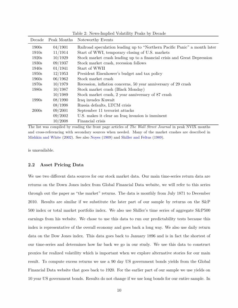
Table 2: News-Implied Volatility Peaks by DecadeDecade Peak Months Noteworthy Events

1900s 04/1901 Railroad speculation leading up to “Northern Pacific Panic” a month later1910s 11/1914 Start of WWI, temporary closing of U.S. markets1920s 10/1929 Stock market crash leading up to a financial crisis and Great Depression1930s 09/1937 Stock market crash, recession follows1940s 01/1941 Start of WWII1950s 12/1953 President Eisenhower’s budget and tax policy1960s 06/1962 Stock market crash1970s 10/1979 Recession, inflation concerns, 50 year anniversary of 29 crash1980s 10/1987 Stock market crash (Black Monday)

10/1989 Stock market crash, 2 year anniversary of 87 crash1990s 08/1990 Iraq invades Kuwait

08/1998 Russia defaults, LTCM crisis2000s 09/2001 September 11 terrorist attacks

09/2002 U.S. makes it clear an Iraq invasion is imminent10/2008 Financial crisis

The list was compiled by reading the front page articles of The Wall Street Journal in peak NVIX monthsand cross-referencing with secondary sources when needed. Many of the market crashes are described inMishkin and White (2002). See also Noyes (1909) and Shiller and Feltus (1989).

is unavailable.

2.2 Asset Pricing Data

We use two different data sources for our stock market data. Our main time-series return data are

returns on the Down Jones index from Global Financial Data website, we will refer to this series

through out the paper as “the market” returns. The data is monthly from July 1871 to December

2010. Results are similar if we substitute the later part of our sample by returns on the S&P

500 index or total market portfolio index. We also use Shiller’s time series of aggregate S&P500

earnings from his website. We chose to use this data to run our predictability tests because this

index is representative of the overall economy and goes back a long way. We also use daily return

data on the Dow Jones index. This data goes back to January 1896 and is in fact the shortest of

our time-series and determines how far back we go in our study. We use this data to construct

proxies for realized volatility which is important when we explore alternative stories for our main

result. To compute excess returns we use a 90 day US government bonds yields from the Global

Financial Data website that goes back to 1920. For the earlier part of our sample we use yields on

10 year US government bonds. Results do not change if we use long bonds for our entire sample. In

10

Table 3: Top Variance Driving n-gramsn-gram Variance Share, % Weight, % n-gram Variance Share, % Weight, %

stock 37.28 0.10 oil 1.39 -0.03market 6.74 0.06 banks 1.36 0.06stocks 6.53 0.08 financial 1.32 0.11war 6.16 0.04 _ u.s 0.88 0.05u.s 3.62 0.06 bonds 0.81 0.04tax 2.01 0.04 _ stock 0.80 0.03washington 1.78 0.02 house 0.77 0.05gold 1.46 -0.04 billion 0.67 0.06special 1.44 0.02 economic 0.64 0.05treasury 1.43 0.06 like 0.59 -0.05

We report the fraction of NVIX variance h (i) that each n-gram drives over the predict subsample as definedin (3), and the regression coefficient wi from (1), for the top 20 n-grams.

addition to this two time-series we also use the VXO and VIX indexes from the CBOE. They are

implied volatility indexes derived from a basket of option prices on the S&P500 (VIX) and S&P100

(VXO) indexes. The VIX time series starts in January 1990 and VXO starts in January 1986.

3 The Spirit of the Times

What drives investors’ concerns at different periods? Are these concerns reasonable? The NVIX

index we constructed relies on the relative frequency of words during each month in the sample. In

this section we investigate which words play an important role and try to describe the zeitgeist -

the spirit of the times.

We begin by calculating the fraction of NVIX variance that each word drives over the predict

subsample. Define vt (i) ≡ xt,iwi as the value of VIX predicted only by n-gram i ∈ {1..K}. We

construct

h (i) ≡ V ar (vt (i))∑j∈K V ar (vt (j)) (3)

as a measure of the n-gram specific variance of NVIX.7 Table 3 reports h (i) for the top variance

driving n-grams and the regression coefficient wi from the model (1) for the top variance n-grams.

Note that the magnitude of wi does not completely determine h (i) since the frequency of appear-

ances in the news interacts with w in (3).7Note that in general V ar (vt) 6=

∑j∈K V ar (vt (j)) due to covariance terms.

11

Table 4: Categories Total Variance ShareCategory Variance Share, % n-grams Top n-gram

Government 2.59 83 tax, money, ratesIntermediation 2.24 70 financial, business, bankNatural Disaster 0.01 63 fire, storm, aidsSecurities Markets 51.67 59 stock, market, stocksWar 6.22 46 war, military, actionUnclassified 37.30 373988 u.s, washington, gold

We report the percentage of NVIX variance (=∑i∈C h (i)) that each n-gram category C drives over the

predict subsample.

Clearly, when the stock market makes an unusually high fraction of front page news it is a

strong indication of high implied volatility. The word “stock” alone accounts for 37 percent of NVIX

variance. Examining the rest of the list, we find that stock market-related words are important as

well. This should not be surprising since when risk increases substantially, stock market prices tend

to fall and make headlines. War is the fourth most important word and accounts for 6 percent.

To study the principal word categories driving this variation, we classify n-grams into five

broad categories of words: Government, Intermediation, Natural Disasters, Securities Markets and

War. We rely on the widely used WordNet and WordNet::Similarity projects to classify words.8

WordNet is a large lexical database where nouns, verbs, adjectives and adverbs are grouped into

sets of cognitive synonyms (synsets), each expressing a distinct concept. We select a number of

root synsets for each of our categories, and then expand this set to a set of similar words which

have a path-based WordNet:Similarity of at least 0.5.

Table 4 reports the percentage of NVIX variance (=∑i∈C h (i)) that each n-gram category

drives over the predict subsample. Stock market related words explain over half the variation in

NVIX. War-related words explain 6 percent. Unclassified words explain 37 percent of the variation.

This large number speaks volumes about the limitations of manual word classification. Clearly

there are important features of the data, among the 374, 299 n-grams that the automated SVR

regression picks up. While these words are harder to interpret, they seem to be important in

explaining VIX behavior in-sample, and predicting it out-of-sample. In Section 4.6 we find that

this unclassified category is a significant predictor of future returns.8WordNet (Miller, 1995) is available at http://wordnet.princeton.edu. WordNet::Similarity (Pedersen, Patward-

han, and Michelizzi, 2004) is available at http://lincoln.d.umn.edu/WordNet-Pairs.

12

Table 5: News Implied Volatility Breakdown by CategoriesCategory (C) Mean Std Dev vt (C) = ρ0 + ρvt−1 (C) + εt

ρ SE(ρ) Half-life(ρ)

All (= NV IX) 4.06 4.65 0.82 0.02 3.53Government 0.86 0.39 0.68 0.02 1.78Intermediation 0.42 0.56 0.73 0.02 2.24Natural Disaster -0.01 0.03 0.18 0.03 0.40Securities Markets 3.15 2.45 0.89 0.01 6.00War 0.33 0.59 0.90 0.01 6.71Unclassified 8.63 3.19 0.77 0.02 2.61

We report the mean, standard deviation of monthly NVIX broken down by categories over the entire sample.For each n-gram category C, vt (C) ≡ xt ·w (C) is the value of demeaned VIX predicted only by n-gramsbelonging to C, where w (C) is w estimated from (1) with entries that are not part of category C zeroed-out.Also reported are estimates, standard errors, and implied half-lives (in months) from a AR(1) time-seriesmodels. Half-life is the number of months until the expected impact of a unit shock is one half, i.e.ρhalf−life = 1

2 .

3.1 NVIX is a Reasonable Proxy for Disaster Concerns

We use NVIX to proxy for the disaster probability in our investigation of return predictability

that follows in Section 4. Before doing so, we would like to gauge whether doing so is reasonable.

One way to answer this question is to ask what word categories drive NVIX variation in different

periods, and whether these words coincide with our sense of the events that defined each era.

To answer this question we construct separate NVIX time-series implied by each category. For

each n-gram category C, vt (C) ≡ xt ·w (C) is the value of VIX predicted only by n-grams belonging

to C. That is, w (C) is w estimated from (1) with entries that are not part of category C zeroed-

out. Table 5 reports means and standard deviations for NVIX and a breakdown by categories. We

find that Securities Markets are the most volatile component with a standard deviation of 2.96.

The unclassified category has about half the volatility of NVIX itself.

Figure 2 plots five year rolling variance estimates for each category, scaled by total NVIX

variance centered around each month. We exclude unclassified words because those would make

in-sample and out-of-sample comparisons less meaningful due to differences in estimation error.

We observe that Securities Markets related words drive the lion’s share of variance circa 1900

leading up to the panic of 1907. Stock market coverage drives a relatively high share of the variance

around the 1929, 1962, and 1987 market crashes. The high-tech boom and bust circa 2000 are clearly

13

Figure 2: News implied Volatility Variance Components

1900 1925 1950 1975 20000.0

0.2

0.4

0.6

0.8

1.0

Rel

ativ

eF

ract

ion

ofV

aria

nce

Securities Markets

War

Government

Intermediation

Natural Disaster

Stacked plot of five year rolling variance estimates for each category, scaled by total NVIX variance centeredaround each month excluding unclassified words.

visible.

Interestingly, variation in NVIX due to Government-related words really picks up in the later

days of the Great Depression when the U.S. government started playing a bigger role as New Deal

policies were implemented. WWII coverage sidelined this trend which continued once the war

stopped. Intermediation-related news dominates NVIX variance when expected, mostly during

financial crises. Apparent in the figure are the panic of 1907, the Great Depression of the 1930s,

the Savings & Loans crisis of the 1980s and the Great Recession of 2008.

War-related words drive a large share of variance around World War I and more than half of

the variance during World War II. Wars are clearly a plausible driver of disaster risk because they

can potentially destroy a large amount of both human and physical capital and redirect resources.

Figure 3 plots the NVIX War component over time. The index captures well the ascent into and

fall out of the front-page of the Journal of important conflicts which involved the U.S. to various

degrees. A common feature of both world wars is an initial spike in NVIX when war in Europe

14

Figure 3: News implied Volatility due to War-related Words

1900 1925 1950 1975 2000-1

0

1

2

3

4

5

NV

IX@W

arD

predict test train

Dots are monthly NVIX due only to War-related words vt (Wars) = xt ·w (Wars). Shaded regions are U.S.wars, specifically the American-Spanish, WWI, WWII, Korea, Vietnam, Gulf, Afghanistan, and Iraq wars.

starts, a decline, and finally a spike when the U.S. becomes involved.

The most striking pattern is the sharp spike in NVIX in the days leading up to U.S. involvement

in WWII. The newspaper was mostly covering the defensive buildup by the U.S. until the Japanese

Navy’s surprise attack at Pearl Harbor on December 1941. Following the attack, the U.S. actively

joined the ongoing War. NV IX[War] jumps from 0.87 in November to 2.86 in December and

mostly keeps rising. The highest point in the graph is the Normandy invasion on June 1944 with

the index reaching 4.45. The Journal writes on June 7, 1944, the day following the invasion:

“Invasion of the continent of Europe signals the beginning of the end of America’s wartime way of

economic life.” Clearly a time of elevated disaster concerns. Thus, NVIX captures well not only

whether the U.S. was engaged in war, but also the degree of concern about the future prevalent at

the time.

We find it quite plausible that changes in the disaster probability perceived by the average

investor would coincide with stock market crashes, world wars and financial crises. Since these are

15

exactly the times when NVIX varies due to each of these concerns, we find it is a plausible proxy

for disaster concerns.

3.2 Attention Persistence

How persistent is the attention given to each category over time? One might imagine that following

a stock market crash, the average investor, and the media who caters to him, pays closer attention

to the stock market. Malmendier and Nagel (2011) document that individuals who experience low

stock market returns are less willing to take financial risk, are less likely to participate in the stock

market, invest a lower fraction of their liquid assets in stocks, and are more pessimistic about future

stock returns. Thus such important events and the attention they draw can have long-lasting effects

on the average investor and the provision of capital in the economy. But how long exactly do these

effects last?

Table 5 reports persistence estimates for NVIX and a breakdown by categories. The composite

NVIX has a half-life of 3.53 months, but this is not the case for all word categories. Since the

standard errors imply a tight confidence interval around the autocorrelation ρ estimates, we can

statistically differentiate between them. Economic news is much more transitory compared to

Government coverage which remains front-page news that drives NVIX for extended periods of

time.

The most striking result in Table 5 is the large persistence in front-page attention given to

Securities Markets and War. A ρ of 0.89 implies that six months after an increase in NVIX

coinciding with securities market attention, half of the increase remains. Wars have statistically

the same high degree of persistence. Our estimates show that war attention builds up gradually

and keeps driving investors’ concerns long after the soldiers come home. Figure 3 makes this point

graphically. Though harder to visualize for recent conflicts, we can see quite clearly, that after all

four conflicts marked by shaded regions in the early part of the sample, war coverage declines only

gradually.

An important question is whether this persistence in peoples’ concerns is a reflection of the true

underlying disaster probability dynamics, or is a reflection of peoples’ past experiences shaping their

concerns and views about risk (Malmendier and Nagel, 2011). From an asset pricing perspective

it does not really matter if disaster concerns move because past experiences are salient to them or

16

because the true disaster probability is moving around. Prices reflect peoples shifting perception

of this risk. Table 5 shows that the attention paid to these disasters is variable and persistent, in

Section 4 we ask if these concerns are reflected in asset prices, and use the few disasters that we

have in sample to study if these concerns are rational or driven by salience of personal experiences

as in Malmendier and Nagel (2011).

4 Time-Varying Disaster Concerns

In this section we formally test the hypothesis that time-variation in disaster risk was an impor-

tant driver of variation in expected returns in this last century. We start with our main findings

and provide an intuitive interpretation of our empirical setting, followed by a rigorous theoretical

motivation for our regression specifications. We then discuss the identification of economic disas-

ters, explore and rule out alternative stories, and finally, examine the plausibility of the estimated

persistence and variation in disaster probability.

4.1 Main Results

The time-varying disaster risk explanation of asset pricing puzzles has two key empirical predictions

regarding asset prices: (i) periods of high rare disaster concerns are periods when put options on

the market portfolio prices are abnormally expensive, and (ii) these periods are followed either by

economic disasters or above average excess returns on the market portfolio. Since disaster concerns

are unobservable, we test these two predictions jointly. Specifically we test if periods of high option

prices are followed by disasters or periods of above average excess returns.

We formally motivate our empirical strategy in the next section, but it boils down to testing if

NVIX predicts future returns in paths without disasters, and if NVIX has information regarding

future disasters. To implement these two tests we first construct disaster dummies IDt→t+T which

turn on if there is a month classified as a disaster during the period t to t+ T , t not inclusive. We

then test if NV IX predicts future excess returns after we exclude disaster periods.

Table 6 shows that in the short-sample for which option prices are available the results are

weak. In the sample for which VIX is available, the implied volatility index predicts excess returns

in the one month to three months horizons. However, VIX was abnormally low just before the sole

17

Table 6: Return Predictability: Short Sample Testsret→t+T = β0 + β1X

2t + εt+T if IDt→t+T = 0

Independent Variable NVIX VXO VIX

Sample Period 1986-2009 1990-2009 1986-2009 1990-2009

Dependent Variable β1 R2 β1 R2 β1 R2 β1 R2

t(β1) Nt t(β1) Nt t(β1) Nt t(β1) Nt

ret→t+1 0.12 0.41 0.11 0.44 0.12 0.81 0.13 0.65[0.6] 284 [0.53] 236 [0.95] 285 [0.65] 237

ret→t+3 0.13 1.50 0.13 1.80 0.12* 2.36 0.16 3.29[1.21] 282 [1.14] 234 [1.75] 283 [1.59] 235

ret→t+6 0.12* 2.65 0.11 2.94 0.07 2.02 0.12* 4.14[1.72] 279 [1.59] 231 [1.56] 280 [1.92] 232

ret→t+12 0.07 1.84 0.08 2.84 0.05 1.71 0.08 2.94[1.07] 273 [1.3] 225 [1.09] 274 [1.32] 226

ret→t+24 0.04 0.95 0.03 0.77 0.02 0.41 0.02 0.30[0.64] 261 [0.56] 213 [0.39] 262 [0.29] 214

Reported are monthly return predictability regressions based on news implied volatility (NVIX), S&P 100options implied volatility (VXO), and S&P 500 options implied volatility (VIX). The sample excludes anyperiod with an economic disaster (ID

t→t+T = 1). Month t is classified as an economic disaster if the crash-index of month t is large than the crash index of 98.5% of the months in the period 1896− 2009. The crashindex is described in Section 4.2, and is the product of market return in the month t and economic growthin a six month window succeeding month t for months which the market return is negative. The dependentvariables are annualized log excess returns on the market index. The first and third columns report resultsfor the sample period for which VXO is available, while the second and fourth columns are for the sampleperiod for which VIX is available. t-statistics are Newey-West corrected with number of lags/leads equal tothe size of the return forecasting window.

economic disaster in 2008, what does not reject the time-varying disaster risk story but suggests

return predictability is the result of other economic forces. If we consider a slightly longer sample

for which the VXO implied volatility index on the S&P 100 is available, the evidence for return

predictability becomes somewhat weaker still.

This mixed evidence motivates our exercise. While we do not have new options data to bring

to bear, we use NVIX to extrapolate investors disasters concerns. Our test of the time-varying

disaster concern hypothesis is a joint test that NVIX measures investors disaster concerns and that

disaster concerns drive expected returns on our test asset, the S&P 500. Hence, a failure to reject

the null can either mean NVIX does not accurately measures disaster concerns or disaster concerns

do not drive expected returns. NVIX largely inherits the behavior of VIX and VXO in the sample

18

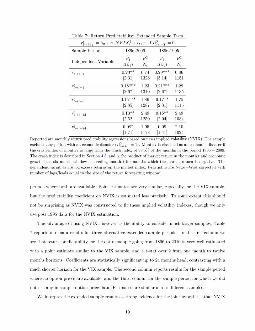
Table 7: Return Predictability: Extended Sample Testsret→t+T = β0 + β1NV IX

2t + εt+T if IDt→t+T = 0

Sample Period 1896-2009 1896-1995

Independent Variable β1 R2 β1 R2

t(β1) Nt t(β1) Nt

ret→t+1 0.23** 0.74 0.29*** 0.86[2.31] 1328 [3.14] 1151

ret→t+3 0.18*** 1.23 0.21*** 1.29[2.67] 1310 [2.67] 1135

ret→t+6 0.15*** 1.86 0.17** 1.75[2.85] 1287 [2.31] 1115

ret→t+12 0.13** 2.49 0.15** 2.49[2.52] 1250 [2.04] 1084

ret→t+24 0.08* 1.95 0.09 2.10[1.71] 1178 [1.41] 1024

Reported are monthly return predictability regressions based on news implied volatility (NVIX). The sampleexcludes any period with an economic disaster (ID

t→t+T = 1). Month t is classified as an economic disaster ifthe crash-index of month t is large than the crash index of 98.5% of the months in the period 1896− 2009.The crash index is described in Section 4.3, and is the product of market return in the month t and economicgrowth in a six month window succeeding month t for months which the market return is negative. Thedependent variables are log excess returns on the market index. t-statistics are Newey-West corrected withnumber of lags/leads equal to the size of the return forecasting window.

periods where both are available. Point estimates are very similar, especially for the VIX sample,

but the predictability coefficient on NVIX is estimated less precisely. To some extent this should

not be surprising as NVIX was constructed to fit these implied volatility indexes, though we only

use post 1995 data for the NVIX estimation.

The advantage of using NVIX, however, is the ability to consider much larger samples. Table

7 reports our main results for three alternative extended sample periods. In the first column we

see that return predictability for the entire sample going from 1896 to 2010 is very well estimated

with a point estimate similar to the VIX sample, and a t-stat over 2 from one month to twelve

months horizons. Coefficients are statistically significant up to 24 months head, contrasting with a

much shorter horizon for the VIX sample. The second column reports results for the sample period

where no option prices are available, and the third column for the sample period for which we did

not use any in sample option price data. Estimates are similar across different samples.

We interpret the extended sample results as strong evidence for the joint hypothesis that NVIX

19

Table 8: Disaster Predictability: Extended Sample TestsIDt→t+T = β0 + β1NV IX

2t−1 + εt

Sample Period 1896-2009 1896-1994 1938-2009

Quantities β1(×100) R2 β1(×100) R2 β1(×100) R2

t(β1) Nt t(β1) Nt t(β1) Nt

IDt→t+1 0.14*** 3.55 0.15*** 2.45 0.08 4.39[3.49] 1367 [3.28] 1187 [1.3] 863

IDt→t+3 0.19*** 4.02 0.20*** 3.32 0.09 2.81[3.52] 1367 [2.86] 1187 [1.26] 863

IDt→t+6 0.24*** 4.92 0.29*** 4.95 0.08 1.60[3.2] 1367 [2.58] 1187 [1.15] 863

IDt→t+12 0.28** 4.60 0.35** 5.23 0.07 0.63[2.49] 1367 [2.06] 1187 [0.8] 863

IDt→t+24 0.24 2.30 0.38 4.08 -0.04 0.14[1.5] 1367 [1.59] 1187 [0.34] 863

ND 13 12 2

Reported are monthly return predictability regressions based on news implied volatility (NVIX). The depen-dent variable is the dummy variable ID

t→t+T that turns if there was an economic disaster between months t(excluding) and t + T on sample excludes any period with an economic disaster (ID

t→t+T = 1). Month t isclassified as an economic disaster if the crash-index of month t is large than the crash index of 98.5% of themonths in the period 1896− 2009. The crash index is described in Section 4.3, and is the product of marketreturn in the month t and economic growth in a six month window succeeding month t for months whichthe market return is negative. t-statistics are Newey-West corrected with number of lags/leads equal to thesize of the disaster forecasting window.

measures disaster concerns and time-variation in disaster concerns drive expected returns. The

coefficient estimates imply substantial predictability with a one standard deviation increase in

NV IX2 leading to σNV IX2 × β1 = 21.66 × 0.23 = 5% higher annualized excess returns in the

following month. At the annual frequency excess returns are 2.80% higher. Unsurprisingly, R-

squares are small and attempts to exploit this relationship carry large risks even in samples without

economic disasters. Forecasting coefficients are monotonically decreasing in the forecasting horizon,

consistent with the fact that disaster concerns are persistent but substantially less persistent than

alternative return predictors such as dividend yields and equivalents. For disaster concerns have

a mean reversion coefficient of .79 at the monthly frequency compared to .98 for the the dividend

yield.

A second prediction of the time-varying disaster concerns hypothesis is that disaster concerns

20

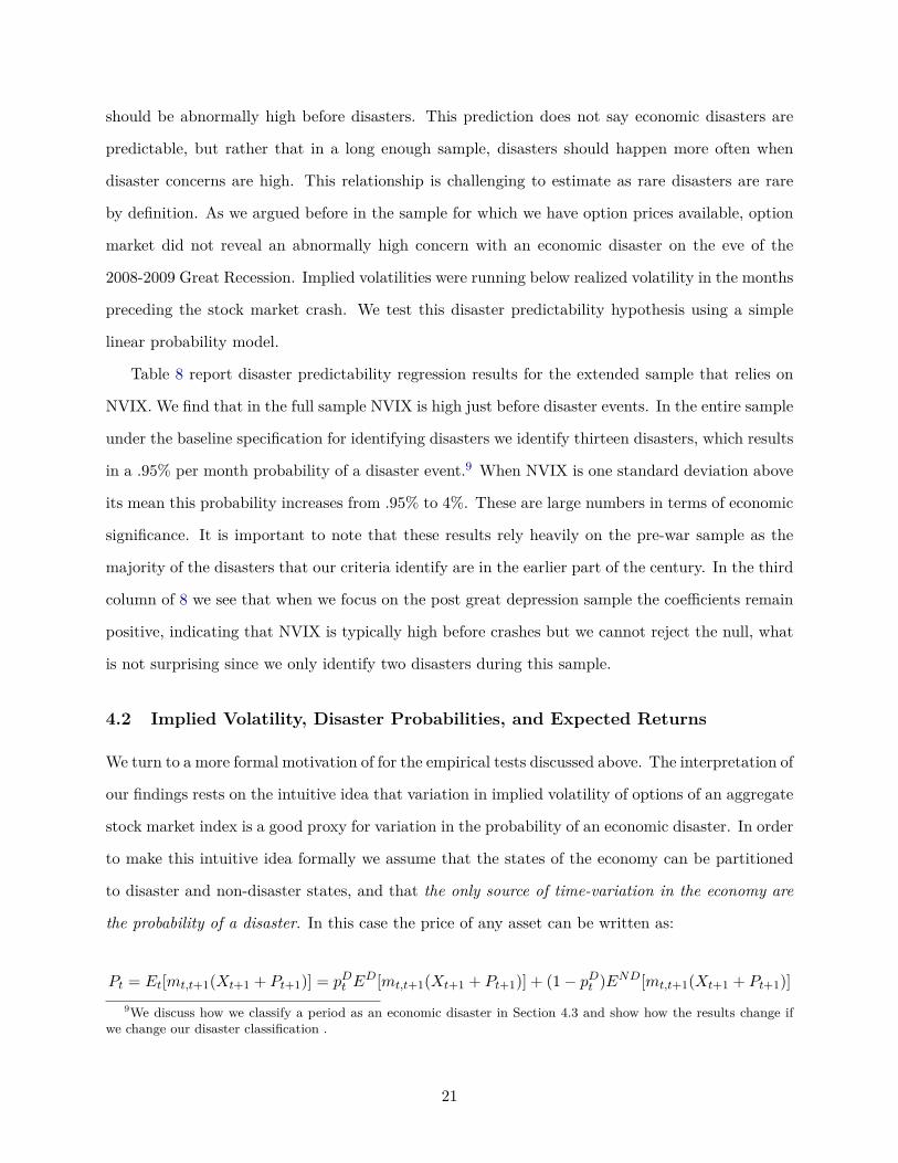
should be abnormally high before disasters. This prediction does not say economic disasters are

predictable, but rather that in a long enough sample, disasters should happen more often when

disaster concerns are high. This relationship is challenging to estimate as rare disasters are rare

by definition. As we argued before in the sample for which we have option prices available, option

market did not reveal an abnormally high concern with an economic disaster on the eve of the

2008-2009 Great Recession. Implied volatilities were running below realized volatility in the months

preceding the stock market crash. We test this disaster predictability hypothesis using a simple

linear probability model.

Table 8 report disaster predictability regression results for the extended sample that relies on

NVIX. We find that in the full sample NVIX is high just before disaster events. In the entire sample

under the baseline specification for identifying disasters we identify thirteen disasters, which results

in a .95% per month probability of a disaster event.9 When NVIX is one standard deviation above

its mean this probability increases from .95% to 4%. These are large numbers in terms of economic

significance. It is important to note that these results rely heavily on the pre-war sample as the

majority of the disasters that our criteria identify are in the earlier part of the century. In the third

column of 8 we see that when we focus on the post great depression sample the coefficients remain

positive, indicating that NVIX is typically high before crashes but we cannot reject the null, what

is not surprising since we only identify two disasters during this sample.

4.2 Implied Volatility, Disaster Probabilities, and Expected Returns

We turn to a more formal motivation of for the empirical tests discussed above. The interpretation of

our findings rests on the intuitive idea that variation in implied volatility of options of an aggregate

stock market index is a good proxy for variation in the probability of an economic disaster. In order

to make this intuitive idea formally we assume that the states of the economy can be partitioned

to disaster and non-disaster states, and that the only source of time-variation in the economy are

the probability of a disaster. In this case the price of any asset can be written as:

Pt = Et[mt,t+1(Xt+1 + Pt+1)] = pDt ED[mt,t+1(Xt+1 + Pt+1)] + (1− pDt )END[mt,t+1(Xt+1 + Pt+1)]

9We discuss how we classify a period as an economic disaster in Section 4.3 and show how the results change ifwe change our disaster classification .

21

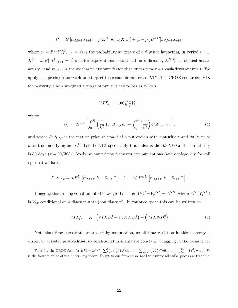
Pt = Et[mt,t+1Xt+1] = ptED[mt,t+1Xt+1] + (1− pt)END[mt,t+1Xt+1]

where pt = Prob(IDt→t+1 = 1) is the probability at time t of a disaster happening in period t + 1,

ED[·] ≡ E[·|IDt→t+1 = 1] denotes expectations conditional on a disaster, END[·] is defined analo-

gously , and mt,t+1 is the stochastic discount factor that prices time t+ 1 cash-flows at time t. We

apply this pricing framework to interpret the economic content of VIX. The CBOE constructs VIX

for maturity τ as a weighted average of put and call prices as follows:

V IXt,τ = 100√

1τVt,τ ,

where

Vt,τ = 2erf τ[∫ F0

0

( 1k2

)Putt,τ,kdk +

∫ ∞k0

( 1k2

)Callt,τ,kdk

], (4)

and where Putt,τ,k is the market price at time t of a put option with maturity τ and strike price

k on the underlying index.10 For the VIX specifically this index is the S&P500 and the maturity

is 30 days (τ = 30/365). Applying our pricing framework to put options (and analogously for call

options) we have,

Putt,τ,k = ptED[mt,t+τ [k − St+τ ]+

]+ (1− pt)END

[mt,t+τ [k − St+τ ]+

].

Plugging this pricing equation into (4) we get Vt,τ = pt,τ (V Dτ −V ND

τ )+V NDτ , where V D

τ (V NDτ )

is Vt,τ conditional on a disaster state (non disaster). In variance space this can be written as.

V IX2t,τ = pt,τ

(V IXD2

τ − V IXND2τ

)+(V IXND2

τ

)(5)

Note that time subscripts are absent by assumption, as all time variation in this economy is

driven by disaster probabilities, so conditional moments are constant. Plugging in the formula for

10Formally the CBOE formula is Vt = 2erf τ[∑k0

k=0

(∆kk2

)Putt,τ,k +

∑∞k=k0

(∆kk2

)Callt,τ,k

]−(F0k0− 1)2, where F0

is the forward value of the underlying index. To get to our formula we need to assume all strike prices are tradable.

22

VIX and rearranging we get a neat link between VIX and disaster probabilities:

pt,τ =V IX2

t,τ − V IXND2τ

V IXD2τ − V IXND2

τ

. (6)

This equation should be intuitive, V IXD2τ − V IXND2

τ measures the difference in risk-neutral

variance between disaster and non disaster states. If the gap between current VIX and normal

times VIX is large, it indicates the disaster probability is high. For example, in an economy where

return volatility is constant V IXND2τ is equal to return volatility. V IXD2

τ on the other hand is a

function of the risk-neutral disaster size, being larger if the expected disaster is large or if people

are more risk-averse with respect to disasters. Using this same pricing framework we show in the

Appendix that expected excess returns are approximately linear in disaster probabilities

Et[Ret+τ ] ≈ END[Ret+τ ]−(ED[mt,t+τR

et+τ ]

END[mt,t+τ ] − ED[Ret+τ ])pt,τ (7)

where the first term inside the brackets is the ex-ante pricing implications of economic disasters

and in the second term we have their ex-post cash-flow consequences. Note for example, in the

case of risk-neutrality both terms cancel out and there are no expected return consequences of

disaster probability variation. It is important to note these two effects work against each other,

with higher probabilities leading to higher expected returns, but also leading to higher expected

losses. Particularly challenging from an estimation stand point is the estimation of expected losses

that can only be estimated when a rare disaster actually happens. This means any attempt to

estimate relationship (7) directly will be highly sensitive to the realized disasters in the sample. A

more informative approach is to decompose the test of equation (7) in two, first we test if disaster

probabilities predict expected returns in paths without disasters, i.e.

ENDt [Ret+τ ] ≈ END[Ret+τ ]−(ED[mt,t+τR

et+τ ]

END[mt,t+τ ]

)pt,τ , (8)

which can be more reliably estimated because it only depends on the path of disaster concerns and

not actual disaster realizations. Second, we test the ex-post cash-flow effect by testing if disaster

probabilities actually predict disasters:

23

Et[IDt→t+τ ] = pt,τ . (9)

Equations (8) and (9) form the basis of our empirical analysis. It is important to emphasize

that the neat one-to-one link between disaster probabilities and VIX are a direct consequence of

the assumption that there are no other sources of time-variation in the economy, and in particular

that ENDt [mt,t+τ ] and EDt [mt,t+τ ] are constant, but not the same. A natural question is whether

our setup can distinguish between movements in the natural and risk-neutral probability of disas-

ters. While in this general case it is challenging to infer anything from the return predictability

regressions, the disaster predictability regressions do not depend on anything but variation in the

natural probability of a disaster, and allows us to distinguish between the two. We use this insight

in Section 4.7.

4.3 Economic Disasters

This more powerful approach requires us to take a stand on what a disaster is which requires the

econometrician’s judgment. The time-varying disaster risk hypothesis is really about macroeco-

nomic disasters, measured by sharp drops in consumption. The main challenge to use economic

activity data to test the time-varying disaster risk hypothesis is to get the timing of the disaster

arrival right. When exactly did investors become aware the Great Depression was happening? One

natural answer is “Black Monday”. But was the Great Depression really one terrible rare event

people learned about on October 29? or was it a sequence of three or four bad events? Information

embedded in market prices are a natural channel to detect the timing at which investors realized

what was happening, and the extent to which the future drop in economic activity was already

anticipated. The cost of focusing on the stock-market to identify disasters is that we distance

ourselves from the economic disasters that the disaster risk literature has in mind, and shift the

focus towards statistical measurement of jumps in asset prices.

Our approach to identify disasters use both pieces of information, requiring that big stock

market drops be followed by large drops in economic activity. This approach has the advantage of

keeping the focus on macro-economic disasters, while using stock markets to identify the timing of

economic disasters. We construct a “disaster-index” Zt = min{rmt , 0} ×∆yt−1,t+5 ,where rmt is the

24

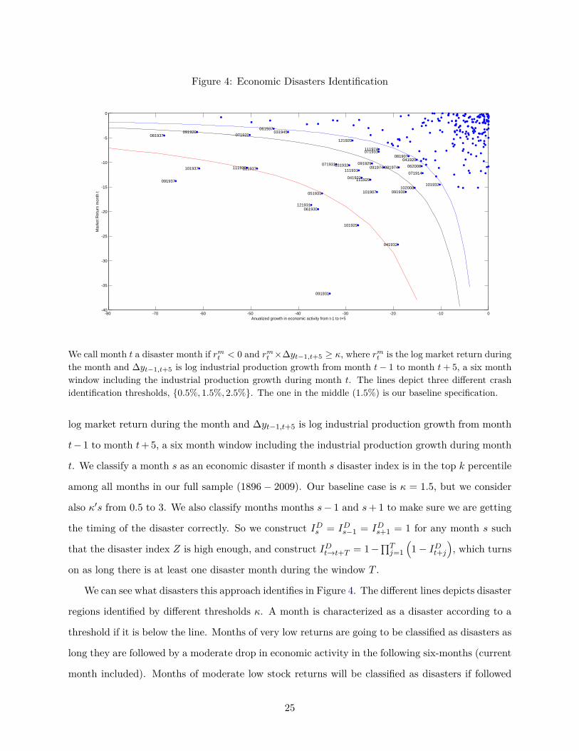
Figure 4: Economic Disasters Identification

-80 -70 -60 -50 -40 -30 -20 -10 0-40

-35

-30

-25

-20

-15

-10

-5

0

Anualized growth in economic activity from t-1 to t+5

Mar

ket R

etur

n m

onth

t

081907

101907

071914

041920

071920091920

111920

121920

091929

101929

111929

061930

091930

041931

051931

071931

091931

111931

121931

031932

041932

101932

071933

061937

081937

091937

101937 111937

031945

081974091974

111974

062008

102008

We call month t a disaster month if rmt < 0 and rm

t ×∆yt−1,t+5 ≥ κ, where rmt is the log market return during

the month and ∆yt−1,t+5 is log industrial production growth from month t− 1 to month t+ 5, a six monthwindow including the industrial production growth during month t. The lines depict three different crashidentification thresholds, {0.5%, 1.5%, 2.5%}. The one in the middle (1.5%) is our baseline specification.

log market return during the month and ∆yt−1,t+5 is log industrial production growth from month

t− 1 to month t+ 5, a six month window including the industrial production growth during month

t. We classify a month s as an economic disaster if month s disaster index is in the top k percentile

among all months in our full sample (1896 − 2009). Our baseline case is κ = 1.5, but we consider

also κ′s from 0.5 to 3. We also classify months months s− 1 and s+ 1 to make sure we are getting

the timing of the disaster correctly. So we construct IDs = IDs−1 = IDs+1 = 1 for any month s such

that the disaster index Z is high enough, and construct IDt→t+T = 1−∏Tj=1

(1− IDt+j

), which turns

on as long there is at least one disaster month during the window T .

We can see what disasters this approach identifies in Figure 4. The different lines depicts disaster

regions identified by different thresholds κ. A month is characterized as a disaster according to a

threshold if it is below the line. Months of very low returns are going to be classified as disasters as

long they are followed by a moderate drop in economic activity in the following six-months (current

month included). Months of moderate low stock returns will be classified as disasters if followed

25

by severe drops in economic activity in the six following months. This approach requires negative

signals from both economic activity and market returns to classify a month as disaster.

We use industrial production because it is the only measure of aggregate activity available

during our entire sample. It is available monthly since 1919 and annually since the beginning of the

sample. This leaves us with about 25 years (1896-1919) where we do not have a monthly measure

of economic activity. In this case we use gross domestic product which is measured quarterly

and interpolate linearly to obtain our measure of economic activity growth during the window of

interest11.

4.4 Robustness and Alternative Explanations

We next explore alternative explanations for our main results. One possibility is that NVIX is not

measuring variation in disaster concerns but rather current stock market volatility. According to

this story NVIX predicts returns because investors demand higher expected returns during more

volatile periods. We test this story by including stock market realized volatility as a control. The

results can be seen in Table 9. The coefficient on NVIX is slightly reduced and statistical significance

is also reduced, suggesting that at least a piece of the information embedded in NVIX is related to

current stock market volatility. However, the estimates show that NVIX has substantial additional

new information relative to current stock market volatility.

A second concern we have is that excluding disasters can mechanically generate predictability

in a world of time-varying volatility. The argument is as follows: suppose stock-market ex-ante

volatility is moving around in a predictable fashion. Our strategy to identify disasters is more

likely to identify disasters in periods of high ex-ante volatility. Suppose NVIX has information

about future volatility. Since disaster months are excluded from the regression, we are truncating

the left tail of the distribution exactly when volatility is higher. This mechanism would make our

proxy for volatility artificially predict returns. This story calls for a selection adjustment, which

we derive explicitly in Section A.2.

The intuition is analogous to studies where we only observe a selected sample. The standard

procedure is to control for this selection effect.12 In our exercise under the null we know the model11GDP data is from the NBER website.12For example, the Heckman selection model is a popular example of such selection corrections.

26

Table 9: Alternative Explanationsret→t+T = β0 + β1NV IX

2t + εt if IDt→t+T = 0

Volatility Truncation

Dependent Variable β1 R2 β1 − γ R2

t(β1) T t(β1 − γ) T

ret→t+1 0.17* 1.09 0.18* 0.74[1.67] 1328 [1.8] 1328

ret→t+3 0.12* 2.16 0.13** 1.23[1.67] 1310 [1.98] 1310

ret→t+6 0.13** 2.20 0.11** 1.86[2.28] 1287 [2.07] 1287

ret→t+12 0.10* 3.26 0.09* 2.49[1.9] 1250 [1.76] 1250

ret→t+24 0.07 2.19 0.04 1.95[1.44] 1178 [0.92] 1178

This table presents return predictability regressions based on our constructed NVIX series and stock marketvolatility. We measure stock market volatility σt using daily returns on the Dow Jones index within therelevant month. The sample excludes any period with an economic disaster. The dependent variable areannualized log excess returns. Each row and each column represents a different regression. In the row we havethe different forecasting horizons. In the first column we show the predictability coefficient of NVIX on futurereturns once we control for past realized volatility. In the second column we show the same predictabilitycoefficient after we subtract γ , the predictability coefficient implied by the time-varying truncation that ourprocedure of excluding disasters induces (for a full discussion see Section A.2) . t-statistics are Newey-Westcorrected with number of lags/leads equal to the size of the disaster forecasting window.

and the selection criteria. So there is no need for an instrument. In the first stage we estimate a

selection equation, where we estimate the ability of NVIX to predict the probability that a given

period is a disaster given the null where all that is happening is time-variation in volatility. This

specification gives a benchmark coefficient which is the coefficient that a regression from future

returns on NVIX should have if predictability was the result of this truncation story. In short,

instead of the null hypothesis being a zero coefficient, it is a new adjusted coefficient.

We develop this analysis in full in the appendix, but it is convenient to inspect an equation to

grasp the intuition of our test. We classify a month as a disaster if returns in the month are lower

than a threshold rt+1. Expected returns conditional on no disaster happening can be written as

E[rt+1|rt+1 ≥ rt+1] = µr + σt+1E[Wr,t+1|Wr,t+1 ≥rt+1 − E[rt+1]

σt+1] = µr + σt+1λ(rt+1),

27

Table 10: Post Depression Sample including Disastersret→t+T = β0 + β1NV IX

2t + εt

Sample Period 1896-2009 1938-2009

Excluding Disasters Including Disasters

Dependent Variable β1 R2 β1 R2

t(β1) T t(β1) T

ret→t+1 0.23** 0.74 0.12 0.21[2.31] 1328 [0.89] 863

ret→t+3 0.18*** 1.23 0.09 0.35[2.67] 1310 [0.69] 863

ret→t+6 0.15*** 1.86 0.14** 1.65[2.85] 1287 [2.2] 863

ret→t+12 0.13** 2.49 0.11** 2.03[2.52] 1250 [2.49] 863

ret→t+24 0.08* 1.95 0.10** 3.38[1.71] 1178 [2.49] 863

This table presents return predictability regressions based on our constructed NVIX series for two differentsubsamples. For the first columns we exclude any disaster from the sample, for the second column we do not.The dependent variable are annualized log excess returns on the market index. Each row and each columnrepresents a different regression. In the row we have the different forecasting horizons. In the first columnwe show the predictability coefficient of NVIX on future returns for the full sample excluding economicdisasters. In the second column we show the same coefficient without excluding disasters. t-statistics areNewey-West corrected with number of lags/leads equal to the size of the disaster forecasting window.

where λ(·) is commonly know as the mills ratio. According to the truncation rationale NVIX will

predict returns in paths without disasters to the extent it predicts σt+1λ(rt+1). Under the null we

have:

E[λ(rt)σt+1|NV IXt] = γ0 + γNV IXt (10)

So what this selection problem prescribes us to do is to run our main forecasting regression, and

test if β1 is different form γ, which is the coefficient of the regression of the truncated mean of the

return distribution on NVIX. If we could not reject equality of coefficients, than the time-varying

truncation hypothesis would be consistent with our results.

Results with the adjusted coefficients and t-stats are in Table 9. Both the statistical and eco-

nomic significance of the results stand once we adjust for this mechanical selection effect. Yet one

might still be concerned that the parametric structure that we impose on the return distribution

28

might not be doing a good job of capturing this truncation effect. One way to alleviate these con-

cerns is to focus on a sub-sample where there were fewer disasters but not exclude the disasters from

the sample. Since the majority of our disasters happen during the Great Depression, we focus on

a sub-sample starting in 1938, when the NBER officially declared the end of the Great Depression.

We run the return forecasting regression in the post depression sample without excluding disasters,

where only two economic disaster happened according to our baseline criteria. Since we are not

excluding disasters truncation concerns become mute.

The results in Table 10 show that the coefficients for horizons 6 to 24 months does not change

both in magnitude or in statistical significance. Coefficients for one and three months are slashed

by roughly half and lose their statistical significance. We will see in Table 11 that these short

horizons are also more sensitive to our criteria to identify economic disasters, but longer horizons

estimates remain significant.

Table 11 examines the sensitivity of our main return predictability results to different disaster

thresholds. Our baseline specification (κ = 1.5%) identifies thirteen disasters in our sample. The

more strict threshold identifies only six disasters. The results change somewhat depending on

the criteria used, with evidence for return predictability becoming weaker as we use a more strict

definitions of a disaster. This works exactly as expected as including disaster months in the return

predictability regression biases the coefficient downwards.

4.5 Time-Varying Expected Returns: are Rare Disasters the Whole Story?

Proponents of the rare disaster explanation suggest it can explain one of the key facts regarding

the time-series properties of stock-market returns, that the dividend yield on the market portfolio

predicts future returns far into the future. Our results suggest NVIX captures variation at different

frequencies than the dividend yield, but it seems only natural to horse-race them. If the concerns

encoded in NVIX are the same concerns reflected in dividend yields one of the variable should drive

the other out of the regression. We would expect that the variable measured with more more noise

to be driven out of the regression. And if not driven completely out we would expect the coefficient

magnitude to decrease.

Table 12 shows that if we focus on the whole sample this is approximately what happens,

with the coefficients on both NVIX and price to earnings ratios decreasing in the multivariate

29

Table11

:ReturnPr

edictability:

Disa

ster

Thresho

ldSe

nsitivity

re t→t+T

=β

0+β

1NVIX

2 t−1

+ε t

ifID t→t+T

=0

Disa

ster

threshold

κ=

0.5%

κ=

1%κ

=1.

5%κ

=2%

κ=

2.5%

κ=

3%

Dep

ende

ntVa

riable

β1

R2

β1

R2

β1

R2

β1

R2

β1

R2

β1

R2

t(β

1)T

t(β

1)T

t(β

1)T

t(β

1)T

t(β

1)T

t(β

1)T

re t→t+

10.13

0.24

0.16

*0.36

0.23

**0.74

0.24

**0.79

0.24

**0.80

0.32

***

1.32

[1.4]

1349

[1.66]

1340

[2.31]

1328

[2.37]

1316

[2.36]

1304

[4.28]

1289

re t→t+

30.09

0.28

0.10

0.38

0.18

***

1.23

0.18

***

1.26

0.18

***

1.35

0.22

***

1.75

[1.01]

1340

[1.1]

1325

[2.67]

1310

[2.68]

1293

[2.74]

1276

[3.36]

1251

re t→t+

60.13

**1.23

0.12

**1.23

0.15

***

1.86

0.14

***

1.72

0.14

***

1.81

0.16

***

2.04

[2.39]

1328

[2.34]

1307

[2.85]

1287

[2.76]

1264

[2.71]

1242

[2.69]

1205

re t→t+

120.12

***

2.23

0.13

***

2.47

0.13

**2.49

0.12

**2.28

0.11

**2.15

0.12

**2.11

[2.72]

1313

[2.74]

1281

[2.52]

1250

[2.44]

1215

[2.28]

1192

[2.04]

1135

re t→t+

240.10

**3.32

0.10

**3.46

0.08

*1.95

0.07

*1.99

0.07

1.83

0.06

1.08

[2.4]

1289

[2.34]

1233

[1.71]

1178

[1.65]

1129

[1.58]

1096

[1.14]

1003

ND

69

1317

2126

Thistablepresents

return

predictabilityregressio

nsba

sedon

ourconstruc

tedNVIX

serie

sfordiffe

rent

disaster

thresholds.The

sampleexclud

esan

ype

riodwith

anecon

omic

disaster.The

depe

ndentvaria

blearean

nualized

logexcess

returns,

whe

retheris

kfree

rate

andthereturn

serie

sare

from

Shiller.The

riskfree

rate

istheyieldon

tenyear

governmentbo

ndan

dthereturn

serie

sarereturnson

theS&

P500index.

t-statist

icsare

New

ey-W

estcorrected.

The

samplepe

riodis

1896

to2010.

30

Table 12: Price-to-Earnings Ratio Predictabilityret→t+T = β0 + β1NV IX

2t−1 + β2(PE )t−1 + εt if IDt→t+T = 0

Sample Period 1896-2010 1896-1994

Dependent β1 β2 R2 β1 β2 R2

Variable t(β1) t(β2) T t(β1) t(β2) T

ret→t+1 0.23** 0.74 0.29*** 0.86[2.31] 1328 [3.14] 1151

-0.50* 0.30 -0.68 0.29[1.79] 1328 [1.54] 1151

0.23** -0.47* 1 0.32*** -0.89* 1.34[2.25] [1.71] 1328 [3.24] [1.91] 1151

ret→t+3 0.18*** 1.23 0.21*** 1.29[2.67] 1310 [2.67] 1135

-0.50** 0.84 -0.67* 0.78[2.14] 1310 [1.81] 1135

0.17** -0.47** 1.98 0.24*** -0.81** 2.41[2.56] [2.04] 1310 [2.93] [2.17] 1135

ret→t+6 0.15*** 1.86 0.17** 1.75[2.85] 1287 [2.31] 1115

-0.48** 1.63 -0.64** 1.47[2.24] 1287 [1.98] 1115

0.15*** -0.45** 3.30 0.20*** -0.74** 3.68[2.68] [2.11] 1287 [2.63] [2.34] 1115

ret→t+12 0.13** 2.49 0.15** 2.49[2.52] 1250 [2.04] 1084

-0.56** 4.26 -0.79*** 4.24[2.5] 1250 [2.59] 1084

0.12** -0.53** 6.27 0.17** -0.86*** 7.40[2.23] [2.36] 1250 [2.33] [2.93] 1084

ret→t+24 0.08* 1.95 0.09 2.10[1.71] 1178 [1.41] 1024

-0.50** 7.70 -0.63** 6.10[2.22] 1178 [2.54] 1024

0.07 -0.49** 9.14 0.10* -0.66*** 8.77[1.48] [2.12] 1178 [1.67] [2.71] 1024

This table presents return predictability regressions based on our constructed NVIX series and price-to-earning ratios. The sample excludes any period with an economic disaster. The dependent variable areannualized log excess returns on the market index. Price-to-earnings ratios are from Shiller, where earningsare 10 years averages of S&P500 earnings.t-statistics are Newey-West corrected with number of lags/leadsequal to the size of the disaster forecasting window. The first column reports the results for our entire sampleperiod, and the second column for the sample period for which we did not use any in sample option pricedata.

31

specification. It is reassuring that the NVIX coefficient is always estimated more reliably than

the price to earnings ratio coefficient. With the difference being specially meaningful for shorter

horizons. However, comparing R2 across horizons we see that the predictive power of the two

different variables roughly adds up. This pattern is replicated across alternative sample periods,

and strongly suggests that these variables are measuring different things.

We interpret these results as saying disaster concerns, at least the ones we can measure though

NVIX, are not likely to be the whole explanation behind time-variation in expected returns. A

possibility put forth by Wachter (forthcoming) is that different disaster concerns might move at

different frequencies, generating return predictability at different frequencies. Under this story

VIX and price to earnings ratio would put different weights in these different concerns. We next

decompose NVIX by different types of disaster concerns and explore this possibility.

4.6 Which Concerns?

A question that our NVIX measure allows us to ask is exactly which concerns drive expected

returns. As discussed in Section 3, this requires some judgment in word classification, but has the

advantage of providing deeper insight into what drives asset prices. We use the word classification

and reproduce the analysis in Table 7 for each of the word categories.

In Table 13 the War, Government and Unclassified categories stand out. All three predict

returns in paths without disasters. Although the components have different coefficients, all have

similar economic significance with periods where NVIX due to wars is one standard deviation

above average being followed by 260 bps higher annual returns over the next three months. For

the Unclassified and Government categories this quantity is 300 and 254 bps respectively.

Table 13 means that months in which investors were paying abnormal attention to war or

government related topics they also demanded higher expected returns. In the case of attention to

Government there are two plausible interpretations of this relation: (i) investors might be paying

attention to the government because the government is responding to a shock, for example, the

spur of government activity that that happened after the bankruptcy of Lehman Brothers, (ii) or

because the government itself is generating the shock through mismanagement of policy. We cannot

distinguish these two stories, but we can say that in the past century periods where governments

were the focus of a lot of investor attention were periods of abnormally high expected returns.

32

Table13

:ReturnPr

edictability:

Which

Con

cerns?

re t→t+T

=β

0+β

1NVIX

2 [Category] t

+β

2σt+ε t

ifID t→t+T

=0

Category:

Nvix

War

Governm

ent

Interm

ediation

Natural

Disaster

Secu

rities

Markets

Unc

lassified

Dep

ende

ntβ

1R

2β

1R

2β

1R

2β

1R

2β

1R

2β

1R

2β

1R

2

Varia

ble

t(β

1)t(β

1)t(β

1)t(β

1)t(β

1)t(β

1)t(β

1)re t→t+

10.17

*1.09

1.25

**1.04

1.80

**0.99

-0.66

0.82

7.97

0.79

0.18

0.88

0.15

0.95

[1.67]

[2.52]

[2.02]

[0.75]

[0.57]

[1.39]

[1.07]

re t→t+

30.12

*2.16

1.36

***

2.64

1.82

**2.37

-0.03

1.72

4.44

1.73

0.05

1.74

0.12

2.03

[1.67]

[3.23]

[2.47]

[0.04]

[0.46]

[0.44]

[1.33]

re t→t+

60.13

**2.20

1.37

***

3.07

1.21

*1.68

-0.12

1.08

9.54

1.23

0.02

1.08

0.16

***

2.31

[2.28]

[3.41]

[1.72]

[0.18]

[1.11]

[0.13]

[2.62]

re t→t+

120.10

*3.26

1.21

***

4.99

1.07

2.81

0.15

1.91

7.64

2.08

0.02

1.89

0.11

**3.11

[1.9]

[3.78]

[1.46]

[0.31]

[1.07]

[0.13]

[2.01]

re t→t+

240.07

2.19

0.68

**3.20

1.22

*3.64

0.13

0.94

-0.39

0.90

0.02

0.93

0.06

1.74

[1.44]

[2.18]

[1.79]

[0.33]

[0.08]

[0.2]

[1.37]

Thistablepresents

return

pred

ictabilityregressio

nsba

sedon

NVIX

impliedby

divide

din

diffe

rent

n-gram

categorie

san

dpa

strealized

volatility

.The

sampleexclud

esan

ype

riodwith

anecon

omic

disaster.The

depe

ndentvaria

bles

arean

nualized

logexcess

returnson

themarketinde

x.Ea

chrow

andeach

columnrepresents

theresults

ofadiffe

rent

regressio

nwhe

reweon

lyrepo

rtthereturn

forecastingcoeffi

cientβ

1.t-statist

icsareNew

ey-W

est

correctedwith

lead

s/lags

equa

ltothesiz

eof

thedisaster

forecastingwindo

w..The

samplepe

riodis

1896

to2009.

33

However, in the case of War it is plausible to give a more forceful interpretation that investors

concerns about wars caused the higher expected returns. The reverse causality story here is un-

plausible. The time series pattern of War concerns appearing in Figure 3 is compelling and clearly

related to the timing of major armed U.S. conflicts.

The pattern that emerges from Table 13 suggests that concerns regarding the government

have a relatively short-lived impact on expected returns with a one standard deviation increase

in government leading to 250 bps over the following month, but only a 150 bps increase over the

following year (both quantities are annualized). War concerns, by contrast, barely decay going

from 290 bps (next month) to 280 bps (next year). This large heterogeneity in the horizon at which

these concerns matter lends some support to Wachter’s conjecture that different disaster concerns

operate at different frequencies. We find that War-related concern have a long-lasting impact on

expected returns, while Government-related concerns are focused mostly in shorter horizons.

4.7 Volatility, Persistence and Size of Disaster Concerns

In this section we connect the coefficient estimates from our two predictability specifications to

structural parameters of interest in the macro-finance literature. In particular our regressions

can recover the volatility and persistence of the disaster probability process, and the risk neutral

disaster size. We report our estimates for these quantities in Table 14. We explain formally where

our estimates come from and provide an economic interpretation.

Let us start with a small disaster probability linear approximation to equation (5)

V IX2t,τ ≈ V IXND2

t,τ + φpt,τ ,

where x denotes deviations from the unconditional mean and φ is an approximating constant

related to the unconditional difference in VIX in disaster versus normal times. If the disaster

probability process follows an AR(1) process with persistence parameter ρp, an OLS regression of

disaster dummies IDt→t+m on V IX2t,τ recovers plim(βDm) =

φV AR(pt,τ )∑m

j=1 ρjp

V ar( V IX2t,τ )

, which implies that

the ratio between coefficients of two different horizons mL and mS recovers the disaster probability

persistence ρp:

plim

(βDmLβDms

)=

1− ρmLp1− ρmSp

. (11)

34

Table 14: Disaster Risk: Persistence, Volatility and Size(a) Disaster Probability Persistence (b) Disaster Probability Persistence

Implied by Return Predictability Regressions Implied by Disaster Predictability Regressions

ρR ={x

∣∣∣∣∣mLβRmLmsβRms= 1−xmL

1−xmS

}mL = 3 mL = 6 mL = 12

ms = 1 0.90 0.89 0.90ms = 3 - 0.88 0.91ms = 6 - - 0.92

ρp ={x

∣∣∣∣∣βDmLβDms= 1−xmL

1−xmS

}mL = 3 mL = 6 mL = 12

ms = 1 >1 >1 >1ms = 3 - 0.89 0.92ms = 6 - - 0.94

(c) Disaster Probability and Expected Return Volatility (d) Risk Neutral Disaster Size12mσ(E[pt,m| NV IX2

t,τ ]) σ(END[ret+m|NV IX2

t,τ ])m = 1 4.2% 4.8%m = 3 6.2% 4.3%m = 6 5.7% 3.5%m = 12 4.3% 2.8%

∣∣∣∣ED[mt,t+1Ret+1]END[mt,t+1]

∣∣∣∣ =m12β

Rm

βDm

m = 1 132%m = 3 65%m = 6 64%m = 12 62%

We follow a similar strategy with the return predictability specification, but in this case a similar

computation only recovers the overall persistence of expected returns ρR:

plim

(mLβ

RmL

msβRms

)= 1− ρmLR

1− ρmSR. (12)

If disaster probability variation is the only driver of expected returns, this persistence should match

the one we recover from the disaster predictability specification (ρp = ρR). In general, however,

expected returns are also driven by time-variation is other sources of uncertainty ( V IXND2t,τ for

example captures movements in normal times risk-neutral volatility).

Table 14 panel (a) and (b) reports ρp estimates. First, we find a tight range of persistence

estimates implied by the return predictability specifications, ranging from 0.88 to 0.92. If we

exclude the results of the one-month specifications, the disaster probability specification suggests

very similar magnitudes with the point estimates ranging between 0.89 and 0.94. The estimates

that use the one-month regression coefficient imply explosive dynamics, which is a consequence of

the one-month regression estimate being substantially lower than estimates from longer horizons.

While the estimates strongly suggest disaster concerns are persistent, they are considerably smaller

than the numbers considered in the literature. For example, Gourio (2012) uses approximately

ρp = 0.96 at the monthly frequency, and Wachter (forthcoming) chooses ρp = 0.99 to match the

persistence of valuation ratios.

35

Let us now turn to the volatility of the disaster probability process. To estimate this volatil-

ity we follow a similar approach and identify variation in disaster probabilities from the disaster

predictability specification:

σ2p = V ar(E[pt,m|V IX2

t,τ ]) = (βDm)2V ar(V IX2t,τ ).

We can repeat a similar computation to back out the amount of expected return variation

detected by our measure. In panel (c) we report our estimates for the (annualized) volatility of

disaster probability shocks and expected returns shocks detected by NVIX. Point estimates range

from 4.2% to 6.2% for the volatility of disaster probability shocks, and from 2.8% to 4.8% for

expected return shocks. It is again useful to contrast these quantities with the parameter choice

currently used in the literature. Wachter (forthcoming) calibrates a continuous time model to

produce an unconditional standard deviation of σp ≈ 2.9% per year in disaster probability. Gourio

(2012) calibrates a discrete time model with an unconditional annual volatility of σp ≈ 2.3%.

Relative to the calibrations in the literature we find disaster concerns to be more volatile and less

persistent.

Both Wachter (forthcoming) and Gourio (2012) calibrations of σp were chosen to match the

volatility of realized returns given the rest of their parameter choices. In our empirical exercise we

explore this cross equation restriction between the return predictability and the disaster predictabil-

ity regressions imposed by the rare disaster risk model. This cross-equation restriction yields an

additional test of the time-varying disaster risk hypothesis. Under the hypothesis that all time-

variation in expected returns detected by VIX is driven by variation in the disaster probability, the

ratio between return and disaster predictability regression coefficients recovers the risk-adjusted

disaster size:

plim

(m12Eβ

Rm

βDm

)= −

ED[mt,t+1Ret+1]

END[mt,t+1] . (13)

Our point estimates for this quantity range from 62% to 132%, with an average point estimate

of 78%. The fact that we detect a much larger disaster size form the one-month horizon is yet

another reflection of the one-month disaster predictability regression detecting substantially lower

predictability than longer horizons.

36

Are these disaster sizes reasonable? We can compare these estimates with the Barro and

Ursua (2008) calibration based on a large sample of countries some of which experienced economic

disasters. In their calibration the average rare disasters have an average consumption drop of 22%,

agents have coefficient of relative risk aversion of 3.5, and average stock market drop of 32%. In

this case we have∣∣∣∣ED[mt,t+1Ret+1]END[mt,t+1]

∣∣∣∣ =∣∣∣∣ED[β( ct+1

ct)−γRet+1]

END[β( ct+1ct

)−γ ]

∣∣∣∣ ≈ ∣∣∣ (0.78)−3.5(−32%)0.94

∣∣∣ = 81%. This number is

in the same ballpark as our estimates. This indicates that the amount of predictability we detect

in expected returns is consistent with the amount of predictability given a reasonable calibration

of rare disasters.

5 Conclusion

This paper uses a text-based method to extend options-implied measures of disaster concerns back

to the end of the 19th century, bringing new data to bear on the time-varying rare disaster asset

pricing model. We show that news implied volatility is plausibly related with peoples concerns

about rare disasters. Using our proposed measure of disaster concerns we find that it predicts

expected returns and large economic disasters, consistent with a time-varying rare disaster risk

model. We find that shocks to disaster probabilities have a persistence of 0.9 at the monthly

frequency, consistent with half-life of five-months. These shocks are sizable with a one standard

deviation shock to the disaster probability (4%) being of the same magnitude as it’s unconditional

value (3%) at the quarterly frequency. Furthermore, we show that the amounts of predictability

we detect in future returns and future disasters are quantitatively consistent with each other.

Our NVIX index can be used in other studies where the short VIX sample limits the inferences

that can be drawn. The approach we take, of extending via text regression an economically desirable

variable, to periods or settings where it did not exist, can potentially be applied to other settings.

ReferencesAntweiler, Werner, and Murray Z. Frank, 2004, Is all that talk just noise? the information contentof internet stock message boards, Journal of Finance 59, 1259–1293.

Backus, D., M. Chernov, and I. Martin, 2011, Disasters implied by equity index options, Thejournal of finance 66, 1969–2012.

37

Baker, S.R., N. Bloom, and S.J. Davis, 2012, Measuring economic policy uncertainty, Workingpaper.

Barro, R.J., 2006, Rare disasters and asset markets in the twentieth century, The Quarterly Journalof Economics 121, 823–866.

, 2009, Rare disasters, asset prices, and welfare costs, The American Economic Review pp.243–264.

, E. Nakamura, J. Steinsson, and J.F. Ursua, 2009, Crises and recoveries in an empiricalmodel of consumption disasters, manuscript, June.

Barro, R.J., and J.F. Ursua, 2008, Consumption disasters in the twentieth century, The AmericanEconomic Review 98, 58–63.

Bollerslev, T., and V. Todorov, 2011, Tails, fears, and risk premia, The Journal of Finance 66,2165–2211.

Brown, Stephen J., William N. Goetzmann, and Stephen A. Ross, 1995, Survival, The Journal ofFinance 50, pp. 853–873.

Cherkassky, V., and Y. Ma, 2004, Practical selection of svm parameters and noise estimation forsvm regression, Neural networks 17, 113–126.

Drechsler, I., 2008, Uncertainty, time-varying fear, and asset prices, in AFA 2010 Atlanta MeetingsPaper.

, and A. Yaron, 2011, What’s vol got to do with it, Review of Financial Studies 24, 1–45.

Engelberg, Joseph, 2008, Costly information processing: Evidence from earnings announcements,Working paper.

Gabaix, X., 2012, Variable rare disasters: An exactly solved framework for ten puzzles in macro-finance, The Quarterly Journal of Economics 127, 645–700.

García, Diego, forthcoming, Sentiment during recessions, Journal of Finance.

Gourio, Francois, 2008, Time-series predictability in the disaster model, Finance Research Letters5, 191–203.

, 2012, Disaster risk and business cycles, American Economic Review 102, 2734–2766.

Hastie, Trevor, Robert Tibshirani, and Jerome Friedman, 2009, The elements of statistical learning(Springer) second edition edn.

Hoberg, Gerard, and Gordon Phillips, 2010, Product market synergies and competition in mergersand acquisitions: A text-based analysis, Review of Financial Studies 23, 3773–3811.

, 2011, Text-based network industries and endogenous product differentiation, Workingpaper.

Kelly, Bryan T., 2012, Tail risk and asset prices, Working Paper.

38

Kogan, S., D. Levin, B.R. Routledge, J.S. Sagi, and N.A. Smith, 2009, Predicting risk from financialreports with regression, in Proceedings of Human Language Technologies: The 2009 AnnualConference of the North American Chapter of the Association for Computational Linguistics pp.272–280. Association for Computational Linguistics.

Kogan, S., B. Routledge, J. Sagi, and N. Smith, 2010, Information content of public firm disclosuresand the sarbanes-oxley act, Working paper.

Loughran, T., and B. McDonald, 2011, When is a liability not a liability? textual analysis, dictio-naries, and 10-ks, The Journal of Finance 66, 35–65.

Malmendier, Ulrike, and Stefan Nagel, 2011, Depression babies: Do macroeconomic experiencesaffect risk taking?, The Quarterly Journal of Economics 126, 373–416.

Miller, G.A., 1995, Wordnet: a lexical database for english, Communications of the ACM 38, 39–41.

Mishkin, F.S., and E.N. White, 2002, Us stock market crashes and their aftermath: implicationsfor monetary policy, NBER Working paper.

Noyes, A.D., 1909, A year after the panic of 1907, The Quarterly Journal of Economics 23, 185–212.

Pedersen, Ted, Siddharth Patwardhan, and Jason Michelizzi, 2004, Wordnet::similarity - measuringthe relatedness of concepts, in Daniel Marcu Susan Dumais, and Salim Roukos, ed.: HLT-NAACL 2004: Demonstration Papers pp. 38–41 Boston, Massachusetts, USA. Association forComputational Linguistics.

Rietz, T.A., 1988, The equity risk premium a solution, Journal of monetary Economics 22, 117–131.

Shiller, R., and W. Feltus, 1989, Fear of a crash caused the crash, The New YorkTimes p. F3.

Tetlock, Paul, Maytal Saar-Tsechansky, and Sofus Macskassy, 2008, More than words: Quantifyinglanguage to measure firms’ fundamentals, Journal of Finance 63, 1437–1467.

Tetlock, Paul C., 2007, Giving content to investor sentiment: The role of media in the stock market,The Journal of Finance 62, 1139–1168.

Vapnik, N. Vladimir, 2000, The Nature of Statistical Learning Theory (Springer-Verlag, New York.).

Wachter, Jessica A., forthcoming, Can time-varying risk of rare disasters explain aggregate stockmarket volatility?, Journal of Finance.

A Appendix

A.1 Disaster Probability and Return Predictability

Following the framework we used to analyze the link between VIX and disaster probability, we split

states between disaster states and non disaster states. And consider the pricing of excess returns

39

between t and t+ τ , we have

0 = Et[mt,t+τR

et+τ]

0 = ptEDt [mt,t+τR

et+τ ] + (1− pt)ENDt [mt,t+τR

et+1]

Rearranging, we get

ENDt [Ret+τ ] = − 1ENDt [mt,t+τ ]

covNDt (mt,t+τ , Ret+τ )− pt+τ

(1− pt+τ )EDt [mt,t+τR

et+τ ]

ENDt [mt,t+τ ]

The first term is the standard risk adjustment, where assets that are negatively related to

the stochastic discount factor have higher equilibrium expected excess returns. The second term

captures the risk-adjustment and cash-flow effects of the possibility of a rare disaster. This asset

pricing restriction predicts that as long EDt [mt,t+τRet+τ ] < 0, periods of high disaster probabilities

will be be periods of high expected returns in the histories without disasters. If as in last section

we assume that the only source of variation are the disaster probabilities then,

ENDt [Ret+τ ] = − 1END[mt,t+τ ]cov

ND(mt,t+τ , Ret+τ )− pt

(1− pt)ED[mt,t+τR

et+τ ]

END[mt,t+τ ]

Given that rare disasters are rare, we can approximate this relationship around p ≈ 0,

ENDt [Ret+τ ] ≈ END[Ret+τ ]−ED[mt,t+τR

et+τ ]

END[mt,t+τ ] pt

Putting together the fact that expected returns are approximately linear in disaster probabilities

and from last section that disaster probabilities are proportion to the VIX squared, we have that

expected returns should be proportional to VIX squared. In fact plugging equation we get pt,τ =V IX2

t,τ−V IXND2τ

V IXD2τ−V IXND2

τ, and therefore

ENDt [Ret+1] ≈ END[Ret+1]−ED[mt+1R

et+1]

END[mt+1]

(V IX2

t,τ − V IXND2τ

V IXD2τ − V IXND2

τ

)= β0 + β1

(V IXt

100

)2τ

40

A.2 Truncation

A concern that we have regarding our approach to identify disasters is that the predictability results

in non-crash periods might be a mechanical artifact of truncating the left tail of the distribution

during periods of higher volatility. If NVIX is a proxy for future stock-market volatility periods of

higher volatility where no disaster was observed will be period of artificially higher returns. This

will me a mechanical of artifact of the truncation. Testing this hypothesis is fairly straightforward.

Consider the following model featuring time-varying volatility but constant expected returns:

σ2t+1 = µσ + ρσ2

t + ω√σ2tWσ,t+1

rt+1 = µr + σt+1Wr,t+1

So in this counter-factual economy there is no real predictability and there is no sense that very

low returns are special. But suppose in this environment we use threshold r to split the sample in

disaster periods and normal times. In this case we would have average returns in non-crash periods

given by:

E[rt+1|rt+1 ≥ r, σt+1] = µr + σt+1E[Wr,t+1|Wr,t+1 ≥r − µrσt+1

] = µt + σt+1λ(r)

λ(r) is the well known Mills ratio, which is basically the mean of a truncated variable. In the context

of our example we know exactly how months were selected as disasters, so we know the threshold

r. If NV IXt is correlated with future volatility the truncation will lead us to find predictability

when in fact there is none. In this case conditional expectations are given by:

E[rt+1|rt+1 ≥ r,NV IXt] = µr + E[σt+1λ(r)|NV IXt]

Focusing on linear expectations we can write this as:

E[λ(r)σt+1|NV IXt] = γ0 + γ1NV IXt

E[rt+1|rt+1 ≥ r,NV IXt] = µr + γ0 + γ1NV IXt

41

The above expression tell us that in order to test the time-varying rare disaster story against the

truncation story is enough to test the NVIX coefficient against γ1 instead of zero. If the estimated

coefficient is larger than γ1λ(r) we can reject the null that the predictability during periods without

disasters is induced by this truncation effect. In our procedure to identify disasters we use a joint

criteria of future economic activity and market returns so this procedure is not readily applicable.

The more general procedure has similar intuition. Instead of fixed, the disaster threshold is higher

when economic conditions are particularly bad:

E[rt+1|rt+1 ≥ r(Yt+1), Yt+1] = µr + σt+1E[Wr,t+1|Wr,t+1 ≥r(Yt+1)− µr

σt+1] = µt + σt+1λ(r(Yt+1))

It then follows E[E[rt+1|rt+1 ≥ r(Yt+1), Yt+1]|NV IXt] = µr + γ0 + γ1NV IXt, where γ1 is the

coefficient of an OLS regression of σt+1λ(r(Yt+1)) on NV IXt. In the general case rejecting the

non-predictability null amounts to rejecting γ1 instead of zero.

A.3 Alternative Text-based Analysis Approaches

We estimate the relationship between news and volatility, disaster concerns and returns in our

dataset using support vector regression (1). SVR overcomes the main challenge, which is the large

dimensionality of the feature space (number of unique n-grams). Our approach lets the data speak

without much human interaction. Two alternative approaches have been suggested by previous

literature.

The first approach, creates a topic-specific compound full-text search statement and counts

the resulting number of articles normalized by a measure of normal word count. The result is a

univariate time-series that can be used in a least squares regression. An advantage of this approach

is that resulting articles are highly likely to be related to the specific topic, resulting in a fine-grained

index that is easily interpretable. However, it requires a very large body of text every period and

ignores many other articles that also relate to the same topic.

A leading example of this approach is the news-based economic policy uncertainty index sug-

gested in Baker, Bloom, and Davis (2012). It searches for articles containing the term ’uncertainty’

or ’uncertain’, the terms ’economic’ or ’economy’ and one or more of the following terms: ’pol-

icy’, ’tax’, ’spending’, ’regulation’, ’federal reserve’, ’budget’, or ’deficit’. Our attempt to apply

42

the Baker, Bloom, and Davis (2012) methodology to our dataset, classified as discussing economic

policy uncertainty only 47 out of 320000 articles, or 43 out of 1439 months. Needless to say, we

found no return predictability using this index.

A second approach, classifies words into dictionaries or word lists that share a common tone.

One then counts all occurrences of words in the text belonging to a particular word list, again

normalized by a measure of normal word count.13 An advantage of this approach is that it reduces

the feature space from the number of n-grams to the number of word lists. One disadvantage is

that all words within a word list are equally-weighted. Thus the words ’war’ and ’yawn’ would

count the same, even though their appearance on the front page of a newspaper has very different

importance.

A recent contribution by Loughran and McDonald (2011) develops a negative word list, along

with five other word lists, that reflect tone in financial text better than the widely used Harvard

Dictionary and relate them to 10-K filing returns. We applied the Loughran and McDonald (2011)

methodology to our sample of articles. We tried both tf (proportional weights) and tf.idf weights

of words appearing in their Negative, Positive, Uncertainty, Modal Strong, and Modal Weak word

lists. Unlike NVIX, the ten time-series do not appear to capture important historical events. We

then run return predictability regressions on the scores of each word list separately and together

with NVIX. The intermediate step of regressing VIX on the scores is unnecessary here because

the predicted value of VIX would just be a constant multiplying the raw word list score. Most of

the lists have no predictive power. Only Uncertainty and Modal Weak using proportional weights

are significant but do not drive out NVIX. We therefore conclude that support vector regression is

better suited to our purposes given our data.

Tables 15 and 16 repeat our analysis but this time include also the tone scores as a second

independent variable in addition to NVIX. Both tables show that NVIX remains a significant

return and disaster predictor throughout.

13Examples of this approach can be found in Antweiler and Frank (2004), Tetlock (2007), Engelberg (2008), andTetlock, Saar-Tsechansky, and Macskassy (2008).

43

Table15

:ReturnPr

edictabilityHorse

races:

NVIX

vsTo

neWordLists

re t→t+T

=β

0+β

1NVIX

2 t+β

2Dictionary

+ε t

ifID t→t+T

=0

re t→t+

1re t→t+

3re t→t+

6re t→t+

12re t→t+

24

β1

β2

R2

β1

β2

R2

β1

β2

R2

β1

β2

R2

β1

β2

R2

Dictio

nary

t(β

1)

t(β

12)

t(β

1)

t(β

12)

t(β

1)

t(β

12)

t(β

1)

t(β

12)

t(β

1)

t(β

12)

Negative_

tf0.23**

0.09

0.74

0.19***

0.69

1.27

0.16***

0.53

1.91

0.13***

0.21

2.50

0.07*

-0.31

2.03

[2.13]

[0.05]

[2.67]

[0.56]

[2.98]

[0.5]

[2.72]

[0.21]

[1.77]

[0.31]

Negative_

tfidf

0.24**

0.53

0.74

0.18***

0.66

1.27

0.16***

0.50

1.91

0.13**

0.40

2.55

0.08*

0.27

2.02

[2.24]

[0.37]

[2.64]

[0.53]

[2.83]

[0.4]

[2.53]

[0.29]

[1.8]

[0.18]

Uncertainty_tf

0.29**

-3.43**

1.06

0.23***

-2.79**

1.85

0.20***

-2.72**

3.12

0.18***

-2.56**

4.64

0.12***

-2.21**

5.63

[2.44]

[2.06]

[3.14]

[2.43]

[3.97]

[2.37]

[3.88]

[2.33]

[3.23]

[2.34]

Uncertainty_tfidf

0.23**

0.77

0.75

0.18***

1.15

1.35

0.15***

0.39

1.89

0.13**

0.27

2.52

0.08*

0.06

1.96

[2.31]

[0.54]

[2.69]

[0.92]

[2.89]

[0.32]

[2.54]

[0.21]

[1.69]

[0.04]

Positiv

e_tf

0.26**

-1.47

0.79

0.19**

-0.45

1.24

0.16***

-0.46

1.90

0.13***

-0.36

2.53

0.09**

-0.72

2.31

[2.12]

[0.79]

[2.52]

[0.34]

[2.97]

[0.4]

[2.69]

[0.32]

[2.21]

[0.62]

Positiv

e_tfidf

0.23**

-0.10

0.74

0.18***

0.68

1.27

0.16***

0.47

1.90

0.13**

0.51

2.59

0.08*

0.01

1.95

[2.28]

[0.07]

[2.67]

[0.55]

[2.84]

[0.39]

[2.54]

[0.4]

[1.72]

[0.01]

Mod

alStrong

_tf

0.24**

-0.63

0.75

0.19***

-1.63

1.46

0.16***

-1.14

2.10

0.13***

-0.55

2.59

0.08*

-0.70

2.35

[2.24]

[0.43]

[2.81]

[1.48]

[3.13]

[1.13]

[2.69]

[0.67]

[1.93]

[1.12]

Mod

alStrong

_tfidf

0.22**

1.45

0.80

0.17***

1.39

1.40

0.15***

0.98

2.04

0.12**

1.00

2.86

0.07*

0.17

1.98

[2.22]

[0.96]

[2.64]

[1.12]

[2.86]

[0.9]

[2.47]

[0.98]

[1.67]

[0.16]

Mod

alWeak_

tf0.24**

-3.46**

1.12

0.19***

-2.26**

1.70

0.16***

-2.30**

2.89

0.14***

-2.31***

4.47

0.09**

-2.09***

5.67

[2.36]

[2.3]

[2.77]

[2.04]

[3.12]

[2.44]

[2.89]

[2.86]

[2.23]

[3.64]

Mod

alWeak_

tfidf

0.23**

-0.58

0.75

0.18***

0.51

1.25

0.15***

0.08

1.86

0.13**

0.04

2.49

0.08*

-0.15

1.97

[2.29]

[0.42]

[2.68]

[0.46]

[2.84]

[0.07]

[2.51]

[0.03]

[1.71]

[0.13]

Thistablepresents

return

pred

ictabilityregressio

nsba

sedon

ourconstruc

tedNVIX

serie

san

dthediffe

rent

“lan

guagetone

”dictiona

riesde

velope

dby

Loug

hran

andMcD

onald(2011).The

sampleexclud

esan

ype

riodwith

anecon

omic

disaster.The

depe

ndentvaria

bles

arean

nualized

logexcess

returnson

themarketindex.

t-statist

icsareNew

ey-W

estcorrectedwith

lead

s/lags

equa

ltothesiz

eof

thedisaster

forecastingwindo

w..The

sample

perio

dis

1896

to2009.

44

Table16

:Disa

ster

Pred

ictabilityHorse

races:

NVIX

vsTo

neWordLists

ID t→t+T

=β

0+β

1NVIX

2 t−1

+β

2Dictionary

+ε t

IDt→

t+1

IDt→

t+3

IDt→

t+6

IDt→

t+12

IDt→

t+24

β1

β2

R2

β1

β2

R2

β1

β2

R2

β1

β2

R2

β1

β2

R2

Dictio

nary

t(β

1)

t(β

12)

t(β

1)

t(β

12)

t(β

1)

t(β

12)

t(β

1)

t(β

12)

t(β

1)

t(β

12)

Negative_

tf0.14***

-0.20

3.57

0.18***

-0.28

4.04

0.24***

-0.20

4.92

0.28***

-0.08

4.60

0.23

-1.37

2.45

[3.3]

[0.35]

[3.45]

[0.33]

[3.24]

[0.16]

[2.6]

[0.04]

[1.57]

[0.51]

Negative_

tfidf

0.15***

0.18

3.56

0.19***

0.16

4.03

0.24***

0.21

4.92

0.28**

0.46

4.62

0.25

1.39

2.46

[3.44]

[0.72]

[3.46]

[0.43]

[3.16]

[0.35]

[2.47]

[0.38]

[1.58]

[0.45]

Uncertainty_tf

0.15***

-0.03

3.55

0.18***

0.54

4.08

0.23***

0.94

5.06

0.24**

2.16

5.13

0.17

4.68

3.93

[3.19]

[0.06]

[3.12]

[0.66]

[2.91]

[0.86]

[2.18]

[1.23]

[1.09]

[1.63]

Uncertainty_tfidf

0.14***

0.66**

3.71

0.18***

1.02**

4.28

0.24***

1.24*

5.20

0.27**

1.77

5.00

0.23

4.36

3.89

[3.47]

[2.19]

[3.52]

[2.08]

[3.21]

[1.7]

[2.49]

[1.41]

[1.46]

[1.41]

Positiv

e_tf

0.13***

1.04

3.89

0.16***

1.64

4.61

0.20***

2.39*

5.82

0.21**

4.19*

6.56

0.11

7.86**

6.84

[2.78]

[1.49]

[2.93]

[1.63]

[2.94]

[1.66]

[2.21]

[1.87]

[0.86]

[2.23]

Positiv

e_tfidf

0.15***

0.84**

3.81

0.19***

1.18**

4.37

0.24***

1.44*

5.29

0.28**

2.10

5.16

0.25

4.13

3.73

[3.51]

[2.54]

[3.53]

[2.16]

[3.21]

[1.73]

[2.51]

[1.5]

[1.59]

[1.3]

Mod

alStrong

_tf

0.15***

-0.13

3.56

0.19***

-0.23

4.03

0.24***

0.18

4.92

0.27**

1.64

4.93

0.21

4.76*

4.16

[3.39]

[0.22]

[3.43]

[0.28]

[3.12]

[0.16]

[2.4]

[0.92]

[1.33]

[1.78]

Mod

alStrong

_tfidf

0.14***

1.39**

4.24

0.17***

1.81**

4.82

0.23***

1.63

5.39

0.26**

2.20

5.20

0.21

4.20

3.75

[3.27]

[2.56]

[3.4]

[2.24]

[3.18]

[1.55]

[2.45]

[1.51]

[1.38]

[1.62]

Mod

alWeak_

tf0.15***

-0.85*

3.81

0.19***

-0.97

4.25

0.24***

-0.77

5.02

0.28**

-0.06

4.60

0.24

0.67

2.34

[3.52]

[1.83]

[3.53]

[1.29]

[3.19]

[0.72]

[2.47]

[0.03]

[1.48]

[0.26]

Mod

alWeak_

tfidf

0.15***

0.51*

3.65

0.19***

0.62

4.11

0.24***

0.97

5.09

0.28**

1.42

4.85

0.24

3.40

3.27

[3.5]

[1.71]

[3.53]

[1.45]

[3.21]

[1.58]

[2.5]

[1.45]

[1.54]

[1.33]

Thistablepresents

disaster

pred

ictabilityregressio

nsba

sedon

ourconstruc

tedNVIX

serie

san

dthediffe

rent

“lan

guagetone

”dictiona

riesdevelope

dby

Loug

hran

andMcD

onald(2011).The

depe

ndentvaria

bleis

thedu

mmyvaria

bleI

D t→t+

Tthat

turnsiftherewas

anecon

omic

disaster

betw

een

mon

thst(excluding

)an

dt

+T

onsampleexclud

esan

ype

riodwith

anecon

omic

disaster

(ID t→

t+T

=1).Mon

thtisclassifi

edas

anecon

omic

disaster

ifthecrash-inde

xof

mon

thtislargethan

thecrashinde

xof

98.5

%of

themon

thsin

thepe

riod

1896−

2009

.The

crashindexisde

scrib

edin

Section

4.3,

andistheprod

ucto

fmarketr

eturnin

themon

thtan

decon

omic

grow

thin

asix

mon

thwindo

wsucceeding

mon

thtform

onthswhich

themarket

return

isne

gativ

e.t-statist

icsareNew

ey-W

estcorrectedwith

numbe

rof

lags/leads

equa

ltothesiz

eof

thedisaster

forecastingwindo

w.

45