new wind measurements in venus’ lower mesosphere … · new wind measurements in venus’ lower...

ARTICLE IN PRESS

0032-0633/$ - se

doi:10.1016/j.ps

$Based on

France.�CorrespondE-mail addr

1Throughout

grade’’ to des

atmosphere rot

Planetary and Space Science 55 (2007) 1741–1756

www.elsevier.com/locate/pss

New wind measurements in Venus’ lower mesospherefrom visible spectroscopy$

Thomas Widemanna,�, Emmanuel Lelloucha, Alain Campargueb

aLESIA, Observatoire de Paris, UMR CNRS 8109, F-92195 Meudon cedex, FrancebLaboratoire de Spectrometrie Physique, UMR CNRS 5588, Universite Joseph Fourier, F-38041 Grenoble cedex 9, France

Accepted 10 April 2006

Available online 25 January 2007

Abstract

The dynamics of Venus’ mesosphere (70–110 km) is characterized by the superposition of two different wind regimes: (1) Venus’

retrograde superrotation; (2) a sub-solar to anti-solar (SS–AS) flow pattern, driven by solar EUV heating on the sunlit hemisphere. Here,

we report on new ground-based velocity measurements in the lower part of the mesosphere. We took advantage of two essentially

symmetric Venus elongations in 2001 and 2002 to perform high-resolution Doppler spectroscopy (R ¼ 120,000) in 12C16O2 visible lines of

the 5n3 band and in a few solar Fraunhofer lines near 8700 A. These measurements, mapped over several points on Venus’ illuminated

hemisphere, probe the region of cloud tops. More precisely, the solar Fraunhofer lines sample levels a few kilometers below the UV

features (i.e. near �67 km), while the CO2 lines probe an altitude higher by about 7 km. The wind field over Venus’ disk is retrieved with

an rms uncertainty of 15–25m s�1 on individual measurements. Kinematical fit to a one- or two-component circulation model indicates

the dominance of the zonal retrograde flow with a mean equatorial velocity of �75m s�1, exhibiting very strong day-to-day variations

(765m s�1). Results are very consistent for the two kinds of lines, suggesting a negligible vertical wind shear over 67–74 km. The SS–AS

flow is not detected in single-day observations, but combining the results from all data suggests that this component may invade the

lower mesosphere with a �40m s�1 velocity.

r 2007 Elsevier Ltd. All rights reserved.

Keywords: Venus; Visible spectroscopy; Dynamics; Upper atmosphere

1. Introduction

The atmosphere of Venus can be vertically split into threedifferent dynamical regions: (1) the troposphere, from Venus’surface to the upper cloud top (about 70km), is characterizedwith a retrograde,1 super-rotating zonal circulation (RSZ).From an altitude of zE10km, the RSZ increases mono-tonously with altitude, peaks at zE65km with zonal winds of80–110ms�1 (veq) at the Equator, then decreases above theupper cloud tops, where the pressure is about 40mbar (seee.g. Gierasch et al., 1997; Schubert, 1983). At the cloud tops,

e front matter r 2007 Elsevier Ltd. All rights reserved.

s.2007.01.005

data acquired at the Observatoire de Haute-Provence,

ing author.

ess: [email protected] (T. Widemann).

the paper, we use the widely adopted qualifier ‘‘retro-

cribe Venus’ atmospheric super-rotation, although the

ates in the same direction as the solid planet itself.

the large scale zonal flow can be described as the combinationof a mean flow, a solar tide, and a 4-day traveling wave, thelatter two components having an amplitude of �10ms�1

(Toigo et al., 1994; Gierasch et al., 1997); a meridional flowwith maximum velocity of �15ms�1 is also present; (2) thethermosphere, above z ¼ 110km, or p ¼ 2mbar, wheretemperature contrasts between the day- and nightside ofVenus drive a mean sub-solar to anti-solar (SS–AS)circulation, predominantly axisymmetric with maximumvelocity vter across the terminator; (3) the mesosphere,between z ¼ 70 and 110km, acts as a transition region, inwhich zonal winds generally decrease with height whilethermospheric SS–AS winds are increasing (Bougher et al.,1997; Gierasch et al, 1997; Lellouch et al., 1997).The dynamical regime of the mesosphere (70–110km) is

currently constrained in three different ways. First, thethermal field, characterized by a warm polar collar at65–70km and reverse pole-to-equator temperature gradients

www.elsevier.com/locate/pss

dx.doi.org/10.1016/j.pss.2007.01.005

mailto:[email protected]

ARTICLE IN PRESST. Widemann et al. / Planetary and Space Science 55 (2007) 1741–17561742

above 70km (Oertel et al., 1985, Taylor et al., 1983; Roos-Serote et al., 1995) indicates that zonal winds generallydecrease between the cloud tops and �90km (Crisp andTitov, 1997; Lellouch et al., 1997). Second, direct windmeasurements were obtained from Doppler shifts in severalwavelength ranges, all together covering the 70–120kmrange. Millimeter-wave CO observations (see review inLellouch et al., 1997) have clearly indicated the coexistence,at 90–105km, of variable zonal winds with more stableSS–AS winds. The transition towards a predominantlySS–AS regime at 110–120km is demonstrated by 10-mmspectroscopy (Goldstein et al., 1991; Schmuelling et al.,2000). The general (and time-variable) decrease of the zonalcomponent is believed to be due to a drag induced by thebreaking of gravity waves and the radiative damping of semi-diurnal tides (Pechmann and Ingersoll, 1984; Hinson andJenkins, 1995). Third, the CO distribution at 75–115km,inferred from COmillimeter observations, generally indicatesa maximum on the nightside, displaced from midnight by avariable amount, semi-quantitatively confirming the (alti-tude-varying) relative importance of the zonal and SS–AScomponents in regulating the CO horizontal distribution. Asimilar, though more complex information is obtained fromthe O2 1.27-mm nightglow (Crisp et al., 1996), which shows atime-variable and dynamically controlled distribution ofbright and dark patches, with local maxima generallyoccurring in early morning hours.

In the lower mesosphere (70–85km), visible observationsof Doppler shifts in Venus CO2 lines and solar Fraunhoferlines have provided the only Doppler wind measurementnear the cloud tops. However, these measurements, per-formed in the mid-seventies, are fraught with a number ofsubtle effects (see Young, 1975; Young et al., 1979; Trauband Carleton, 1975, 1979) and have led to contradictoryresults, with the latter authors reporting on strong zonalvelocities, and the former concluding to very small winds atthis level. This region is important because the vertical windshear just above clouds top (where zonal winds were foundto be stable with a 90–110ms�1 equatorial velocity) is poorlyknown, particularly in the equatorial region where, unlike atmid-latitudes, it cannot be determined from cyclostrophicbalance considerations (Schubert, 1983). Another importantproblem is the altitude and velocity of the return branch ofthe SS–AS component (i.e. an AS–SS flow), which may beexpected to occur somewhere in the lower mesosphere buthas never been detected unambiguously.

In this paper, we report on new Doppler-shift spectro-scopy of Venus in the visible range, performed in 2001 and2002. Observations are described in Section 2. Section 3presents the wind measurements. Their results, as well as akinematical analysis, are described in Section 4. Conclu-sions are discussed in Section 5.

2. Observations

Observations of CO2 visible lines in the 5n3 band(8680–8740 A) on the disk of Venus were carried out at

Observatoire de Haute-Provence during western elongationin July 2001 (limb toward east sky, �0600LT terminatoron Venus), and during eastern elongation in August 2002(limb toward west sky, �1800LT terminator on Venus).Although telescope time had been allocated on sevenconsecutive dates each year, useful data (clear weather,reasonable seeing and pointing accuracy, continuousacquisition) could be obtained only on 2 days each year.Geometrical details of the observations are given in Table 1and Fig. 1. The choice of dates offered the best compromisebetween the wishes to (i) maximize the angular diameterand spatial resolution on the disk and (ii) minimize Venusphase angle in order to keep the disk center in the lithemisphere, allowing for the acquisition of a sub-sequenceof zero-wind calibration exposures (see below).

2.1. Data acquisition

We used the Aurelie spectrograph, mounted at the coudefocus of 1.52-m telescope. A complete description of theAurelie spectrograph can be found elsewhere (Burnage etal., 1990; Gillet et al., 1994). To obtain a spectral resolutionof R ¼ 120,000 we use a 300 groovesmm�1 grating (#8).We also used a 300-A wide, 5-cavities filter used in theseventh interference order, with a transmission of 0.70–0.75in the 8680–8740 A range. Coude, f/30 focus light enters thespectrograph through an entrance hole of diameter 800 mm.The entrance hole image is split and anamorphosed into slitelements arranged end to end at the spectrograph chamberobjective focus. Spectral dispersion is 0.02928 A per pixel at8700 A (1009m s�1 pixel�1).The spectrograph 800-mm entrance hole, projected as a

3-arcsec circular field of view in the sky plane, waspositioned on the Venus disk at various offset positions,numbered according to Table 1 and Fig. 1. The choice ofthe positions, which encompass �1200-km in diameterareas, was motivated by (i) the need for zero-windcalibration exposures (position 1) and (ii) the need forpoints with differential sensitivity to the zonal and SS–ASflows, enabling the separation of the two components. Forexample, limb position 3 sees a maximum projection for thezonal component, and being approximately subsolar,minimal sensitivity to the SS–AS flow. The same is true,to a lesser extent, for points 5 and 7. Similarly, positions 4and 6 on the central meridian have essentially zeroprojection for the zonal wind, but being close to theterminator, are sensitive to the SS–AS component. Thisdescription is valid for the CO2 lines formed in Venus’atmosphere. However, as discussed later, the coveredspectral range also contains several Fraunhofer lines forwhich the observed Doppler shift includes heliocentric andtopocentric contributions. For example, in the geometry ofthe August 2002 observations, both a retrograde zonal anda SS–AS flow lead to Venus-westward displacement of thegas located in position 1, i.e. a strong positive (recessing)heliocentric velocity. Thus, the solar Fraunhofer lines atpoint 1 are expected to be redshifted while the CO2 lines are

ARTICLE IN PRESS

Table 1

Log of observing sequences (a) July 2001 (b) August 2002 Western elongation

Sequ. Date UT start–end Venus phase angle (1) Angular diameter (00) Point Longitude f�fE Latitude Venus LT (*)

(a) July 2001: Western elongation

1 2001-07-08 03:00–08:30 74.03–73.92 17.79–17.21 1 01 01 7.00 am

2 2001-07-10 03:00–08:30 73.05–72.94 17.50–17.47 2 251E 01 8.45 am

3 551E 01 10.45 am

4 01 401N 7.00 am

5 451E 401N 10.00 am

6 01 401S 7.00 am

7 451E 401S 10.00 am

Sequ. Date UT start–end Venus phase angle (1) Angular diameter (00) Point Longitude f�fE Latitude Venus LT

(b) August 2002: Eastern elongation

3 2002-08-01 15:00–19:30 79.75�79.85 19.63–19.67 1 01 01 5:20 pm

4 2002-08-04 15:00–19:50 81.33�81.43 20.20–20.23 2 251W 01 3:40 pm

3 551W 01 1:40 pm

4 01 401N 5:20 pm

5 451W 401N 2:20 pm

6 01 401S 5:20 pm

7 451W 401S 2:20 pm

(*) Venus LT refers tolocal time at aperture center. The same point was observed several times in the same sequence: sequ. 1

(1–3–2–1–3–2–1–4–5–1–4–5–1–6–7–1–6–7–1); sequ. 2 (1–2–3–1–2–3–1–4–5–1–4–1–6–7–1–6–7–1) ; sequ. 3 (1–2–3–1–4–5–1–6–7–1–2–3–1–4–5–1); sequ. 4

(1–2–3–1–4–5–1–6–7–1–2–3–1–4–5–1–6–6–7–1–2–3–1–4–5–1–6–7).

T. Widemann et al. / Planetary and Space Science 55 (2007) 1741–1756 1743

at rest frequency. Finally, the motivation for having twoessentially symmetrical geometries in 2001 and 2002(Fig. 1) was that the two dynamical components tend tosubtract for the 2001 configuration and to add up in 2002,in principle facilitating their separation (Goldstein et al.,1991).

Observations were conducted as sequences of 6–10-minexposures on the various Venus points. Since the typicaltopocentric acceleration of Venus, resulting from therelative orbital motion of Earth and Venus and theobserver’s diurnal motion projected toward Venus, is15m s�1 h�1, the exposure duration was chosen to be shortenough to induce negligible (o3m s�1) variation of thetopocentric velocity of Venus over the course of anacquisition. While the telescope was tracking Venus,pointing on Venus was essentially manual and visuallymonitored by instantaneous imaging of the entrance holeposition on Venus disk. In general, we estimate the 1spointing error at 71.5 arcsec. When the drift was largerthan 2 arcsec for periods longer than several seconds withinthe 6–10-min acquisition, it was manually corrected,written in the observing log or acquisition was suspendeduntil the problem was corrected. These corrected exposureswere nonetheless kept for wind measurements. Wegenerally noticed significant image motion due to heatand ground turbulence, especially during the afternoonobservations of August 2002. Not surprisingly, satisfactorypointing could not be achieved for airmasses 43. Becauseof the importance of target position 1 for zero-windcalibration, observing sequences included frequent mon-itoring of point 1, and typical sequences were built as1–2–3–1–4–5–1–6–7–1, etc. As mentioned above, only twoscheduled sequences each year were cloudless from end to

end and apparently flawless. Other sequences werefrequently interrupted by strong wind or perturbed bypassing clouds or haze causing sometimes lengthy suspen-sions of exposures. Hazy periods are particularly proble-matic due to the so-called ‘‘blending effect’’ (see below).Data from these days are thus partial, and will not beconsidered further.Data were reduced with standard procedures, including

in particular background correction and flat-fielding. Forbackground subtraction, an average of two 8-min darkcurrent files was subtracted to all spectral (i.e. sky andlamp) images. Flatfielding was achieved by dividing thebackground-corrected images by an average of threeflatfields obtained with a tungsten continuum lamp. Notethat any incoming scattered light within the coude train isblocked by the interference filter.

2.2. Spectral calibration

Spectral calibration was performed by monitoring linesof a Th–Ne (thorium–neon) spectral lamp with knownwavelengths. In the 2001 observations, such lamp spectrawere acquired only occasionally (3 times each day), while in2002, one lamp spectrum was acquired before each Venusspectrum. Although the CCD detector was maintainedcooled with liquid N2, and its temperature monitored at�110 1C, the optical path between coude optical train andthe detector environment was not thermally controlled. Asa consequence, the positions of the lamp line centers wereobserved to vary over the course of an observing day. Thisdisplacement was strongly correlated between lamp linesand revealed a general translation over the detector ofcalibration law p ¼ f(l) of up to 7150m s�1.

ARTICLE IN PRESS

Fig. 1. Observation geometry. (Top) Western elongation, July 8 and 10, 2001; (Bottom) Eastern elongation, August 1 and 4, 2002. The 7 target points and

the aperture instrument are indicated. The sub-solar point and the terminator are indicated by the small square and the dashed line, respectively.

T. Widemann et al. / Planetary and Space Science 55 (2007) 1741–17561744

In principle, lamp spectra provide an absolute spectralcalibration, i.e. a dispersion law in the form p ¼ f(l, t),where p is pixel number, t is time, and l is wavelength.Unfortunately, the Th–Ne lamp displayed an unusuallypoor number of adequate (i.e. strong, isolated andsymmetrical) emission lines in the spectral range of interest.As we show below, this turned out to be insufficient for an

absolute wavelength calibration. However, the Th–Ne linesstill proved useful in the time dimension. In 2002, we usedthe varying line center positions plamp (t) to monitor thewavelength-scale drift due to the lack of thermal control ofthe spectrograph environment. Because a sufficient numberof lamp spectra were taken, this made possible todetermine the temporal drift of the dispersion law at each

ARTICLE IN PRESST. Widemann et al. / Planetary and Space Science 55 (2007) 1741–1756 1745

of the Venus exposures (although the dispersion law itselfcould not be properly established). We finally note that,ideally, telluric lines over the 8680–8740 A spectral rangewould have provided a permanent zero velocity frames, butsuch lines are prominently absent from the spectral domain(see Fig. 2).

2.3. Presentation of data

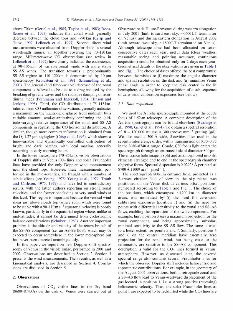
Fig. 2 presents the general aspect of spectra at8680–8740 A and a resolution R ¼ 120,000, stackedover and an entire acquisition sequence (August 1, 2002),for a full cycle of 15 exposure positions on Venus disk.Y-axis values, if multiplied by a factor 1000, represent,as an arbitrary flux unit, the number of photoelectronsco-added on 80 vertically summed CCD lines. X-axisnumbers are the detector pixel numbers. Differing fluxlevels reflect variable solar illumination (and possibly cloudtop albedo) from point to point, as well as possible fluxlosses due to pointing fluctuations near the limb andterminator.

The structure of the 5n3 band of 12C16O2 (assignednotation is 00051 in HITRAN database, Rothman et al.(2005)) is clearly apparent in Fig. 2. The observed spectrumshows about 30 P and R-branch lines with a folding back inthe R branch, a consequence of the decrease of rotationalconstant B0 with vibrational excitation (Campargue et al.,1994). The lines are detected with a typical unresolvedFWHM of 2.5 pixels and a S/N close to 50. Table 2indicates the list of 12C16O2 (hereafter referred to as CO2)lines identified in this study. At the observing resolution,some R-band lines in the blue end of the spectral range(lo8690 A) are only marginally well separated. Sinceradial velocity measurements require strong isolated andsymmetric lines, they were not used for wind determina-tion.

Fig. 3 shows a synthetic spectrum model of the 5n3band in Venus’ atmosphere, based on the spectralparameters of Campargue et al. (1994), and a simplereflecting-layer model using standard pressure–tempera-ture profile (Seiff et al., 1985). The reflecting layer wastaken at 65 km and the airmass to be 3. Here, we did notintend to precisely match the depth of the observed CO2

lines, as doing so in a meaningful manner would require theuse of a scattering code with detailed geometry. Thisreference spectrum, which indicates satisfactory agreementwith the observations in Fig. 2, will be used later toestimate the altitude level probed by the CO2 lines (seeSection 4.4).

No telluric lines have been identified within the8680–8740 A spectral range. Ten solar lines (Swennson etal., 1970), also reported in Table 2, were detected, and areidentified in Fig. 2 by a ‘~’ symbol followed by the solaratmospheric element (Mg I, Fe I, Si I, S I, Ba II or CN).Solar lines are broader (about 10 pixels) than Venus CO2

lines. As detailed below, three of these solar lines were usedfor wind measurements.

3. Doppler shift measurements

3.1. General method

Line positions in the various spectra (Venus CO2 lines,solar Fraunhofer lines, lamp spectra) were determinedfrom a standard Gaussian fit—the spectrum is locally fit tothe sum of a straight line and a Gaussian—using the IDLgaussfit procedure. Fitting molecular lines with a Gaussianfunction requires strong, isolated and quasi-symmetricalabsorption. Only a subset of CO2 visible lines (P(2) to P(40)and R(2) lines of 5n3 band), meet this requirement withinthe 8680–8740 A range. They are identified by a ‘*’ symbolin Table 2. Similarly, only three solar lines (8699.46,8717.83, and 8728.02 A) and four lamp lines (8679.58,8681.92, 8704.11 and 8705.57 A) turned out to be adequatefor Doppler shift measurements. The fit of the CO2

lines was performed on a 15-pixel interval, while forthe broader solar lines, the fit extended over 21 pixels(1 pixel ¼ 0.02928 A). An example of fit is shown in Fig. 4.Fit parameters, most importantly central position p and itsstandard deviation s, were obtained in pixel coordinates.Venus spectra were corrected for their instantaneoustopocentric velocity prior to fitting. For each line k, thedetermination of the 1s uncertainty attached to positionp(k) was performed following the method outlined inGoldstein et al. (1991) and Lellouch et al. (1994). Theresidual between the observed spectrum and its Gaussianfit is measured. Random noise at the level of this residual isgenerated and superimposed to the Gaussian model. Theresulting ‘‘noisy model’’ is refit, giving the line center at anew pixel position p0. The process is repeated 30 times witha new random noise distribution. The mean of p0–p is zero,and its standard deviation gives the 1s uncertainty s(k) onthe position p(k).

3.2. Absolute vs. relative spectral calibration

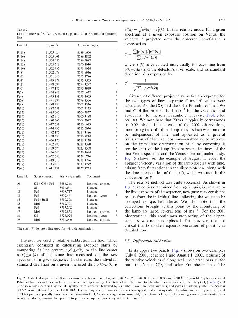
While lamp spectra provide, in principle, an absolutecalibration scale whose temporal variation can be mon-itored, the small number of lamp lines (four) made thisprocedure impractical. Although a dispersion law p ¼ f(l t)was established from a polynomial fit to the lamp linepositions, properly weighted according to their standarddeviation, this dispersion law turned out to be poorlydefined, especially in the long-wavelength part of thespectrum (l48710 A) given the absence of lamp linesthere. As a consequence, absolute wind velocities deter-mined in this manner were meaningless. This is illustratedin Fig. 5 on the example of the CO2 lines in one of theposition 3 spectra on August 1, 2002. The apparent velocityvaries by as much as 500m s�1 as a function of pixelnumber (i.e. as a function of line). This systematic error onindividual Doppler shift measurements cannot be removedwhen velocities from individual lines are weight-averagedto form the projected wind speed for the consideredexposure.

ARTICLE IN PRESS

Table 2

List of observed 12C16O2 5n3 band (top) and solar Fraunhofer (bottom)

lines

Line Id. s (cm�1) Air wavelength

R(18) 11505.424 8689.1660

R(16) 11505.001 8689.4852

R(14) 11504.455 8689.8982

R(12) 11503.786 8690.4030

R(10) 11502.993 8691.0024

R(8) 11502.078 8691.6936

R(6) 11501.040 8692.4786

R(4) 11499.879 8693.3563

R(2) 11498.594 8694.3277 *

R(0) 11497.187 8695.3919

P(2) 11494.846 8697.1628 *

P(4) 11493.131 8698.4603 *

P(6) 11491.294 8699.8506 *

P(8) 11489.334 8701.3346 *

P(10) 11487.251 8702.9123 *

P(12) 11485.045 8704.5837 *

P(14) 11482.717 8706.3488 *

P(16) 11480.266 8708.2077 *

P(18) 11477.691 8710.1613 *

P(20) 11474.995 8712.2076 *

P(22) 11472.176 8714.3486 *

P(24) 11469.234 8716.5834 *

P(26) 11466.170 8718.9128 *

P(28) 11462.983 8721.3370 *

P(30) 11459.674 8723.8558 *

P(32) 11456.242 8726.4694 *

P(34) 11452.688 8729.1776 *

P(36) 11449.012 8731.9796 *

P(38) 11445.213 8734.8782 *

P(40) 11441.291 8737.8725 *

Line Id. Solar element Air wavelength Comment

s0 SiI+CN+FeI 8686.368 Isolated, asymm.

s1 SI 8694.641 Blended

s2 FeI 8698.717 Blended

s3 FeI 8699.461 Isolated, symm. *

s4 FeI+BaII 8710.398 Blended

s5 MgI 8712.701 Blended

s6 FeI 8713.208 Blended

s7 MgI 8717.833 Isolated, asymm. *

s8 SiI 8728.024 Isolated, symm. *

s9 MgI 8736.040 Isolated, asymm.

The stars (*) denote a line used for wind determination.


Instead, we used a relative calibration method, whichessentially consisted in calculating Doppler shifts bycomparing fit line centers p(k)7s(k) to the line centerp1(k)7s1(k) of the same line measured on the first

spectrum of a given sequence. In this case, the individualstandard deviation on a given line pixel shift p(k)–p1(k) is

Fig. 2. A stacked sequence of 500-sec exposure spectra acquired August 1, 200

P-branch lines, as well as solar lines are visible. Each spectrum yields a total of

3 for solar lines identified by the ‘~’ symbol, with letter ‘‘s’’ followed by a nu

0.02928 A or 1009m s�1 per pixel at 8700 A. The three uppermost families of cu

7. Other points, especially those near the terminator (1, 4, 6), show a significan

seeing variability, causing the aperture to partly encompass regions beyond th

s0ðkÞ ¼ffiffiffiffiffiffiffiffiffiffiffiffiffiffiffiffiffiffiffiffiffiffiffiffiffiffiffis2ðkÞ þ s21ðkÞ

q. In this relative mode, for a given

spectrum at a given exposure position on Venus, thevelocity v0 projected onto the observer line-of-sight isexpressed as

v0 ¼

P½v0ðkÞ�

�½s02ðkÞ�P

½1�s02ðkÞ�

,

where v0(k) is calculated individually for each line fromp(k)–p1(k) and the detector’s pixel scale, and its standarddeviation s0 is expressed by

s0 ¼1ffiffiffiffiffiffiffiffiffiffiffiffiffiffiffiffiffiffiffiffiffiffiffiffiffiffiP

1�½s02ðkÞ�

q .

Given that different projected velocities are expected forthe two types of lines, separate v0 and s0 values werecalculated for the CO2 and the solar Fraunhofer lines. Wefind s0 of the order of 10–15m s�1 for the CO2 lines and20–30m s�1 for the solar Fraunhofer lines (see Table 3 forresults). We note here that 20m s�1 typically correspondsto 0.02 pixels. In the case of the 2002 observations,monitoring the drift of the lamp lines—which was found tobe independent of line, and appeared as a generaltranslation of the pixel position—enabled us to improveon the immediate determination of v0 by correcting itfor the shift of the lamp lines between the times of thefirst Venus spectrum and the Venus spectrum under study.Fig. 6 shows, on the example of August 1, 2002, theapparent velocity variation of the lamp spectra with time,arising from fluctuations in the dispersion law, along withthe time interpolation of this drift, which was used in thecorrection for v0.The relative method was quite successful. As shown in

Fig. 5, velocities determined from p(k)–p1(k), i.e. relative tothe first exposure of the sequence, now gave very consistentresults from the individual lines, allowing the values to beaveraged as specified above. We also note that thecorrections brought at this point by the monitoring ofthe lamp are large, several tens of m s�1. For the 2001observations, this continuous monitoring of the disper-sion law was not accomplished. This however, is a notcritical thanks to the frequent observation of point 1, asdetailed now.

3.3. Differential calibration

In its upper two panels, Fig. 7 shows on two examples(July 8, 2001, sequence 1 and August 1, 2002, sequence 3)the relative velocities v0 along with their error bars s0, forboth the Venus CO2 and solar Fraunhofer lines. The

2 at R ¼ 120,000 between 8680 and 8740 A. CO2-visible 5n3 R-branch and

26 individual Doppler-shift measurements for planetary CO2 (Table 2) and

mber. x-axis are pixel numbers, and y-axis an arbitrary intensity. Scale is

rves correspond, in decreasing order of continuum flux, to points 2, 3, and

t variability of continuum flux, due to pointing variations associated with

e terminator.

ARTICLE IN PRESS

Fig. 4. Example of Gaussian fits for a CO2 line (P(22) at 8714.35 A) and a solar Fraunhofer line (Si I at 8728.02 A). In this example, observations are from

July 8, 2001, and target point 1.

Fig. 3. Typical synthetic spectrum of CO2 5n3 band near 8700 A, using a reflecting layer at 65 km and a total airmass of 3.


velocities are plotted as a function of time, with the targetpoint numbers superimposed. Immediately apparent is thestrong drift of the v0 velocities for sequence 1, by almost

600m s�1 end to end. Such a drift would have beenmonitored and first-order corrected if a sufficient numberof lamp spectra had been acquired. For sequence 3, the

ARTICLE IN PRESS

Fig. 5. Illustration of absolute and relative calibration modes (see text, Section 3.2) on one example (point 3, sequence 3, August 1, 2002). x-axis is pixel

number and y-axis is line velocity in m s�1. Open squares: absolute velocities of all individual CO2 lines, shown with their error bars at their pixel position

on detector. The grossly inconsistent velocities from line to line are due to an inaccurate dispersion law. Filled triangles: relative velocities of each line, with

respect to first spectrum of the sequence. Relative velocities are now consistent for the various lines.

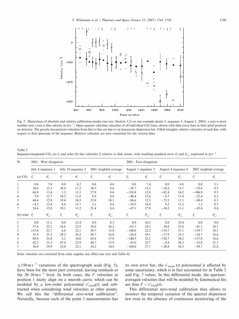
Table 3

Sequence-integrated CO2 (a) v0i and solar (b) line velocities s0i relative to disk center, with resulting standard error s0i and s0s;i, expressed in m s�1

Pt 2001—West elongation 2002—East elongation

July 8 sequence 1 July 10 sequence 2 2001 weighted average August 1 sequence 3 August 4 sequence 4 2002 weighted average

(a) CO2 v0i s0i v0i s0i v0i s0i v0i s0i v0i s0i v0i s0i

1 0.0 7.0 0.0 6.2 0.0 4.6 0.0 7.4 0.0 6.8 0.0 5.1

2 38.0 13.3 38.8 11.2 38.5 8.6 �58.7 13.2 �10.2 13.7 �35.4 9.5

3 66.8 13.4 1.2 11.1 27.9 8.6 �126.8 12.8 �82.4 14.2 �106.9 9.5

4 7.0 12.7 10.5 11.8 8.9 8.6 �40.4 12.6 �8.7 11.0 �22.4 8.3

5 44.4 12.8 19.4 16.5 35.0 10.1 �86.6 12.5 �75.5 11.1 �80.4 8.3

6 �4.2 13.4 8.6 11.7 3.1 8.8 �19.5 18.0 9.2 11.2 1.2 9.5

7 24.4 12.8 19.1 11.2 21.4 8.4 �67.1 17.9 �34.3 11.1 �43.4 9.4

(b) solar s0i s0s;i s0i s0s;i s0i s0s;i s0i s0s;i s0i s0s;i s0i s0s;i

1 0.0 11.1 0.0 12.4 0.0 8.3 0.0 10.2 0.0 19.4 0.0 9.0

2 57.6 22.1 16.6 23.8 38.6 16.2 �63.3 18.3 34.6 33.8 �41.1 16.1

3 115.4 22.7 6.8 22.1 59.7 15.8 �180.0 22.2 �119.7 31.1 �159.7 18.1

4 31.8 21.3 29.2 24.2 30.7 16.0 �26.9 19.1 �17.9 33.5 �24.7 16.6

5 89.0 21.0 5.1 34.0 65.8 17.9 �140.5 22.1 �128.7 34.2 �137.0 18.6

6 42.2 21.3 47.9 23.9 44.7 15.9 �43.6 25.7 �8.8 38.2 �32.8 21.3

7 36.0 19.9 32.0 22.1 34.2 14.8 �104.0 27.1 +20.8 36.5 �59.7 21.8

Solar velocities are corrected from solar angular size effect (see text and Table 4).


7150m s�1 variations of the spectrograph scale (Fig. 5),have been for the most part corrected, leaving residuals atthe 20–30m s�1 level. In both cases, the v0 velocities atposition 1 nicely align on a smooth curve, which can bemodeled by a low-order polynomial v0trend(t) and sub-tracted when considering wind velocities at other points.We call this the ‘‘differential zero-wind calibration’’.Naturally, because each of the point 1 measurements has

its own error bar, the v0trend (t) polynomial is affected bysome uncertainty, which is in fact accounted for in Table 3and Fig. 7 values. In this differential mode, the aperture-averaged velocities that will be modeled by kinematical fitsare thus v0 � v0trendðtÞ.This differential zero-wind calibration thus allows to

monitor the temporal variation of the spectral dispersionlaw even in the absence of continuous monitoring of the

ARTICLE IN PRESS

Fig. 7. Relative velocities measured sequences 1 (July 8, 2001) and 3 (August 1, 2002), plotted as a function of time. The target points at Venus are

indicated. Open squares: CO2 lines. Filled triangles: Solar Fraunhofer lines. In the two top panels, the solid and dashed lines show a polynomial fit of the

velocities at point 1 determined independently for the CO2 and the solar lines. In the bottom two panels, this polynomial fit was subtracted from the

individual measurements, providing ‘‘differential’’ winds (see text).

Fig. 6. Absolute drift of the spectral dispersion law, as monitored by the translation of Th–Ne lamp lines, during measurements of August 1, 2002. x-axis

is time after 0 h UT, y-axis is shift in m s�1. Open squares indicate lamp measurements with their error bars. Variations up to 7150m s�1 with respect to

first lamp exposure are seen and can be monitored. These are interpolated to correct the pixel scale of Venus spectra (located in time by the triangles).

Stability improves after �2 h of operation.



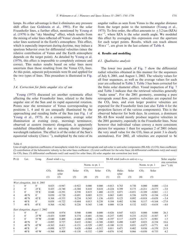
lamps. Its other advantage is that it eliminates any pressureshift effect (see Goldstein et al., 1991). For the solarFraunhofer lines, a further effect, mentioned by Young etal. (1979) is the ‘‘sky blending’’ effect, which results fromthe mixing of solar lines reflected off Venus’ clouds with thesolar lines scattered in the Earth’s atmosphere. This effect,which is especially important during daytime, may induce aspurious behavior even for differential velocities (since therelative contribution of Venus and the Earth atmospheredepends on the target point). As detailed by Young et al.(1979), this effect is impossible to completely estimate andcorrect. This makes results based on solar lines moreuncertain than those resulting from the Venus CO2 lines.At this point, separate polynomials were fit and applied forthe two types of lines. This procedure is illustrated in Fig.7.

3.4. Correction for finite angular size of sun

Young (1975) discussed yet another systematic effectaffecting the solar Fraunhofer lines, related to the finiteangular size of the Sun and its rapid equatorial rotation.Points near the terminator of Venus (corresponding topositions 1, 4 and 6) are unequally illuminated by theapproaching and receding limbs of the Sun (see Fig. 1 ofYoung et al., 1975). As a consequence, average solarillumination at evening (resp., morning) terminator,observed at eastern (western) elongation, is apparentlyredshifted (blueshifted) due to missing shorter (longer)wavelength radiation. The effect is of the order of the Sun’sequatorial velocity (2 km s�1), multiplied by the ratio of its

Table 4

Line-of-sight projection coefficients of mesospheric winds for a zonal retrograd

(2) contribution of the heliocentric velocity to the solar lines coefficient ; (3) tot

for CO2 lines; (5) differential coefficients rsz(i) and ssas(i) for solar lines; (6) s

Pt (i) Lat. Long. Zonal wind� veq

Norm. to pt

CO2 Helio.

solar

Solar CO2 So

(1) (2) (3) (4) (5

West elongation, July 8, 2001

1 01 01 0.025 �0.947 �0.922 0.000 0

2 01 251E 0.435 �0.740 �0.304 0.410 0

3 01 551E 0.848 �0.291 0.558 0.823 1

4 401N 01 0.030 �0.720 �0.691 0.005 0

5 401N 451E 0.568 �0.335 0.234 0.543 1

6 401S 01 0.038 �0.722 �0.684 0.013 0

7 401S 451E 0.568 �0.342 0.226 0.543 1

East elongation, August 1, 2002

1 01 01 �0.034 0.974 0.940 0.000 0

2 01 251W �0.435 0.809 0.374 �0.401 �0

3 01 551W �0.840 0.400 �0.440 �0.806 �1

4 401N 01 �0.095 0.727 0.632 �0.061 �0

5 401N 451W �0.563 0.411 �0.151 �0.529 �1

6 401S 01 �0.098 0.727 0.628 �0.064 �0

7 401S 451W �0.566 0.408 �0.158 �0.532 �1

angular radius as seen from Venus to the angular distancefrom the target point to the terminator (Young et al.,1975). To first order, the effect amounts to 73.2 tan (SZA)m s�1, where SZA is the solar zenith angle. We modeledthis effect by averaging this expression over the aperturefor each target points. Results, which can reach almost30m s�1, are given in the last column of Table 4.

4. Results and modelling

4.1. Qualitative analysis

The lower two panels of Fig. 7 show the differentialradial velocities obtained in this manner for the sequencesof July 8, 2001, and August 1, 2002. The velocity values forall four sequences, as well as the average values for eachyear are collected in Table 3. Table 3 has been corrected forthe finite solar diameter effect. Visual inspection of Fig. 7and Table 3 indicate that the retrieved velocities generally‘‘make sense’’. For the 2001 geometry, assuming a pureretrograde zonal flow, positive velocities are expected forthe CO2 lines, and even larger positive velocities areexpected for the Fraunhofer lines (see also Table 4 for theprojection factors of the various components). This is theobserved behavior for both days. In contrast, a dominantSS–AS flow would mostly produce negative velocities inthe 2001 geometry, especially in the Fraunhofer lines. Notehowever that individual values convey a more consistentpicture for sequence 1 than for sequence 2 of 2001 (wherethe very small value for the CO2 lines at point 3 is clearlyanomalous). For 2002, all velocities are expected to be

e and sub-solar to anti-solar components (SS-AS): (1) CO2 lines coefficient;

al coefficient for the solar lines; (4) differential coefficients rsz(i) and ssas(i)

olar angular size correction (see text)

SS-AS wind (sub-s.to anti-s)� vter Solar angular

size correction

(m s�1) (6). 1 Norm. to pt. 1

lar CO2 Helio.

solar

Solar CO2 Solar

) (1) (2) (3) (4) (5)

.000 �0.013 0.763 0.750 0.000 0.000 �12.6

.618 �0.224 0.399 0.175 �0.211 �0.575 �3.8

.480 �0.122 0.071 �0.051 �0.109 �0.801 �1.1

.231 0.065 0.491 0.556 0.078 �0.194 �15.4

.156 �0.031 0.123 0.092 �0.018 �0.658 �3.4

.238 0.104 0.482 0.586 0.117 �0.164 �27.0

.148 0.008 0.124 0.132 0.021 �0.618 �4.0

.000 �0.026 0.847 0.821 0.000 0.000 26.3

.566 �0.257 0.492 0.235 �0.232 �0.587 4.7

.380 �0.197 0.117 �0.079 �0.171 �0.901 1.5

.308 �0.003 0.490 0.487 0.023 -0.334 18.6

.092 �0.100 0.151 0.051 �0.075 �0.771 4.0

.312 0.011 0.471 0.482 0.036 �0.339 21.9

.099 �0.076 0.142 0.066 �0.050 -0.755 4.2


negative (regardless of whether the flow is dominantlyzonal or SS–AS), and once again to be more negative forthe Fraunhofer lines than for the CO2 lines. Reassuringly,this is what is observed, although again, a few measure-ments do not fit well in the general picture, especially thevery low and nominally positive velocity of the Fraunhoferlines at point 7 in sequence 4. Is is also instructive toconsider mean velocities for each year (i.e. averages forsequences 1+2, and 3+4, respectively). For both types oflines, the values, particularly at points 3, 5, 7 are morenegative in 2002 than they are positive in 2001.This qualitatively suggests that a minor SS–AS componentdoes superimpose on the dominant retrograde zonalflow. The significance of this result needs, however, tobe assessed. At this point, results are encouraging andwarrant the kinematical modeling presented in the nextsection.

4.2. Kinematical modelling

The final velocities, relative to disk center, and correctedfor the various effects discussed above, were then modeledusing a kinematical model for the circulation in Venus’mesosphere. Both a zonal and SS–AS components wereintroduced. Following previous studies, notably resultsfrom CO millimeter-wave observations (Lellouch et al.,1994), the zonal flow was generally described as solid-bodyrotation, i.e. in the form vzonal (l) ¼ �veq� cos l, where l islatitude. The SS–AS flow was assumed to be axisymme-trical about the SS–AS line, with a maximum cross-terminator velocity vter. Again, following previous studies(Goldstein et al., 1991), we usually adopted a vSSAS ¼

vter� (1�|901�SZA|/901) dependence, where SZA is thesolar zenithal angle. We refer below to this kind of modelas ‘‘model 1’’. As detailed later, other functional depen-dences for the zonal and SSAS flow were tested, butwithout success. Projection factors for heliocentric andgeocentric line-of-sight were calculated with the help of ageometrical model (Lellouch et al., 1994). Explicit expres-sions for these projections factors are best found inGoldstein (1989). Because the instrumental aperture coversa significant fraction of Venus’ disk, the projection factorswere calculated over a fine grid of points and averaged overthe beam (Venus’ disk was partitioned into a 120(radius)� 360 (azimuth) grid). The total, beam-averagedvelocity towards the observer at point i can finally bewritten as

v0mod;i ¼ rszðiÞ � veq þ ssasðiÞ � vter,

where rsz(i) and ssas(i) are the beam-averaged projectioncoefficients—including the latitudinal and/or SZA depen-dences indicated above. These projection coefficients aresummarized in Table 4, for the CO2 lines (label ‘‘CO2’’ inTable 4) and for the solar Fraunhofer lines (label ‘‘Solar’’).For the latter, Table 4 separately indicates the contributionof the heliocentric velocity (label ‘‘Helio. solar’’) to thetotal projection factor. The slightly non-zero values of the

projection factors for the CO2 lines at beam positions 1, 4,and 6 are due to the large beam size. Table 4 also containsthe ‘‘differential projection coefficients’’ between thevarious points and point 1. Examination of these differ-ential projection factors supports the qualitative discus-sions of the previous sections. The last column of Table 4gives the value of the finite solar size effect, which has beensubtracted to the solar lines velocities in Table 3.The measured velocities are finally compared to the

above kinematical model (in which rsz(i) and ssas(i) arenow the differential projection coefficients) and best fit issought by varying veq and vter. As a matter of fact, andgiven the qualitative inspection of the results, we con-sidered (i) zonal only models and (ii) two-componentmodel. veq (or veq and vter) were varied until best agreementto the measurements was achieved, and the acceptableparameter space was defined from classical w2 analysis.Specifically, we calculated the reduced w2, w2red, and

its square root, S ¼ffiffiffiffiffiffiffiffiw2red

q, where

w2red ¼1

ðNobs �NparÞ

Xi

ðv0i � v0mod;iÞ2

s02i,

where Nobs ¼ 6 and Npar ¼ 1 for pure zonal flow andNpar ¼ 2 for both zonal and SS–AS flows. Best fit wasachieved for S ¼ Smin, and the acceptable parameterspace was defined by the requirement that SpSmin�

ffiffiffiffiffiffiffiffiffiffiffiffiffiffiffiffiffiffiffiffiffiffiffiffiffiffiffiffiffiffiffiffiffiffiffiffiffiffiffiffiffi1þ 4=ðNobs �NparÞ

p(at 2s) or SpSmin�ffiffiffiffiffiffiffiffiffiffiffiffiffiffiffiffiffiffiffiffiffiffiffiffiffiffiffiffiffiffiffiffiffiffiffiffiffiffiffiffiffi

1þ 9=ðNobs �NparÞp

(at 3 s). A good fit is typically

indicated by Smin�1. A more quantitative estimate of thegoodness-of-fit is given by Q(n, w2) ¼ 1–P(n/2, w2/2), whereP is the incomplete gamma function, n ¼ Nobs�Npar is thenumber of degrees of freedom, and w2 ¼ nS2 is the chi-square (Press et al., 1992). Q gives the probability that theobserved w2 exceeds the value w2 by chance even for acorrect model. The expected value for a moderately goodfit is Q ¼ 0.5. Much lower values indicate that the model isunacceptable, the error bars are underestimated, or theerror bars are not normally distributed. Q values largerthan 0.5 generally indicate that the error bars areoverestimated.

4.3. Modelling results

Table 5 contains the results of the kinematical modeling,for the solar and CO2 lines, for the four observing datesseparately and for the averages over 2001 and 2002, andusing either a zonal component only, or both a zonal and aSS–AS flows. This modeling generally confirms thequalitative examination of Table 4. Starting with a singlezonal component and the CO2 lines, all days individuallyindicate a significant, yet quite variable zonal flow.Equatorial velocities range from 25 to 155m s�1, with atypical 2s error bar of 15–35m s�1. The average value overthe veq is about 80m s�1. With the error bars objectively

determined as explained previously, S ¼ffiffiffiffiffiffiffiffiw2red

qvaries from

ARTICLE IN PRESS

Table 5

Kinematical fits of CO2 lines and solar lines velocities with (i) a pure zonal retrograde flow (ii) a two-component model, characterized by equatorial

velocity veq of zonal wind, and cross-terminator velocity vter of SS-AS wind

Sequence CO2 wind field Solar lines wind field

Smin Q veq (m s�1) vter (m s�1) Smin Q veq (m s�1) vter (m s�1)

West elongation (2001)

1 zonal 0.72 0.76 74.8715.0 1.24 0.17 67.1722.5

zonal+ssas 0.69 0.75 70.0715.0 �44.775. 1.24 0.19 0.765. �116.7130

2 zonal 1.49 4.9� 10�2 25.1722.0 1.07 0.33 16.4714.0

zonal+ssas 1.62 3.3� 10�3 20.0727.5 �40.7155. 1.15 0.26 0.752.5 �307112

1+2 zonal 1.33 0.11 47.3719.0 1.33 0.12 44.7718.0

zonal+ssas 1.39 0.10 43.0722.5 �37.797.5 1.29 0.15 0.742.5 �78787.5

East elongation (2002)

3 zonal 1.21 0.20 155.7727.5 0.64 0.84 120.7712.5

zonal+ssas 1.30 0.15 169.752.5 �60.777.5 0.68 0.76 147.772.5 �367100

4 zonal 1.65 1.8� 10�2 94.5734.5 1.71 1.2� 10�2 60.9751.0

zonal+ssas 1.74 1.6� 10�2 111.760. �86.7207.5 1.72 1.9� 10�2 168.7125. �150.7190

3+4 zonal 1.78 7.3� 10�3 123.0727.0 1.41 7.7� 10�2 101.7723.5

zonal+ssas 1.93 4.9� 10�3 134.750. �53.7200. 1.48 6.7� 10�2 154.7120. �727172.5

Combined measurements (2001+2002)

zonal 2.60 1.8� 10�11 82.8727.5 2.04 3.5� 10�6 67.2721.5

zonal+ssas 2.45 3.6� 10�9 80.725. 84.7105. 1.51 1.1� 10�2 70.715.0 40722.5

Error bar gives 2s acceptable domain (m s�1).


�0.7 (‘‘too good fit’’) to 1.7 (‘‘bad fit’’), a behavior we areunable to completely explain. However, the Q probabilitiesare never vanishingly small (i.e. they generally remainabove �10�2) on individual days so that the models may bedeemed acceptable. Quite remarkably, zonal winds re-trieved from the Fraunhofer lines are on a day-to-day basisvery consistent with those inferred from CO2 (Fig. 8(a)).Unlike this is a fortunate coincidence, this suggests that theFraunhofer lines are not strongly affected by the blendingeffect described in Young et al. (1979), perhaps resultingfrom our choice to discard any observations with obvioushaze scattering. Weight-averaging the results over theindividual days, the zonal wind equatorial velocity is77711m s�1 from the CO2 lines and 7378m s�1 from thesolar Fraunhofer lines.

As detailed in Table 5, the inclusion of the subsolar toantisolar component does not improve fit quality

(theffiffiffiffiffiffiffiffiw2red

qnever diminishes significantly), nor bring new

information when individual days are considered. This is infact not too surprising, considering (i) the admittedly largeerror bars of many of our measurements and (ii) the factthat on a given date, the projection coefficients (see Table4) for the SS–AS flow are either small (o0.26 for the CO2

lines) or strongly correlated (2002) or anti-correlated (2001)with those for the zonal flow (Fraunhofer lines). As aresult, the influence of the SS–AS flow on the observedwind velocities is either small or similar to that of the zonalflow (i.e. enhancing or compensating it in a similar mannerat all points). Thus error bars on vter are always very large

and vter is statistically indistinguishable from zero. In thecase of the solar lines, the acceptable domain appears as anelongated ellipse in the (veq, vter) space with ‘‘positive’’(2001) or ‘‘negative’’ (2002) orientation (i.e. constrainingeither veq�vter or veq+vter). Within error bars, retrievedzonal wind equatorial velocities are consistent with thevalues they take in the 1-component model.In search of fitting improvement, we tested other

functional dependences for the zonal and SS-AS flow. Inparticular, solid-body rotation is not the only regime thathas been observed at cloud tops. For example, a fairlyconstant velocity with latitude has been observed byGalileo in 1990, while velocities increasing with latitudeover [0,7451] in jet-like structures have been reported byMariner 10 in 1974 and Pioneer Venus in 1980 and 1982(see Fig. 3 of Gierasch et al., 1997). We therefore testedadditional models in which the zonal velocity was eitherconstant with latitude l (model 2), or increasing as 1/cos(l)(model 3; although such a dependence cannot obviouslyhold up to high latitudes, this is unimportant because ourmeasurements do not sample latitudes4551). Finally, wealso tried a quadratic dependence of the SS-AS flow,namely vSSAS ¼ vter� (1�[|901�SZA|/901]2), in combina-tion with a cos(l) dependence for the zonal flow (model 4).None of these additional models, however, proved to bemore successful than the original model. Smin values wereeither largely unchanged, or significantly worse. In parti-cular, fits were always systematically worse for model 3compared to model 1, tending to exclude the presence ofstrong mid-latitude jets in 2001 and 2002.

ARTICLE IN PRESS

Fig. 8. (a) Kinematical fit to CO2 lines (open squares) and solar lines

(open triangles) with 2s acceptable domain for a pure zonal retrograde

flow, illustrating the variability of equatorial velocity with time (see Table

5 for details). Velocities in m s�1 are plotted vs. sequence number (1: 2001-

07-08; 2: 2001-07-10; 3: 2002-08-01; 4: 2002-08-04). (b) 2s solution domain

in the (veq, vter) space for fitting of the grand ensemble of 2001+2002 solar

Fraunhofer lines data.


Coming back to model 1, we finally combined data from2001 and 2002, analyzing the entire data set with a singlemodel (12 independent observation points). This exercisemight be viewed as of limited interest given the highlyvariable character of the zonal flow we infer (and the fact,in particular, that some of the solution domains forindividual days are mutually exclusive). Nonetheless, bydoing so, we are trying to infer the ‘‘mean atmosphericregime’’ over the entire period of our measurements. In thiscase, we find that the ensemble of CO2 line measurementsleads to an equatorial velocity veq ¼ 83727m s�1 for azonal only model, and veq ¼ 80725m s�1, vter ¼ 847105m s�1 for the 2-component model (2s error bars).Not surprisingly in view of the above remarks, the fit is

poor (Smin�2.5, Qo10�8). For the Fraunhofer lines, thecorresponding values are veq ¼ 67721m s�1 (Smin ¼ 2.04),or veq ¼ 70715m s�1, vter ¼ 40722m s�1 (Smin ¼ 1.51),respectively. This is the only situation where considering aSS–AS flow allows a significant improvement of fit quality.In fact, with the exception of the 2-component model of theFraunhofer lines, the very low Q probabilities indicate thatthe associated models simply do not fit the data. For theFraunhofer lines, the domain in the (veq, vter) space isshown in Fig. 8(b). These lines suggest that the SS–AS flowis detected (and still direct, as opposed to retrograde) at thealtitude level sampled by our measurements. We do,however, regard this conclusion as tentative given theabove caveat on temporal variability and the fact that themodels do not match the CO2 lines.

4.4. Altitude determination

Visible light is reflected and scattered off Venus cloudtops. Analysis of early polarisation data (Hansen andHovenier, 1974) indicated a cloud top altitude (opticaldepth of unity) of 65–70 km. The UV features (365 nm),from which most of the wind measurements have beenobtained, are probably formed just below the level wherethe UV vertical optical depth is unity (Gierasch et al.,1997). Based on a detailed analysis of Pioneer Venus OCPPdata at 270, 365, 550 and 935 nm, this level is about40mbar pressure and 70 km altitude (Kawabata et al.,1980). More precisely, the Kawabata et al. (1980) modelconsists of a main cloud, with particle size of 1.05 mm,underlain by and partly mixed with a haze with �0.2 mmparticle size. The optical depth of the haze is about 0.6 at40mbar, and varies roughly as l�1.7. At the wavelength ofour observations (870 nm), this gives t ¼ 0.27 at 70 km,and the t ¼ 1 level due to haze would be reached at 64 km.For the main cloud, the dependence of extinction withwavelength is much smaller. We thus estimate that thesolar Fraunhofer lines near 870 nm probe the atmosphere(373) km below the UV features, i.e. near 67 km. This isprobably less than one scale height apart, so that smalldifferences in the dynamical regime are expected.For the CO2 lines formed on Venus, the probed altitude

is a little higher because the CO2 lines progressively absorbsolar radiation above the cloud tops. To estimate thealtitude relevant to our measurements, we used the simpleradiative transfer model that led to the reference syntheticspectrum of Fig. 3. We then imposed a line-of-sight windprofile, decreasing linearly from 100m s�1 at the cloud topto 0m s�1 at some higher level, and recalculated thesynthetic spectrum with the Doppler shift resulting fromthis wind profile included (level by level, in the absorptioncoefficient). This produced shifted and asymmetric lineprofiles, whose apparent Doppler shift was measured fromthe reference synthetic spectrum. Varying the 0m s�1 level(from 10 to 40 km above the reflecting level), we found thatthe apparent Doppler shift corresponded to the wind speed772 km (or about two scale heights) above the reflecting


layer. We conclude that the wind measurements using theCO2 lines refer to a layer that is approximately 7 kilometersabove the one associated with the solar Fraunhofer lines,i.e. near typically 74 km altitude.

5. Discussion and conclusions

Our measurements using the CO2 lines indicate that afew kilometers above the cloud tops, zonal retrogradewinds are present with significant equatorial velocities(�75m s�1 in average) and very large (450m s�1) short-term (days) variability. This is generally consistent with theresults of Traub and Carleton (1975, 1979). Based on8708 A CO2 line measurements, Traub and Carleton (1979)found a mean equatorial velocity of 85710m s�1 (con-sistent with the earlier results of Traub and Carleton(1975), based on one CO2 line and one Fraunhofer line), onwhich a 40714m s�1 variation superimposes with a periodof 4.370.2 days. While our measurements do not haveenough temporal sampling to establish whether thevariability we are observing is periodic, the similarity ofour results to those of the previous authors reinforces thecredibility of wind measurements at visible wavelengths.We note however, that while the mean values reported byTraub and Carleton and in this work are similar to themean zonal wind velocities deduced from the UV features(�90m s�1 at Equator), the latter are characterized by amuch weaker variability (715m s�1) than the ground-based measurements.

Mean zonal wind velocities inferred from the Fraunhoferlines, which probe the �67 km range, are fully consistenton a day-to-day basis with those measured from CO2,sampling the atmosphere near 74 km. This suggests thatonce the systematic effects (blending effect, and finite sizeof the Sun effect) are properly handled, the Fraunhoferlines can also be used for wind measurements. In thisrespect, our results disagree with those of Young (1975)and Young et al. (1979), who after correcting for theseeffects in the early data of Richardson (1958) as well as indata of their own, derived essentially zero wind velocities(e.g. 10733, 27716, 26736m s�1) from the solar Fraun-hofer lines. We note that their results are somewhatdifficult to understand if, as suggested above, the solarFraunhofer lines probe the atmosphere a few kilometersbelow the UV features. In the present study, the generalagreement between the wind values inferred from the twotypes of lines supports the case for a negligible wind shearover two scale heights near clouds top, although the resultwould have been obviously strengthened by the availabilityof simultaneous wind measurements from cloud tracking.

Temporal variability of the zonal flow has been seen inthe CO mm-wave observations (see review in Lellouch etal., 1997), which probe the 95–105 km range. Most recentevidence for this was obtained by Clancy et al. (2005) whofound large variations of wind velocities over periods ofhours to years, including variations larger than 50m s�1

over hourly timescales. This variability is generally

interpreted as due to variable gravity–wave activity, sincethe latter are thought to be responsible for the overalldecrease of the zonal wind with altitude through momen-tum deposition upon wave breaking. Our results, alongwith those of Traub and Carleton, suggest that the samemechanism may be at work throughout most of Venus’mesosphere (75–105 km).Considering all our data together, we tentatively detect

the SS–AS flow at �67 km in the Fraunhofer lines, with across-terminator velocity of 40722.5m s�1. This value issimilar to what was measured in 1991 by Lellouch et al.(1994) from CO mm-wave observations, namely vter ¼

40715m s�1 at 95 km. Unlike the zonal retrograde flow,previous measurements suggest that the SS–AS flow israther stable. If real, our detection would indicate apenetration of the SS–AS flow into the lower mesospherewithout strong attenuation from its upper mesospherevalue, a challenging result for thermospheric models(Bougher et al., 1986). However, for the various reasonsdiscussed above, our results on the SS–AS flow must betaken prudently. In addition, the UV markings, whichprobe the atmosphere at a similar level, have not revealedthe presence of the SS-AS component. In any event, ourmeasurements do not confirm the tentative reinterpretationby Goldstein (1989) of the Betz et al. (1976) 13CO2 10-mmmeasurements in terms of an anti-solar to sub-solar flow(AS–SS) of 3576m s�1 at 7475 km. (Note that from masscontinuity considerations, Goldstein (1989) stressed thatsuch a high speed at this level was difficult to sustain.) Theproblem of the altitude and speed of the return branch ofthe thermospheric circulation thus remains unresolved.Besides the numerous systematic effects described in this

paper, the precision of the wind measurements fromDoppler shifts is S/N-limited. In these respects, progressmay be achieved by using more novel high-resolution visiblespectrometers. In particular, the HARPS instrument onESO 3.60m telescope and the newest SOPHIE spectrometeron OHP 1.93m telescope are equipped with a high precision(o1m s�1) internal wavelength calibration system usingTh–Ar or I2 cells. Long-slit spectroscopy, such as thatafforded by the VLT/UVES cross-dispersed echelle spectro-meter, has the advantage of providing an instantaneousone-dimensional image of the wind Doppler shift, e.g. alongthe Polar axis or the Equator, enabling a direct determina-tion of the latitudinal dependence of the zonal flow andfacilitating the search for wave and tidal structures.The VIRTIS instrument (Drossart et al., 2007) onboard

Venus Express has started to address the problem ofmesospheric dynamics from extensive mapping and mon-itoring of the temperature above the clouds from CO2 4.3-and 15-mm spectroscopy over a nominal mission period of2 Venusian days (�500 Earth days). Wind measurements atcloud tops are also routinely performed from UV tracking,and comparison with concomitant observations based onthe Doppler technique used here will be very useful. Moregenerally, in the absence of direct wind measurementsabove cloud level by Venus Express, ground-based


Doppler spectroscopy in visible, thermal (10-mm) and mm-wave radiation will remain a complementary approach,necessary to apprehend the full complexity of the Venus’middle atmosphere circulation and its temporal variations.

Acknowledgments

The authors wish to thank Programme National dePlanetologie (CNES/INSU) for its 2-years support of thisprogram. The paper is dedicated to Jean-Paul Bretagne whocontributed to observations in 2002, and passed away inFebruary 2006. As mentioned to us by J.-L. Bertaux and A.Hauchecorne after acceptance of this paper, a differentialrotation between the cloud tops and the overlying gas wouldinduce a splitting of the CO2 lines as seen by the observer.This effect, which does not affect the solar Fraunhofer lines,would complicate the analysis of the CO2 lines. However,this effect disappears when no vertical shear is present, whichis the situation indicated by our observations.

References

Betz, A.L., Johnson, M.A., Mclaren, R.A., Sutton, E.C., 1976. Hetero-

dyne detection of CO2 emission lines and wind velocities in the

atmosphere of Venus. Astrophys. J. (Lett.) 208, 41–44.

Bougher, S.W., Dickinson, R.E., Ridley, E.C., Roble, R.G., Nagy, A.F.,

Cravens, T.E., 1986. Venus mesosphere and thermosphere, II: global

circulation, temperature, and density variations. Icarus 68, 284–312.

Bougher, S.W., Alexander, M.J., Mayr, H.G., 1997. Upper atmosphere

dynamics: global circulation and gravity waves. In: Bougher, S.W.,

Hunten, D.M., Phillips, R.J. (Eds.), Venus II. University of Arizona

Press, Tucson, pp. 259–291.

Burnage, R., Gillet, D., Kohler, D., Meunier, J.P., 1990. Le Spectrometre

Aurelie, Observatoire de Haute Provence, CNRS (Internal document).

Campargue, A., Charvat, A., Permogorov, D., 1994. Absolute intensity

measurement of CO2 overtone transitions in the near-infrared. Chem.

Phys. Lett. 223, 567–572.

Clancy, R.T., Sandor, B.J., Moriarty-Schieven, G., 2005. Submillimeter

observations of global variations in chemistry and dynamics in the

Venus mesosphere. Bull. Am. Astron. Soc. 37 (3), 741, #54.04.

Crisp, D., Meadows, V.S., Bezard, B., de Bergh, C., Maillard, J.P., Mills,

F.P., 1996. Ground-based near-infrared observations of the Venus

nightside: 1.27-mm O2(a1Dg) airglow from the upper atmosphere. J.

Geophys. Res. 101 (E2), 4459–4577.

Crisp, D., Titov, D., 1997. The thermal balance of the Venus atmosphere.

In: Bougher, S.W., Hunten, D.M., Phillips, R.J. (Eds.), Venus II.

University of Arizona Press, Tucson, pp. 353–384.

Drossart, P., Piccioni, G., Adriani, A., Angrilli, F., Arnold, G., Baines,

K.H., Bellucci, G., Benkhoff, J., Bezard, B., Bibring, J.-P., et al., 2007.

Scientific goals for the observation of Venus by VIRTIS on ESA/

Venus Express mission, Planetary and Space Science, this issue,

doi:10.1016/j.pss.2007.01.003.

Gierasch, P.J., Goody, R.M., Young, R.E., Crisp, D., Edwards, C., Kahn,

R., Rider, D., Del Genio, A., Greeley, R., Hou, A., Leovy, C.B.,

McCleese, D., Newman, M., 1997. The general circulation of the

Venus atmosphere: an assessment. In: Bougher, S.W., Hunten, D.M.,

Phillips, R.J. (Eds.), Venus II. University of Arizona Press, Tucson,

pp. 459–500.

Gillet, D., Burnage, R., Kohler, D., Lacroix, D., Adrianzyk, G., Baietto,

J.C., Berger, J.P., Goillandeau, M., Guillaume, C., Joly, C., Meunier,

J.P., Rimbaud, G., Vin, A., 1994. AURELIE: the high resolution

spectrometer of the Haute-Provence Observatory. Astron. Astrophys.

Suppl. 108, 181.

Goldstein, J.J., 1989. Absolute wind velocities in the lower thermosphere

of Venus USINF infrared Heterodyne Spectroscopy. Ph.D. Thesis,

University of Pennsylvania, Philadelphia. NASA CR-4290, May 1990.

Goldstein, J.J., Mumma, M.J., Kostiuk, T., Deming, D., Espenak, F.,

Zipoy, D., 1991. Absolute wind velocities in the lower thermosphere of

Venus using infrared heterodyne spectroscopy. Icarus 94, 45–63.

Hansen, J.E., Hovenier, J.W., 1974. Interpretation of the polarization of

Venus. J. Atmos. Sci. 31, 1137–1160.

Hinson, D.P., Jenkins, J.M., 1995. Magellan radio occultation measure-

ments of atmospheric waves on Venus. Icarus 114, 310–327.

Kawabata, K., Coffeen, D.L., Hansen, J.E., Lane, W.A., Sato, M., Travis,

L.D., 1980. Cloud and haze properties from pioneer Venus polari-

metry. J. Geophys. Res. 85, 8129–8140.

Lellouch, E., Goldstein, J.J., Rosenqvist, J., Bougher, S.W., Paubert, G.,

1994. Global circulation, thermal structure and carbon monoxide

distribution in Venus’ mesosphere in 1991. Icarus 110, 315–339.

Lellouch, E., Clancy, T., Crisp, D., Kliore, A.J., Titov, D., Bougher, S.W.,

1997. Monitoring of mesospheric structure and dynamics. In: Bougher,

S.W., Hunten, D.M., Phillips, R.J. (Eds.), Venus II. University of

Arizona Press, Tucson, pp. 295–324.

Oertel, D., et al., 1985. Infrared spectroscopy of Venus from Venera-15

and Venera-16. Adv. Space. Res. 5 (9), 25–36.

Pechmann, J.B., Ingersoll, A.P., 1984. Thermal tides in the atmosphere of

Venus: comparison of model results with observations. J. Atmos. Sci.

41, 3290–3313.

Press, W.H., Flannery, B.P., Teukolsky, S.A., Vetterling, W.T., 1992.

Numerical Recipes. Cambridge University Press, New York, NY, USA.

Richardson, R.S., 1958. Spectroscopic observation of Venus for rotation

made at Mount Wilson in 1956. Publ. Astron. Soc. Pacific 70, 251–260.

Roos-Serote, M., et al., 1995. The thermal structure and dynamics of the

atmosphere of Venus between 70 and 90 km from the Galileo-NIMS

spectra. Icarus 114, 300–309.

Rothman, L.S., Jacquemart, D., Barbe, A., Chris Benner, D., Birk, M.,

Brown, L.R., Carleer, M.R., Chackerian Jr., C., Chance, K., Dana, V.,

Devi, V.M., Flaud, J.-M., Gamache, R.R., Goldman, A., Hartmann,

J.-M., Jucks, K.W., Maki, A.G., Mandin, J.-Y., Massie, S.T., Orphal,

J., Perrin, A., Rinsland, C.P., Smith, M.A.H., Tennyson, J.,

Tolchenov, R.N., Toth, R.A., Vander Auwera, J., Varanasi, P.,

Wagner, G., 2005. The HITRAN 2004 Molecular Spectroscopic

Database. J. Quant. Spectrosc. Radiat. Transfer 96, 139–204.

Schmuelling, F., Goldstein, J., Kostiuk, T., Hewagama, T., Zipoy, D.,

2000. High precision wind measurements in the upper Venus atmo-

sphere. Bull. Am. Astron. Soc. 32 (64.05), 1121.

Schubert, G., 1983. General circulation and the dynamical state of the

Venus atmosphere. In: Hunten, D.M., et al. (Eds.), Venus. University

of Arizona Press, Tucson, pp. 681–765.

Seiff, A., Schofield, J.T., Kliore, A.J., Taylor, F.W., Limaye, S.S.,

Revercomb, H.E., Sromovsky, L.A., Kerzhanovitch, V.V., Moroz,

V.I., Marov, M.YA., 1985. Models of the structure of the atmosphere

of Venus from the surface to 100 kilometers altitude. Adv. Space Res. 5

(11), 3–58.

Swennson, J.W., Benedict, W.S., Delbouille, L., Roland, G., 1970. The

Solar Spectrum from l7498 to l12016. Memoires de la Societe Royale

des Sciences de Liege, Hors Serie (5), Liege, Belgique.

Taylor, F.W., et al., 1983. The thermal balance of the middle and upper

atmosphere of Venus. In: Hunten, D.M., et al. (Eds.), Venus.

University of Arizona Press, Tucson, pp. 650–680.

Toigo, A., Gierasch, P.J., Smith, M.D., 1994. High-resolution cloud

feature tracking on Venus by Galileo. Icarus 109 (2), 318–336.

Traub, W.A., Carleton, N.P., 1975. Spectroscopic observations of winds

on Venus. J. Atmos. Sci. 32, 1045–1059.

Traub, W.A., Carleton, N.P., 1979. Retrograde winds on Venus—possible

periodic variations. Astrophys. J. 227, 329–333.

Young, A.T., 1975. Is the four-day rotation of Venus illusory? Icarus 24,

1–10.

Young, A.T., Schorn, R.A., Young, L.D.G., Crisp, D., 1979. Spectro-

scopic observations of winds on Venus, I—technique and data

reduction. Icarus 38, 435–450.

dx.doi.org/10.1016/j.pss.2007.01.003

new wind measurements in venus’ lower mesosphere … · new wind measurements in venus’ lower...

Documents