Citation: Hirt, C, S.J. Claessens, T. Fecher, M. Kuhn, R. Pail, M. Rexer (2013), New ultra-high resolution picture of 1 Earth's gravity field, Geophysical Research Letters, Vol 40, doi: 10.1002/grl.50838. 2

3

New ultra-high resolution picture of Earth’s gravity field 4

5 Christian Hirt1*, Sten Claessens1, Thomas Fecher2, Michael Kuhn1, Roland Pail2, Moritz Rexer1, 2 6 1 Western Australian Centre for Geodesy, Curtin University, Perth, Australia 7 2 Institute for Astronomical and Physical Geodesy, Technical University Munich, Germany 8 * E-mail: c.hirt@curtin.edu.au 9 10 Abstract 11 We provide an unprecedented ultra-high resolution picture of Earth’s gravity over all continents 12 and numerous islands within ± 60 degree latitude. This is achieved through augmentation of new 13 satellite and terrestrial gravity with topography data, and use of massive parallel computation 14 techniques, delivering local detail at ~200 m spatial resolution. As such, our work is the first-of-15 its-kind to model gravity at unprecedented fine scales yet with near-global coverage. The new 16 picture of Earth’s gravity encompasses a suite of gridded estimates of gravity accelerations, 17 radial and horizontal field components and quasigeoid heights at over 3 billion points covering 18 80% of Earth’s land masses. We identify new candidate locations of extreme gravity signals, 19 suggesting that the CODATA standard for peak-to-peak variations in free-fall gravity is too low 20 by about 40%. The new models are beneficial for a wide range of scientific and engineering 21 applications and freely available to the public. 22 23 Keywords 24 Earth’s gravity field, gravity, quasigeoid, vertical deflections, ultra-high resolution 25 26 1 Introduction 27 28 Precise knowledge of the Earth’s gravity field structure with high resolution is essential for a 29 range of disciplines, as diverse as exploration and potential field geophysics [Jakoby and Smilde, 30 2009], climate and sea level change research [Rummel, 2012], surveying and engineering 31 [Featherstone, 2008] and inertial navigation [Grejner-Brzezinska and Wang, 1998]. While there 32 is a strong scientific interest to model Earth’s gravity field with ever-increasing detail, the 33 resolution of today’s gravity models remains limited to spatial scales of mostly 2-10 km globally 34 [Pavlis et al., 2012; Balmino et al., 2012], which is insufficient for local gravity field 35 applications such as modelling of water flow for hydro-engineering, inertial navigation or in-situ 36 reduction of geophysical gravity field surveys. Up until now, gravity models with sub-km 37 resolution are unavailable for large parts of our planet. 38 39 Here we provide an unprecedented ultra-high resolution view of five components of Earth’s 40 gravity field over all continents, coastal zones and numerous islands within ±60 degree latitude. 41 This is achieved through augmentation of new satellite and terrestrial gravity with topography 42 data [e.g., Hirt et al. 2010] and use of massive parallel computation techniques, delivering local 43 detail at 7.2 arc-seconds (~200 m in North-South direction) spatial resolution (Section 2). As 44 such, our work is the first-of-its-kind to model gravity at ultra-fine scales yet with near-global 45 coverage. The new picture of Earth’s gravity encompasses a suite of gridded estimates of gravity 46

accelerations, radial and horizontal field components and quasigeoid heights at over 3 billion 47 points covering 80% of Earth’s land masses and 99.7% of populated areas (Section 3, 4). This 48 considerably extends our current knowledge of the gravity field. The gridded estimates are 49 beneficial for a range of scientific and engineering applications (Section 5) and freely available 50 to the public. Electronic supplementary materials are available providing full detail on the 51 methods applied in this study. 52 53 2 Data and Methods 54 55 Our ultra-high resolution picture of Earth’s gravity field is a combined solution based on the 56 three key constituents GOCE/GRACE satellite gravity (providing the spatial scales of ~10000 57 down to ~100 km), EGM2008 (~100 to ~10 km) and topographic gravity, i.e., the gravitational 58 effect implied by a high-pass filtered terrain model (scales of ~10 km to ~250 m), 59 60 Regarding the satellite component, we use the latest satellite-measured gravity data (release 61 GOCE-TIM4) from the European Space Agency’s GOCE satellite [Drinkwater et al., 2003; Pail 62 et al., 2011], parameterized as coefficients of a spherical harmonic series expansion, that 63 currently provides the highest-resolution picture of Earth’s gravity ever obtained from a space 64 gravity sensor. Resolving gravity field features at spatial scales as short as 80-100 km, GOCE 65 confers new gravity field knowledge, most notably over poorly surveyed regions of Africa, 66 South America and Asia [Pail et al., 2011]. 67 68

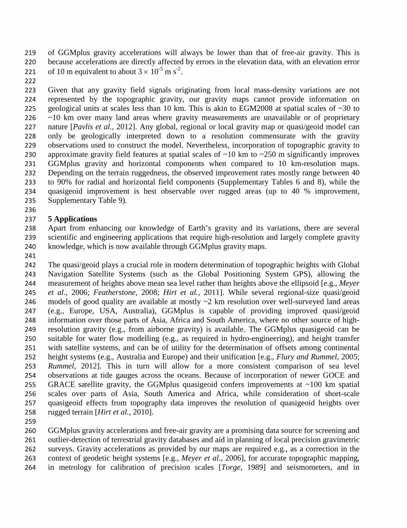
69 Figure 1. Relative contribution of GOCE/GRACE data per spherical harmonic coefficient in the combination with 70 EGM2008 data (in percent) for the degrees 0 to 250 71 72 Compared to pure GOCE models, complementary GRACE satellite gravity [Mayer Guerr et al., 73 2010] are superior in the spectral range up to degrees 70-80 [Pail et al., 2010]. Therefore, first a 74 combined satellite-only combined solution based on full normal equations of GRACE (up to 75 degree 180) and GOCE (up to degree 250) is computed [see, e.g., Pail et al., 2010]. The 76 GRACE/GOCE combination is then merged with EGM2008 [Pavlis et al., 2012] using the 77 EGM2008 coefficients as pseudo-observations. Since for EGM2008 only the error variances are 78 available, the corresponding normal equations have diagonal structure. In our combination, 79 GRACE/GOCE data have dominant influence in the spectral band of harmonic degrees 0 to 180 80 with EGM2008 information taking over in the spectral range 200 to 2190, leaving the main 81 spectral range of transition from GRACE/GOCE to EGM2008 in spectral band of degrees 181 to 82

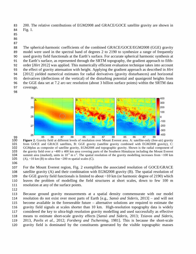
200. The relative contributions of EGM2008 and GRACE/GOCE satellite gravity are shown in 83 Fig. 1. 84 85 86 87 The spherical-harmonic coefficients of the combined GRACE/GOCE/EGM2008 (GGE) gravity 88 model were used in the spectral band of degrees 2 to 2190 to synthesize a range of frequently 89 used gravity field functionals at the Earth’s surface. For accurate spherical harmonic synthesis at 90 the Earth’s surface, as represented through the SRTM topography, the gradient approach to fifth-91 order [Hirt 2012] was applied. This numerically efficient evaluation technique takes into account 92 the effect of gravity attenuation with height. Applying the gradient approach as described in Hirt 93 [2012] yielded numerical estimates for radial derivatives (gravity disturbances) and horizontal 94 derivatives (deflections of the vertical) of the disturbing potential and quasigeoid heights from 95 the GGE data set at 7.2 arc-sec resolution (about 3 billion surface points) within the SRTM data 96 coverage. 97 98

99 Figure 2. Gravity field at different levels of resolution over Mount Everest area. A: satellite-only (free-air) gravity 100 from GOCE and GRACE satellites, B: GGE gravity (satellite gravity combined with EGM2008 gravity), C: 101 GGMplus as composite of satellite gravity, EGM2008 and topographic gravity. Shown is the radial component of 102 the gravity field over a ~400 x 400 km area covering parts of the Southern Himalayas including the Mount Everest 103 summit area (marked), units in 10-5 m s-2. The spatial resolution of the gravity modelling increases from ~100 km 104 (A), ~10 km (B) to ultra-fine ~200 m spatial scales (C). 105 106 For the Mount Everest region, Fig. 2 exemplifies the associated resolution of GOCE/GRACE 107 satellite gravity (A) and their combination with EGM2008 gravity (B). The spatial resolution of 108 the GGE gravity field functionals is limited to about ~10 km (or harmonic degree of 2190) which 109 leaves the problem of modelling the field structures at short scales, down to few 100 m 110 resolution at any of the surface points. 111 112 Because ground gravity measurements at a spatial density commensurate with our model 113 resolution do not exist over most parts of Earth [e.g., Sansò and Sideris, 2013] – and will not 114 become available in the foreseeable future – alternative solutions are required to estimate the 115 gravity field signals at scales shorter than 10 km. High-resolution topography data is widely 116 considered the key to ultra-high resolution gravity modelling and used successfully as effective 117 means to estimate short-scale gravity effects [Sansò and Sideris, 2013; Tziavos and Sideris, 118 2013, Pavlis et al., 2012; Forsberg and Tscherning, 1981]. This is because the short-scale 119 gravity field is dominated by the constituents generated by the visible topographic masses 120

[Forsberg and Tscherning, 1981]. However, forward estimation of the short-scale gravity field 121 constituents from elevation models near-globally at ultra-high (few 100 metres) resolution is 122 computationally demanding. Yet we have accomplished this challenge for the first time through 123 advanced computational resources. 124 125 Massive parallelization and the use of Western Australia’s iVEC/Epic supercomputing facility 126 allowed us to convert topography from the Shuttle Radar Topography Mission (SRTM), cf. 127 Jarvis et al. [2008] – along with bathymetric information along coastlines [Becker et al., 2009] – 128 to topographic gravity at 7.2 arc-sec resolution everywhere on Earth between ± 60° latitude with 129 SRTM data available. Based on non-parallelized standard computation techniques, the 130 calculation of topographic gravity effects would have taken an estimated 20 years, which is why 131 previous efforts were restricted to regional areas [Kuhn et al., 2009; Hirt, 2012]. 132 133 The conversion of topography to topographic gravity is based on the residual terrain modelling 134 technique [Forsberg, 1984], with the topography high-pass filtered through subtraction of a 135 spherical harmonic reference surface (of degree and order 2160) prior to the forward-modelling. 136 We treated the ocean water masses and those of the major inland water bodies (Great Lakes, 137 Baikal, Caspian Sea) using a combination of residual terrain modelling with the concept of rock-138 equivalent topography [Hirt, 2013], whereby the water masses were ‘compressed’ to layers 139 equivalent to topographic rock. These procedures yield short-scale topographic gravity that is 140 suitable for augmentation of degree-2190 spherical harmonic gravity models beyond their 141 associated 10 km resolution, cf. Hirt [2010; 2013]. The topographic gravity is based on a mass-142 density assumption of 2670 kg m-3 and provides the spatial scales of ~10 km to ~250 m, which is 143 complementary to the GGE gravity (spatial scales from ~10000 km to ~10 km). 144 145 3 Results 146 147 Addition of both components (GGE and topographic gravity) result in the ultra-high resolution 148 model GGMplus (Global Gravity Model, with plus indicating the leap in resolution over 149 previous 10 km resolution global gravity models). The modelled gravity field components and 150 their descriptive statistics are reported in Table 1. 151 152 Table 1. Descriptive statistics of the GGMplus model components calculated at 3,062,677,383 land and 153 near-costal points within ± 60° geographic latitude. RMS is the root-mean-square of the component. 154 Gravity model component Min Max RMS Unit Gravity Free-fall acceleration 976392 981974 980133 10-5 m s-2 Radial component -456 714 48.0 10-5 m s-2 Horizontal components North-South -108 94 6.9 arc-sec East-West -83 79 6.8 arc-sec Total (magnitude) 0 109 9.4 arc-sec Quasigeoid -99.26 86.60 29.91 m 155 This world-first ultra-high resolution modelling over most of Earth’s land areas delivered us the 156 expected gravity signatures of small-scale topographic features – such as mountain peaks and 157 valleys – which are otherwise masked in 10 km resolution models. This adds much local detail to 158 the gravity maps (compare Figs. 2B and 2C) and yields a spectrally more complete and accurate 159 description of the gravity field [e.g., Hirt, 2012]. 160

Table 2. Candidate locations for extreme values of Earth’s gravity field 161 Gravity component Minimum/

Maximum Latitude/ Longitude

Geographic feature/ location

Gravity acceleration 9.76392 m s-2 -9.12°/ -77.60° Huascarán, Peru 9.83366 m s-2 86.71°/61.29° *Arctic Sea Radial component -456 × 10-5 m s-2 29.71°/95.36° Gandengxiang, China 714 × 10-5 m s-2 10.83°/-73.69° Pico Cristóbal Colón, Columbia Horizontal component+

109 arc-sec 28.45°/84.13° ~10 km South of Annapurna II, Nepal

Quasigeoid -106.59 m 4.71°/78.79° *Laccadive Sea, South of Sri Lanka

86.60 m -8.40°/147.35° Puncak Trikora, Papua, Indonesia * offshore area, value estimated without topographic gravity using GGE-only (10 km resolution, also see 162 electronic supplement) 163 + total component computed as magnitude from the North-South and East-West components 164 165

166 Figure 3. Candidate locations of some extreme signals in Earth’s gravity in the Andes (A,B) and Himalaya regions 167 (C,D). Top: Topography (A) and free-fall gravity accelerations (B) over the Huascarán region (Peru), where 168 GGMplus gravity accelerations are as small as ~9.764 m s-2 (B). Bottom: Topography (C) and GGMplus total 169 horizontal field component (D) over the Annapurna II region (Nepal). The gravitational attraction of the Annapurna 170 II masses is expected to cause an extreme slope of the quasi/geoid with respect to the Earth ellipsoid of up to ~109 171 arc-seconds (D). 172

Our gridded estimates portray the subtle variations of gravity (Fig. 3) which are known to depend 173 on factors such as location, height and presence of mass-density anomalies. GGMplus reveals a 174 candidate location for the minimum gravity acceleration on Earth: the Nevado Huascarán summit 175 (Peru) with an estimated acceleration of 9.76392 m s-2 (Fig 3A, 3B, and Table 2). A candidate 176 location for Earth’s maximum gravity acceleration was identified - outside the SRTM area, based 177 on GGE-only – in the Arctic sea with an estimated 9.83366 m s-2. This suggests a variation range 178 (peak-to-peak variation) for gravity accelerations on Earth of about ~0.07 m s-2, or 0.7 %, which 179 is about 40 % larger than the variation range of 0.5 % implied by standard models based on a 180 rotating mass-ellipsoid (gravity accelerations are 9.7803 m s-2 (equator) 9.8322 m s-2 (poles) on 181 the mass-ellipsoid, cf. Moritz [2000]). So far such a simplified model is also used by the 182 Committee on Data for Science and Technology (CODATA) to estimate the variation range in 183 free-fall acceleration on Earth [Mohr and Taylor, 2005]. However, due to the inhomogeneous 184 structure of Earth, presence of topographic masses, and decay of gravity with height the actual 185 variations in free-fall accelerations are ~40% larger at the Earth’s surface (Table 2). 186 187 GGMplus free-air gravity – the radial component of Earth’s gravity field – varies within a range 188 of ~0.011 m s-2 (~0.1% of gravity accelerations) with its minimum value of –456 × 10-5 m s-2 189 located in China and its maximum of 714 × 10-5 m s-2 expected for the Pico Cristóbal Colón 190 summit in Colombia. The higher variability of gravity accelerations over free-air gravity reflects 191 the well-known fact that gravity accelerations include the gravitational attraction and centrifugal 192 effect due to Earth rotation. 193 194 The horizontal components of the gravitational field describe in approximation the North-South 195 and East-West inclination of the quasi/geoid with respect to the reference ellipsoid. The variation 196 range of the horizontal field components (also known as deflections of the vertical) is about ~200 197 arc-seconds in North South, and ~160 arc-seconds in East-West, respectively (Table 1). 198 GGMplus reveals a candidate location for Earth’s largest deflection of the vertical: about 10 km 199 South of Annapurna II, Nepal, the plumb line is expected to deviate from the ellipsoid normal by 200 an angle as large as ~109 arc-seconds (Fig. 3C and 3D). This translates into a most extreme 201 quasi/geoid slope of about 0.5 m over 1 km. 202 203 4 Model evaluation 204 205 We have comprehensively compared GGMplus gravity field maps with in-situ (direct) 206 observations of Earth’s gravity field from gravimetry, astronomy, and surveying (see electronic 207 supplementary materials). Over well-surveyed areas of North America, Europe and Australia, 208 the comparisons suggest an accuracy level for free-air gravity and gravity accelerations of ~5 × 209 10-5 m s-2, for horizontal field components of about 1 arc-second, and for quasigeoid heights of 210 0.1 m or better. 211 212 Despite the improvements conferred by recent satellite gravity to our model, the GGMplus 213 accuracy deteriorates by a factor of ~3 to ~5 over Asia, Africa and South America which are 214 regions with limited or very limited ground gravity data availability. Comparisons suggest a 215 decrease in accuracy down to ~20 × 10-5 m s-2 for gravity, ~5 arc-seconds for horizontal field 216 components, and ~0.3 m for quasigeoid heights. The reduced accuracy estimates mainly reflect 217 the limited availability of gravity observations at spatial scales of ~100 to ~10 km. The accuracy 218

of GGMplus gravity accelerations will always be lower than that of free-air gravity. This is 219 because accelerations are directly affected by errors in the elevation data, with an elevation error 220 of 10 m equivalent to about 3 × 10-5 m s-2. 221 222 Given that any gravity field signals originating from local mass-density variations are not 223 represented by the topographic gravity, our gravity maps cannot provide information on 224 geological units at scales less than 10 km. This is akin to EGM2008 at spatial scales of ~30 to 225 ~10 km over many land areas where gravity measurements are unavailable or of proprietary 226 nature [Pavlis et al., 2012]. Any global, regional or local gravity map or quasi/geoid model can 227 only be geologically interpreted down to a resolution commensurate with the gravity 228 observations used to construct the model. Nevertheless, incorporation of topographic gravity to 229 approximate gravity field features at spatial scales of ~10 km to ~250 m significantly improves 230 GGMplus gravity and horizontal components when compared to 10 km-resolution maps. 231 Depending on the terrain ruggedness, the observed improvement rates mostly range between 40 232 to 90% for radial and horizontal field components (Supplementary Tables 6 and 8), while the 233 quasigeoid improvement is best observable over rugged areas (up to 40 % improvement, 234 Supplementary Table 9). 235 236 5 Applications 237 Apart from enhancing our knowledge of Earth’s gravity and its variations, there are several 238 scientific and engineering applications that require high-resolution and largely complete gravity 239 knowledge, which is now available through GGMplus gravity maps. 240 241 The quasi/geoid plays a crucial role in modern determination of topographic heights with Global 242 Navigation Satellite Systems (such as the Global Positioning System GPS), allowing the 243 measurement of heights above mean sea level rather than heights above the ellipsoid [e.g., Meyer 244 et al., 2006; Featherstone, 2008; Hirt et al., 2011]. While several regional-size quasi/geoid 245 models of good quality are available at mostly ~2 km resolution over well-surveyed land areas 246 (e.g., Europe, USA, Australia), GGMplus is capable of providing improved quasi/geoid 247 information over those parts of Asia, Africa and South America, where no other source of high-248 resolution gravity (e.g., from airborne gravity) is available. The GGMplus quasigeoid can be 249 suitable for water flow modelling (e.g., as required in hydro-engineering), and height transfer 250 with satellite systems, and can be of utility for the determination of offsets among continental 251 height systems (e.g., Australia and Europe) and their unification [e.g., Flury and Rummel, 2005; 252 Rummel, 2012]. This in turn will allow for a more consistent comparison of sea level 253 observations at tide gauges across the oceans. Because of incorporation of newer GOCE and 254 GRACE satellite gravity, the GGMplus quasigeoid confers improvements at ~100 km spatial 255 scales over parts of Asia, South America and Africa, while consideration of short-scale 256 quasigeoid effects from topography data improves the resolution of quasigeoid heights over 257 rugged terrain [Hirt et al., 2010]. 258 259 GGMplus gravity accelerations and free-air gravity are a promising data source for screening and 260 outlier-detection of terrestrial gravity databases and aid in planning of local precision gravimetric 261 surveys. Gravity accelerations as provided by our maps are required e.g., as a correction in the 262 context of geodetic height systems [e.g., Meyer et al., 2006], for accurate topographic mapping, 263 in metrology for calibration of precision scales [Torge, 1989] and seismometers, and in 264

observational astronomy for meteorological corrections [Corbard et al., 2013]. For geophysics 265 and the exploration industry, GGMplus may prove beneficial as novel data source for in-situ 266 reduction of detailed gravimetric surveys, revealing locations of interest for mineral prospectivity 267 without the need to calculate and apply further rather time-consuming reductions [Jakoby and 268 Smilde, 2009] Finally, horizontal field components are required to correct the impact of the 269 Earth’s irregular gravity field, e.g., for inertial navigation at or near the Earth’s surface [Grejner-270 Brzezinska and Wang, 1998], or in the context of civil engineering (e.g., precision surveys for 271 tunnel alignment), Featherstone and Rüeger [2000]. All of these applications require spectrally 272 most complete information on the gravity field. 273 274 6 Conclusions 275 276 GGMplus provides the most complete description of Earth’s gravity at ultra-high resolution and 277 near-global coverage to date. This confers immediate benefits to many applications in 278 engineering, exploration, astronomy, surveying, and potential field geophysics. While GGMplus 279 provides moderate additional information (because of the ultra-high resolution short-scale 280 modelling) over areas with dense coverage of gravity stations (e.g., North America, Europe, 281 Australia), significant improvements are provided over areas with sparse ground gravity 282 coverage (e.g., Asia, Africa, South America). For the latter regions, GGMplus provides for the 283 first time a complete coverage with gravity at ultra-high spatial resolution, thus providing 284 scientific aid to many developing countries. In addition, GGMplus provides crucial information 285 to revise current standards for the maximum range of free-fall gravity accelerations over the 286 Earth’s surface. The computerized GGMplus gravity field maps are freely available for science, 287 education and industry via and http://ddfe.curtin.edu.au/gravitymodels/GGMplus. 288 289 Acknowledgements We are grateful to the Australian Research Council for funding 290 (DP120102441). This work was made feasible through using advanced computational resources 291 of the iVEC/Epic supercomputing facility (Perth, Western Australia). We thank all developers 292 and providers of data used in this study. Full methods, and detailed evaluation results are 293 available in the electronic supplementary information, and information on data access via the 294 project’s website http://geodesy.curtin.edu.au/research/models/GGMplus. 295 296 References 297 Balmino, G., N. Vales, S. Bonvalot and A. Briais (2012), Spherical harmonic modelling to ultra-high degree of 298

Bouguer and isostatic anomalies, J. Geod., 86(7), 499-520, doi: 10.1007/s00190-011-0533-4. 299 Becker, J.J., D.T. Sandwell, W.H.F. Smith, J. Braud, B. Binder, J. Depner, D. Fabre, J. Factor, S. Ingalls, S-H. Kim, 300

R. Ladner, K. Marks, S. Nelson, A. Pharaoh, R. Trimmer, J. Von Rosenberg, G. Wallace and P. Weatherall 301 (2009), Global Bathymetry and Elevation Data at 30 Arc Seconds Resolution: SRTM30_PLUS, Marine 302 Geod., 32(4), 355-371. 303

Corbard T., F. Morand, F. Laclarex, R. Ikhlef, and M. Meftah (2013), On the importance of astronomical refraction 304 for modern Solar astrometric measurements, Astr. Astrophy., April 2, 2013. 305

Drinkwater, M.R., R. Floberghagen, R. Haagmans, D. Muzi, and A. Popescu (2003), GOCE: ESA's first Earth 306 Explorer Core mission, In (eds. Beutler, G.B., M.R. Drinkwater, R. Rummel, and R. von Steiger), Earth 307 Gravity Field from Space - from Sensors to Earth Sciences. In the Space Sciences Series of ISSI, Vol. 18, 308 419-432, Kluwer Academic Publishers, Dordrecht, Netherlands ISBN: 1-4020-1408-2. 309

Featherstone W.E. (2008), GNSS-based heighting in Australia: current, emerging and future issues, J. Spat. Sci. 53, 310 115-133. 311

Featherstone W.E., and J.M. Rüeger (2000), The importance of using deviations of the vertical for the reduction of 312 survey data to a geocentric datum, Australian Surveyor, 45, 46-61. 313

Flury, J., and R. Rummel (2006), Future satellite gravimetry for geodesy, Earth Moon Plan. 94, 13-29. 314 doi:10.1007/s11038-005-3756-7 315

Forsberg R., and C.C. Tscherning (1981), The use of height data in gravity field approximation by collocation, J. 316 Geophys. Res, 86(B9), 7843-7854. 317

Forsberg, R. (1984), A study of terrain reductions, density anomalies and geophysical inversion methods in gravity 318 field modelling, Report 355, Department of Geodetic Science and Surveying, Ohio State University, 319 Columbus. 320

Grejner-Brzezinska, D.A., and J. Wang (1998), Gravity modeling for high-accuracy GPS/INS integration, 321 Navigation, 45, 3, 209-220. 322

Hirt, C. (2010), Prediction of vertical deflections from high-degree spherical harmonic synthesis and residual terrain 323 model data, J. Geod., 84 (3), 179-190. doi:10.1007/s00190-009-0354-x 324

Hirt, C., W.E. Featherstone and U. Marti (2010), Combining EGM2008 and SRTM/DTM2006.0 residual terrain 325 model data to improve quasigeoid computations in mountainous areas devoid of gravity data, J. Geod., 84(9): 326 557-567, DOI: 10.1007/s00190-010-0395-1.. 327

Hirt C., Schmitz M., Feldmann-Westendorff U., Wübbena G., Jahn C.-H., and Seeber G. (2011), Mutual validation 328 of GNSS height measurements from high-precision geometric-astronomical levelling, GPS Solutions, 15(2), 329 149-159, DOI 10.1007/s10291-010-0179-3. 330

Hirt, C. (2012), Efficient and accurate high-degree spherical harmonic synthesis of gravity field functionals at the 331 Earth's surface using the gradient approach, J. Geod., 86(9), 729-744, doi: 10.1007/s00190-012-0550-y. 332

Hirt, C. (2013), RTM gravity forward-modeling using topography/bathymetry data to improve high-degree global 333 geopotential models in the coastal zone, Marine Geod., 36(2):1-20, doi:10.1080/01490419.2013.779334. 334

Jacoby, W., and P.L. Smilde (2009), Gravity interpretation, Springer, Berlin, Heidelberg. 335 Jarvis, A., H.I. Reuter, A. Nelson, and E. Guevara (2008), Hole-filled SRTM for the globe Version 4, Available from 336

the CGIAR-SXI SRTM 90m database. Available at: http://srtm.csi.cgiar.org. 337 Kuhn, M., W.E. Featherstone, and J.F. Kirby (2009), Complete spherical Bouguer gravity anomalies over Australia, 338

Australian J. Earth Sci., 56, 213-223. 339 Mohr P. J., and B.N. Taylor (2005), CODATA recommended values of the fundamental physical constants: 2002, 340

Rev. Mod. Phys. 77 (Jan 2005). 341 Moritz, H. (2000), Geodetic Reference System 1980. J. Geod., 74, 128-140. 342 Meyer T.H., D.R. Roman, and D.B. Zilkoski (2006), What Does Height Really Mean? Part IV: GPS Heighting. 343

Surveying Land Inf. Sci. 66, 165-183. 344 Mayer-Gürr, T., E. Kurtenbach, and A. Eicker (2010), ITG-Grace2010 Gravity Field Model. URL: 345

http://www.igg.uni-bonn.de/apmg/index.php?id=itg-grace2010, 2010. 346 Pail, R., Goiginger, H., W.-D. Schuh, E. Höck, J.M. Brockmann, T. Fecher, T. Gruber, T. Mayer-Gürr, J. Kusche, A. 347

Jäggi, and D Rieser (2010), Combined satellite gravity field model GOCO01S derived from GOCE and 348 GRACE, Geophys. Res. Lett. 37, L20314, doi: 10.1029/2010GL044906. 349

Pail, R., S. Bruinsma, F. Migliaccio, C. Förste, H. Goiginger, W.-D. Schuh, E. Höck, M. Reguzzoni, J.M. 350 Brockmann, O. Abrikosov, M. Veicherts, T. Fecher, R. Mayrhofer, I. Krasbutter, F. Sansò, and C.C. 351 Tscherning (2011), First GOCE gravity field models derived by three different approaches, J Geod., 85(11), 352 819-843, doi: 10.1007/s00190-011-0467-x. 353

Pavlis N.K., S.A. Holmes, S.C. Kenyon, and J.K. Factor (2012), The development and evaluation of the Earth 354 Gravitational Model 2008 (EGM2008), J. Geophys. Res., 117, B04406, doi:10.1029/2011JB008916. 355

Rummel, R. (2012), Height unification using GOCE. J. Geod. Sci. 2, 355-362. 356 Sansò F., and M.G. Sideris (2013), The Local Modelling of the Gravity Field: The Terrain Effects. Lecture Notes in 357

Earth System Sciences 110, 169, Springer, Berlin Heidelberg. 358 Tziavos, I.N., and M.G. Sideris (2013), Topographic Reductions in Gravity and Geoid Modeling. Lecture Notes in 359

Earth System Sciences 110, 337-400, Springer, Berlin Heidelberg. 360 Torge W. (1989), Gravimetry, de Gruyter, Berlin, New York. 361 362 363 364 365 366 367 368 369

Electronic supplementary material for 370 371

New ultra-high resolution picture of Earth’s gravity field 372 373

Christian Hirt1*, Sten Claessens1, Thomas Fecher2, Michael Kuhn1, Roland Pail2, Moritz Rexer1,2 374 375

1 Western Australian Centre for Geodesy, Curtin University, Perth, Australia 376 2 Institute for Astronomical and Physical Geodesy, Technical University Munich, Germany 377 378

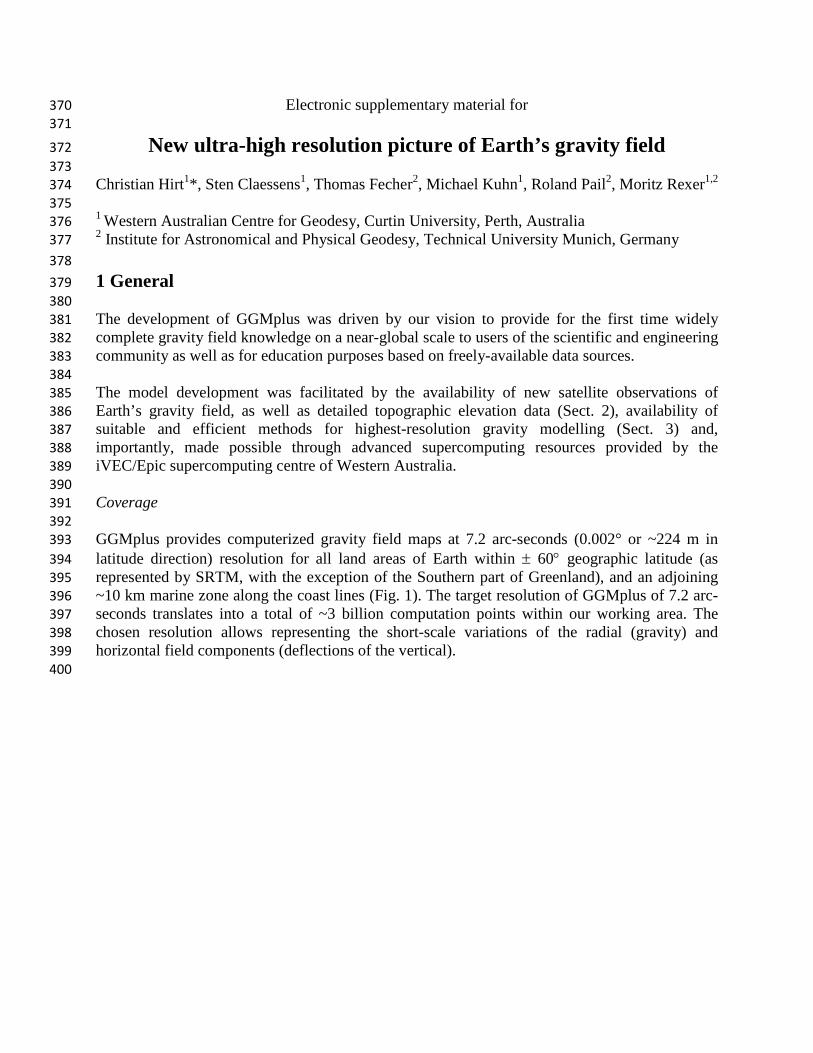
1 General 379 380 The development of GGMplus was driven by our vision to provide for the first time widely 381 complete gravity field knowledge on a near-global scale to users of the scientific and engineering 382 community as well as for education purposes based on freely-available data sources. 383 384 The model development was facilitated by the availability of new satellite observations of 385 Earth’s gravity field, as well as detailed topographic elevation data (Sect. 2), availability of 386 suitable and efficient methods for highest-resolution gravity modelling (Sect. 3) and, 387 importantly, made possible through advanced supercomputing resources provided by the 388 iVEC/Epic supercomputing centre of Western Australia. 389 390 Coverage 391 392 GGMplus provides computerized gravity field maps at 7.2 arc-seconds (0.002° or ~224 m in 393 latitude direction) resolution for all land areas of Earth within ± 60° geographic latitude (as 394 represented by SRTM, with the exception of the Southern part of Greenland), and an adjoining 395 ~10 km marine zone along the coast lines (Fig. 1). The target resolution of GGMplus of 7.2 arc-396 seconds translates into a total of ~3 billion computation points within our working area. The 397 chosen resolution allows representing the short-scale variations of the radial (gravity) and 398 horizontal field components (deflections of the vertical). 399 400

401 Figure 1. Coverage of GGMplus. Shown are mean values of the radial component of the gravity 402 field over land and near-coastal areas between ± 60° geographic latitude. 403 404 Technical definitions 405 406 The five gravity field functionals provided by GGMplus are 407 408

• Free-fall gravity accelerations (i.e. gravitational plus centrifugal accelerations) 409 • Gravity disturbances (radial derivatives of the disturbing potential), denoted as radial 410

component of the gravity field in the manuscript 411 • North-South deflection of the vertical in Helmert definition (latitudinal derivative of the 412

disturbing potential), denoted as horizontal component of the gravity field in the 413 manuscript 414

• East-West deflection of the vertical in Helmert definition (longitudinal derivative of the 415 disturbing potential), denoted as horizontal component of the gravity field in the 416 manuscript 417

• and Molodenski quasigeoid heights. 418 419

All quantities are given at the Earth’s surface as defined through the SRTM (Shuttle Radar 420 Topography Mission) topography. Users wishing to use geoid heights instead of quasigeoid 421 heights can do so by applying standard conversion as described, e.g., Rapp [1997]. 422

423

2 Data sets used 424 425 A complete list of data sets used for the development of GGMplus is given in Table 1. The use of 426 these data is further detailed in Section 3. 427 428 Table 1. Data sets used for the development of GGMplus 429 Dataset Ressource Citation

GRACE satellite gravity model ITG2010s

http://icgem.gfz-potsdam.de/ICGEM Mayer-Gürr et al. [2010]

GOCE-TIM4 satellite gravity model

http://icgem.gfz-potsdam.de/ICGEM/

Pail et al., [2011]

EGM2008 gravity model

http://earth-info.nga.mil/ GandG/wgs84/gravitymod/egm2008/

Pavlis et al., [2012]

Gridded 250 m SRTM V4.1 release over land

http://srtm.csi.cgiar.org/ Jarvis et al., [2008]

Gridded SRTM30_PLUS V7 bathymetry offshore

http://topex.ucsd.edu/WWW_html/srtm30_plus.html

Becker et al., [2009]

RET2012 spherical harmonic rock-equivalent topography model

http://www.geodesy.curtin.edu.au/research/models, file Earth2012.RET2012.SHCto2160.zip

Hirt et al., [2012]

Earth2012 Topo/Air spherical harmonic model of Earth’s physical surface

http://www.geodesy.curtin.edu.au/research/models, file Earth2012.topo_air.SHCto2160.zip

Hirt et al., [2012]

430

3 Methods 431 432 GGMplus is constructed as a composite model of GOCE and GRACE satellite gravity, 433 EGM2008 and topographic gravity in the space domain. The following steps were taken to 434 develop the model: 435

• Combination of GOCE and GRACE satellite gravity (Sect. 3.1) 436 • Combination of GOCE-GRACE combined model with EGM2008 (Sect. 3.2) 437 • Spherical harmonic synthesis of gravity field quantities (Sect. 3.3) 438 • Forward-modelling of gravity field quantities (Sect. 3.4) 439 • Calculation of normal gravity at the Earth’s surface (Sect. 3.5) 440 • Combination of synthesis and forward-modelling results (Sect. 3.6) 441

442 The 250 m resolution SRTM topography [Jarvis et al., 2008] is consistently used to represent 443 Earth’s physical surface in the gravity field synthesis (Sect. 3.3), forward-modelling (Sect. 3.4) 444 and calculation of normal gravity (Sect. 3.4). In approximation, SRTM elevations are physical 445 heights above mean sea level. In processing steps 3.3 and 3.5, heights of the topography above 446 the ellipsoid (ellipsoidal heights) are required. These were obtained in approximation as sum of 447 SRTM and the EGM2008 quasigeoid [Pavlis et al., 2012]. The geoid-quasigeoid separation was 448 not accounted for in the construction of SRTM ellipsoidal heights, because this effect is mostly 449 small (cm-dm-level, up to 1-2 m in the high mountains), which play a neglegible role in 3D 450 spherical harmonic synthesis. The parameters of the GRS80 geodetic reference system [Moritz, 451 2000] were consistently used throughout the GGMplus model development. 452 453

3.1 GOCE TIM4 and GRACE combination 454 455

The satellite-only combination model has been computed by addition of full normal equations of 456 GRACE and GOCE. 457 458 459

41 1

,1

41 1

,1

( ( ) ) ( ) )

( ( ) ) ( ) )

T TGOCE i GRACE

i

T TGOCE i GRACE sat sat

i

A l A A l A x

A l l A l l N x n

− −

=

− −

=

Σ + Σ =

Σ + Σ ⇔ =

∑

∑ (1) 460

461 462 The GRACE component consists of ITG-Grace2010s [Mayer-Gürr et al., 2010] up to 463 degree/order 180, which is based on GRACE K-band range rate and kinematic orbit data 464 covering the time span from August 2002 to August 2009. The GOCE component contains 465 reprocessed satellite gravity gradiometry data (main diagonal components VXX, VYY and VZZ and 466 off-diagonal component VXZ of the gravity gradient tensor; summation i = 1, …4 in Eq. (1)) from 467 November 2009 to June 2012, as they have also been used for the 4th release of the GOCE TIM 468 model [Pail et al., 2011]. In Eq. (1), l are the observations, and x the unknown spherical 469 harmonic coefficients (SHC). 470 471 In the frame of the gravity gradient reprocessing, among others an improved algorithm for 472 angular rate reconstruction has been applied [Stummer et al., 2011], leading to a significant 473 improvement of the gravity gradient performance mainly in the low to medium degrees [Pail et 474 al., 2013]. The resulting GOCE gradiometry normal equations are resolved up to degree/order 475 250. 476 477 Special emphasis has been given to realistic stochastic modeling of observation errors as part of 478 the assembling and solution of the individual normal equation systems, yielding realistic 479 variance-covariance information ( )lΣ for both GRACE and GOCE. In the case of GOCE, digital 480

auto-regressive moving average (ARMA) filters have been used to set-up the variance-481 covariance information of the gradient observations [Pail et al., 2011]. Technically, this is done 482 by applying these filters to the full observation equation, i.e., both to the observations and the 483 columns of the Jacobian (design matrix A). Due to the realistic stochastic modeling, the two 484 normal equations could be combined with unit weight. Because of the further combination with 485 EGM2008 as described in section 3.2, regularization has not been applied. 486 487 3.2 GOCE/GRACE and EGM2008 combination 488 489 The combination of the GRACE/GOCE data with EGM2008 is done on the basis of the 490 combined GRACE/GOCE normal equations (see Sect. 3.1). Here the EGM2008 SHCs are 491 treated as a set of a priori known parameters introduced into a least-squares process of the form: 492 493

1 11 2 1 2( ( ) ) ( )sat EGM sat EGM EGMw N w x x w n w x x− −+ Σ = + Σ (2) 494

495

where x is the optimally combined set of SHCs from GRACE, GOCE and EGM2008. The 496

terms satN and satn denote the normal equation system of GRACE/GOCE combination (cf. 497

section 3.1), resolved up to degree/order 250. 498 499

The terms 1( )EGMx −Σ and 1( )EGM EGMx x−Σ denote the system of normal equations, which relies 500

exclusively on the EGM2008 coefficients EGMx up to degree/order 360, which are used as 501

pseudo-observations (the Jacobian is in this case an identity matrix). Since for EGM2008 only 502

the variances are available, the variance-covariance matrix 1( )EGMx −Σ has a diagonal structure. 503

The weight for the satellite-only system is 1 1w = , expressing the fact that we consider the formal 504

errors of this combined model as correctly scaled, and the weight of EGM2008 has been 505 assigned empirically with 2 0.16w = , and the EGM2008 formal errors have been down-scaled by 506

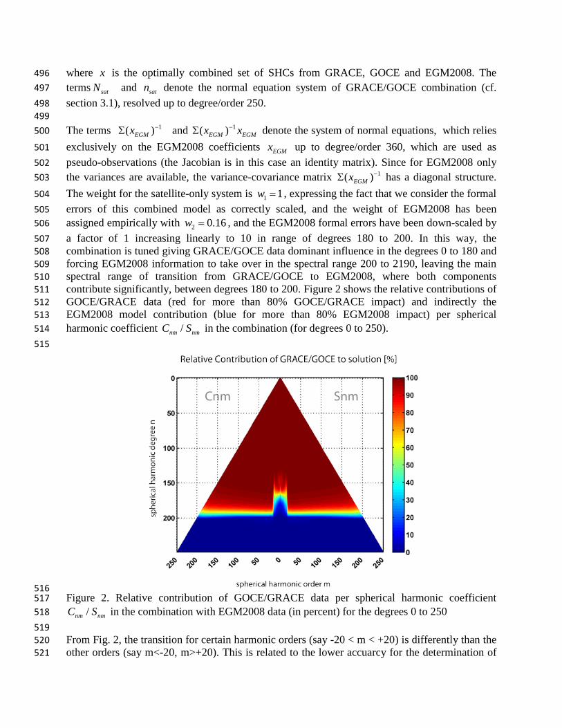
a factor of 1 increasing linearly to 10 in range of degrees 180 to 200. In this way, the 507 combination is tuned giving GRACE/GOCE data dominant influence in the degrees 0 to 180 and 508 forcing EGM2008 information to take over in the spectral range 200 to 2190, leaving the main 509 spectral range of transition from GRACE/GOCE to EGM2008, where both components 510 contribute significantly, between degrees 180 to 200. Figure 2 shows the relative contributions of 511 GOCE/GRACE data (red for more than 80% GOCE/GRACE impact) and indirectly the 512 EGM2008 model contribution (blue for more than 80% EGM2008 impact) per spherical 513 harmonic coefficient /nm nmC S in the combination (for degrees 0 to 250). 514

515

516 Figure 2. Relative contribution of GOCE/GRACE data per spherical harmonic coefficient 517

/nm nmC S in the combination with EGM2008 data (in percent) for the degrees 0 to 250 518

519 From Fig. 2, the transition for certain harmonic orders (say -20 < m < +20) is differently than the 520 other orders (say m<-20, m>+20). This is related to the lower accuarcy for the determination of 521

the near-zonal spherical harmonic coefficients using GOCE gradiometry (known as the polar gap 522 problem due to the GOCE satellite’s orbit inclination of 96.6 degrees). he lack of observations in 523 the polar regions worsens the accuracy in the determination of a certain group of spherical 524 harmonic coefficients, which is the near-zonal group (e.g., Sneeuw and Gelderen, 1997). 525 Consequently in the combined solution EGM2008 has a higher influence in for those coefficients 526 where GOCE shows a lower performance (and thus a higher standard deviation). 527 528 The outcome of this processing step is a combined GRACE/GOCE/EGM2008 coefficient data 529 set here denoted as GGE. Figure 3 shows the differences between gravity disturbances from 530 GGE and EGM2008, revealing significant discrepancies at the 10-20 mGal-level over Africa, 531 Asia and South America, while there is agreement in the mGal range over most parts of Europe, 532 Australia and North-America. The larger discrepancies are interpreted as improvements over 533 EGM2008 conferred by recent GRACE and GOCE data to GGMplus, see also Pail et al., [2011] 534 and Hirt et al., [2012]. 535 536

537 Figure 3. Gravity disturbance differences between the GRACE/GOCE/EGM2008 merger GGE 538 and EGM2008-only in the spectral band of degrees 2 to 250, units in mGal 539 540 3.3 Synthesis 541 542 The spherical-harmonic coefficients (SHCs) of the combined GGE model were used in the 543 spectral band of degrees 2 to 2190 to synthesize gravity field functionals at the Earth’s surface, 544 as represented through the 3D-coordinates (latitude, longitude, height). Accurate evaluation of 545 the SHCs requires taking into account the ellipsoidal height of the evaluation points which were 546 obtained from SRTM at 7.2 arc-second resolution. The zonal harmonics of the GRS80 normal 547 gravity field were subtracted from the GGE-model SHCs as described in Smith [1998]. The tide 548 system used in the synthesis is zero-tide, which is compatible with GRS80 [Moritz, 2000]. 549 550 Spherical harmonic synthesis of gravity field functionals at the Earth’s surface – known as 3D 551 synthesis – is computationally extraordinarily demanding, because efficient SHS operations 552

cannot be used [Holmes, 2003]. Therefore we used the gradient approach to higher order [Hirt, 553 2012] which offers an efficient yet accurate approximate solution for 3D synthesis at densely-554 spaced surface points, represented through the elevation model. We used a modification of the 555 harmonic_synth software [Holmes and Pavlis, 2008] to synthesize quasigeoid heights, gravity 556 disturbances, North-South and East-West deflections of the vertical at a reference height of 4 km 557 above the GRS80 reference ellipsoid at 1 arc-min resolution. For all four functionals radial 558 derivatives were computed up to 5th-order at the same reference height and resolution. These 559 were bicubically interpolated to 7.2 arc-second resolution and continued from the reference 560 height to the Earth’s surface with 5th-order Taylor series expansions (cf. generic formulations 561 provided in Hirt [2012]), yielding numerical estimates of gravity functionals at 3 billion surface 562 points in the spectral band of degrees 2 to 2190. 563 564 Using the gradient approach as described, the 3D synthesis of the four gravity field functionals 565 took about 6 weeks of computation time using an in-house Sun Ultra 45 workstation. By 566 comparison, 3D synthesis with conventional point-by-point evaluation methods [Holmes, 2003] 567 would have taken an estimated 60 years of computation time. This estimate is based on an 568 observed performance of 100 points/ minute using the same workstation and parameters. The 3D 569 synthesis as applied here is therefore one of the key innovations that made the construction of 570 GGMplus feasible within acceptable computation times. 571 572 We note that the gradient approach is an approximate technique for 3D-SHS, whereby 573 approximation errors decrease with increasing order of the Taylor series applied. From analysis 574 of the 0th to 5th-order contributions over 3 billion points, the contribution made by subsequent 575 orders (e.g., 0th and 1st, 1st and 2nd) differs by a factor of about 4 to 5 (see also Table 2). Given 576 maximum contributions of 2 mm, 0.6 mGal and 0.1 arc-sec for the 5th-order, maximum 577 approximation errors (due to truncation of the Taylor series after the 5th-order) will be generally 578 smaller than 0.6 mm, 0.2 mGal and 0.03 arc-sec anywhere in our working area. Hence, the 579 Taylor series as applied for GGMplus converge sufficiently, and approximation errors are 580 negligible for practical applications. 581 582 Table 2. RMS (root-mean-square) and maximum values of the 4th-order and 5th-order terms of 583 the Taylor expansions used for gravity field continuation to the Earth’s surface. Also given are 584 the estimated RMS and maximum approximation errors. Values reported for the functionals 585 quasigeoid, gravity disturbances and deflections of the vertical. 586 Functional Contribution of

4th –order term Contribution of 5th –order term

Estimated approximation error

RMS Max RMS Max RMS Max Quasigeoid [mm] 0.24 9.88 0.05 2.07 0.01 0.52 Gravity [mGal] 0.06 2.54 0.01 0.59 0.00 0.15 NS deflection of the vertical [arc-sec]

0.01 0.31 0.00 0.08 0.00 0.02

EW deflection of the vertical [arc-sec]

0.01 0.34 0.00 0.08 0.00 0.02

587 For quasigeoid heights, the C1B correction term [Rapp, 1997], see also [Hirt, 2012], was applied 588 to take into account the change in normal gravity with height. For gravity disturbances, the 589

ellipsoidal correction was applied [Claessens, 2006]. For the North-South deflection of the 590 vertical, corrections for the curvature of the plumbline and for the ellipsoidal effect were taken 591 into account as described in [Jekeli, 1999]. 592 593 594 3.4. Forward-modelling 595 596 Gravity forward-modelling based on high-resolution topography is a frequently-used technique 597 to derive information on the short-scale gravity field in approximation [Forsberg, 1984; Pavlis et 598 al., 2007; Hirt, 2012]. The short-scale (i.e., 10 km to ~250 m) gravity signals of the GGMplus 599 model are based on forward-modelling using the 7.5 arc-sec resolution (~250m) SRTM V4.1 600 topography [Jarvis et al., 2008] over land and the 30 arc-sec resolution SRTM30_PLUS V7.0 601 bathymetry [Becker et al., 2009] over sea. A small number of bad data areas (about 0.002% of 602 the total area covered by GGMplus as shown in Fig. 1) was identified and removed from both 603 data sets through simple hole-filling. 604 605 The forward-modelling approach applied here follows the description given in Hirt [2013]. In 606 brief, we converted the SRTM30_plus bathymetry to rock-equivalent depths before merging with 607 the 250m SRTM V4.1 topography. The merger was high-pass filtered by subtracting heights 608 from the RET2012 rock-equivalent topography model to degree and order 2160 (publicly 609 available from http://geodesy.curtin.edu.au/research/models/Earth2012/, 610 Earth2012.RET2012.SHCto2160.dat). 611 612 We applied brute-force numerical integration techniques [Forsberg, 1984] to convert the high-613 pass filtered topography (and rock-equivalent depths over sea) to topography-implied gravity, 614 geoid and vertical deflections. The forward-modelled gravity signals possess spectral energy at 615 spatial scales of ~10 km to ~250 m which augments GGE gravity information beyond 10 km 616 resolution. The numerical integration was accomplished with a variant of the TC software 617 [Forsberg, 1984] and an integration cap radius of 200 km around any of the ~3 billion 618 computation points, and the correction for Earth’s curvature applied, as described in Forsberg 619 [1984]. Given the oscillating nature of the high-pass filtered topography, the effect of remote 620 masses largely cancels out as pointed out by Forsberg and Tscherning [1981]. The integration 621 radius chosen is suitable for forward-modelling of high-frequency gravity effects [Hirt et al., 622 2010; Hirt, 2012]. 623 624 The forward-modelling exercise was partitioned into ~19,000 computationally ‘manageable’ 625 areas of 1 deg x 1 deg extension covering land areas everywhere on Earth between ± 60°-latitude 626 with SRTM data available. Each 1 deg x 1 deg tile is composed of 625,000 computation points at 627 7.2 arc-seconds resolution. We utilized the iVEC/Epic supercomputing facility 628 (http://www.ivec.org/) along with massive parallelization (simultaneous use of up to 1100 central 629 processing units (CPUs)) to accomplish the forward-modelling for the first time near-globally. 630 Based on non-parallelized standard computation techniques and a single CPU, the calculation of 631 topographic gravity effects had taken an estimated 20 years, which is why all previous efforts 632 were inevitably restricted to regional areas. 633 634

The topographic gravity effects calculations are based on the assumptions of constant mass-635 density (standard rock density 2670 kg/m3) and isostatically uncompensated topography, which 636 should well be justified given the spatial scales (less than 10 km) modelled here from 637 topographic information (e.g., Torge, [2001]; Watts, [2001]; Wieczorek, [2007]). Given that any 638 gravity field signals originating from mass-density variations [with respect to standard rock 639 density] are not represented by the topographic gravity, our GGMplus gravity maps cannot 640 provide geological information at scales less than 10 km. However, the same limitations apply to 641 EGM2008 at spatial scales less than ~27 km over many developing countries [Pavlis et al., 642 2012] and to any other gravity field model with topographic information used to increase the 643 resolution among observed gravity. 644 645 Due to the chosen constant mass-density - often used as standard mass-density for gravity 646 reductions in geophysics and geodesy - the chosen value should approximates well the 647 topographically-induced gravitational attraction over granite rock (2700 kg m-3), while the 648 approximation may introduce errors up to 7% over areas of volcanic rock (2900 kg m-3), and 649 about ~26 % where sediments prevail (2000 kg m-3). While inclusion of detailed mass-density 650 maps in the forward-modelling can reduce these errors, a detailed modelling of mass-density 651 variations was not attempted in this work because high-resolution density maps were not 652 available everywhere in our working area. 653 654 From comparisons with ground-truth data sets, a range of studies [e.g., Hirt et al., 2010; Hirt, 655 2012; Šprlák et al., 2012] demonstrate that short-scale topographic gravity effects are capable of 656 representing a significant portion (in some cases as high as 90 %) of real gravity field features 657 over rugged terrain, see also evaluation results in Section 5. 658 659 3.5 Calculation of normal gravity at the Earth’s surface 660 661 For the construction of gravity acceleration maps, normal gravity (i.e., the gravitational attraction 662 and centrifugal acceleration generated by an oblate equipotential ellipsoid of revolution) was 663 calculated at the Earth’s surface. We used the parameters of the GRS80 reference ellipsoid 664 [Moritz, 2000] along with the standard second-order Taylor expansion (Torge [2001], p 110, Eq. 665 4.63) to calculate normal gravity at the ellipsoidal heights of the Earth’s surface, as represented 666 through the SRTM topography at 7.2 arc-sec spatial resolution. Beside the gravitational 667 attraction and centrifugal acceleration of the GRS80 mass-ellipsoid, the resulting normal gravity 668 values also contain the effect of gravity attenuation with height (free-air effect), because we 669 evaluated at the Earth’s surface. 670 671 3.6 Combination of synthesis results, forward-modelling and normal gravity 672 673 All GGMplus gravity field functionals (quasigeoid heights, gravity disturbances, vertical 674 deflections) are the sum of 675

• Synthesized functionals from the GGE SHCs (providing the spatial scales of ~10000 km 676 down to ~10 km, Sect. 3.3) and 677

• Forward-modelled functionals from high-pass filtered topography/bathymetry data 678 (providing the spatial scales from ~10 km down to ~250 m, Sect. 3.4). 679

GGMplus gravity accelerations were obtained as the sum of GGMplus gravity disturbances and 680 normal gravity values (Sect 3.5). 681 682

4 Gravity estimation outside working area 683 684 Due to Earth’s flattening, obvious candidate locations for Earth’s maximum gravity acceleration 685 are expected near the poles, which is outside the ± 60°-SRTM latitude band. To include a likely 686 location for Earth’s maximum gravity acceleration in our work, we obtained gravity 687 accelerations globally at 5-arc-min resolution without short-scale topographic gravity estimates, 688 as follows: 689

1 We constructed a 5-arcmin grid of approximate ellipsoidal heights of the Earth’s surface 690 as the sum of elevations from the Earth2012 Topo/Air model (representing Earth’s 691 physical surface as lower interface of the atmosphere above mean sea level) and the 692 EGM2008 quasigeoid applied as a correction. 693

2 We applied the gradient approach for harmonic synthesis (Sect. 3.3) to fifth-order, 694 yielding gravity disturbances at the Earth’s surface in spectral band 2 to 2190 using the 695 GGE coefficients (Sect 3.1). 696

3 We calculated normal gravity at the ellipsoidal heights of the Earth’s surface as described 697 in Sect 3.5) and added the gravity disturbances, yielding gravity accelerations at 5 arc-698 min resolutions. 699

Steps 1 and 2 were applied to calculate a global 5 x 5 arc-min grid of quasigeoid heights which 700 was then used to locate where the quasigeoid is likely to be furthest below the ellipsoid. The 701 locations of the minimum and maximum gravity accelerations and quasigeoid heights are 702 reported in Tables S3 and S4. 703 704 Table 3. Extreme values of gravity accelerations estimated based on 5 arc-min resolution 705 Extreme value Latitude Longitude Value [mGal] Comment Minimum gravity acceleration

-9.88 -77.21 976790 GGMplus suggests a smaller value at a nearby location.

Maximum gravity acceleration

86.71 61.29 983366 Located offshore in the Arctic sea, not covered by GGMplus. Location and value reported in Table 1 in the main paper.

706 Table 4. Extreme values of quasigeoid heights estimated based on 5 arc-min resolution 707 Extreme value Latitude Longitude Value [m] Comment Minimum quasigeoid height

4.71 78.79 -106.59 Located offshore (Laccadive Sea, South of Sri Lanka), not covered by GGMplus. Location and value reported in Table 1 in the main paper.

Maximum quasigeoid height

-4.21 138.71 86.48 GGMplus suggests a larger value at another location.

708

5. Model evaluation 709 710 We have evaluated GGMplus gravity field functionals using (i) gravity accelerations from 711 terrestrial gravimetry, (ii) deflections of the vertical from geodetic-astronomical observations, 712 and (iii) observed quasigeoid heights from GPS ellipsoidal heights and geodetic levelling 713 (GPS/levelling). The data sets used are summarized in Table 5. Each set of observations is 714 compared against the three modelling variants 715 716

• satellite-only gravity (GRACE combined with 4th-GOCE release) to degree and order 200 717 (resolution of ~100 km) 718

• satellite gravity combined with EGM2008 (GGE), to degree 2190 (resolution of ~10 km) 719 • GGMplus (resolution of ~200 m) 720

721 The descriptive statistics of the differences “observation minus model” are reported in Tables 6 722 and 7 for gravity disturbances, in Table 8 for deflections of the vertical and in Table 9 for 723 quasigeoid heights. From the comparisons over North America, Europe and Australia – areas 724 with good ground gravity coverage – the accuracy of GGMplus is at the 3-5 mGal, 1 arc-sec and 725 5-7 cm level or somewhat better for gravity, deflections of the vertical and quasigeoid heights, 726 respectively. The RMS-improvements conferred by the short-scale gravity modelling (compare 727 GGMplus with GGE) range between ~20 to ~90 % for the radial (gravity) and horizontal field 728 components (deflections of the vertical), and is lower (non-significant to ~40% over Switzerland 729 as an example of a mountainous region) for quasigeoid heights. Fig. 4 exemplifies the good 730 agreement between observed gravity and GGMplus over Australia. The differences mostly 731 reflect the effect of local mass-density variations, and can be used for geophysical interpretation. 732 Fig. 4 also shows oscillations of 1-2 mGal amplitude and ~200 km full-wavelength which are 733 likely to reflect the error level of GOCE satellite observations used in GGMplus. 734 735 Over less well-surveyed areas, the differences increase to ~8 to ~23 mGal, as is indicated by the 736 few ground gravity observations available. Given that the forward-modelling of gravity effects at 737 spatial scales of ~10 km to 200 m is based on a homogeneous procedure everywhere between ± 738 60° geographic latitude, there is no reason to assume a reduced performance over Asia, Africa 739 and South America. The deterioration rather reflects the limited data availability for EGM2008 at 740 spatial scales of ~100 to 10 km. The accuracy of GGMplus gravity field functionals is therefore 741 largely dependent on the EGM2008 model commission errors, which can be as high as ~30-35 742 cm for quasigeoid heights, and ~4 arc-seconds for deflections of the vertical [Pavlis et al., 2012]. 743 We therefore expect the GGMplus accuracy to deteriorate by factor 3-5 from well-surveyed to 744 poorly-surveyed continents. 745 746 Table 5. Gravity field observations used for evaluation of GGMplus. 747 Observation type

Country/ Area # Stations Data source/provider

Gravity accelerations and disturbances from terrestrial

United States 1,277,637 University of Texas at el Paso http://research.utep.edu/default.aspx?tabid=37229 2012 release

Australia 1,625,018 Geoscience Australia

gravimetry http://www.geoscience.gov.au 2013 release

Switzerland 31,598 Swisstopo, Dr U Marti Central Africa 41,148 Bureau Gravimétrique International,

Dr S Bonvalot India/Himalayas 7,562 Bureau Gravimétrique International,

Dr S Bonvalot Northern South-America

12,150 Bureau Gravimétrique International, Dr S Bonvalot

Deflections of the vertical from geodetic-astronomical observations

United States 3,396 National Geodetic Survey, Drs D Smith and Y Wang

Australia 1,063 Geoscience Australia/ Dr W Featherstone (Curtin University)

Europe 1,056 ETZ Zurich, Dr B Bürki; Swisstopo, Dr U Marti; first author’s own observations

GPS/levelling/ quasigeoid heights

United States 18972 National Geodetic Survey, http://www.ngs.noaa.gov/NGSDataExplorer/

Germany 675 Bundesamt für Kartographie und Geodäsie, U Schirmer

Switzerland 193 Swisstopo, Dr U Marti 748 Table 6. Descriptive statistics of the differences observed gravity minus models, units in mGal 749

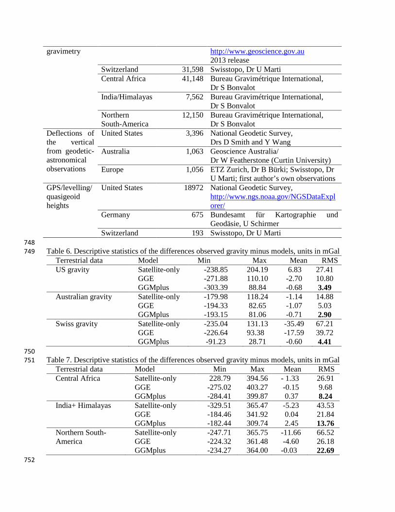
Terrestrial data Model Min Max Mean RMS US gravity Satellite-only -238.85 204.19 6.83 27.41 GGE -271.88 110.10 -2.70 10.80 GGMplus -303.39 88.84 -0.68 3.49 Australian gravity Satellite-only -179.98 118.24 -1.14 14.88 GGE -194.33 82.65 -1.07 5.03 GGMplus -193.15 81.06 -0.71 2.90 Swiss gravity Satellite-only -235.04 131.13 -35.49 67.21 GGE -226.64 93.38 -17.59 39.72 GGMplus -91.23 28.71 -0.60 4.41

750 Table 7. Descriptive statistics of the differences observed gravity minus models, units in mGal 751

Terrestrial data Model Min Max Mean RMS Central Africa Satellite-only 228.79 394.56 - 1.33 26.91 GGE -275.02 403.27 -0.15 9.68 GGMplus -284.41 399.87 0.37 8.24 India+ Himalayas Satellite-only -329.51 365.47 -5.23 43.53 GGE -184.46 341.92 0.04 21.84 GGMplus -182.44 309.74 2.45 13.76 Northern South- Satellite-only -247.71 365.75 -11.66 66.52 America GGE -224.32 361.48 -4.60 26.18 GGMplus -234.27 364.00 -0.03 22.69

752

753

754 Figure 4. Differences between observed gravity accelerations and GGMplus over Australia, units 755 in mGal. 756 757 Table 8. Descriptive statistics of the differences observed deflection of the vertical (DoV) minus 758 models, units in arc-seconds 759 Terrestrial data Model Min Max Mean RMS US North-South DoVs Satellite-only -19.59 22.62 0.20 3.27 GGE -12.55 21.29 0.09 1.11 GGMplus -12.58 20.97 -0.02 0.84 US East-West DoVs Satellite-only -22.66 23.41 0.29 3.78 GGE -13.57 12.38 0.10 1.14 GGMplus -6.19 9.90 0.12 0.78 Australian North-South DoVs Satellite-only -11.58 11.76 -0.14 2.21 GGE -5.00 3.44 -0.23 0.81 GGMplus -5.13 2.61 -0.19 0.66 Australian East-West DoVs Satellite-only -18.01 11.68 -0.14 2.63 GGE -4.87 3.60 -0.11 1.04 GGMplus -5.05 4.05 -0.13 0.97 Europe North-South DoVs Satellite-only -19.49 26.96 0.88 6.41 GGE -15.06 15.62 0.05 3.02 GGMplus -4.86 5.51 -0.05 1.06 Europe East-West DoVs Satellite-only -24.05 24.97 0.90 5.87 GGE -11.58 15.65 0.38 2.98 GGMplus -4.29 4.99 0.23 1.09

760 761 762 763

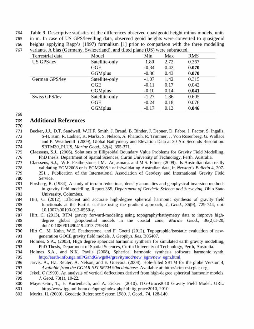
Table 9. Descriptive statistics of the differences observed quasigeoid height minus models, units 764 in m. In case of US GPS/levelling data, observed geoid heights were converted to quasigeoid 765 heights applying Rapp’s (1997) formalism [1] prior to comparison with the three modelling 766 variants. A bias (Germany, Switzerland), and tilted plane (US) were subtracted. 767 Terrestrial data Model Min Max RMS US GPS/lev Satellite-only 1.80 2.72 0.367 GGE -0.34 0.42 0.070 GGMplus -0.36 0.43 0.070 German GPS/lev Satellite-only -1.07 1.42 0.315 GGE -0.11 0.17 0.042 GGMplus -0.10 0.14 0.041 Swiss GPS/lev Satellite-only -1.27 1.86 0.605 GGE -0.24 0.18 0.076 GGMplus -0.17 0.13 0.046

768

Additional References 769 770 Becker, J.J., D.T. Sandwell, W.H.F. Smith, J. Braud, B. Binder, J. Depner, D. Fabre, J. Factor, S. Ingalls, 771

S-H. Kim, R. Ladner, K. Marks, S. Nelson, A. Pharaoh, R. Trimmer, J. Von Rosenberg, G. Wallace 772 and P. Weatherall (2009), Global Bathymetry and Elevation Data at 30 Arc Seconds Resolution: 773 SRTM30_PLUS, Marine Geod., 32(4), 355-371. 774

Claessens, S.J., (2006), Solutions to Ellipsoidal Boundary Value Problems for Gravity Field Modelling, 775 PhD thesis, Department of Spatial Sciences, Curtin University of Technology, Perth, Australia. 776

Claessens, S.J., W.E. Featherstone, I.M. Anjasmara, and M.S. Filmer (2009), Is Australian data really 777 validating EGM2008 or is EGM2008 just in/validating Australian data, in Newton’s Bulletin 4, 207-778 251 , Publication of the International Association of Geodesy and International Gravity Field 779 Service. 780

Forsberg, R. (1984), A study of terrain reductions, density anomalies and geophysical inversion methods 781 in gravity field modelling, Report 355, Department of Geodetic Science and Surveying, Ohio State 782 University, Columbus. 783

Hirt, C. (2012), Efficient and accurate high-degree spherical harmonic synthesis of gravity field 784 functionals at the Earth's surface using the gradient approach, J. Geod., 86(9), 729-744, doi: 785 10.1007/s00190-012-0550-y. 786

Hirt, C. (2013), RTM gravity forward-modeling using topography/bathymetry data to improve high-787 degree global geopotential models in the coastal zone, Marine Geod., 36(2):1-20, 788 doi:10.1080/01490419.2013.779334. 789

Hirt C., M. Kuhn, W.E. Featherstone, and F. Goettl (2012), Topographic/isostatic evaluation of new-790 generation GOCE gravity field models. J. Geophys. Res. B05407. 791

Holmes, S.A., (2003), High degree spherical harmonic synthesis for simulated earth gravity modelling, 792 PhD Thesis, Department of Spatial Sciences, Curtin University of Technology, Perth, Australia. 793

Holmes S.A., and N.K. Pavlis (2008), Spherical harmonic synthesis software harmonic_synth. 794 http://earth-info.nga.mil/GandG/wgs84/gravitymod/new_egm/new_egm.html. 795

Jarvis, A., H.I. Reuter, A. Nelson, and E. Guevara. (2008). Hole-filled SRTM for the globe Version 4, 796 Available from the CGIAR-SXI SRTM 90m database. Available at: http://srtm.csi.cgiar.org. 797

Jekeli C (1999), An analysis of vertical deflections derived from high-degree spherical harmonic models. 798 J. Geod. 73(1), 10-22. 799

Mayer-Gürr, T., E. Kurtenbach, and A. Eicker (2010), ITG-Grace2010 Gravity Field Model. URL: 800 http://www.igg.uni-bonn.de/apmg/index.php?id=itg-grace2010, 2010. 801

Moritz, H. (2000), Geodetic Reference System 1980. J. Geod., 74, 128-140. 802

Pail R., T. Fecher, M. Murböck M. Rexer, M. Stetter, T. Gruber, and C. Stummer, (2013), Impact of 803 GOCE Level 1b data reprocessing on GOCE-only and combined gravity field models. Stud. 804 Geophy. Geod. 57, 155-173. 805

Pavlis, N.K., J.K. Factor, and S.A. Holmes (2007), Terrain-related gravimetric quantities computed for 806 the next EGM, in Proceedings of the 1st International Symposium of the International Gravity Field 807 Service 318-323, Harita Dergersi, Istanbul. 808

Pavlis N.K., S.A. Holmes, S.C. Kenyon, and J.K. Factor (2012), The development and evaluation of the 809 Earth Gravitational Model 2008 (EGM2008), J. Geophys. Res., 117, B04406, 810 doi:10.1029/2011JB008916. 811

Rapp R.H (1997), Use of potential coefficient models for geoid undulation determinations using a 812 spherical harmonic representation of the height anomaly/geoid undulation difference, J. Geod. 71(5), 813 282-289. 814

Smith, D.A. (1998), There is no such thing as "The" EGM96 geoid: Subtle points on the use of a global 815 geopotential model, in International Geoid Service Bulletin 8, 17-28, International Geoid Service, 816 Milan, Italy. 817

Sneeuw N., van Gelderen, M. (1997), The polar gap. In: Geodetic boundary value problems in view of the 818 one centimeter geoid. Lecture notes in Earth Sciences, 65, 559–568, Springer, Berlin, 819 doi:10.1007/BFb0011699 820

Šprlák, M., C. Gerlach, and B.R. Pettersen, (2012), Validation of GOCE global gravity field models using 821 terrestrial gravity data in Norway. J. Geod. Sci. 2, 134-143. 822

Stummer C., T. Fecher, and R. Pail (2013), Alternative method for angular rate determination within the 823 GOCE gradiometer processing. J. Geod. 85, 585-596 (2011). 824

Torge, W. (2001), Geodesy, 3rd Edition., De Gruyter, Berlin, New York. 825 Watts, A.B. (2001), Isostasy and Flexure of the Lithosphere. Cambridge University Press. 826 Wieczorek M.A. (2007), Gravity and topography of the terrestrial planets, in Treatise on Geophysics 10, 827

165, Elsevier-Pergamon, Oxford. 828 829