Contents I

MEDICAL RADIOLOGYRadiation Oncology

Editors:L. W. Brady, Philadelphia

H.-P. Heilmann, HamburgM. Molls, Munich

Contents III

W. Schlegel · T. Bortfeld · A.- L. Grosu (Eds.)

New Technologies in Radiation Oncology

With Contributions by

J. R. Adler · N. Agazaryan · D. Baltas · Y. Belkacémi · R. Bendl · T. Bortfeld · L. G. BouchetG. T. Y. Chen · K. Eilertsen · M. Fippel · K. H. Grosser · A.-L. Grosu · P. Häring J.-M. Hannoun-Lévi · G. H. Hartmann · K. K. Herfarth · J. Hesser · R. HindererG. D. Hugo · O. Jäkel · M. Kachelriess · C. P. Karger · M. L. Kessler · C. KirisitsP. Kneschaurek · S. Kriminski · E. Lartigau · S.-L. Meeks · E. Minar · M. Molls · S. MuticS. Nill · U. Oelfke · D. R. Olsen · N. P. Orton · H. Paganetti · A. Pirzkall · R. PötterB. Pokrajac · A. Pommert · B. Rhein · E. Rietzel · M. A. Ritter · M. Roberson · G. SakasL. R. Schad · W. Schlegel · C. Sholz · A. Schweikard · T. D. Solberg · L. SpragueD. Stsepankou · S.E. Tenn · C. Thieke · W. A. Tomé · N. M. Wink · D. Yan · M. Zaider N. Zamboglou

Foreword by

L. W. Brady, H.-P. Heilmann and M. Molls

With 299 Figures in 416 Separate Illustrations, 246 in Color and 39 Tables

123

IV Contents

Wolfgang Schlegel, PhDProfessor, Abteilung Medizinische Physik in der Strahlentherapie Deutsches KrebsforschungszentrumIm Neuenheimer Feld 28069120 HeidelbergGermany

Thomas Bortfeld, PhDProfessor, Department of Radiation OncologyMassachusetts General Hospital 30, Fruit StreetBoston, MA 02114 USA

Anca-Ligia Grosu, MDPrivatdozent, Department of Radiation OncologyKlinikum rechts der Isar Technical University Munich Ismaningerstrasse 2281675 MünchenGermany

Medical Radiology · Diagnostic Imaging and Radiation OncologySeries Editors: A. L. Baert · L. W. Brady · H.-P. Heilmann · M. Molls · K. Sartor

Continuation of Handbuch der medizinischen Radiologie Encyclopedia of Medical Radiology

Library of Congress Control Number: 2004116561

ISBN 3-540-00321-5 Springer Berlin Heidelberg New YorkISBN 978-3-540-00321-2 Springer Berlin Heidelberg New York

This work is subject to copyright. All rights are reserved, whether the whole or part of the material is concerned, specifi -cally the rights of translation, reprinting, reuse of illustrations, recitations, broadcasting, reproduction on microfi lm or in any other way, and storage in data banks. Duplication of this publication or parts thereof is permitted only under the provisions of the German Copyright Law of September 9, 1965, in its current version, and permission for use must always be obtained from Springer-Verlag. Violations are liable for prosecution under the German Copyright Law.

Springer is part of Springer Science+Business Media

http//www.springeronline.com© Springer-Verlag Berlin Heidelberg 2006Printed in Germany

The use of general descriptive names, trademarks, etc. in this publication does not imply, even in the absence of a specifi c statement, that such names are exempt from the relevant protective laws and regulations and therefore free for general use.

Product liability: The publishers cannot guarantee the accuracy of any information about dosage and application contained in this book. In every case the user must check such information by consulting the relevant literature.

Medical Editor: Dr. Ute Heilmann, HeidelbergDesk Editor: Ursula N. Davis, HeidelbergProduction Editor: Kurt Teichmann, MauerCover-Design and Typesetting: Verlagsservice Teichmann, Mauer

Printed on acid-free paper – 21/3151xq – 5 4 3 2 1 0

Contents V

Radiation oncology is one of the most important treatment facilities in the management of malignant tumors. Although this specialty is in the first line a physician’s task, a variety of technical equipment and technical know-how is necessary to treat patients in the most effective way possible today.

The book by Schlegel et al., “New Technologies in Radiation Oncology,” provides an overview of recent advances in radiation oncology, many of which have originated from physics and engineering sciences. 3D treatment planning, conformal radiotherapy, with consideration of both external radiotherapy and brachytherapy, stereotactic radiotherapy, intensity-modulated radiation therapy, image-guided and adaptive radiotherapy, and radiotherapy with charged particles are described meticulously . Because radiotherapy is a doctor’s task, clinically orientated chapters explore the use of therapeutic radiology in different oncologic situations. A chapter on quality assurance concludes this timely pub-lication.

The book will be very helpful for doctors in treating patients as well as for physicists and other individuals interested in oncology.

Philadelphia Luther W. BradyHamburg Hans-Peter HeilmannMunich Michael Molls

Foreword

Contents VII

Preface

In the 1960s radiation therapy was considered an empirical, clinical discipline with a relatively low probability of success. This situation has changed considerably during the past 40 years.

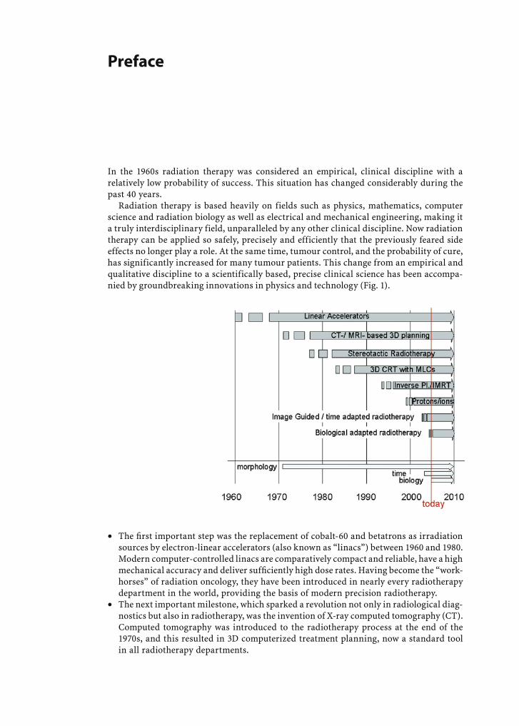
Radiation therapy is based heavily on fields such as physics, mathematics, computer science and radiation biology as well as electrical and mechanical engineering, making it a truly interdisciplinary field, unparalleled by any other clinical discipline. Now radiation therapy can be applied so safely, precisely and efficiently that the previously feared side effects no longer play a role. At the same time, tumour control, and the probability of cure, has significantly increased for many tumour patients. This change from an empirical and qualitative discipline to a scientifically based, precise clinical science has been accompa-nied by groundbreaking innovations in physics and technology (Fig. 1).

∑ The fi rst important step was the replacement of cobalt-60 and betatrons as irradiation sources by electron-linear accelerators (also known as “linacs”) between 1960 and 1980. Modern computer-controlled linacs are comparatively compact and reliable, have a high mechanical accuracy and deliver suffi ciently high dose rates. Having become the “work-horses” of radiation oncology, they have been introduced in nearly every radiotherapy department in the world, providing the basis of modern precision radiotherapy.

∑ The next important milestone, which sparked a revolution not only in radiological diag-nostics but also in radiotherapy, was the invention of X-ray computed tomography (CT). Computed tomography was introduced to the radiotherapy process at the end of the 1970s, and this resulted in 3D computerized treatment planning, now a standard tool in all radiotherapy departments.

VIII Contents

∑ The CT-based treatment planning was later supplemented with medical resonance imaging (MRI). By combining CT and MRI, and using registered images for radio-therapy planning, it is now possible to assess tumour morphology more precisely, and thus achieve improved defi nition of planning target volumes (PTV), improving both percutaneous radiotherapy and brachytherapy.

∑ The computer revolution, characterized by the development of small, powerful and inexpensive desktop computers, had tremendous impact on radiation therapy. With new tools from 3D computer graphics, implemented in parallel with 3D treatment plan-ning, it was possible to establish “virtual radiotherapy planning”, a method to plan and simulate 3D irradiation techniques. New 3D dose calculation algorithms (e.g. “pencil-beam algorithms”) made it possible to precalculate the 3D dose distributions with suf-fi cient accuracy and with acceptable computing times.

∑ With the aforementioned advent of 3D imaging, 3D virtual therapy simulation and 3D dose calculation, the preconditions for introducing an individualized, effective local radiation treatment of tumours were fulfi lled. What was still missing was the possibil-ity to transfer the computer plans to the patient with high accuracy. This gap was fi lled by the introduction of stereotaxy into radiotherapy in the early 1980s. Prior to this development, stereotaxy was used in neurosurgery as a tool to precalculate target points in the brain and to precisely guide probes to these target points within the tumour in order to take biopsies or implant radioactive seeds. The transfer of this technique to radiotherapy resulted in signifi cantly enhanced accuracy in patient positioning and adjustment of radiation beams. Stereotactic treatment techniques were fi rst developed for single-dose irradiations (called “radiosurgery”), then for fractionated treatments in the brain and the head and neck region (“stereotactic radiotherapy”). Later, it became possible to transfer stereotactic positioning to extracranial tumour locations (“extra-cranial stereotactic radiotherapy”) as well. This opened up the possibility for high-pre-cision treatments of tumours in nearly all organs and locations.

∑ The next important step which revolutionized radiotherapy came again from the fi eld of engineering. The development of computerized multi-leaf collimators (MLCs) in the middle of the 1980s ensured the clinical breakthrough of 3D conformal radiotherapy. With the advent of MLCs, the time-consuming fabrication of irregularly shaped beams with cerrobend blocks could be abandoned. Conformal treatments became less expen-sive and considerably faster, and were applied with increasing frequency. The combi-nation of 3D treatment planning and 3D conformal beam delivery resulted in safe and effi cient treatment techniques, which allowed therapists to escalate tumour doses while at the same time lowering the dose in organs at risk and normal tissues.

∑ By the mid 1990s, 3D conformal radiotherapy was supplemented by a new treatment technique, which is currently becoming a standard tool in modern clinics: intensity-modulated radiotherapy (IMRT) using MLC-beam delivery or tomotherapy, in combi-nation with inverse treatment planning. In IMRT the combination of hardware and soft-ware techniques solves the problem of irradiating complex target volumes with concave parts in the close vicinity of critical structures, a problem with which radio-oncologists have had to struggle from the very beginning of radiotherapy. In many modern clinics around the world, IMRT is successfully applied, e.g. in the head and neck and in pros-tate cancer. It has the potential to improve results in many other cancer treatments as well.

∑ The IMRT with photon beams can achieve a level of conformity of the dose distribution within the target volume which can, from a physical point of view, not be improved further; however, the absolute dose which can be delivered to the target volume is still limited by the unavoidable irradiation exposure of the surrounding normal tissue. A further improvement of this situation is possible by using particle radiation. Compared with photon beams, the interaction of particle beams (like protons or heavier charged particles) with tissue is completely different. For a single beam, the dose delivered to

Contents IX

the patient has a maximum shortly before the end of the range of the particles. This is much more favourable compared with photons, where the dose maximum is located just 2–3 cm below the surface of the patient’s body. By selecting an appropriate energy for the particle beams and by scanning particle pencil beams over the whole target volume, highly conformal dose distributions can be reached, with a very steep dose fall-off to surrounding tissue, and a much lower “dose bath” to the whole irradiated normal tissue volume. Furthermore, from the use of heavier charged particles, such as carbon-12 or oxygen-16, an increase in RBE can be observed shortly before the end of the range of the particles. It is expected that this radiobiological advantage over photons and pro-tons will result in a further improvement in local control, especially for radioresistant tumours. However, particle therapy, both with protons and heavier charged particles, is still in the early stages of clinical application and evaluation on a broad scale. Ongoing and future clinical trials must demonstrate the benefi t of these promising, but costly, particle-beam treatments.

At the beginning of the new millennium, the field of adaptive radiotherapy evolved from radio-oncology:∑ After 3D CT and MRI enabled a much better understanding of tumour morphology,

and thus spatial delineation of target volumes, the time has arrived where the temporal alterations of the target volume can also be assessed and taken into account. Image-guided and time-adapted radiotherapy (IGRT and ART) are characterized by the inte-gration of 2D and 3D imaging modalities into the radiotherapy work fl ow. The vision is to detect deformations and motion between fractions (inter-fractional IGRT) and during irradiation (intra-fractional IGRT), and to correct for these changes either by gating or tracking of the irradiation beam. Several companies in medical engineering are currently addressing this technical challenge, with the goal of implementing IGRT and ART in radiotherapy as a fast, safe and effi cient treatment technique.

∑ Another innovation which is currently on the horizon is biological adaptive radiother-apy. The old hypothesis that the tumour consists of homogeneous tissue, and therefore a homogeneous dose distribution is suffi cient, can no longer be sustained. We now know that a tumour may consist of different subvolumes with varying radiobiological proper-ties. We are trying to characterize these properties more appropriately by functional and molecular imaging using new tracers in PET and SPECT imaging and by functional MRI (fMRI) and MR spectroscopy, for example. We now have to develop concepts to include and integrate this information into radiotherapy planning and beam delivery, fi rstly by complementing the morphological gross tumour volume (GTV) by a biologi-cal target volume (BTV) consisting of subvolumes of varying radioresistance, and sec-ondly by delivering appropriate inhomogeneous dose distributions with the new tools of photon- and particle-IMRT techniques (“dose painting”). Furthermore, biological imaging can give additional information concerning tumour extension and tumour response to radiotherapy or radiochemotherapy.

Currently, we have reached a point where, besides the 3D tumour morphology, time variations and biological variability within the tumour can also be taken into account. The repertoire of radiation oncology has thus been expanded tremendously. Tools and methods applied to radiotherapy are increasing in number and complexity. The speed of these devel-opments is sometimes breathtaking, as radiation oncologists are faced more and more with the problem of following and understanding these modern innovations in their profession, and putting the new developments into practice. This book gives an introduction into the aforementioned areas. The authors of the various chapters are specialists from the involved disciplines, either working in research and development or in integrating and using the new methods in clinical application. The authors endeavoured to explain the very often complicated and complex subject matter in an understandable manner. Naturally, such a

X Contents

collection of contributions from a heterogeneous board of authors cannot completely cover the whole field of innovations. Some overlap, and variations in the depth of descriptions and explanations were unavoidable. We hope that the book will be particularly helpful for physicians and medical physicists who are working in radiation oncology or just entering the field, and who are trying to achieve an overview and a better understanding of the new technologies in radiation oncology.

The motivation to compile this book can be traced back to the editors of the book series Medical Radiology/Radiation Oncology, by Michael Molls, Munich, Luther Brady, Philadel-phia, and Hans-Peter Heilmann, Hamburg. We thank them for continuous encouragement and for not losing the belief that the work will eventually be finished. We extend thanks to Alan Bellinger, Ursula Davis, Karin Teichmann and Kurt Teichmann, who did such an excellent job in preparing the book. Most of all, thanks to all the authors, who wrote their chapters according to our suggestions, and a very special thanks to those who did this work within the short period of time before the deadline.

Heidelberg Wolfgang SchlegelBoston Thomas BortfeldMunich Anca-Ligia Grosu

Contents XI

1 New Technologies in 3D Conformal Radiation Therapy: Introduction and Overview

W. Schlegel . . . . . . . . . . . . . . . . . . . . . . . . . . . . . . . . . . . . . . . . . . . . . . . . . . . . . . . . . . . . . 1

Basics of 3D Imaging . . . . . . . . . . . . . . . . . . . . . . . . . . . . . . . . . . . . . . . . . . . . . . . . . . . . . . . 7

2 3D Reconstruction J. Hesser and D. Stsepankou. . . . . . . . . . . . . . . . . . . . . . . . . . . . . . . . . . . . . . . . . . . . . 9

3 Processing and Segmentation of 3D Images G. Sakas and A. Pommert . . . . . . . . . . . . . . . . . . . . . . . . . . . . . . . . . . . . . . . . . . . . . . . 17

4 3D Visualization G. Sakas and A. Pommert . . . . . . . . . . . . . . . . . . . . . . . . . . . . . . . . . . . . . . . . . . . . . . . 24

5 Image Registration and Data Fusion for Radiotherapy Treatment Planning M. L. Kessler and M. Roberson . . . . . . . . . . . . . . . . . . . . . . . . . . . . . . . . . . . . . . . . . . 41

6 Data Formats, Networking, Archiving, and Telemedicine K. Eilertsen and D. R. Olsen . . . . . . . . . . . . . . . . . . . . . . . . . . . . . . . . . . . . . . . . . . . . 53

3D Imaging for Radiotherapy . . . . . . . . . . . . . . . . . . . . . . . . . . . . . . . . . . . . . . . . . . . . . . . 65

7 Clinical X-Ray Computed Tomography M. Kachelriess . . . . . . . . . . . . . . . . . . . . . . . . . . . . . . . . . . . . . . . . . . . . . . . . . . . . . . . . 67

8 4D Imaging and Treatment Planning E. Rietzel and G. T. Y. Chen . . . . . . . . . . . . . . . . . . . . . . . . . . . . . . . . . . . . . . . . . . . . . 81

9 Magnetic Resonance Imaging for Radiotherapy Planning L. R. Schad. . . . . . . . . . . . . . . . . . . . . . . . . . . . . . . . . . . . . . . . . . . . . . . . . . . . . . . . . . . . . 99

10 Potential of Magnetic Resonance Spectroscopy for Radiotherapy Planning A. Pirzkall . . . . . . . . . . . . . . . . . . . . . . . . . . . . . . . . . . . . . . . . . . . . . . . . . . . . . . . . . . . . 113

11 PET and PET/CT for Radiotherapy Planning S. Mutic . . . . . . . . . . . . . . . . . . . . . . . . . . . . . . . . . . . . . . . . . . . . . . . . . . . . . . . . . . . . . . . 131

12 Patient Positioning in Radiotherapy Using Optical Guided 3D-Ultrasound Techniques

W. A. Tomé, S. L. Meeks, N. P. Orton, L. G. Bouchet, and M. A. Ritter . . . . . . 151

Contents

XII Contents

3D Treatment Planning for Conformal Radiotherapy . . . . . . . . . . . . . . . . . . . . . . . . . . 165

13 Definition of Target Volume and Organs at Risk. Biological Target Volume

A.-L. Grosu, L. D. Sprague, and M. Molls . . . . . . . . . . . . . . . . . . . . . . . . . . . . . . . . 167

14 Virtual Therapy Simulation R. Bendl . . . . . . . . . . . . . . . . . . . . . . . . . . . . . . . . . . . . . . . . . . . . . . . . . . . . . . . . . . . . . . . 179

15 Dose Calculation Algorithms U. Oelfke and C. Scholz . . . . . . . . . . . . . . . . . . . . . . . . . . . . . . . . . . . . . . . . . . . . . . . . 187

16 Monte Carlo Dose Calculation for Treatment Planning Matthias Fippel . . . . . . . . . . . . . . . . . . . . . . . . . . . . . . . . . . . . . . . . . . . . . . . . . . . . . . . 197

17 Optimization of Treatment Plans, Inverse Planning T. Bortfeld and C. Thieke. . . . . . . . . . . . . . . . . . . . . . . . . . . . . . . . . . . . . . . . . . . . . . . 207

18 Biological Models in Treatment Planning C. P. Karger. . . . . . . . . . . . . . . . . . . . . . . . . . . . . . . . . . . . . . . . . . . . . . . . . . . . . . . . . . . . 221

19 2D and 3D Planning in Brachytherapy D. Baltas and N. Zamboglou . . . . . . . . . . . . . . . . . . . . . . . . . . . . . . . . . . . . . . . . . . . . 237

New Treatment Techniques . . . . . . . . . . . . . . . . . . . . . . . . . . . . . . . . . . . . . . . . . . . . . . . . . 255

20 Beam Delivery in 3D Conformal Radiotherapy Using Multi-Leaf Collimators W. Schlegel, K. H. Grosser , P. Häring, and B. Rhein . . . . . . . . . . . . . . . . . . . . . 257

21 Stereotactic Radiotherapy/Radiosurgery A.-L. Grosu, P. Kneschaurek, and W. SchlegeL. . . . . . . . . . . . . . . . . . . . . . . . . . . . 267

22 Extracranial Stereotactic Radiation Therapy K. K. Herfarth . . . . . . . . . . . . . . . . . . . . . . . . . . . . . . . . . . . . . . . . . . . . . . . . . . . . . . . . . 277

23 X-MRT S. Nill, R. Hinderer and U. Oelfke . . . . . . . . . . . . . . . . . . . . . . . . . . . . . . . . . . . . . . 289

24 Control of Breathing Motion: Techniques and Models (Gated Radiotherapy)

T. D. Solberg, N. M. Wink, S. E. Tenn, S. Kriminski, G. D. Hugo, and N. Agazaryan . . . . . . . . . . . . . . . . . . . . . . . . . . . . . . . . . . . . . . . . . . . . . . . . . . . . . . 299

25 Image-Guided/Adaptive Radiotherapy D. Yan . . . . . . . . . . . . . . . . . . . . . . . . . . . . . . . . . . . . . . . . . . . . . . . . . . . . . . . . . . . . . . . . . 321

26 Predictive Compensation of Breathing Motion in Lung Cancer Radiosurgery

A. Schweikhard and J. R. Adler . . . . . . . . . . . . . . . . . . . . . . . . . . . . . . . . . . . . . . . . . 337

27 Proton Therapy H. Paganetti and T. Bortfeld . . . . . . . . . . . . . . . . . . . . . . . . . . . . . . . . . . . . . . . . . . . 345

Contents XIII

28 Heavy Ion Radiotherapy O. Jäkel. . . . . . . . . . . . . . . . . . . . . . . . . . . . . . . . . . . . . . . . . . . . . . . . . . . . . . . . . . . . . . . . 365

29 Permanent-Implant Brachytherapy in Prostate Cancer M. Zaider . . . . . . . . . . . . . . . . . . . . . . . . . . . . . . . . . . . . . . . . . . . . . . . . . . . . . . . . . . . . . . 379

30 Vascular Brachytherapy B. Pokrajac, E. Minar, C. Kirisits, and R. Pötter . . . . . . . . . . . . . . . . . . . . . . . . . 389

31 Partial Breast Brachytherapy After Conservative Surgery for Early Breast Cancer: Techniques and Results

Y. Belkacémi, J.-M. Hannoun-Lévi, and E. Lartigau. . . . . . . . . . . . . . . . . . . . . . . 397

Verification and QA . . . . . . . . . . . . . . . . . . . . . . . . . . . . . . . . . . . . . . . . . . . . . . . . . . . . . . . . 409

32 3D Quality Assurance (QA) Systems B. Rhein and P. Häring . . . . . . . . . . . . . . . . . . . . . . . . . . . . . . . . . . . . . . . . . . . . . . . . . 411

33 Quality Management in Radiotherapy G. Hartmann . . . . . . . . . . . . . . . . . . . . . . . . . . . . . . . . . . . . . . . . . . . . . . . . . . . . . . . . . . 425

Subject Index . . . . . . . . . . . . . . . . . . . . . . . . . . . . . . . . . . . . . . . . . . . . . . . . . . . . . . . . . . . . . . . 449

List of Contributors . . . . . . . . . . . . . . . . . . . . . . . . . . . . . . . . . . . . . . . . . . . . . . . . . . . . . . . . . 457

New Technologies in 3D Conformal Radiation Therapy: Introduction and Overview 1

1 New Technologies in 3D Conformal Radiation Therapy: Introduction and Overview

Wolfgang Schlegel

W. Schlegel, PhDProfessor, Abteilung Medizinische Physik in der Strahlen-therapie, Deutsches Krebsforschungszentrum, Im Neuen-heimer Feld 280, 69120 Heidelberg, Germany

1.1 Clinical Demand for New Technologies in Radiotherapy

Radiotherapy is, after surgery, the most successfully and most frequently used treatment modality for cancer. It is applied in more than 50% of all cancer patients.

Radiotherapy aims to deliver a radiation dose to the tumor which is high enough to kill all tumor cells. That is from the physical and technical point of view a diffi cult task, because malignant tumors often are located close to radiosensitive organs such as the eyes, optic nerves and brain stem, spinal cord, bow-els, or lung tissue. These so-called organs at risk must not be damaged during radiotherapy. The situation is even more complicated when the tumor itself is radi-oresistant and very high doses are needed to reach a therapeutic effect.

At the time of being diagnosed, about 60% of all tumor patients are suffering from a malignant local-ized tumor which has not yet disseminated, i.e., no metastatic disease has yet occurred; thus, these pa-tients can be considered to be potentially curable. Nevertheless, about one-third of these patients (18% of all cancer patients) cannot be cured, because ther-apy fails to stop tumor growth.

This is the point where new technologies in radia-tion oncology, especially in 3D conformal radiother-apy, come into play: it is expected that they will en-hance local tumor control. In conformal radiotherapy, the dose distribution in tissue is shaped in such a way that the high-dose region is located in the target vol-ume, with a maximal therapeutic effect throughout the whole volume. In the neighboring healthy tissue, the radiation dose has to be kept under the limit for radiation damage. This means a steep dose falloff has to be reached between the target volume and the sur-roundings; thus, in radiotherapy there is a rule stat-ing that with a decrease of dose to healthy tissue, the dose delivered to the target volume can be increased; moreover, an increase in dose will also result in bet-ter tumor control (tumor control probability, TCP), whereas a decrease in dose to healthy tissue will be connected with a decrease in side effects (normal tissue complication probability, NTCP). Increase in tumor control and a simultaneous decrease in side effects means a higher probability of patient cure.

In the past two decades, new technologies in ra-diation oncology have initiated a signifi cant increase in the quality of conformal treatment techniques. The development of new technologies for conformal radiation therapy is the answer to the wishes and guidelines of the radiation oncologists. The ques-tion of whether clinical improvements are driven by new technical developments, or vice versa, should be answered in the following way: the development of new technologies should be motivated by clinical constraints.

In this regard the physicists, engineers, computer scientists, and technicians are service providers to the radiologists and radiotherapists, and in this con-

CONTENTS

1.1 Clinical Demand for New Technologies in Radiotherapy 11.2 Basic Principles of Conformal Radiotherapy 21.3 Clinical Workfl ow in Conformal Radiotherapy 21.3.1 Patient Immobilization 31.3.2 Imaging and Tumor Localization 31.3.3 Treatment Planning 31.3.3.1 Defi ning Target Volumes and Organs at Risk 31.3.3.2 Defi nition of the Treatment Technique 41.3.3.3 Dose Calculation 41.3.3.4 Evaluation of the 3D Dose Distribution 41.4 Patient Positioning 41.5 Treatment 51.5.1 Photons 51.5.2 Charged-Particle Therapy 51.5.3 Brachytherapy 51.6 Quality Management in Radiotherapy 5 References 6

2 W. Schlegel

text new technologies in conformal radiation therapy are technical answers to a clinical challenge.

An improvement in one fi eld automatically en-tails the necessity of an improvement in other fi elds. Conformal radiation therapy combines, in the best case, the advantages of all new developments.

1.2 Basic Principles of Conformal Radiotherapy

The basic idea of conformal radiation therapy is easy to understand and it is close to being trivial (Fig. 1.1). The problem is that depth dose of a homogeneous photon fi eld is described by an exponentially de-creasing function of depth. Dose deposition is nor-mally higher close to the surface than at the depth of the tumor.

To improve this situation normally more than one beam is used. Within the overlapping region of the beams a higher dose is deposited. If the apertures of the beams are tailored (three dimensionally) to the shape of the planning target volume (PTV) masking the organs at risk (OAR), then the overlapping region should fi t the PTV. In the case of an OAR close to the PTV, this is not true for such a simple beam confi gu-ration such as the one shown in Fig. 1.1. In such cases one needs a more complex beam confi guration to achieve an acceptable dose distribution; however, the general thesis is that, using enough beams, it should be possible to a certain extent to fi t a homogeneous

dose distribution to the PTV while sparing the OARs. One hopes that the conformity of dose distributions can be increased using individually tailored beams compared with, for example, a beam arrangement using simple rectangular-shaped beams, and for the majority of cases this is true. Nevertheless, there are cases, especially with concave-shaped target volumes and moving targets, where conventional conformal treatment planning and delivery techniques fail. It is hoped that these problems will be solved using inten-sity-modulated radiotherapy (IMRT; see Chap. 23) and adaptive radiotherapy (ART; see Chaps. 24–26), respectively.

1.3 Clinical Workfl ow in Conformal Radiotherapy

The physical and technical basis of the radiation therapy covers different aspects of all links in the “chain of radiotherapy” (Fig. 1.2) procedure. All parts of the “chain of radiation therapy” are discussed in other chapters separately and in great detail, and an overview on the structure of this book within this context is given in Table 1.1.

Table 1.1 Structure of the book with respect to the chain of radiotherapy

Part of the radiotherapy chain Described in chapter

Patient immobilization 21, 22Imaging and information processing 2–6Tumor localization 7–11Treatment planning 13, 14Patient positioning 12, 21, 22, 26Treatment 20–28Quality assurance and verifi cation 32, 33

Target volume

Organ at risk

Dose

Fig. 1.1. Basic idea of conformal radiotherapy

Fig. 1.2. Chain of radiotherapy. (From Schlegel and Mahr 2001)

New Technologies in 3D Conformal Radiation Therapy: Introduction and Overview 3

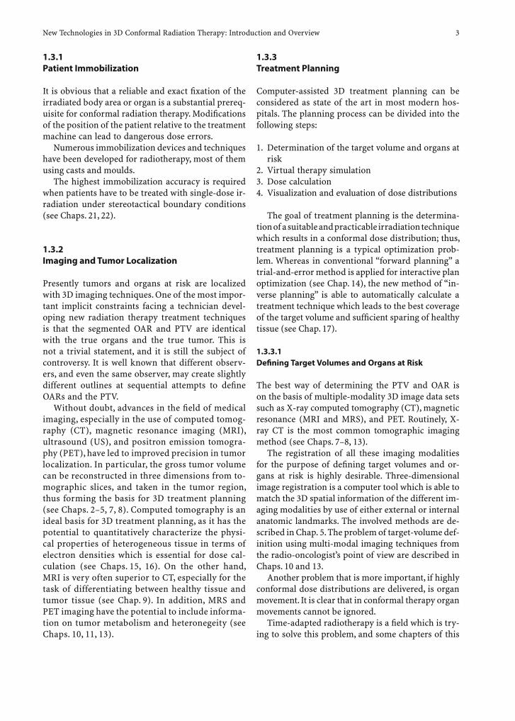
1.3.1 Patient Immobilization

It is obvious that a reliable and exact fi xation of the irradiated body area or organ is a substantial prereq-uisite for conformal radiation therapy. Modifi cations of the position of the patient relative to the treatment machine can lead to dangerous dose errors.

Numerous immobilization devices and techniques have been developed for radiotherapy, most of them using casts and moulds.

The highest immobilization accuracy is required when patients have to be treated with single-dose ir-radiation under stereotactical boundary conditions (see Chaps. 21, 22).

1.3.2 Imaging and Tumor Localization

Presently tumors and organs at risk are localized with 3D imaging techniques. One of the most impor-tant implicit constraints facing a technician devel-oping new radiation therapy treatment techniques is that the segmented OAR and PTV are identical with the true organs and the true tumor. This is not a trivial statement, and it is still the subject of controversy. It is well known that different observ-ers, and even the same observer, may create slightly different outlines at sequential attempts to defi ne OARs and the PTV.

Without doubt, advances in the fi eld of medical imaging, especially in the use of computed tomog-raphy (CT), magnetic resonance imaging (MRI), ultrasound (US), and positron emission tomogra-phy (PET), have led to improved precision in tumor localization. In particular, the gross tumor volume can be reconstructed in three dimensions from to-mographic slices, and taken in the tumor region, thus forming the basis for 3D treatment planning (see Chaps. 2–5, 7, 8). Computed tomography is an ideal basis for 3D treatment planning, as it has the potential to quantitatively characterize the physi-cal properties of heterogeneous tissue in terms of electron densities which is essential for dose cal-culation (see Chaps. 15, 16). On the other hand, MRI is very often superior to CT, especially for the task of differentiating between healthy tissue and tumor tissue (see Chap. 9). In addition, MRS and PET imaging have the potential to include informa-tion on tumor metabolism and heteronegeity (see Chaps. 10, 11, 13).

1.3.3 Treatment Planning

Computer-assisted 3D treatment planning can be considered as state of the art in most modern hos-pitals. The planning process can be divided into the following steps:

1. Determination of the target volume and organs at risk

2. Virtual therapy simulation3. Dose calculation4. Visualization and evaluation of dose distributions

The goal of treatment planning is the determina-tion of a suitable and practicable irradiation technique which results in a conformal dose distribution; thus, treatment planning is a typical optimization prob-lem. Whereas in conventional “forward planning” a trial-and-error method is applied for interactive plan optimization (see Chap. 14), the new method of “in-verse planning” is able to automatically calculate a treatment technique which leads to the best coverage of the target volume and suffi cient sparing of healthy tissue (see Chap. 17).

1.3.3.1 Defi ning Target Volumes and Organs at Risk

The best way of determining the PTV and OAR is on the basis of multiple-modality 3D image data sets such as X-ray computed tomography (CT), magnetic resonance (MRI and MRS), and PET. Routinely, X-ray CT is the most common tomographic imaging method (see Chaps. 7–8, 13).

The registration of all these imaging modalities for the purpose of defi ning target volumes and or-gans at risk is highly desirable. Three-dimensional image registration is a computer tool which is able to match the 3D spatial information of the different im-aging modalities by use of either external or internal anatomic landmarks. The involved methods are de-scribed in Chap. 5. The problem of target-volume def-inition using multi-modal imaging techniques from the radio-oncologist’s point of view are described in Chaps. 10 and 13.

Another problem that is more important, if highly conformal dose distributions are delivered, is organ movement. It is clear that in conformal therapy organ movements cannot be ignored.

Time-adapted radiotherapy is a fi eld which is try-ing to solve this problem, and some chapters of this

4 W. Schlegel

book report the approaches which are currently be-ing investigated (see Chaps. 8, 24–26).

1.3.3.2 Defi nition of the Treatment Technique

Conformal radiation therapy basically requires 3D-treatment planning. After delineating the therapy-relevant structures, various therapy concepts are simulated as part of an iterative process. The search for “optimal” geometrical irradiation parameters – the “irradiation confi guration” – is very complex. The beam directions and the respective fi eld shapes must be selected. The various possibilities of volume visualization, such as Beams Eye View, Observers View, or Spherical View, are tools which support the radiotherapist with this process (Chap. 14).

1.3.3.3 Dose Calculation

The quality of treatment planning depends natu-rally on the accuracy of the dose calculation. An error in the dose calculation corresponds to an in-correct adjustment of the dose distribution to the target volume and the organs at risk. The calculation of dose distributions has therefore always been a special challenge for the developers of treatment-planning systems.

The problem which has to be solved in this context is the implementation of an algorithm which is fast enough to fulfi ll the requirements of daily clinical use, and which has suffi cient accuracy. Most treatment-planning systems work with so-called pencil-beam algorithms, which are semi-empiric and meet the requirements in speed and accuracy (see Chap. 15). If too many heterogeneities, such as air cavities, lung tissue, or bony structures, are close to the target vol-ume, the use of Monte Carlo calculations is preferred. Monte Carlo calculations simulate the physical rules of interaction of radiation with matter in a realistic way (see Chap. 16). In the case of heterogeneous tis-sue they are much more precise, but also much slower, than pencil-beam algorithms.

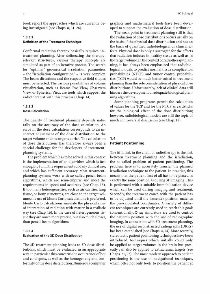
1.3.3.4 Evaluation of the 3D Dose Distribution

The 3D-treatment planning leads to 3D-dose distri-butions, which must be evaluated in an appropriate way. In particular this concerns the occurrence of hot and cold spots, as well as the homogeneity and con-formity of the dose distribution. Numerous computer

graphics and mathematical tools have been devel-oped to support the evaluation of dose distribution.

The weak point in treatment planning still is that the evaluation of dose distributions occurs usually on the basis of the physical dose distribution and not on the basis of quantifi ed radiobiological or clinical ef-fects. Physical dose is only a surrogate for the effects that radiation induces in healthy tissue as well as in the target volume. In the context of radiotherapy plan-ning, it has always been emphasized that radiobio-logical models to predict normal tissue complication probabilities (NTCP) and tumor control probabili-ties (TCP) would be much better suited to treatment planning than the sole consideration of physical dose distributions. Unfortunately, lack of clinical data still hinders the development of adequate biological plan-ning algorithms.

Some planning programs permit the calculation of values for the TCP and for the NTCP as yardsticks for the biological effect of the dose distribution; however, radiobiological models are still the topic of much controversial discussion (see Chap. 18).

1.4 Patient Positioning

The fi fth link in the chain of radiotherapy is the link between treatment planning and the irradiation, the so-called problem of patient positioning. The problem here is to accurately transfer the planned irradiation technique to the patient. In practice, this means that the patient fi rst of all has to be placed in exactly the same position as during 3D imaging. This is performed with a suitable immobilization device which can be used during imaging and treatment. Secondly, the treatment couch with the patient has to be adjusted until the isocenter position matches the pre-calculated coordinates. A variety of differ-ent techniques are currently used to reach this goal: conventionally, X-ray simulators are used to control the patient’s position with the use of radiographic imaging. In connection with 3D-treatment planning, the use of digital reconstructed radiographs (DRRs) has been established (see Chaps. 4, 14). More recently, stereotactic patient positioning techniques have been introduced, techniques which initially could only be applied to target volumes in the brain but pres-ently can also be applied to extracranial targets (see Chaps. 21, 22). The most modern approach to patient positioning is the use of navigational techniques, which offer not only tools to position the patient at

New Technologies in 3D Conformal Radiation Therapy: Introduction and Overview 5

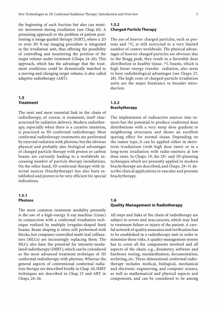
the beginning of each fraction but also can moni-tor movement during irradiation (see Chap. 26). A promising approach to the problem of patient posi-tioning is image-guided therapy (IGRT), where a 2D or even 3D X-ray imaging procedure is integrated in the irradiation unit, thus offering the possibility of controlling and monitoring the position of the target volume under treatment (Chaps. 24–26). This approach, which has the advantage that the treat-ment conditions could be dynamically matched to a moving and changing target volume, is also called adaptive radiotherapy (ART).

1.5 Treatment

The next and most essential link in the chain of radiotherapy, of course, is treatment, itself char-acterized by radiation delivery. Modern radiother-apy, especially when there is a curative intention, is practiced as 3D conformal radiotherapy. Most conformal radiotherapy treatments are performed by external radiation with photons, but the obvious physical and probably also biological advantages of charged particle therapy with proton or carbon beams are currently leading to a worldwide in-creasing number of particle-therapy installations. On the other hand, 3D conformal therapy with in-ternal sources (brachytherapy) has also been es-tablished and proven to be very efficient for special indications.

1.5.1 Photons

The most common treatment modality presently is the use of a high-energy X-ray machine (Linac) in conjunction with a conformal irradiation tech-nique realized by multiple irregular-shaped fi xed beams. Beam shaping is often still performed with blocks, but computer-controlled multi-leaf collima-tors (MLCs) are increasingly replacing them. The MLCs also have the potential for intensity-modu-lated radiotherapy (IMRT), which can be considered as the most advanced treatment technique of 3D conformal radiotherapy with photons. Whereas the general aspects of conventional conformal radia-tion therapy are described briefl y in Chap. 20, IMRT techniques are described in Chap. 23 and ART in Chaps. 24–26.

1.5.2 Charged-Particle Therapy

The use of heavier charged particles, such as pro-tons and 12C, is still restricted to a very limited number of centers worldwide. The physical advan-tages of heavier charged particles are obvious: due to the Bragg peak, they result in a favorable dose distribution in healthy tissue. 12C beams, which is high linear energy transfer radiation, also seem to have radiobiological advantages (see Chaps. 27, 28). The high costs of charged-particle irradiation units are the major hindrance to broader intro-duction.

1.5.3 Brachytherapy

The implantation of radioactive sources into tu-mors has the potential to produce conformal dose distributions with a very steep dose gradient to neighboring structures and shows an excellent sparing effect for normal tissue. Depending on the tumor type, it can be applied either in short-term irradiations (with high dose rates) or in a long-term irradiation with radio-emitters at low dose rates. In Chaps. 19, the 2D- and 3D-planning techniques which are presently applied in modern brachytherapy are described, and Chaps. 29–31 de-scribe clinical applications in vascular and prostate brachytherapy.

1.6 Quality Management in Radiotherapy

All steps and links of the chain of radiotherapy are subject to errors and inaccuracies, which may lead to treatment failure or injury of the patient. A care-ful network of quality assurance and verifi cation has to be established in a radiotherapy unit in order to minimize these risks. A quality management system has to cover all the components involved and all aspects of the chain, e.g., dosimetry, software and hardware testing, standardization, documentation, archiving, etc. Three-dimensional conformal radio-therapy includes medical, biological, mechanical and electronic engineering, and computer science, as well as mathematical and physical aspects and components, and can be considered to be among

6 W. Schlegel

the most complex and critical medical treatment techniques currently available. For this reason, ef-fi cient quality management is an indispensable re-quirement for modern 3D conformal radiotherapy (see Chaps. 32, 33).

References

Schlegel W, Mahr A (2001) 3D conformal radiotherapy: intro-duction to methods and techniques. Springer, Berlin Hei-delberg NewYork

3D Reconstruction 7

Basics of 3D Imaging

3D Reconstruction 9

2 3D Reconstruction

Jürgen Hesser and Dzmitry Stsepankou

J. Hesser, PhD, ProfessorD. StsepankouDepartment of ICM, Universitäten Mannheim und Heidelberg, B6, 23–29, C, 68131 Mannheim, Germany

Röntgen’s contribution to X-ray imaging is a little over 100 years old. Although there was early interest in the extension of the technique to three dimensions, it took more than 70 years for a fi rst prototype. Since then, both the scanner technology, reconstruction al-gorithm, and computer performance have been de-veloped so signifi cantly that in the near future we can expect new techniques with suppressed artefacts in the images. Current developments of such methods are discussed in this chapter.

2.1 Problem Setting

We begin with a presentation of the inverse problem: Given a set of X-ray projections p of an object, try to compute the distribution of attenuation coeffi cients

µ in this object. We can defi ne the projection func-tion P: p=P(µ). Formally, reconstruction is therefore the calculation of an inverse of P, i.e. µ=P–1(p). This inverse need not necessarily exist or, even if it does exist, it may be unstable in the sense that small errors in the projection data can lead to large deviations in the reconstruction.

In order to determine the projection function P we have to look at the physical imaging process more closely. X-ray projection follows the Lambert-Beer law. It describes the attenuation of X-rays penetrat-ing an object with absorption coeffi cient µ and thick-ness d. A ray with initial intensity I0 is attenuated to I = I0e–µd. If the object’s attenuation varies along the ray, one can write I = I0e–∫µ(x)dx, where the integral is along the path the ray passes through the object. We divide by I0 and take the negative logarithm: p = –ln (I/I0) = Úµ(x)dx. Let u(x) describe the contribu-tion of each volume element (infi nitely small cube) to the absorption of the considered ray, the inte-gral can be written as p = Ú

volume µ(x)u(x)dx, where the

integration is now over the full volume. Discretizing the volume, we consider homogenous small cubes with a non-vanishing size, each having an absorp-tion coeffi cient µi ; thus, the integral is replaced by a sum reading: p = ∑

i µi ui , where ui is a weighting factor.

Solving for µi requires a set of such equations being independent of each other; therefore, n projections of size m2 result in n · m2 different rays. For each of them pj = ∑

i µi uij which can be rewritten in vector

format pÆ = U µÆ . pÆ describes all n · m2 different rays, µÆ represents the absorption coeffi cients for all dis-crete volume elements and matrix element (U)ij = uij says how much a volume element i contributes to the projection result of ray j, i.e. all what we have to do is to invert this set of equations, namely µÆ = U–1 pÆ .

Under certain restrictions imposed on the pro-jection directions this set of equations is solvable, i.e. U–1 exists. A direct calculation of the inverse of the matrix U, however, is impossible for present-day computers due to the extraordinary large number of more than 107 variables for typical problems. The following methods are, therefore,

CONTENTS

2.1 Problem Setting 92.2 Parallel-Beam Reconstruction Using the Fourier- Slice Theorem 102.3 Fan-Beam Reconstruction 102.4 Reconstruction Methods of Spiral CT 112.5 Cone-Beam Reconstruction 112.5.1 Exact Methods 112.5.2 Filtered Backprojection for Cone Beams 112.6 Iterative Approaches 122.6.1 Algebraic Reconstruction Techniques 122.6.2 Expectation Maximization Technique 132.7 Regularization Techniques 142.8 Hardware Acceleration 142.8.1 Parallelization 142.8.2 Field Programmable Gate Arrays 142.8.3 Graphics Accelerators 142.9 Outlook 15 References 15

10 J. Hesser and D. Stsepankou

techniques that allow solving such systems more efficiently.

2.2 Parallel-Beam Reconstruction Using the Fourier-Slice Theorem

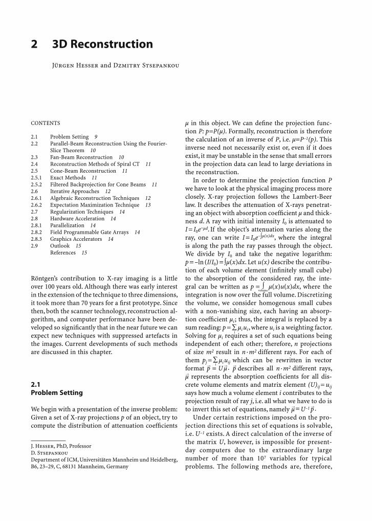
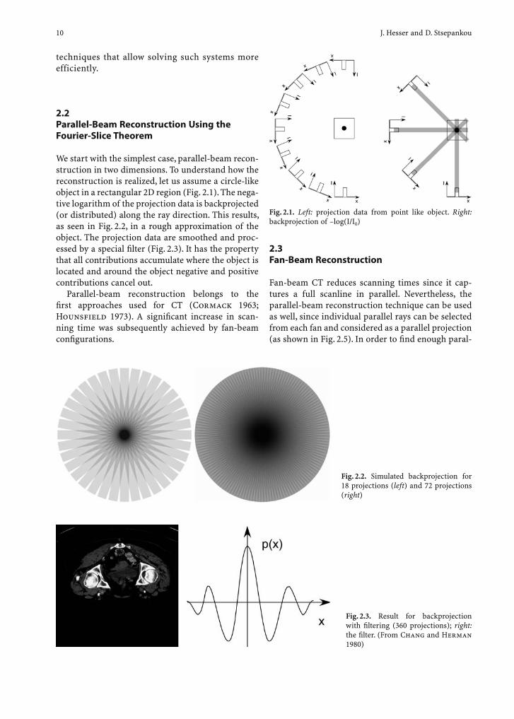
We start with the simplest case, parallel-beam recon-struction in two dimensions. To understand how the reconstruction is realized, let us assume a circle-like object in a rectangular 2D region (Fig. 2.1). The nega-tive logarithm of the projection data is backprojected (or distributed) along the ray direction. This results, as seen in Fig. 2.2, in a rough approximation of the object. The projection data are smoothed and proc-essed by a special fi lter (Fig. 2.3). It has the property that all contributions accumulate where the object is located and around the object negative and positive contributions cancel out.

Parallel-beam reconstruction belongs to the fi rst approaches used for CT (Cormack 1963; Hounsfi eld 1973). A signifi cant increase in scan-ning time was subsequently achieved by fan-beam confi gurations.

2.3 Fan-Beam Reconstruction

Fan-beam CT reduces scanning times since it cap-tures a full scanline in parallel. Nevertheless, the parallel-beam reconstruction technique can be used as well, since individual parallel rays can be selected from each fan and considered as a parallel projection (as shown in Fig. 2.5). In order to fi nd enough paral-

Fig. 2.1. Left: projection data from point like object. Right: backprojection of –log(I/I0)

Fig. 2.2. Simulated backprojection for 18 projections (left) and 72 projections (right)

Fig. 2.3. Result for backprojection with fi ltering (360 projections); right: the fi lter. (From Chang and Herman 1980)

3D Reconstruction 11

lel rays, a suffi cient number of projections covering 180°+ fan-beam angle is required.

Fan-beam CT was used for a long time until in the 1990s KALENDER invented the spiral CT, i.e. a fan-beam CT where the table is shifted with constant speed through the gantry so that the X-ray source follows a screw line around the patient (Kalender et al. 1990).

2.4 Reconstruction Methods of Spiral CT

For spiral CT the projection lines do not lie in paral-lel planes as for fan-beam CT. Linear interpolation of the captured data on parallel planes allows use of the fan-beam reconstruction method. Data required for interpolation may come from either projections being 360 or 180° apart where the latter yields a bet-ter resolution.

In recent years, CT exams with several detector lines have been introduced reducing the overall scan-ning time for whole-body scans. Despite the diver-gence of the rays in different detector rows, standard reconstruction techniques are used. Recently, further developments have reconstructed optimally adapted oblique reconstruction planes that are later interpo-lated into a set of parallel slices (Kachelriess et al. 2000).

2.5 Cone-Beam Reconstruction

For cone-beam reconstruction we differentiate be-tween exact methods, direct approximations, and iterative approximations.

2.5.1 Exact Methods

Exact reconstruction algorithms have been devel-oped (Grangeat 1991; Defrise and Clack 1994; Kudo and Saito 1994), but they currently do not play a role in practice due to the long reconstruction time and high memory consumption. Cone-beam recon-struction imposes constraints on the motion of the source-detector combination around the patient. As shown in Fig. 2.6, a pure rotation around the patient does not deliver information about all regions and therefore a correct reconstruction is not possible; however, trajectories, as shown in Fig. 2.7, for exam-ple, solve this problem (Tam et al. 1998).

2.5.2 Filtered Backprojection for Cone Beams

In fi ltered backprojection (FBP) the projection data is fi ltered with an appropriate fi lter mask, backprojected and fi nally accumulated (Feldkamp et al. 1984; Yan and Leahy 1992; Schaller et al. 1997). For small cone-beam angles fairly good results are obtained, but for larger angles the conditions for parallel beams are violated leading to typical artefacts. Nevertheless, fi ltered backprojection is currently the standard for commercial cone-beam systems (Euler et al. 2000). From the computational point of view, FBP is more time-consuming compared with the parallel beam, fan beam, or spiral reconstruction since the latter use the Fourier transform to solve backprojection

Fig. 2.4. Results on simulated data. Shepp-Logan phantom (Shepp and Logan 1974; left), fi ltered backprojection result for 360 projections (right)

Fig. 2.5. Three different fan-beam projections are shown [shown as triangles with different colours; circles denote the X-ray sources (1–3)]. We identify three approximately parallel rays in the three projections shown as green, violet, and blue. These could be interpreted as a selection of three rays of a parallel projection arrangement.

12 J. Hesser and D. Stsepankou

fast. Although fast FBP implementations exist (Toft 1996), they do not reach a similar reconstruction quality.

2.6 Iterative Approaches

Filtered backprojection can be characterized as an example of direct inversion techniques. For partic-ularly good reconstruction quality FBP is not the method of choice since it can produce severe artefacts especially in the case of the presence of high-contrast objects or a small number of projection data. Iterative techniques promise better reconstructions.

2.6.1 Algebraic Reconstruction Techniques

The algebraic reconstruction technique (ART; Gordon et al. 1970) is one of the fi rst approaches to solve the reconstruction problem using an iterative method. The basic idea is to start with an a priori guess about the density distribution. The density is often assumed to be zero everywhere. Next, the simu-

Fig. 2.6. Using only a circular path about the object, one is not able to reconstruct parts of the volume.

Fig. 2.7. Source detector motion that allows reconstructing the volume for cone beam confi gurations

Fig. 2.8 Result of a reconstruction using fi ltered backprojection. One hundred twenty projections of size 512×512

3D Reconstruction 13

lated projection is calculated and compared with the acquired projection data. The error is backprojected (without fi ltering) and then accumulated from each projection leading to an improved guess. Iteratively applying this course of simulated projection, error calculation and error backprojection, the algorithm converges towards the most likely solution.

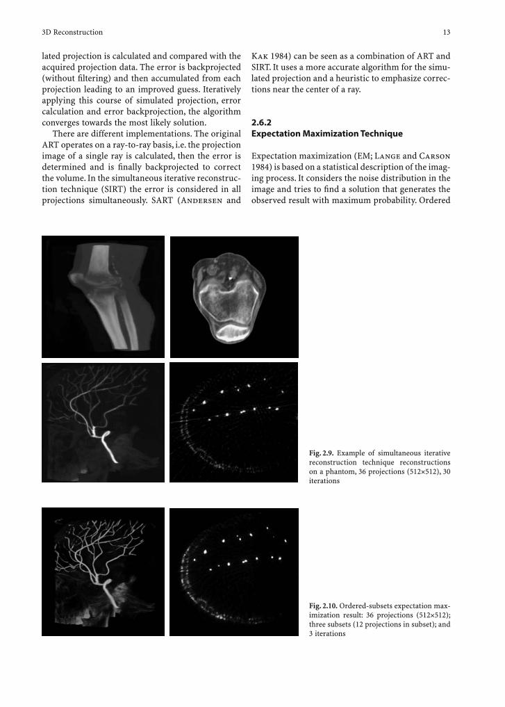
There are different implementations. The original ART operates on a ray-to-ray basis, i.e. the projection image of a single ray is calculated, then the error is determined and is fi nally backprojected to correct the volume. In the simultaneous iterative reconstruc-tion technique (SIRT) the error is considered in all projections simultaneously. SART (Andersen and

Kak 1984) can be seen as a combination of ART and SIRT. It uses a more accurate algorithm for the simu-lated projection and a heuristic to emphasize correc-tions near the center of a ray.

2.6.2 Expectation Maximization Technique

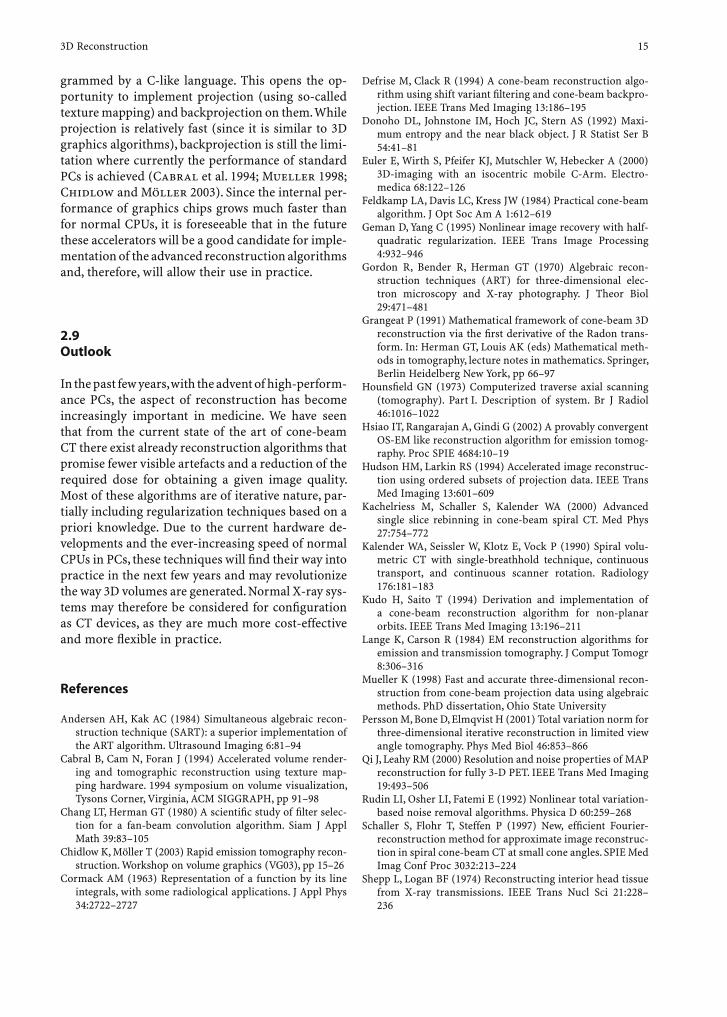
Expectation maximization (EM; Lange and Carson 1984) is based on a statistical description of the imag-ing process. It considers the noise distribution in the image and tries to fi nd a solution that generates the observed result with maximum probability. Ordered

Fig. 2.9. Example of simultaneous iterative reconstruction technique reconstructions on a phantom, 36 projections (512×512), 30 iterations

Fig. 2.10. Ordered-subsets expectation max-imization result: 36 projections (512×512); three subsets (12 projections in subset); and 3 iterations

14 J. Hesser and D. Stsepankou

subset methods where a subset of all projections for each iteration step is chosen (Hudson and Larkin 1994; Hsiao et al. 2002) can speed up convergence by a factor of approximately 10, although this is not as fast as SIRT or SART.

2.7 Regularization Techniques

Iterative approaches, at best, yield a maximum-likeli-hood solution. This is a solution, given only the in-formation about the physical process of imaging and the data, which describes the most probable density distribution of physical parameters. In many cases, however, one has additional knowledge about the ob-ject to be imaged. For example, restrictions can be imposed on the size of the object and the maximal, minimal or average X-ray density; there may also be an a priori data set, etc. Including this information in the reconstruction process can substantially increase the reconstruction quality and accuracy.

Let us refer to the reconstruction problem as de-scribed above: Given the function (matrix) that de-scribes the physical imaging process, U, fi nd the den-sity distribution µÆ so that the error E(µÆ )=( µÆ – U pÆ )2 is minimal. This is the least-square approximation. A regularization modifi es this function by adding a regularization function R(µÆ): E(µÆ) = ( pÆ – U µÆ)2+aR(µÆ), where a is a coupling constant that has to be chosen manually.

Finding suited regularization functions is a diffi -cult task (YU and Fessler 2002). Simple examples are Tikhonov regularizations (Tikhonov et al. 1997), where R(µÆ) has been chosen as the scalar product [L(µ-µ*)]·[L(µ-µ*)], where L is typically either the identity matrix or the discrete approximation of the derivative operator and µ* is the a priori distribution of the absorption coeffi cient. More advanced and re-cent techniques are impulse-noise priors (Donoho et al. 1992; Qi and Leahy 2000), Markov random-fi elds priors (Geman and Yang 1995; Villain et al. 2003) and total variation regularization (Rudin et al. 1992; Persson et al. 2001).

2.8 Hardware Acceleration

2.8.1 Parallelization

One of the signifi cant disadvantages of the cone-beam reconstruction technique is the high compu-tational demands preventing use in daily practice; therefore, parallelization has been a natural means for acceleration. The naive approach is to subdivide the volume into small subvolumes, assign each sub-volume to one processor and then compute simulated projection and backprojection locally. Since the pro-jection result is combined by the partial projection results from all subvolumes, processors have to send their intermediate results to a central node where the fi nal projection is generated and then distributed to all other processors again. Current parallel comput-ers are generally limited for this sort of processing by their network bandwidth. In other words, the proc-essors process the data faster than the network can transmit the results to other processors; therefore, parallelization is not very attractive. There are, how-ever, two new upcoming technologies that promise a solution.

2.8.2 Field Programmable Gate Arrays

Field programmable gate arrays are chips where the internal structure can be confi gured to any hardware logic, e.g. some sort of CPU or, which is interesting in our application, to a special-purpose processor. The main advantage is that recent chips have hundreds of multipliers and several million logic elements that can be confi gured as switches, adders or memory. Recently, it has been demonstrated that these systems can be more than ten times faster than a normal PC for backprojection, and this factor will grow over the next few years since the amount of computing resources grows faster than the performance of CPUs (Stsepankou et al. 2003).

2.8.3 Graphics Accelerators

Graphics cards contain special-purpose processors optimized for 3D graphics and that internally have the processing power which is much higher than that of normal PCs. Internal graphics can now be pro-

3D Reconstruction 15

grammed by a C-like language. This opens the op-portunity to implement projection (using so-called texture mapping) and backprojection on them. While projection is relatively fast (since it is similar to 3D graphics algorithms), backprojection is still the limi-tation where currently the performance of standard PCs is achieved (Cabral et al. 1994; Mueller 1998; Chidlow and Möller 2003). Since the internal per-formance of graphics chips grows much faster than for normal CPUs, it is foreseeable that in the future these accelerators will be a good candidate for imple-mentation of the advanced reconstruction algorithms and, therefore, will allow their use in practice.

2.9 Outlook

In the past few years, with the advent of high-perform-ance PCs, the aspect of reconstruction has become increasingly important in medicine. We have seen that from the current state of the art of cone-beam CT there exist already reconstruction algorithms that promise fewer visible artefacts and a reduction of the required dose for obtaining a given image quality. Most of these algorithms are of iterative nature, par-tially including regularization techniques based on a priori knowledge. Due to the current hardware de-velopments and the ever-increasing speed of normal CPUs in PCs, these techniques will fi nd their way into practice in the next few years and may revolutionize the way 3D volumes are generated. Normal X-ray sys-tems may therefore be considered for confi guration as CT devices, as they are much more cost-effective and more fl exible in practice.

References

Andersen AH, Kak AC (1984) Simultaneous algebraic recon-struction technique (SART): a superior implementation of the ART algorithm. Ultrasound Imaging 6:81–94

Cabral B, Cam N, Foran J (1994) Accelerated volume render-ing and tomographic reconstruction using texture map-ping hardware. 1994 symposium on volume visualization, Tysons Corner, Virginia, ACM SIGGRAPH, pp 91–98

Chang LT, Herman GT (1980) A scientifi c study of fi lter selec-tion for a fan-beam convolution algorithm. Siam J Appl Math 39:83–105

Chidlow K, Möller T (2003) Rapid emission tomography recon-struction. Workshop on volume graphics (VG03), pp 15–26

Cormack AM (1963) Representation of a function by its line integrals, with some radiological applications. J Appl Phys 34:2722–2727

Defrise M, Clack R (1994) A cone-beam reconstruction algo-rithm using shift variant fi ltering and cone-beam backpro-jection. IEEE Trans Med Imaging 13:186–195

Donoho DL, Johnstone IM, Hoch JC, Stern AS (1992) Maxi-mum entropy and the near black object. J R Statist Ser B 54:41–81

Euler E, Wirth S, Pfeifer KJ, Mutschler W, Hebecker A (2000) 3D-imaging with an isocentric mobile C-Arm. Electro-medica 68:122–126

Feldkamp LA, Davis LC, Kress JW (1984) Practical cone-beam algorithm. J Opt Soc Am A 1:612–619

Geman D, Yang C (1995) Nonlinear image recovery with half-quadratic regularization. IEEE Trans Image Processing 4:932–946

Gordon R, Bender R, Herman GT (1970) Algebraic recon-struction techniques (ART) for three-dimensional elec-tron microscopy and X-ray photography. J Theor Biol 29:471–481

Grangeat P (1991) Mathematical framework of cone-beam 3D reconstruction via the fi rst derivative of the Radon trans-form. In: Herman GT, Louis AK (eds) Mathematical meth-ods in tomography, lecture notes in mathematics. Springer, Berlin Heidelberg New York, pp 66–97

Hounsfi eld GN (1973) Computerized traverse axial scanning (tomography). Part I. Description of system. Br J Radiol 46:1016–1022

Hsiao IT, Rangarajan A, Gindi G (2002) A provably convergent OS-EM like reconstruction algorithm for emission tomog-raphy. Proc SPIE 4684:10–19

Hudson HM, Larkin RS (1994) Accelerated image reconstruc-tion using ordered subsets of projection data. IEEE Trans Med Imaging 13:601–609

Kachelriess M, Schaller S, Kalender WA (2000) Advanced single slice rebinning in cone-beam spiral CT. Med Phys 27:754–772

Kalender WA, Seissler W, Klotz E, Vock P (1990) Spiral volu-metric CT with single-breathhold technique, continuous transport, and continuous scanner rotation. Radiology 176:181–183

Kudo H, Saito T (1994) Derivation and implementation of a cone-beam reconstruction algorithm for non-planar orbits. IEEE Trans Med Imaging 13:196–211

Lange K, Carson R (1984) EM reconstruction algorithms for emission and transmission tomography. J Comput Tomogr 8:306–316

Mueller K (1998) Fast and accurate three-dimensional recon-struction from cone-beam projection data using algebraic methods. PhD dissertation, Ohio State University

Persson M, Bone D, Elmqvist H (2001) Total variation norm for three-dimensional iterative reconstruction in limited view angle tomography. Phys Med Biol 46:853–866

Qi J, Leahy RM (2000) Resolution and noise properties of MAP reconstruction for fully 3-D PET. IEEE Trans Med Imaging 19:493–506

Rudin LI, Osher LI, Fatemi E (1992) Nonlinear total variation-based noise removal algorithms. Physica D 60:259–268

Schaller S, Flohr T, Steffen P (1997) New, effi cient Fourier-reconstruction method for approximate image reconstruc-tion in spiral cone-beam CT at small cone angles. SPIE Med Imag Conf Proc 3032:213–224

Shepp L, Logan BF (1974) Reconstructing interior head tissue from X-ray transmissions. IEEE Trans Nucl Sci 21:228–236

16 J. Hesser and D. Stsepankou

Stsepankou D, Müller U, Kornmesser K, Hesser J, Männer R (2003) FPGA-accelerated volume reconstruction from X-ray. World Conference on Medical Physics and Biomedical Engineering, Sydney, Australia

Tam KC, Samarasekera S, Sauer F (1998) Exact cone-beam CT with a spiral scan. Phys Med Biol 43:1015–1024

Tikhonov AN, Leonov AS, Yagola A (1997) Nonlinear ill-posed problems. Kluwer, Dordrecht

Toft P (1996) The radon transform: theory and implementa-tion. PhD thesis, Department of Mathematical Modelling, Technical University of Denmark

Villain N, Goussard Y, Idier J, Allain M (2003) Three-dimensional edge-preserving image enhancement for computed tomography. IEEE Trans Med Imaging 22:1275–1287

Yan XH, Leahy RM (1992) Cone-beam tomography with cir-cular, elliptical, and spiral orbits. Phys Med Biol 37:493–506

Yu DF, Fessler JA (2002) Edge-preserving tomographic recon-struction with nonlocal regularization. IEEE Trans Med Imaging 21:159–173

Processing and Segmentation of 3D Images 17

3 Processing and Segmentation of 3D Images

Georgios Sakas and Andreas Pommert

G. Sakas, PhDFraunhofer Institute for Computer Graphics (IGD), Fraunhoferstrasse 5, 64283 Darmstadt, GermanyA. Pommert, PhDInstitut für Medizinische Informatik (IMI), Universitätsklinikum Hamburg-Eppendorf, Martinistrasse 52, 20246 Hamburg, Germany

3.1 Introduction

For a very long time, ranging approximately from early trepanizations of heads in Neolithic ages until little more than 100 years ago, the basic principles of medical practice did not change signifi cantly. The ap-plication of X-rays for gathering images from the body interior marked a major milestone in the history of medicine and introduced a paradigm change in the way humans understood and practiced medicine.

The revolution introduced by medical imaging is still evolving. After X-rays, several other modalities have been developed allowing us new, different, and more complete views of the body interior: tomogra-phy (CT, MR) gives a very precise anatomically clear view and allows localization in space; nuclear medi-cine gives images of metabolism; ultrasound and in-version recovery imaging enable non-invasive imag-ing; and there are many others.

All these magnifi cent innovations have one thing in common: they provide images as primary informa-tion, thus allowing us to literally “see things” and to capitalize from the unmatched capabilities of our vi-

CONTENTS

3.1 Introduction 173.2 Pre-processing 183.3 Segmentation 203.3.1 Classifi cation 203.3.2 Edge Detection 223.3.3 2.5-D Boundary Tracking 223.3.4 Geodesic Active Contours 233.3.5 Extraction of Tubular Objects 243.3.6 Atlas Registration 243.3.7 Interactive Segmentation 25 References 25

sual system. On the other hand, the increasing number of images produces also a complexity bottleneck: it becomes continuously more and more diffi cult to han-dle, correlate, understand, and archive all the different views delivered by the various imaging modalities.

Computer graphics as an enabling technology is the key and the answer to this problem. With increas-ing power of even moderate desktop computers, the present imaging methods are able to handle the com-plexity and huge data volume generated by these im-aging modalities.

While in the past images were typically two-di-mensional – be they X-rays, CT slices or ultrasound scans – there has been a shift towards reproducing the three-dimensionality of human organs. This trend has been supported above all by the new role of surgeons as imaging users who, unlike radiologists (who have practiced “abstract 2D thinking” for years), must fi nd their way around complicated structures and navigate within the body (Hildebrand et al. 1996).

Modern computers are used to generate 3D recon-structions of organs using 2D data. Increasing computer power, falling prices, and general availability have al-ready established such systems as the present standard in medicine. Legislators have also recognized this fact. In the future, medical software may be used (e.g. com-mercially sold) in Europe only if it displays a CE mark in compliance with legal regulations (MDD, MPG). To this end, developers and manufacturers must carry out a risk analysis in accordance with EN 60601-1-4 and must validate their software. As soon as software is used with humans, this is true also for research groups, who desire to disseminate their work for clinical use, even if they do not have commercial ambitions.

The whole process leading from images to 3D views can be organized as a pipeline. An overview of the volume visualization pipeline as presented in this chapter and in Chap. 4 is shown in Fig. 3.1. After the acquisition of one or more series of tomographic im-ages, the data usually undergo some pre-processing such as image fi ltering, interpolation, and image fu-sion, if data from several sources are to be used. From this point, one of several paths may be followed.

18 G. Sakas and A. Pommert

The more traditional surface-extraction methods fi rst create an intermediate surface representation of the objects to be shown. It can then be rendered with any standard computer-graphics utilities. More recently, di-rect volume-visualization methods have been developed which create 3D views directly from the volume data. These methods use the full image intensity informa-tion (gray levels) to render surfaces, cuts, or transparent and semi-transparent volumes. They may or may not include an explicit segmentation step for the identifi ca-tion and labeling of the objects to be rendered.

Extensions to the volume visualization pipeline not shown in Fig. 3.1, but covered herein, include the visualization of transformed data and intelligent vi-sualization.

3.2 Pre-processing

The data we consider usually comes as a spatial se-quence of 2D cross-sectional images. When they are put on top of each other, a contiguous image volume is obtained. The resulting data structure is an orthogonal 3D array of volume elements or voxels each represent-ing an intensity value, equivalent to picture elements or pixels in 2D. This data structure is called the voxel

model. In addition to intensity information, each voxel may also contain labels, describing its membership to various objects, and/or data from different sources (generalized voxel model; Höhne et al. 1990).

Many algorithms for volume visualization work on isotropic volumes where the voxel spacing is equal in all three dimensions. In practice, however, only very few data sets have this property, especially for CT. In these cases, the missing information has to be approximated in an interpolation step. A very simple method is linear interpolation of the intensities be-tween adjacent images. Higher-order functions, such as splines, usually yield better results for fi ne details (Marschner and Lobb 1994; Möller et al. 1997).

In windowing techniques only a part of the image depth values is displayed with the available gray val-ues. The term “window” refers to the range of CT num-bers which are displayed each time (Hemmingsson et al. 1980; Warren et al. 1982). This window can be moved along the whole range of depth values of the image, displaying each time different tissue types in the full range of the gray scale achieving this way bet-ter image contrast and/or focusing on material with specifi c characteristics (Fig. 3.2). The new brightness value of the pixel Gv is given by the formula:

minminmax )( GvWsWl

WsWeGvGvGv +−⋅⎟

⎠⎞

⎜⎝⎛

−−

=

Fig. 3.1. The general organisation of processing, segmentation and visualisation steps

Patient

3D Images

Processing and Segmentation of 3D Images 19

where [Gvmax, Gvmin], is the gray-level range, [Ws, We] defi nes the window width, and Wl the window center. This is the simplest case of image windowing. Often, depending on the application, the window might have more complicated forms such as double window, bro-ken window, or non-linear windows (exponential or sinusoid or the like).

The sharpening when applied to an image aims to decrease the image blurring and enhance image edges. Among the most important sharpening meth-ods, high-emphasis masks, unsharp masking, and high-pass fi ltering (Fig. 3.3) should be considered.

There are two ways to apply these fi lters on the im-age: (a) in the spatial domain using the convolution process and the appropriate masks; and (b) in the fre-quency domain using high-pass fi lters.

Generally, fi lters implemented in the spatial do-main are faster and more intuitive to implement, whereas fi lters in the frequency domain require prior transformation of the original, e.g., by means of the Fourier transformation. Frequency domain imple-

mentations offer benefi ts for large data sets (3D vol-umes), whereas special domain implementations are preferred for processing single images.

Image-smoothing techniques are used in image processing to reduce noise. Usually in medical imag-ing the noise is distributed statistically and it exists in high frequencies; therefore, it can be stated that im-age-smoothing fi lters are low-pass fi lters. The draw-back of applying a smoothing fi lter is the simultane-ous reduction of useful information, mainly detail features, which also exist in high frequencies (Sonka et al. 1998).

Typical fi lters (Fig. 3.4) here include averaging masks as well as Gaussian and median fi ltering. Averaging and Gaussian fi ltering tend to reduce the sharpness of edges, whereas median fi lters preserve edge sharpness. Smoothing fi lters are typically imple-mented in the spatial domain.

In MRI, another obstacle may be low-frequency intensity inhomogeneities, which can be corrected to some extent (Arnold et al. 2001).

Fig. 3.2. by applying different windowing techniques different aspects of the same volume can be emphasized

Fig. 3.3. Original CT slice (left) and contour extraction (right)

20 G. Sakas and A. Pommert

3.3 Segmentation

An image volume usually represents a large number of different structures obscuring each other. To dis-play a particular one, we thus have to decide which parts of the volume we want to use or ignore. A fi rst step is to partition the image volume into different re-gions, which are homogeneous with respect to some formal criteria and correspond to real (anatomical) objects. This process is called segmentation. In a subsequent interpretation step, the regions may be identifi ed and labeled with meaningful terms such as “white matter” or “ventricle.” While segmentation is easy for a human expert, it has turned out to be an extremely diffi cult task for the computer.

All segmentation methods can be characterized as being either binary or fuzzy, corresponding to the principles of binary and fuzzy logic, respectively (Winston 1992). In binary segmentation, the ques-tion of whether a voxel belongs to a certain region is always answered by either yes or no. This infor-mation is a prerequisite, e.g., for creating surface representations from volume data. As a drawback, uncertainty or cases where an object takes up only a fraction of a voxel (partial-volume effect) can-not be handled properly. Strict yes/no decisions are avoided in fuzzy segmentation, where a set of probabilities is assigned to every voxel, indicating the evidence for different materials. Fuzzy segmen-tation is closely related to the direct volume-render-ing methods (see below).

Following is a selection of the most common seg-mentation methods used for volume visualization, ranging from classifi cation and edge detection to recent approaches such as snakes, atlas registration, and interactive segmentation. In practice, these basic approaches are often combined. For further read-ing, the excellent survey on medical image analysis (Duncan and Ayache 2000) is recommended.

3.3.1 Classifi cation

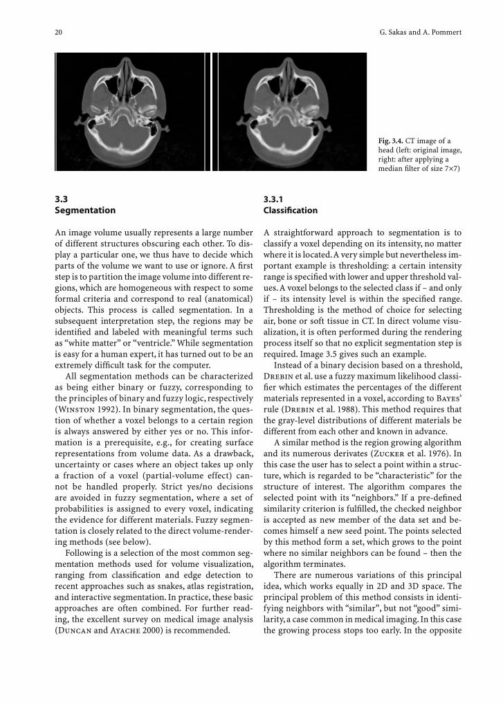
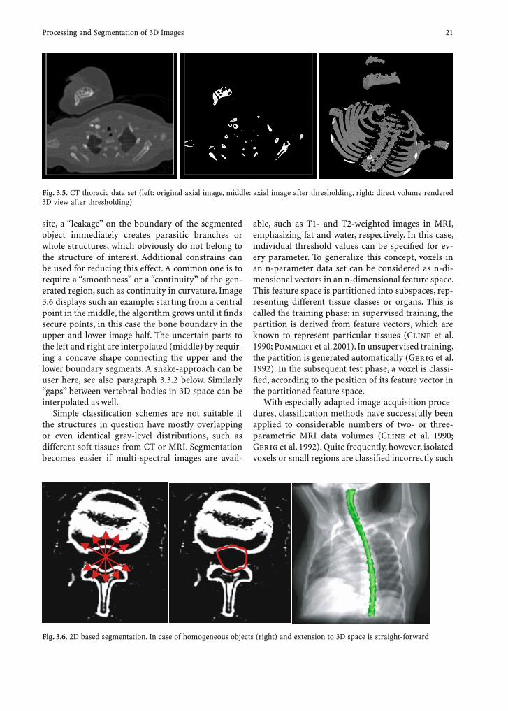
A straightforward approach to segmentation is to classify a voxel depending on its intensity, no matter where it is located. A very simple but nevertheless im-portant example is thresholding: a certain intensity range is specifi ed with lower and upper threshold val-ues. A voxel belongs to the selected class if – and only if – its intensity level is within the specifi ed range. Thresholding is the method of choice for selecting air, bone or soft tissue in CT. In direct volume visu-alization, it is often performed during the rendering process itself so that no explicit segmentation step is required. Image 3.5 gives such an example.

Instead of a binary decision based on a threshold, Drebin et al. use a fuzzy maximum likelihood classi-fi er which estimates the percentages of the different materials represented in a voxel, according to Bayes’ rule (Drebin et al. 1988). This method requires that the gray-level distributions of different materials be different from each other and known in advance.

A similar method is the region growing algorithm and its numerous derivates (Zucker et al. 1976). In this case the user has to select a point within a struc-ture, which is regarded to be “characteristic” for the structure of interest. The algorithm compares the selected point with its “neighbors.” If a pre-defi ned similarity criterion is fulfi lled, the checked neighbor is accepted as new member of the data set and be-comes himself a new seed point. The points selected by this method form a set, which grows to the point where no similar neighbors can be found – then the algorithm terminates.

There are numerous variations of this principal idea, which works equally in 2D and 3D space. The principal problem of this method consists in identi-fying neighbors with “similar”, but not “good” simi-larity, a case common in medical imaging. In this case the growing process stops too early. In the opposite

Fig. 3.4. CT image of a head (left: original image, right: after applying a median fi lter of size 7¥7)

Processing and Segmentation of 3D Images 21

site, a “leakage” on the boundary of the segmented object immediately creates parasitic branches or whole structures, which obviously do not belong to the structure of interest. Additional constrains can be used for reducing this effect. A common one is to require a “smoothness” or a “continuity” of the gen-erated region, such as continuity in curvature. Image 3.6 displays such an example: starting from a central point in the middle, the algorithm grows until it fi nds secure points, in this case the bone boundary in the upper and lower image half. The uncertain parts to the left and right are interpolated (middle) by requir-ing a concave shape connecting the upper and the lower boundary segments. A snake-approach can be user here, see also paragraph 3.3.2 below. Similarly “gaps” between vertebral bodies in 3D space can be interpolated as well.

Simple classifi cation schemes are not suitable if the structures in question have mostly overlapping or even identical gray-level distributions, such as different soft tissues from CT or MRI. Segmentation becomes easier if multi-spectral images are avail-

able, such as T1- and T2-weighted images in MRI, emphasizing fat and water, respectively. In this case, individual threshold values can be specifi ed for ev-ery parameter. To generalize this concept, voxels in an n-parameter data set can be considered as n-di-mensional vectors in an n-dimensional feature space. This feature space is partitioned into subspaces, rep-resenting different tissue classes or organs. This is called the training phase: in supervised training, the partition is derived from feature vectors, which are known to represent particular tissues (Cline et al. 1990; Pommert et al. 2001). In unsupervised training, the partition is generated automatically (Gerig et al. 1992). In the subsequent test phase, a voxel is classi-fi ed, according to the position of its feature vector in the partitioned feature space.

With especially adapted image-acquisition proce-dures, classifi cation methods have successfully been applied to considerable numbers of two- or three-parametric MRI data volumes (Cline et al. 1990; Gerig et al. 1992). Quite frequently, however, isolated voxels or small regions are classifi ed incorrectly such

Fig. 3.5. CT thoracic data set (left: original axial image, middle: axial image after thresholding, right: direct volume rendered 3D view after thresholding)

Fig. 3.6. 2D based segmentation. In case of homogeneous objects (right) and extension to 3D space is straight-forward

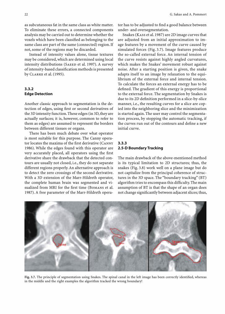
22 G. Sakas and A. Pommert

as subcutaneous fat in the same class as white matter. To eliminate these errors, a connected components analysis may be carried out to determine whether the voxels which have been classifi ed as belonging to the same class are part of the same (connected) region. If not, some of the regions may be discarded.

Instead of intensity values alone, tissue textures may be considered, which are determined using local intensity distributions (Saeed et al. 1997). A survey of intensity-based classifi cation methods is presented by Clarke et al. (1995).

3.3.2 Edge Detection

Another classic approach to segmentation is the de-tection of edges, using fi rst or second derivatives of the 3D intensity function. These edges (in 3D, they are actually surfaces; it is, however, common to refer to them as edges) are assumed to represent the borders between different tissues or organs.

There has been much debate over what operator is most suitable for this purpose. The Canny opera-tor locates the maxima of the fi rst derivative (Canny 1986). While the edges found with this operator are very accurately placed, all operators using the fi rst derivative share the drawback that the detected con-tours are usually not closed, i.e., they do not separate different regions properly. An alternative approach is to detect the zero crossings of the second derivative. With a 3D extension of the Marr-Hildreth operator, the complete human brain was segmented and vi-sualized from MRI for the fi rst time (Bomans et al. 1987). A free parameter of the Marr-Hildreth opera-

tor has to be adjusted to fi nd a good balance between under- and oversegmentation.

Snakes (Kass et al. 1987) are 2D image curves that are adjusted from an initial approximation to im-age features by a movement of the curve caused by simulated forces (Fig. 3.7). Image features produce the so-called external force. An internal tension of the curve resists against highly angled curvatures, which makes the Snakes’ movement robust against noise. After a starting position is given, the snake adapts itself to an image by relaxation to the equi-librium of the external force and internal tension. To calculate the forces an external energy has to be defi ned. The gradient of this energy is proportional to the external force. The segmentation by Snakes is due to its 2D defi nition performed in a slice-by-slice manner, i.e., the resulting curves for a slice are cop-ied into the neighboring slice and the minimization is started again. The user may control the segmenta-tion process, by stopping the automatic tracking, if the curves run out of the contours and defi ne a new initial curve.

3.3.3 2.5-D Boundary Tracking

The main drawback of the above-mentioned method is its typical limitation to 2D structures; thus, the snakes (Fig. 3.8) work well on a plane image but do not capitalize from the principal coherence of struc-tures in the 3D space. The “boundary tracking” (BT) algorithm tries to encompass this diffi culty. The main assumption of BT is that the shape of an organ does not change signifi cantly between adjacent slices; thus,

Fig. 3.7. The principle of segmentation using Snakes. The spinal canal in the left image has been correctly identifi ed, whereas in the middle and the right examples the algorithm tracked the wrong boundary!

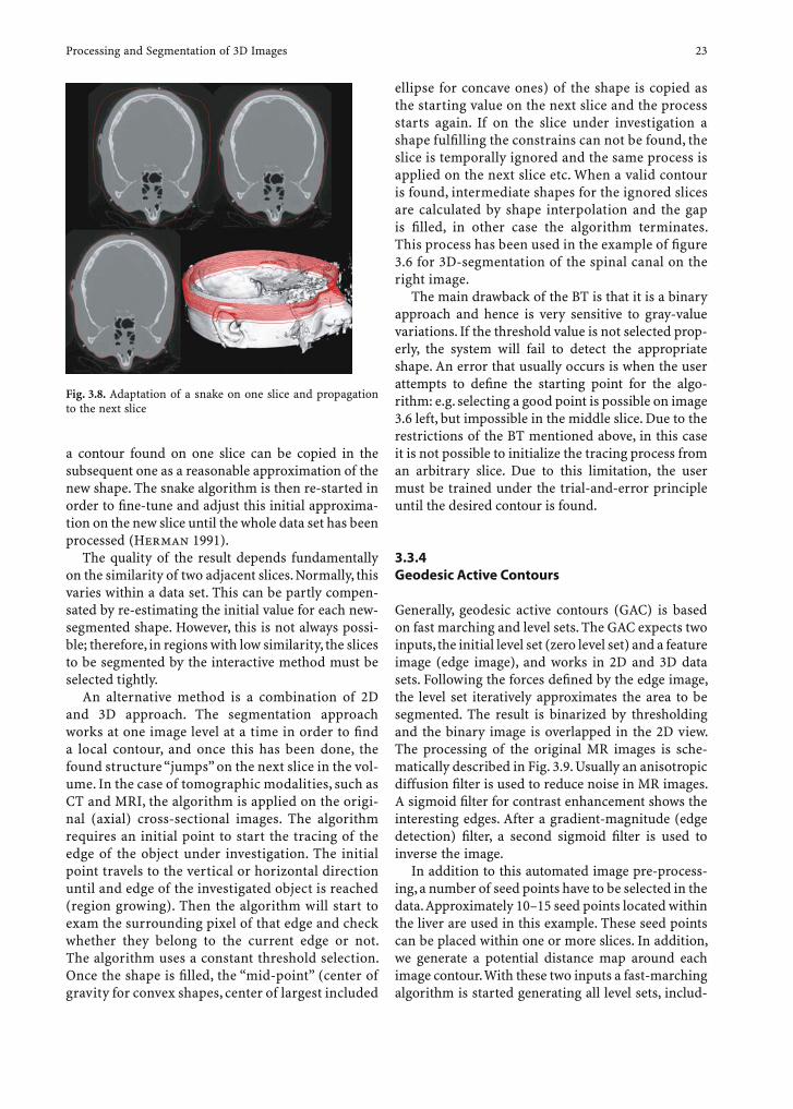
Processing and Segmentation of 3D Images 23

a contour found on one slice can be copied in the subsequent one as a reasonable approximation of the new shape. The snake algorithm is then re-started in order to fi ne-tune and adjust this initial approxima-tion on the new slice until the whole data set has been processed (Herman 1991).

The quality of the result depends fundamentally on the similarity of two adjacent slices. Normally, this varies within a data set. This can be partly compen-sated by re-estimating the initial value for each new-segmented shape. However, this is not always possi-ble; therefore, in regions with low similarity, the slices to be segmented by the interactive method must be selected tightly.

An alternative method is a combination of 2D and 3D approach. The segmentation approach works at one image level at a time in order to fi nd a local contour, and once this has been done, the found structure “jumps” on the next slice in the vol-ume. In the case of tomographic modalities, such as CT and MRI, the algorithm is applied on the origi-nal (axial) cross-sectional images. The algorithm requires an initial point to start the tracing of the edge of the object under investigation. The initial point travels to the vertical or horizontal direction until and edge of the investigated object is reached (region growing). Then the algorithm will start to exam the surrounding pixel of that edge and check whether they belong to the current edge or not. The algorithm uses a constant threshold selection. Once the shape is fi lled, the “mid-point” (center of gravity for convex shapes, center of largest included

ellipse for concave ones) of the shape is copied as the starting value on the next slice and the process starts again. If on the slice under investigation a shape fulfi lling the constrains can not be found, the slice is temporally ignored and the same process is applied on the next slice etc. When a valid contour is found, intermediate shapes for the ignored slices are calculated by shape interpolation and the gap is fi lled, in other case the algorithm terminates. This process has been used in the example of fi gure 3.6 for 3D-segmentation of the spinal canal on the right image.

The main drawback of the BT is that it is a binary approach and hence is very sensitive to gray-value variations. If the threshold value is not selected prop-erly, the system will fail to detect the appropriate shape. An error that usually occurs is when the user attempts to defi ne the starting point for the algo-rithm: e.g. selecting a good point is possible on image 3.6 left, but impossible in the middle slice. Due to the restrictions of the BT mentioned above, in this case it is not possible to initialize the tracing process from an arbitrary slice. Due to this limitation, the user must be trained under the trial-and-error principle until the desired contour is found.

3.3.4 Geodesic Active Contours

Generally, geodesic active contours (GAC) is based on fast marching and level sets. The GAC expects two inputs, the initial level set (zero level set) and a feature image (edge image), and works in 2D and 3D data sets. Following the forces defi ned by the edge image, the level set iteratively approximates the area to be segmented. The result is binarized by thresholding and the binary image is overlapped in the 2D view. The processing of the original MR images is sche-matically described in Fig. 3.9. Usually an anisotropic diffusion fi lter is used to reduce noise in MR images. A sigmoid fi lter for contrast enhancement shows the interesting edges. After a gradient-magnitude (edge detection) fi lter, a second sigmoid fi lter is used to inverse the image.

In addition to this automated image pre-process-ing, a number of seed points have to be selected in the data. Approximately 10–15 seed points located within the liver are used in this example. These seed points can be placed within one or more slices. In addition, we generate a potential distance map around each image contour. With these two inputs a fast-marching algorithm is started generating all level sets, includ-

Fig. 3.8. Adaptation of a snake on one slice and propagation to the next slice

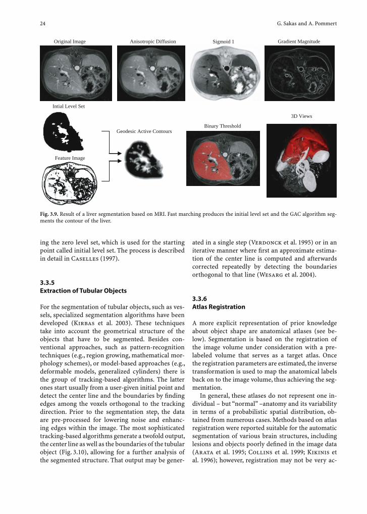
24 G. Sakas and A. Pommert

ing the zero level set, which is used for the starting point called initial level set. The process is described in detail in Caselles (1997).

3.3.5 Extraction of Tubular Objects

For the segmentation of tubular objects, such as ves-sels, specialized segmentation algorithms have been developed (Kirbas et al. 2003). These techniques take into account the geometrical structure of the objects that have to be segmented. Besides con-ventional approaches, such as pattern-recognition techniques (e.g., region growing, mathematical mor-phology schemes), or model-based approaches (e.g., deformable models, generalized cylinders) there is the group of tracking-based algorithms. The latter ones start usually from a user-given initial point and detect the center line and the boundaries by fi nding edges among the voxels orthogonal to the tracking direction. Prior to the segmentation step, the data are pre-processed for lowering noise and enhanc-ing edges within the image. The most sophisticated tracking-based algorithms generate a twofold output, the center line as well as the boundaries of the tubular object (Fig. 3.10), allowing for a further analysis of the segmented structure. That output may be gener-

ated in a single step (Verdonck et al. 1995) or in an iterative manner where fi rst an approximate estima-tion of the center line is computed and afterwards corrected repeatedly by detecting the boundaries orthogonal to that line (Wesarg et al. 2004).

3.3.6 Atlas Registration

A more explicit representation of prior knowledge about object shape are anatomical atlases (see be-low). Segmentation is based on the registration of the image volume under consideration with a pre-labeled volume that serves as a target atlas. Once the registration parameters are estimated, the inverse transformation is used to map the anatomical labels back on to the image volume, thus achieving the seg-mentation.

In general, these atlases do not represent one in-dividual – but “normal” –anatomy and its variability in terms of a probabilistic spatial distribution, ob-tained from numerous cases. Methods based on atlas registration were reported suitable for the automatic segmentation of various brain structures, including lesions and objects poorly defi ned in the image data (Arata et al. 1995; Collins et al. 1999; Kikinis et al. 1996); however, registration may not be very ac-

Sigmoid 1 Gradient Magnitude Anisotropic Diffusion Original Image

Feature Image

Binary Threshold

Intial Level Set

Geodesic Active Contours

3D Views

Fig. 3.9. Result of a liver segmentation based on MRI. Fast marching produces the initial level set and the GAC algorithm seg-ments the contour of the liver.

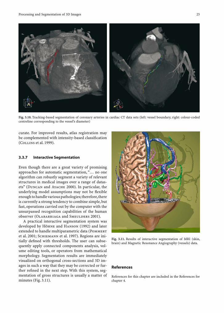
Processing and Segmentation of 3D Images 25

Fig. 3.10. Tracking-based segmentation of coronary arteries in cardiac CT data sets (left: vessel boundary, right: colour-coded centreline corresponding to the vessel’s diameter)

Fig. 3.11. Results of interactive segmentation of MRI (skin, brain) and Magnetic Resonance Angiography (vessels) data.

curate. For improved results, atlas registration may be complemented with intensity-based classifi cation (Collins et al. 1999).

3.3.7 Interactive Segmentation

Even though there are a great variety of promising approaches for automatic segmentation, “… no one algorithm can robustly segment a variety of relevant structures in medical images over a range of datas-ets” (Duncan and Ayache 2000). In particular, the underlying model assumptions may not be fl exible enough to handle various pathologies; therefore, there is currently a strong tendency to combine simple, but fast, operations carried out by the computer with the unsurpassed recognition capabilities of the human observer (Olabarriaga and Smeulders 2001).

A practical interactive segmentation system was developed by Höhne and Hanson (1992) and later extended to handle multiparametric data (Pommert et al. 2001; Schiemann et al. 1997). Regions are ini-tially defi ned with thresholds. The user can subse-quently apply connected components analysis, vol-ume editing tools, or operators from mathematical morphology. Segmentation results are immediately visualized on orthogonal cross-sections and 3D im-ages in such a way that they may be corrected or fur-ther refi ned in the next step. With this system, seg-mentation of gross structures is usually a matter of minutes (Fig. 3.11).

References

References for this chapter are included in the References for chapter 4.

26 G. Sakas and A. Pommert

4 3D Visualization

Georgios Sakas and Andreas Pommert

G. Sakas, PhDFraunhofer Institute for Computer Graphics (IGD), Fraunhoferstr 5, 64283 Darmstadt, GermanyA. Pommert, PhDInstitut für Medizinische Informatik (IMI), Universitätsklinikum Hamburg-Eppendorf, Martinistraße 52, 20246 Hamburg, Germany

4.1 Introduction

After segmentation, the choice of which rendering technique to use must be made. The more traditional surface-based methods fi rst create an intermediate surface representation of the object to be shown. It may then be rendered with any standard computer graphics method. More recently, volume-based meth-ods have been developed which create a 3D view di-rectly from the volume data. These methods use the full gray-level information to render surfaces, cuts, or transparent and semi-transparent volumes. As a third way, transform-based rendering methods may be used.

CONTENTS

4.1 Introduction 264.2 Cut Planes 264.3 Surface Rendering 264.4 Direct Volume Visualization Methods 264.4.1 Scanning the Volume 264.4.2 Splatting in Shear-Warp Space 284.5 Visualization Primitives in Direct Volume Rendering 294.5.1 Maximum and Minimum Intensity Projection 294.5.2 Digitally Reconstructed Radiographies 304.5.3 Direct Surface Rendering 304.5.4 Direct Semi-Transparent Volume Rendering 314.5.5 Volume Rendering Using Transfer Functions 324.6 Transform-Based Rendering 324.7 Image Fusion 344.8 3D Anatomical Atlases 35 References 39

4.2 Cut Planes

Once a surface view is available, a very simple and effective method of visualizing interior structures is cutting. When the original intensity values are mapped onto the cut plane, they can be better un-derstood in their anatomical context (Höhne et al. 1990). A special case is selective cutting, where cer-tain objects are left untouched (Fig. 4.1).

4.3 Surface Rendering

Surface rendering bridges the gap between volume visualization and more traditional computer graph-ics (Foley et al. 1995; Watt 2000). The key idea is to create intermediate surface descriptions of the rel-evant objects from the volume data. Only this infor-mation is then used for rendering images. If triangles are used as surface elements, this process is called triangulation.

An apparent advantage of surface extraction is the potentially very high data reduction from volume to surface representations. Resulting computing times can be further reduced if standard data structures, such as polygon meshes, are used which are supported by standard computer graphics hard- and software.

On the other hand, the extraction step eliminates most of the valuable information on the cross-sec-tional images. Even simple cuts are meaningless be-cause there is no information about the interior of an object, unless the image volume is also available at rendering time. Furthermore, every change of sur-face defi nition criteria, such as adjusting a threshold, requires a recalculation of the whole data structure.

The classic method for surface extraction is the marching-cubes algorithm, developed by Lorensen and Cline (1987). It creates an iso-surface, approxi-mating the location of a certain intensity value in the data volume. This algorithm basically considers cubes

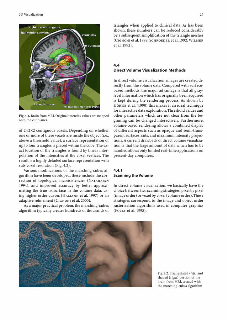
3D Visualization 27

of 2×2×2 contiguous voxels. Depending on whether one or more of these voxels are inside the object (i.e., above a threshold value), a surface representation of up to four triangles is placed within the cube. The ex-act location of the triangles is found by linear inter-polation of the intensities at the voxel vertices. The result is a highly detailed surface representation with sub-voxel resolution (Fig. 4.2).

Various modifi cations of the marching-cubes al-gorithm have been developed; these include the cor-rection of topological inconsistencies (Natarajan 1994), and improved accuracy by better approxi-mating the true isosurface in the volume data, us-ing higher order curves (Hamann et al. 1997) or an adaptive refi nement (Cignoni et al. 2000).

As a major practical problem, the marching-cubes algorithm typically creates hundreds of thousands of

triangles when applied to clinical data. As has been shown, these numbers can be reduced considerably by a subsequent simplifi cation of the triangle meshes (Cignoni et al. 1998; Schroeder et al. 1992; Wilmer et al. 1992).

4.4 Direct Volume Visualization Methods

In direct volume visualization, images are created di-rectly from the volume data. Compared with surface-based methods, the major advantage is that all gray-level information which has originally been acquired is kept during the rendering process. As shown by Höhne et al. (1990) this makes it an ideal technique for interactive data exploration. Threshold values and other parameters which are not clear from the be-ginning can be changed interactively. Furthermore, volume-based rendering allows a combined display of different aspects such as opaque and semi-trans-parent surfaces, cuts, and maximum intensity projec-tions. A current drawback of direct volume visualiza-tion is that the large amount of data which has to be handled allows only limited real-time applications on present-day computers.

4.4.1 Scanning the Volume

In direct volume visualization, we basically have the choice between two scanning strategies: pixel by pixel (image order) or voxel by voxel (volume order). These strategies correspond to the image and object order rasterization algorithms used in computer graphics (Foley et al. 1995).

Fig. 4.1. Brain from MRI. Original intensity values are mapped onto the cut planes.

Fig. 4.2. Triangulated (left) and shaded (right) portion of the brain from MRI, created with the marching-cubes algorithm

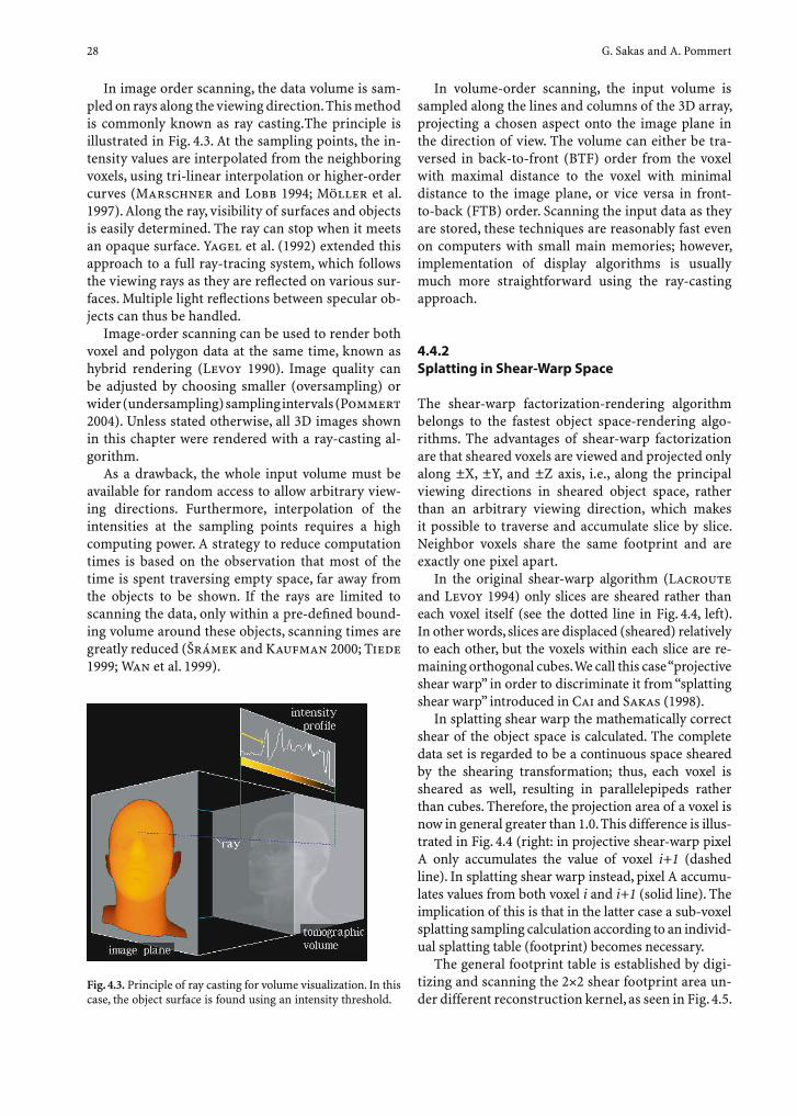
28 G. Sakas and A. Pommert

In image order scanning, the data volume is sam-pled on rays along the viewing direction. This method is commonly known as ray casting.The principle is illustrated in Fig. 4.3. At the sampling points, the in-tensity values are interpolated from the neighboring voxels, using tri-linear interpolation or higher-order curves (Marschner and Lobb 1994; Möller et al. 1997). Along the ray, visibility of surfaces and objects is easily determined. The ray can stop when it meets an opaque surface. Yagel et al. (1992) extended this approach to a full ray-tracing system, which follows the viewing rays as they are refl ected on various sur-faces. Multiple light refl ections between specular ob-jects can thus be handled.

Image-order scanning can be used to render both voxel and polygon data at the same time, known as hybrid rendering (Levoy 1990). Image quality can be adjusted by choosing smaller (oversampling) or wider (undersampling) sampling intervals (Pommert 2004). Unless stated otherwise, all 3D images shown in this chapter were rendered with a ray-casting al-gorithm.

As a drawback, the whole input volume must be available for random access to allow arbitrary view-ing directions. Furthermore, interpolation of the intensities at the sampling points requires a high computing power. A strategy to reduce computation times is based on the observation that most of the time is spent traversing empty space, far away from the objects to be shown. If the rays are limited to scanning the data, only within a pre-defi ned bound-ing volume around these objects, scanning times are greatly reduced (Šrámek and Kaufman 2000; Tiede 1999; Wan et al. 1999).

In volume-order scanning, the input volume is sampled along the lines and columns of the 3D array, projecting a chosen aspect onto the image plane in the direction of view. The volume can either be tra-versed in back-to-front (BTF) order from the voxel with maximal distance to the voxel with minimal distance to the image plane, or vice versa in front-to-back (FTB) order. Scanning the input data as they are stored, these techniques are reasonably fast even on computers with small main memories; however, implementation of display algorithms is usually much more straightforward using the ray-casting approach.

4.4.2 Splatting in Shear-Warp Space

The shear-warp factorization-rendering algorithm belongs to the fastest object space-rendering algo-rithms. The advantages of shear-warp factorization are that sheared voxels are viewed and projected only along ±X, ±Y, and ±Z axis, i.e., along the principal viewing directions in sheared object space, rather than an arbitrary viewing direction, which makes it possible to traverse and accumulate slice by slice. Neighbor voxels share the same footprint and are exactly one pixel apart.

In the original shear-warp algorithm (Lacroute and Levoy 1994) only slices are sheared rather than each voxel itself (see the dotted line in Fig. 4.4, left). In other words, slices are displaced (sheared) relatively to each other, but the voxels within each slice are re-maining orthogonal cubes. We call this case “projective shear warp” in order to discriminate it from “splatting shear warp” introduced in Cai and Sakas (1998).

In splatting shear warp the mathematically correct shear of the object space is calculated. The complete data set is regarded to be a continuous space sheared by the shearing transformation; thus, each voxel is sheared as well, resulting in parallelepipeds rather than cubes. Therefore, the projection area of a voxel is now in general greater than 1.0. This difference is illus-trated in Fig. 4.4 (right: in projective shear-warp pixel A only accumulates the value of voxel i+1 (dashed line). In splatting shear warp instead, pixel A accumu-lates values from both voxel i and i+1 (solid line). The implication of this is that in the latter case a sub-voxel splatting sampling calculation according to an individ-ual splatting table (footprint) becomes necessary.

The general footprint table is established by digi-tizing and scanning the 2×2 shear footprint area un-der different reconstruction kernel, as seen in Fig. 4.5.

Fig. 4.3. Principle of ray casting for volume visualization. In this case, the object surface is found using an intensity threshold.

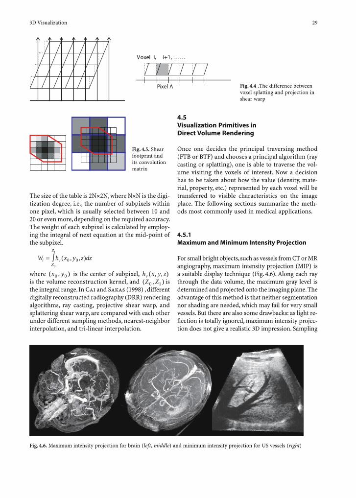
3D Visualization 29

The size of the table is 2N×2N, where N×N is the digi-tization degree, i.e., the number of subpixels within one pixel, which is usually selected between 10 and 20 or even more, depending on the required accuracy. The weight of each subpixel is calculated by employ-ing the integral of next equation at the mid-point of the subpixel.

W h x y z dzi vZ

Z

= ∫ ( , , )0 00

1

where ( , )x y0 0 is the center of subpixel, h x y zv ( , , ) is the volume reconstruction kernel, and ( , )Z Z0 1 is the integral range. In Cai and Sakas (1998) , different digitally reconstructed radiography (DRR) rendering algorithms, ray casting, projective shear warp, and splattering shear warp, are compared with each other under different sampling methods, nearest-neighbor interpolation, and tri-linear interpolation.

4.5 Visualization Primitives in Direct Volume Rendering

Once one decides the principal traversing method (FTB or BTF) and chooses a principal algorithm (ray casting or splatting), one is able to traverse the vol-ume visiting the voxels of interest. Now a decision has to be taken about how the value (density, mate-rial, property, etc.) represented by each voxel will be transferred to visible characteristics on the image place. The following sections summarize the meth-ods most commonly used in medical applications.

4.5.1 Maximum and Minimum Intensity Projection

For small bright objects, such as vessels from CT or MR angiography, maximum intensity projection (MIP) is a suitable display technique (Fig. 4.6). Along each ray through the data volume, the maximum gray level is determined and projected onto the imaging plane. The advantage of this method is that neither segmentation nor shading are needed, which may fail for very small vessels. But there are also some drawbacks: as light re-fl ection is totally ignored, maximum intensity projec-tion does not give a realistic 3D impression. Sampling

Fig. 4.4 .The difference between voxel splatting and projection in shear warp

Fig. 4.5. Shear footprint and its convolution matrix

Fig. 4.6. Maximum intensity projection for brain (left, middle) and minimum intensity projection for US vessels (right)

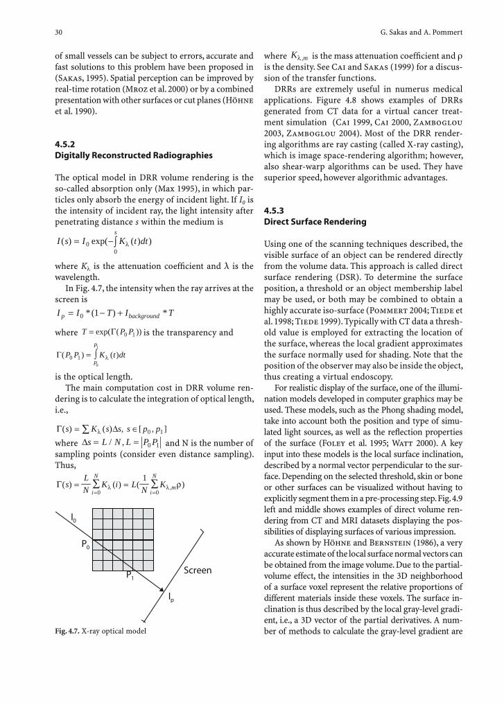
30 G. Sakas and A. Pommert

of small vessels can be subject to errors, accurate and fast solutions to this problem have been proposed in (Sakas, 1995). Spatial perception can be improved by real-time rotation (Mroz et al. 2000) or by a combined presentation with other surfaces or cut planes (Höhne et al. 1990).

4.5.2 Digitally Reconstructed Radiographies

The optical model in DRR volume rendering is the so-called absorption only (Max 1995), in which par-ticles only absorb the energy of incident light. If I0 is the intensity of incident ray, the light intensity after penetrating distance s within the medium is

I s I K t dts

( ) exp( ( ) )= −∫00

λ

where K is the attenuation coeffi cient and l is the wavelength.

In Fig. 4.7, the intensity when the ray arrives at the screen is

I I T I Tp background= − +0 1*( ) *

where T P P= exp( ( ))Γ 0 1 is the transparency and

Γ( ) ( )P P K t dtP

P

0 10

1

= ∫ λ

is the optical length.The main computation cost in DRR volume ren-

dering is to calculate the integration of optical length, i.e.,

Γ ∆( ) ( ) , [ , ]s K s s s p p= ∈∑ λ 0 1

where ∆s L N L P P= =/ , 0 1 and N is the number of

sampling points (consider even distance sampling). Thus,

Γ( ) ( ) ( ),sL

NK i L

NK

i

N

mi

N

= == =∑ ∑λ λ ρ

0 0

1

where K mλ , is the mass attenuation coeffi cient and

is the density. See Cai and Sakas (1999) for a discus-sion of the transfer functions.

DRRs are extremely useful in numerus medical applications. Figure 4.8 shows examples of DRRs generated from CT data for a virtual cancer treat-ment simulation (Cai 1999, Cai 2000, Zamboglou 2003, Zamboglou 2004). Most of the DRR render-ing algorithms are ray casting (called X-ray casting), which is image space-rendering algorithm; however, also shear-warp algorithms can be used. They have superior speed, however algorithmic advantages.

4.5.3 Direct Surface Rendering

Using one of the scanning techniques described, the visible surface of an object can be rendered directly from the volume data. This approach is called direct surface rendering (DSR). To determine the surface position, a threshold or an object membership label may be used, or both may be combined to obtain a highly accurate iso-surface (Pommert 2004; Tiede et al. 1998; Tiede 1999). Typically with CT data a thresh-old value is employed for extracting the location of the surface, whereas the local gradient approximates the surface normally used for shading. Note that the position of the observer may also be inside the object, thus creating a virtual endoscopy.

For realistic display of the surface, one of the illumi-nation models developed in computer graphics may be used. These models, such as the Phong shading model, take into account both the position and type of simu-lated light sources, as well as the refl ection properties of the surface (Foley et al. 1995; Watt 2000). A key input into these models is the local surface inclination, described by a normal vector perpendicular to the sur-face. Depending on the selected threshold, skin or bone or other surfaces can be visualized without having to explicitly segment them in a pre-processing step. Fig. 4.9 left and middle shows examples of direct volume ren-dering from CT and MRI datasets displaying the pos-sibilities of displaying surfaces of various impression.

As shown by Höhne and Bernstein (1986), a very accurate estimate of the local surface normal vectors can be obtained from the image volume. Due to the partial-volume effect, the intensities in the 3D neighborhood of a surface voxel represent the relative proportions of different materials inside these voxels. The surface in-clination is thus described by the local gray-level gradi-ent, i.e., a 3D vector of the partial derivatives. A num-ber of methods to calculate the gray-level gradient are Fig. 4.7. X-ray optical model

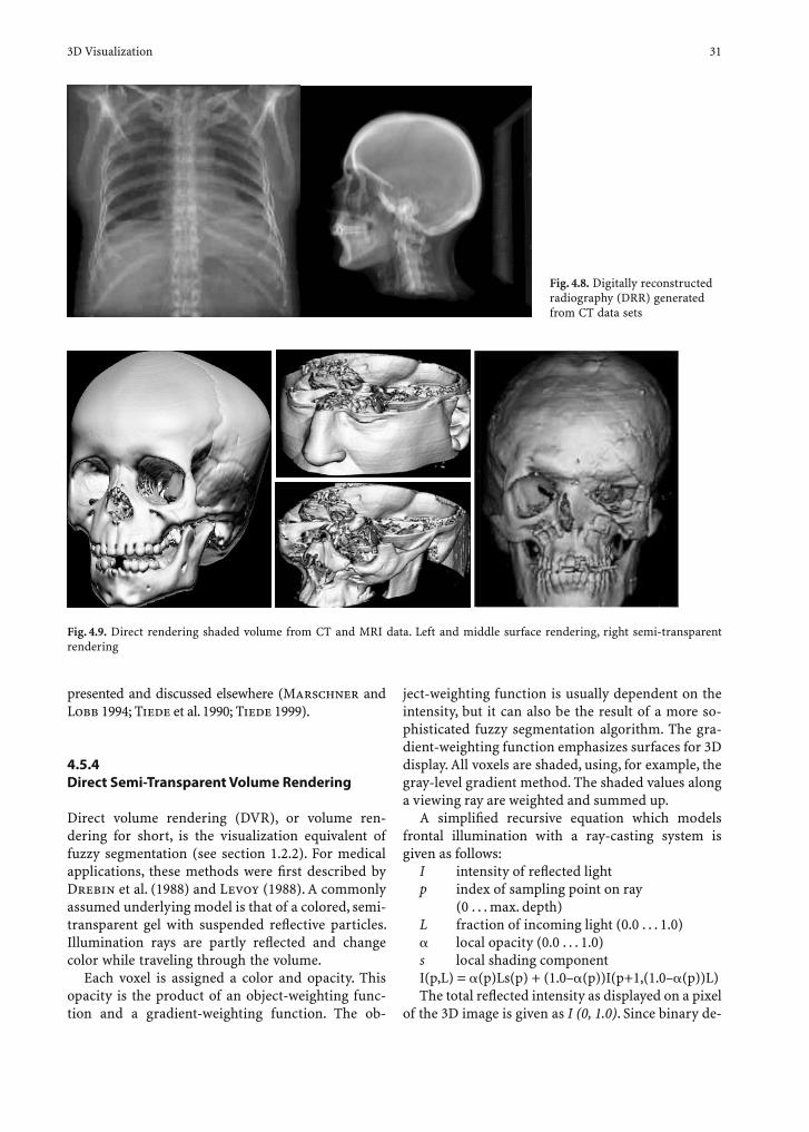
3D Visualization 31

presented and discussed elsewhere (Marschner and Lobb 1994; Tiede et al. 1990; Tiede 1999).

4.5.4 Direct Semi-Transparent Volume Rendering

Direct volume rendering (DVR), or volume ren-dering for short, is the visualization equivalent of fuzzy segmentation (see section 1.2.2). For medical applications, these methods were fi rst described by Drebin et al. (1988) and Levoy (1988). A commonly assumed underlying model is that of a colored, semi-transparent gel with suspended refl ective particles. Illumination rays are partly refl ected and change color while traveling through the volume.

Each voxel is assigned a color and opacity. This opacity is the product of an object-weighting func-tion and a gradient-weighting function. The ob-

ject-weighting function is usually dependent on the intensity, but it can also be the result of a more so-phisticated fuzzy segmentation algorithm. The gra-dient-weighting function emphasizes surfaces for 3D display. All voxels are shaded, using, for example, the gray-level gradient method. The shaded values along a viewing ray are weighted and summed up.

A simplifi ed recursive equation which models frontal illumination with a ray-casting system is given as follows:

I intensity of refl ected lightp index of sampling point on ray (0 . . . max. depth)L fraction of incoming light (0.0 . . . 1.0)� local opacity (0.0 . . . 1.0)s local shading componentI(p,L) = �(p)Ls(p) + (1.0–�(p))I(p+1,(1.0–�(p))L)The total refl ected intensity as displayed on a pixel

of the 3D image is given as I (0, 1.0). Since binary de-

Fig. 4.8. Digitally reconstructed radiography (DRR) generated from CT data sets

Fig. 4.9. Direct rendering shaded volume from CT and MRI data. Left and middle surface rendering, right semi-transparent rendering

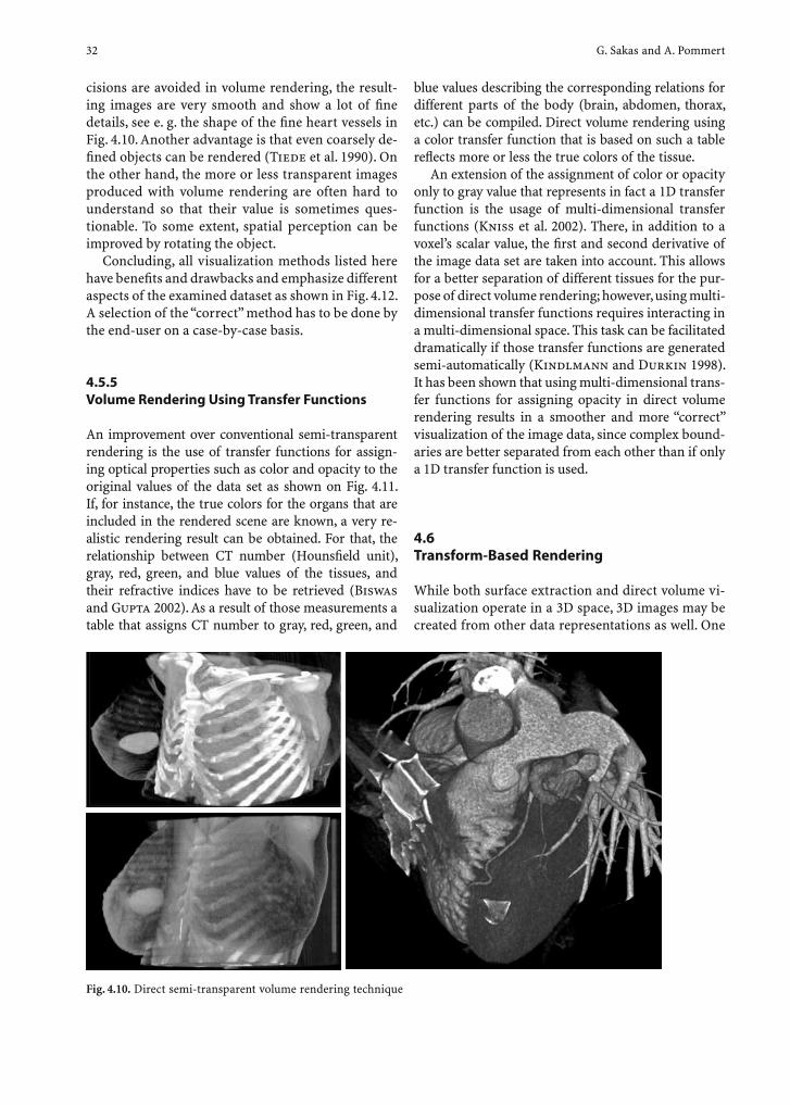
32 G. Sakas and A. Pommert

cisions are avoided in volume rendering, the result-ing images are very smooth and show a lot of fi ne details, see e. g. the shape of the fi ne heart vessels in Fig. 4.10. Another advantage is that even coarsely de-fi ned objects can be rendered (Tiede et al. 1990). On the other hand, the more or less transparent images produced with volume rendering are often hard to understand so that their value is sometimes ques-tionable. To some extent, spatial perception can be improved by rotating the object.

Concluding, all visualization methods listed here have benefi ts and drawbacks and emphasize different aspects of the examined dataset as shown in Fig. 4.12. A selection of the “correct” method has to be done by the end-user on a case-by-case basis.

4.5.5 Volume Rendering Using Transfer Functions

An improvement over conventional semi-transparent rendering is the use of transfer functions for assign-ing optical properties such as color and opacity to the original values of the data set as shown on Fig. 4.11. If, for instance, the true colors for the organs that are included in the rendered scene are known, a very re-alistic rendering result can be obtained. For that, the relationship between CT number (Hounsfi eld unit), gray, red, green, and blue values of the tissues, and their refractive indices have to be retrieved (Biswas and Gupta 2002). As a result of those measurements a table that assigns CT number to gray, red, green, and

blue values describing the corresponding relations for different parts of the body (brain, abdomen, thorax, etc.) can be compiled. Direct volume rendering using a color transfer function that is based on such a table refl ects more or less the true colors of the tissue.

An extension of the assignment of color or opacity only to gray value that represents in fact a 1D transfer function is the usage of multi-dimensional transfer functions (Kniss et al. 2002). There, in addition to a voxel’s scalar value, the fi rst and second derivative of the image data set are taken into account. This allows for a better separation of different tissues for the pur-pose of direct volume rendering; however, using multi-dimensional transfer functions requires interacting in a multi-dimensional space. This task can be facilitated dramatically if those transfer functions are generated semi-automatically (Kindlmann and Durkin 1998). It has been shown that using multi-dimensional trans-fer functions for assigning opacity in direct volume rendering results in a smoother and more “correct” visualization of the image data, since complex bound-aries are better separated from each other than if only a 1D transfer function is used.

4.6 Transform-Based Rendering

While both surface extraction and direct volume vi-sualization operate in a 3D space, 3D images may be created from other data representations as well. One

Fig. 4.10. Direct semi-transparent volume rendering technique

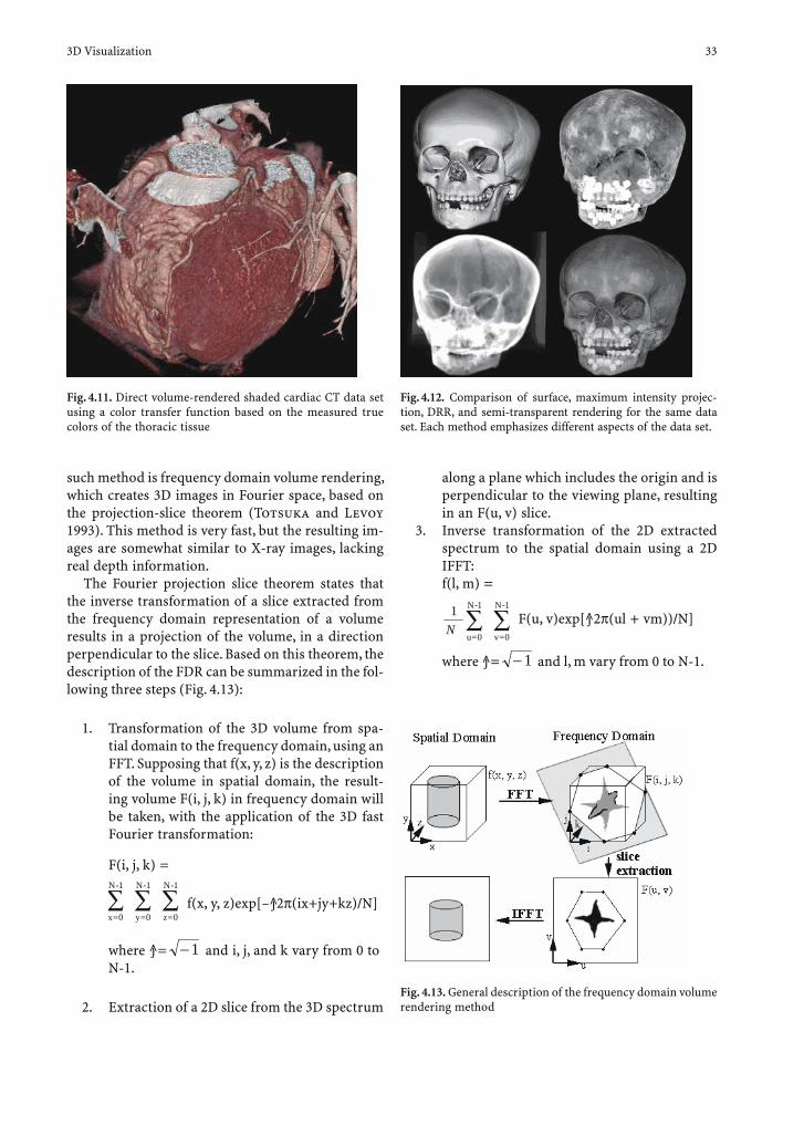
3D Visualization 33

such method is frequency domain volume rendering, which creates 3D images in Fourier space, based on the projection-slice theorem (Totsuka and Levoy 1993). This method is very fast, but the resulting im-ages are somewhat similar to X-ray images, lacking real depth information.

The Fourier projection slice theorem states that the inverse transformation of a slice extracted from the frequency domain representation of a volume results in a projection of the volume, in a direction perpendicular to the slice. Based on this theorem, the description of the FDR can be summarized in the fol-lowing three steps (Fig. 4.13):

1. Transformation of the 3D volume from spa-tial domain to the frequency domain, using an FFT. Supposing that f(x, y, z) is the description of the volume in spatial domain, the result-ing volume F(i, j, k) in frequency domain will be taken, with the application of the 3D fast Fourier transformation:

F(i, j, k) =

x=0

N-1

∑y=0

N-1

∑z=0

N-1

∑ f(x, y, z)exp[– j 2π(ix+jy+kz)/N]

where j = −1 and i, j, and k vary from 0 to

N-1.

2. Extraction of a 2D slice from the 3D spectrum

along a plane which includes the origin and is perpendicular to the viewing plane, resulting in an F(u, v) slice.

3. Inverse transformation of the 2D extracted spectrum to the spatial domain using a 2D IFFT:f(l, m) =

1N

u=0

N-1

∑v=0

N-1

∑ F(u, v)exp[ j 2π(ul + vm))/N]

where j = −1 and l, m vary from 0 to N-1.

Fig. 4.11. Direct volume-rendered shaded cardiac CT data set using a color transfer function based on the measured true colors of the thoracic tissue

Fig. 4.12. Comparison of surface, maximum intensity projec-tion, DRR, and semi-transparent rendering for the same data set. Each method emphasizes different aspects of the data set.

Fig. 4.13. General description of the frequency domain volume rendering method

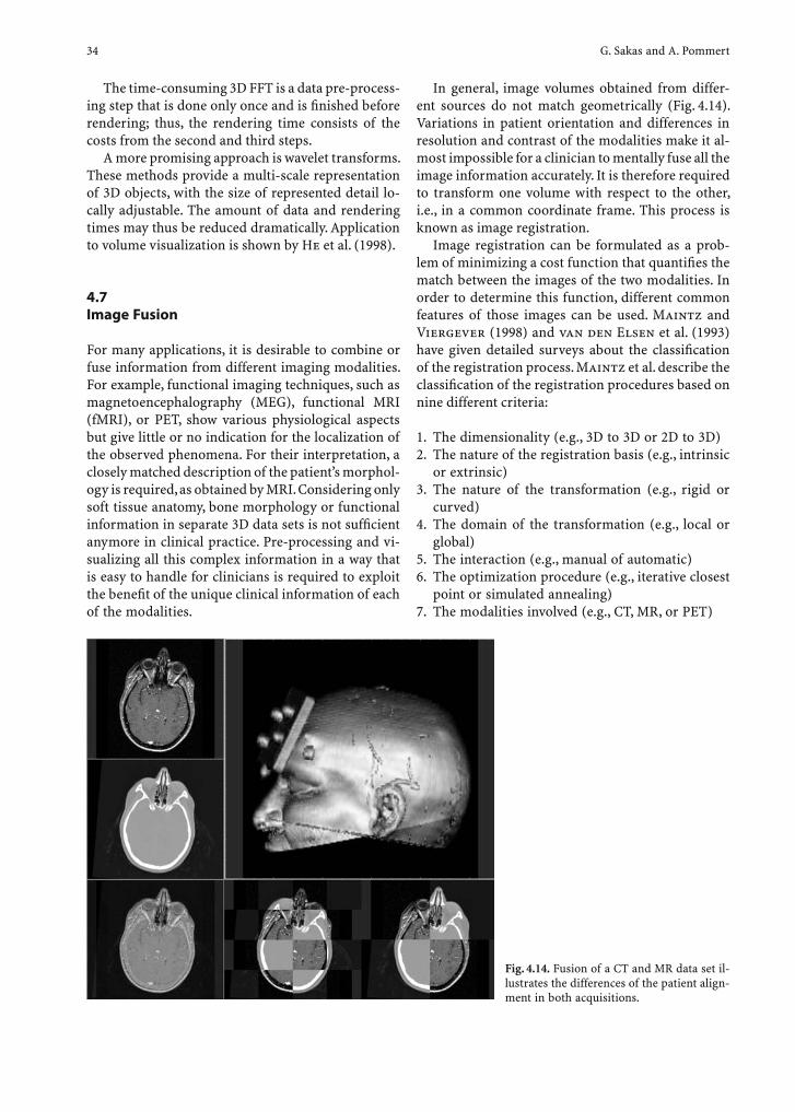
34 G. Sakas and A. Pommert

The time-consuming 3D FFT is a data pre-process-ing step that is done only once and is fi nished before rendering; thus, the rendering time consists of the costs from the second and third steps.

A more promising approach is wavelet transforms. These methods provide a multi-scale representation of 3D objects, with the size of represented detail lo-cally adjustable. The amount of data and rendering times may thus be reduced dramatically. Application to volume visualization is shown by He et al. (1998).

4.7 Image Fusion

For many applications, it is desirable to combine or fuse information from different imaging modalities. For example, functional imaging techniques, such as magnetoencephalography (MEG), functional MRI (fMRI), or PET, show various physiological aspects but give little or no indication for the localization of the observed phenomena. For their interpretation, a closely matched description of the patient’s morphol-ogy is required, as obtained by MRI. Considering only soft tissue anatomy, bone morphology or functional information in separate 3D data sets is not suffi cient anymore in clinical practice. Pre-processing and vi-sualizing all this complex information in a way that is easy to handle for clinicians is required to exploit the benefi t of the unique clinical information of each of the modalities.

In general, image volumes obtained from differ-ent sources do not match geometrically (Fig. 4.14). Variations in patient orientation and differences in resolution and contrast of the modalities make it al-most impossible for a clinician to mentally fuse all the image information accurately. It is therefore required to transform one volume with respect to the other, i.e., in a common coordinate frame. This process is known as image registration.

Image registration can be formulated as a prob-lem of minimizing a cost function that quantifi es the match between the images of the two modalities. In order to determine this function, different common features of those images can be used. Maintz and Viergever (1998) and van den Elsen et al. (1993) have given detailed surveys about the classifi cation of the registration process. Maintz et al. describe the classifi cation of the registration procedures based on nine different criteria:

1. The dimensionality (e.g., 3D to 3D or 2D to 3D)2. The nature of the registration basis (e.g., intrinsic

or extrinsic)3. The nature of the transformation (e.g., rigid or

curved)4. The domain of the transformation (e.g., local or

global)5. The interaction (e.g., manual of automatic)6. The optimization procedure (e.g., iterative closest

point or simulated annealing)7. The modalities involved (e.g., CT, MR, or PET)

Fig. 4.14. Fusion of a CT and MR data set il-lustrates the differences of the patient align-ment in both acquisitions.

3D Visualization 35

Fig. 4.15. Fusion of different imaging modalities for therapy control in a clinical study of obsessive-compulsive disorder. Magnetic resonance imaging shows that morphology is com-bined with a positron emission tomography (PET) scan, which shows glucose metabolism. Since the entire volume is mapped, the activity can be explored at any location of the brain.

8. The subject (e.g., inter-subject, intra-subject, or atlas)

9. The object (e.g., head or abdomen)

When considering the nature of the registration base, for example, the transformation may be defi ned using corresponding landmarks in both data sets. In a simple case, artifi cial markers attached to the patient are available which are visible on different modalities (Bromm and Scharein 1996); otherwise, pairs of preferably stable matching points, such as the AC–PC line, may be used. A more robust approach is to interactively match larger features such as surfaces (Schiemann et al. 1994). Figure 4.15 shows the result of the registration of a PET and an MRI data set.

Segmentation-based registration approaches canbe divided into those using rigid models, such as, points, curves, or surfaces, and those using deformable models (e.g., snakes or nets). In all cases the registra-tion accuracy of this method is limited to the accuracy of the segmentation step. Herewith any two modalities can be registered given the fact that the structures are visible within both. As an example, in some cases the target area in US images is not as visible as it should be to ensure a qualitatively high treatment of prostate cancer, whereas other modalities, such as CT, provide a better image. Unfortunately, CT cannot be used in a live-imaging procedure in the treatment room during intervention such as ultrasound imaging. To overcome these limitations, the images of both modalities can be registered in a unique data set, i.e., gathering pre-operatively a CT volume and using it in combination with the intra-operative US-guided live procedure. To realize this, the separate volumes of CT and US can be registered with respect to each other based on the ge-ometry of the urethra or by mutual information based on their greylevels as shown in Fig. 4.16 (Firle et al. 2003).

In a fundamentally different approach, the results of a registration step are evaluated at every point of the combined volume, based on intensity values (Studholme et al. 1996; Wells et al. 1996). Starting from a coarse match, registration is achieved by adjust-ing position and orientation until the mutual informa-tion (“similarity”) between both data sets is maximized. These methods are fully automatic, do not rely on a possibly erroneous defi nition of landmarks, and seem to be more accurate than others (West et al. 1997).

Mutual information, originating in the information theory, is a voxel-based similarity measure of the sta-tistical dependency between two data sets, which has been proposed by Collignon et al. (1995) and Viola and Wells (1997). It evaluates the amount of infor-

mation that one variable contains about the other. By superimposing two data sets of the same object, but from different modalities, this method states that they are correctly aligned if the mutual information of geometrically corresponding gray values is maximal. Since no assumptions are made about the two signals, this method is not restricted to specifi c modalities and does not require the extraction of features in a pre-processing step. A recent survey about mutual infor-mation-based registration approaches was given by Pluim et al. (2003; Figs. 4.17, 4.18).

The calculation of the transformation based on mutual information is a very time-consuming opti-mization process. Exploiting the coarse-to-fi ne reso-lution strategy (pyramidal approach) is one com-mon possibility to speed up the registration process (Pluim et al. 2001). Another approach, when allow-ing only rigid transformations, is the usage of the “3D cross model” (Firle et al. 2004). This partial-volume based matching assumes that the center of the vol-ume comprises the majority of the overlapping infor-mation between both images. The data from all three directions through the reference image (Maes et al. 1997) is taken without any high sub-sampling factors or lowering the number of histogram bins (Capek et al. 2001). Figures 4.17 and 4.18 depict the registration result of a whole-body CT and PET data set.

4.8 3D Anatomical Atlases

Whereas in classical medicine knowledge about the human body is represented in books and atlases,

36 G. Sakas and A. Pommert

Fig. 4.16. Fusion of CT and 3D US volumes based on the urethra geometry (upper) and MRI with 3D U/S based on mutual information (lower)

Fig. 4.17. While CT identifi es the precise size, shape, and loca-tion of a mass, PET detects changes in the metabolism caused by the growth of abnormal cells in it. Fusion of the whole-body scans of both modalities

Fig. 4.18. A 3D image fusion after mutual-information-based registration of a CT and PET data set. Blending of the PET into the CT volume using image-level intermixing and differ-ent opacity settings

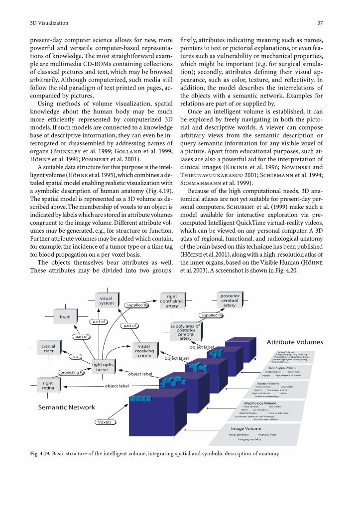
3D Visualization 37

present-day computer science allows for new, more powerful and versatile computer-based representa-tions of knowledge. The most straightforward exam-ple are multimedia CD-ROMs containing collections of classical pictures and text, which may be browsed arbitrarily. Although computerized, such media still follow the old paradigm of text printed on pages, ac-companied by pictures.

Using methods of volume visualization, spatial knowledge about the human body may be much more effi ciently represented by computerized 3D models. If such models are connected to a knowledge base of descriptive information, they can even be in-terrogated or disassembled by addressing names of organs (Brinkley et al. 1999; Golland et al. 1999; Höhne et al. 1996; Pommert et al. 2001).

A suitable data structure for this purpose is the intel-ligent volume (Höhne et al. 1995), which combines a de-tailed spatial model enabling realistic visualization with a symbolic description of human anatomy (Fig. 4.19). The spatial model is represented as a 3D volume as de-scribed above. The membership of voxels to an object is indicated by labels which are stored in attribute volumes congruent to the image volume. Different attribute vol-umes may be generated, e.g., for structure or function. Further attribute volumes may be added which contain, for example, the incidence of a tumor type or a time tag for blood propagation on a per-voxel basis.

The objects themselves bear attributes as well. These attributes may be divided into two groups:

fi rstly, attributes indicating meaning such as names, pointers to text or pictorial explanations, or even fea-tures such as vulnerability or mechanical properties, which might be important (e.g. for surgical simula-tion); secondly, attributes defi ning their visual ap-pearance, such as color, texture, and refl ectivity. In addition, the model describes the interrelations of the objects with a semantic network. Examples for relations are part of or supplied by.

Once an intelligent volume is established, it can be explored by freely navigating in both the picto-rial and descriptive worlds. A viewer can compose arbitrary views from the semantic description or query semantic information for any visible voxel of a picture. Apart from educational purposes, such at-lases are also a powerful aid for the interpretation of clinical images (Kikinis et al. 1996; Nowinski and Thirunavuukarasuu 2001; Schiemann et al. 1994; Schmahmann et al. 1999).

Because of the high computational needs, 3D ana-tomical atlases are not yet suitable for present-day per-sonal computers. Schubert et al. (1999) make such a model available for interactive exploration via pre-computed Intelligent QuickTime virtual-reality videos, which can be viewed on any personal computer. A 3D atlas of regional, functional, and radiological anatomy of the brain based on this technique has been published (Höhne et al. 2001), along with a high-resolution atlas of the inner organs, based on the Visible Human (Höhne et al. 2003). A screenshot is shown in Fig. 4.20.

Fig. 4.19. Basic structure of the intelligent volume, integrating spatial and symbolic description of anatomy

38 G. Sakas and A. Pommert

To date, most 3D anatomical atlases are based on the data derived from one individual only. The inter-individual variability of organ shape and topology in space and time is thus not yet part of the model. Methods for measuring and modeling variability are currently being developed (Mazziotta et al. 1995; Styner and Gerig 2001; Thompson et al. 2000).

AcknowledgementsWe thank C. Dold, E. Firle, K.-H. Höhne, G. Karangelis, T. Schiemann, U. Tiede, and S. Wesarg for their con-tributions to this work.

References

Arata LK, Dhawan AP, Broderick JP, Gaskil-Shipley MF, Levy AV, Volkow ND (1995) Three-dimensional anatomical model-based segmentation of MR brain images through principal axes registration. IEEE Trans Biomed Eng 42:1069–1078

Arnold JB, Liow J-S, Schaper KA, Stern JJ, Sled JG, Shattuck DW, Worth AJ, Cohen MS, Leahy RM, Mazziotta JC, Rottenberg DA (2001) Qualitative and quantitative evaluation of six algo-rithms for correcting intensity nonuniformity effects. Neuro-Image 13:931–943

Biswas TK, Gupta AK (2002). Retrieval of true color of the inter-nal organ of CT images and attempt to tissue characterization by refractive index: initial experience. Ind J Radiol Imaging 12:169–178

Bomans M, Riemer M, Tiede U, Höhne KH (1987) 3D-Segmenta-tion von Kernspin-Tomogrammen. In: Paulus E (ed) Muster-

Fig. 4.20. User interface of VOXEL-MAN 3D-Navigator: brain and skull, a PC-based 3D atlas of regional, functional, and radio-logical anatomy. The user may navigate freely in both the pictorial (left) and descriptive (right) context.

erkennung 1987. Proc of the 9th DAGM symposium. Infor-matik-Fachberichte, vol 149. Springer, Berlin Heidelberg New York, pp 231–235

Brinkley JF, Wong BA, Hinshaw KP, Rosse C (1999) Design of an anatomy information system. IEEE Comput Graphics Appl 19:38–48

Bromm B, Scharein E (1996) Visualisation of pain by magne-toencephalography in humans. In: Höhne KH, Kikinis R (eds) Visualization in biomedical computing. Proc VBC ‘96. Springer, Berlin Heidelberg New York, pp 477–481 (Lect Notes Comput Sci, vol 1131)

Cai W, Sakas G (1998) Maximum intensity projection using splat-ting in sheared object space. Comput Graph Forum 17:113–124

Cai W, Sakas G, (1999) Transfer functions in DRR volume ren-dering. In: Lemke HU et al. Computer assisted radiology and surgery (CARS). Proceedings. Amsterdam, Lausanne:Elsevier, pp. 284–289 (International Congress Series 1191).

Cai W, Karangelis G, Sakas G (1999)Volume interaction techniques in the virtual simulation of radiotherapy treatment planning. In: Keldysh Institute of Applied Mathematics: Graphicon. Pro-ceedings. Moscow, pp. 231–239

Cai W, Walter S, Karangelis G, Sakas G (2000) Collaborative virtual simulation environment for radiotherapy treatment planning. In: Computer Graphics Forum 19, 3 pp. C-379 –C-390

Canny J (1986) A computational approach to edge detection. IEEE Trans Pattern Anal Machine Intell 8:679–698

Capek M, Mroz L, Wegenkittl R (2001) Robust and fast medical registration of 3D multi-modality data sets, Medicon 2001, IXth Mediterranean conference on medical and biological engineering and computing, Pula, Croatia, pp 515–518

Caselles V, Kimmel R, Sapiro G (1997). Geodesic active contours. International Journal on Computer Vision, 22(1):61–97, 1997

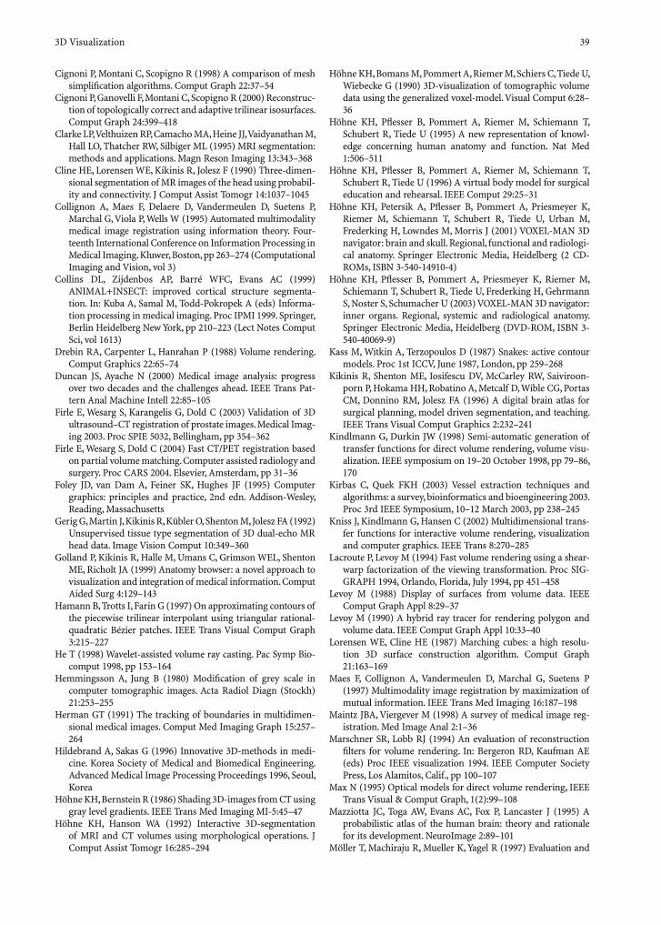
3D Visualization 39

Cignoni P, Montani C, Scopigno R (1998) A comparison of mesh simplifi cation algorithms. Comput Graph 22:37–54

Cignoni P, Ganovelli F, Montani C, Scopigno R (2000) Reconstruc-tion of topologically correct and adaptive trilinear isosurfaces. Comput Graph 24:399–418

Clarke LP, Velthuizen RP, Camacho MA, Heine JJ, Vaidyanathan M, Hall LO, Thatcher RW, Silbiger ML (1995) MRI segmentation: methods and applications. Magn Reson Imaging 13:343–368

Cline HE, Lorensen WE, Kikinis R, Jolesz F (1990) Three-dimen-sional segmentation of MR images of the head using probabil-ity and connectivity. J Comput Assist Tomogr 14:1037–1045

Collignon A, Maes F, Delaere D, Vandermeulen D, Suetens P, Marchal G, Viola P, Wells W (1995) Automated multimodality medical image registration using information theory. Four-teenth International Conference on Information Processing in Medical Imaging. Kluwer, Boston, pp 263–274 (Computational Imaging and Vision, vol 3)

Collins DL, Zijdenbos AP, Barré WFC, Evans AC (1999) ANIMAL+INSECT: improved cortical structure segmenta-tion. In: Kuba A, Samal M, Todd-Pokropek A (eds) Informa-tion processing in medical imaging. Proc IPMI 1999. Springer, Berlin Heidelberg New York, pp 210–223 (Lect Notes Comput Sci, vol 1613)

Drebin RA, Carpenter L, Hanrahan P (1988) Volume rendering. Comput Graphics 22:65–74

Duncan JS, Ayache N (2000) Medical image analysis: progress over two decades and the challenges ahead. IEEE Trans Pat-tern Anal Machine Intell 22:85–105

Firle E, Wesarg S, Karangelis G, Dold C (2003) Validation of 3D ultrasound–CT registration of prostate images. Medical Imag-ing 2003. Proc SPIE 5032, Bellingham, pp 354–362

Firle E, Wesarg S, Dold C (2004) Fast CT/PET registration based on partial volume matching. Computer assisted radiology and surgery. Proc CARS 2004. Elsevier, Amsterdam, pp 31–36

Foley JD, van Dam A, Feiner SK, Hughes JF (1995) Computer graphics: principles and practice, 2nd edn. Addison-Wesley, Reading, Massachusetts

Gerig G, Martin J, Kikinis R, Kübler O, Shenton M, Jolesz FA (1992) Unsupervised tissue type segmentation of 3D dual-echo MR head data. Image Vision Comput 10:349–360

Golland P, Kikinis R, Halle M, Umans C, Grimson WEL, Shenton ME, Richolt JA (1999) Anatomy browser: a novel approach to visualization and integration of medical information. Comput Aided Surg 4:129–143

Hamann B, Trotts I, Farin G (1997) On approximating contours of the piecewise trilinear interpolant using triangular rational-quadratic Bézier patches. IEEE Trans Visual Comput Graph 3:215–227

He T (1998) Wavelet-assisted volume ray casting. Pac Symp Bio-comput 1998, pp 153–164

Hemmingsson A, Jung B (1980) Modifi cation of grey scale in computer tomographic images. Acta Radiol Diagn (Stockh) 21:253–255

Herman GT (1991) The tracking of boundaries in multidimen-sional medical images. Comput Med Imaging Graph 15:257–264

Hildebrand A, Sakas G (1996) Innovative 3D-methods in medi-cine. Korea Society of Medical and Biomedical Engineering. Advanced Medical Image Processing Proceedings 1996, Seoul, Korea

Höhne KH, Bernstein R (1986) Shading 3D-images from CT using gray level gradients. IEEE Trans Med Imaging MI-5:45–47

Höhne KH, Hanson WA (1992) Interactive 3D-segmentation of MRI and CT volumes using morphological operations. J Comput Assist Tomogr 16:285–294

Höhne KH, Bomans M, Pommert A, Riemer M, Schiers C, Tiede U, Wiebecke G (1990) 3D-visualization of tomographic volume data using the generalized voxel-model. Visual Comput 6:28–36

Höhne KH, Pfl esser B, Pommert A, Riemer M, Schiemann T, Schubert R, Tiede U (1995) A new representation of knowl-edge concerning human anatomy and function. Nat Med 1:506–511

Höhne KH, Pfl esser B, Pommert A, Riemer M, Schiemann T, Schubert R, Tiede U (1996) A virtual body model for surgical education and rehearsal. IEEE Comput 29:25–31

Höhne KH, Petersik A, Pfl esser B, Pommert A, Priesmeyer K, Riemer M, Schiemann T, Schubert R, Tiede U, Urban M, Frederking H, Lowndes M, Morris J (2001) VOXEL-MAN 3D navigator: brain and skull. Regional, functional and radiologi-cal anatomy. Springer Electronic Media, Heidelberg (2 CD-ROMs, ISBN 3-540-14910-4)

Höhne KH, Pfl esser B, Pommert A, Priesmeyer K, Riemer M, Schiemann T, Schubert R, Tiede U, Frederking H, Gehrmann S, Noster S, Schumacher U (2003) VOXEL-MAN 3D navigator: inner organs. Regional, systemic and radiological anatomy. Springer Electronic Media, Heidelberg (DVD-ROM, ISBN 3-540-40069-9)

Kass M, Witkin A, Terzopoulos D (1987) Snakes: active contour models. Proc 1st ICCV, June 1987, London, pp 259–268

Kikinis R, Shenton ME, Iosifescu DV, McCarley RW, Saiviroon-porn P, Hokama HH, Robatino A, Metcalf D, Wible CG, Portas CM, Donnino RM, Jolesz FA (1996) A digital brain atlas for surgical planning, model driven segmentation, and teaching. IEEE Trans Visual Comput Graphics 2:232–241

Kindlmann G, Durkin JW (1998) Semi-automatic generation of transfer functions for direct volume rendering, volume visu-alization. IEEE symposium on 19–20 October 1998, pp 79–86, 170

Kirbas C, Quek FKH (2003) Vessel extraction techniques and algorithms: a survey, bioinformatics and bioengineering 2003. Proc 3rd IEEE Symposium, 10–12 March 2003, pp 238–245

Kniss J, Kindlmann G, Hansen C (2002) Multidimensional trans-fer functions for interactive volume rendering, visualization and computer graphics. IEEE Trans 8:270–285

Lacroute P, Levoy M (1994) Fast volume rendering using a shear-warp factorization of the viewing transformation. Proc SIG-GRAPH 1994, Orlando, Florida, July 1994, pp 451–458

Levoy M (1988) Display of surfaces from volume data. IEEE Comput Graph Appl 8:29–37

Levoy M (1990) A hybrid ray tracer for rendering polygon and volume data. IEEE Comput Graph Appl 10:33–40

Lorensen WE, Cline HE (1987) Marching cubes: a high resolu-tion 3D surface construction algorithm. Comput Graph 21:163–169

Maes F, Collignon A, Vandermeulen D, Marchal G, Suetens P (1997) Multimodality image registration by maximization of mutual information. IEEE Trans Med Imaging 16:187–198

Maintz JBA, Viergever M (1998) A survey of medical image reg-istration. Med Image Anal 2:1–36

Marschner SR, Lobb RJ (1994) An evaluation of reconstruction fi lters for volume rendering. In: Bergeron RD, Kaufman AE (eds) Proc IEEE visualization 1994. IEEE Computer Society Press, Los Alamitos, Calif., pp 100–107

Max N (1995) Optical models for direct volume rendering, IEEE Trans Visual & Comput Graph, 1(2):99–108

Mazziotta JC, Toga AW, Evans AC, Fox P, Lancaster J (1995) A probabilistic atlas of the human brain: theory and rationale for its development. NeuroImage 2:89–101

Möller T, Machiraju R, Mueller K, Yagel R (1997) Evaluation and

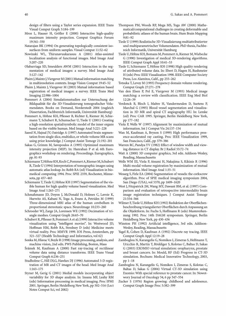
40 G. Sakas and A. Pommert

design of fi lters using a Taylor series expansion. IEEE Trans Visual Comput Graph 3:184–199

Mroz L, Hauser H, Gröller E (2000) Interactive high-quality maximum intensity projection. Comput Graphics Forum 19:341–350

Natarajan BK (1994) On generating topologically consistent iso-surfaces from uniform samples. Visual Comput 11:52–62

Nowinski WL, Thirunavuukarasuu A (2001) Atlas-assisted localization analysis of functional images. Med Image Anal 5:207–220

Olabarriaga SD, Smeulders AWM (2001) Interaction in the seg-mentation of medical images: a survey. Med Image Anal 5:127–142

Pluim J, Maintz J, Viergever M (2001) Mutual information matching in multiresolution contexts. Image Vision Comput 19:45–52

Pluim J, Maintz J, Viergever M (2003) Mutual information based registration of medical images: a survey. IEEE Trans Med Imaging 22:986–1004

Pommert A (2004) Simulationsstudien zur Untersuchung der Bildqualität für die 3D-Visualisierung tomografi scher Volu-mendaten. Books on Demand, Norderstedt 2004 (zugleich Dissertation, Fachbereich Informatik, Universität Hamburg)

Pommert A, Höhne KH, Pfl esser B, Richter E, Riemer M, Schie-mann T, Schubert R, Schumacher U, Tiede U (2001) Creating a high-resolution spatial/symbolic model of the inner organs based on the visible human. Med Image Anal 5:221–228

Saeed N, Hajnal JV, Oatridge A (1997) Automated brain segmen-tation from single slice, multislice, or whole-volume MR scans using prior knowledge. J Comput Assist Tomogr 21:192–201

Sakas G, Grimm M, Savopoulos A (1995) Optimized maximum intensity projection (MIP). In: Hanrahan P et al. 6th Euro-graphics workshop on rendering. Proceedings. Eurographics, pp. 81-93

Schiemann T, Höhne KH, Koch C, Pommert A, Riemer M, Schubert R, Tiede U (1994) Interpretation of tomographic images using automatic atlas lookup. In: Robb RA (ed) Visualization in bio-medical computing 1994. Proc SPIE 2359, Rochester, Minne-sota, pp 457–465

Schiemann T, Tiede U, Höhne KH (1997) Segmentation of the vis-ible human for high quality volume based visualization. Med Image Anal 1:263–271

Schmahmann JD, Doyon J, McDonald D, Holmes C, Lavoie K, Hurwitz AS, Kabani N, Toga A, Evans A, Petrides M (1999) Three-dimensional MRI atlas of the human cerebellum in proportional stereotaxic space. NeuroImage 10:233–260

Schroeder WJ, Zarge JA, Lorensen WE (1992) Decimation of tri-angle meshes. Comput Graph 26:65–70

Schubert R, Pfl esser B, Pommert A et al.(1999) Interactive volume visualization using "intelligent movies". In: Westwood JD, Hoffman HM, Robb RA, Stredney D (eds) Medicine meets virtual reality. Proc MMVR 1999. IOS Press, Amsterdam, pp 321–327 (Health Technology and Informatics, vol 62)

Sonka M, Hlavac V, Boyle R (1998) Image processing, analysis, and machine vision, 2nd edn. PWS Publishing, Boston, Mass

Šrámek M, Kaufman A (2000) Fast ray-tracing of rectilinear volume data using distance transforms. IEEE Trans Visual Comput Graph 6:236–251

Studholme C, Hill DLG, Hawkes DJ (1996) Automated 3-D regis-tration of MR and CT images of the head. Med Image Anal 1:163–175

Styner M, Gerig G (2001) Medial models incorporating object variability for 3D shape analysis. In: Insana MF, Leahy RM (eds) Information processing in medical imaging. Proc IPMI 2001. Springer, Berlin Heidelberg New York, pp 502–516 (Lect Notes Comput Sci, vol 2082)

Thompson PM, Woods RP, Mega MS, Toga AW (2000) Mathe-matical/computational challenges in creating deformable and probabilistic atlases of the human brain. Hum Brain Mapping 9:81–92

Tiede U (1999) Realistische 3D-Visualisierung multiattributierter und multiparametrischer Volumendaten. PhD thesis, Fachbe-reich Informatik, Universität Hamburg

Tiede U, Höhne KH, Bomans M, Pommert A, Riemer M, Wiebecke G (1990) Investigation of medical 3D-rendering algorithms. IEEE Comput Graph Appl 10:41–53

Tiede U, Schiemann T, Höhne KH (1998) High quality rendering of attributed volume data. In: Ebert D, Hagen H, Rushmeier H (eds) Proc IEEE Visualization 1998. IEEE Computer Society Press, Los Alamitos, Calif., pp 255–262

Totsuka T, Levoy M (1993) Frequency domain volume rendering. Comput Graph 27:271–278

Van den Elsen P, Pol E, Viergever M (1993) Medical image matching: a review with classifi cation. IEEE Eng Med Biol 12:26–39

Verdonck B, Bloch I, Maître H, Vandermeulen D, Suetens P, Marchal G (1995) Blood vessel segmentation and visualiza-tion in 3D MR and spiral CT angiography HU. In: Lemke (ed) Proc CAR 1995. Springer, Berlin Heidelberg New York, pp 177–182

Viola P, Wells W (1997) Alignment by maximization of mutual information. Int J Comput Vis 24:137–154

Wan M, Kaufman A, Bryson S (1999) High performance pres-ence-accelerated ray casting. Proc IEEE Visualization 1999, San Francisco, Calif., pp 379–386

Warren RC, Pandya YV (1982) Effect of window width and view-ing distance in CT display. Br J Radiol 55:72–74

Watt A (2000) 3D computer graphics, 3rd edn. Addison-Wesley, Reading, Massachusetts

Wells WM III, Viola P, Atsumi H, Nakajima S, Kikinis R (1996) Multi-modal volume registration by maximization of mutual information. Med Image Anal 1:35–51

Wesarg S, Firle EA (2004) Segmentation of vessels: the corkscrew algorithm. Proc of SPIE medical imaging symposium 2004, San Diego (USA), vol 5370, pp 1609–1620

West J, Fitzpatrick JM, Wang MY, Dawant BM, et al. (1997) Com-parison and evaluation of retrospective intermodality brain image registration techniques. J Comput Assist Tomogr 21:554–566

Wilmer F, Tiede U, Höhne KH (1992) Reduktion der Oberfl ächen-beschreibung triangulierter Oberfl ächen durch Anpassung an die Objektform. In: Fuchs S, Hoffmann R (eds) Mustererken-nung 1992. Proc 14th DAGM symposium. Springer, Berlin Heidelberg New York, pp 430–436

Winston PH (1992) Artifi cial intelligence, 3rd edn. Addison-Wesley, Reading, Massachusetts

Yagel R, Cohen D, Kaufman A (1992) Discrete ray tracing. IEEE Comput Graph Appl 12:19–28

Zamboglou N, Karangelis G, Nomikos I, Zimeras S, Helfmann T, Uricchio R, Martin T, Röddiger S, Kolotas C, Baltas D, Sakas G (2003) EXOMIO virtual simulation: oropharynx, prostate and breast cancers. In: Mould, RF (Ed) Progress in CT-3D simulation. Bochum: Medical Innovative Technology, 2003, pp 1–18

Zamboglou N, Karangelis G, Nomikos I, Zimeras S, Kolotas C, Baltas D, Sakas G (2004) Virtual CT-3D simulation using Exomio: With special reference to prostate cancer. In: Nowot-wory Journal of Oncology 54, 6 pp 547–554

Zucker S (1976) Region growing: childhood and adolesence. Comput Graph Image Proc 5:382–399

Image Registration and Data Fusion for Radiotherapy Treatment Planning 41

5 Image Registration and Data Fusion for Radiotherapy Treatment Planning Marc L. Kessler and Michael Roberson

M. L. Kessler, PhD, ProfessorM. Roberson, BSDepartment of Radiation Oncology The University of Michigan Medical School 1500 East Medical Center DriveAnn Arbor, MI 48109-0010USA

5.1 Introduction

Treatment planning for conformal radiotherapy re-quires accurate delineation of tumor volumes and surrounding healthy tissue. This is especially true in inverse planning where trade-offs in the dose-vol-ume relationships of different tissues are usually the driving forces in the search for an optimal plan. In these situations, slight differences in the shape and overlap regions between a target volume and criti-cal structures can result in different optimized plans. While X-ray computed tomography (CT) remains the primary imaging modality for structure deline-ation, beam placement and generation of digitally reconstructed radiographs, data from other modali-ties, such as magnetic resonance imaging and spec-troscopy (MRI/MRSI) and positron/single photon emission tomography (PET/SPECT), are becoming increasingly prevalent for tumor and normal tissue delineation (Fig. 5.1).

There are many reasons to include image data from other modalities into the treatment-planning process. In many sites, MRI provides superior soft tissue contrast relative to CT and can be used to en-hance or suppress different tissues such as fat and conditions such as edema. Magnetic resonance im-aging also permits imaging along arbitrary planes which can improve visualization and segmentation of different anatomic structures. More recently, MRI has been used to acquire localized informa-tion about relative metabolite concentrations, fl uid mobility, and tissue microstructure. With a variety of tracer compounds available, PET and SPECT can provide unique information about different cellular and physiologic processes to help assess normal and diseased tissues.

In addition to static treatment planning, volu-metric image data is playing a larger role in treat-ment delivery and adaptive radiotherapy. Modern treatment machines can now be equipped with imaging devices that allow acquisition of volumet-ric CT data at the time of treatment. These “treat-ment-delivery CT” studies can be used to adapt a treatment plan based on the patient’s anatomy at the time of treatment and allow more accurate tracking of delivered dose. Furthermore, data from magnetic resonance and nuclear medicine acquired during the course of therapy may also help assess the effi cacy of therapy and indicate prescription changes (Chenevert et al. 2000; Mardor et al. 2003; Barthel et al. 2003; Brun et al. 2002; Allal et al. 2004).

To fully realize the benefi ts of the information available from different imaging studies, the data they provide must be mapped to a single coordinate system, typically that of the treatment planning CT. This process is called image registration. Once they are all linked to a common coordinate system, data can be transferred between studies and integrated to help construct a more complete and accurate repre-sentation of the patient. This process is called data fu-sion. This chapter describes the mechanics of image registration and data fusion processes.

CONTENTS

5.1 Introduction 415.2 Image Registration 425.2.1 Geometric Transformations 435.2.2 Registration Metrics 455.3 Data Fusion 495.4 Validation 515.5 Conclusion 52 References 52

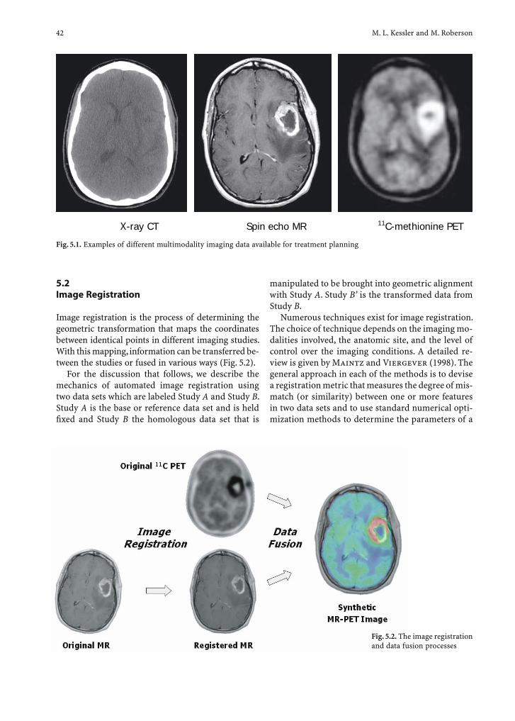
42 M. L. Kessler and M. Roberson

5.2 Image Registration

Image registration is the process of determining the geometric transformation that maps the coordinates between identical points in different imaging studies. With this mapping, information can be transferred be-tween the studies or fused in various ways (Fig. 5.2).

For the discussion that follows, we describe the mechanics of automated image registration using two data sets which are labeled Study A and Study B. Study A is the base or reference data set and is held fi xed and Study B the homologous data set that is

manipulated to be brought into geometric alignment with Study A. Study B’ is the transformed data from Study B.

Numerous techniques exist for image registration. The choice of technique depends on the imaging mo-dalities involved, the anatomic site, and the level of control over the imaging conditions. A detailed re-view is given by Maintz and Viergever (1998). The general approach in each of the methods is to devise a registration metric that measures the degree of mis-match (or similarity) between one or more features in two data sets and to use standard numerical opti-mization methods to determine the parameters of a

Fig. 5.1. Examples of different multimodality imaging data available for treatment planning

Fig. 5.2. The image registration and data fusion processes

x-ray CT Spin echo MR 11C-methionine PET X

Image Registration and Data Fusion for Radiotherapy Treatment Planning 43

geometric transformation that minimize (maximize) the metric. Differences between various techniques include the metric used, the features used to measure the mismatch, the particular form of the geometric transformation used, and the optimization method used for computing the required parameters.

The image registration process illustrated in Fig. 5.3 can be either automated or manual. Automated image registration is analogous to inverse treatment plan-ning, with the registration metric replacing the “plan cost function” and the parameters of the transfor-mation replacing the plan defi ning parameters such as beamlet intensities or weights. In both cases the parameters are iterated using an optimizer until an “optimal” set of parameters is found. Manual image registration is more like forward treatment planning. The “optimizer” is a human with a suite of interac-tive tools that let the user perform various image transformations and visualize the results in real time. While manual registration tools typically only sup-port rotation and translation, they can also be used to initialize more complex automated registrations.

5.2.1 Geometric Transformations

The fundamental task of image registration is to fi nd the geometric transformation, T, which maps the co-ordinates of a point in Study A to the coordinates of the corresponding point in Study B. In general, this transformation can be written as

xB = T (xA,{ }),

where xA is the coordinate of the point in Study A, xB is the coordinate of the same anatomic point in Study

B, and { } is the set of parameters of the transfor-mation. The output of the image registration process is the parameters { } for a particular pair of imag-ing studies (Fig. 5.3). The number of parameters re-quired to determine the transformation depends on the form of T, which in turn depends on the clinical site, clinical application, and the modalities involved.

In the ideal case, where the patient is positioned in an identical orientation in the different imaging studies and the scale and center of the coordinate sys-tems coincide, T is simply an identity transformation I and xB = xA for all points in the two imaging stud-ies. This situation most closely exists for combined imaging modality devices such as PET–CT machines, especially if physiologic motion is controlled or ab-sent. Unfortunately, it is far more common for the orientation of the patient to change between imaging studies, making more sophisticated transformations necessary.

For situations where the anatomy of interest can be assumed to move as a rigid body, the set of param-eters consists of three rotation angles ( x, y, z) and three translations (tx ,ty ,tz). The rigid body transfor-mation is then written as

xB = Trigid (xA, { }) = A xA+b,

where A is a 3×3 rotation matrix and b is a 3×1 trans-lation vector. This transformation is simply the famil-iar one dimensional function “y = m·x+b”, except in three dimensions.

In matrix notation this can be written as

xB

yB

zB

xA

yA

zA

= +A b .

Fig. 5.3. The image registra-tion process

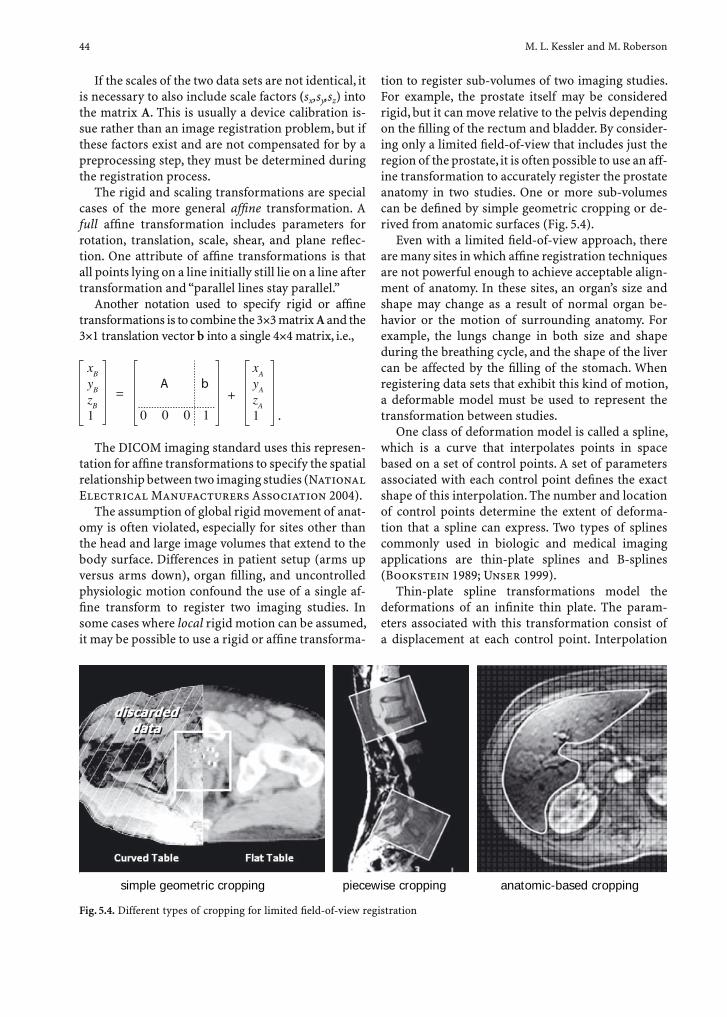
44 M. L. Kessler and M. Roberson

If the scales of the two data sets are not identical, it is necessary to also include scale factors (sx,sy,sz) into the matrix A. This is usually a device calibration is-sue rather than an image registration problem, but if these factors exist and are not compensated for by a preprocessing step, they must be determined during the registration process.

The rigid and scaling transformations are special cases of the more general affi ne transformation. A full affi ne transformation includes parameters for rotation, translation, scale, shear, and plane refl ec-tion. One attribute of affi ne transformations is that all points lying on a line initially still lie on a line after transformation and “parallel lines stay parallel.”

Another notation used to specify rigid or affi ne transformations is to combine the 3×3 matrix A and the 3×1 translation vector b into a single 4×4 matrix, i.e.,

xB

yB

zB

1

= +A b

xA

yA

zA

10 0 0 1 .

The DICOM imaging standard uses this represen-tation for affi ne transformations to specify the spatial relationship between two imaging studies (National Electrical Manufacturers Association 2004).

The assumption of global rigid movement of anat-omy is often violated, especially for sites other than the head and large image volumes that extend to the body surface. Differences in patient setup (arms up versus arms down), organ fi lling, and uncontrolled physiologic motion confound the use of a single af-fi ne transform to register two imaging studies. In some cases where local rigid motion can be assumed, it may be possible to use a rigid or affi ne transforma-

tion to register sub-volumes of two imaging studies. For example, the prostate itself may be considered rigid, but it can move relative to the pelvis depending on the fi lling of the rectum and bladder. By consider-ing only a limited fi eld-of-view that includes just the region of the prostate, it is often possible to use an aff-ine transformation to accurately register the prostate anatomy in two studies. One or more sub-volumes can be defi ned by simple geometric cropping or de-rived from anatomic surfaces (Fig. 5.4).

Even with a limited fi eld-of-view approach, there are many sites in which affi ne registration techniques are not powerful enough to achieve acceptable align-ment of anatomy. In these sites, an organ’s size and shape may change as a result of normal organ be-havior or the motion of surrounding anatomy. For example, the lungs change in both size and shape during the breathing cycle, and the shape of the liver can be affected by the fi lling of the stomach. When registering data sets that exhibit this kind of motion, a deformable model must be used to represent the transformation between studies.

One class of deformation model is called a spline, which is a curve that interpolates points in space based on a set of control points. A set of parameters associated with each control point defi nes the exact shape of this interpolation. The number and location of control points determine the extent of deforma-tion that a spline can express. Two types of splines commonly used in biologic and medical imaging applications are thin-plate splines and B-splines (Bookstein 1989; Unser 1999).

Thin-plate spline transformations model the deformations of an infi nite thin plate. The param-eters associated with this transformation consist of a displacement at each control point. Interpolation

Fig. 5.4. Different types of cropping for limited fi eld-of-view registration

simple geometric cropping piecewise cropping anatomic-based cropping

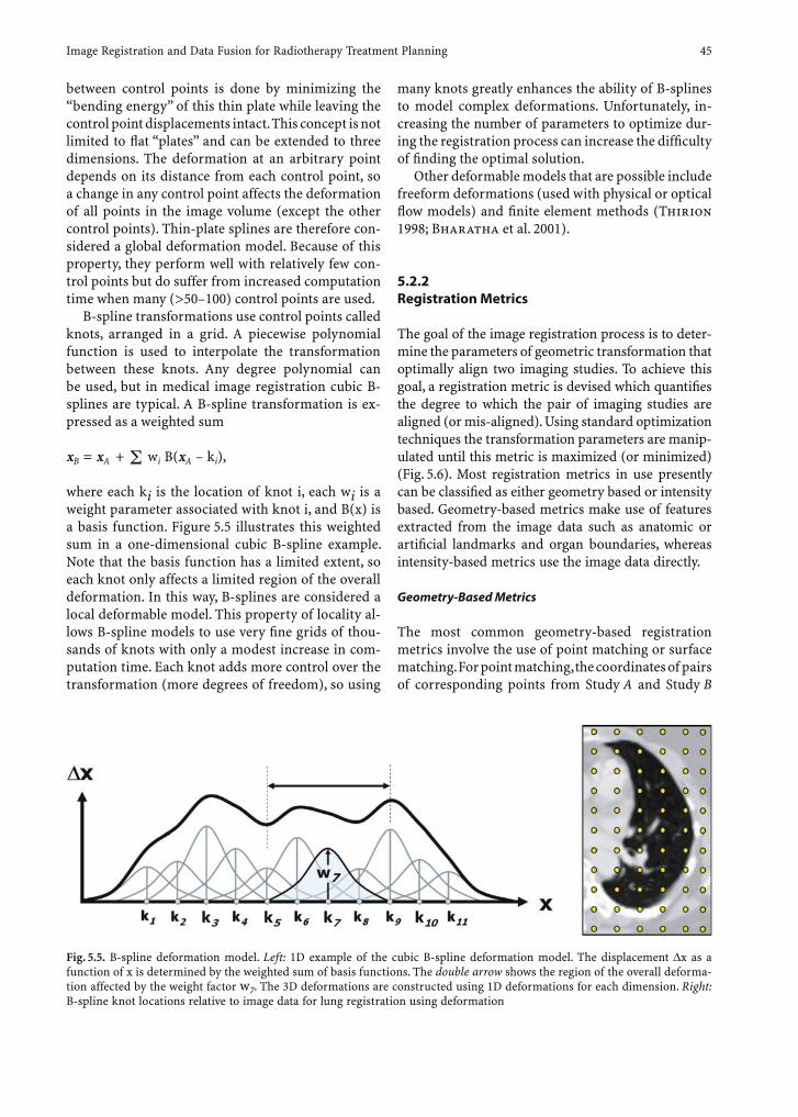
Image Registration and Data Fusion for Radiotherapy Treatment Planning 45

between control points is done by minimizing the “bending energy” of this thin plate while leaving the control point displacements intact. This concept is not limited to fl at “plates” and can be extended to three dimensions. The deformation at an arbitrary point depends on its distance from each control point, so a change in any control point affects the deformation of all points in the image volume (except the other control points). Thin-plate splines are therefore con-sidered a global deformation model. Because of this property, they perform well with relatively few con-trol points but do suffer from increased computation time when many (>50–100) control points are used.

B-spline transformations use control points called knots, arranged in a grid. A piecewise polynomial function is used to interpolate the transformation between these knots. Any degree polynomial can be used, but in medical image registration cubic B-splines are typical. A B-spline transformation is ex-pressed as a weighted sum

xB = xA + wi B(xA – ki),

where each ki is the location of knot i, each wi is a weight parameter associated with knot i, and B(x) is a basis function. Figure 5.5 illustrates this weighted sum in a one-dimensional cubic B-spline example. Note that the basis function has a limited extent, so each knot only affects a limited region of the overall deformation. In this way, B-splines are considered a local deformable model. This property of locality al-lows B-spline models to use very fi ne grids of thou-sands of knots with only a modest increase in com-putation time. Each knot adds more control over the transformation (more degrees of freedom), so using

many knots greatly enhances the ability of B-splines to model complex deformations. Unfortunately, in-creasing the number of parameters to optimize dur-ing the registration process can increase the diffi culty of fi nding the optimal solution.

Other deformable models that are possible include freeform deformations (used with physical or optical fl ow models) and fi nite element methods (Thirion 1998; Bharatha et al. 2001).

5.2.2 Registration Metrics

The goal of the image registration process is to deter-mine the parameters of geometric transformation that optimally align two imaging studies. To achieve this goal, a registration metric is devised which quantifi es the degree to which the pair of imaging studies are aligned (or mis-aligned). Using standard optimization techniques the transformation parameters are manip-ulated until this metric is maximized (or minimized) (Fig. 5.6). Most registration metrics in use presently can be classifi ed as either geometry based or intensity based. Geometry-based metrics make use of features extracted from the image data such as anatomic or artifi cial landmarks and organ boundaries, whereas intensity-based metrics use the image data directly.

Geometry-Based Metrics

The most common geometry-based registration metrics involve the use of point matching or surface matching. For point matching, the coordinates of pairs of corresponding points from Study A and Study B

Fig. 5.5. B-spline deformation model. Left: 1D example of the cubic B-spline deformation model. The displacement ∆x as a function of x is determined by the weighted sum of basis functions. The double arrow shows the region of the overall deforma-tion affected by the weight factor w7. The 3D deformations are constructed using 1D deformations for each dimension. Right: B-spline knot locations relative to image data for lung registration using deformation

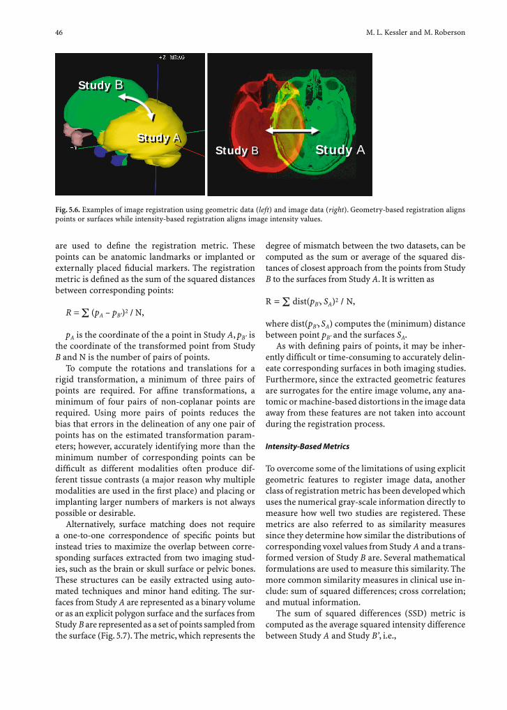
46 M. L. Kessler and M. Roberson

are used to defi ne the registration metric. These points can be anatomic landmarks or implanted or externally placed fi ducial markers. The registration metric is defi ned as the sum of the squared distances between corresponding points:

R = (pA – pB’)2 / N,

pA is the coordinate of the a point in Study A, pB’ is the coordinate of the transformed point from Study B and N is the number of pairs of points.

To compute the rotations and translations for a rigid transformation, a minimum of three pairs of points are required. For affi ne transformations, a minimum of four pairs of non-coplanar points are required. Using more pairs of points reduces the bias that errors in the delineation of any one pair of points has on the estimated transformation param-eters; however, accurately identifying more than the minimum number of corresponding points can be diffi cult as different modalities often produce dif-ferent tissue contrasts (a major reason why multiple modalities are used in the fi rst place) and placing or implanting larger numbers of markers is not always possible or desirable.

Alternatively, surface matching does not require a one-to-one correspondence of specifi c points but instead tries to maximize the overlap between corre-sponding surfaces extracted from two imaging stud-ies, such as the brain or skull surface or pelvic bones. These structures can be easily extracted using auto-mated techniques and minor hand editing. The sur-faces from Study A are represented as a binary volume or as an explicit polygon surface and the surfaces from Study B are represented as a set of points sampled from the surface (Fig. 5.7). The metric, which represents the

degree of mismatch between the two datasets, can be computed as the sum or average of the squared dis-tances of closest approach from the points from Study B to the surfaces from Study A. It is written as

R = dist(pB’, SA)2 / N,

where dist(pB’, SA) computes the (minimum) distance between point pB’ and the surfaces SA.

As with defi ning pairs of points, it may be inher-ently diffi cult or time-consuming to accurately delin-eate corresponding surfaces in both imaging studies. Furthermore, since the extracted geometric features are surrogates for the entire image volume, any ana-tomic or machine-based distortions in the image data away from these features are not taken into account during the registration process.

Intensity-Based Metrics

To overcome some of the limitations of using explicit geometric features to register image data, another class of registration metric has been developed which uses the numerical gray-scale information directly to measure how well two studies are registered. These metrics are also referred to as similarity measures since they determine how similar the distributions of corresponding voxel values from Study A and a trans-formed version of Study B are. Several mathematical formulations are used to measure this similarity. The more common similarity measures in clinical use in-clude: sum of squared differences; cross correlation; and mutual information.

The sum of squared differences (SSD) metric is computed as the average squared intensity difference between Study A and Study B’, i.e.,

Study BStudy B

Study AStudy A

Study BStudy B

Study AStudy A

Fig. 5.6. Examples of image registration using geometric data (left) and image data (right). Geometry-based registration aligns points or surfaces while intensity-based registration aligns image intensity values.

Study AStudy AStudy BStudy B Study AStudy AStudy BStudy B

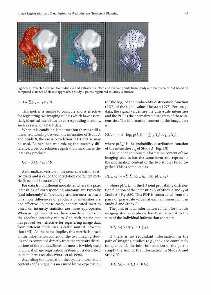
Image Registration and Data Fusion for Radiotherapy Treatment Planning 47

SSD = (IA – IB’)2 / N.

This metric is simple to compute and is effective for registering two imaging studies which have essen-tially identical intensities for corresponding anatomy, such as serial or 4D CT data.

When this condition is not met but there is still a linear relationship between the intensities of Study A and Study B, the cross correlation (CC) metric may be used. Rather than minimizing the intensity dif-ference, cross correlation registration maximizes the intensity product:

CC = (IA * IB’) / N.

A normalized version of the cross correlation met-ric exists and is called the correlation coeffi cient met-ric (Kim and Fessler 2004).

For data from different modalities where the pixel intensities of corresponding anatomy are typically (and inherently) different, registration metrics based on simple differences or products of intensities are not effective. In these cases, sophisticated metrics based on intensity statistics are more appropriate. When using these metrics, there is no dependence on the absolute intensity values. One such metric that has proved very effective for registering image data from different modalities is called mutual informa-tion (MI). As the name implies, this metric is based on the information content of the two imaging stud-ies and is computed directly from the intensity distri-butions of the studies. Since this metric is widely used in clinical image registration systems, it is described in detail here (see also Wells et al. 1996).

According to information theory, the information content H of a “signal” is measured by the expectation

(of the log) of the probability distribution function (PDF) of the signal values (Roman 1997). For image data, the signal values are the gray-scale intensities and the PDF is the normalized histogram of these in-tensities. The information content in the image data is

H(IA) = – E [log2 p(IA)] = - p(IA) log2 p(IA),

where p(IA) is the probability distribution function of the intensities IA of Study A (Fig. 5.8).

The joint or combined information content of two imaging studies has the same form and represents the information content of the two studies fused to-gether. This is computed as

H(IA, IB’) = – p(IA, IB’) log2 p(IA, IB’)

where p(IA, IB’) is the 2D joint probability distribu-tion function of the intensities IA of Study A and IB’ of Study B’ (Fig. 5.9). This PDF is constructed from the pairs of gray-scale values at each common point in Study A and Study B’.

The joint or total information content for the two imaging studies is always less than or equal to the sum of the individual information contents:

H(IA,IB’) ≤ H(IA) + H(IB’).

If there is no redundant information in the pair of imaging studies (e.g., they are completely independent), the joint information of the pair is simply the sum of the information in Study A and Study B’:

H(IA,IB’) = H(IA) + H(IB’).

Fig. 5.7. a Extracted surface from Study A and extracted surface and surface points from Study B. b Points colorized based on computed distance of closest approach. c Study B points registered to Study A surface

ba c

48 M. L. Kessler and M. Roberson

If there is some redundant information, then the joint information content will be less than the sum of the information in the two studies:

H(IA,IB’) < H(IA) + H(IB’).

The amount of shared or mutual information is just the difference between the sum of the individual infor-mation contents and the joint information content,

MI(IA,IB’) = H(IA) + H(IB’) – H(IA,IB’).

Solving for MI from the above equations,

MI(IA,IB’) = p(IA,IB’) log2 [p(IA,IB’) / p(IA’) p(IB’)].

The mutual information between two imag-ing studies can be thought of as the information in Study B’ that is also present in Study A. Accordingly,

one way to describe mutual information is as the amount of information in Study B’ that can be de-termined (or predicted) from Study A. To completely predict Study B’ from Study A, each intensity value in Study A must correspond to exactly one intensity value in Study B’. When this is the case the joint in-tensity histogram has the same distribution as the histogram of Study A, and H(IA,IB’) equals H(IA). The MI is therefore equal to H(IB’), and Study B’ at this point can be thought of as a “recolored” version of Study A.

A major advantage of mutual information is that it is robust to missing or incomplete information. For ex-ample, a tumor might show up clearly on an MR study but be indistinct on a corresponding CT study. Over the tumor volume the mutual information is low, but no prohibitive penalties are incurred. In the surrounding healthy tissue the mutual information can be high, and this becomes the dominant factor in the registration.

Fig. 5.9. Two-dimensional joint-intensity histogram constructed from an MR scan (Study A) and a transformed (reformatted) CT (Study B’)

Fig. 5.8. Left: 3D image volume; Right: probability density function of the image intensities

air

fat

bonetissue

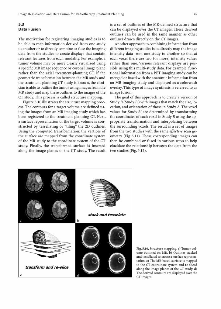
Image Registration and Data Fusion for Radiotherapy Treatment Planning 49

5.3 Data Fusion

The motivation for registering imaging studies is to be able to map information derived from one study to another or to directly combine or fuse the imaging data from the studies to create displays that contain relevant features from each modality. For example, a tumor volume may be more clearly visualized using a specifi c MR image sequence or coronal image plane rather than the axial treatment-planning CT. If the geometric transformation between the MR study and the treatment-planning CT study is known, the clini-cian is able to outline the tumor using images from the MR study and map these outlines to the images of the CT study. This process is called structure mapping.

Figure 5.10 illustrates the structure mapping proc-ess. The contours for a target volume are defi ned us-ing the images from an MR imaging study which has been registered to the treatment-planning CT. Next, a surface representation of the target volume is con-structed by tessellating or “tiling” the 2D outlines. Using the computed transformation, the vertices of the surface are mapped from the coordinate system of the MR study to the coordinate system of the CT study. Finally, the transformed surface is inserted along the image planes of the CT study. The result

is a set of outlines of the MR-defi ned structure that can be displayed over the CT images. These derived outlines can be used in the same manner as other outlines drawn directly on the CT images.

Another approach to combining information from different imaging studies is to directly map the image intensity data from one study to another so that at each voxel there are two (or more) intensity values rather than one. Various relevant displays are pos-sible using this multi-study data. For example, func-tional information from a PET imaging study can be merged or fused with the anatomic information from an MR imaging study and displayed as a colorwash overlay. This type of image synthesis is referred to as image fusion.

The goal of this approach is to create a version of Study B (Study B’) with images that match the size, lo-cation, and orientation of those in Study A. The voxel values for Study B’ are determined by transforming the coordinates of each voxel in Study B using the ap-propriate transformation and interpolating between the surrounding voxels. The result is a set of images from the two studies with the same effective scan ge-ometry (Fig. 5.11). These corresponding images can then be combined or fused in various ways to help elucidate the relationship between the data from the two studies (Fig. 5.12).

Fig. 5.10. Structure mapping. a) Tumor vol-ume outlined on MR. b) Outlines stacked and tessellated to create a surface represen-tation. c) The MR-based surface is mapped to the CT coordinate system and re-sliced along the image planes of the CT study. d) The derived contours are displayed over the CT images.

a

d

b

c

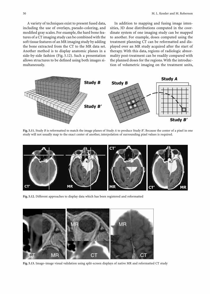
50 M. L. Kessler and M. Roberson

A variety of techniques exist to present fused data, including the use of overlays, pseudo-coloring, and modifi ed gray scales. For example, the hard bone fea-tures of a CT imaging study can be combined with the soft tissue features of an MR imaging study by adding the bone extracted from the CT to the MR data set. Another method is to display anatomic planes in a side-by-side fashion (Fig. 5.12). Such a presentation allows structures to be defi ned using both images si-multaneously.

In addition to mapping and fusing image inten-sities, 3D dose distributions computed in the coor-dinate system of one imaging study can be mapped to another. For example, doses computed using the treatment planning CT can be reformatted and dis-played over an MR study acquired after the start of therapy. With this data, regions of radiologic abnor-mality post-treatment can be readily compared with the planned doses for the regions. With the introduc-tion of volumetric imaging on the treatment units,

Fig. 5.11. Study B is reformatted to match the image planes of Study A to produce Study B’. Because the center of a pixel in one study will not usually map to the exact center of another, interpolation of surrounding pixel values is required.

Fig. 5.12. Different approaches to display data which has been registered and reformatted

Fig. 5.13. Image–image visual validation using split-screen displays of native MR and reformatted CT study

CT CT CT

MR MR

MR

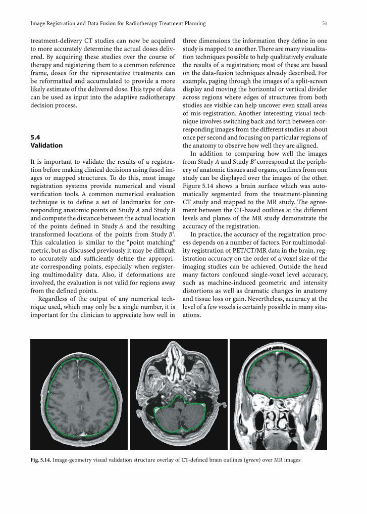
Image Registration and Data Fusion for Radiotherapy Treatment Planning 51

treatment-delivery CT studies can now be acquired to more accurately determine the actual doses deliv-ered. By acquiring these studies over the course of therapy and registering them to a common reference frame, doses for the representative treatments can be reformatted and accumulated to provide a more likely estimate of the delivered dose. This type of data can be used as input into the adaptive radiotherapy decision process.

5.4 Validation

It is important to validate the results of a registra-tion before making clinical decisions using fused im-ages or mapped structures. To do this, most image registration systems provide numerical and visual verifi cation tools. A common numerical evaluation technique is to defi ne a set of landmarks for cor-responding anatomic points on Study A and Study B and compute the distance between the actual location of the points defi ned in Study A and the resulting transformed locations of the points from Study B’. This calculation is similar to the “point matching” metric, but as discussed previously it may be diffi cult to accurately and suffi ciently defi ne the appropri-ate corresponding points, especially when register-ing multimodality data. Also, if deformations are involved, the evaluation is not valid for regions away from the defi ned points.

Regardless of the output of any numerical tech-nique used, which may only be a single number, it is important for the clinician to appreciate how well in

three dimensions the information they defi ne in one study is mapped to another. There are many visualiza-tion techniques possible to help qualitatively evaluate the results of a registration; most of these are based on the data-fusion techniques already described. For example, paging through the images of a split-screen display and moving the horizontal or vertical divider across regions where edges of structures from both studies are visible can help uncover even small areas of mis-registration. Another interesting visual tech-nique involves switching back and forth between cor-responding images from the different studies at about once per second and focusing on particular regions of the anatomy to observe how well they are aligned.

In addition to comparing how well the images from Study A and Study B’ correspond at the periph-ery of anatomic tissues and organs, outlines from one study can be displayed over the images of the other. Figure 5.14 shows a brain surface which was auto-matically segmented from the treatment-planning CT study and mapped to the MR study. The agree-ment between the CT-based outlines at the different levels and planes of the MR study demonstrate the accuracy of the registration.

In practice, the accuracy of the registration proc-ess depends on a number of factors. For multimodal-ity registration of PET/CT/MR data in the brain, reg-istration accuracy on the order of a voxel size of the imaging studies can be achieved. Outside the head many factors confound single-voxel level accuracy, such as machine-induced geometric and intensity distortions as well as dramatic changes in anatomy and tissue loss or gain. Nevertheless, accuracy at the level of a few voxels is certainly possible in many situ-ations.

Fig. 5.14. Image-geometry visual validation structure overlay of CT-defi ned brain outlines (green) over MR images

52 M. L. Kessler and M. Roberson

5.5 Conclusion

Accurate delineation of tumor volumes and critical structures is a vital component of treatment plan-ning. The use of a single imaging study to perform the delineation is not always adequate and multiple studies may need to be combined. In order to use data from multiple studies, the spatial alignment of the studies must be determined. Image registration, the process of fi nding a coordinate transformation between two studies, can recover rigid, affi ne, and deformed transformations. Automatic registration requires a similarity measure or registration metric. The metric may be specialized for particular types of registration (e.g., single modality) or may be gener-ally applicable. Manual registration can use a metric as well, or it can be based on interactive visual in-spection. Deformations are generally not manually registered. Once the coordinate transformation be-tween the imaging studies has been found, various structure mapping and data fusion techniques can be used to integrate the data. Before the resulting data is used in the clinic, a validation process should take place. This might include numerical measure-ments such as comparisions of landmark positions, but should always include a visual inspection across the entire data set.

The techniques described in this chapter are tools to help use the information from different imaging studies in a common geometric framework. These techniques apply to both time-series single modal-ity and multimodality imaging studies. Most modern radiotherapy treatment planning systems support the use of functional as well as multimodality ana-tomic imaging using one or more of the techniques presented. These tools, however, cannot replace clini-cal judgment. Different imaging modalities image the same tissues differently, and although tools may help us better understand and differentiate between tumor and non-tumor, they cannot yet make the ul-timate decision of what to treat and what not to treat. These decisions still lie with the clinician, although they now have more sophisticated tools to help make these choices.

References

Allal AS, Slosman DO, Kebdani T, Allaoua M, Lehmann W, Dul-guerov P (2004) Prediction of outcome in head-and-neck cancer patients using the standardized uptake value of 2-[18F]fl uoro-2-deoxy-D-glucose. Int J Radiat Oncol Biol Phys 59:1295–1300

Barthel H, Cleij MC, Collingridge DR, Hutchinson OC, Osman S, He Q, Luthra SK, Brady F, Price PM, Aboagye EO (2003) 3’-deoxy-3’-[18F]fl uorothymidine as a new marker for monitoring tumor response to antiproliferative therapy in vivo with positron emission tomography. Cancer Res 63:3791–3798

Bharatha A, Hirose M, Hata N, Warfi eld SK, Ferrant M, Zou KH, Suarez-Santana E, Ruiz-Alzola J, D’Amico A, Cormack RA, Kikinis R, Jolesz FA, Tempany CM (2001) Evaluation of three-dimensional fi nite element-based deformable regis-tration of pre- and intraoperative prostate imaging. Med Phys 28:2551–2260

Bookstein FL (1989) Principal warps: thin-plate splines and the decomposition of deformations. IEEE Trans Pattern Anal Mach Intell Vol 11. 6:567–585

Brun E, Kjellen E, Tennvall J, Ohlsson T, Sandell A, Perfekt R, Perfekt R, Wennerberg J, Strand SE (2002) FDG PET studies during treatment: prediction of therapy outcome in head and neck squamous cell carcinoma. Head Neck 24:127–135

Chenevert TL, Stegman LD, Taylor JM, Robertson PL, Green-berg HS, Rehemtulla A, Ross BD (2000) Diffusion mag-netic resonance imaging: an early surrogate marker of therapeutic effi cacy in brain tumors. J Natl Cancer Inst 92:2029–2036

Kim J, Fessler JA (2004) Intensity-based image registration using robust correlation coeffi cients. IEEE Trans Med Imaging 23:1430–1444

Maintz JB, Viergever MA (1998) A survey of medical image registration. Med Image Anal 2:1–36

Mardor Y, Pfeffer R, Spiegelmann R, Roth Y, Maier SE, Nissim O, Berger R, Glicksman A, Baram J, Orenstein A, Cohen JS, Tichler T (2003) Early detection of response to radiation therapy in patients with brain malignancies using conven-tional and high b-value diffusion-weighted magnetic reso-nance imaging. J Clin Oncol 21:1094–1100

National Electrical Manufacturers Association (2004) DICOM, part 3, PS3.3 – service class specifi cations. Rosslyn, Vir-gina

Roman S (1997) Introduction to coding and information theory. Undergraduate texts in mathematics. Springer, Berlin Heidelberg New York

Thirion JP (1998) Image matching as a diffusion process: an analogy with Maxwell’s demons. Med Image Anal 2:243–260

Unser M (1999) Splines: a perfect fi t for signal and image pro-cessing. IEEE Sign Process Mag Vol 16. 6:22–38

Wells WM 3rd, Viola P, Atsumi H, Nakajima S, Kikinis R (1996) Multi-modal volume registration by maximization of mutual information. Med Image Anal Vol 1. 1:35–51

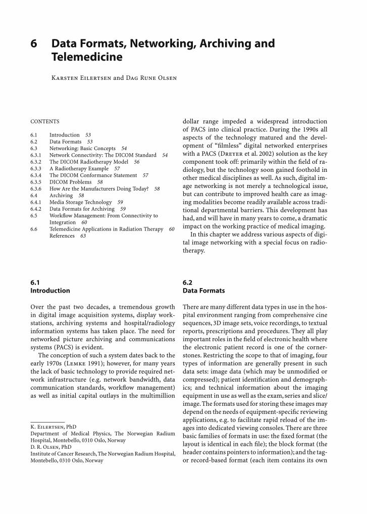
Data Formats, Networking, Archiving and Telemedicine 53

6 Data Formats, Networking, Archiving and Telemedicine

Karsten Eilertsen and Dag Rune Olsen

K. Eilertsen, PhDDepartment of Medical Physics, The Norwegian Radium Hospital, Montebello, 0310 Oslo, NorwayD. R. Olsen, PhDInstitute of Cancer Research, The Norwegian Radium Hospital, Montebello, 0310 Oslo, Norway

6.1 Introduction

Over the past two decades, a tremendous growth in digital image acquisition systems, display work-stations, archiving systems and hospital/radiology information systems has taken place. The need for networked picture archiving and communications systems (PACS) is evident.

The conception of such a system dates back to the early 1970s (Lemke 1991); however, for many years the lack of basic technology to provide required net-work infrastructure (e.g. network bandwidth, data communication standards, workfl ow management) as well as initial capital outlays in the multimillion

dollar range impeded a widespread introduction of PACS into clinical practice. During the 1990s all aspects of the technology matured and the devel-opment of “fi lmless” digital networked enterprises with a PACS (Dreyer et al. 2002) solution as the key component took off: primarily within the fi eld of ra-diology, but the technology soon gained foothold in other medical disciplines as well. As such, digital im-age networking is not merely a technological issue, but can contribute to improved health care as imag-ing modalities become readily available across tradi-tional departmental barriers. This development has had, and will have in many years to come, a dramatic impact on the working practice of medical imaging.

In this chapter we address various aspects of digi-tal image networking with a special focus on radio-therapy.

6.2 Data Formats

There are many different data types in use in the hos-pital environment ranging from comprehensive cine sequences, 3D image sets, voice recordings, to textual reports, prescriptions and procedures. They all play important roles in the fi eld of electronic health where the electronic patient record is one of the corner-stones. Restricting the scope to that of imaging, four types of information are generally present in such data sets: image data (which may be unmodifi ed or compressed); patient identifi cation and demograph-ics; and technical information about the imaging equipment in use as well as the exam, series and slice/image. The formats used for storing these images may depend on the needs of equipment-specifi c reviewing applications, e.g. to facilitate rapid reload of the im-ages into dedicated viewing consoles. There are three basic families of formats in use: the fi xed format (the layout is identical in each fi le); the block format (the header contains pointers to information); and the tag- or record-based format (each item contains its own

CONTENTS

6.1 Introduction 536.2 Data Formats 536.3 Networking: Basic Concepts 546.3.1 Network Connectivity: The DICOM Standard 546.3.2 The DICOM Radiotherapy Model 566.3.3 A Radiotherapy Example 576.3.4 The DICOM Conformance Statement 576.3.5 DICOM Problems 586.3.6 How Are the Manufacturers Doing Today? 586.4 Archiving 586.4.1 Media Storage Technology 596.4.2 Data Formats for Archiving 596.5 Workfl ow Management: From Connectivity to Integration 606.6 Telemedicine Applications in Radiation Therapy 60 References 63

54 K. Eilertsen and D. R. Olsen

length). Extracting image data from such fi les is usu-ally easy, even if a proprietary formatting is used, but to decipher every detail may require detailed insight into the format specifi cation. Examples of standard fi le formats in widespread use are Tagged Image File Format (TIFF), Graphic Interchange Format (GIF), JPEG fi le interchange format (JIFF), MPEG (mov-ies), WAV and MIDI (voices). Recently, the Portable Network Graphic (PNG) has gained popularity, es-pecially for Internet web applications. The stream of DICOM messages stored in a fi le may also be consid-ered an image format and has become a common way of keeping medical images. The reading of such fi les may require detailed knowledge about the streaming syntax and the underlying communication protocols that were used (see below).

Extensive use of different image formats restricts the ability of cross-platform data sharing in a net-worked environment, as dedicated fi le readers and viewers are needed. Important image characteristics, such as resolution, gray and/or color scale interpre-tation, contrast and brightness, may deteriorate or even be lost due to inherent limitations of the for-mat in use. The creation of suffi ciently comprehen-sive image formats and the subsequent network transport from the modality to (any) application in a standardized fashion is therefore a major endeavor. In the next sections we explore one solution to this challenge.

6.3 Networking: Basic Concepts

The International Organization for Standardization has defi ned the Open System Interconnection (OSI) reference model to be used as an architectural frame-work for network communication. The OSI model describes how data in one application is transported trough a network medium to another application. The model concept consists of seven different layers, each layer specifying a particular network function (Table 6.1). The functions of the different layers are fairly self-contained, and the actual implementation of these functions (often called protocols) makes possible the communication or transport of data be-tween the layers.

The design of a PACS network within a particu-lar hospital environment would constitute a typical Local Area Network (LAN) where an Ethernet topol-ogy (or Fast Ethernet, Gigabit Ethernet) with TCP/IP is utilized to facilitate networked communica-

tion. Furthermore, several hospitals within the same health care organization can be connected into Wide-Area Networks (WAN).

Having defi ned the basic framework for network operation, the challenge is to exploit this topology to facilitate smooth connectivity between the multiven-dor modalities.

6.3.1 Network Connectivity: The DICOM Standard

An apparently seamless exchange of data between dif-ferent computer applications (or modalities; Fig. 6.1) in the hospital network has traditionally been re-stricted to vendor-specifi c equipment that applies proprietary standards. In a modern multimodality hospital environment with a multitude of digital sys-tems from many different manufacturers, proprietary solutions offer little fl exibility. They are costly and cumbersome to operate as custom interfaces must be developed and maintained, possibly error prone and safety critical since data consistency can be jeop-ardized as data must be reformatted to suit a given equipment specifi cation. An additional maintenance level may be required to assure data quality when, for instance, equipment is upgraded or replaced. The use of such solutions may therefore represent a serious obstacle to the progress and introduction of state-of-the art network technology.

During the 1980s the need for simplifi cation and standardization became apparent in order to ensure and maintain vital connectivity and interoperabil-ity of all pieces of equipment. The medical equip-ment industry, represented by the National Electrical Manufacturers Association (NEMA) and the medical community, represented by the American College of Radiology (ACR), joined forces to develop the Digital Imaging and Communications in Medicine standard (DICOM). The intention was to create an

Table 6.1. The seven OSI model layers and an OSI model realiza-tion with Ethernet and TCP/IP

Layer OSI model Ethernet with TCP/IP

7 Application Telnet, ftp, SMTP

6 Presentation Data formats (e.g. JPEG, MPEG, ASCII)

5 Session Session Control Protocol (SCP), DECNet

4 Transport Transmission Control Protocol (TCP)

3 Network Internet Protocol (IP)

2 Data link Ethernet Network Interface Card (NIC)

1 Physical Twisted pair CAT 5 cabling, FiberChannel

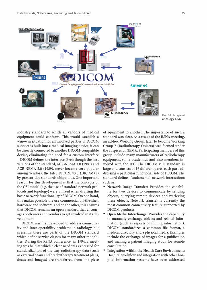
Data Formats, Networking, Archiving and Telemedicine 55

industry standard to which all vendors of medical equipment could conform. This would establish a win–win situation for all involved parties: if DICOM support is built into a medical imaging device, it can be directly connected to another DICOM-compatible device, eliminating the need for a custom interface – DICOM defi nes the interface. Even though the fi rst versions of the standard, ACR-NEMA 1.0 (1985) and ACR-NEMA 2.0 (1989), never became very popular among vendors, the later DICOM v3.0 (DICOM) is by present-day standards ubiquitous. One important reason for this development is that the concepts of the OSI model (e.g. the use of standard network pro-tocols and topology) were utilized when drafting the basic network functionality of DICOM. On one hand, this makes possible the use commercial off-the-shelf hardware and software, and on the other, this ensures that DICOM remains an open standard that encour-ages both users and vendors to get involved in its de-velopment.

DICOM was fi rst developed to address connectiv-ity and inter-operability problems in radiology, but presently there are parts of the DICOM standard which defi ne service classes for many other modali-ties. During the RSNA conference in 1994, a meet-ing was held at which a clear need was expressed for standardization of the way radiotherapy data (such as external beam and brachytherapy treatment plans, doses and images) are transferred from one piece

of equipment to another. The importance of such a standard was clear. As a result of the RSNA meeting, an ad-hoc Working Group, later to become Working Group 7 (Radiotherapy Objects) was formed under the auspices of NEMA. Participating members of this group include many manufacturers of radiotherapy equipment, some academics and also members in-volved with the IEC. The DICOM v3.0 standard is large and consists of 16 different parts, each part ad-dressing a particular functional side of DICOM. The standard defi nes fundamental network interactions such as:• Network Image Transfer: Provides the capabil-

ity for two devices to communicate by sending objects, querying remote devices and retrieving these objects. Network transfer is currently the most common connectivity feature supported by DICOM products.

• Open Media Interchange: Provides the capability to manually exchange objects and related infor-mation (such as reports or fi lming information). DICOM standardizes a common fi le format, a medical directory and a physical media. Examples include the exchange of images for a publication and mailing a patient imaging study for remote consultation.

• Integration within the Health Care Environment: Hospital workfl ow and integration with other hos-pital information systems have been addressed

Fig. 6.1. A typical oncology LAN

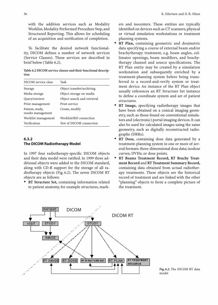
56 K. Eilertsen and D. R. Olsen

with the addition services such as Modality Worklist, Modality Performed Procedure Step, and Structured Reporting. This allows for scheduling of an acquisition and notifi cation of completion.

To facilitate the desired network functional-ity, DICOM defi nes a number of network services (Service Classes). These services are described in brief below (Table 6.2).

ers and isocenters. These entities are typically identifi ed on devices such as CT scanners, physical or virtual simulation workstations or treatment planning systems.

• RT Plan, containing geometric and dosimetric data specifying a course of external beam and/or brachytherapy treatment, e.g. beam angles, col-limator openings, beam modifi ers, and brachy-therapy channel and source specifi cations. The RT Plan entity may be created by a simulation workstation and subsequently enriched by a treatment-planning system before being trans-ferred to a record-and-verify system or treat-ment device. An instance of the RT Plan object usually references an RT Structure Set instance to defi ne a coordinate system and set of patient structures.

• RT Image, specifying radiotherapy images that have been obtained on a conical imaging geom-etry, such as those found on conventional simula-tors and (electronic) portal imaging devices. It can also be used for calculated images using the same geometry, such as digitally reconstructed radio-graphs (DRRs).

• RT Dose, containing dose data generated by a treatment-planning system in one or more of sev-eral formats: three-dimensional dose data; isodose curves; DVHs; or dose points.

• RT Beams Treatment Record, RT Brachy Treat-ment Record and RT Treatment Summary Record, containing data obtained from actual radiother-apy treatments. These objects are the historical record of treatment and are linked with the other “planning” objects to form a complete picture of the treatment.

Table 6.2 DICOM service classes and their functional descrip-tion

DICOM service class Task

Storage Object transfer/archiving

Media storage Object storage on media

Query/retrieve Object search and retrieval

Print management Print service

Patient, study, results management

Create, modify

Worklist management Worklist/RIS connection

Verifi cation Test of DICOM connection

6.3.2 The DICOM Radiotherapy Model

In 1997 four radiotherapy-specifi c DICOM objects and their data model were ratifi ed. In 1999 three ad-ditional objects were added to the DICOM standard, along with CD-R support for the storage of all ra-diotherapy objects (Fig. 6.2). The seven DICOM RT objects are as follows:• RT Structure Set, containing information related

to patient anatomy, for example structures, mark-

Fig. 6.2. The DICOM RT data model

DICOM RTDICOM

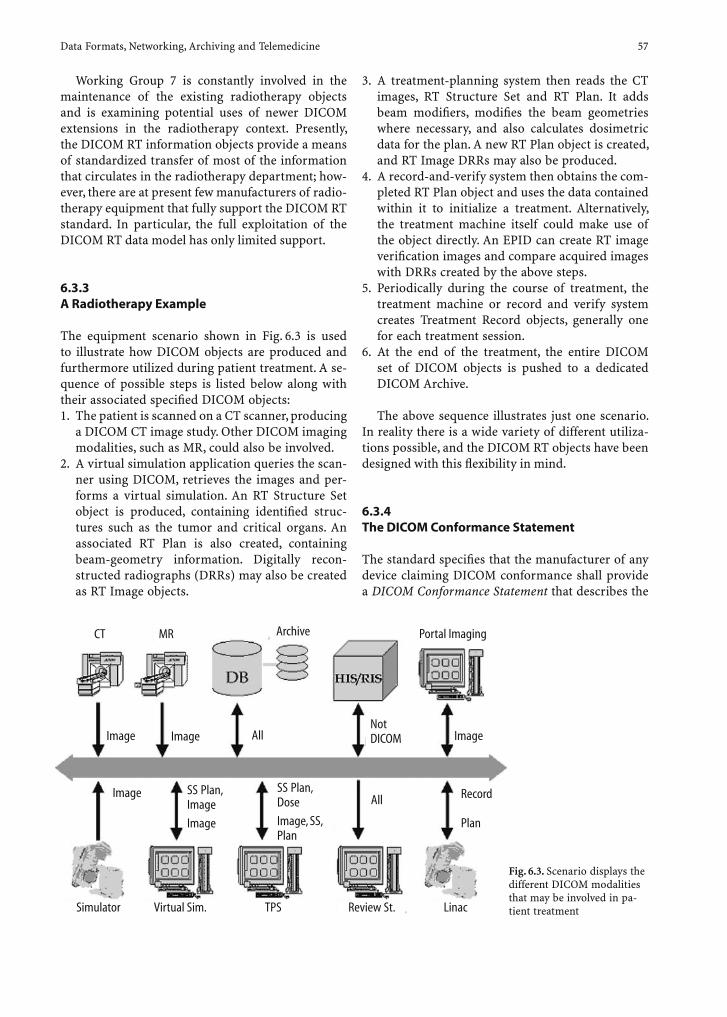
Data Formats, Networking, Archiving and Telemedicine 57

Working Group 7 is constantly involved in the maintenance of the existing radiotherapy objects and is examining potential uses of newer DICOM extensions in the radiotherapy context. Presently, the DICOM RT information objects provide a means of standardized transfer of most of the information that circulates in the radiotherapy department; how-ever, there are at present few manufacturers of radio-therapy equipment that fully support the DICOM RT standard. In particular, the full exploitation of the DICOM RT data model has only limited support.

6.3.3 A Radiotherapy Example

The equipment scenario shown in Fig. 6.3 is used to illustrate how DICOM objects are produced and furthermore utilized during patient treatment. A se-quence of possible steps is listed below along with their associated specifi ed DICOM objects:1. The patient is scanned on a CT scanner, producing

a DICOM CT image study. Other DICOM imaging modalities, such as MR, could also be involved.

2. A virtual simulation application queries the scan-ner using DICOM, retrieves the images and per-forms a virtual simulation. An RT Structure Set object is produced, containing identifi ed struc-tures such as the tumor and critical organs. An associated RT Plan is also created, containing beam-geometry information. Digitally recon-structed radiographs (DRRs) may also be created as RT Image objects.

3. A treatment-planning system then reads the CT images, RT Structure Set and RT Plan. It adds beam modifi ers, modifi es the beam geometries where necessary, and also calculates dosimetric data for the plan. A new RT Plan object is created, and RT Image DRRs may also be produced.

4. A record-and-verify system then obtains the com-pleted RT Plan object and uses the data contained within it to initialize a treatment. Alternatively, the treatment machine itself could make use of the object directly. An EPID can create RT image verifi cation images and compare acquired images with DRRs created by the above steps.

5. Periodically during the course of treatment, the treatment machine or record and verify system creates Treatment Record objects, generally one for each treatment session.

6. At the end of the treatment, the entire DICOM set of DICOM objects is pushed to a dedicated DICOM Archive.

The above sequence illustrates just one scenario. In reality there is a wide variety of different utiliza-tions possible, and the DICOM RT objects have been designed with this fl exibility in mind.

6.3.4 The DICOM Conformance Statement

The standard specifi es that the manufacturer of any device claiming DICOM conformance shall provide a DICOM Conformance Statement that describes the

Fig. 6.3. Scenario displays the different DICOM modalities that may be involved in pa-tient treatment

SS Plan, Dose

Image, SS, Plan

SS Plan, Image

Image

All Record

Plan

ImageAll

Simulator

Portal Imaging

Not DICOMImageImage

Image

CT MR Archive

Virtual Sim. TPS Review St. Linac

58 K. Eilertsen and D. R. Olsen

DICOM capabilities of the device (cf. part 2 of the DICOM standard). Many manufacturers make their conformance statements available on the Internet. Potential connectivity between two pieces of equip-ment can therefore be evaluated in advance by reading Conformance statements which provide a foundation to determine connectivity and assess the potential inter-operability of two products, and in some cases identify potential problems without ever having physically connected them.

It is not suffi cent for a vendor to simply claim con-formance to DICOM. The statement “This product is DICOM” has even less meaning in the radiotherapy domain, in which inter-operability is a very complex issue. For RT applications, it is usually not possible to determine inter-operability a priory – this must be established through extensive testing. Still, radiother-apy professionals should insist upon a conformance statement for any device that claims to be DICOM conformant. Even so, DICOM conformance is vol-untary and there is no authority that approves or may enforce conformance; however, by conforming to DICOM, one can develop safe, reliable computer applications with a high degree of built-in connec-tivity.

6.3.5 DICOM Problems

Even a standard such as DICOM does not completely eliminate connectivity issues, and the inherent fl ex-ibility of the standard is a common source of confu-sion and frustration. The DICOM standard, and the RT parts in particular, contains numerous so-called type-2 and type-3 attributes. Type-2 attributes must be present in a DICOM message for the message to be valid, but the attribute value may be sent empty if unknown, i.e. it is left with the application vendor to fi ll in the value. Type-3 attributes are optional, i.e. they may or may not be present in a message. Some of these attributes can be crucial for the functional-ity of other applications. One example would be the tabletop positions (type 3) in the RT plan. These at-tributes are very useful to ensure a correct setup of the patient during external-beam radiotherapy. The attributes should be provided by the planning system for use by the record and verify system when set-ting up the patient at treatment. Presently, there are very few planning systems that provide these values. Another common problem is the different ways ven-dors organize 3D image sets (CT, MR, etc.) into se-ries. Some applications, such as treatment-planning

systems and virtual simulators, rely on all images of a given type (e.g. all axial images) to exist in the same series in order to create a 3D reconstructed volumetric data representation. Especially older CT/MR scanners tend to split such data sets into several series or even put localizer and axial images in the same series.

6.3.6 How Are the Manufacturers Doing Today?

DICOM is now a mature standard. After a lot of hard work understanding, developing and testing product inter-operability in the radiotherapy context, a large number of manufacturers now have products avail-able that support one or more of the radiotherapy DICOM objects. Vendors who have such products available, or have demonstrated them as works in progress, include Elekta, General Electric Medical Systems, IMPAC, Merge Technologies, Multidata, NOMOS, Nucletron, Picker International, ROCS, Siemens Medical Systems, SSGI, CMS and Varian Medical Systems.

6.4 Archiving

Historically the term “archive” refers to an institu-tion or facility that undertakes the task of preserv-ing records for longer periods of time, sometimes indefi nitely. The core tasks of such an archive are typically to provide means for access control, ensure long-term media stability and readability, and to pre-serve record authenticity, in addition to disaster safe storage. The records in such archives have tradition-ally been data on analogue media such as paper and photographic fi lm that can be visually inspected. This description also applies to medical archives that typi-cally contain patient records and X-ray fi lms.

The growth of information that exists in digital format within the medical environment poses a tremendous challenge to the traditional way of ar-chiving. The main concern is probably the media on which the data is being stored. Media storage tech-nology is evolving rapidly and there is an inherent risk that such media is outdated in a matter of few years (10–20 years) mainly because the hardware and software components required to access the storage media are no longer manufactured and sup-ported.

Data Formats, Networking, Archiving and Telemedicine 59

A fundamental prerequisite for digital archives is therefore that they easily can accommodate new stor-age technology as well as to easily scale with grow-ing demands in capacity. In other words, the archive should have built-in technology that, for instance, facilitates automatic data migration from one media/storage technology to another. The cost of archiving digital information should thus include not only the running costs of technical maintenance and support, but also the cost of keeping up with the continuous changes in technology.

The role of the archives is also changing. Contrary to the historical “archive”, an important feature of a digital archive, is potential ease and speed of access. In a PACS implementation the archive serves as a common location for receiving all images as well as the source for distribution of images. To achieve this, the notions of on-line cache or storage (meaning fast access, low capacity), and long-term or secondary storage (meaning slow access but huge capacity), are often used. The present trend is that that these two concepts tend to merge as the storage media become cheaper.

Another important aspect in the digital archive is reliability and robustness. A common measure of re-liability is a system’s “uptime”, and it is generally ac-cepted that this should be greater than 99% per year, i.e. less than 3.6 days/year downtime. Still, the archive is in essence the hub in the PACS network and, if un-available, production is jeopardized. It is therefore important to invest in hardware and software with built-in redundancy that can mitigate the effect of technology failures. In addition, special procedures and plans should be developed to handle catastrophic events such as fi res, earthquakes, etc., for instance, by establishing remote vaults for off-site data storage.

6.4.1 Media Storage Technology

Storage media has for years enjoyed continuous prog-ress in increased capacity and reduction in prices. This applies to all of the most popular storage media. It makes no sense to quote absolute fi gures as these will soon become dated; however, a crude estimate on a relative scale would roughly be (2004) 1000, 10, 5 and 1, for solid-state memory, magnetic disk, mag-netic tape storage (DLT) and optical storage (DVD), respectively, considering the media price only.

The choice of storage technology is usually a trade-off between storage price/capacity and access time. The faster access times required, the more expensive

the storage. For archiving purposes there has been a tradition to use magnetic disk for the on-line stor-age and optical/magnetic tape for secondary storage; however, advances in both storage and LAN technol-ogy along with lower prices has demonstrated a trend towards extensive use of large-scale magnetic-disk arrays for both on-line as well as long-term storage. The concepts of Network Attached Storage (NAS) and Storage Area Networks (SAN) have furthermore promoted this trend.

6.4.2 Data Formats for Archiving

When using DICOM the problem of different or pro-prietary data formats is reduced to having access to a DICOM object/message viewer. If one cannot use the application that generated the object initially to review the object, there exist several applications – either as freeware or for a small fee – that can be downloaded from the internet to accomplish this task. Some of these viewer applications include built-in DICOM storage providers that can be used to receive the DICOM message. In the fi eld of radio-therapy proper viewers are still scarce probably due to the inherent complexity of the RT DICOM objects and the amount on non-image data.

The demands on the data format used for stor-age in an archive are different. The amount of data to be stored is potentially enormous and many ar-chives apply compression to allow for more data to be stored. From a user’s point of view the archive can be considered a black box that talks DICOM. As long as the archive gives back what once was stored, the user is satisfi ed and the internal storage format of the archive is as such irrelevant; however, if compression is used, the quality of the returned image may be re-duced with respect to the original and this may not be acceptable. The DICOM committee has deemed lossless JPEG and lossy JPEG acceptable techniques for compressing medical images, and several archive vendors have implemented strategies for the use of these techniques. A common option is to make the compression technique in use dependent on the age of the object, i.e. newer objects are only made subject to lossless JPEG (two to three times reduction of most images), whereas older objects are compressed using lossy JPEG (10- to 100-fold reduction in image size). This implies that the archive continuously migrates data from lossless to lossy JPEG. Another strategy is to use different compression techniques for different image types. A noisy 512¥512 radiotherapy portal

60 K. Eilertsen and D. R. Olsen

image may suffer considerable loss in quality if lossy JPEG at a ratio of 10:1 is used, whereas a 4000¥8000 MB chest X-ray may be compressed satisfactorily at a ratio of 60:1. Only careful testing can reveal what is the appropriate compression level.

Evidently, it is important that the user defi nes this strategy in accordance with health care regulations.

6.5 Workfl ow Management: From Connectivity to Integration

The computer network of the hospital should pro-vide the technical infrastructure required for rapid transmission and exchange of data between the dif-ferent modalities used for diagnosis, planning and treatment. The use of DICOM will eventually provide excellent connectivity between the interacting par-ties. But DICOM has as of yet limited support for workfl ow management and data integration. Custom-made solutions may be required, and DICOM was not intended to solve this task.

In order to understand what DICOM can and can-not provide, it is important to distinguish between DICOM connectivity and application interoperability. This is especially true in the domain of radiotherapy where the working process is very dynamic. DICOM connectivity refers to the DICOM message exchange standard responsible for establishing connections and exchanging properly structured messages so that an information object sent from one node will be completely received by the receiving node. In other words, the successful transfer of information: the successful “plug and exchange” between two pieces of equipment.

Beyond connectivity lies application interoper-ability: the ability to process and manipulate infor-mation objects. DICOM radiotherapy objects play a crucial role in enabling such interoperability, but sometimes “plug and play” at this level requires more than the standardized defi nition and coding of infor-mation provided by DICOM. Specifi cation and test-ing of the clinical application capabilities and data fl ow needs to be performed by the health care facility to ensure effective integration of the various DICOM applications. For example, transfer of IMRT (inten-sity-modulated) data from an IMRT-capable treat-ment-planning system requires a record-and-verify or treatment system capable of managing such dy-namic treatments. DICOM requires implementers to explicitly specify these application-specifi c informa-

tion needs in a DICOM Conformance Statement that will provide the basis for achieving such application interoperability.

The service classes “Modality Worklist Manage-ment (MWL)”, “Modality Performed Procedure Step (MPPS)” and “Storage Commitment (SC)” were all defi ned to facilitate the communication between information systems (RIS/HIS), PACS and the mo-dalities. In principle, these services are designed to work independently but may also be set up to work together. The MWL enables scheduling information to be conveyed at the modalities and supplies the DICOM objects with HIS/RIS data such as patient demographics; the latter is very useful in avoiding typing errors at the modalities. The MPPS is used to update a schedule when a scheduled procedure step commences, as well as notifying the PACS when a scheduled procedure has been completed. In addi-tion, details describing the performed procedure can be included such as a list of images acquired, acces-sion numbers, radiation dose, etc. The SC facilitates automated or simplifi ed deletion of the images on the modalities as the PACS confi rms their safe storage.

It is customary to implement what is called a “broker” to deal with the intricate communication between the HIS/RIS, PACS and the modalities, i.e. to fully exploit the possibilities provided by MWL, MPPS and SC. The broker is often a proprietary third-party software that has been designed to provide a dedicated solution to a user-specifi ed workfl ow.

6.6 Telemedicine Applications in Radiation Therapy

The advances in modern radiotherapy throughout the past decade have, to a large extent, relied on technological development, in general, and in im-aging and computer technology in particular. The role of CT images in treatment planning of radiation therapy is evident, and imaging modalities, such as MR and PET, represent functional or physiological, and biological or even molecular, information that will become essential in modern radiotherapy treat-ment planning. Moreover, imaging tools have been developed and implemented in treatment verifi cation and for adaptive treatment strategies. Digital rep-resentation of the image information, development of image information standards, such as DICOM, establishment of networks and protocols and im-proved connectivity between modalities, are all cru-

Data Formats, Networking, Archiving and Telemedicine 61

cial elements for the utilization of image information within a clinical radiotherapy environment; however, the development of information standards, protocols and network connectivity do not merely allow digital information fl ow within a single department, it also advocates communication between and among dif-ferent institutions, and the formation of inter-insti-tutional networks has thus become feasible.

Telemedicine has been widely adopted and pro-vides increased access to medical expertise in a vari-ety of medical applications. The most common areas for telemedicine have traditionally been radiology, pathology and dermatology – all examples of medi-cal specialties where medical images play a key role. Other areas of medical practice, where digital medi-cal information is available, e.g. emergency medicine and cardiology, have also adopted the concept of tele-medicine. Telemedicine is most commonly defi ned as long-distance communication between medical cen-ters. Telemedicine is, however, evolving conceptually, and The Mayo Clinic has introduced the term “tele-healthcare” to include all aspects of communication between medical centers for patient care and limits the term “telemedicine” to communication between centers for purposes of individual patient care.

Although both radiology and radiation therapy are medical disciplines that utilize medical images to a large extent, telemedicine has until recently rarely been adopted in radiotherapy as compared with ra-diology; thus, the experience is limited and only a few reports worldwide document clinical applications (Hashimoto et al. 2001a, b; Smith et al. 1998; Eich et al. 2004); however, it is expected that applications of telemedicine in radiation therapy will become equally important in improving the quality and standardiza-tion of radiotherapy procedures. Telemedicine may especially play a key role in distributed radiotherapy services, in rural areas and possibly in developing countries, but also in the provision of high-end ra-diation therapy, such as proton treatment, and in treatment of rare cancers; thus, telemedicine will be an appropriate tool in maintaining high-quality, de-centralized radiotherapy services, and in preventing professional isolation (Reith et al. 2003). Moreover, telemedicine may facilitate collaboration between highly specialized centers of excellence with respect to rare conditions. The role of telemedicine in radia-tion therapy is to provide a tool for apparent seamless dialogue between clinical experts in the following:• Treatment planning and simulation of individual

patients• Treatment verifi cation of individual patients• Follow-up and clinical trial management

Treatment planning and simulation of indi-vidual patients is perhaps the most evident role of telemedicine in radiation therapy. There are at least two steps in this process where remote con-sultation may be of clinical importance: (a) delin-eation of the target volume based on 3D medical imaging, e.g. CT, MR and PET; and (b) the discus-sion of beam setup and evaluation of the plan op-tions. Delineation of the target volume is perhaps the most critical part of the treatment planning and with respect to clinical outcome, moreover, an inter- as well as intra-observer variability in tar-get-volume delineation has been well documented. Lastly, imaging modality, settings and parameters are known to infl uence target-volume delineation. In rare cancers or at smaller, satellite radiotherapy clinics the required expertise may not be available for the optimal use of medical imaging in radiation therapy planning. Telemedicine in such situations may be the appropriate tool for consulting remote expertise. The ideal scenario is a real-time, on-line telemedicine service, where the target volume can be jointly delineated by the two physicians. Either a complete set of data must to be available at both centers or on-line transferred, e.g. as video signal, for simultaneous display. In addition, the drawing device must be operable from both centers. A few systems have been developed dedicated to remote treatment planning and virtual simulation (Ntasis et al. 2003; Huh et al. 2000; Stitt et al. 1998; Eich et al. 2004). A less attractive, but still useful, alterna-tive is transfer of data from one center to the other for target delineation by an expert team. This mode of operation is less technology demanding, and re-quires merely that exported data sets from the one institution be successfully imported by the other; however, the dialogue between the professionals is not facilitated by this procedure. Identical modes of operations are relevant with respect to beam setup and dose computation. Final plan evaluation, or selection of the preferred plan, often take place within a larger group of professionals including not only the oncologist but also the medical physicist, the dosimetrist/RTT and sometimes the radiologist and surgeon, in addition to the oncologist. If more centers are involved, telemedicine may be used to include all the professionals at the different institu-tions in a clinical discussion of the fi nal treatment plan (Fig. 6.4).

Virtual simulation has become more common and frequently used in a number of radiotherapy clinics, and to a certain degree has replaced conventional simulation; however, conventional simulation is still

62 K. Eilertsen and D. R. Olsen

widely employed for simpler treatments where full 3D treatment planning and dose computation may be superfl uous. At Hokkaido University School of Medicine, the THERAPIST system, has been applied for a number of years with success for remote simula-tion of emergency radiotherapy of spinal cord com-pression (Hashimoto et al. 2001a).

Treatment verifi cation of individual patient in-volves most often acquisition of electronic portal images (EPI) and comparison with either digital simulator images of DRR. This task may very well be conducted by individuals on dedicated worksta-tions, but compliance between intended and actual treatment is also often discussed during clinical con-ferences, again involving a larger group of the staff, and may represent an important arena for quality management of individual patient treatment within the framework of decentralized radiotherapy ser-vices, involving more regional or satellite units. Teleconferencing facilitates such an activity and sat-isfi es the education aspects of quality management (Fig. 6.5). Hashimoto and co-workers have shown that remote consulting involving both DRRs and EPIs is both feasible and of value to clinical practice (Hashimoto et al. 2001b).

Follow-up and clinical trial management by tele-medicine applications is a further development of the

telemedicine concept in clinical radiation oncology. Telemedicine will allow multicenter participation in clinical trials that require strict adherence to proto-cols of complex treatment planning and verifi cation. An example of this is the initiation of the German teleradiotherapeutic network for lymphoma trial (Eich et al. 2004) and the US dose escalation trial for early-stage prostate cancer (Purdy et al. 1996). All treatment plans, including dose-volume statistics, and treatment verifi cations data, both for dummy runs and actual patient treatment, are submitted to study coordination centers, such as RTOG, for pro-tocol compliance verifi cation. Also, effi cient and consistent data collection pave the way for elaborate analysis on larger patient population materials than are commonly available; however, participation and data collection from a multitude of centers are most demanding with respect to data formats and network connectivity.

Classifi cation of Telemedicine Functionality in Radiation Therapy

Level-1 (Table 6.3) telemedicine in radiotherapy has been defi ned as teleconferencing and the display of radiotherapy related information, which facilitates discussions of target volumes and organs-at-risk de-

Clinic A Clinic B

Clinic C

Fig. 6.4. Video-conferencing between three different radiotherapy institutions, demonstrating weekly clinical conference where a treatment plans are discussed, and electronic portal images, DRR and simulator images are reviewed

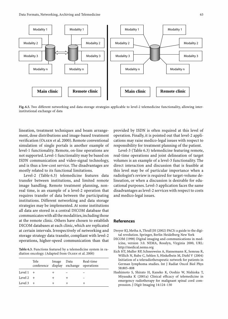
Data Formats, Networking, Archiving and Telemedicine 63

Table 6.3. Functions featured by a telemedicine system in ra-diation oncology. (Adapted from Olsen et al. 2000)

Tele conference

Image display

Data exchange

Real-time operations

Level 1 + + – –

Level 2 + + + –

Level 3 + + + +

lineation, treatment techniques and beam arrange-ment, dose distributions and image-based treatment verifi cation (Olsen et al. 2000). Remote conventional simulation of single portals is another example of level-1 functionality. Remote, on-line operations are not supported. Level-1 functionality may be based on ISDN communication and video-signal technology, and is thus a low-cost service. The disadvantages are mostly related to its functional limitations.

Level-2 (Table 6.3) telemedicine features data transfer between institutions, and limited remote image handling. Remote treatment planning, non-real time, is an example of a level-2 operation that requires transfer of data between the participating institutions. Different networking and data storage strategies may be implemented. At some institutions all data are stored in a central DICOM database that communicates with all the modalities, including those at the remote clinic. Others have chosen to establish DICOM databases at each clinic, which are replicated at certain intervals. Irrespectively of networking and storage strategy data transfer, compliant with level-2 operations, higher-speed communication than that

provided by ISDN is often required at this level of operation. Finally, it is pointed out that level-2 appli-cations may raise medico-legal issues with respect to responsibility for treatment planning of the patient.

Level-3 (Table 6.3) telemedicine featuring remote, real-time operations and joint delineation of target volumes is an example of a level-3 functionality. The direct interaction and discussion that is feasible at this level may be of particular importance when a radiologist’s review is required for target-volume de-lineation, or when a discussion is desirable for edu-cational purposes. Level-3 application faces the same disadvantages as level-2 services with respect to costs and medico-legal issues.

References

Dreyer KJ, Metha A, Thrall JH (2002) PACS: a guide to the digi-tal revolution. Springer, Berlin Heidelberg New York

DICOM (1998) Digital imaging and communications in med-icine, version 3.0. NEMA, Rosslyn, Virginia 2000, URL: http://medical.nema.org

Eich HT, Muller RP, Schneeweiss A, Hansemann K, Semrau R, Willich N, Rube C, Sehlen S, Hinkelbein M, Diehl V (2004) Initiation of a teleradiotherapeutic network for patients in German lymphoma studies. Int J Radiat Oncol Biol Phys 58:805–808

Hashimoto S, Shirato H, Kaneko K, Ooshio W, Nishioka T, Miyasaka K (2001a) Clinical effi cacy of telemedicine in emergency radiotherapy for malignant spinal cord com-pression. J Digit Imaging 14:124–130

Main clinic Remote clinic Main clinic Remote clinic

Fig. 6.5. Two different networking and data-storage strategies applicable to level-2 telemedicine functionality, allowing inter-institutional exchange of data

64 K. Eilertsen and D. R. Olsen

Hashimoto S, Shirato H, Nishioka T, Kagei K, Shimizu S, Fujita K, Ogasawara H, Watanabe Y, Miyasaka K (2001b) Remote verifi cation in radiotherapy using digitally reconstructed radiography (DRR) and portal images: a pilot study. Int J Radiat Oncol Biol Phys 50:579–585

Huh SJ, Shirato H, Hashimoto S, Shimizu S, Kim DY, Ahn YC, Choi D, Miyasaka K, Mizuno J (2000) An integrated service digital net-work (ISDN)-based international telecommunication between Samsung Medical Center and Hokkaido University using tele-communication helped radiotherapy planning and informa-tion system (THERAPIS). Radiother Oncol 56:121–123

Lemke HU (1991) The Berlin Communication System (BERKOM). In: Huang HK (ed) Picture Archiving and Com-munication Systems (PACS). Medicine, series F. Springer, Berlin Heidelberg New York (Computer and Systems Sci-ence, vol 74)

Ntasis E, Maniatis TA, Nikita KS (2003) Secure environment for real-time tele-collaboration on virtual simulation of radia-

tion treatment planning. Technol Health Care 11:41–52Olsen DR, Bruland S, Davis BJ (2000) Telemedicine in radio-

therapy treatment planning: requirements and applica-tions. Radiother Oncol 54:255–259

Purdy JA, Harms WB, Michalski J, Cox JD (1996) Multi-insti-tutional clinical trials: 3-D conformal radiotherapy qual-ity assurance. Guidelines in an NCI/RTOG study evaluat-ing dose escalation in prostate cancer radiotherapy. Front Radiat Ther Oncol 29:255–263

Reith A, Olsen DR, Bruland O, Bernder A, Risberg B (2003) Information technology in action: the example of Norway. Stud Health Technol Inform 96:186–189

Smith CL, Chu WK, Enke C (1998) A review of digital image networking technologies for radiation oncology treatment planning. Med Dosim 23:271–277

Stitt JA (1998) A system of tele-oncology at the University of Wisconsin Hospital and Clinics and regional oncology affi liate institutions. World Med J 97:38–42

Clinical X-Ray Computed Tomography 65

3D Imaging for Radiotherapy

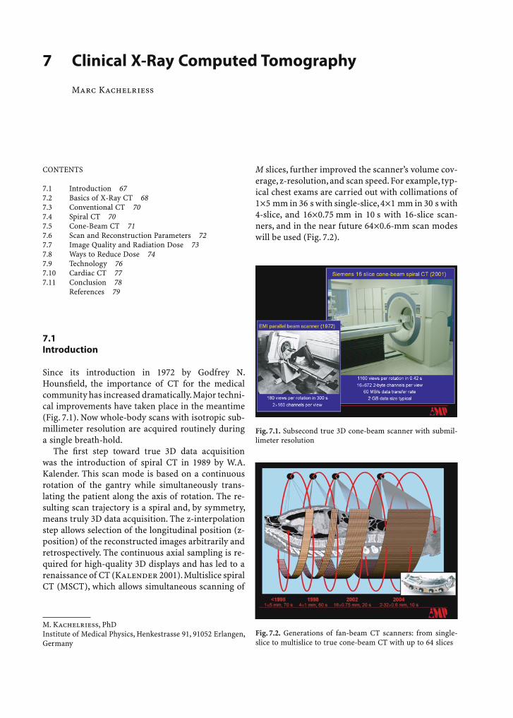
Clinical X-Ray Computed Tomography 67

7 Clinical X-Ray Computed Tomography

Marc Kachelriess

M. Kachelriess, PhDInstitute of Medical Physics, Henkestrasse 91, 91052 Erlangen, Germany

7.1 Introduction

Since its introduction in 1972 by Godfrey N. Hounsfi eld, the importance of CT for the medical community has increased dramatically. Major techni-cal improvements have taken place in the meantime (Fig. 7.1). Now whole-body scans with isotropic sub-millimeter resolution are acquired routinely during a single breath-hold.

The fi rst step toward true 3D data acquisition was the introduction of spiral CT in 1989 by W.A. Kalender. This scan mode is based on a continuous rotation of the gantry while simultaneously trans-lating the patient along the axis of rotation. The re-sulting scan trajectory is a spiral and, by symmetry, means truly 3D data acquisition. The z-interpolation step allows selection of the longitudinal position (z-position) of the reconstructed images arbitrarily and retrospectively. The continuous axial sampling is re-quired for high-quality 3D displays and has led to a renaissance of CT (Kalender 2001). Multislice spiral CT (MSCT), which allows simultaneous scanning of

M slices, further improved the scanner’s volume cov-erage, z-resolution, and scan speed. For example, typ-ical chest exams are carried out with collimations of 1¥5 mm in 36 s with single-slice, 4¥1 mm in 30 s with 4-slice, and 16¥0.75 mm in 10 s with 16-slice scan-ners, and in the near future 64¥0.6-mm scan modes will be used (Fig. 7.2).

CONTENTS

7.1 Introduction 677.2 Basics of X-Ray CT 687.3 Conventional CT 707.4 Spiral CT 707.5 Cone-Beam CT 717.6 Scan and Reconstruction Parameters 727.7 Image Quality and Radiation Dose 737.8 Ways to Reduce Dose 747.9 Technology 767.10 Cardiac CT 777.11 Conclusion 78 References 79

Fig. 7.2. Generations of fan-beam CT scanners: from single-slice to multislice to true cone-beam CT with up to 64 slices

Fig. 7.1. Subsecond true 3D cone-beam scanner with submil-limeter resolution

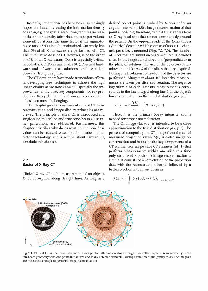
68 M. Kachelriess

Recently, patient dose has become an increasingly important issue: increasing the information density of a scan, e.g., the spatial resolution, requires increase of the photon density (absorbed photons per volume element) by at least the same factor if the signal-to-noise ratio (SNR) is to be maintained. Currently, less than 5% of all X-ray exams are performed with CT. The cumulative dose of CT, however, is of the order of 40% of all X-ray exams. Dose is especially critical in pediatric CT (Brenner et al. 2001). Practical hard-ware- and software-based solutions to reduce patient dose are strongly required.

The CT developers have made tremendous efforts in developing new techniques to achieve the high image quality as we now know it. Especially the im-provement of the three key components – X-ray pro-duction, X-ray detection, and image reconstruction – has been most challenging.

This chapter gives an overview of clinical CT. Basic reconstruction and image display principles are re-viewed. The principle of spiral CT is introduced and single-slice, multislice, and true cone-beam CT scan-ner generations are addressed. Furthermore, this chapter describes why doses went up and how dose values can be reduced. A section about tube and de-tector technology, and a section about cardiac CT, conclude this chapter.

7.2 Basics of X-Ray CT

Clinical X-ray CT is the measurement of an object’s X-ray absorption along straight lines. As long as a

desired object point is probed by X-rays under an angular interval of 180∞, image reconstruction of that point is possible; therefore, clinical CT scanners have an X-ray focal spot that rotates continuously around the patient. On the opposing side of the X-ray tube a cylindrical detector, which consists of about 103 chan-nels per slice, is mounted (Figs. 7.2, 7.3). The number of slices that are simultaneously acquired is denoted as M. In the longitudinal direction (perpendicular to the plane of rotation) the size of the detectors deter-mines the thickness S of the slices that are acquired. During a full rotation 103 readouts of the detector are performed. Altogether about 106 intensity measure-ments are taken per slice and rotation. The negative logarithm p of each intensity measurement I corre-sponds to the line integral along line L of the object’s linear attenuation coeffi cient distribution µ(x, y, z):

0

( )( ) ln ( , , )L

I Lp L dL x y zI

µ= − = ∫Here, I0 is the primary X-ray intensity and is

needed for proper normalization.The CT image ƒ(x, y, z) is intended to be a close

approximation to the true distribution µ(x, y, z). The process of computing the CT image from the set of measured projection values p(L) is called image re-construction and is one of the key components of a CT scanner. For single-slice CT scanners (M=1) that perform measurements within one slice at a time only (at a fi xed z-position) image reconstruction is simple. It consists of a convolution of the projection data with the reconstruction kernel followed by a backprojection into image domain:

cos sin0

( , ) ( , ) ( )x y

f x y d p kπ

ξ ϑ ϑϑ ϑ ξ ξ

= += ∗∫ .

Fig. 7.3. Clinical CT is the measurement of X-ray photon attenuation along straight lines. The in-plane scan geometry is the fan-beam geometry with one point-like source and many detector elements. During a rotation of the gantry many line integrals are measured, enough to perform image reconstruction

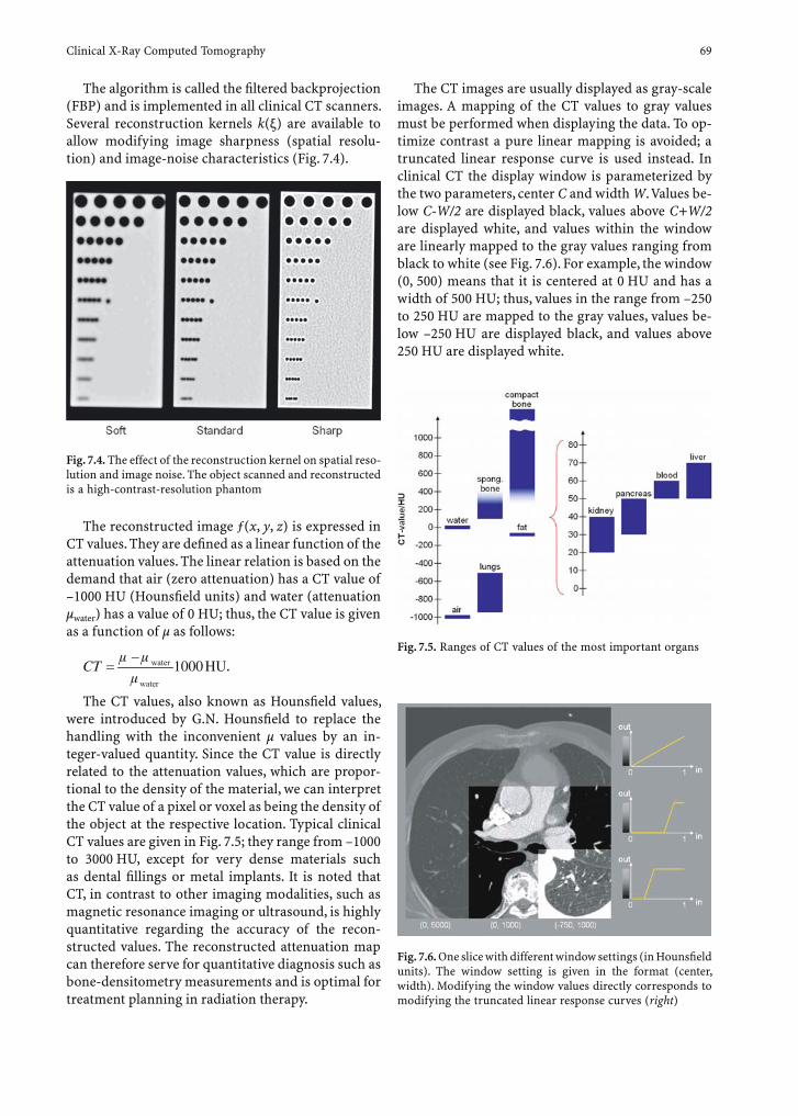
Clinical X-Ray Computed Tomography 69

The algorithm is called the fi ltered backprojection (FBP) and is implemented in all clinical CT scanners. Several reconstruction kernels k(x) are available to allow modifying image sharpness (spatial resolu-tion) and image-noise characteristics (Fig. 7.4).

The CT images are usually displayed as gray-scale images. A mapping of the CT values to gray values must be performed when displaying the data. To op-timize contrast a pure linear mapping is avoided; a truncated linear response curve is used instead. In clinical CT the display window is parameterized by the two parameters, center C and width W. Values be-low C-W/2 are displayed black, values above C+W/2 are displayed white, and values within the window are linearly mapped to the gray values ranging from black to white (see Fig. 7.6). For example, the window (0, 500) means that it is centered at 0 HU and has a width of 500 HU; thus, values in the range from –250 to 250 HU are mapped to the gray values, values be-low –250 HU are displayed black, and values above 250 HU are displayed white.

Fig. 7.4. The effect of the reconstruction kernel on spatial reso-lution and image noise. The object scanned and reconstructed is a high-contrast-resolution phantom

The reconstructed image ƒ(x, y, z) is expressed in CT values. They are defi ned as a linear function of the attenuation values. The linear relation is based on the demand that air (zero attenuation) has a CT value of –1000 HU (Hounsfi eld units) and water (attenuation µwater) has a value of 0 HU; thus, the CT value is given as a function of µ as follows:

water

water

1000HUCTµ µ

µ

−= .

The CT values, also known as Hounsfi eld values, were introduced by G.N. Hounsfi eld to replace the handling with the inconvenient µ values by an in-teger-valued quantity. Since the CT value is directly related to the attenuation values, which are propor-tional to the density of the material, we can interpret the CT value of a pixel or voxel as being the density of the object at the respective location. Typical clinical CT values are given in Fig. 7.5; they range from –1000 to 3000 HU, except for very dense materials such as dental fi llings or metal implants. It is noted that CT, in contrast to other imaging modalities, such as magnetic resonance imaging or ultrasound, is highly quantitative regarding the accuracy of the recon-structed values. The reconstructed attenuation map can therefore serve for quantitative diagnosis such as bone-densitometry measurements and is optimal for treatment planning in radiation therapy.

Fig. 7.6. One slice with different window settings (in Hounsfi eld units). The window setting is given in the format (center, width). Modifying the window values directly corresponds to modifying the truncated linear response curves (right)

Fig. 7.5. Ranges of CT values of the most important organs

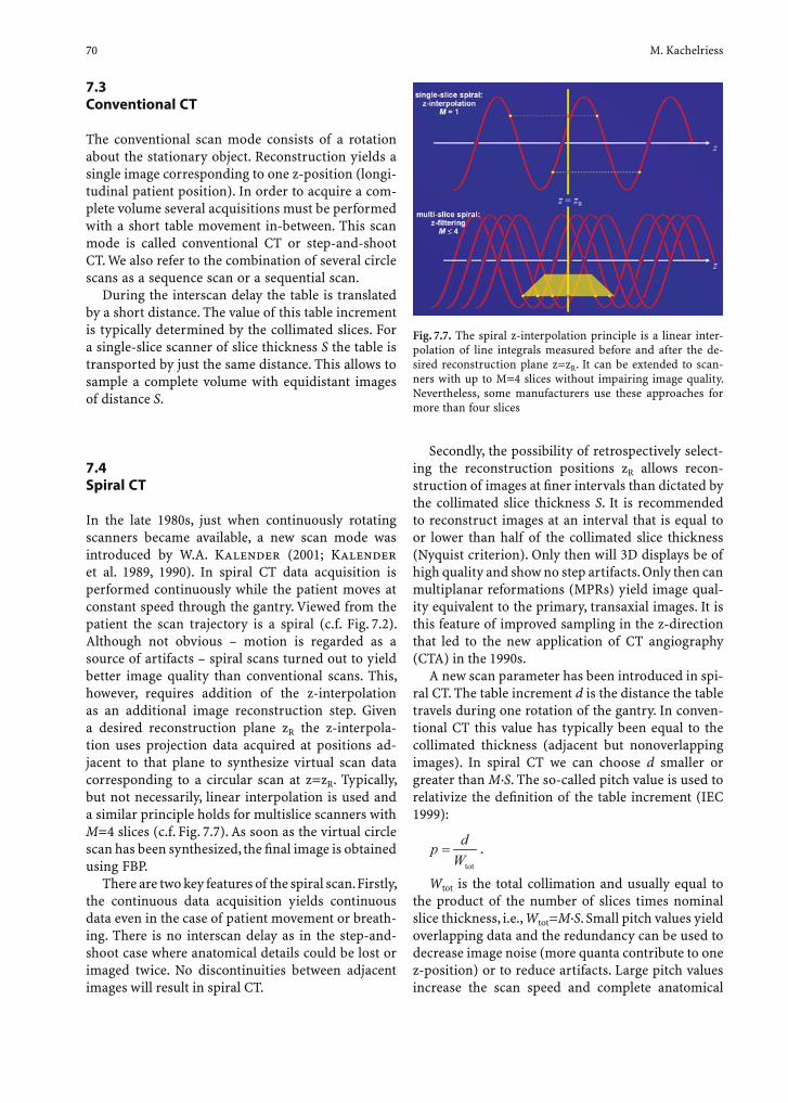
70 M. Kachelriess

7.3 Conventional CT

The conventional scan mode consists of a rotation about the stationary object. Reconstruction yields a single image corresponding to one z-position (longi-tudinal patient position). In order to acquire a com-plete volume several acquisitions must be performed with a short table movement in-between. This scan mode is called conventional CT or step-and-shoot CT. We also refer to the combination of several circle scans as a sequence scan or a sequential scan.

During the interscan delay the table is translated by a short distance. The value of this table increment is typically determined by the collimated slices. For a single-slice scanner of slice thickness S the table is transported by just the same distance. This allows to sample a complete volume with equidistant images of distance S.

7.4 Spiral CT

In the late 1980s, just when continuously rotating scanners became available, a new scan mode was introduced by W.A. Kalender (2001; Kalender et al. 1989, 1990). In spiral CT data acquisition is performed continuously while the patient moves at constant speed through the gantry. Viewed from the patient the scan trajectory is a spiral (c.f. Fig. 7.2). Although not obvious – motion is regarded as a source of artifacts – spiral scans turned out to yield better image quality than conventional scans. This, however, requires addition of the z-interpolation as an additional image reconstruction step. Given a desired reconstruction plane zR the z-interpola-tion uses projection data acquired at positions ad-jacent to that plane to synthesize virtual scan data corresponding to a circular scan at z=zR. Typically, but not necessarily, linear interpolation is used and a similar principle holds for multislice scanners with M=4 slices (c.f. Fig. 7.7). As soon as the virtual circle scan has been synthesized, the fi nal image is obtained using FBP.

There are two key features of the spiral scan. Firstly, the continuous data acquisition yields continuous data even in the case of patient movement or breath-ing. There is no interscan delay as in the step-and-shoot case where anatomical details could be lost or imaged twice. No discontinuities between adjacent images will result in spiral CT.

Secondly, the possibility of retrospectively select-ing the reconstruction positions zR allows recon-struction of images at fi ner intervals than dictated by the collimated slice thickness S. It is recommended to reconstruct images at an interval that is equal to or lower than half of the collimated slice thickness (Nyquist criterion). Only then will 3D displays be of high quality and show no step artifacts. Only then can multiplanar reformations (MPRs) yield image qual-ity equivalent to the primary, transaxial images. It is this feature of improved sampling in the z-direction that led to the new application of CT angiography (CTA) in the 1990s.

A new scan parameter has been introduced in spi-ral CT. The table increment d is the distance the table travels during one rotation of the gantry. In conven-tional CT this value has typically been equal to the collimated thickness (adjacent but nonoverlapping images). In spiral CT we can choose d smaller or greater than M·S. The so-called pitch value is used to relativize the defi nition of the table increment (IEC 1999):

tot

dpW

=

.

Wtot is the total collimation and usually equal to the product of the number of slices times nominal slice thickness, i.e., Wtot=M·S. Small pitch values yield overlapping data and the redundancy can be used to decrease image noise (more quanta contribute to one z-position) or to reduce artifacts. Large pitch values increase the scan speed and complete anatomical

Fig. 7.7. The spiral z-interpolation principle is a linear inter-polation of line integrals measured before and after the de-sired reconstruction plane z=zR. It can be extended to scan-ners with up to M=4 slices without impairing image quality. Nevertheless, some manufacturers use these approaches for more than four slices

Clinical X-Ray Computed Tomography 71

ranges can be covered very fast. Typical values are between 0.3 and 1.5. For single-slice scanners pitch values up to 2 are allowed.

7.5 Cone-Beam CT

Recently, scanners that simultaneously acquire more than one slice have become available. The run for more slices started in 1998 with the introduction of four-slice scanners.1 The advantages of scan-ning more than one slice are obvious. For a given range scan time can be reduced by a factor of M. Alternatively, spatial resolution can be increased by the same factor. In fact, the typical scan modes were a combination of both options and are illustrated in Fig. 7.2. Curiously, many sites switched from the 1×5 mm collimation to the 4×1 mm collimation and improvements in spatial resolution often seemed more important than improvements in scan time.

The most challenging component of cone-beam CT is the image reconstruction algorithm. In contrast to single-slice or four-slice scanners, where each ac-quired slice can be regarded as being (approximately) perpendicular to the axis of rotation (c.f. Fig. 7.7), the cone-beam nature in scanners with many slices must not be neglected. Two object points located at the same z- but at different x- or y-positions will con-tribute to different slices (Fig. 7.8); hence, image re-construction must take the cone-angle explicitly into account, now.

Two dedicated cone-beam algorithms are imple-mented in the product software of the present clini-cal 16- to 64-slice CT scanners: adapted versions of the Feldkamp algorithm and modifi cations of the ad-vanced single-slice rebinning (ASSR) algorithm.

The Feldkamp algorithm is an extension of the 2D reconstruction to three dimensions (Feldkamp et al. 1984). It also consists of the convolution of the acquired data followed by a backprojection. In con-trast to the 2D case, the backprojection is 3D for the Feldkamp algorithm and during image reconstruc-tion a complete volume must be kept in memory (Fig. 7.9).

The ASSR uses the fact that 180∞ segments of circles can be accurately fi tted to the spiral trajectory as long as tilting of these circles with respect to the x–y plane is allowed (Kachelriess et al. 2000a). The ASSR re-sorts the acquired cone-beam data to correspond to virtual 2D scans along these tilted circles. Then, a standard 2D image reconstruction is performed on these reconstruction planes to obtain tilted im-ages. The ASSR uses many adjacent and overlapping reconstruction planes to suffi ciently cover the whole volume. As soon as enough tilted images are avail-able, the data are resampled in spatial domain to ob-

1 Before 1998 some scanners, such as the EMI scanner, the Siemens SIRETOM, the Imatron C-100, and the Elscint Twin scanner, were able to acquire two slices simultaneously. The detector and image reconstruction technology used, how-ever, did not allow to further increase the number of slices towards true cone-beam scans.

Fig. 7.8. The longitudinal cut illustrates the cone-beam prob-lem. For scanners with many slices (M>4) it is prohibitive, with respect to image quality, to reconstruct the slices sepa-rately. The demand for cone-beam reconstruction algorithms has led to new approaches in CT image reconstruction

Fig. 7.9. Basic principles of advanced single-slice rebinning (ASSR)-type and Feldkamp-type reconstruction

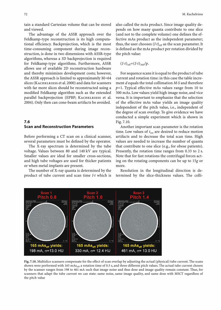
72 M. Kachelriess

tain a standard Cartesian volume that can be stored and viewed.

The advantage of the ASSR approach over the Feldkamp-type reconstruction is its high computa-tional effi ciency. Backprojection, which is the most time-consuming component during image recon-struction, is done in two dimensions with ASSR-type algorithms, whereas a 3D backprojection is required for Feldkamp-type algorithms. Furthermore, ASSR allows use of available 2D reconstruction hardware and thereby minimizes development costs; however, the ASSR approach is limited to approximately M=64 slices (Kachelriess et al. 2000) and data for scanners with far more slices should be reconstructed using a modifi ed Feldkamp algorithm such as the extended parallel backprojection (EPBP; Kachelriess et al. 2004). Only then can cone-beam artifacts be avoided.

7.6 Scan and Reconstruction Parameters

Before performing a CT scan on a clinical scanner, several parameters must be defi ned by the operator.

The X-ray spectrum is determined by the tube voltage. Values between 80 and 140 kV are typical. Smaller values are ideal for smaller cross-sections, and high tube voltages are used for thicker patients or when metal implants are present.

The number of X-ray quanta is determined by the product of tube current and scan time I·t which is

also called the mAs product. Since image quality de-pends on how many quanta contribute to one slice (and not to the complete volume) one defi nes the ef-fective mAs product as the independent parameter; thus, the user chooses (I·t)eff as the scan parameter. It is defi ned as the mAs product per rotation divided by the pitch value:

(I·t)eff=(I·t)360 /p.

For sequence scans it is equal to the product of tube current and rotation time: in this case the table incre-ment d equals the total collimation M·S and therefore p=1. Typical effective mAs values range from 10 to 500 mAs. Low values yield high image noise, and vice versa. It is important to emphasize that the selection of the effective mAs value yields an image quality independent of the pitch value, i.e., independent of the degree of scan overlap. To give evidence we have conducted a simple experiment which is shown in Fig. 7.10.

Another important scan parameter is the rotation time. Low values of trot are desired to reduce motion artifacts and to decrease the total scan time. High values are needed to increase the number of quanta that contribute to one slice (e.g., for obese patients). Presently, the rotation time ranges from 0.33 to 2 s. Note that for fast rotations the centrifugal forces act-ing on the rotating components can be up to 15g or more.

Resolution in the longitudinal direction is de-termined by the slice-thickness values. The colli-

Fig. 7.10. Multislice scanners compensate for the effect of scan overlap by adjusting the actual (physical) tube current. The scans shown were performed with 165 mAseff, a rotation time of 0.5 s, and three different pitch values. The actual tube current chosen by the scanner ranges from 198 to 461 mA such that image noise and thus dose and image quality remain constant. Thus, for scanners that adapt the tube current we can state: same noise, same image quality, and same dose with MSCT regardless of the pitch value

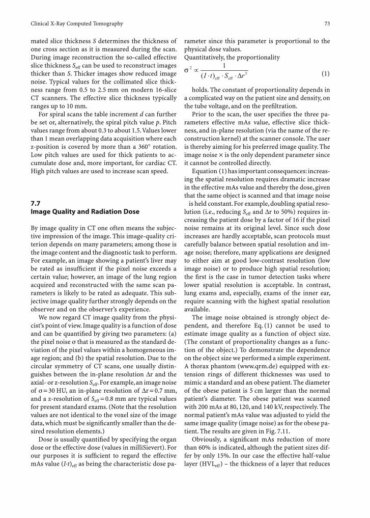
Clinical X-Ray Computed Tomography 73

mated slice thickness S determines the thickness of one cross section as it is measured during the scan. During image reconstruction the so-called effective slice thickness Seff can be used to reconstruct images thicker than S. Thicker images show reduced image noise. Typical values for the collimated slice thick-ness range from 0.5 to 2.5 mm on modern 16-slice CT scanners. The effective slice thickness typically ranges up to 10 mm.

For spiral scans the table increment d can further be set or, alternatively, the spiral pitch value p. Pitch values range from about 0.3 to about 1.5. Values lower than 1 mean overlapping data acquisition where each z-position is covered by more than a 360∞ rotation. Low pitch values are used for thick patients to ac-cumulate dose and, more important, for cardiac CT. High pitch values are used to increase scan speed.

7.7 Image Quality and Radiation Dose

By image quality in CT one often means the subjec-tive impression of the image. This image-quality cri-terion depends on many parameters; among those is the image content and the diagnostic task to perform. For example, an image showing a patient’s liver may be rated as insuffi cient if the pixel noise exceeds a certain value; however, an image of the lung region acquired and reconstructed with the same scan pa-rameters is likely to be rated as adequate. This sub-jective image quality further strongly depends on the observer and on the observer’s experience.

We now regard CT image quality from the physi-cist’s point of view. Image quality is a function of dose and can be quantifi ed by giving two parameters: (a) the pixel noise s that is measured as the standard de-viation of the pixel values within a homogeneous im-age region; and (b) the spatial resolution. Due to the circular symmetry of CT scans, one usually distin-guishes between the in-plane resolution ∆r and the axial- or z-resolution Seff. For example, an image noise of s = 30 HU, an in-plane resolution of ∆r = 0.7 mm, and a z-resolution of Seff = 0.8 mm are typical values for present standard exams. (Note that the resolution values are not identical to the voxel size of the image data, which must be signifi cantly smaller than the de-sired resolution elements.)

Dose is usually quantifi ed by specifying the organ dose or the effective dose (values in milliSievert). For our purposes it is suffi cient to regard the effective mAs value (I·t)eff as being the characteristic dose pa-

rameter since this parameter is proportional to the physical dose values.Quantitatively, the proportionality

23

eff eff

1( )I t S r

σ ∝⋅ ⋅ ⋅∆ (1)

holds. The constant of proportionality depends in a complicated way on the patient size and density, on the tube voltage, and on the prefi ltration.

Prior to the scan, the user specifi es the three pa-rameters effective mAs value, effective slice thick-ness, and in-plane resolution (via the name of the re-construction kernel) at the scanner console. The user is thereby aiming for his preferred image quality. The image noise ¥ is the only dependent parameter since it cannot be controlled directly.

Equation (1) has important consequences: increas-ing the spatial resolution requires dramatic increase in the effective mAs value and thereby the dose, given that the same object is scanned and that image noise

is held constant. For example, doubling spatial reso-lution (i.e., reducing Seff and ∆r to 50%) requires in-creasing the patient dose by a factor of 16 if the pixel noise remains at its original level. Since such dose increases are hardly acceptable, scan protocols must carefully balance between spatial resolution and im-age noise; therefore, many applications are designed to either aim at good low-contrast resolution (low image noise) or to produce high spatial resolution; the fi rst is the case in tumor detection tasks where lower spatial resolution is acceptable. In contrast, lung exams and, especially, exams of the inner ear, require scanning with the highest spatial resolution available.

The image noise obtained is strongly object de-pendent, and therefore Eq. (1) cannot be used to estimate image quality as a function of object size. (The constant of proportionality changes as a func-tion of the object.) To demonstrate the dependence on the object size we performed a simple experiment. A thorax phantom (www.qrm.de) equipped with ex-tension rings of different thicknesses was used to mimic a standard and an obese patient. The diameter of the obese patient is 5 cm larger than the normal patient’s diameter. The obese patient was scanned with 200 mAs at 80, 120, and 140 kV, respectively. The normal patient’s mAs value was adjusted to yield the same image quality (image noise) as for the obese pa-tient. The results are given in Fig. 7.11.

Obviously, a signifi cant mAs reduction of more than 60% is indicated, although the patient sizes dif-fer by only 15%. In our case the effective half-value layer (HVLeff) – the thickness of a layer that reduces

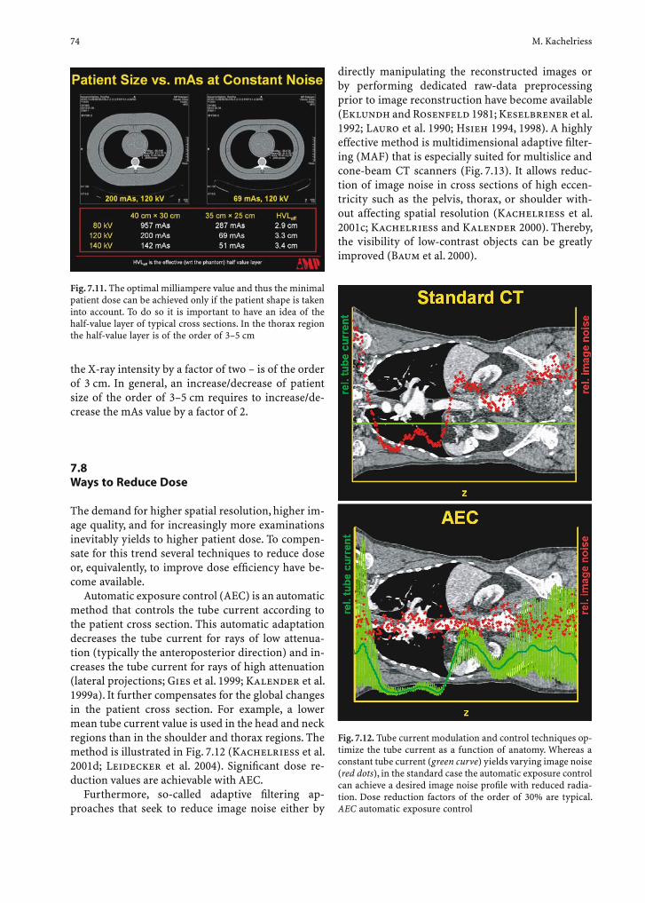
74 M. Kachelriess

the X-ray intensity by a factor of two – is of the order of 3 cm. In general, an increase/decrease of patient size of the order of 3–5 cm requires to increase/de-crease the mAs value by a factor of 2.

7.8 Ways to Reduce Dose

The demand for higher spatial resolution, higher im-age quality, and for increasingly more examinations inevitably yields to higher patient dose. To compen-sate for this trend several techniques to reduce dose or, equivalently, to improve dose effi ciency have be-come available.

Automatic exposure control (AEC) is an automatic method that controls the tube current according to the patient cross section. This automatic adaptation decreases the tube current for rays of low attenua-tion (typically the anteroposterior direction) and in-creases the tube current for rays of high attenuation (lateral projections; Gies et al. 1999; Kalender et al. 1999a). It further compensates for the global changes in the patient cross section. For example, a lower mean tube current value is used in the head and neck regions than in the shoulder and thorax regions. The method is illustrated in Fig. 7.12 (Kachelriess et al. 2001d; Leidecker et al. 2004). Signifi cant dose re-duction values are achievable with AEC.

Furthermore, so-called adaptive fi ltering ap-proaches that seek to reduce image noise either by

Fig. 7.11. The optimal milliampere value and thus the minimal patient dose can be achieved only if the patient shape is taken into account. To do so it is important to have an idea of the half-value layer of typical cross sections. In the thorax region the half-value layer is of the order of 3–5 cm

Fig. 7.12. Tube current modulation and control techniques op-timize the tube current as a function of anatomy. Whereas a constant tube current (green curve) yields varying image noise (red dots), in the standard case the automatic exposure control can achieve a desired image noise profi le with reduced radia-tion. Dose reduction factors of the order of 30% are typical. AEC automatic exposure control

directly manipulating the reconstructed images or by performing dedicated raw-data preprocessing prior to image reconstruction have become available (Eklundh and Rosenfeld 1981; Keselbrener et al. 1992; Lauro et al. 1990; Hsieh 1994, 1998). A highly effective method is multidimensional adaptive fi lter-ing (MAF) that is especially suited for multislice and cone-beam CT scanners (Fig. 7.13). It allows reduc-tion of image noise in cross sections of high eccen-tricity such as the pelvis, thorax, or shoulder with-out affecting spatial resolution (Kachelriess et al. 2001c; Kachelriess and Kalender 2000). Thereby, the visibility of low-contrast objects can be greatly improved (Baum et al. 2000).

Clinical X-Ray Computed Tomography 75

The largest dose reduction potential, however, lies in scan protocol optimization. Especially the param-eters scan length and effective mAs value lend them-selves to optimization. Often the scan length exceeds the anatomical region of interest by 5 or even 10 cm. For short organs (e.g., the heart has a longitudinal ex-tension of about 15 cm) this can mean a waste of dose. Whereas this parameter can be minimized easily, the optimization of the tube current is very diffi cult since it depends on many parameters, as we have seen. Only

highly experienced operators can minimize the mAs value and still obtain images of suffi cient diagnostic values. To experience the effect of mAs optimization one can use the dose tutor software (www.vamp-gmbh.de). It uses acquired raw data and adds virtual noise to each projection value to convert the data to a lower mAs value. This tool helps to iteratively seek for the optimal scan parameters and to learn more about the relationship between patient shape and im-age noise (Fig. 7.14).

Fig. 7.13. Multidimensional adaptive fi ltering signifi cantly reduces image noise and correlated noise structure (streaks). The subtraction image shows that there is no loss in resolution

Fig. 7.14. Dose tutoring also means experiencing the dependence of image quality as a function of milliampere value. Software tools, such as the dose tutor shown here, allow manipulation of the milliampere value retrospectively by adding noise to the raw data

76 M. Kachelriess

Individual dose assessment will play a signifi cant role in the future. For example, the European Union Directive (European Communities 1997) demands the specifi cation of the individual patient dose for every CT examination. To directly assess scanner- and organ-specifi c dose values, dose calculators have become available. Based on Monte Carlo dose calcu-lations (Schmidt and Kalender 2002) they allow computation of organ dose and effective dose values as a function of the scanner type and scan proto-col (Fig. 7.15). The effective dose is regarded as the best indicator of stochastic risk such as induction of malignancy. It expresses the summed dose value over all organs weighted by their radiation sensitivi-ties. The weighting factors are recommended by the International Commission on Radiation Protection (ICRP) (ICRP 1990).

Putting all the dose-reduction efforts, including dose training and dose information, together it is likely that the increase in patient dose will be lower than predicted by Eq. (1), although spatial resolution and image quality will improve.

pace with the increased scan speed. Even with mod-ern computing, power algorithms must be carefully designed and implemented. Two reconstructed slices per second (frames per second) are the minimum ac-ceptable reconstruction speed on modern scanners. Since a complete anatomic volume of, for example, 50 cm length and 0.6 mm resolution can be covered in less than 15 s of the order of several hundred to 1000 images must be reconstructed. Manufacturers use highly parallelized hardware to face this task.

The drastic increase in scan speed demands the same increase in tube power since the same number of photons must be provided in a shorter time. To ensure high patient throughput cooling delays must be reduced in the same order. The drastic increase in rotation speed – rotation times of 0.4 s per rotation are typical presently and will certainly go down in the near future – is demanding with respect to the cen-trifugal forces that affect the tube housing and bear-ings. A typical tube is located 60 cm off the rotation axis. With 0.4 s per rotation, the resulting forces are of the order of 15g.

A typical X-ray tube consists of a vacuum-fi lled tube envelope. Inside the vacuum is the cathode and a rotating anode with one bearing (Fig. 7.16). This conventional concept has the disadvantage that tube cooling is not very effi cient and that the one-sided bearing cannot tolerate high forces. Further on, it is diffi cult to lubricate bearings in vacuum. To improve these conventional tubes vendors try to maximize the heat capacity (expressed in mega heat-units MHU) to protract cooling delays as long as possible. Recently, a new CT tube has become available where the cathode, the anode, and the envelope together rotate in the cooling medium (Fig. 7.16). Due to the direct contact to the cooling oil, there is no need for storing the heat and there will be no cooling delays.

X-ray photon detection in modern CT scanners is performed using a scintillator layer that converts the X-rays into visible light.2 Photodiodes convert the light to an electrical current that is amplifi ed and digitized. As soon as the number of detector rows exceeds 2, the arrangement of the electronic compo-nents that read out, amplify, and digitize the signal becomes nontrivial and increasingly diffi cult with in-creasingly more detector rows. Another challenging, and often limiting, aspect of multislice detector tech-nology is the data rates that must be transferred from

Fig. 7.15. Dose calculators compute organ-dose values and the weighted effective dose as a function of the anatomical region scanned and the scan parameters. (From www.vamp-gmbh.de; Kalender et al. 1999b)

7.9 Technology

The decisive technological steps towards multislice and cone-beam scanning are image reconstruction as well as tube and detector technology. Image re-construction techniques are demanding not only because the cone-beam problem poses a mathemati-cally completely different situation than 2D scanning, but also because reconstruction speed must keep

2 The previous Xenon gas-chamber technology does not lend itself to dense packing and is not used in multislice scan-ners.

Clinical X-Ray Computed Tomography 77

the gantry to the acquisition computer. If we assume a rotation time of 0.4 s and let the scanner simultane-ously acquire 16 slices each of 800 two-byte channels per projection, with about 1000 projections per rota-tion a data transfer rate of 64 MB/s is required.

Due to these challenges, the present detectors typi-cally have more detector rows than can be read out simultaneously. Electronic combination (binning) of neighboring rows is used to generate thicker col-limated slices and to make use of all detector rows available. (Note that 16-slice CT scanners turned out to either have 24 or 32 detector rows, but none of them allow to simultaneously acquire more than 16 slices.) The 32-row scanners are of matrix-array type and combine every other row to generate thicker slices. The 24-row scanners are of adaptive array type and use thicker rows for the outermost slices. The adap-tive array technology has a higher X-ray sensitivity and requires less patient dose than the matrix array detectors. Illustrations of these concepts are given in Figs. 7.17 and 7.18.

7.10 Cardiac CT

One of the most prominent special applications at present is retrospectively gated CT of the heart. Improvements in CT technology, such as the intro-duction of spiral CT, subsecond rotation times, and multislice data acquisition, have stimulated cardiac CT imaging within the past decade. Cardiac spiral CT started with the introduction of dedicated phase-cor-related reconstruction algorithms for single-slice spi-ral CT in 1997 (Kachelriess and Kalender 1997,

Fig. 7.18. Detector concepts announced for 2004. Three of four manufacturers will provide adaptive array detectors to maxi-mize dose effi ciency for thicker slices. GE’s announcement of its 64-row detector remained unclear with respect to the maximum number of simultaneous acquired slices. It may be restricted to reading out M=32 slices and all 64 rows would only be needed after pair-wise binning. The Siemens detector provides only 32 high resolution detector rows but generates 64 high-resolution slices due to a fl ying focal spot that samples each row twice. Thereby it is the only detector that fulfi ls the Nyquist sampling criterion in the z-direction

Fig. 7.16. Conventional tubes have stationary envelope and sta-tionary cathode. Recently, high-performance tubes have become available that have a rotating envelope and therefore allow for direct cooling of the anode

Fig. 7.17. Photo of a 64-slice adaptive array detector. (Data cour-tesy of Siemens Medical Solutions, Forchheim, Germany)

78 M. Kachelriess

1998; Kachelriess et al. 1998). These approaches have been generalized to the case of multislice spiral CT (MSCT) acquisition (Kachelriess et al. 1998, 2000b; Taguchi and Anno 2000; Flohr et al. 2000) to process data of four-slice scanners. Since then, the algorithms have been extended to the case of cone-beam scanning with 16 slices (Kachelriess et al. 2001a,b; Kachelriess and Kalender 2002; Sourbelle et al. 2002) and to scanners with far more than 16 slices. Vendor-specifi c implementations that take into account the cone angle have not yet been published.The underlying principle of phase correlation is com-mon to all algorithms and is illustrated in Fig. 7.19. Highly overlapping spiral data (small pitch value) are acquired. In addition, a synchronization signal is either measured (ECG) [29] or calculated directly from the raw data (Kymogram; Kachelriess et al. 2002). The data redundancy obtained from the high overlap is then used to carefully select those data ranges that correspond to the desired motion phase of the heart for reconstruction. This yields image data with signifi cantly reduced motion artifacts but slightly increased image noise.

Retrospectively phase-correlated image recon-struction achieves high-quality images of the heart – especially in combination with multislice CT scan-ners and thin slice thicknesses. The cardiac images are typically used to either perform an automated quantifi cation of coronary calcium or to perform a CT angiography of the coronary arteries (Fig. 7.20).

7.11 Conclusion

Clinical X-ray CT has drastically improved over the past decades. Presently, multislice scanners with 16

submillimeter slices are routinely available and pro-vide highly accurate insight into the human anat-omy (Fig. 7.21). Isotropic spatial resolution values of 0.7 mm and less are typical for modern scanners. Scan times of the order of 15 s are suffi cient to scan complete anatomical regions within a single breath-hold. Rotation times of below 0.4 s per rotation in combination with phase-correlated image recon-struction algorithms allow obtainment of superb images of the human heart.

There is an ongoing demand for higher spatial resolution and faster scans. Manufacturers will pro-vide respective solutions (e.g., 64-slice scanners). To counteract the dose increase, hardware solutions (AEC) and algorithmic solutions (adaptive fi ltering) are being provided, too.

Fig. 7.19. Principle of retrospectively gated cardiac CT. One or more data segments are combined to yield a complete 180° data range with maximum temporal resolution.

Fig. 7.20. Routine examinations now achieve extremely high image quality. This image is a scan of the human heart with a high-speed multislice CT scanner and a rotating envelope tube. (Data courtesy of D. Ropers, Erlangen, Germany)

Clinical X-Ray Computed Tomography 79

References

Baum U, Lell M, Kachelriess M, Greess H, Kalender WA, Bautz WA (2000) Rawdata-based 3D adaptive fi ltering for CT scans of the cervicothoracic region: clinical evaluation. Radiology 217:413

Brenner DJ, Elliston CD, Hall EJ, Berdon WE (2001) Estimated risks of radiation induced fatal cancer from pediatric CT. Am J Roentgenol 176:289–296

Eklundh JO, Rosenfeld A (1981) Imaging smoothing based on neighbor linking. IEEE Trans Pattern Anal Mach Intell 3:679–683

European Communities (1997) Council Directive 97/43/Eura-tom of 30 June 1997 on health protection of individuals against the dangers of ionising radiation in relation to medical exposure, and repealing Directive 84/466/Euratom. Offi cial J Eur Comm no. L 180/22

Feldkamp LA, Davis LC, Kress JW (1984) Practical cone-beam algorithm. J Opt Soc Am 1:612–619

Flohr T, Ohnesorge B, Kopp AF, Becker C, Halliburton SS, Knez A (2000) A reconstruction concept for ECG-gated multi-slice spiral CT of the heart with pulse-rate adaptive

optimization of spatial and temporal resolution. Radiology 217:438

Gies M, Kalender WA, Wolf H, Suess C, Madsen MT (1999) Dose reduction in CT by anatomically adapted tube current modulation. I. Simulation studies. Med Phys 26:2235–2247

Hsieh J (1994) Generalized adaptive median fi lter and their application in computed tomography. SPIE Proc 2298:662–672

Hsieh J (1998) Adaptive streak artifact reduction in computed tomography resulting from excessive X-ray photon noise. Med Phys 25:2139–2147

ICRP (1990) (International Commission on Radiological Pro-tection) Publication 60. Recommendations of the Interna-tional Commission on Radiological Protection. Pergamon Press, Oxford

IEC (1999) International Electrotechnical Commission, 60601-2-44: medical electrical equipment, part 2-44. Particular requirements for the safety of X-ray equipment for com-puted tomography, Geneva, Switzerland

Kachelriess M, Kalender WA (1997) ECG-based phase-ori-ented reconstruction from subsecond spiral CT scans of the heart. Radiology 205:215

Fig. 7.21. Routine data acquired on a 16-slice CT scanner. Not only the quality of the CT images themselves but also the display techniques have been improved. Here, so-called volume renderings are shown. (Data courtesy of the Department of Diagnostic Radiology, Institute of Medical Physics, Erlangen, Germany)

80 M. Kachelriess

Kachelriess M, Kalender WA (1998) Electrocardiogram-corre-lated image reconstruction from subsecond spiral CT scans of the heart. Med Phys 25:2417–2431

Kachelriess M, Kalender WA (2000) Computertomograph mit reduzierter Dosisbelastung bzw. reduziertem Bildpunk-trauschen. Deutsches Patent- und Markenamt. Germany. Patent specifi cation DE 198 53 143

Kachelriess M, Kalender WA (2002) Extended parallel back-projection for cardiac cone-beam CT for up to 128 slices. Radiology 225:310

Kachelriess M, Kalender WA, Karakaya S, Achenbach S, Nossen J, Moshage W, et al. (1998) Imaging of the heart by ECG-oriented reconstruction from subsecond spiral CT scans. In: Glazer G, Krestin G (eds) Advances in CT IV. Springer, Berlin Heidelberg New York, pp 137–143

Kachelriess M, Schaller S, Kalender WA (2000a) Advanced single-slice rebinning in cone-beam spiral CT. Med Phys 27:754–772

Kachelriess M, Ulzheimer S, Kalender WA (2000b) ECG-corre-lated imaging of the heart with subsecond multi-slice spiral CT. IEEE Trans Med Imaging (Spec Issue) 19:888–901

Kachelriess M, Fuchs T, Lapp R, Sennst D-A, Schaller S, Kal-ender WA (2001a) Image to volume weighting generalized ASSR for arbitrary pitch 3D and phase-correlated 4D spiral cone-beam CT reconstruction. Proc 2001 International Meeting on Fully 3D Image Reconstruction, Pacifi c Grove, Calif., pp 179–182

Kachelriess M, Watzke O, Kalender WA (2001b) Generalized multi-dimensional adaptive fi ltering for conventional and spiral single-slice, multi-slice, and cone-beam CT. Med Phys 28:475–490

Kachelriess M, Sennst D-A, Kalender WA (2001c) 4D phase-correlated spiral cardiac reconstruction using image to volume weighting generalized ASSR for a 16-slice cone-beam CT. Radiology 221:457

Kachelriess M, Leidecker C, Kalender WA (2001d) Image qual-ity-oriented automatic exposure control (iqAEC) for spiral CT. Radiology 221:366

Kachelriess M, Sennst D-A, Maxlmoser W, Kalender WA (2002)

Kymogram detection and kymogram-correlated image reconstruction from sub-second spiral computed tomog-raphy scans of the heart. Med Phys 29 : 1489–1503

Kachelriess M, Knaup M, Kalender WA (2004) Extended par-allel backprojection for standard 3D and phase-selective 4D axial and spiral cone-beam CT with arbitrary pitch and dose usage. Med Phys 31:1623–1641

Kalender WA (2001) Computed tomography. Wiley, New YorkKalender WA, Seissler W, Vock P (1989) Single-breath-hold

spiral volumetric CT by continuous patient translation and scanner rotation. Radiology 173:414

Kalender WA, Seissler W, Klotz E, Vock P (1990) Spiral volu-metric CT with single-breath-hold technique, continuous transport, and continuous scanner rotation. Radiology 176:181–183

Kalender WA, Wolf H, Suess C (1999a) Dose reduction in CT by anatomically adapted tube current modulation II. Phantom measurements. Med Phys 26:2248–2253

Kalender WA, Schmidt B, Zankl M, Schmidt M (1999b) A PC program for estimating organ dose and effective dose values in computed tomography. Eur Radiol 9:555–562

Keselbrener L, Shimoni Y, Akselrod S (1992) Nonlinear fi lters applied on computerized axial tomography. Theory and phantom images. Med Phys 19:1057–1064

Lauro KL, Heuscher DJ, Kesavan H (1990) Bandwidth fi ltering of CT scans of the spine. Radiology 177:307

Leidecker C, Kachelriess M, Kalender WA (2004) Comparison of an attenuation-based automatic exposure control (AEC) to alternative methods utilizing localizer radiographs. Eur Radiol 14 (Suppl 2):247

Schmidt B, Kalender WA (2002) A fast voxel-based Monte Carlo method for scanner- and patient-specifi c dose calculations in computed tomography. Phys Med XVIII:43–53

Sourbelle K, Kachelriess M, Kalender WA (2002) Feldkamp-type reconstruction algorithm for spiral cone-beam (CB) computed tomography (CT). Radiology 225:451

Taguchi K, Anno H (2000) High temporal resolution for mul-tislice helical computed tomography. Med Phys 27:861–872

4D Imaging and Treatment Planning 81

8 4D Imaging and Treatment Planning

Eike Rietzel and George T.Y. Chen

E. Rietzel, MDSiemens Medical Solutions, Particle Therapy, Henkestrasse 127, 91052 Erlangen, GermanyG. T. Y. Chen, MDDepartment of Radiation Oncology, Massachusetts General Hospital, 30 Fruit Street, Boston, MA 02114, USA

8.1 Introduction

Respiratory motion can introduce signifi cant errors in radiotherapy imaging, treatment planning, and treatment delivery (Balter et al. 1996; Chen et al. 2004; Shimizu et al. 2000). Currently, respiratory mo-tion is incorporated into the radiotherapy process by target expansion. According to ICRU 52 and ICRU 60 (ICRU 50 1993; ICRU 62 1999), the gross target vol-ume (GTV) is expanded to a clinical target volume (CTV) to include possible microscopic spread of ma-lignant cells. Different sources of error in the radio-therapy process are accounted for by expansion of the

CTV to the planning target volume (PTV). The PTV should account for daily patient positioning errors and interfractional as well as intrafractional target motion. In this chapter, we focus on intrafractional motion induced by respiration. Interfractional organ motion is covered in another chapter on adaptive radiotherapy.

Signifi cant imaging errors can result from the CT scanning of moving objects. In general, CT data acquisition is serial in nature, or slice by slice. Even helical scanning protocols reconstruct images at one couch position at a specifi c time, utilizing projection data acquired during continuous table movement. Asynchronous interplay between the advancing im-aging plane and internal organ motion can result in severe geometric distortions of the imaged object. Ross et al. (1990) reported imaging of respiratory motion in 1990. In that era, image acquisition was performed one slice at a time. With the present tech-nology (2004), 4D computed tomography (4D CT) can provide insight into organ motion during respiration, with volumetric anatomic data sets at time intervals of 0.5 s or less. Typically 10–20 different respiratory states are imaged over a respiratory cycle, with full volumetric information at each motion state. Various 4D CT techniques have been described in the litera-ture (Ford et al. 2003; Low et al. 2003; Vedam et al. 2003b). We do not quantitatively compare these tech-niques but instead describe the protocol implemented at the Massachusetts General Hospital in collabora-tion with General Electric and Varian (Pan et al. 2004; Rietzel et al. 2005b). The protocol was evaluated and refi ned in an IRB approved study between September 2002 and September 2003. This protocol has been in routine clinical use for liver and lung cancer patients since fall 2003.

Based on the volumetric information due to respi-ratory motion, several different options in treatment planning arise. 4D treatment planning – explicitly ac-counting for internal target motion during treatment planning – can be implemented at various levels of complexity (Rietzel et al. 2005a). The simplest ap-proach is to generate a composite target volume that

CONTENTS

8.1 Introduction 818.2 Computed Tomography 828.2.1 Motion Artifacts in Computed Tomography 828.2.2 Breath-Hold and Gated CT Scans 838.2.3 4D Computed Tomography 838.2.3.1 Data Acquisition 838.2.3.2 External Sorting Signal: Abdominal Surface Motion 838.2.3.3 Retrospective Image Sorting 848.2.3.4 Visualization 868.3 4D Treatment Planning 888.3.1 Target Delineation 898.3.2 Fast Segmentation of Lung Tumors 908.3.3 Digitally Reconstructed Fluoroscopy 908.3.4 Dose Calculations 928.3.5 Non-Rigid Registration 948.3.6 Total Dose Distributions in the Presence of Respiratory Motion 958.4 Conclusion 96 References 97

82 E. Rietzel and G.T.Y. Chen

encompasses the CTV throughout organ motion dur-ing the respiratory cycle.

More advanced 4D treatment planning requires deformable image registration techniques that relate different respiratory states of a patient to each other on a voxel-by-voxel basis. It is essential to track indi-vidual anatomical voxels throughout the respiratory cycle in order to accurately score dose delivered to each anatomical voxel. Such registrations often in-clude two components: (a) an initial affi ne registra-tion to capture gross motion including translation, rotation, scaling, and shearing; and (b) local defor-mations. While composite target volumes are in rou-tine clinical use, non-rigid registration techniques have been implemented on a research basis. In order to calculate 4D dose distributions, we have extended the functionality of the CMS treatment planning software, FOCUS, to recalculate dose distributions at different respiratory states of breathing (Rietzel et al. 2005a).

8.2 Computed Tomography

8.2.1 Motion Artifacts in Computed Tomography

In general, CT data acquisition is serial. This is obvi-ous in axial scanning modes where projection data are acquired and reconstructed slice by slice, with couch movement in between slices while X-rays are off. Even in helical scanning, data at adjacent couch positions are in principle acquired serially during continuous couch movement while the X-rays are

continuously on. Collection of projection data one slice after another in combination with motion of the scanned object usually leads to signifi cant interplay effects. Scanning of organs during respiratory motion with modern multi-slice scanners has a high poten-tial of introducing signifi cant artifacts. Fast helical scanners can image the thorax in a region near a medium-sized lung tumor in a few seconds (2–3 s), and the entire lung in ~20 s. Assuming a respiratory period of 5 s, the tumor can move through nearly one half of its respiratory motion cycle during the time required to scan this region. Depending on the relative motion of the advancing scan plane and the tumor, very different artifacts can be imaged. If tu-mor motion is parallel to scan-plane advancement, the tumor will be imaged as an elongated object. If tumor motion is antiparallel to scan-plan advance-ment, the tumor will appear shortened. Figure 8.1 shows surface renderings of artifacts obtained when axially CT scanning a sinusoidally moving spherical object. All scan and motion parameters were kept constant. Only the relative phase between data ac-quisition and object motion was varied by starting the scans at varying object motion phases. The left image shows the bottom of the sphere twice, the top once, and the central part not at all. In the next scan (middle) object motion was in part parallel to the scan plane motion, and the upper part of the sphere was captured twice in adjacent regions. The com-plexity of possible artifacts is increased due to the sinusoidal motion. The sphere’s velocity changes de-pending on its actual amplitude/position. Figure 8.1, right, shows the top and the bottom of the sphere fused to each other in the center of the trajectory. Additionally, other portions of the sphere were im-aged separately, below its bottom.

Fig. 8.1. Axial CT scans of a sinusoidally moving spheri-cal object. Different motion artifacts are imaged depend-ing on the relative motion phase between advancing scan plane and object mo-tion

4D Imaging and Treatment Planning 83

8.2.2 Breath-Hold and Gated CT Scans

Respiratory motion artifacts can be eliminated by scanning patients during breath hold (Balter et al. 1998). This is possible with modern multi-slice CT scanners that can capture the full extent of the lung in less than 20 s. To image the extremes of motion, CT scans could be acquired at tidal end inhalation and end exhalation during breath hold; however, our experience shows that anatomy during breath-hold scans does not necessarily represent actual end in-hale/exhale during normal respiration. Furthermore, no information on the tumor trajectory is obtained during breath hold.

Another alternative to reduce motion artifacts dur-ing scanning is to acquire respiratory-gated CT scans (Ritchie et al. 1994; Wagman et al. 2003). In this approach, data acquisition at each couch position is triggered by a specifi c phase of the patient’s respira-tion. One possibility for triggering is described later. The drawback of gated CT scans is total scan time. The time required to record a respiratory-gated CT scan is determined by the patient’s respiratory pe-riod. For coverage of 25 cm with a 4-slice CT scan-ner at a slice thickness of 2.5 mm, the scan duration per volume is of the order of 125 s for a respiratory period of 5 s. After acquisition begins at each couch position, the time for CT tube rotation during data acquisition is required. Then the couch advances to the next scan position. The total time for acquisi-tion and couch movement is usually shorter than a respiratory period; therefore, at the next couch po-sition data acquisition can start again at the speci-fi ed respiratory phase. The time of a full respiratory cycle per couch position is needed to acquire a gated CT scan. If several CT volumes, each representing a different respiratory patient state, are to be imaged, several independent scans must be acquired, each re-quiring 125 s. To image, for example, ten respiratory states with gated CT acquisition would require more than 20 min not including couch movement and scan setup between the scans.

8.2.3 4D Computed Tomography

8.2.3.1 Data Acquisition

The 4D CT technique images multiple respiratory states within one data acquisition. The basic prin-

ciple involves temporally oversampling data acquisi-tion at each couch position. At Massachusetts General Hospital we evaluated and clinically implemented a 4D CT scanning protocol developed by General Electric. At each couch position, data are acquired in axial cine mode. In this approach the CT tube rotates continuously for the duration of the respiratory cycle and acquires projection data through all respiratory states. The rotation is performed as rapidly as pos-sible (depending on the CT scanner), and therefore several complete revolutions during the respiratory cycle are achieved (typically fi ve to ten). The pro-jection data then contain information about a full respiratory cycle. A temporal reconstruction window within these data is selected. This window has to en-compass at least 180∞ plus fan angle in order to recon-struct an image. In our implementation currently, full 360∞ rotations are used. Within these oversampled data at each couch position, different reconstruction windows are set at different acquisition times – cor-responding to various respiratory phases – to recon-struct multiple anatomical states. Usually images are evenly distributed over the cine acquisition time. The reconstructed images then represent different respi-ratory states of the patient that are evenly distributed over a respiratory cycle. After image projection data at a given couch position have been acquired, the X-rays are turned off and the couch is advanced to the next position to begin data acquisition again. This process is repeated until full coverage of the area to be scanned has been obtained. The 4D CT data acquisition is fully automated to obtain images at all couch positions.

Typically 10–20 images per slice are reconstructed representing 10–20 different respiratory phase states. This results in a total number of images between 1000 and 2000 per 4D CT study. The time required for 4D CT data acquisition with the parameters listed above is on the order of 150 s. As newer scanners now have 8–16 slices, the acquisition time for 4D continues to decrease almost linearly with numbers of rings of de-tectors. In contrast with the acquisition of ten gated CT scans, 4D CT scanning is acceptable for use in clinical routine.

8.2.3.2 External Sorting Signal: Abdominal Surface Motion

After 4D CT data acquisition and image reconstruc-tion, 10–20 images at each slice index are contained within the set of 1000–2000 images. In order to sort these images into specifi c temporally coherent vol-umes, additional information is required. For this

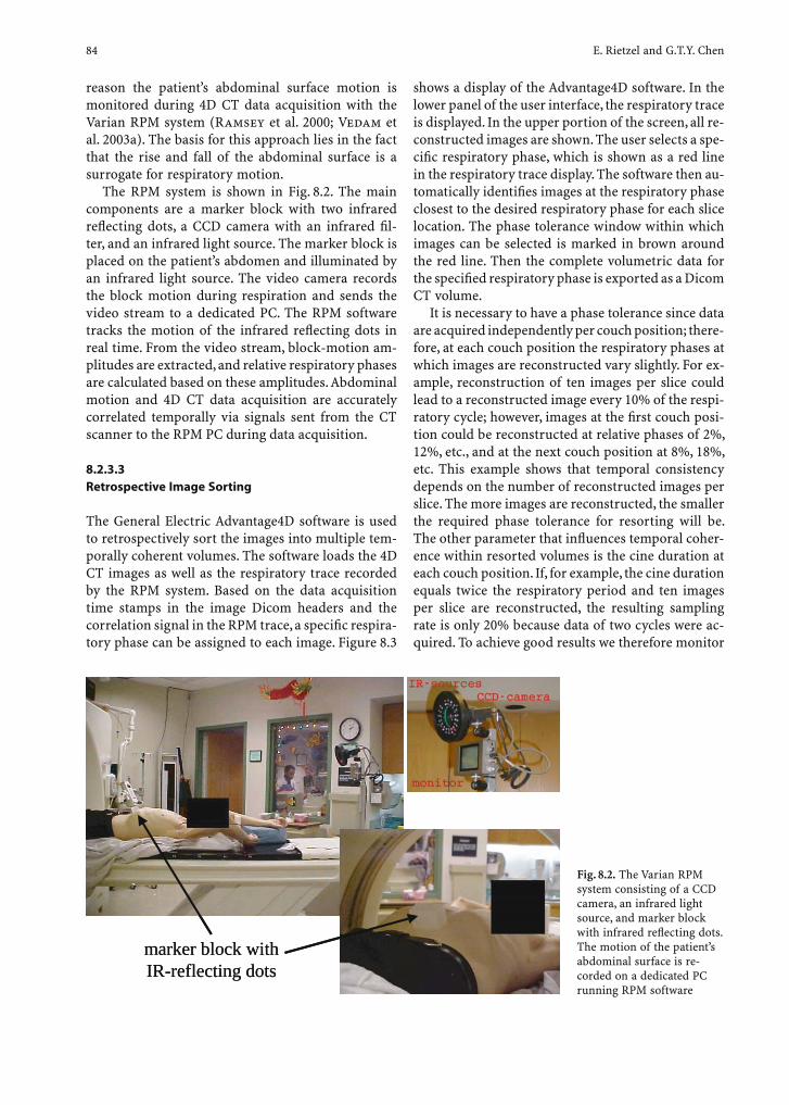
84 E. Rietzel and G.T.Y. Chen

reason the patient’s abdominal surface motion is monitored during 4D CT data acquisition with the Varian RPM system (Ramsey et al. 2000; Vedam et al. 2003a). The basis for this approach lies in the fact that the rise and fall of the abdominal surface is a surrogate for respiratory motion.

The RPM system is shown in Fig. 8.2. The main components are a marker block with two infrared refl ecting dots, a CCD camera with an infrared fi l-ter, and an infrared light source. The marker block is placed on the patient’s abdomen and illuminated by an infrared light source. The video camera records the block motion during respiration and sends the video stream to a dedicated PC. The RPM software tracks the motion of the infrared refl ecting dots in real time. From the video stream, block-motion am-plitudes are extracted, and relative respiratory phases are calculated based on these amplitudes. Abdominal motion and 4D CT data acquisition are accurately correlated temporally via signals sent from the CT scanner to the RPM PC during data acquisition.

8.2.3.3 Retrospective Image Sorting

The General Electric Advantage4D software is used to retrospectively sort the images into multiple tem-porally coherent volumes. The software loads the 4D CT images as well as the respiratory trace recorded by the RPM system. Based on the data acquisition time stamps in the image Dicom headers and the correlation signal in the RPM trace, a specifi c respira-tory phase can be assigned to each image. Figure 8.3

shows a display of the Advantage4D software. In the lower panel of the user interface, the respiratory trace is displayed. In the upper portion of the screen, all re-constructed images are shown. The user selects a spe-cifi c respiratory phase, which is shown as a red line in the respiratory trace display. The software then au-tomatically identifi es images at the respiratory phase closest to the desired respiratory phase for each slice location. The phase tolerance window within which images can be selected is marked in brown around the red line. Then the complete volumetric data for the specifi ed respiratory phase is exported as a Dicom CT volume.

It is necessary to have a phase tolerance since data are acquired independently per couch position; there-fore, at each couch position the respiratory phases at which images are reconstructed vary slightly. For ex-ample, reconstruction of ten images per slice could lead to a reconstructed image every 10% of the respi-ratory cycle; however, images at the fi rst couch posi-tion could be reconstructed at relative phases of 2%, 12%, etc., and at the next couch position at 8%, 18%, etc. This example shows that temporal consistency depends on the number of reconstructed images per slice. The more images are reconstructed, the smaller the required phase tolerance for resorting will be. The other parameter that infl uences temporal coher-ence within resorted volumes is the cine duration at each couch position. If, for example, the cine duration equals twice the respiratory period and ten images per slice are reconstructed, the resulting sampling rate is only 20% because data of two cycles were ac-quired. To achieve good results we therefore monitor

Fig. 8.2. The Varian RPM system consisting of a CCD camera, an infrared light source, and marker block with infrared refl ecting dots. The motion of the patient’s abdominal surface is re-corded on a dedicated PC running RPM software

marker block with IR-reflecting dotsmarker block with IR-reflecting dots

4D Imaging and Treatment Planning 85

the patient’s respiratory cycle for several minutes be-fore 4D CT data acquisition starts.

During the 4D CT retrospective sorting process, data acquired at different respiratory cycles are assem-bled into one volume, since one respiratory cycle per couch position is required. Figure 8.4 shows respira-tory traces of different patients. The upper row shows the complete respiratory trace during a 4D CT data ac-quisition, end inhalation at the top, and end exhalation at the bottom. Note the rapidly changing variations at peak inhalation from breath to breath and the slow drifting baseline at peak exhalation. Currently it is not clear how well an external motion surrogate, such as the marker block, represents internal anatomic mo-tion. Abdominal motion is measured at one point only so differences between chest and abdominal breathing

cannot be easily detected. Using relative respiratory phases for data re-sorting allows assembling full vol-umes for different phases. Using the respiratory am-plitudes instead would result in many volumes with missing slices. On the other hand, it could very well be that respiratory phases represent internal motion better than amplitudes observed at a single point only. This is an area of current active research.

The mid and lower graphs in Fig. 8.4 show enlarged regions of the respiratory trace for two other patients. Whereas the patient in the middle breathed with a re-producible wave form, the patient in the lower graph held his/her breath several times during data acqui-sition. The resulting re-sorted volumes therefore showed poor temporal coherence. The CT images from these examples are presented in Fig. 8.8.

Fig. 8.3. General Electric Advantage4D software for retrospective sorting of 4D CT data into temporally coherent volumes. The main panel shows all images reconstructed. The ones selected for the current respiratory phase are marked with a light blue square. The lower panel shows the patient’s respiratory trace during 4D CT data acquisition. The currently selected respiratory phase is indicated by a red line. Phase tolerances required for re-sorting a complete volume are shown as a brown band. Different respiratory phases can be selected in the control panel on the left

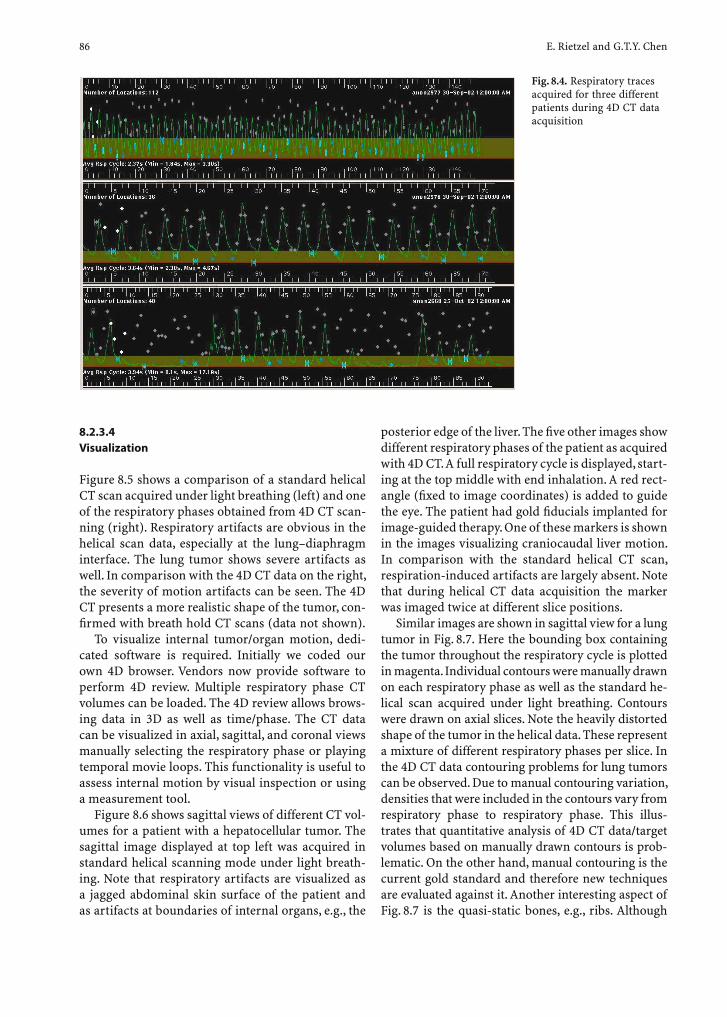
86 E. Rietzel and G.T.Y. Chen

8.2.3.4 Visualization

Figure 8.5 shows a comparison of a standard helical CT scan acquired under light breathing (left) and one of the respiratory phases obtained from 4D CT scan-ning (right). Respiratory artifacts are obvious in the helical scan data, especially at the lung–diaphragm interface. The lung tumor shows severe artifacts as well. In comparison with the 4D CT data on the right, the severity of motion artifacts can be seen. The 4D CT presents a more realistic shape of the tumor, con-fi rmed with breath hold CT scans (data not shown).

To visualize internal tumor/organ motion, dedi-cated software is required. Initially we coded our own 4D browser. Vendors now provide software to perform 4D review. Multiple respiratory phase CT volumes can be loaded. The 4D review allows brows-ing data in 3D as well as time/phase. The CT data can be visualized in axial, sagittal, and coronal views manually selecting the respiratory phase or playing temporal movie loops. This functionality is useful to assess internal motion by visual inspection or using a measurement tool.

Figure 8.6 shows sagittal views of different CT vol-umes for a patient with a hepatocellular tumor. The sagittal image displayed at top left was acquired in standard helical scanning mode under light breath-ing. Note that respiratory artifacts are visualized as a jagged abdominal skin surface of the patient and as artifacts at boundaries of internal organs, e.g., the

posterior edge of the liver. The fi ve other images show different respiratory phases of the patient as acquired with 4D CT. A full respiratory cycle is displayed, start-ing at the top middle with end inhalation. A red rect-angle (fi xed to image coordinates) is added to guide the eye. The patient had gold fi ducials implanted for image-guided therapy. One of these markers is shown in the images visualizing craniocaudal liver motion. In comparison with the standard helical CT scan, respiration-induced artifacts are largely absent. Note that during helical CT data acquisition the marker was imaged twice at different slice positions.

Similar images are shown in sagittal view for a lung tumor in Fig. 8.7. Here the bounding box containing the tumor throughout the respiratory cycle is plotted in magenta. Individual contours were manually drawn on each respiratory phase as well as the standard he-lical scan acquired under light breathing. Contours were drawn on axial slices. Note the heavily distorted shape of the tumor in the helical data. These represent a mixture of different respiratory phases per slice. In the 4D CT data contouring problems for lung tumors can be observed. Due to manual contouring variation, densities that were included in the contours vary from respiratory phase to respiratory phase. This illus-trates that quantitative analysis of 4D CT data/target volumes based on manually drawn contours is prob-lematic. On the other hand, manual contouring is the current gold standard and therefore new techniques are evaluated against it. Another interesting aspect of Fig. 8.7 is the quasi-static bones, e.g., ribs. Although

Fig. 8.4. Respiratory traces acquired for three different patients during 4D CT data acquisition

4D Imaging and Treatment Planning 87

Fig. 8.5. Standard helical CT scan acquired under light breathing (left) in comparison with one respiratory phase of a 4D CT scan (right). For the 4D CT scan, scan length was reduced. Typical motion artifacts seen in the standard helical scan are absent in the 4D CT volume

Fig. 8.6. Standard helical CT scan acquired under light breathing (top left) as well as fi ve respiratory phases obtained from 4D CT scanning. The 4D CT phases are displayed for a full respiratory cycle. The patient had radio-opaque markers implanted in the liver for image guidance. A box was plotted to visualize respiratory motion. Note that the displayed marker is imaged in two adjacent slices in the helical scan

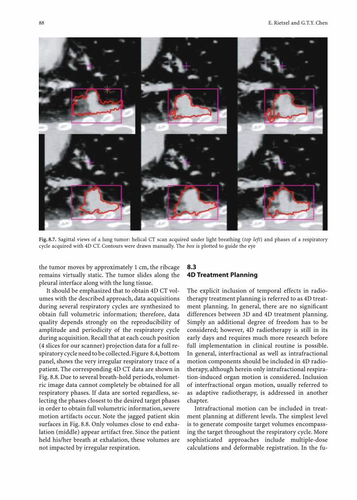
88 E. Rietzel and G.T.Y. Chen

the tumor moves by approximately 1 cm, the ribcage remains virtually static. The tumor slides along the pleural interface along with the lung tissue.

It should be emphasized that to obtain 4D CT vol-umes with the described approach, data acquisitions during several respiratory cycles are synthesized to obtain full volumetric information; therefore, data quality depends strongly on the reproducibility of amplitude and periodicity of the respiratory cycle during acquisition. Recall that at each couch position (4 slices for our scanner) projection data for a full re-spiratory cycle need to be collected. Figure 8.4, bottom panel, shows the very irregular respiratory trace of a patient. The corresponding 4D CT data are shown in Fig. 8.8. Due to several breath-hold periods, volumet-ric image data cannot completely be obtained for all respiratory phases. If data are sorted regardless, se-lecting the phases closest to the desired target phases in order to obtain full volumetric information, severe motion artifacts occur. Note the jagged patient skin surfaces in Fig. 8.8. Only volumes close to end exha-lation (middle) appear artifact free. Since the patient held his/her breath at exhalation, these volumes are not impacted by irregular respiration.

8.3 4D Treatment Planning

The explicit inclusion of temporal effects in radio-therapy treatment planning is referred to as 4D treat-ment planning. In general, there are no signifi cant differences between 3D and 4D treatment planning. Simply an additional degree of freedom has to be considered; however, 4D radiotherapy is still in its early days and requires much more research before full implementation in clinical routine is possible. In general, interfractional as well as intrafractional motion components should be included in 4D radio-therapy, although herein only intrafractional respira-tion-induced organ motion is considered. Inclusion of interfractional organ motion, usually referred to as adaptive radiotherapy, is addressed in another chapter.

Intrafractional motion can be included in treat-ment planning at different levels. The simplest level is to generate composite target volumes encompass-ing the target throughout the respiratory cycle. More sophisticated approaches include multiple-dose calculations and deformable registration. In the fu-

Fig. 8.7. Sagittal views of a lung tumor: helical CT scan acquired under light breathing (top left) and phases of a respiratory cycle acquired with 4D CT. Contours were drawn manually. The box is plotted to guide the eye

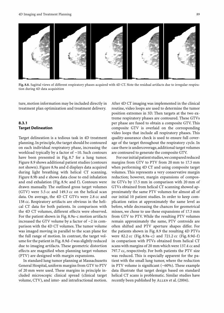
4D Imaging and Treatment Planning 89

ture, motion information may be included directly in treatment plan optimization and treatment delivery.

8.3.1 Target Delineation

Target delineation is a tedious task in 4D treatment planning. In principle, the target should be contoured on each individual respiratory phase, increasing the workload typically by a factor of ~10. Such contours have been presented in Fig. 8.7 for a lung tumor. Figure 8.9 shows additional patient studies (contours not shown). Figure 8.9a and d displays data acquired during light breathing with helical CT scanning. Figure 8.9b and e shows data close to end inhalation and end exhalation (Fig. 8.9c and f). Contours were drawn manually. The outlined gross target volumes (GTV) were 5.5 cc and 149.3 cc on the helical scan data. On average, the 4D CT GTVs were 2.8 cc and 158 cc. Respiratory artifacts are obvious in the heli-cal CT data for both patients. In comparison with the 4D CT volumes, different effects were observed. For the patient shown in Fig. 8.9a–c motion artifacts increased the GTV volume by a factor of ~2 in com-parison with the 4D CT volumes. The tumor volume was imaged moving in parallel to the scan plane for the full range of motion. In contrast, the target vol-ume for the patient in Fig. 8.9d–f was slightly reduced due to imaging artifacts. These geometric distortion effects are magnifi ed when planning target volumes (PTV) are designed with margin expansions.

In standard lung tumor planning at Massachusetts General Hospital, uniform margins from GTV to PTV of 20 mm were used. These margins in principle in-cluded microscopic clinical spread (clinical target volume, CTV), and inter- and intrafractional motion.

After 4D CT imaging was implemented in the clinical routine, video loops are used to determine the tumor position extremes in 3D. Then targets at the two ex-treme respiratory phases are contoured. These GTVs per phase are fused to obtain a composite GTV. This composite GTV is overlaid on the corresponding video loops that include all respiratory phases. This quality-assurance check is used to ensure full cover-age of the target throughout the respiratory cycle. In case there is undercoverage, additional target volumes are contoured to generate the composite GTV.

For our initial patient studies, we compared reduced margins from GTV to PTV from 20 mm to 17.5 mm when performing 4D CT and using composite target volumes. This represents a very conservative margin reduction; however, margin expansions of compos-ite GTVs by 17.5 mm in comparison with 20 mm of GTVs obtained from helical CT scanning showed ap-proximately the same PTV volumes for almost all of our initial 10 patient studies. In order to keep com-plication ratios at approximately the same level as before, while decreasing the chances for geometrical misses, we chose to use these expansions of 17.5 mm from GTV to PTV. While the resulting PTV volumes remain approximately the same, PTV centroids are often shifted and PTV aperture shapes differ. For the patients shown in Fig. 8.9 the resulting 4D PTVs were 82.2 cc (Fig. 8.9a–c) and 721.2 cc (Fig. 8.9d–f) in comparison with PTVs obtained from helical CT scans with margins of 20 mm which were 137.4 cc and 797.7 cc, respectively. For both patients the PTV size was reduced. This is especially apparent for the pa-tient with the small lung tumor, where the reduction in PTV volume is signifi cant (~60%). These example data illustrate that target design based on standard helical CT scans is problematic. Similar studies have recently been published by Allen et al. (2004).

Fig. 8.8. Sagittal views of different respiratory phases acquired with 4D CT. Note the residual artifacts due to irregular respira-tion during 4D data acquisition

90 E. Rietzel and G.T.Y. Chen

8.3.2 Fast Segmentation of Lung Tumors

Manual contouring of several respiratory phases for research is feasible. In clinical routine, however, other segmentation techniques need to be developed. One possibility was described above, that is contouring se-lected extreme phases and fusing two targets. For lung tumors, the large density difference between tumor and surrounding lung can be exploited to propose an effi cient segmentation approach to multiple CT data sets from 4D CT data. The calculation of a maximum intensity volume (MIV) as shown in Fig. 8.10 can be used for contouring a composite target volume on one CT data set. A maximum intensity volume is calculated based on all respiratory phases available. For each individual voxel throughout the time vary-ing image volume, the maximum voxel density at each point from all respiratory phase volumes is de-termined. This procedure identifi es all high-density voxels in the resulting volume and therefore shows the full extent of the tumor throughout the respira-tory cycle. Figure 8.10, left, shows an axial slice of a maximum intensity volume. Figure 8.10, right, shows the corresponding end-inhalation and end-exhala-tion respiratory states of the 4D CT volumes color coded. The tumor at inspiration is shown in green, at expiration in red. Wherever densities match the overlay image appears in yellow. The example shows the potential of MIVs, and the lung tumor, includ-ing respiratory motion, can be manually contoured

with a single contour rather than ten (one for each phase); however, to date, the MIV concept has not been fully tested. Currently it should only be used for initial contouring in combination with validation as overlay on respiratory phase videos. When a tumor is adjacent to other high-density objects, such as the mediastinum, MIV-based contouring of the compos-ite GTV might be inappropriate, since portions of the moving mediastinum can occlude the tumor in some respiratory phases.

8.3.3 Digitally Reconstructed Fluoroscopy

Traditionally organ/tumor motion is often assessed by fl uoroscopy on the conventional simulator. For many soft tissue tumors, direct visualization of tu-mors is not possible with projection radiography/fl uoroscopy. In such cases, motion of surrounding organs or implanted fi ducial markers can be used as surrogates for tumor motion (Balter et al. 2001). Utilizing 4D CT, marker motion can directly be re-lated to tumor motion in 3D. It is possible to estimate lung tumor motion in some cases with fl uoroscopy; however, the precise extent and shape of the lung tumor often cannot be visualized.

Calculation of digitally reconstructed radiographs (DRR) at each respiratory phase based on 4D CT vol-umes can help in determining the exact position or extent of the tumor in 2D projections. Figure 8.11

Fig. 8.9. Sagittal (a–c) and coronal (d–f) views of two lung tumor patients. a, d Standard helical CT scans acquired under light breath-ing. b, e End inspiration. c, f End expiration of 4D CT data

ba c

ed f

4D Imaging and Treatment Planning 91

shows three respiratory phases of a lung cancer pa-tient. The upper row displays coronal views through the center of the GTV, the lower row shows images of the corresponding DRRs. Without 4D CT data, the DRRs are diffi cult to interpret and the tumor position and extent are ambiguous. With additional informa-tion from the 4D data, displayed side by side, tumor outlines are more easily detectable. Furthermore, it is useful to project GTV contours delineated at each respiratory phase on the corresponding DRRs to even better describe the tumor position in the DRRs.

An animation of several DRRs can be considered digitally reconstructed fl uoroscopy (DRF). The DRF is useful for beam gating or tracking based on fl uo-roscopic data acquired directly during treatment de-livery. The fl uoroscopy stream can then directly be compared with the DRF that corresponds to respira-tory states of the patient known from 4D CT. Another possibility to use DRFs is in validating breathing models of an individual patient. Rather than acquir-ing multiple 4D CTs, several respiratory cycles could be recorded with fl uoroscopy and compared with the

Fig. 8.10. Maximum in-tensity volume (MIV) of a lung tumor (left) and cor-responding end-inhalation (green) and end-expiration (red) breath-hold CT scans as color overlay (right)

INSP - EXPINSP - EXPMIVMIV

Fig. 8.11. Coronal views of 4D CT data for three respiratory phases of a lung tumor patient (top) and corresponding digitally reconstructed fl uoroscopy images (bottom)

92 E. Rietzel and G.T.Y. Chen

DRF. With recently available treatment technology, specifi cally on-board imaging on linear accelerators, this may even be performed on a daily basis prior to treatment delivery.

8.3.4 Dose Calculations

4D CT data provide the ability to study the impact of respiratory motion on dose distributions. We have implemented 4D dose calculations in our commer-cial treatment planning system FOCUS (CMS). Since current treatment planning systems do not offer 4D dose calculations, the multiple dose calculations are set up in the underlying Unix fi le system using a set of shell scripts and C-code. Based on a specifi c set of treatment plan parameters (e.g., beam angles, weights, MUs per fi eld, etc.), dose calculations can be performed at each respiratory phase.

The current implementation is on a research basis only. A treatment plan is optimized for one CT vol-ume state. Then this treatment plan is copied to the study sets of all respiratory phases. We have imple-mented multiple dose calculations for 3D conformal radiotherapy, IMRT, and proton therapy. For proton therapy the dose calculations can be submitted to a

Linux cluster in order to perform all dose calcula-tions in parallel. For photons the individual dose cal-culations are initiated through the standard graphi-cal user interface of the treatment planning system. For IMRT, interplay effects between organ motion and dynamic beam delivery have not yet been imple-mented. The current implementation for 4D IMRT dose calculations is equivalent to IMRT as delivered through a compensator. Interplay effects cannot yet be implemented easily since precise temporal model-ing of organ motion and MLC motion during irradia-tion are required.

Figure 8.12 shows coronal views at different re-spiratory phases of a 4D dose distribution. A treat-ment plan was optimized based on a standard heli-cal CT scan for 3D conformal radiotherapy (data not shown). Then dose distributions were re-calculated for several respiratory phases obtained from 4D CT. Parameters of the treatment plan were not altered.

Changes in anatomy, especially the lung tumor po-sition, as well as slight distortions of the displayed isodose lines, are visible; however, the shape of the isodose lines and their relative position to patient anatomy remain nearly identical, predominantly in medium and low-dose regions. Typically, changes in dose deposition are overestimated when examining isodose lines. Even small variations in dose deposi-

Fig. 8.12. Dose distributions calculated for 4D CT volumes of a full respira-tory cycle. The treatment plan was optimized for a volume of a standard helical CT scan. Parameters were cop-ied to other respiratory phases for dose calculations

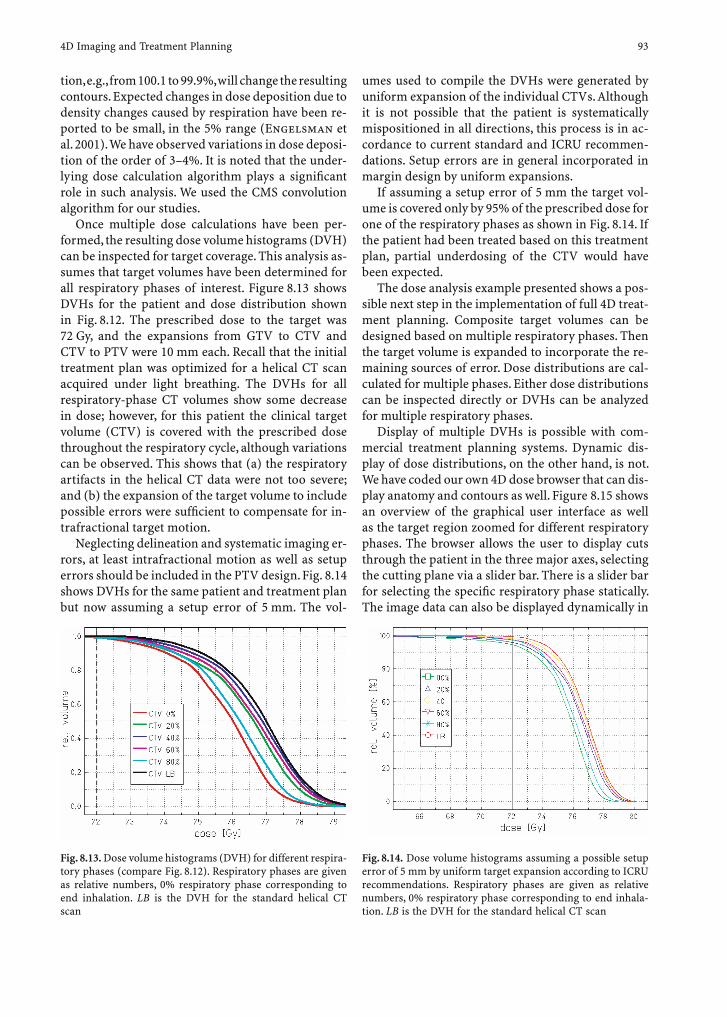
4D Imaging and Treatment Planning 93

tion, e.g., from 100.1 to 99.9%, will change the resulting contours. Expected changes in dose deposition due to density changes caused by respiration have been re-ported to be small, in the 5% range (Engelsman et al. 2001). We have observed variations in dose deposi-tion of the order of 3–4%. It is noted that the under-lying dose calculation algorithm plays a signifi cant role in such analysis. We used the CMS convolution algorithm for our studies.

Once multiple dose calculations have been per-formed, the resulting dose volume histograms (DVH) can be inspected for target coverage. This analysis as-sumes that target volumes have been determined for all respiratory phases of interest. Figure 8.13 shows DVHs for the patient and dose distribution shown in Fig. 8.12. The prescribed dose to the target was 72 Gy, and the expansions from GTV to CTV and CTV to PTV were 10 mm each. Recall that the initial treatment plan was optimized for a helical CT scan acquired under light breathing. The DVHs for all respiratory-phase CT volumes show some decrease in dose; however, for this patient the clinical target volume (CTV) is covered with the prescribed dose throughout the respiratory cycle, although variations can be observed. This shows that (a) the respiratory artifacts in the helical CT data were not too severe; and (b) the expansion of the target volume to include possible errors were suffi cient to compensate for in-trafractional target motion.

Neglecting delineation and systematic imaging er-rors, at least intrafractional motion as well as setup errors should be included in the PTV design. Fig. 8.14 shows DVHs for the same patient and treatment plan but now assuming a setup error of 5 mm. The vol-

umes used to compile the DVHs were generated by uniform expansion of the individual CTVs. Although it is not possible that the patient is systematically mispositioned in all directions, this process is in ac-cordance to current standard and ICRU recommen-dations. Setup errors are in general incorporated in margin design by uniform expansions.

If assuming a setup error of 5 mm the target vol-ume is covered only by 95% of the prescribed dose for one of the respiratory phases as shown in Fig. 8.14. If the patient had been treated based on this treatment plan, partial underdosing of the CTV would have been expected.

The dose analysis example presented shows a pos-sible next step in the implementation of full 4D treat-ment planning. Composite target volumes can be designed based on multiple respiratory phases. Then the target volume is expanded to incorporate the re-maining sources of error. Dose distributions are cal-culated for multiple phases. Either dose distributions can be inspected directly or DVHs can be analyzed for multiple respiratory phases.

Display of multiple DVHs is possible with com-mercial treatment planning systems. Dynamic dis-play of dose distributions, on the other hand, is not. We have coded our own 4D dose browser that can dis-play anatomy and contours as well. Figure 8.15 shows an overview of the graphical user interface as well as the target region zoomed for different respiratory phases. The browser allows the user to display cuts through the patient in the three major axes, selecting the cutting plane via a slider bar. There is a slider bar for selecting the specifi c respiratory phase statically. The image data can also be displayed dynamically in

Fig. 8.13. Dose volume histograms (DVH) for different respira-tory phases (compare Fig. 8.12). Respiratory phases are given as relative numbers, 0% respiratory phase corresponding to end inhalation. LB is the DVH for the standard helical CT scan

Fig. 8.14. Dose volume histograms assuming a possible setup error of 5 mm by uniform target expansion according to ICRU recommendations. Respiratory phases are given as relative numbers, 0% respiratory phase corresponding to end inhala-tion. LB is the DVH for the standard helical CT scan

94 E. Rietzel and G.T.Y. Chen

a video loop. Dose distributions are overlaid in color-wash mode. The browser is useful for fast inspection of 4D dose distributions.

8.3.5 Non-Rigid Registration

To add dose distributions of different respiratory cy-cles non-rigid registration is needed. Each individual anatomical voxel position must be tracked through-out the respiratory cycle in order to accurately assess deposited dose. The tracking of voxel positions can be accomplished by registration of CT volumes which includes the modeling of local deformations.

Non-rigid registrations of liver have recently been reported in the literature by Brock et al. (2003) using thin-plate splines. We have chosen to use the freeware tool vtkCISG developed at King’s College in London (Hartkens et al. 2002). The toolkit registers organ volumes at different (respiratory/deformed) states to each other. Full affi ne transformations including translations, rotations, scaling, and shearing as well as local deformations are supported. Local deforma-tions are modeled with B-splines (Rueckert et al. 1999). A control point grid is superimposed to the pa-tient anatomy. Each of the knots of the grid is moved during registration. The underlying anatomy follows the motion of the translated knots. Registration in general is an optimization problem. The parameter to be optimized is the similarity between the two vol-

umes to be registered. Within the optimization loop the control points are translated and the resulting deformations to the anatomy are calculated. Then the similarity between the target volume and the de-formed volume is computed. A variety of similarity measures is offered in vtkCISG. We have chosen to use sum of squared differences (SSD) as similarity measure for most registrations. To obtain the simi-larity between two volumes voxels at corresponding positions are subtracted. Then the sum over all differ-ences squared is used to assess overall similarity.

Figure 8.16 shows the results obtained for registra-tion of end inhalation to end exhalation for a patient with a hepatocellular tumor. The top row displays the patient anatomy at these respiratory states. To com-pare the CT data visually, color overlays are used. In the bottom row end exhalation is color coded in yellow, end inhalation in blue. Wherever densities between the different respiratory states match the resulting color is on a gray scale. Transformation pa-rameters were optimized for a full-affi ne registration followed by modeling local deformations as described above. The arrows indicate the transformations from end inhalation to end exhalation for different regions of the anatomy.

Figure 8.16 shows the good performance of the registration process; high-density structures are in good agreement. The different lengths and directions of the displacement vectors illustrate that modeling of local deformations is essential to obtain precise registration results.

Fig. 8.15. Four-dimensional browsing software. Displayed are anatomy as well as dose distribution (left). Three different respira-tory phases are shown (right)

4D Imaging and Treatment Planning 95

One important step in obtaining good registra-tion results has not yet been addressed: adequate pre-processing of the data. The internal anatomy of the patient was segmented prior to registration. This is necessary because the ribcage, for example, hardly moves during respiration, whereas the liver right next to it moves signifi cantly. Due to intrinsic smoothness constraints B-splines cannot model such abrupt ana-tomical changes. Independently moving anatomy has to be separated from each other prior to registration; otherwise, different parts compete against each other during registration. This would then lead to insuffi -cient registration results as well as breaking of bones, for example.

8.3.6 Total Dose Distributions in the Presence of Respiratory Motion

Once dose calculations per respiratory phase have been performed and non-rigid registration pa-rameters between different respiratory phases have been optimized, total dose distributions, including

respiratory motion, can be calculated. Dose distribu-tions are deformed according to the parameters ob-tained from non-rigid CT–CT registration to ensure tracking of the dose within each voxel throughout the respiratory cycle. For the patient presented in Fig. 8.15, Fig. 8.17 shows the original dose distribu-tion for end inhalation as well as the dose distribu-tion for end exhalation mapped to end inhalation. In this frame of reference patient anatomy is static, whereas dose distributions move according to the underlying respiratory motion. This is most obvious when comparing the relative position of the CTV (purple) to the isodose lines. In addition, the shape of individual isodose lines changes, most obvious left of the CTV.

After non-rigid transformation to one reference respiratory phase dose distributions can be added on a voxel-by-voxel basis to obtain a total dose distri-bution. Accurate tracking of the dose deposited per individual voxel throughout the respiratory cycle is guaranteed by the transformations. The DVHs for the dose distributions in Fig. 8.17 are plotted in Fig. 8.18 for individual respiratory phases as well as for the to-tal dose distribution including respiratory motion.

Fig. 8.16. Non-rigid registration of internal patient anatomy. Top: end exhalation (left) and end inhalation (right); bottom: color overlays before (left) and after registration (right). Transformations are indicated by red arrows

96 E. Rietzel and G.T.Y. Chen

8.4 Conclusion

The presence of intrafractional target motion is a major challenge in radiotherapy. This chapter has surveyed the technical issues to utilize 4D imaging data in treatment planning of respiration induced organ motion. 4D imaging can be applied to mark-edly reduce the artifacts that can occur in scanning moving objects. The imaging technique used at Massachusetts General Hospital captures anatomy at multiple respiratory states, increasing the image data by a factor of ~10. The benefi t of 4D imaging is

that it provides a more accurate estimate of the true target shape and its trajectory as a function of time. This information can help improve the precision of external beam irradiation.

The initial method we implemented in utilizing 4D CT involved defi ning composite volumes that com-bined target volumes at the extremes of motion ob-served. Our observations from this implementation indicate that 4D target volumes differ from those derived by conventional helical scanning. What can change is that the shapes of volumes of interest and their centroids change, and they are more accurate from 4D CT. Utilization of 4D CT image data in treat-ment planning has also been implemented and pro-vides information on how organ motion can perturb dose distributions. A key technology in the calcu-lation of dose to moving organs is deformable im-age registration. Other technical challenges that are needed include visualization and segmentation tools that are designed to deal with dynamic image data.

There are a number of caveats to be kept in mind when considering dose to moving targets. Our focus has been solely on the effects of respiratory motion. We do not consider cardiac motion, or interfractional motion, due to either setup errors or variations in physiologic state, e.g., stomach-size variations that could infl uence positions of adjacent organs. The data acquired in 4D CT is synthesized from multiple breaths during an acquisition time of a few minutes. Reproducibility of this pattern during each treatment fraction is implicitly assumed when analyzing the re-sulting 4D dose distributions. Possible variations may be monitored by examining the respiratory trace on a daily basis – either the abdominal surface or even

Fig. 8.17. Deformation of a dose distribution according to non-rigid CT–CT registration parameters to a reference respiratory phase. Corresponding transformations are indicated by red arrows (right)

Fig. 8.18. Dose volume histograms for fi ve respiratory phases and the total dose distribution including respiratory motion. Respiratory phases are given as relative numbers, 0% respira-tory phase corresponding to end inhalation

4D Imaging and Treatment Planning 97

better the target volume directly, e.g., using fl uoros-copy.

In the future, techniques to deliver 4D treatment will be explored, developed, and refi ned to take full advantage of the new knowledge provided by 4D CT. Image-guided therapy in the treatment room could well include 4D cone-beam CT, if appropriate. The global view of irradiation of moving targets involves knowledge and control of the entire process from im-aging for planning to daily irradiation. This knowl-edge will lead to methods to mitigate the dose-per-turbing effects of motion, and possibly lead to safe decrease of geometric margins and increased thera-peutic gain.

References

Allen AM, Siracuse KM, Hayman JA et al. (2004) Evaluation of the infl uence of breathing on the movement and modeling of lung tumors. Int J Radiat Oncol Biol Phys 58:1251–1257

Balter JM, Ten Haken RK, Lawrence TS et al. (1996) Uncer-tainties in CT-based radiation therapy planning associ-ated with patient breathing. Int J Radiat Oncol Biol Phys 36:167–174

Balter JM, Lam KL, McGinn CJ et al. (1998) Improvement of CT-based treatment planning model of abdominal targets using static exhale imaging. Int J Radiat Oncol Biol Phys 41:939–943

Balter JM, Dawson LA, Kazanjian S et al. (2001) Determina-tion of ventilatory liver movement via radiographic evalu-ation of diaphragm position. Int J Radiat Oncol Biol Phys 51:267–270

Brock KK, McShan DL, Ten Haken RK et al. (2003) Automated generation of a four-dimensional model of the liver using warping and mutual information. Med Phys 30:1128–1133

Chen GT, Kung JH, Beaudette KP (2004) Artifacts in computed tomography scanning of moving objects. Semin Radiat Oncol 14:19–26

Engelsman M, Damen EM, de Jaeger K et al. (2001) The effect of breathing and set-up errors on the cumulative dose to a lung tumor. Radiother Oncol 60:95–105

Ford EC, Mageras GS, Yorke E et al. (2003) Respiration-corre-lated spiral CT: a method of measuring respiratory-induced anatomic motion for radiation treatment planning. Med Phys 30:88–97

Hartkens T, Rueckert D, Schnabel JA et al. (2002) VTK CISG

Registration Toolkit. An open source software package for affi ne and non-rigid registration of single- and multimodal 3D images. In: Meiler M, Saupe D, Kruggel F, Handels H, Lehmann T (eds) Bildverarbeitung für die Medizin Algo-rithmen - Systeme - Anwendungen. Workshop proceedings, Leipzig March 2002, series: Informatik aktuell. Springer, Berlin Heidelberg New York

ICRU50 (1993) Prescribing, recording and reporting photon beam therapy. ICRU, Bethesda, Maryland

ICRU62 (1999) Prescribing, recording and reporting photon beam therapy (supplement to ICRU Rep 50). ICRU, Bethesda, Maryland

Low DA, Nystrom M, Kalinin E et al. (2003) A method for the reconstruction of four-dimensional synchronized CT scans acquired during free breathing. Med Phys 30:1254–1263

Pan T, Lee TY, Rietzel E et al. (2004) 4D-CT imaging of a volume infl uenced by respiratory motion on multi-slice CT. Med Phys 31:333–340

Ramsey CR, Scaperoth D, Arwood D et al. (2000) Clinical expe-rience with a commercial respiratory gating system. Int J Radiat Oncol Biol Phys 48:164–165

Rietzel E, Chen GTY, Choi NC et al. (2005a) 4D image based treatment planning: target volume segmentation and dose calculations in the presence of respiratory motion. Int J Radiat Oncol Biol Phys 61:1535–1550

Rietzel E, Pan T, Chen GTY (2005b) 4D computed tomog-raphy: image formation and clinical protocol. Med Phys 32:874–889

Ritchie CJ, Hsieh J, Gard MF et al. (1994) Predictive respiratory gating: a new method to reduce motion artifacts on CT scans. Radiology 190:847–852

Ross CS, Hussey DH, Pennington EC et al. (1990) Analysis of movement of intrathoracic neoplasms using ultrafast computerized tomography. Int J Radiat Oncol Biol Phys 18:671–677

Rueckert D, Sonoda LI, Hayes C et al. (1999) Non-rigid regis-tration using free-form deformations: application to breast MR images. IEEE Trans Med Imaging 18:712–721

Shimizu S, Shirato H, Kagei K et al. (2000) Impact of respira-tory movement on the computed tomographic images of small lung tumors in three-dimensional (3D) radiotherapy. Int J Radiat Oncol Biol Phys 46:1127–1133

Vedam SS, Kini VR, Keall PJ et al. (2003a) Quantifying the pre-dictability of diaphragm motion during respiration with a noninvasive external marker. Med Phys 30:505–513

Vedam SS, Keall PJ, Kini VR et al. (2003b) Acquiring a four-dimensional computed tomography data set using an external respiratory signal. Phys Med Biol 48:45–62

Wagman R, Yorke E, Giraud P et al. (2003) Reproducibility of organ position with respiratory gating for liver tumors: use in dose-escalation. Int J Radiat Oncol Biol Phys 55:659–668

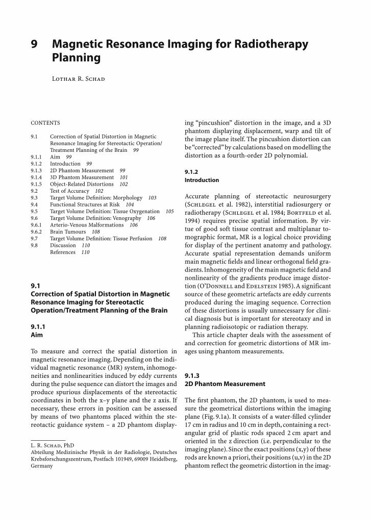
Magnetic Resonance Imaging for Radiotherapy Planning 99

9 Magnetic Resonance Imaging for Radiotherapy Planning

Lothar R. Schad

L. R. Schad, PhDAbteilung Medizinische Physik in der Radiologie, Deutsches Krebsforschungszentrum, Postfach 101949, 69009 Heidelberg, Germany

9.1 Correction of Spatial Distortion in Magnetic Resonance Imaging for Stereotactic Operation/Treatment Planning of the Brain

9.1.1 Aim

To measure and correct the spatial distortion in magnetic resonance imaging. Depending on the indi-vidual magnetic resonance (MR) system, inhomoge-neities and nonlinearities induced by eddy currents during the pulse sequence can distort the images and produce spurious displacements of the stereotactic coordinates in both the x–y plane and the z axis. If necessary, these errors in position can be assessed by means of two phantoms placed within the ste-reotactic guidance system – a 2D phantom display-

ing “pincushion” distortion in the image, and a 3D phantom displaying displacement, warp and tilt of the image plane itself. The pincushion distortion can be “corrected” by calculations based on modelling the distortion as a fourth-order 2D polynomial.

9.1.2 Introduction

Accurate planning of stereotactic neurosurgery (Schlegel et al. 1982), interstitial radiosurgery or radiotherapy (Schlegel et al. 1984; Bortfeld et al. 1994) requires precise spatial information. By vir-tue of good soft tissue contrast and multiplanar to-mographic format, MR is a logical choice providing for display of the pertinent anatomy and pathology. Accurate spatial representation demands uniform main magnetic fi elds and linear orthogonal fi eld gra-dients. Inhomogeneity of the main magnetic fi eld and nonlinearity of the gradients produce image distor-tion (O’Donnell and Edelstein 1985). A significant source of these geometric artefacts are eddy currents produced during the imaging sequence. Correction of these distortions is usually unnecessary for clini-cal diagnosis but is important for stereotaxy and in planning radioisotopic or radiation therapy.

This article chapter deals with the assessment of and correction for geometric distortions of MR im-ages using phantom measurements.

9.1.3 2D Phantom Measurement

The fi rst phantom, the 2D phantom, is used to mea-sure the geometrical distortions within the imaging plane (Fig. 9.1a). It consists of a water-fi lled cylinder 17 cm in radius and 10 cm in depth, containing a rect-angular grid of plastic rods spaced 2 cm apart and oriented in the z direction (i.e. perpendicular to the imaging plane). Since the exact positions (x,y) of these rods are known a priori, their positions (u,v) in the 2D phantom refl ect the geometric distortion in the imag-

CONTENTS

9.1 Correction of Spatial Distortion in Magnetic Resonance Imaging for Stereotactic Operation/ Treatment Planning of the Brain 999.1.1 Aim 999.1.2 Introduction 999.1.3 2D Phantom Measurement 999.1.4 3D Phantom Measurement 1019.1.5 Object-Related Distortions 1029.2 Test of Accuracy 1029.3 Target Volume Defi nition: Morphology 1039.4 Functional Structures at Risk 1049.5 Target Volume Defi nition: Tissue Oxygenation 1059.6 Target Volume Defi nition: Venography 1069.6.1 Arterio-Venous Malformations 1069.6.2 Brain Tumours 1089.7 Target Volume Defi nition: Tissue Perfusion 1089.8 Discussion 110 References 110

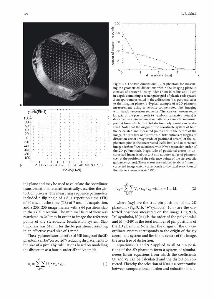
100 L. R. Schad

ing plane and may be used to calculate the coordinate transformation that mathematically describes the dis-tortion process. The measuring sequence parameters included a fl ip angle of 15∞, a repetition time (TR) of 40 ms, an echo time (TE) of 7 ms, one acquisition, and a 256¥256 image matrix with a 64 partition slab in the axial direction. The minimal fi eld of view was restricted to 260 mm in order to image the reference points of the stereotactic localization system. Slab thickness was 64 mm for the 64 partitions, resulting in an effective voxel size of 1 mm3.

The x–y plane distortion of axial MR images of the 2D phantom can be “corrected” (reducing displacements to the size of a pixel) by calculations based on modelling the distortion as a fourth-order 2D polynomial:

N

uk = Â Â Uij . xki . ykj, (1) i,j=0

N

vk = Â Â Vij . xki . ykj with k = 1 ... M, (2) i,j=0

where (x,y) are the true pin positions of the 2D phantom (Fig. 9.1b, “+”symbols); (u,v) are the dis-torted positions measured on the image (Fig. 9.1b, “x” symbols), N (=4) is the order of the polynomial, and M (=249) is the total number of pin positions of the 2D phantom. Note that the origin of the u,v co-ordinate system corresponds to the origin of the x,y coordinate system and lies in the centre of the image, the area free of distortion.

Equations 9.1 and 9.2 applied to all M pin posi-tions of the 2D phantom form a system of simulta-neous linear equations from which the coeffi cients Uij and Vij can be calculated and the distortion cor-rected. Thereby, the selection of N=4 is a compromise between computational burden and reduction in dis-

Fig. 9.1. a The two-dimensional (2D) phantom for measur-ing the geometrical distortions within the imaging plane. It consists of a water-fi lled cylinder 17 cm in radius and 10 cm in depth, containing a rectangular grid of plastic rods spaced 2 cm apart and oriented in the z direction (i.e., perpendicular to the imaging plane). b Typical example of a 2D phantom measurement using a velocity-compensated fast imaging with steady precession sequence. The a priori known regu-lar grid of the plastic rods (+ symbols: calculated points) is deformed to a pincushion-like pattern (x symbols: measured points) from which the 2D-distortion polynomial can be de-rived. Note that the origin of the coordinate system of both the calculated and measured points lies in the centre of the image, the area free of distortion. c Distributions of lengths of distortion vector (magnitude of positional errors) of the 2D phantom pins in the uncorrected (solid line) and in corrected image (broken line) calculated with N=4 (expansion order of the 2D polynomial). Magnitude of positional errors in un-corrected image is about 2–3 mm at outer range of phantom (i.e., at the position of the reference points of the stereotactic guidance system). These errors are reduced to about 1 mm in corrected image which corresponds to the pixel resolution of the image. (From Schad 1995)

a

c

b

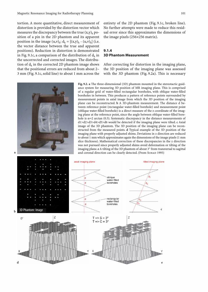
Magnetic Resonance Imaging for Radiotherapy Planning 101

tortion. A more quantitative, direct measurement of distortion is provided by the distortion vector which measures the discrepancy between the true (x,y)k po-sition of a pin in the 2D phantom and its apparent position in the image (u,v)k: dk = |(x,y)k - (u,v)k| (i.e. the vector distance between the true and apparent positions). Reduction in distortion is demonstrated in Fig. 9.1c, a comparison of the distribution of dk in the uncorrected and corrected images. The distribu-tion of dk in the corrected 2D phantom image shows that the positional errors are reduced from about 2–3 mm (Fig. 9.1c, solid line) to about 1 mm across the

entirety of the 2D phantom (Fig. 9.1c, broken line). No further attempts were made to reduce this resid-ual error since this approximates the dimensions of the image pixels (256¥256 matrix).

9.1.4 3D Phantom Measurement

After correcting for distortion in the imaging plane, the 3D position of the imaging plane was assessed with the 3D phantom (Fig. 9.2a). This is necessary

Fig. 9.2. a The three-dimensional (3D) phantom mounted in the stereotactic guid-ance system for measuring 3D position of MR imaging plane. This is comprised of a regular grid of water-fi lled rectangular boreholes, with oblique water-fi lled boreholes in between. This produces a pattern of reference points surrounded by measurement points in axial image from which the 3D position of the imaging plane can be reconstructed. b A 3D-phantom measurement. The distance d be-tween reference point (rectangular water-fi lled borehole) and measurement point (oblique water-fi lled borehole) is a direct measure of the z coordinate of the imag-ing plane at the reference point, since the angle between oblique water-fi lled bore-hole is a=2 arctan (0.5). Systematic discrepancy in the distance measurements of d1>d2>d3>d4>d5>d6 would be detected if the imaging plane were tilted. c Axial image of the 3D phantom. The 3D position of the imaging plane can be recon-structed from the measured points. d Typical example of the 3D position of the imaging plane with properly adjusted shims. Deviations in z direction are reduced to about 1 mm which approximates again the dimensions of the image pixels (1 mm slice thickness). Mathematical correction of these discrepancies in the z direction was not pursued since properly adjusted shims avoid deformation or tilting of the imaging plane. e A tilting of the 3D phantom of about 3∞ from transversal to sagittal and coronal direction can be clearly detected. (From Schad 1995)

3D Phantom: Imageb

a

c

ed

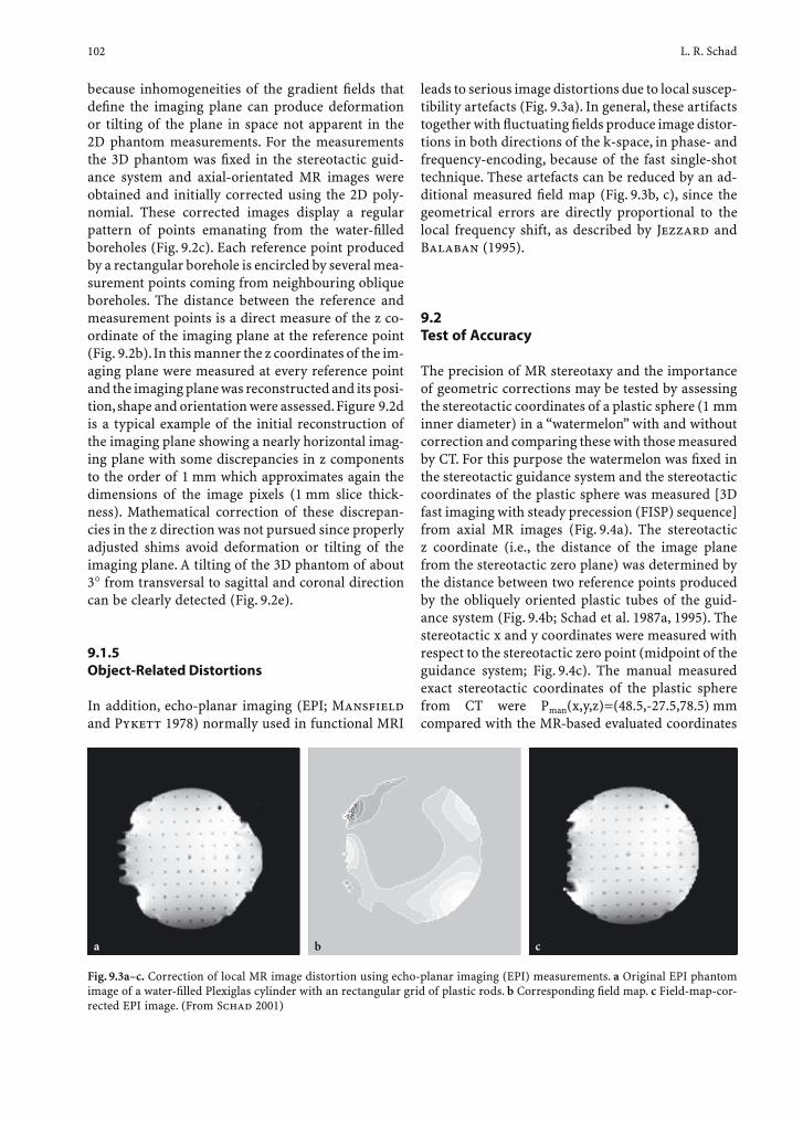
102 L. R. Schad

because inhomogeneities of the gradient fi elds that defi ne the imaging plane can produce deformation or tilting of the plane in space not apparent in the 2D phantom measurements. For the measurements the 3D phantom was fi xed in the stereotactic guid-ance system and axial-orientated MR images were obtained and initially corrected using the 2D poly-nomial. These corrected images display a regular pattern of points emanating from the water-fi lled boreholes (Fig. 9.2c). Each reference point produced by a rectangular borehole is encircled by several mea-surement points coming from neighbouring oblique boreholes. The distance between the reference and measurement points is a direct measure of the z co-ordinate of the imaging plane at the reference point (Fig. 9.2b). In this manner the z coordinates of the im-aging plane were measured at every reference point and the imaging plane was reconstructed and its posi-tion, shape and orientation were assessed. Figure 9.2d is a typical example of the initial reconstruction of the imaging plane showing a nearly horizontal imag-ing plane with some discrepancies in z components to the order of 1 mm which approximates again the dimensions of the image pixels (1 mm slice thick-ness). Mathematical correction of these discrepan-cies in the z direction was not pursued since properly adjusted shims avoid deformation or tilting of the imaging plane. A tilting of the 3D phantom of about 3∞ from transversal to sagittal and coronal direction can be clearly detected (Fig. 9.2e).

9.1.5 Object-Related Distortions

In addition, echo-planar imaging (EPI; Mansfi eld and Pykett 1978) normally used in functional MRI

leads to serious image distortions due to local suscep-tibility artefacts (Fig. 9.3a). In general, these artifacts together with fl uctuating fi elds produce image distor-tions in both directions of the k-space, in phase- and frequency-encoding, because of the fast single-shot technique. These artefacts can be reduced by an ad-ditional measured fi eld map (Fig. 9.3b, c), since the geometrical errors are directly proportional to the local frequency shift, as described by Jezzard and Balaban (1995).

9.2 Test of Accuracy

The precision of MR stereotaxy and the importance of geometric corrections may be tested by assessing the stereotactic coordinates of a plastic sphere (1 mm inner diameter) in a “watermelon” with and without correction and comparing these with those measured by CT. For this purpose the watermelon was fi xed in the stereotactic guidance system and the stereotactic coordinates of the plastic sphere was measured [3D fast imaging with steady precession (FISP) sequence] from axial MR images (Fig. 9.4a). The stereotactic z coordinate (i.e., the distance of the image plane from the stereotactic zero plane) was determined by the distance between two reference points produced by the obliquely oriented plastic tubes of the guid-ance system (Fig. 9.4b; Schad et al. 1987a, 1995). The stereotactic x and y coordinates were measured with respect to the stereotactic zero point (midpoint of the guidance system; Fig. 9.4c). The manual measured exact stereotactic coordinates of the plastic sphere from CT were Pman(x,y,z)=(48.5,-27.5,78.5) mm compared with the MR-based evaluated coordinates

Fig. 9.3a–c. Correction of local MR image distortion using echo-planar imaging (EPI) measurements. a Original EPI phantom image of a water-fi lled Plexiglas cylinder with an rectangular grid of plastic rods. b Corresponding fi eld map. c Field-map-cor-rected EPI image. (From Schad 2001)

ba c

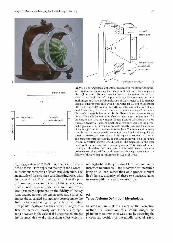
Magnetic Resonance Imaging for Radiotherapy Planning 103

not negligible at the position of the reference points, increases nonlinearly – the z component measured lying on an “arc” rather than on a proper “straight line”; hence, disparity of these two measurements increases with increasing z coordinate.

9.3 Target Volume Defi nition: Morphology

In addition, an anatomic check of the correction method (i.e. correction of anatomic images via phantom measurements) was done by assessing the stereotactic position of the middle cerebral artery

Fig. 9.4. a The “watermelon phantom” mounted in the stereotactic guid-ance system for measuring the precision of MR stereotaxy. A plastic phere (1 mm inner diameter) was implanted in the watermelon and the stereotactic coordinates of the plastic sphere were evaluated in trans-axial images at CT and MR. b Evaluation of the stereotactic z-coordinate. Plexiglas squares embedded with a steel wires for CT or b plastic tubes fi lled with Gd-DTPA solution for MR are attached to the stereotactic head frame and give reference points in transaxial images. The z coor-dinate of an image is determined by the distance between two reference points. The angle between the reference tubes is =2 arctan (0.5). The crossing point of two tubes lies in the zero plane of the stereotactic head frame. c A transaxial image shows the tube reference points of the stereo-tactic guidance system. The z coordinate directly measures the distance of the image from the stereotactic zero-plane. The stereotactic x and y coordinates are measured with respect to the midpoint of the guidance system (=stereotactic zero point). A discrepancy between uncorrected and corrected images of about 2 m appeared mainly in the z coordinate without correction of geometric distortion. The magnitude of the error in z coordinate increases with increasing z-value. This is related in part to the pincushion-like distortion pattern of the axial images, since z co-ordinates are calculated from and therefore ultimately dependent on the fi delity of the x,y components. (From Schad et al. 1987a)

ba

c

Pima(x,y,z)=(47.6,-27.7,78.0) mm, whereas discrepan-cies of about 2 mm appeared mainly in the z coordi-nate without correction of geometric distortion. The magnitude of the error in z coordinate increases with the z coordinate. This is related in part to the pin-cushion-like distortion pattern of the axial images, since z coordinates are calculated from and there-fore ultimately dependent on the fi delity of the x,y components. In both the uncorrected and corrected images the calculated z component correspond to the distance between the x,y components of two refer-ence points. Ideally, and in the corrected images, this distance increases linearly with the true z compo-nent; however, in the case of the uncorrected images the distance, due to the pincushion effect which is

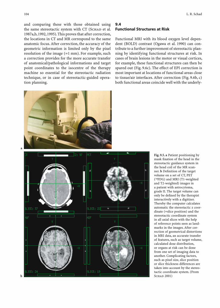
104 L. R. Schad

and comparing these with those obtained using the same stereotactic system with CT (Schad et al. 1987a,b, 1992, 1995). This proves that after correction, the locations in CT and MR correspond to the same anatomic focus. After correction, the accuracy of the geometric information is limited only by the pixel resolution of the image (=1 mm). For example, such a correction provides for the more accurate transfer of anatomical/pathological informations and target point coordinates to the isocentre of the therapy machine so essential for the stereotactic radiation technique, or in case of stereotactic-guided opera-tion planning.

9.4 Functional Structures at Risk

Functional MRI with its blood oxygen level depen-dent (BOLD) contrast (Ogawa et al. 1990) can con-tribute to a further improvement of stereotactic plan-ning by identifying functional structures at risk. In cases of brain lesions in the motor or visual cortices, for example, these functional structures can then be spared out (Fig. 9.6c). The effect of EPI correction is most important at locations of functional areas close to tissue/air interfaces. After correction (Fig. 9.6b, c) both functional areas coincide well with the underly-

Fig. 9.5. a Patient positioning by mask fi xation of the head in the stereotactic guidance system in the head coil of the MR scan-ner. b Defi nition of the target volume on a set of CT, PET (18FDG) and MRI (T1-weighted and T2-weighted) images in a patient with astrocytoma, grade II. The target volume can only be defi ned by the therapist interactively with a digitizer. Thereby the computer calculates automatic the stereotactic z coor-dinate (=slice position) and the stereotactic coordinate system in all axial slices with the help of reference points seen as land-marks in the images. After cor-rection of geometrical distortions in MRI data, an accurate transfer of features, such as target volume, calculated dose distribution, or organs at risk can be done from one set of imaging data to another. Complicating factors, such as pixel size, slice position or slice thickness differences are taken into account by the stereo-tactic coordinate system. (From Schad 2001)b

a

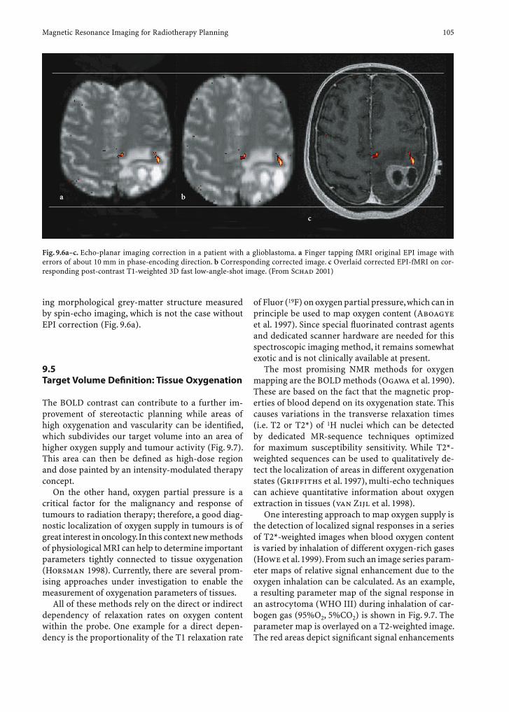
Magnetic Resonance Imaging for Radiotherapy Planning 105

ing morphological grey-matter structure measured by spin-echo imaging, which is not the case without EPI correction (Fig. 9.6a).

9.5 Target Volume Defi nition: Tissue Oxygenation

The BOLD contrast can contribute to a further im-provement of stereotactic planning while areas of high oxygenation and vascularity can be identifi ed, which subdivides our target volume into an area of higher oxygen supply and tumour activity (Fig. 9.7). This area can then be defi ned as high-dose region and dose painted by an intensity-modulated therapy concept.

On the other hand, oxygen partial pressure is a critical factor for the malignancy and response of tumours to radiation therapy; therefore, a good diag-nostic localization of oxygen supply in tumours is of great interest in oncology. In this context new methods of physiological MRI can help to determine important parameters tightly connected to tissue oxygenation (Horsman 1998). Currently, there are several prom-ising approaches under investigation to enable the measurement of oxygenation parameters of tissues.

All of these methods rely on the direct or indirect dependency of relaxation rates on oxygen content within the probe. One example for a direct depen-dency is the proportionality of the T1 relaxation rate

of Fluor (19F) on oxygen partial pressure, which can in principle be used to map oxygen content (Aboagye et al. 1997). Since special fl uorinated contrast agents and dedicated scanner hardware are needed for this spectroscopic imaging method, it remains somewhat exotic and is not clinically available at present.

The most promising NMR methods for oxygen mapping are the BOLD methods (Ogawa et al. 1990). These are based on the fact that the magnetic prop-erties of blood depend on its oxygenation state. This causes variations in the transverse relaxation times (i.e. T2 or T2*) of 1H nuclei which can be detected by dedicated MR-sequence techniques optimized for maximum susceptibility sensitivity. While T2*-weighted sequences can be used to qualitatively de-tect the localization of areas in different oxygenation states (Griffi ths et al. 1997), multi-echo techniques can achieve quantitative information about oxygen extraction in tissues (van Zijl et al. 1998).

One interesting approach to map oxygen supply is the detection of localized signal responses in a series of T2*-weighted images when blood oxygen content is varied by inhalation of different oxygen-rich gases (Howe et al. 1999). From such an image series param-eter maps of relative signal enhancement due to the oxygen inhalation can be calculated. As an example, a resulting parameter map of the signal response in an astrocytoma (WHO III) during inhalation of car-bogen gas (95%O2, 5%CO2) is shown in Fig. 9.7. The parameter map is overlayed on a T2-weighted image. The red areas depict signifi cant signal enhancements

Fig. 9.6a–c. Echo-planar imaging correction in a patient with a glioblastoma. a Finger tapping fMRI original EPI image with errors of about 10 mm in phase-encoding direction. b Corresponding corrected image. c Overlaid corrected EPI-fMRI on cor-responding post-contrast T1-weighted 3D fast low-angle-shot image. (From Schad 2001)

ba

c

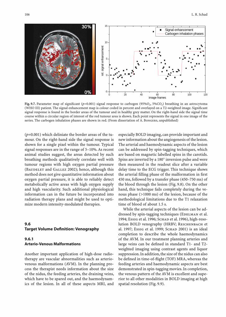
106 L. R. Schad

(p=0.001) which deliniate the border areas of the tu-mour. On the right-hand side the signal response is shown for a single pixel within the tumour. Typical signal responses are in the range of 5–10%. As recent animal studies suggest, the areas detected by such breathing methods qualitatively correlate well with tumour regions with high oxygen partial pressure (Baudelet and Gallez 2002); hence, although this method does not give quantitative information about oxygen partial pressure, it is able to reliably detect metabolically active areas with high oxygen supply and high vascularity. Such additional physiological information can in the future be incorporated into radiation therapy plans and might be used to opti-mize modern intensity-modulated therapies.

9.6 Target Volume Defi nition: Venography

9.6.1 Arterio-Venous Malformations

Another important application of high-dose radio-therapy are vascular abnormalities such as arterio-venous malformations (AVM). In the planning pro-cess the therapist needs information about the size of the nidus, the feeding arteries, the draining veins, which have to be spared out, and the haemodynam-ics of the lesion. In all of these aspects MRI, and

especially BOLD imaging, can provide important and new information about the angiogenesis of the lesion. The arterial and haemodynamic aspects of the lesion can be addressed by spin-tagging techniques, which are based on magnetic labelled spins in the carotids. Spins are inverted by a 180∞ inversion pulse and were then measured in the readout slice after a variable delay time to the ECG trigger. This technique shows the arterial fi lling phase of the malformation in fi rst 450 ms, followed by a transfer phase (450–750 ms) of the blood through the lesion (Fig. 9.8). On the other hand, this technique fails completely during the ve-nous phase (>1000 ms) of the lesion, because of the methodological limitations due to the T1 relaxation time of blood of about 1.5 s.

While the arterial aspects of the lesion can be ad-dressed by spin-tagging techniques (Edelman et al. 1994; Essig et al. 1996; Schad et al. 1996), high-reso-lution BOLD venography (HRBV; Reichenbach et al. 1997; Essig et al. 1999; Schad 2001) is an ideal completion to describe the whole haemodynamics of the AVM. In our treatment planning arteries and large veins can be defi ned in standard T1- and T2-weighted imaging using contrast agents and liquor suppression. In addition, the size of the nidus can also be defi ned in time-of-fl ight (TOF) MRA, whereas the feeding arteries and haemodynamic aspects are best demonstrated in spin-tagging movies. In completion, the venous pattern of the AVM is excellent and supe-rior to all other modalities in BOLD imaging at high spatial resolution (Fig. 9.9).

0 20 40 60 80 100 120-5

0

5

10

15 Signal enhancement Carbogen inhalation phases

rel.

signa

l enh

ance

men

timage frames

Fig. 9.7. Parameter map of signifi cant (p=0.001) signal response to carbogen (95%O2, 5%CO2) breathing in an astrocytoma (WHO III) patient. The signal enhancement map is colour coded in percent and overlayed on a T2-weighted image. Signifi cant signal response is found in the border areas of the tumour and in healthy grey matter. On the right-hand side the signal time course within a circular region of interest of the red tumour area is shown. Each point represents the signal in one image of the series. The carbogen inhalation phases are shown in red. (From dissertation of A. Bongers, unpublished)

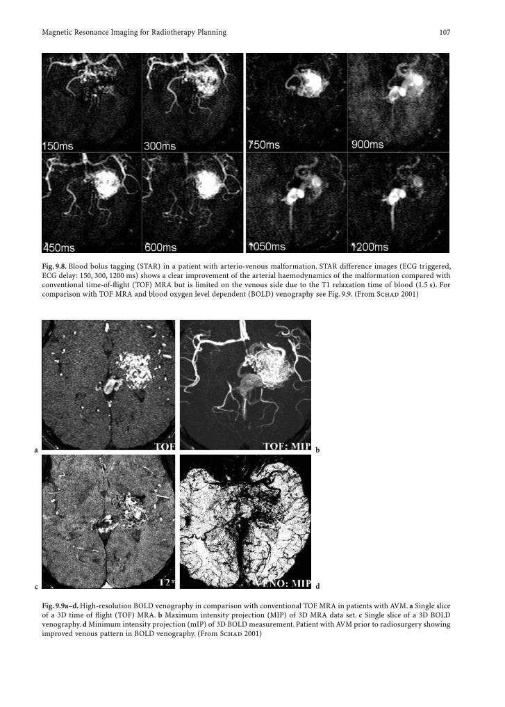
Magnetic Resonance Imaging for Radiotherapy Planning 107

Fig. 9.8. Blood bolus tagging (STAR) in a patient with arterio-venous malformation. STAR difference images (ECG triggered, ECG delay: 150, 300, 1200 ms) shows a clear improvement of the arterial haemodynamics of the malformation compared with conventional time-of-fl ight (TOF) MRA but is limited on the venous side due to the T1 relaxation time of blood (1.5 s). For comparison with TOF MRA and blood oxygen level dependent (BOLD) venography see Fig. 9.9. (From Schad 2001)

Fig. 9.9a–d. High-resolution BOLD venography in comparison with conventional TOF MRA in patients with AVM. a Single slice of a 3D time of fl ight (TOF) MRA. b Maximum intensity projection (MIP) of 3D MRA data set. c Single slice of a 3D BOLD venography. d Minimum intensity projection (mIP) of 3D BOLD measurement. Patient with AVM prior to radiosurgery showing improved venous pattern in BOLD venography. (From Schad 2001)

c

ba

d

108 L. R. Schad

Problems appear in patients with AVMs close to tissue/air interfaces. In this case, the malformation cannot be delineated clearly on MR venography and the size of the lesion is underestimated due to suscep-tibility artefacts caused by the presence of adjacent bony structures. Another severe problem appears in patients after subacute bleeding. Thereby contrast-enhanced subtraction and TOF MRA are able to de-pict residual pathological vessels. The MR venogra-phy showed a large area of signal loss due to signal dephasing caused by haemosiderin. The size and shape of the AVM and the origin of the pathological vessels were diffi cult to assess.

9.6.2 Brain Tumours

In cases of patients with brain tumours, MR venog-raphy shows a complex and variable venous pattern.

In case of patients with glioblastoma conventional spin-echo imaging shows a typical pattern of contrast enhancement on T1-weighted imaging, surrounded by a large oedema seen on T2-weighted images. On MR venography a large area of signal loss is present in the necrotic part of the tumour with a different pattern of small veins in the part of the contrast enhancement of the lesion (Fig. 9.10).

9.7 Target Volume Defi nition: Tissue Perfusion

Perfusion measurements using MRI (e.g. contrast-enhanced T1-weighted MRI, arterial spin labelling) are the methods of choice for detection and de-lineation of cerebral metastases during diagnostic work-up and treatment planning, allowing for accu-rate defi nition of the treatment target volume. After

Fig. 9.10a–d. High-resolution BOLD venography (d) in comparison with conventional T1-weighted (a, b) and T2-weighted (c) imaging in patients with brain tumours. Patient with glioblastoma shows an area of signal loss in BOLD venography in the ne-crotic part (d) surrounded by a complex venous pattern in the contrast enhancing part of the tumour (b). (From Schad 2005)

ba

c d

Magnetic Resonance Imaging for Radiotherapy Planning 109

therapy, MRI is used for monitoring the response to treatment and for evaluating radiation-induced side effects. Ideally, MRI would be able to distin-guish between local tumour recurrence, tumour necrosis, and radiation-related defi ciencies of the blood–brain barrier and would be able to predict treatment outcome early. Pulsed arterial spin-label-ling techniques (Detre et al. 1992) have the ability to measure perfusion in an image slice of interest without additional application of contrast agent. Intrinsic water molecules in arterial blood are used as a freely diffusible contrast agent carrying the la-belled magnetization fl ow.

Arterial spin labeling (ASL) techniques, such as fl ow-sensitive alternating inversion recovery (FAIR; Kim 1995), provide a tool to assess relative perfusion (Fig. 9.11). These techniques acquire inversion recov-ery images with a nonselective inversion pulse which fl ips the magnetization of water in arterial blood. The

image is acquired after the infl ow time TI to allow the labelled blood to reach the image slice. To eliminate static tissue signal, these images are subtracted from inversion recovery images with a slice-selective inver-sion pulse placed over readout slice and acquired after the infl ow time TI. The difference image in Fig. 9.11 containing the signal of arterial blood delivered to the image voxel within the infl ow time TI is propor-tional to relative perfusion. Using arterial spin label-ling techniques, absolute perfusion can be assessed using sophisticated MRI sequences (e.g. Q2TIPS, ITS-FAIR) in combination with a general kinetic model (Buxton et al. 1998; Luh et al. 1999) based on a one-compartment model. A clinical example of a patient with glioblastoma is shown in Fig. 9.12. Perfusion-weighted imaging using the Q2TIPS method shows a clear correlation to contrast-enhanced post-Gd-DTPA T1-weighted imaging in areas of high tumour vascularity (Weber et al. 2004).

Fig. 9.11. Principle of fl ow-sensitive alternating inversion recovery arterial spin-labeling technique: inversion slab (red), im-age slice (green). The difference between global and selective inversion results in a perfusion-weighted image. (Courtesy of A. Kroll)

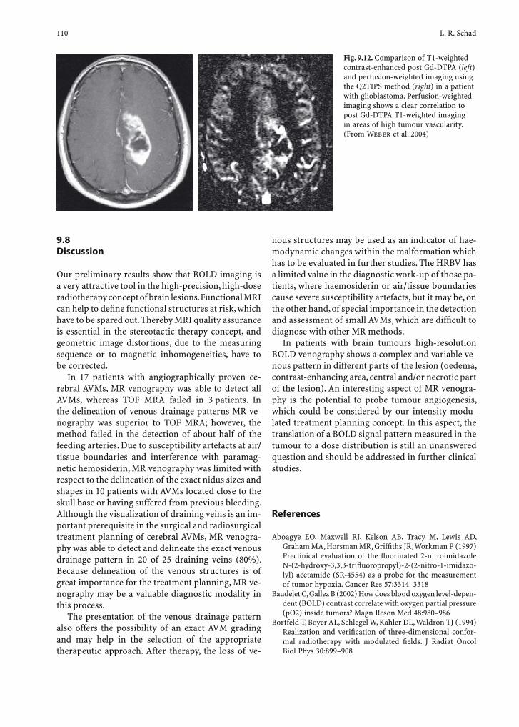
110 L. R. Schad

9.8 Discussion

Our preliminary results show that BOLD imaging is a very attractive tool in the high-precision, high-dose radiotherapy concept of brain lesions. Functional MRI can help to defi ne functional structures at risk, which have to be spared out. Thereby MRI quality assurance is essential in the stereotactic therapy concept, and geometric image distortions, due to the measuring sequence or to magnetic inhomogeneities, have to be corrected.

In 17 patients with angiographically proven ce-rebral AVMs, MR venography was able to detect all AVMs, whereas TOF MRA failed in 3 patients. In the delineation of venous drainage patterns MR ve-nography was superior to TOF MRA; however, the method failed in the detection of about half of the feeding arteries. Due to susceptibility artefacts at air/tissue boundaries and interference with paramag-netic hemosiderin, MR venography was limited with respect to the delineation of the exact nidus sizes and shapes in 10 patients with AVMs located close to the skull base or having suffered from previous bleeding. Although the visualization of draining veins is an im-portant prerequisite in the surgical and radiosurgical treatment planning of cerebral AVMs, MR venogra-phy was able to detect and delineate the exact venous drainage pattern in 20 of 25 draining veins (80%). Because delineation of the venous structures is of great importance for the treatment planning, MR ve-nography may be a valuable diagnostic modality in this process.

The presentation of the venous drainage pattern also offers the possibility of an exact AVM grading and may help in the selection of the appropriate therapeutic approach. After therapy, the loss of ve-

nous structures may be used as an indicator of hae-modynamic changes within the malformation which has to be evaluated in further studies. The HRBV has a limited value in the diagnostic work-up of those pa-tients, where haemosiderin or air/tissue boundaries cause severe susceptibility artefacts, but it may be, on the other hand, of special importance in the detection and assessment of small AVMs, which are diffi cult to diagnose with other MR methods.

In patients with brain tumours high-resolution BOLD venography shows a complex and variable ve-nous pattern in different parts of the lesion (oedema, contrast-enhancing area, central and/or necrotic part of the lesion). An interesting aspect of MR venogra-phy is the potential to probe tumour angiogenesis, which could be considered by our intensity-modu-lated treatment planning concept. In this aspect, the translation of a BOLD signal pattern measured in the tumour to a dose distribution is still an unanswered question and should be addressed in further clinical studies.

References

Aboagye EO, Maxwell RJ, Kelson AB, Tracy M, Lewis AD, Graham MA, Horsman MR, Griffi ths JR, Workman P (1997) Preclinical evaluation of the fl uorinated 2-nitroimidazole N-(2-hy droxy-3,3,3-trifl uoropropyl)-2-(2-nitro-1-imidazo-lyl) acetamide (SR-4554) as a probe for the measurement of tumor hypoxia. Cancer Res 57:3314–3318

Baudelet C, Gallez B (2002) How does blood oxygen level-depen-dent (BOLD) contrast correlate with oxygen partial pressure (pO2) inside tumors? Magn Reson Med 48:980–986

Bortfeld T, Boyer AL, Schlegel W, Kahler DL, Waldron TJ (1994) Realization and verifi cation of three-dimensional confor-mal radiotherapy with modulated fi elds. J Radiat Oncol Biol Phys 30:899–908

Fig. 9.12. Comparison of T1-weighted contrast-enhanced post Gd-DTPA (left) and perfusion-weighted imaging using the Q2TIPS method (right) in a patient with glioblastoma. Perfusion-weighted imaging shows a clear correlation to post Gd-DTPA T1-weighted imaging in areas of high tumour vascularity. (From Weber et al. 2004)

Magnetic Resonance Imaging for Radiotherapy Planning 111

Buxton RB, Frank LR, Wong EC, Siewert B, Warach S, Edel-man RR (1998) A general kinetic model for quantitative perfusion imaging with arterial spin labeling. Magn Res Med 40:383–396

Detre JA, Leigh JS, Williams DS, Koretsky AP (1992) Perfusion imaging. Magn Reson Med 23:37–45

Edelman RR, Siewert B, Adamis M, Gaa J, Laub G, Wielopolski P (1994) Signal targeting with alternating radiofrequency (STAR) sequences: application to MR angiography. Magn Reson Med 31:233–238

Essig M, Engenhart R, Knopp MV, Bock M, Scharf J, Debus J, Wenz F, Hawighorst H, Schad LR, van Kaick G (1996) Cerebral arteriovenous malformations: improved nidus demarcation by means of dynamic tagging MR-angiogra-phy. Magn Reson Imaging 14:227–233

Essig M, Reichenbach JR, Schad LR, Schoenberg SO, Debus J, Kaiser WA (1999) High-resolution MR venography of cerebral arteriovenous malformations. Magn Reson Imag-ing 17:1417–1425

Griffi ths JR, Taylor NJ, Howe FA, Saunders MI, Robinson SP, Hoskin PJ, Powell ME, Thoumine M, Caine LA, Baddeley H (1997) The response of human tumors to carbogen breath-ing, monitored by gradient-recalled echo magnetic reso-nance imaging. Int J Radiat Oncol Biol Phys 39:697–701

Horsman MR (1998) Measurement of tumor oxygenation. Int J Radiat Oncol Biol Phys 42:701–704

Howe FA, Robinson SP, Rodrigues LM, Griffi ths JR (1999) Flow and oxygenation dependent (FLOOD) contrast MR imag-ing to monitor the response of rat tumors to carbogen breathing. Magn Reson Imaging 17:1307–1318

Jezzard P, Balaban RS (1995) Correction of geometric distor-tion in echo planar imaging from B0 fi eld variations. Magn Reson Med 34:65–73

Kim S-G (1995) Quantifi cation of relative cerebral blood fl ow change by fl ow-sensitive alternating inversion recov-ery (FAIR) technique: application to functional mapping. Magn Reson Med 34:293–301

Luh WM, Wong EC, Bandettini PA, Hyde JS (1999) QUIPSS II with thin-slice TI1 periodic saturation: a method for improving accuracy of quantitative perfusion imaging using pulsed arterial spin labeling. Magn Reson Med 41:1246–1254

Mansfi eld P, Pykett IL (1978) Biological and medical imaging by NMR. J Magn Reson 29:355–373

O’Donnell M, Edelstein WA (1985) NMR imaging in the pres-ence of magnetic fi eld inhomogeneities and gradient fi eld nonlinearities. Med Phys 12:20–26

Ogawa S, Lee TM, Nayak AS, Glynn P (1990) Oxygenation-sensitive contrast in magnetic resonance image of rodent brain at high magnetic fi elds. Magn Reson Med 14:68–78

Reichenbach JR, Venkatesan R, Schillinger DJ, Kido DK, Haacke EM (1997) Small vessels in the human brain: MR venogra-

phy with deoxyhemoglobin as an intrinsic contrast agent. Radiology 204:272–277

Schad LR (1995) Correction of spatial distortion in magnetic resonance imaging for stereotactic operation/treatment planning in the brain. In: Hartmann GH (ed) Quality assur-ance program on stereotactic radiosurgery. Springer, Berlin Heidelberg New York, pp 80–89

Schad LR (2001) Improved target volume characterization in stereotactic treatment planning of brain lesions by using high-resolution BOLD MR-venography. NMR Biomed 14:478–483

Schad LR, Lott S, Schmitt F, Sturm V, Lorenz WJ (1987a) Cor-rection of spatial distortion in MR imaging: a prerequisite for accurate stereotaxy. J Comput Assist Tomogr 11:499–505

Schad LR, Boesecke R, Schlegel W, Hartmann G, Sturm V, Strauss L, Lorenz WJ (1987b) Three dimensional image correlation of CT, MR, and PET studies in radiotherapy treatment planning of brain tumours. J Comput Assist Tomogr 11:948–954

Schad LR, Ehricke HH, Wowra B, Layer G, Engenhart R, Kauc-zor HU, Zabel HJ, Brix G, Lorenz WJ (1992) Correction of spatial distortion in magnetic resonance angiography for radiosurgical planning of cerebral arteriovenous malfor-mations. Magn Reson Imaging 10:609–621

Schad LR, Bock M, Baudendistel K, Essig M, Debus J, Knopp MV, Engenhart R, Lorenz WJ (1996) Improved target volume defi nition in radiosurgery of arteriovenous mal-formations by stereotactic correlation of MRA, MRI blood bolus tagging, and functional MRI. Eur Radiol 6:38–45

Schlegel W, Scharfenberg H, Doll J, Pastyr O, Sturm V, Netze-band G, Lorenz WJ (1982) CT-images as the basis of opera-tion planning in stereotactical neurosurgery. Proceedings of First International Symposium on Medical Imaging and Image Interpretation. IEEE Computer Society, Silver Spring, pp 172–177

Schlegel W, Scharfenberg H, Doll J, Hartmann G, Sturm V, Lorenz WJ (1984) Three dimensional dose planning using tomographic data. Proc 8th International Conference on the Use of Computers in Radiation Therapy. IEEE Com-puter Society, Silver Spring, pp 191–196

Van Zijl PCM, Eleff SM, Ulatowski JA, Oja JME, Ulug AM, Traystman RJ, Kauppinen RA (1998) Quantitative assess-ment of blood fl ow, blood volume and blood oxygenation effects in functional magnetic resonance imaging. Nature Med 4:159–167

Weber MA, Thilmann C, Lichy MP, Günther M, Delorme S, Zuna I, Bongers A, Schad LR, Debus J, Kauczor HU, Essig M, Schlemmer HP (2004) Assessment of irradiated brain metastases by means of arterial spin-labeling and dynamic susceptibility-weighted contrast-enhanced perfusion MRI: initial results. Invest Radiol 39:277–287

Potential of Magnetic Resonance Spectroscopy for Radiotherapy Planning 113

10 Potential of Magnetic Resonance Spectroscopy for Radiotherapy Planning Andrea Pirzkall

A. Pirzkall, MDAssistant Adjunct Professor, Departments of Radiation Oncology, Radiology and Neurological Surgery, University of California, San Francisco, 505 Parnassus Avenue, L-75, San Francisco, CA 94143, USA

10.1 Introduction

Metabolic imaging has been gaining increased in-terest and popularity among the radiation oncol-ogy community. The ongoing development of such powerful focal treatment delivery techniques such as intensity modulated radiation therapy (IMRT), ra-diosurgery, and HDR brachytherapy has generated renewed interest in dose escalation, altered fraction-ation schemes, and integrated boost techniques as ways to increase radiation effectiveness while re-ducing side effects. These focused radiation therapy (RT) techniques offer great potential in redefi ning the value of RT in certain disease sites, however, they also demand a more precise picture of the tumor, its ex-tent and heterogeneity, in order to direct more or less dose to the appropriate areas while sparing as much normal tissue as possible (disease-targeted RT). This

“dose painting,” a phrase appropriately coined by Clifton Ling, only makes sense if one knows the “lay of the land.” Both CT and MRI have been provid-ing the underlying sketch (black-and-white picture) used for target defi nition and treatment planning for several decades. They describe the anatomic picture of the tumor and surrounding structures well but they fail to provide information (color) about the functional status, the degree of tumor activity and cellular composition, and the presence of infi ltrative disease or distant spread.

Functional or metabolic imaging is beginning to be used to fi ll this gap and provide the needed color. Techniques for acquiring such data include imaging that exploits glucose or amino acids labeled with ra-dioactive isotopes [positron emission tomography (PET), single photon emission computed tomography (SPECT), and magnetic resonance (MR)-based imaging techniques (perfusion- and diffusion-weighted MRI, magnetic resonance spectroscopy imaging (MRSI)].

This chapter examines multi-voxel proton (1H) MRSI, the most advanced of the MR spectroscopy applications. Three-dimensional multivoxel MRSI has improved the discrimination of cancer from sur-rounding healthy tissue and from necrosis by add-ing metabolic data to the morphologic information provided by MRI. Two major disease sites have been studied at University of California, San Francisco (UCSF) with respect to the potential and actual in-corporation of MRS imaging into the treatment plan-ning process for RT and are the subject of this chap-ter: prostate cancer and brain gliomas. Brain gliomas have traditionally proved diffi cult to image using standard means due to their literally “non-visible” infi ltrative behavior and heterogeneous composition. The extent and location of prostate cancer are simi-larly diffi cult to determine without the aid of MRSI because, although MRI has good sensitivity, it has relatively low specifi city. In these two disease sites, the combination of MRI and MRSI provide the struc-tural and metabolic information required to support an improved assessment of aggressiveness, location, extent and spatial distribution.

CONTENTS

10.1 Introduction 11310.2 MR Spectroscopy Imaging 11410.2.1 Background 11410.2.2 MRSI Technique 11410.2.2.1 Brain 11410.2.2.2 Prostate 11510.2.3 Application of MRSI 11510.2.3.1 Brain 11510.2.3.2 Radiosurgery for Recurrent Gliomas 12010.2.3.3 Treatment Protocol for Newly Diagnosed GBM 12110.2.3.4 Assessing Response to RT 12210.2.4 Prostate 12210.3 Current Limitations and Possible Solutions 12710.4 Conclusion 128 References 128

114 A. Pirzkall

10.2 MR Spectroscopy Imaging

10.2.1 Background

Magnetic resonance imaging (MRI) is a noninva-sive imaging technique that makes use of the fact that certain atomic nuclei, such as 1H, 31P, 19F, and 13C, have inherent spin properties that allow them to acquire discrete amounts of energy in the pres-ence of a static magnetic fi eld. The application of electromagnetic fi elds (nonionizing radiofrequency radiation) at right angles to a static magnetic fi eld causes these nuclei to jump to higher energy levels. After removal of the electromagnetic fi elds, the nuclei subsequently drop back to their original spin states by emitting electromagnetic radiation at a rate that can be characterized by their T1 (spin-lattice) and T2 (spin–spin) relaxation times. A receiver coil detects the emitted radiation and records the time domain of the MR signal that, once processed using a fou-rier transform, reveals the spectrum of intensities and frequencies of the nuclei from different chemical species within the excited volume. The location of peaks in the spectrum defi nes the chemicals within the sample. The peak intensity refl ects their concen-tration. Conventional MRI uses the properties of the protons from water to obtain information about their spatial distribution in different tissues. Specialized radiofrequency pulses and magnetic fi eld gradients are used to label the water signal as a function of space and, after appropriate post-processing, provide an anatomic image of the changes in proton density and relaxation properties.

The MR spectroscopic data is typically acquired by suppressing the large signal from water and allowing the properties of other compounds to be recorded and analyzed. Water suppressed 1H spectroscopy techniques are commercially available for obtaining spectra from selected regions within the brain and prostate and can be combined with additional local-ization techniques to produce either a single spec-trum from a region of interest (single-voxel MRS) or a multidimensional array of spectra from the region of interest [3D multivoxel MRS, MRSI, chemical-shift imaging (CSI)]. The peaks in individual spectra re-fl ect the relative concentrations of cellular chemicals within that spatial location. The peak heights and/or areas under the curve relate to the concentration of the respective metabolites. Differences in these concentrations can be used to distinguish “normal/healthy” tissue from neoplastic or necrotic tissue. As

an effi cient method for obtaining arrays of spatially localized spectra at spatial resolutions of 0.2–1 cc, 3D multivoxel MRSI is of greater potential value than single-voxel MRS in target delineation and monitor-ing response to therapy and allows the generation of maps of the spatial distribution of cellular metabo-lites. This is an ideal representation for integrating the information into RT treatment planning.

A signifi cant advantage of 1H-MRSI over other metabolic imaging techniques is that the data can be obtained as part of a conventional MRI and can be directly overlaid upon each other. This enhances the display of metabolic data and allows it to be cor-related with the anatomy as revealed by MRI. This allows areas of anatomic abnormality to be directly correlated with the corresponding area of metabolic abnormality.

10.2.2 MRSI Technique

10.2.2.1 Brain

Details of the MRI and MRSI examinations that were developed at UCSF have been published previously (Nelson 2001; Nelson et al. 2002). Briefly, MR data are acquired on a 1.5-T scanner (General Electric Medical Systems, Milwaukee, Wis.) using a quadrature head coil. The MR images include axial T1-weighted [pre- and post-gadolinium contrast-enhanced 3D spoiled gradient-echo (SPGR), 1.5-mm slice thick-ness] and axial T2-weighted sequences [fl uid-at-tenuated inversion recovery (FLAIR), 3-mm slice thickness]. At the conclusion of the MRI sequences, a 3D multivoxel MRSI sequence with a 1-cc nomi-nal resolution is performed (TR/TE=1000/144 ms; 12¥12¥8 or 16¥8¥8 phase-encoding matrix) apply-ing PRESS (Point REsolved Spatial Selection) vol-ume localization and very selective saturation (VSS) bands for outer-voxel suppression. In order to allow for the acquisition of control spectra, the PRESS-box volume is positioned so as to extend beyond the suspected disease and to include normal brain from the contralateral hemisphere. The PRESS-box also is positioned to avoid areas of subcutaneous lipid and varying magnetic susceptibility that might compro-mise the quality of the spectra. In some cases this means that it is impossible to cover the entire region of suspected disease. All data are aligned to the MR images obtained immediately prior to the MRSI data (usually the post-contrast T1-weighted image).

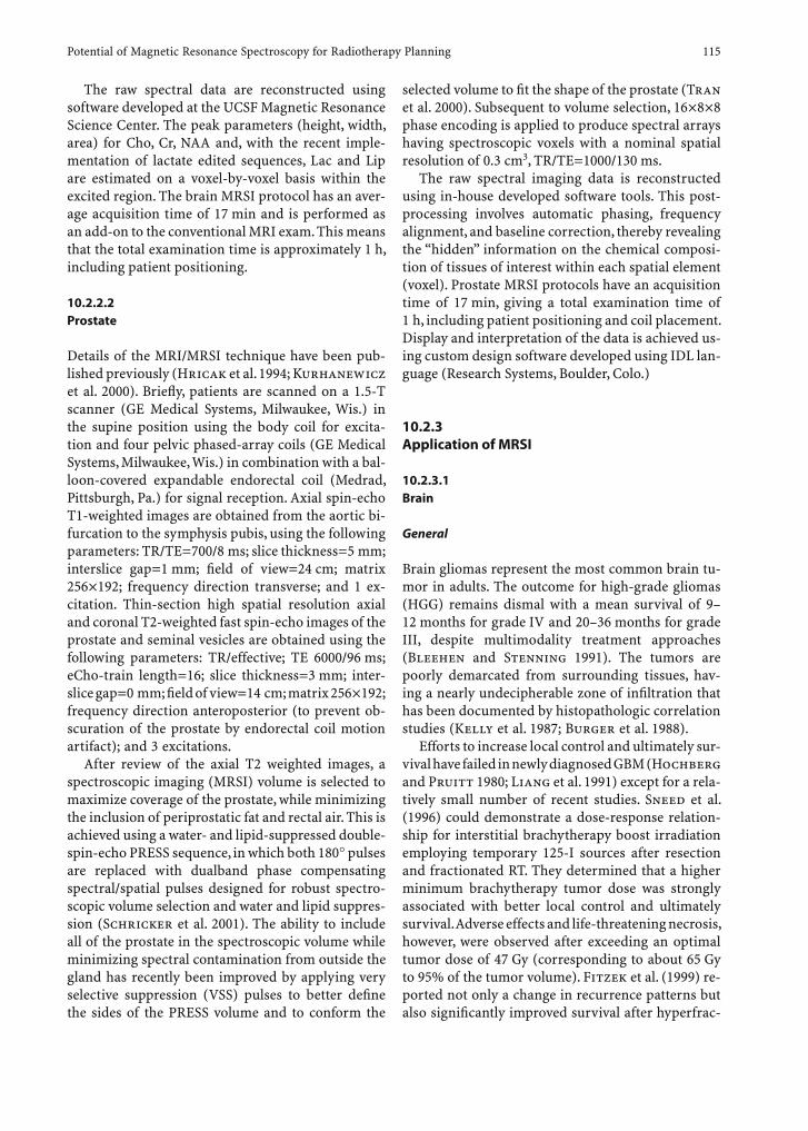
Potential of Magnetic Resonance Spectroscopy for Radiotherapy Planning 115

The raw spectral data are reconstructed using software developed at the UCSF Magnetic Resonance Science Center. The peak parameters (height, width, area) for Cho, Cr, NAA and, with the recent imple-mentation of lactate edited sequences, Lac and Lip are estimated on a voxel-by-voxel basis within the excited region. The brain MRSI protocol has an aver-age acquisition time of 17 min and is performed as an add-on to the conventional MRI exam. This means that the total examination time is approximately 1 h, including patient positioning.

10.2.2.2 Prostate

Details of the MRI/MRSI technique have been pub-lished previously (Hricak et al. 1994; Kurhanewicz et al. 2000). Briefl y, patients are scanned on a 1.5-T scanner (GE Medical Systems, Milwaukee, Wis.) in the supine position using the body coil for excita-tion and four pelvic phased-array coils (GE Medical Systems, Milwaukee, Wis.) in combination with a bal-loon-covered expandable endorectal coil (Medrad, Pittsburgh, Pa.) for signal reception. Axial spin-echo T1-weighted images are obtained from the aortic bi-furcation to the symphysis pubis, using the following parameters: TR/TE=700/8 ms; slice thickness=5 mm; interslice gap=1 mm; fi eld of view=24 cm; matrix 256¥192; frequency direction transverse; and 1 ex-citation. Thin-section high spatial resolution axial and coronal T2-weighted fast spin-echo images of the prostate and seminal vesicles are obtained using the following parameters: TR/effective; TE 6000/96 ms; eCho-train length=16; slice thickness=3 mm; inter-slice gap=0 mm; fi eld of view=14 cm; matrix 256¥192; frequency direction anteroposterior (to prevent ob-scuration of the prostate by endorectal coil motion artifact); and 3 excitations.

After review of the axial T2 weighted images, a spectroscopic imaging (MRSI) volume is selected to maximize coverage of the prostate, while minimizing the inclusion of periprostatic fat and rectal air. This is achieved using a water- and lipid-suppressed double-spin-echo PRESS sequence, in which both 180∞ pulses are replaced with dualband phase compensating spectral/spatial pulses designed for robust spectro-scopic volume selection and water and lipid suppres-sion (Schricker et al. 2001). The ability to include all of the prostate in the spectroscopic volume while minimizing spectral contamination from outside the gland has recently been improved by applying very selective suppression (VSS) pulses to better defi ne the sides of the PRESS volume and to conform the

selected volume to fi t the shape of the prostate (Tran et al. 2000). Subsequent to volume selection, 16¥8¥8 phase encoding is applied to produce spectral arrays having spectroscopic voxels with a nominal spatial resolution of 0.3 cm3, TR/TE=1000/130 ms.

The raw spectral imaging data is reconstructed using in-house developed software tools. This post-processing involves automatic phasing, frequency alignment, and baseline correction, thereby revealing the “hidden” information on the chemical composi-tion of tissues of interest within each spatial element (voxel). Prostate MRSI protocols have an acquisition time of 17 min, giving a total examination time of 1 h, including patient positioning and coil placement. Display and interpretation of the data is achieved us-ing custom design software developed using IDL lan-guage (Research Systems, Boulder, Colo.)

10.2.3 Application of MRSI

10.2.3.1 Brain

General

Brain gliomas represent the most common brain tu-mor in adults. The outcome for high-grade gliomas (HGG) remains dismal with a mean survival of 9–12 months for grade IV and 20–36 months for grade III, despite multimodality treatment approaches (Bleehen and Stenning 1991). The tumors are poorly demarcated from surrounding tissues, hav-ing a nearly undecipherable zone of infi ltration that has been documented by histopathologic correlation studies (Kelly et al. 1987; Burger et al. 1988).

Efforts to increase local control and ultimately sur-vival have failed in newly diagnosed GBM (Hochberg and Pruitt 1980; Liang et al. 1991) except for a rela-tively small number of recent studies. Sneed et al. (1996) could demonstrate a dose-response relation-ship for interstitial brachytherapy boost irradiation employing temporary 125-I sources after resection and fractionated RT. They determined that a higher minimum brachytherapy tumor dose was strongly associated with better local control and ultimately survival. Adverse effects and life-threatening necrosis, however, were observed after exceeding an optimal tumor dose of 47 Gy (corresponding to about 65 Gy to 95% of the tumor volume). Fitzek et al. (1999) re-ported not only a change in recurrence patterns but also signifi cantly improved survival after hyperfrac-

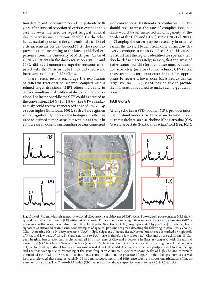
116 A. Pirzkall

tionated mixed photon/proton RT in patients with GBM after surgical resection of various extent. In this case, however, the need for repeat surgical removal due to necrosis was quite considerable. On the other hand, escalating dose in the conventional fashion of 2 Gy increments per day beyond 70 Gy does not im-prove outcome according to the latest published ex-perience from the University of Michigan (Chan et al. 2002). Patients in the dose escalation arms 80 and 90 Gy did not demonstrate superior outcome com-pared with the 70 Gy arm, but they did experience increased incidence of side effects.

These recent results encourage the exploration of different fractionation schemes coupled with a refi ned target defi nition. IMRT offers the ability to deliver simultaneously different doses to different re-gions. For instance, while the CTV could be treated to the conventional 2.0 Gy (or 1.8 Gy), the GTV simulta-neously could receive an increased dose of 2.5–3.0 Gy, or even higher (Pirzkall 2005). Such a dose regimen would signifi cantly increase the biologically effective dose to defi ned tumor areas but would not result in an increase in dose to surrounding organs compared

with conventional 3D stereotactic conformal RT. This should not increase the rate of complications, but there would be an increased inhomogeneity at the border of the GTV and CTV (Thilmann et al. 2001).

Changing the target may be necessary in order to garner the greatest benefi t from differential dose de-livery techniques such as IMRT or RS. In this case, it is critical that the regions identifi ed for special atten-tion be defi ned accurately; namely, that the areas of active tumor (suitable for high dose) must be identi-fi ed separately (as gross tumor volume, GTV) from areas suspicious for tumor extension that are appro-priate to receive a lower dose (classifi ed as clinical target volume, CTV). MRSI may be able to provide the information required to make such target defi ni-tions.

MRSI Analysis

At long echo times (TE=144 ms), MRSI provides infor-mation about tumor activity based on the levels of cel-lular metabolites such as choline (Cho), creatine (Cr), N-acetylaspartate (NAA), and lactate/lipid (Fig. 10.1).

1

23

1

23

1 2

3

1 2

3

1

2 34

1

2 34

55

Fig. 10.1a–d. Patient with left temporo-occipital glioblastoma multiforme (GBM). Axial T1-weighted post-contrast MRI shows typical contrast enhancement (CE) with central necrosis. Three-dimensional magnetic resonance spectroscopy imaging (MRSI) performed within area of excitation [Point REsolved Spatial Selection (PRESS) box, represented by gridlines] reveals metabolic signature of examined brain tissue. Four examples of spectral patterns are given detecting the following metabolites: 1 choline (Cho); 2 creatine (Cr); 3 N-acetylaspartate (NAA); 4 lipid (Lip); and 5 lactate (Lac). Normal brain tissue is marked by high peak of NAA and low peak of Cho. The resulting Cho-to-NAA ratio is therefore low (about 1:2). Cho and Cr are exhibiting similar peak heights. Tumor spectrum is characterized by an increase of Cho and a decrease in NAA as compared with the normal tissue voxel (a). The Cho-to-NAA ratio is high (about 1:0.5). Note that the spectrum is derived from a single voxel that contains only partially CE. c, d Mix of tumor and necrosis revealed by lactate-edited sequences which are postprocessed to separate Lip and Lac that overlap due to resonating at the same frequency. c Summed spectrum shows peaks of high Cho and extremely diminished NAA (Cho-to-NAA ratio is about 1:0.3), and in addition, the presence of Lip. Note that the spectrum is derived from a single voxel that contains partially CE and macroscopic necrosis. d Difference spectrum allows quantifi cation of Lac as a marker of hypoxia. The Cho-to-NAA index (CNI) values for the above respective voxels are: a –0.6; b 3.6; c, d 3.4

Potential of Magnetic Resonance Spectroscopy for Radiotherapy Planning 117

Choline is a membrane component that is increased in tumors; NAA is a neuronal metabolite, not present in other CNS cells, that is decreased in tumors; creatine is necessary for cellular bioenergetic processes and osmotic balance and might be a good marker for cell density; lactate is an end product of anaerobic me-tabolism; and lipid peaks are generally correlated with necrosis and represent cellular breakdown (Nelson et al. 2002). Typical spectra for normal brain tissue, tumor, and necrosis are displayed in Fig. 10.1.

Work in our department has shown that combi-nations of changes in these metabolites, rather than changes in the levels of individual metabolites them-selves, may be of even greater value in determining the presence and extent of CNS disease. At UCSF, metabolic indices, such as CNI (Cho to NAA index), CCrI (Cho to Cr index), and CrNI (Cr to NAA index), are calculated within each voxel for each study using an automated regression analysis process developed in our laboratory (McKnight et al. 2001). This tech-nique allows us to describe the number of standard deviations of difference between the ratio of two me-tabolites within one voxel and the mean ratio in con-trol voxels from that same exam (i.e.from the contra-lateral side. For instance, a CNI of 2 or greater (95% confi dence limit) has been shown to correspond to tumor (McKnight et al. 2002). Work is ongoing to determine the value and meaning of other ratios.

Image Registration

In order to be useful for comparative data analysis and for treatment planning, the MRSI data have to be correlated with the CT treatment planning data set. We register the MR images from the MRSI examina-tion to the CT. A combination of internal markers as well as volume- and surface-matching techniques have been implemented to achieve this task (Graves et al. 2001; Nelson et al. 2002). The MRI data are then reformatted and the MRSI data reconstructed to correspond to the plane and orientation of the CT images. Values of metabolic indices are then cal-culated, interpolated to match the resolution of the MRI, translated into contour lines corresponding to metabolite and ratio values, and superimposed on the anatomic images (Fig. 10.2). Combined MRI/MRSI data are transferred to a clinical PACS workstation us-ing a DICOM protocol fromwhere they can be directly uploaded onto the treatment planning workstation.

Similarly, CNI contours are superimposed onto treatment planning MR images for gamma knife (GK) RS. Ideally, those contours are generated at the day of treatment based on the MRI/S data acquired

that same morning. If that was not possible due to scheduling issues, then the CNI contours are gener-ated based on a MRSI exam acquired a few days prior to the actual treatment. In this case, prior alignment of the MRSI and the treatment planning MRI has to be performed as described above.

Tumor Analysis

We performed several studies using these metabolic indices to compare the spatial extent and heterogene-ity of metabolic (MRSI) and anatomic (MRI) infor-mation in patients with newly diagnosed (Prizkall et al. 2001, 2002) and surgically resected (Pirzkall et al. 2004) gliomas in order to explore the value that MRSI might have for defi ning the target for radiation therapy in brain gliomas. In particular, signifi cant differences have been found between anatomic and metabolic determinants of volume and spatial extent of the neoplastic lesion for patients with newly diag-nosed GBM (Pirzkall et al. 2001). Similar but more pronounced fi ndings were also observed for grade-III gliomas. Taken together, these fi ndings suggest that MRSI-derived volumes are likely to be more reliable in defi ning the location and volume of microscopic and actively growing disease when compared with conventional MRI.

It was also shown that MRSI is more sensitive in identifying the presence of residual disease com-pared with MRI alone for patients studied after sur-gical resection of their HGG (Pirzkall et al. 2004). These differences likely have an enormous impact on the management of gliomas in general, especially for malignant lesions. Any type of local or targeted, nonsystemic therapy that relies solely on anatomic information may suffer from insuffi cient information about the extent and composition of tumor, resulting in potential over and/or under treatment of involved regions.

Preliminary evaluation of MRSI follow-up exams that were performed post-RT has shown a predic-tive value for MRSI with respect to focal recurrence (PIRZKALL et al. 2004). For 10 patients without con-trast-enhancing residual disease following surgical resection we were able to establish a spatial cor-respondence between areas of new CE, developed during follow-up, and areas of CNI abnormality, as assessed after surgery but prior to RT. We found a very strong inverse correlation between the volume of the CNI abnormality and the time to onset of new contrast enhancement – the greater the volume of CNI, the shorter the time to recurrence. The MRSI has also proved to be of value in predicting overall

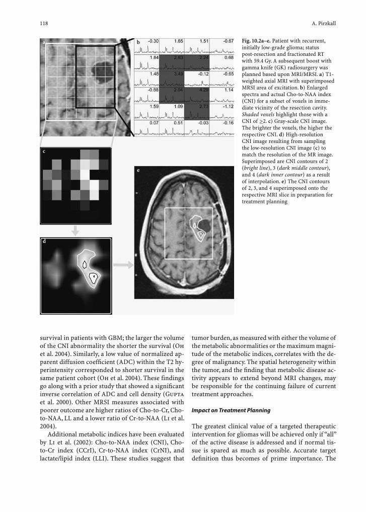
118 A. Pirzkall

survival in patients with GBM; the larger the volume of the CNI abnormality the shorter the survival (Oh et al. 2004). Similarly, a low value of normalized ap-parent diffusion coeffi cient (ADC) within the T2 hy-perintensity corresponded to shorter survival in the same patient cohort (Oh et al. 2004). These findings go along with a prior study that showed a signifi cant inverse correlation of ADC and cell density (Gupta et al. 2000). Other MRSI measures associated with poorer outcome are higher ratios of Cho-to-Cr, Cho-to-NAA, LL and a lower ratio of Cr-to-NAA (Li et al. 2004).

Additional metabolic indices have been evaluated by Li et al. (2002): Cho-to-NAA index (CNI), Cho-to-Cr index (CCrI), Cr-to-NAA index (CrNI), and lactate/lipid index (LLI). These studies suggest that

tumor burden, as measured with either the volume of the metabolic abnormalities or the maximum magni-tude of the metabolic indices, correlates with the de-gree of malignancy. The spatial heterogeneity within the tumor, and the fi nding that metabolic disease ac-tivity appears to extend beyond MRI changes, may be responsible for the continuing failure of current treatment approaches.

Impact on Treatment Planning

The greatest clinical value of a targeted therapeutic intervention for gliomas will be achieved only if “all” of the active disease is addressed and if normal tis-sue is spared as much as possible. Accurate target defi nition thus becomes of prime importance. The

Fig. 10.2a–e. Patient with recurrent, initially low-grade glioma; status post-resection and fractionated RT with 59.4 Gy. A subsequent boost with gamma knife (GK) radiosurgery was planned based upon MRI/MRSI. a) T1-weighted axial MRI with superimposed MRSI area of excitation. b) Enlarged spectra and actual Cho-to-NAA index (CNI) for a subset of voxels in imme-diate vicinity of the resection cavity. Shaded voxels highlight those with a CNI of >2. c) Gray-scale CNI image. The brighter the voxels, the higher the respective CNI. d) High-resolution CNI image resulting from sampling the low-resolution CNI image (c) to match the resolution of the MR image. Superimposed are CNI contours of 2 (bright line), 3 (dark middle contour), and 4 (dark inner contour) as a result of interpolation. e) The CNI contours of 2, 3, and 4 superimposed onto the respective MRI slice in preparation for treatment planning

ba

c

e

d

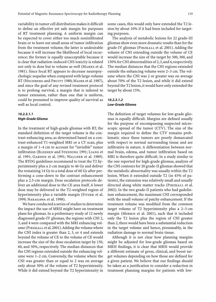
Potential of Magnetic Resonance Spectroscopy for Radiotherapy Planning 119

variability in tumor cell distribution makes it diffi cult to defi ne an effective yet safe margin for purposes of RT treatment planning. A uniform margin can be expected to cover either too much noninfi ltrated brain or to leave out small areas of tumor infi ltration from the treatment volume; the latter is undesirable because it will increase the likelihood of local recur-rence; the former is equally unacceptable because it is clear that radiation-induced CNS toxicity is related not only to dose but to volume as well (Marks et al. 1981). Since focal RT appears to decrease neuropsy-chologic sequelae when compared with large-volume RT (Hochberg and Pruitt 1980; Maire et al. 1987), and since the goal of any revised treatment protocol is to prolong survival, a margin that is tailored to tumor extension, rather than one that is uniform, could be presumed to improve quality of survival as well as local control.

10.2.3.1.1 High-Grade Glioma

In the treatment of high-grade gliomas with RT, the standard defi nition of the target volume is the con-trast-enhancing area, as determined based on a con-trast-enhanced T1-weighted MRI or a CT scan, plus a margin of 1–4 cm to account for “invisible” tumor infi ltration (Bleehen and Stenning 1991; Liang et al. 1991; Garden et al. 1991; Wallner et al. 1989). The RTOG guidelines recommend to treat the T2 hy-perintensity plus a 2-cm margin to 46 Gy and deliver the remaining 14 Gy to a total dose of 60 Gy after per-forming a cone-down to the contrast enhancement plus a 2.5-cm margin. Dose escalation protocols de-liver an additional dose to the CE area itself. A lower dose may be delivered to the T2-weighted region of hyperintensity plus a variable margin (Fitzek et al. 1999; Nakagawa et al. 1998).

We have conducted a series of studies to determine the impact the use of MRSI might have on treatment plans for gliomas. In a preliminary study of 12 newly diagnosed grade-IV gliomas, the regions with CNI 2, 3, and 4 were compared with the MRI enhancing vol-ume (Pirzkall et al. 2001). Adding the volume where the CNI index is greater than 2, 3, or 4 and extends beyond the volume of CE to the volume of CE would increase the size of the dose escalation target by 150, 60, and 50%, respectively. The median distances that the CNI regions extended outside the enhancing vol-ume were 1–2 cm. Conversely, the volume where the CNI was greater than or equal to 2 was on average only about 50% of the volume of T2 hyperintensity. While it did extend beyond the T2 hyperintensity in

some cases, this would only have extended the T2 le-sion by about 10% if it had been included for target-ing purposes.

The analysis of metabolic lesions for 22 grade-III gliomas show even more dramatic results than for the grade-IV gliomas (Pirzkall et al. 2001). Adding the volume of CNI extending outside the volume of CE would increase the size of the target by 500, 300, and 150% for CNI abnormalities of 2, 3, and 4, respectively. The median distances that the CNI regions extended outside the enhancing volume were 2–3 cm. The vol-ume where the CNI was 2 or greater was on average about 70% of the T2 lesion, and while it did extend beyond the T2 lesion, it would have only extended the target by about 15%.

10.2.3.1.2 Low-Grade Glioma

The defi nition of target volumes for low-grade glio-mas is equally diffi cult. Margins are defi ned usually for the purpose of encompassing suspected micro-scopic spread of the tumor (CTV). The size of the margin required to defi ne the CTV remains prob-lematic since these tumors are poorly demarcated with respect to normal surrounding tissue and are infi ltrative in nature. A differentiation between nor-mal brain, edema, and tumor infi ltration based on MRI is therefore quite diffi cult. In a study similar to the one reported for high-grade gliomas, analysis of the CNI contours for 20 grade-II gliomas showed that the metabolic abnormality was usually within the T2 lesion. When it extended outside T2 (in 45% of pa-tients), the extension was relatively small and usually directed along white matter tracks (Pirzkall et al. 2002). In the two grade-II patients who had gadolin-ium enhancement, the maximum CNI corresponded with the small volume of patchy enhancement. If the treatment volume was modifi ed from the common target volume of T2 hyperintensity plus a 2–3 cm margin (Morris et al. 2001), such that it included only the T2 lesion plus the region of CNI greater than 2, there would have been a substantial reduction in the target volume and hence, presumably, in the radiation damage to normal brain tissue.

Although it is not clear how planning margins might be adjusted for low-grade gliomas based on MRSI fi ndings, it is clear that MRSI would provide a different estimate of gross, clinical, and boost tar-get volumes depending on how those are defi ned for a given patient. We believe that our fi ndings should be taken as a justifi cation to consider a reduction in treatment planning margins for patients with low-

120 A. Pirzkall

grade glioma, paying careful attention to preferential avenues of spread of disease. It is also interesting to note that even low-grade gliomas demonstrate re-gions of varying metabolic activity within their vol-ume. The possible differentiation of more or less ra-diosensitive/resistant areas, as defi ned by metabolic measures, may play an important role in the future diagnosis and treatment of low-grade gliomas.

In addition to being of value in determining the overall volume appropriate for treatment, the meta-bolic heterogeneity defi ned by MRSI might be of particular interest when deciding on “differential” therapy to delineated regions within brain gliomas. MRSI might offer valuable information on the rela-tive radiosensitivity or radioresistence of certain tissue types within a neoplastic lesion and thus on desired dose. For instance, the presence of lactate can be considered an indicator of anaerobic metabolism, suggestive of poor blood supply and therefore the presence of hypoxic cells within the tumor. Targeting these areas with focal higher doses may be appropri-ate. In contrast, regions with increased Cr relative to NAA refl ect high cellularity and active bioenergetic processes (phosphorylation of ADP); therefore, re-gions of tumor with a CrNI >2 may indicate radio-sensitive areas that might be adequately treated with a lower dose.

10.2.3.2 Radiosurgery for Recurrent Gliomas

The idea of combining IMRT and MRSI data to de-liver extremely sophisticated treatment plans with differential doses delivered across the target volume is still quite “theoretical” for the treatment of brain gliomas; however, its value in radiosurgery (RS) for recurrent malignant gliomas has a stronger bias. Although the prognosis for recurrent gliomas is poor in general, focal re-treatment has been shown to prolong survival. Radiosurgery, although seem-ingly counterintuitive for an infi ltrating disease such as recurrent gliomas, offers an effective and nonin-vasive treatment option, with median survival times after radiosurgery for grade-IV gliomas in the order of 8–13 months (Chamberlain et al. 1994; Hall et al. 1995; Larson et al. 1996). Recurrence patterns, however, are predominantly local and marginal in up to 80% (Hall et al. 1995; Shrieve et al. 1995).

Graves et al. (2000) studied the prognostic value of MRSI in gamma knife (GK) RS of recurrent ma-lignant gliomas. Thirty-six patients with recurrent gliomas were retrospectively divided into two groups depending on whether the metabolic lesion was con-

fi ned to the radiosurgical target or whether it ex-tended well outside the target. Among the patients with recurrent GBM, the most signifi cant fi nding was a poorer median survival of 36 weeks in patients with metabolic extension vs 96 weeks for patients with no metabolic abnormality beyond the radiosurgical tar-get at the time of treatment. In addition, a signifi cant difference was found between the two groups in the volume of CE as assessed throughout the follow-up period, with an increase in CE in the patient group with metabolic abnormality beyond the region of treatment. In some cases the metabolic lesion outside the treatment area would have been small enough to be included within the GK target, but in others the lesion would have been too large to be treated ad-equately. A more recent study by Chan et al. (2004) employed the Cho-to-NAA Index (CNI) to examine the degree of overlap between the radiosurgically treated volume and the volume where the CNI was greater than or equal to 2. Based on degree of overlap, patients were divided into two risk groups and it was found that the survival for the low-risk group was signifi cantly longer than for the high-risk group.

This analysis prompted us to look at the poten-tial impact that MRSI would have on patient selec-tion and treatment plans for RS of recurrent gliomas (Pirzkall et al. 2001). In 18 patients with recurrent glioma (4 anaplastic astrocytomas and 14 GBM) treated with GK at UCSF, the radiosurgical target vol-ume (contrast enhancement plus 1–2 mm) was com-pared with the CNI volumes derived from the prior to GK acquired MRSI as described above. The CNI abnormality was found to extend beyond the CE to some degree in all patients. This extension was signif-icant (>6 cc) in 11 of 18 patients (61%). In 4 of these 11 patients, the metabolic abnormality was com-pletely outside the CE. If adding the CNI abnormality to the volume of contrast enhancement, the standard target volume would increase by 9–277% (0.5–27 cc). Such target defi nition would require a change in the dose prescription according to the GK dose-volume relationship in 12 of 18 patients (67%). In fact, 4 pa-tients (22%) would have had a treatment volume ex-ceeding 20 cc and would therefore not be considered eligible for RS in most institutions.

As an extension to this study, we are currently ex-amining the follow-up studies in patients who exhib-ited metabolic activity beyond the volume of contrast enhancement that remained outside the radiosurgical target volume in order to assess recurrence patterns. These data are now available (Chuang et al. 2004).

We are also developing an institutional protocol that will investigate the incorporation of CNI con-

Potential of Magnetic Resonance Spectroscopy for Radiotherapy Planning 121

tours into the selection process and the target defi -nition for RS (see Fig. 10.3), where appropriate (e.g. noneloquent brain regions), and will implement a phase-I study that will assess toxicity of such ap-proach.

10.2.3.3 Treatment Protocol for Newly Diagnosed GBM

Combining metabolic imaging guidance by means of MRSI (and proton-weighted MR, diffusion-weighted MR) with the powerful capability of IMRT to increase dose selectively while simultaneously prescribing a conventional-like dose to areas at lower risk has been the goal of our group for several years. We have tested the feasibility of incorporating MRSI data into the IMRT treatment planning process and established the necessary image data analysis and transfer (Graves et al. 2001; Nelson et al. 2002). We previously discussed the possibility of defi ning the GTV or boost volume according to the contrast enhancement enlarged by the CNI abnormality and

the CTV according to the T2 hyperintensity plus the CNI, a proposal that seemed reasonable based on the assumption that the CNI correlates with cell den-sity. This latter fact has been confi rmed for grade-III gliomas (McKnight et al. 2002) but is currently still under investigation for GBM samples. Recent stud-ies have suggested that the use of CNI abnormalities to enlarge the defi nition of the GTV may not be the optimal approach. These studies showed that the ad-dition of CNI abnormality to the volume of contrast enhancement would increase its average volume by 60% (CNI >3) and 50% (CNI >4), if the contrast en-hancement alone would have been defi ned (Pirzkall et al. 2001). In addition, preliminary patterns of re-currence analysis in presumed gross totally resected GBM after conventional RT with 60 Gy indicate that the fi rst onset of new contrast enhancement during follow-up was contained within the overall extent of pre-RT metabolic abnormality (CNI 2) in 7 of 8 pa-tients (Pirzkall et al. 2004), but even the volumes of CNI greater than or equal to 3 or 4 were still much larger than the volume of new contrast enhancement

Fig. 10.3. Same case as in Fig. 10.2. Upper row: GK treat-ment plan for the respective case in axial and sagittal plane. The inner dark line shows the radiosurgical target that encompasses the resec-tion cavity and tumor-sug-gestive areas according to the CNI. Isodose lines (IDL) of 50 (prescription IDL), 25, and 12.5%, respectively, are shown as brighter lines surround-ing the target (from inside to outside). Bottom row: Follow-up MRI at 4 months post-GK shows contrast enhancement particularly in the medio-posterior and superior aspect worrisome of tumor recur-rence. Continued increase in contrast enhancement over the subsequent 2 months prompted a re-resection. Histopathology revealed glio-sis and necrotic tissue com-patible with radiation effect

122 A. Pirzkall

at fi rst onset. This suggests that the volume of CNI 3 and 4 would be too generous for many patients. Correlation to other metabolic indices, such as CrNI, CCrI, and LL, did not reveal a uniform pattern either. Further evaluation of recurrence patterns in this pa-tient group is currently ongoing based on a larger patient population with the addition of new pulse sequences so that lactate and lipid resonances can be separated for improved interpretation.

Another obstacle that still needs to be addressed is extending the coverage of the tumor and sur-rounding areas while maintaining suffi cient cover-age of normal-appearing brain tissue. This is part of a technical development effort that will be under-taken shortly. Once these limitations are addressed, a clinical phase-I study that uses metabolic imaging-enhanced target defi nition and dose prescription by means of IMRT will be initiated for newly diagnosed patients with GBM.

10.2.3.4 Assessing Response to RT

The interpretation of MRI changes following RT con-tinues to pose a problem for all clinicians who are trying to decide whether a tumor has recurred and needs additional treatment. A continuous increase in contrast enhancement of more than 25% has been considered by most protocols as a benchmark for assessing tumor recurrence. In more recent studies, additional MR parameters are being looked at, in-cluding MRSI, as well as perfusion- and diffusion-weighted MRI.

Several groups are currently investigating the value of MRSI for assessing response to RT. Patients found to respond to therapy have been reported as showing a reduction in Cho, whereas patients who progressed exhibit a retention or increase in Cho (Wald et al. 1997; Taylor et al. 1996; Sijens et al. 1995). Another indicator of therapy response is the occurrence or increase in the Lac/Lip peak. Those changes have to be interpreted in light of changes in normal tissue as well. Virta (2000) et al. describe transient reductions in NAA and relative increases in Cho in normal-appearing white matter following RT. Late effects of radiation were studied by Esteve et al. (1998) who reports on reductions in Cho, Cr, and NAA in regions of T2 hyperintensity and reductions in Cho in normal-appearing white matter. Lee et al. (2004) tried to quantify the dose dependent effect in normal tissue post RT. The Cho-to-NAA ratio for in-stance, exhibited its steepest dose-dependent increase to 117–125% of its original value by 2 months post-

RT and underwent a dose-dependent recovery later on but did not return to its original value within the 6 month follow-up. A similar trend in the Cho-to-Cr ratio and separate metabolite analyses suggested that Cho underwent the most signifi cant changes. These normal tissue changes have to be taken into account when trying to assess tumor response to therapy.

10.2.4 Prostate

General

Modern RT delivers doses of more far more than 70 Gy in patients with T1–T3 prostate in response to fi ndings of (a) increased biopsy-proven local recur-rences after CRT of 70 Gy and less (Crook et al. 1995), and (b) decreased probability of relapse with increas-ing doses (Pollack and Zagars 1997). Three-di-mensional CRT and IMRT have been employed as a means to escalate dose.

Zelefsky et al. (2001) propose to treat localized prostate cancer with 81 Gy claiming superior control and decreased toxicity if treated with IMRT based on preliminary data. Even though it remains to be seen whether the shapes of the dose-response curve and complication-probability curves justify doses above 75.6 Gy, being able to direct/intensify dose at the area of highest risk appears benefi cial.

On T2-weighted MRI, regions of cancer within the prostate demonstrate lower signal intensity relative to healthy peripheral zone tissue as a result of loss of normal ductal morphology and associated long T2 water signal. Efforts to identify the location of tumor within the prostate have included digital rectal exam-ination, prostate-specifi c antigen (PSA), PSA density, systematic biopsy, transrectal ultrasound (TRUS), and MRI, but none of those have provided satisfying results for disease targeted therapies.

Recent studies in pre-prostatectomy patients have indicated that the metabolic information provided by MRSI combined with the anatomical informa-tion provided by MRI can signifi cantly improve the assessment of cancer location and extent of disease within the prostate, the magnitude of extracapsular spread, and the degree of cancer aggressiveness. The MRI alone has good sensitivity (78%) but low speci-fi city (55%) in identifying the tumor location within the prostate because of a large number of false posi-tives attributable to noncancerous changes such as post-biopsy hemorrhage, prostatitis, and therapeutic effects (Hricak et al. 1994). The addition of MRSI

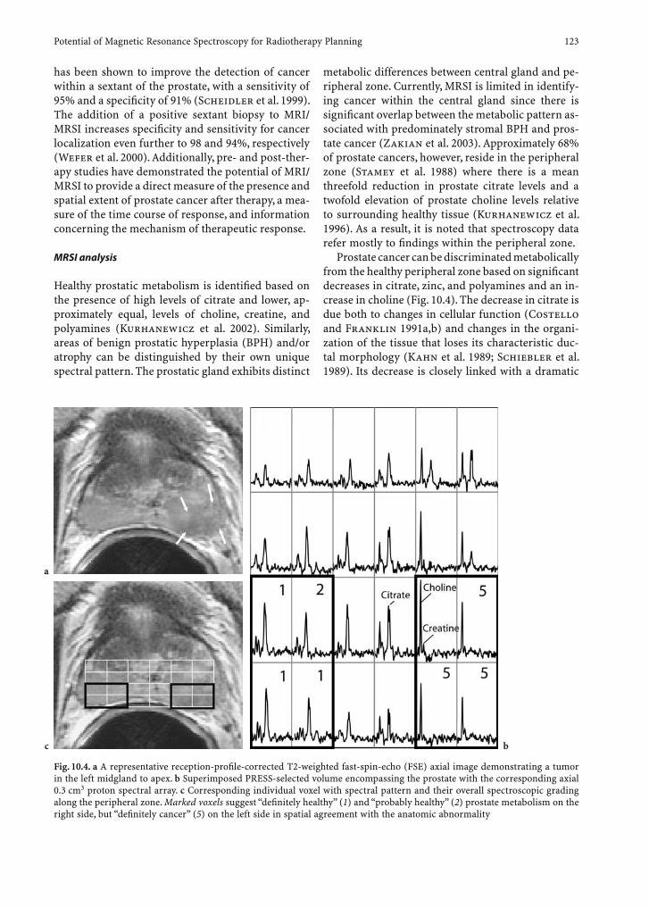
Potential of Magnetic Resonance Spectroscopy for Radiotherapy Planning 123

has been shown to improve the detection of cancer within a sextant of the prostate, with a sensitivity of 95% and a specifi city of 91% (Scheidler et al. 1999). The addition of a positive sextant biopsy to MRI/MRSI increases specifi city and sensitivity for cancer localization even further to 98 and 94%, respectively (Wefer et al. 2000). Additionally, pre- and post-ther-apy studies have demonstrated the potential of MRI/MRSI to provide a direct measure of the presence and spatial extent of prostate cancer after therapy, a mea-sure of the time course of response, and information concerning the mechanism of therapeutic response.

MRSI analysis

Healthy prostatic metabolism is identifi ed based on the presence of high levels of citrate and lower, ap-proximately equal, levels of choline, creatine, and polyamines (Kurhanewicz et al. 2002). Similarly, areas of benign prostatic hyperplasia (BPH) and/or atrophy can be distinguished by their own unique spectral pattern. The prostatic gland exhibits distinct

metabolic differences between central gland and pe-ripheral zone. Currently, MRSI is limited in identify-ing cancer within the central gland since there is signifi cant overlap between the metabolic pattern as-sociated with predominately stromal BPH and pros-tate cancer (Zakian et al. 2003). Approximately 68% of prostate cancers, however, reside in the peripheral zone (Stamey et al. 1988) where there is a mean threefold reduction in prostate citrate levels and a twofold elevation of prostate choline levels relative to surrounding healthy tissue (Kurhanewicz et al. 1996). As a result, it is noted that spectroscopy data refer mostly to fi ndings within the peripheral zone.

Prostate cancer can be discriminated metabolically from the healthy peripheral zone based on signifi cant decreases in citrate, zinc, and polyamines and an in-crease in choline (Fig. 10.4). The decrease in citrate is due both to changes in cellular function (Costello and Franklin 1991a,b) and changes in the organi-zation of the tissue that loses its characteristic duc-tal morphology (Kahn et al. 1989; Schiebler et al. 1989). Its decrease is closely linked with a dramatic

Fig. 10.4. a A representative reception-profi le-corrected T2-weighted fast-spin-echo (FSE) axial image demonstrating a tumor in the left midgland to apex. b Superimposed PRESS-selected volume encompassing the prostate with the corresponding axial 0.3 cm3 proton spectral array. c Corresponding individual voxel with spectral pattern and their overall spectroscopic grading along the peripheral zone. Marked voxels suggest “defi nitely healthy” (1) and “probably healthy” (2) prostate metabolism on the right side, but “defi nitely cancer” (5) on the left side in spatial agreement with the anatomic abnormality

b

a

c

124 A. Pirzkall

reduction of zinc levels, an important factor in the transformation of prostate epithelial cells to citrate oxidizing cells and the development and progression of prostate cancer. The elevation in Cho is associ-ated with changes in cell membrane synthesis and degradation that occur with the evolution of human cancers (Aboagye and Bhujwalla 1999). The poly-amines spermin, spermidine, and putrescine are also abundant in healthy prostatic tissues and reduced in cancer. Polyamines have been associated with cellu-lar differentiation and proliferation (Heston 1991).

In order to quantify spectral metabolites in the pe-ripheral zone a standardized fi ve-point scale has been developed (Jung et al. 2004). A score from 1 to 5 is as-signed to each spectroscopic voxel based on changes in choline, citrate, and polyamines (Fig. 10.4). A score of 1 is considered to be defi nitely benign, 2 likely be-nign, 3 equivocal, 4 likely abnormal, and 5 defi nitely abnormal. Regions of three or more adjacent abnor-mal spectroscopic voxels with scores of 4 and/or 5 that show a correspondence with anatomic abnor-mality (decreased signal intensity on T2-weighted images) are read as cancer and are termed “dominant intraprostatic lesion” (DIL).

Tumor Analysis

Knowledge of possible cancer spread outside the prostate is critical for choosing the appropriate therapy. Endorectal MRI has an excellent negative predictive value for detecting seminal vesicle inva-sion (d’Amico et al. 1998) but is less accurate in the assessment of extracapsular extension. This assess-ment can be signifi cantly improved by combining MRI fi ndings that are predictive of cancer spread with an estimate of the spatial extent of metabolic ab-normality as assessed by MRSI (Yu et al. 1999); MRSI-derived tumor volume per lobe was signifi cantly higher in patients with extracapsular extension than in patients without. Preliminary MRI/MRSI biopsy correlation studies also have shown that increased levels of choline and decreased levels of citrate cor-relate with the degree of pathology as measured by the Gleason score (Vigneron et al. 1998). Targeted postsurgical prostate tissue samples studied spectro-scopically ex vivo have confi rmed such a correlation (Swanson et al. 2003).

Impact on Treatment Planning

The described capability of combined MRI/MRSI to localize intraglandular cancer, evaluate extracapsular extent of the disease, and grade cancer aggressiveness

makes it of value not only for patient selection but also for disease-targeted treatments such as cryo-surgery, high-intensity ultrasonography (HIFU), and especially focal RT. One motivation for incorporating MRI/MRSI into the treatment planning process for RT is that the noncontrast enhanced CT overesti-mates the volume of the prostate as compared with MRI, is inadequate in identifying the complex anat-omy of the prostate (Roach et al. 1996), and sheds no light on identifying those areas that might benefi t from increased dose. The integration of MRI/MRSI information into the treatment plan can be used to optimize dose planning and reduce the dose deliv-ered to surrounding organs at risk (rectum, bladder, neurovascular bundles, etc.) and hence decrease the incidence of damage to normal tissues. Perhaps more importantly, the MRI/MRSI/biopsy-identifi ed DILs can be targeted with increased dose with the hope of increased tumor control and, at the same time, a po-tential decrease in overall treatment time if increased daily dose fractions could be applied safely.

Prostate cancer is usually a multifocal disease and, therefore, most patients have multiple DILs. Delivering a high dose uniformly to the entire pros-tate increases the risk of complications to surround-ing normal tissues. Selective dose intensifi cation techniques to the spectroscopically identifi ed DIL(s) seems appropriate, thereby targeting the area of cancer with increased dose. Such a treatment ratio-nale has been pursued at UCSF to date. Approaches have included: (a) static fi eld IMRT (SF-IMRT); (b) forward planned segmental multileaf collima-tion (SMLC) IMRT (Pickett et al. 1999); (c) inverse planned SMLC or sequential tomotherapy employing the MIMiC collimator (Xia et al. 2001); (d) inverse planned radiosurgical boost IMRT (Pickett et al. 2000); (e) brachytherapy via radioactive iodine-125 seed implantation (Pickett et al. 2004) or high-dose rate application (Pouliot et a. 2004).

In order to incorporate the spectral information into the treatment planning process for RT, MRI/MRSI data have to be co-registered to the treatment plan-ning CT; however, one confounding factor in merging these data sets is the distortion of the prostate by the infl atable rectal coil. As expected, a comparison of the anatomy derived from CT with and without the en-dorectal coil has demonstrated substantial displace-ment differences when the endorectal coil was used (Vigneault et al. 1997). The acquisition of images with and without the endorectal coil within the same exam improves the translation of the MRSI data to the nondistorted images for manual merging with the planning CT or MRI scans (Pouliot et al. 2004).

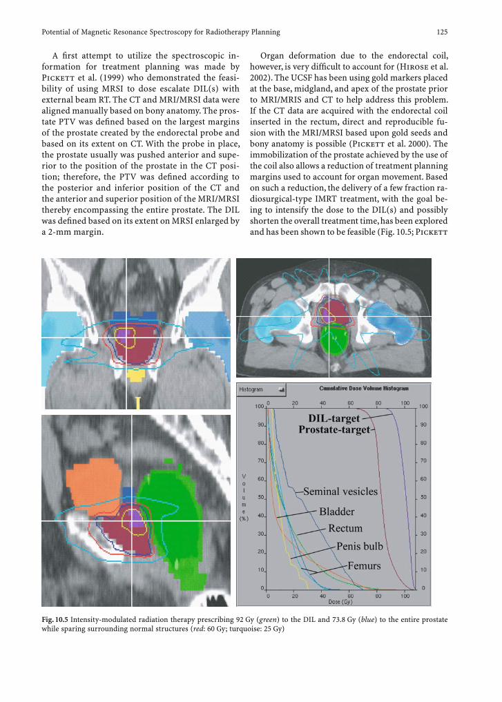
Potential of Magnetic Resonance Spectroscopy for Radiotherapy Planning 125

A fi rst attempt to utilize the spectroscopic in-formation for treatment planning was made by Pickett et al. (1999) who demonstrated the feasi-bility of using MRSI to dose escalate DIL(s) with external beam RT. The CT and MRI/MRSI data were aligned manually based on bony anatomy. The pros-tate PTV was defi ned based on the largest margins of the prostate created by the endorectal probe and based on its extent on CT. With the probe in place, the prostate usually was pushed anterior and supe-rior to the position of the prostate in the CT posi-tion; therefore, the PTV was defi ned according to the posterior and inferior position of the CT and the anterior and superior position of the MRI/MRSI thereby encompassing the entire prostate. The DIL was defi ned based on its extent on MRSI enlarged by a 2-mm margin.

Organ deformation due to the endorectal coil, however, is very diffi cult to account for (Hirose et al. 2002). The UCSF has been using gold markers placed at the base, midgland, and apex of the prostate prior to MRI/MRIS and CT to help address this problem. If the CT data are acquired with the endorectal coil inserted in the rectum, direct and reproducible fu-sion with the MRI/MRSI based upon gold seeds and bony anatomy is possible (Pickett et al. 2000). The immobilization of the prostate achieved by the use of the coil also allows a reduction of treatment planning margins used to account for organ movement. Based on such a reduction, the delivery of a few fraction ra-diosurgical-type IMRT treatment, with the goal be-ing to intensify the dose to the DIL(s) and possibly shorten the overall treatment time, has been explored and has been shown to be feasible (Fig. 10.5; Pickett

Fig. 10.5 Intensity-modulated radiation therapy prescribing 92 Gy (green) to the DIL and 73.8 Gy (blue) to the entire prostate while sparing surrounding normal structures (red: 60 Gy; turquoise: 25 Gy)

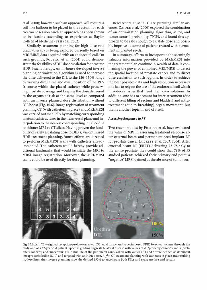
126 A. Pirzkall

et al. 2000); however, such an approach will require a coil-like balloon to be placed in the rectum for each treatment session. Such an approach has been shown to be feasible according to experience at Baylor College of Medicine (Teh et al. 2002).

Similarly, treatment planning for high-dose rate brachytherapy is being explored currently based on MRI/MRSI data acquired with an endorectal coil. On such grounds, Pouliot et al. (2004) could demon-strate the feasibility of DIL dose escalation for prostate HDR Brachytherapy. An in-house developed inverse planning optimization algorithm is used to increase the dose delivered to the DIL to the 120–150% range by varying dwell time and dwell position of the 192-Ir source within the placed catheter while preserv-ing prostate coverage and keeping the dose delivered to the organs at risk at the same level as compared with an inverse planned dose distribution without DIL boost (Fig. 10.6). Image registration of treatment planning CT (with catheters in place) and MRI/MRSI was carried out manually by matching corresponding anatomical structures in the transversal plane and in-terpolation to the nearest corresponding CT slice due to thinner MRI vs CT slices. Having proven the feasi-bility of safely escalating dose to DIL(s) via optimized HDR treatment planning, future efforts are directed to perform MRI/MRSI scans with catheters already implanted. The catheters would hereby provide ad-ditional landmarks that would facilitate the MRI to MRSI image registration. Moreover, the MRI/MRSI scans could be used directly for dose planning.

Researchers at MSKCC are pursuing similar av-enues. Zaider et al. (2000) explored the combination of an optimization planning algorithm, MRSI, and tumor control probability (TCP), and found this ap-proach to be safe enough to escalate dose and possi-bly improve outcome of patients treated with perma-nent implanted seeds.

In summary, efforts to incorporate the seemingly valuable information provided by MRI/MRSI into the treatment plan continue. A wealth of data is con-fi rming the power of combined MRI/MRSI to detect the spatial location of prostate cancer and to direct dose escalation to such regions. In order to achieve the best possible data and high resolution necessary one has to rely on the use of the endorectal coil which introduces issues that need their own solutions. In addition, one has to account for inter-treatment (due to different fi lling of rectum and bladder) and intra-treatment (due to breathing) organ movement. But that is another topic in and of itself.

Assessing Response to RT

Two recent studies by Pickett et al. have evaluated the value of MRI in assessing treatment response af-ter external beam and permanent seed implant RT for prostate cancer (Pickett et al. 2003, 2004). After external beam RT (EBRT) delivering 72–75.6 Gy to the entire prostate, they could show that 78% of 55 studied patients achieved their primary end point, a “negative” MRSI defi ned as the absence of tumor sus-

Fig. 10.6 Left: T2-weighted reception-profi le-corrected FSE axial image and superimposed PRESS-excited volume through the midgland of a 67-year-old patient. Spectral grading suggests bilateral disease with values of 4 (“probably cancer”) and 5 (“defi -nitely cancer”) and “uncertain” (3) in midline of the peripheral zone. Voxels with values of 4 and 5 were defi ned as dominant intraprostatic lesion (DIL) and targeted with an HDR boost. Right: CT treatment planning with catheters in place and resulting isodose lines after inverse planning show the desired 150% to encompass both DILs and spare urethra and rectum

Potential of Magnetic Resonance Spectroscopy for Radiotherapy Planning 127

picious spectra, at various time points >26 months post-RT (Pickett et al. 2003). The time course of response is hereby of interest: the percent of voxels indicating metabolic atrophy increased from 76% at 18 months to 93% at 55 months post-RT. Mean over-all time to resolution of disease was 40 months. The MRSI revealed persistent cancerous metabolism in 22% of patients at the end of evaluation and are re-ferred to biopsy if still persistent at 36 months post-EBRT.

After permanent prostate implant (PPI), on the other hand, MRSI exams suggested complete meta-bolic atrophy in 46% of 65 examined patients at 6 months post-PPI and, after continued follow-up, in all patients by 48 months after PPI (Pickett et al. 2004). Complete metabolic atrophy was seen in only 31% of the patients treated with EBRT. This dramatic difference in treatment response and its time course is likely attributable to the signifi cantly higher pre-scribed dose (144 Gy PPI vs 70–75.6 Gy EBRT). In addition, both studies found that MRSI seemed to indicate therapeutic effectiveness much earlier than the PSA level reached its nadir. It was concluded that the MRSI-derived time to metabolic atrophy appears to be a very useful adjunct to PSA for assessing local control following PPI.

In a study of 21 patients with biochemical failure after external-beam radiation therapy for prostate cancer in whom subsequent biopsy confi rmed lo-cally recurrent prostate cancer, Coakley et al. (2004) found that the presence of three or more MRSI vox-els with isolated elevated choline to creatine (ratio greater than 1.5) showed a sensitivity and specifi city of 87 and 72%, respectively. This preliminary study suggests that MRSI may have a role in detecting local cancer recurrence post-radiation.

10.3 Current Limitations and Possible Solutions

Developing MRSI as a tool for routine use for brain tumors with respect to radiation therapy planning and follow-up requires improvements in coverage of the lesion and in the signal-to-noise ratio of the spectral data. The spectroscopy studies performed at our institution have been restricted to a rectangular area of excitation (PRESS box) that is of limited vol-ume. Since gliomas are relatively large and irregular in shape, this means that in many cases we have not covered the entire lesion. The volume limitation is a function of the signal-to-noise ratio and acquisition

time for a given spatial resolution. Our current stud-ies have limited the MRSI acquisition time to 17 min so that the entire exam can be performed in conjunc-tion with a conventional MRI exam.

Optimization of the methods for lipid suppression are critical for achieving adequate coverage of the an-atomic lesion and surrounding normal tissue with-out compromising spectral quality. Very selective sat-uration bands (VSS) have been used to sharpen the edges of the PRESS volume and to suppress regions of subcutaneous lipid and bone on the edges of the selected volume. Future studies will examine alterna-tive combinations of VSS pulses, as well as balancing the trade-off between increased imaging time and data quality. This will also be improved by utilizing a higher-strength magnet or improved radiofrequency coils.

There is also a need for further development con-cerning the calculation of metabolic indices; these are currently generated from the data that have a nominal spatial resolution of 1 cc and results in po-tentially large partial-volume effects. Higher spatial resolution can be achieved using surface or phased-array radiofrequency coils. Resolutions as small as 0.2 cc have been achieved for brain tumors and other focal lesions of the cortex at 1.5 T. Magnets as strong as 3–7 T will improve this capability even further. An additional benefi t of higher fi eld strengths is the improved spectral dispersion and increased T2 relax-ation times which will allow estimation of additional metabolites that are currently not being assessed.

One of the problems in the prostate is organ de-formation due to the use of infl ated rectal coils. A newly designed, noninfl atable, rigid endorectal coil for MRI/MRSI may reduce deformity of the prostate and the magnitude of the discrepancies between the prostate position on MRI/MRSI vs CT, making the data much more “transportable” for use in treatment planning.

Finally, it is not always clear how to interpret the metabolic data itself or which level of a metabolic in-dex should be used as a guide for defi ning a separate target or boost volume that should receive a higher or perhaps lower dose. Because of partial-volume ef-fects, a region of given metabolic index could have a few cells with very high metabolic activity and many cells with little activity and/or necrosis, or it could contain all cells with average activity. These two scenarios might suggest different therapeutic so-lutions. For instance, it seems intuitive that regions with greater metabolic activity (however that is de-fi ned) should be targeted for an integrated boost; however, it could also be argued that the regions with

128 A. Pirzkall

low metabolic activity are the ones that will require a greater dose of RT if poor oxygenation is causing such a state. Additional analysis of the MRSI metabo-lites discussed, as well as other metabolic data that may be acquired using advances in technique and instrumentation, may help in determining the re-quired analysis. MRI-based perfusion and diffusion-measuring techniques, such as cerebral blood volume (CBV) and apparent diffusion coeffi cient (ADC) for brain, and fast dynamic imaging, single-shot echo-planar (EPI)-based diffusion-weighted imaging, and single-shot fast spin echo/rapid acquisition with re-laxation enhancement (FSE/RARE) for prostate, may also help provide the differentiation required to bet-ter interpret the MRSI data.

10.4 Conclusion

MRSI has the potential to provide metabolic evidence of tumor activity that may be an important guide for therapeutic decisions. The treatment planning pro-cess and treatment planning systems should there-fore have the ability to incorporate both metabolic and anatomic data in order to determine appropriate target volumes. Many problems need to be addressed and much work needs to be done in order to deter-mine the optimal way to incorporate indices of meta-bolic activity, especially in light of newer treatment techniques such as IMRT; however, it is the present author’s belief that strong consideration should be given to the incorporation of functional imaging into the treatment process for focal or boost treatments for brain and prostate tumors. Given the discrepan-cies that have been found between MRI and MRSI de-terminants of target volumes, the results of controlled dose escalation studies for malignant tumors of the brain that have used MRI-derived target volumes should also be reevaluated given the possibility that these volumes may have been suboptimally defi ned.

Acknowledgements

I would like to thank the following colleagues for their support and helpful contributions to this chapter: S.J. Nelson, A.A. Chan, J.M. Lupo, M.C. Lee, E. Ozturk, F.W. Crawford, J. Oh, J. Kurhanewicz, C. Chuang, L.J. Verhey, B. Pickett, J. Pouliot, D.A. Larson, P.K. Sneed, S.M. Chang, M.W. McDermott, M.S. Berger, and M.P. Carol. This work was supported in part by NIH grants CA79719, CA 59880, and CA 97257.

References

Aboagye EO, Bhujwalla ZM (1999) Malignant transforma-tion alters membrane choline phospholipid metabolism of human mammary epithelial cells. Cancer Res 59:80–84

Bleehen NM, Stenning SP (1991) A Medical Research Council trial of two radiotherapy doses in the treatment of grades 3 and 4 astrocytoma. The Medical Research Council Brain Tumour Working Party. Br J Cancer 64:769–774

Burger PC, Heinz ER, Shibata T et al. (1988) Topographic anatomy and CT correlations in the untreated glioblastoma multiforme. J Neurosurg 68:698–704

Chamberlain MC, Barba D, Kormanik P et al. (1994) Stereo-tactic radiosurgery for recurrent gliomas. Cancer 74:1342–1347

Chan AA, Lau A, Pirzkall A et al. (2004) 1H-MRSI as a tool for evaluating grade IV glioma patients undergoing gamma knife radiosurgery. J Neurosurg 101:467–475

Chan JL, Lee SW, Fraass BA et al. (2002) Survival and failure patterns of high-grade gliomas after three-dimensional conformal radiotherapy. J Clin Oncol 20:1635–1642

Chuang C, Chan AA, Larson DL et al. (2004) Prognostic value of pre-Gamma Knife MR spectroscopic imaging for treat-ment strategy and clinical outcome. Int J Radiat Oncol Biol Phys (Abstract)

Coakley FV, Teh BS, Quayyum A et al. (2004) Endorectal MR and MR spectroscopic imaging of locally recurrent pros-tate cancer after external beam radiation therapy: prelimi-nary experience. Radiology 233:441–448

Costello LC, Franklin RB (1991a) Concepts of citrate produc-tion and secretion by prostate. 1. Metabolic relationships. Prostate 18:25–46

Costello LC, Franklin RB (1991b) Concepts of citrate produc-tion and secretion by prostate. 2. Hormonal relationships in normal and neoplastic prostate. Prostate 19:181–205

Crook JM, Perry GA, Robertson S et al. (1995) Routine prostate biopsies following radiotherapy for prostate cancer: results for 226 patients. Urology 45:624–631

D’Amico AV, Schnall M, Whittington R et al. (1998) Endorec-tal coil magnetic resonance imaging identifi es locally advanced prostate cancer in select patients with clinically localized disease. Urology 51:449–454

Esteve F, Rubin C, Grand S et al. (1998) Transient metabolic changes observed with proton MR spectroscopy in normal human brain after radiation therapy. Int J Radiat Oncol Biol Phys 40:279–286

Fitzek MM, Thornton AF, Rabinov JD et al. (1999) Acceler-ated fractionated proton/photon irradiation to 90 cobalt gray equivalent for glioblastoma multiforme: results of a phase II prospective trial. J Neurosurg 91:251–260

Garden AS, Maor MH, Yung WK et al. (1991) Outcome and patterns of failure following limited-volume irradiation for malignant astrocytomas. Radiother Oncol 20:99–110

Graves EE, Nelson SJ, Vigneron DB et al. (2000) A preliminary study of the prognostic value of proton magnetic reso-nance spectroscopic imaging in gamma knife radiosurgery of recurrent malignant gliomas. Neurosurgery 46:319–328

Graves EE, Pirzkall A, Nelson SJ et al. (2001) Registration of magnetic resonance spectroscopic imaging to computed tomography for radiotherapy treatment planning. Med Phys 28:2489–2496

Gupta RK, Cloughesy TF, Sinha U et al. (2000) Relationships between choline magnetic resonance spectroscopy, appar-

Potential of Magnetic Resonance Spectroscopy for Radiotherapy Planning 129

ent diffusion coeffi cient and quantitative histopathology in human glioma. J Neurooncol 50:215–226

Hall WA, Djalilian HR, Sperduto PW et al. (1995) Stereotactic radiosurgery for recurrent malignant gliomas. J Clin Oncol 13:1642–1648

Heston WD (1991) Prostatic polyamines and polyamine tar-geting as a new approach to therapy of prostatic cancer. Cancer Surv 11:217–238

Hirose M, Bharatha A, Hata N et al. (2002) Quantitative MR imaging assessment of prostate gland deformation before and during MR imaging-guided brachytherapy. Acad Radiol 9:906–912

Hochberg FH, Pruitt A (1980) Assumptions in the radiother-apy of glioblastoma. Neurology 30:907–911

Hricak H, White S, Vigneron D et al. (1994) Carcinoma of the prostate gland: MR imaging with pelvic phased-array coils versus integrated endorectal: pelvic phased-array coils. Radiology 193:703–709

Jung JA, Coakley FV, Quayyum A et al. (2004) Endorectal MR spectroscopi imaging of the prostate: investigation of a standardized evaluation system. Radiology 233:701–708

Kahn T, Burrig K, Schmitz-Drager B et al. (1989) Pros-tatic carcinoma and benign prostatic hyperplasia: MR imaging with histopathologic correlation. Radiology 173:847–851

Kelly PJ, Daumas-Duport C, Kispert DB et al. (1987) Imaging-based stereotaxic serial biopsies in untreated intracranial glial neoplasms. J Neurosurg 66:865–874

Kurhanewicz J, Swanson MG, Nelson SJ et al. (2002) Combined magnetic resonance imaging and spectroscopic imaging approach to molecular imaging of prostate cancer. J Magn Reson Imaging 16:451–463

Kurhanewicz J, Vigneron DB, Hricak H et al. (1996) Three-dimensional H-1 MR spectroscopic imaging of the in situ human prostate with high (0.24–0.7 cm3) spatial resolu-tion. Radiology 198:795–805

Kurhanewicz J, Vigneron DB, Nelson SJ (2000) Three-dimen-sional magnetic resonance spectroscopic imaging of brain and prostate cancer. Neoplasia 2:166–189

Larson DA, Gutin PH, McDermott M et al. (1996) Gamma knife for gliomas: selection factors and survival. Int J Radiat Oncol Biol Phys 36:1045–1053

Lee MC, Pirzkall A, McKnight TR et al. (2004) 1H-MRSI of radiation effects in normal-appearing white matter: dose-dependence and impact on automated spectral classifi ca-tion. J Magn Reson Imaging 19:379–388

Li X, Lu Y, Pirzkall A et al. (2002) Analysis of the spatial char-acteristics of metabolic abnormalities in newly diagnosed glioma patients. J Magn Reson Imaging 16:229–237

Li X, Jin H, Lu Y et al. (2004) Identifi cation of MRI and 1H MRSI parameters that may predict survival for patients with malignant gliomas. NMR Biomed 17:10–20

Liang BC, Thornton AF Jr, Sandler HM et al. (1991) Malignant astrocytomas: focal tumor recurrence after focal external beam radiation therapy. J Neurosurg 75:559–563

Maire JP, Coudin B, Guérin J et al. (1987) Neuropsychologic impairment in adults with brain tumors. Am J Clin Oncol 10:156–162

Marks JE, Baglan RJ, Prassad SC et al. (1981) Cerebral radione-crosis: incidence and risk in relation to dose, time, fraction-ation and volume. Int J Radiat Oncol Biol Phys 7:243–252

McKnight TR, Noworolski SM, Vigneron DB et al. (2001) An automated technique for the quantitative assessment of

3D-MRSI data from patients with glioma. J Magn Reson Imaging 13:167–177

McKnight TR, Bussche MH von dem, Vigneron DB et al. (2002a) Histopathological validation of a three-dimensional mag-netic resonance spectroscopy index as a predictor of tumor presence. J Neurosurg 97:794–802

McKnight TM, Vigneron DB, Love T et al. (2002b) Comparison of a Cho-NAA index with the MIB-1 proliferative index and cell density of tissue samples from grades II and III glioma. Proc 10th Scientifi c Meeting of the International Society of Magnetic Resonance in Medicine (ISMRM), Honolulu, Hawaii, p 43

Morris DE, Bourland JD, Rosenman JG et al. (2001) Three-dimensional conformal radiation treatment planning and delivery for low- and intermediate-grade gliomas. Semin Radiat Oncol 11:124–137

Nakagawa K, Aoki Y, Fujimaki T et al. (1998) High-dose con-formal radiotherapy infl uenced the pattern of failure but did not improve survival in glioblastoma multiforme. Int J Radiat Oncol Biol Phys 40:1141–1149

Nelson SJ (2001) Analysis of volume MRI and MR spectro-scopic imaging data for the evaluation of patients with brain tumors. Magn Reson Med 46:228–239

Nelson SJ, McKnight TR, Henry RG (2002a) Characterization of untreated gliomas by magnetic resonance spectroscopic imaging. Neuroimag Clin North Am 12:599–613

Nelson SJ, Graves E, Pirzkall A et al. (2002b) In vivo molecu-lar imaging for planning radiation therapy of gliomas: an application of 1H MRSI. J Magn Reson Imaging 16:464–476

Oh J, Henry RG, Pirzkall A et al. (2004) Survival analysis in patients with glioblastoma multiforme: predictive value of choline-to-N-acetylaspartate index, apparent diffusion coeffi cient, and relative cerebral blood volume. J Magn Reson Imaging 19:546–554

Pickett B, Vigneault E, Kurhanewicz J et al. (1999) Static fi eld intensity modulation to treat a dominant intra-prostatic lesion to 90 Gy compared to seven fi eld 3-dimensional radiotherapy. Int J Radiat Oncol Biol Phys 44:921–929

Pickett B, Pirzkall A, Kurhanewicz J et al. (2000) Radiosurgical intensity modulated radiotherapy for prostate cancer. Int J Radiat Oncol Biol Phys 48:S23

Pickett B, Kurhanewicz J, Fein B et al. (2003) Use of magnetic resonance imaging and spectroscopy in the evaluation of external beam radiation therapy for prostate cancer. Int J Radiat Oncol Biol Phys 57:S163–S164

Pickett B, TenHaken RK, Kurhanewicz J et al. (2004) Time course to metabolic atrophy following permanent prostate seed implantation based on magnetic resonance spectro-scopic imaging. Int J Radiat Oncol Biol Phys 59:665–673

Pirzkall A (2005) Magnetic resonance spectroscopy and its use in brain tumor diagnosis and therapy. In: Black P, Loeffl er JS (eds) Cancer of the nervous system, 2nd edn. Lippincott Williams and Wilkins, Philadelphia, pp 109–122

Pirzkall A, McKnight TR, Graves EE et al. (2001a) MR-spectros-copy guided target delineation for high-grade gliomas. Int J Radiat Oncol Biol Phys 50:915–928

Pirzkall A, Graves EE, Lau A et al. (2001b) Gamma knife (GK) radiosurgery (RS) for recurrent high-grade gliomas: What does magnetic resonance spectroscopy have to add? Fifth International Stereotactic Radiosurgery Society Congress (ISRS), Las Vegas, Nevada, p 44

Pirzkall A, Nelson SJ, McKnight TR et al. (2002) Metabolic

130 A. Pirzkall

imaging of low-grade gliomas with three-dimensional magnetic resonance spectroscopy. Int J Radiat Oncol Biol Phys 53:1254–1264

Pirzkall A, Li X, Oh J et al. (2004) 3D MRSI for resected high-grade gliomas before RT: tumor extent according to meta-bolic activity in relation to MRI. Int J Radiat Oncol Biol Phys 59:126–137

Pollack A, Zagars GK (1997) External beam radiotherapy dose response of prostate cancer. Int J Radiat Oncol Biol Phys 39:1011–1018

Pouliot J, Yongbok K, Lessard E et al. (2004) Inverse planning for HDR prostate brachytherapy use to boost dominant intraprostatic lesion defi ned by magnetic resonance spectro-scopic imaging. Int J Radiat Oncol Biol Phys 59:1196–1207

Roach M III, Faillace-Akazawa P, Malfatti C et al. (1996) Pros-tate volumes defi ned by magnetic resonance imaging and computerized tomographic scans for three-dimensional conformal radiotherapy. Int J Radiat Oncol Biol Phys 35:1011–1018

Scheidler J, Hricak H, Vigneron DB et al. (1999) Prostate cancer: localization with three-dimensional proton MR spectroscopic imaging: clinicopathologic study. Radiology 213:473–480

Schiebler ML, Tomaszewski JE, Bezzi M et al. (1989) Prostatic carcinoma and benign prostatic hyperplasia: correlation of high-resolution MR and histopathologic fi ndings. Radiol-ogy 172:131–137

Schricker AA, Pauly JM, Kurhanewicz J et al. (2001) Dualband spectral-spatial RF pulses for prostate MR spectroscopic imaging. Magn Reson Med 46:1079–1087

Shrieve DC, Alexander E III, Wen PY et al. (1995) Compari-son of stereotactic radiosurgery and brachytherapy in the treatment of recurrent glioblastoma multiforme. Neuro-surgery 36:275–282

Sijens PE, Vecht CJ, Levendag PC et al. (1995) Hydrogen mag-netic resonance spectroscopy follow-up after radiation therapy of human brain cancer. Unexpected inverse cor-relation between the changes in tumor choline level and post-gadolinium magnetic resonance imaging contrast. Invest Radiol 30:738–744

Sneed PK, Lamborn KR, Larson DA et al. (1996) Demonstra-tion of brachytherapy boost dose-response relationships in glioblastoma multiforme. Int J Radiat Oncol Biol Phys 35:37–44

Stamey TA, McNeal JE, Freiha FS et al. (1988) Morphometric and clinical studies on 68 consecutive radical prostatecto-mies. J Urol 139:1235–1241

Swanson MG, Vigneron DB, Tabatabai ZL et al. (2003) Proton HR-MAS spectroscopy and quantitative pathologic analy-sis of MRI/3D-MRSI-targeted postsurgical prostate tissues. Magn Reson Med 50:944–954

Taylor JS, Langston JW, Reddick WE et al. (1996) Clinical value of proton magnetic resonance spectroscopy for differenti-ating recurrent or residual brain tumor from delayed cere-

bral necrosis. Int J Radiat Oncol Biol Phys 36:1251–1261Teh BS, McGary JE, Dong L et al. (2002) The use of rectal bal-

loon during the delivery of intensity modulated radiother-apy (IMRT) for prostate cancer: More than just a prostate gland immobilization device? Cancer J 8:476–483

Thilmann C, Zabel A, Grosser KH et al. (2001) Intensity-modulated radiotherapy with an integrated boost to the macroscopic tumor volume in the treatment of high-grade gliomas. Int J Cancer 96:341–349

Tran TK, Vigneron DB, Sailasuta N et al. (2000) Very selective suppression pulses for clinical MRSI studies of brain and prostate cancer. Magn Reson Med 43:23–33

Vigneault E, Pouliot J, Laverdiere J et al. (1997) Electronic portal imaging device detection of radioopaque markers for the evaluation of prostate position during megavoltage irradiation: a clinical study. Int J Radiat Oncol Biol Phys 37:205–212

Vigneron DB, Males R, Hricak H et al. (1998) Prostate cancer: correlation of 3D MRSI metabolite levels with histologic grade. RSNA, Chicago, p 181

Virta A, Patronas N, Raman R et al. (2000) Spectroscopic imaging of radiation-induced effects in the white matter of glioma patients. Magn Reson Imaging 18:851–857

Wald LL, Nelson SJ, Day MR et al. (1997) Serial proton mag-netic resonance spectroscopy imaging of glioblastoma multiforme after brachytherapy. J Neurosurg 87:525–534

Wallner KE, Galicich JH, Krol G et al. (1989) Patterns of failure following treatment for glioblastoma multiforme and anaplastic astrocytoma. Int J Radiat Oncol Biol Phys 16:1405–1409

Wefer AE, Hricak H, Vigneron DB et al. (2000) Sextant local-ization of prostate cancer: comparison of sextant biopsy, magnetic resonance imaging and magnetic resonance spectroscopic imaging with step section histology. J Urol 164:400–404

Xia P, Pickett B, Vigneault E et al. (2001) Forward or inversely planned segmental multileaf collimator IMRT and sequen-tial tomotherapy to treat multiple dominant intraprostatic lesions of prostate cancer to 90 Gy. Int J Radiat Oncol Biol Phys 51:244–254

Yu KK, Scheidler J, Hricak H et al. (1999) Prostate cancer: prediction of extracapsular extension with endorectal MR imaging and three-dimensional proton MR spectroscopic imaging. Radiology 213:481–488

Zaider M, Zelefsky MJ, Lee EK et al. (2000) Treatment planning for prostate implants using magnetic-resonance spectros-copy imaging. Int J Radiat Oncol Biol Phys 47:1085–1096

Zakian KL, Eberhardt S, Hricak H et al. (2003) Transition zone prostate cancer: metabolic characteristics at 1H MR spec-troscopic imaging: initial results. Radiology 229:241–247

Zelefsky MJ, Fuks Z, Hunt M et al. (2001) High dose radiation delivered by intensity modulated conformal radiotherapy improves the outcome of localized prostate cancer. J Urol 166:876–881

PET and PET/CT for Radiotherapy Planning 131

11 PET and PET/CT for Radiotherapy Planning

Sasa Mutic

S. Mutic, MSAssociate Professor, Washington University School of Medicine, Mallinckrodt Institute of Radiology, Siteman Cancer Center, 4921 Parkview Place, St. Louis, Missouri 63141, USA

11.1 Introduction

During the 1990s the radiation oncology commu-nity embraced the 3D conformal radiation therapy (3DCRT; Perez 1995; Purdy 1997) as a standard of care for many treatment sites. This acceptance stems from the postulate that 3DCRT allows for dose esca-lation to tumor volumes while preserving tolerance doses for normal structures. It is believed that 3DCRT improves outcomes while minimizing complications and side effects. Researchers and manufacturers have developed a variety of treatment planning and deliv-ery devices for 3DCRT. These efforts have culminated in widespread use of intensity modulated radiation therapy (IMRT; Ezzel et al. 2003), a delivery of non-uniform radiation beam intensities that have been calculated by a computer-based optimization tech-nique. Modern treatment planning systems can rela-

tively effi ciently calculate optimized treatment plans to complex target volumes and linear accelerators can deliver these treatment plans with high precision in short treatment times.

One of the fundamental components of the 3DCRT and IMRT process is a volumetric patient scan. This scan is the basis for the treatment plan and the main guide for the design of treatment portals and dose distributions. The image study is used to delineate target volumes and normal structures. The quality of the study and the data contained in the study have a direct impact on the patient treatment and poten-tially on the outcomes and complications.

The 3DCRT process based on X-ray computed to-mography (CT) imaging was fi rst described in the 1980s (Goitein and Abrams 1983; Goitein et al. 1983; Sherouse et al. 1990). Since then, CT has re-mained the primary imaging modality in radiation therapy. X-ray computed tomography offers excellent spatial integrity, which is important for accurate pa-tient treatments (Mutic et al. 2003a). Computed to-mography also provides radiation interaction prop-erties of imaged tissues for heterogeneity based dose calculations and digitally reconstructed radiographs (DRRs) can be calculated from volumetric CT data sets (Sherouse et al. 1990). The three main limita-tion of CT are relatively poor soft tissue contrast, the fact that motion information is generally not appreci-ated as CT images are acquired as snapshots in time, and limitation to record functional properties of the imaged tissues. Magnetic resonance imaging (MRI), nuclear medicine imaging (single photon emission tomography (SPECT), and positron emission tomog-raphy (PET)) can provide certain advantages over CT with respect to these limitations.

With regard to the fi rst limitation, MRI has a su-perior soft tissue contrast to CT and can provide often more useful anatomic information (Fig. 11.1). The MRI is often preferred for treatment planning of the central nervous system tumors and some other treatment sites. The two main MRI limitations are susceptibility to spatial distortions and the small size of scanner openings which in turn limits the size of

CONTENTS

11.1 Introduction 13111.2 Potential of PET Imaging in Radiation Therapy 13211.3 Technology Overview 13511.3.1 CT 13511.3.2 PET 13611.3.3 PET/CT 13711.4 Treatment Planning with PET 13811.4.1 Patient Positioning and Immobilization 13911.4.2 Scan 13911.4.3 Image Transfer and Registration 14011.4.4 Target and Normal Structure Delineation 14211.4.5 Treatment Techniques 14311.5 Discussion 14611.6 Conclusion 147 References 147

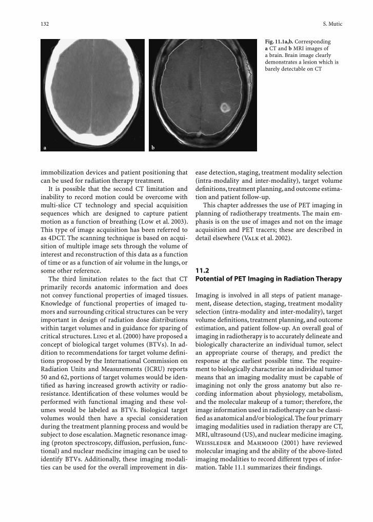
132 S. Mutic

immobilization devices and patient positioning that can be used for radiation therapy treatment.

It is possible that the second CT limitation and inability to record motion could be overcome with multi-slice CT technology and special acquisition sequences which are designed to capture patient motion as a function of breathing (Low et al. 2003). This type of image acquisition has been referred to as 4DCT. The scanning technique is based on acqui-sition of multiple image sets through the volume of interest and reconstruction of this data as a function of time or as a function of air volume in the lungs, or some other reference.

The third limitation relates to the fact that CT primarily records anatomic information and does not convey functional properties of imaged tissues. Knowledge of functional properties of imaged tu-mors and surrounding critical structures can be very important in design of radiation dose distributions within target volumes and in guidance for sparing of critical structures. Ling et al. (2000) have proposed a concept of biological target volumes (BTVs). In ad-dition to recommendations for target volume defi ni-tions proposed by the International Commission on Radiation Units and Measurements (ICRU) reports 50 and 62, portions of target volumes would be iden-tifi ed as having increased growth activity or radio-resistance. Identifi cation of these volumes would be performed with functional imaging and these vol-umes would be labeled as BTVs. Biological target volumes would then have a special consideration during the treatment planning process and would be subject to dose escalation. Magnetic resonance imag-ing (proton spectroscopy, diffusion, perfusion, func-tional) and nuclear medicine imaging can be used to identify BTVs. Additionally, these imaging modali-ties can be used for the overall improvement in dis-

ease detection, staging, treatment modality selection (intra-modality and inter-modality), target volume defi nitions, treatment planning, and outcome estima-tion and patient follow-up.

This chapter addresses the use of PET imaging in planning of radiotherapy treatments. The main em-phasis is on the use of images and not on the image acquisition and PET tracers; these are described in detail elsewhere (Valk et al. 2002).

11.2 Potential of PET Imaging in Radiation Therapy

Imaging is involved in all steps of patient manage-ment, disease detection, staging, treatment modality selection (intra-modality and inter-modality), target volume defi nitions, treatment planning, and outcome estimation, and patient follow-up. An overall goal of imaging in radiotherapy is to accurately delineate and biologically characterize an individual tumor, select an appropriate course of therapy, and predict the response at the earliest possible time. The require-ment to biologically characterize an individual tumor means that an imaging modality must be capable of imagining not only the gross anatomy but also re-cording information about physiology, metabolism, and the molecular makeup of a tumor; therefore, the image information used in radiotherapy can be classi-fi ed as anatomical and/or biological. The four primary imaging modalities used in radiation therapy are CT, MRI, ultrasound (US), and nuclear medicine imaging. Weissleder and Mahmood (2001) have reviewed molecular imaging and the ability of the above-listed imaging modalities to record different types of infor-mation. Table 11.1 summarizes their fi ndings.

Fig. 11.1a,b. Corresponding a CT and b MRI images of a brain. Brain image clearly demonstrates a lesion which is barely detectable on CT

ba

PET and PET/CT for Radiotherapy Planning 133

Table 11.1. Information content of current imaging modalities in radiotherapy

Anatomy Physiology Metabolism Molecular

CT

US

MRI

Nuclear

The PET superior biological tumor information can be used for disease detection, staging, therapy selection, target design, outcome prognosis, and fol-low-up.

Detection. Imaging of disease with CT or MRI (non-functional) is based on anatomical or physio-logical changes that are a late manifestation of molec-ular changes that underlie the disease. By detecting changes in the molecular and biochemical process, biological imaging can demonstrate disease before it becomes anatomically detectable with CT or MRI. Changes in tumor detection capabilities can lead to modifi cation in radiation therapy target volumes and dose prescriptions.

Staging. PET has improved patient staging in sev-eral treatment sites (Dizendorf et al. 2003). Better knowledge of the true extent of the patient’s disease can signifi cantly alter patient management. For some patients who would otherwise undergo curative ra-diotherapy PET may demonstrate distal disease or al-ter the extent of local disease and indicate that a pal-liative course of therapy is more appropriate. These patients would not only be spared the side effects of futile curative treatment, but the overall health care costs could also be lowered due to PET fi ndings.

For example, MacManus et al. (2001) prospec-tively studied 153 patients with unresectable non-small-cell lung carcinoma (NSCLC) who were can-didates for radical radiotherapy after conventional staging and who have undergone a PET scan. These patients were staged based on pre-PET and post-PET imaging. The authors used survival analysis to vali-date pre-PET and post-PET staging. Forty-six patients (30%) received palliative treatment because of PET-detected distant metastasis or extensive locoregional disease. Five patients were down-staged due to PET fi ndings and underwent radical surgery. The remain-ing 102 patients underwent radical radiotherapy with or without concurrent chemotherapy. For 22 of these 102 patients, there was a signifi cant increase in tar-get volume due to PET imaging and 16 patients had a signifi cant reduction in target volumes due to use

of PET images in treatment planning. Additionally, for the 102 radically treated patients, post-PET stage, but not pre-PET stage, correlated strongly with the survival. As pointed out by the authors, the entire radical radiotherapy literature for NSCLC may have to be reevaluated due to inclusion of a large portion of patients with an incurable disease in clinical tri-als. It is possible that many trials failed to show any signifi cant benefi t of proposed treatment strategies due to inclusion of these patients. Had the PET been available, these studies would have evaluated a more appropriate cohort of patients.

In addition to more accurate staging, PET may also be able to provide information about individual tumor biology (phenotype). This would allow fur-ther stratifi cation of patients within the same clinical stage. So rather than basing therapy selection for an individual patient on the stage alone, which is statis-tically appropriate for a large group of patients, bio-logical properties of an individual tumor can then be used for therapy selection. The tumor phenotype information may affect inter-modality and intra-mo-dality patient management depending on suspected radiation or chemotherapy sensitivity of an individ-ual tumor. If we know more about biological proper-ties of an individual tumor, it may be possible to in-corporate biological response models in the therapy selection process to maximize the therapeutic ratio.

Target defi nition and altered dose distributions. As stated previously, the true extent of the disease may extend beyond anatomically defi ned volumes and PET has already been shown to be valuable for defi ning the extent of target volumes. Furthermore, PET can be used to differentiate areas of biological importance within the boundaries of target volumes. It is possible that the concept of BTVs can be imple-mented with PET and that doses can be escalated to these BTVs if deemed necessary.

For example, Chao et al. (2001) have shown how PET imaging based hypoxia measurement technique with Cu(II)-diacetyl-bis(N4-methylthiosemicarba-zone) (Cu-ATSM) tracer can be used to identify a BTV

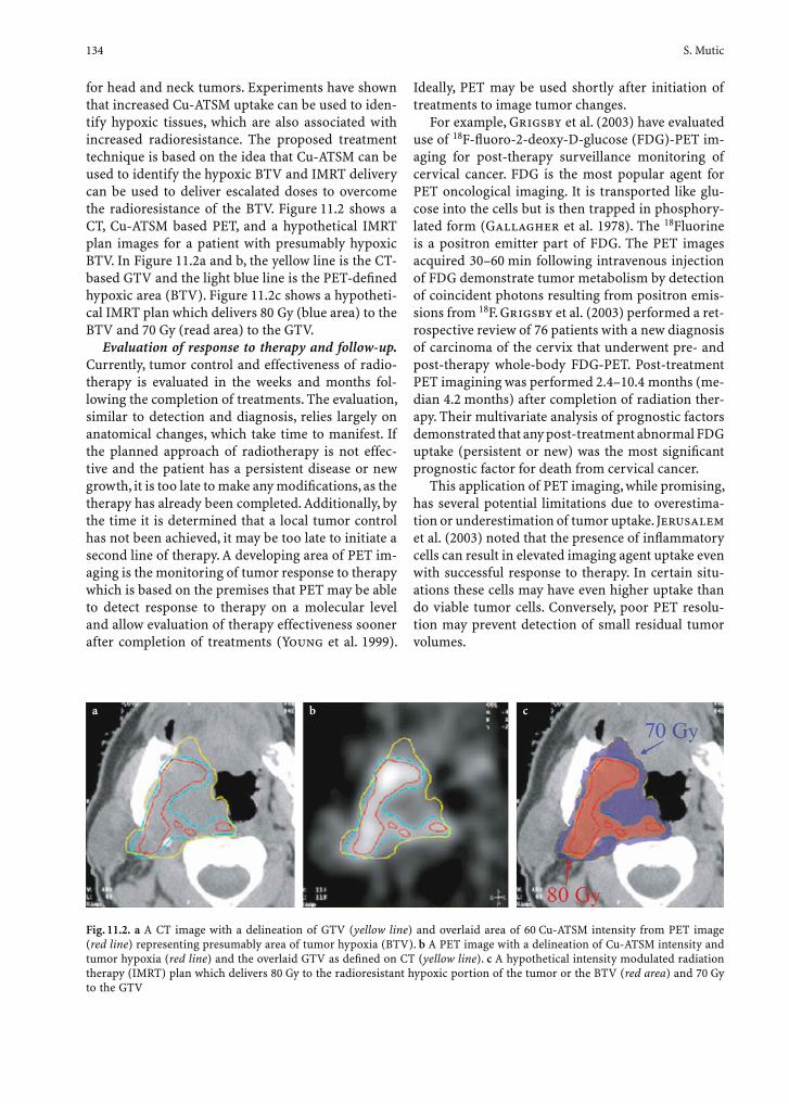
134 S. Mutic

for head and neck tumors. Experiments have shown that increased Cu-ATSM uptake can be used to iden-tify hypoxic tissues, which are also associated with increased radioresistance. The proposed treatment technique is based on the idea that Cu-ATSM can be used to identify the hypoxic BTV and IMRT delivery can be used to deliver escalated doses to overcome the radioresistance of the BTV. Figure 11.2 shows a CT, Cu-ATSM based PET, and a hypothetical IMRT plan images for a patient with presumably hypoxic BTV. In Figure 11.2a and b, the yellow line is the CT-based GTV and the light blue line is the PET-defi ned hypoxic area (BTV). Figure 11.2c shows a hypotheti-cal IMRT plan which delivers 80 Gy (blue area) to the BTV and 70 Gy (read area) to the GTV.

Evaluation of response to therapy and follow-up. Currently, tumor control and effectiveness of radio-therapy is evaluated in the weeks and months fol-lowing the completion of treatments. The evaluation, similar to detection and diagnosis, relies largely on anatomical changes, which take time to manifest. If the planned approach of radiotherapy is not effec-tive and the patient has a persistent disease or new growth, it is too late to make any modifi cations, as the therapy has already been completed. Additionally, by the time it is determined that a local tumor control has not been achieved, it may be too late to initiate a second line of therapy. A developing area of PET im-aging is the monitoring of tumor response to therapy which is based on the premises that PET may be able to detect response to therapy on a molecular level and allow evaluation of therapy effectiveness sooner after completion of treatments (Young et al. 1999).

Ideally, PET may be used shortly after initiation of treatments to image tumor changes.

For example, Grigsby et al. (2003) have evaluated use of 18F-fl uoro-2-deoxy-D-glucose (FDG)-PET im-aging for post-therapy surveillance monitoring of cervical cancer. FDG is the most popular agent for PET oncological imaging. It is transported like glu-cose into the cells but is then trapped in phosphory-lated form (Gallagher et al. 1978). The 18Fluorine is a positron emitter part of FDG. The PET images acquired 30–60 min following intravenous injection of FDG demonstrate tumor metabolism by detection of coincident photons resulting from positron emis-sions from 18F. Grigsby et al. (2003) performed a ret-rospective review of 76 patients with a new diagnosis of carcinoma of the cervix that underwent pre- and post-therapy whole-body FDG-PET. Post-treatment PET imagining was performed 2.4–10.4 months (me-dian 4.2 months) after completion of radiation ther-apy. Their multivariate analysis of prognostic factors demonstrated that any post-treatment abnormal FDG uptake (persistent or new) was the most signifi cant prognostic factor for death from cervical cancer.

This application of PET imaging, while promising, has several potential limitations due to overestima-tion or underestimation of tumor uptake. Jerusalem et al. (2003) noted that the presence of infl ammatory cells can result in elevated imaging agent uptake even with successful response to therapy. In certain situ-ations these cells may have even higher uptake than do viable tumor cells. Conversely, poor PET resolu-tion may prevent detection of small residual tumor volumes.

Fig. 11.2. a A CT image with a delineation of GTV (yellow line) and overlaid area of 60 Cu-ATSM intensity from PET image (red line) representing presumably area of tumor hypoxia (BTV). b A PET image with a delineation of Cu-ATSM intensity and tumor hypoxia (red line) and the overlaid GTV as defi ned on CT (yellow line). c A hypothetical intensity modulated radiation therapy (IMRT) plan which delivers 80 Gy to the radioresistant hypoxic portion of the tumor or the BTV (red area) and 70 Gy to the GTV

ba c

PET and PET/CT for Radiotherapy Planning 135

11.3 Technology Overview

Imaging for radiotherapy treatment planning and medical imaging in general are continually evolv-ing. All three major imaging modalities (CT, MRI, and PET) have undergone signifi cant changes during the past decade. One of the major changes in radio-therapy imaging is the approach of imaging equip-ment manufacturers towards radiation oncology and its unique imaging needs. Radiotherapy imaging has special needs with respect to scanner geometry, pa-tient positioning, and target delineation. These needs are often not a signifi cant concern in diagnostic ra-diology. The scanners used in radiotherapy should have fl at tabletops, larger openings to accommodate immobilization devices and patients in conventional treatment positions, and software tools which can improve patient positioning and target delineation (Mutic et al. 2003a). Until the late 1990s, imaging equipment was designed and manufactured, almost exclusively, with diagnostic radiology needs in mind, and these devices would then have to be modifi ed for therapy scanning and frequently there were sig-nifi cant limitations. In the past few years there have been a number of scanners introduced on the market with features designed specifi cally for radiotherapy. Radiotherapy needs have begun to drive product de-velopment. This change in manufacturer approach towards radiotherapy has resulted in a variety of imaging options available to radiation oncology de-partments, and it has improved our ability to image patients for treatment planning purposes.

With respect to the use of PET in treatment plan-ning, three scanner types need to be considered: stand-alone CT; stand-alone PET; and combined PET/CT scanners. A variety of these devices are of-fered from several manufacturers and their imple-mentation differs greatly. The major differences are with respect to scanner geometry (size of the bore opening), number and/or length of the images that can be acquired simultaneously, detector type and design, image reconstruction capabilities, and tools designed for radiotherapy purposes. Physics and de-tailed instrumentation analysis of these devices is beyond the scope of this text and more comprehen-sive reviews have been published by Bailey (2003), Bailey et al. (2003), Defrise et al. (2003), and Meikle and Badawi (2003). The technical overview of these devices presented here concentrates on features that uniquely affect scanning for radiotherapy treatment planning and our ability to accurately defi ne location of tumor volumes (spatially and temporally).

11.3.1 CT

The two most signifi cant changes in CT technology, for radiation therapy scanning purposes, in recent years have been the introduction of a larger gantry bore opening (large-bore CT; Garcia-Ramirez et al. 2002) and multi-slice image acquisition (multi-slice CT; Klingenbeck et al. 1999).

Large-Bore CT. Large-bore CT scanners were spe-cifi cally designed with radiation therapy needs in mind. One of the requirements in treatment of sev-eral cancer sites (breast, lung, vulva, etc.) is for ex-tremities to be positioned away from the torso. When acquiring a CT scan with a patient in such treatment position, extremities often cannot fi t through a con-ventional 70-cm diameter scanner bore opening. In such situations, patient positioning needs to be modifi ed in order to acquire the scan. This can re-sult in less optimal treatment position (patient may be less comfortable and therefore the daily setup re-producibility may be compromised). Large immobi-lization devices (slant board, body moulds) may also be diffi cult to fi t through a conventional diameter scanner. With these obstacles in mind, an 85-cm di-ameter scanner was introduced in 2000 and virtually eliminated the aforementioned problems. Since then, other manufacturers have introduced 80- and 82-cm-diameter scanners.

The 85-cm scanner also has a 60-cm-scan fi eld of view (SFOV), compared with 48-cm SFOV on most conventional scanners. For treatment planning pur-poses it is necessary to have the full extent of the patient’s skin on the CT image. Lateral patient sepa-ration can often be larger than 48 cm and the skin is then not visible on a 48-cm SFOV scan. Increased SFOV solves this problem and several CT scanners now have images which extend beyond 48 cm.

Multi-slice CT. In 1992 Elscint (Haifa, Israel) intro-duced a scanner which had a dual row of detectors and could acquire two images (slices) simultaneously. Since then, multi-slice CT has gained widespread ac-ceptance, and scanners which can acquire 4, 8, 10, 16, 32, 40, 64, etc. are now available. The primary advan-tage of multi-slice scanners is the ability to acquire image studies faster than single-slice scanners. For example, a 4-slice helical CT can provide equivalent image quality at two to three times the volume cover-age speed of a single-slice helical CT. Similarly, scan-ners with a greater number of slices are even faster.

One of the obstacles for radiation therapy scan-ning with single slice scanners is the limited tube-heat loading capability. Often, fewer images are taken,

136 S. Mutic

slice thickness is increased, mAs is decreased, or scan pitch is increased to reduce the amount of heat pro-duced during the scan and to allow for the entire scan to be acquired in a single acquisition. Due to the lon-ger length of imaged volume per tube rotation, (mul-tiple slices acquired simultaneously), the tube heat loading for a particular patient volume is lower for multi-slice than for single-slice scanners, and multi-slice scanners are generally not associated with tube head-loading concerns. Faster acquisition times and decreased tube loading of multi-slice scanners (which will allow longer volumes to be scanned in a single ac-quisition) can potentially provide an advantage over single-slice systems for treatment planning purposes. Multi-slice technology can be especially benefi cial for imaging of the thorax where breathing artifacts can be minimized. This technology can also be valuable for simulation of respiratory-gated treatments.

Multi-slice scanners are also capable of acquir-ing thinner slices which can result in better-quality DRRs and more accurate target delineation (better spatial resolution). Studies with thinner slices result in an increased number of images to process. Target volumes and critical structures have to be delineated on an increased number of images and treatment-planning systems have to handle larger amounts of data. Currently, this can result in increased time and labor required for treatment planning. Software ven-dors are creating tools which will allow easier ma-nipulation of larger study sets but which will likely take several years to implement. In the meantime, the number of CT images that are acquired for a treat-ment plan needs to be balanced between resolution requirements and the ability to process larger num-bers of images.

11.3.2 PET

The PET images for radiotherapy planning can come from a stand-alone PET scanner or a combined PET/CT unit. Combined PET/CT scanners offer several advantages for radiotherapy imaging and are gen-erally preferred over stand-alone units; however, stand-alone scanners have been successfully used for radiotherapy imaging, and due to a large installed base will continue to be used for this purpose in the foreseeable future.

One of the main differences between a stand-alone PET scanner and a combined PET/CT unit is the method of gathering data to generate PET attenua-tion correction factors (ACFs). As described in detail

by Meikle and Badawi (2003), PET imaging relies on the simultaneous detection (a coincident event) of both photons which were created from annihilation of a positron. Coincident detection will not occur if either of the photons is absorbed or scattered from the fi eld of view. The probability of absorption or scat-tering depends on the total path length for the two photons. The attenuation probability is the same for all source points that lie on a line which links two de-tectors (line of response), since the total path length to these detectors is the same for all photon pairs cre-ated on that line. The ACFs for each line of response can be determined from transmission measurements for an external (transmission) source. Transmission measurements typically rely on long-lived, external, positron sources. The source-detector confi guration for transmission measurements has evolved over time and varies between different scanner designs. For reasons described elsewhere (Meikle and Badawi 2003), transmission measurements constitute a major portion (up to 30 min for whole-body PET studies) of the total time required for a PET scan and are also a major source of noise in reconstructed PET images. As described in the next section, the use of CT for at-tenuation correction in PET/CT scanners can improve both of these problems. The benefi t of transmission (attenuation correction) images from a stand-alone PET scanner for radiotherapy treatment planning, as described later in this chapter, is that they can be used to determine registration transformations for regis-tration of emission images with a CT scan.

One of the major limitations of stand-alone PET scanners is a relatively small gantry bore opening, typically 55–60 cm. These scanners were designed to optimize image quality and not necessarily to accom-modate radiotherapy patients in treatment positions with immobilization devices. This design feature of stand-alone PET scanners can severely limit the size of immobilization devices and patient position that is used for treatment.

Stand-alone PET scanners were also intended to have curved tabletops. For radiotherapy scanning, a PET scanner needs to have a fl at tabletop. To correct this, typically a fl at tabletop is acquired from a third-party vendor and installed over the curved top. The fl at tabletop can be an overlay type, where a fl at board rests on the tips of the curved couch (Fig. 11.3a) or an insert type which is fl at on one side and curved on the other side to match the curvature of the factory installed tabletop (Figs. 11.3b, c). An overlay type, like in Fig. 11.3a, has same dimensions as the treatment table on a linear accelerator and is preferred for im-aging patients for radiotherapy planning; however,

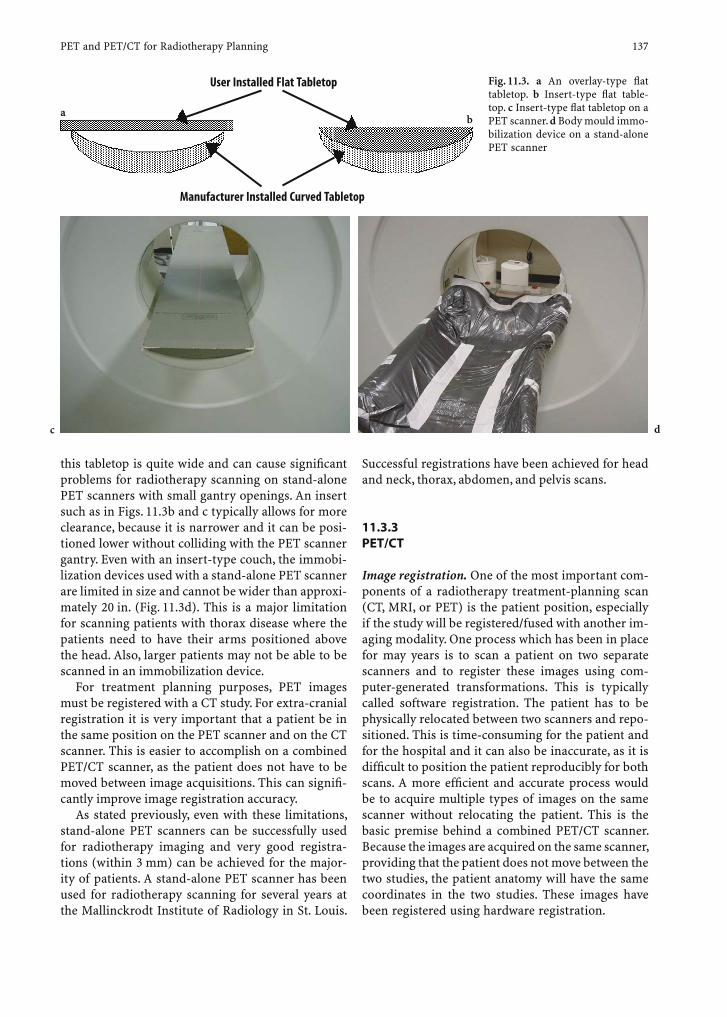
PET and PET/CT for Radiotherapy Planning 137

this tabletop is quite wide and can cause signifi cant problems for radiotherapy scanning on stand-alone PET scanners with small gantry openings. An insert such as in Figs. 11.3b and c typically allows for more clearance, because it is narrower and it can be posi-tioned lower without colliding with the PET scanner gantry. Even with an insert-type couch, the immobi-lization devices used with a stand-alone PET scanner are limited in size and cannot be wider than approxi-mately 20 in. (Fig. 11.3d). This is a major limitation for scanning patients with thorax disease where the patients need to have their arms positioned above the head. Also, larger patients may not be able to be scanned in an immobilization device.

For treatment planning purposes, PET images must be registered with a CT study. For extra-cranial registration it is very important that a patient be in the same position on the PET scanner and on the CT scanner. This is easier to accomplish on a combined PET/CT scanner, as the patient does not have to be moved between image acquisitions. This can signifi -cantly improve image registration accuracy.

As stated previously, even with these limitations, stand-alone PET scanners can be successfully used for radiotherapy imaging and very good registra-tions (within 3 mm) can be achieved for the major-ity of patients. A stand-alone PET scanner has been used for radiotherapy scanning for several years at the Mallinckrodt Institute of Radiology in St. Louis.

Successful registrations have been achieved for head and neck, thorax, abdomen, and pelvis scans.

11.3.3 PET/CT

Image registration. One of the most important com-ponents of a radiotherapy treatment-planning scan (CT, MRI, or PET) is the patient position, especially if the study will be registered/fused with another im-aging modality. One process which has been in place for may years is to scan a patient on two separate scanners and to register these images using com-puter-generated transformations. This is typically called software registration. The patient has to be physically relocated between two scanners and repo-sitioned. This is time-consuming for the patient and for the hospital and it can also be inaccurate, as it is diffi cult to position the patient reproducibly for both scans. A more effi cient and accurate process would be to acquire multiple types of images on the same scanner without relocating the patient. This is the basic premise behind a combined PET/CT scanner. Because the images are acquired on the same scanner, providing that the patient does not move between the two studies, the patient anatomy will have the same coordinates in the two studies. These images have been registered using hardware registration.

Fig. 11.3. a An overlay-type fl at tabletop. b Insert-type fl at table-top. c Insert-type fl at tabletop on a PET scanner. d Body mould immo-bilization device on a stand-alone PET scanner

User Installed Flat Tabletop

Manufacturer Installed Curved Tabletop

ba

c d

138 S. Mutic

Scan time. One additional benefi t of the combined PET/CT unit is that CT images are used for attenua-tion correction of the PET emission data, obviating the need for a time-consuming PET transmission scan. The use of CT images to generate PET ACFs reduces the scan time by up to 40% and also pro-vides essentially noiseless ACFs compared with those from standard PET transmission measurements (Townsend et al. 2004). Shorter scan times can ben-efi t radiotherapy patients who are scanned in treat-ment position which often can be uncomfortable and diffi cult to tolerate for prolonged periods of time.

Attenuation correction factors. One of the con-cerns with ACFs generated from CT images is mis-match or misalignment between CT and PET images. The PET images are acquired during many cycles of free breathing and CT images are acquired as a snapshot in time at full inspiration, partial inspira-tion, or some form of shallow breathing. The breath-ing motion will cause mismatch in anatomy between PET and CT images in the base of lung and through the diaphragm region. This mismatch can result in artifacts in these areas which may infl uence diagno-sis and radiotherapy target defi nition in this region. There are various gating methods that can be used during image acquisition to minimize the motion component and essentially acquire true, motionless, images of patient anatomy. Gated or 4DCT (with time being the fourth dimension) can be used to generate more reliable ACFs and also for radiotherapy treat-ment planning where gated delivery methods are be-ing used.

Contrast-enhanced CT images can cause inaccu-rate ACFs due to artifi cially increased attenuation through anatomy which contains contrast material. The most obvious way to avoid this problem is to ac-quire a routine CT with contrast and another non-contrast CT. There is also an option to use software tools to correct for these artifacts. As discussed later, for radiotherapy scanning, it is preferred to acquire two separate scans. The attenuation correction CT can be a whole-body, low-dose scan with greater slice thickness, if desired. The second CT would be a treatment-planning scan with thin slices for bet-ter resolution and DRR quality. This scan is acquired only through the volume of interest thus limiting the number of images and memory requirements to manipulate these images in the treatment-planning computer. This second scan can then be contrast en-hanced, if desired.

The fi rst combined PET/CT prototype was intro-duced in 1998 at the University of Pittsburgh (Beyer et al. 2000). The PET detectors were mounted on the

same rotating assembly as the CT, 60 cm away from the CT imaging plane. Since then, several models have been introduced by major manufacturers of medi-cal imaging devices. The key description of PET/CT scanners is that PET and CT scanners are combined in the same housing (Fig. 11.4), meaning that there are two gantries (PET and CT) combined in one housing sharing a common couch. Image reconstruction and scanner operation is increasingly performed from one control console.

Fig. 11.4. A combined PET/CT scanner

Combined PET/CT scanner design varies among different vendors with respect to PET detectors, im-age quality and resolution, speed, and imaging fi eld of view; number of slices for the CT part, scanner couch design, gantry bore opening, and other con-siderations. All of the commercially available scan-ners have a 70-cm gantry opening for the CT portion. The PET gantry opening ranges in diameter from 60 to 70 cm, meaning that some of the commercial scanners have a non-uniform gantry opening as the patient travels from the CT portion of the scanner to the PET side. More importantly, the scanners with the smaller gantry opening on the PET side will pose the same diffi culties for radiotherapy scanning as stand-alone PET scanners. Again, the size of patient immobilization devices and patient scan/treatment position will have to be adapted to the size of the gantry opening.

11.4 Treatment Planning with PET

As previously described, PET images can be used at multiple stages of radiation therapy patient manage-ment (detection, staging, treatment planning, treat-

PET and PET/CT for Radiotherapy Planning 139

ment effi cacy evaluation, and follow-up). For treat-ment-planning purposes, PET is used to delineate target volumes. Role of PET in oncologic imaging for purposes of diagnosis, staging, and patient man-agement is well defi ned and understood. The PET is routinely used for the imaging of many disease sites and its importance has been established and documented through hundreds of clinical trials and studies. The value of PET for identifi cation and de-lineation of target volumes in radiotherapy treatment planning is yet to be adequately explored and appre-ciated. Reports of PET use for radiotherapy treatment planning in literature have been largely limited to relatively small numbers of patients with brain tu-mors, head and neck tumors, NSCLC, or gynecologic tumors. There are several reasons for a relatively lim-ited use of PET imaging for target volume delineation in radiotherapy. Until recently, many treatment-plan-ning systems were not able to accept PET images. The PET scanning for radiotherapy treatment planning with stand-alone PET scanners can appear techni-cally daunting to implement. The approval and reim-bursement criteria for a separate treatment-planning PET scan, after a diagnostic scan has already been acquired, has not been adequately defi ned. Edges of tumor volumes on PET images are smeared and their contouring can be quite subjective (Mah et al. 2002; Erdi et al. 1997), and robust user-independent meth-ods are still under development. Finally, it is unclear whether the use of PET images for target delineation will improve outcomes and/or reduce treatment re-lated complications.

The PET scanning for radiotherapy treatment planning is similar to CT scanning in radiation on-cology. The process consists of patient immobiliza-tion, scan, image transfer, registration of PET and CT images, structure delineation, and dose calculation. The following sections describe how this process was implemented at the Mallinckrodt Institute of Radiology. This implementation can vary among in-stitutions depending on the available equipment and resources, and desired clinical end points.

11.4.1 Patient Positioning and Immobilization

A PET scanner needs several modifi cations for ra-diotherapy scanning. As shown in Fig. 11.3, the PET scanner requires a fl at couch top. Flat tabletops are often provided by the manufacturers with the newer PET/CT scanner. Older stand-alone scanners typi-cally do not have fl at tabletops available from the

manufacturers. Third-party vendors also do not supply fl at tabletops specifi cally manufactured for PET scanner. Flat tabletops designed for CT scan-ners should work well on PET scanners. Figure 11.3c shows such a setup.

Whether using a stand-alone PET scanner or a PET/CT unit, the scanner room should be equipped with external patient alignment lasers. The external lasers should consist of an overhead laser and two lat-eral wall lasers. In CT-simulator rooms, the overhead laser is almost always movable in the lateral direc-tion. The latter wall lasers can be fi xed or movable. For the use of stand-alone PET scanners, the patient is typically fi rst scanned in a CT simulator where an immobilization device is manufactured and the pa-tient is marked. In this situation, the patient arrives to the PET scanner marked and the alignment lasers are used only for patient positioning. The overhead and wall lasers on a stand-alone PET scanner do not need to be mobile. As the overhead laser is not movable, setup marks should be placed on the patient with the CT simulator overhead laser at center position. These marks do not have to correspond to the iso-center point and can be removed after the PET scan. For PET/CT installation, where the treatment-plan-ning CT may also be acquired, the room should be equipped with external lasers where at minimum the overhead laser is movable. These lasers should be po-sitioned and aligned as recommended by the AAPM Task Group 66 report (Mutic et al. 2003a).

Patient immobilization devices should be small enough to fi t through possibly smaller PET-scanner openings. Due to relatively expensive and demanding time on a PET scanner, immobilization devices are typically premanufactured on a conventional simula-tor or CT simulator. It is important to predefi ne the maximum size of immobilization devices that can be used in a PET scanner to ensure that the patient and the immobilization device will fi t through a PET scanner. Generally, if the immobilization device con-struction and materials are suitable for CT imaging, they should be appropriate for PET as well.

11.4.2 Scan

CT. The CT scan parameters for PET-based treat-ment planning are the same as for routine treatment-planning CT studies. If the images are acquired on a stand-alone CT scanner, routine oncology protocols should be used. If the patient is scanned on a PET/CT scanner, two CT scans should be acquired. The

140 S. Mutic

fi rst CT scan is the attenuation correction CT which will span long volumes and it is generally acquired with thicker image slices and spacing. This scan is not adequate for most radiotherapy treatment plan-ning. The second CT is a treatment-planning CT with thinner slices (3 mm or thinner), possibly with scan parameters designed to optimize image content re-quired for target delineation. This scan may also be acquired with contrast. The treatment planning CT should span shorter volumes, through the region of interest plus a 5- to 10-cm margin.

PET. The PET scanning for radiotherapy treat-ment planning is generally the same as diagnostic scanning. The PET treatment-planning studies can be narrowed down to include only the region sur-rounding the tumor and do not have to be as long as diagnostic scans. This is not a major time- and cost-savings concern; it actually may be more benefi cial to acquire another full volume scan to possibly detect any new distant metastasis. Just as diagnostic CT re-quirements are not the same as radiotherapy image-acquisition needs, so there are differences in acquisi-tion needs between diagnostic and radiotherapy PET scans. Development of radiotherapy-specifi c PET-ac-quisition protocols is an area which should be very active during the next several years.

11.4.3 Image Transfer and Registration

The CT study set is almost always the primary data on which the isodoses are computed and displayed due to its high spatial resolution and fi delity. The exceptions are some stereotactic radiosurgery and brachytherapy applications where MRI or US, respec-tively, are used as the primary studies. When properly calibrated and free of image artifacts, CT images can provide electron-density information for heterogene-ity-based dose calculations. As previously described, CT images do have shortcomings and other imaging modalities can offer unique information about tu-mor volumes. If other imaging modalities are used in the treatment-planning process, they are typically considered secondary data sets and must be spatially registered to the CT study to accurately aid in tumor-volume delineation.

Registration of multimodality images is a sev-eral-step process requiring multi-function software capable of image-set transfer, storage, coordinate transformation, and voxel interpolation. These fea-tures enable image study registration (transforming images to a common reference frame and resampling

to a common pixel grid) and fusion (the display of a combination of pixel intensities from registered im-age studies). Registered and “fused” image studies can then be used for radiotherapy treatment planning.

Images and other treatment-planning data are transferred between modern systems using Digital Image Communications in Medicine (DICOM) stan-dard (NEMA 1998). DICOM is a standard for repre-senting and exchanging medical imaging data. Many of the older PET scanners do not have DIOCM ex-port capabilities and some other software is needed to enable image transfer between these scanners and radiotherapy treatment planning. This is often one of greater obstacles in using older stand-alone PET scanners for radiotherapy imaging.

If a PET/CT scanner is used to acquire treat-ment-planning images, these images are acquired on a common platform and two data sets are spatially registered by hardware. At the time of publication of this book, registration information is not a part of DICOM object set. It is because of this that, when PET and CT studies are transferred from a PET/CT scan-ner to a treatment-planning system, these images will not be considered registered by the treatment-plan-ning computer and some form of image registration will have to be performed. As the two data sets should already be on a common matrix and have the same spatial position and orientation, data registration in most treatment-planning systems can be achieved without any image manipulation. If either of the data sets is resampled or manipulated during the import into the treatment planning system, then image com-monality between two data sets may not have been preserved and data sets will have to be realigned to be registered.

The PET and CT images that are acquired on separate scanners have to be registered in the treat-ment-planning system. There are several methods for image registration. Surface-based registration requires contouring of the same structure (internal or external) on the two data sets and the studies are then registered by aligning the contours. Edges of organs on PET images are poorly defi ned and sur-face-based registration typically cannot be used for image registration. Image-based registration involves displaying CT data set in background, in gray scale, and superimposing the PET image in color wash or in gray scale on top of the CT study. The two stud-ies are typically simultaneously viewed in transverse, sagittal, and coronal orientation. The studies are then registered by manipulating PET images in three displayed planes. This registration method works reasonably well, especially if FDG is used as a PET

PET and PET/CT for Radiotherapy Planning 141

imaging agent. Image-based registration of PET im-ages acquired with some other imaging agents, such as 60Cu-ATSM, may be very diffi cult to perform as the image content in PET and CT images can be substan-tially different. For such studies, transmission PET images can be fi rst registered with CT images using image-based registration. Transmission PET im-ages can reveal many anatomical features similar to those of X-ray CT. The image transformations from this registration can then be used to register emis-sion scans to the CT study. This is a relatively slow process as two PET scans are required. Point-based registration is based on identifying a set of at least three corresponding points in both data sets and performing image transforms to align these points. Point-based registration works well for CT and MRI as there are numerous anatomical points which are identifi able on both studies. Point-based registration with PET, using anatomic points, is virtually impos-sible due to poor image resolution; however, point-based registration of PET images with fi ducial mark-ers is extremely useful. Figure 11.5 shows PET and CT images registered using fi ducial markers. Markers used in this fi gure were made with 0.5-cm diameter, 3.5-cm long, 0.25-ml plastic, disposable microcentri-fuge tubes (VWRbrand Disposable Microcentrifuge

Tubes, VWR Scientifi c Products, West Chester, Pa.) commonly found in chemistry and biology laborato-ries (Mutic et al. 2001). One end of the ampoules is conical and the other end can be opened and closed with a small cap (Fig. 11.6a). For CT scans, two small pieces of aluminum wire are placed at the pointed end of the ampoules and secured in place with dental wax. For PET scans, a small drop of 18F-FDG is placed at the pointed end of the fi ducial marker. The drop is held in place by liquid surface tension. The surface tension is strong enough that the fi ducial marker can be handled without worry that the drop may be dis-placed. Also for PET scans, the radioactive material is safely contained in the plastic ampoules.

As the fi ducial markers are unique for each imag-ing modality, there has to be a mechanism to repro-ducibly replace them between the scans. For head and neck scans, the markers are rigidly and reproducibly attached to the patient thermoplastic immobilization mask using a small piece of thermoplastic material. For these scans it is assumed that the patient position between two scans is closely (within 3 mm) repro-duced by the thermoplastic mask. For body scans, it is more diffi cult to reproducibly attach markers to the patient. The main diffi culty is that markers move with patient skin. To minimize the uncertainty due to skin

Fig. 11.5. Point-based registration using fi ducial markers. Images on the left are axial and coronal PET planes and images on the right are the corresponding CT planes. Arrows are pointing to the same fi -ducial marker on all four images

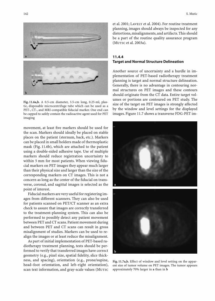
142 S. Mutic

movement, at least fi ve markers should be used for the scan. Markers should ideally be placed on stable places on the patient (sternum, back, etc.). Markers can be placed in small holders made of thermoplastic mask (Fig. 11.6b), which are attached to the patient using a double-sided adhesive tape. Use of multiple markers should reduce registration uncertainty to within 5 mm for most patients. When viewing fi du-cial markers on PET images they appear much larger than their physical size and larger than the size of the corresponding markers on CT images. This is not a concern as long as the center of the fi ducial on trans-verse, coronal, and sagittal images is selected as the point of interest.

Fiducial markers are very useful for registering im-ages from different scanners. They can also be used for patients scanned on PET/CT scanner as an extra check to assure that images are correctly transferred to the treatment-planning system. This can also be performed to possibly detect any patient movement between PET and CT scans. Patient movement during and between PET and CT scans can result in gross misalignment of studies. Markers can be used to re-align the images or at least reduce the misalignment.

As part of initial implementation of PET-based ra-diotherapy treatment planning, tests should be per-formed to verify that transferred images have correct geometry (e.g., pixel size, spatial fi delity, slice thick-ness, and spacing), orientation (e.g., prone/supine, head–foot orientation, and left–right orientation), scan text information, and gray-scale values (Mutic

et al. 2001; Lavely et al. 2004). For routine treatment planning, images should always be inspected for any distortions, misalignments, and artifacts. This should be a part of the routine quality assurance program (Mutic et al. 2003a).

11.4.4 Target and Normal Structure Delineation

Another source of uncertainty and a hurdle in im-plementation of PET-based radiotherapy treatment planning is target and normal structure delineation. Generally, there is no advantage in contouring nor-mal structures on PET images and these contours should originate from the CT data. Entire target vol-umes or portions are contoured on PET study. The size of the target on PET images is strongly affected by the window and level settings for the displayed images. Figure 11.7 shows a transverse FDG-PET im-

b

a

Fig. 11.6a,b. A 0.5-cm diameter, 3.5-cm long, 0.25-ml, plas-tic, disposable microcentrifuge tube which can be used as a PET-, CT-, and MRI-compatible fi ducial marker. One end can be capped to safely contain the radioactive agent used for PET imaging

Fig. 11.7a,b. Effect of window and level setting on the appar-ent size of tumor volume on PET images. The tumor appears approximately 70% larger in a than in b

b

a

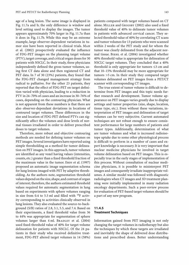
PET and PET/CT for Radiotherapy Planning 143

age of a lung lesion. The same image is displayed in Fig. 11.7a and b; the only difference is window and level setting used to display the images. The tumor appears approximately 70% larger in Fig. 11.7a than it does in Fig. 11.7b. While this may be an extreme example, large observer-dependent variations in tu-mor size have been reported in clinical trials. Mah et al. (2002) prospectively evaluated the infl uence of FDG-PET images on the planning target volume (PTV), target coverage, and critical organ doses for 30 patients with NSCLC. In their study, three physicians independently defi ned the gross tumor volumes, us-ing fi rst CT data alone and then registered CT and PET data. In 7 of 30 (23%) patients, they found that the FDG-PET changed management strategy from radical to palliative. For the other 23 patients, they reported that the effect of FDG-PET on target defi ni-tion varied with physician, leading to a reduction in PTV in 24–70% of cases and an increase in 30–76% of cases, depending on the contouring physician. What is not apparent from these numbers is that there are also observer-dependant deviations in locations of contoured target volumes. These differences in the size and location of FDG-PET defi ned PTVs can sig-nifi cantly affect the volumes and dose levels of nor-mal tissues irradiated in order to deliver prescribed doses to target volumes.

Therefore, more robust and objective contouring methods are needed for defi ning tumor volumes on PET images. Several investigators have reported using simple thresholding as a method for tumor delinea-tion on PET images. In this approach, tumor volumes are identifi ed as any voxel having values (intensities, counts, etc.) greater than a fi xed threshold fraction of the maximum value in the tumor. Erdi et al. (1997) proposed an automatic image segmentation schema for lung lesions imaged with PET by adaptive thresh-olding. As the authors note, segmentation threshold values depend on the size, shape, and contrast of organ of interest; therefore, the authors estimated threshold values required for automatic segmentation in lung based on experiments with sphere volumes ranging in size from 0.4 to 5.5 ml and fi lled with 18F activ-ity corresponding to activities clinically observed in lung lesions. They also evaluated the source-to-back-ground (S/B) ratios of 2.8, 3.1, 5.5, and 7.4. Based on their experiments, a fi xed threshold value from 36 to 44% was appropriate for segmentation of sphere volumes larger than 4 ml. Bradley et al. (2004) used fi xed-threshold value of 40% for target-volume delineation for patients with NSCLC. Of the 24 pa-tients in their study who received defi nitive treat-ment, FDG-PET altered target volumes in 14 (58%)

patients compared with target volumes based on CT alone. Miller and Grigsby (2002) also used a fi xed threshold value of 40% to delineate tumor volumes in patients with advanced cervical cancer. They se-lected threshold value of 40% by correlating CT scans and tumor volumes for 13 patients who were scanned within 2 weeks of the PET study and for whom the tumor was clearly delineated from the adjacent nor-mal tissue. Biehl et al. (2004) investigated whether 40% threshold value is appropriate for delineation of NSCLC target volumes. They concluded that a 40% threshold is only appropriate for tumors £3 cm and that 10–15% threshold may be more appropriate for tumors >5 cm. In their study they compared target volumes delineated on PET images from a PET/CT scanner with corresponding CT images.

The true extent of tumor volume is diffi cult to de-termine from PET images and this topic needs fur-ther research and development. Tumor volume ap-pearance on PET images varies greatly due to display settings and tumor properties (size, shape, location, tissue type, etc.). Even without these variations, in-terpretation of PET images and delineation of target volumes can be very subjective. Current automated techniques are not robust enough to ensure consis-tent performance for large numbers of patients and tumor types. Additionally, determination of what are tumor volumes and what is increased radioiso-tope uptake due to some other physiological process is diffi cult to perform in a number of cases and ex-pert knowledge is necessary. It is very important that nuclear medicine physicians be involved in target volume delineation based on PET images. This is es-pecially true in the early stages of implementation of this process. Without consultation of nuclear medi-cine physicians, it is possible to misinterpret PET images and consequently irradiate inappropriate vol-umes. A similar model was followed with diagnostic radiologists when CT images and 3D treatment plan-ning were initially implemented in many radiation oncology departments. Such a peer-review process for evaluation of PET-based target volumes should be a part of any new program.

11.4.5 Treatment Techniques

Information gained from PET imaging is not only changing the target volumes in radiotherapy but also the techniques by which these targets are irradiated and inevitably the shape of delivered dose distribu-tions and prescribed doses. Better understanding

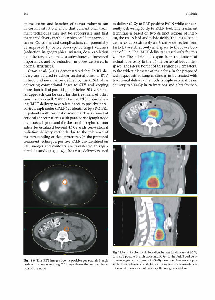
144 S. Mutic

of the extent and location of tumor volumes can in certain situations show that conventional treat-ment techniques may not be appropriate and that there are delivery methods which could improve out-comes. Outcomes and complications can potentially be improved by better coverage of target volumes (reduction in geographical misses), dose escalation to entire target volumes, or subvolumes of increased importance, and by reduction in doses delivered to normal structures.

Chao et al. (2001) demonstrated that IMRT de-livery can be used to deliver escalated doses to BTV in head and neck cancer defi ned by Cu-ATSM while delivering conventional doses to GTV and keeping more than half of parotid glands below 30 Gy. A simi-lar approach can be used for the treatment of other cancer sites as well. Mutic et al. (2003b) proposed us-ing IMRT delivery to escalate doses to positive para-aortic lymph nodes (PALN) as identifi ed by FDG-PET in patients with cervical carcinoma. The survival of cervical cancer patients with para-aortic lymph node metastases is poor, and the dose to this region cannot safely be escalated beyond 45 Gy with conventional radiation delivery methods due to the tolerance of the surrounding critical structures. In the proposed treatment technique, positive PALN are identifi ed on PET images and contours are transferred to regis-tered CT study (Fig. 11.8). The IMRT delivery is used

to deliver 60 Gy to PET-positive PALN while concur-rently delivering 50 Gy to PALN bed. The treatment technique is based on two distinct regions of inter-est, the PALN bed and pelvic fi elds. The PALN bed is defi ne as approximately an 8-cm-wide region from L4 to L5 vertebral body interspace to the lower bor-der of T12. The IMRT delivery is used only for this volume. The pelvic fi elds span from the bottom of ischial tuberosity to the L4–L5 vertebral body inter-space. The lateral border of this region is 1 cm lateral to the widest diameter of the pelvis. In the proposed technique, this volume continues to be treated with traditional delivery methods (simple external beam delivery to 50.4 Gy in 28 fractions and a brachyther-

Fig. 11.9a–c. A color-wash dose distribution for delivery of 60 Gy to a PET positive lymph node and 50 Gy to the PALN bed. Red-colored region corresponds to 60-Gy dose and blue area repre-sents doses between 50 and 60 Gy. a Transverse image orientation. b Coronal image orientation. c Sagittal image orientation

Fig. 11.8. This PET image shows a positive para-aortic lymph node and a corresponding CT image shows the mapped loca-tion of the node

b

a

c

PET and PET/CT for Radiotherapy Planning 145

apy boost (Grigsby et al. 2001a). Figure 11.9 shows a color-wash dose distribution for delivery of 60 Gy to a PET-positive lymph node and 50 Gy to the PALN bed. The red-colored region corresponds to 60-Gy dose and the blue area represents doses between 50 and 60 Gy. Esthappan et al. (2004) described in de-tail IMRT treatment-planning concerns for this de-livery technique.

Levivier et al. (2000) investigated potential ad-vantages of PET-guided gamma knife stereotactic radiosurgery. They were able to acquire acceptable stereotactic image registration accuracy with PET im-ages; however, they concluded that areas of increased FDG uptake were located predominantly within the MRI-defi ned tumor volumes and that PET provided little additional information. Gross et al. (1998) and Nuutinen et al. (2000) also concluded that PET con-tributes relatively small amount of additional infor-mation to MRI data for treatment of brain tumors. From these manuscripts it appears that PET may pro-vide useful information regarding boost volumes and it may allow differentiation of residual tumor better than MRI.

Mutic et al. (2002) and Malyapa et al. (2002) de-scribed FDG-PET based 3D brachytherapy treatment planning for treatment of cervical cancer. The pro-posed treatment technique was based on a postulate that FDG-PET images may allow a more accurate de-lineation of target volumes for brachytherapy gyne-cologic (GYN) implants. Both studies evaluated the feasibility of using PET as the sole source of target, normal structure, and applicator delineation for intra-cavitary GYN implant treatment planning. Standard Fletcher-Suit brachytherapy tandem and colpostat applicators which were used for radiation delivery can cause artifacts on CT and MR imaging and these imaging modalities require specialized applicators. In the proposed technique, after insertion of the appli-cators in the operating room, the patients were taken

to a PET scanner where 555 MBq (15 mCi) of 18F-FDG was intravenously administered. Forty-fi ve minutes later, three localization tubes containing 18F-FDG were inserted into the source afterloading compartments of the tandem and colpostat. A whole-pelvis scan was performed and the images were transferred to a com-mercial brachytherapy 3DTP system. A Foley catheter was also inserted into the urinary bladder while the patient was in the operating room. The regions of ra-dioactivity in the three applicator tubes on PET images were used to identify applicator locations. Tumor vol-ume, bladder, and rectum were also contoured on PET images. Figure 11.10 shows a PET image with three applicators, bladder, and rectum. From the contours, a 3D geometry of the implant, tumor volumes, and criti-cal structures was generated. Created treatment plans included dose-volume histograms (DVH) and 3D dose distribution displays.

Malyapa et al. (2002) compared PET-based GYN brachytherapy plans with conventional 2D treatment plans for 11 patients. They concluded that FDG-PET provides reliable estimate of the cervical cancer volume and 3D spatial relationship of the tumor to the tandem and ovoid applicators. There were no signifi cant differences in the calculated doses at the ICRU-38 defi ned point A, bladder, and rectum points between the conventional and proposed PET-based treatment-planning techniques. The maximum blad-der and rectal doses determined from the FDG-PET based dose-volume histograms were found to be higher than those obtained using conventional treat-ment planning. The PET-based treatment planning revealed that the ICRU reference point A isodose line did not cover all the tumors. The minimum dose to the tumor volume defi ned by FDG-PET ranged from 50 to 475 cGy for treatment plans designed to deliver 650 cGy to point A and exhibited an inverse correla-tion with tumor volume. The authors proposed that this technique has the potential for improving iso-

Fig. 11.10. A PET image of a patient with cervical carcinoma with inserted brachytherapy applicators

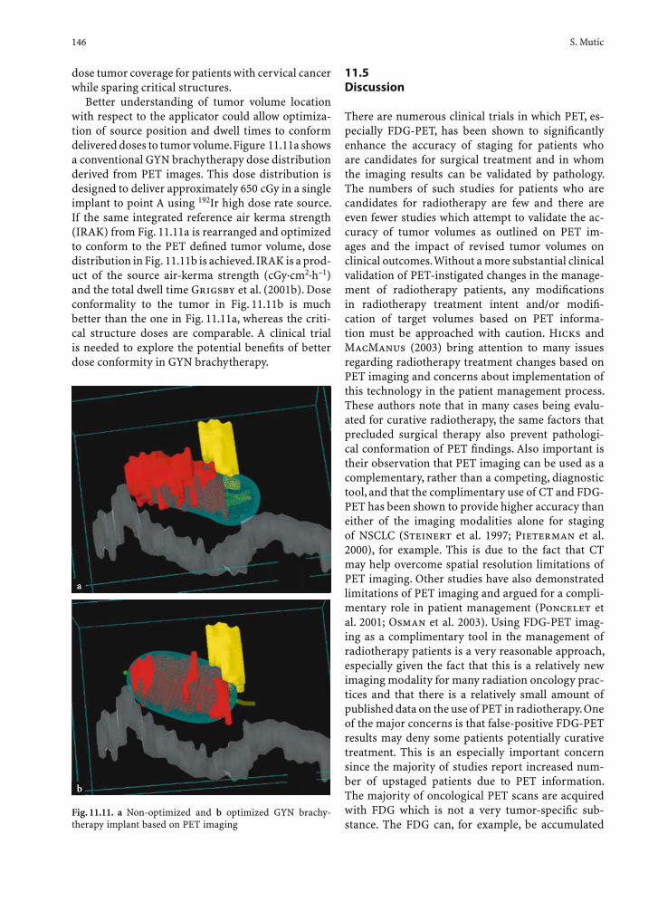
146 S. Mutic

dose tumor coverage for patients with cervical cancer while sparing critical structures.

Better understanding of tumor volume location with respect to the applicator could allow optimiza-tion of source position and dwell times to conform delivered doses to tumor volume. Figure 11.11a shows a conventional GYN brachytherapy dose distribution derived from PET images. This dose distribution is designed to deliver approximately 650 cGy in a single implant to point A using 192Ir high dose rate source. If the same integrated reference air kerma strength (IRAK) from Fig. 11.11a is rearranged and optimized to conform to the PET defi ned tumor volume, dose distribution in Fig. 11.11b is achieved. IRAK is a prod-uct of the source air-kerma strength (cGy·cm2·h–1) and the total dwell time Grigsby et al. (2001b). Dose conformality to the tumor in Fig. 11.11b is much better than the one in Fig. 11.11a, whereas the criti-cal structure doses are comparable. A clinical trial is needed to explore the potential benefi ts of better dose conformity in GYN brachytherapy.

11.5 Discussion

There are numerous clinical trials in which PET, es-pecially FDG-PET, has been shown to signifi cantly enhance the accuracy of staging for patients who are candidates for surgical treatment and in whom the imaging results can be validated by pathology. The numbers of such studies for patients who are candidates for radiotherapy are few and there are even fewer studies which attempt to validate the ac-curacy of tumor volumes as outlined on PET im-ages and the impact of revised tumor volumes on clinical outcomes. Without a more substantial clinical validation of PET-instigated changes in the manage-ment of radiotherapy patients, any modifi cations in radiotherapy treatment intent and/or modifi -cation of target volumes based on PET informa-tion must be approached with caution. Hicks and MacManus (2003) bring attention to many issues regarding radiotherapy treatment changes based on PET imaging and concerns about implementation of this technology in the patient management process. These authors note that in many cases being evalu-ated for curative radiotherapy, the same factors that precluded surgical therapy also prevent pathologi-cal conformation of PET fi ndings. Also important is their observation that PET imaging can be used as a complementary, rather than a competing, diagnostic tool, and that the complimentary use of CT and FDG-PET has been shown to provide higher accuracy than either of the imaging modalities alone for staging of NSCLC (Steinert et al. 1997; Pieterman et al. 2000), for example. This is due to the fact that CT may help overcome spatial resolution limitations of PET imaging. Other studies have also demonstrated limitations of PET imaging and argued for a compli-mentary role in patient management (Poncelet et al. 2001; Osman et al. 2003). Using FDG-PET imag-ing as a complimentary tool in the management of radiotherapy patients is a very reasonable approach, especially given the fact that this is a relatively new imaging modality for many radiation oncology prac-tices and that there is a relatively small amount of published data on the use of PET in radiotherapy. One of the major concerns is that false-positive FDG-PET results may deny some patients potentially curative treatment. This is an especially important concern since the majority of studies report increased num-ber of upstaged patients due to PET information. The majority of oncological PET scans are acquired with FDG which is not a very tumor-specifi c sub-stance. The FDG can, for example, be accumulated

Fig. 11.11. a Non-optimized and b optimized GYN brachy-therapy implant based on PET imaging

b

a

PET and PET/CT for Radiotherapy Planning 147

in benign lesions with elevated glucose metabolism, or there may be an increased accumulation in lymph nodes due to infl ammatory reaction rather than tu-mor presence, resulting in possibly false-positive fi ndings. The FDG uptake can be increased due to the effects of radiotherapy or chemotherapy, further complicating the evaluation of tumor location, shape, extent, and function. In order to accurately evalu-ate PET images, it is essential to understand various physiological uptake patterns of FDG for different cancer sites, and also to be aware of possibilities for false-positive and false-negative fi ndings (Strauss 1996; Cook et al. 1996). Numerous investigators have reported superiority of FDG-PET for staging and detection of many tumor sites. Inevitably, the majority of these reports also warn of false-positive fi ndings. Additionally, there are many studies which report possible sources of false-positive fi ndings for many cancer sites. The number of these reports far surpasses the number of papers describing the use of PET for radiotherapy treatment-planning purposes. The correlation of FDG uptake with anatomic abnor-malities detected by CT or MRI provides a valuable insight about functional and anatomical properties of a tumor. The PET/CT scanner and the availability of registered images simplifi es, to an extent, the vali-dation of PET fi ndings.

11.6 Conclusion

One great opportunity for an overall improvement of radiation oncology is better understanding of tu-mors through biological imaging. Biological imaging has been shown to better characterize the extent of disease than anatomical imaging and also to better characterize individual tumor properties. Enhanced understanding of individual tumors can improve se-lection of the most appropriate therapy and better defi nition of target volumes. Improved target vol-umes can utilize the full potential of IMRT delivery. Biological imaging can also allow evaluation of tu-mor response and possibly modifi cations in therapy plan, if the initial therapy is deemed not effective.

There are numerous biological imaging techniques under development which will allow improvement of radiotherapy; however, the main modality that cur-rently allows imaging beyond anatomy is FDG-PET. It is well established that PET imaging can signifi cantly affect management of cancer patients, including those that are candidates for radiotherapy. FDG-PET

has been shown to improve staging is several cancer sites. This improvement allows for more appropriate course of therapy for a signifi cant number of patients who would otherwise potentially undergo futile radi-cal therapy. This results in better quality of life for these patients and also health care costs reduction. Due to these benefi ts, the utilization of PET in oncol-ogy will only continue to grow.

It has been shown that PET can affect target vol-umes and result in delivery of escalated and more conformal dose distributions. It is unclear whether these modifi cations will result in improved tumor control and/or reduced side effects. Studies demon-strating positive impact of PET imaging in radio-therapy treatment planning process and meaningful improvement in target defi nition are needed to jus-tify modifi cation of conventional treatment volumes based on PET data.

The 18F-FDG is not a tumor-specifi c agent, there are numerous normal process and benign disease which can affect fi nding of PET imaging. Understanding of these process and potential for errors is imperative for implementation of FDG-PET imaging in radiotherapy treatment planning. The PET imaging will not benefi t all patients; therefore, it is important to have appro-priate selection process and timing of scans.

Other PET agents, many under development, have a potential to aid in achievement of some of the goals for this imaging modality in radiotherapy. The PET/CT combined scanner simplifi es this process and im-proves access to PET images for many radiation on-cology departments. Performance requirements for radiotherapy imaging are well defi ned and need to be applied to PET when used for treatment planning. Appropriate quality assurance program should also be implemented to avoid dosimetric and localization errors.

References

Bailey DL (2003) Data acquisition and performance charac-terization in PET. In: Valk PE, Bailey DL, Townsend DW, Maisey MN (eds) Positron emission tomography: basic science and clinical practice. Springer, Berlin Heidelberg New York, pp 69–90

Bailey DL, Karp JS, Surti S (2003) Physics and instrumentation in PET. In: Valk PE, Bailey DL, Townsend DW, Maisey MN (eds) Positron emission tomography: basic science and clinical practice. Springer, Berlin Heidelberg New York, pp 41–67

Beyer T, Townsend DW, Brun T, Kinahan PE, Charron M, Roddy R et al. (2000) A combined PET/CT scanner for clinical oncology. J Nucl Med 41:1369–1379

148 S. Mutic

Biehl K, Kong F, Bradley J, Dehdashti F, Mutic S, Siegel B (2004) FDG-PET defi nition of gross target volume for radiother-apy on NSCLC: is the use of 40% threshold appropriate? Cancer J 10 (Suppl 1):36

Bradley J, Thorstad WL, Mutic S, Miller TR, Dehdashti F, Siegel BA, Bosch W, Bertrand RJ (2004) Impact of FDG-PET on radiation therapy volume delineation in non-small-cell lung cancer. Int J Radiat Oncol Biol Phys 59:78–86

Chao KSC, Bosch WR, Mutic S, Lewis JS, Dehdashti F, Mintun MA, Dempsey JF, Perez CA, Purdy JA, Welch MJ (2001) A novel approach to overcome hypoxic tumor resistance Cu-ATSM-guided intensity-modulated radiation therapy. Int J Radiat Oncol Biol Phys 49:1171–1182

Cook GJ, Fogelman I, Maisey MN (1996) Normal physiological and benign pathological variations of 18-fl uoro-2-deoxy-glucose positron-emission tomography scanning: potential for error in interpretation. Semin Nucl Med 26:308–314

Defrise M, Kinahan PE, Michel C (2003) Image reconstruction algorithms in PET. In: Valk PE, Bailey DL, Townsend DW, Maisey MN (eds) Positron emission tomography: basic sci-ence and clinical practice. Springer, Berlin Heidelberg New York, pp 91–114

Dizendorf EV, Baumert BG, Schulthess GK von, Lutolf UM, Steinert HC (2003) Impact of whole-body 18F-FDG PET on staging and managing patients for radiation therapy. J Nucl Med 44:24–29

Erdi YE, Mawlawi O, Larson SM, Imbriaco M, Yeung H, Finn R, Humm JL (1997) Segmentation of lung lesion volume by adaptive positron emission tomography image threshold-ing. Cancer 80:2505–2509

Eshappan J, Mutic S, Malyapa RS, Grigsby PW, Zoberi I, Deh-dashti F, Miller TR, Bosch WR, Low DA (2004) Treatment planning guidelines regarding the use of CT/PET-guided IMRT for cervical carcinoma with positive para-aortic lymph nodes. Int J Radiat Oncol Biol Phys 58:1289–1297

Ezzel GA, Galvin JM, Low D, Palta JR, Rosen I, Sharpe MB, Xia P, Xiao Y, Xing L, Yu CX (2003) Guidance document on delivery, treatment planning, and clinical implementation of IMRT: report of the IMRT Subcommittee of the AAPM Radiation Therapy Committee. Med Phys 30:2089–2115

Gallagher BM, Fowler JS, Gutterson NI, MacGregor RR, Wan CN, Wolf AP (1978) Metabolic trapping as a principle of radiopharmaceutical design: some factors responsible for the biodistribution of [18F] 2-deoxy-2-fl uoro-D-glucose. J Nucl Med 10:1154–1161

Garcia-Ramirez JL, Mutic S, Dempsey JF, Low DA, Purdy JA (2002) Performance evaluation of an 85-cm bore X-ray computed tomography scanner designed for radiation oncology and comparison with current diagnostic CT scanners. Int J Radiat Oncol Biol Phys 52:1123–1131

Goitein M, Abrams M (1983) Multi-dimensional treatment planning I. Delineation of anatomy. Int J Radiat Oncol Biol Phys 9:777–787

Goitein M, Abrams M, Rowell D, Pollari H, Wiles J (1983) Multi-dimensional treatment planning II. Beam’s eye-view, back projection, and projection through CT sections. Int J Radiat Oncol Biol Phys 9:789–797

Grigsby PW, Perez CA, Chao KS, Herzog T, Mutch DG, Rader J (2001a) Radiation therapy for carcinoma of cervix with biopsy-proven positive para-aortic lymph nodes. Int J Radiat Oncol Biol Phys 49:733–738

Grigsby PW, Williamson JF, Chao KSC, Perez CA (2001b) Cer-vical tumor control evaluated with ICRU 38 reference vol-

umes an integrated reference air kerma. Radiother Oncol 58:10–23

Grigsby PW, Siegel BA, Dehdashti F, Mutch DG (2003) Post-therapy surveillance monitoring of cervical cancerr by FDG-PET. Int J Radiat Oncol Biol Phys 55:907–913

Gross MW, Weber WA, Feldman HJ, Bartenstein P, Schwaiger M, Molls M (1998) The value of F-18-fl uorodeoxyglucose PET for the 3-D radiation treatment planning for malig-nant gliomas. Int J Radiat Oncol Biol Phys 41:989–995

Hicks RJ, MacManus MP (2003) 18F-FDG PET in candidates for radiation therapy: Is it important and how do we vali-date its impact? J Nucl Med 44:30–32

Jerusalem G, Hustinx R, Beguin Y, Fillet G (2003) PET scan imaging in oncology. Eur J Cancer 39:1525–1534

Klingenbeck Regn K, Schaller S, Flohr T, Ohnesorge B, Kopp AF, Baum U (1999) Subsecond multi-slice computed tomogra-phy: basics and applications. Eur J Radiol 31:110–124

Lavely WC, Scarfone C, Cevikalp H, Rui L, Byrne DW, Cmelak AJ, Dawant B, Price RR, Hallahan DE, Fitzpatrick JM (2004) Phantom validation of coregistration of PET and CT for image-guided radiotherapy. Med Phys 31:1083–1092

Levivier M, Wikier D, Goldman S, David P, Matens T, Massager N, Gerosa M, Devriendt D, Desmedt F, Simon S, van Houtte P, Brotchi J (2000) Integration of the metabolic data of posi-tron emission tomography in the dosimetry planning of radiosurgery with the gamma knife: early experience with brain tumors. J Neurosurg 93:233–238

Ling CC, Humm J, Larson S, Amols H, Fuks Z, Leibel S, Koutcher JA (2000) Towards multidimensional radiotherapy (MD-CRT): biological imaging and biological conformality. Int J Radiat Oncol Biol Phys 47:551–560

Low DA, Nystrom M, Kalinin E, Parikh P, Dempsey JF, Bradley JD, Mutic S, Wahab SH, Islam T, Christensen G, Politte DG, Whiting BR (2003) A method for the reconstruction of 4-dimensional synchronized CT scans acquired during free breathing. Med Phys 30:1254–1263

MacManus MP, Hicks RJ, Ball DL, Kalff V, Matthews JP, Sal-minen E, Khaw P, Wirth A, Rischin D, McKenzie A (2001) F-18 Fluorodeoxyglucose positron emission tomography staging in radical radiotherapy candidates with nonsmall cell lung carcinoma. Cancer 92:886–895

Mah K, Caldwell CB, Ung YC, Danjoux CE, Balogh JM, Ganguli SN, Ehrlich LE, Tirona R (2002) The impact of 18FDG-PET on target and critical organs in CT-based treatment plan-ning of patients with poorly defi ned non-small cell lung carcinoma: a prospective study. Int J Radiat Oncol Biol Phys 52:339–350

Malyapa RS, Mutic S, Low DA, Zoberi I, Bosch WR, Miller TR, Grigsby PW (2002) Physiologic FDG-PET three dimen-sional brachytherapy treatment planning for cervical cancer. Int J Radiat Oncol Biol Phys 54:1140–1146

Meikle SR, Badawi RD (2003) Quantitative techniques in PET. In: Valk PE, Bailey DL, Townsend DW, Maisey MN (eds) Positron emission tomography: basic science and clinical practice. Springer, Berlin Heidelberg New York, pp 115–146

Miller TR, Grigsby PW (2002) Measurement of tumor volume by PET to evaluate prognosis in patients with advance cer-vical cancer treated by radiation therapy. Int J Radiat Oncol Biol Phys 53:353–359

Mutic S, Dempsey JF, Bosch WR, Low DA, Drzymala RE, Chao KSC, Goddu SM, Cutler PD, Purdy JA (2001) Multimodality image registration quality assurance for conformal three-

PET and PET/CT for Radiotherapy Planning 149

dimensional treatment planning. Int J Radiat Oncol Biol Phys 51:255–260

Mutic S, Grigsby PW, Low DA, Dempsey JF, Harms WR Sr, Laforest R, Bosch WR, Miller TR (2002) PET guided three-dimensional treatment planning of intracavitary gyneco-logic implants. Int J Radiat Oncol Biol Phys 52:1104–1110

Mutic S, Palta JR, Butker E, Das IJ, Huq MS, Loo LD, Salter BJ, McCollough CH, van Dyk J (2003a), Quality assurance for CT simulators and the CT simulation process: report of the AAPM Radiation Therapy Committee Task Group no. 66. Med Phys 30:2762–2792

Mutic S, Malyapa RS, Grigsby PW, Dehdashti F, Miller TR, Zoberi I, Bosch WR, Esthappan J, Low DA (2003b) PET-guided IMRT treatment for cervical carcinoma with posi-tive para-aortic lymph nodes: a dose escalation treatment planning study. Int J Radiat Oncol Biol Phys 55:28–35

National Electrical Manufacturers Association (NEMA) (1998) DICOM PS 3 (set). Digital Imaging Communictaions in Medicine (DICOM)

Nuutinen J, Sonninen P, Lehikoinen P, Sutinen E, Valavaara R, Eronen E, Norrgard S, Kulmala J, Teras M, Minn H (2000) Radiotherapy treatment planning and long-term follow-up with [(11)C]methionine PET in patients with low-grade astrocytoma, Int J Radiat Oncol Biol Phys 48:43–52

Osman MM, Cohade C, Nakamoto Y, Marshall LT, Leal JP, Wahl RL (2003) Clinically signifi cant inaccurate localization of lesions with PET/CT: frequency in 300 patients. J Nuc Med 44:240–243

Perez CA, Purdy JA, Harms W, Gerber R, Grahm MV, Matthews JW, Bosch W, Drzymala R, Emami B, Fox S (1995) Three-dimensional treatment planning and conformal radiation therapy: preliminary evaluation. Radiother Oncol 36:32–43

Pieterman, RM, van Putten JW, Meuzelaar JJ, Mooyaart EL, Vaalburg W, Koeter GH, Fidler V, Pruim J, Groen HJ (2000)

Preoperative staging of non-small-cell lung cancer with positron-emission tomography. N Engl J Med 343:254–261

Poncelet AJ, Lonneux M, Coche E, Weynand B, Noirhomme P (2001) PET-FDG enhances but does not replace preopera-tive surgical staging in non-small cell lung carcinoma. Eur J Cardiothorac Surg 20:468–474

Purdy JA (1997) Advances in three-dimensional treatment planning and conformal dose delivery. Semin Oncol 24:655–671

Sherouse GW, Novins K, Chaney EL (1990) Computation of digitally reconstructed radiographs for use in radiotherapy treatment design. Int J Radiat Oncol Biol Phys 18:651–658

Steinert HC, Hauser M, Allemann F, Engel H, Berthold T, Schulthess GK von, Weder W (1997) Non-small cell lung cancer: nodal staging with FDG PET versus CT with cor-relative lymph node mapping and sampling. Radiology 202:441–446

Strauss LG (2004) Fluorine-18 deoxygluocose and false-posi-tive results: a major problem in the diagnostics of oncologi-cal patients. Eur J Nucl Med 23:1409–1415

Townsend DW, Carney JP, Yap JT, Hall NC (2004) PET/CT today and tomorrow. J Nucl Med 45 (Suppl 1):4S–14S

Valk PE, Bailey DL, Townsend DW, Maisey MN (eds) (2002) Positron emission tomography: basic science and clinical practice. Springer, Berlin Heidelberg New York

Weissleder R, Mahmood U (2001) Melecular imaging. Radiol-ogy 219:316–333

Young H, Baum R, Cremerius U, Herholz K, Hoekstra O, Lam-mertsma AA, Pruim J, Price P (1999) Measurement of clini-cal and subclinical tumour response using [18F]-fl uorode-oxyglucose and positron emission tomography: review and 1999 EORTC recommendations. European Organization for Research and Treatment of Cancer (EORTC) PET Study Group. Eur J Cancer 13:1773–1782

Patient Positioning in Radiotherapy Using Optical-Guided 3D Ultrasound Techniques 151

12 Patient Positioning in Radiotherapy Using Optical-Guided 3D Ultrasound Techniques

Wolfgang A. Tomé, Sanford L. Meeks, Nigel P. Orton, Lionel G. Bouchet, and Mark A. Ritter

W.A. Tomé, PhD, Associate ProfessorN.P. Orton, PhD, Medical PhysicistM.A. Ritter, MD, PhD, Associate ProfessorDepartment of Human Oncology, University of Wisconsin Medical School, CSC K4/B100, 600 Highland Avenue, Madison, WI 53792, USAS.L. Meeks, PhDAssociate Professor, Department of Radiation Oncology, Room W189Z-GH, University of Iowa, 200 Hawkins Drive, Iowa City, IA 52242, USAL.G. Bouchet, PhDVice President, Technology Development, ZMed, Inc., Unit B-1, 200 Butterfi eld Drive, Ashland, MA 01721, USA

12.1 Introduction

Over the past decade, virtual simulation has become the standard of care for planning the majority of external beam radiotherapy treatments. There are many obvious technical advantages of virtual simu-lation over conventional radiotherapy simulation. Target identifi cation is more accurate, because the target may be identifi ed directly on CT and/or co-identifi ed on MRI, functional imaging scans, and PET

scans. Furthermore, the spatial relationship of the tumor to organs at risk is more easily appreciated in virtual simulation. This allows the treatment planner to tailor the beam orientations, fi eld sizes, and fi eld shapes to conformally avoid these organs at risk as far as possible. Further gains in conformal avoidance of organs at risk can usually be achieved when inverse planning is added to the treatment-planning arse-nal. Virtual simulation has provided the framework for 3D conformal therapy and intensity modulated radiotherapy.

While virtual simulation provides a signifi cant im-provement over conventional radiotherapy, the actual delivery of such virtually designed treatment plans has been limited by the accuracy of the fi ducial sys-tems traditionally chosen in radiotherapy. Optically guided radiotherapy systems have the potential for improving the precision of treatment delivery by providing more robust fi ducial systems. The ability of optically guided systems to accurately position internal targets with respect to the linear accelera-tor isocenter and to provide real-time patient track-ing enables one at least theoretically to signifi cantly reduce the amount of normal tissue included in the total irradiated volume by decreasing treatment fi eld margins. Implementation and correct use of such sys-tems present new challenges for the clinical physicist, and it is important that one thoroughly understands the strengths and weaknesses of such systems.

Furthermore, high-precision radiotherapy outside the cranium is challenging, because the target posi-tion can shift relative to bony anatomy between the time of initial image acquisition for virtual simula-tion and the time of the actual delivery of treatment. Our group has recently developed and clinically im-plemented an optically guided 3D ultrasound system for high-precision radiation delivery. The purpose of this chapter is to describe (a) optical ultrasound-guided radiotherapy, (b) the underlying mathematics that drive optical guidance, (c) the quality assurance techniques for such systems, and (d) the clinical use of optically guided 3D ultrasound patient position-ing systems.

CONTENTS

12.1 Introduction 15112.2 Optical Tracking 15212.3 Optically Guided 3D Ultrasound 15212.4 Mathematics of Optical Tracking and Ultrasound Calibration 15412.4.1 Mathematics of Optical Tracking 15412.4.2 Mathematics of Optical-Guided 3D Ultrasound Calibration 15512.4.2.1 Singular Value Decomposition 15612.4.2.2 Horn’s Algorithm 15612.5 Commissioning and Quality Assurance of 3D Ultrasound-Guided Systems 15712.6 Clinical Applications 159 References 163

152 W. A. Tomé et al.

12.2 Optical Tracking

Tracking is the process of measuring the location of instruments, anatomical structures, and/or land-marks in 3D space and in relationship to each other. Various technologies have been tested for determining an object’s location, including mechanical, magnetic, acoustic, inertial, and optical position sensors. Most of these technologies have been tested for medical use in either image-guided surgery or image-guided tracking in radiation therapy.

Optical tracking systems use infrared light to deter-mine a target’s position. The target may either be active or passive. The most common active targets are infra-red light emitting diodes (IRLED). Passive targets are generally spheres or disks coated with a highly refl ec-tive material that refl ects infrared light from an external source. Various detectors can be used to determine the positions of an optical target; however, charged couple device (CCD) cameras are used most often. The CCD cameras are simply a collection of light sensitive cells, or pixels, arranged in either a one- or two-dimensional array. When light strikes a CCD cell, electron produc-tion is proportional to the intensity of the light incident on the cell; thus, a 2D CCD array provides a 2D digital “image” of the target, with brighter pixels in the array corresponding to a higher light intensity and darker pixels corresponding to lower light intensity. This digi-tal image can then be analyzed to determine the pixel with the highest light intensity. Each camera in a 2D CCD array determines a ray in 3D. If two 2D CCDs are used in the camera of an optical tracking system, the intersection of the two 2D rays emanating form the CCDs determines a line in 3D space, whereas if three 2D CCDs are used, the intersection of all three 2D rays determines a point in 3D space.

12.3 Optically Guided 3D Ultrasound

In extracranial radiotherapy, soft tissue targets can move relative to bony anatomy between the time of image acquisition for treatment planning and the time of the actual treatment delivery; therefore, real-time imaging of internal anatomy is required in extracra-nial radiotherapy if one would like to accurately local-ize a target at the time of treatment delivery. We have developed and tested an optical-guided system for 3D ultrasound guidance (Bouchet et al. 2001; Bouchet et al. 2002; Meeks et al. 2003; Ryken et al. 2001; Tomé

et al. 2002) that is commercially available under the trade name SonArray (ZMed, Inc., Ashland, Mass.). Ultrasound was chosen because it is an inexpensive, yet fl exible and high-resolution imaging modality that can easily be adapted for use in a radiation therapy treatment room. Systems have been developed that rely on 2D ultrasound probes attached to mechani-cal tracking systems, and these have proved effective for improving the precision of patient localization for prostate radiotherapy (Troccaz et al. 1995; Lattanzi et al. 1999; Lattanzi et al. 2000). The interpretation of 2D ultrasound images, however, is diffi cult and can be highly dependent on the skill and expertise of the operator in manipulating the transducer and mentally transforming the 2D images into a 3D tissue structure. In principle, the use of 3D ultrasound can help over-come this limitation, but the relatively high cost of true 3D ultrasound devices has prohibited their use in radiotherapy for target localization on a routine basis; however, the development of our optical-guided 3D ultrasound target localization system has decreased the cost of such a system to a level that is compa-rable to commercially available 2D ultrasound target localization systems, and has therefore led to a more widespread use of reconstructed 3D Ultrasound for target localization in radiotherapy. The 3D ultrasound data sets are generated through optically tracking the acquisition of free-hand 2D ultrasound images. The operator holds the ultrasound probe and manipulates it over the anatomical region of interest. The raw 2D ultrasound images are transferred to a workstation using a standard video link. During acquisition, the position and angulation of each 2D ultrasound image is determined form the position and angulation of the 2D ultrasound probe by optically tracking a rigidly at-tached active fi ducial array that has four infrared light-emitting diodes (IRLEDs; see Fig. 12.1). The position of each ultrasound pixel can therefore be determined, and an ultrasound volume can be reconstructed by coupling the position information obtained through optical tracking with the raw ultrasound data (see Figs. 12.2, 12.3).

Therefore, in addition to building the 3D image volume, optical guidance is also used to determine the absolute position of the ultrasound volume in the treatment room coordinate system. Because the rela-tive positions of the ultrasound volume and the ultra-sound probe are fi xed, the knowledge of the probe position in the treatment room coordinate system at the time of image acquisition is suffi cient to determine the position of the image volume relative to the lin-ear accelerator isocenter. The relative position of the image and probe is determined during a calibration

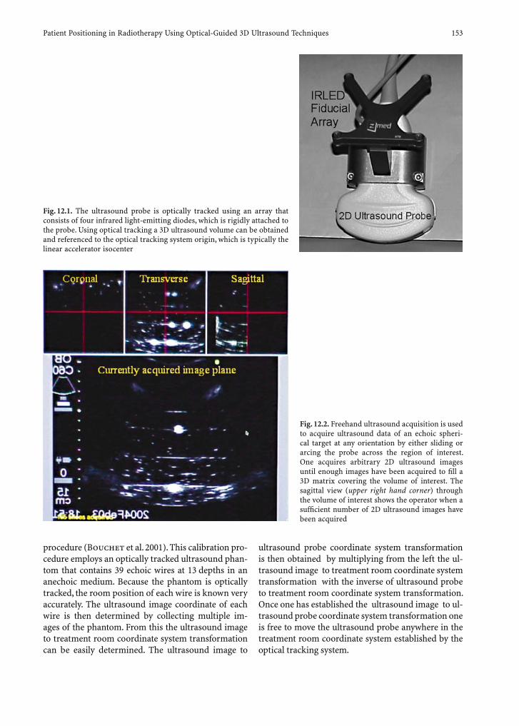
Patient Positioning in Radiotherapy Using Optical-Guided 3D Ultrasound Techniques 153

procedure (Bouchet et al. 2001). This calibration pro-cedure employs an optically tracked ultrasound phan-tom that contains 39 echoic wires at 13 depths in an anechoic medium. Because the phantom is optically tracked, the room position of each wire is known very accurately. The ultrasound image coordinate of each wire is then determined by collecting multiple im-ages of the phantom. From this the ultrasound image to treatment room coordinate system transformation can be easily determined. The ultrasound image to

Fig. 12.1. The ultrasound probe is optically tracked using an array that consists of four infrared light-emitting diodes, which is rigidly attached to the probe. Using optical tracking a 3D ultrasound volume can be obtained and referenced to the optical tracking system origin, which is typically the linear accelerator isocenter

Fig. 12.2. Freehand ultrasound acquisition is used to acquire ultrasound data of an echoic spheri-cal target at any orientation by either sliding or arcing the probe across the region of interest. One acquires arbitrary 2D ultrasound images until enough images have been acquired to fi ll a 3D matrix covering the volume of interest. The sagittal view (upper right hand corner) through the volume of interest shows the operator when a suffi cient number of 2D ultrasound images have been acquired

ultrasound probe coordinate system transformation is then obtained by multiplying from the left the ul-trasound image to treatment room coordinate system transformation with the inverse of ultrasound probe to treatment room coordinate system transformation. Once one has established the ultrasound image to ul-trasound probe coordinate system transformation one is free to move the ultrasound probe anywhere in the treatment room coordinate system established by the optical tracking system.

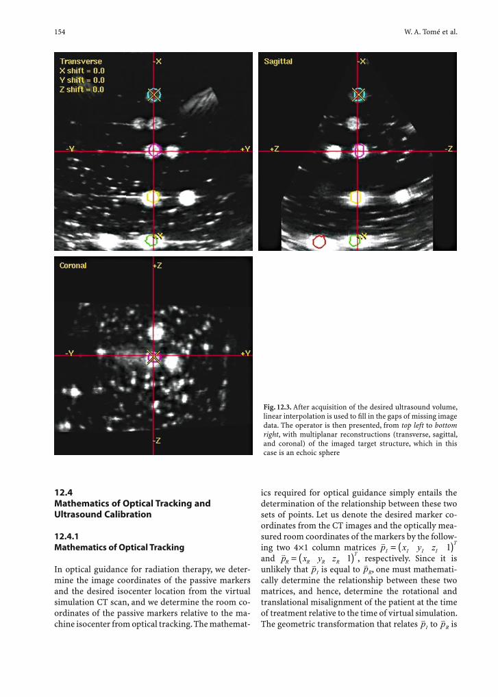
154 W. A. Tomé et al.

12.4 Mathematics of Optical Tracking and Ultrasound Calibration

12.4.1 Mathematics of Optical Tracking

In optical guidance for radiation therapy, we deter-mine the image coordinates of the passive markers and the desired isocenter location from the virtual simulation CT scan, and we determine the room co-ordinates of the passive markers relative to the ma-chine isocenter from optical tracking. The mathemat-

ics required for optical guidance simply entails the determination of the relationship between these two sets of points. Let us denote the desired marker co-ordinates from the CT images and the optically mea-sured room coordinates of the markers by the follow-ing two 4¥1 column matrices p x( )v y zI I I I

T= 1 and p x( )v y zR R R R

T= 1 , respectively. Since it is unlikely that

vpI is equal to vpR, one must mathemati-

cally determine the relationship between these two matrices, and hence, determine the rotational and translational misalignment of the patient at the time of treatment relative to the time of virtual simulation. The geometric transformation that relates

vpI to vpR is

Fig. 12.3. After acquisition of the desired ultrasound volume, linear interpolation is used to fi ll in the gaps of missing image data. The operator is then presented, from top left to bottom right, with multiplanar reconstructions (transverse, sagittal, and coronal) of the imaged target structure, which in this case is an echoic sphere

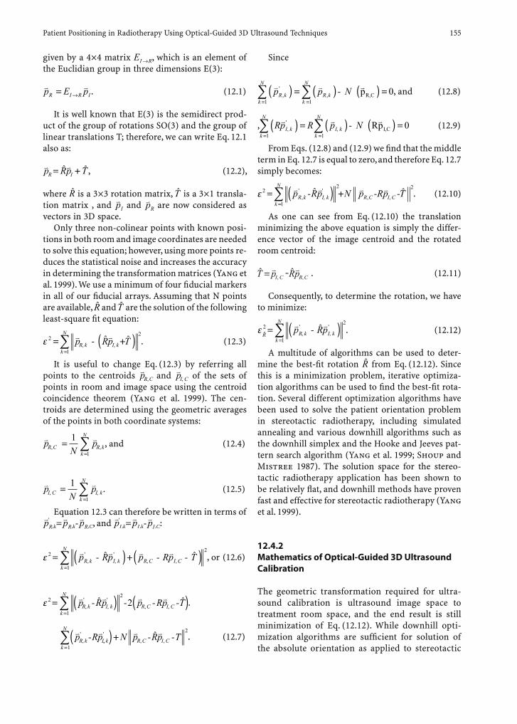
Patient Positioning in Radiotherapy Using Optical-Guided 3D Ultrasound Techniques 155

given by a 4¥4 matrix EI R→ , which is an element of the Euclidian group in three dimensions E(3):

v vp E pR I R I= → . (12.1)

It is well known that E(3) is the semidirect prod-uct of the group of rotations SO(3) and the group of linear translations T; therefore, we can write Eq. 12.1 also as:

= +v vp Rp TR Iˆ ˆ , (12.2),

where R is a 3¥3 rotation matrix, T is a 3¥1 transla-tion matrix , and

vpI and vpR are now considered as

vectors in 3D space.Only three non-colinear points with known posi-

tions in both room and image coordinates are needed to solve this equation; however, using more points re-duces the statistical noise and increases the accuracy in determining the transformation matrices (Yang et al. 1999). We use a minimum of four fi ducial markers in all of our fi ducial arrays. Assuming that N points are available, R and T are the solution of the following least-square fi t equation:

v v 2p T( ), ,R kε 2

1= − +

=∑ p Rk

N

I kˆ ˆ . (12.3)

It is useful to change Eq. (12.3) by referring all points to the centroids ,

vpR C and vpI C, of the sets of

points in room and image space using the centroid coincidence theorem (Yang et al. 1999). The cen-troids are determined using the geometric averages of the points in both coordinate systems:

, ,v vp

NpR C R k

k

N

==

∑11

, and (12.4)

v vpN

pI C I kk

N

, ,==

∑11

. (12.5)

Equation 12.3 can therefore be written in terms of vpR

',k=

vpR,k-vpR,C, and

vpI'

,k=vpI ,k-

vpI ,C:

ε 22

1= −( )+ − −( )

=∑ v v v vp Rp p Rp TR k I k R C I Ck

N

,'

,'

, ,ˆ ˆ , or (12.6)

( ), ,− −p pv v= −ε 22

12( ) −

=∑ v vp R Rp TR k I kk

N

R C I C,'

,'ˆ ˆ .

( )−v vp RpR k I,'

,,'

, ,kk

N

R C I CN p Rp T+ − −=

∑1

2v vˆ . (12.7)

Since

( )v v vp p NR kk

N

R kk

N

,'

,( ) = − ( ) == =

∑ ∑1 1

0 pR,C , and (12.8)

, ( )∑ ∑( )Rp R p NI kk

N

I kk

Nv v v,

',= − ( ) =

= =1 10 RpI,C (12.9)

From Eqs. (12.8) and (12.9) we fi nd that the middle term in Eq. 12.7 is equal to zero, and therefore Eq. 12.7 simply becomes:

p Rp N( )v v= −ε 22

1

2+ − −

=∑ v vp R p TR k I kk

N

R C I C,'

,'

, ,ˆ ˆ . (12.10)

As one can see from Eq. (12.10) the translation minimizing the above equation is simply the differ-ence vector of the image centroid and the rotated room centroid:

. (12.11)

Consequently, to determine the rotation, we have to minimize:

= −v v( )R kε ,'

,'

R I kk

N

p Rp22

1=∑ˆ

ˆ . (12.12)

A multitude of algorithms can be used to deter-mine the best-fi t rotation R from Eq. (12.12). Since this is a minimization problem, iterative optimiza-tion algorithms can be used to fi nd the best-fi t rota-tion. Several different optimization algorithms have been used to solve the patient orientation problem in stereotactic radiotherapy, including simulated annealing and various downhill algorithms such as the downhill simplex and the Hooke and Jeeves pat-tern search algorithm (Yang et al. 1999; Shoup and Mistree 1987). The solution space for the stereo-tactic radiotherapy application has been shown to be relatively fl at, and downhill methods have proven fast and effective for stereotactic radiotherapy (Yang et al. 1999).

12.4.2 Mathematics of Optical-Guided 3D Ultrasound Calibration

The geometric transformation required for ultra-sound calibration is ultrasound image space to treatment room space, and the end result is still minimization of Eq. (12.12). While downhill opti-mization algorithms are suffi cient for solution of the absolute orientation as applied to stereotactic

156 W. A. Tomé et al.

radiotherapy, additional noise from ultrasound im-aging decreases the reliability of these simple algo-rithms for determining the ultrasound calibration matrix (Bouchet et al. 2001). Below are brief dis-cussions of two closed-form solutions algorithms (the singular value decomposition algorithm and Horn’s algorithm using quaternions) to the absolute orientation problem.

12.4.2.1 Singular Value Decomposition

The minimum of Eq. 12.12 is achieved when for all k Π{1, ..., N},we have

v vp RpR k I k,'

,'= ˆ . This can be rewrit-

ten in terms of a simple matrix equation:

Z Z, ,

, ,

, ,

I I

I I

1 2

I I1 2

1 2R N

R N

R N

, ,

R R, ,1 2

1 2

1 2

X X XY Y YZ Z Z

R R

R R

,

,

, , ,

....

....

....

⎡

⎣

⎢⎢⎢

⎤

⎦

⎥⎥⎥

=⎡

⎣

⎢⎢⎢

⎤............

,

,

,

RX X XY Y Y

Z

I N

I N

I N⎦

⎥⎥⎥

ˆ ,(12.13)

where (X, Y, Z) represent the Cartesian coordinates of the points p. Equation (12.13) represents an over-determined linear set of equations that can be solved by using the singular value decomposition theorem. This theorem yields the decomposition of the result-ing N×3 matrix into a product matrices of the form UWVT where U,V are orthogonal matrices and W is a diagonal matrix whose diagonal elements are either positive or zero. After decomposition, the solution of Eq. (12.13) can be determined by inverting the cor-responding orthogonal matrices. This closed-form solution gives the rotation that minimizes the least-square problem stated in Eq. (12.12).

12.4.2.2 Horn’s Algorithm

Another algorithm that can be used to solve Eq. (12.12) is the closed-form solution presented by Horn using quaternion theory (Horn 1987; Bouchet et al. 2001). Quaternions are an exten-sion of complex numbers. Instead of just i, one has three different numbers that are all square roots of –1 labeled i, j, and k, that fulfi ll the following relationship:

i j kijk� =ε ,

where ijkε , is the totally antisymmetric tensor. The conjugate and the magnitude of a quaternion are formed in much the same way as the complex conju-gate and magnitude:

&q q iq jq kqx y z= + + +0 ,

q q&′ = − − −iq jq kqx y z0

& & &q q q q q q qx y z= � ′ = + + +02 2 2 2 (12.14)

In what follows we only between will and deal with unit quaternions, i.e., quaternions for which &q 1= . For unit quaternions the inverse of a quaternion is equal to its conjugate. Since unit quaternions form a representation of the special unitary group SU(2) one can express any 3D rotation R in terms of unit quaternions using the following isomorphism:

r r q r= → = �r r

& & & &r R q1 0 1 0 � ′, (12.15)

Expanding Eq. (12.12) and using the fact that ro-tations are isomorphisms, i.e., leave the norm un-changed, one fi nds:

v v∑ ∑− ⋅ I kR k= + I kR k= =

ε ,'

,'

,'

,'

Rk

N

k

N

k

N

p p p Rp2 2 2

112

=∑v v

ˆ1

ˆ .

(12.16)

Therefore, minimizing Eq. (12.16) corresponds to maximizing the last term in this expression since the fi rst two terms of this expression are positively defi -nite:

∑ ∑p Rξ = ⋅ = ⋅=

v v v vp R p pR k I kk

N

I k R kk

N

,'

,'

,'

,'

1 1=

ˆ ˆ , (12.17)

which can be written in terms of quaternions using the isomorphism (Eq. (12.15)) as follows:

, ,& &q p= �ξ � ′�=

∑ & &q pI k R kk

N

1.

(12.18)

Using the fact that there exists a matrix represen-tation of quaternion multiplication, Eq. (12.18) can be rewritten as (cf. Horn (1987):

ξ= qNqT, (12.19)

where N Nkk

N==∑ 1

is a 4×4 matrix formed from the coordinates of the points

vpI k, and vpR k, and the unit

quaternion q is represented as a row vector of the form q q q q qx y z o= ( , ), , . Horn (1987) has shown that the unit quaternion maximizing Eq. (12.19) is the eigenvector corresponding to the largest positive eigenvalue of the matrix N. Since N is a 4×4 matrix, this corresponds to fi nding the roots of the fourth-degree characteristic polynomial of N. This unit quaternion corresponds to the closed-form solution of the rotation minimizing the least-square problem stated in Eq. (12.12).

&q

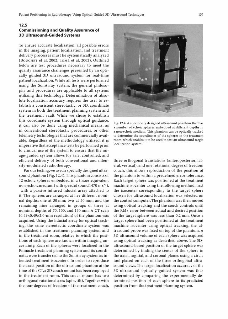
Patient Positioning in Radiotherapy Using Optical-Guided 3D Ultrasound Techniques 157

12.5 Commissioning and Quality Assurance of 3D Ultrasound-Guided Systems

To ensure accurate localization, all possible errors in the imaging, patient localization, and treatment delivery processes must be systematically analyzed (Bouchet et al. 2002; Tomé et al. 2002). Outlined below are test procedures necessary to meet the quality assurance challenges presented by an opti-cally guided 3D ultrasound system for real-time patient localization. While all tests were performed using the SonArray system, the general philoso-phy and procedures are applicable to all systems utilizing this technology. Determination of abso-lute localization accuracy requires the user to es-tablish a consistent stereotactic, or 3D, coordinate system in both the treatment planning system and the treatment vault. While we chose to establish this coordinate system through optical guidance, it can also be done using mechanical means, as in conventional stereotactic procedures, or other telemetry technologies that are commercially avail-able. Regardless of the methodology utilized, it is imperative that acceptance tests be performed prior to clinical use of the system to ensure that the im-age-guided system allows for safe, controlled, and effi cient delivery of both conventional and inten-sity-modulated radiotherapy.

For our testing, we used a specially designed ultra-sound phantom (Fig. 12.4). This phantom consists of 12 echoic spheres embedded in a tissue-equivalent non-echoic medium (with speed of sound 1470 m s-1), with a passive infrared fi ducial array attached to it. The spheres are arranged at fi ve different nomi-nal depths: one at 30 mm; two at 50 mm; and the remaining nine arranged in groups of three at nominal depths of 70, 100, and 130 mm. A CT scan (0.49×0.49×2.0-mm resolution) of the phantom was acquired. Using the fi ducial array for optical track-ing, the same stereotactic coordinate system was established in the treatment planning system and in the treatment room, relative to which the posi-tions of each sphere are known within imaging un-certainty. Each of the spheres were localized in the Pinnacle treatment planning system and its coordi-nates were transferred to the SonArray system as in-tended treatment isocenters. In order to reproduce the exact position of the ultrasound phantom at the time of the CT, a 2D couch mount has been employed in the treatment room. This couch mount has two orthogonal rotational axes (spin, tilt). Together with the four degrees of freedom of the treatment couch,

three orthogonal translations (anteroposterior, lat-eral, vertical), and one rotational degree of freedom couch, this allows reproduction of the position of the phantom to within a predefi ned error tolerance. Each target sphere was positioned at the treatment machine isocenter using the following method: fi rst the isocenter corresponding to the target sphere chosen for ultrasound localization was selected on the control computer. The phantom was then moved using optical tracking and the couch controls until the RMS error between actual and desired position of the target sphere was less than 0.2 mm. Once a target sphere had been positioned at the treatment machine isocenter using optical tracking, the ul-trasound probe was fi xed on top of the phantom. A 3D ultrasound volume of each sphere was acquired using optical tracking as described above. The 3D-ultrasound-based position of the target sphere was determined by fi nding the center of the sphere in the axial, sagittal, and coronal planes using a circle tool placed on each of the three orthogonal ultra-sound views. The target localization accuracy of the 3D-ultrasound optically guided system was thus determined by comparing the experimentally de-termined position of each sphere to its predicted position from the treatment planning system.

Fig. 12.4. A specifi cally designed ultrasound phantom that has a number of echoic spheres embedded at different depths in a non-echoic medium. This phantom can be optically tracked to determine the coordinates of the spheres in the treatment room, which enables it to be used to test an ultrasound target localization system.

158 W. A. Tomé et al.

Our data show that the localization error does not depend on the target depth or the ultrasound focal depth used. Table 12.1 demonstrates representative values for such a test of optically guided 3D-ultra-sound target localization for a 15-cm depth ultra-sound probe format, which is the typical depth one employs in ultrasound localizations of the prostate. Similar to optical guidance testing described previ-ously, optically guided 3D-ultrasound localization should be able to localize a well-defi ned internal tar-get to within the inherent imaging uncertainty; how-ever, localization errors in each of the spatial dimen-sions may exceed the predicted localization error due to fi nite image pixel size.

Other experiments can be performed using an-thropomorphic phantoms. As an example we de-scribe below an experiment using a specially de-signed prostate phantom. This prostate phantom consists of three layers. The fi rst layer contains a model of the bladder, the second a model of the pros-tate and urethra, and the third a model for the rectum in the form of a long cylinder. The bladder, prostate, urethra, rectum, and the background material are made of Zerdine with different echogenicity closely mimicking sound absorption and speed properties characteristic for these anatomical structures. A CT scan (0.49×0.49×2.0-mm resolution) of the phantom with a passive infrared fi ducial array attached was acquired. Using optical tracking as described previ-ously, the positions of each organ can be determined in both CT image space and treatment room space within imaging uncertainty. In the CT data set four distinct regions of interest (ROIs) – bladder, prostate, urethra, and rectum – were segmented. A treatment isocenter was chosen in the treatment planning sys-tem, and the planning CT, isocenter, and segmented ROIs were transferred to the control computer of the 3D-ultrasound target localization system. The phan-tom was then set up on the treatment couch as shown in Fig. 12.5.

Again, optical tracking can be used to align the planned treatment isocenter with the treatment machine isocenter within 0.2 mm RMS error. The fi ducial array attached to the phantom is then cov-ered and a separate fi ducial array is attached to the treatment couch, and the position of this second ar-ray is recorded using the optical positioning sensor system. In this way a fi xed “bony anatomy” is estab-lished about which introduced internal organ mo-tion can be simulated as follows: fi rst the fi ducial ar-ray attached to treatment couch is covered and the fi ducial array attached to the phantom is uncovered. Then the phantom is shifted from its starting posi-

tion ±5 mm in the lateral and/or superior/inferior directions using a 2D translation table. These shifts are measured to within ±0.2 mm RMS error using the optical positioning sensor system. Once the shifts have been made, the fi ducial array attached to the phantom is again covered and the fi ducial ar-ray attached to the treatment couch is uncovered. Since the treatment couch position remains fi xed, the “bony anatomy” is not changed, even though the phantom has been physically moved; hence, through the alternate use of two fi ducial arrays one is able to introduce accurate apparent organ motion while maintaining a fi xed “bony anatomy.” This apparent organ motion can then be detected using optically guided 3D ultrasound imaging by employing the op-tically guided 3D ultrasound target localization sys-

Table 12.1. Accuracy of optically guided 3D ultrasound as a function of the depth of the target for a focal depth of 15 cm. Results are given in terms of the mean distance in the antero-posterior, lateral, and axial directions and the 95% confi dence interval around that mean value

Depth (mm)

Anteroposterior distance (mm)

Lateral distance (mm)

Axial distance (mm)

30 0.8±0.6 0.5±0.3 1.0±1.7

50 0.1±0.7 0.6±0.8 1.3±1.6

70 -0.2±0.6 1.0±0.9 0.1±1.5

100 0.2±0.8 1.2±0.9 0.3±1.8

130 0.3±0.6 1.1±1.0 0.2±1.5

Fig. 12.5. Experimental setup of the prostate phantom in the treatment room for determining unknown induced motion in a target structure using an ultrasound target localization system

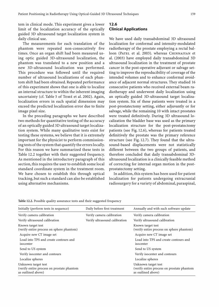
Patient Positioning in Radiotherapy Using Optical-Guided 3D Ultrasound Techniques 159

tem in clinical mode. This experiment gives a lower limit of the localization accuracy of the optically guided 3D ultrasound target localization system in daily clinical use.

The measurements for each translation of the phantom were repeated non-consecutively fi ve times. Once an organ shift had been measured us-ing optic guided 3D-ultrasound localization, the phantom was translated to a new position and a new 3D-ultrasound localization was performed. This procedure was followed until the required number of ultrasound localizations of each phan-tom shift had been obtained. Repeated performance of this experiment shows that one is able to localize an internal structure to within the inherent imaging uncertainty (cf. Table 5 of Tomé et al. 2002). Again, localization errors in each spatial dimension may exceed the predicted localization error due to fi nite image pixel size.

In the preceding paragraphs we have described two methods for quantitative testing of the accuracy of an optically guided 3D ultrasound target localiza-tion system. While many qualitative tests exist for testing these systems, we believe that it is extremely important for the physicist to perform commission-ing tests of the system that quantify the errors locally. For this reason we have summarized these tests in Table 12.2 together with their suggested frequency. As mentioned in the introductory paragraph of this section, this requires the user to establish some local standard coordinate system in the treatment room. We have chosen to establish this through optical tracking, but such a standard can also be established using alternative mechanisms.

12.6 Clinical Applications

We have used daily transabdominal 3D ultrasound localization for conformal and intensity-modulated radiotherapy of the prostate employing a rectal bal-loon (Patel et al. 2003). whereas Chinnaiyan et al. (2003) have employed daily transabdominal 3D ultrasound localization in the treatment of prostate cancer in the post-operative adjuvant or salvage set-ting to improve the reproducibility of coverage of the intended volumes and to enhance conformal avoid-ance of adjacent normal structures. They studied 16 consecutive patients who received external beam ra-diotherapy and underwent daily localization using an optically guided 3D-ultrasound target localiza-tion system. Six of these patients were treated in a post-prostatectomy setting, either adjuvantly or for salvage, while the remaining 10 with intact prostates were treated defi nitively. During 3D ultrasound lo-calization the bladder base was used as the primary localization structure for the post-prostatectomy patients (see Fig. 12.6), whereas for patients treated defi nitively the prostate was the primary reference structure (see Fig. 12.7). They found that the ultra-sound-based displacements were not statistically different between the two groups of patients, and therefore concluded that daily transabdominal 3D-ultrasound localization is a clinically feasible method of correcting for internal organ motion in the post-prostatectomy setting.

In addition, this system has been used for patient localization for patients undergoing extracranial radiosurgery for a variety of abdominal, paraspinal,

Table 12.2. Possible quality assurance tests and their suggested frequency

Initially (perform tests in sequence) Daily before fi rst treatment Annually and with each software update

Verify camera calibration Verify camera calibration Verify camera calibration

Verify ultrasound calibration Verify ultrasound calibration Verify ultrasound calibration

Known target test (verify entire process on sphere phantom)

Known target test (verify entire process on sphere phantom)

Acquire new CT image set Acquire new CT image set

Load into TPS and create contours and isocenter

Load into TPS and create contours and isocenter

Send to US system Send to US system

Verify isocenter and contours Verify isocenter and contours

Localize spheres Localize spheres

Unknown target test (verify entire process on prostate phantom as outlined above)

Unknown target test (verify entire process on prostate phantom as outlined above)

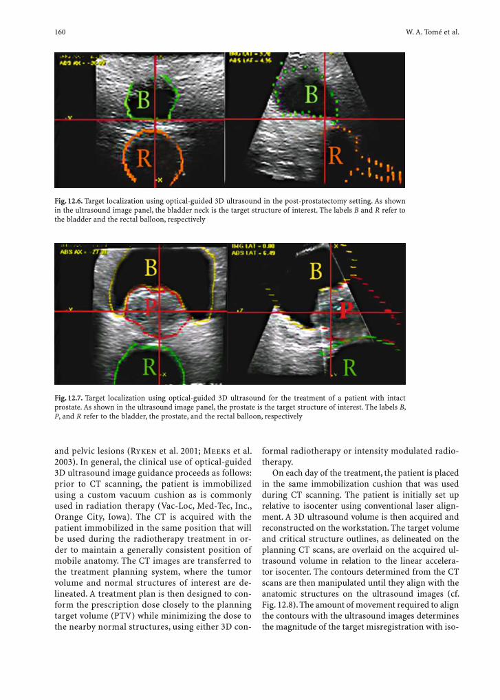
160 W. A. Tomé et al.

and pelvic lesions (Ryken et al. 2001; Meeks et al. 2003). In general, the clinical use of optical-guided 3D ultrasound image guidance proceeds as follows: prior to CT scanning, the patient is immobilized using a custom vacuum cushion as is commonly used in radiation therapy (Vac-Loc, Med-Tec, Inc., Orange City, Iowa). The CT is acquired with the patient immobilized in the same position that will be used during the radiotherapy treatment in or-der to maintain a generally consistent position of mobile anatomy. The CT images are transferred to the treatment planning system, where the tumor volume and normal structures of interest are de-lineated. A treatment plan is then designed to con-form the prescription dose closely to the planning target volume (PTV) while minimizing the dose to the nearby normal structures, using either 3D con-

formal radiotherapy or intensity modulated radio-therapy.

On each day of the treatment, the patient is placed in the same immobilization cushion that was used during CT scanning. The patient is initially set up relative to isocenter using conventional laser align-ment. A 3D ultrasound volume is then acquired and reconstructed on the workstation. The target volume and critical structure outlines, as delineated on the planning CT scans, are overlaid on the acquired ul-trasound volume in relation to the linear accelera-tor isocenter. The contours determined from the CT scans are then manipulated until they align with the anatomic structures on the ultrasound images (cf. Fig. 12.8). The amount of movement required to align the contours with the ultrasound images determines the magnitude of the target misregistration with iso-

Fig. 12.7. Target localization using optical-guided 3D ultrasound for the treatment of a patient with intact prostate. As shown in the ultrasound image panel, the prostate is the target structure of interest. The labels B, P, and R refer to the bladder, the prostate, and the rectal balloon, respectively

Fig. 12.6. Target localization using optical-guided 3D ultrasound in the post-prostatectomy setting. As shown in the ultrasound image panel, the bladder neck is the target structure of interest. The labels B and R refer to the bladder and the rectal balloon, respectively

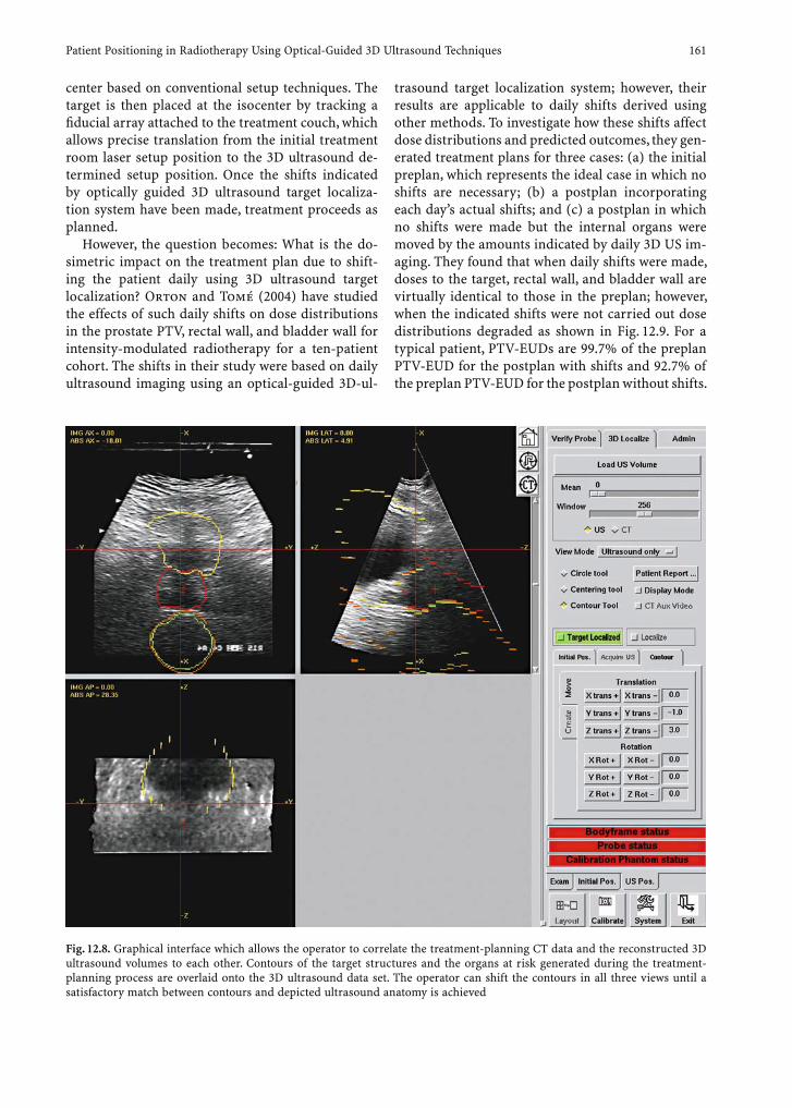
Patient Positioning in Radiotherapy Using Optical-Guided 3D Ultrasound Techniques 161

center based on conventional setup techniques. The target is then placed at the isocenter by tracking a fi ducial array attached to the treatment couch, which allows precise translation from the initial treatment room laser setup position to the 3D ultrasound de-termined setup position. Once the shifts indicated by optically guided 3D ultrasound target localiza-tion system have been made, treatment proceeds as planned.

However, the question becomes: What is the do-simetric impact on the treatment plan due to shift-ing the patient daily using 3D ultrasound target localization? Orton and Tomé (2004) have studied the effects of such daily shifts on dose distributions in the prostate PTV, rectal wall, and bladder wall for intensity-modulated radiotherapy for a ten-patient cohort. The shifts in their study were based on daily ultrasound imaging using an optical-guided 3D-ul-

trasound target localization system; however, their results are applicable to daily shifts derived using other methods. To investigate how these shifts affect dose distributions and predicted outcomes, they gen-erated treatment plans for three cases: (a) the initial preplan, which represents the ideal case in which no shifts are necessary; (b) a postplan incorporating each day’s actual shifts; and (c) a postplan in which no shifts were made but the internal organs were moved by the amounts indicated by daily 3D US im-aging. They found that when daily shifts were made, doses to the target, rectal wall, and bladder wall are virtually identical to those in the preplan; however, when the indicated shifts were not carried out dose distributions degraded as shown in Fig. 12.9. For a typical patient, PTV-EUDs are 99.7% of the preplan PTV-EUD for the postplan with shifts and 92.7% of the preplan PTV-EUD for the postplan without shifts.

Fig. 12.8. Graphical interface which allows the operator to correlate the treatment-planning CT data and the reconstructed 3D ultrasound volumes to each other. Contours of the target structures and the organs at risk generated during the treatment-planning process are overlaid onto the 3D ultrasound data set. The operator can shift the contours in all three views until a satisfactory match between contours and depicted ultrasound anatomy is achieved

162 W. A. Tomé et al.

In their study an evenly spaced seven-beam arrange-ment around the patient was used, so differences in SSD and depth for each beam were largely offset by beams entering on the opposite side of the patient. It is important to note that other beam geometries might not yield such good results. Also, daily dif-ferences in organ shapes were not modeled in their study. Nonetheless, this study illustrates that delivery of IMRT without adequate target localization can in-duce cold spots in the target that can potentially com-promise local tumor control probability, especially if smaller PTV margins are used (Tomé and Fowler 2002).

Whereas ultrasound localization can provide high-precision target localization, it is important to note that the clinical use of ultrasound images in radiation therapy requires training and skill from the user. It is unlikely that users with no training in the interpretation of ultrasound images will gener-

Fig. 12.9a–c. a The ideal isodose distribution that would be delivered if internal organ motion and setup variation were absent. b Isodose distribution that is delivered when one cor-rects for organ motion and setup variation daily using 3D ultrasound imaging. c Isodose distribution that would result if one did not correct for these variations in setup. The 76 Gy (green), 70 Gy (sky blue), 65 Gy (purple), 54 Gy (dark green), and 44 Gy (dark purple) isodose lines are shown

ate results that improve target localization accuracy. To illustrate this, we have undertaken a pilot study at the University of Iowa to determine the impact of training in the interpretation of 3D ultrasound sound images on the localization of the prostate. In this pilot study nine different users independent of each other retrospectively registered 15 patient data sets. Four of the users had approximately 1 year of 3D ultrasound interpretation and localization experience, whereas the other fi ve users had been trained in the use of 3D ultrasound localization system but had no expe-rience in ultrasound interpretation. Results of this pilot study are shown in Table 12.3 and indicate that the standard deviation among untrained users is of the order of the average required shift. Among those trained in 3D ultrasound interpretation, however, the results are consistent and indicate that signifi cant increases in target localization using daily 3D ultra-sound localization can be obtained.

a Theoretical composite treatment plan b Composite Treatment plan in which the indicated shifts were applied

c Composite Treatment plan in which the indicated organ shifts were not applied

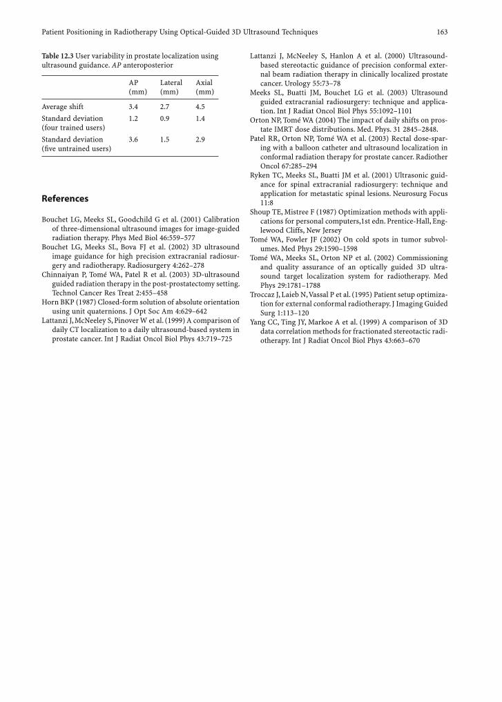
Patient Positioning in Radiotherapy Using Optical-Guided 3D Ultrasound Techniques 163

Table 12.3 User variability in prostate localization using ultrasound guidance. AP anteroposterior

AP (mm)

Lateral (mm)

Axial (mm)

Average shift 3.4 2.7 4.5

Standard deviation (four trained users)

1.2 0.9 1.4

Standard deviation (fi ve untrained users)

3.6 1.5 2.9

References

Bouchet LG, Meeks SL, Goodchild G et al. (2001) Calibration of three-dimensional ultrasound images for image-guided radiation therapy. Phys Med Biol 46:559–577

Bouchet LG, Meeks SL, Bova FJ et al. (2002) 3D ultrasound image guidance for high precision extracranial radiosur-gery and radiotherapy. Radiosurgery 4:262–278

Chinnaiyan P, Tomé WA, Patel R et al. (2003) 3D-ultrasound guided radiation therapy in the post-prostatectomy setting. Technol Cancer Res Treat 2:455–458

Horn BKP (1987) Closed-form solution of absolute orientation using unit quaternions. J Opt Soc Am 4:629–642

Lattanzi J, McNeeley S, Pinover W et al. (1999) A comparison of daily CT localization to a daily ultrasound-based system in prostate cancer. Int J Radiat Oncol Biol Phys 43:719–725

Lattanzi J, McNeeley S, Hanlon A et al. (2000) Ultrasound-based stereotactic guidance of precision conformal exter-nal beam radiation therapy in clinically localized prostate cancer. Urology 55:73–78

Meeks SL, Buatti JM, Bouchet LG et al. (2003) Ultrasound guided extracranial radiosurgery: technique and applica-tion. Int J Radiat Oncol Biol Phys 55:1092–1101

Orton NP, Tomé WA (2004) The impact of daily shifts on pros-tate IMRT dose distributions. Med. Phys. 31 2845–2848.

Patel RR, Orton NP, Tomé WA et al. (2003) Rectal dose-spar-ing with a balloon catheter and ultrasound localization in conformal radiation therapy for prostate cancer. Radiother Oncol 67:285–294

Ryken TC, Meeks SL, Buatti JM et al. (2001) Ultrasonic guid-ance for spinal extracranial radiosurgery: technique and application for metastatic spinal lesions. Neurosurg Focus 11:8

Shoup TE, Mistree F (1987) Optimization methods with appli-cations for personal computers,1st edn. Prentice-Hall, Eng-lewood Cliffs, New Jersey

Tomé WA, Fowler JF (2002) On cold spots in tumor subvol-umes. Med Phys 29:1590–1598

Tomé WA, Meeks SL, Orton NP et al. (2002) Commissioning and quality assurance of an optically guided 3D ultra-sound target localization system for radiotherapy. Med Phys 29:1781–1788

Troccaz J, Laieb N, Vassal P et al. (1995) Patient setup optimiza-tion for external conformal radiotherapy. J Imaging Guided Surg 1:113–120

Yang CC, Ting JY, Markoe A et al. (1999) A comparison of 3D data correlation methods for fractionated stereotactic radi-otherapy. Int J Radiat Oncol Biol Phys 43:663–670

Defi nition of Target Volume and Organs at Risk. Biological Target Volume 165

3D Treatment Planning for Conformal Radiotherapy

Defi nition of Target Volume and Organs at Risk. Biological Target Volume 167

13 Defi nition of Target Volume and Organs at Risk. Biological Target Volume

Anca-Ligia Grosu, Lisa D. Sprague, and Michael Molls

A.-L. Grosu, MD; L.D. Sprague, PhD; M. Molls, MDDepartment of Radiation Oncology, Klinikum rechts der Isar, Technical University Munich, Ismaningerstrasse 22, 81675 Munich, Germany

13.1 Introduction

The defi nition of the target volume and of critical structures is a crucial and complex process in three-dimensional conformal radiation therapy. In a plan-ning system, based either on computed topography (CT) or magnetic resonance imaging (MRI), the ra-diation oncologist is required to outline the target volume to be irradiated, and the organs of risk to be spared, because of possible side effects. In this process, a multitude of information has to be taken

into consideration: the results of radiological and clinical investigations; tumour staging; surgical and histo-pathological reports; other additional treat-ments such as chemotherapy; immune therapy; the patient’s history; the anatomy of the region to be irra-diated; and the acceptance of the patient concerning radiation treatment. But also the technique used for irradiation, including the patient’s positioning and fi xation, are of major importance. As a consequence, the complexity of the process when defi ning the tar-get volume requires sound clinical judgement and knowledge from the radiation oncologist.

Three-dimensional conformal treatment plan-ning in radiation oncology is based on radiological imaging, CT and MRI. These investigative techniques show the anatomical structures with a high accuracy. Both CT and MRI image tumour tissue by taking ad-vantage of the differences in tissue density (or signal intensity in MRI), contrast enhancement or the abil-ity to accumulate water (oedema). But these signals are not specifi c to tumour tissue alone. They can also be observed after a trauma or surgery, or infl amma-tory or vascular disease. This can hamper diagnosis and delineation of a tumour, and represents the most important limitation of these traditional radiological investigation techniques.

Biological imaging visualises biological pathways. Positron emission tomography (PET) and single photon computed emission tomography (SPECT) are characterised by visualising a tumour using radioac-tive tracers. These tracers have a higher affi nity for tumorous tissue in comparison with normal tissue. Magnetic resonance spectroscopy (MRS) imaging provides information on the biological activity of a tumour based on the levels of cellular metabolites; therefore, the information obtained from different imaging modalities is in general complementary by nature.

This chapter discusses the standard concepts de-fi ned in the ICRU report 50 (ICRU 50 1993) and the ICRU report 62 (ICRU 62 1999). Additionally, we dis-cuss the impact of biological investigations in target volume delineation.

CONTENTS

13.1 Introduction 16713.2 Defi nition of Target Volume 16813.2.1 Gross Target Volume 16813.2.2 Clinical Target Volume 16813.2.3 Internal Target Volume 16913.2.4 Planning Target Volume 16913.2.5 Treated Volume 16913.2.6 Irradiated Volume 16913.3 Defi nition of Organs at Risk 16913.4 New Concepts in Target Volume Defi nition: Biological Target Volume 17013.4.1 Where is the Tumour Located and Where Are the (Macroscopic) Tumour Margins? 17013.4.1.1 Lung Cancer 17013.4.1.2 Head and Neck Cancer 17213.4.1.3 Prostate Cancer 17213.4.1.4 Brain Gliomas 17213.4.2 Which Relevant Biological Properties of the Tumour Could Represent an Appropriate Biological Target for Radiation Therapy? 17313.4.3 What is the Biological Tumour Response to Therapy? 17413.5 Conclusion 175 References 176

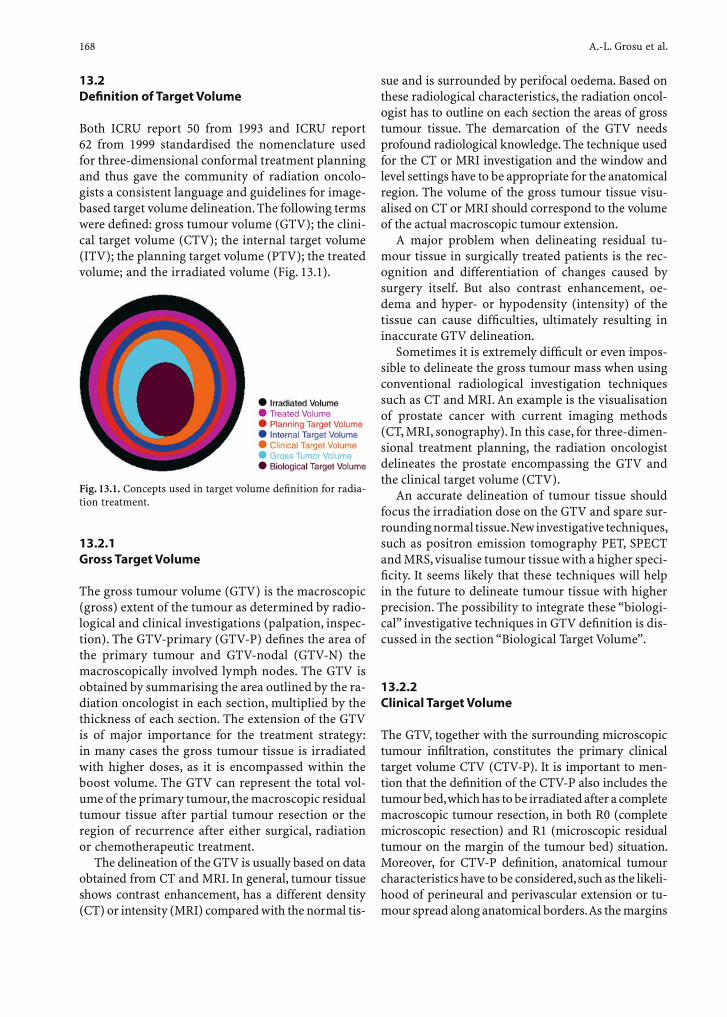
168 A.-L. Grosu et al.

13.2 Defi nition of Target Volume

Both ICRU report 50 from 1993 and ICRU report 62 from 1999 standardised the nomenclature used for three-dimensional conformal treatment planning and thus gave the community of radiation oncolo-gists a consistent language and guidelines for image-based target volume delineation. The following terms were defi ned: gross tumour volume (GTV); the clini-cal target volume (CTV); the internal target volume (ITV); the planning target volume (PTV); the treated volume; and the irradiated volume (Fig. 13.1).

sue and is surrounded by perifocal oedema. Based on these radiological characteristics, the radiation oncol-ogist has to outline on each section the areas of gross tumour tissue. The demarcation of the GTV needs profound radiological knowledge. The technique used for the CT or MRI investigation and the window and level settings have to be appropriate for the anatomical region. The volume of the gross tumour tissue visu-alised on CT or MRI should correspond to the volume of the actual macroscopic tumour extension.

A major problem when delineating residual tu-mour tissue in surgically treated patients is the rec-ognition and differentiation of changes caused by surgery itself. But also contrast enhancement, oe-dema and hyper- or hypodensity (intensity) of the tissue can cause diffi culties, ultimately resulting in inaccurate GTV delineation.

Sometimes it is extremely diffi cult or even impos-sible to delineate the gross tumour mass when using conventional radiological investigation techniques such as CT and MRI. An example is the visualisation of prostate cancer with current imaging methods (CT, MRI, sonography). In this case, for three-dimen-sional treatment planning, the radiation oncologist delineates the prostate encompassing the GTV and the clinical target volume (CTV).

An accurate delineation of tumour tissue should focus the irradiation dose on the GTV and spare sur-rounding normal tissue. New investigative techniques, such as positron emission tomography PET, SPECT and MRS, visualise tumour tissue with a higher speci-fi city. It seems likely that these techniques will help in the future to delineate tumour tissue with higher precision. The possibility to integrate these “biologi-cal” investigative techniques in GTV defi nition is dis-cussed in the section “Biological Target Volume”.

13.2.2 Clinical Target Volume

The GTV, together with the surrounding microscopic tumour infi ltration, constitutes the primary clinical target volume CTV (CTV-P). It is important to men-tion that the defi nition of the CTV-P also includes the tumour bed, which has to be irradiated after a complete macroscopic tumour resection, in both R0 (complete microscopic resection) and R1 (microscopic residual tumour on the margin of the tumour bed) situation. Moreover, for CTV-P defi nition, anatomical tumour characteristics have to be considered, such as the likeli-hood of perineural and perivascular extension or tu-mour spread along anatomical borders. As the margins

Fig. 13.1. Concepts used in target volume defi nition for radia-tion treatment.

13.2.1 Gross Target Volume

The gross tumour volume (GTV) is the macroscopic (gross) extent of the tumour as determined by radio-logical and clinical investigations (palpation, inspec-tion). The GTV-primary (GTV-P) defi nes the area of the primary tumour and GTV-nodal (GTV-N) the macroscopically involved lymph nodes. The GTV is obtained by summarising the area outlined by the ra-diation oncologist in each section, multiplied by the thickness of each section. The extension of the GTV is of major importance for the treatment strategy: in many cases the gross tumour tissue is irradiated with higher doses, as it is encompassed within the boost volume. The GTV can represent the total vol-ume of the primary tumour, the macroscopic residual tumour tissue after partial tumour resection or the region of recurrence after either surgical, radiation or chemotherapeutic treatment.

The delineation of the GTV is usually based on data obtained from CT and MRI. In general, tumour tissue shows contrast enhancement, has a different density (CT) or intensity (MRI) compared with the normal tis-

Defi nition of Target Volume and Organs at Risk. Biological Target Volume 169

between CTV and GTV are not homogenous, they have to be adjusted to the probable microscopic tumour spread. The CTV-nodal (CTV-N) defi nes the assumed microscopic lymphatic tumour spread, which has also to be included in the radiation treatment planning.

13.2.3 Internal Target Volume

The internal target volume (ITV) is a term intro-duced by the ICRU report 62. The ITV encompasses the GTV/CTV plus internal margins to the GTV/CTV, caused by possible physiological movements of or-gans and tumour, due to respiration, pulsation, fi ll-ing of the rectum, or variations of tumour size and shape, etc. It is defi ned in relation to internal ref-erence points, most often rigid bone structures, in an internal patient coordinate system. Observation of internal margins is diffi cult, in many cases even impossible. Examples for reducing internal margins are the fi xation of the rectum with a balloon during irradiation of the prostate or body fi xation and ad-ministration of oxygen to reduce respiration move-ments during stereotactic radiotherapy.

13.2.4 Planning Target Volume

The planning target volume (PTV) incorporates the GTV/CTV plus margins due to uncertainties of pa-tient setup and beam adjustment; therefore, these margins consider the inaccuracy in the geometrical location of the GTV/CTV in the irradiated space, due to variations in patient positioning during radiother-apy and organ motility. The PTV can be compared with an envelope and has to be treated with the same irradiation dose as the GTV/CTV. Movements of the GTV/CTV within this envelope should not change the delivered radiation dose to the GTC and CTV. The setup margins are not uniform. The radiation oncologist should defi ne the margins together with the radiation physicist, taking into consideration the possible inaccuracy in patient and beam positioning. Signifi cant reduction of setup margins can be ob-tained by applying patient fi xation and re-position-ing techniques, as used, for example, in stereotactic radiotherapy. Beam positioning uncertainties should be subject of a specifi c quality control program of each treatment unit. Consequently, the volume of normal tissue surrounding the tumour and included in high irradiation dose areas can be considerably

reduced and the dose applied to the GTV/CTV can be escalated.

13.2.5 Treated Volume

The treated volume is the volume of tumour and surrounding normal tissue included in an isodose surface representing the irradiation dose proposed for the treatment. As a rule this corresponds to the 95% isodose. Ideally, the treated volume should cor-respond to the PTV; however, in many cases the treated volume exceeds the PTV. The coherence of an irradiation plan can be described/illustrated as the correlation between PTV and treated volume.

13.2.6 Irradiated Volume

The irradiated volume is a volume included in an isodose surface with a possible biological impact on the normal tissue encompassed in this volume; there-fore, the irradiated volume depends on the selected isodose curve and the normal tissue surrounding the tumour. The choice of an isodose surface depends on the end point defi ned for possible side effects in normal tissue. For grade-III and grade-IV side ef-fects, the isodoses will correspond to higher doses, whereas low-dose areas are signifi cant for the risk of carcinogenesis.

13.3 Defi nition of Organs at Risk

Organs at risk (ICRU report 50), also known as criti-cal structures, are anatomical structures with impor-tant functional properties located in the vicinity of the target volume. They have to be considered in the treatment planning, since irradiation can cause pathological changes in normal tissue, with irrevers-ible functional consequences. The critical structures must be outlined in the planning process and the dose applied to these areas has to be quantifi ed by ei-ther visualising the isodose distribution or by means of dose-volume histograms (DVH). It is essential to include the tolerance dose of the organs at risk in the treatment strategy.

The ICRU report 62 furthermore added the term “planning organs at risk volume” (PRV). This term

170 A.-L. Grosu et al.

takes into account that the organs at risk are in the majority mobile structures; therefore, a surrounding margin is added to the organs at risk in order to com-pensate for geometric uncertainties.

With regard to histopathological properties of tissue, organs at risk can be classifi ed as serial, parallel and serial-parallel (Källmann et al. 1992; Jackson and Kutcher 1993). Serial organs can lose their complete functionality even if only a small volume of the organ receives a dose above the tolerance limit. Best known ex-amples are spinal cord, optical nerve and optical chiasm. In contrast, parallel organs are damaged only if a larger volume is included in the irradiation region, e.g. lung and kidney; however, in many cases these two models are combined in a serial-parallel organ confi guration. Side effects occur due to various pathological mecha-nisms, size of the irradiated volume and the maximal dose applied to the organ. A classical example for a se-rial-parallel organ is the heart: the coronary arteries are a parallel and the myocardium a serial organ.

The organs at risk can be located at a distance from the PTV, close to the PTV or incorporated within the tumour tissue and thus be in the PTV. These three situations have to be considered in the treatment planning. Organs with a low tolerance to irradiation (lens, gonads) have to be outlined even if they are not located in the immediate vicinity of the PTV. For or-gans situated close to the PTV a plan with a very deep dose fall towards the critical structures has to be de-signed. If the organs at risk are encompassed within the PTV, it is crucial to achieve a homogeneous dose distribution, and to consider the Dmax and the iso-dose distribution in the PTV.

13.4 New Concepts in Target Volume Defi nition: Biological Target Volume

In recent years, new methods for tumour visualisation have begun to have a major impact on radiation oncol-ogy. Techniques such as PET, SPECT and MRS permit the visualisation of molecular biological pathways in tumours; thus, additional information about metabo-lism, physiology and molecular biology of tumour tis-sue can be obtained. This new class of images, showing specifi c biological events, seems to complement the anatomical information from traditional radiological investigations. Accordingly, in addition to the terms GTV, CTV, PTV, etc., LING et al. (2000) proposed the terms “biological target volume” (BTV) and “multidi-mensional conformal radiotherapy” (MD-CRT).

Thus far, biological imaging has not yet been in-tegrated into radiation treatment planning; however, several trials indicate that biological imaging could have a signifi cant impact on the development of new treatment strategies in radiation oncology. These tri-als show that PET, SPECT or MRS might be helpful in obtaining more specifi c answers to the three essential questions given in the sections that follow.

13.4.1 Where is the Tumour Located and Where Are the (Macroscopic) Tumour Margins?

The co-registration of biological and anatomical im-aging techniques seems to improve the delineation of viable tumour tissue compared with CT or MRI alone. Biological imaging enables the defi nition of a target volume on the basis of biological processes. For some cases this results in clearer differentiation between tumour and normal tissue as compared with CT and MRI alone; however, anatomical imag-ing will continue to be the basis of treatment plan-ning because of its higher resolution. Incorporation of biological imaging into the tumour volume defi ni-tion should only be done in tumours with increased sensitivity and specifi city to biological investigation techniques.

We discuss three clinical entities: lung cancer, head and neck cancer, prostate cancer and brain gliomas as biological imaging proved to be helpful in target volume delineation.

13.4.1.1 Lung Cancer

The role of fl uoro-deoxyglucose (FDG)-PET in ra-diation treatment planning of lung cancer has been thoroughly investigated in a total of 415 patients in 11 trials (Table 13.1; Grosu et al. 2005c). These inves-tigations compared FDG-PET data with CT data. The CT/PET image fusion methods were used in fi ve tri-als. One study used the integrated PET/CT system. All these studies suggested that FDG-PET adds essential information to the CT with signifi cant consequences on GTV, CTV and PTV defi nition. The percentage of cases presenting signifi cant changes in tumour volume after the integration of FDG-PET investigation in the radiation treatment planning ranged from 21 to 100%. Ten studies pointed out the signifi cant implications of FDG-PET in staging lymph node involvement. These fi ndings are supported by data in the literature, show-ing an advantage of FDG-PET over CT in lung cancer

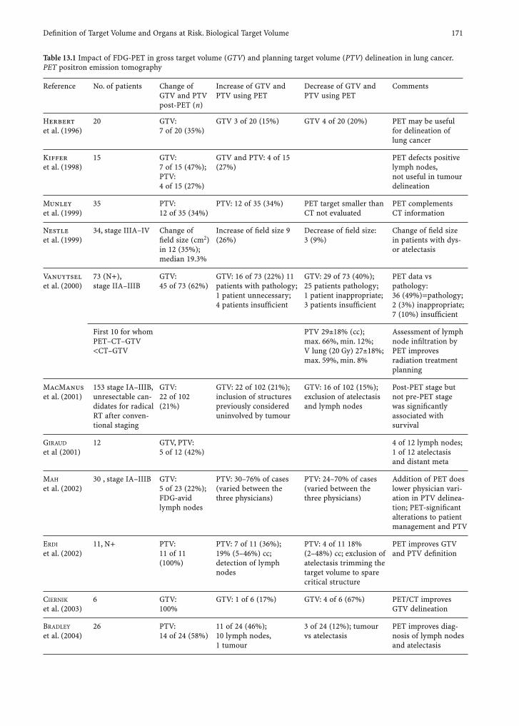
Defi nition of Target Volume and Organs at Risk. Biological Target Volume 171

Table 13.1 Impact of FDG-PET in gross target volume (GTV) and planning target volume (PTV) delineation in lung cancer. PET positron emission tomography

Reference No. of patients Change of GTV and PTV post-PET (n)

Increase of GTV and PTV using PET

Decrease of GTV and PTV using PET

Comments

Herbert et al. (1996)

20 GTV: 7 of 20 (35%)

GTV 3 of 20 (15%) GTV 4 of 20 (20%) PET may be useful for delineation of lung cancer

Kiffer et al. (1998)

15 GTV: 7 of 15 (47%); PTV: 4 of 15 (27%)

GTV and PTV: 4 of 15 (27%)

PET defects positive lymph nodes, not useful in tumour delineation

Munley et al. (1999)

35 PTV: 12 of 35 (34%)

PTV: 12 of 35 (34%) PET target smaller than CT not evaluated

PET complements CT information

Nestle et al. (1999)

34, stage IIIA–IV Change of fi eld size (cm2) in 12 (35%); median 19.3%

Increase of fi eld size 9 (26%)

Decrease of fi eld size: 3 (9%)

Change of fi eld size in patients with dys- or atelectasis

Vanuytsel et al. (2000)

73 (N+), stage IIA–IIIB

GTV: 45 of 73 (62%)

GTV: 16 of 73 (22%) 11 patients with pathology; 1 patient unnecessary; 4 patients insuffi cient

GTV: 29 of 73 (40%); 25 patients pathology; 1 patient inappropriate; 3 patients insuffi cient

PET data vs pathology: 36 (49%)=pathology; 2 (3%) inappropriate; 7 (10%) insuffi cient

First 10 for whom PET–CT–GTV<CT–GTV

PTV 29±18% (cc); max. 66%, min. 12%; V lung (20 Gy) 27±18%; max. 59%, min. 8%

Assessment of lymph node infi ltration by PET improves radiation treatment planning

MacManus et al. (2001)

153 stage IA–IIIB, unresectable can-didates for radical RT after conven-tional staging

GTV: 22 of 102 (21%)

GTV: 22 of 102 (21%); inclusion of structures previously considered uninvolved by tumour

GTV: 16 of 102 (15%); exclusion of atelectasis and lymph nodes

Post-PET stage but not pre-PET stage was signifi cantly associated with survival

GIRAUD et al (2001)

12 GTV, PTV: 5 of 12 (42%)

4 of 12 lymph nodes; 1 of 12 atelectasis and distant meta

MAH et al. (2002)

30 , stage IA–IIIB GTV: 5 of 23 (22%); FDG-avid lymph nodes

PTV: 30–76% of cases (varied between the three physicians)

PTV: 24–70% of cases (varied between the three physicians)

Addition of PET does lower physician vari-ation in PTV delinea-tion; PET-signifi cant alterations to patient management and PTV

ERDI et al. (2002)

11, N+ PTV: 11 of 11 (100%)

PTV: 7 of 11 (36%); 19% (5–46%) cc; detection of lymph nodes

PTV: 4 of 11 18% (2–48%) cc; exclusion of atelectasis trimming the target volume to spare critical structure

PET improves GTV and PTV defi nition

CIERNIK et al. (2003)

6 GTV: 100%

GTV: 1 of 6 (17%) GTV: 4 of 6 (67%) PET/CT improves GTV delineation

BRADLEY et al. (2004)

26 PTV: 14 of 24 (58%)

11 of 24 (46%); 10 lymph nodes, 1 tumour

3 of 24 (12%); tumour vs atelectasis

PET improves diag-nosis of lymph nodes and atelectasis

172 A.-L. Grosu et al.

staging. The PET may help to differentiate between vi-able tumour tissue and associated atelectasis; however, it shows limitations when secondary infl ammation is present. As GTV delineation is a fundamental step in radiation treatment planning, the use of combined CT/PET imaging for all dose escalation studies with either conformal radiotherapy or IMRT has been rec-ommended by RTOG as a standard method in lung cancer (Chapman et al. 2003).

13.4.1.2 Head and Neck Cancer

A signifi cant number of studies have demonstrated that FDG-PET can be superior to CT and MRI in the detection of lymph nodes metastases, the identifi ca-tion of unknown primary cancer and in the detection of viable tumour tissue after treatment.

Rahn et al. (1998) studied 34 patients with histolog-ically confi rmed squamous cell carcinoma of the head and neck by performing FDG-PET prior to treatment planning in addition to conventional staging proce-dures, including CT, MRI and ultrasound. The integra-tion of FDG-PET in radiation treatment planning led to signifi cant changes in the radiation fi eld and dose in 9 of 22 (44%) patients with a primary tumour and in 7 of 12 (58%) patients with tumour recurrence. This was due mainly to the inclusion of lymph nodes metastases detected by FDG-PET. In a recent study, Nishioka et al. (2002) showed that the integration of FDG-PET in radiation treatment planning might also cause a reduc-tion in the size of the radiation fi elds. The GTV for pri-mary tumour was not altered by image fusion in 19 of 21 (90%) patients. Of the 9 patients with nasopharynx cancer, the GTV was enlarged by 49% in only 1 patient and decreased by 45% in 1 patient. In 15 of 21 (71%) patients the tumour-free FDG-PET detection allowed normal tissue to be spared. Mainly, parotid glands were spared and, thus, xerostomia was avoided. The authors concluded that the image fusion between FDG-PET and MRI/CT was useful in GTV, CTV and PTV determina-tion, both for encompassing the whole tumour area in the irradiation fi eld and for sparing of normal tissue. The integrated PET/CT was used for GTV and PTV def-inition in 12 patients with head and neck tumours and compared with CT alone. The GTV increased by 25% or more due to FDG-PET in 17% of these cases and was reduced by 25 in 33% of the patients. The correspond-ing change in PTV was approximately 20%; however, this study did not integrate MRI in the analysis, which has a higher sensitivity than CT (Ciernik et al. 2003).

In conclusion, the value of FDG-PET for radiation treatment planning is still under investigation. In

some cases, FDG-PET visualised tumour infi ltration better than CT or MRI alone. The FDG-PET could also play an important role in the defi nition of the boost volume for radiation therapy; however, the rel-atively high FDG uptake in infl ammation areas could sometimes lead to false-positive results.

13.4.1.3 Prostate Cancer

Choline and citrate metabolism within cytosol and the extracellular space were investigated in prostate cancer using H-MRS. Clinical trials analysing tumour location and extent within the prostate, extra-capsu-lar spread and cancer aggressiveness in pre-prosta-tectomy patients have indicated that the metabolic information provided by H-MRS combined with the anatomical information provided by MRI can sig-nifi cantly improve the tumour diagnosis and the outline of tumour extension (Mizowaki et al. 2002; Mueller-Lisse et al. 2001; Wefer et al. 2000).

Coakley et al. (2002) evaluated endorectal MRI and 3D MRS in 37 patients before prostatectomy and correlated the tumour volumes measured with MRI and H-MRS with the true tumour volume mea-sured after prostatectomy. Measurements of tumour volume with MRI, MRS and a combination of both were all positively correlated with histopathological volume (Pearson’s correlation coeffi cient of 0.49, 0.59 and 0.55, respectively), but only measurements with 3D MRS and a combination of MRI and MRS were statistically signifi cant (p<0.05).

The integration of H-MRS in brachytherapy treat-ment planning for target volume defi nition in pa-tients with organ-confi ned but aggressive prostatic cancer could improve the tumour control probability (Zaider et al. 2000).

13.4.1.4 Brain Gliomas

Although only preliminary data are available, the presented literature indicates that amino-acid PET, SPECT and H-MRS, in addition to conventional mor-phological imaging, are superior to the exclusive use of either MRI or CT in the visualisation of vital tu-mour extension in gliomas (Table 13.2).

Our group investigated the value of amino-acid PET and SPECT in GTV, PTV and boost volume (BV) defi nition for radiation treatment planning of brain gliomas. We demonstrated that I-123-alpha-methyl-tyrosine (IMT)-SPECT and L-(methyl-11C) methio-nine (MET)-PET offer signifi cant additional infor-

Defi nition of Target Volume and Organs at Risk. Biological Target Volume 173

mation concerning tumour extension in high-grade gliomas, compared with anatomical imaging (CT and MRI) alone (Grosu et al. 2000, 2002, 2003, 2005a,c). The MRS studies led to similar results (Pirzkall et al. 2001, 2004). A current analysis of an amino-acid SPECT- or PET-planned subgroup of patients with recurrent gliomas suggests that the integration of amino-acid PET or SPECT in target volume defi nition might contribute to an improved outcome (Fig. 13.2; Grosu et al. 2005b).

13.4.2 Which Relevant Biological Properties of the Tumour Could Represent an Appropriate Biological Target for Radiation Therapy?

Tumour hypoxia (Fig. 13.3) is an unfavourable prog-nostic indicator in cancer as it can be linked to ag-gressive growth, metastasis and poor response to treatment (Molls and Vaupel 2000; Molls 2001). In a clinical pilot study, Chao et al. (2001) demon-strated the feasibility of [60Cu]ATSM-PET guided radiotherapy planning in head and neck cancer pa-tients; however, the tumour-to-background ratio in hypoxic tumour tissues did not dramatically differ from previous studies using [18F]FMISO and other nitroimidazole compounds. The authors reported the integration of the hypoxia tracer Cu-ATSM in radia-tion treatment planning for patients with locally ad-vanced head and neck cancer treated with IMRT. They developed a CT/PET fusion image based on external markers. The GTV outline was based on radiological and PET fi ndings. Within the GTV, regions with a Cu-ATSM uptake twice that of the contralateral normal neck muscle were selected and outlined as hypoxic

GTV (hGTV). The IMRT plan delivered 80 Gy in 35 fractions to the ATSM-enriched tumour subvolume (hGTV) and the GTV received simultaneously 70 Gy in 35 fractions, keeping the radiation dose to the pa-rotid glands below 30 Gy.

More recently, Dehdashti et al. (2003) were the fi rst to demonstrate a negative predictive value of en-hanced Cu-ATSM uptake for the response to treatment in 14 cervical cancer patients. Rischin et al. (2001) used 18F-misonidazole scans to detect hypoxia in pa-tients with T3/4, N2/3 head and neck tumours treated with tirapazamine, cisplatin and radiation therapy. Fourteen of 15 patients were hypoxia positive at the beginning of the treatment, but only one patient had detectable hypoxia at the end of radiochemotherapy.

By imaging either hypoxia (Rischin et al. 2001) with 18F-misonidazole or [60Cu]ATSM (Chao et al. 2001), angiogenesis with 18F-labelled RDG-contain-ing glycopeptide and PET (Haubner et al. 2001), proliferation with fl uorine-labelled thymidine ana-logue 3’-deoxy-3’-[18F]-fl uorothymidine (FLT) and PET (Wagner et al. 2003), or apoptosis with a ra-dio-labelled recombinant Annexin V and SPECT (Belhocine et al. 2004), different areas within a tu-mour can be identifi ed and individually targeted. This approach, closely related to the IMRT technique, has been named “dose painting”. The IMRT combined with a treatment plan based on biological imaging could be used for individualised, i.e. customised, ra-diation therapy. The biological process visualised by the tracer needs to be specifi ed; therefore, the selected BTV should be named after the respective tracer (i.e. BTV(FDG-PET), BTV(FAZA-PET); Grosu et al. 2005c).

This novel treatment approach will generate a new set of problems and questions such as: What are the dynamics of the visualised biological processes? How

Table 13.2 Impact of biological imaging: PET, SPECT and MRS in target volume delineation of gliomas. High G high-grade gliomas

Reference No. of patients Diagnosis Biological imaging Additional information to MRI and CT

Voges (1997) 46 Low+high G MET-PET, FDG-PET Yes

Julow (2000) 13 High G MET-PET, SPECT ? Yes

Gross (1998) 18 High G FDG-PET No

Nuutinen (2000) 11 Low G MET-PET Yes

Grosu (2000) 30 Low+high G IMT-SPECT Yes

Graves (2000) 36 High G H-MRS Yes

Pirzkall (2001) 40 High G H-MRS Yes

Pirzkall (2004) 30 High G H-MRS Yes

Grosu (2002) 66 High G IMT-SPECT Yes

Grosu (2005) 44 High G MET-PET Yes

174 A.-L. Grosu et al.

many biological investigations are necessary dur-ing treatment and when? Which radiation treatment schedules have to be applied?

Prospective clinical trials and experimental stud-ies should supply the answers to these questions.

13.4.3 What is the Biological Tumour Response to Therapy?

Biological imaging could be used to evaluate the re-sponse of a tumour to different therapeutic interven-tions. The usefulness of PET for monitoring patients treated with chemotherapy has been documented in several studies. Although evaluating the response af-

Fig. 13.2. MET-PET data were integrated in the planning system and were co-registered with the CT and MRI data using an automatically, intensity based image fusion method – Brain LAB (Grosu et al. 2005b)

ter radiochemotherapy is often diffi cult due to treat-ment-induced infl ammatory tissue changes, prelimi-nary data for lung (Weber et al. 2003; MacManus et al. 2003; Choi 2002), oesophageal (Flamen et al. 2002) and cervical cancer (Grigsby et al. 2003) sug-gest that the decrease of FDG uptake after treatment correlates with histological tumour remission and longer survival; however, it still has to be clarifi ed at which time points PET imaging should be performed, which tracer is to be used and which criteria can be used for the defi nition of a tumour response in PET. Theoretically, the integration of biological imaging in treatment monitoring could have signifi cant conse-quences for future radiation treatment planning. This could result in changes of target volume/boost vol-

Defi nition of Target Volume and Organs at Risk. Biological Target Volume 175

radiation oncologist has to outline the GTV, CTV, ITV and PTV and BTV. In this process, a lot of medical and technological aspects have to be considered. The criteria for GTV, CTV, etc. defi nition are often not exactly standardised, and this leads, in many cases, to variability between clinicians; however, exactly de-fi ned imaging criteria, imaging with high sensitivity and specifi city for tumour tissue and special training could lead to a higher consensus in target volume delineation and, consequently, to lower differences between clinicians. It must be emphasised, however, that further verifi cation studies and cost-benefi t analyses are needed before biological target defi ni-tion can become a stably integrated part of target volume defi nition.

The ICRU report 50 from 1993 and the ICRU re-port 62 from 1999 defi ning the anatomically based terms CTV, GTV and PTV must still be considered as the gold standard in radiation treatment planning; however, further advances in technology concerning

ume delineation during radiation therapy; however, this still has to be analysed in clinical studies.

In summary, biological imaging allows the visu-alisation of fundamental biological processes in ma-lignancies. To date, the suggested superiority of bio-logical strategies for treatment planning has not yet been suffi ciently demonstrated; therefore, before the BTV defi nition can be generally recommended, fur-ther clinical studies based on integrated PET, SPECT or MRS need to be conducted. These studies must compare the outcome of biologically based treatment regimes with conventional treatment regimes.

13.5 Conclusion

Target volume defi nition is an interactive process. Based on radiological (and biological) imaging, the

Fig. 13.3. Imaging of hypoxia in a patient with a cT4 cN2 cM0 G2 laryngeal cancer. [18F]Azomycin arabinoside [18F]FAZA-PET/CT image fusion. Using IMRT the hypoxic area is encompassed in the high dose area (BTV, orange) and the CTV is encompassed in the lower dose area - green. (Courtesy of Dr. M. Piert, Nuclear Medicine Department, Technical University Munich, Germany)

176 A.-L. Grosu et al.

signal resolution and development of new tracers with higher sensitivity and specifi city will induce a shift of paradigms away from the anatomically based target volume defi nition towards biologically based treatment strategies. New concepts and treatment strategies should be defi ned based on these new in-vestigation methods, and the standards in radiation treatment planning – in a continuous, evolutionary process – will have to integrate new imaging methods in an attempt to fi nally achieve the ultimate goal of cancer cure.

References

Belhocine T, Steinmetz N, Li C et al. (2004) The imaging of apoptosis with the radiolabeled annexin V: optimal timing for clinical feasibility. Technol Cancer Res Treat 3:23–32

Bradley J, Thorstad WL, Mutic S et al. (2004) Impact of FDG–PET on radiation therapy volume delineation in NSCLC. Int J Radiat Oncol Biol Phys 59:78–86

Chao KS, Bosch WR, Mutic S et al. (2001) A novel approach to overcome hypoxic tumour resistance: Cu-ATSM-guided intensity-modulated radiation therapy. Int J Radiat Oncol Biol Phys 49:1171–1182

Chapman JD, Bradley JD, Eary JF et al. (2003) Molecular (func-tional) imaging for radiotherapy applications: an RTOG symposium. Int J Radiat Oncol Biol Phys 55:294–301

Choi NC, Fischman AJ, Niemierko A et al. (2002) Dose-response relationship between probability of pathologic tumour control and glucose metabolic rate measured with FDG PET after preoperative chemoradiotherapy in locally advanced non-small-cell lung cancer. Int J Radiat Oncol Biol Phys 54:1024–1035

Ciernik IF, Dizendorf E, Baumert BG et al. (2003) Radiation treatment planning with an integrated positron emission and computer tomography (PET/CT): a feasibility study. Int J Radiat Oncol Biol Phys 57:853–863

Coakley FV, Kurhanewicz J, Lu Y et al. (2002) Prostate cancer tumour volume: measurement with endorectal MR and MR spectroscopic imaging. Radiology 223:91–97

Dehdashti F, Grigsby PW, Mintun MA et al. (2003) Assessing tumour hypoxia in cervical cancer by positron emission tomography with 60Cu-ATSM: relationship to therapeutic response: a preliminary report. Int J Radiat Oncol Biol Phys 55:1233–1238

Erdi YE, Rosenzweig K, Erdi AK et al. (2002) Radiotherapy treatment planning for patients with non-small cell lung cancer using positron emission tomography (PET). Radio-ther Oncol 62:51–60

Flamen P, Van Cutsem E, Lerut A et al. (2002) Positron emis-sion tomography for assessment of the response to induc-tion radiochemotherapy in locally advanced oesophageal cancer. Ann Oncol 13:361–368

Giraud P, Grahek D, Montravers F et al. (2001) CT and (18)F-deoxyglucose (FDG) image fusion for optimization of con-formal radiotherapy of lung cancers. Int J Radiat Oncol Biol Phys 49:1249–1257

Graves EE, Nelson SJ, Vigneron DB et al. (2000) A preliminary study of the prognostic value of proton magnetic reso-nance spectroscopic imaging in gamma knife radiosurgery of recurrent malignant gliomas. Neurosurgery 46:319–326

Grigsby PW, Siegel BA, Dehdashti F et al. (2003) Posttherapy surveillance monitoring of cervical cancer by FDG–PET. Int J Radiat Oncol Biol Phys 55:907–913

Gross MW, Weber WA, Feldmann HJ et al. (1998) The value of F-18-fl uorodeoxyglucose PET for the 3-D radiation treat-ment planning of malignant gliomas. Int J Radiat Oncol Biol Phys 41:989–995

Grosu AL, Weber WA, Feldmann HJ et al. (2000) First experi-ence with I-123-Alpha-Methyl-Tyrosine SPECT in the 3-D radiation treatment planning of brain gliomas. Int J Radiat Oncol Biol Phys 47:517–527

Grosu AL, Feldmann HJ, Dick S et al. (2002) Implications of IMT-SPECT for postoperative radiation treatment plan-ning in patients with gliomas. Int J Radiat Oncol Biol Phys 54:842–854

Grosu AL, Lachner R, Wiedenmann N et al. (2003) Validation of a method for automatic fusion of CT- and C11-methio-nine-PET datasets of the brain for stereotactic radiother-apy using a LINAC. First clinical experience. Int J Radiat Oncol Biol Phys 56:1450–1463

Grosu AL, Weber AW, Riedel E et al. (2005a) L-(Methyl-11C) methionine positron emission tomography for target delineation in resected high grade gliomas before radia-tion therapy. Int J Radiat Oncol Biol Phys 63:64–74

Grosu AL, Weber WA, Franz M et al. (2005b) Re-irradiation of recurrent high grade gliomas using amino-acids–PET(SPECT)/CT/MRI image fusion to determine gross tumour volume for stereotactic fractionated radiotherapy. Int J Radiat Oncol Biol Phys (in press)

Grosu AL, Piert M, Weber WA et al. (2005c) Positron emission tomography in target volume defi nition for radiation treat-ment planning. Strahlenther Onkol 181:483–499

Haubner R, Wester HJ, Weber WA et al. (2001) Noninvasive imaging of alpha(v)beta3 integrin expression using 18F-labeled RGD-containing glycopeptide and positron emis-sion tomography. Cancer Res 61:1781–1785

Hebert ME, Lowe VJ, Hoffman JM et al. (1996) Positron emis-sion tomography in the pretreatment evaluation and follow-up of non-small cell lung cancer patients treated with radiotherapy: preliminary fi ndings. Am J Clin Oncol 19:416–421

ICRU 50 (1993) Prescribing, recording and reporting photon beam therapy. ICRU report no. 50. ICRU, Bethesda, Mary-land

ICRU 62 (1999) Prescribing, recording and reporting photon beam therapy. ICRU report no. 62 (supplement to ICRU report no. 50). ICRU, Bethesda, Maryland

Jackson A, Kutcher GJ (1993) Probability of radiation-induced complications for normal tissue with parallel architecture subject to non-uniform irradiation. Med Phys 20:621–625

Julow J, Major T, Emri M et al. (2000) The application of image fusion in stereotactic brachytherapy of brain tumours. Acta Neurochir (Wien) 142:1253–1258

Källmann P, Ägren A, Brahme A (1992) Tumour and normal tissue responses to fractionated nonuniform dose delivery. Int J Radiat Oncol Biol Phys 62:249–262

Kiffer JD, Berlangieri SU, Scott AM et al. (1998) The contri-bution of 18F-fl uoro–2-deoxy-glucose positron emission

Defi nition of Target Volume and Organs at Risk. Biological Target Volume 177

tomographic imaging to radiotherapy planning in lung cancer. Lung Cancer 19:167–177

Ling CC, Humm J, Larson S et al. (2000) Towards multidi-mensional radiotherapy (MD-CRT): biological imaging and biological conformality. Int J Radiat Oncol Biol Phys 47:551–560

MacManus MP, Hicks RJ, Ball DL et al. (2001) F-18 fl uorode-oxyglucose positron emission tomography staging in radi-cal radiotherapy candidates with nonsmall cell lung carci-noma: powerful correlation with survival and high impact on treatment. Cancer 92:886–895

MacManus MP, Hicks RJ, Matthews JP et al. (2003) Positron emission tomography is superior to computed tomography scanning for response assessment after radical radiother-apy or chemoradiotherapy in patients with non-small-cell lung cancer. J Clin Oncol 21:1285–1292

Mah K, Caldwell CB, Ung YC et al. (2002) The impact of (18)FDG–PET on target and critical organs in CT-based treatment planning of patients with poorly defi ned non-small-cell lung carcinoma: a prospective study. Int J Radiat Oncol Biol Phys 52:339–350

Mizowaki T, Cohen GN, Fung AY et al. (2002) Towards integrat-ing functional imaging in the treatment of prostate cancer with radiation: the registration of the MR spectroscopy imaging to ultrasound/CT images and its implementa-tion in treatment planning. Int J Radiat Oncol Biol Phys 54:1558–1564

Molls M (2001) Tumor oxygenation and treatment outcome. In: Bokemeyer C, Ludwig H (eds) ESO scientifi c updates, vol 6: Anemia in cancer. Elsevier, Amsterdam, pp 175–187

Molls M, Vaupel P (2000) The impact of the tumor environ-ment on experimental and clinical radiation oncology and other therapeutic modalities. In: Molls M, Vaupel P (eds) Blood perfusion and microenvironment of human tumors: implications for clinical radiooncology. Springer, Berlin Heidelberg New York, pp 1–3

Mueller-Lisse UG, Vigneron DB, Hricak H et al. (2001) Local-ized prostate cancer: effect of hormone deprivation therapy measured by using combined three-dimensional 1H MR spectroscopy and MR imaging: clinicopathologic case-con-trolled study. Radiology 221:380–390

Munley MT, Marks LB, Scarfone C et al. (1999) Multimodality nuclear medicine imaging in three-dimensional radiation treatment planning for lung cancer: challenges and pros-pects. Lung Cancer 23:105–114

Nestle U et al. (1999) 18F-deoxyglucose positron emission tomography (FDG-PET) for the planning of radiotherapy in lung cancer: high impact in patients with atelectasis. Int J Radiat Oncol Biol Phys 44(3):593-7.

Nishioka T, Shiga T, Shirato H et al. (2002) Image fusion between 18FDG-PET and MRI/CT for radiotherapy plan-ning of oropharyngeal and nasopharyngeal carcinomas. Int J Radiat Oncol Biol Phys 53:1051–1057

Nuutinen J, Sonninen P, Lehikoinen P et al. (2000) Radio-therapy treatment planning and long-term follow-up with [(11)C]methionine PET in patients with low-grade astro-cytoma. Int J Radiat Oncol Biol Phys 48:43–52

Pirzkall A, McKnight TR, Graves EE et al. (2001) MR-spectros-copy guided target delineation for high-grade gliomas. Int J Radiat Oncol Biol Phys 50:915–928

Pirzkall A, Li X, Oh J et al. (2004) 3D MRSI for resected high-grade gliomas before RT: tumour extent according to meta-bolic activity in relation to MRI. Int J Radiat Oncol Biol Phys 59:126–137

Rahn AN, Baum RP, Adamietz IA et al. (1998) Value of 18F fl uorodeoxyglucose positron emission tomography in radiotherapy planning of head–neck tumours. Strahlen-ther Onkol 174:358–364 [in German]

Rischin D, Peters L, Hicks R et al. (2001) Phase I trial of concurrent tirapazamine, cisplatin, and radiotherapy in patients with advanced head and neck cancer. J Clin Oncol 19:535–542

Vanuytsel LJ, Vansteenkiste JF, Stroobants SG et al. (2000) The impact of (18)F-fl uoro-2-deoxy-D-glucose positron emis-sion tomography (FDG–PET) lymph node staging on the radiation treatment volumes in patients with non-small cell lung cancer. Radiother Oncol

Voges J, Herholz K, Holzer T et al. (1997) 11C-methionine and 18F-2-fl uorodeoxyglucose positron emission tomography: a tool for diagnosis of cerebral glioma and monitoring after brachytherapy with 125-I seeds. Stereotact Funct Neuro-surg 69:129–135

Wagner M, Seitz U, Buck A et al. (2003) 3‘-[18F]fl uoro-3‘-deoxythymidine ([18F]-FLT) as positron emission tomog-raphy tracer for imaging proliferation in a murine B-cell lymphoma model and in the human disease. Cancer Res 63:2681–2687

Weber WA, Petersen V, Schmidt B et al. (2003) Positron emis-sion tomography in non-small-cell lung cancer: prediction of response to chemotherapy by quantitative assessment of glucose use. J Clin Oncol 21:2651–2657

Wefer AE, Hricak H, Vigneron DB et al. (2000) Sextant locali-zation of prostate cancer: comparison of sextant biopsy, magnetic resonance imaging and magnetic resonance spectroscopic imaging with step section histology. J Urol 164:400–404

Zaider M, Zelefsky MJ, Lee EK et al. (2000) Treatment planning for prostate implants using magnetic-resonance spectros-copy imaging. Int J Radiat Oncol Biol Phys 47:1085–1096

Virtual Therapy Simulation 179

14 Virtual Therapy Simulation

Rolf Bendl

R. Bendl, PhDAbteilung Medizinische Physik in der Strahlentherapie, Deutsches Krebsforschungszentrum, Im Neuenheimer Feld 280, 69120 Heidelberg, Germany

14.1 Introduction

Therapy simulation is widely used and has a long tradition in radiotherapy. A therapy simulator is an X-ray imaging device with the same geometric prop-erties as the linear accelerator used for therapy. This device allows the acquisition of images with the ra-diation source located in the same position as during therapy. This way it is used to determine and verify patient setup. Furthermore, therapy simulators are used to determine irradiation directions.

Modern fast computer technology and dedicated software tools allow the simulation and examination of a large variety of problems of real life in a virtual reality. By means of those tools complex courses and

tasks can be simulated and optimised in advance. It was an early insight in radiotherapy planning that those simulations can improve treatment planning and hopefully the treatment itself markedly; there-fore, the core of all modern treatment planning systems are programs and algorithms which allow interactive simulation of the visible parts of the treat-ment, e.g. determination of irradiation directions and beam portals, as well as simulation of the physi-cal dose deposition in the patient’s tissue (Sherouse and Chaney 1991). Since the term “therapy simula-tion” has already been used, this kind of simulation is called “virtual therapy simulation”. Often “virtual therapy simulation” is also used as synonym for ra-diotherapy planning.

The goal of virtual therapy simulation is to fi nd the optimal treatment plan for an individual patient by testing, evaluating and optimising alternative treatment strategies before treatment starts. In this chapter the most basic concepts and tools used for simulating the “visible” parts of treatment are ex-plained. For more information about pre-calculation of dose distributions refer to Chap. 15.

The idea of conformal radiotherapy is to concen-trate the therapeutic dose precisely to the shape of the tumour and to shield surrounding healthy tissue as best as possible. This way side effects can be re-duced, while simultaneously the opportunity to esca-late dose in the target volume can be increased which can result in a better tumour control probability.

One of the two most important techniques to con-centrate dose to target volume is the precise adjust-ment of beam shapes to the shape of the tumour, to spare surrounding organs at risk. The second tech-nique is the determination of treatment techniques which consist of series of different beams from differ-ent directions. These beams will superimpose in the target volume and sum up there to the desired dose level, whereas dose in regions which are hit only by one or a small number of beams can be kept below tissue-dependent tolerance levels. Virtual simulators basically supply interactive graphical tools to facili-tate those complex tasks.

CONTENTS

14.1 Introduction 17914.2 Modelling 18014.3 The Radiotherapy Planning Cycle 18014.4 Graphical Tools for Virtual Simulation 18014.4.1 Beam’s Eye View: Selection of Irradiation Directions and Beam Portals 18114.4.2 Observer’s View: Optimal Combination of Irradiation Directions 18114.4.3 Multi-planar Reconstructions of Tomographic Image Series 18314.4.4 Digital Reconstructed Radiographs 18314.5 Tools for Evaluating Dose Distributions 18414.5.1 Comparison of Treatment Plans 185 References 186

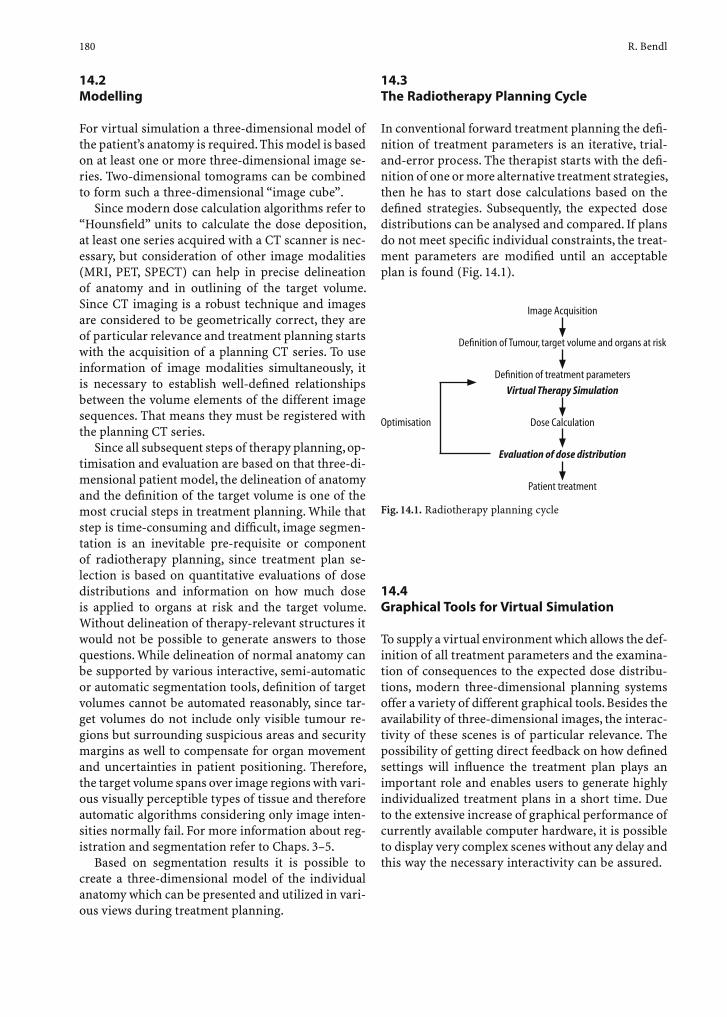
180 R. Bendl

14.2 Modelling

For virtual simulation a three-dimensional model of the patient’s anatomy is required. This model is based on at least one or more three-dimensional image se-ries. Two-dimensional tomograms can be combined to form such a three-dimensional “image cube”.

Since modern dose calculation algorithms refer to “Hounsfi eld” units to calculate the dose deposition, at least one series acquired with a CT scanner is nec-essary, but consideration of other image modalities (MRI, PET, SPECT) can help in precise delineation of anatomy and in outlining of the target volume. Since CT imaging is a robust technique and images are considered to be geometrically correct, they are of particular relevance and treatment planning starts with the acquisition of a planning CT series. To use information of image modalities simultaneously, it is necessary to establish well-defi ned relationships between the volume elements of the different image sequences. That means they must be registered with the planning CT series.

Since all subsequent steps of therapy planning, op-timisation and evaluation are based on that three-di-mensional patient model, the delineation of anatomy and the defi nition of the target volume is one of the most crucial steps in treatment planning. While that step is time-consuming and diffi cult, image segmen-tation is an inevitable pre-requisite or component of radiotherapy planning, since treatment plan se-lection is based on quantitative evaluations of dose distributions and information on how much dose is applied to organs at risk and the target volume. Without delineation of therapy-relevant structures it would not be possible to generate answers to those questions. While delineation of normal anatomy can be supported by various interactive, semi-automatic or automatic segmentation tools, defi nition of target volumes cannot be automated reasonably, since tar-get volumes do not include only visible tumour re-gions but surrounding suspicious areas and security margins as well to compensate for organ movement and uncertainties in patient positioning. Therefore, the target volume spans over image regions with vari-ous visually perceptible types of tissue and therefore automatic algorithms considering only image inten-sities normally fail. For more information about reg-istration and segmentation refer to Chaps. 3–5.

Based on segmentation results it is possible to create a three-dimensional model of the individual anatomy which can be presented and utilized in vari-ous views during treatment planning.

14.3 The Radiotherapy Planning Cycle

In conventional forward treatment planning the defi -nition of treatment parameters is an iterative, trial-and-error process. The therapist starts with the defi -nition of one or more alternative treatment strategies, then he has to start dose calculations based on the defi ned strategies. Subsequently, the expected dose distributions can be analysed and compared. If plans do not meet specifi c individual constraints, the treat-ment parameters are modifi ed until an acceptable plan is found (Fig. 14.1).

Fig. 14.1. Radiotherapy planning cycle

Image Acquisition

Defi nition of Tumour, target volume and organs at risk

Defi nition of treatment parameters

Virtual Therapy Simulation

Dose Calculation

Evaluation of dose distribution

Patient treatment

Optimisation

14.4 Graphical Tools for Virtual Simulation

To supply a virtual environment which allows the def-inition of all treatment parameters and the examina-tion of consequences to the expected dose distribu-tions, modern three-dimensional planning systems offer a variety of different graphical tools. Besides the availability of three-dimensional images, the interac-tivity of these scenes is of particular relevance. The possibility of getting direct feedback on how defi ned settings will infl uence the treatment plan plays an important role and enables users to generate highly individualized treatment plans in a short time. Due to the extensive increase of graphical performance of currently available computer hardware, it is possible to display very complex scenes without any delay and this way the necessary interactivity can be assured.

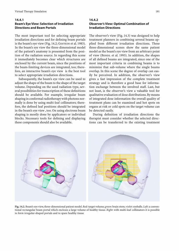
Virtual Therapy Simulation 181

14.4.2 Observer’s View: Optimal Combination of Irradiation Directions

The observer’s view (Fig. 14.3) was designed to help treatment planners in combining several beams ap-plied from different irradiation directions. These three-dimensional scenes show the same patient model as the beam’s eye view from an arbitrary point of view (Bendl et al. 1993). In addition, the shapes of all defi ned beams are integrated, since one of the most important criteria in combining beams is to minimize that sub-volume where the single beams overlap. In this scene the degree of overlap can eas-ily be perceived. In addition, the observer’s view gives a fast impression of the complete treatment strategy and is therefore a good base for informa-tion exchange between the involved staff. Last, but not least, is the observer’s view a valuable tool for qualitative evaluation of dose distributions. By means of integrated dose information the overall quality of treatment plans can be examined and hot spots on organs at risk or cold spots on the target volume can be detected easily.

During defi nition of irradiation directions the therapist must consider whether the selected direc-tions can be transferred to the existing treatment

Fig. 14.2. Beam’s eye view, three-dimensional patient model. Red: target volume; green: brain stem; violet: eyeballs. Left: a conven-tional rectangular beam portal which encloses a large volume of healthy tissue. Right: with multi-leaf collimators it is possible to form irregular-shaped portals and to spare healthy tissue

14.4.1 Beam’s Eye View: Selection of Irradiation Directions and Beam Portals

The most important tool for selecting appropriate irradiation directions and for defi ning beam portals is the beam’s eye view (Fig. 14.2; Goitein et al. 1983). In the beam’s eye view the three-dimensional model of the patient’s anatomy is presented from the posi-tion of the radiation source. In regarding this scene it immediately becomes clear which structures are enclosed by the current beam, since the positions of the beam-limiting devices are integrated, too; there-fore, an interactive beam’s eye view is the best tool to select appropriate irradiation directions.

Subsequently, the beam’s eye view can be used to adjust the shape of the beam to the shape of the target volume. Depending on the used radiation type, sev-eral possibilities for transcription of these defi nitions should be available. For example, irregular beam shaping in conformal radiotherapy with photons nor-mally is done by using multi-leaf collimators; there-fore, the defi ned leaf positions should be integrated in the beam’s eye view , too. On using electrons beam shaping is mostly done by applicators or individual blocks. Necessary tools for defi ning and displaying these components should also be available.

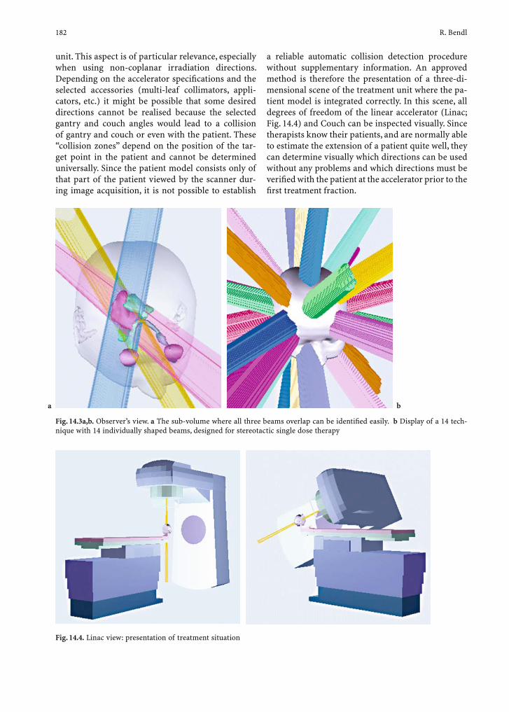
182 R. Bendl

unit. This aspect is of particular relevance, especially when using non-coplanar irradiation directions. Depending on the accelerator specifi cations and the selected accessories (multi-leaf collimators, appli-cators, etc.) it might be possible that some desired directions cannot be realised because the selected gantry and couch angles would lead to a collision of gantry and couch or even with the patient. These “collision zones” depend on the position of the tar-get point in the patient and cannot be determined universally. Since the patient model consists only of that part of the patient viewed by the scanner dur-ing image acquisition, it is not possible to establish

a reliable automatic collision detection procedure without supplementary information. An approved method is therefore the presentation of a three-di-mensional scene of the treatment unit where the pa-tient model is integrated correctly. In this scene, all degrees of freedom of the linear accelerator (Linac; Fig. 14.4) and Couch can be inspected visually. Since therapists know their patients, and are normally able to estimate the extension of a patient quite well, they can determine visually which directions can be used without any problems and which directions must be verifi ed with the patient at the accelerator prior to the fi rst treatment fraction.

Fig. 14.3a,b. Observer’s view. a The sub-volume where all three beams overlap can be identifi ed easily. b Display of a 14 tech-nique with 14 individually shaped beams, designed for stereotactic single dose therapy

ba

Fig. 14.4. Linac view: presentation of treatment situation

Virtual Therapy Simulation 183

14.4.3 Multi-planar Reconstructions of Tomographic Image Series

Besides artifi cial three-dimensional scenes, it is nec-essary to project selected irradiation directions and beam shapes onto the slices of the planning CT, too, to allow the examination of selected parameters on the originally acquired patient data. Of course, it is helpful to have not only projections on the initially acquired transversal slices but at least on multi-pla-nar reconstructions in the other two main directions (sagittal, coronal). The selection of oblique sections might be helpful during examination of dose distri-butions. Sometimes an additional gain of informa-tion can be achieved by projecting beams on images of other modalities, but this is usually considered to be of minor priority.

14.4.4 Digital Reconstructed Radiographs

Generation and presentation of digital reconstructed radiographs (DRRs) is a virtual simulation of real treatment simulators or portal imaging devices. Based on the information in the acquired CT image series it is possible to calculate artifi cial X-Ray im-ages from arbitrary directions comparable to those mentioned above (Galvin et al. 1995).

During X-Ray image acquisition, X-Rays are ab-sorbed differentially according to tissue density. Structures with high density (bones) absorb more intensity of the ray than soft tissue, which means that the incident radiation on the fi lm after having passed bony structures is low, resulting in a low optical den-sity on the fi lm (bright). Water, fat muscle tissue or air absorb only a small amount (or none) of the ra-diation. Rays running only through soft tissue keep a higher intensity which results in a high optical den-sity on the fi lm (dark or black).

To simulate these behaviours ray-tracing algorithms are used (see also Chap. 4.4.2). Starting from the posi-tion of the X-ray source, the algorithm traces a bundle of beams through an image cube, until a specifi ed pro-jection plane (i.e. the fi lm position) is reached (Siddon 1985). Each ray passes through different elements of the data cube (volume elements or voxel). Depending on how the values of the voxels passed through con-tribute to the fi nal value of the ray in the imaging plane, different kinds of images can be produced (Fig. 14.5).

If the absorption of a ray’s intensity is considered to be proportional to the density of a given voxel, the total absorption is proportional to the sum of the voxel densities along the ray. To generate DRRs, the voxel intensities must simply be summed (Fig. 14.5a). If an algorithm considers only the maximum voxel values along a ray and projects that value onto the image plane, maximum intensity projections (MIPs) can be generated. Applying such an algorithm to ap-

Fig. 14.5a–c. Principle of ray tracing. a Digital reconstructed radiographs. b Surface rendering. c Maximum intensity projection

b

a

c

184 R. Bendl

propriate image cubes (CT or MR angiographies), the blood vessel system can be visualised (Fig. 14.5b). Adding some constraints to the ray-tracing algorithm, e.g. the ray tracing should fi nish when a voxel with a particular intensity arrives, the surface of anatomical structures can be detected and visualized. As a pre-requisite, the intensity of those structures must have good contrast with respect to the surrounding tissue. In this way, the patient’s surface and bony structures can easily be visualised (Fig. 14.5c). Images generated with surface-rendering methods from the position of the radiation source show the same geometrical rela-tions as the beam’s eye view images explained above.

For radiotherapy, DRRs and MIPs are especially important. The MIPs can be used for detecting mal-formations of blood vessels (AVMs). The DRRs can help during patient positioning and positioning con-trol. Based on the specifi ed treatment parameters and the known geometry of the X-ray imaging systems, DRRs can be pre-calculated. To verify patient posi-tioning X-ray images can be acquired prior or during treatment. They can be compared to the calculated DRRs, deviations between both images can be calcu-lated automatically and it is possible to compensate for displacements by correcting the treatment posi-tion to the planned one.

On comparing DRRs with portal images generated with the beam of the treatment unit it is necessary to take care of different imaging energies. The CT images are normally acquired with an imaging energy in the lower kV range, the energy used for irradiation of pho-tons is in the range of 6–20 MV. Mega-voltage images usually show a much lower contrast, and it is diffi cult to perceive soft tissue structures. Due to those differences, a comparison of artifi cial images with verifi cation im-ages is often diffi cult, too. A solution could be the con-sideration of different mean image energies (Mohan and Chen 1985) already on generation of the DRRs.

14.5 Tools for Evaluating Dose Distributions

An optimal virtual simulator would not only present the result of geometrical changes (beam directions, shapes, etc.) immediately, but also the consequences on the expected dose distribution in real-time. Admittedly, the immediate feedback can be assured only on the geometrical aspects of treatment param-eters. Up to now it is still not possible to display the consequences of changed settings on dose distribu-tions in real-time on standard computer hardware.

Nevertheless, the possibility of examination and evaluation of dose distributions should be an integral part of a virtual simulator, since only the resulting dose distribution can answer the question, whether the selected treatment strategy considers all individ-ual constraints suffi ciently.

There is a large variety on methods to display dose information. By integrating dose distributions into the three-dimensional patient model, presented in the observer’s view, a fast impression about the global dose distribution can be achieved. This integration can be done with different techniques. Figure 14.6 shows two examples. On the left side dose informa-tion is integrated as iso-dose ribbons, which means that sub-volume which receives a dose higher than a given level is enclosed by some yellow ribbons. This way a planner can immediately verify whether the target volume is enclosed completely by the thera-peutic dose level. On the right side, the surface dose is displayed. That means the surfaces of all defi ned structures are coloured according to the expected dose. Black and blue areas do not receive any or only a small amount of dose; in red areas the dose is equal to the desired therapeutic dose level. This way, hot spots on organs at risk (here, for example, on the chi-asm and on the right optical nerve) or cold spots in the target volume (here in the topmost region) can be detected very easily.

Of course variations of these techniques are com-mon, too. For example, some treatment planning systems offer the possibility to display dose clouds as semi-transparent surfaces or are using more ad-vanced display techniques such as fog.

While those 3D scenes give a very fast impression of dose distributions, they are not suffi cient to get precise information about the dose distribution in-side of an organ at risk or in the target volume, since the patient model is reduced to the surface of ana-tomical structures and dose clouds. Therefore, most of the available radiotherapy simulators and planning systems supply possibilities to project dose informa-tion onto the initially acquired images. Again, various different techniques are possible. The most common techniques are the display of dose distributions as iso-dose lines, and the integration of dose informa-tion using colour-wash techniques (see Fig. 14.8: comparison of concurrent treatment plans.). An im-portant feature is the ability to present dose not only on the original CT image slices but on multi-planar reconstructions and oblique sections, too. The pos-sibility to project dose not only on the planning CT but also on other available series of other imaging modalities is desirable.

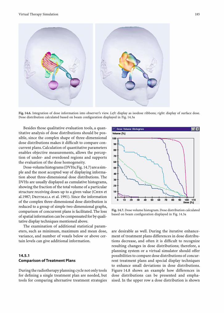
Virtual Therapy Simulation 185

Besides those qualitative evaluation tools, a quan-titative analysis of dose distributions should be pos-sible, since the complex shape of three-dimensional dose distributions makes it diffi cult to compare con-current plans. Calculation of quantitative parameters enables objective measurements, allows the percep-tion of under- and overdosed regions and supports the evaluation of the dose homogeneity.

Dose-volume histograms (DVHs; Fig. 14.7) are a sim-ple and the most accepted way of displaying informa-tion about three-dimensional dose distributions. The DVHs are usually displayed as cumulative histograms, showing the fraction of the total volume of a particular structure receiving doses up to a given value (Chen et al.1987; Drzymala et al. 1991). Since the information of the complex three-dimensional dose distribution is reduced to a group of simple two-dimensional graphs, comparison of concurrent plans is facilitated. The loss of spatial information can be compensated for by quali-tative display techniques mentioned above.

The examination of additional statistical param-eters, such as minimum, maximum and mean dose, variance, and number of voxels below or above cer-tain levels can give additional information.

14.5.1 Comparison of Treatment Plans

During the radiotherapy planning cycle not only tools for defi ning a single treatment plan are needed, but tools for comparing alternative treatment strategies

are desirable as well. During the iterative enhance-ment of treatment plans differences in dose distribu-tions decrease, and often it is diffi cult to recognize resulting changes in dose distributions; therefore, a planning system or a virtual simulator should offer possibilities to compare dose distributions of concur-rent treatment plans and special display techniques to enhance small deviations in dose distributions. Figure 14.8 shows an example how differences in dose distributions can be presented and empha-sised. In the upper row a dose distribution is shown

Fig. 14.6. Integration of dose information into observer’s view. Left: display as isodose ribbons; right: display of surface dose. Dose distribution calculated based on beam confi guration displayed in Fig. 14.3a

Fig. 14.7. Dose volume histogram. Dose distribution calculated based on beam confi guration displayed in Fig. 14.3a

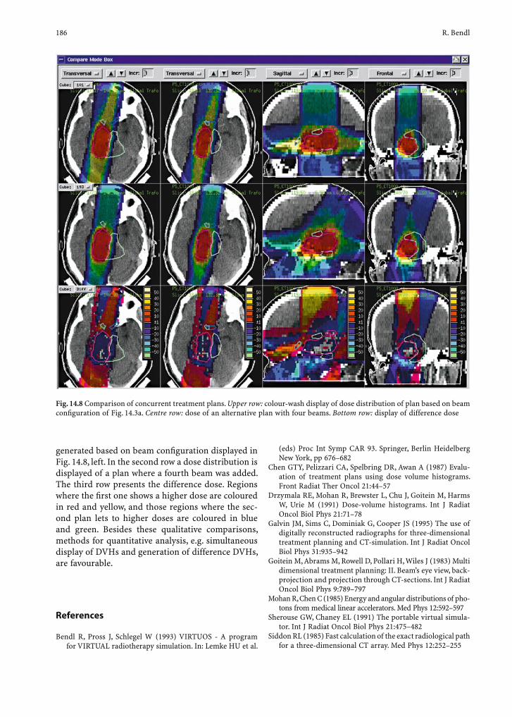
186 R. Bendl

generated based on beam confi guration displayed in Fig. 14.8, left. In the second row a dose distribution is displayed of a plan where a fourth beam was added. The third row presents the difference dose. Regions where the fi rst one shows a higher dose are coloured in red and yellow, and those regions where the sec-ond plan lets to higher doses are coloured in blue and green. Besides these qualitative comparisons, methods for quantitative analysis, e.g. simultaneous display of DVHs and generation of difference DVHs, are favourable.

References

Bendl R, Pross J, Schlegel W (1993) VIRTUOS - A program for VIRTUAL radiotherapy simulation. In: Lemke HU et al.

(eds) Proc Int Symp CAR 93. Springer, Berlin Heidelberg New York, pp 676–682

Chen GTY, Pelizzari CA, Spelbring DR, Awan A (1987) Evalu-ation of treatment plans using dose volume histograms. Front Radiat Ther Oncol 21:44–57

Drzymala RE, Mohan R, Brewster L, Chu J, Goitein M, Harms W, Urie M (1991) Dose-volume histograms. Int J Radiat Oncol Biol Phys 21:71–78

Galvin JM, Sims C, Dominiak G, Cooper JS (1995) The use of digitally reconstructed radiographs for three-dimensional treatment planning and CT-simulation. Int J Radiat Oncol Biol Phys 31:935–942

Goitein M, Abrams M, Rowell D, Pollari H, Wiles J (1983) Multi dimensional treatment planning: II. Beam’s eye view, back-projection and projection through CT-sections. Int J Radiat Oncol Biol Phys 9:789–797

Mohan R, Chen C (1985) Energy and angular distributions of pho-tons from medical linear accelerators. Med Phys 12:592–597

Sherouse GW, Chaney EL (1991) The portable virtual simula-tor. Int J Radiat Oncol Biol Phys 21:475–482

Siddon RL (1985) Fast calculation of the exact radiological path for a three-dimensional CT array. Med Phys 12:252–255

Fig. 14.8 Comparison of concurrent treatment plans. Upper row: colour-wash display of dose distribution of plan based on beam confi guration of Fig. 14.3a. Centre row: dose of an alternative plan with four beams. Bottom row: display of difference dose

Dose Calculation Algorithms 187

15 Dose Calculation Algorithms

Uwe Oelfke and Christian Scholz

U. Oelfke, PhDDeutsches Krebsforschungszentrum, Im Neuenheimer Feld 280, 69120 Heidelberg, GermanyC. Scholz, PhDSiemens Medical Solutions, Oncology Care Systems, Hans-Bunte-Str. 19, 69123 Heidelberg, Germany

15.1 Introduction

The accurate and fast calculation of a 3D dose distri-bution within the patient is one of the most central procedures in modern radiation oncology. It creates the only reliable and verifi able link between the cho-sen treatment parameters, and the observed clinical outcome for a specifi ed treatment technique, i.e., the prescribed dose level for the tumor, the number of therapeutic beams, their angles of incidence, and a set of intensity amplitudes – obtained by a careful treatment plan optimization – result in a distribution of absorbed dose which is the primary physical quan-tity available for an analysis of the achieved clinical

effects of this specifi c treatment. The twofold appli-cation of dose calculation algorithms in radiation oncology practice, fi rstly for the plan optimization in the treatment planning process, and secondly for the retrospective analysis of the correlation between treatment parameters and clinical outcome, defi nes two mutually confl icting goals of the respective dose algorithms. Firstly, the dose calculation has to be fast such that the treatment planning process can be completed in clinically acceptable time frames, and secondly, the result of the dose calculation has to be suffi ciently accurate so that the establishment of correlations between delivered dose and clinical effects remains reliable and meaningful. The confl ict between “high speed” and “high accuracy” is one of the crucial challenges for the development of modern dose calculation algorithms.

The accuracy of the dose calculation algorithms becomes a problem only for very heterogeneous tis-sues, where a very detailed modeling of the energy transport in the patient is required. The prediction of the dose around air cavities, e.g., often encountered for tumors adjacent to the paranasal sinuses or for solid tumors embedded in lung tissue, is intricate and time-consuming. Almost all new developments related to dose algorithms are specifi cally concen-trating on these or equivalent areas of tissue hetero-geneities, whereas for the majority of clinical cases with almost homogeneous tissues existing, simple calculation methods can be reliably applied.

Naturally, dose algorithms for high-energy photon beams were fi rst developed for the ultimate “homo-geneous” patient – a patient completely consisting of water (Schoknecht 1967). Measurements of a set of generic dose functions, e.g., tissue air ratios, tissue phantom ratios, output factors, and off-axis ratios, are measured in a water phantom for a set of regular treatment fi elds under reference conditions. The dose within a patient is then calculated by extrapolating these measurements to the specifi c chosen treatment fi elds and by the application of various correction al-gorithms, e.g., for the inclusion of missing tissues at the patient surface or the approximate consideration

CONTENTS

15.1 Introduction 18715.2 Model-Based Algorithms 18815.3 Modeling of the Primary Photon Fluence 18915.4 Dose Calculation in Homogeneous Media 19015.4.1 TERMA 19015.4.2 Dose Kernels: Point-Spread Kernel and Pencil Beam 19015.4.3 Superposition and Convolution Algorithms 19115.5 Accounting for Tissue Inhomogeneities 19115.5.1 Pencil Beam and Pathlength Scaling 19215.5.2 Density Scaling of Point-Spread Kernels 19215.5.3 Collapsed Cone and Kernel Tilting 19215.5.4 A Simple Example: Doses at Cork–Water Interfaces 19315.6 Dose Calculations and IMRT Optimization 19415.6.1 The Systematic Error 19415.6.2 The Convergence Error 19415.7 Conclusion 195 References 196

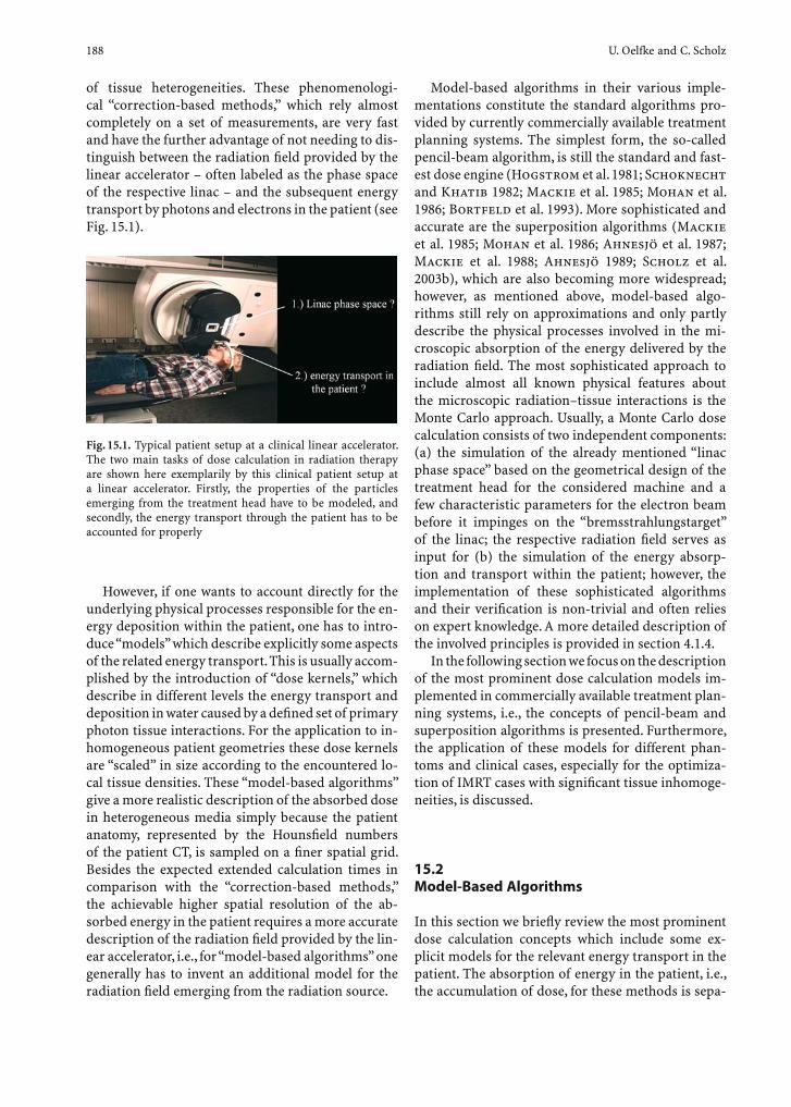
188 U. Oelfke and C. Scholz

of tissue heterogeneities. These phenomenologi-cal “correction-based methods,” which rely almost completely on a set of measurements, are very fast and have the further advantage of not needing to dis-tinguish between the radiation fi eld provided by the linear accelerator – often labeled as the phase space of the respective linac – and the subsequent energy transport by photons and electrons in the patient (see Fig. 15.1).

Model-based algorithms in their various imple-mentations constitute the standard algorithms pro-vided by currently commercially available treatment planning systems. The simplest form, the so-called pencil-beam algorithm, is still the standard and fast-est dose engine (Hogstrom et al. 1981; Schoknecht and Khatib 1982; Mackie et al. 1985; Mohan et al. 1986; Bortfeld et al. 1993). More sophisticated and accurate are the superposition algorithms (Mackie et al. 1985; Mohan et al. 1986; Ahnesjö et al. 1987; Mackie et al. 1988; Ahnesjö 1989; Scholz et al. 2003b), which are also becoming more widespread; however, as mentioned above, model-based algo-rithms still rely on approximations and only partly describe the physical processes involved in the mi-croscopic absorption of the energy delivered by the radiation fi eld. The most sophisticated approach to include almost all known physical features about the microscopic radiation–tissue interactions is the Monte Carlo approach. Usually, a Monte Carlo dose calculation consists of two independent components: (a) the simulation of the already mentioned “linac phase space” based on the geometrical design of the treatment head for the considered machine and a few characteristic parameters for the electron beam before it impinges on the “bremsstrahlungstarget” of the linac; the respective radiation fi eld serves as input for (b) the simulation of the energy absorp-tion and transport within the patient; however, the implementation of these sophisticated algorithms and their verifi cation is non-trivial and often relies on expert knowledge. A more detailed description of the involved principles is provided in section 4.1.4.

In the following section we focus on the description of the most prominent dose calculation models im-plemented in commercially available treatment plan-ning systems, i.e., the concepts of pencil-beam and superposition algorithms is presented. Furthermore, the application of these models for different phan-toms and clinical cases, especially for the optimiza-tion of IMRT cases with signifi cant tissue inhomoge-neities, is discussed.

15.2 Model-Based Algorithms

In this section we briefl y review the most prominent dose calculation concepts which include some ex-plicit models for the relevant energy transport in the patient. The absorption of energy in the patient, i.e., the accumulation of dose, for these methods is sepa-

However, if one wants to account directly for the underlying physical processes responsible for the en-ergy deposition within the patient, one has to intro-duce “models” which describe explicitly some aspects of the related energy transport. This is usually accom-plished by the introduction of “dose kernels,” which describe in different levels the energy transport and deposition in water caused by a defi ned set of primary photon tissue interactions. For the application to in-homogeneous patient geometries these dose kernels are “scaled” in size according to the encountered lo-cal tissue densities. These “model-based algorithms” give a more realistic description of the absorbed dose in heterogeneous media simply because the patient anatomy, represented by the Hounsfi eld numbers of the patient CT, is sampled on a fi ner spatial grid. Besides the expected extended calculation times in comparison with the “correction-based methods,” the achievable higher spatial resolution of the ab-sorbed energy in the patient requires a more accurate description of the radiation fi eld provided by the lin-ear accelerator, i.e., for “model-based algorithms” one generally has to invent an additional model for the radiation fi eld emerging from the radiation source.

Fig. 15.1. Typical patient setup at a clinical linear accelerator. The two main tasks of dose calculation in radiation therapy are shown here exemplarily by this clinical patient setup at a linear accelerator. Firstly, the properties of the particles emerging from the treatment head have to be modeled, and secondly, the energy transport through the patient has to be accounted for properly

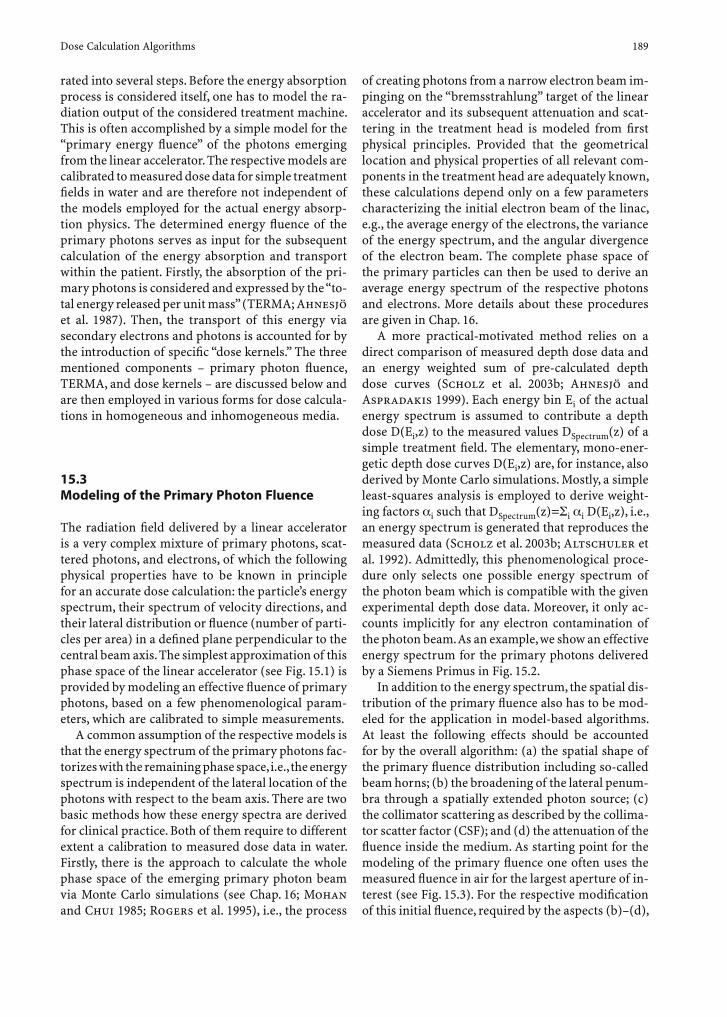
Dose Calculation Algorithms 189

rated into several steps. Before the energy absorption process is considered itself, one has to model the ra-diation output of the considered treatment machine. This is often accomplished by a simple model for the “primary energy fl uence” of the photons emerging from the linear accelerator. The respective models are calibrated to measured dose data for simple treatment fi elds in water and are therefore not independent of the models employed for the actual energy absorp-tion physics. The determined energy fl uence of the primary photons serves as input for the subsequent calculation of the energy absorption and transport within the patient. Firstly, the absorption of the pri-mary photons is considered and expressed by the “to-tal energy released per unit mass” (TERMA; Ahnesjö et al. 1987). Then, the transport of this energy via secondary electrons and photons is accounted for by the introduction of specifi c “dose kernels.” The three mentioned components – primary photon fl uence, TERMA, and dose kernels – are discussed below and are then employed in various forms for dose calcula-tions in homogeneous and inhomogeneous media.

15.3 Modeling of the Primary Photon Fluence

The radiation fi eld delivered by a linear accelerator is a very complex mixture of primary photons, scat-tered photons, and electrons, of which the following physical properties have to be known in principle for an accurate dose calculation: the particle’s energy spectrum, their spectrum of velocity directions, and their lateral distribution or fl uence (number of parti-cles per area) in a defi ned plane perpendicular to the central beam axis. The simplest approximation of this phase space of the linear accelerator (see Fig. 15.1) is provided by modeling an effective fl uence of primary photons, based on a few phenomenological param-eters, which are calibrated to simple measurements.

A common assumption of the respective models is that the energy spectrum of the primary photons fac-torizes with the remaining phase space, i.e., the energy spectrum is independent of the lateral location of the photons with respect to the beam axis. There are two basic methods how these energy spectra are derived for clinical practice. Both of them require to different extent a calibration to measured dose data in water. Firstly, there is the approach to calculate the whole phase space of the emerging primary photon beam via Monte Carlo simulations (see Chap. 16; Mohan and Chui 1985; Rogers et al. 1995), i.e., the process

of creating photons from a narrow electron beam im-pinging on the “bremsstrahlung” target of the linear accelerator and its subsequent attenuation and scat-tering in the treatment head is modeled from fi rst physical principles. Provided that the geometrical location and physical properties of all relevant com-ponents in the treatment head are adequately known, these calculations depend only on a few parameters characterizing the initial electron beam of the linac, e.g., the average energy of the electrons, the variance of the energy spectrum, and the angular divergence of the electron beam. The complete phase space of the primary particles can then be used to derive an average energy spectrum of the respective photons and electrons. More details about these procedures are given in Chap. 16.

A more practical-motivated method relies on a direct comparison of measured depth dose data and an energy weighted sum of pre-calculated depth dose curves (Scholz et al. 2003b; Ahnesjö and Aspradakis 1999). Each energy bin Ei of the actual energy spectrum is assumed to contribute a depth dose D(Ei,z) to the measured values DSpectrum(z) of a simple treatment fi eld. The elementary, mono-ener-getic depth dose curves D(Ei,z) are, for instance, also derived by Monte Carlo simulations. Mostly, a simple least-squares analysis is employed to derive weight-ing factors i such that DSpectrum(z)= i i D(Ei,z), i.e., an energy spectrum is generated that reproduces the measured data (Scholz et al. 2003b; Altschuler et al. 1992). Admittedly, this phenomenological proce-dure only selects one possible energy spectrum of the photon beam which is compatible with the given experimental depth dose data. Moreover, it only ac-counts implicitly for any electron contamination of the photon beam. As an example, we show an effective energy spectrum for the primary photons delivered by a Siemens Primus in Fig. 15.2.

In addition to the energy spectrum, the spatial dis-tribution of the primary fl uence also has to be mod-eled for the application in model-based algorithms. At least the following effects should be accounted for by the overall algorithm: (a) the spatial shape of the primary fl uence distribution including so-called beam horns; (b) the broadening of the lateral penum-bra through a spatially extended photon source; (c) the collimator scattering as described by the collima-tor scatter factor (CSF); and (d) the attenuation of the fl uence inside the medium. As starting point for the modeling of the primary fl uence one often uses the measured fl uence in air for the largest aperture of in-terest (see Fig. 15.3). For the respective modifi cation of this initial fl uence, required by the aspects (b)–(d),

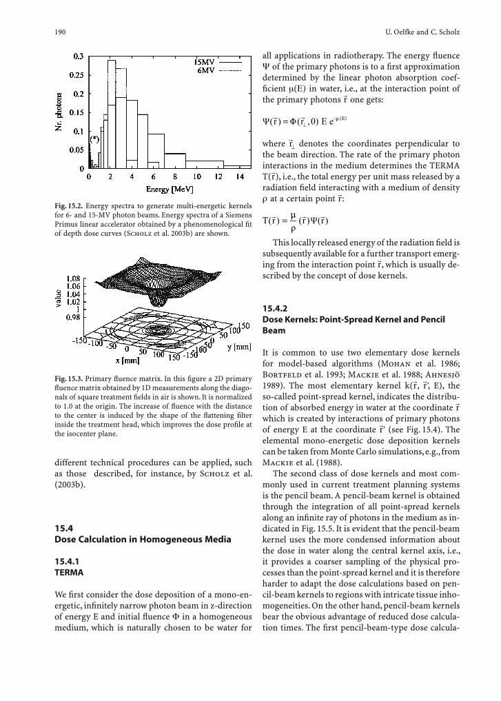
190 U. Oelfke and C. Scholz

different technical procedures can be applied, such as those described, for instance, by Scholz et al. (2003b).

15.4 Dose Calculation in Homogeneous Media

15.4.1 TERMA

We fi rst consider the dose deposition of a mono-en-ergetic, infi nitely narrow photon beam in z-direction of energy E and initial fl uence in a homogeneous medium, which is naturally chosen to be water for

all applications in radiotherapy. The energy fl uence of the primary photons is to a fi rst approximation

determined by the linear photon absorption coef-fi cient ( ) in water, i.e., at the interaction point of the primary photons

rr one gets:

Ψ Φ( , )r rr ) = (r E e- z⊥ 0 µ

where rr⊥ denotes the coordinates perpendicular to

the beam direction. The rate of the primary photon interactions in the medium determines the TERMA T(rr), i.e., the total energy per unit mass released by a

radiation fi eld interacting with a medium of density at a certain point

rr:

( (T r ) = r ) (r)r r rµρ

Ψ

This locally released energy of the radiation fi eld is subsequently available for a further transport emerg-ing from the interaction point

rr, which is usually de-scribed by the concept of dose kernels.

15.4.2 Dose Kernels: Point-Spread Kernel and Pencil Beam

It is common to use two elementary dose kernels for model-based algorithms (Mohan et al. 1986; Bortfeld et al. 1993; Mackie et al. 1988; Ahnesjö 1989). The most elementary kernel k(

rr, rr ', E), the

so-called point-spread kernel, indicates the distribu-tion of absorbed energy in water at the coordinate

rr which is created by interactions of primary photons of energy E at the coordinate

rr ' (see Fig. 15.4). The elemental mono-energetic dose deposition kernels can be taken from Monte Carlo simulations, e.g., from Mackie et al. (1988).

The second class of dose kernels and most com-monly used in current treatment planning systems is the pencil beam. A pencil-beam kernel is obtained through the integration of all point-spread kernels along an infi nite ray of photons in the medium as in-dicated in Fig. 15.5. It is evident that the pencil-beam kernel uses the more condensed information about the dose in water along the central kernel axis, i.e., it provides a coarser sampling of the physical pro-cesses than the point-spread kernel and it is therefore harder to adapt the dose calculations based on pen-cil-beam kernels to regions with intricate tissue inho-mogeneities. On the other hand, pencil-beam kernels bear the obvious advantage of reduced dose calcula-tion times. The fi rst pencil-beam-type dose calcula-

Fig. 15.3. Primary fl uence matrix. In this fi gure a 2D primary fl uence matrix obtained by 1D measurements along the diago-nals of square treatment fi elds in air is shown. It is normalized to 1.0 at the origin. The increase of fl uence with the distance to the center is induced by the shape of the fl attening fi lter inside the treatment head, which improves the dose profi le at the isocenter plane.

Fig. 15.2. Energy spectra to generate multi-energetic kernels for 6- and 15-MV photon beams. Energy spectra of a Siemens Primus linear accelerator obtained by a phenomenological fi t of depth dose curves (Scholz et al. 2003b) are shown.

(E)(E)

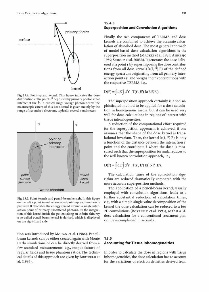
Dose Calculation Algorithms 191

tion was introduced by Mohan et al. (1986). Pencil-beam kernels can be either created again with Monte Carlo simulations or can be directly derived from a few standard measurements, e.g., output factors of regular fi elds and tissue phantom ratios. The techni-cal details of this approach are given by Bortfeld et al. (1993).

15.4.3 Superposition and Convolution Algorithms

Finally, the two components of TERMA and dose kernels are combined to achieve the accurate calcu-lation of absorbed dose. The most general approach of model-based dose calculation algorithms is the superposition method (Mackie et al. 1985; Ahnesjö 1989; Scholz et al. 2003b). It generates the dose deliv-ered at a point

rr by superimposing the dose contribu-tions from all dose kernels k(

rr, rr ', E) of the defi ned

energy spectrum originating from all primary inter-action points

rr ' and weighs their contributions with the respective TERMA, i.e.,

D(r ) = dE' d r' T r', E') k(r, r',E').3r r r r∫ ∫ (

The superposition approach certainly is a too so-phisticated method to be applied for a dose calcula-tion in homogenous media, but it can be used very well for dose calculations in regions of interest with tissue inhomogeneities.

A reduction of the computational effort required for the superposition approach, is achieved, if one assumes that the shape of the dose kernel is trans-lational invariant. Then, the kernel k(

rr, rr ', E) is only

a function of the distance between the interaction rr '

point and the coordinate rr where the dose is mea-

sured such that the superposition formula reduces to the well known convolution approach, i.e.,

r'D(r) = dE' d r' T r', E') k( r− ,E').3r r r r∫ ∫ (

The calculation times of the convolution algo-rithm are reduced dramatically compared with the more accurate superposition methods.

The application of a pencil-beam kernel, usually employed with convolution algorithms, leads to a further substantial reduction of calculation times, e.g., with a simple single value decomposition of the kernel the dose calculation can be reduced to a few 2D convolutions (Bortfeld et al. 1993), so that a 3D dose calculation for a conventional treatment plan can be accomplished in seconds.

15.5 Accounting for Tissue Inhomogeneities

In order to calculate the dose in regions with tissue inhomogeneities, the dose calculation has to account for the variations of electron densities derived from

Fig. 15.5. Point kernels and pencil-beam kernels. In this fi gure on the left a point kernel or so-called point-spread function is pictured. It describes the energy spread around a single inter-action point of primary unscattered photons. By the integra-tion of this kernel inside the patient along an infi nite thin ray a so-called pencil-beam kernel is derived, which is displayed on the right-hand side

Fig. 15.4. Point-spread kernel. This fi gure indicates the dose distribution at the points

rr deposited by primary photons that interact at the

rr '. In clinical mega-voltage photon beams the macroscopic extent of this dose kernel is given mainly by the range of secondary electrons, typically several centimeters

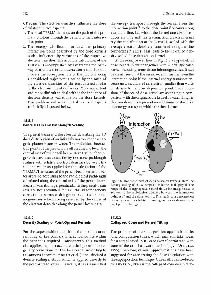
192 U. Oelfke and C. Scholz

CT scans. The electron densities infl uence the dose calculation in two aspects:1. The local TERMA depends on the path of the pri-

mary photons through the patient to their interac-tion point.

2. The energy distribution around the primary interaction point described by the dose kernels is also infl uenced by variations of the respective electron densities. The accurate calculation of the TERMA is accomplished by ray tracing the path-way of a photon to its interaction point. For this process the absorption rate of the photons along a considered trajectory is scaled by the ratio of the electron densities of the encountered media to the electron density of water. More important and more diffi cult to deal with is the infl uence of electron density variations on the dose kernels. This problem and some related practical aspects are briefl y discussed below.

15.5.1 Pencil Beam and Pathlength Scaling

The pencil beam is a dose kernel describing the 3D dose distribution of an infi nitely narrow mono-ener-getic photon beam in water. The individual interac-tion points of the photons are all assumed to be on the central axis of the pencil beam. Here tissue inhomo-geneities are accounted for by the same pathlength scaling with relative electron densities between tis-sue and water as applied for the calculation of the TERMA. The values of the pencil-beam kernel in wa-ter are used according to the radiological pathlength calculated along the central axis of the pencil beam. Electron variations perpendicular to the pencil-beam axis are not accounted for, i.e., this inhomogeneity correction assumes a slab geometry of tissue inho-mogeneities, which are represented by the values of the electron densities along the pencil-beam axis.

15.5.2 Density Scaling of Point-Spread Kernels

For the superposition algorithm the most accurate sampling of the primary interaction points within the patient is required. Consequently, this method also applies the most accurate technique of inhomo-geneity corrections for the dose kernel. According to O’Connor’s theorem, Mohan et al (1986) devised a density scaling method which is applied directly to the point-spread kernel. Basically, it is assumed that

the energy transport through the kernel from the interaction point

rr ' to the dose point rr occours along

a straight line, i.e., within the kernel one also intro-duces an “internal” ray tracing. Along each internal ray the contribution of the kernel is scaled with the average electron density encountered along the line connecting

rr ' and rr. This leads to the so-called den-

sity-scaled dose deposition kernels.As an example we show in Fig. 15.6 a hypothetical

dose kernel in water together with a density-scaled kernel including some tissue inhomogeneities. It can be clearly seen that the kernel extends further from the interaction point if the internal energy transport en-counters a medium of an electron smaller than water on its way to the dose deposition point. The dimen-sions of the scaled dose kernel are shrinking in com-parison with the original dose kernel in water if higher electron densities represent an additional obstacle for the energy transport within the dose kernel.

Fig. 15.6. Isodose curves of density-scaled kernels. Here the density-scaling of the Superposition kernel is displayed. The range of the energy spread behind tissue inhomogeneities is adapted to the radiological distance between the interaction point at

rr ' and the dose point rr. This leads to a deformation

of the isodose lines behind inhomogeneities as shown in the right part of the fi gure

15.5.3 Collapsed Cone and Kernel Tilting

The problem of the superposition approach are its long computation times, which may still take hours for a complicated IMRT case even if performed with state-of-the-art hardware technology (Schulze 1995); therefore, various approximations have been suggested for accelerating the dose calculation with the superposition technique. One method introduced by Ahnesjö (1989) is the collapsed cone-beam tech-

0 0

2> 0

1< 0

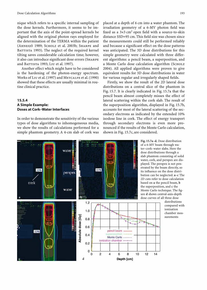
Dose Calculation Algorithms 193

nique which refers to a specifi c internal sampling of the dose kernels. Furthermore, it seems to be im-portant that the axis of the point-spread kernels be aligned with the original photon rays employed for the determination of the TERMA within the patient (Ahnesjö 1989; Scholz et al. 2003b; Sharpe and Battista 1993). The neglect of the required kernel tilting saves considerable calculation time; however, it also can introduce signifi cant dose errors (Sharpe and Battista 1993; Liu et al. 1997).

Another effect which might have to be considered is the hardening of the photon-energy spectrum. Works of Liu et al. (1997) and Metcalfe et al. (1990) showed that these effects are usually minimal in rou-tine clinical practice.

15.5.4 A Simple Example: Doses at Cork–Water Interfaces

In order to demonstrate the sensitivity of the various types of dose algorithms to inhomogeneous media, we show the results of calculations performed for a simple phantom geometry. A 4-cm slab of cork was

placed at a depth of 6 cm into a water phantom. The irradiation geometry of a 6-MV photon fi eld was fi xed as a 3×3 cm2 open fi eld with a source-to-skin distance SSD=95 cm. This fi eld size was chosen since the measurements could still be performed reliably and because a signifi cant effect on the dose patterns was anticipated. The 3D dose distributions for this simple geometry were calculated with three differ-ent algorithms: a pencil beam, a superposition, and a Monte Carlo dose calculation algorithm (Scholz 2004). All applied algorithms were proven to give equivalent results for 3D dose distributions in water for various regular and irregularly shaped fi elds.

Firstly, we show the result of the 2D lateral dose distributions on a central slice of the phantom in Fig. 15.7. It is clearly indicated in Fig. 15.7a that the pencil beam almost completely misses the effect of lateral scattering within the cork slab. The result of the superposition algorithm, displayed in Fig. 15.7b, accounts for most of the lateral scattering of the sec-ondary electrons as indicated by the extended 10% isodose line in cork. The effect of energy transport through secondary electrons is even more pro-nounced if the results of the Monte Carlo calculation, shown in Fig. 15.7c, are considered.

Fig. 15.7a–d. Dose distribution of a 6-MV beam through wa-ter–cork–water slabs. Here the dose distributions through a slab phantom consisting of solid water, cork, and perspex are dis-played. The perspex is not pen-etrated by the beam directly, so its infl uence on the dose distri-bution can be neglected. a–c The 2D cuts refer to dose calculation based on a the pencil beam, b the superposition, and c the Monte Carlo technique. The fi g-ure d shows central-axis-depth dose curves of all three dose

distributions compared with ionization chamber mea-surements

ba

c d

194 U. Oelfke and C. Scholz

These results are consistent with the respective depth-dose curves shown in Fig 15.7d. The enhanced lateral scattering of secondary electrons in the low-density medium reduces the dose values on the cen-tral-beam axis, an effect which is almost completely missed by the pencil-beam calculation resulting in a severe overestimation of the respective dose of up to 12% of the maximum dose. This discrepancy is sub-stantially reduced by the superposition algorithm. Only the Monte Carlo calculation was able to reproduce the experimental data with an accuracy of 2%, which was the estimated accuracy of the measurement.

While these simple phantom experiments may re-veal some generic features of the discussed dose cal-culation algorithms, it is not clear to what extent the various algorithms generate dose differences which are of clinical relevance.

In the fi nal section of this review we address this issue briefl y by considering the infl uence of different dose calculation engines on IMRT dose optimization for clinical cases with abundant severe tissue inho-mogeneities.

15.6 Dose Calculations and IMRT Optimization

The role of advanced high-energy photon dose calcu-lations for iterative IMRT treatment planning is still under investigation. Since conventional algorithms, such as pencil-beam methods with poor consider-ation of inhomogeneities, could produce substantial deviations in media different to water, the quality of intensity-modulated treatment plans generated through those dose calculation methods was re-cently reviewed by different groups (Jeraj et al. 2002; Siebers et al. 2001, 2002; Scholz et al. 2003a).

Particularly two aspects are important referring to dose calculation in IMRT: fi rstly, one has to assess the accuracy of the respective algorithm as required for the determination and evaluation of the fi nal dose pattern originating from a given set of fl uence ampli-tudes. Deviations from a reference dose calculation can be called systematic errors. Secondly, the infl uence of the dose algorithm in the optimization process itself should be analyzed, since deviations in the dose calcu-lation induces differences in bixel intensities in the fl u-ence maps, which is usually referred to as convergence error. In order to demonstrate the nature of these two errors, we consider one of the most sensitive clinical cases with respect to dose calculations, the irradiation of small, solid lesions embedded in lung tissue.

15.6.1 The Systematic Error

As mentioned previously, the systematic error indi-cates the difference in dose which arises from the application of different dose calculation algorithms for a given set of fl uence matrices. A solid lung tu-mor of about 30-mm diameter located in the left lung is totally surrounded by low-density lung tissue. It is irradiated with fi ve coplanar, intensity-modu-lated beams. As indicated by the dose distribution on a transversal CT slice of the patient in Fig. 15.8a, the original optimization based on the pencil-beam dose calculation seems to cover well the PTV by the prescribed dose of 63 Gy (100% isodose); however, the recalculation with the superposition algorithm shown in Fig. 15.8b reveals that only a small volume of the target is encompassed by the 60 Gy isodose (95% isodose) and that a severe underdosage of about 13 Gy in mean dose is observed for the PTV.

The systematic error induced by the pencil-beam algorithm demonstrates that this dose calculation method severely overestimates the dose inside the tumor. For the considered case the respective un-derdosage of the tumor shown by the superposition algorithm is based on the fact that for high-energy photon fi elds the range of many secondary electrons is larger than the radius of the tumor volume shown above; thus, there is not enough material to absorb the total number of secondary electrons inside the target region. The remaining electrons simply are scattered into the low-density lung tissue. These fi ndings are also well represented by the dose-volume histogram shown in Fig. 15.8d.

15.6.2 The Convergence Error

The convergence error is defi ned by the dose differ-ence which arises from the application of two dif-ferent fl uence matrices – obtained by inverse plan-ning with two different dose algorithms – for which the same reference dose calculation is applied. For our example we compare the dose distributions in Fig. 15.8b, where the pencil-beam algorithm was used for the generation of the fl uence matrices, and the dose distribution in Fig. 15.8c, where the superposi-tion algorithm was employed for the optimization. Once the fl uence matrices were established, the fi nal dose distributions were obtained by a calculation with the superposition algorithm. As clearly indicated by the fl uence matrices shown in Fig. 15.9, the optimiza-

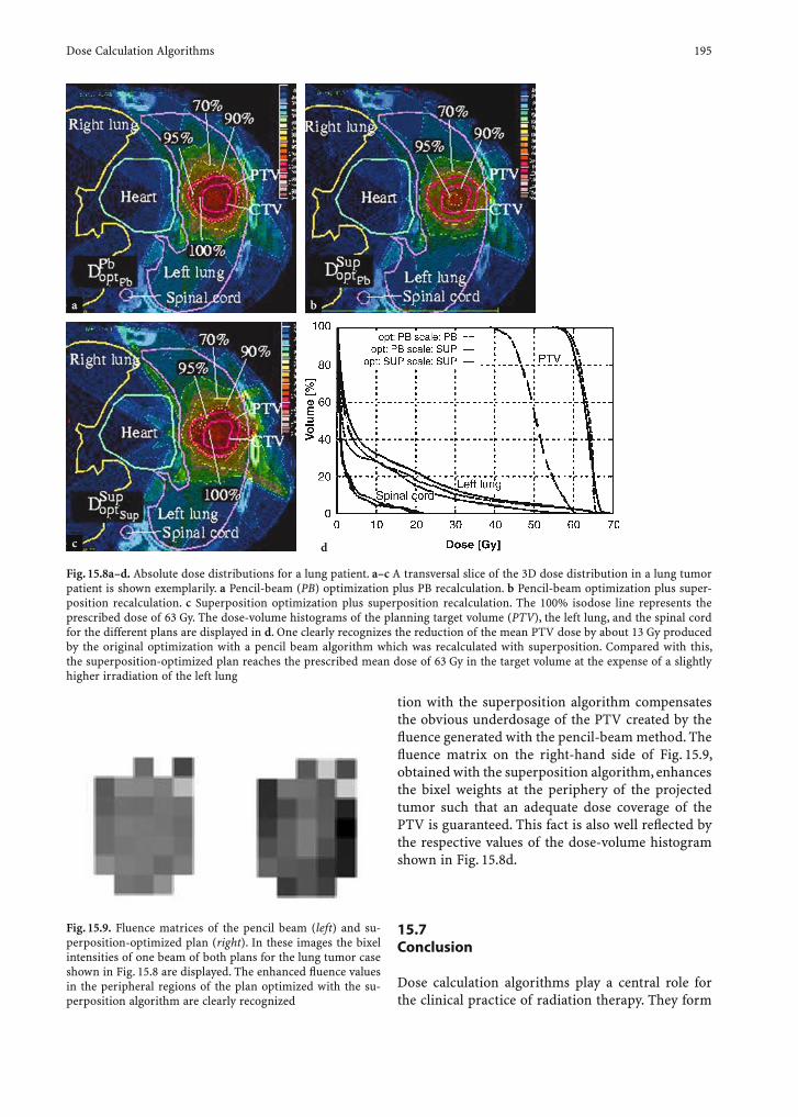
Dose Calculation Algorithms 195

tion with the superposition algorithm compensates the obvious underdosage of the PTV created by the fl uence generated with the pencil-beam method. The fl uence matrix on the right-hand side of Fig. 15.9, obtained with the superposition algorithm, enhances the bixel weights at the periphery of the projected tumor such that an adequate dose coverage of the PTV is guaranteed. This fact is also well refl ected by the respective values of the dose-volume histogram shown in Fig. 15.8d.

15.7 Conclusion

Dose calculation algorithms play a central role for the clinical practice of radiation therapy. They form

Fig. 15.8a–d. Absolute dose distributions for a lung patient. a–c A transversal slice of the 3D dose distribution in a lung tumor patient is shown exemplarily. a Pencil-beam (PB) optimization plus PB recalculation. b Pencil-beam optimization plus super-position recalculation. c Superposition optimization plus superposition recalculation. The 100% isodose line represents the prescribed dose of 63 Gy. The dose-volume histograms of the planning target volume (PTV), the left lung, and the spinal cord for the different plans are displayed in d. One clearly recognizes the reduction of the mean PTV dose by about 13 Gy produced by the original optimization with a pencil beam algorithm which was recalculated with superposition. Compared with this, the superposition-optimized plan reaches the prescribed mean dose of 63 Gy in the target volume at the expense of a slightly higher irradiation of the left lung

Fig. 15.9. Fluence matrices of the pencil beam (left) and su-perposition-optimized plan (right). In these images the bixel intensities of one beam of both plans for the lung tumor case shown in Fig. 15.8 are displayed. The enhanced fl uence values in the peripheral regions of the plan optimized with the su-perposition algorithm are clearly recognized

d

ba

c

196 U. Oelfke and C. Scholz

the basis for any treatment plan optimization, a fea-ture which becomes increasingly important with the development of complex treatment techniques such as IMRT. The role of highly accurate and therefore mostly time-consuming dose algorithms, such as su-perposition algorithms or Monte Carlo simulations, in clinical radiation therapy is still under investi-gation. Their increased accuracy offers substantial advantages for clinical cases which involve intricate tissue inhomogeneities.

Even if in many radiotherapy centers the treatment plans are still based on the pencil-beam method, its general applicability to inhomogeneous clinical cases has to be questioned. On the other hand, inside quite homogeneous regions, as in the central head region or the abdomen, the pencil beam generates dose distributions with excellent precision and provides the best trade-off between accuracy and calculation times.

In the case of severe tissue inhomogeneities the superposition method produces dose distributions which fairly cover the target region, even if minor differences are observed in comparison with Monte Carlo calculations. These offer the best prediction of the deposited dose inside arbitrary tissue types. Some Monte Carlo-based programs already offer computation times comparable to those of superpo-sition algorithms, and therefore their applicability in clinical practice will probably further increase for a small and special class of clinical cases.

References

Ahnesjö A (1989) Collapsed cone convolution of radiant energy for photon dose calculation in heterogeneous media. Med Phys 16:577–592

Ahnesjö A, Aspradakis MM (1999) Dose calculations for external photon beams in radiotherapy. Phys Med Biol 44:R99–R155

Ahnesjö A, Andreo P, Brahme A (1987) Calculation and appli-cation of point spread functions for treatment planning with high energy photon beams. Acta Oncol 26:49–56

Altschuler MD, Bloch P, Buhle EL, Ayyalasomayajula S (1992) 3D dose calculation for electron and photon beams. Phys Med Biol 37:391–411

Bortfeld T, Schlegel W, Rhein B (1993) Decomposition of pencil beam kernels for fast dose calculations in three-dimensional treatment planning. Med Phys 20:311–318

Hogstrom KR, Mills MD, Almond PR (1981) Electron beam dose calculations. Phys Med Biol 26:445–459

Jeraj R, Keall PJ, Siebers JV (2002) The effect of dose calcu-lation accuracy on inverse treatment planning. Phys Med Biol 47:391–407

Liu HH, Mackie TR, McCullough EC (1997) Correcting kernel tilting and hardening in convolution/superposition dose calculations for clinical divergent and polychromatic photon beams. Med Phys 24:1729–1741

Mackie TR, Scrimger JW, Battista JJ (1985) A convolution method of calculating dose for 15 MV X-ray. Med Phys 12:188–197

Mackie TR, Bielajew AF, Rogers DW, Battista JJ (1988) Genera-tion of photon energy deposition kernels using the EGS Monte Carlo code. Phys Med Biol 33:1–20

Metcalfe PE, Hoban PW, Murray DC, Round WH (1990) Beam hardening of 10-MV radiotherapy X-rays: analysis using a convolution/superposition method. Phys Med Biol 35:1533–1549

Mohan R, Chui C (1985) Energy and angular distributions of photons from medical linear accelerators. Med Phys 12:592–597

Mohan R, Chui C, Lidofsky L (1986) Differential pencil beam dose computation model for photons. Med Phys 13:64–73

Rogers DWO, Faddegon BA, Ding GX, Ma C-M, We J, Mackie TR (1995) BEAM: a Monte Carlo code to simulate radio-therapy treatment units. Med Phys 22:503–524

Schoknecht G (1967) Description of radiation fi elds by separa-tion of primary and scatter radiation. I. The tissue–air ratio in 60Co fi elds. Strahlentherapie 132:516–528

Schoknecht G, Khatib M (1982) Model calculations of the energy distribution of scattered radiation in a patient (author’s transl). Röntgenblätter 35:303–306

Scholz C (2004) Development and evaluation of advanced dose calculations for modern radiation therapy. PhD thesis, Uni-versity of Heidelberg

Scholz C, Nill S, Oelfke U (2003a) Comparison of IMRT opti-mization based on a pencil beam and a superposition algo-rithm. Med Phys 30:1909–1913

Scholz C, Schulze C, Oelfke U, Bortfeld T (2003b) Development and clinical application of a fast superposition algorithm in radiation therapy. Radiother Oncol 69:79–90

Schulze C (1995) Entwicklung schneller Algorihmen zur Dosis-berechnung für die Bestrahlung inhomogener Medien mit hochenergetischen Photonen. PhD thesis, DKFZ, Heidel-berg

Sharpe MB, Battista JJ (1993) Dose calculations using con-volution and superposition principles: the orientation of dose spread kernels in divergent X-ray beams. Med Phys 20:1685–1694

Siebers JV, Tong S, Lauterbach M, Wu Q, Mohan R (2001) Accel-eration of dose calculations for intensity-modulated radio-therapy. Med Phys 28:903–910

Siebers JV, Lauterbach M, Tong S, Wu Q, Mohan R (2002) Reducing dose calculation time for accurate iterative IMRT planning. Med Phys 29:231–237

Monte Carlo Dose Calculation for Treatment Planning 197

16 Monte Carlo Dose Calculation for Treatment Planning

Matthias Fippel

M. Fippel, PhDUniversitätsklinik für Radioonkologie, Medizinische Physik, Universitätsklinikum Tübingen, Hoppe-Seyler-Strasse 3, 72076 Tübingen, Germany

16.1 Introduction

To calculate the dose in human tissue caused by ion-izing radiation one has to solve a complex equation, the so-called transport equation. This equation is different for each patient and is also dependent on the treatment conditions, i.e. fi eld size, fi eld shape, energy of the radiation, beam direction, behaviour of the irradiation device, etc. There are two classes of calculation methods to solve the transport equa-tion, direct and indirect methods. Indirect methods (see Chap. 15) start with a known solution of the transport equation, e.g. a measured dose distribution in water. This distribution is then corrected to take into account the beam confi guration and the tissue inhomogeneities of the patient. Direct methods cal-culate dose distributions numerically by solving the

transport equation explicitly. The patient geometry is modelled by a three-dimensional distribution of tissue types based on a set of CT images. The par-ticle fl uence of photons and electrons at the patient’s surface is taken into account by a model of the treat-ment device, e.g. a model of the linear accelerator head. Direct methods are pencil-beam (see Chap. 15), collapsed cone (see Chap. 15) and Monte Carlo (MC) algorithms.

Pencil-beam and collapsed-cone algorithms are different implementations of the superposition/con-volution technique. They are based on various ap-proximations and simplifi cations, such as:• The modelling of the treatment device by simple

sources, e.g. point sources or parallel sources• The modelling of electron transport on straight

lines• The neglect or simplifi ed modelling of the lateral

density scaling in the case of pencil-beam algo-rithms (slab approximation)

• The discretisation of the point-spread function (energy kernel) in the case of collapsed-cone algo-rithms

• The neglect or approximate representation of the energy kernel tilt angle in order to reduce compu-tation time

• The neglect or estimation of effects such as depth hardening and off-axis softening

Usually, these techniques provide results within seconds. On the other hand, dose calculation can be incorrect especially in the head, neck and thorax regions because of the approximations used. As an example, the dose distribution of a 12-MeV electron beam with bolus in a patient with mammary-gland carcinoma is calculated with Monte Carlo and the pencil-beam algorithm of a commercial treatment planning system (see Fig. 16.1). The MC-generated dose distribution (Fig. 16.1a) shows the infl uence of low density tissue (lung) on the range of the elec-trons; however, the electron range is underestimated if a pencil-beam algorithm is used for dose calcula-tion. This effect is demonstrated clearly by the cor-

CONTENTS

16.1 Introduction 19716.2 Concept of Monte Carlo Integration 19816.3 Photon Transport Simulation 19916.4 Electron Transport Simulation 19916.5 Statistical Noise and Variance Reduction Techniques 20016.6 Material Parameters 20116.7 Beam Modelling 20216.8 Monte Carlo Dose Engines 20316.9 Monte Carlo Dose Calculation for Inverse Planning and IMRT 20416.10 Monte Carlo Dose Calculation for Ion Beam Therapy 205 References 205

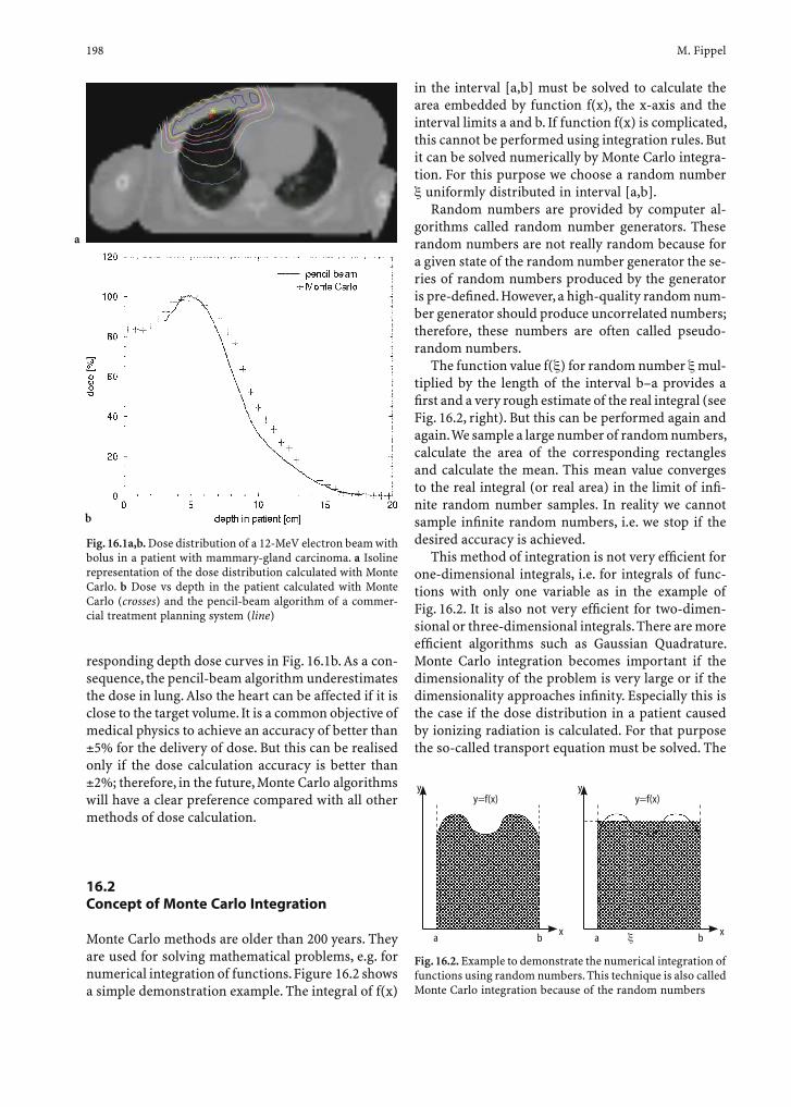
198 M. Fippel

Fig. 16.1a,b. Dose distribution of a 12-MeV electron beam with bolus in a patient with mammary-gland carcinoma. a Isoline representation of the dose distribution calculated with Monte Carlo. b Dose vs depth in the patient calculated with Monte Carlo (crosses) and the pencil-beam algorithm of a commer-cial treatment planning system (line)

a

b

Fig. 16.2. Example to demonstrate the numerical integration of functions using random numbers. This technique is also called Monte Carlo integration because of the random numbers

a b a

y yy=f(x)y=f(x)

bx x

in the interval [a,b] must be solved to calculate the area embedded by function f(x), the x-axis and the interval limits a and b. If function f(x) is complicated, this cannot be performed using integration rules. But it can be solved numerically by Monte Carlo integra-tion. For this purpose we choose a random number

uniformly distributed in interval [a,b].Random numbers are provided by computer al-

gorithms called random number generators. These random numbers are not really random because for a given state of the random number generator the se-ries of random numbers produced by the generator is pre-defi ned. However, a high-quality random num-ber generator should produce uncorrelated numbers; therefore, these numbers are often called pseudo-random numbers.

The function value f( ) for random number mul-tiplied by the length of the interval b–a provides a fi rst and a very rough estimate of the real integral (see Fig. 16.2, right). But this can be performed again and again. We sample a large number of random numbers, calculate the area of the corresponding rectangles and calculate the mean. This mean value converges to the real integral (or real area) in the limit of infi -nite random number samples. In reality we cannot sample infi nite random numbers, i.e. we stop if the desired accuracy is achieved.

This method of integration is not very effi cient for one-dimensional integrals, i.e. for integrals of func-tions with only one variable as in the example of Fig. 16.2. It is also not very effi cient for two-dimen-sional or three-dimensional integrals. There are more effi cient algorithms such as Gaussian Quadrature. Monte Carlo integration becomes important if the dimensionality of the problem is very large or if the dimensionality approaches infi nity. Especially this is the case if the dose distribution in a patient caused by ionizing radiation is calculated. For that purpose the so-called transport equation must be solved. The

responding depth dose curves in Fig. 16.1b. As a con-sequence, the pencil-beam algorithm underestimates the dose in lung. Also the heart can be affected if it is close to the target volume. It is a common objective of medical physics to achieve an accuracy of better than ±5% for the delivery of dose. But this can be realised only if the dose calculation accuracy is better than ±2%; therefore, in the future, Monte Carlo algorithms will have a clear preference compared with all other methods of dose calculation.

16.2 Concept of Monte Carlo Integration

Monte Carlo methods are older than 200 years. They are used for solving mathematical problems, e.g. for numerical integration of functions. Figure 16.2 shows a simple demonstration example. The integral of f(x)

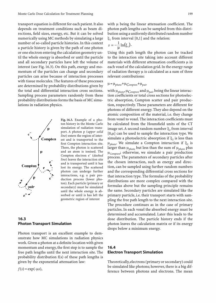
Monte Carlo Dose Calculation for Treatment Planning 199

transport equation is different for each patient. It also depends on treatment conditions such as beam di-rections, fi eld sizes, energy, etc. But it can be solved numerically using MC methods by simulating a large number of so-called particle histories. In this context a particle history is given by the path of one photon or one electron entering the calculation geometry un-til the whole energy is absorbed or until the particle and all secondary particles have left the volume of interest (see Fig. 16.3). On this path, energy and mo-mentum of the particles can change and secondary particles can arise because of interaction processes with tissue molecules. The features of these processes are determined by probability distributions given by the total and differential interaction cross sections. Sampling process parameters randomly from these probability distributions forms the basis of MC simu-lations in radiation physics.

with being the linear attenuation coeffi cient. The photon path lengths can be sampled from this distri-bution using a uniformly distributed random number

1 from interval [0,1] and the relation:

( )ln11ξµ−=s .

Using this path length the photon can be tracked to the interaction site taking into account different materials with different attenuation coeffi cients in each voxel of the calculation grid. In the energy range of radiation therapy is calculated as a sum of three relevant contributions:

= photo+ Compton+ pair

with photo, Compton and pair being the linear interac-tion coeffi cients or total cross sections for photoelec-tric absorption, Compton scatter and pair produc-tion, respectively. These parameters are different for photons of different energy. They also depend on the atomic composition of the material, i.e. they change from voxel to voxel. The interaction coeffi cients must be calculated from the Hounsfi eld units of the CT image set. A second random number 2 from interval [0, ] can be used to sample the interaction type. We simulate a photoelectric absorption if 2 is less than

photo. We simulate a Compton interaction if 2 is larger than photo but less than the sum of photo plus

Compton; otherwise, we simulate a pair production process. The parameters of secondary particles after the chosen interaction, such as energy and direc-tion, can be sampled using further random numbers and the corresponding differential cross sections for that interaction type. The formulas of the probability distributions are more complex compared with the formulas above but the sampling principle remains the same. Secondary particles are simulated like the primary particle, i.e. their transport starts with sam-pling the free path length to the next interaction site. The procedure continues as in the case of primary particles. In each voxel the absorbed energy must be determined and accumulated. Later this leads to the dose distribution. The particle history ends if the photon leaves the calculation matrix or if its energy drops below a minimum energy.

16.4 Electron Transport Simulation

Theoretically, electrons (primary or secondary) could be simulated like photons; however, there is a big dif-ference between photons and electrons. The mean

Fig. 16.3. Example of a pho-ton history in the Monte Carlo simulation of radiation trans-port. A photon p (upper solid line) enters the region of inter-est and is transported to the fi rst Compton interaction site. There, the photon is scattered and an atom is ionised. The Compton electron e- (dashed line) leaves the interaction site and is transported until it has lost its energy. The scattered photon can undergo further interactions, e.g. a pair pro-duction process (lower pho-ton). Each particle (primary or secondary) must be simulated until the whole energy is ab-sorbed or until is has left the geometric region of interest

16.3 Photon Transport Simulation

Photon transport is an excellent example to dem-onstrate how MC simulations in radiation physics work. Given a photon at a defi nite location with given momentum and energy, the fi rst step is to sample the free path lengths until the next interaction site. The probability distribution f(s) of these path lengths is given by the exponential attenuation law:

ƒ(s) = exp(- s),

200 M. Fippel

free path lengths of photons between two interaction sites in human tissue is of the order of several centi-metres; therefore, the procedure described in section 16.3 works very well. Electrons, on the other hand, undergo millions of interaction processes along their path through the patient; therefore it would be too time-consuming to simulate electrons like pho-tons. Fortunately, most of the electron interactions are elastic or semi-elastic, i.e. without or with small transfer of energy; therefore, electron interactions can be classifi ed into two groups: hard interactions with large energy transfer and soft collisions without or with small electron energy loss. Hard interactions can be simulated explicitly, and soft collisions can be simulated by continuous electron energy transfer to the surrounding tissue. This technique, called con-densed history technique, was introduced by Berger (1963). Direction changes of the electron due to elas-tic collisions are modelled using a multiple scattering theory; therefore the multiple scattering properties of the different media must be known. Also the electron stopping power is an important material parameter to calculate the correct amount of energy transferred from the electron to the medium. The electron stops if its residual range becomes smaller than the voxel size or the spatial resolution.

To classify electron interactions into hard interac-tions and soft collisions, an arbitrary parameter must be introduced. Typically this parameter is given by a threshold energy. The collision is called soft if the en-ergy transfer in a collision is smaller than this thresh-old energy; otherwise, it is called hard. During hard interactions, secondary electrons (also called delta electrons) or “bremsstrahlung” photons can be re-leased. In a Monte Carlo calculation these secondary particles are simulated like primary particles, again with the capability to emit further secondary par-ticles. Because the threshold energy is an arbitrary parameter, the fi nal result, e.g. the dose distribution, must not depend on the value of this parameter.

There are additional arbitrary parameters. One of the most important of these parameters is the maxi-mum length of a condensed history step. This param-eter is necessary to minimize the error introduced by the condensed history technique. The path of electrons between two hard interactions in condensed history simulations is modelled by a straight line. This is in contradiction to nature, because electron paths are curved; therefore, the charged particle path length (or range) can be overestimated in the simulation. Most Monte Carlo algorithms calculate path length cor-rections to avoid this overestimation. Nevertheless, the simulation results can be wrong, if the electron

path length is too large. A further problem of the con-densed history technique arises if the electron crosses a boundary of different media. Also here artefacts can be avoided by restricting the length of the condensed electron steps; therefore, the maximum step length must not be too large. On the other hand, it should not be too small. In this case the simulation time can be too long. Meanwhile there are sophisticated con-densed history algorithms (Kawrakow 2000a) with almost no artefacts. With these algorithms step-size restrictions are no longer necessary.

The discussion of these problems is included here to show that the use of Monte Carlo techniques with-out care is no guarantee for correctness. It also shows that Monte Carlo is not absolutely equivalent to na-ture. There are a lot of potential sources for errors. But on the other hand, only Monte Carlo algorithms have the potential to be as accurate as possible. This is not the case for all other types of dose calculation.

16.5 Statistical Noise and Variance Reduction Techniques

The statistical variance or noise in each voxel is deter-mined by the number of simulated particle histories. The more histories are simulated, the smaller is the statistical variance. The number of histories must be increased by a factor of four to reduce the statistical variance by a factor of two, i.e. the calculation time in-creases by a factor of four. For an accurate dose distri-bution the statistical variance should be smaller than 2% relative to the maximum dose of the distribution. This accuracy can be achieved by simulating a cor-responding number of histories; however, this may lead to long calculation times. Often, this time is not available in clinical practise; therefore, other tech-niques and tricks are required to reduce the variance. These variance reduction techniques do not require additional computer time. During past years many such techniques have been developed and tested such as interaction forcing, cross-section enhancement, woodcock tracing, initial-ray tracing, particle split-ting, Russian roulette, correlated sampling the use of quasi-random numbers, history repetition, continu-ous boundary crossing, range rejection, and Super Monte Carlo or Macro Monte Carlo (Kawrakow and Fippel 2000). Furthermore, approximations can be implemented to reduce the variance. Examples are the Kerma approximation for photons with an energy smaller than a cut-off value or the continu-

Monte Carlo Dose Calculation for Treatment Planning 201

ous slowing approximation for electrons below some minimum energy. All the additional parameters must be chosen carefully to assure correct results within the allowed accuracy limitations.

Another possibility to reduce the variance are de-noising techniques and fi lters. These techniques are known from diagnostic imaging. During the image measurement process the detector signal is super-imposed by noise. This noise can be removed using digital fi lters. Similar techniques can also be used to smooth a MC-generated 3D dose distribution. Known techniques are, for example, Savitzky-Golay fi lters (Kawrakow 2002), wavelet threshold denois-ing (Deasy et al. 2002), anisotropic diffusion (Miao et. al 2003) and iterative reduction of noise methods (Fippel and Nüsslin 2003); however, there is a prob-lem with all these methods: they can introduce sys-tematic bias and the amount of this systematic error is diffi cult to estimate. Therefore, these techniques should be used with care. They should be part of a MC treatment planning system. They can shorten the planning time especially in the intermediate stage of the planning process; however, the fi nal clinical deci-sion should not be based on smoothed dose distribu-tions, i.e. after the plan optimisation, the whole dose distribution should be recomputed without denois-ing fi lters.

Unfortunately, it is impossible to remove all sta-tistical fl uctuations from the dose distributions, be-cause it is impossible to simulate an infi nite number of histories. In an isodose line representation of the dose distribution this may lead to jagged isodose lines (see Fig. 16.4). This can be problematic because it is not clear in advance whether this is caused just by noise or by a real physical effect; therefore, we have to learn how to deal with these fl uctuations. Generally, in air the statistical variance is larger compared with soft tissue; thus, we can assume a jagged isoline in air is probably caused just by noise (Fig. 16.4).

The Monte Carlo simulation time also depends on parameters such as energy, fi eld size and voxel size. Increasing the energy in the case of electron beams leads to larger ranges of the electrons; therefore, more time for tracing these electrons is required. In the case of photon beams the calculation time only slightly depends on the nominal energy. If we in-crease the fi eld size, more particle histories must be simulated, i.e. the calculation time is approximately proportional to the fi eld area for both, electron and photon beams. Also the voxel size is a sensitive pa-rameter to control the calculation speed. With larger voxels the simulation can be accelerated considerably. On the other hand, spatial resolution is lost. For the

intermediate planning stage larger voxels can be very useful. The fi nal dose distribution should be calcu-lated with high spatial precision; therefore, the plan-ning system should permit the change of voxel sizes.

16.6 Material Parameters

For an accurate simulation of photon and electron transport through human tissue the interaction cross sections must be known. For photons we have to know mainly the interaction coeffi cients for photo-electric absorption, Compton scatter and pair pro-duction. For electrons we have to know the collision and radiation stopping powers as well as the scat-tering power in each voxel. These parameters can be calculated if the atomic composition is known; however, in general we only know the CT number for the corresponding volume element.

In a straight forward approach it is possible to divide the whole range of CT numbers (Hounsfi eld units) into intervals with each interval corresponding to a defi nite material or tissue type. For these materi-als the cross sections can be calculated and tabulated taking into account their atomic composition; thus, the cross sections can be determined in each voxel based on the CT number information. A major prob-lem of this approach is that a large cross-section data basis for each material is needed. If the number of materials is too small, the errors can be signifi cant.

Fig. 16.4. Dose distribution calculated with Monte Carlo for an IMRT patient (head and neck case). The treatment plan consists of 94 multi-leaf collimator segments. The patient was irradiated with 6-mV photon beams of seven different direc-tions. The dose in air is also calculated

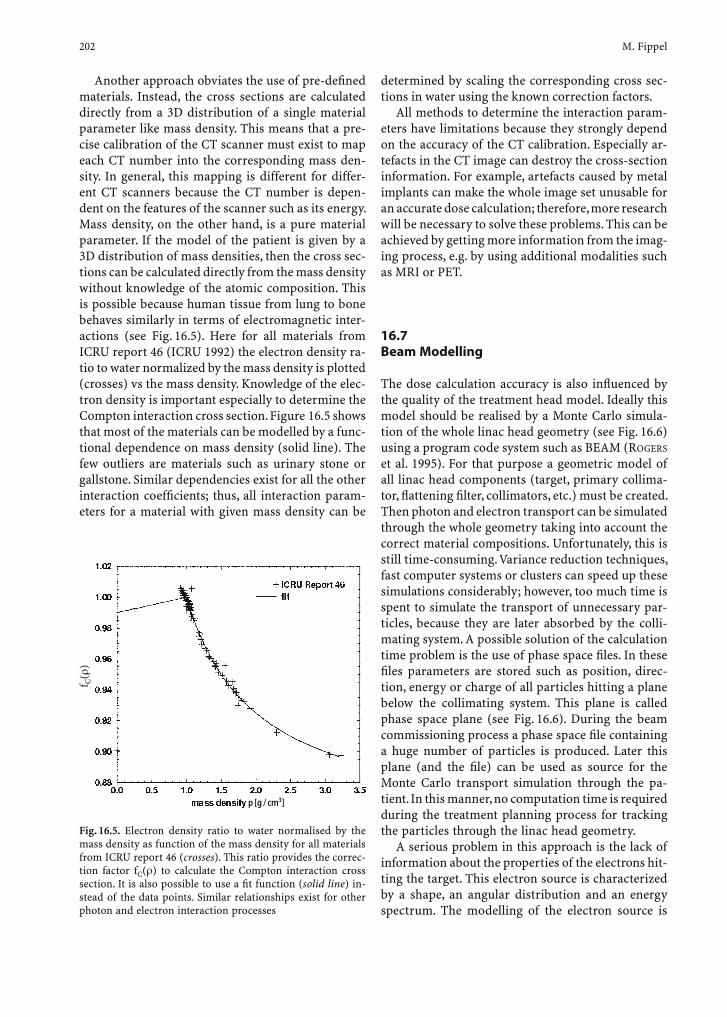
202 M. Fippel

Another approach obviates the use of pre-defi ned materials. Instead, the cross sections are calculated directly from a 3D distribution of a single material parameter like mass density. This means that a pre-cise calibration of the CT scanner must exist to map each CT number into the corresponding mass den-sity. In general, this mapping is different for differ-ent CT scanners because the CT number is depen-dent on the features of the scanner such as its energy. Mass density, on the other hand, is a pure material parameter. If the model of the patient is given by a 3D distribution of mass densities, then the cross sec-tions can be calculated directly from the mass density without knowledge of the atomic composition. This is possible because human tissue from lung to bone behaves similarly in terms of electromagnetic inter-actions (see Fig. 16.5). Here for all materials from ICRU report 46 (ICRU 1992) the electron density ra-tio to water normalized by the mass density is plotted (crosses) vs the mass density. Knowledge of the elec-tron density is important especially to determine the Compton interaction cross section. Figure 16.5 shows that most of the materials can be modelled by a func-tional dependence on mass density (solid line). The few outliers are materials such as urinary stone or gallstone. Similar dependencies exist for all the other interaction coeffi cients; thus, all interaction param-eters for a material with given mass density can be

determined by scaling the corresponding cross sec-tions in water using the known correction factors.

All methods to determine the interaction param-eters have limitations because they strongly depend on the accuracy of the CT calibration. Especially ar-tefacts in the CT image can destroy the cross-section information. For example, artefacts caused by metal implants can make the whole image set unusable for an accurate dose calculation; therefore, more research will be necessary to solve these problems. This can be achieved by getting more information from the imag-ing process, e.g. by using additional modalities such as MRI or PET.

16.7 Beam Modelling

The dose calculation accuracy is also infl uenced by the quality of the treatment head model. Ideally this model should be realised by a Monte Carlo simula-tion of the whole linac head geometry (see Fig. 16.6) using a program code system such as BEAM (ROGERS et al. 1995). For that purpose a geometric model of all linac head components (target, primary collima-tor, fl attening fi lter, collimators, etc.) must be created. Then photon and electron transport can be simulated through the whole geometry taking into account the correct material compositions. Unfortunately, this is still time-consuming. Variance reduction techniques, fast computer systems or clusters can speed up these simulations considerably; however, too much time is spent to simulate the transport of unnecessary par-ticles, because they are later absorbed by the colli-mating system. A possible solution of the calculation time problem is the use of phase space fi les. In these fi les parameters are stored such as position, direc-tion, energy or charge of all particles hitting a plane below the collimating system. This plane is called phase space plane (see Fig. 16.6). During the beam commissioning process a phase space fi le containing a huge number of particles is produced. Later this plane (and the fi le) can be used as source for the Monte Carlo transport simulation through the pa-tient. In this manner, no computation time is required during the treatment planning process for tracking the particles through the linac head geometry.

A serious problem in this approach is the lack of information about the properties of the electrons hit-ting the target. This electron source is characterized by a shape, an angular distribution and an energy spectrum. The modelling of the electron source is

p [g / cm3]

Fig. 16.5. Electron density ratio to water normalised by the mass density as function of the mass density for all materials from ICRU report 46 (crosses). This ratio provides the correc-tion factor fC( ) to calculate the Compton interaction cross section. It is also possible to use a fi t function (solid line) in-stead of the data points. Similar relationships exist for other photon and electron interaction processes

f C(

)

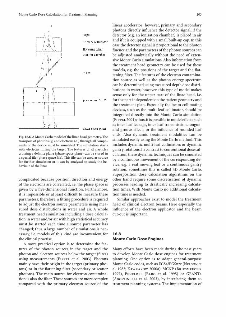
Monte Carlo Dose Calculation for Treatment Planning 203

complicated because position, direction and energy of the electrons are correlated, i.e. the phase space is given by a fi ve-dimensional function. Furthermore, it is impossible or at least diffi cult to measure these parameters; therefore, a fi tting procedure is required to adjust the electron source parameters using mea-sured dose distributions in water and air. A whole treatment head simulation including a dose calcula-tion in water and/or air with high statistical accuracy must be started each time a source parameter has changed; thus, a large number of simulations is nec-essary, i.e. models of this kind are inconvenient for the clinical practise.

A more practical option is to determine the fea-tures of the photon sources in the target and the photon and electron sources below the target (fi lter) using measurements (Fippel et al. 2003). Photons mainly have their origin in the target (primary pho-tons) or in the fl attening fi lter (secondary or scatter photons). The main source for electron contamina-tion is also the fi lter. These sources are more complex compared with the primary electron source of the

linear accelerator; however, primary and secondary photons directly infl uence the detector signal, if the detector (e.g. an ionisation chamber) is placed in air and if it is equipped with a small built-up cap. In this case the detector signal is proportional to the photon fl uence and the parameters of the photon sources can be adjusted analytically without the need of exten-sive Monte Carlo simulations. Also information from the treatment head geometry can be used for these models, e.g. the positions of the target and the fl at-tening fi lter. The features of the electron contamina-tion source as well as the photon energy spectrum can be determined using measured depth dose distri-butions in water; however, this type of model makes sense only for the upper part of the linac head, i.e. for the part independent on the patient geometry and the treatment plan. Especially the beam collimating devices, such as the multi-leaf collimator, should be integrated directly into the Monte Carlo simulation (Fippel 2004); thus, it is possible to model effects such as inter-leaf leakage, inter-leaf transmission, tongue-and-groove effects or the infl uence of rounded leaf ends. Also dynamic treatment modalities can be simulated easily using the Monte Carlo method. This includes dynamic multi-leaf collimators or dynamic gantry rotations. In contrast to conventional dose cal-culation, these dynamic techniques can be simulated by a continuous movement of the corresponding de-vice, e.g. a real moving leaf or a continuous gantry rotation. Sometimes this is called 4D Monte Carlo. Superposition dose calculation algorithms on the other hand require some discretisation of dynamic processes leading to drastically increasing calcula-tion times. With Monte Carlo no additional calcula-tion time is needed.

Similar approaches exist to model the treatment head of clinical electron beams. Here especially the infl uence of the electron applicator and the beam cut-out is important.

16.8 Monte Carlo Dose Engines

Many efforts have been made during the past years to develop Monte Carlo dose engines for treatment planning. One option is to adapt general-purpose Monte Carlo codes, such as EGS4/EGSnrc (Nelson et al. 1985; Kawrakow 2000a), MCNP (Briesmeister 1997), Penelope (Baro et al. 1995) or GEANT4 (Agostinelli et al. 2003), by interfacing them to treatment planning systems. The implementation of

Fig. 16.6. A Monte Carlo model of the linac head geometry. The transport of photons ( ) and electrons (e-) through all compo-nents of the device must be simulated. The simulation starts with electrons hitting the target. The features of all particles crossing a defi nite plane (phase space plane) can be stored in a special fi le (phase space fi le). This fi le can be used as source for further simulation or it can be analysed to study the be-haviour of the linac

204 M. Fippel

additional variance reduction techniques (see sec-tion 16.5) leads to calculation times acceptable for clinical routine. Examples of this approach are the Macro Monte Carlo code (Neuenschwander and Born 1992) for electron beams as well as the Super Monte Carlo technique (Keall and Hoban 1996) and MCDOSE (Ma et al. 2002), both for photon and electron beams. A second option is the development of entirely new Monte Carlo codes especially de-signed for radiotherapy purposes. Examples are the Voxel Monte Carlo (VMC) algorithm (Kawrakow et al. 1996) for electron beams, its extensions for photon beams XVMC (Fippel 1999) and VMC++ (Kawrakow 2000b), the DPM code (Sempau et al. 2000) and the PEREGRINE system (Hartmann Siantar et al. 2001).

These new techniques allow dose calculations within minutes for photon beams and within sec-onds for electron beams using computer clusters (e.g. PEREGRINE) or ordinary personal computers (XVMC, VMC++). All treatment planning companies are working on the implementation of Monte Carlo for dose calculation. Some systems are already avail-able. In the future all conventional dose algorithms will be replaced by Monte Carlo.

16.9 Monte Carlo Dose Calculation for Inverse Planning and IMRT

The quality of dose calculation is of special impor-tance for inverse treatment planning (see Chap. 17) in IMRT (see Chap. 24). In contrast to conventional ra-diotherapy, with IMRT techniques larger dose values can be achieved in the tumour volume compared with the organs at risk. This leads to large dose gradients if these organs are close to the tumour. The situation is even more complex if these structures are located in an environment with density inhomogeneities con-sisting of soft tissue, bone and air cavities. This is the case especially in the head, neck and thorax regions. Here the infl uence of photon Compton scatter and lateral electron fl ow is not negligible. Conventional dose calculation algorithms (see Chap. 15) often fail to predict the dose in the neighbourhood of air cavi-ties. The effect of secondary electron transport is energy dependent. For small energies (like 6 mV) the range of these electrons is of the order of 1 cm in water. For large energies (15 or 18 mV) this range is larger (up to 5 cm); therefore, dose errors can be large if the secondary electron transport is not modelled

correctly. In inverse planning the dose error trans-lates into a corresponding convergence error, i.e. the dose distribution will be as required, but the fl uence distribution is wrong. In other words, the fl uence dis-tribution determined during the optimisation pro-cess will in reality lead to a dose distribution different to the calculation and different to the requirements from the objective function.

A further problem in IMRT arises with the mod-elling of the beam delivery system, i.e. mainly with the multi-leaf collimator or the compensator. These devices have a signifi cant infl uence on the dose cal-culation (see section 16.7). Many IMRT planning systems optimise photon fl uence weights. The MLC sequences are generated subsequent to the optimisa-tion process. To ensure correct dose distributions a dose re-calculation must be performed based on the generated MLC segments. Often Monte Carlo algo-rithms are used for the purpose of dose verifi cation. A treatment plan re-optimisation may be necessary if the result of the dose verifi cation is signifi cantly dif-ferent from the optimised dose distribution.

A better alternative is the integration of the MLC modelling and sequencing (or the modelling and calculation of Compensator shapes) into the opti-misation loop (Alber et al. 2003). This means that after the optimisation of the fl uence weights the MLC sequencing process is started. Then the dose dis-tribution for each MLC segment can be calculated separately using Monte Carlo taking into account full head scatter, MLC leakage, MLC transmission and tongue-and-groove effects. Now the optimisation process is initiated again with the aim to improve the total dose distribution by adjusting the weights of each segment. Using this approach it is also pos-sible to change MLC contours, i.e. to change leaf posi-tions. For this purpose the dose distribution for the corresponding segment must be re-calculated. In this manner there is no disagreement between the opti-mised dose distribution and the fi nal calculated dose distribution.

A real clinical benefi t from Monte Carlo can be expected if it is used in conjunction with IMRT and inverse planning. On the other hand, there are addi-tional problems in inverse planning if we use Monte Carlo for dose calculation instead of analytical tech-niques. One problem is caused by the statistical noise. It has been shown theoretically (Kawrakow 2004) that the statistical uncertainty of the dose in each voxel causes a systematic uncertainty of the objec-tive function. Fortunately, this systematic deviation can be calculated and taken into account during the optimisation. Another problem comes from the ran-

Monte Carlo Dose Calculation for Treatment Planning 205

dom number generator. The fi nal dose distribution changes slightly if we change the initial state (also called seed) of the random number generator. But this can lead to different solutions of the optimisa-tion problem if the objective function provides a large variety of optimum treatment plans. In this case we have to accept that there is more than one reasonable result. A third problem can arise from voxels of air belonging to the planning target volume. Generally, this is no problem for conventional dose calculation such as pencil-beam dose calculation because these algorithms have the tendency to overestimate the dose in air. Using Monte Carlo the dose in air is cal-culated correctly, i.e. it is signifi cantly smaller than the dose in the surrounding tissue. If these voxels are part of the target volume, the optimisation algorithm tries to compensate for this apparent underdoseage. However, clinically this compensation is unnecessary; therefore, we should avoid air in the planning target volume wherever possible. This may be diffi cult if the planning target volume is given by the clinical tar-get volume with a margin to take into account setup and motion errors. It will be impossible to avoid air in the planning target volume if air cavities are close to the clinical target volume. In these cases it is useful to introduce weight factors with small weights in the objective function for regions with air in the target volume.

16.10 Monte Carlo Dose Calculation for Ion Beam Therapy

The electromagnetic interaction properties of pro-tons and heavier ions are similar to electrons; how-ever, because of their larger mass, ions show less lat-eral scattering effects. Only in the Bragg-Peak region is the beam broadened because of multiple elastic scattering; therefore, dose calculation can be per-formed accurately and effi ciently using pencil-beam algorithms. On the other hand, nuclear interaction processes have a signifi cant infl uence on dose and radio-biological effectiveness. Within the framework of pencil beam dose calculation these process can be taken into account only in an approximate manner. Especially the dependence of the nuclear interaction cross sections on the tissue composition is diffi cult to model. Using Monte Carlo this is much easier and more precise. The most important requirements are accurate cross sections and nuclear interaction mod-els. If this is available, all kinds of particles produced

in nuclear reactions can be simulated and tracked through the patient anatomy in a manner similar to electrons and photons.

References

Agostinelli S et al. (2003) GEANT4–a simulation toolkit. Nucl Instrum Methods A506:250–303

Alber M, Birkner M, Bakai A, Dohm O, Fippel M, Paulsen F, Belka C, Budach W, Nüsslin F (2003) Routine use of Monte Carlo dose computation for head and neck IMRT optimiza-tion. Int J Radiat Oncol Biol Phys 57 (Suppl) 1:S208

Baro J, Sempau J, Fernandez-Varea JM, Salvat F (1995) PENEL-OPE: an algorithm for Monte Carlo simulation of the pen-etration and energy loss of electrons and positrons in matter. Nucl Instrum Methods B100:31–46

Berger MJ (1963) Monte Carlo Calculation of the penetration and diffusion of fast charged particles. In: Alder B, Fern-bach S, Rotenberg M (eds) Methods in computational phys-ics. Academic Press, New York, pp 135–215

Briesmeister JF (1997) MCNP – a general Monte Carlo N-Particle Transport Code. Los Alamos National Laboratory Report No. LA-12625-M

Deasy JO, Wickerhauser V, Picard M (2002) Accelerating Monte-Carlo simulations of radiation therapy dose dis-tributions using wavelet threshold denoising. Med Phys 29:2366–2377

Fippel M (1999) Fast Monte Carlo dose calculation for photon beams based on the VMC electron algorithm. Med Phys 26:1466–1475

Fippel M (2004) Effi cient particle transport simulation through beam modulating devices for Monte Carlo treatment plan-ning. Med Phys 31:1235–1242

Fippel M, Nüsslin F (2003) Smoothing MC calculated dose dis-tributions by iterative reduction of noise. Phys Med Biol 48:1289–1304

Fippel M, Haryanto F, Dohm O, Nüsslin F, Kriesen S (2003) A virtual photon energy fl uence model for Monte Carlo dose calculation. Med Phys 30:301–311

Hartmann Siantar CL, Walling RS, Daly TP, Faddegon B, Albright N, Bergstrom P, Chuang C, Garrett D, House RK, Knapp D, Wieczorek DJ, Verhey LJ (2001) Description and dosimetric verifi cation of the PEREGRINE Monte Carlo dose calculation system for photon beams incident on a water phantom. Med Phys 28:1322–1337

ICRU (1992) Photon, electron and neutron interaction data for body tissues. International Commission on Radiation Units and Measurements (ICRU), Report 46

Kawrakow I (2000a) Accurate condensed history Monte Carlo simulation of electron transport, I. EGSnrc, the new EGS4 version. Med Phys 27:485–498

Kawrakow I (2000b) VMC++, electron and photon Monte Carlo calculations optimized for radiation treatment plan-ning. In: Proc MC2000 Conference, Lisbon. Springer, Berlin Heidelberg New York, pp 229–236

Kawrakow I (2002) On the denoising of MC calculated dose distribution. Phys Med Biol 47:3087–3103

Kawrakow I (2004) The effect of Monte Carlo statistical uncer-tainties on the evaluation of dose distributions in radiation treatment planning. Phys Med Biol 49:1549–1556

206 M. Fippel

Kawrakow I, Fippel M (2000) Investigation of variance reduc-tion techniques for Monte Carlo photon dose calculation using XVMC. Phys Med Biol 45:2163–2183

Kawrakow I, Fippel M, Friedrich K (1996) 3D electron dose calculation using a voxel-based Monte Carlo algorithm (VMC). Med Phys 23:445–457

Keall PJ, Hoban PW (1996) An accurate 3-D X-ray dose calcu-lation method combining superposition and pre-generated Monte-Carlo electron track histories. Med Phys 23:479–485

Ma CM, Li JS, Pawlicki T, Jiang SB, Deng J, Lee MC, Koumrian T, Luxton M, Brain S (2002) A Monte Carlo dose calcula-tion tool for radiotherapy treatment planning. Phys Med Biol 47:1671–1689

Miao B, Jeraj R, Bao S, Mackie T (2003) Adaptive anisotropic

diffusion fi ltering of MC dose distributions. Phys Med Biol 48:2767–2781

Nelson WR, Hirayama H, Rogers DWO (1985) The EGS4 Code System. SLAC Report No. SLAC-265

Neuenschwander H, Born E (1992) A macro Monte Carlo method for electron beam dose calculations. Phys Med Biol 37:107–125

Rogers DWO, Faddegon BA, Ding GX, Ma CM, Wei J, Mackie TR (1995) BEAM: a Monte Carlo code to simulate radio-therapy treatment units. Med Phys 22:503–524

Sempau J, Wilderman SJ, Bielajew AF (2000) DPM, a fast, accu-rate Monte Carlo code optimized for photon and electron radiotherapy treatment planning dose calculations. Phys Med Biol 45:2263–2291

Optimization of Treatment Plans, Inverse Planning 207

17 Optimization of Treatment Plans, Inverse Planning

Thomas Bortfeld and Christian Thieke

T. Bortfeld, PhDDepartment of Radiation Oncology, Massachusetts General Hospital, 30 Fruit Street, Boston, MA 02114, USAC. Thieke, MD, PhDDepartment of Radiation Oncology, German Cancer Research Center (DKFZ), Im Neuenheimer Feld 280, 69120 Heidelberg, Germany

17.1 Introduction

Computerized optimization of treatment plans has been proposed in radiation therapy since comput-ers became available to hospitals in the 1960s (Hope et al. 1967; Bahr et al. 1968; Redpath et al. 1975; McDonald and Rubin 1977). The fi rst prototypes were presented at that time but did not fi nd their way into clinical practice. The main reason was that those early approaches were basically restricted to the optimization of beam weights, sometimes in com-bination with wedges, which have a limited potential

to shape dose distributions in 3D. Optimization of beam directions in fully 3D was not really possible with computers of that time.

The situation changed drastically with the inven-tion of intensity-modulated radiation therapy (see Chap. 23) by Brahme and colleagues in 1982, along with exponential increase of computer power. The IMRT has a much greater potential to shape complex spatial dose distributions. Interestingly, the fi rst ap-proaches to calculate intensity maps for IMRT were not based on optimization techniques. They instead inverted the underlying integral equation analyti-cally, which means that the spatial dose distribution was prescribed, and the beam intensity distribution that would precisely yield this dose distribution was calculated. To fi nd an exact solution to this inverse problem, several assumptions and approximations had to be made, and solutions could only be found for very simple symmetrical cases. Nevertheless, based on this inversion idea, IMRT planning is often still called inverse planning. Other early attempts at solv-ing the inverse problem of radiation therapy plan-ning used deconvolution techniques that were bor-rowed from image processing (Brahme et al. 1982; Holmes et al. 1991). Again, the solutions were always approximations.

A true solution of the inverse problem cannot be found in any but the simplest hypothetical cases, because the beam intensities can never become negative and therefore we can never subtract dose. Mathematically, the problem to generate a desired dose distribution with rays of radiation of variable intensity is equivalent to the problem of creating an arbitrary drawing using uniform straight lines drawn with a pencil and ruler on paper. This problem was mathematically analyzed by Birkhoff (1940). He found that the problem can only be solved if an eraser is also available. Unfortunately, we do not have a physical dose eraser at hand in radiation therapy.

Therefore, other mathematical methods were soon applied to this problem. One of them is called feasi-bility search (Censor et al. 1988; Starkschall et al. 2000). Here the idea is that, even though there is no

CONTENTS

17.1 Introduction 20717.2 Optimization Principles 20817.2.1 Optimization Criteria 20817.2.1.1 Physical Dose Criteria 20917.2.1.2 Physical and Technical IMRT Delivery Criteria 21017.2.1.3 The Objective Function 21017.2.2 Variables to Be Optimized 21117.2.2.1 Intensity Maps 21117.2.2.2 Number of Beams 21117.2.2.3 Beam Angles 21217.2.2.4 Number of Intensity Levels 21217.2.2.5 Beam Energy 21217.2.3 Optimization Algorithms 21217.3 Inverse Planning in Practice 21317.3.1 General Approach 21317.3.2 Clinical Example 21517.4 Multicriteria Optimization in Inverse Planning 21617.5 Conclusion 218 References 218

208 T. Bortfeld and C. Thieke

exact solution to the inverse problem that will yield the ideal dose distribution to the tumor with no dose to normal structures, we may still be able to fi nd a plan that fulfi lls all clinical and physical constraints. This approach can be very useful if the constraints are carefully chosen: we do not want to make it too easy to fulfi ll the constraints because that may result in suboptimal plans. We also do not want to over-constrain the problem, because then there will be no solution at all. Feasibility search could be particularly successful for clinical cases that do not vary too much between individuals, such as prostate cancer. Here it is possible to fi nd class solutions of constraints that will yield good treatment plans for many patients.

Presently, the most commonly used approach in IMRT planning is the optimization approach, in which one tries to fi nd the best physically and tech-nically possible treatment plan with respect to given physical and clinical criteria. Among the fi rst pub-lished optimization techniques were those by Webb (1989) and Bortfeld et al. (1990). It was shown that with the optimization approach complex dose dis-tributions could be generated with a limited num-ber (less than ten) of beam directions (Bortfeld et al. 1990). In most other previous approaches the use of an unrealistically large number of beams was assumed. This paved the way for implementation of IMRT at conventional linear accelerators equipped with a multileaf collimator. Even though we focus on IMRT optimization, many of the concepts that we dis-cuss in this chapter can be applied to general radio-therapy optimization with other modalities.

We fi rst discuss the principles of current optimiza-tion approaches in IMRT. In section 3 we discuss the clinical aspects of IMRT optimization, and in section 4 we give an outlook on future developments in this fi eld.

17.2 Optimization Principles

Optimization is mathematically defi ned as the maxi-mization or minimization of a score (a number) un-der certain constraints. The scoring function (also called “objective function”), which yields the score, is a function of all variables that need to be optimized. In general mathematical optimization the problem is to fi nd the set of variables that yield the maximum (or minimum) score while fulfi lling all constraints. Specifi cally, in radiotherapy optimization the prob-lem is to fi nd the treatment plan with all its associated

variables (e.g., beam intensities and angles) that yield the best scoring treatment for an individual patient. In IMRT the number of variables (the intensities for all beam elements for all beams) can be in the thousands, so we are typically dealing with a highly dimensional optimization problem; however, it is im-portant to note that the score is a single number. The issues that are related with this are discussed later, but it is immediately clear that it is a formidable task to characterize the goodness of a radiation treatment plan with a single number.

The basics of optimization in radiotherapy have been discussed in many recent reviews and book chapters (Bortfeld 1999; IMRT 2001; Bortfeld 2003; Censor 2003), so we are brief on this subject.

17.2.1 Optimization Criteria

The defi nition of the objective function and con-straints (for which we use the combined term “op-timization criteria” in the sequel) is arguably the most challenging part of IMRT optimization, and requires a lot of thought. Optimization criteria that are not clinically relevant or not complete can lead to treatment plans that are mathematically optimal but clinically useless. Mathematical optimality is not a guarantee for a good treatment plan at all. In the defi -nition of the objective function one has to translate the clinical experience gained over the past 100 years or so into mathematical terms, which in turn needs to be translated into computer language. The key ques-tion is: What characterizes the “best” treatment plan? Clinicians often fi nd it diffi cult to formulate a com-plete, unique, quantitative set of optimization (scor-ing) criteria for radiotherapy planning, even though they feel capable of ranking individually prepared plans (Langer et al. 2003). This is somewhat differ-ent from other applications of optimization, e.g., in economics, in which the objective is often quite clear (e.g., minimize the cost).

It may seem obvious to defi ne the optimization criteria in terms of treatment outcome, say, maxi-mize the probability of curing the patient without exceeding tolerance limits of side effects in normal tissues. The problem is that there exists no commonly accepted and validated model that translates the physical dose distribution into normal tissue compli-cation probabilities (NTCP) or tumor control prob-abilities (TCP), let alone cure rates. In 1968 Alexander Solzhenitsyn wrote in his novel Cancer Ward: “There was no formula for calculating the right intensity of

Optimization of Treatment Plans, Inverse Planning 209

dose, for knowing how much would be most lethal for an individual tumor yet least harmful to the rest of the body.” Even though many clinical studies have been performed since then, and a lot of data has been collected, this basic problem still persists.

The most common approach in practical radio-therapy optimization at present is therefore to use optimization criteria that are defi ned in terms of the physical dose distribution. In many cases these criteria are not absolutely fi xed, but are adjusted by the treatment planner in a “human iteration loop,” as the optimization progresses. The clinical aspects of this are explained in detail in the subsequent section. Suffi ce it to say that optimization using these physical criteria is not expected to yield the best clinical plan in one step. What is more important is that these cri-teria provide good “steerability” of the plan: If, after the fi rst optimization run, the plan is not satisfactory from a clinical point of view, an adjustment of the criteria should allow to steer the plan in the desired direction in a straightforward manner using only a few of the “human iteration loops.”

We now discuss optimization criteria that are used in various commercial IMRT optimization systems. The physical dose criteria discussed below can be used as either constraints or as objectives. In the con-straint formulation one merely requests that the cri-teria stay within certain limits. If they are defi ned as (part of) the “objective function,” the goal is to maxi-mize or minimize these quantities.

17.2.1.1 Physical Dose Criteria

A widely used criterion is the quadratic deviation of the actual dose from a prescribed dose level Dmin (in the target volume) or tolerance dose level Dmax (in both the target volume and critical structures), which is to be minimized. Different weight factors (also called penalty factors or importance factors) can be used for underdose and overdose. The objective func-tion (“costlet”) for a particular organ is then:

F b u D d b w d b Di ii

N

( ) ( ) ( )min max

r r r= −⎡⎣ ⎤⎦ + −⎡⎣ ⎤⎦( )+ +=∑

2 2

1

where u and w are the weight factors for under- and overdose, respectively. di(b

v ) is the dose at voxel i as a

function of the beam element (bixel) intensities and other variables (e.g., beam angles) combined into the argument vector b

v . Dmin and Dmax are the prescribed

minimum and maximum doses that should ideally not be exceeded. Note that Dmin and Dmax are not the minimum and maximum doses of the actual dose dis-

tribution di(bv

). One often sets Dmin=Dmax= prescribed dose in the target volume. In critical structures the fi rst term is omitted by setting u=0 (or equivalently, setting the minimum dose constraint to 0). [x]+stands for x if x>0 and 0 otherwise. This quadratic deviation approach has been criticized because it does not suf-fi ciently penalize dose cold spots in the target volume or hot spots in critical structures. For example, if the dose in the target volume becomes zero in only one voxel, F may still be in an acceptable range, as long as most voxels receive the prescription dose. Higher-order measures of the deviation (such as differences taken to the power of 4, 6, …) have been suggested (Fraass 2002) but are not common in clinical IMRT optimization.

One way to enforce dose homogeneity is to put hard constraints on the actual minimum and maxi-mum dose in the target volume (as opposed to the “soft” deviation approach above). For example, an op-timization constraint might require to keep the target dose within –5% and +7% of the prescription dose, as recommended by the International Commission on Radiation Units and Measurements (ICRU 1993). A possible optimization objective is to maximize the minimum dose value in the target volume (Langer et al. 1996). Maximum dose limitations (but, of course, not minimum dose limitations) make sense in critical structures as well. In structures with a serial orga-nization, such as the spinal cord, the complication is correlated with the maximum dose. For example, in the spinal cord the maximum dose should be limited to, for example, 45 Gy.

The mean dose is a useful descriptor of the dose effect in the target volume as long as deviations from the mean are not too big (Brahme 1984; Levegrun et al. 2001). The mean dose is also a useful clinical parameter in critical structures that are organized in parallel, such as the lung (Kwa et al. 1998). It should be noted, however, that different regions in the lung have different radiation sensitivities. The mean dose overall can therefore only be a very coarse predictor of side effects. It should also be emphasized that dif-ferent kinds of complication can occur in the same organ, e.g., in the lung, such that different criteria may have to be used for one organ in the optimization.

Another common method to represent dose effects in parallel critical structures is to use dose-volume histogram (DVH) constraints (Langer and Leong 1989; Langer et al. 1990; Niemierko 1992; Bortfeld et al. 1997; Spirou and Chui 1998; Gustafsson and Langer 2000), which take into consideration the volume dependence to some degree. The DVH con-straints can be formulated as “no more than Vmax% of

210 T. Bortfeld and C. Thieke

the volume should receive more than a dose of Dmax”. They can be visualized as a barrier with a corner at the point Dmax, Vmax on the DVH plot. The use of mul-tiple DVH constraints may also be indicated in some cases (Carol et al. 1997), and DVH constraints can be used for the target volume as well.

One general advantage of physical criteria, such as dose-volume criteria, is that, because they are simply and clearly defi ned, they can be used easily in clinical protocols. Such IMRT protocols using a combination of various physical dose criteria have been developed and distributed by the Radiation Therapy Oncology Group (RTOG, www.rtog.org). A well-known exam-ple is their protocol 022 for IMRT of oropharyngeal cancer.

A potential mathematical problem with dose-vol-ume constraints is that they are non-convex (Deasy 1997). As a consequence of this, optimization based on DVH constraints may get trapped in local minima; however, it has been shown that this is mainly a theo-retical problem, which seems to be of little relevance in practical optimization (Wu and Mohan 2002; Llacer et al. 2003).

The fi nal physical dose criterion that we discuss is the equivalent uniform dose (EUD). It is defi ned as the uniform dose that would create the same biologi-cal effect in a specifi c organ as the actual non-uni-form dose distribution (Brahme 1984; Niemierko 1997). Because it involves the biological effect, it is often interpreted as a biological rather than physical dose criterion; however, according to a more recent defi nition by Niemierko (1999) the EUD is simply the generalized mean (a-norm) of the physical dose distribution:

EUD = ⋅⎛⎝⎜

⎞⎠⎟

∑v di ia

i

a1/

where vi is the volume of voxel i divided by the total volume of the organ. With this defi nition and with a = 1 the EUD is in fact the mean dose and with a = it equals the maximum dose. Of course, the value of a is organ specifi c. Values between 1 and infi nity represent organs with a mixture between parallel and serial structures. It is interesting to note that the value of a can be derived from the well-known power-law relationship of the tolerance dose TD as a function of the relative treated volume v:

TD v TDvn( ) ( )= 1

.

One fi nds that a = 1/n.For target volumes, the value of a is negative. The

beauty of this approach is its simplicity and general-

ity. All organs can be characterized by just one param-eter. The EUD has recently been implemented into experimental IMRT optimization systems (Thieke et al. 2002; WU et al. 2002). A convenient feature of the EUD is that it is a convex function of the dose distribution, and therefore of the beam intensities, for a 1 and for a 0, i.e., for almost all organs. This facilitates optimization and makes the use of projec-tion onto convex sets (POCS) methods possible (Cho et al. 1998; Thieke et al. 2002).

17.2.1.2 Physical and Technical IMRT Delivery Criteria

The most obvious physical limitation of this type is that the beam intensities must not be allowed to take negative values. This does not require any further discussion.

Another important aspect of optimized treat-ment plans is that they have to be deliverable in an acceptable amount of time. Also, small errors in the delivery should not affect the resulting dose distribu-tion too much, i.e., the plan should be robust. Both of these requirements can be fulfi lled with intensity maps that are smooth. If there are multiple solutions to the optimization problem, which is frequently the case, one should obviously choose the solution with the smoothest (easiest to deliver) intensity maps. If one has the choice between a highly conformal plan with extremely complex intensity maps, and a plan that is almost as good but much easier and safer to deliver, one would probably choose the latter plan. Basically there are two ways to ensure smooth inten-sity maps. First, one can smooth the maps using a fi l-ter. Median fi lters can be used for this purpose (Webb et al. 1998; Kessen et al. 2000). Secondly, one can add a smoothing term to the objective function (Alber and Nüsslin 2000).

17.2.1.3 The Objective Function

The criteria (or “costlets”) mentioned in the previ-ous subsections must somehow be combined to form the total objective function. An alternative is to use only one criterion in the objective function and set all other criteria as constraints. The most common approach is to add some criteria using weight fac-tors that refl ect the importance of the different cri-teria. Multiplication of costlets has also been sug-gested (Fraass 2002). A typical approach is to add the deviations from the dose prescription (tumor) and maximum doses (critical structures) as defi ned

Optimization of Treatment Plans, Inverse Planning 211

in subsection 2.1.1 using organ-specifi c weight fac-tors uk and wk. According to this defi nition the opti-mum treatment is the one with the smallest overall deviation from the prescription. In the plan steering process (the “human iteration loop”) it is not a priori clear by how much to change the weights to achieve the desired effect on the dose distribution. Suitable weight factors have to be determined by trial and error, which can be quite time-consuming and is dis-cussed further below. Some researchers argued that optimized “inverse” IMRT planning is just replacing the conventional manual trial-and-error search to fi nd the best beam parameters by a manual trial-and-er-ror search for suitable weight factors and constraints. While there may be some truth to this statement, it is also true that IMRT allows one to deliver highly con-formal concave dose distributions that are impossible to achieve with conventional 3D techniques.

17.2.2 Variables to Be Optimized

After determining the objective function and the set of constraints, the next question is about the variables to be optimized. Even with the most powerful mod-ern computers it is impossible to optimize all treat-ment parameters (variables). In practice, a subset of the treatment parameters, including, for example, the beam angles, need to be manually pre-selected.

17.2.2.1 Intensity Maps

In IMRT the main variables to be optimized are obvi-ously the intensity maps for each beam. Each beam is typically subdivided into beam elements (bixels) of 5×5 to 10×10 mm2. The intensity (fl uence) for each of the bixels is optimized. The total number of bixels for all beams is typically of the order of 1000–10,000. Because there is no way to deliver intensity-modu-lated photon beams directly with a linac, the intensity maps are then converted to a series of multileaf col-limator (MLC) shapes (segments) in a second almost independent step, which is called leaf sequencing. Of course, there has to be some link between optimi-zation and sequencing. For example, the optimizer must know the leaf width of the MLC and should use that as the bixel size in one dimension. More thor-ough approaches for the consideration of delivery constraints in intensity map optimization have also been suggested (Cho and Marks 2000; Alber and Nüsslin 2001).

Besides the common two-step approach, it has also been suggested to avoid the intermediate step of us-ing intensity maps altogether and directly optimize MLC shapes (apertures) and their weights. This ap-proach has been suggested by DeNeve et al. (1996), among others. The MLC shapes can be determined manually based on the geometry (anatomy) of the problem, or they can be directly optimized together with the weights of the segments. The latter method has recently been published (Shepard et al. 2002). The direct optimization of MLC shapes and weights is mathematically a diffi cult, non-convex problem.

17.2.2.2 Number of Beams

The question of how many intensity-modulated beams should be used is highly relevant for the practi-cal delivery of IMRT. As a consequence of the analogy between image reconstruction in computed tomogra-phy (CT) and inverse radiotherapy planning, the early theoretical approaches to inverse planning assumed a very high number of coplanar beams (Brahme et al. 1982; Cormack and Cormack 1987). Later it was recognized that quite acceptable results can also be achieved with a moderate number of beams. In fact, some publications claim that one generally does not need more than three intensity-modulated beams to obtain results that can hardly be improved any more (Söderström and Brahme 1995). These issues have been discussed frequently in the literature (Brahme 1993; Brahme 1994; Mackie et al. 1994; Mohan and Ling 1995; Mohan and Wang 1996; Söderström and Brahme 1996).

In principle, it is clear that the higher the number of beams, the higher is the dose conformation poten-tial; however, the incremental improvement of the conformity of the total dose distribution diminishes as more beams are added. The real question about the “optimum” number of beams in IMRT is therefore: What is the number of beams beyond which one does not see any practically relevant improvement of the treatment plan? Several authors have found indepen-dently that it is hardly ever necessary to use much more than ten intensity-modulated beams to achieve results that are close to optimum (Bortfeld et al. 1990; Webb 1992; Söderström and Brahme 1995; Stein et al. 1997).

On the other extreme, with a number of beams as small as three or four, the conformity of the result-ing dose distribution is considerably reduced when compared with a plan incorporating ten beams; however, thanks to intensity modulation, it is still

212 T. Bortfeld and C. Thieke

possible to imprint the desired shape on at least one isodose curve, e.g., the 80% isodose. This fi nding is related to image reconstruction of homogeneous ob-jects using only three or four projections (Natterer 1986); hence, in cases where the tolerance of the criti-cal structures is not too low as compared with the required target dose, one may get away with very few intensity-modulated beams (Söderström and Brahme 1995).

17.2.2.3 Beam Angles

The question about the optimum beam angles is re-lated to the number of beams. Clearly, if very many beams (more than ten) are used, they can be placed at evenly spaced angular intervals and there will be no need to optimize beam orientations. Even with a moderate number of beams of the order of seven or nine, one may often use evenly spaced beams without compromising the dose distribution (Bortfeld and Schlegel 1993); however, it has been shown that this is case dependent, and complex cases, such as head and neck, sometimes benefi t from beam ori-entation optimization even for nine or more beams (Pugachev et al. 2001). With very few beams, such as four or less, very careful and time-consuming op-timization of beam orientations is always essential; otherwise, one will not be able to achieve acceptable results.

It should be noted that optimal orientations of intensity-modulated beams are generally different from those of uniform beams: in IMRT it is not gen-erally necessary and often not even advantageous to avoid beam directions through organs at risk, because these can be spared by reducing the intensity for the corresponding rays (Stein et al. 1997). Also, for simi-lar reasons, non-coplanar beams are rarely used in IMRT. Another point worth mentioning is that paral-lel opposed beams should be avoided in IMRT, such that, for evenly spaced beams, the number of beams should be odd. The reason for this is that a parallel opposed beam adds much less beam-shaping poten-tial than a slightly angled beam. Clearly, if the attenu-ation were zero, parallel-opposed beams would be completely useless.

17.2.2.4 Number of Intensity Levels

Most IMRT planning methods assume a continuous modulation of the intensity. Several investigations have shown that promising results can be achieved

with step-like beam profi les as well (Bortfeld et al. 1994; Gustafsson et al. 1994; DeNeve et al. 1996). In fact, using a moderate number of stair steps with fi ve to seven “intensity levels” in each beam profi le, the results are almost as good as with continuous modulation (Keller-Reichenbecher et al. 1998). Consequently, it is not necessary to go to a fully dy-namic treatment mode to perform IMRT with an MLC. The IMRT can instead be realized in a “step-and-shoot” mode, i.e., by the successive delivery of a number of static MLC-shaped beam segments from each direction of incidence. The total number of beam segments or “subfi elds” to be delivered in this way is of the order of 100. Modern treatment machines can deliver such a sequence of subfi elds automatically and quickly. A comparison of the fea-tures of dynamic vs step and shoot IMRT has been published by Chui et al. (2001).

17.2.2.5 Beam Energy

The choice of the beam energy is less critical in IMRT than in conventional radiotherapy. In fact, it was sug-gested that very low energies around 1 MeV or less suffi ce in IMRT. The reason is once again that in IMRT one tends to spread the beams more evenly around the patient, and the depth-dose fall-off is therefore not very relevant.

17.2.3 Optimization Algorithms

The objective function as a function of the variables to be optimized, in combination with the optimiza-tion constraints, defi nes the optimization problem. As for its solution, many mathematical algorithms have been developed to solve optimization problems of various kinds. The algorithm of choice depends on the type of the problem (linear/non-linear, convex/non-convex). We cannot describe these algorithms in any detail in this chapter. The interested reader is referred to other reviews (Bortfeld 1999; Shepard et al. 1999).

The most common approach in commercial IMRT optimization systems is the non-linear (often qua-dratic) problem formulation. The algorithm used for fi nding the solution is usually a variant of the “gradi-ent” technique. It converges rapidly and can be ap-plied to a wide range of optimization problems; how-ever, in the non-linear case one does not usually let the algorithm converge to the numerical optimum,

Optimization of Treatment Plans, Inverse Planning 213

but stops after an acceptable number of iteration steps. Statements about the proximity to the true op-timal solution are more diffi cult to make than in the linear case, or impossible.

There is no doubt that in general optimization the biggest experience exists in the fi eld of linear opti-mization algorithms (“linear programming”). Even though many of the IMRT objectives and constraints discussed above are non-linear, a linear model or its variants can approximate the problem suffi ciently well to yield useful solutions (Langer et al. 1996; Romeijn et al. 2003). An advantage of the linear prob-lem formulation is that the optimality of the solution can be proven.

17.3 Inverse Planning in Practice

17.3.1 General Approach

Most planning systems used in clinical practice pres-ently were not designed from ground up for inten-sity-modulated radiotherapy. Instead, the IMRT opti-mization engine is usually implemented as a separate program that communicates with the conventional three-dimensional forward treatment planning sys-tem (TPS). Since many steps of the complete planning process are the same for both forward and inverse planned treatments, this is not necessarily a disad-vantage.

A general approach to radiotherapy planning, in-cluding IMRT, can be formulated as follows:

Step 1. The contours of target structures and organs at risk are outlined in the TPS (using the appropriate imaging modalities such as CT, MRI, and PET).

Step 2. In some cases, at this stage it might be un-clear whether conventional unmodulated fi elds are suffi cient or whether IMRT is necessary to achieve a satisfying dose distribution. In these cases one should fi rst try to fi nd a good treatment plan with open fi elds by varying number, direction, and weight of the beams and their individual shape defi ned by the MLC leafs. E.g., for intracranial meningiomas a 3D-planned, conventional treatment with uniform fi elds usually is suffi cient. But some meningiomas are located directly next to several critical structures, such as the optical nerves and the brain stem, so it may turn out that curative target doses with open fi elds would lead to unacceptable doses in those or-gans at risk, and IMRT should be used instead.

There are also clinical cases where even complex shaped targets can safely be treated with conventional techniques by skillfully combining different radiation modalities (photons and electrons), wedges, individ-ual blocks, and non-coplanar beam angles (Yajnik et al. 2003); however, the planning and delivery of those treatments might be even more time-consum-ing than an IMRT treatment with a comparable dose distribution. So even from an economic point of view there can be an indication for IMRT. But of course, in general IMRT is more time-consuming and more ex-pensive than conventional radiotherapy and should only be applied if a clinical benefi t for the patient can be expected.

Step 3. From here on we assume that open fi elds did not lead to a satisfying dose distribution or the geometry of the planning problem obviously is too complex for open fi eld treatment. The IMRT module has to be started from within the TPS. It imports the CT data, the beam confi guration, and the organ con-tours from the TPS.

Step 4. Now the parameters needed for the optimi-zation have to be defi ned, namely the dose prescrip-tion and weight factors for each structure. Figure 17.1 shows the input window of the inverse planning pro-gram KonRad (distributed by Siemens OCS). Please note that a priority is assigned to structures which have some overlap with other structures. In the re-gion of overlap the optimization engine is using the settings of the structure with the higher priority.

Step 5. Then the optimization is carried out. Depending on the specifi c case and on the program used, this process takes from less than a minute up to hours. In the end the inverse planning program pres-ents the resulting treatment plan. It is evaluated with regard to the dose distribution in the target struc-tures and the organs at risk using DVHs and full 3D dose information in form of isodoses or color-wash displays. If the actual treatment plan is not accept-able in one or more parts, the optimization has to be restarted with modifi ed start parameters. The steer-ing parameters are both the dose constraints and the weight factors. In the case of step-and-shoot deliv-ery, the planner also has to check the number of seg-ments of the plan. Too many segments can lead to unacceptable delivery times, making it necessary to reduce the number of intensity levels or to activate profi le smoothing.

Hunt et al. (2002) have systematically investigated the interplay of the optimization parameters for a simple test case consisting of a concave-shaped tar-get structure (PTV) around an organ at risk (normal tissue, NT) shown in Fig. 17.2a. The evaluation crite-

214 T. Bortfeld and C. Thieke

rion for the PTV was the Uniformity Index defi ned as maximum dose divided by 95% dose level, and for the NT the maximum dose was used. Figure 17.2b shows the impact of the NT dose constraint onto the PTV: especially for small distances between PTV and NT, a demanding NT dose constraint can greatly deteriorate the target dose. Note that, in this fi gure, a large PTV uniformity index corresponds with a highly non-uniform dose. In Fig. 17.2c, the infl uence of the weight factors is shown: for different NT dose constraints from 10 to 70% of the prescribed target dose, the associated weight factor was varied from 10 to 1000. The arrowhead in Fig. 17.2c indicates the

direction of increasing weight factors: higher weight factors led to worse PTV dose uniformity in all cases, but only for the 10% dose constraint did they also improve the dose to the normal tissue. Of course, the results depend on the specifi c inverse planning sys-tem, but it is a general observation in inverse plan-ning that the sensitivity of a solution, i.e., the impact of changes to the optimization parameters onto the optimization result, greatly varies and can only be found out by trial and error.

Based on the analysis of the above test case and their experience in clinical practice, Hunt et al. (2002) formulated a strategy for inverse planning (Fig. 17.3).

Fig. 17.1. Example of maximum and minimum dose prescriptions and the corresponding weight factors (penalties) for a prostate case, as entered into a commercial inverse planning program (KonRad by Siemens OCS)

Fig. 17.2. a Geometry of the test case. b Variation of the NT dose constraints for PTV-NT distances of 5–13 mm. c Variation of the NT weight factor for different NT dose constraints at a fi xed PTV-NT distance of 5 mm. (From HUNT et al. 2002)

a cb

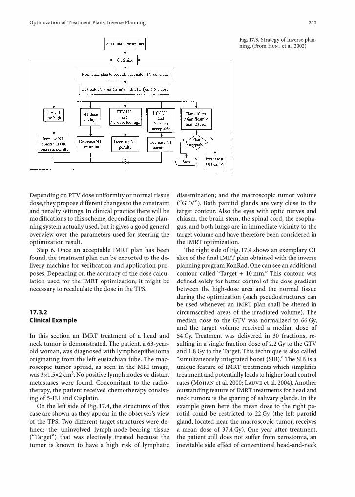
Optimization of Treatment Plans, Inverse Planning 215

Depending on PTV dose uniformity or normal tissue dose, they propose different changes to the constraint and penalty settings. In clinical practice there will be modifi cations to this scheme, depending on the plan-ning system actually used, but it gives a good general overview over the parameters used for steering the optimization result.

Step 6. Once an acceptable IMRT plan has been found, the treatment plan can be exported to the de-livery machine for verifi cation and application pur-poses. Depending on the accuracy of the dose calcu-lation used for the IMRT optimization, it might be necessary to recalculate the dose in the TPS.

17.3.2 Clinical Example

In this section an IMRT treatment of a head and neck tumor is demonstrated. The patient, a 63-year-old woman, was diagnosed with lymphoepithelioma originating from the left eustachian tube. The mac-roscopic tumor spread, as seen in the MRI image, was 3×1.5×2 cm3. No positive lymph nodes or distant metastases were found. Concomitant to the radio-therapy, the patient received chemotherapy consist-ing of 5-FU and Cisplatin.

On the left side of Fig. 17.4, the structures of this case are shown as they appear in the observer’s view of the TPS. Two different target structures were de-fi ned: the uninvolved lymph-node-bearing tissue (“Target”) that was electively treated because the tumor is known to have a high risk of lymphatic

dissemination; and the macroscopic tumor volume (“GTV”). Both parotid glands are very close to the target contour. Also the eyes with optic nerves and chiasm, the brain stem, the spinal cord, the esopha-gus, and both lungs are in immediate vicinity to the target volume and have therefore been considered in the IMRT optimization.

The right side of Fig. 17.4 shows an exemplary CT slice of the fi nal IMRT plan obtained with the inverse planning program KonRad. One can see an additional contour called “Target + 10 mm.” This contour was defi ned solely for better control of the dose gradient between the high-dose area and the normal tissue during the optimization (such pseudostructures can be used whenever an IMRT plan shall be altered in circumscribed areas of the irradiated volume). The median dose to the GTV was normalized to 66 Gy, and the target volume received a median dose of 54 Gy. Treatment was delivered in 30 fractions, re-sulting in a single fraction dose of 2.2 Gy to the GTV and 1.8 Gy to the Target. This technique is also called “simultaneously integrated boost (SIB).” The SIB is a unique feature of IMRT treatments which simplifi es treatment and potentially leads to higher local control rates (Mohan et al. 2000; Lauve et al. 2004). Another outstanding feature of IMRT treatments for head and neck tumors is the sparing of salivary glands. In the example given here, the mean dose to the right pa-rotid could be restricted to 22 Gy (the left parotid gland, located near the macroscopic tumor, receives a mean dose of 37.4 Gy). One year after treatment, the patient still does not suffer from xerostomia, an inevitable side effect of conventional head-and-neck

Fig. 17.3. Strategy of inverse plan-ning. (From HUNT et al. 2002)

216 T. Bortfeld and C. Thieke

radiotherapy that can greatly reduce the quality of life. Especially in cases with a very good long-term prog-nosis, like in this example, such considerations are important. Also the doses to all other organs at risk in this case could be kept well below the tolerance level.

17.4 Multicriteria Optimization in Inverse Planning

In the previous sections we saw that inverse planned IMRT is already in use in clinical practice; however, it also became clear that “inverse planning” as done today leaves a lot to be desired, and a lot of research effort is still put into this fi eld. Presently, inverse plan-ning is still a recursive approach that might include several optimization runs and can therefore be quite time-consuming. Setting the optimization param-eters is non-intuitive. The penalty factors are artifi -cial parameters that do not have a clinical meaning, and even the constraints, which should stand for the tolerance doses of the particular organ at risk, are often used as mere steering parameters when they cannot be fulfi lled in every voxel of the structure any-way. The impact of changes to the parameters cannot be seen a priori. Instead, a new optimization run is needed, making changes to the plan non-interactive. The planning might stop when a certain time limit has been reached, not necessarily when the best treat-ment plan for the patient has been found.

A new optimization paradigm, the multicriteria optimization, is a promising concept to overcome these problems. In the following we present the joint effort of the Massachusetts General Hospital (Boston, Mass, USA), the Fraunhofer Institute for Industrial Mathematics (Kaiserslautern, Germany), and the German Cancer Research Center (Heidelberg, Germany; Küfer et al. 2000; Bortfeld et al. 2002; Küfer et al. 2003; Thieke 2003).

To motivate multicriteria optimization, it is help-ful to step back and look at the original optimization problem: There is a target structure which should be treated with full dose, and there are organs at risk nearby that should receive as little dose as possible. But even with IMRT, due to the physical properties of photon beams (namely, the depth-dose curve with an exponential tail and the penumbra), it is impossible to deliver the ideal dose distribution, which is 100% in the target and 0% everywhere else; therefore, ev-ery treatment plan is a certain compromise between these confl icting goals. Mathematically speaking, the optimization problem does not have a single solution where all criteria are at their individual optimum at the same time. This is exactly the defi nition of a mul-ticriteria optimization problem. Instead of a single optimum, there is a whole solution space of optimal compromises, also called Pareto optimal solutions. A compromise is Pareto optimal when it cannot be improved in one criterion without worsening at least on other criterion. The whole set of Pareto optimal solutions is called the Pareto front.

Leftparotid

LeftLung

Rightparotid

Right Lung

SpinalCord

Target

Brainstem

Opticnerves

Eyes

Chiasm

Fig. 17.4. Organ contours and dose distribution of the IMRT head and neck case

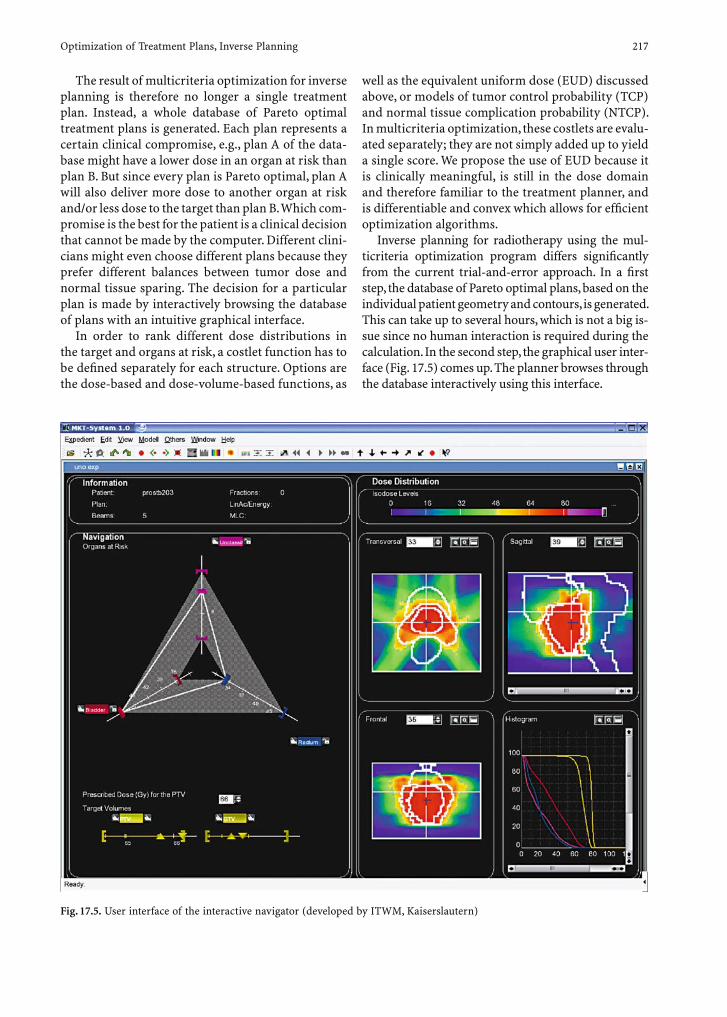
Optimization of Treatment Plans, Inverse Planning 217

The result of multicriteria optimization for inverse planning is therefore no longer a single treatment plan. Instead, a whole database of Pareto optimal treatment plans is generated. Each plan represents a certain clinical compromise, e.g., plan A of the data-base might have a lower dose in an organ at risk than plan B. But since every plan is Pareto optimal, plan A will also deliver more dose to another organ at risk and/or less dose to the target than plan B. Which com-promise is the best for the patient is a clinical decision that cannot be made by the computer. Different clini-cians might even choose different plans because they prefer different balances between tumor dose and normal tissue sparing. The decision for a particular plan is made by interactively browsing the database of plans with an intuitive graphical interface.

In order to rank different dose distributions in the target and organs at risk, a costlet function has to be defi ned separately for each structure. Options are the dose-based and dose-volume-based functions, as

well as the equivalent uniform dose (EUD) discussed above, or models of tumor control probability (TCP) and normal tissue complication probability (NTCP). In multicriteria optimization, these costlets are evalu-ated separately; they are not simply added up to yield a single score. We propose the use of EUD because it is clinically meaningful, is still in the dose domain and therefore familiar to the treatment planner, and is differentiable and convex which allows for effi cient optimization algorithms.

Inverse planning for radiotherapy using the mul-ticriteria optimization program differs signifi cantly from the current trial-and-error approach. In a fi rst step, the database of Pareto optimal plans, based on the individual patient geometry and contours, is generated. This can take up to several hours, which is not a big is-sue since no human interaction is required during the calculation. In the second step, the graphical user inter-face (Fig. 17.5) comes up. The planner browses through the database interactively using this interface.

Fig. 17.5. User interface of the interactive navigator (developed by ITWM, Kaiserslautern)

218 T. Bortfeld and C. Thieke

The user interface is divided into two main win-dows: the left panel shows the part used for the navi-gation. Here the complete database is visualized by a star with one axis for each structure of the treat-ment plan. The gray area shows all EUD values that can be reached for each organ. This way the complete planning horizon becomes apparent at fi rst sight. The planner does not have to fi nd out by trial and error what dose might be achievable in a certain critical structure, instead he just looks at the extreme values on the EUD navigation axes. In addition, the current treatment plan is represented by a polygon connect-ing the EUD values of all structures. The right panel visualizes the current plan as dose volume histogram and as 3D dose distribution in frontal, sagittal, and transverse projection. All plans are normalized to the same target EUD, and the planning horizon can be changed by the global normalization factor.

At the beginning, the system suggests a starting solution. If one or more aspects of the plan are not desirable, e.g., the EUD in one critical structure is too high, the planner can immediately go to another so-lution in which that specifi c criterion is fulfi lled. This is done by grabbing the marker at the EUD bar of the particular organ and dragging it in the desired direction. Instantaneously, the system fi nds the cor-responding solution in its database and updates the information for the other structures and in the DVH and isodose windows.

In our opinion the advantages of this concept are threefold:• Artifi cial weight factors, which have no clinical

meaning, are avoided. The whole concept is based on dose-like values, which are amenable to a clini-cal interpretation.

• Unnecessarily high doses in some of the critical structures, which can occur in constrained opti-mization, are avoided by defi nition of the Pareto optimal solution.

• Plan tuning can be done interactively using “knobs” that have a clinical meaning. It is easy to do a sensitivity analysis and determine the depen-dency of, for example, the target EUD on any of the critical-structure EUDs.

In summary, the planner gains a complete overview over the individual solution space and can choose the compromise that is really the best for the patient, whereby the time required for human intervention is only seconds to minutes. Compared with inverse plan-ning with scalar objective functions, the workload of the treatment planner can be reduced and the quality of the resulting treatment plan can be improved.

Multicriteria optimization for radiotherapy plan-ning as shown in this chapter is still under develop-ment, but when it becomes available in clinical rou-tine it may change the way radiotherapy planning is done in the future.

17.5 Conclusion

Optimized inverse planning can yield superior treat-ment plans, especially in complex situations with convex–concave target volumes and nearby critical structures; however, the optimization criteria must be carefully chosen. Determining appropriate optimiza-tion criteria is not straightforward and requires some trial and error in a “human iteration loop.” Using current commercial inverse planning systems this process can be quite time-consuming. Experienced treatment planners know how to steer an IMRT plan in the desired direction by appropriately changing the optimization criteria. Also, class solutions can help to avoid or reduce the “human iteration loop” in cases that do not vary too much between individu-als, such as prostate treatments, because optimization criteria can be re-used. Nevertheless, plan optimiza-tion leaves something to be desired. The main prob-lem is that it may not be possible to come up with a quantitative, complete optimization formulation for radiotherapy planning in the near future; however, an achievable alternative is to design optimization sys-tems that let the physicians exercise their experienced clinical judgment or intuition in the most direct in-teractive way. Therefore, some future developments aim at a more interactive approach towards inverse planning. Multicriteria optimization and navigating a treatment plan database have been described as promising approaches in this context.

References

Alber M, Nüsslin F (2000) Intensity modulated photon beams subject to a minimal surface smoothing constraint. Phys Med Biol 45:N49–N52

Alber M, Nüsslin F (2001) Optimization of intensity modulated radiotherapy under constraints for static and dynamic MLC delivery. Phys Med Biol 46:3229–3339

Bahr GK, Kereiakes JG, Horwitz H, Finney R, Galvin J, Goode K (1968) The method of linear programming applied to radiation treatment planning. Radiology 91:686–693

Birkhoff G (1940) On drawings composed of uniform straight lines. J Math 19:3

Optimization of Treatment Plans, Inverse Planning 219

Bortfeld T (1999) Optimized planning using physical objec-tives and constraints. Semin Radiat Oncol 9:20–34

Bortfeld T (2003) Physical optimization. In: Palta JR, Mackie TR (eds) Intensity-modulated radiation therapy: the state of the art. Medical Physics Publishing, Madison, Wisconsin, pp 51–76

Bortfeld T, Schlegel W (1993) Optimization of beam orienta-tions in radiation therapy: some theoretical considerations. Phys Med Biol 38:291–304

Bortfeld T, Bürkelbach J, Boesecke R, Schlegel W (1990) Meth-ods of image reconstruction from projections applied to conformation radiotherapy. Phys Med Biol 35:1423–1434

Bortfeld T, Boyer AL, Schlegel W, Kahler DL, Waldron TJ (1994) Realization and verifi cation of three-dimensional confor-mal radiotherapy with modulated fi elds. Int J Radiat Oncol Biol Phys 30:899–908

Bortfeld T, Stein J, Preiser K (1997) Clinically relevant intensity modulation optimization using physical criteria. Twelfth International Conference on the Use of Computers in Radiation Therapy, Salt Lake City, Utah

Bortfeld T, Thieke C, Küfer K.-H., Trinkaus H (2002) New approaches in intensity-modulated radiotherapy: a new optimization paradigm. In: Kogelnik HD, Lukas P, Sedl-mayer F (eds) Progress in radio-oncology, vol 7. Monduzzi Editore, Bologna, pp 251–258

Brahme A (1984) Dosimetric precision requirements in radia-tion therapy. Acta Radiol Oncol 23:379–391

Brahme A (1993) Optimization of radiation therapy and the development of multileaf collimation. Int J Radiat Oncol Biol Phys 25:373–375

Brahme A (1994) Optimization of radiation therapy. Int J Radiat Oncol Biol Phys 28:785–787

Brahme A, Roos JE, Lax I (1982) Solution of an integral equa-tion in rotation therapy. Phys Med Biol 27:1221–1229

Carol MP, Nash RV, Campbell RC, Huber R, Sternick E (1997) The development of a clinically intuitive approach to inverse treatment planning: partial volume prescription and area cost function. Twelfth International Conference on the Use of Computers in Radiation Therapy. Salt Lake City, Utah

Censor Y (2003) Mathematical optimization for the inverse problem of intensity-modulated radiation therapy. Inten-sity-modulated radiation therapy: the state of the art. In: Palta JR, Mackie TR (eds) Medical Physics Publishing, pp 25–49

Censor Y, Altschuler MD, Powlis WD (1988) A computational solution of the inverse problem in radiation-therapy treat-ment planning. Appl Math Comput 25:57–87

Cho PS, Marks RJ II (2000) Hardware-sensitive optimiza-tion for intensity modulated radiotherapy. Phys Med Biol 45:429–440

Cho PS, Lee S, Marks RJ II, Oh S, Sutlief SG, Phillips MH (1998) Optimization of intensity modulated beams with volume constraints using two methods: cost function minimization and projections onto convex sets. Med Phys 25:435–443

Chui CS, Chan MF, Yorke E, Spirou S, Ling CC (2001) Delivery of intensity-modulated radiation therapy with a conven-tional multileaf collimator: comparison of dynamic and segmental methods. Med Phys 28:2441–2449

Cormack AM, Cormack RA (1987) A problem in rotation ther-apy with X-rays: dose distributions with an axisof symme-try. Int J Radiat Oncol Biol Phys 13:1921–1925

Deasy JO (1997) Multiple local minima in radiotherapy opti-

mization problems with dose-volume constraints. Med Phys 24:1157–1161

DeNeve W, DeWagter C, DeJaeger K, Thienpont M, Colle C, Derycke S, Schelfhout J (1996) Planning and delivering high doses to targets surrounding the spinal cord atthe lower neck and upper mediastinal levels: static beam-seg-mentation technique executed with a multileaf collimator. Radiother Oncol 40:271–279

Fraass B (2002) Differences between plan evaluation and the optimization problem statement, and the difference it makes. http://www.isye.gatech.edu/nci-nsf.orart.2002/talks.php.

Gustafsson A, Langer M (2000) Dose-volume constrained radiotherapy optimization for a clinical treatment plan-ning system. Thirteenth International Conference on the use of Computers in Radiation therapy. Springer, Berlin Heidelberg New York

Gustafsson A, Lind BK, Brahme A (1994) A generalized pencil beam algorithm for optimization of radiation therapy. Med Phys 21:343–356

Holmes T, Mackie TR, Simpkin D, Reckwerdt P (1991) A uni-fi ed approach to the optimization of brachytherapy and external beam dosimetry. Int J Radiat Oncol Biol Phys 20:859–873

Hope CS, Laurie J, Orr JS, Halnan KE (1967) Optimization of X-ray treatment planning by computer judgement. Phys Med Biol 12:531–542

Hunt MA, Hsiung CY, Spirou SV, Chui CS, Amols HI, Ling CC (2002) Evaluation of concave dose distributions created using an inverse planning system. Int J Radiat Oncol Biol Phys 54:953–962

ICRU (1993) Prescribing, recording, and reporting photon beam therapy. International Commission on Radiation Units and Measurements, report 50. Bethesda, Maryland

IMRT (2001) Intensity-modulated radiotherapy: current status and issues of interest. Int J Radiat Oncol Biol Phys 51:880–914

Keller-Reichenbecher M-A, Bortfeld T, Levegrün S, Stein J, Preiser K, Schlegel W (1998) Intensity modulation with the step and shoot technique using a commercial MLC: a plan-ning study. Int J Radiat Oncol Biol Phys 45:1315–1324

Kessen A, Grosser K-H, Bortfeld T (2000) Simplifi cation of IMRT intensity maps by means of 1-D and 2-D median-fi ltering during the iterative calculation. Thirteenth Inter-national Conference on the Use of Computers in Radiation therapy. Springer, Berlin Heidelberg New York

Küfer K-H, Hamacher HW, Bortfeld TR (2000) A multicriteria optimization approach for inverse radiotherapy planning. Proc XIIIth ICCR, Heidelberg 2000. Springer, Berlin Heidel-berg New York, pp 26–29

Küfer K-H, Scherrer A, Monz M, Alonso F, Trinkaus H, Bort-feld T, Thieke C (2003) Intensity modulated radiotherapy: a large scale multi-criteria programming problem. OR Spec-trum 25:223–249

Kwa SL, Lebesque JV, Theuws JC, Marks LB, Munley MT, Bentel G, Oetzel D, Spahn U, Graham MV, Drzymala RE, Purdy JA, Lichter AS, Martel MK, Ten Haken RK (1998) Radiation pneumonitis as a function of mean lung dose: an analysis of pooled data of 540 patients. Int J Radiat Oncol Biol Phys 42:1–9

Langer M, Leong J (1989) Optimization of beam weights under dose-volume restrictions. Int J Radiat Oncol Biol Phys 13:1255–1259

220 T. Bortfeld and C. Thieke

Langer M, Brown R, Urie M, Leong J, Stracher M, Shapiro J (1990) Large scale optimization of beam weights under dose-volume restrictions. Int J Radiat Oncol Biol Phys 18:887–893

Langer M, Morrill S, Brown R, Lee O, Lane R (1996) A com-parison of mixed integer programming and fast simulated annealing for optimizing beam weights in radiation ther-apy. Med Phys 23:957–964

Langer M, Lee EK, Deasy JO, Rardin RL, Deye JA (2003) Opera-tions research applied to radiotherapy, an NCI-NSF-spon-sored workshop 7–9 February, 2002. Int J Radiat Oncol Biol Phys 57:762–768

Lauve A, Morris M, Schmidt-Ullrich R, Wu Q, Mohan R, Abayomi O, Buck D, Holdford D, Dawson K, Dinardo L, Reiter E (2004) Simultaneous integrated boost intensity-modulated radiotherapy for locally advanced head-and-neck squamous cell carcinomas. Part II: clinical results. Int J Radiat Oncol Biol Phys 60:374–387

Levegrun S, Jackson A, Zelefsky MJ, Skwarchuk MW, Venkatra-man ES, Schlegel W, Fuks Z, Leibel SA, Ling CC (2001) Fit-ting tumor control probability models to biopsy outcome after three-dimensional conformal radiation therapy of prostate cancer: pitfalls in deducing radiobiologic param-eters for tumors from clinical data. Int J Radiat Oncol Biol Phys 51:1064–1080

Llacer J, Deasy JO, Portfeld TR, Solberg TD, Promberger C (2003) Absence of multiple local minima effects in inten-sity modulated optimization with dose-volume constraints. Phys Med Biol 48:183–210

Mackie R, Deasy J, Holmes T, Fowler J (1994) Optimization of radiation therapy and the development of multileaf col-limation. Int J Radiat Oncol Biol Phys 28:784–785

McDonald SC, Rubin P (1977) Optimization of external beam radiation therapy. Int J Radiat Oncol Biol Phys 2:307–317

Mohan R, Ling CC (1995) When becometh less more? Int J Radiat Oncol Biol Phys 33:235–237

Mohan R, Wang XH (1996) Physical vs biological objectives for treatment plan optimization. Radiother Oncol 40:186–187

Mohan R, Wu Q, Manning M, Schmidt-Ullrich R (2000) Radiobiological considerations in the design of fraction-ation strategies for intensity-modulated radiation therapy of head and neck cancers. Int J Radiat Oncol Biol Phys 46:619–630

Natterer F (1986) The mathematics of computerized tomogra-phy. Teubner, Stuttgart

Niemierko A (1992) Random search algorithm (RONSC) for the optimization of radiation therapy with both physi-cal and biological endpoints and constraints. Int J Radiat Oncol Biol Phys 23:89–98

Niemierko A (1997) Reporting and analyzing dose distribu-tions: a concept of equivalent uniform dose. Med Phys 24:103–110

Niemierko A (1999) A generalized concept of equivalent uni-form dose (EUD). Med Phys 26:1100

Pugachev A, Li JG, Boyer AL, Hancock SL, Le QT, Donaldson SS, Xing L (2001) Role of beam orientation optimization in intensity-modulated radiation therapy. Int J Radiat Oncol Biol Phys 50:551–560

Redpath AT, Vickery BL, Wright DH (1975) A set of fortran subroutines for optimizing radiotherapy plans. Comput Programs Biomed 5:158–164

Romeijn HE, Ahuja RK, Dempsey JF, Kumar A, Li JG (2003) A novel linear programming approach to fl uence map opti-mization for intensity modulated radiation therapy treat-ment planning. Phys Med Biol 48:3521–3542

Shepard DM, Earl MA, Li XA, Naqvi S, C Yu (2002) Direct aper-ture optimization: a turn key solution for step-and-shoot IMRT. Med Phys 29:1007–1018

Shepard DM, Ferris MC, Olivera GH, Mackie TR (1999) Opti-mizing the delivery of radiation therapy to cancer patients. SIAM Rev 41:721–733

Söderström S, Brahme A (1995) Which is the most suitable number of photon beam portals in coplanar radiation therapy. Int J Radiat Oncol Biol Phys 33:151–159

Söderström S, Brahme A (1996) Small is beautiful: and often enough. Int J Radiat Oncol Biol Phys 34:757–758

Spirou SV, Chui C-S (1998) A gradient inverse planning algo-rithm with dose-volume constraints. Med Phys 25:321–333

Starkschall G, Pollack A, Stevens CW (2000) Using a dose-volume feasibility search algorithm for radiation treatment planning. Thirteenth International Conference on the Use of Computers in Radiation therapy. Springer, Berlin Hei-delberg New York

Stein J, Mohan R, Wang XH, Bortfeld T, Wu Q, Preiser K, Ling CC, Schlegel W (1997) Number and orientation of beams in intensity-modulated radiation treatments. Med Phys 24:149–160

Thieke C (2003) Multicriteria optimization in inverse radio-therapy planning. Doctor of Natural Sciences dissertation. Combined Faculties for the Natural Sciences and for Math-ematics, Ruperto-Carola University of Heidelberg

Thieke C, Bortfeld T, Niemierko A (2002) Direct Consider-ation of EUD Constraints in IMRT Optimization. Med Phys 29:1283

Webb S (1989) Optimisation of conformal radiotherapy dose distributions by simulated annealing. Phys Med Biol 34:1349–1370

Webb S (1992) Optimization by simulated annealing of three-dimensional, conformaltreatment planning for radiation fi elds defi ned by a multileaf collimator:II. Inclusion of the two-dimensional modulation of the X-ray intensity. Phys Med Biol 37:1689–1704

Webb S, Convery DJ, Evans PM (1998) Inverse planning with constraints to generate smoothed intensity-modulated beams. Phys Med Biol 43:2785–2794

Wu Q, Mohan R (2002) Multiple local minima in IMRT optimiza-tion based on dose-volume criteria. Med Phys 29:1514–1527

Wu Q, Mohan R, Niemierko A, Schmidt-Ullrich R (2002) Opti-mization of intensity-modulated radiotherapy plans based on the equivalent uniform dose. Int J Radiat Oncol Biol Phys 52:224–235

Yajnik S, Rosenzweig KE, Mychalczak B, Krug L, Flores R, Hong L, Rusch VW (2003) Hemithoracic radiation after extra-pleural pneumonectomy for malignant pleural mesothe-lioma. Int J Radiat Oncol Biol Phys 56:1319–1326

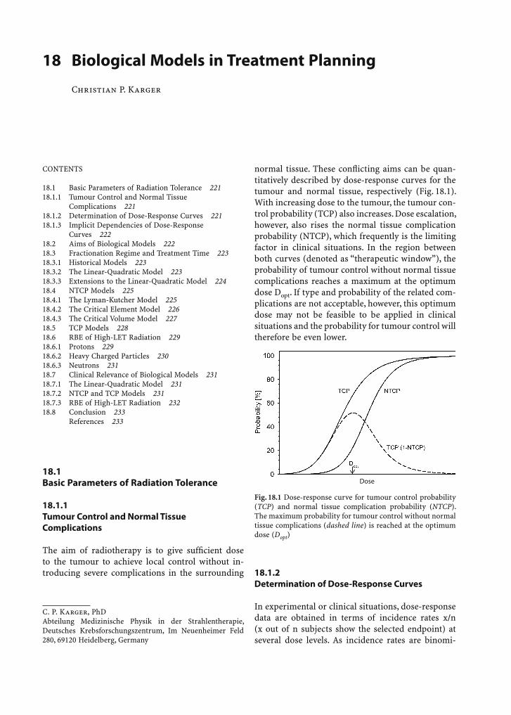
Biological Models in Treatment Planning 221

18 Biological Models in Treatment Planning

Christian P. Karger

C. P. Karger, PhDAbteilung Medizinische Physik in der Strahlentherapie, Deutsches Krebsforschungszentrum, Im Neuenheimer Feld 280, 69120 Heidelberg, Germany

18.1 Basic Parameters of Radiation Tolerance

18.1.1 Tumour Control and Normal Tissue Complications

The aim of radiotherapy is to give suffi cient dose to the tumour to achieve local control without in-troducing severe complications in the surrounding

normal tissue. These confl icting aims can be quan-titatively described by dose-response curves for the tumour and normal tissue, respectively (Fig. 18.1). With increasing dose to the tumour, the tumour con-trol probability (TCP) also increases. Dose escalation, however, also rises the normal tissue complication probability (NTCP), which frequently is the limiting factor in clinical situations. In the region between both curves (denoted as “therapeutic window”), the probability of tumour control without normal tissue complications reaches a maximum at the optimum dose Dopt. If type and probability of the related com-plications are not acceptable, however, this optimum dose may not be feasible to be applied in clinical situations and the probability for tumour control will therefore be even lower.

CONTENTS

18.1 Basic Parameters of Radiation Tolerance 22118.1.1 Tumour Control and Normal Tissue Complications 22118.1.2 Determination of Dose-Response Curves 22118.1.3 Implicit Dependencies of Dose-Response Curves 22218.2 Aims of Biological Models 22218.3 Fractionation Regime and Treatment Time 22318.3.1 Historical Models 22318.3.2 The Linear-Quadratic Model 22318.3.3 Extensions to the Linear-Quadratic Model 22418.4 NTCP Models 22518.4.1 The Lyman-Kutcher Model 22518.4.2 The Critical Element Model 22618.4.3 The Critical Volume Model 22718.5 TCP Models 22818.6 RBE of High-LET Radiation 22918.6.1 Protons 22918.6.2 Heavy Charged Particles 23018.6.3 Neutrons 23118.7 Clinical Relevance of Biological Models 23118.7.1 The Linear-Quadratic Model 23118.7.2 NTCP and TCP Models 23118.7.3 RBE of High-LET Radiation 23218.8 Conclusion 233 References 233

Fig. 18.1 Dose-response curve for tumour control probability (TCP) and normal tissue complication probability (NTCP). The maximum probability for tumour control without normal tissue complications (dashed line) is reached at the optimum dose (Dopt)

18.1.2 Determination of Dose-Response Curves

In experimental or clinical situations, dose-response data are obtained in terms of incidence rates x/n (x out of n subjects show the selected endpoint) at several dose levels. As incidence rates are binomi-

Dose

222 C. P. Karger

ally distributed and show a large spread for a small number of subjects, n, an analytical curve is adjusted to the data using a maximum likelihood fi t. Although several parameterisations may be used to describe dose-response curves mathematically (Källman et al. 1992; Niemierko and Goitein 1991), the follow-ing one is frequently used because of its simplicity:

P DDD

k( ) =+ ⎛⎝⎜

⎞⎠⎟

1

1 50

(1)

P(D) gives the expectation value of the probability that the selected end point occurs at the dose level D. The parameter D50 (often referred to as tolerance dose, TD50, or equivalent dose, ED50) is the dose at which an effect probability of 50% is expected. The parameter k is related to the slope of the dose-re-sponse curve.

Most statistical software packages supply the lo-gistic formula for parameterisation of dose-response curves, which is not equivalent to Eq. (1). The parame-ters D50 and k of Eq. (1) as well as their standard errors, however, may be calculated from the fi t of the logistic function, if ln(D) instead of the dose D is used as inde-pendent variable (Karger and Hartmann 2001).

Tolerance doses for normal tissue complications may be determined with reasonable accuracy in ani-mal experiments. The question of whether these data also apply to humans, however, remains an intrinsic problem, and tolerance doses from animal experi-ments are generally not believed to be directly trans-ferable to humans. In humans, on the other hand, the parameter D50 usually cannot be determined as such high complication rates are usually prevented by clin-ical experience. For clinical applications, quantities such as D5 (dose leading to 5% complication prob-ability) are more relevant. From such low complica-tion probabilities, however, it is nearly impossible to determine the slope of the curve.

Emami et al. (1991) published a compilation of data for D5 and D50 for a variety of normal tissues. Although the authors stressed the limited accuracy of these data, no signifi cant improvements in knowl-edge was achieved up to now and most articles still refer to these data.

18.1.3 Implicit Dependencies of Dose-Response Curves

Figure 18.1 suggests that the effect probability is solely a function of the radiation dose. The dose-

response curves, however, implicitly depend on sev-eral biological and physical parameters. At fi rst, the biological end point for the tissue response has to be specifi ed, including the time after radiation used for follow-up. For normal tissue complications, the dose-response curves will be different for early and late effects and even within one type of complication the curves may differ, depending on the exact end point defi nition and the method of investigation. In the same way, the curve for the tumour may depend on the defi nition of tumour control, e.g. whether lo-cal control or remission of the tumour is regarded. In the clinical situation, relevant end points have to be selected, e.g. radiological tumour control and early or late complications which are defi nitely to be pre-vented.

Besides the defi nition of the biological end point, the dose-response curves are strongly infl uenced by various treatment parameters, most of them being of physical nature. The most important parameters are given by the time pattern of the applied dose, the volume of irradiated normal tissue and the radiation quality used for treatment. Since the very beginning of radiotherapy treatments, it was the aim of many investigations to optimise the physical treatment pa-rameters to improve clinical outcome, i.e. to open the “therapeutic window” between the dose-response curves for tumour control and normal tissue compli-cations (Fig. 18.1).

18.2 Aims of Biological Models

The aim of biological models is to predict the ra-diation response of biological systems. While early approaches focused on modelling the radiation re-sponse for different fractionation schemes, newer developments attempt to model effect probabilities (TCP and NTCP), their volume dependence and the relative biological effi ciency (RBE) of radiation with high linear energy transfer (LET).

In treatment planning, biological models may be applied with different intentions:1. Transfer of one treatment regime to a biologically

iso-effective new regime or new radiation modal-ity without predicting absolute values for TCP or NTCP.

2. Calculation of TCP or NTCP values to compare either competing treatment plans for an individ-ual patient or different treatment techniques for a specifi ed clinical application. In this case, the TCP/

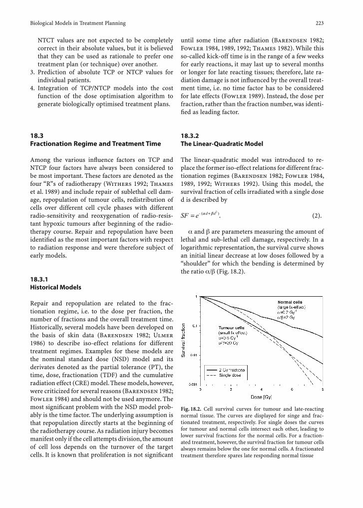
Biological Models in Treatment Planning 223

NTCT values are not expected to be completely correct in their absolute values, but it is believed that they can be used as rationale to prefer one treatment plan (or technique) over another.

3. Prediction of absolute TCP or NTCP values for individual patients.

4. Integration of TCP/NTCP models into the cost function of the dose optimisation algorithm to generate biologically optimised treatment plans.

18.3 Fractionation Regime and Treatment Time

Among the various infl uence factors on TCP and NTCP four factors have always been considered to be most important. These factors are denoted as the four “R”s of radiotherapy (Withers 1992; Thames et al. 1989) and include repair of sublethal cell dam-age, repopulation of tumour cells, redistribution of cells over different cell cycle phases with different radio-sensitivity and reoxygenation of radio-resis-tant hypoxic tumours after beginning of the radio-therapy course. Repair and repopulation have been identifi ed as the most important factors with respect to radiation response and were therefore subject of early models.

18.3.1 Historical Models

Repair and repopulation are related to the frac-tionation regime, i.e. to the dose per fraction, the number of fractions and the overall treatment time. Historically, several models have been developed on the basis of skin data (Barendsen 1982; Ulmer 1986) to describe iso-effect relations for different treatment regimes. Examples for these models are the nominal standard dose (NSD) model and its derivates denoted as the partial tolerance (PT), the time, dose, fractionation (TDF) and the cumulative radiation effect (CRE) model. These models, however, were criticized for several reasons (Barendsen 1982; Fowler 1984) and should not be used anymore. The most signifi cant problem with the NSD model prob-ably is the time factor. The underlying assumption is that repopulation directly starts at the beginning of the radiotherapy course. As radiation injury becomes manifest only if the cell attempts division, the amount of cell loss depends on the turnover of the target cells. It is known that proliferation is not signifi cant

until some time after radiation (Barendsen 1982; Fowler 1984, 1989, 1992; Thames 1982). While this so-called kick-off time is in the range of a few weeks for early reactions, it may last up to several months or longer for late reacting tissues; therefore, late ra-diation damage is not infl uenced by the overall treat-ment time, i.e. no time factor has to be considered for late effects (Fowler 1989). Instead, the dose per fraction, rather than the fraction number, was identi-fi ed as leading factor.

18.3.2 The Linear-Quadratic Model

The linear-quadratic model was introduced to re-place the former iso-effect relations for different frac-tionation regimes (Barendsen 1982; Fowler 1984, 1989, 1992; Withers 1992). Using this model, the survival fraction of cells irradiated with a single dose d is described by

− +( )α βSF e d d=2

. (2).

and are parameters measuring the amount of lethal and sub-lethal cell damage, respectively. In a logarithmic representation, the survival curve shows an initial linear decrease at low doses followed by a “shoulder” for which the bending is determined by the ratio / (Fig. 18.2).

Fig. 18.2. Cell survival curves for tumour and late-reacting normal tissue. The curves are displayed for singe and frac-tionated treatment, respectively. For single doses the curves for tumour and normal cells intersect each other, leading to lower survival fractions for the normal cells. For a fraction-ated treatment, however, the survival fraction for tumour cells always remains below the one for normal cells. A fractionated treatment therefore spares late responding normal tissue

224 C. P. Karger

The smaller / is, the more pronounced the shoulder of the survival curve will be. If the time be-tween two fractions exceeds the minimum of about 6 h (Fowler 1989), the sub-lethal damage can be re-paired and the shape of the cell survival curve will be reproduced for the subsequent fraction (Fig. 18.2). After n fractions of equal doses, d, the survival frac-tion will then be α βe n d d− +( )2

. As the survival level is determined by n d d( )α β+ 2 , a biologically effective dose (also termed as extrapolated response dose, ERD) may be defi ned (Fowler 1989, 1992; Prasad 1992) by the equation

BED nd d= +(/

)1α β

. (3)

Two fractionation regimes having the same BED are considered to be iso-effective. As a consequence, one fractionation regime may be converted to an-other iso-effective regime using the relation

n d n d dd2 2 1 1

1

2

= ⋅ ++

α βα β

//

(4)

n1, n2, and d1, d2 are the number of fractions and the doses per fraction for both regimes, respectively. It is a great advantage of the linear-quadratic model that only the ratio / , rather than the absolute val-ues of and are required in Eq. (4).

Values for / can be measured for in vitro as well as for in vivo systems. Although the same cell type may be involved, the / -values may be different as cells in intact tissue are not expected to respond inde-pendently from their physiological environment. As in vivo settings do not allow to determine the fraction of surviving cells, / has to be measured by equat-ing the BED of two different fractionation regimes according to Eq. (3). The required iso-effective total doses may be obtained from the dose-response curve of the respective regime (e.g. the tolerance doses D50). The resulting equation can then be resolved for / . Alternatively, the inverse of the total dose (nd )-1 may be plotted against the dose per fraction d (referred to as Douglas-Fowler plot) for more than two iso-effective fractionation regimes (Barendsen 1982; Fowler 1984; Thames 1982). According to Eq. (3),

/ may then be determined from a linear regression to the data.

The value for / does not only depend on the irradiated type of tissue, but also on the consid-ered biological end point. Values for / are given in the literature for various tissues and end points (Barendsen 1982; Fowler 1984, 1989; Thames et al. 1989; Withers 1992). Typical / -values are around 3 Gy for late reactions and around 10 Gy for early re-

actions. Most tumours show / -values of 10 Gy or more. As a consequence, late reacting tissue can be spared by fractionated treatment relative to the tu-mour response, while the fractionation effect is small or may even be neglected for early reacting tissues. For these tissues the overall treatment time is more important.

Although attempts have been made to derive Eq. (2) as an approximation from mechanistic con-siderations (Gilbert 1980), the linear-quadratic model is mostly regarded as an empirical parame-terisation. The linear-quadratic model has been vali-dated in the dose range of about 2–8 Gy per fraction (Fowler 1984, 1989; Withers 1986, 1992). At higher doses some experimental cell survival curves asymp-totically approach to a purely exponential shape and deviations to the linear-quadratic model have been seen. This behaviour may be explained by multi-hit killing from accumulation of multiple sub-lethal events (Withers 1992). Although there are other parameterisations for cell survival curves (e.g. the two-component model), which account for the purely exponential shape at high doses, the linear-quadratic model is usually preferred since the derived iso-ef-fect relation of Eq. (4) depends only on the single parameter / (Withers 1992). Because of the limi-tation of the linear-quadratic model at high doses, Eq. (4) should not be used to transfer a fractionated treatment to an iso-effective single dose treatment, although it has previously been used as approxima-tion (Larson et al. 1993; Prasad 1992; Flickinger et al. 1990).

18.3.3 Extensions to the Linear-Quadratic Model

Several extensions have been developed for the lin-ear-quadratic model to account for additional depen-dencies of the radiation response. As repopulation may play an important role for early reacting tissues, a time factor has been introduced:

SF e d d T Tk= − + + −( ) ( )α β γ2

(5),

where is related to the average doubling time Tp of the cells by = In2/Tp and Tk is the kick-off time un-til proliferation starts (Fowler 1989, 1992). For late effects the time factor can be neglected and in this case Eq. (5) reduces to Eq. (2). Equation (5) leads to a modifi ed expression for the BED given by

BED nd d T Tk= + − −(/

) ( )1α β

γα

. (6)

Biological Models in Treatment Planning 225

The apparent disadvantage of this extended model is that the absolute values of is required which is not always available with suffi cient accuracy. In addi-tion, the values of the two parameters and Tk have to be known.

As there is some evidence that and depend on the cell cycle phase, the linear-quadratic model was extended to account for this heterogeneity (Schultheiss 1987). To do so, three additional pa-rameters are introduced, describing the spread and the correlation of the parameters and . In an other approach it was attempted to give a complete descrip-tion for repair, repopulation, redistribution and re-oxygenation (Brenner 1995). This model also needs fi ve input parameters.

A special situation is given by the application of brachytherapy techniques, since the irradiation is performed either continuously over several days or in a fractionated fashion, where the time between the fractions is in the order of one hour. In both cases, the sub-lethal damage may not completely be re-paired. Several investigations have been performed to model the radiation response for incomplete re-pair (Brenner and Hall 1991; Dale 1986; Dale et al. 1988; Ling and Chui 1993; Nilsson et al. 1990; Pop et al. 1996; Thames 1985). As a result, the cell survival curve for incomplete repair is given as

− +( )α βSF e d G d=2

, (7)

where G is a factor calculated from the temporal char-acteristics of the dose distribution (Brenner and Hall 1991). In the case of complete repair, G is equal to 1 and Eq. (7) reduces to Eq. (2). For continuous radiation G is given by

G tT

Tt

eTt= ⎛

⎝⎜⎞⎠⎟

− +⎡

⎣⎢⎢

⎤

⎦⎥⎥

−2 10

2

0

0 , (8)

where T and t0 are the total time of irradiation and the characteristic repair time, respectively (Brenner and Hall 1991; POP et al. 1996). t0 is related to the repair half time T1/2 by T1/2 = t0 In2. For a general fractionation regime of n equal fractions, each of du-ration TF and period t between fractions, the factor G may be calculated according to Brenner 1991:

GnT

nt T ntxF

F= + −⎛⎝⎜

⎞⎠⎟+2 1 1

2 0 02

( )⎡

⎣⎢

t xx

ny

y yN

+ −⎛⎝⎜

⎞⎠⎟ −

− −1 21

102 ( )

(11 2−⎧⎨⎩

⎫⎬⎭

⎤

⎦⎥y). (9)

In Eq. (9) the abbreviations T tx e F= − / 0 and y e t t= −∆ / 0 have been used. For a standard fractionation regime with TF<<t0 and t>>t0, G reduces to 1/N and Eq. (7) then will be reduced to n d( )− +α βSF e d=

2

, which is the product of the survival fractions of n biologically in-dependent fractions.

18.4 NTCP Models

The NTCP models aim to describe the complication probability in normal tissues in terms of dose-re-sponse curves. As there is extensive evidence, that the radiation response of normal tissue depends on the amount of irradiated normal tissue (Burman et al. 1991; Cohen 1982; Emami et al. 1991; Flickinger et al. 1990; Schultheiss 1983; Withers et al. 1988), the irradiated volume is included as an additional im-portant parameter. The extent of the volume effect is dependent on the architecture of the respective tissue and several models have been proposed. While some of them are only of phenomenological nature, others include more basic bio-statistical principles.

18.4.1 The Lyman-Kutcher Model

A four-parameter model was proposed by Lyman (Lyman 1985). In this model, the complication prob-ability P(D, ) for a uniform irradiation of a normal tissue volume V with a dose D is given by (Burman et al. 1991; Burman 2002; Lyman 1985; Kutcher 1996):

P D e dxxt

( , )νπ

=−

−∞∫

12

2

2 (10a)

tm

DTD

= −⎛

⎝⎜

⎞

⎠⎟

1 150 ( )ν

(10b)

TD TD n50 50 1( ) ( )ν ν= ⋅ − (10c)

ν = VVref

. (10d)

The four parameters of the model are given by TD50, m, n and Vref, which have to be adjusted to

226 C. P. Karger

clinical data for each tissue type using a specifi ed biological end point. TD50( ) is the tolerance dose for the fractional volume , m is related to the slope of the dose-response curve, n describes the volume effect and Vref is the reference volume to which the fractional volume refers to. Vref may be chosen as the whole organ or as a part of it. Equation (10c) relates the tolerance doses of the partial volume to that of the reference volume ( =1).

Emami et al. (1991) published tolerance doses for various tissues and fractional volumes which were derived from a literature search and from clinical ex-perience. The authors considered the uncertainty of these tolerance doses to be rather high. Subsequently, the model parameters of Eq. (10) were adjusted to fi t these tolerance data (Burman et al. 1991). As there were only few tolerance doses for each organ, the pa-rameters were fi t “by eye” rather than by using statis-tical methods; therefore, and due to the uncertainty of the underlying data, the derived model parameters have to be treated with great caution. Although some of the tolerance doses were refi ned later (Burman 2002), most of them have remained unchanged up to now.

In clinical practice, the normal tissue will not be uniformly irradiated as assumed by the Lyman model; therefore, the model was extended by introducing histogram-reduction algorithms, which transform the multi-step dose volume histogram obtained for a specifi c treatment plan into a biologically iso-effec-tive single-step histogram, i.e. a non-uniform irra-diation is transformed in an biologically iso-effective uniform irradiation. Two different types of reduction algorithms have been proposed which lead to similar although not identical NTCP-values:

The fi rst one (Lyman and Wolbarst 1987, 1989) replaces the two rightmost bins (at doses Dn and Dn-1 and volumes Vn and Vn-1) of the cumulative histogram by a single bin at dose D n-1 and Volume Vn-1. The dose D n-1 is calculated such that the new histogram has the same NTCP according to Eq. (10). This procedure is iterated until a single-step histogram is achieved which corresponds to a homogeneous irradiation of the reference volume ( =1) with a dose D1 for which the Lyman model can directly be applied.

The second algorithm (Kutcher and Burman 1989; Kutcher et al. 1991) transforms the initial multi-step histogram (having the maximum dose Dmax) to a biologically iso-effective single-step his-togram with an effective volume Veff at the dose Dmax. For this approach, a volume effect according to Eq. (10c) is assumed. The single-step histogram then corresponds to a homogeneous irradiation of the

fractional volume eff = Veff / Vref and the NTCP is then calculated by Eq. (10).

18.4.2 The Critical Element Model

The critical element model (Niemierko and Goitein 1991; Schultheiss 1983; Wolbarst 1984) assumes that an organ consists of a number of identical func-tional subunits (FSU; Withers et al. 1988), each of them responding independently to radiation. The term “critical element” means that it is additionally assumed that a complication occurs, if a single FSU is inactivated (Niemierko and Goitein 1991). The critical element model is expected to describe the radiation response for organs such as spinal cord, brain or bowel.If P(D, ) is the complication probability that a dose D to the fractional volume will produce a compli-cation, [1- P(D, )] is the probability that no com-plication occurs. If a whole organ consisting of N equal-sized compartments (each of volume =1/N) is uniformly irradiated with a dose D, the probabil-ity that the organ escapes injury P(D,1) is given by the product of the probabilities that each sub-vol-ume escapes injury. P(D, ) can then be expressed by (Schultheiss 1983):

P D P D( , ) [ ( , )]ν ν= − −1 1 1 (11)

Equation (11) may easily be generalized to non-uniform dose distributions {D} by replacing the right side by 1- 1 1[ ( , )]−∏ P Di

i

i∆v .

As the size of the product is strongly affected by the smallest factor, the size of the complication prob-ability P(D, ) is governed by large values of P(Di,1), i.e. by the highest doses of {Di}.

It follows from Eq. (11) that the dose-response curve for any partial volume irradiation can be calcu-lated if the dose-response curve for the whole organ is known. No specifi c dose-response model has to be assumed.

It is a characteristic feature of the critical element model that the dose-volume iso-effect curve is de-termined solely by the slope parameter (k in Eq. (1) and m in Eq. (10b), respectively) of the dose-response curve for the whole organ (Niemierko and Goitein 1991). In contrast to this, the volume dependence in the Lyman model (Eq. (10c)) uses the additional pa-rameter n, which can be selected independently from the slope parameter m. That means that in general,

Biological Models in Treatment Planning 227

the Lyman model describes a tissue architecture dif-ferent from the one of the critical element model.In the approximation of P(D,1)<<1 (i.e. small doses, D<<D50), however, Eq. (11) yields P D, )) (P D( ,ν ν= ⋅ 1 . If in addition the dose-response model of Eq. (1) is taken in the same approximation one obtains P D D D k( , ) ( / )1 = . From these two relations, a dose-volume iso-effect relation can be derived (Schultheiss 1983):

= ⋅D Dkν ν −1

1 (12)

This relation is of the same structure as Eq. (10c). This means that the Lyman model is able to describe the dose-volume relation of tissue with critical ele-ment structure only for small complication probabili-ties (Niemierko and Goitein 1991). It also has to be pointed out that the histogram reduction methods (Lyman and Wolbarst 1987, 1989; Kutcher and Burman 1989; Kutcher et al. 1991) of the Lyman model implicitly make use of Eq. (10c) which is in gen-eral not valid for tissues with critical element struc-ture. In this case the algorithms have to be adapted according to Niemierko and Goitein (1991).

The two dose-volume relations of Eqs. (11) and (12) were tested in animal experiments for the spi-nal cord and the brain, which both are considered to be of the critical element architecture (Niemierko and Goitein 1991; Schultheiss 1983). As expected, Eq. (11) was found to give a better description of the data. The critical element model was also used to cal-culate the complication probabilities and dose-vol-ume iso-effect relations for radiosurgery treatments of the brain (Lax and Karlsson 1996; Flickinger 1989; Flickinger et al. 1990).

Although the publication of Schultheiss (1983) does not explicitly use the term “FSU”, the described model comprises all characteristic features of the critical element model. A more theoretical approach was presented by Wolbarst (1984), using the dose-response curve of a single FSU as starting point to model the radiation response of the entire organ.

18.4.3 The Critical Volume Model

The critical volume model describes tissues, where the FSUs of an organ are assumed to be arranged in a parallel fashion (Jackson et al. 1993; Niemierko and Goitein 1993a; Wolbarst et al. 1982; Yorke et al. 1993). In contrast to the critical element model, an inactivation of a single FSU will not lead to a

complication in the organ as the organ function will be maintained by the remaining FSUs. If more than a critical number of FSUs will be inactivated, however, a complication will occur. This especially means that the organ tolerates any dose as long as the number of affected FSUs is below this threshold. The critical volume model is expected to describe the complica-tion probabilities of organs such as the lung, kidney, liver, or parotid glands.

If an organ is assumed to consist of N parallel organized and independently responding FSUs, the probability that more than M FSUs are inactivated by an uniform dose D is given by (Niemierko and Goitein 1993a):

P DNk

P PFSUk

FSUN k

k M

N

( ) ( )=⎛

⎝⎜

⎞

⎠⎟ ⋅ − −

= +∑ 1

1, (13)

where PFSU is the dose-dependent probability for inactivating a single FSU. Equation 13 may also be generalized for inhomogeneous dose distributions (Niemierko and Goitein 1993a; Jackson et al. 1993; Yorke et al. 1993) leading to the concept of integral responding tissues (Wolbarst et al. 1982). As a consequence, the radiation response of parallel organized tissues should be governed by the mean rather than by the maximum doses as found for tis-sues of critical element structure.

For the special case of M=0, the critical volume model reduces to the critical element model (see pre-vious section). In this case Eq. (13) can be written as:

P D PFSUN( ) ( )= − −1 1 . (14)

Another special case is given by M=N, which means that all FSUs have to be inactivated to produce a complication. In this case, Eq. (13) yields:

P D PFSUN( ) = . (15)

An example for this situation is a tumour where the FSU is identifi ed with a single clonogenic cell. PFSU then is the probability of inactivating one cell and P(D) is the probability of controlling the tumour, i.e. that all N clonogenic cells of the tumour are inactivated; therefore, with respect to the end-point tumour con-trol, the critical volume model can be applied. With respect to the end-point tumour recurrence, however, tumours behave according to the critical element model. This can be seen by substituting the survival probability of the FSU by S P1= −FSU FSU and the recur-rence probability for the tumour = −S D P D( ) ( )1 into Eq. 15 which then results in an expression, which is formally identical to Eq. 14:

228 C. P. Karger

1 1( )= −S D SFSUN( ) − . (16)

For larger values of N and M, the binomial distri-bution in Eq. 13 may be approximated by a normal distribution leading to (Niemierko and Goitein 1993a):

P D e dxFSU

x NPM FSU

FSU( )( )

≈−

−

−∞∫

12

2

22

σ πσ (17a)

σFSU FSU FSUNP P= −( )1 (17b)

Evaluation of Eq. (17) requires the parameters N, M and the dose-response model PFSU(D) for a single FSU. As the dose-response of a single FSU is unlikely to be measurable, it is derived by basic statistical and biological considerations. Assuming that a FSU is composed of L clonogenic cells, and that the FSU will be able to regenerate if at least one clonogenic cell survives, the response curve is given by

( )da b- +( )n d= -

( )n LP D SF

eFSU ( )

.

= -1

12

L (18)

SF is the surviving fraction according to the lin-ear quadratic model (Eq. (2)), characterized by the cell-specifi c parameters and . n is the number of fractions, each of dose d (D=nd). A time factor for repopulation may be added, if necessary.

The fi ve parameters of the model are now given by L, M, N, and . Using realistic values for these parameters, however, results in dose-response curves that are much steeper than those observed in patients (Yorke et al 1993; Niemierko and Goitein 1993a). The reason for this is considered to be the variation in radio-sensitivity among the patient population as well as the spread in sensitivity of the FSUs within an organ of an individual patient. This variation can be considered by replacing PFSU(D) by an averaged dose-response curve defi ned by

P D G P D d d dLFSU Lind

FSU( ) ( ), ,= ∫ ε β α β , (19)

where ε βG Lind, , is the (e.g. normal) distribution of the

parameters , and L of the FSUs of the organ of an individual patient. The population-based compli-cation probability Ppop(D) is then obtained by av-eraging the NTCP values for the individual patient calculated by Eq. (17)

P D G P D d d dLdMdNpopL M N

pop ind( ) ( ), , , ,= ∫ α β α β , (20)

where L M, ,α βG Npop

, , now is the (e.g. normal) distribu-tion of the mean values α β, and L for an individual organ as well as of the inter-patient variation of the parameters M and N. A major disadvantage of this av-eraging procedure is, however, that several additional parameters (the width of the distributions , ,G L

indε β and

, ,, ,G L M Npopα β ) have to be introduced to the model, which

makes it more diffi cult to apply the model to clinical data than the phenomenological model of Lyman.

18.5 TCP Models

The situation for TCP models is much more com-plicated than for NTCP, since tumour response is infl uenced by various dynamically changing factors. While the radio-sensitivity of normal tissues within an individual patient may be considered to be con-stant in time, the sensitivity of tumours strongly depends on factors such as oxygen status and the amount of angiogenesis. Moreover, these conditions can be different for different parts of the tumour and may furthermore change, even in the relatively short time of the radiotherapy course.

Several TCP models have been proposed in the literature (Borkenstein et al. 2004; Niemierko and Goitein 1993b; Roberts and Hendry 1998; Sanchez and Nahum 1999; Webb and Nahum 1993). All mod-els are based on the assumption that the tumour con-sists of a number of non-interacting clonogenic cells, which respond independently to irradiation. Local tumour control is achieved if all clonogenic cells are inactivated, i.e. if none of them survive (Niemierko 1998). This means that tumours behave according to a special case of the critical volume model (Eq. (15) with respect to the end-point cell inactivation) or ac-cording to the critical element model (Eq. (16)), with respect to the end-point cell survival).

The probability that k out of N clonogenic cells survive radiation is given by binomial statistics, which may be approximated for large numbers of N and constant values of N·SF by Poisson statistics:

( ·N Sk

ek

N S)!

-( )⋅ -TCP DNk

SF SF Fk N k F( ) = ⎛

⎝⎜

⎞

⎠⎟ ≈1 ⋅ . (21a)

SF is the expectation value for the dose dependent survival probability, which may be identifi ed as the survival fraction calculated by the linear-quadratic model (Eq. (2)). Achieving none surviving clono-genic cells means k=0, which results in

Biological Models in Treatment Planning 229

− +

TCP D eN e D d

( )( )

≈ ⋅ α β 2

. (21b)

This means that the dose-response curve for tu-mours is determined by the number of clonogenic cells as well as by their parameters and referring to the linear-quadratic model. Using N= ·V, where is the density of the clonogenic cells and V the Volume of the tumour, it follows that a higher cell density as well as a larger tumour volume require a higher dose to arrive at the same TCP value. Equation (21) may also be extended to non-uniform distributions of dose and clonogenic cell density (Webb and Nahum 1993).

As most tumours show / -ratios of 10 or more, the -term in Eq. (21) may be neglected for small doses. This approximation has been applied, for ex-ample, by Webb and Nahum (1993) and Sanchez-Nieto and Nahum (1999). On the other hand, it may be necessary to include a time factor similar to Eq. (5) to account for proliferation of the clonogenic cells for a fractionated treatment (Roberts and Hendry 1998).

The intra-tumour as well as the inter-patient vari-ation of tissue parameters is considered to be larger for tumours than for normal tissues; therefore, most models attempt to introduce this heterogeneity into the TCP models by averaging over the most impor-tant parameters, e.g. over the cell sensitivity , the re-population factor and cell number N (Roberts and Hendry 1998). This is done in a similar fashion as for the previously described NTCP models and requires additional parameters for the widths of the param-eter distributions.

A special situation arises for hypoxic tumours, in which the radio-sensitivity of cells is signifi cantly re-duced. This effect may in principal be described by introducing the oxygen enhancement ratio defi ned by

OERD

Dhypox= , (22)

where D and Dhypox are biologically iso-effective doses for well-oxygenated and hypoxic tumours. Typical values of the OER vary between 1 (well oxygenated) and 3 (strongly hypoxic). The OER may then be in-troduced into TCP models by replacing the dose D by Dhypox/OER, which increases doses for the same TCP.

Hypoxia, however, is a very complex phenomenon which results from an interaction between tumour growth and tumour angiogenesis. As a consequence, the OAR may not only be different for different parts of the tumour, but it may change strongly even within

a fractionated radiotherapy course. Since a detailed modelling of the OER also requires a model for tu-mour angiogenesis, most TCP models do not con-sider hypoxia.

An alternative approach to model TCP is the numer-ical simulation of tumour growth and response to ra-diation using Monte Carlo techniques (Borkenstein et al. 2004). With this approach, it is possible to include angiogenesis and to describe the dynamic behaviour of tumours on a statistical basis. Furthermore, the model can easily be extended, e.g. by introducing a cell cycle dependence of the radio-sensitivity.

18.6 RBE of High-LET Radiation

It is a general fi nding that high-LET radiation needs lower doses to produce the same biological effect as compared with photon radiation (Kraft 2000). This is due to the differences in the microscopic dose dis-tribution between particles and photons. As clinical experience in radiotherapy almost completely relies on data from photon therapy, the relative biological effi ciency (RBE) has to be introduced:

RBEDD

photon

particle

= . (23)

Dphoton and Dparticle are biologically iso-effective doses for photons and high-LET radiation, respec-tively. The biological effective dose of a particle ir-radiation is then given as the product of the physical dose multiplied by the RBE. The unit of the biologi-cal effective dose is GyE (Gray equivalent) or CGE (Cobalt Gray equivalent), if 60Co-radiation is used as reference beam quality.

The RBE is a complex quantity (Wambersie and Menzel 1993) and rises with increasing LET and decreasing dose. Moreover, the RBE depends on the particle type and energy, on the biological system (e.g. cell or tissue type) as well as on the biological end point (e.g. early vs late effects). Similar to the pa-rameters and of the linear-quadratic model, one has to distinguish experimental RBE values for a spe-cifi c cell type and RBE values for a clinical setting.

18.6.1 Protons

Compared with heavier charged particles, the LET of proton radiation is low and as a result the RBE is

230 C. P. Karger

only slightly increased with respect to 60Co-radiation. Yashkin et al (1995), for instance, published values of 1.07–1.10 for the plateau region and 1.07–1.14 in the spread-out Bragg-peak (SOBP). A compilation of measured RBE data for proton beams is given by Paganetti (2003). As the variation of the RBE with depth is small, a fi xed RBE value of 1.1 is currently used for all clinical applications of proton beams, i.e. the potential difference of the RBE between the plateau region and the SOBP is neglected.

There is, however, experimental evidence that the RBE increases signifi cantly in the last few millime-tres of the SOBP, where the LET reaches its maximum (Kraft 2000; Paganetti 2003); therefore, models have been developed to calculate the RBE in the SOBP as a function of depth (Paganetti 2003). These so-called track structure models assume a radial dose distribution around the track of a particle. The re-sponse of the biological system is then calculated from the overlap of this microscopic dose distribu-tion with the biological target using the known radia-tion response of the system for photon irradiation at equal dose. An alternative approach is to analytically model the dose-averaged LET for a SOBP (Wilkens and Oelfke 2003) and to describe the RBE as a func-tion of this quantity.

As the fi xed RBE value of 1.1 was found to be ap-propriate in proton therapy, and since the uncertainty of theoretical RBE values is larger than the RBE varia-tion within the target volume, a modifi ed RBE con-cept is not considered to be warranted (Paganetti 2003); therefore, the described models have not been clinically applied yet.

18.6.2 Heavy Charged Particles

The only ions heavier than protons, which are cur-rently applied to patients are carbon ions (Kanai et al. 1999; Kraft 2000). With increasing ion charge, the LET and hence the RBE is increasing. While proton therapy operates with a fi xed RBE value, this is not possible for heavier ions since the RBE varies not only between the plateau and the SOBP region but also within the SOBP. A RBE model is therefore nec-essary to achieve a homogeneous biological effect in the target volume.

Two different approaches are currently applied, depending on whether a passive beam-shaping tech-nique with a fi xed modulation depth (Kanai et al. 1999) or a scanned beam with active energy variation (Haberer et al. 1993) is used.

RBE as Function of LET

For passive beam-shaping techniques, a modulator wheel is used to spread out the Bragg peak to the extension of the tumour in depth. As a consequence, several mono-energetic beams with different LET values contribute to the dose at a certain point. For this mixed beam situation, the RBE can be calculated according to Eq. (23) using iso-effective doses from the cell survival curves for photons and carbon ions, respectively (Kanai et al. 1997, 1999). To do so, the parameters and of the linear-quadratic model have to been known for both beam qualities. As and

are LET-dependent, average values for the mixed carbon ion beam have to be determined by (Kanai et al. 1997):

α αmixi

ii

dD

=∑ (24a)

β βmixi

ii

dD

=∑ (24b),

where di/D is the dose fraction of the i-th mono-en-ergetic beam at a specifi ed depth. i and i are the parameters of the linear-quadratic model for the i-th mono-energetic beam, which are determined experi-mentally as a function of LET. As the depth dose and hence the LET distribution is fi xed by the selected modulator wheel, the RBE distribution is also fi xed over the cross-section of the tumour.

The transfer the RBE of cell lines into a clinical RBE was based on clinical experience with neutron therapy. As a carbon ion beam at a dose-averaged LET of 65 keV/ m was found to be biologically equivalent to a previously applied neutron beam, the RBE distri-bution calculated from the cell line was normalized to the clinical neutron-RBE at the depth of this LET value (Kanai et al. 1999).

The Local Eff ect Model

In contrast to passive beam-shaping techniques, a scanned beam with active energy variation (Haberer et al. 1993) allows arbitrary-shaped depth dose distri-butions which moreover may have varying modula-tion depths over the tumour cross section. As a result the LET and hence the RBE may be different for each point within the treatment fi eld.

The local effect model has been developed to calculate the cell survival after charged particle ir-radiation based on the survival curve for photon ir-radiations (Kraft et al. 1999; Kraft 2000; Scholz

Biological Models in Treatment Planning 231

and Kraft 1994; Scholz et al. 1997). The following considerations are used for the calculation (Scholz et al. 1997):1. The survival curve for photon irradiation is

described by an equation similar to Eq. (2). As the survival fraction may be needed for high doses, Eq. (2) should be modifi ed to behave purely expo-nentially above a certain dose.

2. The shape of the radial dose distribution around a particle track has to be assumed.

3. The size of the target structure, e.g. the cell nucleus, has to be specifi ed.

4. Then the distribution of the particle tracks over the target structure is simulated using a Monte Carlo technique. As some of the incident particles undergo fragmentation, the beam also contains a certain fraction of lighter ions, which increases with depth. The spatial distribution of these frag-ments over the target structures has also to be simulated; therefore, a fragmentation model is necessary to obtain the amount of fragments and their energy distribution at a certain depth.

5. At a specifi ed point in the target structure, the local dose, d, may result from contributions of different particle tracks. The probability for the whole target structure to survive may then be obtained by integration over the volume, V, of the structure:

ln ln ( )SF SF d dVVcell x

V

( ) = ( )∫ . (25)

SFx is the survival fraction for photon irradiation evaluated for the local dose d. SFcell is the survival probability of a selected cell. As the local dose, d, is a stochastic quantity, this is also the case for SFcell. The expectation value of the survival fraction may then be obtained by averaging SFcell over a large number of cells.

From these considerations, the survival curve for charged particles can be calculated. The RBE is then derived from the survival curves for photons and ions using the doses at the same survival level (Eq. (23)).

The integration in Eq. (25) implicitly assumes a critical element architecture of the target structure, i.e. an inactivation of any sub-volume of the target structure inactivates the respective cell. The math-ematical structure of Eq. (25) is the same as the one for the complication probability after irradiation of an organ with an inhomogeneous dose distribution {D} (generalisation of Eq. (11)). This can be seen if the survival fractions are replaced by the effect prob-abilities (P=1-SF).

To apply the local effect model for treatment plan-ning (Krämer and Scholz 2000), the RBE for cells lines have to be transferred into clinical RBE values. This is done by replacing the / -ratio for cell lines by the / -ratio for clinical end points (Krämer et al. 2003). Although the local effect model contains ad-ditional biological parameters, the / -ratio is con-sidered to be most important for the calculation of the RBE.

18.6.3 Neutrons

Previous clinical application of fast neutron therapy was purely based on experimental RBE values for various biological systems (Wambersie and Menzel 1993). No sophisticated biological models were used. Recently, the local effect model described above was also applied to predict RBE values in cell experiments (Scholz et al. 1997). In addition, models based on micro-dosimetry and Monte Carlo techniques have been developed for application in boron neutron cap-ture therapy (van Vliet-Vroegindeweij et al. 2001; Zamenhof et al. 1996).

18.7 Clinical Relevance of Biological Models

Biological models may in principle play an important role in clinical applications as they claim to predict the radiation response in patients. Due to the intrin-sic uncertainty of the involved model parameters, however, there remains some uncertainty in these predictions.

18.7.1 The Linear-Quadratic Model

The linear-quadratic model has been found to be appropriate for in vitro experiments, animal experi-ments as well as for clinical applications, as long as moderate doses per fraction are applied. As the re-lations between different iso-effective treatment re-gimes depend only on the / -ratio, the in vitro value may be replaced by an in vivo value. Nevertheless, conclusions for clinical applications have to be drawn very carefully. If extensions to the linear-quadratic model are applied, the situation is more complicated as additional parameters (e.g. and the repopulation

232 C. P. Karger

parameter t0) have to be known in their absolute values, which may be diffi cult for an in vivo setting. Predictions of these extensions have to be treated with ever greater caution.

18.7.2 NTCP and TCP Models

The clinical application of NTCP models has signifi -cantly improved the understanding of the volume de-pendence of normal tissue response to radiotherapy. For clinical applications, mainly the phenomenologi-cal model of Lyman has been applied using the toler-ance data provided by Emami et al. (1991) and the fi t parameters of Burman et al. (1991). Although the uncertainty of these data was already stressed by the authors, these data are still used as reference in most of the recent literature. Since these tolerance data have been published, almost no attempt was made to refi ne this data base and it is not likely that this situation will improve in the near future. One rea-son for this may be the fact that the Lyman model requires input data from uniform partial-volume ir-radiations, which were less frequently applied with the upcoming of 3D-conformal radiotherapy. If this is the actual reason, the historical data published by Emami et al. (1991) may be the best data which can be achieved. Prediction of absolute NTCP values are therefore problematic, and the use of such absolute NTCP values as only criteria for clinical decisions is currently not warranted.

Although extensions to the Lyman model have been proposed, they are usually not applied to clini-cal data. As these extensions need additional biologi-cal parameters, the uncertainty of all parameters in the model increases and it is not expected that the description of clinical data will be improved.

The NTCP models are frequently applied to com-parative planning studies and it is argued that this is justifi ed as the models are known to give a cor-rect qualitative description of the radiation response and only the ranking of NTCP values is considered. Although this kind of application contains weaker demands to the models, one major problem persists: the uncertainty of the predictions due to the uncer-tainty of the model parameters is mostly not specifi ed quantitatively and the question arises as to whether a difference in NTCP values for different treatment plans (or techniques) may be regarded as signifi cant.

The NTCP models based on more radiobiological principles may be applied for improving the princi-pal understanding of normal tissue response to ra-

diation. As these models contain more parameters than the Lyman model, they are usually not applied to clinical data.

In principal, the restrictions to NTCP models ap-ply also to TCP models. For TCP models, however, the situation is even more complicated, since parameters such as proliferation, oxygenation and angiogenesis are much more heterogeneous for tumours than for normal tissues. Moreover, as these parameters may change under radiotherapy, the clinical application of TCP models is diffi cult. Nevertheless, the models may be applied to improve the understanding of the tumour response to radiation and its interaction with accompanying infl uence factors.

Although TCP/NTCP models have been developed and implemented into the cost functions of dose optimisation algorithms (Brahme 2001), clinically applied treatment plans continue to be optimised in terms of physical dose because of the intrinsic uncer-tainties of the biological models. Amols et al. (1997) discussed an approach to optimise treatment plans on the basis of NTCP- and TCP predictions and some additional parameters describing the risk acceptance of individual patients and physicians. This integrated approach to biological plan optimisation appears to be far away from application in clinical reality.

18.7.3 RBE of High-LET Radiation

The RBE models for high-LET radiation take an ex-ceptional position in the fi eld of biological model-ling as most clinical experience is based on photon therapy. For the application of high-LET radiation, the RBE must be considered somehow to make use of this experience. In this context, RBE models are the only biological models which are routinely ap-plied in clinical practice and it is out of discussion that the application is necessary for the optimisation of treatment plans.

The RBE variations for protons are small and there are currently no clinical indications that a more de-tailed RBE model than the constant factor of 1.1 is needed. For heavy ions, however, the RBE varies be-tween much larger values and moreover depends on several physical as well as biological parameters. Current models describe the main characteristics of these dependencies and enable the safe application of heavy ion therapy. Similar to other biological models, intrinsic uncertainties are involved in the predictions of these models. This uncertainty has to be kept in mind, if the model is introduced into clinical applica-

Biological Models in Treatment Planning 233

tion. This especially means that the prescribed dose has to be selected very carefully and the full potential of heavy ions has to be determined in dose escalation studies as it is currently done at the HIMAC facility in Japan (Tsujii et al. 2002).

18.8 Conclusion

Several biological models have been developed. Although these models give a correct description of the main characteristics of the radiation response, great caution has to be taken if these models are to be applied to patients.

While the linear-quadratic model provides a good description of experimental settings, a larger un-certainty is involved in the prediction of iso-effects for clinical applications. The more advanced NTCP and TCP models should only be applied for relative, rather than absolute, predictions of effect probabili-ties. When using relative values, the uncertainty of the predictions should be considered to decide whether a detected difference is really signifi cant. As TCP/NTCP models are currently not completely validated, integration of these models into the cost function of the dose optimisation algorithm is not warranted. Whether it is possible to arrive at fully biologically optimised treatment plans for photon therapy has to be investigated by further research.

In this context, the clinical application of heavy charged particles plays an exceptional role as bio-logical optimisation is routinely performed and an adequate RBE model is an essential prerequisite. The applied RBE model may still contain some degree of uncertainty which has to be considered carefully at treatment plan assessment and dose prescription.

References

Amols HI, Zaider M, Mayes MK et al. (1997) Physician/patient-driven risk assignment in radiation oncology: reality or fancy? In J Radiat Oncol Biol Phys 38:455–461

Barendsen GW (1982) Dose fractionation, dose rate and iso-effect relationships for normal tissue responses. Int J Radiat Oncol Biol Phys 8:1981–1997

Borkenstein K, Levegrün S, Peschke P (2004) Modeling and computer simulations of tumor growth and tumor response to radiotherapy. Radiat Res 162:71–83

Brahme A (2001) Individualizing cancer treatment: biological optimization models in treatment planning and delivery. Int J Radiat Oncol Biol Phys 49:327–337

Brenner DJ, Hall JH (1991) Conditions for the equivalence of continuous to pulsed low dose rate brachytherapy. Int J Radiat Oncol Biol Phys 20:181–190

Brenner DJ, Hlatky LR, Hahnfeldt PJ et al. (1995) A convenient extension of the linear-quadratic model to include redis-tribution and reoxygenation. Int J Radiat Oncol Biol Phys 32:379–390

Burman C (2002) Fitting of tissue tolerance data to analytic function: improving the therapeutic ratio. Front Radiat Ther Oncol 37:151–162

Burman C, Kutcher GJ, Emami B et al. (1991) Fitting normal tissue tolerance data to an analytic function. Int J Radiat Oncol Biol Phys 21:123–135

Cohen L (1982) The tissue volume factor in radiation oncol-ogy. Int J Radiat Oncol Biol Phys 8:1771–1774

Dale RG (1986) The application of the linear-quadratic model to fractionated radiotherapy when there is incomplete normal tissue recovery between fractions, and possible implication for treatments involving multiple fractions per day. Br J Radiol 59:919–927

Dale RG, Huczkowski J, Trott KR (1988) Possible dose rate dependence of recovery kinetics as deduced from a pre-liminary analysis of the effects of fractionated irradiations at varying dose rates. Br J Radiol 61:153–157

Emami B, Lyman J, Brouwn A et al. (1991) Tolerance of normal tissue to therapeutic irradiation. Int J Radiat Oncol Biol Phys 21:109–122

Flickinger JC (1989) An integrated logistic formula for predic-tion of complication from radiosurgery. Int J Radiat Oncol Biol Phys 17:879–885

Flickinger JC, Schell MC, Larson D (1990) Estimation of com-plications for linear accelerator radiosurgery with the integrated logistic formula. Int J Radiat Oncol Biol Phys 19:143–148

Fowler JF (1984) What next in fractionated radiotherapy? Br J Cancer 49 (Suppl VI):285–300

Fowler JF (1989) The linear-quadratic formula and progress in fractionated radiotherapy. Br J Radiol 62:679–694

Fowler JF (1992) Brief summary of radiobiological principles in fractionated radiotherapy. Semin Radiat Oncol 2:16–21

Gilbert CW, Hendry JH, Major D (1980) The approximation in the formulation for survival S=exp-( D+ D

2). Int J Radiat

Biol 37:469–471Haberer T, Becher W, Schardt D at al. (1993) Magnetic scan-

ning system for heavy ion therapy. Nucl Instrum Meth A330:296–305

Jackson A, Kutscher GJ, Yorke ED (1993) Probability of radia-tion induced complications for normal tissues with parallel architecture subject to non-uniform irradiation. Med Phys 20:613–625

Källman P, Agren A, Brahme A (1992) Tumour and normal tissue responses to fractionated non-uniform dose deliv-ery. Int J Radiat Biol 62:249–262

Kanai T, Furusawa Y, Fukutsu K et al. (1997) Irradiation of mixed beam and design of spread-out Bragg peak for heavy-ion radiotherapy. Radiat Res 147:78–85

Kanai T, Endo M, Minohara S et al. (1999) Biophysical charac-teristics of HIMAC clinical irradiation system for heavy-ion radiation therapy. Int J Radiat Oncol Biol Phys 44:201–210

Karger CP, Hartmann GH (2001) Determination of tolerance dose uncertainties and optimal design of dose response experiments with small animal numbers. Strahlenther Onkol 177:37–42

234 C. P. Karger

Kraft G (2000) Tumortherapy with heavy charged particles. Prog Part Nucl Phys 45:S473–S544

Kraft G, Scholz M, Bechthold U (1999) Tumor therapy and track structure. Radiat Environ Biophys 38:229–237

Krämer M, Scholz M (2000) Treatment planning for heavy-ion radiotherapy: calculation and optimization of biologically effective dose. Phys Med Biol 45:3319–3330

Krämer M, Weyrather WK, Scholz M (2003) The increased relative biological effi ciency of heavy charged particles: from radiobiology to treatment planning. Technol Cancer Res Treat 2:427–436

Kutcher GJ (1996) Quantitative plan evaluation: TCP/NTCP models. Front Radiat Ther Oncol 29:67–80

Kutcher GJ, Burman C (1989) Calculation of complication probability factors for non-uniform normal tissue irradia-tion: the effective volume model. Int J Radiat Oncol Biol Phys 16:1623–1630

Kutcher GJ, Burman C, Brewster L (1991) Histogram reduc-tion method for calculating complication probabilities for three-dimensional treatment planning evaluations. Int J Radiat Oncol Biol Phys 21:137–146

Larson DA, Flickinger JC, Loeffl er JS (1993) The radiobiology of radiosurgery. Int J Radiat Oncol Biol Phys 25:557–561

Lax I, Karlsson B (1996) Prediction of complications in gamma knife radiosurgery of ateriovenous malformations. Acta Oncol 35:49–55

Ling CC, Chui CS (1993) Stereotactic treatment of brain tumors with radioactive implants or external photon beams: radio-biophysical aspects. Radiother Oncol 26:11–18

Lyman JT (1985) Complication probability as assessed from dose-volume-histograms. Radiat Res 104:S13–S19

Lyman JT, Wolbarst AB (1987) Optimization of radiation ther-apy III: a method of assessing complication probabilities from dose volume histograms. Int J Radiat Oncol Biol Phys 13:103–109

Lyman JT, Wolbarst AB (1989) Optimization of radiation ther-apy IV: a dose volume histogram reduction algorithm. Int J Radiat Oncol Biol Phys 17:433–436

Niemierko A (1998) Radiobiological models of tissue response to radiation in treatment planning systems. Tumori 84:140–143

Niemierko A, Goitein M (1991) Calculation of normal tissue complication probability and dose-volume histogram reduction schemes for tissue with critical element archi-tecture. Radiother Oncol 20:166–176

Niemierko A, Goitein M (1993a) Modelling of normal tissue response to radiation: the critical volume model. Int J Radiat Oncol Biol Phys 25:135–145

Niemierko A, Goitein M (1993b) Implementation of a model for estimating tumor control probability for an inhomoge-neously irradiated tumor. Radiother Oncol 29:140–147

Nilsson P, Thames HD, Joiner MC (1990) A generalized formu-lation of the incomplete-repair model for cell survival and tissue response to fractionated low dose-rate irradiation. Int J Radiat Biol 57:127–142

Paganetti H (2003) Signifi cance and implementation of RBE variations in proton beam therapy. Technol Cancer Res Treat 2:413–426

Pop LAM, van den Broek JFCM, Visser AG, van der Kogel AJ (1996) Constraints in the use of repair half time and math-ematical modelling for the clinical application of HDR and PDR treatment schedules as an alternative for LDR brachy-therapy. Radiother Oncol 38:153–162

Prasad SC (1992) Linear quadratic model and biologically equivalent dose for single fraction treatments. Med Dosim 17:101–102

Roberts SA, Hendry JH (1998) A realistic closed-form radio-biological model of clonical tumor-control data incorpo-rating intertumor heterogeneity. Int J Radiat Oncol Biol Phys 41:689–699

Sanchez-Nieto B, Nahum AE (1999) The delta-TCP concept: a clinically useful measure of tumor control probability. Phys Med Biol 44:369–380

Scholz M, Kraft G (1994) Calculation of heavy ion inactiva-tion probabilities based on track structure, X-ray sensitiv-ity and target size. Radiat Proton Dosim 52:29–33

Scholz M, Kellerer AM, Kraft-Weyrather G et al. (1997) Com-putation of cell survival in heavy ion beams for therapy. The model and its approximation. Radiat Environ Biophys 36:59–66

Schultheiss TE, Orton CG, Peck RA (1983) Models in radio-therapy: volume effects. Med Phys 10:410–415

Schultheiss TE, Zagars GK, Peters LJ (1987) An explanatory hypothesis for early- and late-effect parameter values in the LQ model. Radiother Oncol 9:241–248

Thames HD (1985) An “incomplete-repair” model for survival after fractionated and continuous irradiations. Int J Radiat Biol 47:319–339

Thames HD, Bentzen SM, Turesson I et al. (1989) Fractiona-tion parameters for human tissues and tumors. Int J Radiat Biol 56:701–710

Thames HD, Withers HR, Peters LJ et al. (1982) Changes in early and late responses with altered dose fractionation: implications for dose survival relationships. Int J Radiat Oncol Biol Phys 8:219–226

Tsujii H, Morita S, Miyamoto T et al. (2002) Experiences of carbon ion radiotherapy at NIRS. In: Kogelnik HD, Lukas P, Sedlmayer F (eds) Progress in radio-oncology, vol 7. Mon-duzzi Editore, Bologna, pp 393–405

Ulmer W (1986) Some aspects of the chronological dose distri-bution in the radiobiology and radiotherapy. Strahlenther Onkol 162:374–385

Van Vliet-Vroegindeweij C, Wheeler F, Stecher-Rasmussen F et al. (2001) Microdosimetry model for Boron neutron capture therapy. Part II. Theoretical estimation of the effectiveness function and surviving fractions. Radiat Res 155:498–502

Wambersie A, Menzel HG (1993) RBE in fast neutron therapy and boron neutron capture therapy. A useful concept or a misuse. Strahlenther Oncol 169:57–64

Webb S, Nahum AE (1993) A model for calculating tumor control probability in radiotherapy including the effects of inhomogeneous distributions of dose and clonogenic cells. Phys Med Biol 38:653–666

Wilkens JJ, Oelfke U (2003) Analytical linear energy transfer calculations for proton therapy. Med Phys 30:806–815

Withers HR (1986) Predicting late normal tissue responses. Int J Radiat Oncol Biol Phys 12:693–698

Withers HR (1992) Biologic basis of radiation therapy. In: Perez CA, Brady LW, (eds) Principles and practice of radiation oncology, 2nd edn. Lippincott, Philadelphia, pp 64–96

Withers HR, Taylor JMG, Maciejewski B (1988) Treatment volume and tissue tolerance. Int J Radiat Oncol Biol Phys 14:751–759

Wolbarst AB (1984) Optimization of radiation therapy. Part

Biological Models in Treatment Planning 235

II. The critical-voxel model. Int J Radiat Oncol Biol Phys 10:741–745

Wolbarst AB, Chin LM, Svenson GK (1982) Optimization of radiation therapy: integral-response of a model biological system. Int J Radiat Oncol Biol Phys 8:1761–1769

Yashkin PN, Silin DI, Zolotov VA et al. (1995) Relative biologi-cal effectiveness of proton medical beam at Moscow syn-chrotron determined by the Chinese hamster cells assay. Int J Radiat Oncol Biol Phys 31:535–540

Yorke ED, Kutscher GJ, Jackson A et al. (1993) Probability of radiation induced complications in normal tissues with parallel architecture under conditions of uniform whole or partial organ irradiation. Radiother Oncol 26:226–237

Zamenhof R, Redmond E, Solares G et al. (1996) Monte-Carlo based treatment planning for Boron neutron capture ther-apy using custom designed models automatically generated from CT data. Int J Radiat Oncol Biol Phys 35:383–397

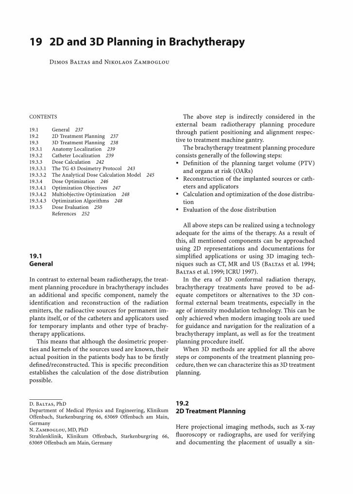
2D and 3D Planning in Brachytherapy 237

19 2D and 3D Planning in Brachytherapy

Dimos Baltas and Nikolaos Zamboglou

D. Baltas, PhDDepartment of Medical Physics and Engineering, Klinikum Offenbach, Starkenburgring 66, 63069 Offenbach am Main, GermanyN. Zamboglou, MD, PhDStrahlenklinik, Klinikum Offenbach, Starkenburgring 66, 63069 Offenbach am Main, Germany

19.1 General

In contrast to external beam radiotherapy, the treat-ment planning procedure in brachytherapy includes an additional and specifi c component, namely the identifi cation and reconstruction of the radiation emitters, the radioactive sources for permanent im-plants itself, or of the catheters and applicators used for temporary implants and other type of brachy-therapy applications.

This means that although the dosimetric proper-ties and kernels of the sources used are known, their actual position in the patients body has to be fi rstly defi ned/reconstructed. This is specifi c precondition establishes the calculation of the dose distribution possible.

The above step is indirectly considered in the external beam radiotherapy planning procedure through patient positioning and alignment respec-tive to treatment machine gantry.

The brachytherapy treatment planning procedure consists generally of the following steps:• Defi nition of the planning target volume (PTV)

and organs at risk (OARs)• Reconstruction of the implanted sources or cath-

eters and applicators• Calculation and optimization of the dose distribu-

tion• Evaluation of the dose distribution

All above steps can be realized using a technology adequate for the aims of the therapy. As a result of this, all mentioned components can be approached using 2D representations and documentations for simplifi ed applications or using 3D imaging tech-niques such as CT, MR and US (Baltas et al. 1994; Baltas et al. 1999; ICRU 1997).

In the era of 3D conformal radiation therapy, brachytherapy treatments have proved to be ad-equate competitors or alternatives to the 3D con-formal external beam treatments, especially in the age of intensity modulation technology. This can be only achieved when modern imaging tools are used for guidance and navigation for the realization of a brachytherapy implant, as well as for the treatment planning procedure itself.

When 3D methods are applied for all the above steps or components of the treatment planning pro-cedure, then we can characterize this as 3D treatment planning.

19.2 2D Treatment Planning

Here projectional imaging methods, such as X-ray fl uoroscopy or radiographs, are used for verifying and documenting the placement of usually a sin-

CONTENTS

19.1 General 23719.2 2D Treatment Planning 23719.3 3D Treatment Planning 23819.3.1 Anatomy Localization 23919.3.2 Catheter Localization 23919.3.3 Dose Calculation 24219.3.3.1 The TG 43 Dosimetry Protocol 24319.3.3.2 The Analytical Dose Calculation Model 24519.3.4 Dose Optimization 24619.3.4.1 Optimization Objectives 24719.3.4.2 Multiobjective Optimization 24819.3.4.3 Optimization Algorithms 24819.3.5 Dose Evaluation 250 References 252

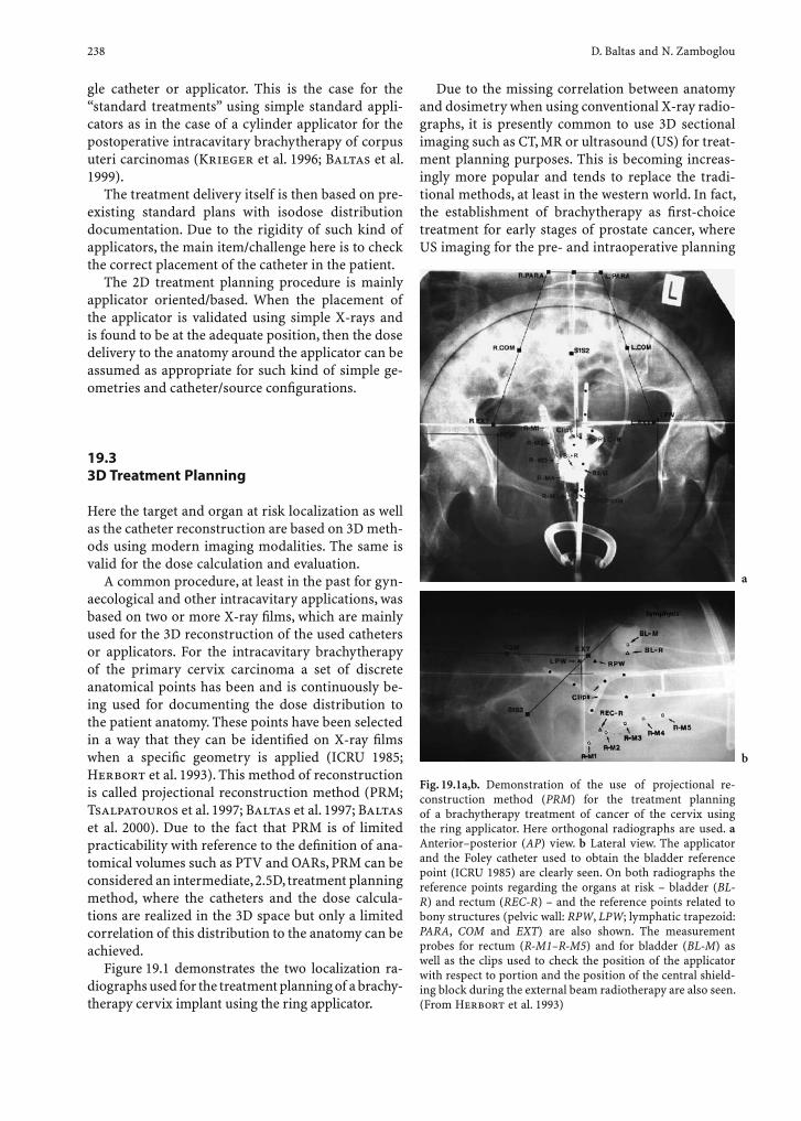
238 D. Baltas and N. Zamboglou

gle catheter or applicator. This is the case for the “standard treatments” using simple standard appli-cators as in the case of a cylinder applicator for the postoperative intracavitary brachytherapy of corpus uteri carcinomas (Krieger et al. 1996; Baltas et al. 1999).

The treatment delivery itself is then based on pre-existing standard plans with isodose distribution documentation. Due to the rigidity of such kind of applicators, the main item/challenge here is to check the correct placement of the catheter in the patient.

The 2D treatment planning procedure is mainly applicator oriented/based. When the placement of the applicator is validated using simple X-rays and is found to be at the adequate position, then the dose delivery to the anatomy around the applicator can be assumed as appropriate for such kind of simple ge-ometries and catheter/source confi gurations.

19.3 3D Treatment Planning

Here the target and organ at risk localization as well as the catheter reconstruction are based on 3D meth-ods using modern imaging modalities. The same is valid for the dose calculation and evaluation.

A common procedure, at least in the past for gyn-aecological and other intracavitary applications, was based on two or more X-ray fi lms, which are mainly used for the 3D reconstruction of the used catheters or applicators. For the intracavitary brachytherapy of the primary cervix carcinoma a set of discrete anatomical points has been and is continuously be-ing used for documenting the dose distribution to the patient anatomy. These points have been selected in a way that they can be identifi ed on X-ray fi lms when a specifi c geometry is applied (ICRU 1985; Herbort et al. 1993). This method of reconstruction is called projectional reconstruction method (PRM; Tsalpatouros et al. 1997; Baltas et al. 1997; Baltas et al. 2000). Due to the fact that PRM is of limited practicability with reference to the defi nition of ana-tomical volumes such as PTV and OARs, PRM can be considered an intermediate, 2.5D, treatment planning method, where the catheters and the dose calcula-tions are realized in the 3D space but only a limited correlation of this distribution to the anatomy can be achieved.

Figure 19.1 demonstrates the two localization ra-diographs used for the treatment planning of a brachy-therapy cervix implant using the ring applicator.

Due to the missing correlation between anatomy and dosimetry when using conventional X-ray radio-graphs, it is presently common to use 3D sectional imaging such as CT, MR or ultrasound (US) for treat-ment planning purposes. This is becoming increas-ingly more popular and tends to replace the tradi-tional methods, at least in the western world. In fact, the establishment of brachytherapy as fi rst-choice treatment for early stages of prostate cancer, where US imaging for the pre- and intraoperative planning

Fig. 19.1a,b. Demonstration of the use of projectional re-construction method (PRM) for the treatment planning of a brachytherapy treatment of cancer of the cervix using the ring applicator. Here orthogonal radiographs are used. a Anterior–posterior (AP) view. b Lateral view. The applicator and the Foley catheter used to obtain the bladder reference point (ICRU 1985) are clearly seen. On both radiographs the reference points regarding the organs at risk – bladder (BL-R) and rectum (REC-R) – and the reference points related to bony structures (pelvic wall: RPW, LPW; lymphatic trapezoid: PARA, COM and EXT) are also shown. The measurement probes for rectum (R-M1–R-M5) and for bladder (BL-M) as well as the clips used to check the position of the applicator with respect to portion and the position of the central shield-ing block during the external beam radiotherapy are also seen. (From Herbort et al. 1993)

b

a

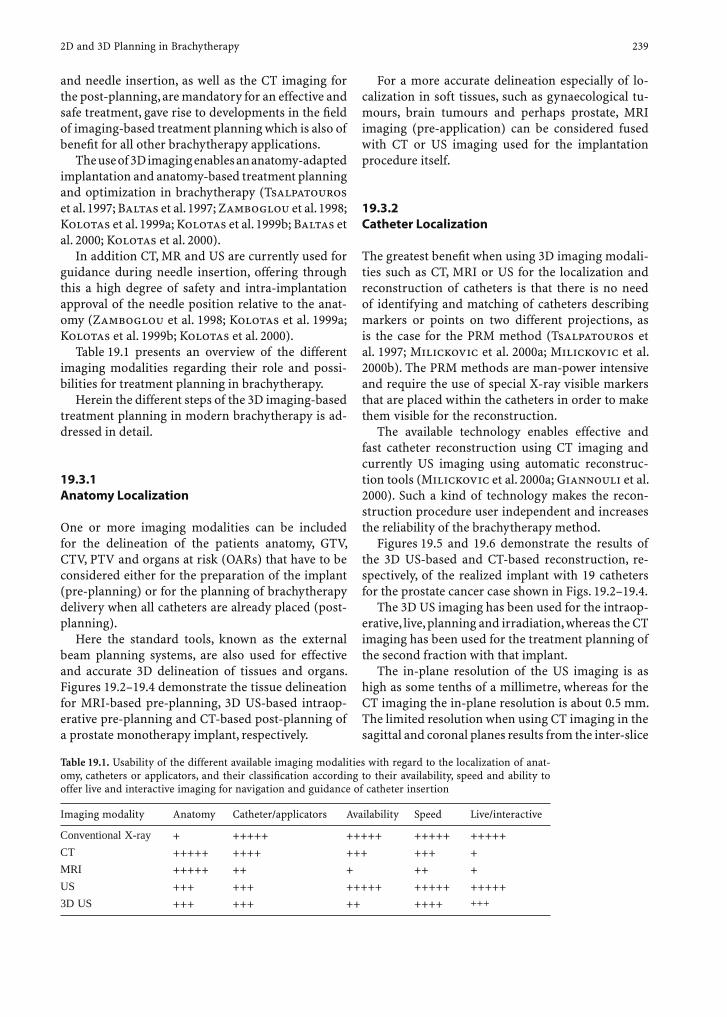
2D and 3D Planning in Brachytherapy 239

and needle insertion, as well as the CT imaging for the post-planning, are mandatory for an effective and safe treatment, gave rise to developments in the fi eld of imaging-based treatment planning which is also of benefi t for all other brachytherapy applications.

The use of 3D imaging enables an anatomy-adapted implantation and anatomy-based treatment planning and optimization in brachytherapy (Tsalpatouros et al. 1997; Baltas et al. 1997; Zamboglou et al. 1998; Kolotas et al. 1999a; Kolotas et al. 1999b; Baltas et al. 2000; Kolotas et al. 2000).

In addition CT, MR and US are currently used for guidance during needle insertion, offering through this a high degree of safety and intra-implantation approval of the needle position relative to the anat-omy (Zamboglou et al. 1998; Kolotas et al. 1999a; Kolotas et al. 1999b; Kolotas et al. 2000).

Table 19.1 presents an overview of the different imaging modalities regarding their role and possi-bilities for treatment planning in brachytherapy.

Herein the different steps of the 3D imaging-based treatment planning in modern brachytherapy is ad-dressed in detail.

19.3.1 Anatomy Localization

One or more imaging modalities can be included for the delineation of the patients anatomy, GTV, CTV, PTV and organs at risk (OARs) that have to be considered either for the preparation of the implant (pre-planning) or for the planning of brachytherapy delivery when all catheters are already placed (post-planning).

Here the standard tools, known as the external beam planning systems, are also used for effective and accurate 3D delineation of tissues and organs. Figures 19.2–19.4 demonstrate the tissue delineation for MRI-based pre-planning, 3D US-based intraop-erative pre-planning and CT-based post-planning of a prostate monotherapy implant, respectively.

For a more accurate delineation especially of lo-calization in soft tissues, such as gynaecological tu-mours, brain tumours and perhaps prostate, MRI imaging (pre-application) can be considered fused with CT or US imaging used for the implantation procedure itself.

19.3.2 Catheter Localization

The greatest benefi t when using 3D imaging modali-ties such as CT, MRI or US for the localization and reconstruction of catheters is that there is no need of identifying and matching of catheters describing markers or points on two different projections, as is the case for the PRM method (Tsalpatouros et al. 1997; Milickovic et al. 2000a; Milickovic et al. 2000b). The PRM methods are man-power intensive and require the use of special X-ray visible markers that are placed within the catheters in order to make them visible for the reconstruction.

The available technology enables effective and fast catheter reconstruction using CT imaging and currently US imaging using automatic reconstruc-tion tools (Milickovic et al. 2000a; Giannouli et al. 2000). Such a kind of technology makes the recon-struction procedure user independent and increases the reliability of the brachytherapy method.

Figures 19.5 and 19.6 demonstrate the results of the 3D US-based and CT-based reconstruction, re-spectively, of the realized implant with 19 catheters for the prostate cancer case shown in Figs. 19.2–19.4.

The 3D US imaging has been used for the intraop-erative, live, planning and irradiation, whereas the CT imaging has been used for the treatment planning of the second fraction with that implant.

The in-plane resolution of the US imaging is as high as some tenths of a millimetre, whereas for the CT imaging the in-plane resolution is about 0.5 mm. The limited resolution when using CT imaging in the sagittal and coronal planes results from the inter-slice

Table 19.1. Usability of the different available imaging modalities with regard to the localization of anat-omy, catheters or applicators, and their classifi cation according to their availability, speed and ability to offer live and interactive imaging for navigation and guidance of catheter insertion

Imaging modality Anatomy Catheter/applicators Availability Speed Live/interactive

Conventional X-ray + +++++ +++++ +++++ +++++CT +++++ ++++ +++ +++ +MRI +++++ ++ + ++ +US +++ +++ +++++ +++++ +++++3D US +++ +++ ++ ++++ +++

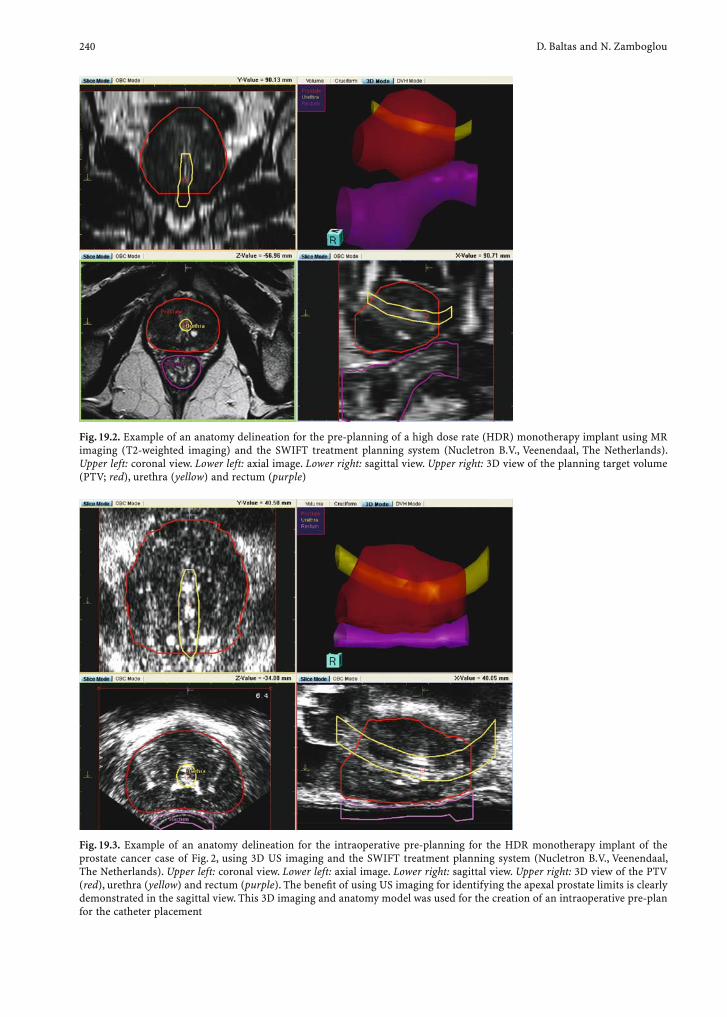
240 D. Baltas and N. Zamboglou

Fig. 19.2. Example of an anatomy delineation for the pre-planning of a high dose rate (HDR) monotherapy implant using MR imaging (T2-weighted imaging) and the SWIFT treatment planning system (Nucletron B.V., Veenendaal, The Netherlands). Upper left: coronal view. Lower left: axial image. Lower right: sagittal view. Upper right: 3D view of the planning target volume (PTV; red), urethra (yellow) and rectum (purple)

Fig. 19.3. Example of an anatomy delineation for the intraoperative pre-planning for the HDR monotherapy implant of the prostate cancer case of Fig. 2, using 3D US imaging and the SWIFT treatment planning system (Nucletron B.V., Veenendaal, The Netherlands). Upper left: coronal view. Lower left: axial image. Lower right: sagittal view. Upper right: 3D view of the PTV (red), urethra (yellow) and rectum (purple). The benefi t of using US imaging for identifying the apexal prostate limits is clearly demonstrated in the sagittal view. This 3D imaging and anatomy model was used for the creation of an intraoperative pre-plan for the catheter placement

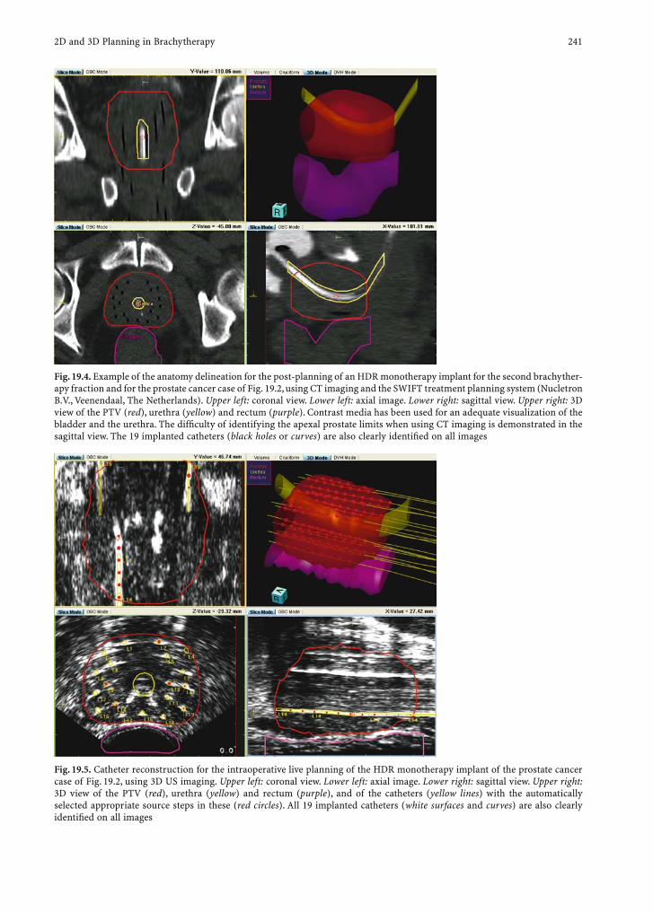
2D and 3D Planning in Brachytherapy 241

Fig. 19.4. Example of the anatomy delineation for the post-planning of an HDR monotherapy implant for the second brachyther-apy fraction and for the prostate cancer case of Fig. 19.2, using CT imaging and the SWIFT treatment planning system (Nucletron B.V., Veenendaal, The Netherlands). Upper left: coronal view. Lower left: axial image. Lower right: sagittal view. Upper right: 3D view of the PTV (red), urethra (yellow) and rectum (purple). Contrast media has been used for an adequate visualization of the bladder and the urethra. The diffi culty of identifying the apexal prostate limits when using CT imaging is demonstrated in the sagittal view. The 19 implanted catheters (black holes or curves) are also clearly identifi ed on all images

Fig. 19.5. Catheter reconstruction for the intraoperative live planning of the HDR monotherapy implant of the prostate cancer case of Fig. 19.2, using 3D US imaging. Upper left: coronal view. Lower left: axial image. Lower right: sagittal view. Upper right: 3D view of the PTV (red), urethra (yellow) and rectum (purple), and of the catheters (yellow lines) with the automatically selected appropriate source steps in these (red circles). All 19 implanted catheters (white surfaces and curves) are also clearly identifi ed on all images

242 D. Baltas and N. Zamboglou

distance. In the example of Figs. 19.4 and 19.6 this was 3.0 mm. Generally, the total accuracy that can be achieved with CT or MR imaging is half the slice thickness with the precondition that slice thickness equals the inter-slice distance (no gap). It is recom-mended to use for the reconstruction of not straight (metallic) catheters a slice thickness and inter-slice distance of 3 mm, achieving in this way an accuracy as high as 1.5 mm. When using axial MR imaging, then usually the longitudinal image distance is 5.0 mm re-sulting in an accuracy of 2.5 mm, which makes MRI for catheter reconstruction in several cases of limited interest. This can be overcome if non-axial MRI can be incorporated in the reconstruction procedure.

In contrast to CT, in 3D US imaging the inter-plane distance is as low as 1.0 mm (Figs. 19.3, 19.5), result-ing thus in an accuracy better than 1.0 mm (actually of ca. 0.5 mm). Another benefi t of US imaging for the reconstruction of catheters is the possibility to com-bine 3D volume reconstruction with live 2D imaging, offering in this way the possibility of an interactive reconstruction.

19.3.3 Dose Calculation

Although several national protocols exist for the dose calculation around brachytherapy sources, the protocol proposed and established by the American Association of Physicists in Medicine (AAPM), Task Group 43, and published in 1995 (Nath et al. 1995), has been widely accepted and builds the standard protocol that the majority of vendors of treatment planning systems in brachy-therapy are following. Even if this was primarily focused to low dose rate (LDR) sources (in the original publication it was explicitly mentioned that high activity sources and iridium wires were beyond the scope of that report), the TG 43 for-malism has been widely used and virtually inter-nationally accepted also for high dose rate (HDR) iridium sources used in remote afterloading sys-tems

The TG 43 formalism is a consistent, and a simple to implement, formalism based on a small number

Fig. 19.6. Catheter reconstruction for the post-operative planning for the second brachytherapy fraction and for the HDR monotherapy implant of the prostate cancer case of Fig. 19.2, using CT imaging. Upper left: coronal view. Lower left: axial im-age. Lower right: sagittal view. Upper right: 3D view of the PTV (red), urethra (yellow) and rectum (purple), and of the catheters (yellow lines) with the automatically selected appropriate source steps in these (red circles). All 19 implanted catheters (black holes and curves) are also clearly identifi ed on all images

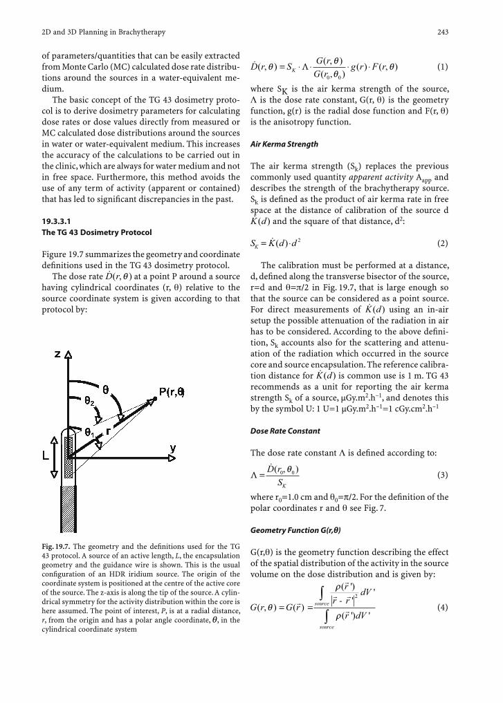
2D and 3D Planning in Brachytherapy 243

of parameters/quantities that can be easily extracted from Monte Carlo (MC) calculated dose rate distribu-tions around the sources in a water-equivalent me-dium.

The basic concept of the TG 43 dosimetry proto-col is to derive dosimetry parameters for calculating dose rates or dose values directly from measured or MC calculated dose distributions around the sources in water or water-equivalent medium. This increases the accuracy of the calculations to be carried out in the clinic, which are always for water medium and not in free space. Furthermore, this method avoids the use of any term of activity (apparent or contained) that has led to signifi cant discrepancies in the past.

19.3.3.1 The TG 43 Dosimetry Protocol

Figure 19.7 summarizes the geometry and coordinate defi nitions used in the TG 43 dosimetry protocol.

The dose rate &D r( , )θ at a point P around a source having cylindrical coordinates (r, ) relative to the source coordinate system is given according to that protocol by:

⋅ ⋅&D r S G rG r

g r F rK( , ) ( , )( , )

( ) ( , )θ θθ

θ= ⋅ ⋅Λ0 0

(1)

where SK is the air kerma strength of the source, is the dose rate constant, G(r, ) is the geometry

function, g(r) is the radial dose function and F(r, ) is the anisotropy function.

Air Kerma Strength

The air kerma strength (Sk) replaces the previous commonly used quantity apparent activity Aapp and describes the strength of the brachytherapy source. Sk is defi ned as the product of air kerma rate in free space at the distance of calibration of the source d &K d( ) and the square of that distance, d2:

S K d dK = ⋅& ( ) 2 (2)

The calibration must be performed at a distance, d, defi ned along the transverse bisector of the source, r=d and = /2 in Fig. 19.7, that is large enough so that the source can be considered as a point source. For direct measurements of &K d( ) using an in-air setup the possible attenuation of the radiation in air has to be considered. According to the above defi ni-tion, Sk accounts also for the scattering and attenu-ation of the radiation which occurred in the source core and source encapsulation. The reference calibra-tion distance for &K d( ) is common use is 1 m. TG 43 recommends as a unit for reporting the air kerma strength Sk of a source, µGy.m2.h–1, and denotes this by the symbol U: 1 U=1 µGy.m2.h–1=1 cGy.cm2.h–1

Dose Rate Constant

The dose rate constant is defi ned according to:

Λ =&D r

SK

( , )0 0θ (3)

where r0=1.0 cm and 0=π/2. For the defi nition of the polar coordinates r and see Fig. 7.

Geometry Function G(r,θ)

G(r, ) is the geometry function describing the effect of the spatial distribution of the activity in the source volume on the dose distribution and is given by:

G r G r

rr r

dV

r dVsource

source

( , ) ( )

( ')'

'

( ') 'θ

ρ

ρ= =

−∫

∫r

r

r r

r

2

(4)

Fig. 19.7. The geometry and the defi nitions used for the TG 43 protocol. A source of an active length, L, the encapsulation geometry and the guidance wire is shown. This is the usual confi guration of an HDR iridium source. The origin of the coordinate system is positioned at the centre of the active core of the source. The z-axis is along the tip of the source. A cylin-drical symmetry for the activity distribution within the core is here assumed. The point of interest, P, is at a radial distance, r, from the origin and has a polar angle coordinate, θ, in the cylindrical coordinate system

244 D. Baltas and N. Zamboglou

where (r’) is the activity per unit volume at a point r’ inside the source and dV’ is an infi nitesimal vol-ume element located at the same position. This factor reduces to:

G r G rr

( , ) ( )q = = 12 for a point source (5)

G rL r

( , )sin

θ θ θθ

= −⋅ ⋅

2 1 for a fi nite line source (6)

Here L is the active length of the source and the angles 1 and 2 are illustrated in Fig. 19.7.

Reference Point of Dose Calculations

The reference point is that for the formalism chosen to be the point lying on the transverse bisector of the source at a distance of 1 cm from its centre: expressed in polar coordinates as defi ned in Fig. 19.7, i.e. (r0,

0)=(1cm, /2).

Radial Dose Function

g(r) is the radial dose function and is defi ned as:

g r G rG r

D rD r

( ) ( , )( , )

( , )( , )

=⎡

⎣⎢

⎤

⎦⎥ ⋅

⎡

⎣⎢

⎤

⎦⎥0 0

0

0

0 0

θθ

θθ

&

& (7)

Anisotropy Function

Finally, F(r, ) is the anisotropy function defi ned as:

F r G rG r

D rD r

( , ) ( , )( , )

( , )( , )

θ θθ

θθ

=⎡

⎣⎢

⎤

⎦⎥ ⋅

⎡

⎣⎢

⎤

⎦⎥0

0

&

& (8)

Anisotropy Factor

Because of the diffi culty in determining the orienta-tion of the implanted seeds, post-implant dosimetry for low dose rate permanent implants is based on the point source approximation using the anisotropy factor an(r):

⋅ ⋅φθ

θ θ θπ

an rD r

D r d( )( , )

( , ) sin=⋅

⎡

⎣⎢

⎤

⎦⎥ ⋅ =∫

12 0 0

&&

θ θθG r( , )⋅

⎡

⎣⎢

⎤12 0 ⎦⎦

⎥ ⋅ ⋅ ⋅ ⋅∫ F r G r d( , ) ( , ) sinθ θπ

0 (9)

This is uncommon for the case of HDR iridium-192-based brachytherapy where the TG 43 formalism as given in Eq. (1) with the line source approximation described in Eq. (6) is used.

Anisotropy Constant

Using a 1/r2 weighted-average of anisotropy factors, for r>1 cm, the distance independent anisotropy fac-tor an is calculated using the equation:

ϕ

ϕ

an

an i

i2

i

i2

i

(r )r1r

=∑

∑ (10)

In the literature the TG 43 parameter values and functions for the common used seeds or HDR irid-ium sources can be found.

Recently AAPM has updated the TG 43 protocol for low-activity seeds (Rivard et al. 2004), where it is recommended to use separately radial dose functions g(r) and anisotropy functions F(r, ) as well as anisot-ropy factors an(r) and anisotropy constants an in dependence on the geometry factor is used; point (see Eq. (5)) or line (see Eq. (6)) source approxima-tion. This report contains the corresponding tables for all factors and functions for the most common seeds according to the new formulation.

Although the TG 43 formalism offers a stable plat-form for calculation of dose or dose rate distributions in brachytherapy, it can be easily seen from Eq. (1) that the TG 43 formalism is actually a 2D model.

Tissue inhomogeneities and bounded geometries are not considered by this formalism. The effects of the presence of inhomogeneities and the variable dimensions of patient-specifi c anatomy are ignored. The MC simulation would be the only accurate solu-tion to the aforementioned defi ciencies based on ac-tual patient anatomical data. That is, however, still too time-consuming to be incorporated in a clinical envi-ronment in spite of promising correlated simulation techniques (Hedtjärn et al. 2002); therefore, kernel superposition methods (Williamson and Baker 1991; Carlsson and Ahnesjö 2000; Carlsson Tedgren and Ahnesjö 2003) and analytical models (Williamson et al. 1993; Kirov and Williamson 1997; Daskalov et al. 1998) have been employed and tested in a variety of geometries, thus opening the way of handling tissue and shielding material inho-mogeneities and bounded patient geometries.

A simpler analytical dosimetry model (Anagnostopoulos et al. 2003) based on the pri-mary and scatter separation technique (Russell and Ahnesjö 1996; Williamson 1996) was published and evaluated in patient-equivalent phantom ge-ometries (Pantelis et al. 2004; Anagnostopoulos et al. 2004). The kernel superposition as well as the analytical dose calculation models announce in this

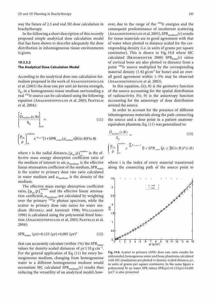
2D and 3D Planning in Brachytherapy 245

way the future of 2.5 and real 3D dose calculation in brachytherapy.

In the following a short description of this recently proposed simple analytical dose calculation model that has been shown to describe adequately the dose distribution in inhomogeneous tissue environments is given.

19.3.3.2 The Analytical Dose Calculation Model

According to the analytical dose rate calculation for-malism proposed in the work of Anagnostopoulos et al. (2003) the dose rate per unit air kerma strength, SK, in a homogeneous tissue medium surrounding a real 192Ir source can be calculated using the following equation (Anagnostopoulos et al. 2003; Pantelis et al. 2004):

D rS

medium

Kreal

•⎡

⎣

⎢⎢

⎤

⎦

⎥⎥

=( , )θ

(11)

( ) ) (( ) r Fρ θ( ,r me S1− ⋅en

air

mediumrmed

⎛

⎝⎜

⎞

⎠⎟ +µ

ρµ PR r G rwate edium , )θ

where r is the radial distance, ( )en air

mediumµ ρ/ is the ef-fective mass energy absorption coeffi cient ratio of the medium of interest to air, medium is the effective linear attenuation coeffi cient of the medium, SPRwater is the scatter to primary dose rate ratio calculated in water medium and medium is the density of the medium.

The effective mass energy absorption coeffi cient ratio, ( )en air

mediumµ ρ/ and the effective linear attenua-tion coeffi cient, medium, are calculated by weighting over the primary 192Ir photon spectrum, while the scatter to primary dose rate ratios for water me-dium (Russell and Ahnesjö 1996; Williamson 1996) is calculated using the polynomial fi tted func-tion (Anagnostopoulos et al. 2003; Pantelis et al. 2004):

SPRwater ( r)=0.123 ( r)+0.005 ( r)2 (12)

that can accurately calculate (within 1%) the SPRwater values for density-scaled distances of r ≤ 10 g cm–2. For the general application of Eq. (11) for every ho-mogeneous medium, changing from homogeneous water to a different homogeneous medium would necessitate MC calculated SPRmedium(r) results thus reducing the versatility of an analytical model; how-

ever, due to the range of the 192Ir energies and the consequent predominance of incoherent scattering (Anagnostopoulos et al. 2003), SPRmedium(r) results for tissue materials are in good agreement with that of water when plotted vs distance scaled for the cor-responding density (i.e. in units of grams per square centimetre). This is shown in Fig. 19.8 where MC calculated (Briesmeister 2000) SPRbone(r) ratios of cortical bone are also plotted vs distance from a point 192Ir source multiplied by the corresponding material density (1.92 g/cm3 for bone) and an over-all good agreement within 1–5% may be observed (Anagnostopoulos et al. 2003).

In this equation, G(r, ) is the geometry function of the source accounting for the spatial distribution of radioactivity. F(r, ) is the anisotropy function accounting for the anisotropy of dose distribution around the source.

In order to account for the presence of different inhomogeneous materials along the path connecting the source and a dose point in a patient anatomy-equivalent phantom, Eq. (11) was generalized to:

),( θ

SrD

K

medium =&

(13)

( )( ) ),(),( .1.

θθρρµ µ

rFrGrSPRe iiwater

rmedium

air

en iiimedium

+∑

⎟⎟⎠

⎞⎜⎜⎝

⎛ −

where i is the index of every material transversed along the connecting path of the source point to

pr (g/cm2)

SPR

waterbone

Fig. 19.8. Scatter to primary (SPR) dose rate ratio results for unbounded, homogenous water and bone phantoms calculated with MC simulations are plotted vs density-scaled distance, r, in units of grams per square centimetre. In the same fi gure a polynomial fi t on water SPR values SPR( r)=0.123( r)+0.005( r)2 is also presented

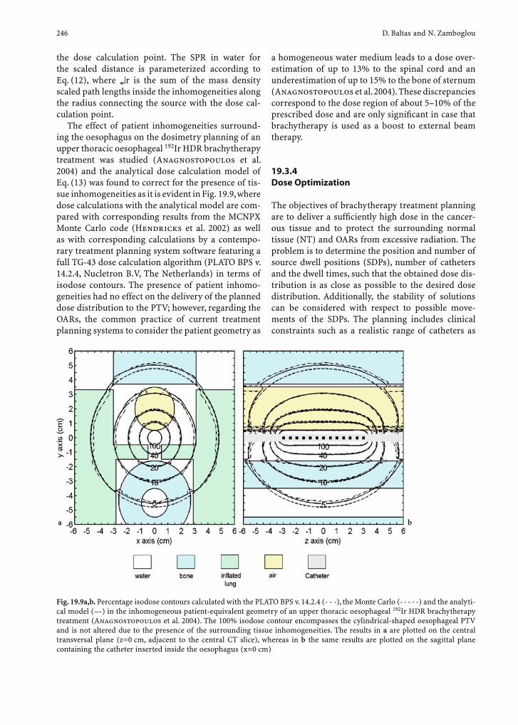
246 D. Baltas and N. Zamboglou

the dose calculation point. The SPR in water for the scaled distance is parameterized according to Eq. (12), where r is the sum of the mass density scaled path lengths inside the inhomogeneities along the radius connecting the source with the dose cal-culation point.

The effect of patient inhomogeneities surround-ing the oesophagus on the dosimetry planning of an upper thoracic oesophageal 192Ir HDR brachytherapy treatment was studied (Anagnostopoulos et al. 2004) and the analytical dose calculation model of Eq. (13) was found to correct for the presence of tis-sue inhomogeneities as it is evident in Fig. 19.9, where dose calculations with the analytical model are com-pared with corresponding results from the MCNPX Monte Carlo code (Hendricks et al. 2002) as well as with corresponding calculations by a contempo-rary treatment planning system software featuring a full TG-43 dose calculation algorithm (PLATO BPS v. 14.2.4, Nucletron B.V, The Netherlands) in terms of isodose contours. The presence of patient inhomo-geneities had no effect on the delivery of the planned dose distribution to the PTV; however, regarding the OARs, the common practice of current treatment planning systems to consider the patient geometry as

a homogeneous water medium leads to a dose over-estimation of up to 13% to the spinal cord and an underestimation of up to 15% to the bone of sternum (Anagnostopoulos et al. 2004). These discrepancies correspond to the dose region of about 5–10% of the prescribed dose and are only signifi cant in case that brachytherapy is used as a boost to external beam therapy.

19.3.4 Dose Optimization

The objectives of brachytherapy treatment planning are to deliver a suffi ciently high dose in the cancer-ous tissue and to protect the surrounding normal tissue (NT) and OARs from excessive radiation. The problem is to determine the position and number of source dwell positions (SDPs), number of catheters and the dwell times, such that the obtained dose dis-tribution is as close as possible to the desired dose distribution. Additionally, the stability of solutions can be considered with respect to possible move-ments of the SDPs. The planning includes clinical constraints such as a realistic range of catheters as

Fig. 19.9a,b. Percentage isodose contours calculated with the PLATO BPS v. 14.2.4 (- - -), the Monte Carlo (- · - · -) and the analyti-cal model (—) in the inhomogeneous patient-equivalent geometry of an upper thoracic oesophageal 192Ir HDR brachytherapy treatment (Anagnostopoulos et al. 2004). The 100% isodose contour encompasses the cylindrical-shaped oesophageal PTV and is not altered due to the presence of the surrounding tissue inhomogeneities. The results in a are plotted on the central transversal plane (z=0 cm, adjacent to the central CT slice), whereas in b the same results are plotted on the sagittal plane containing the catheter inserted inside the oesophagus (x=0 cm)

a b

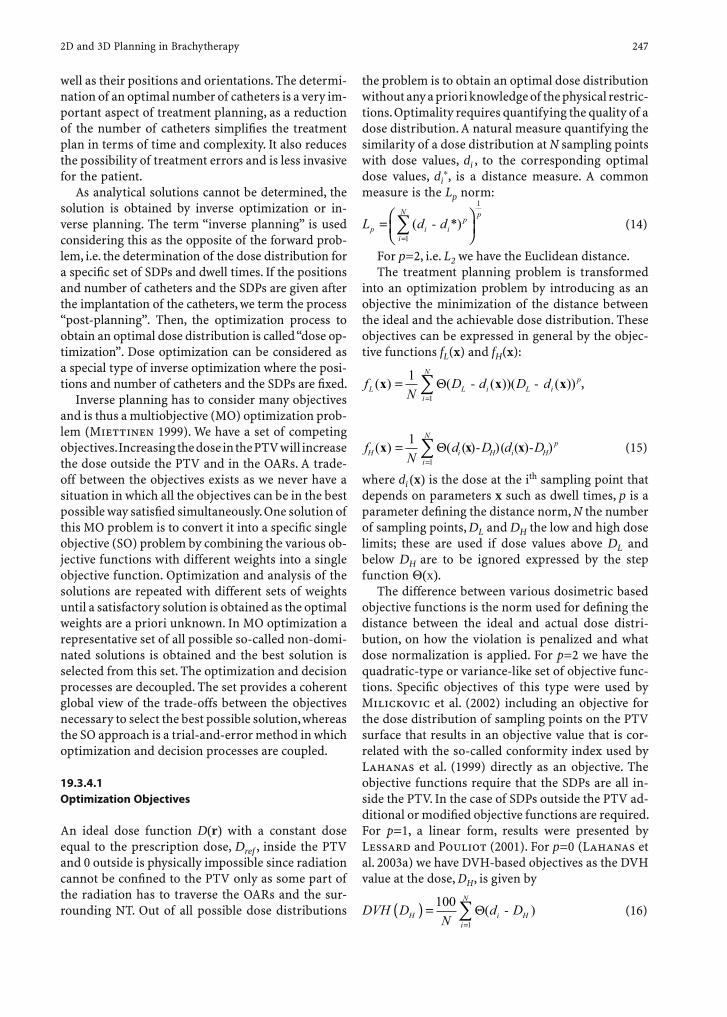
2D and 3D Planning in Brachytherapy 247

well as their positions and orientations. The determi-nation of an optimal number of catheters is a very im-portant aspect of treatment planning, as a reduction of the number of catheters simplifi es the treatment plan in terms of time and complexity. It also reduces the possibility of treatment errors and is less invasive for the patient.

As analytical solutions cannot be determined, the solution is obtained by inverse optimization or in-verse planning. The term “inverse planning” is used considering this as the opposite of the forward prob-lem, i.e. the determination of the dose distribution for a specifi c set of SDPs and dwell times. If the positions and number of catheters and the SDPs are given after the implantation of the catheters, we term the process “post-planning”. Then, the optimization process to obtain an optimal dose distribution is called “dose op-timization”. Dose optimization can be considered as a special type of inverse optimization where the posi-tions and number of catheters and the SDPs are fi xed.

Inverse planning has to consider many objectives and is thus a multiobjective (MO) optimization prob-lem (Miettinen 1999). We have a set of competing objectives. Increasing the dose in the PTV will increase the dose outside the PTV and in the OARs. A trade-off between the objectives exists as we never have a situation in which all the objectives can be in the best possible way satisfi ed simultaneously. One solution of this MO problem is to convert it into a specifi c single objective (SO) problem by combining the various ob-jective functions with different weights into a single objective function. Optimization and analysis of the solutions are repeated with different sets of weights until a satisfactory solution is obtained as the optimal weights are a priori unknown. In MO optimization a representative set of all possible so-called non-domi-nated solutions is obtained and the best solution is selected from this set. The optimization and decision processes are decoupled. The set provides a coherent global view of the trade-offs between the objectives necessary to select the best possible solution, whereas the SO approach is a trial-and-error method in which optimization and decision processes are coupled.

19.3.4.1 Optimization Objectives

An ideal dose function D(r) with a constant dose equal to the prescription dose, Dref , inside the PTV and 0 outside is physically impossible since radiation cannot be confi ned to the PTV only as some part of the radiation has to traverse the OARs and the sur-rounding NT. Out of all possible dose distributions

the problem is to obtain an optimal dose distribution without any a priori knowledge of the physical restric-tions. Optimality requires quantifying the quality of a dose distribution. A natural measure quantifying the similarity of a dose distribution at N sampling points with dose values, di , to the corresponding optimal dose values, di

�, is a distance measure. A common measure is the Lp norm:

L d dp i ip

i

N p= −⎛

⎝⎜⎞⎠⎟=

∑ ( *)1

1

(14)

For p=2, i.e. L2 we have the Euclidean distance.The treatment planning problem is transformed

into an optimization problem by introducing as an objective the minimization of the distance between the ideal and the achievable dose distribution. These objectives can be expressed in general by the objec-tive functions fL(x) and fH(x):

fN

D d D dL L i L ip

i

N

( ) ( ( ))( ( ))x x x= − −=∑1

1Θ ,

x xd Dd D( (x =Hf N H i Hp

i

N

( ) ) ( ) )−=∑1

1Θ i − )( (15)

where di (x) is the dose at the ith sampling point that depends on parameters x such as dwell times, p is a parameter defi ning the distance norm, N the number of sampling points, DL and DH the low and high dose limits; these are used if dose values above DL and below DH are to be ignored expressed by the step function (x).

The difference between various dosimetric based objective functions is the norm used for defi ning the distance between the ideal and actual dose distri-bution, on how the violation is penalized and what dose normalization is applied. For p=2 we have the quadratic-type or variance-like set of objective func-tions. Specifi c objectives of this type were used by Milickovic et al. (2002) including an objective for the dose distribution of sampling points on the PTV surface that results in an objective value that is cor-related with the so-called conformity index used by Lahanas et al. (1999) directly as an objective. The objective functions require that the SDPs are all in-side the PTV. In the case of SDPs outside the PTV ad-ditional or modifi ed objective functions are required. For p=1, a linear form, results were presented by Lessard and Pouliot (2001). For p=0 (Lahanas et al. 2003a) we have DVH-based objectives as the DVH value at the dose, DH , is given by

DVH DN

d DH i Hi

N

( ) = −=∑100

1Θ( ) (16)

248 D. Baltas and N. Zamboglou

The benefi t in this case is that the objective values are easier to interpret than for other objective func-tions, although different dose distributions could produce the same objective values, as the dose dis-tributions are only required to satisfy some integral properties. In this case gradient-based optimization algorithms cannot be used for dose optimization.

Dose-volume histogram specifying constraints for a clinically acceptable dose distribution can be in-cluded in the optimization (constraint dose optimi-zation). Such constraints could specify upper bounds for the fraction of the volume of a region that can accept a dose larger than a specifi c level, or a lower bound for the fraction that should have a dose at least larger than a specifi c value.

There are physical limitations of what dose dis-tributions can be obtained for a specifi c number of catheters and number of SDPs. The solutions ob-tained by inverse planning depend also on the used set of objective functions. The closer the dose distri-butions of these solutions are to the physically pos-sible optimal solution, the better the set of objective functions is.

19.3.4.2 Multiobjective Optimization

For MO optimization with M objectives we have a vector objective function f=(f1(x),...,fM(x)). In gen-eral, some of the individual objectives will be in con-fl ict with others, and some will have to be minimized while others are maximized. The MO optimization problem can now be defi ned as the problem to fi nd the vector x=(x1,x2,...,xN), i.e. solution which opti-mizes the vector function f. Normally, we never have a situation in which all the fi(x) values are optimal for a common point x. We therefore have to establish cer-tain criteria to determine what would be considered an optimal solution. One interpretation of the term optimum in MO optimization is the Pareto optimum (Miettinen 1999).

A solution x1 dominates a solution x2 if and only if the two following conditions are true:1. x1 is no worse than x2 in all objectives, i.e. fj(x 1)

fj(x 2) j=1,…,M.2. x1 is strictly better than x2 in at least one objective,

i.e. fj(x1) < fj(x2) for at least one j {1,…,M}.

We assume, without loss of generality, that this is a minimization problem. x1 is said to be non-dominated by x2 or x1 is non-inferior to x2 and x2 is dominated by x1. Among a set of solutions P, the non-dominated set of solutions P’ are those that are not dominated by

any other member of the set P. When the set P is the entire feasible search space then the set P’ is called the “global Pareto optimal set”. If for every member x of a set P there exists no solution in the neighbour-hood of x, then the solutions of P form a local Pareto optimal set. The image f(x) of the Pareto optimal set is called the “Pareto front”. The Pareto optimal set is defi ned in the parameter space, whereas the Pareto front is defi ned in the objective space.

19.3.4.3 Optimization Algorithms

The optimization algorithm used in brachytherapy planning depends on the selected set of objective functions. In the presence of local function minima deterministic algorithms may not work well. For vari-ance-based objectives gradient-based optimization algorithms guided by gradient information can be used for post-planning and the solutions obtained are global optimal (Lahanas et al. 2003b). It is also pos-sible to use special calculation methods (Lahanas and Baltas 2003) to perform a fast MO optimization in which the optimization is repeated with different uniform distributed sets of weights until a represen-tative set of non-dominated solutions is obtained. For MO inverse planning with other objectives functions which consider the problem of the optimal position and number of catheters to be used for specifi c MO hybrid evolutionary algorithms combine the power of effi ciency of deterministic algorithms with the parallel character nature of evolutionary algorithms with the aim of obtaining fast a representative set of Pareto optimal solutions.

Evolutionary algorithm (EA) is a collective term for all variants of probabilistic optimization algo-rithms that are inspired by Darwinian evolution. A genetic algorithm (GA) is a variant of EA, which, in analogy to the biological DNA alphabet, operates on strings which are usually bit strings of constant length. The string corresponds to the genotype of the individual. Usually, a GA has the following com-ponents:• A representation of potential solutions to the

problem• A method to create an initial population of poten-

tial solutions• An evaluation function that plays the role of the

environment, rating solutions in terms of their fi t-ness (expressed by a fi tness function, in principle an objective function)

• Genetic operators that alter the composition of the population members of the next generation

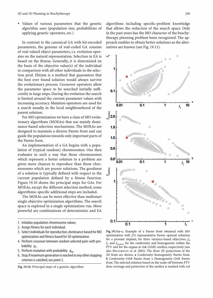
2D and 3D Planning in Brachytherapy 249

• Values of various parameters that the genetic algorithm uses (population size, probabilities of applying genetic operators, etc.)

In contrast to the canonical GA with bit-encoded parameters, the genome of real-coded GA consists of real-valued object parameters, i.e. evolution oper-ates on the natural representation. Selection in EA is based on the fi tness. Generally, it is determined on the basis of the objective value(s) of the individual in comparison with all other individuals in the selec-tion pool. Elitism is a method that guarantees that the best ever found solution would always survive the evolutionary process. Crossover operators allow the parameter space to be searched initially suffi -ciently in large steps. During the evolution the search is limited around the current parameter values with increasing accuracy. Mutation operators are used for a search usually in the local neighbourhood of the parent solution.

For MO optimization we have a class of MO evolu-tionary algorithms (MOEAs) that use mainly domi-nance-based selection mechanisms. The MOEAs are designed to maintain a diverse Pareto front and can guide the population towards only important parts of the Pareto front.

An implementation of a GA begins with a popu-lation of (typical random) chromosomes. One then evaluates in such a way that those chromosomes which represent a better solution to a problem are given more chances to reproduce than those chro-mosomes which are poorer solutions. The goodness of a solution is typically defi ned with respect to the current population defi ned by a fi tness function. Figure 19.10 shows the principal steps for GAs. For MOEAs, except the different selection method, some algorithmic-specifi c additional steps are included.

The MOEAs can be more effective than multistart single objective optimization algorithms. The search space is explored in a single optimization run. More powerful are combinations of deterministic and EA

algorithms including specifi c-problem knowledge that allows the reduction of the search space. Only in the past years has the MO character of the brachy-therapy planning problem been recognized. The ap-proach enables to obtain better solutions as the alter-natives are known (see Fig. 19.11).

fSf V

fS

f Uret

hra

fV

f Uret

hra

a

c

b

Fig. 19.11a–c. Example of a Pareto front obtained with MO optimization with 231 representative Pareto optimal solutions for a prostate implant, for three variance-based objectives, fS, fV and fUrethra for the conformity and homogeneity within the PTV and for the organs at risk (OAR) urethra, respectively (see also Milickovic et al. 2002). The three 2D projections of the 3D front are shown. a Conformity–homogeneity Pareto front. b Conformity–OAR Pareto front. c Homogeneity–OAR Pareto front. The selected solution based on the trade-off between PTV dose coverage and protection of the urethra is marked with red

1. Initialize population chromosome values.2. Assign fi tness for each individual. 3. Select individuals for reproduction, dominance based for MO optimization and fi tness based for SO optimization.4. Perform crossover between random selected pairs with pro- bability pC.5. Perform mutation with probability pM.6. Stop. If maximum generation is reached or any other stopping criterion is satisfi ed, see point 2.

Fig. 19.10. Principal steps of a genetic algorithm

250 D. Baltas and N. Zamboglou

Figure 19.12 demonstrates the results of a multi-objective optimization for a prostate monotherapy implant using the variance-based objectives: confor-mity and homogeneity for PTV; OAR urethra with a dose limit (critical dose, DH, value for the fH objective in Eq. (15)) of 125%; and OAR rectum with a dose limit (critical dose, DH, value for the fH objective in Eq. (15)) of 85% of the reference dose (100%).

The multiobjectivity of the anatomy-based op-timization and the need of decision tools is clearly demonstrated in Fig. 19.12.

19.3.5 Dose Evaluation

There have been several concepts and parameters defi ned and proposed for the evaluation of the 3D dose distribution in brachytherapy.

ICRU report 58 (ICRU 1997) offers an extended summary of the classical parameters that could be used for evaluating the dose distribution, but it is mainly focused on the system-based treatment plan-ning in interstitial brachytherapy. This report, on the

a

c

b

d

Fig. 19.12a–d. Results of the multi-objective optimization for a prostate HDR monotherapy implant with 15 needles using the SWIFT treatment planning system (Nucletron B.V., Veenendaal, The Netherlands). a A 3D view of the PTV (red), urethra (yellow) and rectum (light brown), and of the catheters (yellow lines) with the selected appropriate source steps in these (red circles). b Representative set of 84 alternative solutions when using the PTV conformity, PTV homogeneity, urethra and rectum as OAR objectives. The dose volume histograms for prostate (PTV) and urethra (OAR) demonstrate a very spread distribution. c The solution having the highest D90 value for prostate (curves at the right) compared with an alternative solution (curves at the left). The arrows demonstrate the shifts of the curves at the left. Dmin for prostate remains unchanged. The homogeneity in prostate volume, the DVH for the urethra and the DVH for the rectum are signifi cantly improved where the D90 for prostate is reduced insignifi cantly and only by 1.5%. d The solution having the highest coverage for the prostate, V100 (curves at the right), compared with the solution having the maximum conformity value (curves at the left). The arrows demonstrate the shifts of the curves to the left. Here the signifi cant improvement of the DVHs for the OARs urethra and rectum could be achieved at the expense of the dose distribution in the PTV (prostate). There is a reduction in the coverage, V100, of 6%, a reduction of the D90 value of 6.5% and a reduction of the minimum dose in PTV of 14%

2D and 3D Planning in Brachytherapy 251

other hand, introduces for the fi rst time anatomy-ori-ented parameters for evaluation as well as the volume defi nitions as already known in the external beam treatment planning: gross tumour volume (GTV); clinical target volume (CTV); planning target volume (PTV); and treated volume (TV).

In this report it is recommended to use the mini-mum target dose (MTD) defi ned as the minimum dose at the periphery of CTV and the mean central dose (MCD) that is taken as the arithmetic mean of the local minimum doses between sources or cathe-ters in the central plane for reporting and evaluating. The latest is according to the Paris system of dosim-etry in interstitial low dose rate (LDR) brachytherapy. Finally, the high dose volume, defi ned as the volumes encompassed by the isodose corresponding to 150% of the MCD, and the low dose volume, defi ned as the volume within the CTV, encompassed by the 90% iso-dose value, are considered.

In the past, efforts have been made for establishing some parameters or fi gures to describe the homoge-neity of the dose distribution in brachytherapy; all of these have been based on the absence of an ana-tomical dose calculation space. In other words, these efforts have considered the dose distribution sim-ply around the catheters. The method that found a wide application, at least in the fi eld of low-dose-rate brachytherapy, is that of natural dose volume histo-gram (NDVH) introduced by Anderson (Anderson 1986).

Currently published recommendations (Ash et al. 2000; Nag et al. 1999; Nag et al. 2001; Pötter et al. 2002) proposed DVH-based parameters (cumulative DVHs) for the evaluation and documentation of the dose distribution (see below).

PTV-Oriented Parameters

D100: the dose that covers 100% of the PTV volume, which is exactly the MTD proposed by ICRU report 58, if we assume that CTV equals PTV for brachytherapy

D90: the dose that covers 90% of the PTV volumeV100: the percentage of the PTV volume that has

received at least the prescribed dose, which is set to 100%.

V150: the volume, normally the PTV volume, that has received at least 150% of the prescribed dose

The defi nition of these parameters is graphically shown in Fig. 19.13. Statistical values, such as the mean dose value (Dmean) and the standard deviation of the dose value distribution in the PTV, can also be used.

OAR-Oriented Parameters

For the OARs there are not widely established dosi-metric parameters. The only exception are the values considered to be representative for the irradiation of bladder and rectum for the primary intracavitary brachytherapy of the cervix carcinoma as proposed by ICRU 38 (ICRU 1985; Pötter et al. 2002).

Pötter et al. (2002) propose to use the maximum dose for the OARs, at least for the case of primary intracavitary brachytherapy of the cervix carcinoma, where the maximum doses are considered to be the doses received in a volume of at least 2 and 5 cm3 for bladder and rectum, respectively.

Furthermore, die D10, defi ned as the highest dose covering 10% of the OAR volume, is commonly used for the interstitial brachytherapy of prostate cancer for documenting the dose distribution in the related OARs urethra, rectum and bladder.

The Conformal Index

Baltas et al. (1998) has introduced a utility function as a measure of the implant quality, the conformal index (COIN), which has been later expanded to in-clude OARs (Milickovic et al. 2002). The COIN takes into account patient anatomy, both of the PTV, sur-rounding normal tissue (NT) and OARs. The COIN for the reference dose value, Dref (prescribed dose), is defi ned as:

= ◊ ◊COIN c c c1 2 3 (17)

Fig. 19.13. Graphical demonstration of the defi nition of the D100, D90, V100 and V150 dosimetric parameters for an im-aging-based 3D brachytherapy treatment planning based on the cumulative dose volume histogram of PTV

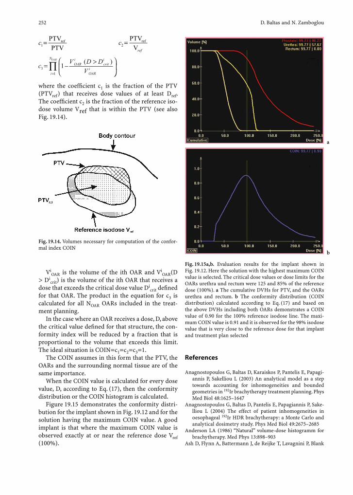
252 D. Baltas and N. Zamboglou

c1=PTVPTV

ref

c

ref2

refPTVV

=

where the coeffi cient c1 is the fraction of the PTV (PTVref) that receives dose values of at least Dref. The coeffi cient c2 is the fraction of the reference iso-dose volume Vref that is within the PTV (see also Fig. 19.14).

References

Anagnostopoulos G, Baltas D, Karaiskos P, Pantelis E, Papagi-annis P, Sakelliou L (2003) An analytical model as a step towards accounting for inhomogeneities and bounded geometries in 192Ir brachytherapy treatment planning. Phys Med Biol 48:1625–1647

Anagnostopoulos G, Baltas D, Pantelis E, Papagiannis P, Sake-lliou L (2004) The effect of patient inhomogeneities in oesophageal 192Ir HDR brachytherapy: a Monte Carlo and analytical dosimetry study. Phys Med Biol 49:2675–2685

Anderson LA (1986) “Natural” volume-dose histogramm for brachytherapy. Med Phys 13:898–903

Ash D, Flynn A, Battermann J, de Reijke T, Lavagnini P, Blank

Fig. 19.14. Volumes necessary for computation of the confor-mal index COIN

a

b

ViOAR is the volume of the ith OAR and Vi

OAR(D > Di

crit) is the volume of the ith OAR that receives a dose that exceeds the critical dose value Di

crit defi ned for that OAR. The product in the equation for c3 is calculated for all NOAR OARs included in the treat-ment planning.

In the case where an OAR receives a dose, D, above the critical value defi ned for that structure, the con-formity index will be reduced by a fraction that is proportional to the volume that exceeds this limit. The ideal situation is COIN=c1=c2=c3=1.

The COIN assumes in this form that the PTV, the OARs and the surrounding normal tissue are of the same importance.

When the COIN value is calculated for every dose value, D, according to Eq. (17), then the conformity distribution or the COIN histogram is calculated.

Figure 19.15 demonstrates the conformity distri-bution for the implant shown in Fig. 19.12 and for the solution having the maximum COIN value. A good implant is that where the maximum COIN value is observed exactly at or near the reference dose Vref (100%).

Fig. 19.15a,b. Evaluation results for the implant shown in Fig. 19.12. Here the solution with the highest maximum COIN value is selected. The critical dose values or dose limits for the OARs urethra und rectum were 125 and 85% of the reference dose (100%). a The cumulative DVHs for PTV, and the OARs urethra and rectum. b The conformity distribution (COIN distribution) calculated according to Eq. (17) and based on the above DVHs including both OARs demonstrates a COIN value of 0.90 for the 100% reference isodose line. The maxi-mum COIN value is 0.91 and it is observed for the 98% isodose value that is very close to the reference dose for that implant and treatment plan selected

2D and 3D Planning in Brachytherapy 253

L (2000) ESTRO/EAU/EORTC recommendations on per-manent seed implantation for localized prostate cancer. Radiother Oncol 57:315–321

Baltas D, Lapukins Z, Dotzel W, Herbort K, Voith C, Lietz C, Filbry E, Kober B (1994) Review of treatment of oesopha-geal cancer with special reference to Darmstadt experience. In: Bruggmoser G, Mould RF (eds) Brachytherapy review, Freiburg Oncology Series monograph no. 1. Proc German Brachytherapy Conference, Freiburg, pp 244–270

Baltas D, Tsalpatouros A, Kolotas C, Ioannidis G, Geramani K, Koutsouris D, Uzunoglou N, Zamboglou N (1997) PRO-METHEUS: Three-dimensional CT based software or localization and reconstruction in HDR brachytherapy. In: Zamboglou N, Flentje M (eds) Onlologische Seminare lokoregionaler Therapie, no. 2. New developments in inter-stitial remote controlled brachytherapy, pp 60–76

Baltas D, Kolotas C, Geramani K, Mould RF, Ioannidis G, Kek-chidi M, Zamboglou N (1998) A conformal index (COIN) to evaluate implant quality and dose specifi cation in brachy-therapy. Int J Radiat Oncol Biol Phys 40:515–525

Baltas D, Kneschaurek P, Krieger H (1999) DGMP Report no. 14 Leitlinien in der Radioonkologie P3, Dosisspezifi kation in der HDR-Brachytherapie

Baltas D, Milickovic N, Giannouli S, Lahanas M, Kolotas C, Zamboglou N (2000) New tools of brachytherapy based on three-dimensional imaging. Front Radiat Ther Oncol 34:59–70

Briesmeister JF (ed) (2000) MCNPTM – a general Monte Carlo N-particle transport code: version 4C report LA-13709-M. Los Alamos National Laboratory, Los Alamos, New Mexico

Carlsson AK, Ahnesjö A (2000) Point kernels and superposi-tion methods for scatter dose calculations in brachyther-apy. Phys Med Biol 45:357–382

Carlsson Tedgren AK, Ahnesjö A (2003) Accounting for high Z shields in brachytherapy using collapsed cone superposi-tion for scatter dose calculation. Med Phys 30:2206–2217

Daskalov GM, Kirov AS, Williamson JF (1998) Analytical approach to heterogeneity correction factor calculation for brachytherapy. Med Phys 25:722–735

Giannouli S, Baltas D, Milickovic N, Lahanas M, Kolotas C, Zamboglou N, Uzunoglou N (2000) Autoactivation of source dwell positions for HDR brachytherapy treatment planning. Med Phys 27:2517–2520

Hedtjärn H, Carlsson GA, Williamson JF (2002) Accelerated Monte Carlo based dose calculations for brachytherapy planning using correlated sampling Phys Med Biol 47:351–376

Hendricks JS, McKinney GW, Waters LS, Hughes HG (2002) MCNPX user’s manual, version 2.4.0, Report LA CP 02-408. Los Alamos National Laboratory, Los Alamos, New Mexico

Herbort K, Baltas D, Kober B (1993) Documentation and reporting of brachytherapy. Brachytherapy in Germany. Proc German Brachytherapy Conference, Köln, pp 226–247

ICRU report 38 (1985) Dose and volume specifi cation for reporting intracavitary therapy in gynaecology. Inter-national Commission on Radiation Units and Measure-ments

ICRU report 58 (1997) Dose and volume specifi cation for reporting interstitial therapy. International Commission on Radiation Units and Measurements

Kirov AS, Williamson JF (1997) Two-dimensional scatter inte-gration method for brachytherapy dose calculations in 3D geometry. Phys Med Biol 42:2119–2135

Kolotas C, Baltas D, Zamboglou N (1999a) CT-Based Interstitial HDR brachytherapy. Strahlenther Onkol 9:175:419–427

Kolotas C, Birn G, Baltas D, Rogge B, Ulrich P, Zamboglou N (1999b) CT guided interstitial high dose rate brachytherapy for recurrent malignant gliomas. Br J Radiol 72:805–808

Kolotas C, Baltas D, Strassmann G, Martin T, Hey-Koch S, Milickovic N, Zamboglou N (2000) Interstitial HDR brachy-therapy using the same philosophy as in external beam therapy: analysis of 205 CT guided implants. J Brachyther Int 16:103–109

Krieger H, Baltas D, Kneschaurek B (1996) Vorschlag zur Dosis- und Volumenspezifi kation und Dokumentation in der HDR-Brachytherapie. Strahlenther Onkol 172:527–542

Lahanas M, Baltas D (2003) Are dose calculations during dose optimization in brachytherapy necessary? Med Phys 30:2368–2375

Lahanas M, Baltas D, Zamboglou N (1999) Anatomy-based three-dimensional dose optimization in brachyther-apy using multiobjective genetic algorithms. Med Phys 26:1904–1918

Lahanas M, Baltas D, Zamboglou N (2003a) A hybrid evolu-tionary algorithm for multi-objective anatomy-based dose optimization in high-dose-rate brachytherapy. Phys Med Biol 48:399–415

Lahanas M, Baltas D, Giannouli S (2003b) Global convergence analysis of fast multiobjective gradient based dose optimi-zation algorithms for high-dose-rate brachytherapy. Phys Med Biol 48:599–617

Lessard E, Pouliot J (2001) Inverse planning anatomy-based dose optimisation for HDR-brachytherapy of the prostate using fast simulated annealing and dedicated objective functions. Med Phys 28:773–779

Miettinen K M (1999) Nonlinear multiobjective optimisation. Kluwer, Boston

Milickovic N, Giannouli S, Baltas D, Lahanas M, Kolotas C, Zamboglou N, Uzunoglu N (2000a) Catheter autorecon-struction in computed tomography based brachytherapy treatment planning. Med Phys 27:1047–1057

Milickovic N, Baltas D, Giannouli S, Lahanas M, Zamboglou N (2000b) CT imaging based digitally reconstructed radio-graphs and its application in brachytherapy. Phys Med Biol 45:2787–2800

Milickovic N, Lahanas M, Papagiannopoulou M, Zamboglou N, Baltas D (2002) Multiobjective anatomy-based dose optimisation for HDR-brachytherapy with constraint free deterministic algorithms. Phys Med Biol 47:2263–2280

Nag S, Beyer D, Friedland J, Grimm P, Nath R (1999) American Brachytherapy Society (ABS) Recommendations for Trans-perineal Permanent Brachytherapy of Prostate Cancer. Int J Radiat Oncol Biol Phys 44:789–799

Nag S, Cano E, Demanes J, Puthawala A, Vikram B (2001) The American Brachytherapy Society recommendations for high-dose-rate brachytherapy for head-and-neck carci-noma. Int J Radiat Oncol Biol Phys 50:1190–1198

Nath R, Anderson L, Luxton G, Weaver K, Williamson JF, Mei-gooni AS (1995) Dosimetry of interstitial brachytherapy sources: recommendations of the AAPM Radiation Ther-apy Committee Task Group 43. Med Phys 22:209–234

Pantelis E, Papagiannis P, Anagnostopoulos G, Baltas D, Kara-iskos P, Sandilos P, Sakelliou L (2004) Evaluation of a TG-43

254 D. Baltas and N. Zamboglou

compliant analytical dosimetry model in clinical 192Ir HDR brachytherapy treatment planning and assessment of the signifi cance of source position and catheter reconstruction uncertainties. Phys Med Biol 49:55–67

Pötter R, van Limbergen E, Wambersie A (2002) Reporting in brachytherapy: dose and volume specifi cation. In: Gerbau-let A, Pötter R, Mazeron JJ, Meertens H, van Limbergen E (eds) The GEC ESTRO Handbook of Brachytherapy, pp 153–215

Rivard JM, Coursey MB, DeWerd AL, Hanson FW, Huq MS, Ibbott SG, Mitch GM, Nath R, Williamson FJ (2004) Update of AAPM Task Group no. 43 report: a revised AAPM protocol for brachytherapy dose calculations. Med Phys 31:633–674

Russell KR, Ahnesjö A (1996) Dose calculation in brachy-therapy for a 192Ir source using a primary and scatter dose separation technique. Phys Med Biol 41:1007-1024

Tsalpatouros A, Baltas D, Kolotas C, Van Der Laarsen R, Kout-souris D, Uzunoglou NK, Zamboglou N (1997) CT-based

software for 3-D localization and reconstruction in step-ping source brachytherapy. IEEE Trans Inform Technol Biomed 4:229–242

Williamson JF, Baker PS, Li Z (1991) A convolution algorithm for brachytherapy dose computations in heterogeneous geometries. Med Phys 18:256–1264

Williamson JF, Li Z, Wong JW (1993) One dimensional scat-ter-subtraction method for brachytherapy dose calculation near bounded heterogeneities. Med Phys 20:233–244

Williamson JF (1996) The Sievert integral revisited: evalua-tion and extension to 125I, 169Yb, and 192Ir brachytherapy sources. Int J Radiat Oncol Biol Phys 36:1239–1250

Zamboglou N, Kolotas C, Baltas D, Martin T, Rogge B, Stras-smann G, Tsalpatouros A, Vogt H-G (1998) Clinical evalu-ation of CT based software in treatment planning for interstitial brachytherapy. In: Speiser BL, Mould RF (eds) Brachytherapy for the twenty-fi rst century. Nucletron B.V., Veenendaal, The Netherlands, pp 312–326

Beam Delivery in 3D Conformal Radiotherapy Using Multi-Leaf Collimators 255

New Treatment Techniques

Beam Delivery in 3D Conformal Radiotherapy Using Multi-Leaf Collimators 257

20 Beam Delivery in 3D Conformal Radiotherapy Using Multi-Leaf Collimators

W. Schlegel, K.H. Grosser, P. Häring, and B. Rhein

W. Schlegel, PhD; P. Häring, PhD; B. Rhein, PhDAbteilung Medizinische Physik in der Strahlentherapie, Deutsches Krebsforschungszentrum, Im Neuenheimer Feld 280, 69120 Heidelberg, GermanyK. H. Grosser, PhD Radiologische Klinik der Universität Heidelberg, Abteilung Strahlentherapie, Im Neuenheimer Feld 400, 59120 Heidelberg, Germany

20.1 Conformal Treatment Techniques

Conformational radiation therapy (CRT) was intro-duced in the early 1960s by radiation oncologist S. Takahashi, who came up with many ideas of how to concentrate the dose to the target volume using vari-ous forms of axial transverse tomography and rotat-ing multi-leaf collimators (MLC; Takahashi 1965).

Three-dimensional conformal radiotherapy (3D CRT) is an extension of CRT by the inclusion of 3D treatment planning and can be considered to be one of the most important advances in treating patients with malignant disease. It is performed in nearly all modern radiotherapy units.

The goal of 3D CRT is the delivery of a high radia-tion dose which is precisely conformed to the target volume while keeping normal tissue complications at a minimum.

The preconditions which have to be fulfi lled in order to achieve conformal dose distributions are discussed in the preceding chapters (Chaps. 2–12) on imaging and treatment planning (Chaps. 13–19). In summary, it can be said that fi rst of all detailed diagnostic imaging information has to be available from a variety of sources including conventional X-ray imaging, CT, MRI and PET in order to be able to defi ne the target volume and the organs at risk with suffi cient accuracy. Furthermore, a 3D computerized treatment planning system and an exact and repro-ducible patient positioning system have to be used. If these boundary conditions are fulfi lled, conformal irradiation techniques can be used optimally.

In general, the attainable dose conformity in con-ventional conformal radiation therapy depends on the boundary conditions described in Table 20.1. As is seen from this table, there are many approaches to confor-mal therapy using sophisticated irradiation techniques with multiple isocentric beam irradiations, irregularly shaped fi elds (either using cerrobend blocks or MLCs), and computer-controlled dynamic techniques).

An important step in 3D CRT was the introduc-tion of irregularly shaped irradiation fi elds, made of metal blocks from alloys with low melting points (in radiotherapy often called “cerrobend” blocks). Individually shaped irregular fi elds realized by cer-robend blocking turned out to be time-consuming and expensive; therefore, great progress in conformal radiotherapy was achieved by the development and application of MLCs. The dose distributions achieved with MLCs turned out to be equivalent to conformal blocks; however, the cost of conformal radiation therapy could be minimized and the fl exibility sig-nifi cantly enhanced by using the new MLC technol-ogy (Adams et al. 1999; Foroudi et al. 2000).

The MLCs are beam-shaping devices that consist of two opposing banks of attenuating leaves, each of which can be positioned independently. The leaves can either be moved manually or driven by motors to such positions that, seen from the “beam’s eye view” of the irradiation source, the collimator opening cor-responds to the shape of the tumor (Fig. 20.1). The leaf settings are usually defi ned within the virtual

CONTENTS

20.1 Conformal Treatment Techniques 25720.2 Multi-Leaf Collimators 25820.2.1 Geometrical and Mechanical Properties 25820.2.2 Physical Properties 26220.2.2.1 Focusing Properties and Penumbra 26220.2.2.2 Interleaf Leakage 26320.2.2.3 Leaf Transmission 26320.2.3 Operating Modes 26520.3 Commercial MLCs 26520.3.1 Linac-Integrated MLCs 26520.3.2 Accessory-Type MLCs 26520.4 The Limits of Conventional Conformal Radiation Therapy 265 References 265

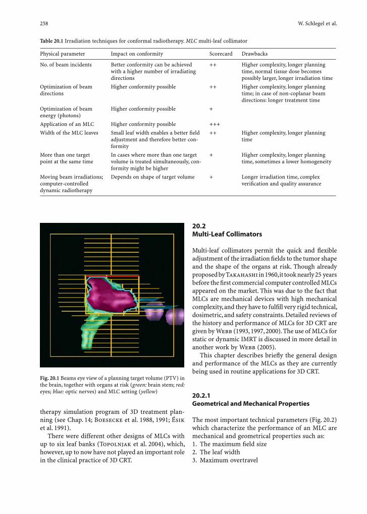
258 W. Schlegel et al.

therapy simulation program of 3D treatment plan-ning (see Chap. 14; Boesecke et al. 1988, 1991; Ésik et al. 1991).

There were different other designs of MLCs with up to six leaf banks (Topolnjak et al. 2004), which, however, up to now have not played an important role in the clinical practice of 3D CRT.

20.2 Multi-Leaf Collimators

Multi-leaf collimators permit the quick and fl exible adjustment of the irradiation fi elds to the tumor shape and the shape of the organs at risk. Though already proposed by Takahashi in 1960, it took nearly 25 years before the fi rst commercial computer controlled MLCs appeared on the market. This was due to the fact that MLCs are mechanical devices with high mechanical complexity, and they have to fulfi ll very rigid technical, dosimetric, and safety constraints. Detailed reviews of the history and performance of MLCs for 3D CRT are given by Webb (1993, 1997, 2000). The use of MLCs for static or dynamic IMRT is discussed in more detail in another work by Webb (2005).

This chapter describes briefl y the general design and performance of the MLCs as they are currently being used in routine applications for 3D CRT.

20.2.1 Geometrical and Mechanical Properties

The most important technical parameters (Fig. 20.2) which characterize the performance of an MLC are mechanical and geometrical properties such as:1. The maximum fi eld size2. The leaf width3. Maximum overtravel

Table 20.1 Irradiation techniques for conformal radiotherapy. MLC multi-leaf collimator

Physical parameter Impact on conformity Scorecard Drawbacks

No. of beam incidents Better conformity can be achieved with a higher number of irradiating directions

++ Higher complexity, longer planning time, normal tissue dose becomes possibly larger, longer irradiation time

Optimization of beam directions

Higher conformity possible ++ Higher complexity, longer planning time; in case of non-coplanar beam directions: longer treatment time

Optimization of beam energy (photons)

Higher conformity possible +

Application of an MLC Higher conformity possible +++

Width of the MLC leaves Small leaf width enables a better fi eld adjustment and therefore better con-formity

++ Higher complexity, longer planning time

More than one target point at the same time

In cases where more than one target volume is treated simultaneously, con-formity might be higher

+ Higher complexity, longer planning time, sometimes a lower homogeneity

Moving beam irradiations; computer-controlled dynamic radiotherapy

Depends on shape of target volume + Longer irradiation time, complex verifi cation and quality assurance

Fig. 20.1 Beams eye view of a planning target volume (PTV) in the brain, together with organs at risk (green: brain stem; red: eyes; blue: optic nerves) and MLC setting (yellow)

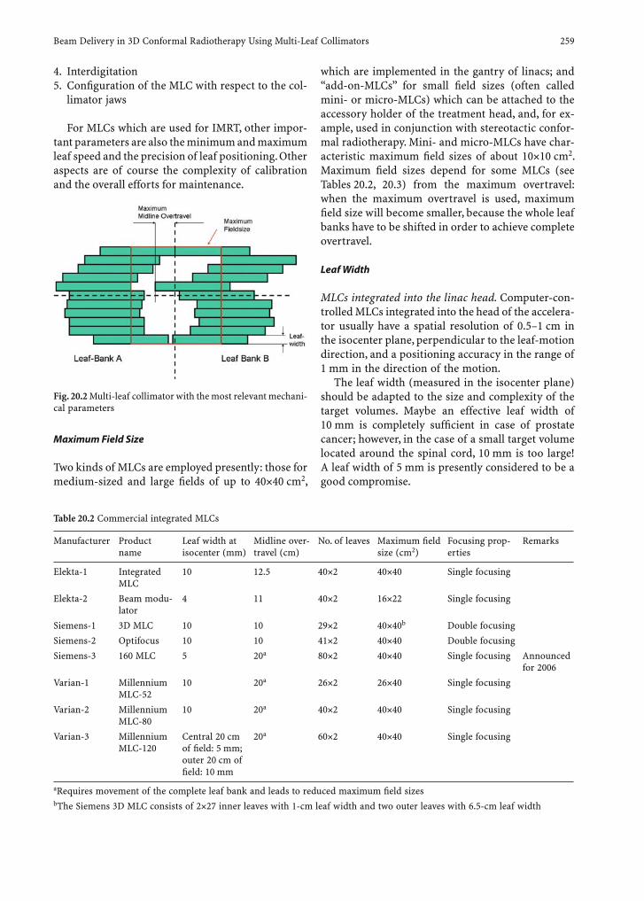
Beam Delivery in 3D Conformal Radiotherapy Using Multi-Leaf Collimators 259

4. Interdigitation5. Confi guration of the MLC with respect to the col-

limator jaws

For MLCs which are used for IMRT, other impor-tant parameters are also the minimum and maximum leaf speed and the precision of leaf positioning. Other aspects are of course the complexity of calibration and the overall efforts for maintenance.

which are implemented in the gantry of linacs; and “add-on-MLCs” for small fi eld sizes (often called mini- or micro-MLCs) which can be attached to the accessory holder of the treatment head, and, for ex-ample, used in conjunction with stereotactic confor-mal radiotherapy. Mini- and micro-MLCs have char-acteristic maximum fi eld sizes of about 10×10 cm2. Maximum fi eld sizes depend for some MLCs (see Tables 20.2, 20.3) from the maximum overtravel: when the maximum overtravel is used, maximum fi eld size will become smaller, because the whole leaf banks have to be shifted in order to achieve complete overtravel.

Leaf Width

MLCs integrated into the linac head. Computer-con-trolled MLCs integrated into the head of the accelera-tor usually have a spatial resolution of 0.5–1 cm in the isocenter plane, perpendicular to the leaf-motion direction, and a positioning accuracy in the range of 1 mm in the direction of the motion.

The leaf width (measured in the isocenter plane) should be adapted to the size and complexity of the target volumes. Maybe an effective leaf width of 10 mm is completely suffi cient in case of prostate cancer; however, in the case of a small target volume located around the spinal cord, 10 mm is too large! A leaf width of 5 mm is presently considered to be a good compromise.

Table 20.2 Commercial integrated MLCs

Manufacturer Product name

Leaf width at isocenter (mm)

Midline over-travel (cm)

No. of leaves Maximum fi eld size (cm2)

Focusing prop-erties

Remarks

Elekta-1 Integrated MLC

10 12.5 40×2 40×40 Single focusing

Elekta-2 Beam modu-lator

4 11 40×2 16×22 Single focusing

Siemens-1 3D MLC 10 10 29×2 40×40b Double focusing

Siemens-2 Optifocus 10 10 41×2 40×40 Double focusing

Siemens-3 160 MLC 5 20a 80×2 40×40 Single focusing Announced for 2006

Varian-1 Millennium MLC-52

10 20a 26×2 26×40 Single focusing

Varian-2 Millennium MLC-80

10 20a 40×2 40×40 Single focusing

Varian-3 Millennium MLC-120

Central 20 cm of fi eld: 5 mm; outer 20 cm of fi eld: 10 mm

20a 60×2 40×40 Single focusing

aRequires movement of the complete leaf bank and leads to reduced maximum fi eld sizesbThe Siemens 3D MLC consists of 2×27 inner leaves with 1-cm leaf width and two outer leaves with 6.5-cm leaf width

Fig. 20.2 Multi-leaf collimator with the most relevant mechani-cal parameters

Maximum Field Size

Two kinds of MLCs are employed presently: those for medium-sized and large fi elds of up to 40×40 cm2,

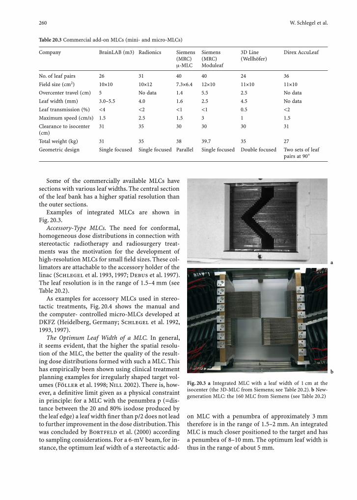
260 W. Schlegel et al.

Some of the commercially available MLCs have sections with various leaf widths. The central section of the leaf bank has a higher spatial resolution than the outer sections.

Examples of integrated MLCs are shown in Fig. 20.3.

Accessory-Type MLCs. The need for conformal, homogeneous dose distributions in connection with stereotactic radiotherapy and radiosurgery treat-ments was the motivation for the development of high-resolution MLCs for small fi eld sizes. These col-limators are attachable to the accessory holder of the linac (Schlegel et al. 1993, 1997; Debus et al. 1997). The leaf resolution is in the range of 1.5–4 mm (see Table 20.2).

As examples for accessory MLCs used in stereo-tactic treatments, Fig. 20.4 shows the manual and the computer- controlled micro-MLCs developed at DKFZ (Heidelberg, Germany; Schlegel et al. 1992, 1993, 1997).

The Optimum Leaf Width of a MLC. In general, it seems evident, that the higher the spatial resolu-tion of the MLC, the better the quality of the result-ing dose distributions formed with such a MLC. This has empirically been shown using clinical treatment planning examples for irregularly shaped target vol-umes (Föller et al. 1998; Nill 2002). There is, how-ever, a defi nitive limit given as a physical constraint in principle: for a MLC with the penumbra p (=dis-tance between the 20 and 80% isodose produced by the leaf edge) a leaf width fi ner than p/2 does not lead to further improvement in the dose distribution. This was concluded by Bortfeld et al. (2000) according to sampling considerations. For a 6-mV beam, for in-stance, the optimum leaf width of a stereotactic add-

Table 20.3 Commercial add-on MLCs (mini- and micro-MLCs)

Company BrainLAB (m3) Radionics Siemens (MRC)

-MLC

Siemens (MRC) Moduleaf

3D Line (Wellhöfer)

Direx AccuLeaf

No. of leaf pairs 26 31 40 40 24 36

Field size (cm2) 10×10 10×12 7.3×6.4 12×10 11×10 11×10

Overcenter travel (cm) 5 No data 1.4 5.5 2.5 No data

Leaf width (mm) 3.0–5.5 4.0 1.6 2.5 4.5 No data

Leaf transmission (%) <4 <2 <1 <1 0.5 <2

Maximum speed (cm/s) 1.5 2.5 1.5 3 1 1.5

Clearance to isocenter (cm)

31 35 30 30 30 31

Total weight (kg) 31 35 38 39.7 35 27

Geometric design Single focused Single focused Parallel Single focused Double focused Two sets of leaf pairs at 90°

Fig. 20.3 a Integrated MLC with a leaf width of 1 cm at the isocenter (the 3D-MLC from Siemens; see Table 20.2). b New-generation MLC: the 160 MLC from Siemens (see Table 20.2)

b

a

on MLC with a penumbra of approximately 3 mm therefore is in the range of 1.5–2 mm. An integrated MLC is much closer positioned to the target and has a penumbra of 8–10 mm. The optimum leaf width is thus in the range of about 5 mm.

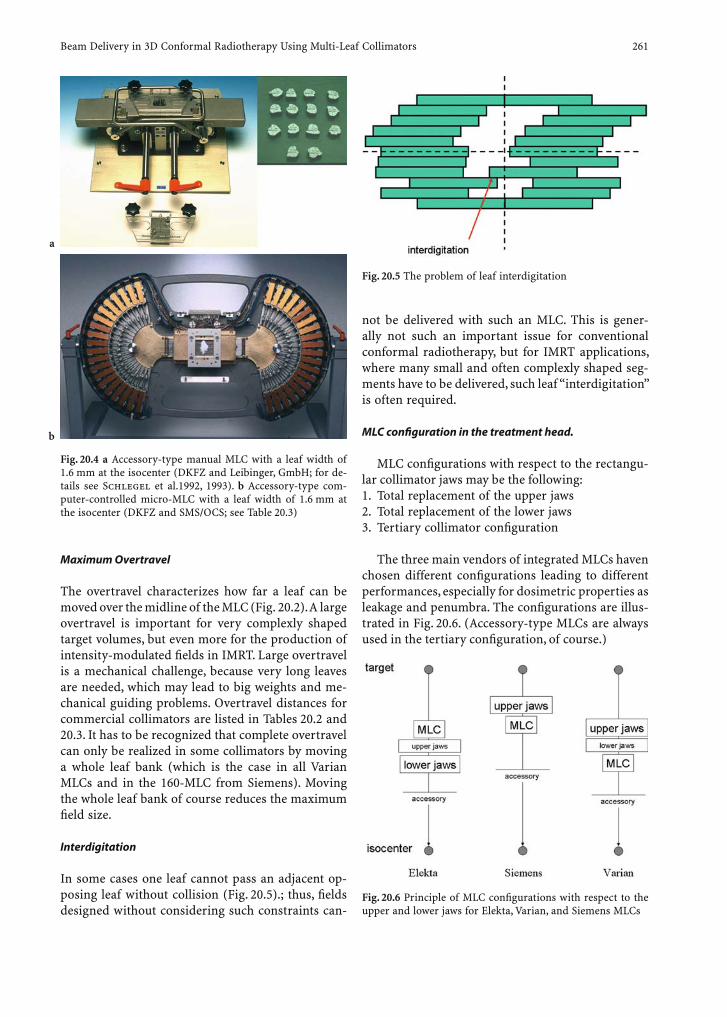
Beam Delivery in 3D Conformal Radiotherapy Using Multi-Leaf Collimators 261

Maximum Overtravel

The overtravel characterizes how far a leaf can be moved over the midline of the MLC (Fig. 20.2). A large overtravel is important for very complexly shaped target volumes, but even more for the production of intensity-modulated fi elds in IMRT. Large overtravel is a mechanical challenge, because very long leaves are needed, which may lead to big weights and me-chanical guiding problems. Overtravel distances for commercial collimators are listed in Tables 20.2 and 20.3. It has to be recognized that complete overtravel can only be realized in some collimators by moving a whole leaf bank (which is the case in all Varian MLCs and in the 160-MLC from Siemens). Moving the whole leaf bank of course reduces the maximum fi eld size.

Interdigitation

In some cases one leaf cannot pass an adjacent op-posing leaf without collision (Fig. 20.5).; thus, fi elds designed without considering such constraints can-

not be delivered with such an MLC. This is gener-ally not such an important issue for conventional conformal radiotherapy, but for IMRT applications, where many small and often complexly shaped seg-ments have to be delivered, such leaf “interdigitation” is often required.

MLC confi guration in the treatment head.

MLC confi gurations with respect to the rectangu-lar collimator jaws may be the following:1. Total replacement of the upper jaws2. Total replacement of the lower jaws3. Tertiary collimator confi guration

The three main vendors of integrated MLCs haven chosen different confi gurations leading to different performances, especially for dosimetric properties as leakage and penumbra. The confi gurations are illus-trated in Fig. 20.6. (Accessory-type MLCs are always used in the tertiary confi guration, of course.)

Fig. 20.4 a Accessory-type manual MLC with a leaf width of 1.6 mm at the isocenter (DKFZ and Leibinger, GmbH; for de-tails see Schlegel et al.1992, 1993). b Accessory-type com-puter-controlled micro-MLC with a leaf width of 1.6 mm at the isocenter (DKFZ and SMS/OCS; see Table 20.3)

Fig. 20.5 The problem of leaf interdigitation

b

a

Fig. 20.6 Principle of MLC confi gurations with respect to the upper and lower jaws for Elekta, Varian, and Siemens MLCs

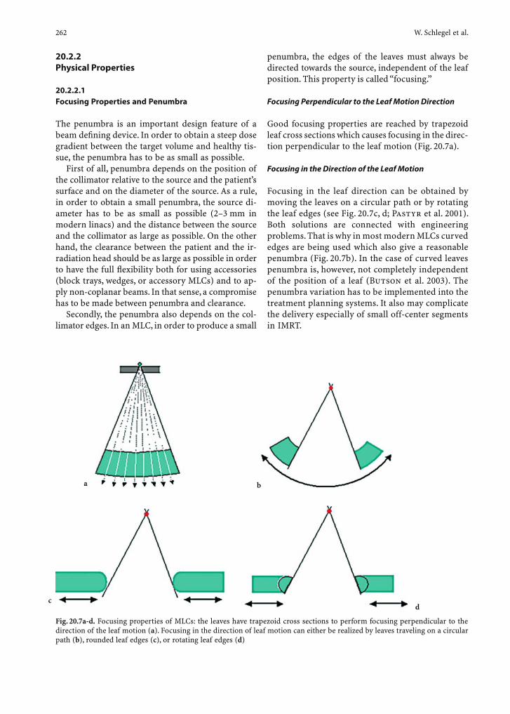
262 W. Schlegel et al.

20.2.2 Physical Properties

20.2.2.1 Focusing Properties and Penumbra

The penumbra is an important design feature of a beam defi ning device. In order to obtain a steep dose gradient between the target volume and healthy tis-sue, the penumbra has to be as small as possible.

First of all, penumbra depends on the position of the collimator relative to the source and the patient’s surface and on the diameter of the source. As a rule, in order to obtain a small penumbra, the source di-ameter has to be as small as possible (2–3 mm in modern linacs) and the distance between the source and the collimator as large as possible. On the other hand, the clearance between the patient and the ir-radiation head should be as large as possible in order to have the full fl exibility both for using accessories (block trays, wedges, or accessory MLCs) and to ap-ply non-coplanar beams. In that sense, a compromise has to be made between penumbra and clearance.

Secondly, the penumbra also depends on the col-limator edges. In an MLC, in order to produce a small

penumbra, the edges of the leaves must always be directed towards the source, independent of the leaf position. This property is called “focusing.”

Focusing Perpendicular to the Leaf Motion Direction

Good focusing properties are reached by trapezoid leaf cross sections which causes focusing in the direc-tion perpendicular to the leaf motion (Fig. 20.7a).

Focusing in the Direction of the Leaf Motion

Focusing in the leaf direction can be obtained by moving the leaves on a circular path or by rotating the leaf edges (see Fig. 20.7c, d; Pastyr et al. 2001). Both solutions are connected with engineering problems. That is why in most modern MLCs curved edges are being used which also give a reasonable penumbra (Fig. 20.7b). In the case of curved leaves penumbra is, however, not completely independent of the position of a leaf (Butson et al. 2003). The penumbra variation has to be implemented into the treatment planning systems. It also may complicate the delivery especially of small off-center segments in IMRT.

Fig. 20.7a-d. Focusing properties of MLCs: the leaves have trapezoid cross sections to perform focusing perpendicular to the direction of the leaf motion (a). Focusing in the direction of leaf motion can either be realized by leaves traveling on a circular path (b), rounded leaf edges (c), or rotating leaf edges (d)

ba

cd

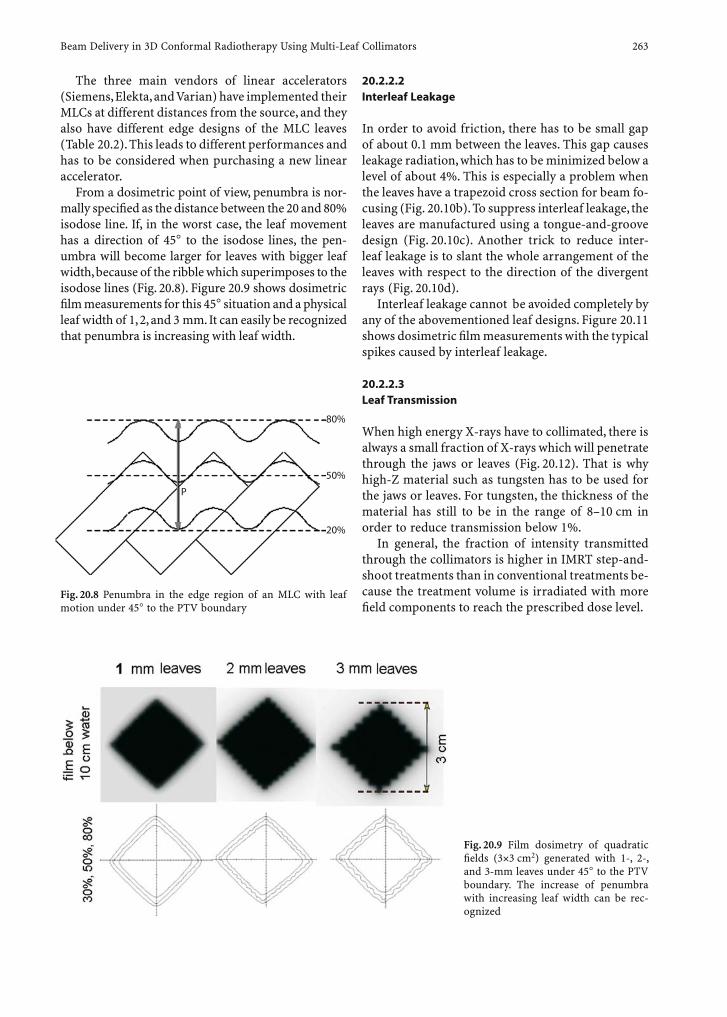
Beam Delivery in 3D Conformal Radiotherapy Using Multi-Leaf Collimators 263

The three main vendors of linear accelerators (Siemens, Elekta, and Varian) have implemented their MLCs at different distances from the source, and they also have different edge designs of the MLC leaves (Table 20.2). This leads to different performances and has to be considered when purchasing a new linear accelerator.

From a dosimetric point of view, penumbra is nor-mally specifi ed as the distance between the 20 and 80% isodose line. If, in the worst case, the leaf movement has a direction of 45° to the isodose lines, the pen-umbra will become larger for leaves with bigger leaf width, because of the ribble which superimposes to the isodose lines (Fig. 20.8). Figure 20.9 shows dosimetric fi lm measurements for this 45° situation and a physical leaf width of 1, 2, and 3 mm. It can easily be recognized that penumbra is increasing with leaf width.

20.2.2.2 Interleaf Leakage

In order to avoid friction, there has to be small gap of about 0.1 mm between the leaves. This gap causes leakage radiation, which has to be minimized below a level of about 4%. This is especially a problem when the leaves have a trapezoid cross section for beam fo-cusing (Fig. 20.10b). To suppress interleaf leakage, the leaves are manufactured using a tongue-and-groove design (Fig. 20.10c). Another trick to reduce inter-leaf leakage is to slant the whole arrangement of the leaves with respect to the direction of the divergent rays (Fig. 20.10d).

Interleaf leakage cannot be avoided completely by any of the abovementioned leaf designs. Figure 20.11 shows dosimetric fi lm measurements with the typical spikes caused by interleaf leakage.

20.2.2.3 Leaf Transmission

When high energy X-rays have to collimated, there is always a small fraction of X-rays which will penetrate through the jaws or leaves (Fig. 20.12). That is why high-Z material such as tungsten has to be used for the jaws or leaves. For tungsten, the thickness of the material has still to be in the range of 8–10 cm in order to reduce transmission below 1%.

In general, the fraction of intensity transmitted through the collimators is higher in IMRT step-and-shoot treatments than in conventional treatments be-cause the treatment volume is irradiated with more fi eld components to reach the prescribed dose level.

Fig. 20.9 Film dosimetry of quadratic fi elds (3×3 cm2) generated with 1-, 2-, and 3-mm leaves under 45° to the PTV boundary. The increase of penumbra with increasing leaf width can be rec-ognized

Fig. 20.8 Penumbra in the edge region of an MLC with leaf motion under 45° to the PTV boundary

80%

50%

20%

P

264 W. Schlegel et al.

At a rough guess, the transmitted intensity is twice the original physical level. If the transmission is, for example, 2%, the maximum of the transmit-ted intensity mounts up to 4% at some positions. Especially for MLCs used in IMRT, transmission as well as interleaf leakage should therefore be kept as low as possible.

Restrictions for leakage radiation of MLCs are given in IEC (1998): If the MLC is covered by rectan-gular jaws, which are automatically adjusted to the MLC shape, leakage radiation must be below 5% of an open 10×10-cm2 fi eld; otherwise, maximum leak-age should be less than 2% and average leakage less than 0.5%.

Fig. 20.12 Dose profi le measured with dosimetric fi lm under a completely closed accessory-type MLC. Leaf transmission and interleaf leakage can be detected

Fig. 20.11 Leaf transmission for leaves with height X and trans-mission coeffi cient

Fig. 20.10a-d. Various MLC concepts to prevent leakage a unfocused without correction, b focused without correction, c with tongue and groove, and d with fl ipped collimator

I(0)

I(d)=I(0) e- x

x

e

ba

c d

f

Beam Delivery in 3D Conformal Radiotherapy Using Multi-Leaf Collimators 265

20.2.3 Operating Modes

There are in principle two different operating modes for MLCs for 3D CRT, depending on whether the leaves are moving when the beam is on (dynamic mode) or the beam is shut off (static mode).

Although modern MLCs in principle have dynamic properties, they are still commonly applied in static treatment techniques. The real potential of MLCs in 3D CRT will be demonstrated in the future, when, for example, dynamic arc treatment techniques with MLCs will be more widely accepted and implemented to perform dynamic fi eld shaping.

The two modes (static mode=step-and-shoot technique; dynamic mode=sliding-window tech-nique) currently play a bigger role in IMRT delivery (see Chap. 23). In IMRT dynamic delivery is in many cases more time effi cient than step and shoot, but the step-and-shoot technique is less complex and qual-ity assurance may be easier to perform. Chui et al. (2001) compared the delivery of IMRT by dynamic and static techniques.

20.3 Commercial MLCs

20.3.1 Linac-Integrated MLCs

The major manufacturers of commercial MLCs inte-grated into the irradiation head of a linear accelera-tor are the companies Elekta, Siemens, and Varian. Galvin (1999) provides a useful review with tables of MLC properties. Huq et al. (2002) compared the MLCs of all three manufacturers using precisely the same criteria and experimental methods. The result of this investigation was that there is no clear su-periority of one vendor compared with the others: the different designs and confi gurations of the MLCs are leading to a balance of advantages and disadvan-tages and there was no clear superiority of one MLC compared with the others. An updated list of MLC characteristics is given in Table 20.2.

20.3.2 Accessory-Type MLCs

There are a couple of companies manufacturing and distributing accessory MLCs, which are especially

suited to treat small target volumes in conjunction with stereotactic irradiation techniques. Bortfeld et al. (1999) have provided an overview on the charac-teristics and performances of these mini- and micro-MLCs. The specifi cations of these add-on collimators are summarized in Table 20.3. In summary, MLCs of this type are closer positioned to the patient’s surface and have smaller leaf widths. As a consequence, mini- and micro-MLCs have much smaller penumbras and produce dose distributions with higher conformity; however, they are restricted to the treatment of small target volumes.

20.4 The Limits of Conventional Conformal Radiation Therapy

Complex-shaped target volumes close to radio-sensi-tive organs remain a challenge for the radiotherapist. With MLCs and conventional irradiation techniques conformal and homogeneous dose distributions can-not be obtained in all cases. This is particularly true for concave-shaped target volumes. In Chaps. 17 and 23 (Inverse planning and IMRT) of this book it is shown that as the result of a superposition of several irradiation segments with homogeneous intensity, a concave-shaped dose distribution is produced. The MLCs to produce these IMRT fi eld segments have to fulfi ll very special criteria concerning leaf speed, accuracy, and reproducibility of leaf positioning, overtravel, transmission, and leakage. The specifi c requirements of MLCs in IMRT are discussed and analyzed in much more detail by Schlegel and Mahr (2000) and Webb (2005).

References

Adams EJ, Cosgrove VP, Shepherd SF, Warrington AP, Bedford JL, Mubata CD, Bidmead AM, Brada M (1999) Comparison of a multi-leaf collimator with conformal blocks for the delivery of stereotactically guided conformal radiotherapy. Radiother Oncol 51:205–209

Boesecke R, Doll J, Bauer B, Schlegel W, Pastyr O, Lorenz WJ (1988) Treatment planning for conformation therapy using a multi-leaf collimator. Strahlenther Onkol 164:151–154

Boesecke R, Becker G, Alandt K, Pastyr O, Doll J, Schlegel W, Lorenz WJ (1991) Modifi cation of three-dimensional treatment planning system for the use of multi-leaf col-limators in conformation radiotherapy. Radiother Oncol 21:261–268

Bortfeld T, Schlegel W, Höver KH (1999) Mini- and micro-mul-tileaf collimators. Med Phys 26:1094

266 W. Schlegel et al.

Bortfeld T, Oelfke U, Nill S (2000) What is the optimum leaf width of a multileaf collimator? Med Phys 27:2494–2502

Butson MJ, Yu PK, Cheung T (2003) Rounded end multi-leaf penumbral measurements with radiochromic fi lm. Phys Med Biol 48:N247–N252

Chui CS, Chan MF, Yorke E, Spirou S, Ling CC (2001) Delivery of intensity modulated radiation therapy with a conven-tional multileaf collimator: comparison of dynamic and segmental methods. Med Phys 28 2441–2449

Debus J, Engenhart-Cabillic R, Holz FG, Pastyr O, Rhein B, Bortfeld T (1997) Stereotactic precision radiotherapy in the treatment of intraocular malignancies with a micro-multileaf collimator. Front Radiat Ther Oncol 30:39–46

Ésik O, Buerkelbach J, Boesecke R, Schlegel W, Németh G, Lorenz WJ (1991) Three-dimensional photon radiother-apy planning for laryngeal and hypopharyngeal cancers. 2. Conformation treatment planning using a multileaf col-limator. Radiother Oncol 20:238–244

Foroudi F, Lapsley H, Manderson C, Yeghiaian-Alvandi R (2000) Cost-minimization analysis: radiation treatment with and without a multi-leaf collimator. Int J Radiat Oncol Biol Phys 47:1443–1448

Föller M, Bortfeld T, Hädinger U, Häring P, Schulze C, Seeber S, Richter J, Schlegel W (1998) Beam shaping with a computer controllled micro-multileaf-collimator. Radiother Oncol 48 (Suppl 1):S76

Galvin JM (1999) The multileaf collimator: a complete guide. Proc AAPM Annual Meeting

Hartmann GH, Föhlisch F (2002) Dosimetric characterization of a new miniature multileaf collimator. Phys Med Biol 47:N171–N177

Hartmann GH, Pastyr O, Echner G, Hädinger U, Seeber S, Juschka J, Richter J, Schlegel W (2002) A new design for a mid-sized multileaf collimator (MLC). Radiother Oncol 64:S214

Huq MS, Das IJ, Steinberg T, Galvin JM (2002) A dosimetric comparison of various multileaf collimators. Phys Med Biol 47 N159–N170

IEC (1998) IEC 601-2-1, 2nd ednNill S, Tücking T, Münter M, Oelfke U (2002) IMRT with MLCs

of different leaf widths: a comparison of achievable dose distributions. Radiother Oncol 64 (Suppl 1):107–108

Pastyr O, Echner G, Hartmann GH, Richter J, Schlegel W (2001) Dynamic edge focussing: a new MLC-design to deliver IMRT with a double focussing high precision multi-leaf collimator. Radiother Oncol 61:S24

Schlegel W, Pastyr O, Bortfeld T, Becker G, Schad L, Gademann G, Lorenz WJ (1992) Computer systems and mechanical tools for stereotactically guided conformation therapy with linear accelerators. Int J Radiat Oncol Biol Phys 24:781–787

Schlegel W, Pastyr O, Bortfeld T, Gademann G, Menke M, Maier Borst W (1993) Stereotactically guided fractionated radio-therapy: technical aspects. Radiother Oncol 29:197–204

Schlegel W, Pastyr O, Kubesch R, Stein J, Diemer T, Höver KH, Rhein B (1997) A computer controlled micro-multileaf-col-limator for stereotactic conformal radiotherapy. In: Leavitt DD (ed) Proc XIIth Int Conf on the Use of Computers in Radiation Therapy. Medical Physics Publishing, Madison, Wisconsin, pp 79–82

Takahashi S (1965) Conformation radiotherapy: rotation techniques as applied to radiography and radiotherapy of cancer. Acta Radiol (Suppl 242):1–142

Topolnjak R, van der Heide UA, Raaymakers BW, Kotte AN, Welleweerd J, Lagendijk JJ (2004) A six-bank multi-leaf system for high precision shaping of large fi elds. Phys Med Biol 49:2645–2656

Webb S (ed) (1993) The physics of three-dimensional radia-tion therapy: conformal radiotherapy, radiosurgery and treatment planning. IOP Publishing, Bristol, UK

Webb S (ed) (1997) The physics of conformal radiotherapy: advances in technology IOP Publishing, Bristol, UK

Webb S (ed) (2000) Intensity modulated radiation therapy. IOP Publishing, Bristol, UK

Webb S (ed) (2005) Intensity modulated radiation therapy. Developing physics and clinical implementation. IOP Pub-lishing, Bristol, UK.

Stereotactic Radiotherapy/Radiosurgery 267

21 Stereotactic Radiotherapy/Radiosurgery

Anca-Ligia Grosu, Peter Kneschaurek, and Wolfgang Schlegel

A.-L. Grosu MD; P. Kneschaurek, PhDDepartment of Radiation Oncology, Klinikum rechts der Isar, Technical University, Ismaningerstrasse 22, 81675 Munich, GermanyW. Schlegel, PhDDeutsches Krebsforschungszentrum, Im Neuenheimer Feld 280, 69121 Heidelberg, Germany

21.1 Introduction

Stereotactic radiotherapy dates back more than 50 years; however, this form of treatment has entered the domain of radiation oncology only in the past 10–15 years. Initially an exotic technique, stereotactic radiotherapy has become an established, widespread treatment approach, characterized by the delivery of the irradiation with a very high geometrical preci-sion. The method is especially used for benign and

malignant cranial tumors but has lately been adapted to the body.

Stereotactic coordinates are used in the method-ology of different irradiation techniques: implanta-tion of seeds; Bragg-Peak irradiation; irradiation with gamma knife (Co60) or with linear accelerator (LINAC or X-Knife). This chapter focuses on the de-scription of the technique of stereotactic tele-ther-apy (percutaneous stereotactic radiotherapy) with LINAC, also known as stereotactic convergent beam irradiation. This is the most widespread irradiation technique using stereotactic coordinates.

21.2 Defi nition

Stereotaxy (stereo + taxis – Greek, orientation in space) is a method which defi nes a point in the pa-tient’s body by using an external three-dimensional coordinate system which is rigidly attached to the patient. Stereotactic radiotherapy uses this technique to position a target reference point, defi ned in the tumor, in the isocenter of the radiation machine (LINAC, gamma knife, etc.) with a high accuracy. This results in a highly precise delivery of the radiation dose to an exactly defi ned target (tumor) volume. The aim is to encompass the target volume in the high-dose area and, by means of a steep dose gradient, to spare the surrounding normal tissue. This allows the defi nition of the planning target volume (PTV) without, or with only a very small (1–2 mm), safety margin around the gross tumor volume (GTV) or the clinical target volume (CTV). Stereotactic radiother-apy is performed in various treatment techniques, including gamma-knife units using 60 Co photons, heavy charged particles, or neutron beams units and modifi ed LINAC units.

Treatment can be administered in a single fraction (radiosurgery, RS) or as multiple fractions (stereotac-tic fractionated radiotherapy, SFR). Some authors use the term stereotactic radiotherapy for the fraction-

CONTENTS

21.1 Introduction 26721.2 Defi nition 26721.3 Historical Background 26821.4 Stereotactic Coordinates 26821.5 Method of Stereotactic Irradiation Treatment 26921.5.1 Stereotactic Frame 26921.5.2 Imaging for Stereotactic Irradiation Treatment 27021.5.3 Treatment Planning 27221.5.3.1 Defi nition of Target Volume and Organs at Risk 27221.5.3.2 Defi nition of the Stereotactic Target Point 27221.5.3.3 Planning of the Radiation Technique 27221.5.3.4 3D Dose Calculation 27321.5.3.5 Dose Specifi cation 27321.5.3.6 Visualization of the Dose Distribution 27321.5.4 Positioning 27321.5.5 Delivery of the Radiation 27321.5.6 Quality Assurance 27421.6 Future Developments 27421.7 Conclusion 274 References 275

268 A.-L. Grosu et al.

ated delivery of the radiation; however, we consider it as a general term for all the irradiation treatments which are characterized by the integration of stereo-tactic coordinates in the treatment planning and de-livery, including the RS and the SFR.

The intention of RS is to produce enough cell kill within the target volume in a single fraction in order to eradicate the tumor. This single high irradiation dose can produce considerable side effects in normal tissue located close to the tumor or within the tar-get volume. The SFR combines the precision of target localization and dose application of RS with the ra-diobiological advantage of fractionated radiotherapy, i.e., breaking the total dose into smaller parts and thus allowing repair of DNA damage in normal tis-sue during the time between fractions. Time intervals of more than 6 h between fractions can signifi cantly reduce the risk of side effects in normal tissue (Hall and Brenner 1993; Schlegel et al. 1993).

21.3 Historical Background

The fi rst one to combine stereotactic methodology – which up to that point was used only in neurosurgery – with radiation therapy was the Swedish neurosur-geon Lars Leksell. He had the idea that X-ray could be used to treat certain neurological functional diseases instead of stereotactically guided needles used in neu-rosurgery. Leksel performed the fi rst treatment in 1951, at the Karolinska Institute, and called the new therapy approach radiosurgery (RS). The patient was fi xed in a stereotactic ring and irradiated with a precisely guided roentgen tube using 200-kV Röntgenbremsstrahlung (Leksell 1951). Bragg-peak studies with protons were begun in Uppsala, Boston, and Berkeley (Kjellberg et al. 1968; Larsson et al. 1958; Lawrence et al. 1962). In Berkeley Bragg-peak RS using helium ion beams was also developed (Lyman et al. 1977). Leksel con-tinued his work and built the fi rst isotope radiation machine, in 1968, the gamma knife.

The gamma-knife unit consists of 201 Co-60 sources arranged on the surface of a hemispherical shell, each aiming at an isocenter in a uniform dis-tance of 40 cm. Each source is collimated by a fi xed primary collimator and subsequently by a helmet, which consists of 201 collimators to which the patient and frame are attached and which is docked with the primary collimator array at the time of treatment. The helmets defi ne an approximately spherical dose distribution at the isocenter with nominal diameters

of 4, 8, 14, or 18 mm. The physical point of interest inside the patient is positioned at the isocenter of this distribution before treatment, and, if required, a sequence of treatment at different isocenters, with possibly different diameter helmets, are used to pro-duce a conformal dose distribution. Multiple isocen-ters treatments are required when the target shape is irregular. By combining several spherical dose distributions of smaller diameter in the appropriate location, it is possible to create a sum of isodose dis-tributions similar to the target volume. As a result the dose to the target itself is inhomogeneous, with larger number of isocenters leading to higher mean target doses. To date, the radiobiological consequences of dose inhomogeneity in tumor tissue cannot be eval-uated yet, but the advantages of dose escalation in the tumor and dose reduction in the normal tissue are undisputed (Lindquist et al. 1995; Verhey and Smith 1995).

The stereotactic radiation therapy with LINAC started in the early 1980s: the Swedish physicist Larsson proposed to use the LINAC instead Co 60 or protons (Larsson et al. 1974). The fi rst published reports on clinical use of LINAC came from Buenos Aires (Betti and Derechinsky 1983), Heidelberg (Hartmann et al. 1985), and Vicenza (Colombo et al. 1985), the authors of which all had developed the concept to deliver a single-dose radiation with con-vergent non-coplanar dynamic irradiation. Many clinical investigators made use of this technology all over the world in a very short time, showing, in comparison with the gamma-knife RS, comparable clinical results (Engenhart et al. 1989, 1992; Mehta et al. 1995; Becker et al. 1996; Debus et al. 1999). Further progress was made in LINAC stereotactic ra-diotherapy due to the development of non-invasive, replaceable head-fi xation systems, which allow the implementation of the dose fractionation (Schlegel et al. 1992, 1993; Stärk et al. 1997). Another impor-tant development is the micro-multileaf collimator which permits the adoption of the irradiated area to irregular-shaped target volumes (Schlegel et al. 1997) and the extension of the stereotactic irradia-tion technique to the head and neck (Gademann et al. 1993) and the body (Herfarth et al. 2000).

21.4 Stereotactic Coordinates

The key idea of all stereotactic radiation therapy techniques is the use of stereotactic coordinates to

Stereotactic Radiotherapy/Radiosurgery 269

defi ne the volume which has to be irradiated three dimensionally; therefore, target volume and anatomi-cal structures are localized in the space defi ned by the stereotactic coordinates system. Computed tomogra-phy (CT) or magnetic resonance imaging (MRI) are used for defi ning the anatomical structures which are of crucial importance for radiation therapy. The stereotactic localizer which is imaged simultaneously allows transfer of the image coordinates into the ste-reotactic coordinates system. During the planning of the radiation therapy a target point in the stereotactic space is defi ned. Before onset of radiation the patient is positioned in such a way that this target point is placed in the isocenter of the radiation machine with the help of the stereotactic positioning system.

In general, the stereotactic coordinates are a carte-sian three-dimensional coordinates system attached to the stereotactic frame in a rigid relationship. The origin of the stereotactic coordinates system is gen-erally in the center of the volume defi ned by the ste-reotactic frame: the x and y axes correspond to the lateral and frontal side of the frame and the z axis to the cranio-caudal direction (Fig. 21.1).

3. Treatment planning4. Positioning of the patient for the stereotactic radi-

ation therapy5. Delivery of the irradiation6. Quality assurance

21.5.1 Stereotactic Frame

Stereotactic radiotherapy is based on the rigid con-nection of the stereotactic frame to the patient during CT, MRI, and angiography imaging (Figs. 21.2, 21.3). The stereotactic frame is the base for the fi xation of the other stereotactic elements (localizer and posi-tioner) and for the defi nition of the origin (point 0) of

Fig. 21.1 The stereotactic coordinates defi ne three-dimension-ally the space which has to be irradiated

21.5 Method of Stereotactic Irradiation Treatment

The main steps in the planning and delivering of stereotactic irradiation treatment are:1. Rigid application of the stereotactic frame to the

patient2. Imaging (CT, MRI, angiography) of the patient

with the frame and localizer attached to the frame

Fig. 21.3 Non-invasive repeat head fi xation with the mask sys-tem and upper jaw support

Fig. 21.2 Head-ring fi xation. A Carbon fi ber posts. B, E Artifact-free fi xation pins with ceramic tips. C Robust and lightweight frame. D Two torque wrenches for pressure adjustment of pins

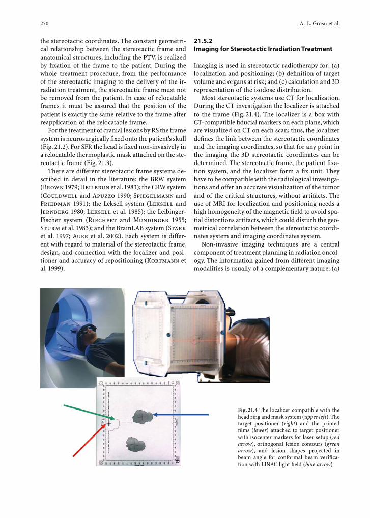
270 A.-L. Grosu et al.

the stereotactic coordinates. The constant geometri-cal relationship between the stereotactic frame and anatomical structures, including the PTV, is realized by fi xation of the frame to the patient. During the whole treatment procedure, from the performance of the stereotactic imaging to the delivery of the ir-radiation treatment, the stereotactic frame must not be removed from the patient. In case of relocatable frames it must be assured that the position of the patient is exactly the same relative to the frame after reapplication of the relocatable frame.

For the treatment of cranial lesions by RS the frame system is neurosurgically fi xed onto the patient’s skull (Fig. 21.2). For SFR the head is fi xed non-invasively in a relocatable thermoplastic mask attached on the ste-reotactic frame (Fig. 21.3).

There are different stereotactic frame systems de-scribed in detail in the literature: the BRW system (Brown 1979; Heilbrun et al. 1983); the CRW system (Couldwell and Apuzzo 1990; Spiegelmann and Friedman 1991); the Leksell system (Leksell and Jernberg 1980; Leksell et al. 1985); the Leibinger-Fischer system (Riechert and Mundinger 1955; Sturm et al. 1983); and the BrainLAB system (Stärk et al. 1997; Auer et al. 2002). Each system is differ-ent with regard to material of the stereotactic frame, design, and connection with the localizer and posi-tioner and accuracy of repositioning (Kortmann et al. 1999).

21.5.2 Imaging for Stereotactic Irradiation Treatment

Imaging is used in stereotactic radiotherapy for: (a) localization and positioning; (b) defi nition of target volume and organs at risk; and (c) calculation and 3D representation of the isodose distribution.

Most stereotactic systems use CT for localization. During the CT investigation the localizer is attached to the frame (Fig. 21.4). The localizer is a box with CT-compatible fi ducial markers on each plane, which are visualized on CT on each scan; thus, the localizer defi nes the link between the stereotactic coordinates and the imaging coordinates, so that for any point in the imaging the 3D stereotactic coordinates can be determined. The stereotactic frame, the patient fi xa-tion system, and the localizer form a fi x unit. They have to be compatible with the radiological investiga-tions and offer an accurate visualization of the tumor and of the critical structures, without artifacts. The use of MRI for localization and positioning needs a high homogeneity of the magnetic fi eld to avoid spa-tial distortions artifacts, which could disturb the geo-metrical correlation between the stereotactic coordi-nates system and imaging coordinates system.

Non-invasive imaging techniques are a central component of treatment planning in radiation oncol-ogy. The information gained from different imaging modalities is usually of a complementary nature: (a)

Fig. 21.4 The localizer compatible with the head ring and mask system (upper left). The target positioner (right) and the printed fi lms (lower) attached to target positioner with isocenter markers for laser setup (red arrow), orthogonal lesion contours (green arrow), and lesion shapes projected in beam angle for conformal beam verifi ca-tion with LINAC light fi eld (blue arrow)

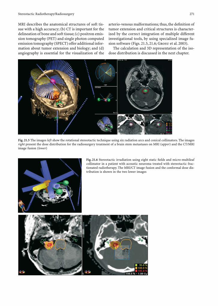
Stereotactic Radiotherapy/Radiosurgery 271

MRI describes the anatomical structures of soft tis-sue with a high accuracy; (b) CT is important for the delineation of bone and soft tissue; (c) positron emis-sion tomography (PET) and single photon computed emission tomography (SPECT) offer additional infor-mation about tumor extension and biology; and (d) angiography is essential for the visualization of the

arterio-venous malformations; thus, the defi nition of tumor extension and critical structures is character-ized by the correct integration of multiple different investigational tools, by using specialized image fu-sion software (Figs. 21.5, 21.6; Grosu et al. 2003).

The calculation and 3D representation of the iso-dose distribution is discussed in the next chapter.

Fig. 21.5 The images left show the rotational stereotactic technique using six radiation arcs and conical collimators. The images right present the dose distribution for the radiosurgery treatment of a brain stem metastases on MRI (upper) and the CT/MRI image fusion (lower)

Fig. 21.6 Stereotactic irradiation using eight static fi elds and micro-multileaf collimator in a patient with acoustic neuroma treated with stereotactic frac-tionated radiotherapy. The MRI/CT image fusion and the conformal dose dis-tribution is shown in the two lower images

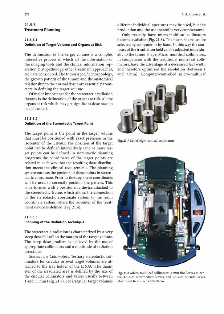
272 A.-L. Grosu et al.

21.5.3 Treatment Planning

21.5.3.1 Defi nition of Target Volume and Organs at Risk

The delineation of the target volume is a complex interactive process in which all the information of the imaging tools and the clinical information (op-eration, histopathology, other treatment approaches, etc.) are considered. The tumor-specifi c morphology, the growth pattern of the tumor, and the anatomical relationship to the normal tissue are essential param-eters in defi ning the target volume.

Of major importance for the stereotactic radiation therapy is the delineation of the organs at risk. All the organs at risk which may get signifi cant dose have to be delineated.

21.5.3.2 Defi nition of the Stereotactic Target Point

The target point is the point in the target volume that must be positioned with exact precision in the isocenter of the LINAC. The position of the target point can be defi ned interactively. One or more tar-get points can be defi ned. In stereotactic planning programs the coordinates of the target points are related in such way that the resulting dose distribu-tion meets the clinical requirements. The planning system outputs the position of these points in stereo-tactic coordinate. Prior to therapy, these coordinates will be used to correctly position the patient. This is performed with a positioner, a device attached to the stereotactic frame, which allows the connection of the stereotactic coordinate system to the room coordinate system, where the isocenter of the treat-ment device is defi ned (Fig. 21.4).

21.5.3.3 Planning of the Radiation Technique

The stereotactic radiation is characterized by a very steep dose fall-off on the margin of the target volume. The steep dose gradient is achieved by the use of appropriate collimators and a multitude of radiation directions.

Stereotactic Collimators. Tertiary stereotactic col-limators for circular or oval target volumes are at-tached to the tray holder of the LINAC. The diam-eter of the irradiated area is defi ned by the size of the circular collimators and varies usually between 1 and 35 mm (Fig. 21.7). For irregular target volumes

different individual apertures may be used, but the production and the use thereof is very cumbersome.

Only recently have micro-multileaf collimators become available (Fig. 21.8). The beam shape can be selected by computer or by hand. In this way the con-tours of the irradiation fi eld can be adjusted individu-ally to the tumor shape. Micro-multileaf collimators, in comparison with the traditional multi-leaf colli-mators, have the advantage of a decreased leaf width and therefore optimized the resolution (between 1 and 3 mm). Computer-controlled micro-multileaf

Fig. 21.8 Micro-multileaf collimator: 3-mm fi ne leaves at cen-ter; 4.5-mm intermediate leaves; and 5.5-mm outside leaves. Maximum fi eld size is 10×10 cm

Fig. 21.7 Set of eight conical collimators

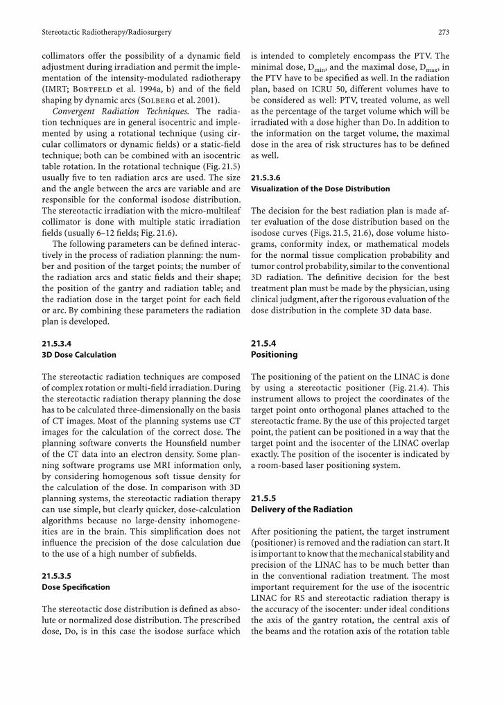
Stereotactic Radiotherapy/Radiosurgery 273

collimators offer the possibility of a dynamic fi eld adjustment during irradiation and permit the imple-mentation of the intensity-modulated radiotherapy (IMRT; Bortfeld et al. 1994a, b) and of the fi eld shaping by dynamic arcs (Solberg et al. 2001).

Convergent Radiation Techniques. The radia-tion techniques are in general isocentric and imple-mented by using a rotational technique (using cir-cular collimators or dynamic fi elds) or a static-fi eld technique; both can be combined with an isocentric table rotation. In the rotational technique (Fig. 21.5) usually fi ve to ten radiation arcs are used. The size and the angle between the arcs are variable and are responsible for the conformal isodose distribution. The stereotactic irradiation with the micro-multileaf collimator is done with multiple static irradiation fi elds (usually 6–12 fi elds; Fig. 21.6).

The following parameters can be defi ned interac-tively in the process of radiation planning: the num-ber and position of the target points; the number of the radiation arcs and static fi elds and their shape; the position of the gantry and radiation table; and the radiation dose in the target point for each fi eld or arc. By combining these parameters the radiation plan is developed.

21.5.3.4 3D Dose Calculation

The stereotactic radiation techniques are composed of complex rotation or multi-fi eld irradiation. During the stereotactic radiation therapy planning the dose has to be calculated three-dimensionally on the basis of CT images. Most of the planning systems use CT images for the calculation of the correct dose. The planning software converts the Hounsfi eld number of the CT data into an electron density. Some plan-ning software programs use MRI information only, by considering homogenous soft tissue density for the calculation of the dose. In comparison with 3D planning systems, the stereotactic radiation therapy can use simple, but clearly quicker, dose-calculation algorithms because no large-density inhomogene-ities are in the brain. This simplifi cation does not infl uence the precision of the dose calculation due to the use of a high number of subfi elds.

21.5.3.5 Dose Specifi cation

The stereotactic dose distribution is defi ned as abso-lute or normalized dose distribution. The prescribed dose, Do, is in this case the isodose surface which

is intended to completely encompass the PTV. The minimal dose, Dmin, and the maximal dose, Dmax, in the PTV have to be specifi ed as well. In the radiation plan, based on ICRU 50, different volumes have to be considered as well: PTV, treated volume, as well as the percentage of the target volume which will be irradiated with a dose higher than Do. In addition to the information on the target volume, the maximal dose in the area of risk structures has to be defi ned as well.

21.5.3.6 Visualization of the Dose Distribution

The decision for the best radiation plan is made af-ter evaluation of the dose distribution based on the isodose curves (Figs. 21.5, 21.6), dose volume histo-grams, conformity index, or mathematical models for the normal tissue complication probability and tumor control probability, similar to the conventional 3D radiation. The defi nitive decision for the best treatment plan must be made by the physician, using clinical judgment, after the rigorous evaluation of the dose distribution in the complete 3D data base.

21.5.4 Positioning

The positioning of the patient on the LINAC is done by using a stereotactic positioner (Fig. 21.4). This instrument allows to project the coordinates of the target point onto orthogonal planes attached to the stereotactic frame. By the use of this projected target point, the patient can be positioned in a way that the target point and the isocenter of the LINAC overlap exactly. The position of the isocenter is indicated by a room-based laser positioning system.

21.5.5 Delivery of the Radiation

After positioning the patient, the target instrument (positioner) is removed and the radiation can start. It is important to know that the mechanical stability and precision of the LINAC has to be much better than in the conventional radiation treatment. The most important requirement for the use of the isocentric LINAC for RS and stereotactic radiation therapy is the accuracy of the isocenter: under ideal conditions the axis of the gantry rotation, the central axis of the beams and the rotation axis of the rotation table

274 A.-L. Grosu et al.

convert in one point, the isocenter. In practical terms these requirements cannot be achieved. In general, it is acceptable that the three axes – gantry rotation axis, central axis, and table rotation axis – meet in a sphere which coincides with the isocenter and has a diameter of approximately 1 mm. The amount of inaccuracy in the LINAC isocenter is similar to the imprecision of target volume and target point defi ni-tion with modern radiological techniques. Despite the high weight of the LINAC and of the patient ta-ble, these mechanical requirements can be achieved. They must be constantly controlled during regular quality-control procedures.

21.5.6 Quality Assurance

The essential requirement for the clinical use of the LINAC is quality control based on well-defi ned pro-tocols (Report of Task Group 42, 1995, DIN 6827-1, 2001). These quality requirements are different from those needed in conventional radiotherapy (ICRU Report 50, 1984). The quality-assurance protocols address the precision of the target volume and target point with CT, MRI, PET and angiography, the dosim-etry, the planning of the irradiation, and especially with the calibration of the absolute dose and of the dose application. For the quality-assurance assess-ment proper phantoms and specialized dosimetric instruments must be available. Excellent documenta-tion of quality-control requirements have been pub-lished by Hartman (1995).

21.6 Future Developments

The stereotactic radiation therapy originated from RS and has been further developed into a fraction-ated stereotactic radiation therapy. The use of this method at present is still limited predominantly to central nervous system lesions. The use of stereotac-tic radiation therapy for other regions of the body (paravertebral tumors as well as in tumors of the liver, lung, and pelvis) is under development. The fi rst clinical results are promising (Herfarth et al. 2000; Zimmermann et al. 2004).

The combination of the stereotactic radiation therapy of the LINAC with IMRT opens new perspec-tives for those entities where exact conformal and high doses must be delivered (Khoo et al. 1999).

The fi rst analysis of RS with dynamic fi eld shap-ing technique in comparison with conformal static beams and multi-isocentric non-coplanar circular arcs showed that the dynamic-arc technique com-bines simple planning, short treatment times, dose homogeneity within the target, and rapid dose fall-off in normal tissue (Solberg et al. 2001; Stärk et al. 2004).

A new method under development is robot-as-sisted RS. The LINAC in this device is mounted on a robotic arm with 6 degrees of freedom. This Cyber-Knife at this time point can only be used for static radiation, but principally it can be developed for dy-namic fi elds as well (Yu et al. 2004; Gerszten et al. 2004).

In past years progress has been made in the fi eld of frameless stereotactic radiation therapy. This method aims at delivering stereotactic radiation therapy without the stereotactic frame and thus does not use an invasive fi xation system, but is still re-quired to deliver the radiation dose with a precision of 1 mm. Frameless stereotactic therapy originated in neurosurgery. For neuronavigation internal and ex-ternal markers are used for positioning the patient with stereoscopic video cameras and X-ray machines. Despite the high potential of frameless stereotactic treatments, the stereotactic frame will remain the standard. In stereotactic radiation therapy the frame is not only used for target localization but also for the exact positioning of the patient on the LINAC and for patient immobilization during the treatment.

21.7 Conclusion

Both RS and SFS have gained eminent positions in radiation oncology and have become established modalities in the treatment of cranial lesions. Most leading radiation departments offer this technique and their numbers have grown signifi cantly in the past decade.

The LINAC RS and gamma knife RS are equiva-lent techniques; however, technological and physical differences between these two methods have led to some confusion. Considering the RS, comparative clinical studies have documented that both therapeu-tic methodologies can be used with similar results. In comparison with gamma knife, the use of LINAC technology offers the possibility of dose fraction-ation, which has substantial clinical implications. The quality control of the complex LINAC is higher than

Stereotactic Radiotherapy/Radiosurgery 275

of gamma knife and requires a specialized team of medical physicists and radiation oncologists. On the other hand, it is undisputed that stereotactic radiation therapy with isocentric LINAC has a high potential for further developments. Examples in this direction are the introduction of computer-guided micro-mul-tileaf collimators which allows the delivery of a con-form dose distribution with only one isocenter, using static fi elds or dynamic arcs and the implementation of the stereotactic intensity-modulated radiotherapy. These new technologies amplify substantially the po-tential of the stereotactic modality.

References

Auer F, Grosu AL, Wiedenmann N et al. (2002) Stereotactic radiotherapy in patients with brain tumors: accuracy of a modifi ed mask system. In: Kogelnik HD, Lukas P, Sedl-mayer E (eds) Progress in radio-oncology, vol 7. Monduzzi Editore International Proc Division, Bologna, pp 163–168

Becker G, Kortmann R, Kaulich TW et al. (1996) Gamma-Knife versus stereotaktische Linearbeschleunigerbestrahlung. Radiologe 36:345–353

Betti O, Derechinsky VE (1983) Irradiation stereotaxique mul-tifasceaux. Neurochirurgie 29:295–298

Bortfeld TR, Boyer AL, Schlegel W et al. (1994a) Realization and verifi cation of three-dimensional conformal radio-therapy with modulated fi elds. Int J Radiat Oncol Biol Phys 30:899–908

Bortfeld TR, Kahler DL, Waldron TJ et al. (1994b) X-ray fi eld compensation with multileaf collimators. Int J Radiat Oncol Biol Phys 28:723–730

Brown RA (1979) Stereotactic headframe for use with CT body scanners. Invest Radiol 14:300–304

Couldwell WT, Apuzzo MLJ (1990) Initial experience related to the use of the Cosman-Roberts-Wells stereotactic instru-ment. J Neurosurg 72:145–148

Colombo F, Benedetti A, Pozza F et al. (1985) External ste-reotactic irradiation by linear accelerator. Neurosurgery 16:154–160

Debus J, Pirzkall A, Schlegel W et al. (1999) Stereotaktische Einzeitbestrahlung (Radiochirurgie). Strahlenther Onkol 175:47–56

DIN 6827-1, Protokollierung bei der medizinischen Anwen-dung ionisierender Strahlung. Teil 1: Therapie mit Elek-tronenbeschleuniger sowie Röntgen- und Gammabestrah-lungseinrichtungen, Deutsches Institut für Industrie-Nor-mung, 2001

Engenhart R, Kimmig B, Sturm V (1989) Stereotactically guided convergent beam irradiation of solitary brain metastasis and cerebral arteriovenous malformations: In: Dyck P, Bouzaglou A (eds) Brachytherapy of brain tumors and related stereotactic treatment. Hanley and Belfus, Phil-adelphia, pp 119–132

Engenhart R, Wowra B, Kimmig B et al. (1992) Stereotakti-sche Konvergenzbestrahlung: Aktuelle Perspektiven auf der Grundlage klinischer Ergebnisse. Strahlenther Onkol 168:245–259

Gademann G, Schlegel W, Debus J et al. (1993) Fractionated stereotactically guided radiotherapy of head and neck tumors: a report on clinical use of a new system in 195 cases. Radiother Oncol 29:205–213

Gerszten PC, Ozhasoglu C, Burton SA et al. (2004) CyberKnife frameless stereotactic radiosurgery for spinal lesion: clini-cal experience in 125 cases. Neurosurgery 55:89–98

Grosu AL, Lachner R, Wiedenmann N, Stärk S, Thamm R, Kneschaurek P, Schwaiger M, Molls M, Weber WA (2003) Validation of a method for automatic fusion of CT- and C11-Methionine-PET datasets of the brain for stereotactic radiotherapy using a LINAC. First clinical experience. Int J Radiat Oncol Biol Phys 56:1450–1463

Hall EJ, Brenner DJ (1993) The radiobiology of RS: rationale for different treatment regimes for AVMs and malignan-cies. Int J Radiat Oncol Biol Phys 25:381–385

Hartmann GH (ed) (1995) Quality assurance program on ste-reotactic radiosurgery. Springer, Berlin Heidelberg New York

Hartmann GH, Schlegel W, Sturm V et al. (1985) Cerebral radiation surgery using moving fi eld irradiation at a linac facility. Int J Radiat Oncol Biol Phys 11:185–192

Heilbrun M, Roberts T, Apuzzo M et al. (1983) Preliminary experience with Brown-Roberts-Wells (BRW) computer-ized tomography stereotaxic guidance system. J Neurosurg 59:217–222

Herfarth KK, Debus J, Lohr F et al. (2000) Extracranial ste-reotactic radiation therapy: set-up accuracy of patients treated for liver metastases. Int J Radiat Oncol Biol Phys 46:329–335

ICRU Report 50 (1984) Prescribing, recording and reporting photon beam therapy. ICRU, Washington, DC

Khoo V, Oldham M, Adams E et al. (1999) Comparison of intensity-modulated tomotherapy with stereotactically guided conformal radiotherapy for brain tumors. Int J Radiat Oncol Biol Phys 45:415–425

Kjellberg RN, Shintani A, Frantz AG (1968) Proton beams in acromegaly. N Engl J Med 278:689–695

Kortmann RD, Becker G, Perelmouter J et al. (1999) Geomet-ric accuracy of fi eld alignment in fractionated stereotactic conformal radiotherapy of brain tumors. Int J Radiat Oncol Biol Phys 43:921–926

Larsson B, Leksell L, Rexed B et al. (1958) The high energy proton beam as a neurosurgical tool. Nature 182:1222–1223

Larsson B, Liden K, Sorby B (1974) Irradiation of small struc-tures through intact skull. Acta Radiol Ther Phys Biol 13:513–534

Lawrence JH, Tobias CA, Bom JL et al. (1962) Heavy particle irradiation in neo-plasic and neurosurgical disease. J Neu-rosurg 19:717–722

Leksell L (1951) The stereotactic method and radiosurgery of the brain. Acta Chir Scand 102:316–319

Leksell L, Jernberg B (1980) Stereotaxis and tomography. A technical note. Acta Neurochir 52:1–7

Leksell L, Leksell D, Schwebel Y (1985) Stereotaxis and nuclear magnetic resonance. J Neurol Neurosurg Psychiatry 48:14–18

Lindquist C (1995) Gamma Knife radiosurgery. Semin Radiat Oncol 5:197–202

Lyman JT, Howard J (1977) Dosimetry and instrumentation for helium and heavy ions. Int J Radiat Oncol Biol Phys 3:81–85

276 A.-L. Grosu et al.

Mehta M, Noyes WR, Mackie TR (1995) Linear accelera-tor confi gurations for radiosurgery. Semin Radiat Oncol 5:203–212

Report of Task Group 42 (1995) Radiation Therapy Committee, AAPM Report no. 54, Schell MC (Chairman), Bova FJ, Larson DA et al., published for the American Association of Physi-cists in Medicine by the American Institute of Physics

Riechert T, Mundinger F (1955) Beschreibung und Anwendung eines Zielgerätes für stereotaktische Hirnoperationen. Acta Neurochir 3 (Suppl):308–337

Schlegel W, Pastyr O, Bortfeld T et al. (1992) Computer systems and mechanical tools for stereotactically guided conforma-tion therapy with linear accelerators. Int J Radiat Oncol Biol Phys 24:781–787

Schlegel W, Pastyr O, Bortfeld T et al. (1993) Stereotactically guided fractionated radiotherapy: technical aspects. Radi-other Oncol 29:197–204

Schlegel W, Pastyr O, Kubesch R et al. (1997) A computer con-trolled micro-multileaf-collimator for stereotactic confor-mal radiotherapy. In: In: Leavitt DD (ed) Proc XIIth Inter-national Conference on the Use of Computers in Radio-therapy (ICCR). Medical Physics Publishing, Madison, Wisconsin, pp 163–165

Solberg TD, Boedeker KL, DeSalles AAF (2001) Dynamic arc

radiosurgery fi eld shaping: a comparison with static fi eld conformal and noncoplanar circular arcs. Int J Radiat Oncol Biol Phys 49:1482–1491

Spiegelmann R, Friedman WA (1991) Stereotactic suboccipi-tal transcerebellar biopsy under local anesthesia using the Cosman-Roberts-Wells frame. J Neurosurg 75:486–488

Stärk S, Grosu AL, Molls M et al. (1997) Maskentechnik der Firma BrainLAB – Nicht – invasive Fixierung bei stereotak-tischen Strahlentherapie von Läsionen im Gehirn. Biomed Tech 42:352–353

Stärk S, Grosu AL, Kneschaurek P (2004) Dynamic arc stereo-tactic radiotherapy. J Radiat Oncol Biol Phys

Sturm V, Pastyr O, Schlegel W (1983) Stereotactic computer tomography with a modifi ed Riechert-Mundinger device as the basis for integrated stereotactic neuroradiological investigations. Acta Neurochir 68:11–17

Verhey LJ, Smith V (1995) The physics of radiosurgery. Semin Radiat Oncol 5:175–191

Yu C, Main W, Taylor D, Kuduvalli G et al. (2004) An anthro-pomorphic phantom study of the accuracy of CyberKnife spinal radiosurgery. Neurosurgery 55:1138–1149

Zimmermann FB, Geinitz H, Schill S, Grosu AL et al. (2005) Ste-reotactic fractionated radiation therapy for stage I non small cell lung cancer. Initial results. Lung Cancer 48:107–114

Extracranial Stereotactic Radiation Therapy 277

22 Extracranial Stereotactic Radiation Therapy

Klaus K. Herfarth

K.K. Herfarth, MDDepartment of Radiation Oncology, University of Heidelberg, Im Neuenheimer Feld 400, 69120 Heidelberg, Germany

22.1 History

The use of a 3D stereotactic system for radiation therapy was fi rst described by Leksell with the de-velopment of the gamma knife (LEKSELL 1951). The head was invasively attached to a stereotactic frame. Numerous cobalt sources could be individually fo-cused to the isocenter allowing a precise application of a focused high dose with a deep dose gradient to the surrounding tissues. With the development of lin-ear accelerators, the stereotactic system was adapted with the serial application of collimated beams to the specifi ed isocenter (HARTMANN et al. 1985). Again, only targets in the head could be treated when the head was fi xed with a stereotactic ring. Several approaches using non-invasive fi xation methods in a stereotactic environment made a fractionated stereotactic radia-tion treatment in the head possible. New systems of immobilization have had to be developed for stereo-tactic treatments of extracranial targets. Two major uncertainties have to be taken into account: a reliable fi xation of the body is more diffi cult to achieve than

of the head. On the other hand, organ motion has a major impact on the accuracy of the stereotactic system in some of the extracranial targets.

The Karolinska group around Blomgren and Lax published the fi rst extracranial stereotactic system, the stereotactic body frame (SFB), in 1994 (LAX et al. 1994). One year later, HAMILTON and LULU (1995), from the University of Tucson, Arizona, presented a different prototype of extracranial stereotactic sys-tem, which was originally developed at the German Cancer Research Center .

Several systems for extracranial stereotactic treat-ment, the accuracy, advantages, and disadvantages are discussed in the following section. Published clinical data of stereotactic treatments of extracranial targets are summarized later in this chapter.

22.2 Systems and Setup

There are several systems available for stereotactic immobilization of the body stem. For some of these systems, data about the positioning accuracy has been published.

The stereotactic body frame (SFB, Elekta) con-sists construction of plastic and wood over a length of approximately 1 m. Indicators for calculation of the stereotactic coordinates are implemented in the side walls. The construction of the longitudinal scale consists of seven indicators, on which multiples of 100 mm can be read. Additional 45° indicators allow the exact calculation of the longitudinal coordinate. An additional ruler is placed over the patient con-necting the side walls. This ruler is used to determine the correct setup in the transversal plane. The patient is positioned in a vacuum pillow within the stereo-tactic frame. The published accuracy of the system is 5–7 mm in the transversal plane and below up to 10 mm deviation in the longitudinal direction (Lax et al. 1994). Also, maximal deviations of up to ten in lateral directions were reported (Wulf et al. 2000).

CONTENTS

22.1 History 27722.2 Systems and Setup 27722.3 Organ Motion 27822.4 Clinical Results 27922.4.1 Lung 27922.4.2 Liver 28222.4.3 Spinal and Paraspinal Tumors 28522.5 Conclusion 286 References 286

278 K. K. Herfarth

Another system with published accuracy was devel-oped at the German Cancer Research Center and has been available through Leibinger (Freiburg, Germany). This frame was originally developed for invasive fi xa-tion of the spine for extracranial radiosurgery of spi-nal tumors (Hamilton and Lulu 1995; Hamilton et al. 1995; Hamilton et al. 1996); however, the system is very fl exible and allows also the patient positioning in a vacuum pillow or a whole-body cast (Herfarth et al. 2000b, c; Lohr et al. 1999). A metal arch is rigidly mounted on a carbon-fi ber-compound base which covers the full patient. Three V-shaped indicators (lateral and anterior) are attached to the arch, and the posterior indicator is mounted on the base plate. Metal wires in the indicators are visible on the CT scan and are used for stereotactic target-point calculations. The indicators can be moved in defi ned steps along the longitudinal axis of the base plate. The accuracy of the system is comparable to the Elekta frame if the vacuum pillow is used. The mean achievable reposi-tioning error is below 5 mm in the transversal plane and maximal 10 mm in cranio-caudal direction; how-ever, a verifi cation CT scan was performed before therapy and the positioning was optimized, if neces-sary. A correction of the positioning was performed in 60% of the cases if the accuracy was more than 5 mm in any direction (Herfarth et al. 2000b).

For fractionated stereotactic radiation therapy of paraspinal or pelvic targets a whole-body cast was developed and adopted to the Heidelberg frame. The preparation of the cast is very time intensive. On the other hand, the achievable accuracy allows a very pre-cise fractionated therapy. The mean deviation of the bony structures was 1.4, 1.6, and 0.9 mm in the trans-versal plane of the thoracic spine, the lumbar spine, and the pelvis, respectively (Herfarth et al. 2000c; Lohr et al. 1999). This system is used in Heidelberg for stereotactic fractionated treatment of paraspinal tumors, prostate cancer, and for pelvic chordomas or chondrosarcomas (Herfarth et al. 2000c; Lohr et al. 1999; Milker-Zabel et al. 2003; Thilmann et al. 2002).

A third system (BodyFIX, Medical Intelligence) has been evaluated by Fuss et al. (2004). It consists of a base plate with variable sizes of a vacuum cushions and a clear plastic foil covering the patient’s body. The cushion is modeled using an additional vacuum be-tween the patient’s front and a plastic foil. An arch-like attachment can be affi xed to the base plate providing CT-, MR-, and PET-visible fi ducials. The reported ac-curacy in 109 control CT studies were below 3 mm in all three dimensions. Deviations of larger than 5 mm were found in 29% which resulted in a signifi cant loss

of target coverage in these cases. Another signifi cant in-fl uence on target coverage had the patient’s body mass index (BMI). Obese patients had a signifi cantly higher probability of larger setup deviations with following loss of target-volume coverage (Fuss et al. 2004).

Summarizing the published setup data, a high accuracy in patients repositioning can be achieved; however, control CT scans are strongly recommended before high-dose radiation therapy to ensure correct patient position. This is mandatory with respect to the small safety margins since a certain percentage of patients show deviations of more than 5 mm during repositioning which makes corrections of the target coordinates or the positioning necessary.

A frameless stereotactic radiation therapy system is the Cyberknife Image-Guided Radiosurgery System (Accuray, Sunnyvale, Calif.). The system consists of a lightweight 6-mV linear accelerator mounted on a robotic arm. Targeting is achieved by real-time im-aging and patient movement tracking. The system works for cranial and extracranial targets. Instead of a fi xed frame, it uses internal radiographic markers. The accuracy of the system had been measured using a head phantom. The accuracy was 1.1±0.3 mm for a CT slice thickness of 1.25 mm (Chang et al. 2003). Several isocenters have to be targeted for larger or complex-shaped lesions since the system works only with round collimators. This results in treatment times up to 6 h under those circumstances (Koong et al. 2004).

22.3 Organ Motion

Organ motion plays a major role in the stereotactic radiation treatment of extracranial targets. There are several approaches to deal with organ motion which can be separated in two major groups: (a) minimiz-ing the tumor motion and treatment, calculation of the volume of movement and treatment of this vol-ume; and (b) target gating or target chasing. Both ap-proaches have advantages and disadvantages. While the gating is more precise in the dose than the fi rst approach, treatment of the minimized movement area allows much shorter treatment times. Some of the approaches are discussed in more detail.

Abdominal Compression

The easiest way to minimize organ breathing mo-tion in the upper abdomen and in the thoracic space

Extracranial Stereotactic Radiation Therapy 279

is by using abdominal compression. The movement in cranio-caudal direction can be limited to a mean of 7 mm (Herfarth et al. 2000b; Lax et al. 1994). The volume of tumor movement can be calculated using multislice CT (Hof et al. 2003a). Hof et al. calculated the movement for 15 tumors in the lung. The mean movement in cranio-caudal direction was 5.1±2.4 mm. The mean movement laterally or in ante-rior-posterior direction was 2.6±1.4 and 3.1±1.5 mm, respectively (Hof et al. 2003a).

Breath-Hold Technique

Several papers have discussed the advantages of a breath-hold technique in radiation therapy of lung tumors (Hanley et al. 1999a; Mageras and Yorke 2004; Onishi et al. 2003; Rosenzweig et al. 2000). An advantage of the deep-inspiration breath-hold technique (DIBH) is the reduced lung density in the radiated area which results in a signifi cantly re-duced mean lung dose and the volume treated in the high-dose range (Hanley et al. 1999b). The patients have to be trained to get the best reproducibility. Hanley et al. (1999b) described an inter-breath-hold reproducibility of 2.5±1.6 mm determined from dia-phragm position . Onishi et al. (2003) described their best results with a reproducibility of 2.2, 1.4, and 1.3 mm in cranio-caudal, anterior-posterior, and lat-eral axis, respectively. The length of each breath-hold is estimated to be 12–16 s; therefore, the delivery of high doses during a fraction remains time-consum-ing. Even after training sessions, not every patient is suitable for this procedure. Patients tolerated 10–13 breath-holds per session during training exercises (Hanley et al. 1999a).

Active Breathing Control

Active breathing control (ABC) allows to monitor the breathing cycle and perform a gated radiation therapy. An ABC setup to temporarily immobilize the patient’s breathing has been described by Wong et al. (1999). The patient’s inspiration and expiration paths are monitored. Again, a patient training is necessary to obtain the best reproducibility. The inter-fraction mobility of the diaphragm has been reported to be 4±3.3 mm on average (Wong et al. 1999). Dawson et al. (2001) look for the reproducibility of an ABC technique in the treatment of liver tumors. While the intra-fraction reproducibility of a liver marker was 2.5 mm (compared with skeleton markers), the aver-age interfraction offset showed much higher values (5.2 mm). This indicated a change of diaphragm and

liver microcoil position relative to the skeleton over the course of treatment with repeat breath-holds at the same phase of the respiratory cycle. Other gat-ing techniques use the motion of the body surface to gate through the breathing cycle (Minohara et al. 2000).

As mentioned above, the described methods re-sult in longer treatment times than radiation therapy without gating. Treatment times for a single-dose radiation therapy of lung tumors were 1–2 h when respiratory gating was used, whereas it lasted only 30 min without gating (Hara et al. 2002). The de-sirability of the gating procedures was investigated by Starkschall et al. (2004): patients with larger tumor volumes did not benefi t from gating. Gating seemed to be advantageous for patients whose tu-mors are <100 ml and for whom the center of the tu-mor exhibited signifi cant motion.

Jet Ventilation

The respiratory movement of the lung can be ac-tively controlled by artifi cial respiration under anes-thesia. Jet ventilation is a technique that minimizes the movement of the lung by a pulsating gas fl ow (Warner et al. 1988). Studies in dogs showed a re-maining target motion of less than 3 mm (Yin et al. 2001). Our own unpublished experience with jet ventilation shows an undetectable organ motion un-der a ventilation frequency of 200 Hz. The remaining target motion is completely visualized in the plan-ning CT images; however, this method also has major disadvantages. It is a personal and time-consuming procedure since the patient needs a deep general an-esthesia. It has also been shown that the position of a lung tumor might differ between two jet-ventilation sessions; therefore, before stereotactic treatment, the correct tumor position has to be determined again and coordinates might have to be adapted.

22.4 Clinical Results

22.4.1 Lung

Surgery of lung metastases can result in a signifi -cant rate of long-time survivors in selected patients. Five-year survival rates of 27–43% are published (Dienemann et al. 2004; International Registry of Lung Metastases 1997). Surgical resection of

280 K. K. Herfarth

early-stage lung cancer results in a 50% 5-year sur-vival of the treated patients. Survival rates for inoper-able early-stage lung cancer patients are much worse after conventional radiation therapy with a median survival of 20.5 months (Zierhut et al. 2001). If higher radiation doses can be applied, the long-term results improve (Dosoretz et al. 1993). Stereotactic irradiation of lung tumors, metastases, and primary lung cancers offers the opportunity of dose escala-tion and, therefore, long-lasting local tumor control. The adjuvant radiation therapy of the mediastinum is not always necessary since recent publications have not shown an increase of mediastinal recur-rences after treatment of radiologically affected areas only (Hayakawa et al. 1999). An example of a dose distribution for a stereotactic treatment of a stage-I non-small cell lung cancers (NSCLC) is shown in Fig. 22.1.

Stereotactic irradiation of lung tumors have been performed using a hypofractionated approach (ra-dioablation) and a radiosurgical approach (single-dose irradiation). All published results are summa-rized in Table 22.1.

Hypofractionation

Blomgren et al. (1998) reported on 17 intrathoracic tumors (3 primary, 14 metastases) in 1998. The total dose ranged between 15 and 45 Gy on the surround-ing 65% isodose given in one to three fractions. With a median follow-up of 8.2 months, there was only one recurrence of a colorectal metastasis.

Uematsu et al. (1998) treated 66 tumors (23 pri-mary and 43 secondary) with total doses of 30–75 Gy

(80% isodose) given in 5–15 fractions. Only 3% re-currences were observed with a median follow-up of 11 months. They reported only of minimal interstitial changes.

Nagata et al. (2002) treated 31 stage-I NSCLC and 9 metastases with 4 times 10–12 Gy to the iso-center. They observed no greater toxicity and a lo-cal control rate of 90% with a median follow-up of 19 months.

The University of Indiana started a dose escala-tion trial for peripheral primary NSCLC stage I. They started with 3×8 Gy to the surrounding 80% isodose. Three to fi ve patients were treated in every cohort followed by a successive dose escalation of 2 Gy per fraction. The maximal tolerable dose was not reached after 3×20 Gy. Six of 37 patients experienced a local failure with a median follow-up of 15.2 months, all of whom had received doses of <18 Gy per fraction (Timmerman et al. 2003).

Stereotactic radiation therapy of lung tumors started with 3×10 Gy to the surrounding 65% isodose at the University of Würzburg (Wulf et al. 2001). The dose was escalated to 3×12.5 Gy or a radiosurgical ap-proach of 1×26 Gy (surrounding 80% isodose) after fi ve local recurrences had been observed. The tox-icity was mild with only 3% pneumonitis requiring medication. Eighty-one percent of the patients were without any clinical side effect. The actuarial local control rate was 95% in stage-I NSCLC (n=20) and 80% for metastases (n=51) at 12 months with a me-dian follow-up of 9.5 months. While fi ve local recur-rences were seen after 3×10 Gy, only one local failure was observed after the escalated dose (Wulf et al. 2004).

Fig. 22.1 Dose distribution of a radiosurgical treatment of a stage-I non-small cell lung cancer (left: transversal plane; right: frontal plane); 30 Gy at the isocenter were applied using this plan. Close safety margins and a steep dose gradient are visible. The 80% isodose and the 50% isodose are labeled. CTV clinical target volume; PTV planning target volume

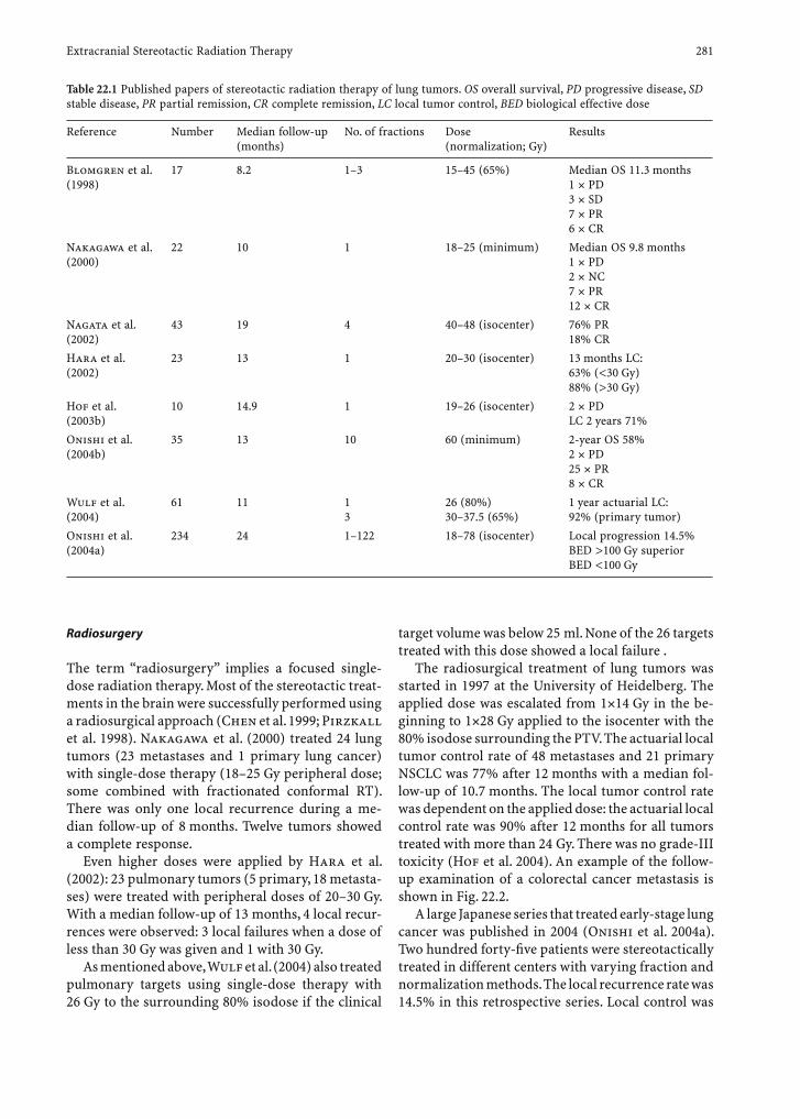
Extracranial Stereotactic Radiation Therapy 281

Radiosurgery

The term “radiosurgery” implies a focused single-dose radiation therapy. Most of the stereotactic treat-ments in the brain were successfully performed using a radiosurgical approach (Chen et al. 1999; Pirzkall et al. 1998). Nakagawa et al. (2000) treated 24 lung tumors (23 metastases and 1 primary lung cancer) with single-dose therapy (18–25 Gy peripheral dose; some combined with fractionated conformal RT). There was only one local recurrence during a me-dian follow-up of 8 months. Twelve tumors showed a complete response.

Even higher doses were applied by Hara et al. (2002): 23 pulmonary tumors (5 primary, 18 metasta-ses) were treated with peripheral doses of 20–30 Gy. With a median follow-up of 13 months, 4 local recur-rences were observed: 3 local failures when a dose of less than 30 Gy was given and 1 with 30 Gy.

As mentioned above, Wulf et al. (2004) also treated pulmonary targets using single-dose therapy with 26 Gy to the surrounding 80% isodose if the clinical

target volume was below 25 ml. None of the 26 targets treated with this dose showed a local failure .

The radiosurgical treatment of lung tumors was started in 1997 at the University of Heidelberg. The applied dose was escalated from 1×14 Gy in the be-ginning to 1×28 Gy applied to the isocenter with the 80% isodose surrounding the PTV. The actuarial local tumor control rate of 48 metastases and 21 primary NSCLC was 77% after 12 months with a median fol-low-up of 10.7 months. The local tumor control rate was dependent on the applied dose: the actuarial local control rate was 90% after 12 months for all tumors treated with more than 24 Gy. There was no grade-III toxicity (Hof et al. 2004). An example of the follow-up examination of a colorectal cancer metastasis is shown in Fig. 22.2.

A large Japanese series that treated early-stage lung cancer was published in 2004 (Onishi et al. 2004a). Two hundred forty-fi ve patients were stereotactically treated in different centers with varying fraction and normalization methods. The local recurrence rate was 14.5% in this retrospective series. Local control was

Table 22.1 Published papers of stereotactic radiation therapy of lung tumors. OS overall survival, PD progressive disease, SD stable disease, PR partial remission, CR complete remission, LC local tumor control, BED biological effective dose

Reference Number Median follow-up (months)

No. of fractions Dose (normalization; Gy)

Results

Blomgren et al. (1998)

17 8.2 1–3 15–45 (65%) Median OS 11.3 months1 × PD3 × SD7 × PR6 × CR

Nakagawa et al. (2000)

22 10 1 18–25 (minimum) Median OS 9.8 months1 × PD2 × NC7 × PR12 × CR

Nagata et al. (2002)

43 19 4 40–48 (isocenter) 76% PR18% CR

Hara et al. (2002)

23 13 1 20–30 (isocenter) 13 months LC:63% (<30 Gy)88% (>30 Gy)

Hof et al. (2003b)

10 14.9 1 19–26 (isocenter) 2 × PDLC 2 years 71%

Onishi et al. (2004b)

35 13 10 60 (minimum) 2-year OS 58%2 × PD25 × PR8 × CR

Wulf et al. (2004)

61 11 13

26 (80%)30–37.5 (65%)

1 year actuarial LC:92% (primary tumor)

Onishi et al. (2004a)

234 24 1–122 18–78 (isocenter) Local progression 14.5%BED >100 Gy superiorBED <100 Gy

282 K. K. Herfarth

signifi cantly better when a biological effective dose (BED) of more than 100 Gy was applied. Three-year survival was 88.4% in medically operable patients if treated with a BED >100 Gy (Onishi et al. 2004a).

Focal Lung Reaction

Radiation pneumonitis is a known phenomenon af-ter conventional fractionated radiotherapy. The term “pneumonopathy” might be better since there is no infective process in place. The rate of clinical symp-tomatic pneumonopathy is dependent on the radiated volume and the dose. It usually occurs 1–3 months after completion of thoracic irradiation. Recovery from so-called pneumonitis usually occurs and a fi brosis follows and progresses in time. Symptoms may involve low-grade fever, congestion, cough, full-ness in the chest, and also dyspnea and chest pain. Radiological changes involve a homogenous increase in radiodensity and patchy, discrete, or solid consoli-dation with varying time tables, appearing weeks to years after radiotherapy corresponding to the acute pneumonitis and the chronic fi brosis phases.

The same pattern of focal lung reaction have also been seen after stereotactic radiation therapy of lung tumors. Takeda et al. (2004) described ground-glass opacities in 18% of hypofractionated treated tumors and dense consolidation in 73%. We have found changes in 80% of all tumors treated with 24 Gy single dose or more (Herfarth et al. 2000a). On the other hand, the rate of clinically symptomatic radia-tion pneumonopathy is low due to the small volumes irradiated. The shape of the resulting consolidating fi brosis might change over years and should not be falsely diagnosed as local recurrence (Wulf et al. 2001). Many questions remain unanswered: Which

factors infl uence the pattern and the occurrence of the pneumonopathy? Is there a threshold dose? Can we predict radiation pneumonitis using the mean lung dose? There are several trials underway which should give answers to these questions.

22.4.2 Liver

Hypofractionation

Blomgren et al. were the fi rst authors to publish data about stereotactic irradiation of liver tumors. Their initial report in 1995 was followed by an update in 1998 (Blomgren et al. 1995, 1998). After having had negative experiences with single-dose therapy, which is discussed later, they mainly used hypofraction-ated radiotherapy. The fractionation and the over-all time of treatment were very variable. The dose ranged from 2×8 to 3×15 Gy or 4×10 Gy. The dose was prescribed to the PTV compassing 65% isodose, which resulted in maximal total doses of 20–82 Gy. The treatment time varied between 3 and 44 days (Blomgren et al. 1998).

Blomgren et al. (1995, 1998) treated 20 primary intrahepatic cancers in 11 patients. The clinical target volume was median 22 cc with a range of 3–622 cc. With a mean follow-up of 12 months, they described no local failure; however, two cases of radiation-in-duced liver disease (RILD) with fatal ending were reported. Both patients had liver cirrhosis. The fi rst patient presented with a 57-cc hepatocellular car-cinoma (HCC) nodule due to hepatitis C and liver cirrhosis. The tumor was treated with 3×15 Gy to the periphery of the PTV. The patient developed as-

Fig. 22.2 Lung metastasis of a colorectal cancer before radiosurgical treatment (left) and 7 months after treatment (right)

Extracranial Stereotactic Radiation Therapy 283

cites 20 days after completion of the treatment and died the next month. The other patient had a 293-cc large HCC treated with 3×10 Gy to the periphery of the PTV. Also this patient developed non-tractable ascites in the fi rst 6 weeks after treatment and died shortly after that. Unfortunately, there is no detailed information about the size of the liver, the degree of pretherapeutic liver impairment, or the mean liver dose; therefore, no defi nite conclusions about the risk assessment can be drawn from this published data. Apart from these fatal side effects, patients ex-perienced nausea, fever, or chills for a few hours after radiosurgery.

Ten patients with 20 metastases were also treated at the Karolinska Institute using the hypofraction-ated stereotactic regimen. The median CTV was 24 cc with a range of 2–263 cc. Tumor response was evaluated after a mean follow-up time of 9.6 months. All tumors showed response to the therapy. One lo-cal recurrence was observed 6 months after therapy. Again, patients experienced nausea, fever, and chill a few hours after the procedure. These symptoms were handled with a prophylactic treatment with paracetamol and antiemetics later. One patient suf-fered from a hemorrhagic gastritis a few weeks after treatment. One third of the stomach wall had been exposed to 7 Gy for two treatment sessions. Parts of the duodenum were exposed to 4×5 Gy in another pa-tient. This patient developed a duodenal ulcer, which was treated conservatively.

These early Stockholm data indicated the feasibil-ity and the possible success rate of a hypofractionated stereotactic treatment of liver tumors. Unfortunately, no dose-volume-success constraints can be drawn from these data due to the wide range of the ap-plied dose and different fractionation schemes. The Stockholm group has continued to treat patients with hepatic cancer with the stereotactic approach; how-ever, new data have not been published.

Wulf et al. (2001), from the University of Würzburg (Germany) adopted parts of the Stockholm treat-ment approach . They treated 24 patients with liver tumors (one clear cell carcinoma and 23 metastases). The median clinical target volume was 50 cc with a minimum of 9 cc and a maximum of 512 cc. All but one patient were treated with 3×10 Gy to the 65% isodose at the periphery of the PTV. One patient was treated by 4×7 Gy also normalized to the periphery of the PTV. The reason for this other fractionation was a close proximity of the target to the esophagus. The crude local control was 83% with a mean follow-up of 9 months. The actuarial local control after 12 months was reported with 76%. The recurrences occurred 3,

8, 9, and 17 months after treatment. All were treated with 3×10 Gy. The failures of three of these targets occurred marginally. The median survival of these patients was calculated to 20 months. The morbidity of the treatment was low: only 7 of 24 patients re-ported side effects of grades 1 or 2 according to the WHO classifi cation. The side effects were mostly re-lated only to one fraction and included fever, chills, or pain with a typical onset a few hours after irradiation. Additionally, nausea and/or vomiting might occur at the same time. The symptoms ceased spontaneously or could successfully be treated with paracetamol or prednisolone. Only one patient showed longer-last-ing fatigue, weakness, and loss of appetite.

Radiosurgery

Blomgren et al. (1998) also started with a single dose therapy for liver tumors. Six tumors in 5 patients were radiosurgically treated. The prescribed dose to the periphery of the PTV was median 15.5 Gy rang-ing from 7.7 to 30 Gy. No recurrences were observed during a median follow-up of 5 months; however, one patient died 2 days after treatment. These patients had a 229-cc large HCC in a cirrhotic liver. The tumor was treated with 30 Gy applied to the periphery of the PTV. The isocenter dose was 48 Gy. The patient already was icteric and showed signs of ascites at the time of treatment. The other four patients showed marginal recurrences during follow-up as is men-tioned in a later paper by Blomgren et al. (1998). These two circumstances forced Blomgren et al. to abandon the radiosurgical approach for large liver tumors.

In 1997, a phase-I/II trial was initiated at the German Cancer Research Center in Heidelberg (Germany) proving the feasibility and the clinical outcome of a single-dose radiation therapy of liver tumors (Herfarth et al. 2001a). Inclusion crite-ria for the study were non-resectable tumors in the liver. The number of liver lesions was not to exceed three tumors (four, if two tumors <3 cm were close together). The size of a single lesion was not to exceed 6 cm, and none of the tumors could be immediately adjacent to parts of the gastrointestinal tract (dis-tance >6 mm). Exclusion criteria were an insuffi cient liver function. Thirty-seven patients were included. A total of 60 tumors were radiosurgically treated on 40 occasions. The targets included 4 primary hepatic tumors and 56 metastases (mainly colorectal cancer or breast cancer). The median target size was 10 cc (range 1–132 cc). The dose was prescribed to the iso-center with the 80% isodose encompassing the PTV.

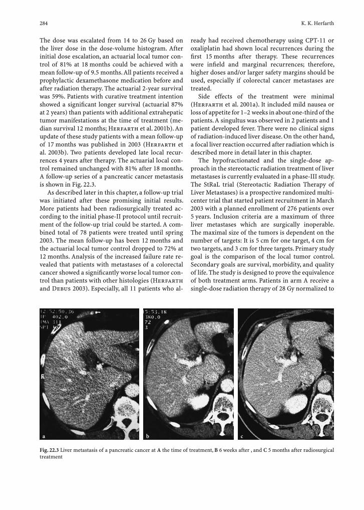
284 K. K. Herfarth

The dose was escalated from 14 to 26 Gy based on the liver dose in the dose-volume histogram. After initial dose escalation, an actuarial local tumor con-trol of 81% at 18 months could be achieved with a mean follow-up of 9.5 months. All patients received a prophylactic dexamethasone medication before and after radiation therapy. The actuarial 2-year survival was 59%. Patients with curative treatment intention showed a signifi cant longer survival (actuarial 87% at 2 years) than patients with additional extrahepatic tumor manifestations at the time of treatment (me-dian survival 12 months; Herfarth et al. 2001b). An update of these study patients with a mean follow-up of 17 months was published in 2003 (Herfarth et al. 2003b). Two patients developed late local recur-rences 4 years after therapy. The actuarial local con-trol remained unchanged with 81% after 18 months. A follow-up series of a pancreatic cancer metastasis is shown in Fig. 22.3.

As described later in this chapter, a follow-up trial was initiated after these promising initial results. More patients had been radiosurgically treated ac-cording to the initial phase-II protocol until recruit-ment of the follow-up trial could be started. A com-bined total of 78 patients were treated until spring 2003. The mean follow-up has been 12 months and the actuarial local tumor control dropped to 72% at 12 months. Analysis of the increased failure rate re-vealed that patients with metastases of a colorectal cancer showed a signifi cantly worse local tumor con-trol than patients with other histologies (Herfarth and Debus 2003). Especially, all 11 patients who al-

ready had received chemotherapy using CPT-11 or oxaliplatin had shown local recurrences during the fi rst 15 months after therapy. These recurrences were infi eld and marginal recurrences; therefore, higher doses and/or larger safety margins should be used, especially if colorectal cancer metastases are treated.

Side effects of the treatment were minimal (Herfarth et al. 2001a). It included mild nausea or loss of appetite for 1–2 weeks in about one-third of the patients. A singultus was observed in 2 patients and 1 patient developed fever. There were no clinical signs of radiation-induced liver disease. On the other hand, a focal liver reaction occurred after radiation which is described more in detail later in this chapter.

The hypofractionated and the single-dose ap-proach in the stereotactic radiation treatment of liver metastases is currently evaluated in a phase-III study. The StRaL trial (Stereotactic Radiation Therapy of Liver Metastases) is a prospective randomized multi-center trial that started patient recruitment in March 2003 with a planned enrollment of 276 patients over 5 years. Inclusion criteria are a maximum of three liver metastases which are surgically inoperable. The maximal size of the tumors is dependent on the number of targets: It is 5 cm for one target, 4 cm for two targets, and 3 cm for three targets. Primary study goal is the comparison of the local tumor control. Secondary goals are survival, morbidity, and quality of life. The study is designed to prove the equivalence of both treatment arms. Patients in arm A receive a single-dose radiation therapy of 28 Gy normalized to

Fig. 22.3 Liver metastasis of a pancreatic cancer at A the time of treatment, B 6 weeks after , and C 5 months after radiosurgical treatment

ba c

Extracranial Stereotactic Radiation Therapy 285

the isocenter with the 80% isodose (22.4 Gy) encom-passing the PTV. Patients in arm B receive a hypo-fractionated therapy with 3×12.5 Gy normalized to the 65% isodose (encompassing the PTV).

Focal Liver Reaction

The focal liver reaction after single-dose radiation therapy has been examined by the Heidelberg group. All patients who were followed using multiphasic CT scanning showed a sharply demarcated focal radia-tion reaction. Tumor and radiation reaction could be well differentiated in the portal-venous contrast-enhanced CT scans. Liver vessels run through the liver reaction and were not displaced, as is seen in cases of expanding tumor. A detailed evaluation and characterization of this focal radiation reaction in 36 of the Heidelberg patients was published in 2003 (Herfarth et al. 2003a).

The area of radiation reaction was hypodense in the majority of the non-enhanced CT scans. Three different types of appearance of the reaction could be defi ned based on the liver density in the portal-venous and the late phase after contrast agent admin-istration:1. Type-1 reaction: Hypodensity in portal-venous

contrast phase, isodensity in the late contrast phase

2. Type-2 reaction: Hypodensity in portal-venous contrast phase, hyperdensity in the late contrast phase

3. Type-3 reaction: Isodensity/hyperdensity in portal-venous contrast phase, hyperdensity in the late contrast phase

The onset of the reaction was after median 1.8 months. While the type-1 or type-2 reactions usu-ally showed up earlier, type-3 reactions appeared later than the other types. It was also seen that there was a shift of the appearance during follow-up towards type-3 appearances. In addition, the volume of the ra-diation reaction decreased with follow-up time. The most dramatic shrinkage was observed during the fi rst months after appearance. This led to the specu-lation that the whole reaction goes through different radiological stages (type 1, 2, and 3 appearances). The histological basis of these stages was not deter-mined since no biopsies were taken; however, others had reported a type-2 appearance after single-dose radiation therapy and it was histologically confi rmed veno-occlusive disease (Willemart et al. 2000).

Based on reconstruction of the dose-volume his-tograms, the mean threshold dose was 13.7 Gy with a

wide range between 8.9 and 19.2 Gy given in a single fraction. One reason for this large variance might be the fact that the volume strongly decreased between the initial detection and the further follow-up exam-inations. The examination might have not detected larger reaction volumes and, therefore, the calculated threshold doses might have been overestimated. This was sustained by the signifi cant correlation between the threshold dose and the time of detection (corre-lation coeffi cient r=0.709). Apart of the time factor, other factors, which might infl uence the individual radiation sensitivity (e.g., additional toxic liver agents such as alcohol) might have been another reason for the variance. More data are needed to strengthen these threshold doses.

22.4.3 Spinal and Paraspinal Tumors

In opposite to the lung and the liver with a pro-nounced volume effect, the myelon is characterized by a serial function structure: the side effects are more infl uenced by the dose maximum than by the volume treated. The goal for a stereotactic treatment of spinal and paraspinal tumors is to reduce the total dose to the myelon. Figure 22.4 shows a stereotac-tic treatment plan which allows a dose escalation of paraspinal regions with a dose limitation to the spinal

Fig. 22.4 Dose distribution for a fractionated stereotactic radi-ation treatment of a paraspinal sarcoma. The dose to the spinal cord is limited if the stereotactic setup ensures a precise repo-sition. The orange area marks the 60–80% isodose fall-off

286 K. K. Herfarth

chord. Again, there have been different stereotactic approaches to achieve that goal: single-dose therapy and fractionation. What they have in common is a greater effort in positioning of the patient.

Fractionated Stereotactic Treatment

We treated 18 patients with 19 recurrent spinal me-tastases using a normofractionated stereotactic ap-proach (Milker-Zabel et al. 2003). All patients had previous irradiation of the tumors with a median dose of 38 Gy. The median reirradiation dose was 39 Gy in 1.8- to 2-Gy fractions. The dose to the spinal chord was limited to less than 20 Gy in all patients The positioning accuracy was provided using a whole-body cast which guarantees an optimal repositioning of the spine using a non-invasive method (Lohr et al. 1999). Of the patients, 95% showed radiological response after a median follow-up of 12.3 months. There were no signs of radiation-induced myelotox-icity (Milker-Zabel et al. 2003).

Radiosurgery

Hamilton et al. (1995) used an invasive fi xation of the patient. The patient’s spine was rigidly fi xed to the stereotactic frame while the patient was under general anesthesia. The fi rst experience included 5 patients who already had normal fractionated radia-tion therapy to the spinal cord. They again stereo-tactically delivered 8–10 Gy to the recurrent tumor, which was near the myelon. None of the patients showed a spinal chord injury with a median follow-up of 6 months .

Gerszten et al. (2004) reported on the clinical ex-perience in the radiosurgical treatment of 125 spinal lesions using the CyberKnife. Of the patients, 78% had received radiation treatment of treated region previously. The tumors were treated with a median dose of 14 Gy to 80% isodose line (range 12–20 Gy) and a maximal dose of 8 Gy was allowed to the spi-nal canal; however, the maximum dose to the edge of the spinal canal was 13 Gy in a single patient. With a median follow-up of 18 months, none of the patients experienced exacerbation of the symptoms or new neurological defi cits. Nearly all patients who suffered from pain described an improvement .

Ryu et al. (2003) described 10 patients who re-ceived 10×2.5 Gy via standard external beam radio-therapy. The tumors were additionally treated with an image-based radiosurgical boost of 6–8 Gy, pre-scribed to the 90% isodose line. The maximum dose of radiation to the anterior edge of the spinal cord

within a transverse section, on average, was 50% of the prescribed dose. There was no acute radiation toxicity detected clinically; however, the mean fol-low-up was only 6 months.

22.5 Conclusion

Stereotactic radiation treatment of extracranial tar-gets shows promising initial results. The techniques are getting increasingly more specialized, especially in the treatment of small lung tumors; however, many questions remain unanswered. More experimental work and clinical trials are underway which should answer these question and should strengthen this promising approach.

References

Blomgren H, Lax I, Näslund I et al. (1995) Stereotactic high dose fraction radiation therapy of extracranial tumors using an accelerator. Acta Oncol 34:861–870

Blomgren H, Lax I, Göranson H et al. (1998) Radiosurgery for tumors in the body: clinical experience using a new method. J Radiosurg 1:63–74

Chang SD, Main W, Martin DP et al. (2003) An analysis of the accuracy of the CyberKnife: a robotic frameless stereotac-tic radiosurgical system. Neurosurgery 52:140–147

Chen JC, O’Day S, Morton D et al. (1999) Stereotactic radio-surgery in the treatment of metastatic disease to the brain. Stereotact Funct Neurosurg 73:60–63

Dawson LA, Brock KK, Kazanjian S et al. (2001) The repro-ducibility of organ position using active breathing control (ABC) during liver radiotherapy. Int J Radiat Oncol Biol Phys 51:1410–1421

Dienemann H, Hof H, Debus J et al. (2004) Lungenmetastasen. Onkologe 10:458–473

Dosoretz DE, Galmarini D, Rubenstein JH et al. (1993) Local control in medically inoperable lung cancer: an analysis of its importance in outcome and factors determining the probability of tumor eradication. Int J Radiat Oncol Biol Phys 27:507–516

Fuss M, Salter BJ, Rassiah P et al. (2004) Repositioning accu-racy of a commercially available double-vacuum whole body immobilization system for stereotactic body radia-tion therapy. Technol Cancer Res Treat 3:59–67

Gerszten PC, Ozhasoglu C, Burton SA et al. (2004) CyberKnife frameless stereotactic radiosurgery for spinal lesions: clini-cal experience in 125 cases. Neurosurgery 55:89–99

Hamilton AJ, Lulu BA (1995) A prototype device for linear accelerator-based extracranial radiosurgery. Acta Neuro-chir Suppl (Wien) 63:40–43

Hamilton AJ, Lulu BA, Fosmire A et al. (1995) Preliminary clinical experience with linear accelerator-based spinal stereotactic radiosurgery. Neurosurgery 36:311–319

Extracranial Stereotactic Radiation Therapy 287

Hamilton AJ, Lulu BA, Fosmire H et al. (1996) LINAC-based spinal stereotactic radiosurgery. Stereotact Funct Neuro-surg 66:1–9

Hanley J, Debois MM, Mah D et al. (1999a) Deep inspiration breath-hold technique for lung tumors: the potential value of target immobilization and reduced lung density in dose escalation. Int J Radiat Oncol Biol Phys 45:603–611

Hanley J, Debois MM, Mah M et al. (1999b) Deep inspiration breath-hold technique for lung tumors: the potential value of target immobilization and reduced lung density in dose escalation. Int J Radiat Oncol Biol Phys 45:603–611

Hara R, Itami J, Kondo T et al. (2002) Stereotactic single high dose irradiation of lung tumors under resperitory gating. Radiother Oncol 63:159–163

Hartmann GH, Schlegel W, Sturm V et al. (1985) Cerebral radia-tion surgery using moving fi eld irradiation at a linear accel-erator facility. Int J Radiat Oncol Biol Phys 11:1185–1192

Hayakawa K, Mitsuhashi N, Saito Y (1999) Limited fi eld irra-diation for medically inoperable patients with peripheral stage I non-small cell lung cancer. Lung Cancer 26:137–142

Herfarth KK, Debus J (2003) Stereotactic radiation therapy of liver tumors. Radiother Oncol 68 (Suppl 1):S45

Herfarth KK, Debus J, Lohr F et al. (2000a) Stereotactic single dose radiation treatment of tumors in the lung. Radiology 217 (Suppl):148

Herfarth KK, Debus J, Lohr F et al. (2000b) Extracranial ste-reotactic radiation therapy: set-up accuracy of patients treated for liver metastases. Int J Radiat Oncol Biol Phys 46:329–335

Herfarth KK, Pirzkall A, Lohr F et al. (2000c) Erste Erfahrun-gen mit einem nicht-invasiven Patientenfi xierungssystem für die stereotaktische Strahlentherapie der Prostata. Strahlenther Onkol 176:217–222

Herfarth KK, Debus J, Lohr F et al. (2001a) Stereotactic single dose radiation therapy of liver tumors: results of a phase I/II trial. J Clin Oncol 19:164–170

Herfarth KK, Debus J, Lohr F et al. (2001b) Stereotaktische Bestrahlung von Lebermetastasen. Radiologe 41:64–68

Herfarth KK, Hof H, Bahner ML et al. (2003a) Assessment of focal liver reaction by multiphasic CT after stereotactic single-dose radiotherapy of liver tumors. Int J Radiat Oncol Biol Phys 57:444–451

Herfarth KK, Münter MW, Debus J (2003b) Strahlentherapeu-tische Behandlung von Lebermetastasen. Chir Gastroen-terol 19:359-363

Hof H, Herfarth KK, Munter M et al. (2003a) The use of the multislice CT for the determination of respiratory lung tumor movement in stereotactic single-dose irradiation. Strahlenther Onkol 179:542–547

Hof H, Herfarth KK, Munter M et al. (2003b) Stereotactic single-dose radiotherapy of stage I non-small-cell lung cancer (NSCLC). Int J Radiat Oncol Biol Phys 56:335–341

Hof H, Herfarth K, Wannenmacher M et al. (2004) Stereo-taktische Bestrahlung von Lungentumoren: Erfahrungen mit einem Einzeitkonzept. Strahlenther Onkol 180 (Suppl 1):17

International Registry of Lung Metastases (1997) Long-term results of metastasectomy: prognostic analyses based on 5206 cases. J Thorac Cardiovasc Surg 113:37–49

Koong AC, Le QT, Ho A et al. (2004) Phase I study of stereotac-tic radiosurgery in patients with locally advanced pancre-atic cancer. Int J Radiat Oncol Biol Phys 58:1017–1021

Lax I, Blomgren H, Näslund I et al. (1994) Stereotactic radio-therapy of malignancies in the abdomen. Acta Oncol 33:677–683

Leksell L (1951) The stereotactic method and radiosurgery of the brain. Acta Chir Scand 102:316–319

Lohr F, Debus J, Frank C et al. (1999) Noninvasive patient fi xa-tion for extracranial stereotactic radiotherapy. Int J Radiat Oncol Biol Phys 45:521–527

Mageras GS, Yorke E (2004) Deep inspiration breath hold and respiratory gating strategies for reducing organ motion in radiation treatment. Semin Radiat Oncol 14:65–75

Milker-Zabel S, Zabel A, Thilmann C et al. (2003) Clinical results of retreatment of vertebral bone metastases by ste-reotactic conformal radiotherapy and intensity-modulated radiotherapy. Int J Radiat Oncol Biol Phys 55:162–167

Minohara S, Kanai T, Endo M et al. (2000) Respiratory gated irradiation system for heavy-ion radiotherapy. Int J Radiat Oncol Biol Phys 47:1097–1103

Nagata Y, Negoro Y, Aoki T et al. (2002) Clinical outcomes of 3D conformal hypofractionated single high-dose radiotherapy for one or two lung tumors using a stereotactic body frame. Int J Radiat Oncol Biol Phys 52:1041–1046

Nakagawa K, Aoki Y, Tago M et al. (2000) Megavoltage CT-assisted stereotactic radiosurgery for thoracic tumors: original reseach in the treatment of thoracic neoplasms. Int J Radiat Oncol Biol Phys 48:449–457

Onishi H, Kuriyama K, Komiyama T et al. (2003) CT evalua-tion of patient deep inspiration self-breath-holding: How precisely can patients reproduce the tumor position in the absence of respiratory monitoring devices? Med Phys 30:1183–1187

Onishi H, Araki T, Shirato H et al. (2004a) Stereotactic hypo-fractionated high-dose irradiation for stage I nonsmall cell lung carcinoma: clinical outcomes in 245 subjects in a Japa-nese multiinstitutional study. Cancer 101:1623–1631

Onishi H, Kuriyama K, Komiyama T et al. (2004b) Clinical out-comes of stereotactic radiotherapy for stage I non-small cell lung cancer using a novel irradiation technique: patient self-controlled breath-hold and beam switching using a combination of linear accelerator and CT scanner. Lung Cancer 45:45–55

Pirzkall A, Debus J, Lohr F et al. (1998) Radiosurgery alone or in combination with whole-brain radiotherapy for brain metastases. J Clin Oncol 16:3563–3569

Rosenzweig KE, Hanley J, Mah D et al. (2000) The deep inspira-tion breath-hold technique in the treatment of inoperable non-small-cell lung cancer. Int J Radiat Oncol Biol Phys 48:81–87

Ryu S, Fang Yin F, Rock J et al. (2003) Image-guided and intensity-modulated radiosurgery for patients with spinal metastasis. Cancer 97:2013–2018

Starkschall G, Forster KM, Kitamura K et al. (2004) Correla-tion of gross tumor volume excursion with potential ben-efi ts of respiratory gating. Int J Radiat Oncol Biol Phys 60:1291–1297

Takeda T, Takeda A, Kunieda E et al. (2004) Radiation injury after hypofractionated stereotactic radiotherapy for peripheral small lung tumors: serial changes on CT. Am J Roentgenol 182:1123–1128

Thilmann C, Schulz-Ertner D, Zabel A et al. (2002) Intensity-modulated radiotherapy of sacral chordoma: a case report and a comparison with stereotactic conformal radiother-apy. Acta Oncol 41:395–399

288 K. K. Herfarth

Timmerman R, Papiez L, McGarry R et al. (2003) Extracra-nial stereotactic radioablation: results of a phase I study in medically inoperable stage I non-small cell lung cancer. Chest 124:1946–1955

Uematsu M, Shioda A, Tahara K et al. (1998) Focal, high dose, and fractionated modifi ed stereotactic radiation therapy for lung carcinoma patients. Cancer 82:1062–1070

Warner MA, Warner ME, Buck CF et al. (1988) Clinical effi -cacy of high frequency jet ventilation during extracorporal shock wave lithotripsy of renal and ureteral calculi: a com-parison with conventional mechanical ventilation. J Urol 139:486–487

Willemart S, Nicaise N, Struyven J et al. (2000) Acute radiation-induced hepatic injury: evaluation by triphasic contrast enhanced helical CT. Br J Radiol 73:544–546

Wong J, Sharpe M, Jaffray D et al. (1999) The use of active breathing control (ABC) to reduce margin for breathing motion. Int J Radiat Oncol Biol Phys 44:911–919

Wulf J, Hädinger U, Oppitz U et al. (2000) Stereotactic radio-therapy of extracranial targets: CT-simulation and accu-racy of treatment in the stereotactic body frame. Radiother Oncol 57:225–236

Wulf J, Hädinger U, Oppitz U et al. (2001) Stereotactic radio-therapy of targets in the lung and liver. Strahlenther Onkol 177:645–655

Wulf J, Haedinger U, Oppitz U et al. (2004) Stereotactic radio-therapy of primary lung cancer and pulmonary metastases: a non-invasive treatment approach in medically inoperable patients. Int J Radiat Oncol Biol Phys 60:186–196

Yin F, Kim JG, Haughton C et al. (2001) Extracranial radio-surgery: immobilizing liver motion in dogs using high-fre-quency jet ventilation and total intravenous anesthesia. Int J Radiat Oncol Biol Phys 49:211–216

Zierhut D, Bettscheider C, Schubert K et al. (2001) Radia-tion therapy of stage I and II non-small cell lung cancer (NSCLC). Lung Cancer 34 (Suppl) 3:S39–S43

X-IMRT 289

23 X-IMRT

Simeon Nill, Ralf Hinderer, and Uwe Oelfke

S. Nill, PhD; R. Hinderer, PhD; U. Oelfke, PhDAbteilung Medizinische Physik in der Strahlentherapie, Deutsches Krebsforschungszentrum, Im Neuenheimer Feld 280, 69120 Heidelberg, Germany

23.1 Introduction

The IMRT dose delivery techniques are the second cornerstone of X-IMRT in addition to the concepts of inverse treatment planning and optimization (dis-cussed in Chap. 17). The result of an inverse treat-ment plan usually consists of ideal photon-fl uence distributions for each selected beam angle. In this chapter we discuss on a very fundamental level the main concepts and strategies for the actual delivery of these fl uence patterns to a patient. This very brief summary of some of the interesting techniques can-not be complete and very detailed. The interested reader who aims to explore the touched topics in more depth is referred to the standard literature, e.g., Webb (2001) or (Palta and Mackie 2003).

The main focus in this chapter is on the discussion of the most prominent dose delivery techniques with linac-integrated multi-leaf collimators (MLCs). The

basic concepts employed for the two standard meth-ods – the “step-and-shoot” approach and the “dy-namic” dose delivery – are briefl y reviewed before the new concept of “helical tomography” is introduced. Finally, a short section describes the dose delivery technique with individually designed compensators.

23.2 MLC-based IMRT Delivery

Most modern linear accelerators are equipped with MLCs, which were originally designed to replace the use of lead blocks to shield normal tissue during the treatment (Biggs et al. 1991; Boesecke et al. 1991; Jordan and Williams 1994). In the next section we fi rst describe the main IMRT relevant characteristics of a typical MLC including its dosimetric properties. Then, various dose delivery techniques are briefl y de-scribed. Based on the MLC computer-control system, two main dose delivery methods are distinguished: (a) the “step-and-shoot” approach; and (b) the “dy-namic” dose delivery concept. A very detailed de-scription of both techniques with references to the original papers can be found in the excellent book by Webb (2001). Besides these two basic IMRT delivery concepts with linac-integrated MLCs, we also briefl y discuss some examples of “high-resolution” IMRT with add-on mini- or micro-MLCs.

23.2.1 MLC Design

23.2.1.1 IMRT-Relevant MLC Data

Multi-leaf collimators and their design and func-tion for 3D conformal radiotherapy (3D CRT) are described in detail in Chap. 20, together with their geometrical and mechanical characteristics, see also Galvin et al. (19939.

CONTENTS

23.1 Introduction 28923.2 MLC-based IMRT Delivery 28923.2.1 MLC Design 28923.2.1.1 IMRT-Relevant MLC Data 28923.2.2 Step-and-Shoot Dose Delivery 29023.2.2.1 The Step-and-Shoot Technique 29023.2.2.2 Leaf-Sequencing Algorithms 29023.2.2.3 Hardware Constraints: Matchlines 29223.2.3 Dynamic Dose Delivery 29223.2.4 Improved Spatial Resolution: Add-on MLCs 29423.3 Helical Tomotherapy Delivery 29523.4 Compensator-Based IMRT Delivery 296 References 297

290 S. Nill et al.

To deliver intensity-modulated fi elds (IMRT) the following geometric characteristics are of most im-portance:

1. Leaf width. The leaf width (see Chap. 20.2.1) determines one dimension of the achievable spa-tial resolution of the fl uence modulation. The spatial resolution of the fl uence in the direction of the leaves’ movement is only restricted by the positioning accuracy of the MLC. For the delivery of IMRT fi elds a possible large overtravel range of the different leaves (10–15 cm) is often required to irradiate extended target volumes.

2. Maximum leaf speed. The leaf speed is especially important for the “dynamic” delivery of intensity-modulated fi elds. A typical leaf speed is of the order of 2–4 cm/s (Webb 2001; Hug 2002).

3. The maximum fi eld size of the MLC. For IMRT applications, the maximum fi eld size is not the same as the maximum open fi eld which can be achieved, but it is mainly defi ned by the maximum overtravel.

4. Maximum overtravel. Maximum overtravel (see Chap. 20.2.1) is the distance of how far a leaf can move over the midline of the MLC.

5. Leakage and transmission. The leakage and transmission (see Chaps. 20.2.2.2, 20.2.2.3) play an important role specifi cally for the delivery of IMRT treatments because the dose delivery often requires a substantial number of monitor units (MU); these are applied where most areas of the treatment fi eld are covered with closed leaves, i.e., the leakage radiation received by these areas is signifi cantly enhanced.

6. Leaf-positioning accuracy. One of the most impor-tant properties of an MLC with respect to IMRT is the leaf-positioning accuracy. For IMRT deliv-ery the leaf-positioning accuracy is even more important than for most conventional treatment techniques due to the large number of small fi eld components for an average IMRT treatment. For a typical fl uence grid with a resolution of 10 mm in both directions a leaf-positioning error of 1 mm has to be considered as a large error. This is due to the characteristic output factor curve with a very steep gradient for small fi eld sizes. An error of 1 mm for the leaf position can cause a dose error of up to approximately 10% irradiating a 10×10-mm fi eld and therefore the maximum leaf-positioning error should not be larger than 0.5 mm. It can also be concluded that the required leaf-positioning accuracy depends on the fl uence grid resolution of the fl uence maps.

23.2.2 Step-and-Shoot Dose Delivery

As result of the inverse planning process, described in Chap. 17, one receives the “ideal” fl uence maps for each incident beam direction. In most treatment planning systems these ideal intensity maps have to be converted into fi eld segments to be delivered with the MLC, a process that is called the “sequencing” of the fl uence. In this section we shortly describe the “step-and-shoot” dose delivery method and discuss briefl y the two basic sequencing techniques.

23.2.2.1 The Step-and-Shoot Technique

The “step-and-shoot” technique of IMRT dose de-livery (Bortfeld et al. 1994) is a straightforward extension of the conventional multiple-fi eld irradia-tion technique. The “step-and-shoot” approach su-perimposes the dose delivered by a number of ir-regularly shaped and partially overlapping treatment fi elds, often called subfi elds or segments. For each segment a well-defi ned number of monitor units is delivered. Then, the beam is turned off while the leaves of the MLC move to the positions required by the next IMRT segment. After the verifi cation and record system (V&R) has validated the new leaf posi-tions, the beam is turned on and the dose is delivered for this segment. This process is repeated for all seg-ments per incident beam angle and all beam direc-tions (see Fig. 23.1).

23.2.2.2 Leaf-Sequencing Algorithms

In order to describe the basic features of leaf-sequenc-ing algorithms we introduce the following terms: a fl uence map is defi ned on a 2D fi xed grid covering the respective beam aperture. It is usually divided into discrete, quadratic elements called “bixels.” The fl uence map assigns one beam intensity to each bixel. A 1D line of intensities for all bixels created by a single leaf pair is called a channel. The width of each channel coincides with the leaf width of the MLC. The goal of the sequencing process is to decompose the fl uence maps into a number of fi eld components or subfi elds.

The fi rst step of the sequencing process is the stratifi cation of the continuous fl uence profi les pro-vided by the inverse planning process, i.e., each line of intensity for a specifi c channel is forced to take on only a few discrete fl uence levels (Fig. 23.2). For each

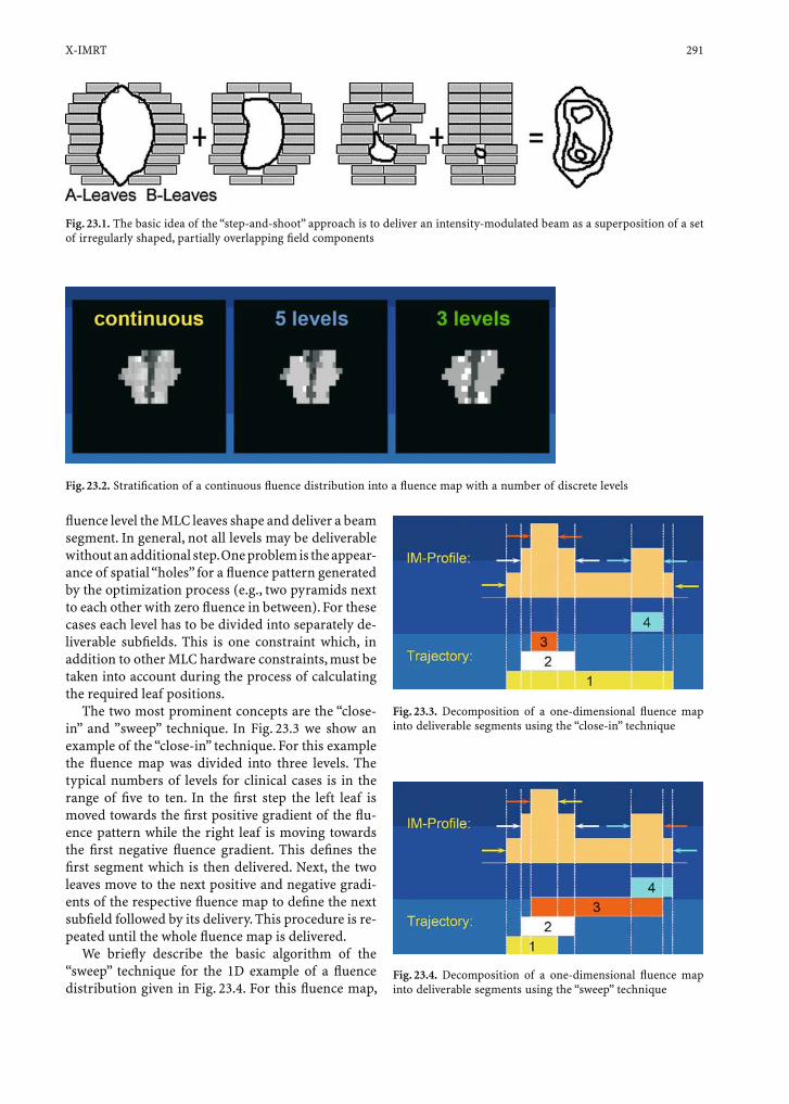
X-IMRT 291

fl uence level the MLC leaves shape and deliver a beam segment. In general, not all levels may be deliverable without an additional step. One problem is the appear-ance of spatial “holes” for a fl uence pattern generated by the optimization process (e.g., two pyramids next to each other with zero fl uence in between). For these cases each level has to be divided into separately de-liverable subfi elds. This is one constraint which, in addition to other MLC hardware constraints, must be taken into account during the process of calculating the required leaf positions.

The two most prominent concepts are the “close-in” and ”sweep” technique. In Fig. 23.3 we show an example of the “close-in” technique. For this example the fl uence map was divided into three levels. The typical numbers of levels for clinical cases is in the range of fi ve to ten. In the fi rst step the left leaf is moved towards the fi rst positive gradient of the fl u-ence pattern while the right leaf is moving towards the fi rst negative fl uence gradient. This defi nes the fi rst segment which is then delivered. Next, the two leaves move to the next positive and negative gradi-ents of the respective fl uence map to defi ne the next subfi eld followed by its delivery. This procedure is re-peated until the whole fl uence map is delivered.

We briefl y describe the basic algorithm of the “sweep” technique for the 1D example of a fl uence distribution given in Fig. 23.4. For this fl uence map,

Fig. 23.1. The basic idea of the “step-and-shoot” approach is to deliver an intensity-modulated beam as a superposition of a set of irregularly shaped, partially overlapping fi eld components

Fig. 23.2. Stratifi cation of a continuous fl uence distribution into a fl uence map with a number of discrete levels

Fig. 23.4. Decomposition of a one-dimensional fl uence map into deliverable segments using the “sweep” technique

Fig. 23.3. Decomposition of a one-dimensional fl uence map into deliverable segments using the “close-in” technique

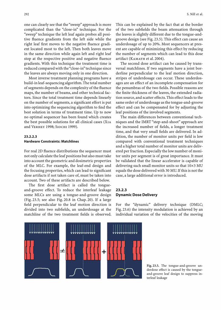
292 S. Nill et al.

one can clearly see that the “sweep” approach is more complicated than the “close-in” technique. For the “sweep” technique the left leaf again probes all posi-tive fl uence gradients from the left side while the right leaf fi rst moves to the negative fl uence gradi-ent located most to the left. Then both leaves move in the same direction while again left and right leaf stop at the respective positive and negative fl uence gradients. With this technique the treatment time is reduced compared with the “close-in” technique since the leaves are always moving only in one direction.

Most inverse treatment planning programs have a build-in leaf-sequencing algorithm. The total number of segments depends on the complexity of the fl uence maps, the number of beams, and other technical fac-tors. Since the total treatment time depends linearly on the number of segments, a signifi cant effort is put into optimizing the sequencing algorithm to fi nd the best solution in terms of treatment time. Up to now no optimal sequencer has been found which creates the best possible solutions for all clinical cases (Xia and Verhey 1998; Siochi 1999).

23.2.2.3 Hardware Constraints: Matchlines

For real 2D fl uence distributions the sequencer must not only calculate the leaf positions but also must take into account the geometric and dosimetric properties of the MLC. For example, the leaf-end design and the focusing properties, which can lead to signifi cant dose artifacts if not taken care of, must be taken into account. Two of these artifacts are described below.

The fi rst dose artifact is called the tongue-and-groove effect. To reduce the interleaf leakage some MLCs are using a tongue-and-groove design (Fig. 23.5; see also Fig. 20.8 in Chap. 20). If a large fi eld perpendicular to the leaf motion direction is divided into two subfi elds, an underdosage at the matchline of the two treatment fi elds is observed.

This can be explained by the fact that at the border of the two subfi elds the beam attenuation through the leaves is slightly different due to the tongue-and-groove design (see Fig. 23.5). This effect can cause an underdosage of up to 20%. Most sequencers at pres-ent are capable of minimizing this effect by reducing the number of segments which can lead to this dose artifact (Kamath et al. 2004).

The second dose artifact can be caused by trans-versal matchlines. If two segments have a joint bor-derline perpendicular to the leaf motion direction, stripes of underdosage can occur. These underdos-ages are an effect of an incomplete compensation for the penumbras of the two fi elds. Possible reasons are the fi nite thickness of the leaves, the extended radia-tion source, and scatter effects. This effect leads to the same order of underdosage as the tongue-and-groove effect and can be compensated for by adjusting the leaf positions of the involved segments.

The main differences between conventional tech-niques and the IMRT “step-and-shoot” approach are the increased number of fi elds, a longer treatment time, and that very small fi elds are delivered. In ad-dition, the number of monitor units per fi eld is low compared with conventional treatment techniques and a higher total number of monitor units are deliv-ered per fraction. Especially the low number of moni-tor units per segment is of great importance. It must be validated that the linear accelerator is capable of delivering such small monitor units so that 10×3 MU equals the dose delivered with 30 MU. If this is not the case, a large additional error is introduced.

23.2.3 Dynamic Dose Delivery

For the “dynamic” delivery technique (DMLC; Fig. 23.6) the intensity modulation is achieved by an individual variation of the velocities of the moving

Fig. 23.5. The tongue-and-groove un-derdose effect is caused by the tongue-and-groove leaf design to suppress in-terleaf leakage

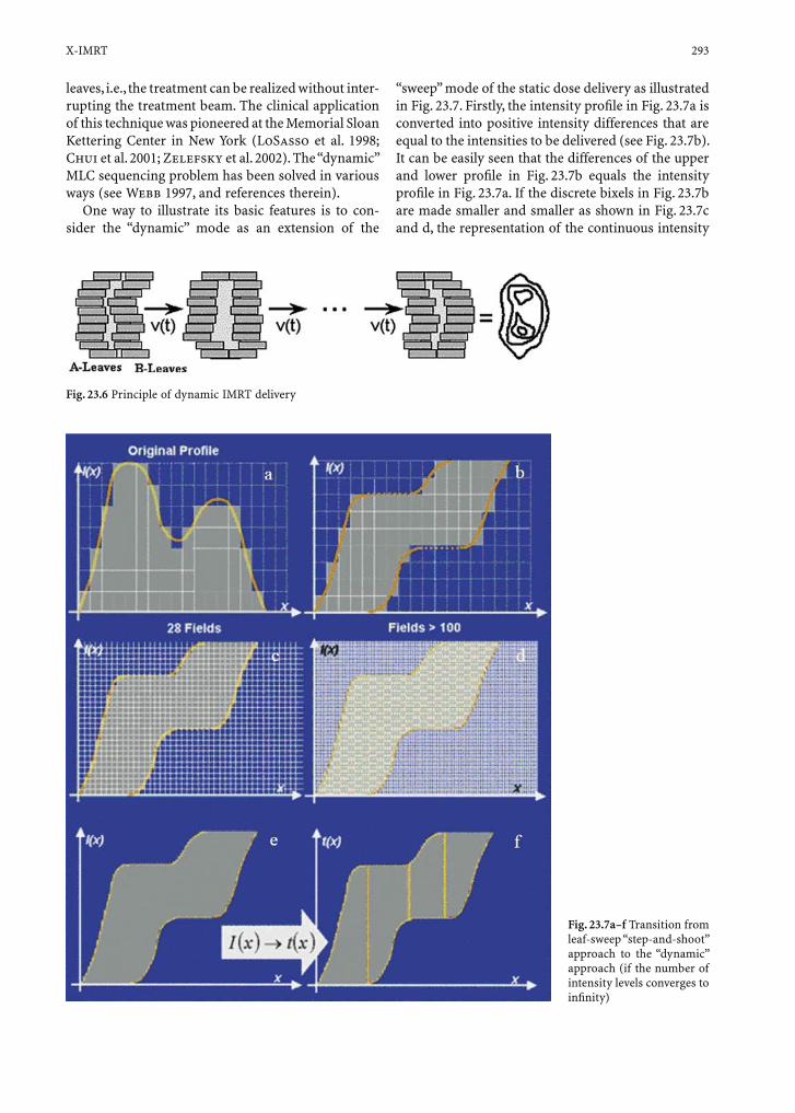
X-IMRT 293

leaves, i.e., the treatment can be realized without inter-rupting the treatment beam. The clinical application of this technique was pioneered at the Memorial Sloan Kettering Center in New York (LoSasso et al. 1998; Chui et al. 2001; Zelefsky et al. 2002). The “dynamic” MLC sequencing problem has been solved in various ways (see Webb 1997, and references therein).

One way to illustrate its basic features is to con-sider the “dynamic” mode as an extension of the

“sweep” mode of the static dose delivery as illustrated in Fig. 23.7. Firstly, the intensity profi le in Fig. 23.7a is converted into positive intensity differences that are equal to the intensities to be delivered (see Fig. 23.7b). It can be easily seen that the differences of the upper and lower profi le in Fig. 23.7b equals the intensity profi le in Fig. 23.7a. If the discrete bixels in Fig. 23.7b are made smaller and smaller as shown in Fig. 23.7c and d, the representation of the continuous intensity

Fig. 23.6 Principle of dynamic IMRT delivery

Fig. 23.7a–f Transition from leaf-sweep “step-and-shoot” approach to the “dynamic” approach (if the number of intensity levels converges to infi nity)

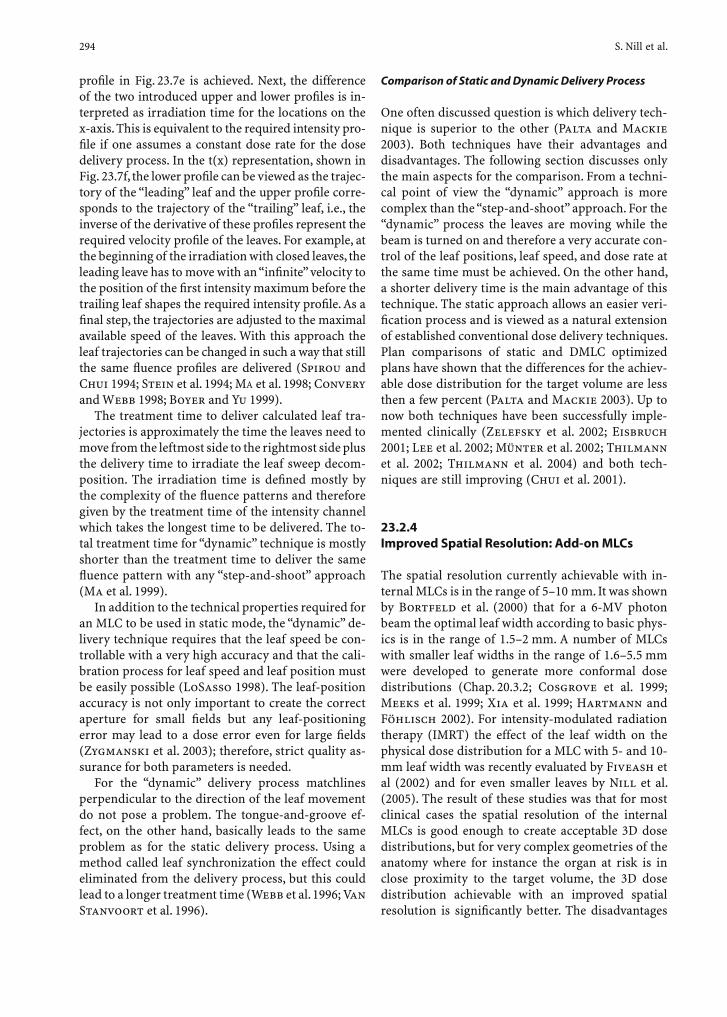
294 S. Nill et al.

profi le in Fig. 23.7e is achieved. Next, the difference of the two introduced upper and lower profi les is in-terpreted as irradiation time for the locations on the x-axis. This is equivalent to the required intensity pro-fi le if one assumes a constant dose rate for the dose delivery process. In the t(x) representation, shown in Fig. 23.7f, the lower profi le can be viewed as the trajec-tory of the “leading” leaf and the upper profi le corre-sponds to the trajectory of the “trailing” leaf, i.e., the inverse of the derivative of these profi les represent the required velocity profi le of the leaves. For example, at the beginning of the irradiation with closed leaves, the leading leave has to move with an “infi nite” velocity to the position of the fi rst intensity maximum before the trailing leaf shapes the required intensity profi le. As a fi nal step, the trajectories are adjusted to the maximal available speed of the leaves. With this approach the leaf trajectories can be changed in such a way that still the same fl uence profi les are delivered (Spirou and Chui 1994; Stein et al. 1994; MA et al. 1998; Convery and Webb 1998; Boyer and Yu 1999).

The treatment time to deliver calculated leaf tra-jectories is approximately the time the leaves need to move from the leftmost side to the rightmost side plus the delivery time to irradiate the leaf sweep decom-position. The irradiation time is defi ned mostly by the complexity of the fl uence patterns and therefore given by the treatment time of the intensity channel which takes the longest time to be delivered. The to-tal treatment time for “dynamic” technique is mostly shorter than the treatment time to deliver the same fl uence pattern with any “step-and-shoot” approach (Ma et al. 1999).

In addition to the technical properties required for an MLC to be used in static mode, the “dynamic” de-livery technique requires that the leaf speed be con-trollable with a very high accuracy and that the cali-bration process for leaf speed and leaf position must be easily possible (LoSasso 1998). The leaf-position accuracy is not only important to create the correct aperture for small fi elds but any leaf-positioning error may lead to a dose error even for large fi elds (Zygmanski et al. 2003); therefore, strict quality as-surance for both parameters is needed.

For the “dynamic” delivery process matchlines perpendicular to the direction of the leaf movement do not pose a problem. The tongue-and-groove ef-fect, on the other hand, basically leads to the same problem as for the static delivery process. Using a method called leaf synchronization the effect could eliminated from the delivery process, but this could lead to a longer treatment time (Webb et al. 1996; Van Stanvoort et al. 1996).

Comparison of Static and Dynamic Delivery Process

One often discussed question is which delivery tech-nique is superior to the other (Palta and Mackie 2003). Both techniques have their advantages and disadvantages. The following section discusses only the main aspects for the comparison. From a techni-cal point of view the “dynamic” approach is more complex than the “step-and-shoot” approach. For the “dynamic” process the leaves are moving while the beam is turned on and therefore a very accurate con-trol of the leaf positions, leaf speed, and dose rate at the same time must be achieved. On the other hand, a shorter delivery time is the main advantage of this technique. The static approach allows an easier veri-fi cation process and is viewed as a natural extension of established conventional dose delivery techniques. Plan comparisons of static and DMLC optimized plans have shown that the differences for the achiev-able dose distribution for the target volume are less then a few percent (Palta and Mackie 2003). Up to now both techniques have been successfully imple-mented clinically (Zelefsky et al. 2002; Eisbruch 2001; Lee et al. 2002; Münter et al. 2002; Thilmann et al. 2002; Thilmann et al. 2004) and both tech-niques are still improving (Chui et al. 2001).

23.2.4 Improved Spatial Resolution: Add-on MLCs

The spatial resolution currently achievable with in-ternal MLCs is in the range of 5–10 mm. It was shown by Bortfeld et al. (2000) that for a 6-MV photon beam the optimal leaf width according to basic phys-ics is in the range of 1.5–2 mm. A number of MLCs with smaller leaf widths in the range of 1.6–5.5 mm were developed to generate more conformal dose distributions (Chap. 20.3.2; Cosgrove et al. 1999; Meeks et al. 1999; Xia et al. 1999; Hartmann and Föhlisch 2002). For intensity-modulated radiation therapy (IMRT) the effect of the leaf width on the physical dose distribution for a MLC with 5- and 10-mm leaf width was recently evaluated by Fiveash et al (2002) and for even smaller leaves by Nill et al. (2005). The result of these studies was that for most clinical cases the spatial resolution of the internal MLCs is good enough to create acceptable 3D dose distributions, but for very complex geometries of the anatomy where for instance the organ at risk is in close proximity to the target volume, the 3D dose distribution achievable with an improved spatial resolution is signifi cantly better. The disadvantages

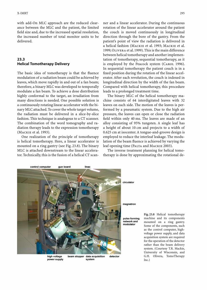
X-IMRT 295

with add-On MLC approach are the reduced clear-ance between the MLC and the patient, the limited fi eld size and, due to the increased spatial resolution, the increased number of total monitor units to be delivered.

23.3 Helical Tomotherapy Delivery

The basic idea of tomotherapy is that the fl uence modulation of a radiation beam could be achieved by leaves, which move rapidly in and out of a fan beam; therefore, a binary MLC was developed to temporally modulate a fan beam. To achieve a dose distribution highly conformal to the target, an irradiation from many directions is needed. One possible solution is a continuously rotating linear accelerator with the bi-nary MLC attached. To cover the whole target volume, the radiation must be delivered in a slice-by-slice fashion. This technique is analogous to a CT scanner. The combination of the word tomography and ra-diation therapy leads to the expression tomotherapy (Mackie et al. 1993).

One realization of the principle of tomotherapy is helical tomotherapy. Here, a linear accelerator is mounted on a ring gantry (see Fig. 23.8). The binary MLC is attached downstream to the linear accelera-tor. Technically, this is the fusion of a helical CT scan-

ner and a linear accelerator. During the continuous rotation of the linear accelerator around the patient the couch is moved continuously in longitudinal direction through the bore of the gantry. From the patient’s point of view the radiation is delivered in a helical fashion (Mackie et al. 1993; Mackie et al. 1999; Olivera et al. 1999). This is the main difference between helical tomotherapy and another implemen-tation of tomotherapy, sequential tomotherapy, as it is employed by the Peacock system (Carol 1996). In sequential tomotherapy the patient couch is in a fi xed position during the rotation of the linear accel-erator. After each revolution, the couch is indexed in longitudinal direction by the width of the fan beam. Compared with helical tomotherapy, this procedure leads to a prolonged treatment time.

The binary MLC of the helical tomotherapy ma-chine consists of 64 interdigitated leaves with 32 leaves on each side. The motion of the leaves is per-formed by a pneumatic system. Due to the high air pressure, the leaves can open or close the radiation fi eld within only 40 ms. The leaves are made of an alloy consisting of 95% tungsten. A single leaf has a height of about 10 cm and projects to a width of 0.625 cm at isocenter. A tongue-and-groove design is employed to reduce the interleaf leakage. The modu-lation of the beam fl uence is achieved by varying the leaf opening time (Palta and Mackie 2003).

The inverse treatment planning for helical tomo-therapy is done by approximating the rotational de-

Fig. 23.8 Helical tomotherapy machine and its components mounted on a ring gantry. Some of the components, such as the control computer, high-voltage power supply, and data acquisition system are required for the operation of the detector rather than the beam delivery system. (Courtesy T.R. Mackie, University of Wisconsin, and G.H. Olivera, TomoTherapy Inc.)

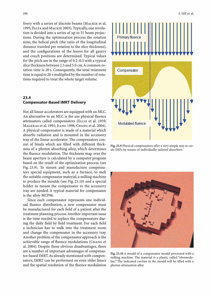
296 S. Nill et al.

livery with a series of discrete beams (Mackie et al. 1995; Palta and Mackie 2003). Typically, one revolu-tion is divided into a series of up to 51 beam projec-tions. During the optimization process the rotation time, the helical pitch (the ratio of the longitudinal distance traveled per rotation to the slice thickness), and the confi gurations of the leaves for all gantry and couch positions are determined. Typical values for the pitch are in the range of 0.2–0.5 with a typical slice thickness between 2.5 and 5.0 cm. A common ro-tation time is 20 s. Consequently, the total treatment time is equal to 20 s multiplied by the number of rota-tions required to treat the whole target volume.

23.4 Compensator-Based IMRT Delivery

Not all linear accelerators are equipped with an MLC. An alternative to an MLC is the use physical fl uence attenuators called compensators (Ellis et al. 1959; Mageras et al. 1991; Jiang 1998; Chang et al. 2004). A physical compensator is made of a material which absorbs radiation and is mounted in the accessory tray of the linear accelerator. The compensators con-sist of bixels which are fi lled with different thick-ness of a photon absorbing alloy, which determines the fl uence modulation. The thickness map over the beam aperture is calculated by a computer program based on the result of the optimization process (see Fig. 23.9). To mount and manufacture compensa-tors special equipment, such as a furnace, to melt the suitable compensator material, a milling machine to produce the moulds (see Fig. 23.10) and a special holder to mount the compensator to the accessory tray are needed. A typical material for compensator is the alloy MCP96.

Since each compensator represents one individ-ual fl uence distribution, a new compensator must be manufactured for each fi eld of a patient after the treatment planning process. Another important issue is the time needed to replace the compensators dur-ing the daily fi eld by fi eld treatment. For each fi eld a technician has to walk into the treatment room and change the compensator in the accessory tray. Another problem of the compensator approach is the achievable range of fl uence modulations (Chang et al. 2004). Despite these obvious disadvantages, there are a number of important advantages of compensa-tor-based IMRT. As already mentioned with compen-sators, IMRT can be performed on even older linacs and the spatial resolution of the fl uence modulation

Fig. 23.9 Physical compensators offer a very simple way to cre-ate IMFs by means of individually tailored absorbers

Fig. 23.10 A mould of a compensator mould processed with a milling machine. The material is a plastic called “obomodu-lan.” The indicated cavities in the mould will be fi lled with a photon attenuation alloy

X-IMRT 297

can be very high, e.g., <5 mm. Another important advantage of compensators is that the total moni-tor units delivered for a complete IMRT plan is only slightly increased compared with the monitor units used for the delivery of a conventional treatment plan. This might be an important fact in the ongo-ing discussion about secondary radiation-induced tumors due to the higher exposure of normal tissue with low doses for MLC-based IMRT delivery (Hall and Wuu 2003).

In conclusion, IMRT with compensators is feasible, but the effort to produce compensators can be very high and special equipment is needed; however, there seems to be advantages which can justify the applica-tion of compensators (Chang 2004).

References

Biggs P, Capalucci J, Russell M (1991) Comparison of the pen-umbra between focused and nondivergent blocks: implica-tions for multileaf collimators. Med Phys 18:753–758

Boesecke R, Becker G, Alandt K, Pastyr O, Doll J, Sclegel W, Lorenz WJ (1991) Modifi cation of a three-dimensional treatment planning system for the use of multileaf colli-mators in conformation readiotherapy. Radiother Oncol 21:261–268

Bortfeld T, Boyer AL, Schlegel W, Kahler DL, Waldron TJ (1994) Realization and verifi cation of three-dimensional confor-mal radiotherapy with modulated fi elds. Int J Radiat Oncol Biol Phys 30:899–908

Bortfeld T, Oelfke U, Nill S (2000) What is the optimum leaf width of a multifl eaf collimator? Med Phys 27:2494–2502

Boyer Al, Yu CX (1999) Intensity-modulated radiation therapy with dynamic multileaf collimators. Semin Radiat Oncol 9:48–59

Carol M, Grant WH III, Pavord D, Eddy P, Targovnik HS, Butler B, Woo S, Figura J, Onufrey V, Grossman R, Selkar R (1996) Initial clinical experience with the Peacock intensity modulation of a 3-D conformal radiation therapy system. Stereotact Funct Neurosurg 66:30–34

Chang SX, Cullip TJ, Deschesne KM, Miller EP, Rosenman JG (2004) Compensators: an alternative IMRT delivery tech-nique. J Appl Clin Med Phys 5:15–36

Convery DI, Webb S (1998) Generation of discrete beam-intensity modulation by dynamic multileaf collimation under minimum leaf separation constraints. Phys Med Biol 43:2521–2538

Cosgrove V, Jahn U, Pfaender M, Bauer S, Budach V, Wurm R (1999) Commissioning of a micro multi-leaf collimator and planning system for stereotactic radiosurgery. Radiother Oncol 50:325–336

Chui CS, Chanf MF, Yorke E, Spirou S, Ling CC (2001) Delivery of intensity-modulated radiation therapy with a conven-tional multileaf collimator: comparison of dynamic and segmental methods. Med Phys 28:2441–2449

Eisbruch A, Kim HM, Terrell JE, Marsh LH, Dawson LA, Ship JA (2001) Xerostomia and its predictors following parotid-

sparing irradiation of head-and-neck cancer. Int J Radiat Oncol Biol Phys 50:695–704

Ellis F, Hall EJ, Oliver R (1959) A compensator for variations in tissue thickness for high energy beams. Br J Radiol 32:421–422

Fiveash JB, Murshed H, Duan J, Hyatt M, Caranto J, Bonner JA, Popple RA (2002) Effect of multileaf collimator leaf width on physical dose distributions in the treatment of CNS and head and neck neoplasms with intensity modulated radia-tion therapy. Med Phys 29:1116–1119

Hall EJ, Wuu CS (2003) Radiation-induced second cancers: the impact of 3D-CRT and IMRT. Int J Radiat Oncol Biol Phys 56:83–88

Hartmann GH, Föhlisch F (2002) Dosimetric characterization of a new miniature multileaf collimator. Phys Med Biol 47:N171–N177

Hug MS, Das IJ, Steinberg T, Galvin JM (2002) A dosimetric comparison of various multileaf collimators. Phys Med Biol 47:N159–N170

Jiang SB (1998) On modulator design for photon beam inten-sity-modulated conformal therapy. Med Phys 25:668–675

Jordan TF, Williams PC (1994) The design and performance characteristics of a multileaf collimator. Phys Med Biol 39:231–251

Kamath S, Sahni S, Ranka S, Li J, Palta J (2004) Comparison of step-and-shoot leaf sequencing algorithms that eliminate tongue-and-groove effect. Phys Med Biol 49:3137–3143

Lee N, Xia P, Quivey JM, Sultanem K, Poon I, Akazawa C, Aka-zawa P, Weinberg , Fu KK (2002) Intensity modulated radio-therapy in the treatment of nasopharyngeal carcinoma: an update of the UCSF experience. Int J Radiat Oncol Biol Phys 53:12–22

LoSasso T, Chui CS, Ling CC (1998) Physical and dosimet-ric aspects of a multileaf collimation system used in the dynamic mode for implementing intensity modulated radiotherapy. Med Phys 25:1919–1927

Ma A, Boyer AL, Xing L, Ma CM (1998) An optimized leaf-set-ting algorithm for beam intensity modulation sung dynamic multileaf collimator. Phys Med Biol 43:1629–1643

Ma L, Boyer A, Ma CM, Xing L (1999) Synchronizing dynamic multileaf collimators for producing two-dimensional intensity-modulated fi elds with minimum beam delivery time. Int J Radiat Oncol Biol Phys 44:1147–1154

Mackie TR, Holmes T, Swerdloff S, Reckwerdt P, Deasy JO, Yang J, Paliwal B, Kinsella T (1993) Tomotherapy: a new concept for the delivery of conformal radiotherapy using dynamic collimation. Med Phys 20:1709–1719

Mackie TR, Holmes TW, Reckwerdt PJ, Yang J (1995) Tomo-therapy: optimized planning and delivery of radiation therapy. Int J Imaging Syst Tech 6:43–55

Mackie TR, Balog J, Ruchala K, Shepard D, Aldridge S, Fitchard E, Reckwerdt PJ, Olivera G, McNutt TR, Metha M (1999) Tomotherapy. Semin Radiat Oncol 9:108–117

Mageras GS, Mohan R, Burman C, Barset GD, Kutcher GJ (1991) Compensators for three dimensional treatment planning. Med Phys 18:133–140

Meeks S, Bova F, Kim S, Tome W, Buatti J, Friedman W (1999) Dosimetric characteristics of a double-focused miniature multileaf collimator. Med Phys 26:729–733

Münter MW, Debus J, Hof H, Nill S, Haring P, Bortfeld T, Wan-nenmacher M (2002) Inverse treatment planning and ste-reotactic intensity-modulated radiation therapy (IMRT) of the tumor and lymph node levels for nasopharyngeal

298 S. Nill et al.

carcinomas. Description of treatment technique, plan com-parison, and case study. Strahlenther Onkol 178:517–523

Nill S, Tücking T, Münter MW, Oelfke U (2005) Intensity modu-lated radiation therapy with multi leaf collimators of differ-ent leaf widths: a comparison of achievable dose distribu-tions. Radiol Oncol75:106–111

Olivera GH, Shepard DM, Ruchala K, Aldridge JS, Kapatoes JM, Fitchard EE, Reckwerdt PJ, Fang G, Balog J, Zachman J and Mackie TR (1999) Tomotherapy. In: Van Dyk J (ed) Modern technology of radiation oncology. Medical Physics Publishing, Madison, Wisconsin

Palta J, Mackie TR (2003) (eds) Medical physics monograph 29:51–75

Siochi A (1999) Minimizing static intensity modulation deliv-ery time using an intensity solid paradigm. Int J Radiat Oncol Biol Phys 43:671–680

Spirou S, Chui C (1994) Generation of arbitrary intensity pro-fi les by dynamic jaws or multileaf collimators. Med Phys 21:1031–1041

Stein J, Bortfeld T, Dorschel B, Schlegel W (1994) Dynamic X-ray compensation for conformal radiotherapy by means of multileaf collimator. Radiother Oncol 32:163–173

Thilmann C, Schulz-Ertner D, Zabel A, Herfarth KK, Wan-nenmacher M, Debus J (2002) Intensity-modulated radio-therapy of sacral chordoma: a case report and a compari-son with stereotactic conformal radiotherapy. Acta Oncol 41:395–399

Thilmann C, Sroka-Perez G, Krempien R, Hoess A, Wannenm-acher M, Debus J (2004) Inversely planned intensity mod-

ulated radiotherapy of the breast including the internal mammary chain: a plan comparison study. Technol Cancer Res Treat 3:69–75

Van Stanvoort J, Heijmen B (1996) Dynamic multileaf collima-tion without tongue-and-groove underdose effects. Phys Med Biol 41:2091–2105

Webb S (1997) The physics of conformal radiotherapy. Advances in technology. Institute of Physics Publishing, Bristol

Webb S (2001) Intensity-modulated radiation therapy. Insti-tute of Physics, Publishing, Bristol

Webb S, Bortfeld T, Stein J, Convery D (1996) The effect of stair-step leaf transmission on the “tongue-and-groove problem” in dynamic radiotherapy with multileaf collima-tor. Phys Med Biol 42, 595–202

Xia P, Verhey LJ (1998) Multileaf collimator leaf sequencing algorithm for intensity modulated beams with multiple static segments. Med Phys 25:1424–1434

Xia P, Geis P, Xing L (1999) Physical characteristics of a min-iature multileaf collimator. Med Phys 26:65–70

Zelefsky M, Fuks Z, Hunt M, Yamada Y, Marion C, Ling C, Amalos H Venkatramen ES, Leibel SA (2002) High-dose intensity modulated radiation therapy for prostate cancer: early toxicity and biochemical outcome in 772 patients. Int J Radiat Oncol Biol Phys 53:1111–1116

Zygmanski P, Kung JH, Jiang SB, Chin L (2003) Dependence of fl uence errors in dynamic IMRT on leaf-positional errors varying with time and leaf number. Med Phys 30:2736–2349

Control of Breathing Motion: Techniques and Models (Gated Radiotherapy) 299

24 Control of Breathing Motion: Techniques and Models (Gated Radiotherapy)

Timothy D. Solberg, N.M. Wink, S.E. Tenn, S. Kriminski, G.D. Hugo, and N. Agazaryan

T. D. Solberg, PhDDepartment of Radiation Oncology, University of Nebraska Medical Center, 987521 Nebraska Medical Center, Omaha, NE 68198-7521, USAT. D. Solberg, PhD; N. M. Wink, MS; S. E. Tenn, MS; S. Kriminski, PhD; N. Agazaryan, PhDDepartment of Radiation Oncology, Suite B265, David Geffen School of Medicine at UCLA, 200 UCLA Medical Plaza, Los Angeles, CA 90096-6951, USAG.D. Hugo, PhDDepartment of Radiation Oncology, William Beaumont Hospital, 3601 W. Thirteen Mile Road, Royal Oak, MI 48073, USA

This work was supported in part by grant # 03-028-01-CCE from the American Cancer Society

24.1 Introduction

It is well known throughout the cancer community that a high degree of tumor control and ultimately cure can be achieved through the administration of appropriate doses of ionizing radiation. Throughout the traditional radiotherapy experience, however, administration of a lethal tumor dose has routinely been limited by the tolerance of nearby healthy tis-sues that cannot be adequately excluded from the radiation fi eld. New methodologies for radiation delivery, such as intensity-modulated radiotherapy (IMRT) and body radiosurgery, offer the possibil-ity for further dose escalation in order to optimally avoid critical structures and reduce treatment-asso-ciated morbidity. With these new delivery techniques, however, the practical and very real problems associ-ated with patient positioning, target localization, and respiratory motion take on added importance. It is disadvantageous and perhaps counterproductive to deliver a very exacting dose distribution when there is uncertainty in the location of the anatomical struc-tures of interest. The IMRT Collaborative Working Group (2001), sponsored by the NCI, recognizes the hazards involved in applying a highly focused radio-therapy approach to moving targets: “application of IMRT to sites that are susceptible to breathing mo-tion should be limited until proper accommodation of motion uncertainties is included.” Thus, for con-tinued clinical gains in the practice of radiotherapy, management of breathing motion is essential.

24.2 Clinical Rationale for Management of Respiratory Motion

Recent clinical gains in a number of tumor sites have been truly remarkable. In prostate cancer, for exam-ple, 5-year survival has increased from 43% for the 5-year period ended in 1954 to 99% for the 5-year

CONTENTS

24.1 Introduction 29924.2 Clinical Rationale for Management of Respiratory Motion 29924.3 Monitoring of Respiratory Motion: Surrogates for Organ Motion 30124.3.1 Monitoring of Respiratory Air fl ow 30124.3.2 Mechanical Monitoring 30224.3.3 Monitoring Using External Markers and Surface Queues 30224.4 Monitoring of Respiratory Motion: Direct Detection of Organ Motion and Correction for Imaging Artifacts 30324.4.1 X-ray and Fluoroscopy 30324.4.2 Computed Tomography 30524.5 Treatment Options to Compensate for Respiratory Motion 30624.5.1 Planning Techniques and Use of Beam Margins 30624.5.2 Abdominal Compression 30724.5.3 Breath-Hold Gating Techniques 30724.5.4 Free-Breathing Gating Techniques 30824.5.5 Tumor Tracking 31024.6 Dosimetric Consequences of Respiratory Motion 31224.7 Conclusion 315 References 315

300 T. D. Solberg et al.

period ended in 2000 (Ries et al. 2004). Gains in breast and head and neck cancers have been equally signifi cant. Radiotherapy has played a central part in these clinical achievements, with clear roles as both a primary and an adjuvant therapy. There remain a number of cancers for which local control and cure remain somewhat elusive, however. Notably, the 5-year survival for lung and primary liver cancers re-mains below 20% (Ries et al. 2004).

Nevertheless, there is increasing evidence in the scientifi c literature to justify the claim that present rates of tumor control and cure for both lung and liver tumors could be improved with judicious use of dose escalation. Morita et al. (1997) analyzed 149 patients with stage-I, medically inoperable non-small cell lung cancer (NSCLC) treated with curative radiotherapy. They observed 3- and 5-year actu-arial survival rates of 34.2 and 22.2%, respectively. Perhaps more importantly, of the patients who died within 5 years, 57% succumbed to local disease. The authors concluded that while “medically inoperable NSCLC patients in stage I should be offered curative radiation therapy, development of some new steps to increase the complete response (CR) rate and local control rate is urgently needed.”

Several techniques have been proposed in an ef-fort to increase control rates and reduce complica-tion rates in irradiation of lung tumors. Robertson et al. (1997a) used CT-based 3D radiation treatment planning in a lung tumor dose escalation study. A total of 48 patients were treated with doses ranging from 69.3 to 92.4 Gy. None of the patients available for evaluation beyond 6 months experienced pneu-monitis, though follow-up times were too short to make conclusive statements regarding local control or survival; however, 30% of the patients receiving 84 Gy or greater had biopsy-proven residual dis-ease. A subsequent analysis reported by Martel et al. (1999) showed a signifi cant improvement in local progression-free survival in patients receiving 70 Gy and above. The authors further stated that the radia-tion dose needed to achieve adequate levels of local control is signifi cantly higher than those historically employed. A number of subsequent clinical investiga-tions have supported the necessity for dose escala-tion in lung cancer (Willner et al. 2002; Roof et al. 2003; Narayan et al. 2004).

Historically, dose escalation has always been ac-companied by increased morbidity. Kwa et al. (1998) investigated pneumonitis rates in 399 patients irra-diated for lung cancer. They observed a clear cor-relation between the mean biological lung dose and the incidence of pneumonitis, suggesting that more

sophisticated delivery techniques are necessary in order to stabilize or reduce complication rates with further dose escalation.

While radiation therapy has traditionally repre-sented the most suitable substitute for surgery for pa-tients with many localized solid tumors, it has played no appreciable role for intrahepatic cancers. The main reason is that hepatic malignancies and normal liver tissue are equally sensitive to radiation (Reed and Cox 1966; Lawrence et al. 1995). Until recently, radiation oncologists could not irradiate the tumor within the liver without damaging the surrounding liver parenchyma; however, precision-oriented ra-diation techniques such as conformal radiotherapy (CRT) and IMRT can create a radiation dose distri-bution that conforms tightly along the 3D irregular contour of the tumor, while simultaneously sparing the normal tissues. Several institutional studies have been published to indicate the effi cacy of such ap-proach for both primary and metastatic liver tumors. Robertson et al. (1997b) presented their experience in treating patients with intrahepatic and bile duct cancers, with concurrent intra-arterial FdUrd infu-sion for radiation sensitization. They showed that overall progression-free survival within the liver was 50% in 2 years and 4-year actuarial survival rate was 20%. No late hepatic toxicity was observed. Other studies have similarly demonstrated that high prob-ability of local tumor control and low likelihood of late normal tissue toxicity can be attainable with these focused radiotherapy techniques (Sato et al. 1998; Blomgren et al. 1999).

The issue of respiratory motion has long been rec-ognized as a major limitation in the management of many radiotherapy patients and there have been nu-merous studies over many years detailing signifi cant motion (of up to several centimeters) of thoracic and abdominal structures with respiration (Ross et al. 1990; Balter et al. 1996; Ekberg et al. 1998; Balter et al. 2001). Even respiratory motion of the prostate has been observed (Kitamura et al. 2002a). These and many other studies are discussed in greater de-tail later in this chapter.

Thus, while recent clinical results do suggest that higher doses may be administered with some de-gree of safety, continuing suboptimal control rates, even at high radiation doses, suggests that further enhancements in the delivery techniques to reduce respiratory motion are needed. Willett et al. (1987) speculated that radiotherapy gated with respiration may be benefi cial in the treatment of Hodgkin’s dis-ease. Suit et al. (1988) called gated radiotherapy an “important means for further improvements in dose

Control of Breathing Motion: Techniques and Models (Gated Radiotherapy) 301

distributions.” In the University of Michigan radio-therapy experience in liver cancer results suggested that “elimination of the margin added to hepatic tar-get volumes for patient ventilation could lead on av-erage to clinically meaningful increases in dose (and TCP) without increasing the predicted frequency of complications” (Ten Haken et al. 1997). In a treat-ment planning study to evaluate the effect of IMRT in lung irradiation, Brugmans et al. (1997) cautioned that, with respiration-induced organ motion of up to several centimeters reported in the literature, “fi eld size reduction for lung tumors, although benefi cial for the surrounding lung tissue, should be applied with great care because of the target motion due to respiration.” Mehta et al. (2001) modeled the lung tumor response data of Martel et al. (1999) and con-cluded that “if higher doses can be delivered to lim-ited volumes using advanced conformal techniques such as IMRT gated for breathing, together with on-line verifi cation and adaptation, large increases of local control would be expected.” Narayan et al. (2004) echoed these sentiments: “further dose esca-lation can also be accomplished using techniques to reduce the volume of normal lung irradiated.” Clearly then, continued improvement in clinical outcomes through dose escalation will increasingly be limited by the practical and very real problems associated with respiratory motion.

24.3 Monitoring of Respiratory Motion: Surrogates for Organ Motion

A variety of methodologies have been employed to monitor human respiratory motion. These can be grouped into two general categories: those which directly monitor the motion of a tumor and/or criti-cal anatomy, typically through an imaging procedure such as fl uoroscopy, and those which monitor a sur-rogate for target movement. A number of disparate technologies have been investigated as surrogates for target motion, including the monitoring of re-spiratory air fl ow, mechanical devices which record variations in surface tension, and camera-based sys-tems which monitor the motion of passive and active markers positioned on a patient’s skin. In this section, we summarize the operation and experience of these surrogate methodologies.

24.3.1 Monitoring of Respiratory Air fl ow

Devices for monitoring respiratory air fl ow can be divided into two general categories: those which measure temperature as a surrogate of fl ow, includ-ing thermistors and thermocouples, and those which directly monitor air fl ow, such as a nasal cannula or spirometer. A thermistor is a ceramic semiconductor which changes its electrical resistance as a function of temperature. Thermistors belong to a class of de-tectors generally referred to as resistive temperature devices (RTDs) which require the application of a current in order to measure the resistance changes. Thermistors are extremely sensitive, exhibiting a large change in resistance with small changes in tem-perature. In contrast, a thermocouple consists of two different metallic alloys across which an electromo-tive force (emf) is induced when the alloys differ in temperature. The voltage change in a thermocouple is approximately linear with the change in temperature, and therefore thermocouples are much less sensi-tive than thermistors. Both thermistors and thermo-couples have response times well below 1 s, and both have been used routinely in monitoring respiratory fl ow for a variety of applications (Xiong et al. 1993; Marks et al. 1995; Norman et al. 1997; Farre et al. 1998; Lindemann et al. 2002). Kubo et al. (1996) concluded that both thermistors and thermocouples provided adequate signal characteristics for respi-ration-gated radiotherapy techniques. Marks et al. (1995) also concluded that thermocouples accurately reproduced respiratory rates, while several authors have pointed out shortcomings with both types of devices (Xiong et al. 1993; Norman et al. 1997; Farre et al. 1998; Lindemann et al. 2002). In practice, both thermistors and thermocouples and designed to be placed just below the nostrils.

Spirometry is a catch-all term for technologies that provide a direct measurement of volume displace-ment or air fl ow. Volume displacement can be mea-sured using a piston or bellows, although such an ap-proach is more diffi cult to quantify and is somewhat impractical; therefore, spirometers that utilize sen-sors to measure fl ow have largely replaced volume-displacement systems. Furthermore, fl ow-sensing spirometers can also monitor volume using digital integration techniques. The most common fl ow-sens-ing spirometric sensor is the pneumotachometer, a small tube with an inherent resistance to fl ow. By monitoring the pressure drop across the resistance, fl ow can be determined. Open-loop spirometry, such as that performed using a mask or nasal cannula, al-

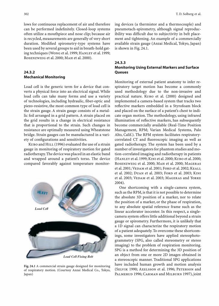
302 T. D. Solberg et al.

lows for continuous replacement of air and therefore can be performed indefi nitely. Closed-loop systems often utilize a mouthpiece and nose clip; because air is recycled, measurements are generally of very short duration. Modifi ed spirometry-type systems have been used by several groups to aid in breath-hold gat-ing techniques (Wong et al. 1999; Hanley et al. 1999; Rosenzweig et al. 2000; Mah et al. 2000).

24.3.2 Mechanical Monitoring

Load cell is the generic term for a device that con-verts a physical force into an electrical signal. While load cells can take many forms and use a variety of technologies, including hydraulic, fi ber-optic and piezo-resistive, the most common type of load cell is the strain gauge. A strain gauge consists of a metal-lic foil arranged in a grid pattern. A strain placed on the grid results in a change in electrical resistance that is proportional to the strain. Such changes in resistance are optimally measured using Wheatstone bridge. Strain gauges can be manufactured in a vari-ety of confi gurations and sensitivities.

Kubo and Hill (1996) evaluated the use of a strain gauge in monitoring of respiratory motion for gated radiotherapy. The device was placed in an elastic band and wrapped around a patient’s torso. The device compared favorably against temperature monitor-

ing devices (a thermistor and a thermocouple) and pneumotach-spirometry, although signal reproduc-ibility was diffi cult due to subjectivity in belt place-ment and tightening. An example of a commercially available strain gauge (Anzai Medical, Tokyo, Japan) is shown in Fig. 24.1.

24.3.3 Monitoring Using External Markers and Surface Queues

Monitoring of external patient anatomy to infer re-spiratory target motion has become a commonly used methodology due to the non-invasive and practical nature. Kubo et al. (2000) designed and implemented a camera-based system that tracks two refl ective markers embedded in a Styrofoam block and placed on the surface of a patient’s chest to indi-cate organ motion. The methodology, using infrared illumination of refl ective markers, has subsequently become commercially available (Real-Time Position Management, RPM; Varian Medical Systems, Palo Alto, Calif.). The RPM system facilitates respiratory-correlated CT and fl uoroscopic imaging as well as gated radiotherapy. The system has been used by a number of investigators for phantom studies and mo-tion-correlated imaging and radiotherapy in patients (Hanley et al. 1999; Kini et al. 2000; Kubo et al. 2000; Rosenzweig et al. 2000; Mah et al. 2000; Mageras et al. 2001; Vedam et al. 2001; Ford et al. 2002; Keall et al. 2002; Duan et al. 2003; Ford et al. 2003; Kini et al. 2003; Vedam et al. 2003; Mageras and Yorke 2004).

One shortcoming with a single-camera system, such as the RPM, is that it is not possible to determine the absolute 3D position of a marker, nor to relate the position of a marker, or the phase of respiration, to any absolute spatial reference frame such as the linear accelerator isocenter. In this respect, a single-camera system offers little additional beyond a strain gauge or spirometry. Furthermore, it is unlikely that a 1D signal can characterize the respiratory motion of a patient adequately. To overcome these shortcom-ings, some investigators have applied stereophoto-grammetry (SPG, also called stereometry or stereo imaging) to the problem of respiration monitoring. SPG is a method for determining the 3D position of an object from one or more 2D images obtained in a stereoscopic manner. Traditional SPG applications have included human growth and motion analysis (Selvik 1990; Axelsson et al. 1996; Peterson and Palmerud 1996; Carman and Milburn 1997), joint

Fig. 24.1 A commercial strain gauge designed for monitoring of respiratory motion. (Courtesy Anzai Medical Co., Tokyo, Japan)

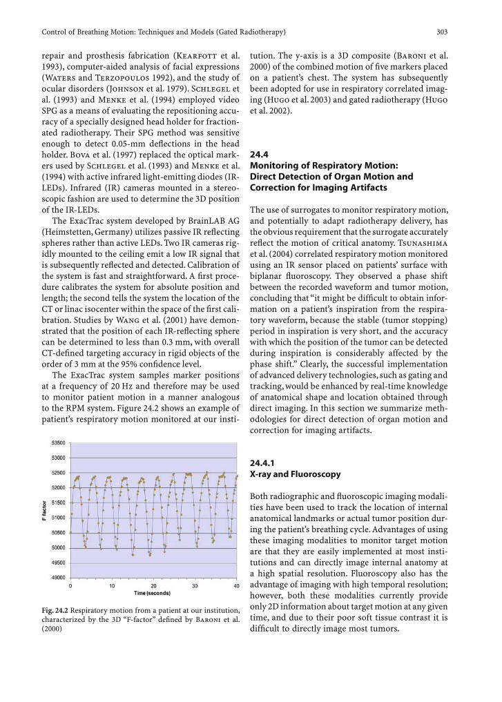
Control of Breathing Motion: Techniques and Models (Gated Radiotherapy) 303

repair and prosthesis fabrication (Kearfott et al. 1993), computer-aided analysis of facial expressions (Waters and Terzopoulos 1992), and the study of ocular disorders (Johnson et al. 1979). Schlegel et al. (1993) and Menke et al. (1994) employed video SPG as a means of evaluating the repositioning accu-racy of a specially designed head holder for fraction-ated radiotherapy. Their SPG method was sensitive enough to detect 0.05-mm defl ections in the head holder. Bova et al. (1997) replaced the optical mark-ers used by Schlegel et al. (1993) and Menke et al. (1994) with active infrared light-emitting diodes (IR-LEDs). Infrared (IR) cameras mounted in a stereo-scopic fashion are used to determine the 3D position of the IR-LEDs.

The ExacTrac system developed by BrainLAB AG (Heimstetten, Germany) utilizes passive IR refl ecting spheres rather than active LEDs. Two IR cameras rig-idly mounted to the ceiling emit a low IR signal that is subsequently refl ected and detected. Calibration of the system is fast and straightforward. A fi rst proce-dure calibrates the system for absolute position and length; the second tells the system the location of the CT or linac isocenter within the space of the fi rst cali-bration. Studies by Wang et al. (2001) have demon-strated that the position of each IR-refl ecting sphere can be determined to less than 0.3 mm, with overall CT-defi ned targeting accuracy in rigid objects of the order of 3 mm at the 95% confi dence level.

The ExacTrac system samples marker positions at a frequency of 20 Hz and therefore may be used to monitor patient motion in a manner analogous to the RPM system. Figure 24.2 shows an example of patient’s respiratory motion monitored at our insti-

tution. The y-axis is a 3D composite (Baroni et al. 2000) of the combined motion of fi ve markers placed on a patient’s chest. The system has subsequently been adopted for use in respiratory correlated imag-ing (Hugo et al. 2003) and gated radiotherapy (Hugo et al. 2002).

24.4 Monitoring of Respiratory Motion: Direct Detection of Organ Motion and Correction for Imaging Artifacts

The use of surrogates to monitor respiratory motion, and potentially to adapt radiotherapy delivery, has the obvious requirement that the surrogate accurately refl ect the motion of critical anatomy. Tsunashima et al. (2004) correlated respiratory motion monitored using an IR sensor placed on patients’ surface with biplanar fl uoroscopy. They observed a phase shift between the recorded waveform and tumor motion, concluding that “it might be diffi cult to obtain infor-mation on a patient’s inspiration from the respira-tory waveform, because the stable (tumor stopping) period in inspiration is very short, and the accuracy with which the position of the tumor can be detected during inspiration is considerably affected by the phase shift.” Clearly, the successful implementation of advanced delivery technologies, such as gating and tracking, would be enhanced by real-time knowledge of anatomical shape and location obtained through direct imaging. In this section we summarize meth-odologies for direct detection of organ motion and correction for imaging artifacts.

24.4.1 X-ray and Fluoroscopy

Both radiographic and fl uoroscopic imaging modali-ties have been used to track the location of internal anatomical landmarks or actual tumor position dur-ing the patient’s breathing cycle. Advantages of using these imaging modalities to monitor target motion are that they are easily implemented at most insti-tutions and can directly image internal anatomy at a high spatial resolution. Fluoroscopy also has the advantage of imaging with high temporal resolution; however, both these modalities currently provide only 2D information about target motion at any given time, and due to their poor soft tissue contrast it is diffi cult to directly image most tumors.

Fig. 24.2 Respiratory motion from a patient at our institution, characterized by the 3D “F-factor” defi ned by Baroni et al. (2000)

304 T. D. Solberg et al.

As noted above, radiographic techniques have lim-ited use in directly detecting organ or tumor motion. The diaphragm boundary, however, is easily detected with these modalities due to the good contrast be-tween lung and upper abdominal structures. It has, therefore, been used as a landmark to track respi-ratory motion and as a surrogate for thoracic tis-sue motion (Mageras et al. 2001; Ford et al. 2002; Wagman et al. 2003; Vedam et al. 2001; Vedam et al. 2003). Fluoroscopy has also been used to track the motion of other visible anatomical targets in the tho-rax or abdomen (Minohara et al. 2000), including the motion of some lung tumors which have enough physical contrast to be observed directly (Chen et al. 2001; Sixel et al. 2001; Sixel et al. 2003).

In order to track targets using these modalities, the patient is typically set up in the treatment posi-tion under a fl uoroscopically capable radiotherapy simulator or custom fl uoroscopic system (Chen et al. 2001; Ruschin and Sixel 2002). The patients may be asked to follow recorded breathing instructions to create a more stable breathing pattern while a short (30–90 s) loop of images is taken (Vedam et al. 2003; Mageras et al. 2001). The acquisition rate using fl uo-roscopy in these studies was generally 10 to 15 frames per second (Vedam et al. 2003; Sixel et al. 2003).

Both radiographic and fl uoroscopic imaging suf-fer from poor soft tissue contrast. Due to this limita-tion radio-opaque fi ducial markers have been used to report soft tissue positions in or near the target. These fi ducial markers are generally 2-mm gold spheres (Shirato et al. 2003) or rods having diam-eters of approximately 1 mm and lengths of 3–4 mm (Ozhasoglu and Murphy 2002; Whyte et al. 2003). The markers have been implanted using large-gauge needles (Kitamura et al. 2003), they have been su-tured into place during surgery (Ozhasoglu et al. 2002), and they have been placed via bronchial endoscopy for those locations accessible via this approach (Seppenwoolde et al. 2002). The mark-ers have been placed into or near tumors including those of the lung (Shirato et al. 2000a; Shimizu et al. 2001; Seppenwoolde et al. 2002; Ozhasoglu et al. 2002; Whyte et al. 2003, Shirato et al. 2003), liver (Shirato et al. 2000a; Kitamura et al. 2003; Kitamura et al. 2002c, Shirato et al. 2003), pancreas (Schweikard et al. 2000, Ozhasoglu et al. 2002), prostate (Kitamura et al. 2002b, Shirato et al. 2003; Kitamura et al. 2002c) as well as the bladder and rectum (Shirato et al. 2000a).

Because the metal markers are surrogates for the targets in which they are implanted, it is important that they remain fi xed relative to their target of in-

terest. Kitamura et al. (2002c) and Shirato et al. (2003) have addressed this concern as it relates to implantation of 2-mm gold spheres into prostate, liver, and lung tumors. In their study, Kitamura et al. (2002c) estimated the migration of a single gold fi ducial to be no greater than 0.3, 2.5, and 1.9 mm in the liver, and within 1.0, 1.2, and 2.0 mm in the prostate for the left–right, cranial–caudal, and ante-rior–superior directions, respectively. Using a three marker method in their study, Shirato et al. (2003) found that the center of mass of the three markers remain in relatively fi xed positions when inserted into prostate, liver, or when wedged into regions of the bronchial tree having diameter less than that of the marker; however, the markers did not remain se-curely fi xed when inserted directly into centrally lo-cated lung tumors which necessitated dropping of at least one marker from the original implant location occurred in all three centrally located lung tumors studied. Ozhasoglu et al. (2002) sutured spherical gold fi ducials into the pancreas of one patient dur-ing exploratory laparoscopic surgery; it was expected that these markers remained fi xed in this organ.

It is also important that the internally placed fi du-cial markers be easily discernible in the radiographic or fl uoroscopic images. The real-time tumor-track-ing system described by Shirato et al. (2000b) uses an automatic template matching algorithm to locate the fi ducial markers in the images. Using this sys-tem to track and treat 20 lung tumors, Shimizu et al. (2001) found occasions when the 2-mm markers were diffi cult to visualize due to patient thickness. The ExacTracGating system (BrainLAB AG, Heimstetten, Germany) was installed recently at our institution. Like other fl uoroscopic systems, it uses two X-ray sources, with central-beam axes crossing at the linac isocenter, incident on opposing fl at panels. We have observed that 2-mm lead BBs placed into an IMRT phantom (CIRS, Norfolk, Va.) are easily visualized.

Excess skin dose due to fl uoroscopy is a concern while tracking the internal fi ducial markers. This is especially true if the fl uoroscopic X-rays will be run continuously during treatment. Using TLDs in a phan-tom study of the real-time tumor-tracking radiother-apy system, Shirato et al. (2000b) measured the en-trance dose rate for two settings on their fl uoroscopy units. For a 70-kV setting with a 2-ms pulse width they measured an entrance dose rate of 1.76 mGy/min while a 120-kV setting with a 4-ms pulse width gave an entrance dose rate of 10.74 mGy/min. They estimate that the excess dose to the skin from track-ing the target with fl uoroscopy may correspond to as much as 1% of the total prescribed dose. In a study

Control of Breathing Motion: Techniques and Models (Gated Radiotherapy) 305

using a Varian Ximatron C-Series Simulator in fl uo-roscopy mode, Chen et al. (2001) measured larger surface dose rates of 1.25–9.82 cGy/min while using a setting of 65 kVp and 3 mA.

24.4.2 Computed Tomography

Detection of organ motion under respiration and correction for imaging artifacts produced by this mo-tion can be accomplished in various manners. One of the easiest and most direct ways to correct for mo-tion artifacts is to have the patient hold their breath during scanning, if they are able. Various groups have experimented with voluntary breath-hold techniques at inhale and exhale during deep breathing (Aruga et al. 2000; Balter et al. 1998; Giraud et al. 2001). This technique, however, prevents images from being ob-tained at the mean tumor position, which could pro-duce potential problems if breathing is not accounted for during treatment. Also, deep breathing leads to larger displacements in target location than would occur during normal breathing. The use of an active breathing control (ABC) device has been investigated to help account for these problems (Wong et al. 1997, 1999). With the ABC device, a valve is closed on the device to stop the breathing cycle at a specifi c phase. This technique allows for imaging at any position in the cycle; however, there is some concern that organ motion during breathing under the restraint of this device is different from that during free breathing.

Another straightforward approach towards ob-taining a CT representation of tumor motion is slow CT scanning (De Koste et al. 2001; De Koste et al. 2003; Lagerwaard et al. 2001). In this technique, scanning is performed at a much slower rate than nor-mal, resulting in full tumor motion during each slice acquisition. The extent of tumor motion can then be visualized under normal breathing so long as there is suffi cient tumor contrast from background. The mean tumor location can also be inferred from the points of highest intensity on the temporally blurred slice. The drawback to this technique, however, is that the exact tumor shape and size are unknown.

Prospective respiratory-gated CT provides a complete image set at one phase of respiration with slightly more effort than the aforementioned tech-niques (Ritchie et al. 1994). In this approach, nor-mal respiration is monitored with some surrogate for organ motion (see section 24.3). The CT scanner is then triggered to acquire axial slices every time the desired phase of respiration is achieved. This phase

must be chosen a priori and is normally chosen to be end inhale or exhale since the least tumor motion is assumed to be traversed in these phases. Multiple scans are required if multiple phases are desired, which increases both scan time and dose.

Retrospective respiratory gated CT offers the most information about the organ of interest under motion with the highest workload. In this context, it is often referred to as respiratory-correlated CT (RCCT) or 4D CT, the fourth dimension being time. Two of the most extensively studied approaches both utilize an external surrogate for organ motion to monitor res-piration throughout the scan, but they differ in their image acquisition step. Some groups acquire images under a low-pitch helical scan, ensuring enough overlap for a suffi cient amount of data (Ford et al. 2003; Keall et al. 2004; Vedam et al. 2003). Data loss, causing gaps in image sets, may occur if the detector row(s) pass the object of interest before one respira-tion cycle plus one fan angle is complete. This prob-lem lessens with the use of low-pitch multislice scan-ners. Other groups have investigated what is referred to as an axial cine approach (Low et al. 2003a, b; Pan et al. 2004; Rietzel et al. 2003; Wahab et al. 2003). In this technique, several axial slices are acquired at one couch position. The scanner is then stopped and translated to the next position and the process is re-peated.

In both of these techniques, a direct connection between the scanner and the motion sensor is estab-lished so that the exact time of image acquisition can be recorded. This allows all of the image data to have a corresponding phase of respiration associated with it (Fig. 24.3). If the phase of respiration is known, then all of the data in one phase can be grouped to-gether for a complete image set with less temporal blur. Reconstruction of the data can be performed either before or after the phase grouping.

Both of these techniques allow for the exact tu-mor trajectory to be known since image sets can be obtained for every phase. A limitation to these tech-niques is the need for a relatively regular motion for proper binning. Breathing training techniques can help reduce irregularities in the breathing cycle (Allen et al. 2004; Kini et al. 2003); however, some irregular breathing artifacts may still occur.

Prior to the RCCT approaches described, various other retrospective techniques have been proposed to correct for motion-induced artifacts on other imag-ing systems. For example, Lu and Mackie (2002) pre-sented a motion correction algorithm implemented in sinogram space for tomotherapy. Dhanantwari et al. (2001a, b) presented various mathematical tech-

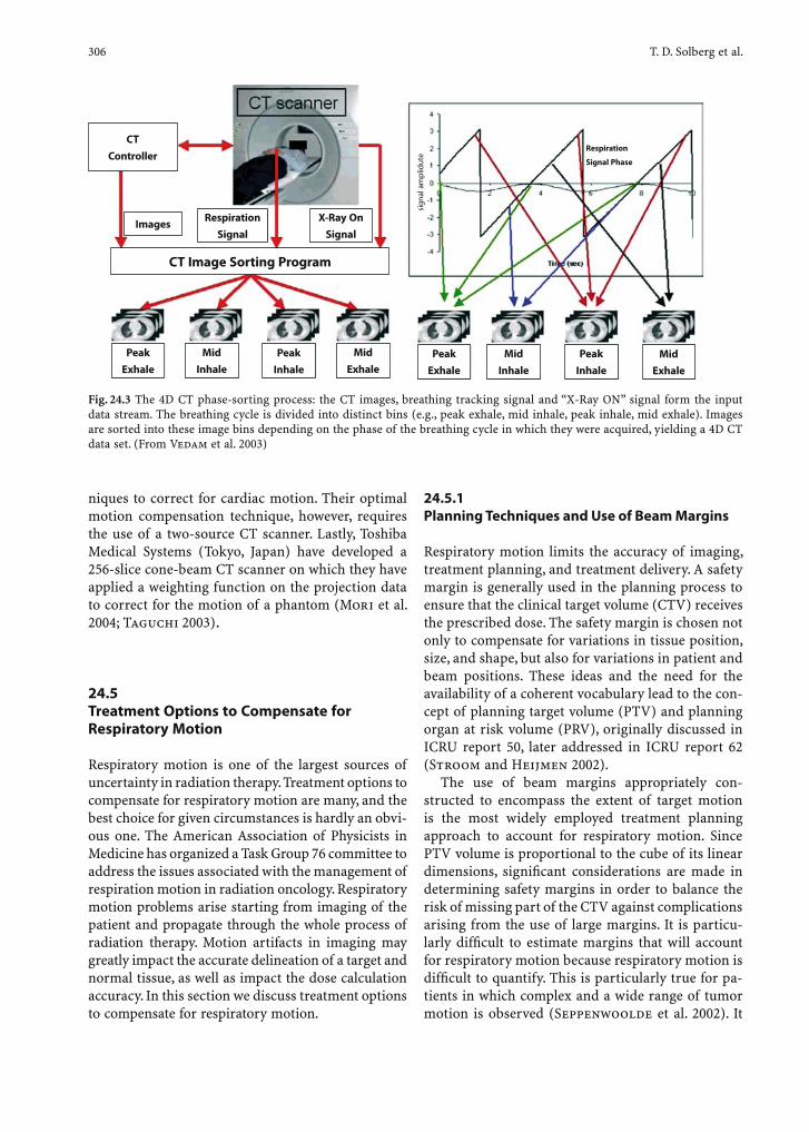
306 T. D. Solberg et al.

niques to correct for cardiac motion. Their optimal motion compensation technique, however, requires the use of a two-source CT scanner. Lastly, Toshiba Medical Systems (Tokyo, Japan) have developed a 256-slice cone-beam CT scanner on which they have applied a weighting function on the projection data to correct for the motion of a phantom (Mori et al. 2004; Taguchi 2003).

24.5 Treatment Options to Compensate for Respiratory Motion

Respiratory motion is one of the largest sources of uncertainty in radiation therapy. Treatment options to compensate for respiratory motion are many, and the best choice for given circumstances is hardly an obvi-ous one. The American Association of Physicists in Medicine has organized a Task Group 76 committee to address the issues associated with the management of respiration motion in radiation oncology. Respiratory motion problems arise starting from imaging of the patient and propagate through the whole process of radiation therapy. Motion artifacts in imaging may greatly impact the accurate delineation of a target and normal tissue, as well as impact the dose calculation accuracy. In this section we discuss treatment options to compensate for respiratory motion.

24.5.1 Planning Techniques and Use of Beam Margins

Respiratory motion limits the accuracy of imaging, treatment planning, and treatment delivery. A safety margin is generally used in the planning process to ensure that the clinical target volume (CTV) receives the prescribed dose. The safety margin is chosen not only to compensate for variations in tissue position, size, and shape, but also for variations in patient and beam positions. These ideas and the need for the availability of a coherent vocabulary lead to the con-cept of planning target volume (PTV) and planning organ at risk volume (PRV), originally discussed in ICRU report 50, later addressed in ICRU report 62 (Stroom and Heijmen 2002).

The use of beam margins appropriately con-structed to encompass the extent of target motion is the most widely employed treatment planning approach to account for respiratory motion. Since PTV volume is proportional to the cube of its linear dimensions, signifi cant considerations are made in determining safety margins in order to balance the risk of missing part of the CTV against complications arising from the use of large margins. It is particu-larly diffi cult to estimate margins that will account for respiratory motion because respiratory motion is diffi cult to quantify. This is particularly true for pa-tients in which complex and a wide range of tumor motion is observed (Seppenwoolde et al. 2002). It

Peak

Exhale

Mid

Inhale

Peak

InhalePeak

Exhale

Mid

ExhaleMid

Inhale

Peak

Inhale

Mid

Exhale

CT

Controller

CT Image Sorting Program

ImagesRespiration

Signal

X-Ray On

Signal

sign

al a

mpl

idut

e

Respiration

Signal Phase

Fig. 24.3 The 4D CT phase-sorting process: the CT images, breathing tracking signal and “X-Ray ON” signal form the input data stream. The breathing cycle is divided into distinct bins (e.g., peak exhale, mid inhale, peak inhale, mid exhale). Images are sorted into these image bins depending on the phase of the breathing cycle in which they were acquired, yielding a 4D CT data set. (From Vedam et al. 2003)

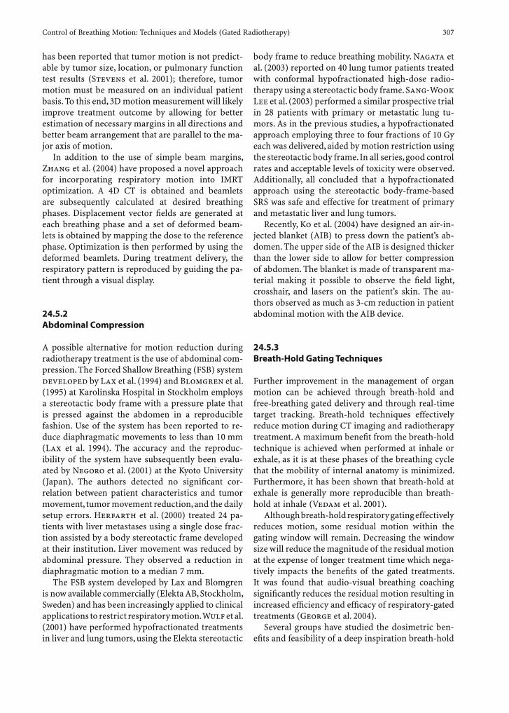
Control of Breathing Motion: Techniques and Models (Gated Radiotherapy) 307

has been reported that tumor motion is not predict-able by tumor size, location, or pulmonary function test results (Stevens et al. 2001); therefore, tumor motion must be measured on an individual patient basis. To this end, 3D motion measurement will likely improve treatment outcome by allowing for better estimation of necessary margins in all directions and better beam arrangement that are parallel to the ma-jor axis of motion.

In addition to the use of simple beam margins, Zhang et al. (2004) have proposed a novel approach for incorporating respiratory motion into IMRT optimization. A 4D CT is obtained and beamlets are subsequently calculated at desired breathing phases. Displacement vector fi elds are generated at each breathing phase and a set of deformed beam-lets is obtained by mapping the dose to the reference phase. Optimization is then performed by using the deformed beamlets. During treatment delivery, the respiratory pattern is reproduced by guiding the pa-tient through a visual display.

24.5.2 Abdominal Compression

A possible alternative for motion reduction during radiotherapy treatment is the use of abdominal com-pression. The Forced Shallow Breathing (FSB) system developed by Lax et al. (1994) and Blomgren et al. (1995) at Karolinska Hospital in Stockholm employs a stereotactic body frame with a pressure plate that is pressed against the abdomen in a reproducible fashion. Use of the system has been reported to re-duce diaphragmatic movements to less than 10 mm (Lax et al. 1994). The accuracy and the reproduc-ibility of the system have subsequently been evalu-ated by Negoro et al. (2001) at the Kyoto University (Japan). The authors detected no signifi cant cor-relation between patient characteristics and tumor movement, tumor movement reduction, and the daily setup errors. Herfarth et al. (2000) treated 24 pa-tients with liver metastases using a single dose frac-tion assisted by a body stereotactic frame developed at their institution. Liver movement was reduced by abdominal pressure. They observed a reduction in diaphragmatic motion to a median 7 mm.

The FSB system developed by Lax and Blomgren is now available commercially (Elekta AB, Stockholm, Sweden) and has been increasingly applied to clinical applications to restrict respiratory motion. Wulf et al. (2001) have performed hypofractionated treatments in liver and lung tumors, using the Elekta stereotactic

body frame to reduce breathing mobility. Nagata et al. (2003) reported on 40 lung tumor patients treated with conformal hypofractionated high-dose radio-therapy using a stereotactic body frame. Sang-Wook Lee et al. (2003) performed a similar prospective trial in 28 patients with primary or metastatic lung tu-mors. As in the previous studies, a hypofractionated approach employing three to four fractions of 10 Gy each was delivered, aided by motion restriction using the stereotactic body frame. In all series, good control rates and acceptable levels of toxicity were observed. Additionally, all concluded that a hypofractionated approach using the stereotactic body-frame-based SRS was safe and effective for treatment of primary and metastatic liver and lung tumors.

Recently, Ko et al. (2004) have designed an air-in-jected blanket (AIB) to press down the patient’s ab-domen. The upper side of the AIB is designed thicker than the lower side to allow for better compression of abdomen. The blanket is made of transparent ma-terial making it possible to observe the fi eld light, crosshair, and lasers on the patient’s skin. The au-thors observed as much as 3-cm reduction in patient abdominal motion with the AIB device.

24.5.3 Breath-Hold Gating Techniques

Further improvement in the management of organ motion can be achieved through breath-hold and free-breathing gated delivery and through real-time target tracking. Breath-hold techniques effectively reduce motion during CT imaging and radiotherapy treatment. A maximum benefi t from the breath-hold technique is achieved when performed at inhale or exhale, as it is at these phases of the breathing cycle that the mobility of internal anatomy is minimized. Furthermore, it has been shown that breath-hold at exhale is generally more reproducible than breath-hold at inhale (Vedam et al. 2001).

Although breath-hold respiratory gating effectively reduces motion, some residual motion within the gating window will remain. Decreasing the window size will reduce the magnitude of the residual motion at the expense of longer treatment time which nega-tively impacts the benefi ts of the gated treatments. It was found that audio-visual breathing coaching signifi cantly reduces the residual motion resulting in increased effi ciency and effi cacy of respiratory-gated treatments (George et al. 2004).

Several groups have studied the dosimetric ben-efi ts and feasibility of a deep inspiration breath-hold

308 T. D. Solberg et al.

(DIBH) technique in the treatment of lung tumors (Hanley et al. 1999; Mah et al. 2000; Rosenzweig et al. 2000). Two main benefi ts of DIBH are the reduc-tion of the lung density and reduction of tumor mo-tion. The DIBH technique involves verbally coaching the patient to the same, reproducible deep inspiration level. Although the DIBH technique appears feasible for clinical implementation, the technique requires comprehensive quality assurance procedures to en-sure accurate treatment delivery.

Active breathing control, fi rst introduced by Wong et al. (1999) at William Beaumont Hospital, repro-ducibly facilitates breath-hold without requiring the patient to reach maximum inspiration capacity (Frazier et al. 2004; Remouchamps et al. 2003a–c; Stromberg et al. 2000). Elekta has since commercial-ized the method under trademark Active Breathing Coordinator. The method has been also imple-mented at Mount Vernon Cancer Centre (Northwood, Middlesex, UK; Wilson et al. 2003). The ABC appara-tus can be used to suspend breathing at any pre-de-termined position along the normal breathing cycle. The system makes use of digital spirometer to mea-sure the respiratory trace. The spirometer actively controls a balloon valve, consequently taking control over the patients breath-hold. In the example shown in Fig. 24.4, the patient was initially brought to quiet tidal breathing and then verbally coached to perform a slow deep inspiration, a slow deep expiration, and a second slow deep inspiration followed by breath-hold. Treatment planning and delivery can then be performed at identical ABC conditions with minimal margin for breathing motion. It is even possible to use the ABC method with standard operation of the accelerator to deliver therapy with a short beam on

time, where tumor and organ positions are immobi-lized before the beam is turned on and not released until the beam is turned off.

24.5.4 Free-Breathing Gating Techniques

Active gating is another available option of exter-nal beam radiotherapy applied to regions affected by intra-fraction motion. Respiratory gating involves the administration of radiation within a particular window of the patient’s breathing cycle as demon-strated in Fig. 24.5. This method requires monitoring patient’s respiratory motion using either an external or internal fi ducial markers. To date, the only com-mercially available respiratory gating systems are the Varian RPM system (described in section 24.3.3) and the BrainLAB ExacTracGating system.

A main obstacle for active gating is the diffi culty associated with real-time detection of the moving target location during treatment. The RPM gating system uses an external IR marker as a surrogate for tumor motion and may not necessarily correlate with internal motion (Tsunashima et al. 2004). In contrast, the ExacTracGating system combines the capability to track externally placed markers in three dimensions with a digital radiography system capa-ble of locating internally placed fi ducials such as gold BBs. While the paradigm is similar to the Cyberknife, the linac does not move dynamically and the imag-ing system does not try to fi nd a tumor trajectory. Instead, the system assumes that the target position is correlated to the position of the surface markers during a given window in the respiratory cycle. This

Fig. 24.4 Representation of spi-rometry tracings from the modi-fi ed slow vital capacity maneuver and the deep inspiration breath-hold. (From Rosenzweig et al. 2000)

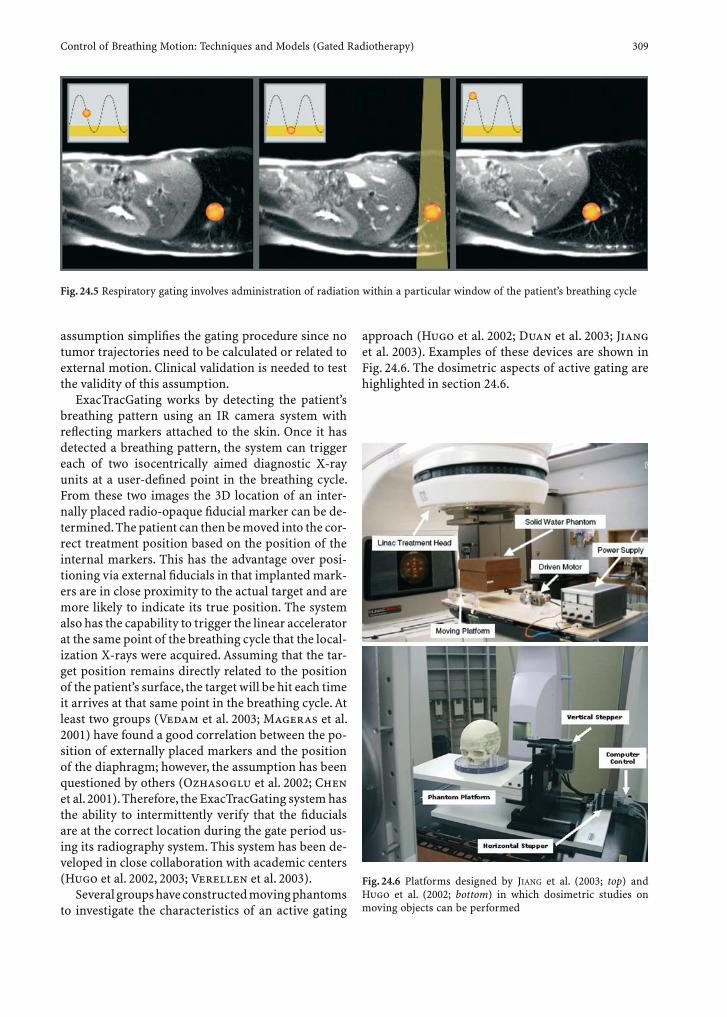
Control of Breathing Motion: Techniques and Models (Gated Radiotherapy) 309

assumption simplifi es the gating procedure since no tumor trajectories need to be calculated or related to external motion. Clinical validation is needed to test the validity of this assumption.

ExacTracGating works by detecting the patient’s breathing pattern using an IR camera system with refl ecting markers attached to the skin. Once it has detected a breathing pattern, the system can trigger each of two isocentrically aimed diagnostic X-ray units at a user-defi ned point in the breathing cycle. From these two images the 3D location of an inter-nally placed radio-opaque fi ducial marker can be de-termined. The patient can then be moved into the cor-rect treatment position based on the position of the internal markers. This has the advantage over posi-tioning via external fi ducials in that implanted mark-ers are in close proximity to the actual target and are more likely to indicate its true position. The system also has the capability to trigger the linear accelerator at the same point of the breathing cycle that the local-ization X-rays were acquired. Assuming that the tar-get position remains directly related to the position of the patient’s surface, the target will be hit each time it arrives at that same point in the breathing cycle. At least two groups (Vedam et al. 2003; Mageras et al. 2001) have found a good correlation between the po-sition of externally placed markers and the position of the diaphragm; however, the assumption has been questioned by others (Ozhasoglu et al. 2002; Chen et al. 2001). Therefore, the ExacTracGating system has the ability to intermittently verify that the fi ducials are at the correct location during the gate period us-ing its radiography system. This system has been de-veloped in close collaboration with academic centers (Hugo et al. 2002, 2003; Verellen et al. 2003).

Several groups have constructed moving phantoms to investigate the characteristics of an active gating

approach (Hugo et al. 2002; Duan et al. 2003; Jiang et al. 2003). Examples of these devices are shown in Fig. 24.6. The dosimetric aspects of active gating are highlighted in section 24.6.

Fig. 24.6 Platforms designed by JIANG et al. (2003; top) and Hugo et al. (2002; bottom) in which dosimetric studies on moving objects can be performed

Fig. 24.5 Respiratory gating involves administration of radiation within a particular window of the patient’s breathing cycle

310 T. D. Solberg et al.

24.5.5 Tumor Tracking

One of the most advanced methods of respiratory motion compensation is tumor tracking or respira-tory synchronization. This method involves shifting the “dose distribution” in space to follow target’s po-sition in space. Theoretically, it is possible to track the tumor with minimal margins and maintain a full duty cycle. Tumor tracking is technologically chal-lenging for several reasons. Firstly, there is a need for real-time determination of target position (Vedam et al. 2004). Then, because of the fi nite time delay between the acquisition of target position and the mechanical response of the system to the change in position, accurate target motion predication is a necessity. To add to the complexity of the problem, because of the changes in anatomy, the dosimetry of treatment planning should be adaptive based on motion prediction as well.

Shirato et al. (2000b) have described a real-time tumor-tracking system for gated radiotherapy. The system consists of four diagnostic fl uoroscopic X-ray tubes mounted in the fl oor of the linear accelerator treatment room with corresponding image intensifi er tubes mounted in the ceiling. The four X-ray tubes are arranged at the apices of a square centered un-der the linac head. The X-rays from each fl uoroscopy unit intercept the isocenter of the linac on their way to 9-in. image intensifi ers mounted to the ceiling. At any given position of the linac gantry two of the four units are able to track in three dimensions the posi-tion of implanted 2-mm gold spherical fi ducial mark-ers (Fig. 24.7). Following implantation, a planning CT

of the patient is obtained. Gold markers are located in the CT images and their location with respect to the target is determined in the treatment planning system. Next, an “allowed displacement” for the tar-get is determined by a physician. This is the margin that will be used to account for target movement during the fi nite beam on period. Once the patient is in the treatment room, the system is activated and a template-matching algorithm is used to search for the gold markers in the fl uoroscopic images. There is a small delay of 0.09 s between the time the system recognizes the tumor position and the time the beam is turned on. A prediction algorithm is used to deter-mine the future position of the gold marker and in turn the position of the tumor. The linac can then be gated when the target is predicted to be in the correct location. In their study of this system, Shirato et al. (2000b) also found that it could hit a target moving with speeds up to 40 mm/s with an accuracy better than 1.5 mm. The same group (Shirato et al. 2000a) have tested this system for liver, lung, bladder, pros-tate, and rectum tumors using conformal fi elds with margins less than 10 mm. The output duty cycle for lung and liver patients ranged from 10 to 30% and for prostate and bladder patients ranged from 90 to 100%.

The Cyberknife system (Accuray, Sunnyvale, Calif.) is a robotic radiosurgery system originally designed to treat cranial tumors without a stereotactic head frame. The system has been modifi ed in order to treat extra-cranial sites (Schweikard et al. 2000). It con-sists of a 6-MeV X-band linear accelerator attached to a robotic arm which can move about the patient with 6 degrees of freedom, coupled with two diagnostic X-

Image intensifi er

X-Ray tube

Linear accelerator

Fig. 24.7 Real-time tumor-tracking radiotherapy system (left) with image of 2-mm gold marker inserted endoscopically into the left main bronchus. (From Shirato et al. 2000a)

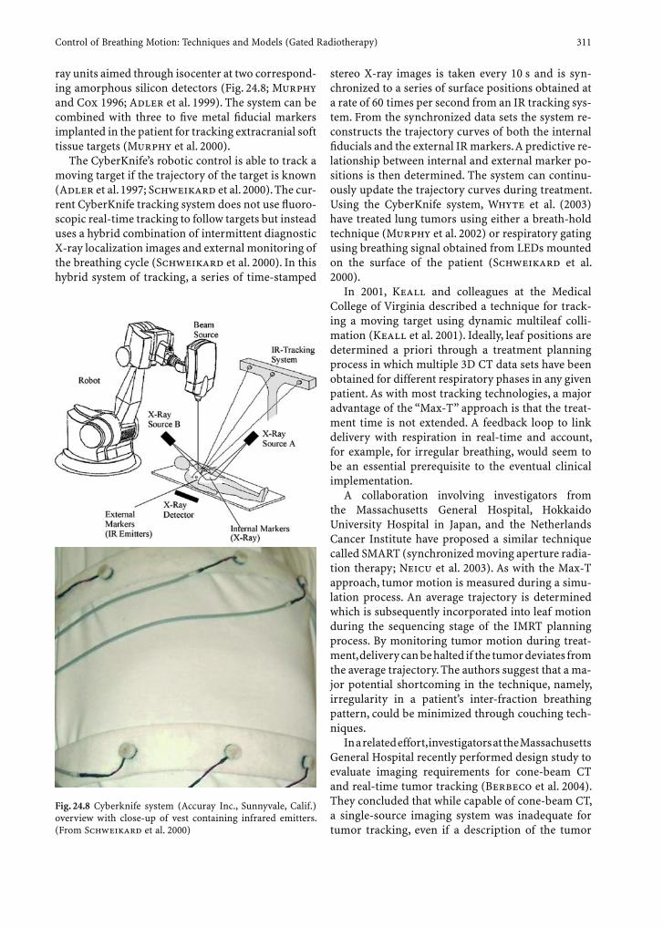
Control of Breathing Motion: Techniques and Models (Gated Radiotherapy) 311

ray units aimed through isocenter at two correspond-ing amorphous silicon detectors (Fig. 24.8; Murphy and Cox 1996; Adler et al. 1999). The system can be combined with three to fi ve metal fi ducial markers implanted in the patient for tracking extracranial soft tissue targets (Murphy et al. 2000).

The CyberKnife’s robotic control is able to track a moving target if the trajectory of the target is known (Adler et al. 1997; Schweikard et al. 2000). The cur-rent CyberKnife tracking system does not use fl uoro-scopic real-time tracking to follow targets but instead uses a hybrid combination of intermittent diagnostic X-ray localization images and external monitoring of the breathing cycle (Schweikard et al. 2000). In this hybrid system of tracking, a series of time-stamped

stereo X-ray images is taken every 10 s and is syn-chronized to a series of surface positions obtained at a rate of 60 times per second from an IR tracking sys-tem. From the synchronized data sets the system re-constructs the trajectory curves of both the internal fi ducials and the external IR markers. A predictive re-lationship between internal and external marker po-sitions is then determined. The system can continu-ously update the trajectory curves during treatment. Using the CyberKnife system, Whyte et al. (2003) have treated lung tumors using either a breath-hold technique (Murphy et al. 2002) or respiratory gating using breathing signal obtained from LEDs mounted on the surface of the patient (Schweikard et al. 2000).

In 2001, Keall and colleagues at the Medical College of Virginia described a technique for track-ing a moving target using dynamic multileaf colli-mation (Keall et al. 2001). Ideally, leaf positions are determined a priori through a treatment planning process in which multiple 3D CT data sets have been obtained for different respiratory phases in any given patient. As with most tracking technologies, a major advantage of the “Max-T” approach is that the treat-ment time is not extended. A feedback loop to link delivery with respiration in real-time and account, for example, for irregular breathing, would seem to be an essential prerequisite to the eventual clinical implementation.

A collaboration involving investigators from the Massachusetts General Hospital, Hokkaido University Hospital in Japan, and the Netherlands Cancer Institute have proposed a similar technique called SMART (synchronized moving aperture radia-tion therapy; Neicu et al. 2003). As with the Max-T approach, tumor motion is measured during a simu-lation process. An average trajectory is determined which is subsequently incorporated into leaf motion during the sequencing stage of the IMRT planning process. By monitoring tumor motion during treat-ment, delivery can be halted if the tumor deviates from the average trajectory. The authors suggest that a ma-jor potential shortcoming in the technique, namely, irregularity in a patient’s inter-fraction breathing pattern, could be minimized through couching tech-niques.

In a related effort, investigators at the Massachusetts General Hospital recently performed design study to evaluate imaging requirements for cone-beam CT and real-time tumor tracking (Berbeco et al. 2004). They concluded that while capable of cone-beam CT, a single-source imaging system was inadequate for tumor tracking, even if a description of the tumor

Fig. 24.8 Cyberknife system (Accuray Inc., Sunnyvale, Calif.) overview with close-up of vest containing infrared emitters. (From Schweikard et al. 2000)

312 T. D. Solberg et al.

motion had been previously obtained, and that im-age-guided and adaptive radiotherapy would be op-timally facilitated using a two-source system.

24.6 Dosimetric Consequences of Respiratory Motion

The subject of gated operation of modern radiother-apy treatment devices, and the dosimetric character-istics under such conditions, is one that has received little attention in the literature. The fi rst clinical in-vestigations were performed in Japan using a com-mercial linear accelerator (ML15MDX, Mitsubishi, Osaka, Japan; Ohara et al. 1989). A mask was used to detect ventilation and provide a respiration curve that was used to gate the linac. Beam stability, char-acterized by output, symmetry, and uniformity, was evaluated for gated and non-gated operation. Variations in measured dose of up to 5% were ob-served, although the monitor units delivered were quite low (≤10) compared with those typically re-quired in clinical practice. Additionally, deviations as large as 4.5% in cross- and in-plane uniformity were reported. Subsequently, the same group reported on the gated operation of a 500-MeV proton linac lo-cated operated at the University of Tsukuba, Japan (Ohara et al. 1989; Inada et al. 1992).

Kubo and Hill (1996) performed a similar inves-tigation using a commercial electron/photon linac (Varian Medical Systems, Palo Alto, Calif.). Several sensors were evaluated for their ability to monitor and accurately reproduce a human respiration pat-tern. These sensors were electronically interfaced with the linac for subsequent dosimetric character-ization. The beam was gated by tapping the gun delay circuit controlling the grid on the electron source. With 200 monitor units (MU) delivered at a rate of 240 MU/min, absolute dose differed by less than 0.1% when gating was performed with a duty cycle of 50%. Similarly, differences in symmetry were less than 1.2%. In addition to the obvious fact that dif-ferent linacs were used, the fact that these results are signifi cantly better than those reported by Ohara et al. (1989) is likely due to the small number of monitor units used in the earlier study. Ramsey et al. (1999) performed a subsequent investigation in which sev-eral delivery parameters were systematically evalu-ated. Dosimetric parameters were measured as moni-tor units were varied from 10 to 100 in fi ve segments of 2–20 MU pulses and with inter-pulse delays from

0.0 to 4.2 s. The dose rate remained fi xed at 320 MU/min. Results were quite similar to those of Kubo and Hill (1996), with maximum deviations of 0.8, 1.9, and 0.8% in output, fl atness and symmetry, respec-tively. The largest deviations were observed when the smallest number of monitor units was used.

Solberg et al. (2000) reported on the operation of a commercial gating implementation on a Novalis linear accelerator (BrainLAB AG, Heimstetten, Germany). Similar to the Varian units described pre-viously, gating was achieved through a three-pin con-nector that provides access to a 12-V DC signal to the MHOLDOFF/status bit on the console backplane. A beam inhibit is triggered whenever this bit is low. This bit toggles the initial position interlock (IPSN) inter-lock on the accelerator controller which subsequently halts both radiation and, in the case of dynamic treat-ment, leaf motion. Gating was performed under soft-ware control through a personal computer interfaced to the three-pin connector. In the study, monitor units were varied from 25 to 200 at gating frequen-cies from 0.2 to 1.0 Hz (at a constant 50% duty cycle). Two-dimensional dose maps were obtained using a 20¥20-cm2 amorphous-silicon imaging fl at-panel array (Scanditronix Medical/Wellhöfer Dosimetrie, Uppsala, Sweden) consisting of 256¥256 detector ele-ments. Frames were acquired every 80 ms and inte-grated to obtain an absolute dose map. Through the full dose-rate range (160–800 MU/min), no clinically signifi cant differences were observed in output, fl at-ness, or symmetry under gated operation.

Like the Varian unit, injection current on the Siemens ONCOR AvantGarde accelerator (Siemens Medical Solutions, Concord, Calif.) is regulated by a triode grid; however, in order to avoid in the temper-ature variations within the linac components, neither electron nor microwave generation are interrupted during the beam-off state under gated operation. Instead, the beam is interrupted by injecting elec-trons asynchronously with the microwave genera-tion. With this mechanism, energy dissipation, and therefore temperature variation in the linac compo-nents during gated operation, remains the same as during standard operation.

An investigation of the dosimetry characteristics under gated operation has been performed recently on the ONCOR accelerator at our institution. Ionization readings were recorded from a 0.6-cm3 chamber placed at a depth of 5 cm in solid water. Twenty-fi ve to 200 monitor units were delivered in non-gated op-eration and at gating frequencies ranging from 0.0625 to 0.50 Hz. A 50% duty cycle and dose rate of 300 MU/min were used. As with previous investigations, the

Control of Breathing Motion: Techniques and Models (Gated Radiotherapy) 313

largest deviations were observed when the smallest number of monitor units was used in combination with the high gating frequencies. With the exception of the 0.5 Hz/25 MU combination, output variations were all less than 0.5% (see Fig. 24.9).

to gate the beam during on the exhalation phase of a realistic respiratory cycle. In the case of dynamic wedge delivery, dosimetric differences between gated and non-gated operation were minimal except at the fi eld edges. Similarly, gating had a negligible effect on IMRT delivery.

In contrast, Solberg et al. (2000) observed signifi -cant dosimetric variations in gated wedged and in-tensity-modulated fi elds delivered through dynamic MLC, although the largest errors occurred in small spatial regions. The magnitude of these discrepan-cies was found to increase as smaller numbers of total monitors units were used and at higher gating fre-quencies (Fig. 24.10). A more in-depth investigation of these effects was performed recently Duan et al. (2003), who quantifi ed discrepancies between gated and non-gated delivery in a stationary phantom using both absolute dose and 2D dose distribution measurements. Output differences of up to 3.7% were observed in gated dynamic wedge fi elds as measured with a 0.6-cm3 ionization chamber. Additionally, dis-crepancies were observed in 2D dose distribution measurements. Dosimetric integrity under gated op-eration was found to correlate closely with dose rate, leaf speed, and frequency of beam interruptions. This was attributed primarily to the lag in leaf motion dur-ing dynamic delivery. Observations corresponded reasonably well with those of Solberg et al. (2000) shown in Fig. 24.9.

At least three groups have experimentally inves-tigated the dosimetric consequences of respiratory motion. Hugo et al. (2002) investigated the ability of a prototype gating system to reproduce non-gated IMRT dose distributions. A phantom capable of si-multaneous 2D movement (see Fig. 24.6) was set in motion using an analytical liver motion function ob-tained from the literature (Lujan et al. 1999). Under IMRT delivery, considerable dosimetric errors were observed between nonmoving and moving condi-tions (Fig. 24.11). Gating was found to substantially reduce these errors.

Duan et al. (2003) performed similar experiments using fi lm oriented perpendicular to the beam axis, in a phantom capable of 1D motion in the cranial–caudal direction. The Varian RPM system was used to generate gating signals. When respiratory gating was applied to the moving phantom (using a 25% duty cycle), differences between moving and stationary measurements were reduced from >10 mm distance errors and 5% dose errors to <1 mm and 1%.

Finally, Jiang et al. (2003) used an ionization chamber in solid water phantom placed on a mov-ing platform to characterize errors in IMRT delivery.

The dosimetric consequences of respiratory mo-tion are likely to be most signifi cant when dynamic delivery techniques, such as virtual wedge or inten-sity modulated radiotherapy (IMRT), are employed. These effects were fi rst quantifi ed in a theoretical study performed by Yu et al. (1998). In their inves-tigation, the authors suggested that under clinically realistic conditions, the interplay between the mo-tion-of-fi eld defi ning devices, such as multileaf col-limators (MLC) and target motion due to respira-tion, could produce intensity variations in the target anatomy as large as 480%. The authors pointed out, however, that the largest variations occurred in small spatial regions and would be signifi cantly reduced through the random smoothing process that occurs in fractionated delivery.

Bortfeld et al. (2002) expanded the investigation of the role of fractionation on the IMRT delivery/re-spiratory motion interplay. They concluded that intra-fraction effects rendered variations in the expected dose essentially independent of treatment technique.

Experimental investigations of the dosimetric variation associated with dynamic delivery and re-spiratory motion have been reported by several groups. Kubo and Wang (2000) evaluated the abil-ity of a Varian 2100C equipped with an 80-leaf MLC to deliver dynamic wedge and IMRT fi elds under gated operation. Several gating patterns were tested: one with an alternating 2-s beam on/beam off, an-other with an alternating 10-s beam on/beam off to simulate a breath-hold technique, and a third set

Fig. 24.9 Ratio of ionization chamber readings for the ONCOR accelerator under gated and non-gated operation

314 T. D. Solberg et al.

Fig. 24.11 Axial dose distributions for multifi eld IMRT delivery were obtained using fi lm in a moving phantom under non-gated (top) and gated (bottom) delivery. The measured 80, 50, and 20% isodose regions are shown in color-wash superimposed on results from treatment planning calculations (solid lines). Characterization was performed on the central axis (left), and 1 and 2 cm off axis (center and right, respectively). Regions where the acceptability criteria were exceeded, as measured by the multidimensional Gamma parameter (Low et al. 1998), are shown in the dark green overlay

Fig. 24.10 Average and maximum deviations of the 2D dose maps obtained in a plane perpendicular to the beam axis. Wedged fi elds were created by opening a leaf gap, and a sliding window technique was used for intensity-modulated radiotherapy (IMRT) delivery

Control of Breathing Motion: Techniques and Models (Gated Radiotherapy) 315

Motion was constrained to 1D sinusoidal movement, with an adjustable period and fi xed amplitude of 2 cm. While point dose errors of up to 30% for single and up to 18% for multiple fi elds were observed, the authors suggested that fractionated delivery would signifi cantly reduce the magnitude of these errors. Nevertheless, they pointed out that further study was needed to characterize the effects in normal/critical tissue outside of the target volume.

24.7 Conclusion

For continued clinical gains in the practice of radio-therapy, management of breathing motion is essen-tial. The problem of organ motion in radiotherapy is complex; thus, interventions to reduce organ-mo-tion-related uncertainties require effort, expertise, and collaboration from many disciplines. The ap-plication of image-guidance techniques, i.e., image-guided radiotherapy, will play an increasing impor-tant role in developing new and improved delivery techniques, i.e., adaptive radiotherapy. With some anecdotal clinical evidence and many potentially benefi cial but unproven technologies under devel-opment and on the horizon, it is essential to place equal emphasis on the planning and implementation of prospective clinical trials.

References

Adler JR Jr, Chang SD, Murphy MJ et al. (1997) The Cyberknife: a frameless robotic system for radiosurgery. Stereotact Funct Neurosurg 69:124–128

Adler JR Jr, Murphy MJ, Chang SD et al. (1999) Image-guided robotic radiosurgery. Neurosurgery 44:1299–1306

Allen AM, Siracuse KM, Hayman JA et al. (2004) Evalua-tion of the infl uence of breathing on the movement and modeling of lung tumors. Int J Radiat Oncol Biol Phys 58:1251–1257

Aruga T, Itami J, Aruga M et al. (2000) Target volume defi -nition for upper abdominal irradiation using CT scans obtained during inhale and exhale phases. Int J Radiat Oncol Biol Phys 48:465–469

Axelsonn P, Johnsson R, Stromqvist B (1996) Mechanics of the external fi xation test an the lumbar spine: a roentgen stereophotogrammetric analysis. Spine 21:330–333

Balter JM, Ten Haken RK, Lawrence TS et al. (1996) Uncertain-ties in CT-based treatment plans due to patient breathing. Int. J. Radiation Oncology Biol. Phys. 36:167–174

Balter JM, Lam KL, McGinn CJ et al. (1998) Improvement of CT-based treatment-planning models of abdominal tar-

gets using static exhale imaging. Int. J. Radiation Oncol-ogy Biol. Phys. 41:939-943

Balter JM, Dawson LA, Kazanijian S et al. (2001) Determina-tion of ventilatory liver movement via radiographic eval-uation of diaphragm position, Int. J. Radiation Oncology Biol. Phys. 51:267–270

Baroni G, Ferrigno G, Orecchia R et al. (2000) Real-time three-dimensional motion analysis for patient position-ing verifi cation. Radiother Oncol 54:21-7

Berbeco RI, Jiang SB, Sharp GC et al. (2004) Integrated radio-therapy imaging system (IRIS): design considerations of tumour tracking with linac gantry-mounted diagnostic X-ray systems with fl at-panel detectors. Phys Med Biol 49:243–255

Blomgren H, Lax I, Naslund I et al. (1995) Stereotactic high dose fraction radiation therapy of extracranial tumors using an accelerator. Clinical experience of the fi rst thirty-one patients. Acta Oncol 34:861–870

Blomgren H, Lax I, Goranson H et al. (1999) Radiosurgery for tumors in the body: clinical experience using a new method. J Radiosurg 2:239–245

Bortfeld T, Jokivarsi K, Goitein M et al. (2002) Effects of intra-fraction motion on IMRT dose delivery: statistical analy-sis and simulation. Phys Med Biol 47:2203–2220

Bova FJ, Buatti JM, Friedman WA et al. (1997) The Uni-versity of Florida frameless high-precision stereotac-tic radiotherapy system. Int J Radiat Oncol Biol Phys 38:875–882

Brugmans MJ, van der Horst A, Lebesque JV et al. (1999) Beam intensity modulation to reduce the fi eld sizes for conformal irradiation of lung tumors: a dosimetric study. Int J Radiat Oncol Biol Phys 43:893–904

Carman AB, Milburn PD (1997) Conjugate imagery in the automated reproduction of three dimensional coordi-nates from two dimensional coordinate data. J Biomech 30:733–736

Chen QS, Weinhous MS, Deibel FC et al. (2001) Fluoroscopic study of tumor motion due to breathing: facilitating pre-cise radiation therapy for lung cancer patients. Med Phys 28:1850–1856

De Koste JRV, Lagerwaard FJ, Schuchhard-Schipper RH et al. (2001) Dosimetric consequences of tumor mobility in radiotherapy of stage I non-small cell lung cancer: an analysis of data generated using “slow” CT scans. Radio-ther Oncol 61:93–99

De Koste JRV, Lagerwaard FJ, de Boer HCJ et al. (2003) Are multiple CT scans required for planning curative radio-therapy in lung tumors of the lower lobe? Int J Radiat Oncol Biol Phys 55:1394–1399

Dhanantwari AC, Stergiopoulos S, Iakovidis I (2001a) Cor-recting organ motion artifacts in X-ray CT medical imag-ing systems by adaptive processing. I. Theory Med Phys 28:1562–1576

Dhanantwari AC, Stergiopoulos S, Zamboglou N et al. (2001b) Correcting organ motion artifacts in X-ray CT systems based on tracking of motion phase by the spa-tial overlap correlator. II. Experimental study. Med Phys 28:1577–1596

Duan J, Shen S, Fiveash JB et al. (2003) Dosimetric effect of respiration-gated beam on IMRT delivery. Med Phys 30:2241–2252

Ekberg L, Holmberg O, Wittgren L et al. (1998) What margins should be added to the clinical target volume in radio-

316 T. D. Solberg et al.

therapy treatment planning for lung cancer? Radiother Oncol 48:71–77

Farre R, Montserrat JM, Rotget M et al. (1998) Accuracy of thermistors and thermocouples as fl ow-measuring devices for detecting hypopnoeas. Eur Respir J 11:179–182

Frazier RC, Vicini FA, Sharpe MB et al. (2004) Impact of breathing motion on whole breast radiotherapy: a dosi-metric analysis using active breathing control. Int J Radiat Oncol Biol Phys 58:1041–1047

Ford EC, Mageras GS, Yorke E et al. (2002) Evaluation of respiratory movement during gated radiotherapy using fi lm and electronic portal imaging. Int J Radiat Oncol Biol Phys 52:522–531

Ford EC, Mageras GS, Yorke E et al. (2003) Respiration-cor-related spiral CT: a method of measuring respiratory-induced anatomic motion for radiation treatment plan-ning. Med Phys 30:88–97

George R, Keall P, Chung T et al. (2004) Dynamic multileaf collimation and three-dimensional verifi cation in IMRT. In: Yi BY, Ahn SD, Choi EK, Ha SW (eds) The use of com-puters in radiation therapy. Jeong Publishing, Seoul, pp 437–441

Giraud P, De Rycke Y, Dubray B et al. (2001) Conformal radio-therapy (CRT) planning for lung cancer: analysis of intra-thoracic organ motion during extreme phases of breath-ing. Int J Radiat Oncol Biol Phys 51:1081–1092

Hanley J, Debois MM, Mah D et al. (1999) Deep inspiration breath-hold technique for lung tumors: the potential value of target immobilization and reduced lung density in dose escalation. Int J Radiat Oncol Biol Phys 45:603–611

Herfarth KK, Debus J, Lohr F et al. (2000) Extracranial ste-reotactic radiation therapy: set-up accuracy of patients treated for liver metastases. Int J Radiat Oncol Biol Phys 46:329–335

Hugo GD, Agazaryan N, Solberg TD (2002) An evaluation of gating window size, delivery method, and composite fi eld dosimetry of respiratory-gated IMRT. Med Phys 29:2517–2525

Hugo GD, Agazaryan N, Solberg TD (2003) The effects of tumor motion on planning and delivery of respiratory-gated IMRT. Med Phys 30:1052–1066

Inada T, Tsuji H, Hayakawa Y et al. (1992) Proton irradiation synchronized with respiratory cycle. Nippon Acta Radiol 52:1161–1167

Intensity Modulated Radiation Therapy Collaborative Work-ing Group (2001) Intensity-modulated radiotherapy: cur-rent status and issues of interest. Int J Radiat Oncol Biol Phys 51:880–914

Jiang SB, Pope C, Al Jarrah MK et al. (2003) An experimental investigation on intra-fractional organ motion effects in lung IMRT treatments. Phys Med Biol 48:1773–1784

Johnson CA, Keltner JL, Krohn MA et al. (1979) Photogram-metry of the optic disc in glaucoma and ocular hyperten-sion with simultaneous stereo photography. Invest Oph-thal Vis Sci 18:1252–1263

Keall PJ, Kini VR, Vedam SS et al. (2001) Motion adaptive X-ray therapy: a feasibility study. Phys Med Biol 46:1–10

Keall PJ, Kini VR, Vedam SS et al. (2002) Potential radiother-apy improvements with respiratory gating. Australas Phys Eng Sci Med 25:1–6

Keall PJ, Starkschall G, Shukla H et al. (2004) Acquiring 4D thoracic CT scans using a multislice helical method. Phys Med Biol 49:2053–2067

Kearfoot K, Juang RJ, Marzke MW (1993) Implementation of digital stereo imaging for analysis of metaphyses and joints in skeletal collections. Med Biol Eng Computing 31:149–156

Kini VR, Keall PJ, Vedam SS et al. (2000) Preliminary results from a study of a respiratory motion tracking system: underestimation of target volume with conventional CT simulation. Int J Radiat Oncol Biol Phys 48:164

Kini VR, Vedam SS, Keall PJ et al. (2003) Patient training in respiratory-gated radiotherapy. Med Dosim 28:7–11

Kitamura K, Shirato H, Seppenwoolde Y et al. (2002a) Three-dimensional intrafractional movement of the prostate measured during real-time tumor-tracking radiotherapy in supine and prone treatment positions. Int J Radiat Oncol Biol Phys 53:1117–1123

Kitamura K, Shirato H, Seppenwoolde Y et al. (2002b) Three-dimensional intrafractional movement of prostate mea-sured during real-time tumor-tracking radiotherapy in supine and prone treatment positions. Int J Radiat Oncol Biol Phys 53:1117–1123

Kitamura K, Shirato H, Shimizu S et al. (2002c) Registration accuracy and possible migration of internal fi ducial gold marker implanted in prostate and liver treated with real-time tumor-tracking radiation therapy (RTRT). Radio-ther Oncol 62:275–281

Kitamura K, Shirato H, Seppenwoolde Y et al. (2003) Tumor location, cirrhosis, and surgical history contribute to tumor movement in the liver, as measured during stereo-tactic irradiation using a real-time tumor-tracking radio-therapy system. Int J Radiat Oncol Biol Phys 56:221–228

Ko Y, Yi B, Ahn S et al. (2004) Immobilization effect of air injected blanket for abdomen fi xation. In: Yi BY, Ahn SD, Choi EK, Ha SW (eds) The use of computers in radiation therapy. Jeong Publishing, Seoul, pp 421–423

Kubo HD, Hill BC (1996) Respiration gated radiotherapy treatment: a technical study. Phys Med Biol 41:83–91

Kubo HD, Wang L (2000) Compatibility of Varian 2100C gated operations with enhanced dynamic wedge and IMRT dose delivery. Med Phys 27:1732–1738

Kubo HD, Len PM, Minohara S et al. (2000) Breathing-syn-chronized radiotherapy program at the University of Cali-fornia Davis Cancer Center. Med Phys 27:346–353

Kwa SLS, Lebesque JV, Theuws JCM et al. (1998) Radiation pneumonitis as a function of meal lung dose: an analysis of pooled data of 540 patients. Int J Radiat Oncol Biol Phys 42:1–9

Lagerwaard FJ, de Koste JRV, Nijssen-Visser MRJ et al. (2001) Multiple “slow” CT scans for incorporating lung tumor mobility in radiotherapy planning. Int J Radiat Oncol Biol Phys 51:932–937

Lawrence TS, Robertson JM, Anscher MS et al. (1995) Hepatic toxicity resulting from cancer treatment. Int J Radiat Oncol Biol Phys 31:1237–1248

Lax I, Blomgren H, Naslund I et al. (1994) Stereotactic radio-therapy of malignancies in the abdomen. Methodological aspects. Acta Oncol 33:677–683

Lindemann J, Leiacker R, Rettinger G et al. (2002) Nasal mucosal temperature during respiration. Clin Otolaryn-gol 27:135–139

Low DA, Harms WB, Mutic S et al. (1998) A technique for the quantitative evaluation of dose distributions. Med Phys 25:656–661

Low D, Wahab S, El Naqa I et al. (2003a) Four-dimensional

Control of Breathing Motion: Techniques and Models (Gated Radiotherapy) 317

computed tomography using a 16-slice scanner. Med Phys 30:1506

Low D, Nystrom M, Kalinin E et al. (2003b) A method for the reconstruction of four-dimensional synchronized CT scans acquired during free breathing. Med Phys 30:1254–1263

Lu W, Mackie TR (2002) Tomographic motion detection and correction directly in sinogram space. Phys Med Biol 47:1267–1284

Lujan AE, Larsen EW, Balter JM et al. (1999) A method for incorporating organ motion due to breathing into 3D dose calculations. Med Phys 26:715–720

Mageras GS, Yorke E (2004) Deep inspiration breath hold and respiratory gating strategies for reducing organ motion in radiation treatment. Semin Radiat Oncol 14:65–75

Mageras GS, Yorke E, Rosenzweig K et al. (2001) Fluoroscopic evaluation of diaphragmatic motion reduction with a respiratory gated radiotherapy system. J Appl Clin Med Phys 2:191–200

Mah D, Hanley J, Rosenzweig KE et al. (2000) Technical aspects of the deep inspiration breath-hold technique in the treatment of thoracic cancer. Int J Radiat Oncol Biol Phys 48:1175–1185

Marks MK, South M, Carter BG (1995) Measurement of respi-ratory rate and timing using a nasal thermocouple. J Clin Monit 11:159–164

Martel MK, Ten Haken RK, Hazuka MB et al. (1999) Esti-mation of tumor control probability model parameters from 3-D dose distributions of non-small cell lung cancer patients. Lung Cancer 24:31–37

Mehta M, Scrimger R, Mackie R et al. (2001) A new approach to dose escalation in non-small-cell lung cancer. Int J Radiat Oncol Biol Phys 49:23–33

Menke M, Hirschfeld F, Mack T et al. (1994) Stereotactically guided fractionated radiotherapy: technical aspects. Int J Radiat Oncol Biol Phys 29:1147–1155

Minohara S, Kanai T, Endo M et al. (2000) Respiratory gated irradiation system for heavy-ion radiotherapy. Int J Radiat Oncol Biol Phys 47:1097–1103

Mori S, Endo M, Tsunoo T et al. (2004) Physical performance evaluation of a 256-slice CT-scanner for four-dimensional imaging. Med Phys 31:1348–1356

Morita K, Fuwa N, Suzuki M et al. (1997) Radical radiother-apy for medically inoperable non-small cell lung cancer in clinical stage I: a retrospective analysis of 149 patients. Radiother Oncol 42:31–36

Murphy MJ, Cox RS (1996) The accuracy of dose localization for an image-guided frameless radiosurgery system. Med Phys 23:2043–2049

Murphy MJ, Adler JR Jr, Bodduluri M et al. (2000) Image-guided radiosurgery for the spine and pancreas. Comput Aided Surg 5:278–288

Murphy MJ, Martin D, Whyte R et al. (2002) The effective-ness of breath-holding to stabilize lung and pancreas tumors during radiosurgery. Int J Radiat Oncol Biol Phys 53:475–482

Nagata Y, Negoro Y, Aoki T et al. (2003) Clinical outcomes of 3D conformal hypofractionated single high-dose radiotherapy for one or two lung tumors using a ste-reotactic body frame. Int J Radiat Oncol Biol Phys 52:1041–1046

Narayan S, Henning GT, Ten Haken RK et al. (2004) Results following treatment to doses of 92.4 or 102.9 Gy on a

phase I dose escalation study for non-small cell lung cancer. Lung Cancer 44:79–88

Negoro Y, Nagata Y, Aoki T et al. (2001) The effectiveness of an immobilization device in conformal radiotherapy for lung tumor: reduction of respiratory tumor movement and evaluation of the daily setup accuracy. Int J Radiat Oncol Biol Phys 50:889–898

Neicu T, Shirato H, Seppenwoolde Y et al. (2003) Synchro-nized moving aperture radiation therapy (SMART): aver-age tumour trajectory for lung patients. Phys Med Biol 48:587–598

Norman RG, Ahmed MM, Walsleben TA et al. (1997) Detec-tion of respiratory events during NPSG: nasal cannula/pressure sensor versus thermistor. Sleep 20:1175–1184

Ohara K, Okumura T, Akisada M et al. (1989) Irradiation syn-chronized with respiration gate. Int J Radiat Oncol Biol Phys 17:853–857

Ozhasoglu C, Murphy MJ (2002) Issues in respiratory motion compensation during external-beam radiotherapy. Int J Radiat Oncol Biol Phys 52:1389–1399

Pan T, Lee T-Y, Rietzel E et al. (2004) 4D-CT imaging of a volume infl uenced by respiratory motion on multi-slice CT. Med Phys 31:333–340

Peterson B, Palmerud G (1996) Measurement of upper extremity orientation by video stereometry system. Med Biol Eng Computing 34:149–154

Ramsey CR, Cordrey IL, Oliver AL (1999) comparison of beam characteristics for gated and nongated clinical X-ray beams. Med Phys 26:2086–2091

Reed GB, Cox AJ (1966) The human liver after radiation injury. Am J Pathol 48:597–612

Remouchamps VM, Letts N, Vicini FA et al. (2003a) Ini-tial clinical experience with moderate deep-inspiration breath hold using an active breathing control device in the treatment of patients with left-sided breast cancer using external beam radiation therapy. Int J Radiat Oncol Biol Phys 56:704–715

Remouchamps VM, Letts N, Yan D et al. (2003b) Three-dimen-sional evaluation of intra- and interfraction immobiliza-tion of lung and chest wall using active breathing control: a reproducibility study with breast cancer patients. Int J Radiat Oncol Biol Phys 57:968–978

Remouchamps VM, Vicini FA, Sharpe MB et al. (2003c) Sig-nifi cant reductions in heart and lung doses using deep inspiration breath hold with active breathing control and intensity-modulated radiation therapy for patients treated with locoregional breast irradiation. Int J Radiat Oncol Biol Phys 55:392–406

Ries LAG, Eisner MP, Kosary CL et al. (eds) (2004) NCI Sur-veillance, Epidemiology and End Results. SEER Cancer Statistics Review, 1975–2001, National Cancer Institute. Bethesda, Maryland

Rietzel E, Chen GT, Doppke KP et al. (2003) 4D computed tomography for treatment planning. Int J Radiat Oncol Biol Phys 57:S232–S233

Ritchie CJ, Hsieh J, Gard MF et al. (1994) Predictive respira-tory gating: a new method to reduce motion artifacts on CT scans. Radiology 190:847–852

Robertson JM, Lawrence TS, Andrews JC et al. (1997a) Long-term results of hepatic artery fl uorodeoxyuridine and conformal radiation therapy for primary hepatobiliary cancers. Int J Radiat Oncol Biol Phys 37:325–330

Robertson JM, Ten Haken RK, Hazuka MB et al. (1997b) Dose

318 T. D. Solberg et al.

escalation for non-small cell lung cancer using conformal radiation therapy. Int J Radiat Oncol Biol Phys 37:1079–1085

Roof KS, Fidias P, Lynch TJ et al. (2003) Radiation dose esca-lation in limited-stage small-cell lung cancer. Int J Radiat Oncol Biol Phys 57:701–708

Rosenzweig KE, Hanley J, Mah D et al. (2000) The deep inspi-ration breath-hold technique in the treatment of inoper-able non-small-cell lung cancer. Int J Radiat Oncol Biol Phys 48:81–87

Ross C, Hussey DH, Pennington EC et al. (1990) Analysis of movement on intrathoracic neoplasm using ultrafast computerized tomography. Int J Radiat Oncol Biol Phys 18:671–677

Ruschin M, Sixel KE (2002) Integration of digital fl uoroscopy with CT-based radiation therapy planning of lung tumors. Med Phys 29:1698–1709

Sang-Wook Lee S, Eun Kyung Choi EK, Heon Joo Park HJ et al. (2003) Stereotactic body frame based fractionated radiosurgery on consecutive days for primary or meta-static tumors in the lung. Lung Cancer 40:309–315

Sato M, Uematsu M, Yamamoto F et al. (1998) Feasibility of frameless stereotactic high-dose radiation therapy for pri-mary or metastatic liver cancer. J Radiosurg 1:233–240

Schlegel W, Pastyr O, Bortfeld T et al. (1993) Stereotacti-cally guided fractionated radiotherapy: technical aspects. Radiother Oncol 29:197–204

Schweikard A, Glosser G, Bodduluri M et al. (2000) Robotic motion compensation for respiratory movement during radiosurgery. Comput Aided Surg 5:263–277

Selvik G (1990) Roentgen stereophotogrammetric analysis. Acta Radiol 31:113–126

Seppenwoolde Y, Shirato H, Kitamura K et al. (2002) Precise and real-time measurement of 3D tumor motion in lung due to breathing and heartbeat, measured during radio-therapy. Int J Radiat Oncol Biol Phys 53:822–834

Shimizu S, Shirato H, Ogura S et al. (2001) Detection of lung tumor movement in real-time tumor-tracking radiother-apy. Int J Radiat Oncol Biol Phys 51:304–310

Shirato H, Harada T, Harabayashi T et al. (2003) Feasibil-ity of insertion/implantation of 2.0-mm-diameter gold internal fi ducial markers for precise setup and real-time tumor tracking in radiotherapy. Int J Radiat Oncol Biol Phys 56:240–247

Shirato H, Shimizu S, Kitamura K et al. (2000a) Four-dimen-sional treatment planning and fl uoroscopic real-time tumor tracking radiotherapy for moving tumor. Int J Radiat Oncol Biol Phys 48:435–442

Shirato H, Shimizu S, Kunieda T et al. (2000b) Physical aspects of a real-time tumor-tracking system for gated radiotherapy. Int J Radiat Oncol Biol Phys 48:1187–1195

Sixel K, Ruschin M, Cheung PC (2001) Integration of digital fl uoroscopy with CT simulation: patient specifi c planning target volumes. Int J Radiat Oncol Biol Phys 51 (S1):122–123

Sixel KE, Ruschin M, Tirona R et al. (2003) Digital fl uoros-copy to quantify lung tumor motion: potential for patient-specifi c planning target volumes. Int J Radiat Oncol Biol Phys 57:717–723

Solberg TD, Paul TJ, Agazaryan N et al. (2000) Dosimetry of gated intensity modulated radiotherapy. In: Schlegel W, Bortfeld T (eds) The use of computers in radiation ther-apy. Springer, Berlin Heidelberg New York, pp 286–288

Stevens CW, Munden RF, Forster KM et al. (2001) Respira-tory-driven lung tumor motion is independent of tumor size, tumor location, and pulmonary function. Int J Radiat Oncol Biol Phys 51:62–68

Stromberg JS, Sharpe MB, Kim LH et al. (2000) Active breathing control (ABC) for Hodgkin’s disease: reduction in normal tissue irradiation with deep inspiration and implications for treatment. Int J Radiat Oncol Biol Phys 48:797–806

Stroom JC, Heijmen BJ (2002) Geometrical uncertainties, radiotherapy planning margins, and the ICRU-62 report. Radiother Oncol 64:75–83

Suit HD, Becht J, Leong J et al. (1988) Potential for improve-ment in radiation therapy. Int J Radiat Oncol Biol Phys 14:777–786

Taguchi K (2003) Temporal resolution and the evaluation of candidate algorithms for four-dimensional CT. Med Phys 30:640–650

Ten Haken RK, Balter JM, Marsh LH et al. (1997) Potential benefi ts of eliminating planning target volume expansions for patient breathing in the treatment of liver tumors. Int J Radiat Oncol Biol Phys 38:613–617

Tsunashima Y, Sakae T, Shioyama Y et al. (2004) Correla-tion between the respiratory waveform measured using a respiratory sensor and 3D tumor motion in gated radio-therapy. Int J Radiat Oncol Biol Phys. 60:951–958

Vedam SS, Keall PJ, Kini VR et al. (2001) Determining parameters for respiration-gated radiotherapy. Med Phys 28:2139–2146

Vedam SS, Keall PJ, Kini VR et al. (2003) Acquiring a four-dimensional computed tomography dataset using an external respiratory signal. Phys Med Biol 48:45–62

Vedam SS, Keall PJ, Docef A et al. (2004) Predicting respira-tory motion for four-dimensional radiotherapy. Med Phys 31:2274–2283

Verellen D, Soete G, Linthout N et al. (2003) Quality assurance of a system for improved target localization and patient set-up that combines real-time infrared tracking and ste-reoscopic X-ray imaging. Radiother Oncol 67:129–141

Wagman R, Yorke E, Ford E et al. (2003) Respiratory gating for liver tumors: use in dose escalation. Int J Radiat Oncol Biol Phys 55:659–668

Wahab S, Low D, El Naqa I et al. (2003) Use of four-dimen-sional computed tomography in conformal therapy plan-ning for lung cancer. Med Phys 30:1364

Wang LT, Solberg TD, Medin PM et al. (2001) Infrared patient positioning for stereotactic radiosurgery of extracranial tumors. Comput Biol Med 31:101–111

Waters K, Terzopoulos D (1992) The computer synthesis of expressive faces. Philos Trans R Soc London Series B Biol Sci 335:87–93

Whyte RI, Crownover R, Murphy MJ et al. (2003) Stereotac-tic radiosurgery for lung tumors: preliminary report of a phase I trial. Ann Thorac Surg 75:1097–1101

Willett CG, Linggood RM, Stracher MA et al. (1987) The effect of the respiratory cycle on mediastinal and lung dimen-sions in Hodgkin’s disease. Implications for radiotherapy gated to respiration. Cancer 60:1232–1237

Willner J, Baier K, Caragiani E et al. (2002) Dose, volume, and tumor control predictions in primary radiotherapy of non-small-cell lung cancer. Int J Radiat Oncol Biol Phys 52:382–389

Wilson EM, Williams FJ, Lyn BE et al. (2003) Validation of

Control of Breathing Motion: Techniques and Models (Gated Radiotherapy) 319

active breathing control in patients with non-small-cell lung cancer to be treated with CHARTWEL. Int J Radiat Oncol Biol Phys 57:864–874

Wong JW, Sharpe MB, Jaffray DA et al. (1997) The use of active breathing control (ABC) to minimize breathing motion during radiation therapy. Int J Radiat Oncol Biol Phys 39:164 (abstract)

Wong JW, Sharpe MB, Jaffray DA et al. (1999) The use of active breathing control (ABC) to reduce margin for breathing motion. Int J Radiat Oncol Biol Phys 44:911–919

Wulf J, Hädinger U, Oppitz U et al. (2001) Stereotactic radio-

therapy of targets in the lung and liver. Strahlenther Onkol 177:645–655

Xiong C, Sjoberg BJ, Sveider P et al. (1993) Problems in the timing of respiration with the nasal thermistor technique. J Am Soc Echocardiogr 6:210–216

Yu CX, Jaffray DA, Wong JW (1998) The effects of intra-frac-tion organ motion on the delivery of dynamic intensity modulation. Phys Med Biol 43:91–104

Zhang T, Jeraj R, Keller H et al. (2004) Treatment plan opti-mization incorporating respiratory motion. Med Phys 31:1576–1586

Image-Guided/Adaptive Radiotherapy 321

25 Image-Guided/Adaptive Radiotherapy

Di Yan

D. Yan, D.Sc.Director, Clinical Physics Section, Department of Radiation Oncology, William Beaumont Hospital, Royal Oak, MI 48073-6769, USA

CONTENTS

25.1 Introduction 32125.2 Temporal Variation of Patient/Organ Shape and Position 32325.3 Imaging and Verifi cation 32425.3.1 Verifi cation with Radiographic Imaging 32425.3.2 Verifi cation with Fluoroscopic Imaging 32525.3.3 Verifi cation with CT Imaging 32525.4 Estimation and Evaluation 32725.4.1 Parameter Estimation for a Stationary Temporal Variation Process 32725.4.2 Parameter Estimation for a Non-stationary Temporal Variation Process 32825.4.3 Estimation of Cumulative Dose 32925.5 Design of Adaptive Planning and Adjustment 33025.5.1 Design Objectives 33025.5.2 Adaptive Planning and Adjustment Parameters 33025.5.3 Adaptive Planning and Adjustment Parameter and Schedule: Selection and Modifi cation 33025.6 Adaptive Planning and Adjustment 33225.6.1 Indirect Method 33225.6.2 Direct Method 33325.7 Adaptive Treatment Protocol 33425.7.1 Example 1: Image-Guided/Adaptive Radiotherapy for Prostate Cancer 33425.7.2 Example 2: Image-Guided/Adaptive Radiotherapy for NSCLC 33425.8 Summary 335 References 335

25.1 Introduction

Adaptive radiotherapy is a treatment technique that can systematically improve its treatment plan in re-sponse to patient/organ temporal variations observed during the therapy process. Temporal variations in radiotherapy process can be either patient/organ

geometry or dose-response related. Examples of the former include inter- and intra-treatment variations of patient/organ shape and positions caused by pa-tient setup, beam placement, and patient organ physi-ological motion and deformation. Examples of dose response characteristics include the variations of size and location of tumor hypoxic volume, the appar-ent tumor growth fraction, and normal tissue dam-age/repair kinetics. Furthermore, tumor and normal organ dose response also induce changes in tissue shape and positions.

This chapter focuses on the use of adaptive strategies to manage patient/organ shape and posi-tion related temporal variations; however, the con-cepts of adaptive radiotherapy can be extended to a much broader range, including the management in temporal variations of patient/organ biology.

It is generally accepted that temporal variations are the predominant sources of treatment uncertainty in conventional radiation treatment. Numerous imag-ing studies have demonstrated that substantial tem-poral variations of patient/organ shape and position could occur during a typical radiotherapy course (Brierley et al. 1994; Davies et al. 1994; Halverson et al. 1991; Marks and Haus 1976; Moerland et al. 1994; Nuyttens et al. 2001; Roeske et al. 1995; Ross et al. 1990). Consequently, the radiation dose deliv-ered to the target and a critical normal organ adja-cent to the target can signifi cantly deviate from that calculated in the pre-treatment planning. This devia-tion causes a time-dependent, or temporal, variation in the organ-dose distribution, consisting of both dose variation per treatment fraction and cumulative dose variation in each subvolume of the organ, and results in major treatment uncertainties. These un-certainties induce fundamental obstacles to assuring treatment quality and understanding the normal tis-sue dose response, thereby hindering reliable treat-ment optimization.

Temporal variations in patient/organ shape and position during the radiotherapy course can be sepa-rated into a systematic component and a random component. The systematic component represents

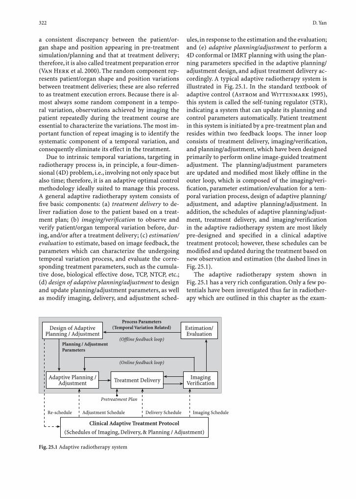
322 D. Yan

a consistent discrepancy between the patient/or-gan shape and position appearing in pre-treatment simulation/planning and that at treatment delivery; therefore, it is also called treatment preparation error (Van Herk et al. 2000). The random component rep-resents patient/organ shape and position variations between treatment deliveries; these are also referred to as treatment execution errors. Because there is al-most always some random component in a tempo-ral variation, observations achieved by imaging the patient repeatedly during the treatment course are essential to characterize the variations. The most im-portant function of repeat imaging is to identify the systematic component of a temporal variation, and consequently eliminate its effect in the treatment.

Due to intrinsic temporal variations, targeting in radiotherapy process is, in principle, a four-dimen-sional (4D) problem, i.e., involving not only space but also time; therefore, it is an adaptive optimal control methodology ideally suited to manage this process. A general adaptive radiotherapy system consists of fi ve basic components: (a) treatment delivery to de-liver radiation dose to the patient based on a treat-ment plan; (b) imaging/verifi cation to observe and verify patient/organ temporal variation before, dur-ing, and/or after a treatment delivery; (c) estimation/evaluation to estimate, based on image feedback, the parameters which can characterize the undergoing temporal variation process, and evaluate the corre-sponding treatment parameters, such as the cumula-tive dose, biological effective dose, TCP, NTCP, etc.; (d) design of adaptive planning/adjustment to design and update planning/adjustment parameters, as well as modify imaging, delivery, and adjustment sched-

ules, in response to the estimation and the evaluation; and (e) adaptive planning/adjustment to perform a 4D conformal or IMRT planning with using the plan-ning parameters specifi ed in the adaptive planning/adjustment design, and adjust treatment delivery ac-cordingly. A typical adaptive radiotherapy system is illustrated in Fig. 25.1. In the standard textbook of adaptive control (Astrom and Wittenmark 1995), this system is called the self-tuning regulator (STR), indicating a system that can update its planning and control parameters automatically. Patient treatment in this system is initiated by a pre-treatment plan and resides within two feedback loops. The inner loop consists of treatment delivery, imaging/verifi cation, and planning/adjustment, which have been designed primarily to perform online image-guided treatment adjustment. The planning/adjustment parameters are updated and modifi ed most likely offl ine in the outer loop, which is composed of the imaging/veri-fi cation, parameter estimation/evaluation for a tem-poral variation process, design of adaptive planning/adjustment, and adaptive planning/adjustment. In addition, the schedules of adaptive planning/adjust-ment, treatment delivery, and imaging/verifi cation in the adaptive radiotherapy system are most likely pre-designed and specifi ed in a clinical adaptive treatment protocol; however, these schedules can be modifi ed and updated during the treatment based on new observation and estimation (the dashed lines in Fig. 25.1).

The adaptive radiotherapy system shown in Fig. 25.1 has a very rich confi guration. Only a few po-tentials have been investigated thus far in radiother-apy which are outlined in this chapter as the exam-

Clinical Adaptive Treatment Protocol

(Schedules of Imaging, Delivery, & Planning / Adjustment)

Pretreatment Plan

Re-schedule Imaging ScheduleDelivery ScheduleAdjustment Schedule

Design of Adaptive Planning / Adjustment

Estimation/Evaluation

Adaptive Planning / Adjustment Treatment Delivery Imaging

Verifi cation

Process Parameters(Temporal Variation Related)

(Offl ine feedback loop)Planning / AdjustmentParameters

(Online feedback loop)

Fig. 25.1 Adaptive radiotherapy system

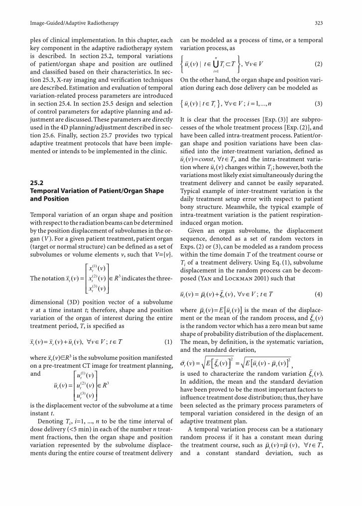
Image-Guided/Adaptive Radiotherapy 323

ples of clinical implementation. In this chapter, each key component in the adaptive radiotherapy system is described. In section 25.2, temporal variations of patient/organ shape and position are outlined and classifi ed based on their characteristics. In sec-tion 25.3, X-ray imaging and verifi cation techniques are described. Estimation and evaluation of temporal variation-related process parameters are introduced in section 25.4. In section 25.5 design and selection of control parameters for adaptive planning and ad-justment are discussed. These parameters are directly used in the 4D planning/adjustment described in sec-tion 25.6. Finally, section 25.7 provides two typical adaptive treatment protocols that have been imple-mented or intends to be implemented in the clinic.

25.2 Temporal Variation of Patient/Organ Shape and Position

Temporal variation of an organ shape and position with respect to the radiation beams can be determined by the position displacement of subvolumes in the or-gan (V ). For a given patient treatment, patient organ (target or normal structure) can be defi ned as a set of subvolumes or volume elements v, such that V={v}.

The notation vx v

x vx vx v

Rt

t

t

t

( )( )( )( )

( )

( )

( )

=⎡

⎣

⎢⎢⎢

⎤

⎦

⎥⎥⎥∈

1

2

3

3 indicates the three-

dimensional (3D) position vector of a subvolume v at a time instant t; therefore, shape and position variation of the organ of interest during the entire treatment period, T, is specifi ed as

v v vx v x v u v v V t Tt r t( ) ( ) ( ), ;= + ∀ ∈ ∈ (1)

where xv r(v) R3 is the subvolume position manifested

on a pre-treatment CT image for treatment planning, and

vu vu vu vu v

Rt

t

t

t

( )( )( )( )

( )

( )

( )

=⎡

⎣

⎢⎢⎢

⎤

⎦

⎥⎥⎥∈

1

2

3

3

is the displacement vector of the subvolume at a time instant t.

Denoting Ti , i=1, ..., n to be the time interval of dose delivery (<5 min) in each of the number n treat-ment fractions, then the organ shape and position variation represented by the subvolume displace-ments during the entire course of treatment delivery

can be modeled as a process of time, or a temporal variation process, as

vUu v t T T v Vt ii

n

( ) | ,∈ ⊂⎧⎨⎩

⎫⎬⎭

∀ ∈=1

(2)

On the other hand, the organ shape and position vari-ation during each dose delivery can be modeled as

vu v t T v V i nt i( ) | , ; ,...,∈{ } ∀ ∈ =1 (3)

It is clear that the processes [Exp. (3)] are subpro-cesses of the whole treatment process [Exp. (2)], and have been called intra-treatment process. Patient/or-gan shape and position variations have been clas-sifi ed into the inter-treatment variation, defi ned as vu v const t Tt i( ) ,= ∀ ∈ , and the intra-treatment varia-tion where u

v t (v) changes within Ti ; however, both the

variations most likely exist simultaneously during the treatment delivery and cannot be easily separated. Typical example of inter-treatment variation is the daily treatment setup error with respect to patient bony structure. Meanwhile, the typical example of intra-treatment variation is the patient respiration-induced organ motion.

Given an organ subvolume, the displacement sequence, denoted as a set of random vectors in Exps. (2) or (3), can be modeled as a random process within the time domain T of the treatment course or Ti of a treatment delivery. Using Eq. (1), subvolume displacement in the random process can be decom-posed (Yan and Lockman 2001) such that

v v vu v v v v V t Tt t t( ) ( ) ( ) , ;= + ∀ ∈ ∈µ ξ (4)

where v vµt tv E u v( ) ( )= [ ] is the mean of the displace-

ment or the mean of the random process, and vξ t v( )

is the random vector which has a zero mean but same shape of probability distribution of the displacement. The mean, by defi nition, is the systematic variation, and the standard deviation,

σ ξ [ ]t t v E= −v v v vµt tv E u v v( ) ( ) ( ) ( )= ⎡⎣ ⎤⎦2 2

, is used to characterize the random variation

vξ t v( ).

In addition, the mean and the standard deviation have been proved to be the most important factors to infl uence treatment dose distribution; thus, they have been selected as the primary process parameters of temporal variation considered in the design of an adaptive treatment plan.

A temporal variation process can be a stationary random process if it has a constant mean during the treatment course, such as

v vµ µt v v t T( ) ( ) ,= ∀ ∈ , and a constant standard deviation, such as

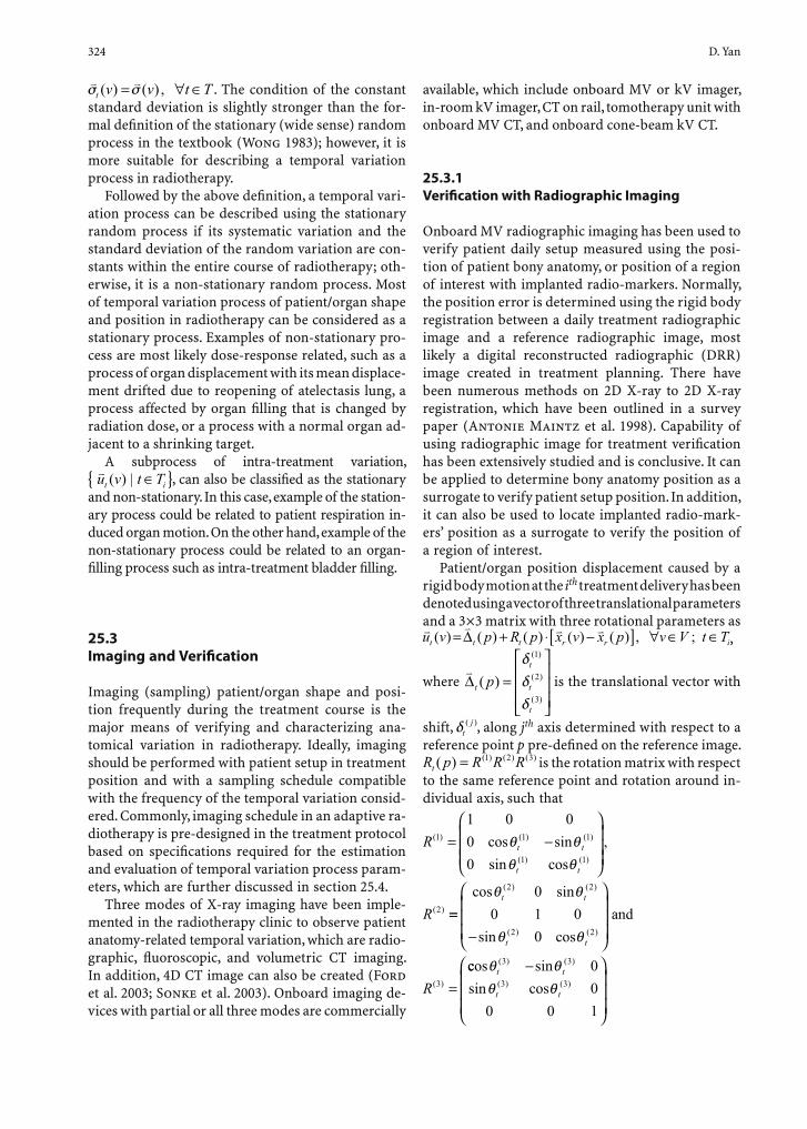
324 D. Yan

v vσ σt v v t T( ) ( ) ,= ∀ ∈ . The condition of the constant standard deviation is slightly stronger than the for-mal defi nition of the stationary (wide sense) random process in the textbook (Wong 1983); however, it is more suitable for describing a temporal variation process in radiotherapy.

Followed by the above defi nition, a temporal vari-ation process can be described using the stationary random process if its systematic variation and the standard deviation of the random variation are con-stants within the entire course of radiotherapy; oth-erwise, it is a non-stationary random process. Most of temporal variation process of patient/organ shape and position in radiotherapy can be considered as a stationary process. Examples of non-stationary pro-cess are most likely dose-response related, such as a process of organ displacement with its mean displace-ment drifted due to reopening of atelectasis lung, a process affected by organ fi lling that is changed by radiation dose, or a process with a normal organ ad-jacent to a shrinking target.

A subprocess of intra-treatment variation, vu v t Tt i( ) | ∈{ }, can also be classifi ed as the stationary

and non-stationary. In this case, example of the station-ary process could be related to patient respiration in-duced organ motion. On the other hand, example of the non-stationary process could be related to an organ-fi lling process such as intra-treatment bladder fi lling.

25.3 Imaging and Verifi cation

Imaging (sampling) patient/organ shape and posi-tion frequently during the treatment course is the major means of verifying and characterizing ana-tomical variation in radiotherapy. Ideally, imaging should be performed with patient setup in treatment position and with a sampling schedule compatible with the frequency of the temporal variation consid-ered. Commonly, imaging schedule in an adaptive ra-diotherapy is pre-designed in the treatment protocol based on specifi cations required for the estimation and evaluation of temporal variation process param-eters, which are further discussed in section 25.4.

Three modes of X-ray imaging have been imple-mented in the radiotherapy clinic to observe patient anatomy-related temporal variation, which are radio-graphic, fl uoroscopic, and volumetric CT imaging. In addition, 4D CT image can also be created (Ford et al. 2003; Sonke et al. 2003). Onboard imaging de-vices with partial or all three modes are commercially

available, which include onboard MV or kV imager, in-room kV imager, CT on rail, tomotherapy unit with onboard MV CT, and onboard cone-beam kV CT.

25.3.1 Verifi cation with Radiographic Imaging

Onboard MV radiographic imaging has been used to verify patient daily setup measured using the posi-tion of patient bony anatomy, or position of a region of interest with implanted radio-markers. Normally, the position error is determined using the rigid body registration between a daily treatment radiographic image and a reference radiographic image, most likely a digital reconstructed radiographic (DRR) image created in treatment planning. There have been numerous methods on 2D X-ray to 2D X-ray registration, which have been outlined in a survey paper (Antonie Maintz et al. 1998). Capability of using radiographic image for treatment verifi cation has been extensively studied and is conclusive. It can be applied to determine bony anatomy position as a surrogate to verify patient setup position. In addition, it can also be used to locate implanted radio-mark-ers’ position as a surrogate to verify the position of a region of interest.

Patient/organ position displacement caused by a rigid body motion at the ith treatment delivery has been denoted using a vector of three translational parameters and a 3¥3 matrix with three rotational parameters asv v v vu v p R p x v x p v V t Tt t t r r i( ) ( ) ( ) ( ) ( ) , ;= + ⋅ −[ ] ∀ ∈ ∈∆ ,

where v∆t

t

t

t

p( )

( )

( )

( )

=⎡

⎣

⎢⎢⎢

⎤

⎦

⎥⎥⎥

δδδ

1

2

3

is the translational vector with

shift, δtj( ), along jth axis determined with respect to a

reference point p pre-defi ned on the reference image. R p R R Rt ( ) ( ) ( ) ( )= 1 2 3 is the rotation matrix with respect to the same reference point and rotation around in-dividual axis, such that

R

R

t t

t t

( ) ( ) ( )

( ) ( )

( )

cos sinsin cos

,1 1 1

1 1

2

1 0 000

= −⎛

⎝

⎜⎜⎜

⎞

⎠

⎟⎟⎟

θ θθ θ

==−

⎛

⎝

⎜⎜⎜

⎞

⎠

⎟⎟⎟

=

cos sin

sin cos

( ) ( )

( ) ( )

( )

θ θ

θ θ

t t

t t

R

2 2

2 2

3

00 1 0

0and

ccos sinsin cos

( ) ( )

( ) ( )

θ θθ θ

t t

t t

3 3

3 3

00

0 0 1

−⎛

⎝

⎜⎜⎜

⎞

⎠

⎟⎟⎟

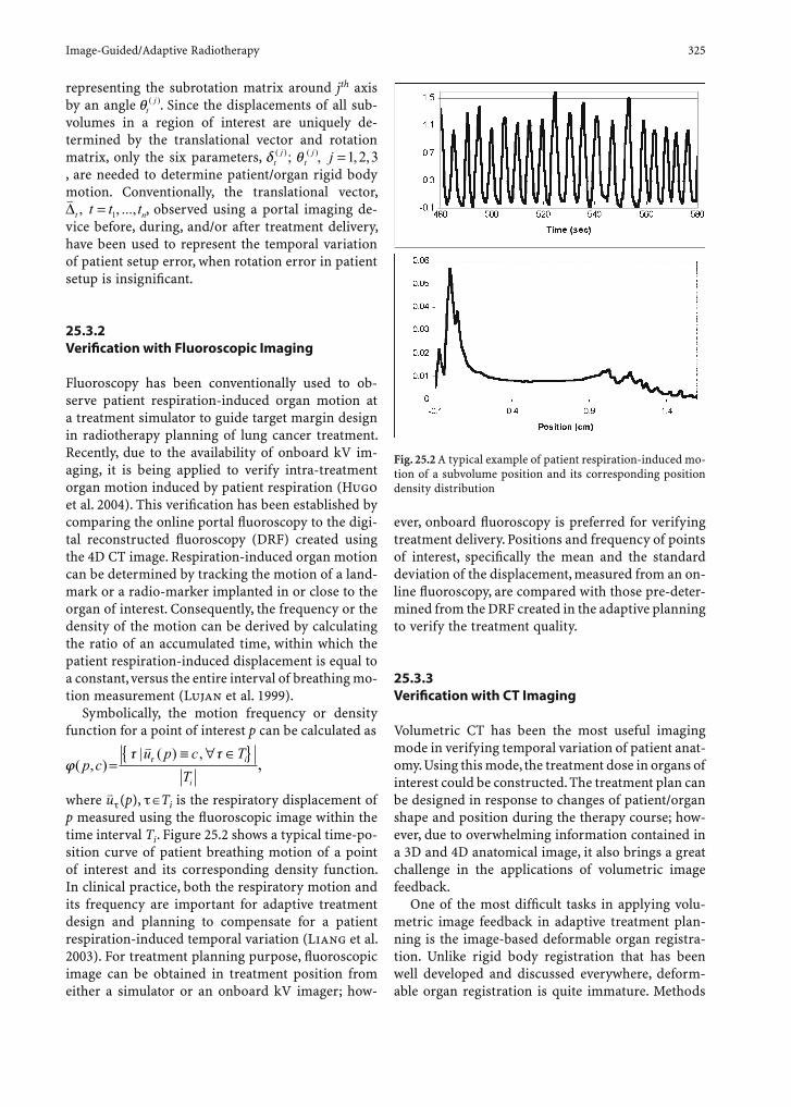
Image-Guided/Adaptive Radiotherapy 325

representing the subrotation matrix around jth axis by an angle θt

j( ). Since the displacements of all sub-volumes in a region of interest are uniquely de-termined by the translational vector and rotation matrix, only the six parameters, δ θt

jt

j j( ) ( ); , , ,=1 2 3, are needed to determine patient/organ rigid body motion. Conventionally, the translational vector, v∆t nt t t, , ...,= 1 , observed using a portal imaging de-vice before, during, and/or after treatment delivery, have been used to represent the temporal variation of patient setup error, when rotation error in patient setup is insignifi cant.

25.3.2 Verifi cation with Fluoroscopic Imaging

Fluoroscopy has been conventionally used to ob-serve patient respiration-induced organ motion at a treatment simulator to guide target margin design in radiotherapy planning of lung cancer treatment. Recently, due to the availability of onboard kV im-aging, it is being applied to verify intra-treatment organ motion induced by patient respiration (Hugo et al. 2004). This verifi cation has been established by comparing the online portal fl uoroscopy to the digi-tal reconstructed fl uoroscopy (DRF) created using the 4D CT image. Respiration-induced organ motion can be determined by tracking the motion of a land-mark or a radio-marker implanted in or close to the organ of interest. Consequently, the frequency or the density of the motion can be derived by calculating the ratio of an accumulated time, within which the patient respiration-induced displacement is equal to a constant, versus the entire interval of breathing mo-tion measurement (Lujan et al. 1999).

Symbolically, the motion frequency or density function for a point of interest p can be calculated as

c T≡ ∀u p{ }ϕ

τ ττ( , )| ( ) ,

p cT

i

i

=∈v

,

where uv

(p), ŒTi is the respiratory displacement of p measured using the fl uoroscopic image within the time interval Ti . Figure 25.2 shows a typical time-po-sition curve of patient breathing motion of a point of interest and its corresponding density function. In clinical practice, both the respiratory motion and its frequency are important for adaptive treatment design and planning to compensate for a patient respiration-induced temporal variation (Liang et al. 2003). For treatment planning purpose, fl uoroscopic image can be obtained in treatment position from either a simulator or an onboard kV imager; how-

ever, onboard fl uoroscopy is preferred for verifying treatment delivery. Positions and frequency of points of interest, specifi cally the mean and the standard deviation of the displacement, measured from an on-line fl uoroscopy, are compared with those pre-deter-mined from the DRF created in the adaptive planning to verify the treatment quality.

25.3.3 Verifi cation with CT Imaging

Volumetric CT has been the most useful imaging mode in verifying temporal variation of patient anat-omy. Using this mode, the treatment dose in organs of interest could be constructed. The treatment plan can be designed in response to changes of patient/organ shape and position during the therapy course; how-ever, due to overwhelming information contained in a 3D and 4D anatomical image, it also brings a great challenge in the applications of volumetric image feedback.

One of the most diffi cult tasks in applying volu-metric image feedback in adaptive treatment plan-ning is the image-based deformable organ registra-tion. Unlike rigid body registration that has been well developed and discussed everywhere, deform-able organ registration is quite immature. Methods

Fig. 25.2 A typical example of patient respiration-induced mo-tion of a subvolume position and its corresponding position density distribution

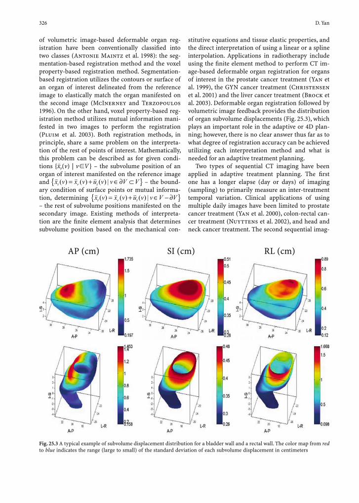
326 D. Yan

of volumetric image-based deformable organ reg-istration have been conventionally classifi ed into two classes (Antonie Maintz et al. 1998): the seg-mentation-based registration method and the voxel property-based registration method. Segmentation-based registration utilizes the contours or surface of an organ of interest delineated from the reference image to elastically match the organ manifested on the second image (McInerney and Terzopoulos 1996). On the other hand, voxel property-based reg-istration method utilizes mutual information mani-fested in two images to perform the registration (Pluim et al. 2003). Both registration methods, in principle, share a same problem on the interpreta-tion of the rest of points of interest. Mathematically, this problem can be described as for given condi-tions {xvr(v) | v V } – the subvolume position of an organ of interest manifested on the reference image and

v v vx v x v u v v V Vt r t( ) ( ) ( ) |= + ∈∂ ⊂{ } – the bound-ary condition of surface points or mutual informa-tion, determining

v v vx v x v u v v V Vt r t( ) ( ) ( ) |= + ∈ −∂{ } – the rest of subvolume positions manifested on the secondary image. Existing methods of interpreta-tion are the fi nite element analysis that determines subvolume position based on the mechanical con-

stitutive equations and tissue elastic properties, and the direct interpretation of using a linear or a spline interpolation. Applications in radiotherapy include using the fi nite element method to perform CT im-age-based deformable organ registration for organs of interest in the prostate cancer treatment (Yan et al. 1999), the GYN cancer treatment (Christensen et al. 2001) and the liver cancer treatment (Brock et al. 2003). Deformable organ registration followed by volumetric image feedback provides the distribution of organ subvolume displacements (Fig. 25.3), which plays an important role in the adaptive or 4D plan-ning; however, there is no clear answer thus far as to what degree of registration accuracy can be achieved utilizing each interpretation method and what is needed for an adaptive treatment planning.

Two types of sequential CT imaging have been applied in adaptive treatment planning. The fi rst one has a longer elapse (day or days) of imaging (sampling) to primarily measure an inter-treatment temporal variation. Clinical applications of using multiple daily images have been limited to prostate cancer treatment (Yan et al. 2000), colon-rectal can-cer treatment (Nuyttens et al. 2002), and head and neck cancer treatment. The second sequential imag-

AP (cm) SI (cm) RL (cm)

Fig. 25.3 A typical example of subvolume displacement distribution for a bladder wall and a rectal wall. The color map from red to blue indicates the range (large to small) of the standard deviation of each subvolume displacement in centimeters

Image-Guided/Adaptive Radiotherapy 327

ing has been aimed to detect organ motion induced by patient respiration. These images, which manifest organs of interest at different breathing phases, can be obtained from a respiratory correlated CT imag-ing (Ford et al. 2003) or a slow rotating cone-beam CT (Sonke et al. 2003). Clinical application of this measurement has been focused on lung cancer treat-ment; however, it has no limit to be extended to the other cancer treatment where patient respiration ef-fect is signifi cant, such as liver cancer treatment. In principle, both types of sequential imaging are 4D CT imaging, although the terminology of 4D CT im-aging has been specifi cally used to describe the 3D sequential CT images induced by patient respiration. Commonly, either an onboard or an off-board volu-metric imager can be applied to measure patient or-gan motion for the purpose of offl ine planning modi-fi cation; however, onboard imaging is a favorable tool for both online and offl ine treatment planning modi-fi cation and adjustment.

25.4 Estimation and Evaluation

It has been discussed that temporal variation of patient/organ shape and position during the whole treatment course could be modeled as a random process of organ subvolume displacement, denoted

as v

Uu v t T T v Vt ii

n

( ) | ,∈ ⊂⎧⎨⎩

⎫⎬⎭

∀ ∈=1

, or multiple

subprocesses during each treatment delivery, denoted as v V{ }vu v t T i nt i( ) | , ; ,...,∈ ∀ ∈ =1 . The former has been primarily considered in the design of offl ine imaging and planning modifi cation as indicated as the outer loop of the adaptive system in Fig. 25.1; the latter, on the other hand, has to be considered additionally in the design of online image-guided adjustment – the inner loop of Fig. 25.1. Although process parameter estimation and treatment evalu-ation are normally performed in the outer feedback loop, they will be utilized to modify and update the planning and adjustment parameters for both offl ine and online planning modifi cation and adjustment.

As has been discussed in section 25.2, the key parameters of a temporal variation process are the systematic variation and the standard deviation of random variation of subvolume displacement [see also Eq. (4)]. These parameters, therefore, have to be estimated for either offl ine or online mechanisms. Moreover, the cumulative dose/volume relationship

of organs of interest and the corresponding biologi-cal indexes can also be estimated and evaluated. In addition, effects of dose per fraction on a critical nor-mal organ should also be considered in the cumula-tive dose evaluation when online image guided hypo-fractionation is implemented, because the effect of temporal variation of organ fraction dose can be sig-nifi cantly enlarged in a hypo-fractionated treatment (Yan and Lockman 2001).

Multiple imaging (or sampling) performed in the early part of treatment has been the common means to estimate the mean µt

v (the systematic variation)

and the standard deviation σtv

(the characteristic of the random variation) of a temporal variation pro-cess. Estimation can be performed once using mul-tiple images obtained early in treatment course, in batches, or continuously. In general, imaging sched-ule in an adaptive radiotherapy system has been selected in a treatment protocol based on a pre-de-signed strategy of adaptive treatment. In case of the single offl ine adjustment of patient position during the treatment course, optimal sampling schedule of four to fi ve observations obtained daily in the early treatment course has been suggested (Yan et al. 2000) and proved to be a favorable selection with respect to the criteria of minimal cumulative displacement (Bortfeld et al. 2002); however, so far, there has not been any systematic study to explore the relationship between the imaging schedule and the treatment dose/volume factor. A preliminary study (Birkner et al. 2003) demonstrated that there was only a mar-ginal improvement for prostate cancer IMRT, when offl ine-planning modifi cation is continuously per-formed compared with a single modifi cation after fi ve measurements. Parameter estimation for a given temporal variation process could be straightforward. Example of such process is the organ motion induced by patient respiration. In this case, the motion can be characterized using 4D CT imaging and fl uoroscopy before the treatment if the process is stationary; oth-erwise, the estimation can be performed multiple times during the treatment course.

25.4.1 Parameter Estimation for a Stationary Temporal Variation Process

Without loss of generality, let | ;u t ∈ ={ }v T i kt ii, ...,1

be the measurements (the sample size k is commonly small except for the respiratory motion) of subvol-ume displacement for an organ of interest obtained from k CT image measurements, or displacement of

328 D. Yan

a reference point when radiographic images or fl uo-roscopy are used for the measurements. The stan-dard unbiased estimations of the constant mean, µv, and the constant standard deviation, σv, based on the measurements are

ˆ ˆ ˆ1 1v vv vµ σ= =∑ ∑ ui i

v; ( )µ−

−= =11 1

2

ku

kti

k

ti

k

.

In addition, the potential residuals between the true and the estimation can also be evaluated based on the standard confi dence interval estimation as

α ,2 1 ⋅ ≤− −

µ µ1 1

v vv

v v;/,

σ σχ

σα

− ≤ − ⋅−tk

kk

k2

1ˆ ˆ ,

where the factor t 2 1−/ ,α k has the t-distribution with k-1 degrees of freedom and 1 1− −χ α

2, k has the

χ 2 −distribution with k-1 degrees of freedom, and both them have the confi dence 1-α.

The other method of estimating the systematic variation is the Wiener fi ltering (Wiener 1949). Applying the Wiener fi ltering theory, the optimal es-timation of the systematic variation is constructed by minimizing the expectation of the estimation and the truth, such as

v vµ µMin E u ut tk( ) | , ..., , ,v v v v

µ σ−⎡⎣ ⎤⎦2

1Σ Μˆ ,

with conditions of the k measurements, the standard deviation of the individual systematic variations,

0 0

0 0

vvΣµ

µ

µ

µ

σ

σ

σ

=

⎛

⎝

⎜⎜⎜⎜

⎞

⎠

⎟⎟⎟⎟

1

2

3

0 0

,

and the root-mean-square of the individual standard deviations of the random variations,

0 0

0 0v

vΜσ

σ

σ

σ

µ

µ

µ

=

⎛

⎝

⎜⎜⎜⎜

⎞

⎠

⎟⎟⎟⎟

1

2

3

0 0

.

Consequently, the estimation of the systematic varia-tion is

( )k k= ⋅u c Σ Σv v v v vv v v,µ µ µ σ= ⋅ ⋅ ⋅ +

=

−∑ck t

i

k

i

11

1Μˆ .

It has been proved that for a temporal variation process, Σ

vvµ and

vvσΜ could have similar values; there-

fore, the Wiener estimation can be simplifi ed as

v vµ =+

⋅=∑1

1 1kut

i

k

iˆ .

In addition to the mean and the standard devia-tion, knowledge of the probability density v ( )ϕ of each subvolume displacement in a temporal varia-tion process could also be useful; however, except for patient respiratory motion that can be determined

directly using 4D CT and fl uoroscopy (as described in section 25.3.2), the majority of temporal variations can only be practically measured a few times, and us-ing these small numbers of measurements to estimate a probability distribution is most unlikely possible. Therefore, pre-assumed normal distribution has been applied in the clinic. It has been demonstrated that the actual treatment dose in an organ subvolume is most likely determined by its systematic variation and the standard deviation of its random variation. The actual shape of the displacement distribution is less important (Yan and Lockman 2001); there-fore, the pre-assumption of the normal distribution,

ˆ( )v N µ σv vˆ ( )ϕ ( ), ( )v v= 2ˆ , is acceptable in the treatment dose estimation.

Parameter estimation of stationary temporal variation process can be applied for both offl ine and online feedback. Examples of offl ine feedback in-clude using multiple radiographic portal imaging to characterize patient setup variation, multiple CT im-aging to characterize internal organ motion, and 4D CT/fl uoroscopy imaging to characterize respiratory organ motion. Application for online feedback is cur-rently limited to characterize intra-treatment organ motion assessed by multiple portal imaging and por-tal fl uoroscopy. For the online CT image-guided pros-tate treatment, parameter estimation for intra-treat-ment variation also depends on patient anatomical conditions. There has been a study (Ghilezan et al. 2003) that showed that the intra-treatment variation of prostate position was primarily controlled by the rectal fi lling conditions.

25.4.2 Parameter Estimation for a Non-stationary Temporal Variation Process

Parameters to be estimated in a non-stationary process are similar to those in a stationary process; however, instead of constants, they can be piecewise constants, such as respiration-induced organ motion during lung cancer treatment, or a continuous func-tion of time, such as bladder-fi lling-induced motion during treatment delivery. It is relatively simple to es-timate the process parameters that are piecewise con-stants. The estimation in each constant period will be performed as same as the one for a stationary process; however, the estimation for a process with parameter as a continue function will be less straightforward. The most common method to estimate a function based on fi nite number of samples is the least-squares estimation. With pre-selected orthogonal base of functions t t1 2φ φ

vφ φ( ) ( ) ( ) ( )( ) ( ) ( ) ( )j j j

mjt t= ⋅⋅⋅⎡⎣ ⎤⎦, i.e.

Image-Guided/Adaptive Radiotherapy 329

= =φij it t i m( ) ( ) , , ,...,−1 1 2 , the estimations for both

the systematic variation and the standard deviation of the random variation are

ˆˆµ

σµ φa t ( )= ⋅ ( );( )

( ) ( ) ( )

( ) ( )

tj

ij

ij

tj

tj

tj

i

k

i

m u

k m

i i

=−

−=

=

∑ 2

1

1∑∑

=

,

, , ,j 1 2 3 where

ˆ

a

a

u

u

j

mj

T T

tj

tj

k

11

1( )

( )

( )

( )

;� �

⎡

⎣

⎢⎢⎢

⎤

⎦

⎥⎥⎥= ⋅( ) ⋅ ⋅

⎡

⎣

⎢⎢⎢

⎤

⎦

⎥⎥⎥

−Φ Φ Φ ΦΦ =

⎡

⎣

⎢⎢⎢

⎤

⎦

⎥⎥⎥

v

�v

φ

φ

( )

( )

( )

( )

j

jk

t

t

1

.

As the extension of the Wiener fi lter, the Kalman fi lter has also been applied to estimate the system-atic variation for a non-stationary process assuming that the systematic variation is a linear function of time (Yan et al. 1995; Lof et al. 1998; Keller et al. 2004). In addition, similar to the description in the previous section, the probability density of each subvolume displacement can be estimated as ˆt v( )ϕ for a respiratory motion or a normal distribution

ˆ ˆµ σv v( )t tv N( ) ( ), ( )ϕ tv v= 2ˆ .Applications of parameter estimation for a non-

stationary process have been few. One study (Ford et al. 2002) attempted to determine the reproduc-ibility of patient breathing-induced organ motion. It revealed that the mean of patient respiration-in-duced organ motion could considerably vary during the course of NSCLC due to treatment and patient related factors; therefore, multiple measurements of 4D CT and fl uoroscopy, i.e., once a week, may be nec-essary to manage adaptive treatment of lung cancer. Regarding parameter estimation for a continuous function, one study (Heidi et al. 2004) has been per-formed to estimate bladder expansion and potential standard deviation for the online image-guided blad-der cancer treatment, where bladder subvolume posi-tion was modeled as a linear function of time.

25.4.3 Estimation of Cumulative Dose

Including temporal variation in cumulative dose estimation can be performed using the knowledge of subvolume displacement distribution. At pres-ent, the construction is performed assuming time invariant spatial dose distribution calculated from the treatment planning. It implies that the dose dis-tribution remains constant spatially regardless the changes of patient anatomy; however, this assump-tion can only be acceptable if spatial dose variation

induced by the changes of patient body shape and tissue density is insignifi cant, i.e., during the pros-tate cancer treatment; otherwise, the dose has to be recalculated using each new feedback image. Of course, this can only be performed when CT image feedback is applied.

Cumulative dose for each subvolume in the organ of interest can be evaluated as

or

with considering the biologi-cal effect of dose per fraction, where ds is the standard fraction dose 1.8 or 2 Gy. This dose expression is a very general and can be simplifi ed based on the at-tributes of a temporal variation.

For a stationary process with the time invariance dose distribution, the cumulative dose in an organ of interest can be estimated directly utilizing the prob-ability density of subvolume displacement �^ (v) and the planned dose distribution dp as

(5)

if the planned dose per treatment fraction is fi xed. When an offl ine planning modifi cation is performed at the k+1 treatment delivery, based on the previous k image measurements, then the cumulative dose can be estimated by considering the treatments which have been delivered (Birkner et al. 2003), such that

.

The estimation can also be performed using the mean and the standard deviation of a temporal varia-tion (Yan and Lockman 2001), such that

(6)

where is the mean dose gradient in the interval , and is the dose curvature at point .

Equation (6) provides a very important structure on the parameter design of adaptive planning and ad-justment (discussed in the next section).

Using the estimated dose, radiotherapy dose re-sponse parameters, such as the EUD, NTCP, and TCP, can be evaluated using the common methods that have been discussed elsewhere.

330 D. Yan

25.5 Design of Adaptive Planning and Adjustment

Design of adaptive planning and adjustment con-tains computation and rules to select planning and adjustment parameters, and to update the schedule of imaging, delivery, and adjustment. Ideally, imag-ing/verifi cation, estimation/evaluation, and plan-ning/adjustment should be performed with the identical sampling rates, and the planning/adjust-ment parameters should be selected in such way that the adaptive radiotherapy system can be completely optimized; however, this is most unlikely possible when clinical practice is considered. Only a few pos-sibilities have been investigated and are discussed here.

25.5.1 Design Objectives

Objectives in the design of adaptive planning/ad-justment are commonly specifi ed in an adaptive treatment protocol. The objectives are (a) to im-prove treatment accuracy by reducing the system-atic variation, (b) to reduce the treated volume and improve dose distribution by reducing the system-atic variation and compensating for patient specifi c random variation, (c) to reduce the treated volume and improve dose distribution by reducing the both systematic and random variations, and (d) to ad-ditionally improve treatment effi cacy by alternating daily dose per fraction and number of fractions. Clearly, an objective has to be selected based on expected treatment goals and available technolo-gies. The fi rst two can be implemented using an offl ine feedback technique. Conversely, online image guided adjustment or planning modifi cation has to be implemented to achieve the objectives (c) or (d). Most of offl ine techniques have implemented the re-planning and adjustment once during the treatment course, except for the case when a large residual ap-peared in the estimation. On the other hand, most of online techniques have aimed to adjust patient treatment position only by moving the couch and/or beam aperture; therefore, it is also important to implement a hybrid technique, where offl ine plan-ning is performed to modify the ongoing treatment plan in certain time intervals (e.g., weekly) during online daily adjustment process.

25.5.2 Adaptive Planning and Adjustment Parameters

Given organs of interest, the target and surrounding critical normal structures, the aim of an adaptive treatment planning is to design and modify treat-ment dose distribution in response to the tempo-ral variations observed in the previous treatments. Considering the dose expressed in Eq. (6), four fac-tors play the key roles on treatment quality and can be considered in the adaptive treatment planning and adjustment design; these are two patient/organ-geometry related factors, the systematic variation µv and the standard deviation of the random variation σv for each subvolume in the organs of interest, and two patient dose-distribution-related factors, the dose

gradient dt and the dose curvature ∂∂

2

2

dx

tv at each

spatial point in the region of interest. Theoretically, any treatment planning and adjustment parameter, which can control these factors, can be selected to modify and improve the treatment.Planning and adjustment parameters can be divided into two classes: one contains patient-positioning pa-rameters, such as couch position and rotation, beam angle, and collimator angle, which can be applied to reduce both the systematic and random variations {µv, σv}; however, these parameters can only adjust variations induced by rigid body motion and im-prove position accuracy and precision, but have lim-its to manage variations induced by organ deforma-tion and cannot improve treatment plan qualities; the other contains dose-modifying parameters, such as target margin, beam aperture, beam weight, and beamlet intensities. These parameters are typically used to adjust dose distribution, thus modifying

∇ ∂∂

⎧⎨⎩

⎫⎬⎭

d dxt

t,2

2v in the region of interest to improve

ongoing treatment qualities. In addition, prescription dose, dose per fraction, and number of fractions have also been used as parameters for adaptive planning (Yan 2000).

25.5.3 Adaptive Planning and Adjustment Parameter and Schedule: Selection and Modifi cation

In an ideal adaptive radiotherapy system, design of planning and adjustment should have a function of automatically selecting on going planning/adjust-

Image-Guided/Adaptive Radiotherapy 331

ment parameters and schedules of imaging, delivery, and adjustment; thus, a new treatment plan can be calculated by including the observed temporal varia-tions and estimation, optimized using the selected parameters and executed with the new schedules. In principle, a set of pre-specifi ed rules and control laws could be used in the design, which match the param-eters of temporal variation process to the parameters and schedules of adaptive planning and adjustment.

Basic rules can be created utilizing the discrep-ancies between the ideal treatment under the ideal condition (i.e., no temporal variation occurs) and the “actual” treatment that includes the temporal varia-tions. The discrepancies can be either the organ vol-ume/dose discrepancy, or the discrepancies of EUD, TCP, and/or NTCP determined from the planned dose, ∈ ={ }v V| ,D v i li( ) ,...,1 , in organs of interest, Vi , calculated without considering temporal varia-tions vs those determined from the estimated dose distribution ˆ v V∈ ={ }( ) | , ,...,D v i li 1 constructed from a treatment plan created using pre-specifi ed planning/adjustment parameters and including the estimation of temporal variations. A set of pre-defi ned tolerances V D{ }δ δ δ δ δEUD TCP NTCP, , , , is then used to test whether or not the discrepancies,

∆ ∆≤ ≤δ δV D EUDD V EUD( ) , ,≤δ ∆ ≤δTCP TCP , and/or∆ ≤δNTCP NTCP, hold within the predefi ned ranges. In addition, these tolerances can also be utilized to eval-uate and rank the potential treatment quality with respect to different groups of planning/adjustment parameters and adjustment methodology (offl ine or online). Depended on the variation type (rigid or non-rigid) and the objectives of planning/adjust-ment, the planning and adjustment parameters could be selected as (a) couch position/rotation, beam an-gle, and/or collimator angle (online or offl ine posi-tion adjustment for a rigid body motion), (b) target margin, beam aperture, beam weight (intensities), and/or prescription dose (online or offl ine planning modifi cation), and (c) beamlet intensity, prescription dose, and/or dose per fraction plus number of frac-tions (online planning modifi cation). Contrarily, a subset of patients, who have insignifi cant temporal variation, can also be identifi ed; therefore, no re-plan-ning and adjustment are necessary for this subset.

There have been limited studies on utilizing con-trol laws to automatically modify the planning and adjustment parameters. A decision rule (Bel et al. 1993) has been proposed and applied for the offl ine adjustment of systematic variation induced by daily patient setup. This decision rule is constructed by assuming the statistical knowledge of patient setup variation, and automatically schedules the setup ad-

justment based on the estimated systematic variation, and pre-designed “action levels.” The other method to control the offl ine planning and adjustment has been “no action level” but including estimated resid-uals in the target margin design, and primarily single modifi cation after four to fi ve consecutive observa-tions (Yan et al. 2000; Birkner et al. 2003). An early investigation (Lof et al. 1998) on the adaptive plan-ning has modeled the cumulative dose and beamlet intensities (control parameters) recursively using a linear system, and created a quadratic objective from the prescribed doses and the estimated doses. Based on the optimal control theory (Bryson and Ho 1975), the intensity fl uence adjustment therefore follows a standard linear feedback law – a linear function of the dose discrepancy in organs of interest. Intuitively, the beamlet intensities in the treatment should be ad-justed proportionally to the estimated dose discrep-ancy. Similar methodology has been also proposed for adaptive optimization using the tomotherapy delivery machine (Wu et al. 2002). In addition to beam intensity fl uence, a control law has also been proposed to manipulate the prescription dose per treatment fraction and the total number of treatment fractions in an online image-guided process (Yan 2000). This control law utilizes temporal variation of dose/volume of critical normal organs to select the most effective dose of the fraction and the total num-ber of fractions.

Most problems in adaptive radiotherapy are easily described but hardly solved. Compared with a direct 4D inverse planning after k number of observations, control laws derived from an ideal system model commonly provide only limited roles in the clinical implementation. For the clinical practice, most tem-poral variations of patient/organ shape and position can be described using stationary random processes, and therefore the control mechanism is straightfor-ward. Applying one or few planning modifi cations, the systematic variation can be maximally eliminated and thus patient treatment can be signifi cantly im-proved in an offl ine adjustment process. Residuals are commonly inverse proportional to the frequency of the verifi cation, estimation, and adjustment. These residuals could be signifi cantly large to diminish the anticipated gain of adaptive treatment for certain patients; therefore, a decision rule should be applied to modify the schedule of imaging and adjustment if these patients are identifi ed during the treatment course.

Sampling rates of imaging/verifi cation, estima-tion/evaluation, and adaptive planning/adjustment should be scheduled to match the rate of the aimed

332 D. Yan

temporal variations. Mismatch results in signifi cant downgrading of the expected treatment quality; therefore, before selecting objectives in an adaptive treatment design, specifi cally for an online adjust-ment process, one should ensure that appropriate sampling rates of imaging/verifi cation, estimation/evaluation, and adaptive planning/adjustment could be implemented.

25.6 Adaptive Planning and Adjustment

Adaptive planning and adjustment are implemented with the pre-design parameters. The adaptive plan-ning is often performed including the temporal varia-tions in the planning dose calculation; therefore, it has also been called “4D treatment planning.” There have been two methods to perform a 4D planning. The fi rst (indirect method) does not directly include the temporal variation in the planning dose calcula-tion. Instead, it constructs the PTV and margins of organs at risk based on the characteristics of patient specifi c temporal variations and a generic planned dose distribution, and then performs a conventional conformal or inverse planning accordingly. The sec-ond (direct method) performs treatment planning by directly including the temporal variations in the dose calculation as has been discussed in section 25.4.3. The adaptive treatment plan designed with the ex-pected dose distribution can best compensate for the temporal variations. Consequently, pre-designed target margin is either unnecessary or used only to compensate for the residuals of the estimation.

25.6.1 Indirect Method

Planning technique in the indirect method is pri-marily the same as the conventional one except for the defi nition of the planning target volume and the margins of organs at risk. For a rigid body motion without signifi cant rotation, the patient specifi c tar-get margin in each direction j after k observations can be constructed by considering the residuals of the estimations of the systematic and random variations (Yan et al. 2000), such that

1 1

m c tk

c kjj ,k

j

jk

j( )/

( )

,

( )( )= ⋅ + ⋅ − ⋅−− −

2 1 2

1σχ

σα

ˆ ˆα ,

where t ,k/ −2 1α and 1 1k,− −2χ α have been defi ned in sec-

tion 25.4.1. The factor cj is determined by ensuring that the potential dose reduction in the target with the corresponding margin is less than a pre-defi ned dose tolerance δ , such that

ˆ ⋅ ≤ϕ ξ⋅ )( )( )− +

( )= ⋅ ξ δ∆D c n

d x

d x m cj

p rj

p rj j j

j

j( )( )

(( )

( ) ( )

( )

−

⎡

⎣⎢⎢

⎤

⎦⎥⎥ξ

( )

−∞

∞

∫ d j ,

where d x( )p rj( ) is the planning dose around the

CTV edge xrj( ) on the j axis. ϕ ξ )j( ( ) is the estimated

probability distribution with the mean tk,k

j

/

( )

2 1− ⋅σ

αˆ

(the residual of the systematic variation) and the

standard deviation 1 1

k

k

j− ⋅− −

12χ

σα ,

( )ˆ .

It is clear that the calculation of dose discrepancy here is approximated assuming the spatial invari-ance of planning dose distribution. In addition, this evaluation can also be approximated using the dose gradient and curvature around the CTV edge as in-dicated by Eq. (6), such that

τ π

j

2 1

; (( )σ

≈ ⋅∆D c n

tk

dxdx

jj

,k pj

jp

j

( )

[ , ]

( )

( )

/( )

( )

( )

⋅⋅∂∂

+ ⋅∂∂

−

σ

σ π2

2 222 1

⎛

⎝

⎜⎜⎜⎜

⎞

⎠

⎟⎟⎟⎟

= − = − + ⋅−τ πx m c x m c trj j

j rj j

,k( ) ( ) ( ) ( )

/( ) ) σ

δ

j

k

≤

ˆ

ˆˆ

α

α

.

This method can be further extended to construct CTV-to-PTV margin that compensates for much broad type of variations including organ deformation. Let CTV∂ represent the boundary of CTV, then the 3D margin can be constructed using the vector normal to target surface at each boundary point ∈v CTV∂ , such that

σvv

vm c v t vk

c k v,kk

( , ) ( ) ( )/,

= ⋅ + ⋅ − ⋅−− −

2 11 12

1χ

σα

α

ˆ ˆ .

Similarly, the c is determined such that the following inequality

( ) ϕ ξ ξ

∆D c v

d x v

d x v v m c vp r

p r

( , )

( )

( ) ( ) ( , )(

=

( )− + −

⎡

⎣⎢⎢

⎤

⎦⎥⎥⋅

v

v v vv

ξδ) ⋅ ≤∫ d

R

v3

ˆ⋅n

Image-Guided/Adaptive Radiotherapy 333

holds; therefore, the patient-specifi c PTV can be formed by creating a new surface with the vectors vm c v v CTV( , ),∀ ∈ ∂ .

Typical adaptive planning/adjustment with us-ing the indirect method includes (a) using imaging measurements to perform the estimation, (b) adjust-ing patient position or beam aperture to correct the estimated systematic variation, (c) constructing a patient specifi c PTV, and (d) performing a conven-tional treatment planning or inverse planning. Since patient-specifi c PTV construction is also dependent on the planning dose distribution, primarily the dose gradient and curvature around the neighborhood of the CTV edge, control parameters, which can directly adjust the dose gradient and curvature, are important for the adaptive treatment planning.

25.6.2 Direct Method

In the direct method of 4D planning, temporal varia-tions are directly included in the planning dose calcu-lation. Consequently, dose distribution in the neigh-borhood of each subvolume of organs of interest can be designed by selecting beam aperture or modu-lating beam intensity fl uence to effectively compen-sate for the systematic and the random variations estimated from previous observations; therefore, pa-rameters of temporal variation and dose distribution are automatically included in the treatment planning optimization. However, because the position of each subvolume in a 4D planning is a distribution function rather than static, it considerably increases the time and complicity of the dose calculation.

Most 4D adaptive planning have been completed using an inverse planning engine that searches the optimal beam intensity fl uence based on the objec-tive function calculated using the estimated dose dis-cussed in section 25.4.3. Objective function and search algorithm commonly remain the same as those in the conventional inverse planning, but dose computation or estimation is much time-consuming, specifi cally when including feedback volumetric CT images in the computation becomes necessary. Some simpli-fi cations on dose computation have been applied to reduce the calculation time. One study (Birkner et al. 2003) has directly included the samples of organ subvolume displacement in the dose estimation dur-ing the inverse planning iteration, such that for each subvolume, v, the expected dose after k treatment de-livery is computed as

v w( )⋅ +

( , ) ( ) ( )

( ) ( ) ( ),

D v d x v n kk

d x v u v

tt

k

t

r i ji

Φ

Φ

= ( )+ −

+

=∑

12

v

v v v

,, j

k

=∑

1

ˆ (7)

where ujv ( )v is the sample of subvolume displace-

ment induced by internal organ motion, and wjv ( )v

is the sample of subvolume displacement induced from patient setup. is the beam-intensity map to be optimized. It has been demonstrated that the op-timization result converges after fi ve observations in an offl ine adaptive process for prostate cancer radio-therapy. Figure 25.4 shows a typical dose distribution from the 4D inverse planning, where the dose gradi-ent and curvature in the adjacent region between target and normal structure were designed to best compensate for the variations induced from treat-ment setup and internal organ motion.

The fundamental difference between the 4D plan-ning in an offl ine process and the one in an online process is the dose construction in the objective func-tion. Offl ine 4D planning aims to optimize treatment plan for all remaining treatment. Meanwhile, online

Fig. 25.4 Dose distribution (colored isodose lines) calculated from a 4D inverse planning of prostate cancer superimposed on the organ occupancy density (gray area)

334 D. Yan

4D planning aims to optimize treatment plan for the current treatment; however, both need to include pre-vious measurements in the dose construction. On the other hand, in addition to beam aperture, intensity fl uence and prescription dose, extra planning pa-rameters, such as dose per fraction and number of fractions, can also be considered in an online process. In this case, a treatment planning is performed be-fore each treatment delivery by including all previ-ous observations to optimize the intensity map and prescription dose for the current fraction, as well as estimating the total number of fractions (Yan 2000). Before the kth treatment delivery, the cumulative dose in the online treatment planning is constructed in-cluding the previous k-1 treatment deliveries as

Φ =, , ˆd n)⎜⎜n

( )( )( ,

( )( )

D vk

d x vd x v

d

d xk

tt

k

tt t

s

k

( )⋅ + ( )+

+

=

−

∑1

1 vv

v

βα

βα

kkk k

s

vd x v

d( ),

( ),Φ

Φ⋅

++

⎛

⎝

⎜⎜⎜

⎞

⎠

⎟⎟⎟⎟⎟

βα

βα

vˆˆ (8)

where planning parameters, , ,{ }Φd nk ˆ , are the beam intensity map, the prescription dose for the k frac-tion, and the number of fractions.

25.7 Adaptive Treatment Protocol

Clinical protocol of adaptive treatment provides a structure and work fl ow of the image feedback and adaptive planning system. As indicated in Fig. 25.1, schedules of imaging, delivery, and planning/adjust-ment for the patient treatment are pre-defi ned in a protocol based on the feedback mechanism, of-fl ine or online, and nature of the temporal variation process (stationary or non-stationary). In addition, these schedules can be updated based on the feed-back observations. At present, study on the schedule optimization has been limited.

There could be many selections of adaptive control mechanisms for a given treatment site and desired treatment objectives. Two examples, which have be-ing currently implemented in a radiotherapy clinic, are outlined here. Instead of describing the whole protocol, procedures that directly link to the techni-cal aspects of the adaptive treatment are described, which include the structures of imaging/verifi cation, estimation/evaluation, parameter design and adap-tive planning/adjustment.

25.7.1 Example 1: Image-Guided/Adaptive Radiotherapy for Prostate Cancer

Pre-treatment plan with respect to four-fi eld box technique or inverse planning is designed to deliver daily fraction dose of 3.9 Gy to target isocenter for total 15 fractions. The feedback loops include an on-line CT image guided adjustment, and an offl ine CT image-guided planning modifi cation.

Inner feedback loop (online) in the adaptive RT sys-tem (Fig. 25.1)1. Imaging/verifi cation: CT imaging acquired using

an onboard kV cone-beam device before treat-ment delivery for patient at the treatment position. Simulating couch motion and collimator rotation to align a template of target outline pre-defi ned on the reference image to the target manifested on the online image. Compare the motions against to the pre-defi ned tolerances

2. Adjustment: adjusting couch position and colli-mator rotation accordingly, if necessary

Outer feedback loop (offl ine) in the adaptive RT sys-tem (Fig. 25.1)1. Imaging/verifi cation:

after each fi ve treatment deliveries, performing deformable organ registration for the daily CT images

2. Estimation/evaluation: estimating the parameters of temporal variation, and the cumulative dose for organs of interest

3. Design of planning/adjustment: If ≤ ≤δ δ∆ ∆CTV D D V( %) %ˆ due to target shape change, and/or if the shape and position of organs at risk change signifi cantly, arranging a 4D plan-ning with planning parameter of beam aperture or beam intensity fl uence

4. Adaptive planning/adjustment: performing the 4D planning and adjusting the on-going treatment accordingly

25.7.2 Example 2: Image-Guided/Adaptive Radiotherapy for NSCLC

Pre-treatment planning is performed with respect to the target (GTV) at the mean respiratory position determined using a 4D CT image and fl uoroscopy. A patient-specifi c PTV is constructed using the indirect

Image-Guided/Adaptive Radiotherapy 335

method discussed in section 25.6.1. The treatment plan is designed to deliver daily dose of 3.0 Gy (bid) to the minimum of PTV dose for total 47 fractions. The feedback loops include online fl uoroscopy-guided adjustment and offl ine 4D CT image-guided planning modifi cation.

Inner feedback loop (online) in the adaptive RT sys-tem (Fig. 25.1)1. Imaging/verifi cation: fl uoroscopic imaging

acquired using an onboard kV cone-beam device before treatment delivery for patient at the treat-ment position

2. Identify the mean respiratory position for a region or point of interest, and compare it with that pre-determined at the treatment planning with respect to a pre-defi ned tolerance

3. Adjustment: adjusting couch position accordingly, if necessary

Outer feedback loop (offl ine) in the adaptive RT sys-tem (Fig. 25.1)1. Estimation/evaluation: determine the standard

deviation of the respiratory motion measured from the daily fl uoroscopy

2. Design of planning/adjustment: if the standard deviation is larger, with respect to a pre-defi ned tolerance, than the one determined in the pre-planning, acquire a new 4D CT image and perform a new 4D planning

3. Adaptive planning/adjustment: performing the 4D planning and adjustment accordingly

25.8 Summary

Adaptive radiotherapy system is designed to system-atically manage treatment feedback, planning, and adjustment in response to temporal variations oc-curring during the radiotherapy course. A temporal variation process, as well as its subprocess, can be classifi ed as a stationary random process or a non-stationary random process. Image feedback is nor-mally designed based on this classifi cation, and the imaging mode can be selected as radiographic imag-ing, fl uoroscopic imaging, and/or 3D/4D CT imaging, with regard to the feature and frequency of a patient anatomical variation, such as rigid body motion and/or organ deformation induced by treatment setup, or-gan fi lling, patient respiration, and/or dose response. Parameters of a temporal variation process, as well as

treatment dose in organs of interest, can be estimated using image observations. The estimations are then used to select the planning/adjustment parameters and the schedules of imaging, delivery, and plan-ning/adjustment. Based on the selected parameters and schedules, 4D adaptive planning/adjustment are performed accordingly.

Adaptive radiotherapy represents a new standard of radiotherapy, where a “pre-designed adaptive treatment strategy” a priori treatment delivery will replace the “pre-designed treatment plan” by consid-ering the effi ciency, optima, and also clinical practice and cost.

Acknowledgements

The work presented in this chapter was supported in part by NCI grants CA71785 and CA091020.

References

Antonie Maintz JB, Viergever MA (1998) Medical image analy-sis, vol 2. Oxford University Press, Oxford, pp 1–38

Astrom KJ, Wittenmark B (1995) Adaptive control, 2nd edn. Addison-Wesley, Reading, Massachusetts

Bel A et al. (1993) A verifi cation procedure to improve patient setup accuracy using portal images. Radiat Oncol 29:253–260

Birkner M et al. (2003) Adapting inverse planning to patient and organ geometrical variation: algorithm and implemen-tation. Med Phys 30:2822–2831

Bortfeld T et al. (2002) When should systematic patient posi-tioning errors in radiotherapy be corrected? Phys Med Biol 47:N297–N302

Brierley JD et al. (1994) The variation of small bowel volume within the pelvis before and during adjuvant radiation for rectal cancer. Radiother Oncol 31:110–116

Brock KK et al. (2003) Inclusion of organ deformation in dose calculations. Med Phys 30:290–295

Bryson AE Jr, Ho YC (1975) Applied optimal control. Hemi-sphere Publishing Corporation, Washington, DC

Christensen GE et al. (2001) Image-based dose planning of intracavitary brachytherapy registration of serial-imaging studies using deformable anatomic templates. Int J Radiat Oncol Biol Phys 51:227–243

Davies SC et al. (1994) Ultrasound quantitation of respiratory organ motion in the upper abdomen. Br J Radiol 67:1096–1102

Ford EC et al. (2002) Evaluation of respiratory movement during gated radiotherapy using fi lm and electronic portal imaging. Int J Radiat Oncol Biol Phys 52:522–531

Ford EC et al. (2003) Respiration-correlated spiral CT: a method of measuring respiratory-induced anatomic motion for radiation treatment. Med Phys 30:88–97

Ghilezan M et al. (2003) Prostate gland motion assessed with cine magnetic resonance imaging (cine-MRI). Int J Radiat Oncol Biol Phys 62:406–417

336 D. Yan

Halverson KJ et al. (1991) Study of treatment variation in the radiotherapy of head and neck tumors using a fi ber-optic on-line radiotherapy imaging system. Int J Radiat Oncol Biol Phys 21:1327–1336

Heidi L et al. (2004) A model to predict bladder shapes from changes in bladder and rectal fi lling. Med Phys 31:1415–1423

Hugo G et al. (2004) A method of portal verifi cation of 4D lung treatment. Proc XIIIIth International Conference on The Use of Computers in Radiotherapy (ICCR), Seoul, Korea

Keller H et al. (2004) Design of adaptive treatment margins for non-negligible measurement uncertainty: application to ultrasound-guided prostate radiation therapy. Phys Med Biol 49:69–86

Liang J et al. (2003) Minimization of target margin by adapt-ing treatment planning to target respiratory motion. Int J Radiat Oncol Biol Phys 57:S233

Lof J et al. (1998) An adaptive control algorithm for optimi-zation of intensity modulated radiotherapy considering uncertainties in beam profi les, patient setup and internal organ motion. Phys Med Biol 43:1605–1628

Lujan AE et al. (1999) A method for incorporating organ motion due to breathing into 3D dose calculation. Med Phys 26:715–720

Marks JE, Haus AG (1976) The effect of immobilization on localization error in the radiotherapy of head and neck cancer. Clin Radiol 27:175–177

McInerney T, Terzopoulos D (1996) Deformable models in medical image analysis: a survey. Med Image Anal 1:91–108

Moerland MA et al. (1994) The infl uence of respiration induced motion of the kidneys on the accuracy of radiotherapy treatment planning: a magnetic resonance imaging study. Radiol Oncol 30:150–154

Nuyttens JJ et al. (2001) The small bowel position during adju-vant radiation therapy for rectal cancer. Int J Radiat Oncol Biol Phys 51:1271–1280

Nuyttens J et al. (2002) The variability of the clinical target volume for rectal cancer due to internal organ motion during adjuvant treatment. Int J Radiat Oncol Biol Phys 53:497–503

Pluim JPW et al. (2003) Mutual information based registra-tion of medical images: a survey. IEEE Trans Med Imaging 10:1–21

Roeske JC et al. (1995) Evaluation of changes in the size and location of the prostate, seminal vesicles, bladder, and rectum during a course of external beam radiation therapy. Int J Radiat Oncol Biol Phys 33:1321–1329

Ross CS et al. (1990) Analysis of movement of intrathoracic neoplasms using ultrafast computerized tomography. Int J Radiat Oncol Biol Phys 18:671–677

Sonke J et al. (2003) Respiration-correlated cone beam CT: obtaining a four-dimensional data set. Med Phys 30:1415

Van Herk M et al. (2000) The probability of correct target dosage: dose-population histograms for deriving treat-ment margins in radiotherapy. Int J Radiat Oncol Biol Phys 47:1121–1135

Wiener (1949) Extrapolation, interpolation and smoothing of stationary time series. M.I.T. Press, Cambridge, Massachu-setts

Wong E (1983) Introduction to random processes. Springer, Berlin Heidelberg New York

Wu C et al. (2002) Re-optimization in adaptive radiotherapy. Phys Med Biol 47:3181–3195

Yan D (2000) On-line adaptive strategy for dose per fraction design. Proc XIIIth International Conference on The Use of Computers in Radiotherapy. Springer, Berlin Heidelberg New York

Yan D, Lockman D (2001) Organ/patient geometric variation in external beam radiotherapy and its effects. Med Phys 28:593–602

Yan D et al. (1995) A new model for “Accept Or Reject” strat-egies in on-line and off-line treatment evaluation. Int J Radiat Oncol Biol Phys 31:943–952

Yan D et al. (1999) A model to accumulate the fractionated dose in a deforming organ. Int J Radiat Oncol Biol Phys 44:665–675

Yan D et al. (2000) An off-line strategy for constructing a patient-specifi c planning target volume for image guided adaptive radiotherapy of prostate cancer. Int J Radiat Oncol Biol Phys 48:289–302

Predictive Compensation of Breathing Motion in Lung Cancer Radiosurgery 337

26 Predictive Compensation of Breathing Motion in Lung Cancer Radiosurgery

Achim Schweikard and John R. Adler

A. Schweikard, PhDInstitute for Robotics and Cognitive Systems, University Luebeck, Ratzeburger Alee 160, 23538 Luebeck, GermanyJ. R. Adler, MDDepartment of Neurosurgery, R-205 Stanford University Medical Center, 300 Pasteur Drive, Stanford, CA 94305, USA

26.1 Introduction

The success of radiosurgical methods for brain tu-mors suggests that improved methods for high-preci-sion treatment delivery could dramatically improve treatment outcome in radiation therapy.

Radiosurgery has been limited to brain tumors, since stereotactic fi xation is diffi cult to apply to tu-mors in the chest or the abdomen (Adler et al. 1999; Haykin 1996; Lujan et al. 1999; Riesner et al. 2004; Schweikard et al. 1998; Winston and Lutz 1988). To apply radiosurgical methods to tumors in the chest and abdomen, it is necessary to take into account re-spiratory motion. Respiratory motion can move the tumor by more than 1 cm. Without compensation for respiratory motion, it is necessary to enlarge the tar-get volume with a safety margin. For small targets, an appropriate safety margin produces a very large increase in treated volume. For a spherical tumor of radius 1 cm, a safety margin of 0.5–1 cm would have to be added to ensure that the tumor remains within the treated volume at all times. The ratio between the radius and volume of a sphere is cubic; thus, a margin

of 1 cm will cause an eightfold increase in treated vol-ume. Furthermore, observed motion ranges (>3 cm) suggest that a 1-cm margin may not be suffi cient in all cases. An enlarged margin of 2 cm would result in a 27-fold increase of dose in this example; thus, an ac-curate method capable of compensating for respira-tory motion would be of utmost clinical relevance.

Three problems arise in this context:1. Hysteresis: the inhalation curve may differ from

the exhalation curve.2. The direction of the internal target motion may

not be the same as the direction of the surface motion (e.g., consider the diaphragm, moving in inferior–superior direction, while the abdomen surface moves in anterior-posterior direction).

3. The velocity of the motion may vary along the motion curve.

Our previous work has investigated the design of a new sensor method for tracking respiratory motion (Schweikard et al. 2000). In this prior work, a method for correlating internal motion to external surface mo-tion was developed. The treatment beam itself is moved by a robotic arm, based on a modifi ed Cyberknife sys-tem. Our measurements have shown that an accuracy of 1.5 mm is achievable with this technique.

This prior work does not include predictive compen-sation of the time lag stemming from image acquisition time, and robot motion lag. In this chapter we describe an integrated system using this new sensor technique, and present fi rst clinical results with the use of the in-tegrated system. We also develop a method for predic-tive tracking, designed to capture the regularity of the breathing pattern, and predict target motion ahead in time, to compensate for the inherent system lag.

26.2 Related Work

Intra-treatment displacements of a target due to respiration have been reported to exceed 3 cm in

CONTENTS

26.1 Introduction 33726.2 Related Work 33726.3 System 33826.3.1 Overview 33826.4 Clinical Trials 34026.5 Extension to Tracking Without Implanted Fiducial Markers 34126.5.1 Pre-Treatment Steps 34126.5.2 Intra-Treatment Steps 34226.6 Discussion and Conclusion 342 References 343

338 A. Schweikard and J. R. Adler

the abdomen, and 1 cm for the prostate (Morrill 1996; Sontag 1996). Webb (2000) discusses meth-ods for achieving improved dose conformality with robot-based radiation therapy. Specifi cally, trade-offs between treatment path complexity and conformal-ity are analyzed. The experience reported suggests that very high conformality can be achieved with robotic systems by modulating the intensity of the beam; however, this assumes the ideal situation of a stationary target, unaffected by respiration. This assumption holds only for few anatomic sites, such as the brain, but not for tumors close to the lung or diaphragm. Recent studies suggest that even prostate tumors are subject to respiratory motion to a non-negligible amount.

Conventional radiation therapy with medical lin-ear accelerators (LINAC systems) uses a gantry with two axes of rotation movable under computer con-trol (Webb 1993). This mechanical construction was designed to deliver radiation from several different directions during a single treatment. It was not de-signed to track respiratory motion.

Respiratory gating is a technique for addressing the problem of breathing motion with conventional LINAC-based radiation therapy. Gating techniques do not directly compensate for breathing motion, i.e., the therapeutic beam is not moved during activation; instead, the beam is switched off whenever the target is outside a predefi ned window. One of the disadvan-tages of gating techniques is the increase in treatment time. A second problem is the inherent inaccuracy of such an approach. One must ensure that the beam ac-tivation cycles can have suffi cient length for obtain-ing a stable therapeutic beam.

Kubo and Hill (1996) compare various external sensors (breath temperature sensor, strain gauge, and spirometer) with respect to their suitability for respiratory gating. By measuring breath tempera-ture, it is possible to determine whether the patient is inhaling or exhaling. It is verified by Kubo and Hill (1996) that frequent activation/deactivation of the linear accelerator does not substantially af-fect the resulting dose distribution; however, the application of such a technique still requires a sub-stantial safety margin for the following reason: the sensor method only yields relative displacements during treatment but does not report and update the exact absolute position of the target during treatment.

Tada et al. (1998) report using an external laser range sensor in connection with a LINAC-based system for respiratory gating. This device is used to switch the beam off whenever the sensor reports that

the respiratory cycle is close to maximal inhalation or maximal exhalation.

Typical variations in the respiratory motion pat-terns of 1–2 cm for the same patient (in pediatrics), and in the duration of a single respiratory cycle of 2–5 s are reported by Sontag (1996).

In a paper by Schweikard et al. (2000), we in-vestigated a method for tracking a tumor during treatment. Stereo X-ray imaging is combined with infrared tracking. X-ray imaging is used as an in-ternal sensor, whereas infrared tracking provides information on the motion of the patient surface. While X-ray imaging gives accurate information on the internal target location, it is not possible to obtain real-time motion information from X-ray imaging alone. In contrast, the motion of the pa-tient surface can be tracked with commercial in-frared position sensors with high speed. The main idea of our approach is to use a series of images from both sensors (infrared and X-ray) where im-age acquisition is synchronized. From a series of sensor readings and corresponding time stamps, we can determine a motion pattern. This pattern correlates external to internal motion, and is both patient- and site specific. Previous work has veri-fied that we can accurately infer the placement of an internal target tumor from such motion pat-terns.

Below we describe an integrated system using the new correlation method (internal vs external fi-ducials), and extend the work to include predictive tracking. Several new approaches have been inves-tigated in this context. Clinical results demonstrate the high reliability of the correlation model.

26.3 System

26.3.1 Overview

Figures 26.1 and 26.2 show the system components. A robot arm (modifi ed Cyberknife system) moves the therapeutic beam generator (medical linear ac-celerator generating a 6-mV radiation beam). Five infrared emitters are attached to the chest and the abdomen surface of the patient. An infrared track-ing system records the motion of these emitters. A stereo X-ray camera system (X-ray cameras with nearly orthogonal visual axes) records the position of internal gold markers, injected into the vicinity

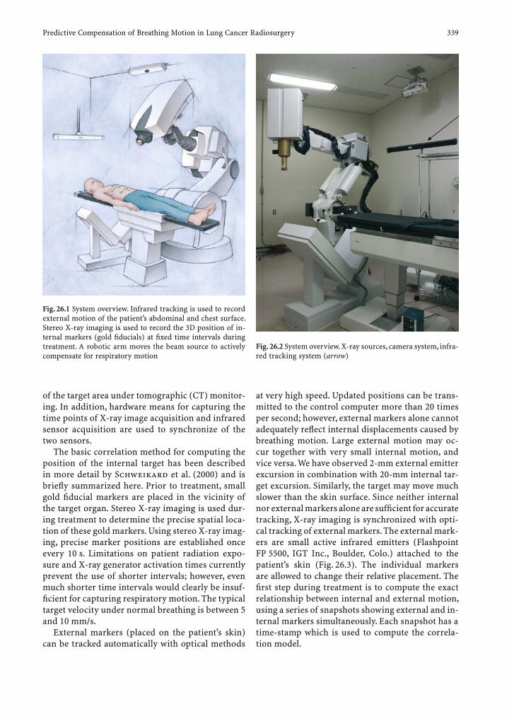
Predictive Compensation of Breathing Motion in Lung Cancer Radiosurgery 339

of the target area under tomographic (CT) monitor-ing. In addition, hardware means for capturing the time points of X-ray image acquisition and infrared sensor acquisition are used to synchronize of the two sensors.

The basic correlation method for computing the position of the internal target has been described in more detail by Schweikard et al. (2000) and is briefl y summarized here. Prior to treatment, small gold fi ducial markers are placed in the vicinity of the target organ. Stereo X-ray imaging is used dur-ing treatment to determine the precise spatial loca-tion of these gold markers. Using stereo X-ray imag-ing, precise marker positions are established once every 10 s. Limitations on patient radiation expo-sure and X-ray generator activation times currently prevent the use of shorter intervals; however, even much shorter time intervals would clearly be insuf-fi cient for capturing respiratory motion. The typical target velocity under normal breathing is between 5 and 10 mm/s.

External markers (placed on the patient’s skin) can be tracked automatically with optical methods

at very high speed. Updated positions can be trans-mitted to the control computer more than 20 times per second; however, external markers alone cannot adequately refl ect internal displacements caused by breathing motion. Large external motion may oc-cur together with very small internal motion, and vice versa. We have observed 2-mm external emitter excursion in combination with 20-mm internal tar-get excursion. Similarly, the target may move much slower than the skin surface. Since neither internal nor external markers alone are suffi cient for accurate tracking, X-ray imaging is synchronized with opti-cal tracking of external markers. The external mark-ers are small active infrared emitters (Flashpoint FP 5500, IGT Inc., Boulder, Colo.) attached to the patient’s skin (Fig. 26.3). The individual markers are allowed to change their relative placement. The fi rst step during treatment is to compute the exact relationship between internal and external motion, using a series of snapshots showing external and in-ternal markers simultaneously. Each snapshot has a time-stamp which is used to compute the correla-tion model.

Fig. 26.1 System overview. Infrared tracking is used to record external motion of the patient’s abdominal and chest surface. Stereo X-ray imaging is used to record the 3D position of in-ternal markers (gold fi ducials) at fi xed time intervals during treatment. A robotic arm moves the beam source to actively compensate for respiratory motion

Fig. 26.2 System overview. X-ray sources, camera system, infra-red tracking system (arrow)

340 A. Schweikard and J. R. Adler

Previous work has addressed the suitability of this combined X-ray/infrared sensor technique as well as the suitability of the robotic gantry for active track-ing. Specifi cally, the imaging methods used for fi du-cial detection, stability and robustness of infrared tracking under radiation exposure, accuracy of the correlation method for different subjects, tracking speed, and inherent time lag have been investigated. A systematic lag of 0.1–0.3 s was established for various motion velocities ranging from 3 to 8 mm per second. At a typical speed of 5 mm, this time lag results in a tracking error of 0.5–1.5 mm. This error purely stems from the inherent system lag.

26.4 Clinical Trials

Twelve patients have been treated with this new sen-sor method. A fully integrated version of the system, including the above prediction scheme has been used in the trials. Figures 26.4–26.6 show the results for representative cases. The fi gure shows the total error in the correlation model; thus, based on the correla-

Fig. 26.3 Infrared emitters, attached to the patient’s chest, are used as external markers. The position of the emitters is tracked by an infrared tracking system (camera attached to the ceiling of the treatment room)

Targ

et Ex

cursi

on an

d Cor

relat

ion

Erro

r (m

m)

node

Correlation Error

Target Excursion

Fig. 26.4 Correlation error and total target excursion. Top curve: motion of the target. Bottom curve: distance between expected position of the gold markers and actual position. The fi rst four images were used for computing the deformation model; hence, the deviation between model and actual posi-tion is zero in the fi rst four nodes

Fig. 26.5 Treatment of a hepatocellular carcinoma with fi ducial-based respiration compensation as described above (left image: before treatment; right image: 3 months after treatment. Total treatment time was 40 min per fraction for three fractions with 80 beam directions and 39 Gy

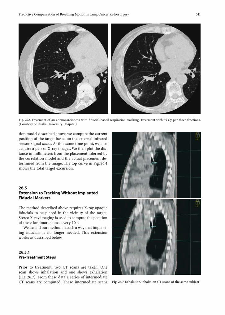
Predictive Compensation of Breathing Motion in Lung Cancer Radiosurgery 341

tion model described above, we compute the current position of the target based on the external infrared sensor signal alone. At this same time point, we also acquire a pair of X-ray images. We then plot the dis-tance in millimeters from the placement inferred by the correlation model and the actual placement de-termined from the image. The top curve in Fig. 26.4 shows the total target excursion.

26.5 Extension to Tracking Without Implanted Fiducial Markers

The method described above requires X-ray opaque fi ducials to be placed in the vicinity of the target. Stereo X-ray imaging is used to compute the position of these landmarks once every 10 s.

We extend our method in such a way that implant-ing fi ducials is no longer needed. This extension works as described below.

26.5.1 Pre-Treatment Steps

Prior to treatment, two CT scans are taken. One scan shows inhalation and one shows exhalation (Fig. 26.7). From these data a series of intermediate CT scans are computed. These intermediate scans

Fig. 26.6 Treatment of an adenocarcinoma with fi ducial-based respiration tracking. Treatment with 39 Gy per three fractions. (Courtesy of Osaka University Hospital)

Fig. 26.7 Exhalation/inhalation CT scans of the same subject

342 A. Schweikard and J. R. Adler

are obtained by interpolating between the inhale and exhale CT scans. This yields a series of 3D scans, showing the respiration process as a 3D motion pic-ture. For each point in this time series, we compute a set of digitally reconstructed radiographs (DRR; e.g., see Murphy 1997; Russakoff 2003). A single DRR is computed by projecting a CT scan from a preselected angle using the known geometry of the X-ray imaging system; thus, a DRR can be regarded as a synthetic X-ray image, obtained by projecting through an existing CT volume. Assume we have 12 time steps in our CT 3D motion picture. For each of the 12 time steps, we compute a number of DRRs for a preselected angle.

26.5.2 Intra-Treatment Steps

During treatment, stereo X-ray images are taken with the stereo X-ray cameras. These images are called live images. When a new live shot is taken, it is com-pared with each of the previously computed DRRs. This comparison selects the best matching DRR in the series. Assume that this best-matching DRR has index number n. Each DRR was computed from one CT scan. Then we can identify the CT scan from which this specifi c DRR (index number n) was gen-erated. This allows for identifying a time step in the 3D CT series, i.e., a respiration state within the re-spiratory cycle. Furthermore, the given DRR (index number n) represents a specifi c angle, under which the present CT scan is seen. This allows for deter-mining the angle under which the patient was seen in the given live shot. Furthermore, computerized comparisons between the live shot and DRRs permit translational shifts to be determined. Overall, if the target is marked in each CT scan, we can identify the exact target location (position, orientation, respira-tion state) at the time the live shot was taken.

This gives only intermittent information on the target location. At the time the comparison of all DRRs with the current live shot is completed, the tar-get may already have moved.

However, our method is nonetheless capable of de-termining the real-time target position with very high accuracy. As in the above fi ducial-based correlation method, a real-time sensor is used to report informa-tion on the current state of respiration in real time. This information is correlated to the target location computed by the comparison between the live shot and DRRs. To this end, the live shot has a time stamp, and we can determine which reading of the real-time

sensor corresponded to this point in time. Repeating this time stamp synchronization, we can obtain a com-plete correlation model, correlating target motion to the readings of the real-time sensor, without internal fi ducials. We do not need real-time elastic registration but can still account for organ deformation.

26.6 Discussion and Conclusion

The described technique combines information from two sensors: X-ray imaging and infrared tracking. Both sensors have very characteristic advantages in our application. Stereo X-ray imaging can determine the exact location of fi ducial markers via automatic image analysis. Our tracking method (X-ray imaging with time stamps, combined with infrared sensing) does not require that the location of the infrared emitters be computed in the X-ray images. The in-frared emitters do not even have to be visible in the X-ray images. This avoids occlusions and simplifi es image processing considerably. The observed motion of external infrared markers (4–20 mm) is large when compared with the noise range of infrared position computation (<0.01 mm); thus, the ratio between noise and signal is adequate for following the respi-ratory cycle. Our method currently requires fi ducial markers be implanted prior to treatment. While this procedure is more invasive than direct (non-stereo-taxic) radiation therapy, the gain in localization ac-curacy should justify this added invasiveness. It is possible that advanced image processing methods can ultimately obviate the need for implanted fi du-cial markers.

The described method obtains an overall correla-tion error of below 2 mm throughout the entire treat-ment of 70 min, whereas the total target motion was over 10 mm. This suggests that our method is capa-ble of reducing safety margins by a very substantial amount.

The experiments confi rm our hypothesis that respiratory motion of internal organs can be cor-related to visible external motion, provided that the correlation model can be updated automatically in real-time by intra-operative images. This suggests that any dose margin placed around a tumor to compensate for respiratory motion can be reduced by a very substantial amount. Since dose is directly proportional to volume, this could allow for higher doses in the tumor, and much lower dose in sur-rounding healthy tissue. For a variety of cancers

Predictive Compensation of Breathing Motion in Lung Cancer Radiosurgery 343

with grim prognosis, this robotic technique could thus lead to far-reaching improvements in clinical outcome.

References

Adler JR, Schweikard A, Tombropoulos R, Latombe J-C (1999) Image-guided robotic radiosurgery. In: Kondziolka D (ed) Radiosurgery. Karger, New York

Haykin S (1996) Adaptive fi lter theory. Prentice-Hall LondonKubo HD, Hill BC (1996) Respiration gated radiotherapy treat-

ment: a technical study. Phys Med Biol 41:93–101Lujan AE, Larsen EW, Balter JM, Haken RKT (1999) A method

for incorporating organ motion due to breathing into 3D dose calculations. Med Phys 26:715–720

Morrill SM, Langer M, Lane RG (1996) Real-time couch com-pensation for intra-treatment organ motion: theoretical advantages. Med Phys 23:1083

Murphy M (1997) An automatic six-degree-of-freedom image registration algorithm for image-guided frameless stereo-taxic radiosurgery. Med Phys 24:857–866

Riesner S (2004) Korrelations- und Prädiktionsverfahren zur

Lageverfolgung in der perkutanen Rodioonkologie, Disser-tation, Informatik, TU München

Russakoff DB, Rohlfi ng T et al. (2003) Fast calculation of digi-tally reconstructed radiographs using light fi elds. Medical Imaging 2003. In: Proc SPIE, vol 5032

Schweikard A, Bodduluri M, Adler JR (1998) Planning for camera-guided robotic radiosurgery. IEEE Trans Robot Autom 14:951–962

Schweikard A, Glosser G, Bodduluri M, Murphy M, Adler JR (2000) Robotic motion compensation for respiratory movement during radiosurgery. Special issue on planning and image guidance in radiation therapy. Comput Aided Surg 5(4):263–277

Sontag MR, Lai ZW et al. (1996) Characterization of respiratory motion for pedriatic conformal 3D therapy. Med Phys 23:1082

Tada T, Minakuchi K et al. (1998) Lung cancer: intermittent irradiation synchronized with respiratory motion: results of a pilot study. Radiology 207:779–783

Webb S (1993) The physics of three-dimensional radiation therapy. Institute of Physics Publishing, Bristol

Webb S (2000) Conformal intensity-modulated radiotherapy (IMRT) delivered by robotic linac-conformality versus effi -ciency of dose delivery. Phys Med Biol 45:1715–1730

Winston KR, Lutz W (1988) Linear accelerator as a neuro-surgical tool for stereotactic radiosurgery. Neurosurgery 22:454–464

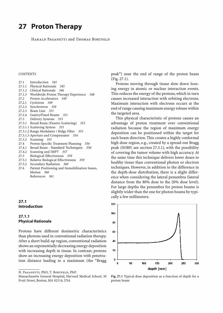
27.1 Introduction

27.1.1 Physical Rationale

Protons have different dosimetric characteristics than photons used in conventional radiation therapy. After a short build-up region, conventional radiation shows an exponentially decreasing energy deposition with increasing depth in tissue. In contrast, protons show an increasing energy deposition with penetra-tion distance leading to a maximum (the “Bragg

peak”) near the end of range of the proton beam (Fig. 27.1).

Protons moving through tissue slow down loos-ing energy in atomic or nuclear interaction events. This reduces the energy of the protons, which in turn causes increased interaction with orbiting electrons. Maximum interaction with electrons occurs at the end of range causing maximum energy release within the targeted area.

This physical characteristic of protons causes an advantage of proton treatment over conventional radiation because the region of maximum energy deposition can be positioned within the target for each beam direction. This creates a highly conformal high dose region, e.g., created by a spread-out Bragg peak (SOBP; see section 27.3.1), with the possibility of covering the tumor volume with high accuracy. At the same time this technique delivers lower doses to healthy tissue than conventional photon or electron techniques. However, in addition to the difference in the depth-dose distribution, there is a slight differ-ence when considering the lateral penumbra (lateral distance from the 80% dose to the 20% dose level). For large depths the penumbra for proton beams is slightly wider than the one for photon beams by typi-cally a few millimeters.

CONTENTS

27.1 Introduction 34527.1.1 Physical Rationale 34527.1.2 Clinical Rationale 34627.1.3 Worldwide Proton Therapy Experience 34827.2 Proton Accelerators 34927.2.1 Cyclotron 34927.2.2 Synchrotron 35027.2.3 Beam Line 35127.2.4 Gantry/Fixed Beams 35127.3 Delivery Systems 35327.3.1 Broad Beam (Passive Scattering) 35327.3.1.1 Scattering System 35327.3.1.2 Range Modulator / Ridge Filter 35327.3.1.3 Aperture and Compensator 35427.3.2 Scanning 35527.4 Proton-Specifi c Treatment Planning 35627.4.1 Broad Beam - Standard Techniques 35627.4.2 Scanning and IMPT 35727.5 Biological Effectiveness 35927.5.1 Relative Biological Effectiveness 35927.5.2 Secondary Radiation 36027.6 Patient Positioning and Immobilization Issues, Motion 360 References 361

Fig. 27.1 Typical dose deposition as a function of depth for a proton beam

Proton Therapy 345

27 Proton Therapy

Harald Paganetti and Thomas Bortfeld

H. Paganetti, PhD, T. Bortfeld, PhDMassachusetts General Hospital, Harvard Medical School, 30 Fruit Street, Boston, MA 02114, USA

27.1.2 Clinical Rationale

The rationale for the clinical use of proton beams is the feasibility of delivering higher doses to the tumor, leading to an increased tumor control probability (TCP; Niemierko et al. 1992). This is possible due to the irradiation of a smaller volume of normal tissues compared with other modalities. Due to the reduced treatment volume and a lower integral dose, patient tolerance is increased. Like other highly conformal therapy techniques, proton therapy is of particular interest for those tumors located close to serially organized tissues where a small local overdose can cause fatal complication such as most tumors close to the spinal cord. Irregular-shaped lesions near critical structures are well suited for protons.

Proton therapy has been applied for the treatment of various disease sites (Delaney et al. 2003) includ-ing paranasal sinus tumors (Thornton et al. 1998), chordoma (Benk et al. 1995; Terahara et al. 1999), chondrosarcoma (Rosenberg et al. 1999), menin-gioma (Hug et al. 2000; Wenkel et al. 2000), prostate (Hara et al. 2004; Slater et al. 2004a, b), and lung tu-mors (Shioyama et al. 2003). Clinical gains with pro-tons have long been realized in the treatment of uveal melanomas, sarcomas of the base of skull (Weber et al. 2004), and sarcomas of the paravertebral region. Proton radiosurgery has been used to treat large arte-rial venous malformations as well as other intracra-nial lesions (Harsh et al. 1999).

Treatment plan comparisons show that protons offer potential gains for many sites. Comparisons of treatment modalities (protons vs photons) have been made on the basis of TCP and normal tissue compli-cation probability (NCTP) calculations for cranial ir-radiation of childhood optic nerve gliomas by Fuss et al. (2000). Also, advantages of proton plans compared with photon plans have been shown for pediatric optic pathway gliomas (Fuss et al. 1999) and for pediatric medulloblastoma/primitive neuro-ectodermal tumors (Miralbell et al. 1997). Here, proton therapy offered a high degree of conformity to the target volumes and steep dose gradients, thus leading to substantial nor-mal tissue sparing in high- and low-dose areas. Studies on various central nervous system tumors and pediat-ric patients with low-grade astrocytoma revealed that acute or early/late side effects were low (McAllister et al. 1997; Hug and Slater 1999). Another target used for comparative treatment planning is glioblastoma multiforme (Tatsuzaki et al. 1992a) where, due to a highly radioresistant tumor mass and due to extensive microscopic invasion, high doses to critical structures

are diffi cult to avoid. A comparison of proton and X-ray treatment planning for prostate cancer has been pub-lished by LEE et al. (1994). Other authors studied X-ray and proton irradiation of esophageal cancer (Isacsson et al. 1998), locally advanced rectal cancer (Isacsson et al. 1996), and paraspinal tumors (Isacsson et al. 1997) showing that protons have therapeutic advan-tages over conventional therapy based on TCP and NTCP calculations. Osteo- and chondrogenic tumors of the axial skeleton, rare tumors at high risk for local failure, were studied for combined proton and photon radiation therapy (Hug et al. 1995). The potential ad-vantages of protons has also been discussed for vari-ous other types of tumors (Archambeau et al. 1992; Levin 1992; Miralbell et al. 1992; Nowakowski et al. 1992; Slater et al. 1992a, b; Smit 1992; Tatsuzaki et al. 1992a, b; Wambersie et al. 1992; Lee et al. 1994; Lin et al. 2000).

For advanced head and neck tumors a treatment plan comparison was done by Cozzi et al. (2001) for fi ve patients using 3D conformal and intensity modulated photon therapy and proton therapy. They distinguished between passive and active modulated proton beams (see section 27.4). They concluded that looking at target coverage and tumor control proba-bility there are only small differences between highly sophisticated techniques like protons or intensity modulated photons if the comparison is made against good conformal treatment modalities with conven-tional photon beams. The situation was judged to be quite different if organs at risk were considered.

A treatment plan comparison for conventional proton, scanned proton, and intensity-modulated photon radiotherapy was performed by Lomax et al. (1999) using CT scans and planning information for nine patients with varying indications and le-sion sites. The results were analyzed using a variety of dose- and volume-based parameters. They found that the use of protons could lead to a reduction of the integral dose by a factor of three compared with standard photon techniques and a factor of two compared with intensity-modulated photon plans. Furthermore, optimized treatment plans for inten-sity-modulated X-ray therapy (IMXT), very high energy electron therapy, and intensity-modulated proton therapy (IMPT) were compared for prostate cancer (Yeboah and Sandison 2002). It was con-cluded that IMPT delivered a mean rectal dose and a bladder dose that was much lower than achievable with the other two modalities. The IMPT was also su-perior in target coverage. Figure 27.2 demonstrates the conformality achievable with conventional pro-ton therapy for various body sites.

H. Paganetti and T. Bortfeld346

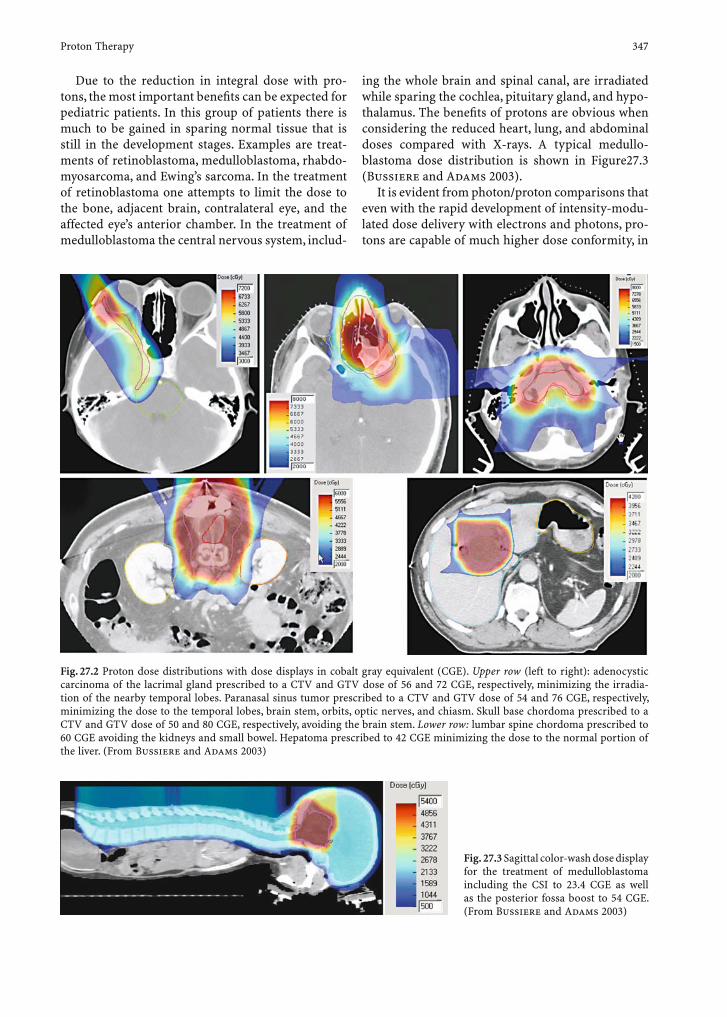
Due to the reduction in integral dose with pro-tons, the most important benefi ts can be expected for pediatric patients. In this group of patients there is much to be gained in sparing normal tissue that is still in the development stages. Examples are treat-ments of retinoblastoma, medulloblastoma, rhabdo-myosarcoma, and Ewing’s sarcoma. In the treatment of retinoblastoma one attempts to limit the dose to the bone, adjacent brain, contralateral eye, and the affected eye’s anterior chamber. In the treatment of medulloblastoma the central nervous system, includ-

ing the whole brain and spinal canal, are irradiated while sparing the cochlea, pituitary gland, and hypo-thalamus. The benefi ts of protons are obvious when considering the reduced heart, lung, and abdominal doses compared with X-rays. A typical medullo-blastoma dose distribution is shown in Figure27.3 (Bussiere and Adams 2003).

It is evident from photon/proton comparisons that even with the rapid development of intensity-modu-lated dose delivery with electrons and photons, pro-tons are capable of much higher dose conformity, in

Fig. 27.3 Sagittal color-wash dose display for the treatment of medulloblastoma including the CSI to 23.4 CGE as well as the posterior fossa boost to 54 CGE. (From Bussiere and Adams 2003)

Fig. 27.2 Proton dose distributions with dose displays in cobalt gray equivalent (CGE). Upper row (left to right): adenocystic carcinoma of the lacrimal gland prescribed to a CTV and GTV dose of 56 and 72 CGE, respectively, minimizing the irradia-tion of the nearby temporal lobes. Paranasal sinus tumor prescribed to a CTV and GTV dose of 54 and 76 CGE, respectively, minimizing the dose to the temporal lobes, brain stem, orbits, optic nerves, and chiasm. Skull base chordoma prescribed to a CTV and GTV dose of 50 and 80 CGE, respectively, avoiding the brain stem. Lower row: lumbar spine chordoma prescribed to 60 CGE avoiding the kidneys and small bowel. Hepatoma prescribed to 42 CGE minimizing the dose to the normal portion of the liver. (From Bussiere and Adams 2003)

Proton Therapy 347

particular for intensity-modulated proton techniques (Lomax et al. 1999; Lomax et al. 2003a, b; Weber et al. 2004). The reduction of integral dose with protons is also signifi cant. Although it is true that the clinical relevance of low doses to large volumes is not well known (except perhaps in organs with a parallel or near parallel architecture), there are cases where a re-duction in overall normal tissue dose is proven to be relevant, e.g., for pediatric patients (Lin et al. 2000).

27.1.3 Worldwide Proton Therapy Experience

Robert Wilson fi rst proposed the use of protons for radiation therapy at Harvard in 1946 (Wilson 1946).

The fi rst patient was treated in 1954 at Lawrence Berkeley Laboratory (Tobias et al. 1958). About 40,000 patients have received proton therapy to date worldwide (see Table 27.1; Sisterson 2004).

Although the number of patients being treated with protons is steadily increasing, as are the num-ber of facilities operating worldwide, it is still only a small fraction of radiotherapy patients overall that are treated with protons. One reason for this is the cost of a proton facility. Sophisticated proton therapy is presently, and is likely to continue to be, more ex-pensive than sophisticated (i.e., intensity-modulated) X-ray therapy. The construction cost of a current two-gantry proton facility, complete with the equip-ment, was estimated to be about four times the cost of a two-linac X-ray facility (Goitein and Jermann

Table 27.1 Worldwide proton therapy experience as of July 2004. (From SISTERSON 2004)

Institution Location First treatment Last treatment No. of patients Date of total

Berkeley California, USA 1954 1957 30

Uppsala Sweden 1957 1976 73

Harvard Massachusetts, USA 1961 2002 9116

Dubna Russia 1967 1996 124

ITEP, Moscow Russia 1969 3748 June 2004

St. Petersburg Russia 1975 1145 April 2004

Chiba Japan 1979 145 April 2002

PMRC(1), Tsukuba Japan 1983 2000 700

PSI (72 MeV) Switzerland 1984 4066 June 2004

Dubna Russia 1999 191 Nov. 2003

Uppsala Sweden 1989 418 Jan. 2004

Clatterbridge UK 1989 1287 Dec. 2003

Loma Linda California, USA 1990 9282 July 2004

Louvain-la-Neuve Belgium 1991 1993 21

Nice France 1991 2555 April 2004

Orsay France 1991 2805 Dec. 2003

iThemba LABS South Africa 1993 446 Dec. 2003

MPRI(1) Indiana, USA 1993 1999 34

UCSF – CNL California, USA 1994 632 June 2004

TRIUMF Canada 1995 89 Dec. 2003

PSI (200 MeV) Switzerland 1996 166 Dec. 2003

H.M.I, Berlin Germany 1998 437 Dec. 2003

NCC, Kashiwa Japan 1998 270 June 2004

HIBMC, Hyogo Japan 2001 359 June 2004

PMRC(2), Tsukuba Japan 2001 492 July 2004

NPTC, MGH Massachusetts, USA 2001 800 July 2004

INFN-LNS, Catania Italy 2002 77 June 2004

WERC Japan 2002 14 Dec. 2003

Shizuoka Japan 2003 69 July 2004

MPRI(2) Indiana, USA 2004 21 July 2004

Total 39,612

H. Paganetti and T. Bortfeld348

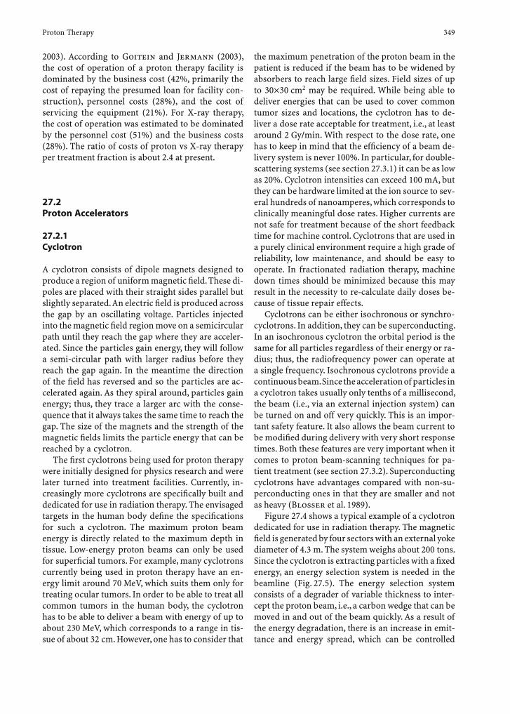
2003). According to Goitein and Jermann (2003), the cost of operation of a proton therapy facility is dominated by the business cost (42%, primarily the cost of repaying the presumed loan for facility con-struction), personnel costs (28%), and the cost of servicing the equipment (21%). For X-ray therapy, the cost of operation was estimated to be dominated by the personnel cost (51%) and the business costs (28%). The ratio of costs of proton vs X-ray therapy per treatment fraction is about 2.4 at present.

27.2 Proton Accelerators

27.2.1 Cyclotron

A cyclotron consists of dipole magnets designed to produce a region of uniform magnetic fi eld. These di-poles are placed with their straight sides parallel but slightly separated. An electric fi eld is produced across the gap by an oscillating voltage. Particles injected into the magnetic fi eld region move on a semicircular path until they reach the gap where they are acceler-ated. Since the particles gain energy, they will follow a semi-circular path with larger radius before they reach the gap again. In the meantime the direction of the fi eld has reversed and so the particles are ac-celerated again. As they spiral around, particles gain energy; thus, they trace a larger arc with the conse-quence that it always takes the same time to reach the gap. The size of the magnets and the strength of the magnetic fi elds limits the particle energy that can be reached by a cyclotron.

The fi rst cyclotrons being used for proton therapy were initially designed for physics research and were later turned into treatment facilities. Currently, in-creasingly more cyclotrons are specifi cally built and dedicated for use in radiation therapy. The envisaged targets in the human body defi ne the specifi cations for such a cyclotron. The maximum proton beam energy is directly related to the maximum depth in tissue. Low-energy proton beams can only be used for superfi cial tumors. For example, many cyclotrons currently being used in proton therapy have an en-ergy limit around 70 MeV, which suits them only for treating ocular tumors. In order to be able to treat all common tumors in the human body, the cyclotron has to be able to deliver a beam with energy of up to about 230 MeV, which corresponds to a range in tis-sue of about 32 cm. However, one has to consider that

the maximum penetration of the proton beam in the patient is reduced if the beam has to be widened by absorbers to reach large fi eld sizes. Field sizes of up to 30×30 cm2 may be required. While being able to deliver energies that can be used to cover common tumor sizes and locations, the cyclotron has to de-liver a dose rate acceptable for treatment, i.e., at least around 2 Gy/min. With respect to the dose rate, one has to keep in mind that the effi ciency of a beam de-livery system is never 100%. In particular, for double-scattering systems (see section 27.3.1) it can be as low as 20%. Cyclotron intensities can exceed 100 mA, but they can be hardware limited at the ion source to sev-eral hundreds of nanoamperes, which corresponds to clinically meaningful dose rates. Higher currents are not safe for treatment because of the short feedback time for machine control. Cyclotrons that are used in a purely clinical environment require a high grade of reliability, low maintenance, and should be easy to operate. In fractionated radiation therapy, machine down times should be minimized because this may result in the necessity to re-calculate daily doses be-cause of tissue repair effects.

Cyclotrons can be either isochronous or synchro-cyclotrons. In addition, they can be superconducting. In an isochronous cyclotron the orbital period is the same for all particles regardless of their energy or ra-dius; thus, the radiofrequency power can operate at a single frequency. Isochronous cyclotrons provide a continuous beam. Since the acceleration of particles in a cyclotron takes usually only tenths of a millisecond, the beam (i.e., via an external injection system) can be turned on and off very quickly. This is an impor-tant safety feature. It also allows the beam current to be modifi ed during delivery with very short response times. Both these features are very important when it comes to proton beam-scanning techniques for pa-tient treatment (see section 27.3.2). Superconducting cyclotrons have advantages compared with non-su-perconducting ones in that they are smaller and not as heavy (Blosser et al. 1989).

Figure 27.4 shows a typical example of a cyclotron dedicated for use in radiation therapy. The magnetic fi eld is generated by four sectors with an external yoke diameter of 4.3 m. The system weighs about 200 tons. Since the cyclotron is extracting particles with a fi xed energy, an energy selection system is needed in the beamline (Fig. 27.5). The energy selection system consists of a degrader of variable thickness to inter-cept the proton beam, i.e., a carbon wedge that can be moved in and out of the beam quickly. As a result of the energy degradation, there is an increase in emit-tance and energy spread, which can be controlled

Proton Therapy 349

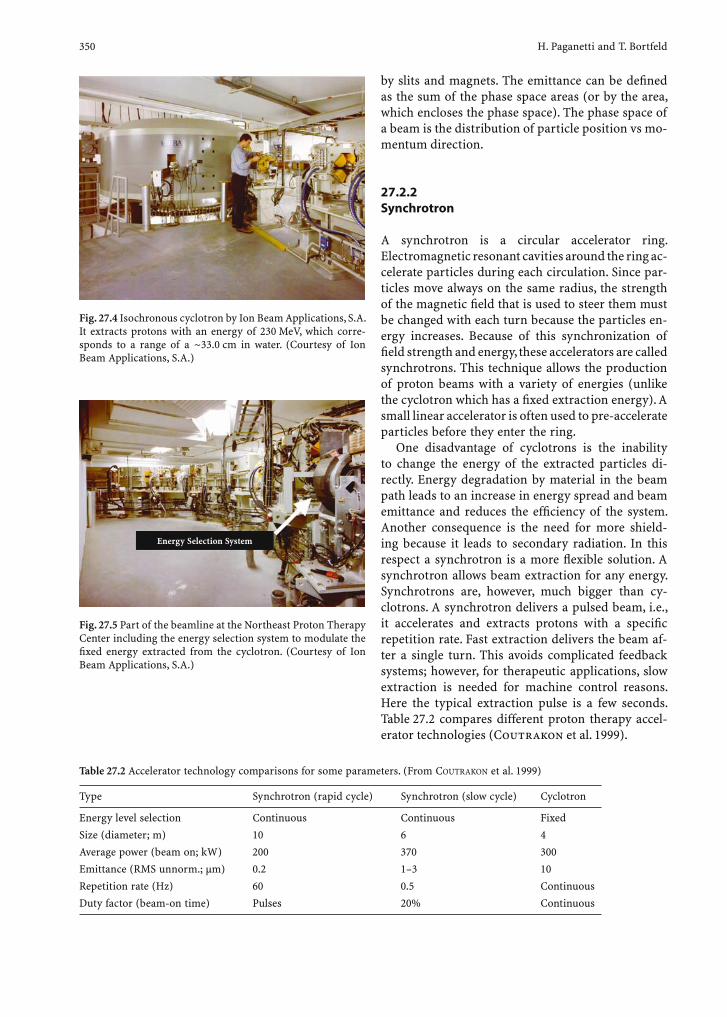
by slits and magnets. The emittance can be defi ned as the sum of the phase space areas (or by the area, which encloses the phase space). The phase space of a beam is the distribution of particle position vs mo-mentum direction.

27.2.2 Synchrotron

A synchrotron is a circular accelerator ring. Electromagnetic resonant cavities around the ring ac-celerate particles during each circulation. Since par-ticles move always on the same radius, the strength of the magnetic fi eld that is used to steer them must be changed with each turn because the particles en-ergy increases. Because of this synchronization of fi eld strength and energy, these accelerators are called synchrotrons. This technique allows the production of proton beams with a variety of energies (unlike the cyclotron which has a fi xed extraction energy). A small linear accelerator is often used to pre-accelerate particles before they enter the ring.

One disadvantage of cyclotrons is the inability to change the energy of the extracted particles di-rectly. Energy degradation by material in the beam path leads to an increase in energy spread and beam emittance and reduces the effi ciency of the system. Another consequence is the need for more shield-ing because it leads to secondary radiation. In this respect a synchrotron is a more fl exible solution. A synchrotron allows beam extraction for any energy. Synchrotrons are, however, much bigger than cy-clotrons. A synchrotron delivers a pulsed beam, i.e., it accelerates and extracts protons with a specifi c repetition rate. Fast extraction delivers the beam af-ter a single turn. This avoids complicated feedback systems; however, for therapeutic applications, slow extraction is needed for machine control reasons. Here the typical extraction pulse is a few seconds. Table 27.2 compares different proton therapy accel-erator technologies (Coutrakon et al. 1999).

Table 27.2 Accelerator technology comparisons for some parameters. (From COUTRAKON et al. 1999)

Type Synchrotron (rapid cycle) Synchrotron (slow cycle) Cyclotron

Energy level selection Continuous Continuous Fixed

Size (diameter; m) 10 6 4

Average power (beam on; kW) 200 370 300

Emittance (RMS unnorm.; µm) 0.2 1–3 10

Repetition rate (Hz) 60 0.5 Continuous

Duty factor (beam-on time) Pulses 20% Continuous

Energy Selection System

Fig. 27.5 Part of the beamline at the Northeast Proton Therapy Center including the energy selection system to modulate the fi xed energy extracted from the cyclotron. (Courtesy of Ion Beam Applications, S.A.)

Fig. 27.4 Isochronous cyclotron by Ion Beam Applications, S.A. It extracts protons with an energy of 230 MeV, which corre-sponds to a range of a ~33.0 cm in water. (Courtesy of Ion Beam Applications, S.A.)

H. Paganetti and T. Bortfeld350

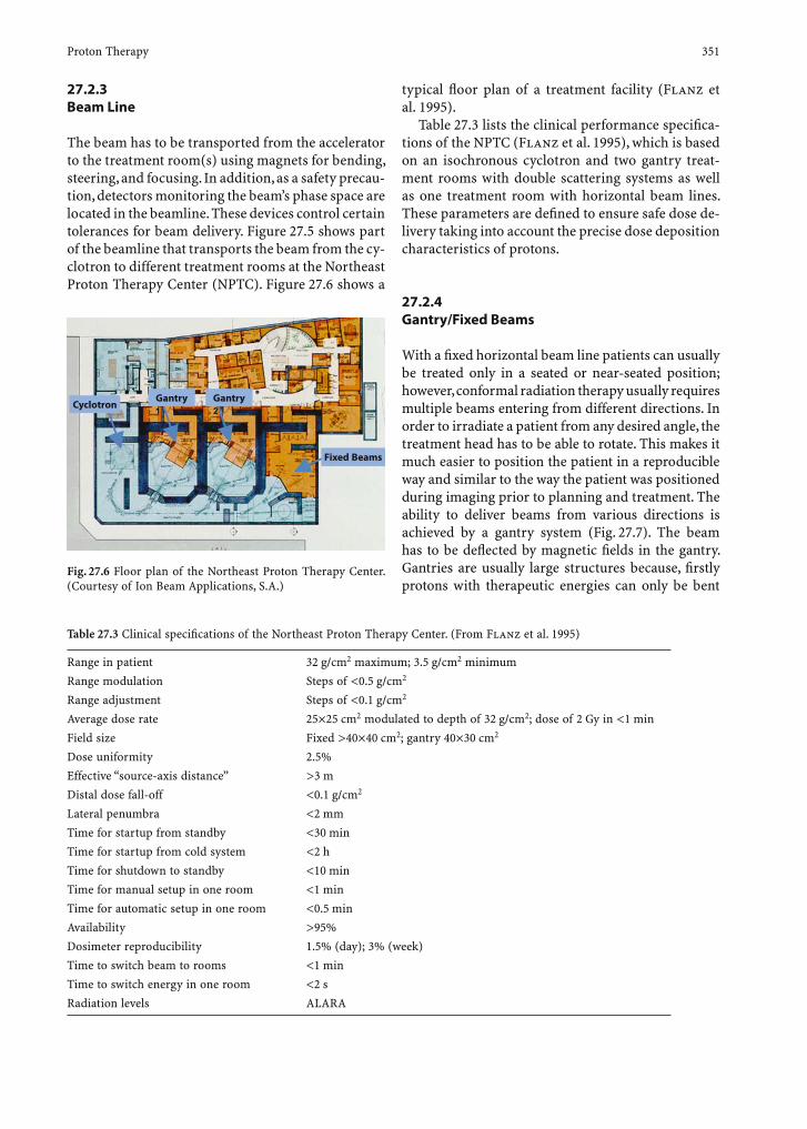
27.2.3 Beam Line

The beam has to be transported from the accelerator to the treatment room(s) using magnets for bending, steering, and focusing. In addition, as a safety precau-tion, detectors monitoring the beam’s phase space are located in the beamline. These devices control certain tolerances for beam delivery. Figure 27.5 shows part of the beamline that transports the beam from the cy-clotron to different treatment rooms at the Northeast Proton Therapy Center (NPTC). Figure 27.6 shows a

typical fl oor plan of a treatment facility (Flanz et al. 1995).

Table 27.3 lists the clinical performance specifi ca-tions of the NPTC (Flanz et al. 1995), which is based on an isochronous cyclotron and two gantry treat-ment rooms with double scattering systems as well as one treatment room with horizontal beam lines. These parameters are defi ned to ensure safe dose de-livery taking into account the precise dose deposition characteristics of protons.

27.2.4 Gantry/Fixed Beams

With a fi xed horizontal beam line patients can usually be treated only in a seated or near-seated position; however, conformal radiation therapy usually requires multiple beams entering from different directions. In order to irradiate a patient from any desired angle, the treatment head has to be able to rotate. This makes it much easier to position the patient in a reproducible way and similar to the way the patient was positioned during imaging prior to planning and treatment. The ability to deliver beams from various directions is achieved by a gantry system (Fig. 27.7). The beam has to be defl ected by magnetic fi elds in the gantry. Gantries are usually large structures because, fi rstly protons with therapeutic energies can only be bent

Fig. 27.6 Floor plan of the Northeast Proton Therapy Center. (Courtesy of Ion Beam Applications, S.A.)

Fixed Beams

GantryGantryCyclotron

Table 27.3 Clinical specifi cations of the Northeast Proton Therapy Center. (From Flanz et al. 1995)

Range in patient 32 g/cm2 maximum; 3.5 g/cm2 minimum

Range modulation Steps of <0.5 g/cm2

Range adjustment Steps of <0.1 g/cm2

Average dose rate 25×25 cm2 modulated to depth of 32 g/cm2; dose of 2 Gy in <1 min

Field size Fixed >40×40 cm2; gantry 40×30 cm2

Dose uniformity 2.5%

Effective “source-axis distance” >3 m

Distal dose fall-off <0.1 g/cm2

Lateral penumbra <2 mm

Time for startup from standby <30 min

Time for startup from cold system <2 h

Time for shutdown to standby <10 min

Time for manual setup in one room <1 min

Time for automatic setup in one room <0.5 min

Availability >95%

Dosimeter reproducibility 1.5% (day); 3% (week)

Time to switch beam to rooms <1 min

Time to switch energy in one room <2 s

Radiation levels ALARA

Proton Therapy 351

with large radii, and secondly, beam-monitoring and beam-shaping devices have to be positioned inside the treatment head affecting the size of the nozzle. The nozzle at the NPTC has a length of about 2.5 m, which results in a distance between isocenter and beam en-tering the gantry of about 3 m. Eccentric gantries are used to reduce the size (Pedroni et al. 1995). To en-sure precise dose delivery the mechanics of the gantry has to be able to keep the isocenter of rotation always within 1 mm under all rotation angles. This requires careful design of the mechanical structure since the overall weight can be several tens of tons.

Treatment nozzles consist of various components for beam shaping and beam monitoring (Fig. 27.8). Beam monitoring ionization chambers detect de-viations in beam position, measure the total beam

current, and check the beam size and uniformity. Ionization chambers may consist of parallel electrode planes divided into horizontal and vertical strips that allow the quantifi cation of the lateral uniformity of the radiation fi eld. These strips are integrated separately to collect the current in each strip. Such ionization chamber can be used at nozzle entrance, i.e., where the proton beam exits the beam line, to monitors the size of the initial beam spot and the angular distribu-tion of the beam. Beam-shaping devices in the nozzle are scatterers, absorbers, and other patient-specifi c hardware. The nozzle also has a snout that permits mounting and positioning of a fi eld-specifi c aperture and compensator along the beam axis. The snout of the nozzle is telescopic to adjust the air gap between the fi nal collimator or compensator and the patient.

Fig. 27.7 One of the gantries at the Northeast Proton Therapy Center. Left: the gantry structure during construction with the steel assembly being visible. Right: the gantry treatment room during treatment. The beam delivery nozzle is able to rotate 360° around the movable patient couch. (Courtesy of Ion Beam Applications, S.A.).

Fig. 27.8 The nozzle at the NPTC (Paganetti et al. 2004b). Beam moni-toring devices are ionization chambers (IC) and a range verifi er (multi-layer Faraday cup). Beam-shaping devices are scattering systems, range modula-tors, and wobbling magnets. Variable collimators (“jaws”) and the snout de-termine the fi eld size

H. Paganetti and T. Bortfeld352

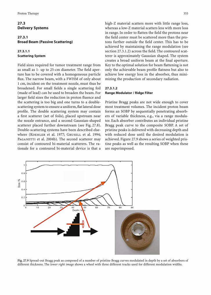
27.3 Delivery Systems

27.3.1 Broad Beam (Passive Scattering)

27.3.1.1 Scattering System

Field sizes required for tumor treatment range from as small as 1- up to 25-cm diameter. The fi eld aper-ture has to be covered with a homogeneous particle fl ux. The narrow beam, with a FWHM of only about 1 cm, incident on the treatment nozzle, must thus be broadened. For small fi elds a single scattering foil (made of lead) can be used to broaden the beam. For larger fi eld sizes the reduction in proton fl uence and the scattering is too big and one turns to a double-scattering system to ensure a uniform, fl at lateral dose profi le. The double scattering system may contain a fi rst scatterer (set of foils), placed upstream near the nozzle entrance, and a second Gaussian-shaped scatterer placed further downstream (see Fig. 27.8). Double-scattering systems have been described else-where (Koehler et al. 1977; Grusell et al. 1994; Paganetti et al. 2004b). The second scatterer may consist of contoured bi-material scatterers. The ra-tionale for a contoured bi-material device is that a

high-Z material scatters more with little range loss, whereas a low-Z material scatters less with more loss in range. In order to fl atten the fi eld the protons near the fi eld center must be scattered more than the pro-tons further outside the fi eld center. This has to be achieved by maintaining the range modulation (see section 27.3.1.2) across the fi eld. The contoured scat-terer is approximately Gaussian shaped. The system creates a broad uniform beam at the fi nal aperture. Key to the optimal solution for beam fl attening is not only the achievable beam profi le fl atness but also to achieve low energy loss in the absorber, thus mini-mizing the production of secondary radiation.

27.3.1.2 Range Modulator / Ridge Filter

Pristine Bragg peaks are not wide enough to cover most treatment volumes. The incident proton beam forms an SOBP by sequentially penetrating absorb-ers of variable thickness, e.g., via a range modula-tor. Each absorber contributes an individual pristine Bragg peak curve to the composite SOBP. A set of pristine peaks is delivered with decreasing depth and with reduced dose until the desired modulation is achieved. Figure 27.9 shows a series of weighted pris-tine peaks as well as the resulting SOBP when these are superimposed.

Fig. 27.9 Spread-out Bragg peak as composed of a number of pristine Bragg curves modulated in depth by a set of absorbers of different thickness. The lower right image shows a wheel with three different tracks used for different modulation widths.

Proton Therapy 353

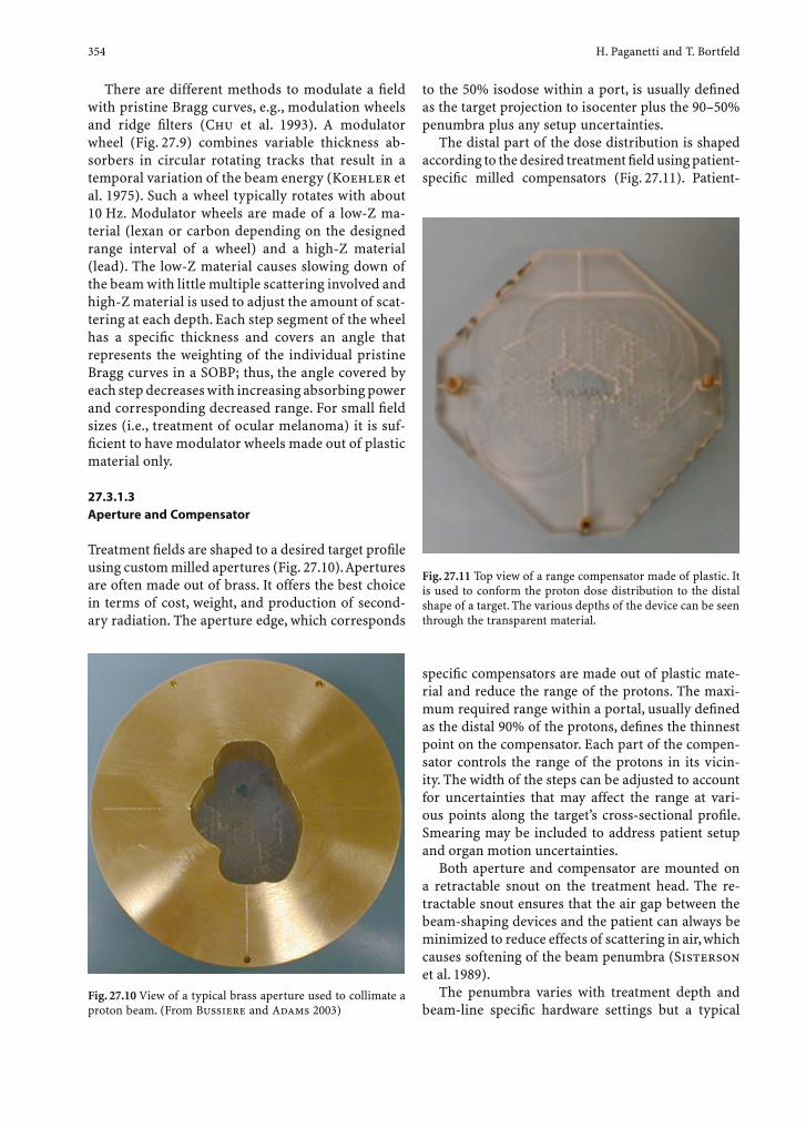
There are different methods to modulate a fi eld with pristine Bragg curves, e.g., modulation wheels and ridge fi lters (Chu et al. 1993). A modulator wheel (Fig. 27.9) combines variable thickness ab-sorbers in circular rotating tracks that result in a temporal variation of the beam energy (Koehler et al. 1975). Such a wheel typically rotates with about 10 Hz. Modulator wheels are made of a low-Z ma-terial (lexan or carbon depending on the designed range interval of a wheel) and a high-Z material (lead). The low-Z material causes slowing down of the beam with little multiple scattering involved and high-Z material is used to adjust the amount of scat-tering at each depth. Each step segment of the wheel has a specifi c thickness and covers an angle that represents the weighting of the individual pristine Bragg curves in a SOBP; thus, the angle covered by each step decreases with increasing absorbing power and corresponding decreased range. For small fi eld sizes (i.e., treatment of ocular melanoma) it is suf-fi cient to have modulator wheels made out of plastic material only.

27.3.1.3 Aperture and Compensator

Treatment fi elds are shaped to a desired target profi le using custom milled apertures (Fig. 27.10). Apertures are often made out of brass. It offers the best choice in terms of cost, weight, and production of second-ary radiation. The aperture edge, which corresponds

to the 50% isodose within a port, is usually defi ned as the target projection to isocenter plus the 90–50% penumbra plus any setup uncertainties.

The distal part of the dose distribution is shaped according to the desired treatment fi eld using patient-specifi c milled compensators (Fig. 27.11). Patient-

Fig. 27.10 View of a typical brass aperture used to collimate a proton beam. (From Bussiere and Adams 2003)

Fig. 27.11 Top view of a range compensator made of plastic. It is used to conform the proton dose distribution to the distal shape of a target. The various depths of the device can be seen through the transparent material.

specifi c compensators are made out of plastic mate-rial and reduce the range of the protons. The maxi-mum required range within a portal, usually defi ned as the distal 90% of the protons, defi nes the thinnest point on the compensator. Each part of the compen-sator controls the range of the protons in its vicin-ity. The width of the steps can be adjusted to account for uncertainties that may affect the range at vari-ous points along the target’s cross-sectional profi le. Smearing may be included to address patient setup and organ motion uncertainties.

Both aperture and compensator are mounted on a retractable snout on the treatment head. The re-tractable snout ensures that the air gap between the beam-shaping devices and the patient can always be minimized to reduce effects of scattering in air, which causes softening of the beam penumbra (Sisterson et al. 1989).

The penumbra varies with treatment depth and beam-line specifi c hardware settings but a typical

H. Paganetti and T. Bortfeld354

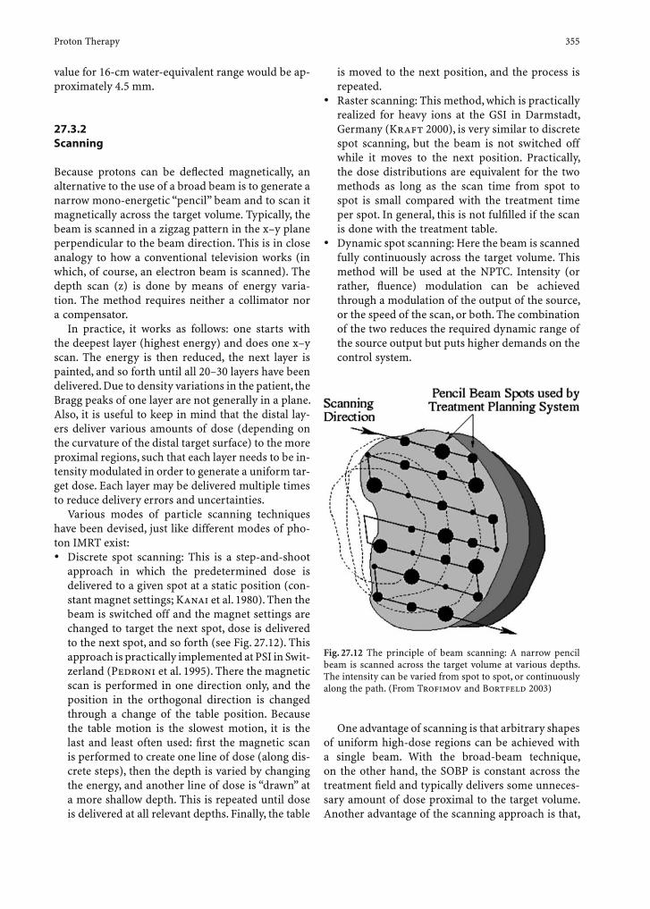
value for 16-cm water-equivalent range would be ap-proximately 4.5 mm.

27.3.2 Scanning

Because protons can be defl ected magnetically, an alternative to the use of a broad beam is to generate a narrow mono-energetic “pencil” beam and to scan it magnetically across the target volume. Typically, the beam is scanned in a zigzag pattern in the x–y plane perpendicular to the beam direction. This is in close analogy to how a conventional television works (in which, of course, an electron beam is scanned). The depth scan (z) is done by means of energy varia-tion. The method requires neither a collimator nor a compensator.

In practice, it works as follows: one starts with the deepest layer (highest energy) and does one x–y scan. The energy is then reduced, the next layer is painted, and so forth until all 20–30 layers have been delivered. Due to density variations in the patient, the Bragg peaks of one layer are not generally in a plane. Also, it is useful to keep in mind that the distal lay-ers deliver various amounts of dose (depending on the curvature of the distal target surface) to the more proximal regions, such that each layer needs to be in-tensity modulated in order to generate a uniform tar-get dose. Each layer may be delivered multiple times to reduce delivery errors and uncertainties.

Various modes of particle scanning techniques have been devised, just like different modes of pho-ton IMRT exist:• Discrete spot scanning: This is a step-and-shoot

approach in which the predetermined dose is delivered to a given spot at a static position (con-stant magnet settings; Kanai et al. 1980). Then the beam is switched off and the magnet settings are changed to target the next spot, dose is delivered to the next spot, and so forth (see Fig. 27.12). This approach is practically implemented at PSI in Swit-zerland (Pedroni et al. 1995). There the magnetic scan is performed in one direction only, and the position in the orthogonal direction is changed through a change of the table position. Because the table motion is the slowest motion, it is the last and least often used: fi rst the magnetic scan is performed to create one line of dose (along dis-crete steps), then the depth is varied by changing the energy, and another line of dose is “drawn” at a more shallow depth. This is repeated until dose is delivered at all relevant depths. Finally, the table

is moved to the next position, and the process is repeated.

• Raster scanning: This method, which is practically realized for heavy ions at the GSI in Darmstadt, Germany (Kraft 2000), is very similar to discrete spot scanning, but the beam is not switched off while it moves to the next position. Practically, the dose distributions are equivalent for the two methods as long as the scan time from spot to spot is small compared with the treatment time per spot. In general, this is not fulfi lled if the scan is done with the treatment table.

• Dynamic spot scanning: Here the beam is scanned fully continuously across the target volume. This method will be used at the NPTC. Intensity (or rather, fl uence) modulation can be achieved through a modulation of the output of the source, or the speed of the scan, or both. The combination of the two reduces the required dynamic range of the source output but puts higher demands on the control system.

Fig. 27.12 The principle of beam scanning: A narrow pencil beam is scanned across the target volume at various depths. The intensity can be varied from spot to spot, or continuously along the path. (From Trofi mov and Bortfeld 2003)

One advantage of scanning is that arbitrary shapes of uniform high-dose regions can be achieved with a single beam. With the broad-beam technique, on the other hand, the SOBP is constant across the treatment fi eld and typically delivers some unneces-sary amount of dose proximal to the target volume. Another advantage of the scanning approach is that,

Proton Therapy 355

due to the avoidance of fi rst and second scatterers, the beam has less nuclear interactions outside the patient, and therefore the neutron contamination is smaller (see section 27.5.2). The biggest advantage might be the great fl exibility, which can be fully uti-lized in intensity-modulated proton therapy (IMPT), as we explain below. However, a disadvantage is the technical diffi culty to generate very narrow pencil beams that result in an optimal lateral dose fall-off. The scanning approach can also be more sensitive to organ motion than passive scattering (Phillips et al. 1992; Bortfeld et al. 2002).

Another variant of scanning is called “wobbling.” Here a relatively broad beam (diameter of the order of 5 cm) is magnetically scanned across the target volume. Because this would result in a broad penum-bra, collimators are still required. The main advan-tage is that fi eld sizes larger than those with passive scattering are easily achievable.

27.4 Proton-Specifi c Treatment Planning

27.4.1 Broad Beam - Standard Techniques

There are different vendors that offer treatment plan-ning systems for proton-beam therapy. The software packages are either designed for proton therapy planning only or are able to generate plans for con-ventional photon therapy as well as proton therapy. Different algorithms can be used to calculate dose in the patient. In a broad-beam ray-tracing model the SOBP portion of a depth dose is set to 100% and generic functions are used to describe the proximal build-up as well as the distal fall-off. Lateral pen-umbra functions are used to form the lateral pro-fi les of beams. With the advent of faster computers more complex and much more accurate pencil-beam models have become the norm replacing the broad-beam model. Pencil-beam algorithms rely on pencil kernels, derived from physical treatment machine data, to model proton range mixing from scatter in the range compensator and patient (Goitein and Miller 1983). The calculated proximal build-up, dis-tal fall-off and lateral penumbra are usually in good agreement with measurements (Hong et al. 1996). In addition to ray-tracing or pencil-beam algorithms there are Monte Carlo dose calculation procedures used mainly in research. They are believed to be more accurate (Pawlicki and Ma 2001) but usually

take too much computing time to be used in routine treatment planning. Monte Carlo dose calculation for proton therapy treatment planning is currently under development (Jiang and Paganetti 2004; Paganetti et al. 2004a).

As with photons and electrons proton treatments use multiple portals to reduce the overall skin dose to patients. Because proton beams have a sharp dis-tal fall-off, it is possible to aim beams towards criti-cal structures in treatment planning; thus, treatment strategies and treatment options can be different from conventional therapy. The sharp distal dose fall-off of protons (distance from the 90 to the 10% dose level is only a few millimeters) makes it more critical than with photons to understand and limit the uncer-tainties used in determining the penetration depth required to cover a target. The uncertainties must be incorporated in the treatment planning margins around the target volume. The accuracy of proton-beam delivery may in general allow tighter margins than used conventionally; however, one has to keep in mind that higher accuracy also means that dose delivery is more affected by uncertainties caused by beam delivery, patient setup and immobilization, tis-sue heterogeneities, and organ motion.

Imaging studies prior to treatment planning and the process of delineating target volumes and struc-tures of interest are identical in proton therapy and in conventional therapy; however, planning and deliv-ery strategies may be different. Typical head and neck cases include four to six non-coplanar fi elds. During a treatment session between one and three fi elds are treated. The fi elds are alternated for subsequent treat-ment sessions to distribute the daily non-target dose (Bussiere and Adams 2003).

A dose delivery strategy unique to particle therapy is called “patching.” Two fi elds are combined such that the fi rst fi eld treats a segment of the target avoiding a nearby critical organ with the lateral penumbra. The second fi eld treats the remaining segment, also avoid-ing the critical organ with the lateral penumbra and matching its distal fall-off 50% dose with the other fi eld’s lateral penumbra’s 50% dose value. Because of tissue heterogeneity, it can be diffi cult to obtain a uniform dose along the patch junction; therefore, patch junctions are always selected to be within the target volume. One allows overshoot of the patch fi eld to minimize the low dose region. Using a combina-tion of patch fi elds with different junctions ensures that the magnitude of the low- and high-dose regions is acceptable. Figure 27.13 shows a typical patch fi eld combination for a skull-base tumor (Bussiere and Adams 2003).

H. Paganetti and T. Bortfeld356

27.4.2 Scanning and IMPT

The recent advances in IMRT have challenged pro-ton therapy. Treatment planning comparison studies have shown that IMRT can produce dose distribu-tions that are comparable with proton distributions in terms of target conformality and dose gradients in the high-dose region (Lomax et al. 1999). In some cases, IMRT produces even more target-conformal dose distributions in the high-dose region than pro-tons. In the low to medium dose region and in terms of integral dose, protons are, however, always bet-ter. Nevertheless, it is somewhat questionable if the higher cost of proton therapy is justifi able if integral dose was the only advantage of protons.

The study mentioned above compares IMRT pho-ton therapy with conventional passive scattering pro-ton techniques. The dose conforming potential of the latter is limited and this has mainly technical reasons. It has nothing to do with the physical dose conforma-tion potential of protons. To fully exploit the physi-cal potential of proton therapy and to permit a fair comparison with IMRT, intensity-modulation tech-niques have to be introduced into proton therapy as

well. This is then called intensity-modulated proton therapy (IMPT). The name is somewhat misleading because intensity modulation is always required in proton therapy, even for the generation of an SOBP. What we mean by IMPT is a treatment technique that, in analogy with IMRT, delivers intentionally non-uni-form dose distributions from each treatment fi eld at a given direction. The desired (generally uniform) dose in the target volume is obtained after super-imposing the dose contributions from all fi elds. The additional degrees of freedom (by not having to pro-duce uniform dose from each direction) can be used to optimize dose distributions in several ways, which we now describe.

The IMPT treatment plans are optimized using an “inverse” treatment planning system, which is similar to inverse planning for photon IMRT (Oelfke and Bortfeld 2001). The main difference is that in IMPT the energy of each pencil beam can be varied in ad-dition to its intensity. This increases the number of degrees of freedom drastically, which increases its dose-shaping potential but also increases the com-putational and delivery complexity. The calculation can be simplifi ed and the solution can be steered in the desired direction if certain IMPT techniques are

Fig. 27.13 Axial CT image with color-wash dose display resulting from thru-fi eld which irradiates the anterior portion of the tar-get while avoiding the brain stem and patch fi eld which treats the remaining portion of the target while avoiding the brain stem. The lower fi gure shows the combined thru/patch fi eld combination. All doses are given in percent. (From Bussiere and Adams 2003)

Proton Therapy 357

pre-selected. Lomax (1999) has summarized various IMPT techniques whose complexities are between the conventional passive scattering technique and the most general (“3D”) technique. One of the sim-pler techniques is the 2.5D technique, which is ac-tually quite similar to IMRT. It uses poly-energetic SOBP pencil beams, which are individually adapted to the proximal and distal edge of the target volume (Fig. 27.14), such that the dose is constant along the

depth of the target volume. The weights (i.e., intensi-ties) of the SOBP pencil beams are modulated across the target volume (symbolized by different colors in Fig. 27.15).

Another technique was devised by Deasy et al. (1997) and is called distal edge tracking (DET). As indicated by its name, it puts Bragg peaks on the dis-tal edge of the target volume only and thereby creates a highly non-uniform dose per treatment fi eld. The

Fig. 27.14 The principle of intensity-modulated proton therapy (IMPT). Non-uniform dose distributions from a number of fi elds (four in this case) yield the desired (uniform) target dose. (Courtesy of A. Trofi mov, Massachusetts General Hospital)

Fig. 27.15 Comparison of the 2.5-D IMPT modulation technique with the most general 3D approach. Different weights are symbolized by different colors. (From Lomax 1999)

H. Paganetti and T. Bortfeld358

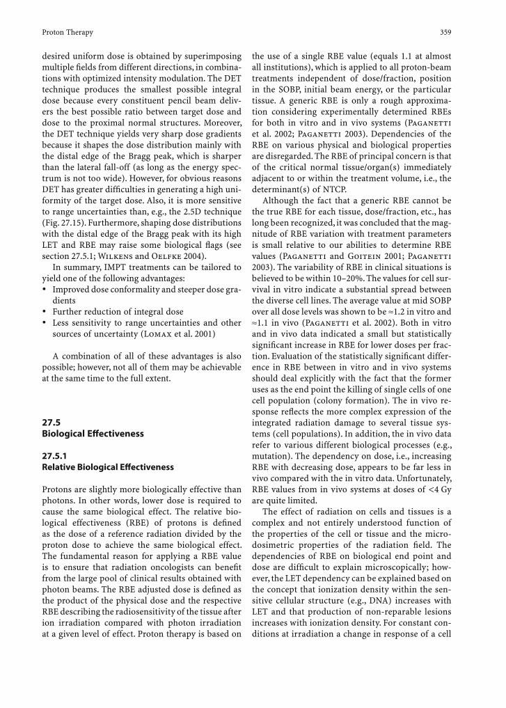
desired uniform dose is obtained by superimposing multiple fi elds from different directions, in combina-tions with optimized intensity modulation. The DET technique produces the smallest possible integral dose because every constituent pencil beam deliv-ers the best possible ratio between target dose and dose to the proximal normal structures. Moreover, the DET technique yields very sharp dose gradients because it shapes the dose distribution mainly with the distal edge of the Bragg peak, which is sharper than the lateral fall-off (as long as the energy spec-trum is not too wide). However, for obvious reasons DET has greater diffi culties in generating a high uni-formity of the target dose. Also, it is more sensitive to range uncertainties than, e.g., the 2.5D technique (Fig. 27.15). Furthermore, shaping dose distributions with the distal edge of the Bragg peak with its high LET and RBE may raise some biological fl ags (see section 27.5.1; Wilkens and Oelfke 2004).

In summary, IMPT treatments can be tailored to yield one of the following advantages:• Improved dose conformality and steeper dose gra-

dients• Further reduction of integral dose• Less sensitivity to range uncertainties and other

sources of uncertainty (Lomax et al. 2001)

A combination of all of these advantages is also possible; however, not all of them may be achievable at the same time to the full extent.

27.5 Biological Eff ectiveness

27.5.1 Relative Biological Eff ectiveness

Protons are slightly more biologically effective than photons. In other words, lower dose is required to cause the same biological effect. The relative bio-logical effectiveness (RBE) of protons is defi ned as the dose of a reference radiation divided by the proton dose to achieve the same biological effect. The fundamental reason for applying a RBE value is to ensure that radiation oncologists can benefi t from the large pool of clinical results obtained with photon beams. The RBE adjusted dose is defi ned as the product of the physical dose and the respective RBE describing the radiosensitivity of the tissue after ion irradiation compared with photon irradiation at a given level of effect. Proton therapy is based on

the use of a single RBE value (equals 1.1 at almost all institutions), which is applied to all proton-beam treatments independent of dose/fraction, position in the SOBP, initial beam energy, or the particular tissue. A generic RBE is only a rough approxima-tion considering experimentally determined RBEs for both in vitro and in vivo systems (Paganetti et al. 2002; Paganetti 2003). Dependencies of the RBE on various physical and biological properties are disregarded. The RBE of principal concern is that of the critical normal tissue/organ(s) immediately adjacent to or within the treatment volume, i.e., the determinant(s) of NTCP.

Although the fact that a generic RBE cannot be the true RBE for each tissue, dose/fraction, etc., has long been recognized, it was concluded that the mag-nitude of RBE variation with treatment parameters is small relative to our abilities to determine RBE values (Paganetti and Goitein 2001; Paganetti 2003). The variability of RBE in clinical situations is believed to be within 10–20%. The values for cell sur-vival in vitro indicate a substantial spread between the diverse cell lines. The average value at mid SOBP over all dose levels was shown to be ≈1.2 in vitro and ≈1.1 in vivo (Paganetti et al. 2002). Both in vitro and in vivo data indicated a small but statistically signifi cant increase in RBE for lower doses per frac-tion. Evaluation of the statistically signifi cant differ-ence in RBE between in vitro and in vivo systems should deal explicitly with the fact that the former uses as the end point the killing of single cells of one cell population (colony formation). The in vivo re-sponse refl ects the more complex expression of the integrated radiation damage to several tissue sys-tems (cell populations). In addition, the in vivo data refer to various different biological processes (e.g., mutation). The dependency on dose, i.e., increasing RBE with decreasing dose, appears to be far less in vivo compared with the in vitro data. Unfortunately, RBE values from in vivo systems at doses of <4 Gy are quite limited.

The effect of radiation on cells and tissues is a complex and not entirely understood function of the properties of the cell or tissue and the micro-dosimetric properties of the radiation fi eld. The dependencies of RBE on biological end point and dose are diffi cult to explain microscopically; how-ever, the LET dependency can be explained based on the concept that ionization density within the sen-sitive cellular structure (e.g., DNA) increases with LET and that production of non-reparable lesions increases with ionization density. For constant con-ditions at irradiation a change in response of a cell

Proton Therapy 359

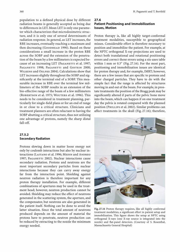
population to a defi ned physical dose by different radiation beams is generally accepted as being due to differences in LET. Mean LET is only one parame-ter which characterizes that microdosimetric struc-ture, and it is only one of several determinants of radiation response. In general, as LET increases, the RBE increases, eventually reaching a maximum and then decreasing (Goodhead 1990). Based on these considerations a small increase in the proton RBE across the SOBP and the extension of the penetra-tion of the beam by a few millimeters is expected be-cause of an increasing LET (Paganetti et al. 1997; Paganetti 1998; Paganetti and Goitein 2000; Wilkens and Oelfke 2004). Calculations show that LET increases slightly throughout the SOBP and sig-nifi cantly at the terminal end of a SOBP. This mea-surable increase in RBE over the terminal few mil-limeters of the SOBP results in an extension of the bio-effective range of the beam of a few millimeters (Robertson et al. 1975; Wouters et al. 1996). This needs to be considered in treatment planning, par-ticularly for single-fi eld plans or for an end of range in or close to a critical structure. Clinicians and treatment planners are often reluctant to having the SOBP abutting a critical structure, thus not utilizing one advantage of protons, namely the sharp distal fall-off.

27.5.2 Secondary Radiation

Protons slowing down in matter loose energy not only by coulomb interactions but also by nuclear in-teractions (Laitano et al. 1996; Medin and Andreo 1997; Paganetti 2002). Nuclear interactions cause secondary radiation. Protons and neutrons are the most important secondary particles from nuclear interactions because they can carry away energy far from the interaction point. Shielding against neutron radiation is therefore important for any proton therapy installation. For example, different combinations of apertures may be used in the treat-ment head; however, neutron production cannot be avoided. Shielding may reduce the effect of neutrons generated in the scattering system, the aperture, and the compensator, but neutrons are also generated in the patient itself. Nothing can be done to avoid the latter situation. Since the total amount of neutrons produced depends on the amount of material the protons have to penetrate, neutron production can be reduced by extracting to the nozzle the minimum energy needed.

27.6 Patient Positioning and Immobilization Issues, Motion

Proton therapy is, like all highly target-conformal treatment modalities, susceptible to geographical misses. Considerable effort is therefore necessary to position and immobilize the patient. For example, at the NPTC orthogonal X-ray projections are used to detect both translational and rotational positioning errors and correct those errors using a six-axes table within 1 mm or 0.5° (Fig. 27.16). For the most part, positioning and immobilization issues are identical for proton therapy and, for example, IMRT; however, there are a few issues that are specifi c to protons and other charged particles. They have to do with the simple fact that the range is affected by structures moving in and out of the beam. For example, in pros-tate treatments the position of the Bragg peak may be signifi cantly altered if parts of the pelvic bone move into the beam, which can happen if on one treatment day the pelvis is rotated compared with the planned position (Phillips et al. 2002). Similar problems can affect treatments in the skull (Fig. 27.16); therefore,

Fig. 27.16 Proton therapy requires, like all highly conformal treatment modalities, a signifi cant effort in patient setup and immobilization. This fi gure shows the setup at NPTC using orthogonal X-rays (one X-ray source is integrated into the nozzle) and fl at-panel detectors. (Courtesy of S. Rosenthal, Massachusetts General Hospital)

H. Paganetti and T. Bortfeld360

in particle therapy it is not only important to ensure that the target volume is always at the same posi-tion, but the surrounding structures and especially bony structures should also be at their planned po-sition. The detrimental effect of misalignments can be mitigated to some degree in treatment planning. A common approach in passive scattering proton therapy is to “smear” (thin) the range compensator such that target coverage is ensured even if the posi-tion is slightly off; however, this will push the dose into the normal tissues distal to the target volume, and the smearing radius is therefore limited to about 3 mm. Bigger errors cannot be compensated with this method.

Besides alignment errors, proton (and charged particle) therapy is also uniquely affected by internal organ motion, especially in the case of lung tumors. The dose distribution is deformed by the motion of the tumor in the low-density lung tissue. Unless methods such as gating (Minohara et al. 2000) are used to “freeze” the motion, this effect must be care-fully considered at treatment planning stage. This can be done (Moyers et al. 2001), but it is fair to say that the proton treatments of lung tumors have not yet fully come of age.

References

Archambeau JO, Slater JD, Slater JM, Tangeman R (1992) Role for proton beam irradiation in treatment of pediatric CNS malignancies. Int J Radiat Oncol Biol Phys 22:287–294

Benk V, Liebsch NJ, Munzenrider JE, Efi rd J, McManus P, Suit H (1995) Base of skull and cervical spine chordomas in chil-dren treated by high-dose irradiation. Int J Radiat Oncol Biol Phys 31:577–558

Blosser H, Bailey J, Burleigh R, Johnson D, Kashy E, Kuo T, Marti F, Vincent J, Zeller A, Blosser E, Blosser G, Maughan R, Power W, Wagner J (1989) Superconducting cyclotron for medical applications. IEEE Trans Magn 25:1746–1754

Bortfeld T, Jokivarsi K, Goitein M, Kung J, Jiang SB (2002) Effects of intra-fraction motion on IMRT dose delivery: statistical analysis and simulation. Phys Med Biol 47:2303–2320

Bussiere MR, Adams JA (2003) Treatment planning for con-formal proton radiation therapy. Technol Cancer Res Treat 2:389–399

Chu WT, Ludewigt BA, Renner TR (1993) Instrumentation for treatment of cancer using proton and light-ion beams. Rev Sci Instrum 64:2055–2122

Coutrakon G, Slater JM, Ghebremedhin A (1999) Design con-siderations for medical proton accelerators. Proc 1999 Par-ticle Accelerator Conference, New York, pp 11–15

Cozzi L, Fogliata A, Lomax A, Bolsi A (2001) A treatment plan-ning comparison of 3D conformal therapy, intensity mod-ulated photon therapy and proton therapy for treatment

of advanced head and neck tumours. Radiother Oncol 61:287–297

Deasy JO, Shepard DM, Mackie TR (1997) Distal edge tracking: a proposed delivery method for conformal proton therapy using intensity modulation. In: Leavitt DD, Starkschall G (eds) XIIth International Conference on the Use of Com-puters in Radiation Therapy. Medical Physics Publishing, Madison, Wisconsin, pp 406–409

Delaney TF, Smith AR, Lomax A, Adams J, Loeffl er JS (2003) Proton beam radiation therapy. Cancer Prin Pract Oncol 17:1–10

Flanz J, Durlacher S, Goitein M, Levine A, Reardon P, Smith A (1995) Overview of the MGH-Northeast Proton Therapy Center plans and progress. Nucl Instrum Methods Phys Res B 99:830–834

Fuss M, Hug EB, Schaefer RA, Nevinny-Stickel M, Miller DW, Slater JM, Slater JD (1999) Proton radiation therapy (PRT) for pediatric optic pathway gliomas: comparison with 3D planned conventional photons and a standard photon tech-nique. Int J Radiat Oncol Biol Phys 45:1117–1126

Fuss M, Poljanc K, Miller DW, Archambeau JO, Slater JM, Slater JD, Hug EB (2000) Normal tissue complication probability (NTCP) calculations as a means to compare proton and photon plans and evaluation of clinical appropriateness of calculated values. Int J Cancer 90:351–358

Goitein M, Jermann M (2003) The relative costs of proton and X-ray radiation therapy. Clin Oncol 15:S37–S50

Goitein M, Miller T (1983) Planning proton therapy of the eye. Med Phys 10:275–283

Goodhead DT (1990) Radiation effects in living cells. Can J Phys 68:872–886

Grusell E, Montelius A, Brahme A, Rikner G, Russell K (1994) A general solution to charged particle beam fl attening using an optimized dual-scattering-foil technique, with applica-tion to proton therapy beams. Phys Med Biol 39:2201–2216

Hara I, Murakami M, Kagawa K, Sugimura K, Kamidono S, Hishikawa Y, Abe M (2004) Experience with conformal proton therapy for early prostate cancer. Am J Clin Oncol 27:323–327

Harsh G, Loeffl er JS, Thornton A, Smith A, Bussiere M, Chap-man PH (1999) Stereotactic proton radiosurgery. Neuro-surg Clin North Am 10:243–256

Hong L, Goitein M, Bucciolini M, Comiskey R, Gottschalk B, Rosenthal S, Serago C, Urie M (1996) A pencil beam algo-rithm for proton dose calculations. Phys Med Biol 41:1305–1330

Hug EB, Slater JD (1999) Proton radiation therapy for pedi-atric malignancies: status report. Strahlenther Onkol 175 (Suppl) 2:89–91

Hug EB, Fitzek MM, Liebsch NJ, Munzenrider JE (1995) Locally challenging osteo- and chondrogenic tumors of the axial skeleton: results of combined proton and photon radiation therapy using three-dimensional treatment planning. Int J Radiat Oncol Biol Phys 31:467–476

Hug EB, Devries A, Thornton AF, Munzenrider JE, Pardo FS, Hedley-Whyte ET, Bussiere MR, Ojemann R (2000) Man-agement of atypical and malignant meningiomas: role of high-dose, 3D-conformal radiation therapy. J Neuro-Oncol 48:151–160

Isacsson U, Montelius A, Jung B, Glimelius B (1996) Com-parative treatment planning between proton and X-ray therapy in locally advanced rectal cancer. Radiother Oncol 41:263–272

Proton Therapy 361

Isacsson U, Hagberg H, Johansson K-A, Montelius A, Jung B, Glimelius B (1997) Potential advantages of protons over conventional radiation beams for paraspinal tumours. Radiother Oncol 45:63–70

Isacsson U, Lennernäs B, Grusell E, Jung B, Montelius A, Glime-lius B (1998) Comparative treatment planning between proton and X-ray therapy in esophageal cancer. Int J Radiat Oncol Biol Phys 41:441–450

Jiang H, Paganetti H (2004) Adaptation of GEANT4 to Monte Carlo dose calculations based on CT data. Med Phys 31:2811–2818

Kanai T, Kawachi K, Kumamoto Y, Ogawa H, Yamada T, Mat-suzawa H, Inada T (1980) Spot scanning system for proton radiotherapy. Med Phys 7:365–369

Koehler AM, Schneider RJ, Sisterson JM (1975) Range modu-lators for protons and heavy ions. Nucl Instrum Methods 131:437–440

Koehler AM, Schneider RJ, Sisterson JM (1977) Flattening of proton dose distributions for large-fi eld radiotherapy. Med Phys 4:297–301

Kraft G (2000) Tumortherapy with ion beams. Nucl Instrum Methods Phys Res A 454:1–10

Laitano RF, Rosetti M, Frisoni M (1996) Effects of nuclear interactions on energy and stopping power in proton beam dosimetry. Nucl Instrum Methods A 376:466–476

Lee M, Wynne C, Webb S, Nahum AE, Dearnaley D (1994) A comparison of proton and megavoltage X-ray treatment planning for prostate cancer. Radiother Oncol 33:239–253

Levin CV (1992) Potential for gain in the use of proton beam boost to the para-aortic lymph nodes in carcinoma of the cervix. Int J Radiat Oncol Biol Phys 22:355–359

Lin R, Hug EB, Schaefer RA, Miller DW, Slater JM, Slater JD (2000) Conformal proton radiation therapy of the posterior fossa: a study comparing protons with three-dimensional planned photons in limiting dose to auditory structures. Int J Radiat Oncol Biol Phys 48:1219–1226

Lomax A (1999) Intensity modulation methods for proton radiotherapy. Phys Med Biol 44:185–205

Lomax AJ, Bortfeld T, Goitein G, Debus J, Dykstra C, Tercier P-A, Coucke PA, Mirimanoff RO (1999) A treatment plan-ning inter-comparison of proton and intensity modulated photon radiotherapy. Radiother Oncol 51:257–271

Lomax AJ, Boehringer T, Coray A, Egger E, Goitein G, Gross-mann M, Juelke P, Lin S, Pedroni E, Rohrer B, Roser W, Rossi B, Siegenthaler B, Stadelmann O, Stauble H, Vetter C, Wisser L (2001) Intensity modulated proton therapy: a clinical example. Med Phys 28:317–324

Lomax AJ, Cella L, Weber D, Kurtz JM, Miralbell R (2003a) Potential role of intensity-modulated photons and protons in the treatment of the breast and regional nodes. Int J Radiat Oncol Biol Phys 55:785–792

Lomax AJ, Goitein M, Adams J (2003b) Intensity modulation in radiotherapy: photons versus protons in the paranasal sinus. Radiother Oncol 66:11–18

McAllister B, Archambeau JO, Nguyen MC, Slater JD, Loredo L, Schulte R, Alvarez O, Bedros AA, Kaleita T, Moyers M, Miller D, Slater JM (1997) Proton therapy for pediat-ric cranial tumors: preliminary report on treatment and disease-related morbidities. Int J Radiat Oncol Biol Phys 39:455–460

Medin J, Andreo P (1997) Monte Carlo calculated stopping-power ratios, water/air, for clinical proton dosimetry (50–250 MeV). Phys Med Biol 42:89–105

Minohara S, Kanai T, Endo M, Noda K, Kanazawa M (2000) Respiratory gated irradiation system for heavy-ion radio-therapy. Int J Radiat Oncol Biol Phys 47:1097–1103

Miralbell R, Crowell C, Suit HD (1992) Potential improvement of three dimension treatment planning and proton therapy in the outcome of maxillary sinus cancer. Int J Radiat Oncol Biol Phys 22:305–310

Miralbell R, Lomax A, Russo M (1997) Potential role of proton therapy in the treatment of pediatric medulloblastoma/primitive neuro-ectodermal tumors: spinal theca irradia-tion. Int J Radiat Oncol Biol Phys 38:805–811

Moyers MF, Miller DW, Bush DA, Slater JD (2001) Methodolo-gies and tools for proton beam design for lung tumors. Int J Radiat Oncol Biol Phys 49:1429–1438

Niemierko A, Urie M, Goitein M (1992) Optimization of 3D radiation therapy with both physical and biological end points and constraints. Int J Radiat Oncol Biol Phys 23:99–108

Nowakowski VA, Castro JR, Petti PL, Collier JM, Daftari I, Ahn D, Gauger G, Gutin P, Linstadt DE, Phillips TL (1992) Charged particle radiotherapy of paraspinal tumors. Int J Radiat Oncol Biol Phys 22:295–303

Oelfke U, Bortfeld T (2001) Inverse planning for photon and proton beams. Med Dosim 26:113–124

Paganetti H (1998) Calculation of the spatial variation of rela-tive biological effectiveness in a therapeutic proton fi eld for eye treatment. Phys Med Biol 43:2147–2157

Paganetti H (2002) Nuclear interactions in proton therapy: dose and relative biological effect distributions originat-ing from primary and secondary particles. Phys Med Biol 47:747–764

Paganetti H (2003) Signifi cance and implementation of RBE variations in proton beam therapy. Technol Cancer Res Treatment 2:413–426

Paganetti H, Goitein M (2000) Radiobiological signifi cance of beam line dependent proton energy distributions in a spread-out Bragg peak. Med Phys 27:1119–1126

Paganetti H, Goitein M (2001) Biophysical modeling of proton radiation effects based on amorphous track models. Int J Radiat Biol 77:911–928

Paganetti H, Olko P, Kobus H, Becker R, Schmitz T, Waligorski MPR, Filges D, Mueller-Gaertner HW (1997) Calculation of RBE for proton beams using biological weighting func-tions. Int J Radiat Oncol Biol Phys 37:719–729

Paganetti H, Niemierko A, Ancukiewicz M, Gerweck LE, Loef-fl er JS, Goitein M, Suit HD (2002) Relative biological effec-tiveness (RBE) values for proton beam therapy. Int J Radiat Oncol Biol Phys 53:407–421

Paganetti H, Jiang H, Adams JA, Chen GT, Rietzel E (2004a) Monte Carlo simulations with time-dependent geometries to investigate organ motion with high temporal resolution. Int J Radiat Oncol Biol Phys 60:942–950

Paganetti H, Jiang H, Lee S-Y, Kooy H (2004b) Accurate Monte Carlo for nozzle design, commissioning, and quality assur-ance in proton therapy. Med Phys 31:2107–2118

Pawlicki T, Ma C-MC (2001) Monte Carlo simulation for MLC-based intensity-modulated radiotherapy. Med Dosim 26:157–168

Pedroni E, Bacher R, Blattmann H, Boehringer T, Coray A, Lomax A, Lin S, Munkel G, Scheib S, Schneider U, Tourovsky A (1995) The 200-MeV proton therapy project at the Paul Scherrer Institute: conceptual design and practical realiza-tion. Med Phys 22:37–53

H. Paganetti and T. Bortfeld362

Phillips MH, Pedroni E, Blattmann H, Boehringer T, Coray A, Scheib S (1992) Effects of respiratory motion on dose uniformity with a charged particle scanning method. Phys Med Biol 37:223–234

Phillips BL, Jiroutek MR, Tracton G, Elfervig M, Muller KE, Chaney EL (2002) Thresholds for human detection of patient setup errors in digitally reconstructed portal images of prostate fi elds. Int J Radiat Oncol Biol Phys 54:270–277

Robertson JB, Williams JR, Schmidt RA, Little JB, Flynn DF, Suit HD (1975) Radiobiological studies of a high-energy modulated proton beam utilizing cultured mammalian cells. Cancer 35:1664–1677

Rosenberg AE, Nielsen GP, Keel SB, Renard LG, Fitzek MM, Munzenrider JE, Liebsch NJ (1999) Chondrosarcoma of the base of the skull: a clinicopathologic study of 200 cases with emphasis on its distinction from chordoma. Am J Surg Pathol 23:1370–1378

Shioyama Y, Tokuuye K, Okumura T, Kagei K, Sugahara S, Ohara K, Akine Y, Ishikawa S, Satoh H, Sekizawa K (2003) Clinical evaluation of proton radiotherapy for non-small-cell lung cancer. Int J Radiat Oncol Biol Phys 56:7–13

Sisterson JM (2004) Particles Newsletter. http://ptcog.mgh.harvard.edu

Sisterson JM, Urie MM, Koehler AM, Goitein M (1989) Distal penetration of proton beams: the effects of air gaps between compensating bolus and patient. Phys Med Biol 34:1309–1315

Slater JD, Slater JM, Wahlen S (1992a) The potential for proton beam therapy in locally advanced carcinoma of the cervix. Int J Radiat Oncol Biol Phys 22:343–347

Slater JM, Slater JD, Archambeau JO (1992b) Carcinoma of the tonsillar region: potential for use of proton beam therapy. Int J Radiat Oncol Biol Phys 22:311–319

Slater JD, Rossi CJJ, Yonemoto LT, Bush DA, Jabola BR, Levy RP, Grove RI, Preston W, Slater JM (2004) Proton therapy for prostate cancer: the initial Loma Linda University experi-ence. Int J Radiat Oncol Biol Phys 59:348–352

Smit BM (1992) Prospects for proton therapy in carcinoma of the cervix. Int J Radiat Oncol Biol Phys 22:349–353

Tatsuzaki H, Urie MM, Linggood R (1992a) Comparative treat-ment planning: proton vs X-ray beams against glioblastoma multiforme. Int J Radiat Oncol Biol Phys 22:265–273

Tatsuzaki H, Urie MM, Willett CG (1992b) 3-D comparative

study of proton vs X-ray radiation therapy for rectal cancer. Int J Radiat Oncol Biol Phys 22:369–374

Terahara A, Niemierko A, Goitein M, Finkelstein D, Hug E, Liebsch N, O’Farrell D, Lyons S, Munzenrider J (1999) Anal-ysis of the relationship between tumor dose inhomogene-ity and local control in patients with skull base chordoma. Int J Radiat Oncol Biol Phys 45:351–358

Thornton A, Fitzek M, Varvares M, Adams J, Rosenthal S, Pol-lock S, Jackson M, Pilch B, Joseph M (1998) Accelerated hyperfractionated proton/photon irradiation for advanced paranasal sinus cancer. Results of a perspective phase I–II study. Int J Radiat Oncol Biol Phys 42 (Suppl):222

Tobias CA, Lawrence JH, Born JL, McCombs R, Roberts JE, Anger HO, Low-Beer BVA, Huggins C (1958) Pituitary irradiation with high energy proton beams: a preliminary report. Cancer Res 18:121–134

Trofi mov A, Bortfeld T (2003) Optimization of beam param-eters and treatment planning for intensity modulated proton therapy. Technol Cancer Res Treatment 2:437–444

Wambersie A, Gregoire V, Brucher J-M (1992) Potential clinical gain of proton (and heavy ion) beams for brain tumors in children. Int J Radiat Oncol Biol Phys 22:275–286

Weber DC, Trofi mov AV, Delaney TF, Bortfeld T (2004) A treat-ment plan comparison of intensity modulated photon and proton therapy for paraspinal sarcomas. Int J Radiat Oncol Biol Phys 58:1596–1606

Wenkel E, Thornton AF, Finkelstein D, Adams J, Lyons S, Monte S de la, Ojeman RG, Munzenrider JE (2000) Benign menin-gioma: partially resected, biopsied, and recurrent intra-cranial tumors treated with combined proton and photon radiotherapy. Int J Radiat Oncol Biol Phys 48:1363–1370

Wilkens JJ, Oelfke U (2004) A phenomenological model for the relative biological effectiveness in therapeutic proton beams. Phys Med Biol 49:2811–2825

Wilson RR (1946) Radiological use of fast protons. Radiology 47:487–491

Wouters BG, Lam GKY, Oelfke U, Gardey K, Durand RE, Skars-gard LD (1996) RBE Measurement on the 70 MeV Proton Beam at TRIUMF using V79 cells and the high precision cell sorter assay. Radiat Res 146:159–170

Yeboah C, Sandison GA (2002) Optimized treatment planning for prostate cancer comparing IMPT, VHEET and 15 mV IMXT. Phys Med Biol 47:2247-2261

Proton Therapy 363

Heavy Ion Radiotherapy 365

28 Heavy Ion Radiotherapy

Oliver Jäkel

O. Jäkel, PhDAbteilung für Medizinische Physik in der Strahlentherapie, Deutsches Krebsforschungszentrum, Im Neuenheimer Feld 280, 69120 Heidelberg, Germany

28.1 Introduction

Within the past two decades not only photon ra-diotherapy has rapidly developed, but also particle therapy with protons as well as helium and carbon ions has gained increasing interest (Jäkel et al. 2003). The term “heavy ions” is used here for ions heavier than helium ions. The primary rationale for radio-therapy with heavy charged particles is the sharp increase of dose in a well-defi ned depth (Bragg peak) and the rapid dose fall-off beyond that maximum

(see Fig. 28.2). The ratio of Bragg peak dose vs dose in the entrance region is larger for heavy ions than for protons. Due to their larger mass, angular and energy straggling of the primary particles is becoming negli-gible for heavy ions as compared with protons or even helium ions. Heavy ions therefore offer an improved dose conformation as compared with photon and proton radiotherapy with better sparing of normal tissue structures close to the target. In addition, heavy ions exhibit a strong increase of the linear energy transfer (LET) in the Bragg peak as compared with the entrance region. The radiobiological advantage of high LET radiation in tumor therapy is well known from neutron therapy. Unlike in radiotherapy with neutron beams, in heavy ion radiotherapy the high LET region can also be conformed to the tumor.

Between 1977 and 1992, fi rst clinical experiences have been made, especially with helium and neon ions at the Lawrence Berkeley Laboratory and many encouraging results (especially in skull base tumors and paraspinal tumors) were achieved (Castro et al. 1994; Castro 1997).

The increasing effectiveness of ions with larger charge is shown in Fig. 28.1. Although helium ions are very similar to protons in their biological proper-ties, carbon or neon ions exhibit an increased rela-tive biological effectiveness (RBE) in the Bragg peak as compared with the entrance region (see Fig. 28.1). The RBE ratio (Bragg peak vs entrance region) is highest for carbon ions. For ions heavier than neon, the RBE in the entrance region is even higher than in the Bragg peak (like for argon).

Another disadvantage of very heavy ions for ra-diotherapy is the increase of nuclear fragmentation processes, which leads to a fragment tail in the depth dose distribution that extends beyond the Bragg peak (see Fig. 28.2).

Currently the availability of heavy ion radio-therapy is limited, as worldwide only three facilities offer carbon ion radiotherapy: two hospital-based facilities in Japan [Heavy Ion Medical Accelerator (HIMAC), Chiba; Hyogo Ion Beam Medical Center (HIBMC), Hyogo] and a physics research facility

CONTENTS

28.1 Introduction 36528.2 Treatment Techniques 36628.2.1 Beam Production and Beam Delivery Systems 36628.2.2 Beam Application Systems 36728.2.2.1 Passive Beam Shaping 36728.2.2.2 Active Beam Shaping 36728.2.3 Patient Positioning 36728.2.4 Treatment Planning 36828.2.4.1 TPS for Passive Beam Shaping 36828.2.4.2 TPS for Active Beam Shaping 36928.3 Existing and Planned Facilities 37028.3.1 The Bevalac Facility 37028.3.2 The HIMAC Facility 37028.3.3 The GSI Facility 37128.3.4 The HIBMC Facility 37128.3.5 New Facilities 37128.4 Clinical Application of Ion Beams 37228.4.1 Clinical Trials at Berkeley 37228.4.2 Clinical Trials and Routine Treatments at GSI 37328.4.3 Treatments at HIMAC 37428.5 Outlook 375 References 376

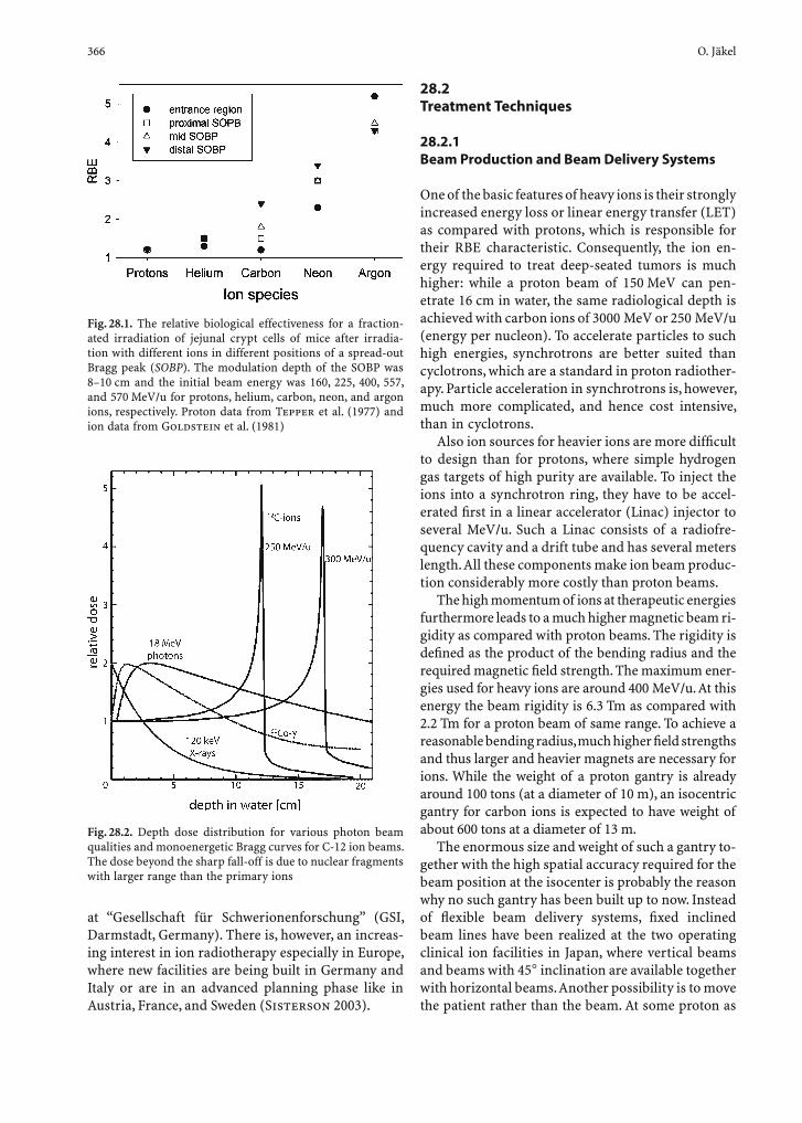
366 O. Jäkel

at “Gesellschaft für Schwerionenforschung” (GSI, Darmstadt, Germany). There is, however, an increas-ing interest in ion radiotherapy especially in Europe, where new facilities are being built in Germany and Italy or are in an advanced planning phase like in Austria, France, and Sweden (Sisterson 2003).

28.2 Treatment Techniques

28.2.1 Beam Production and Beam Delivery Systems

One of the basic features of heavy ions is their strongly increased energy loss or linear energy transfer (LET) as compared with protons, which is responsible for their RBE characteristic. Consequently, the ion en-ergy required to treat deep-seated tumors is much higher: while a proton beam of 150 MeV can pen-etrate 16 cm in water, the same radiological depth is achieved with carbon ions of 3000 MeV or 250 MeV/u (energy per nucleon). To accelerate particles to such high energies, synchrotrons are better suited than cyclotrons, which are a standard in proton radiother-apy. Particle acceleration in synchrotrons is, however, much more complicated, and hence cost intensive, than in cyclotrons.

Also ion sources for heavier ions are more diffi cult to design than for protons, where simple hydrogen gas targets of high purity are available. To inject the ions into a synchrotron ring, they have to be accel-erated fi rst in a linear accelerator (Linac) injector to several MeV/u. Such a Linac consists of a radiofre-quency cavity and a drift tube and has several meters length. All these components make ion beam produc-tion considerably more costly than proton beams.

The high momentum of ions at therapeutic energies furthermore leads to a much higher magnetic beam ri-gidity as compared with proton beams. The rigidity is defi ned as the product of the bending radius and the required magnetic fi eld strength. The maximum ener-gies used for heavy ions are around 400 MeV/u. At this energy the beam rigidity is 6.3 Tm as compared with 2.2 Tm for a proton beam of same range. To achieve a reasonable bending radius, much higher fi eld strengths and thus larger and heavier magnets are necessary for ions. While the weight of a proton gantry is already around 100 tons (at a diameter of 10 m), an isocentric gantry for carbon ions is expected to have weight of about 600 tons at a diameter of 13 m.

The enormous size and weight of such a gantry to-gether with the high spatial accuracy required for the beam position at the isocenter is probably the reason why no such gantry has been built up to now. Instead of fl exible beam delivery systems, fi xed inclined beam lines have been realized at the two operating clinical ion facilities in Japan, where vertical beams and beams with 45° inclination are available together with horizontal beams. Another possibility is to move the patient rather than the beam. At some proton as

Fig. 28.1. The relative biological effectiveness for a fraction-ated irradiation of jejunal crypt cells of mice after irradia-tion with different ions in different positions of a spread-out Bragg peak (SOBP). The modulation depth of the SOBP was 8–10 cm and the initial beam energy was 160, 225, 400, 557, and 570 MeV/u for protons, helium, carbon, neon, and argon ions, respectively. Proton data from Tepper et al. (1977) and ion data from Goldstein et al. (1981)

Fig. 28.2. Depth dose distribution for various photon beam qualities and monoenergetic Bragg curves for C-12 ion beams. The dose beyond the sharp fall-off is due to nuclear fragments with larger range than the primary ions

Heavy Ion Radiotherapy 367

well as heavy ion facilities, treatment chairs are avail-able or moulds that can be rotated (see patient posi-tioning for details).

It is noteworthy that size and weight of a gantry can be reduced by the use of superconducting mag-nets. The cryogenics involved, however, requires considerable space and is more delicate to handle in terms of stability and patient safety.

28.2.2 Beam Application Systems

There exist two principle methods to shape the beam and thus to tailor the dose to the target volume, which are described in the next sections.

28.2.2.1 Passive Beam Shaping

Passive beam shaping was the fi rst method to be de-veloped and still is most commonly used in proton and heavy ion therapy. In a fi rst step, the depth dose of the monoenergetic beam from the accelerator is modulated by a variable degrader. This degrader may be a rotating wheel with varying thickness or a wobbling plate with wedge-shaped engravings (ridge fi lter). In both cases the modulator is designed such that a predefi ned depth dose profi le results. To cover different depth modulations in tissue, several differ-ent modulators are available.

In order to move the modulated Bragg peak (or spread-out Bragg peak, SOBP) to the desired radio-logical depth, an additional range shifter is needed. It consists typically of a number of homogeneous plas-tic plates of different thickness, which can be moved into the beam.

Finally, the small-sized beam has to be spread out laterally to cover the whole target homogeneously. This is achieved either by a double scattering sys-tem, or by a magnetic wobbling system that moves the beam over a defi ned area (Fig. 28.3 schematically shows the design of a passive beam delivery system).

To adapt the dose individually for each patient, patient-specifi c hardware is necessary. Using a col-limator, the lateral extent of each treatment fi eld is adapted to the beams-eye view of the target volume. An additional compensator is used to account for tis-sue inhomogeneities and the curvature of the patient surface. The compensator is designed such that the distal end of the modulated Bragg peak matches the distal end of the target volume. In doing so, the depth dose profi le can only be shifted to smaller depths.

The passive beam-shaping technique for ions has three major disadvantages: fi rstly, the depth dose can only be tailored to the distal end of the target, but not to the proximal end. This is due to the fact that the com-pensator shifts the SOBP towards the entrance region. A considerable amount of the high-dose region (and high LET region) is therefore located in the normal tissue in front of the target volume, especially at the lateral fi eld borders. Secondly, the amount of material in the beam line is considerable, leading to an increase in nuclear fragments produced by nuclear interactions with the material of the beam modifi ers. These nuclear fragments have lower energies and lead to a higher LET and thus an increased biological effective dose of the beam already in the entrance region. A third aspect is the large number of patient-specifi c beam modifi ers which have to be manufactured (a compensator and a collimator for each treatment fi eld) and the necessity to produce a number of modulators which may have to be exchanged for different patients. It should be noted that also the use of Multileaf collimators for carbon ions in combination with a SOBP of variable depths has been proposed (Kanematsu et al. 2000), in order to achieve an improved sparing of normal tissue.

28.2.2.2 Active Beam Shaping

Another way of beam delivery is called active beam shaping. This systems takes advantage of the electric charge of ions, in order to produce a tightly focused

Fig. 28.3. Principle of the passive dose delivery system used for proton and ion beams. Shown is the incoming broadened beam that is modulated in depth. The variable range shifter has to shift the modulated depth dose to the desired depth, whereas collimator and compensator are patient-specifi c de-vices. The lines in the body represent the distal dose fall-off that can be shifted in depth with the range shifter

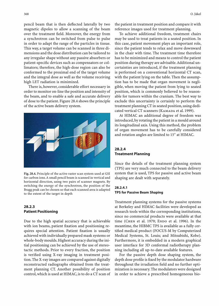
368 O. Jäkel

pencil beam that is then defl ected laterally by two magnetic dipoles to allow a scanning of the beam over the treatment fi eld. Moreover, the energy from a synchrotron can be switched from pulse to pulse in order to adapt the range of the particles in tissue. This way, a target volume can be scanned in three di-mensions and the dose distribution can be tailored to any irregular shape without any passive absorbers or patient-specifi c devices such as compensators or col-limators; therefore, the high-dose region can also be conformed to the proximal end of the target volume and the integral dose as well as the volume receiving high LET radiation is minimized.

There is, however, considerable effort necessary in order to monitor on-line the position and intensity of the beam, and to enable a safe and accurate delivery of dose to the patient. Figure 28.4 shows the principle of the active beam delivery system.

the patient in treatment position and compare it with reference images used for treatment planning.

To achieve additional freedom, treatment chairs may be used to treat patients in a seated position. In this case, patient movement plays an important role, since the patient tends to relax and move downward in the chair with time. The treatment time therefore has to be minimized and means to control the patient position during therapy are advisable. Additional un-certainties are introduced, if the treatment planning is performed on a conventional horizontal CT scan, with the patient lying on the table. Then the assump-tion has to be made that organ movement is negli-gible, when moving the patient from lying to seated position, which is commonly believed to be reason-able for tumors within the cranium. The best way to exclude this uncertainty is certainly to perform the treatment planning CT in seated position, using dedi-cated vertical CT scanners (Kamada et al. 1999).

At HIMAC an additional degree of freedom was introduced, by rotating the patient in a mould around its longitudinal axis. Using this method, the problem of organ movement has to be carefully considered and rotation angles are limited to 15° at HIMAC.

28.2.4 Treatment Planning

Since the details of the treatment planning system (TPS) are very much connected to the beam delivery system that is used, TPS for passive and active beam shaping are dealt with separately.

28.2.4.1 TPS for Passive Beam Shaping

Treatment planning systems for the passive systems at Berkeley and HIMAC facilities were developed as research tools within the corresponding institutions, since no commercial products were available at that time (Chen et al. 1979; Endo et al. 1996). In the meantime, the HIBMC TPS is available as a fully cer-tifi ed medical product (FOCUS-M by Computerized Medical Systems, St. Louis; and Mitsubishi, Kobe). Furthermore, it is embedded in a modern graphical user interface for 3D conformal radiotherapy plan-ning including all up-to-date available features.

For the passive depth dose shaping system, the depth dose profi le is fi xed by the modulator hardware throughout the irradiation fi eld and no further opti-mization is necessary. The modulators were designed in order to achieve a prescribed homogeneous bio-

Fig. 28.4. Principle of the active raster scan system used at GSI for carbon ions. A small pencil beam is scanned in vertical and horizontal direction, using two pairs of scanner magnets. By switching the energy of the synchrotron, the position of the Bragg peak can be chosen so that each scanned area is adapted to the extent of the target in depth

28.2.3 Patient Positioning

Due to the high spatial accuracy that is achievable with ion beams, patient fi xation and positioning re-quires special attention. Patient fi xation is usually achieved with individually prepared mask systems or whole-body moulds. Highest accuracy during the ini-tial positioning can be achieved by the use of stereo-tactic methods. Prior to every fraction, the position is verifi ed using X-ray imaging in treatment posi-tion. The X-ray images are compared against digitally reconstructed radiographs obtained from the treat-ment planning CT. Another possibility of position control, which is used at HIMAC, is to do a CT scan of

Heavy Ion Radiotherapy 369

logical effective dose for a single fi eld. The design of the modulators refl ects the fi xed dependence of the RBE with depth for a certain dose level.

Absorbed Dose Calculation

The algorithms to calculate absorbed dose for a pas-sive beam shaping system are very similar to those used in conventional photon therapy. The beam trans-port models are relatively simple, as lateral scattering of carbon or even neon ions is very small and the lateral penumbra of the primary beam is preserved almost completely in depth. The modeling of nuclear fragmentation is not a serious problem, because treat-ment planning can rely on measured depth dose data that include fragmentation. These measurements for the various depth modulators are performed in water and sum up the dose contribution of all fragments. The radiological depth of the beam in tissue is calcu-lated using an empirical relation between X-ray CT numbers and measured particle ranges (Minohara et al. 1993; Jäkel et al. 2001a, b).

Using this procedure, the design of necessary pa-tient-specifi c devices, such as bolus, compensators, and collimators, can be optimized by computer pro-grams. Similar to photon therapy, only relative val-ues of the absorbed dose may be used, because the absorbed dose scales with the number of monitor units.

Biological Modeling

The situation is more complicated for the calcula-tion of biological effective dose, because the relative biological effi ciency (RBE) of an ion beam in tissue depends on the underlying LET spectrum, the cell type, the dose level, and some other quantities. This problem was solved by a number of pragmatic steps and assumptions for passive beam delivery systems (Kanai et al. 1999).

The clinical RBE is replaced by an LET-dependent RBE for in vitro data under well-defi ned conditions and then linked to clinical data by an empirical fac-tor. At HIMAC, for example, the RBE value for the 10% survival level of human salivary gland (HSG) cells was chosen and then linked to the existing clini-cal data gained in fast neutron radiotherapy at the corresponding LET level (see also the chapter on “Biological models for treatment planning”).

The fractionation scheme and dose per fraction are kept fi xed and only one modulator yielding a cer-tain depth dose is used for each treatment fi eld. This is possible, as several fi elds of a treatment plan are

applied on different treatment days; thus, the treat-ment fi elds can be considered to be independent and the effective dose values can simply be added up.

Under these conditions, the resulting RBE can be approximated to be only a function of depth. If this function is determined, a corresponding ridge fi lter can be designed in such a way that the resulting depth dose curve leads to a constant biological effective dose. Consequently, no further biological modeling or optimization is necessary once the ridge fi lters are designed.

28.2.4.2 TPS for Active Beam Shaping

For an active beam shaping system for ions a research TPS was developed for the GSI facility. The system is a combination of a versatile graphical user interface for radiotherapy planning, called Virtuos (Virtual ra-diotherapy simulator; Bendl et al. 1993), and a pro-gram called TRiP (Treatment planning for particles), which handles all ion-specifi c tasks (Krämer and Scholz 2000; Krämer et al. 2000). Virtuos features most tools used in modern radiotherapy planning, whereas TRiP handles the optimization of absorbed as well as biological effective dose and the optimiza-tion of the machine control data.

The introduction of a 3D scanning system has some important consequences for the TPS.

A modulator for passive beam shaping is designed to achieve a prescribed homogeneous biological ef-fective dose for a single fi eld. A 3D scanning system, however, can produce nearly arbitrary shapes of the SOBP. The shape of the SOBP therefore has to be op-timized separately for every scan point in the irradia-tion fi eld.

The resulting new demands on the TPS are:• The beam intensity of every scan point at every

energy has to be optimized separately to obtain a homogeneous biological effect.

• As the system is able to apply any complicated inhomogeneous dose distribution, the capability for intensity-modulated radiotherapy with ions should be taken into account.

• All fi elds of a treatment plan are applied on the same day to avoid uncertainties in the resulting dose due to setup errors.

• The dose per fraction should be variable for every patient.

• The scanner control data (energy, beam position, particle number at every beam spot) have to be optimized for each fi eld of every patient.

• An RBE model has to be implemented, which allows

370 O. Jäkel

the calculation of a local RBE at every point in the patient depending on the spectrum of particles at this point. In addition, dedicated quality assurance measures for such a novel TPS have to be devel-oped (Jäkel et al. 2000, Krämer et al. 2003).

Absorbed Dose Calculation

The dose calculation for active beam shaping sys-tems is very similar to the pencil-beam models used for conventional photon therapy and also relies on measured data like for the passive systems. Instead of the measured depth dose data for the SOBPs resulting from the modulators, data for the single energies are needed. If the applied dose is variable, it is necessary to base the calculation of absorbed dose on absolute particle numbers rather than on relative values. For the calculation of absorbed dose, the integral data including all fragments are suffi cient.

Before the actual dose calculation starts, the tar-get volume is divided into slices of equal radiological depth. (Here the same empirical methods of range calculation as for passive systems are used.) Each slice then corresponds to the range of ions at a certain energy of the accelerator. The scan positions of the raster scanner are then defi ned as a quadratic grid for each energy. In the last step, the particle number at each scan point is optimized iteratively until a pre-defi ned dose at each point is reached.

Biological Modeling

To fulfi ll the demands of an active beam delivery on the TPS concerning the biological effectiveness, a more sophisticated biological model is needed. Such a model was developed, e.g., at GSI (Scholz et al. 1997). Its main idea is to transfer known cell survival data for photons to ions, assuming that the difference in biological effi ciency arises only from a different pattern of local dose deposition along the primary beam (see also the chapter on “Biological models for treatment planning”).

The model takes into account the different energy deposition patterns of different ions and is thus able to model the biological effect resulting from these ions. An important prerequisite for this is, however, the detailed knowledge of the number of fragments produced as well as their energy spectrum. The cal-culated RBE shows a dependence on the dose level and cell type, if the underlying photon survival data for this respective cell type are known.

The model allows the optimization of a prescribed biological effective dose within the target volume

(Krämer and Scholz 2000; Jäkel et al. 2001b) us-ing the same iterative optimization algorithm as for the absorbed dose. At each iteration step, however, the RBE has to be calculated anew, as it is dependent on the particle number (or dose level). Since this includes the knowledge of the complete spectrum of fragments, the optimization is time-consuming. Again, it has to be pointed out that the dose depen-dence of the RBE demands the use of absolute dose values during optimization.

28.3 Existing and Planned Facilities

28.3.1 The Bevalac Facility

Pioneering work in the fi eld of radiotherapy with heavy ions was performed at the University of California, Berkeley. The Bevalac provided the scien-tifi c and technological basis for many of the current developments in the fi eld of ion radiotherapy. Between 1977 and 1992, 433 patients have been treated here in total with ions heavier than helium. The majority of patients received neon ion treatments, although some patients were also treated with carbon, silicon, and argon beams (Castro and Lawrence 1978; Castro et al. 1994).

At the Bevalac, two treatment rooms, both equipped with a fi xed horizontal beam line, were available. The majority of the patients were treated in a sitting posi-tion. For treatment planning, a CT scanner was modi-fi ed to scan patients in a seated position.

The modulation of depth dose was performed using a fi xed accelerator energy and passive range modulators, like ridge fi lters and patient-specifi c compensators. The lateral width of the beam was produced using a double scattering system and was improved to a beam wobbling system in the 1980s. Patient-specifi c fi eld collimators were used to con-fi ne the beam to the target volume. A magnetic beam scanning system was installed in combination with a passive range modulator, which was used, however, for the treatment of a single patient only.

28.3.2 The HIMAC Facility

The HIMAC started its clinical operation in Chiba, Japan, in 1994. As of February 2002, 1187 patients

Heavy Ion Radiotherapy 371

have been treated with carbon ions (Tsujii et al. 2002). Two redundant synchrotrons deliver carbon ion beams at energies of 290, 350, and 400 MeV/u.

Patients are treated in three different treatment rooms, which are equipped with a vertical beam line, a horizontal beam line, and the third with a vertical and a horizontal beam line, respectively.

For more fl exibility, treatment chairs are used additionally to conventional treatment couches. In addition, a tub-like system may be mounted on the treatment table to allow a small angle rotation of the patient around the longitudinal axis. For treatments in seated position, special horizontal CT scanners are available for treatment planning (Kamada et al. 1999).

The beam delivery uses passive range modula-tion by bar ridge fi lters to achieve a fi xed modulation depth. The lateral fi eld width is obtained by a wobbler system and beam shaping is achieved by patient-spe-cifi c collimators (Kanai et al. 1999).

28.3.3 The GSI Facility

At the research laboratory GSI in Darmstadt (Germany), a therapy unit began its clinical opera-tion in 1997 (Eickhoff et al. 1999; Debus et al. 2000). As of spring 2004, more than 220 patients have been treated with carbon ions. Only one treatment room is available that is equipped with a treatment couch. An additional treatment chair will come into clinical operation in the near future.

The beam delivery system is completely active and allows 3D scanning of arbitrarily shaped vol-umes with a spatial resolution of 2 mm in all three directions. Using a magnetic defl ection system, the intensity-controlled raster scanner can deliver a monoenergetic pencil beam over an arbitrarily shaped area (Haberer et al. 1993). To do so, a beam of 4–10 mm full-width half-maximum is scanned over a regular grid of points with typically 2- to 3-mm spacing. After completion of a scan, the accel-erator energy can be switched from pulse to pulse and another scan can be performed with a different radiological depth. In total, 252 accelerator energies are available.

A feedback loop from the intensity control moves the beam to the next beam spot, when a predefi ned number of particles is reached. An on-line monitor-ing of the beam position and a feedback loop to the scanner is used to keep the beam extremely stable at each scan spot.

28.3.4 The HIBMC Facility

The Hyogo Ion Beam Medical Center (HIBMC) started operation with protons in 2001 and with carbon ions in 2002 at Harima Science Garden City, Japan. It is the fi rst facility offering carbon ion and proton treatment at the same facility. As of mid-2002, 28 patients have received carbon ion therapy (Itano et al. 2003). Six therapy rooms are available with seven treatment ports. Three rooms are dedicated to carbon ion beams: one with a vertical beam line; one with a horizontal; and one with a 45° oblique beam line, respectively. Two proton treatment rooms are equipped with commercially designed gantries. The beam delivery system is based on the HIMAC system.

28.3.5 New Facilities

There is currently an increasing interest in heavy ion radiotherapy especially in Europe and Asia (Sisterson 2003). There are proposals for hospital based heavy ion facilities in Lyon (France), Pavia (Italy), Stockholm (Sweden), and Vienna (Austria). Only two facilities (in Italy and Germany), however, have by now reached the phase of construction or call for tenders. In Lanzhou (China) an existing heavy ion research facility is preparing for clinical patient treatments with ions. The therapy facility will be in-stalled within the environment of a research labo-ratory, similar to the GSI facility. It features only a horizontal beam line.

The Italian project is driven by the CNAO (“Centro Nazionale Adroterapia”) and will set up the facility in Pavia near Milan. It will exhibit a synchrotron of about 25 m diameter that is capable of accelerating protons and carbon ions up to energies of 400 MeV/u. It features three treatment rooms equipped with horizontal beam lines, one of them with an addi-tional proton gantry. Beam scanning will be available at all beam lines. The construction of this fi rst phase should start at the beginning of 2004 and the fi rst pa-tient is planned to be treated at the end of 2007. Then, in a second project phase, the construction of two ad-ditional treatment rooms equipped with supercon-ducting isocentric ion gantries will take place.

The currently most ambitious and advanced project is the Heavy Ion Therapy accelerator (HIT) which will be installed at the Heidelberg University Hospital (Heeg et al. 2004; Eickhoff et al. 1998). The

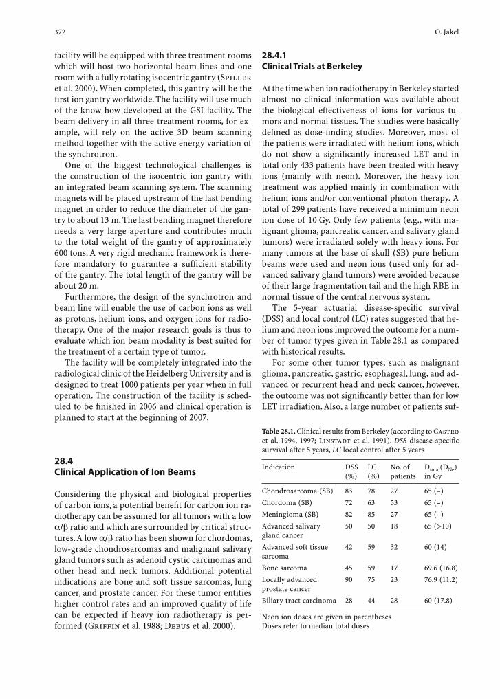
372 O. Jäkel

facility will be equipped with three treatment rooms which will host two horizontal beam lines and one room with a fully rotating isocentric gantry (Spiller et al. 2000). When completed, this gantry will be the fi rst ion gantry worldwide. The facility will use much of the know-how developed at the GSI facility. The beam delivery in all three treatment rooms, for ex-ample, will rely on the active 3D beam scanning method together with the active energy variation of the synchrotron.

One of the biggest technological challenges is the construction of the isocentric ion gantry with an integrated beam scanning system. The scanning magnets will be placed upstream of the last bending magnet in order to reduce the diameter of the gan-try to about 13 m. The last bending magnet therefore needs a very large aperture and contributes much to the total weight of the gantry of approximately 600 tons. A very rigid mechanic framework is there-fore mandatory to guarantee a suffi cient stability of the gantry. The total length of the gantry will be about 20 m.

Furthermore, the design of the synchrotron and beam line will enable the use of carbon ions as well as protons, helium ions, and oxygen ions for radio-therapy. One of the major research goals is thus to evaluate which ion beam modality is best suited for the treatment of a certain type of tumor.

The facility will be completely integrated into the radiological clinic of the Heidelberg University and is designed to treat 1000 patients per year when in full operation. The construction of the facility is sched-uled to be fi nished in 2006 and clinical operation is planned to start at the beginning of 2007.

28.4 Clinical Application of Ion Beams

Considering the physical and biological properties of carbon ions, a potential benefi t for carbon ion ra-diotherapy can be assumed for all tumors with a low

/ ratio and which are surrounded by critical struc-tures. A low / ratio has been shown for chordomas, low-grade chondrosarcomas and malignant salivary gland tumors such as adenoid cystic carcinomas and other head and neck tumors. Additional potential indications are bone and soft tissue sarcomas, lung cancer, and prostate cancer. For these tumor entities higher control rates and an improved quality of life can be expected if heavy ion radiotherapy is per-formed (Griffi n et al. 1988; Debus et al. 2000).

28.4.1 Clinical Trials at Berkeley

At the time when ion radiotherapy in Berkeley started almost no clinical information was available about the biological effectiveness of ions for various tu-mors and normal tissues. The studies were basically defi ned as dose-fi nding studies. Moreover, most of the patients were irradiated with helium ions, which do not show a signifi cantly increased LET and in total only 433 patients have been treated with heavy ions (mainly with neon). Moreover, the heavy ion treatment was applied mainly in combination with helium ions and/or conventional photon therapy. A total of 299 patients have received a minimum neon ion dose of 10 Gy. Only few patients (e.g., with ma-lignant glioma, pancreatic cancer, and salivary gland tumors) were irradiated solely with heavy ions. For many tumors at the base of skull (SB) pure helium beams were used and neon ions (used only for ad-vanced salivary gland tumors) were avoided because of their large fragmentation tail and the high RBE in normal tissue of the central nervous system.

The 5-year actuarial disease-specifi c survival (DSS) and local control (LC) rates suggested that he-lium and neon ions improved the outcome for a num-ber of tumor types given in Table 28.1 as compared with historical results.

For some other tumor types, such as malignant glioma, pancreatic, gastric, esophageal, lung, and ad-vanced or recurrent head and neck cancer, however, the outcome was not signifi cantly better than for low LET irradiation. Also, a large number of patients suf-

Table 28.1. Clinical results from Berkeley (according to Castro et al. 1994, 1997; Linstadt et al. 1991). DSS disease-specifi c survival after 5 years, LC local control after 5 years

Indication DSS(%)

LC(%)

No. of patients

Dtotal(DNe) in Gy

Chondrosarcoma (SB) 83 78 27 65 (–)

Chordoma (SB) 72 63 53 65 (–)

Meningioma (SB) 82 85 27 65 (–)

Advanced salivary gland cancer

50 50 18 65 (>10)

Advanced soft tissue sarcoma

42 59 32 60 (14)

Bone sarcoma 45 59 17 69.6 (16.8)

Locally advanced prostate cancer

90 75 23 76.9 (11.2)

Biliary tract carcinoma 28 44 28 60 (17.8)

Neon ion doses are given in parenthesesDoses refer to median total doses

Heavy Ion Radiotherapy 373

fered from severe radiation-induced toxicity, which was attributed to the high LET of neon ions and the drawbacks of the passive beam delivery system. A signifi cant improvement in outcome was, however, observed for patients treated between 1987 and 1992, which is attributed to improvements in 3D treatment planning, patient immobilization, and availability of MRI. A review of the clinical data is given by Castro (1997), Castro et al. (1994), and Linstadt et al. (1991).

28.4.2 Clinical Trials and Routine Treatments at GSI

Since December 1997, more than 220 patients have been treated with carbon ion radiotherapy at GSI. An overview over the results is given by Schulz-Ertner et al. (2003a). Patients with chordomas (n=44) and low-grade chondrosarcomas (n=23) of the skull base were treated within a clinical phase-I/II trial with carbon ion radiotherapy only. Median dose was 60 Gy (20 fractions, each 3 Gy). In February 2003 the me-dian follow-up was 20 months. Actuarial 3-year lo-

cal control rate was 100% for chondrosarcomas and 81% for chordomas of the skull base, respectively. Actuarial 3-year overall survival was 91%. Toxicity correlated with radiobiological model estimations. Late toxicity greater than common toxicity criteria (CTC) grade 3 was not observed (Schulz-Ertner et al. 2003a). Local control rates after carbon ion radiotherapy are at least comparable to the results after proton radiotherapy (Noel et al. 2001), which is currently considered the treatment of choice in chordomas and low-grade chondrosarcomas; there-fore, carbon ion radiotherapy is offered at GSI as a routine treatment to patients suffering from these tumors as an alternative to proton radiotherapy since January 2002.

Figure 28.5 shows an example of a treatment plan for patient with a chondrosarcoma close to the brain stem. The excellent dose conformation of the 90% iso-dose to the target is clearly demonstrated, although only two horizontal treatment fi elds were used here. The dose sparing of the relevant organs at risk can be seen in the dose volume histogram (Fig. 28.5b).

A clinical phase-I/II study of combined photon radiotherapy plus a carbon ion boost for sacral/spi-

Fig. 28.5a,b. Example of a treatment plan for fully fraction-ated radiotherapy using two nearly opposing fi elds of carbon ions, as it was performed at GSI. In a the dose distribution at isodose levels of 10, 30, 50, 70, and 90%V is shown, respectively. The 100% dose corresponds to 60 Gy, which was applied in 20 consecutive fractions of 3 Gy. In b the dose volume histogram for the target and these organs at risk are shown

b

a

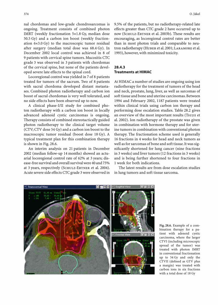
374 O. Jäkel

nal chordomas and low-grade chondrosarcomas is ongoing. Treatment consists of combined photon IMRT (weekly fractionation 5×1.8 Gy, median dose 50.5 Gy) and a carbon ion boost (weekly fraction-ation 6×3.0 Gy) to the macroscopic tumor residual after surgery (median total dose was 68.4 Gy). In December 2002 local control was achieved in 8 of 9 patients with cervical spine tumors. Mucositis CTC grade 3 was observed in 3 patients with chordomas of the cervical spine, but none of the patients devel-oped severe late effects to the spinal cord.

Locoregional control was yielded in 7 of 8 patients treated for tumors of the sacrum. Two of 8 patients with sacral chordoma developed distant metasta-ses. Combined photon radiotherapy and carbon ion boost of sacral chordomas is very well tolerated, and no side effects have been observed up to now.

A clinical phase-I/II study for combined pho-ton radiotherapy with a carbon ion boost in locally advanced adenoid cystic carcinomas is ongoing. Therapy consists of combined stereotactically guided photon radiotherapy to the clinical target volume (CTV; CTV dose 54 Gy) and a carbon ion boost to the macroscopic tumor residual (boost dose 18 Gy). A typical treatment plan for this combination therapy is shown in Fig. 28.6.

An interim analysis on 21 patients in December 2002 (median follow-up 14 months) showed an actu-arial locoregional control rate of 62% at 3 years; dis-ease-free survival and overall survival were 40 and 75% at 3 years, respectively (Schulz-Ertner et al. 2004). Acute severe side effects CTC grade 3 were observed in

9.5% of the patients, but no radiotherapy-related late effects greater than CTC grade 2 have occurred up to now (Schulz-Ertner et al. 2003b). These results are encouraging, as locoregional control rates are better than in most photon trials and comparable to neu-tron radiotherapy (Huber et al. 2001; Laramore et al. 1993), however, with minimized toxicity.

28.4.3 Treatments at HIMAC

At HIMAC a number of studies are ongoing using ion radiotherapy for the treatment of tumors of the head and neck, prostate, lung, liver, as well as sarcomas of soft tissue and bone and uterine carcinomas. Between 1994 and February 2002, 1187 patients were treated within clinical trials using carbon ion therapy and performing dose escalation studies. Table 28.2 gives an overview of the most important results (Tsujii et al. 2002). Ion radiotherapy of the prostate was given in combination with hormone therapy and for uter-ine tumors in combination with conventional photon therapy. The fractionation scheme used is generally 16 fractions in 4 weeks for head and neck tumors as well as for sarcomas of bone and soft tissue. It was sig-nifi cantly shortened for lung cancer (nine fractions in 3 weeks) and liver tumors (12 fractions in 3 weeks) and is being further shortened to four fractions in 1 week for both indications.

The latest results are from dose escalation studies in lung tumors and soft tissue sarcoma.

Fig. 28.6. Example of a com-bination therapy for a pa-tient with adenoid cystic carcinoma, where the larger CTVI (including microscopic spread of the tumor) was treated with photon IMRT in conventional fractionation up to 54 Gy and only the CTVII (defi ned as GTV plus a margin) was treated with carbon ions in six fractions with a total dose of 18 Gy

Heavy Ion Radiotherapy 375

In two phase-I/II trials for stage-I non-small cell lung cancer (NSCLC), using different fractionation schemes (18 fractions in 6 weeks and 9 fractions in 3 weeks), a dose escalation was performed from 59.4 to 94.5 Gy and from 68.4 to 79.2 Gy, respectively (Miyamoto et al. 2003; Koto et al. 2004). The result-ing overall control rates for the 6- and 3-week frac-tionation were 64 and 84%, respectively. The total recurrence rate was 23.2%.

For unresectable bone and soft tissue sarcomas, a further phase-I/II trial was performed with doses be-tween 52.8 and 73.6 Gy (Kamada et al. 2002), applied in 16 fractions over 4 weeks. The observed overall control rates were 88 and 73% at 1 year and 3 years, respectively.

28.5 Outlook

In the past decade, valuable clinical experience has been gained in heavy ion therapy at HIMAC and GSI. Together with the development of new technologies, especially for beam application and treatment plan-ning, there will certainly be a broader implementation of ions in clinical settings that allow for an optimal exploitation of the physical and biological potential of protons and heavy ions. Among these technologies are inverse treatment planning for particles (Oelfke and Bortfeld 2000, 2001), gating for breath-depen-dent targets (Minohara et al. 2000; Shirato et al. 2000; Ford et al. 2002), the raster scan system for tumor conform beam application (Haberer et al. 1993), and biological plan optimization for carbon ion radiotherapy (Scholz et al. 1997; Krämer and Scholz 2000; Krämer et al. 2000).

Further research is still required to clarify what indications benefi t most from heavy ion therapy and what is the ideal ion species and fractionation scheme. These questions can be answered only in

clinical studies performed at dedicated ion facili-ties such as the HIMAC, HIBMC, or the upcoming Heidelberg facility.

For tumors with proven effectiveness of carbon ion radiotherapy, such as chordomas and low-grade chondrosarcomas of the skull base, clinical phase-III trials are necessary to determine the advantages of carbon ion radiotherapy over other radiotherapy modalities such as modern photon techniques (like IMRT) or proton radiotherapy which is currently considered to be the treatment of choice. Toxicity, quality of life, and socio-economic aspects have to be investigated as study end points besides local control probability.

The encouraging results from HIMAC, especially for bone and soft tissue sarcomas as well as for lung tumors, warrant further clinical investigation of car-bon ion radiotherapy in the treatment of these tu-mors. Clinical phase-III studies will have to be con-ducted and will not only have to compare different radiotherapy modalities but will have to include a control arm of surgically treated patients.

New immobilization techniques with rigid im-mobilization devices and pre-treatment control and correction of the patient alignment, together with the development of faster dose calculation and optimi-zation algorithms and better knowledge of the com-plex biology of carbon ions, will help to enlarge the spectrum of possible indications for carbon ion ra-diotherapy. The development of a gantry for carbon ion radiotherapy will facilitate the safe treatment of paraspinal tumors by allowing posterior beam direc-tions.

Further investigation is needed in the fi eld of mul-timodality treatments. There is almost no clinical data available about adjuvant chemotherapy or hormone therapy, although interdisciplinary treatment of pa-tients with tumors that tend to metastasize seems to be warranted. In this connection, major attention has to be drawn to the proper defi nition of clinical trials for head and neck malignancies, gynecological tu-

Table 28.2. Results from HIMAC (Tsujii et al. 2002). Local control (LC) and overall survival (OS) are given for 2 and 3 years and refers to the latest completed trial (patient numbers in parentheses).

Indication LC (2 years; %) OS (3 years; %) Patients D(C12) in Gy

Locally advanced head and neck tumors 61 42 170 (134) 52.8–64

Lung cancer (stage I) 100 73 161 (50) 72

Hepatocellular carcinoma (stage T2-4N0M0) 83 45 122 (86) 49.5–79.5

Prostate carcinoma (stage T1-3N0M0) 100 97 143 (61) 60–66

Squamous cell carcinoma (uterus; stage T2-4N0M0) 67 36 67 (14) 68.8–72.8

Unresectable bone and soft tissue sarcoma 77 50 95 (64) 52.8–73.6

376 O. Jäkel

mors, and prostate cancer in order to obtain compa-rability with up-to-date oncological standard therapy regimes.

A combination of different radiotherapy modali-ties, such as photon IMRT plus carbon ions or pro-tons, might be favorable for a number of indications. Combined radiotherapy offers the possibility for risk-adapted treatment of different target volumes in one patient dependent on the oncological concept based on risk estimation. Furthermore, the combina-tion of carbon ion radiotherapy or protons with pho-ton radiotherapy will guarantee that a higher number of patients will benefi t from the advantages of par-ticle radiotherapy despite the still limited availability. Possible indications are head and neck malignancies, malignant primary brain tumors, and prostate can-cer. For patients with unfavorable localized prostate cancer a clinical phase-I/II trial of combined photon IMRT with a carbon ion boost, which is a project of the European hadrontherapy network “ENLIGHT,” is in preparation (Nikoghosyan et al. 2004).

Due to the biological properties of carbon ion radiotherapy, hypofractionation might be consid-ered for a number of tumor entities. The accelerated fractionation scheme used at GSI for chordomas and low-grade chondrosarcomas of the skull base corre-sponds to a reduction of treatment time by about 50% compared with conventional photon radiotherapy. First clinical hypofractionation trials for lung cancer are underway at HIMAC and further studies are in preparation. These studies investigate outcome and toxicity of hypofractionation as end points, as well as quality of life and economic aspects. Carbon ion radiotherapy might even turn out to be an optimal treatment option from an economic point of view, as hypofractionation leads to substantial reduction of overall treatment time and hospitalization.

References

Bendl R, Pross J, Schlegel W (1993) VIRTUOS: a program for VIRTUal radiotherapy simulation. In: Lemke HU, Inamura K, Jaffe CC, Felix R (eds) Computer assisted radiology. Proc Int Symp CAR 93. Springer, Berlin Heidelberg New York, pp 676–682

Castro JR (1997) Clinical programs: a review of past and exist-ing hadron protocols. In: Amaldi U, Larrson B, Lemoigne Y (eds) Advances in hadrontherapy. Elsevier, Amsterdam, pp 79–94

Castro J, Lawrence J (1978) Heavy ion radiotherapy. In: Law-rence JH, Budinger TF(eds) Recent advances in nuclear medicine, Grune & Stratton vol 5. New York, pp 119–137

Castro JR, Linstadt DE, Bahary J-P et al. (1994) Experience in charged particle irradiation of tumors of the skull base 1977–1992. Int J Radiat Oncol Biol Phys 29:647–655

Chen G, Singh R, Castro J, Lyman J, Quivey J (1979) Treatment planning for heavy ion radiotherapy. Int J Radiat Oncol Biol Phys 5:1809–1819

Debus J, Haberer T, Schulz-Ertner D et al. (2000) Fractionated carbon ion irradiation of skull base tumours at GSI. First clinical results and future perspectives. Strahlenther Onkol 176:211–216

Eickhoff H, Böhne D, Debus J, Haberer T, Kraft G, Pavlovich M (1998) The proposed accelerator for light ion cancer therapy in Heidelberg. GSI Scientifi c Report, Darmstadt, Germany, pp 164–165

Eickhoff H, Haberer T, Kraft G, Krause U, Richter M, Steiner R, Debus J (1999) The GSI cancer therapy project. Strahlen-ther Onkol 175 (Suppl 2):21–24

Endo M, Koyama-Ito H, Minohara S, Miyahara N, Tomura H, Kanai T, Kawachi K, Tsujii H, Morita K (1996) HIPLAN: a heavy ion treatment planning system at HIMAC. J Jpn Soc Ther Radiol Oncol 8:231–238

Ford EC, Mageras GS, Yorke E, Rosenzweig KE, Wagman R, Ling CC (2002) Evaluation of respiratory movement during gated radiotherapy using fi lm and electronic portal imag-ing. Int J Radiat Oncol Biol 52:522–531

Goldstein LS, Phillips TL, Ross GY (1981) Biological effects of accelerated heavy ions. II. Fractionated irradiation of intes-tinal crypt cells. Radiat Res 86:542–558

Griffi n TW, Wambersie A, Laramore G, Castro J (1988) Interna-tional clinical trials in radiation oncology. High LET: heavy particle trials. Int J Radiat Oncol Biol Phys 14 (Suppl 1):S83–S92

Haberer T, Becher W, Schardt D, Kraft G (1993) Magnetic scanning system for heavy ion therapy. Nucl Instrum Meth A330:296–305

Heeg P, Eickhoff H, Haberer T (2004) Die Konzeption der Heidelberger Ionentherapieanlage HICAT. Z Med Phys 14:17–24

Huber PE, Debus J, Latz D et al. (2001) Radiotherapy for advanced adenoid cystic carcinoma: neutrons, photons or mixed beam? Radiother Oncol 59:161–167

Itano A, Akagi T, Higashi A et al. (2003) Operation of medi-cal accelerator PATRO at Hyogo Ion Beam Medical Center. Workshop on Accelerator Operation, 10–14 March, Tsu-kuba, Japan

Jäkel O, Jacob C, Schardt D, Karger CP, Hartmann GH (2001a) Relation between carbon ions ranges and X-ray CT num-bers. Med Phys 28:701–703

Jäkel O, Krämer M, Karger CP, Debus J (2001b) Treatment plan-ning for heavy ion radio-therapy: clinical implementation and application. Phys Med Biol 46:1101–1116

Jäkel O, Schulz-Ertner D, Karger CP, Nikoghosyan A, Debus J (2003) Heavy ion therapy: status and perspectives. Technol Cancer Res Treat 2:377–388

Kamada T, Tsujii H, Mizoe J et al. (1999) A horizontal CT system dedicated to heavy-ion beam treatment. Radiother Oncol 50:235–237

Kamada T, Tsujii H, Tsuji H et al. (2002) Effi cacy and safety of carbon ion radiotherapy in bone and soft tissue sarcomas. J Clin Oncol 20:4466–4471

Kanai T, Endo M, Minohara S et al. (1999) Biophysical charac-teristics of HIMAC clinical irradiation system for heavy-ion radiation therapy. Int J Radiat Oncol Biol Phys 44:201–210

Heavy Ion Radiotherapy 377

Koto M, Miyamoto T, Yamamoto N, Nishimura H, Yamada S, Tsujii H (2004) Local control and recurrence of stage I non-small cell lung cancer after carbon ion radiotherapy. Radiother Oncol 71:147–156

Krämer M, Scholz M (2000) Treatment planning for heavy ion radiotherapy: calculation and optimization of biologically effective dose. Phys Med Biol 45:3319–3330

Krämer M, Jäkel O, Haberer T, Kraft G, Schardt D, Weber U (2000) Treatment planning for heavy ion radiotherapy: physical beam model and dose optimization. Phys Med Biol 45:3299–3317

Laramore GE, Krall JM, Thomas FJ et al. (1993) Fast neutron radiation therapy for locally advanced prostate cancer: fi nal report of an RTOG randomized clinical trial. Am J Clin Oncol 16:164

Linstadt DE, Castro JR, Phillips TL (1991) Neon ion radiother-apy: results of the phase I/II clinical trial. J Radiat Oncol Biol Phys 20:761–769

Minohara S, Kanai T, Endo M, Kawachi K (1993) Effects of object size on a function to convert X-Ray CT numbers into the water equivalent path length of charged particle beam. In: Ando K, Kanai T(eds) Proc Third Workshop on Physical and Biological Research with Heavy Ions, Chiba, Japan, pp 14–15

Minohara S, Kanai T, Endo M, Noda K, Kanazawa M (2000) Respiratory gated irradiation system for heavy-ion radio-therapy. Int J Radiat Oncol Biol Phys 47:1097–1103

Miyamoto T, Yamamoto N, Nishimura H et al. (2003) Carbon ion radiotherapy for stage I non-small cell lung cancer. Radiother Oncol 66:127–140

Nikoghosyan A, Schulz-Ertner D, Didinger B, Jäkel O, Zuna I, Höss A, Wannenmacher M, Debus J (2004) Evaluation of therapeutic potential of heavy ion therapy for patients with locally advanced prostate cancer. Int J Radiat Oncol Biol Phys 58:89–97

Noel G, Habrand JL, Mammar H et al. (2001) Combination of

photon and proton radiation therapy for chordomas and chondrosarcomas of the skull base: the Centre de Proton-therapie d’Orsay experience. Int J Radiat Oncol Biol Phys 51:392–398

Oelfke U, Bortfeld T (2000) Intensity modulated radiotherapy with charged particle beams: studies of inverse treatment planning for rotation therapy. Med Phys 27:1246–1257

Oelfke U, Bortfeld T (2001) Inverse planning for photon and proton beams. Med Dosim 26:113–124

Scholz M, Kellerer AM, Kraft-Weyrather W, Kraft G (1997) Computation of cell survival in heavy ion beams for ther-apy: the model and its approximation. Radiat Environ Bio-phys 36:59–66

Schulz-Ertner D, Nikoghosyan A, Jäkel O et al. (2003b) Feasi-bility and toxicity photon and carbon ion radiotherapy for locally advanced adenoid cystic carcinomas. Int. J. Radiat. Oncol. Biol. Phys. 56(2):391–398

Shirato H, Shimizu S, Kunieda T, Kitamura K, van Herk M, Kagei K, Nishioka T, Hashimoto S, Fujita K, Aoyama H, Tsuchiya K, Kudo K, Muyasaka K (2000) Physical aspects of a real-time tumor-tracking system for gated radiotherapy. Int J Radiat Oncol Biol Phys 48:1187–1195

Sisterson J (ed) (2003) Particle newsletter 31, Harvard, Boston, Massachusetts

Spiller P, Boehne D, Dolinskii A et al. (2000) Gantry studies for the proposed heavy ion cancer therapy facility in Heidel-berg. Proc 7th European Particle Accelerator Conference (EPAC). Cern, Geneva, pp 2551–2553

Tepper J, Verhey L, Goitein M et al. (1977) In vivo determi-nations of RBE in a high energy modulated proton beam using normal tissue reactions and fractionated dose sched-ules. Int J Radiat Oncol Biol Phys 2:1115–1122

Tsujii H, Morita S, Miyamoto T et al. (2002) Experiences of carbon ion radiotherapy at NIRS. In: Kogelnik HD, Sedl-mayer F (eds) Progress in radio-oncology, vol 7. Monduzzi Editore, Bologna, pp 393–405

Permanent-Implant Brachytherapy in Prostate Cancer 379

29 Permanent-Implant Brachytherapy in Prostate Cancer

Marco Zaider

M. Zaider, PhDDepartment of Medical Physics, Memorial Sloan-Kettering Cancer Center, 1275 York Avenue, New York, NY 10021, USA

29.1 Introduction

The overall survival benefi ts of transperineal per-manent interstitial implantation among men with early, localized prostate cancer remain uncertain (Albertsen et al. 1998; Chodak 1998). In favor-able-risk patients [prognosis category is defi ned by pre-treatment prostate-specifi c antigen (PSA), Gleason score, and tumor stage] this form of treat-ment is associated with excellent biochemical (gener-ally defi ned as an undetectable PSA concentration) outcome – close to 90% PSA relapse-free survival at 5 years, a number which compares favorably with outcomes from other forms of local treatment (e.g., external-beam radiotherapy, radical prostatectomy; Peschel and Colberg 2003). This comes, however, with a price tag, namely the risk of (occasionally permanent) rectal and particularly urinary (grade-2 urinary symptoms represent the most common tox-icity after prostate brachytherapy) toxicity, as well as sexual dysfunction (Jani and Hellman 2003; Sandhu et al. 2000; Zelefsky et al. 2000a). For many patients with early, localized prostate cancer the decision to undergo a treatment of questionable

benefi t, yet tangibly impacting upon their quality of life (QOL), is understandably diffi cult. As a result, di-minishing the risk of complications, and at the same time maintaining good dosimetric coverage of the tumor, remains the overriding concern in prostate brachytherapy. (Brachytherapy may be less likely to result in impotence in urinary incontinence than other forms of treatment.)

With this in mind, we discuss herein several fac-tors that impact on the quality of the implant. These include:1. Conventional (dosimetric) treatment planning:

Much treatment planning in brachytherapy contin-ues to be performed suboptimally, i.e., by manual (trial-and-error) methods. Applied mathematics has a well-developed repertory of optimization tools (simulated annealing, genetic algorithm, integer programming) that could, and must, be implemented in treatment planning software.

2. Biological treatment planning refers to incorporat-ing in treatment planning information on tumor control probability (TCP) and normal-tissue com-plication probability (NTCP) for all structures of interest. Plan optimization would then be per-formed based on an overall fi gure of merit (FM), rather than dosimetrically, as is currently done.

3. Treatment delivery: It is often the case that the insertion of various applicators in or near the intended target results in changes in the target geometry. These changes, and their evolution in time, must be anticipated in the treatment plan – and corrected for. Of particular importance is to make the process of treatment delivery as much as possible operator independent. For instance, in permanent prostate implants there is a recognized variance between the intended radioisotope posi-tions and their actual location in the gland. Imag-ing tools capable of reconstructing in real time the positions of radioisotopes already inserted could be used to re-optimize the plan.

4. Imaging: Alongside MRI and sextant biopsy, MR spectroscopy (MRS) has been used to identify non-invasively clinically signifi cant tumor An

CONTENTS

29.1 Introduction 37929.2 Treatment Planning 38029.2.1 Outline 38029.2.2 Dose Prescription 38029.2.3 Dose Calculation Checks 38129.2.4 Treatment-Plan Optimization 38129.2.5 Example 38229.3 Functional Imaging 38329.4 Biological Optimization 38329.5 Some Unanswered Questions 386 References 386

380 M. Zaider

argument can be made, based on TCP models, that in brachytherapy one expects a clinical advan-tage when the (inevitable) dosimetric hot spots are placed at MRS-positive voxels rather than at random locations in the gland.

The methodology described below refl ects, as might be expected, accepted practice at Memorial Sloan-Kettering Cancer Center (MSKCC).

29.2 Treatment Planning

29.2.1 Outline

Pre-planning in prostate brachytherapy (meaning that the plan was generated several days or a week before implantation) has a number of well-recog-nized defi ciencies (Nag et al. 2001):1. It is diffi cult to duplicate the patient position in

the operating room to match the patient position during the pre-planning simulation.

2. Patient geometry can change over time, e.g., urine in the bladder or feces in the rectum may swell the prostate.

3. A pre-treatment plan may prove impossible to implement due to the needle site being blocked by the pubic symphysis.

At MSKCC the intraoperative treatment-planning sequence is as follows: The patient is placed in the ex-tended lithotomy position and a urinary catheter is in-serted. The ultrasound probe is positioned in the rec-tum and needles are inserted along the periphery of the prostate using a perineal template as a guide. Axial images of the prostate are acquired at 0.5 cm spacing (from base to apex), transferred to the treatment plan-ning system using a PC-based video capture system, and calibrated. For each ultrasound image, prostate and urethra contours as well as the anterior position of the rectal wall are entered. Needle positions are identi-fi ed on the ultrasound images and correlated with the US template locations. The contours, dose reference points, needle coordinates, and data describing the isotope/activity available along with predetermined dose constraints and their respective weights serve as input for the dose-optimization algorithm.

Dose optimization is achieved using a genetic al-gorithm (GA) as described below. Isodose distribu-tions for each axial cut and dose-volume histograms

(DVH) for the structures of interest (prostate, ure-thra, and rectum) are calculated and inspected in the operating room. The 125I or 103Pd radioisotopes are individually loaded using a Mick applicator. The en-tire planning process from the contouring of images to the generation of the radioisotope loading pattern requires approximately 10–15 min.

About 4 h after the implant, post-implantation CT scans are obtained. For dosimetric evaluation of the implant the prostate, urethra, and rectum are contoured on each axial CT image, and the param-eters recommended by the American Brachytherapy Society (Nag et al. 2001) are calculated and compared with the original plan.

29.2.2 Dose Prescription

Dose prescription in prostate brachytherapy makes use of the concept of minimum peripheral dose (mPD), which is defi ned as the largest-dose isodose surface that completely surrounds the clinical target. This approach has been endorsed by the American Brachytherapy Society (Nag et al. 2001). The mPD is very sensitive to minor variations in the planned do-simetry because it is always given by the lowest dose delivered to any volume of the target – however small. (If 99.9% of the target is covered by the prescription dose and the dose delivered to the remaining 0.1% of the volume is, for example, 10% of the prescription dose, it is this latter number that decides the value of the mPD.) This problem may be avoided by relaxing the requirement that the prescription isodose surface cover 100% of the target; instead, the so-called Dx method can be adopted, which means that a dose of at least Dx is required to be delivered to x% of the target volume. A typical value is D95 (D100 is, of course, the same as mPD).

The dose constraints for prostate implants are as follows (Zelefsky et al. 2000b): mPD to target 144 Gy for 125I and 140 Gy for 103Pd, and the urethra and the rectum are to receive no more than 120% and 78% of the prescription dose, respectively. Typically, we use radioisotopes with air kerma strength of 0.4 U (125I) and 3 U (103Pd).

Permanent-Implant Brachytherapy in Prostate Cancer 381

29.2.3 Dose Calculation Checks

It is common practice at MSKCC to have an indepen-dent review of the dose calculation. The review is per-formed in the operating room prior to radioisotope implantation by a physicist different from the one that calculated the plan. The review determines that:1. The computer software has been used appropri-

ately2. Prescription dose is correct3. User-supplied input data (e.g., isotope, source

activity) are accurate4. Output data look “reasonable”5. The number of radioisotopes calculated with

nomograms (see below) is within 10% of the number used in the plan

Nomograms for permanent volume implants are tools designed to predict the total air kerma strength, SK, necessary to deliver a stated dose to a known tar-get volume. More precisely, they stipulate the total source strength, SK, such that the isodose surface corresponding to the prescription dose has a stated volume. The volume nomograms given here (Cohen et al. 2002) were obtained in connection with perma-nent prostate implants and thus, strictly speaking, the volume in question refers to the geometry of this particular organ.

For a 125I permanent implant and a prescription dose of 144 Gy:

2.2

5.709 3

1.524 3

avgavg

k

avgavg

dd cm

cmSU d

d cmcm

⎧ ⎛ ⎞≤⎪ ⎜ ⎟

⎝ ⎠⎪= ⎨⎛ ⎞⎪ >⎜ ⎟⎪ ⎝ ⎠⎩

(1)

For a 103Pd permanent implant and a prescription dose of 140 Gy:

2.56

29.41 3

5.395 3

avgavg

k

aveavg

dd cm

cmSU d d cm

cm

⎧ ⎛ ⎞≤⎪ ⎜ ⎟

⎪ ⎝ ⎠= ⎨⎪ ⎛ ⎞ >⎜ ⎟⎪ ⎝ ⎠⎩

(2)

The quantity davg refers to the average of three or-thogonal dimensions of the volume to be implanted. In a typical application of these equations davg is evalu-ated and then the total number of radioactive sources needed is calculated by dividing the total required source strength, SK, by the single-seed strength.

29.2.4 Treatment-Plan Optimization

Potential source positions are localized with respect to a template that is placed in a fi xed position rela-tive to the treatment region (the prostate gland). The template, shown in Fig. 29.1, has a rectangular pattern of holes. Needles are inserted through the template grid and radioisotopes are placed along each needle at positions (typically in multiples of 0.5 cm) deter-mined by the treatment plan. A series of parallel ul-trasound (US) images is taken through the prostate and fi rmware in the ultrasound unit overlays a grid of dots onto these images that correspond to the tem-plate holes. The grid coordinates on the template and the distance of the US image away from the template uniquely identify the 3D coordinates of each potential radioisotope position relative to the gland anatomy. If inserted needles deviate from the initial grid coordi-nates, the planning system has provisions for taking this into account in dosimetric calculations.

In the treatment-planning code used at MSKCC optimized radioisotope locations are determined us-ing a genetic algorithm engine (Silvern 1998; Lee et al. 1999). The GA is a formalism that imitates the principle of “natural selection” (Chambers 1995; Grefenstette et al. 1987; Man et al. 1999; Zalzala and Fleming 1997). A “chromosome” is defi ned as a sequence of binary data, e.g., for prostate brachyther-apy each chromosome represents a specifi c radioiso-tope-loading pattern. A collection of chromosomes is referred to as a “population.” A symbol in a chro-mosome represents a location where a source can be placed in the prostate. A 0/1 bit indicates the absence (or presence) of a radioactive seed at that particular location. Using this encoding scheme, each chromo-

Fig. 29.1. Template used in a prostate-permanent implant

382 M. Zaider

some completely defi nes an individual treatment plan. Every chromosome in the population is evalu-ated by an objective function, which calculates the doses to all of the recorded optimization points and evaluates how many of these points fall within speci-fi ed dose tolerances. The larger the number of points, the higher the score the chromosome receives.

For instance (Silvern 1998), let PD be the pre-scription dose; the prostate score is the number of (uniformity) points that satisfy PD D 1.6PD, the urethral score is the number of points in the urethra for which D 1.2PD, and the rectal score sums up all points in the rectum for which D 0.78PD. From this, a raw score is obtained:

Raw score = 5* (prostate score) + 35* (rectal score) + 50* (urethral score) (3)

and a fi nal score (used in the optimization algorithm) which is a linear function of the raw score [=A*(raw score)+B].

Higher-scoring chromosomes are selectively fa-vored to act as parent chromosomes to produce the next generation. Lower-scoring chromosomes, how-ever, still have a chance of being selected to act as par-ents. This helps keep the population diversifi ed. The parameters of the objective function include a set of predetermined dose constraints and their respective relative weight factors (e.g., 0.2 for the prostate, 10 for the urethra, 7 for the rectum). Formally, the following steps are followed:1. Selected parent chromosomes are paired off and

sections of these parent chromosomes are inter-changed to yield two new “baby” chromosomes (this mimics biological crossover).

2. The newly formed progeny chromosomes are mutated. Mutation is performed by randomly inverting several bits (a 1 is changed to a 0, and vice versa). The mutation probability of each symbol is of the order of 1%. This mutation prob-ability was found to keep the population diversi-fi ed while not excessively destroying high-quality bit combinations.

3. Next, the chromosomes are again evaluated by the objective function. A new set of parent chromo-somes is selected from the population favoring higher-scoring individuals and a new “pass” is started.

The process is repeated for a suffi cient number of generations (typically 6000) to repeatedly and reli-ably yield an adequate treatment plan in a reasonable amount of time.

Other optimization algorithms used in prostate brachytherapy are simulated annealing (Sloboda 1992; Pouliot et al. 1996) and branch-and-bound (Gallagher and Lee 1997; Lee et al. 1999; Zaider et al. 2000).

29.2.5 Example

Figure 29.2 shows a typical 2D ultrasound image with prostate and urethra contours and needle positions. Also shown are isodose contours and seed positions as determined by the GA code. The determination that the treatment plan achieves the required mPD or D90 can be made with the aid of dose-volume histograms (DVH), which plot as a function of dose,

Fig. 29.2. Dose prescription for a permanent prostate implant. In this ultrasound image the white line delineates the prostate and the 100% isodose line (mPD=144 Gy) is shown in green. Green dots indicate seeds and red dots show unused seed locations along needles

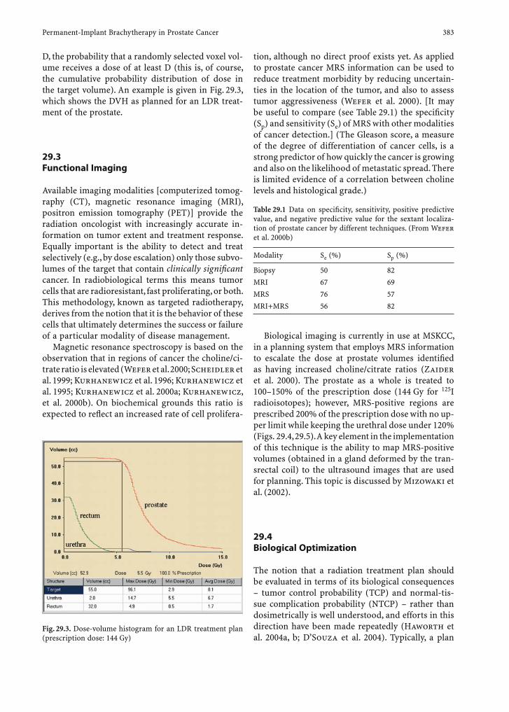
Permanent-Implant Brachytherapy in Prostate Cancer 383

D, the probability that a randomly selected voxel vol-ume receives a dose of at least D (this is, of course, the cumulative probability distribution of dose in the target volume). An example is given in Fig. 29.3, which shows the DVH as planned for an LDR treat-ment of the prostate.

29.3 Functional Imaging

Available imaging modalities [computerized tomog-raphy (CT), magnetic resonance imaging (MRI), positron emission tomography (PET)] provide the radiation oncologist with increasingly accurate in-formation on tumor extent and treatment response. Equally important is the ability to detect and treat selectively (e.g., by dose escalation) only those subvo-lumes of the target that contain clinically signifi cant cancer. In radiobiological terms this means tumor cells that are radioresistant, fast proliferating, or both. This methodology, known as targeted radiotherapy, derives from the notion that it is the behavior of these cells that ultimately determines the success or failure of a particular modality of disease management.

Magnetic resonance spectroscopy is based on the observation that in regions of cancer the choline/ci-trate ratio is elevated (Wefer et al. 2000; Scheidler et al. 1999; Kurhanewicz et al. 1996; Kurhanewicz et al. 1995; Kurhanewicz et al. 2000a; Kurhanewicz, et al. 2000b). On biochemical grounds this ratio is expected to refl ect an increased rate of cell prolifera-

tion, although no direct proof exists yet. As applied to prostate cancer MRS information can be used to reduce treatment morbidity by reducing uncertain-ties in the location of the tumor, and also to assess tumor aggressiveness (Wefer et al. 2000). [It may be useful to compare (see Table 29.1) the specifi city (Sp) and sensitivity (Se) of MRS with other modalities of cancer detection.] (The Gleason score, a measure of the degree of differentiation of cancer cells, is a strong predictor of how quickly the cancer is growing and also on the likelihood of metastatic spread. There is limited evidence of a correlation between choline levels and histological grade.)

Table 29.1 Data on specifi city, sensitivity, positive predictive value, and negative predictive value for the sextant localiza-tion of prostate cancer by different techniques. (From Wefer et al. 2000b)

Modality Se (%) Sp (%)

Biopsy 50 82

MRI 67 69

MRS 76 57

MRI+MRS 56 82

Biological imaging is currently in use at MSKCC, in a planning system that employs MRS information to escalate the dose at prostate volumes identifi ed as having increased choline/citrate ratios (Zaider et al. 2000). The prostate as a whole is treated to 100–150% of the prescription dose (144 Gy for 125I radioisotopes); however, MRS-positive regions are prescribed 200% of the prescription dose with no up-per limit while keeping the urethral dose under 120% (Figs. 29.4, 29.5). A key element in the implementation of this technique is the ability to map MRS-positive volumes (obtained in a gland deformed by the tran-srectal coil) to the ultrasound images that are used for planning. This topic is discussed by Mizowaki et al. (2002).

29.4 Biological Optimization

The notion that a radiation treatment plan should be evaluated in terms of its biological consequences – tumor control probability (TCP) and normal-tis-sue complication probability (NTCP) – rather than dosimetrically is well understood, and efforts in this direction have been made repeatedly (Haworth et al. 2004a, b; D’Souza et al. 2004). Typically, a plan

Fig. 29.3. Dose-volume histogram for an LDR treatment plan (prescription dose: 144 Gy)

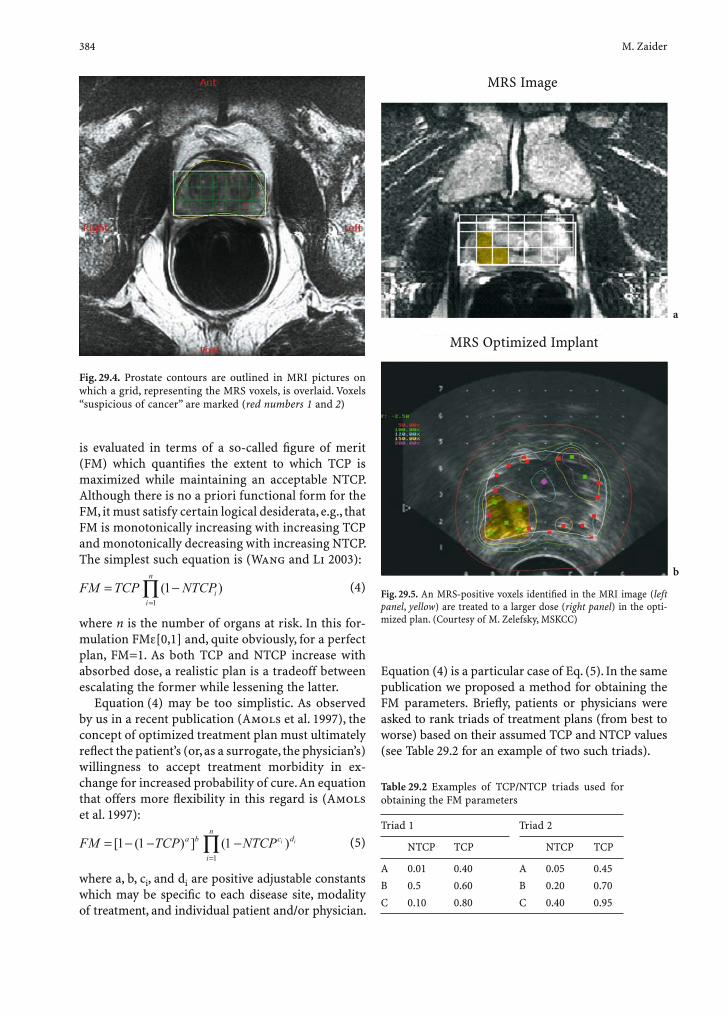
384 M. Zaider

Equation (4) is a particular case of Eq. (5). In the same publication we proposed a method for obtaining the FM parameters. Briefl y, patients or physicians were asked to rank triads of treatment plans (from best to worse) based on their assumed TCP and NTCP values (see Table 29.2 for an example of two such triads).

Table 29.2 Examples of TCP/NTCP triads used for obtaining the FM parameters

Triad 1 Triad 2

NTCP TCP NTCP TCP

A 0.01 0.40 A 0.05 0.45

B 0.5 0.60 B 0.20 0.70

C 0.10 0.80 C 0.40 0.95

b

Fig. 29.4. Prostate contours are outlined in MRI pictures on which a grid, representing the MRS voxels, is overlaid. Voxels “suspicious of cancer” are marked (red numbers 1 and 2)

Fig. 29.5. An MRS-positive voxels identifi ed in the MRI image (left panel, yellow) are treated to a larger dose (right panel) in the opti-mized plan. (Courtesy of M. Zelefsky, MSKCC)

a

is evaluated in terms of a so-called fi gure of merit (FM) which quantifi es the extent to which TCP is maximized while maintaining an acceptable NTCP. Although there is no a priori functional form for the FM, it must satisfy certain logical desiderata, e.g., that FM is monotonically increasing with increasing TCP and monotonically decreasing with increasing NTCP. The simplest such equation is (Wang and Li 2003):

1

(1 )n

ii

FM TCP NTCP=

= −∏ (4)

where n is the number of organs at risk. In this for-mulation FM [0,1] and, quite obviously, for a perfect plan, FM=1. As both TCP and NTCP increase with absorbed dose, a realistic plan is a tradeoff between escalating the former while lessening the latter.

Equation (4) may be too simplistic. As observed by us in a recent publication (Amols et al. 1997), the concept of optimized treatment plan must ultimately refl ect the patient’s (or, as a surrogate, the physician’s) willingness to accept treatment morbidity in ex-change for increased probability of cure. An equation that offers more fl exibility in this regard is (Amols et al. 1997):

[1 (1 ) ] (1 )= − − −1

i i

nc da b

i

FM TCP NTCP=∏ (5)

where a, b, ci, and di are positive adjustable constants which may be specifi c to each disease site, modality of treatment, and individual patient and/or physician.

MRS Image

MRS Optimized Implant

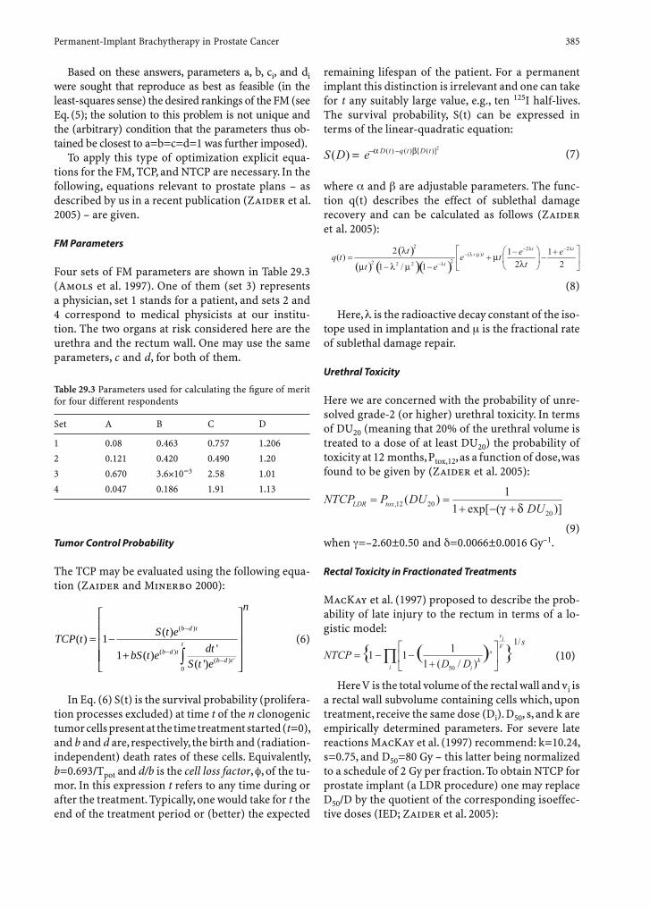
Permanent-Implant Brachytherapy in Prostate Cancer 385

Based on these answers, parameters a, b, ci, and di were sought that reproduce as best as feasible (in the least-squares sense) the desired rankings of the FM (see Eq. (5); the solution to this problem is not unique and the (arbitrary) condition that the parameters thus ob-tained be closest to a=b=c=d=1 was further imposed).

To apply this type of optimization explicit equa-tions for the FM, TCP, and NTCP are necessary. In the following, equations relevant to prostate plans – as described by us in a recent publication (Zaider et al. 2005) – are given.

FM Parameters

Four sets of FM parameters are shown in Table 29.3 (Amols et al. 1997). One of them (set 3) represents a physician, set 1 stands for a patient, and sets 2 and 4 correspond to medical physicists at our institu-tion. The two organs at risk considered here are the urethra and the rectum wall. One may use the same parameters, c and d, for both of them.

Table 29.3 Parameters used for calculating the fi gure of merit for four different respondents

Set A B C D

1 0.08 0.463 0.757 1.206

2 0.121 0.420 0.490 1.20

3 0.670 3.6×10–3 2.58 1.01

4 0.047 0.186 1.91 1.13

Tumor Control Probability

The TCP may be evaluated using the following equa-tion (Zaider and Minerbo 2000):

TCP tS t e

bS t edt

S t e

b d t

b d tb d t

t( ) ( )

( ) '( ')

( )

( )( ) '

= −+

⎡

⎣

⎢⎢⎢

−

−−∫

11

0⎢⎢

⎤

⎦

⎥⎥⎥⎥

n

(6)

In Eq. (6) S(t) is the survival probability (prolifera-tion processes excluded) at time t of the n clonogenic tumor cells present at the time treatment started (t=0), and b and d are, respectively, the birth and (radiation-independent) death rates of these cells. Equivalently, b=0.693/Tpot and d/b is the cell loss factor, , of the tu-mor. In this expression t refers to any time during or after the treatment. Typically, one would take for t the end of the treatment period or (better) the expected

remaining lifespan of the patient. For a permanent implant this distinction is irrelevant and one can take for t any suitably large value, e.g., ten 125I half-lives. The survival probability, S(t) can be expressed in terms of the linear-quadratic equation:

(7)

where and are adjustable parameters. The func-tion q(t) describes the effect of sublethal damage recovery and can be calculated as follows (Zaider et al. 2005):

( )( ) ( )( )

2 2 2( )

22 2 2

2 1 1( )2 21 / 1

t tt

t

t e eq t e ttt e

λ λλ µ

λ

λµ

λµ λ µ

− −− +

−

⎡ ⎤⎛ ⎞− += + −⎢ ⎥⎜ ⎟

⎝ ⎠− − ⎣ ⎦

(8)

Here, is the radioactive decay constant of the iso-tope used in implantation and is the fractional rate of sublethal damage repair.

Urethral Toxicity

Here we are concerned with the probability of unre-solved grade-2 (or higher) urethral toxicity. In terms of DU20 (meaning that 20% of the urethral volume is treated to a dose of at least DU20) the probability of toxicity at 12 months, Ptox,12, as a function of dose, was found to be given by (Zaider et al. 2005):

,12 2020

1( )1 exp[ ( )]LDR toxNTCP P DU

DUγ δ= =

+ − +

(9)when =–2.60±0.50 and =0.0066±0.0016 Gy–1.

Rectal Toxicity in Fractionated Treatments

MacKay et al. (1997) proposed to describe the prob-ability of late injury to the rectum in terms of a lo-gistic model:

50

1/11 11 ( / )

{ ( ) }viV

sk

i i

sNTCP

D D⎡ ⎤

= − −⎢ ⎥+⎣ ⎦∏ (10)

Here V is the total volume of the rectal wall and vi is a rectal wall subvolume containing cells which, upon treatment, receive the same dose (Di). D50, s, and k are empirically determined parameters. For severe late reactions MacKay et al. (1997) recommend: k=10.24, s=0.75, and D50=80 Gy – this latter being normalized to a schedule of 2 Gy per fraction. To obtain NTCP for prostate implant (a LDR procedure) one may replace D50/D by the quotient of the corresponding isoeffec-tive doses (IED; Zaider et al. 2005):

386 M. Zaider

( )

( )( ) '

0

1 ( )log'1 ( )

( ')

b d t

tb d t

b d t

S t eIEDdtbS t e

S t eα

−

−−

⎡ ⎤⎢ ⎥⎢ ⎥= −⎢ ⎥+⎢ ⎥

⎣ ⎦∫

(11)

In the absence of cell proliferation (when b=d=0):

( ) 1 ( ) log( ) /IED D D q t D Sβ αα

⎡ ⎤= + = −⎢ ⎥⎣ ⎦ (12)

an equation commonly taken to represent biologi-cally equivalent dose.

Parameters for Eqs. (6–12) are given by Zaider et al. (2005).

29.5 Some Unanswered Questions

Individualized therapy? The typical patient for pros-tate implant has low-grade disease, low prostate vol-ume (40 cm3 or less), and at least 10 years of life expectancy. Current data indicate that as many as 85% of all prostate cancers diagnosed through PSA screening would have resulted in death before the cancer would have become symptomatic (McGregor et al. 1998). The proportion of overdiagnosis among brachytherapy-treated patients is certainly higher yet, as most of these patients have low-grade tumors (stage T1–T2a, PSA level of 10 ng/ml or less, and Gleason score of 6 or lower). This view is reinforced by an analysis reported by Abbas and Scardino (1997) which indicates that of all patients with his-tological evidence of prostate cancer only 1 in 14 will have this malignancy as cause of death. The question is then: Who could actually benefi t from a treatment that is not only costly but has considerable side ef-fects? As well, among those who do need to undergo treatment it will be essential to be able to establish (preferably non-invasively) the presence and spatial extent of clinically relevant cancer and thus further avoid unnecessary morbidity. MRSI, an approach still under investigation, would be a step in this direction. None of the biomolecular markers currently available are able to distinguish between indolent and life-threatening cancer.

Regarding the curative potential of brachytherapy:Is real-time planning achievable? Because of un-

avoidable inaccuracy in radioisotope placement in the prostate gland, there remain potentially signifi -cant discrepancies (e.g., cold spots) between the intra-operative plan and its implementation. The solution

to this problem consists of developing techniques for automatically identifying, in real time, the locations of radioisotopes already implanted and periodically re-optimize the plan according to the actual distribu-tion of radioisotopes. Techniques for achieving this goal have been described by several groups (Todor et al. 2002a, b; Todor et al. 2003; Zhang et al. 2004; Tubic et al. 2001), but they are not yet at the stage of clinical use. Real-time planning may also obviate the need for post-implant evaluation.

Do we need 4D planning? Although the dose in a permanent implant is delivered over an extended pe-riod of time, the treatment plan is based on the geom-etry of the target at the time of implantation. Changes in prostate volume (edema shrinkage) as well as seed migration lead to disagreement between the planned and the actual dose delivered to the prostate. Four-dimensional planning refers to a method of planning which incorporates temporal changes in the target-seed confi guration during dose delivery. The decay of edema has been quantifi ed by Waterman et al. (1997). A planning method making use of the con-cept of effective planning volume has been described by Lee and Zaider (2001).

Combined external-beam radiation therapy (EBRT) and LDR implant. Although brachytherapy and EBRT appear to be equally effective treatments for patients with early-stage prostate cancer, for pa-tients with intermediate- and high-risk prognostic features, dose escalation is needed to achieve optimal tumor control. An approach for delivering escalated doses to the prostate is to combine brachytherapy with external beam radiotherapy (Critz et al. 2000). When EBRT is combined with an interstitial per-manent implant boost, one is in the position to take advantage of either the synergism between the bio-logical effects of the two modalities or the geometry of their respective dose distributions. The fused dose distributions of two different modes of radiotherapy (EBRT and LDR implant) could be best described in terms of their biological equivalent dose distribu-tions applying accepted radiobiological principles (see Eq. (11); Fowler 1989; Lee et al. 1995; King et al. 2000; Brahme et al. 2001; Brahme 2001). The feasibility of this combined therapy is discussed in a recent paper (Zaider et al. 2005).

References

Abbas F, Scardino PT (1997) The natural history of clinical prostate carcinoma. Cancer 80:827–833

Permanent-Implant Brachytherapy in Prostate Cancer 387

Albertsen PC, Hanley JA, Gleason DF, Barry MJ (1998) Com-peting risk analysis of men aged 55 to 74 years at diagno-sis managed conservatively for clinically localized prostate cancer. J Am Med Assoc 280:975–980

Amols HI, Zaider M, Hayes MK, Schiff PB (1997) Physician/patient-driven risk assignment in radiation oncology: Reality or fancy? Int J Radiat Oncol Biol Phys 38:455–461

Brahme A (2001) Individualizing cancer treatment: biological optimization models in treatment planning and delivery. Int J Radiat Oncol Biol Phys 49:327–337

Brahme A, Nilsson J, Belkic D (2001) Biologically optimized radiation therapy. Acta Oncol 40:725–734

Chambers L (1995) Practical handbook of genetic algorithms. CRC Press, Boca Raton, Florida

Chodak GW (1998) Comparing treatments for localized prostate cancer-persisting uncertainty. J Am Med Assoc 280:1008–1010

Cohen GN, Amols HI, Zelefsky MJ, Zaider M (2002) The Anderson nomograms for permanent interstitial prostate implants: a briefi ng for practitioners. Int J Radiat Oncol Biol Phys 53:504–511

Critz FA, Williams WH, Levinson AK, Benton JB, Holladay CT, Schnell FJ (2000) Simultaneous irradiation for pros-tate cancer: intermediate results with modern techniques. J Urol 164:738–741

D’Souza WD, Thames HD, Kuban DA (2004) Dose-volume conundrum for response of prostate cancer to brachyther-apy: summary of dosimetric measures and their relation-ship to tumor control probability. Int J Radiat Oncol Biol Phys 58:1540–1548

Fowler JF (1989) The linear-quadratic formula and progress in fractionated radiotherapy. Br J Radiol 62:679–694

Gallagher RJ, Lee EK (1997) Mixed integer programming opti-mization models for brachytherapy treatment planning. Proc MIA Annual Fall Symposium, pp 278–282

Grefenstette JJ, American Association for Artifi cial Intelligence, Bolt BaNi, Naval Research Laboratory (U.S.) (1987) Genetic algorithms and their applications. Proc Second Interna-tional Conference on Genetic Algorithms, 28–31 July 1987, Massachusetts Institute of Technology, Cambridge, Massa-chusetts. Erlbaum, Hillsdale, New Jersey

Haworth A, Ebert M, Waterhouse D, Joseph D, Duchesne G (2004a) Assessment of I-125 prostate implants by tumor bioeffect. Int J Radiat Oncol Biol Phys 59:1405–1413

Haworth A, Ebert M, Waterhouse D, Joseph D, Duchesne G (2004b) Prostate implant evaluation using tumour control probability: the effect of input parameters. Phys Med Biol 49:3649–3664

Jani AB, Hellman S (2003) Early prostate cancer: clinical deci-sion-making. Lancet 361:1045–1053

King CR, DiPetrillo TA, Wazer DE (2000) Optimal radiother-apy for prostate cancer: predictions for conventional exter-nal beam, IMRT, and brachytherapy from radiobiologic models. Int J Radiat Oncol Biol Phys 46:165–172

Kurhanewicz J, Vigneron DB, Nelson SJ, Hricak H, MacDonald JM, Konety B, Narayan P (1995) Ctrate as an in-vivo marker to discriminate prostate-cancer from benign prostatic hyperplasia and normal prostate peripheral zone: detection via localized proton spectroscopy. Urology 45:459–466

Kurhanewicz J, Vigneron DB, Hricak H, Narayan P, Carroll P, Nelson SJ (1996) Three-dimensional H-1 MR spectroscopic imaging of the in situ human prostate with high (0.24–0.1 cm3) spatial resolution. Radiology 198:795–805

Kurhanewicz J, Vigneron DB, Males RG, Swanson MG, Yu KK, Hricak H (2000a) The prostate: MR imaging and spectroscopy – present and future. Radiol Clin North Am 38:115

Kurhanewicz J, Vigneron DB, Nelson SJ (2000b) Three-dimen-sional magnetic resonance spectroscopic imaging of brain and prostate cancer. Neoplasia 2:166–189

Lee EK, Zaider M (2001) On the determination of an effec-tive planning volume for permanent prostate implants. Int J Radiat Oncol Biol Phys 49:1197–1206

Lee EK, Gallagher RJ, Silvern D, Wuu CS, Zaider M (1999) Treat-ment planning for brachytherapy: an integer programming model, two computational approaches and experiments with permanent prostate implant planning. Phys Med Biol 44:145–165

Lee SP, Leu MY, Smathers JB, McBride WH, Parker RG, Withers HR (1995) Biologically effective dose distribution based on the linear-quadratic model and its clinical relevance. Int J Radiat Oncol Biol Phys 33:375–389

MacKay RI, Hendry JH, Moore CJ, Williams PC, Read G (1997) Predicting late rectal complications following prostate con-formal radiotherapy using biologically effective doses and normalized dose-surface histograms. Br J Radiol 70:517–526

Man KF, Tang KS, Kwong S (1999) Genetic algorithms concepts and designs. Springer, Berlin Heidelberg New York

McGregor M, Hanley JA, Boivin JF, Mclean RG (1998) Screen-ing for prostate cancer: estimating the magnitude of over-detection. Can Med Assoc J 159:1368–1372

Mizowaki T, Cohen G, Fung AYC, Zaider M (2002) Towards integrating functional imaging in the treatment of prostate cancer with radiation: the registration of the MR spectros-copy imaging to ultrasound/CT images and its implemen-tation in treatment planning. Int J Radiat Oncol Biol Phys 54:1558–1564

Nag S, Shasha D, Janjan N, Petersen I, Zaider M (2001) The American Brachytherapy Society recommendations for brachytherapy of soft tissue sarcomas. Int J Radiat Oncol Biol Phys 49:1033–1043

Peschel RE, Colberg JW (2003) Surgery, brachytherapy, and external-beam radiotherapy for early prostate cancer. Lancet Oncol 4:233–241

Pouliot J, Tremblay D, Roy J, Filice S (1996) Optimization of permanent I-125 prostate implants using fast simulated annealing. Int J Radiat Oncol Biol Phys 36:711–720

Sandhu AS, Zelefsky MJ, Lee HJ, Lombardi D, Fuks Z, Leibel SA (2000) Long-term urinary toxicity after 3-dimensional con-formal radiotherapy for prostate cancer in patients with prior history of transurethral resection. Int J Radiat Oncol Biol Phys 48:643–647

Scheidler J, Hricak H, Vigneron DB, Yu KK, Sokolov DL, Huang LR, Zaloudek CJ, Nelson SJ, Carroll PR, Kurhanewicz J (1999) Prostate cancer: localization with three-dimen-sional proton MR spectroscopic imaging – clinicopatho-logic study. Radiology 213:473–480

Silvern DA (1998) Automated OR prostate brachytherapy treatment planning using genetic optimization. Thesis, Columbia University, New York

Sloboda RS (1992) Optimization of brachytherapy dose distri-bution by simulated annealing. Med Phys 19:964

Todor DA, Cohen GN, Amols HI, Zaider M (2002a) Operator-free, fi lm-based 3D seed reconstruction in brachytherapy. Phys Med Biol 47:2031–2048

388 M. Zaider

Todor DA, Cohen GN, Amols HI, Zaider M (2002b) Operator-free, fi lm-based 3D seed reconstruction in brachytherapy. Phys Med Biol 47:2031–2048

Todor DA, Zaider M, Cohen GN, Worman MF, Zelefsky MJ (2003) Intraoperative dynamic dosimetry for prostate implants. Phys Med Biol 48:1153–1171

Tubic D, Zaccarin A, Pouliot J, Beaulieu L (2001) Automated seed detection and three-dimensional reconstruction. I. Seed localization from fl uoroscopic images or radiographs. Med Phys 28:2265–2271

Wang JZ, Li XA (2003) Evaluation of external beam radiother-apy and brachytherapy for localized prostate cancer using equivalent uniform dose. Med Phys 30:34–40

Waterman FM, Yue N, Corn BW, Dicker AP (1997) Edema asso-ciated with I-125 or Pd-103 prostate brachytherapy and its effect on post-implant dosimetry: an analysis based on serial CT acquisition. Int J Radiat Oncol Biol Phys 39:220

Wefer AE, Hricak H, Vigneron DB, Coakley FV, Lu Y, Wefer J, Mueller-Lisse U, Carroll PR, Kurhanewicz J (2000) Sex-tant localization of prostate cancer: comparison of sextant biopsy, magnetic resonance imaging and magnetic reso-nance spectroscopic imaging with step section histology. J Urol 164:400–404

Zaider M, Minerbo GN (2000) Tumour control probability: a formulation applicable to any temporal protocol of dose delivery. Phys Med Biol 45:279–293

Zaider M, Zelefsky MJ, Lee EK, Zakian KL, Amols HI, Dyke J,

Cohen G, Hu Y, Endi AK, Chui C, Koutcher JA (2000) Treat-ment planning for prostate implants using magnetic-reso-nance spectroscopy imaging. Int J Radiat Oncol Biol Phys 47:1085–1096

Zaider M, Zelefsky M, Cohen AM, Chui C, Yorke ED, Ben-Porat L, Happersett MA (2005) Methodology for biologi-cally based treatment planning for combined low dose-rate (permanent implant) and high dose-rate (fractionated) treatment of prostate cancer. Int J Radiat Oncol Biol Phys 61:702–713

Zalzala AMS, Fleming PJ (1997) Genetic algorithms in engi-neering systems. Institution of Electrical Engineers, London

Zelefsky MJ, Hollister T, Raben A, Matthews S, Wallner KE (2000a) Five-year biochemical outcome and toxicity with transperineal CT-planned permanent I-125 prostate implantation for patients with localized prostate cancer. Int J Radiat Oncol Biol Phys 47:1261–1266

Zelefsky MJ, Cohen G, Zakian KL, Dyke J, Koutcher JA, Hricak H, Schwartz L, Zaider M (2000b) Intraoperative confor-mal optimization for transperineal prostate implantation using magnetic resonance spectroscopic imaging. Cancer J 6:249–255

Zhang M, Zaider M, Worman M, Cohen G (2004) On the ques-tion of 3D seed reconstruction in prostate brachytherapy: the determination of X-ray source and fi lm locations. Phys Med Biol 49:N335–N345

Vascular Branchytherapy 389

30 Vascular Brachytherapy

Boris Pokrajac, Erich Minar, Christian Kirisits, and Richard Pötter

B. Pokrajac, MD; C. Kirisits, DSc; R. Pötter, MDDepartment of Radiotherapy and Radiobiology, Vienna General Hospital, Medical University of Vienna, Waehringer Guertel 18–20, 1090 Vienna, AustriaE. Minar, MDDepartment of Angiology, Vienna General Hospital, Medical University of Vienna, Waehringer Guertel 18–20, 1090 Vienna, Austria

30.1 Introduction

Percutaneous transluminal angioplasty (PTA) and percutaneous transluminal coronary angioplasty (PTCA) result in immediate restitution of blood fl ow, but its major limitation, restenosis, compromises the outcome within 12 months in 30–70% of patients. The arterial re-narrowing or restenosis occurs in 90% of patients mostly up to 9 months after intervention (Kuntz and Baim 1993).

Despite new advances in endovascular techniques, such as atherectomy, laser angioplasty, thrombolysis, coated stents and pharmacological agents (antico-agulants, angiotensin converting enzyme, statins and calcium channel blocker), the problem of restenosis remains unsolved (Tardif et al. 1997).The appear-ance of endovascular brachytherapy (EVBT) gave hope for fi nal solution of this problem. The EVBT had been proven to reduce signifi cantly restenosis after angioplasty in many experimental coronary studies (Weintraub 1994; Wiedermann et al. 1994). The

CONTENTS

30.1 Introduction 38930.2 Technique and Indications for Vascular Brachytherapy 38930.3 Recommendations for Prescribing, Recording, and Reporting 39030.4 Clinical Evidence 39230.5 Side Effects of Brachytherapy 39230.6 Other Treatment Options 394 References 394

clinical and experimental studies with both gamma and beta radioactive sources delivered by catheter-based systems have demonstrated strong evidence of neointimal hyperplasia reduction and positive arte-rial remodeling. Positive experience with clinical ap-plication of EVBT was gained in several single-center (Condado et al. 1997; King et al. 1998; Minar et al. 1998) and multicenter studies (Greiner et al. 2003; Waksman et al. 2001).

Since Dotter and Judkins in 1964 performed the fi rst successful percutaneous revascularization of su-perfi cial femoropopliteal artery (SFA), this therapy has become an important treatment modality for Rutherford stage 3–6 of peripheral vascular disease. Andreas Grüntzig introduced in 1977 the angioplasty for stenotic coronary arteries. Since then, angioplasty has become widely used with approximately 500,000 interventions in the U.S. per year and approximately 150,000 interventions annually in Germany.

30.2 Technique and Indications for Vascular Brachytherapy

The EVBT device for peripheral arteries consists of a remote-controlled afterloader unit, which delivers gamma radiation with an iridium-192 source. This device is already well known and widely available in high-dose-rate (HDR) brachytherapy of cancer. The positioning of the source is computer controlled and the patient is during the treatment audio-visu-ally monitored from outside the irradiation room (Pötter and Van Limbergen 2002).

The afterloader is operated by programming the different source positions and dwelling times, thus enabling the isodose optimization. The treatment planning system is attached to the afterloader unit. For the design of devices for EVBT, the dimensions of sources and catheters have to be small to allow treat-ment thin arteries (4–8 mm arterial lumen of SFA). An individual adaptation of the active source length

390 B. Pokrajac et al.

(ASL) to the planning target length is possible (step-ping-source technology).

The source has a nominal activity of 370 GBq and is sealed in a stainless steel capsule with a length of 3.5 mm and an outer diameter of 1.1 mm, which is fi xed to a fl ex-ible cable driven by an afterloader. Due to the high activ-ity of the source, treatment has to be performed in rooms with specifi c shielded walls as usual in brachytherapy units. The source is moved along the target length in the forward direction in step sizes of 2.5 or 5 mm. The step positions and dwelling times are individually de-termined based on the planning target length (PTL) to be treated. A semifl exible 5-F lumen catheter (1.65-mm outer diameter) with a closed tip is available, which has been in use for endoluminal brachytherapy (e.g., bile duct or bronchus carcinoma) for a long time. Such a catheter is to be introduced into a 6-F sheath positioned into the vessel after angioplasty. There is no signifi cant centering effect achieved by this catheter system.

A specifi c centering balloon catheter for SFA has also been available. This multisegmented balloon catheter system has two lumens: one for the infl ation (4 atmospheres) of the balloons (size: 4–8 mm, length of balloons 10 or 20 cm), and one lumen for carrying the closed-end radiation sheath and the guide wire for catheter insertion, respectively. The catheter shaft diameter is 7 F so that use of 8-F introducer is man-datory. (This catheter is presently commercially no longer available.) A radiopaque marker is integrated, indicating the most distal source position.

In coronary arteries presently two beta systems with strontium-90 and phosphorus-32 are commer-cially available. A brachytherapy delivery catheter of 3.5 F is used for the hydraulically driven strontium-90 source train without centering. The phosphorus-32 wire source is positioned via an automatic after-loader into a centering catheter of 2.5-, 3.0- or 3.5-mm diameter (Kirisits et al. 2002).

There is little consensus about the exact target for radiation to prevent restenosis (Rubin et al. 1998); however, there is suffi cient experimental evidence to state that the intimal layer clearly does not represent the main target for endovascular irradiation. Most data indicate that the target consists of some cell sys-tem located in the adventitia, maybe partly also in the media, playing a major role in the development of restenosis. Target defi nition is based mainly on arteriogram during and after angioplasty. The dose should be prescribed at certain reference depth into the arterial wall. The distance of this reference depth dose point to the source centre is to be calculated perpendicular to the vessel axis. Usually, according to typical anatomical situations, the depth into the

vessel wall is 1 mm for a coronary and 2 mm for a femoropopliteal artery.

The target length is based on the interventional length, which is defi ned by angioplasty. The interven-tional length has to include all positions of the device by which the angioplasty was performed. The “injury” caused by the intervention may often go beyond the position of the recanalization device. The margin should be added to this length for additional “injury” and geometrical uncertainties of the radiation treat-ment, which are patient- and radiation-device related. These uncertainties may be due to patient movements or to catheter positioning uncertainties and may be chosen to be approximately 10 mm proximally and distally. In cases of stenting it seems reasonable to use a 15-mm safety margin, whereas additional injury with stent can occur far beyond.

The brachytherapy was approved by the U.S. Food and Drug Administration 2 years ago as a standard treatment for in-stent restenosis in coronary arter-ies. De-novo lesions have been up to now only spo-radically investigated so that a defi nitive answer as to whether EVBT can be the therapy of choice for those patients is still lacking. This evidence is also missing in femoropopliteal arteries (R. Waksman et al., per-sonal communication).

Possible other indications for brachytherapy are prevention of renal artery restenosis after dila-tation. Up to now, only a small number of patients were treated in single-center studies (Stoeteknuel-Friedli et al. 2002). A preliminary result suggests that brachytherapy lowers the restenosis rates. Transjugular portosystemic shunt occlusions and stenosis were successfully treated in patients with alcoholic liver cirrhosis (Pokrajac et al. 2001). The role of radiation in prevention of dialysis shunts re-stenosis is also under investigation.

30.3 Recommendations for Prescribing, Recording, and Reporting

There is little consensus about the exact target for radia-tion to prevent restenosis; however, there is suffi cient experimental evidence to state that the intimal layer clearly does not represent the main target for endo-vascular irradiation. Most data indicate that the target consists of some cell system(s) located in the adventitia, maybe partly also in the media, playing a major role in the development of restenosis. Target defi nition is based mainly on angiograms during and after angioplasty.

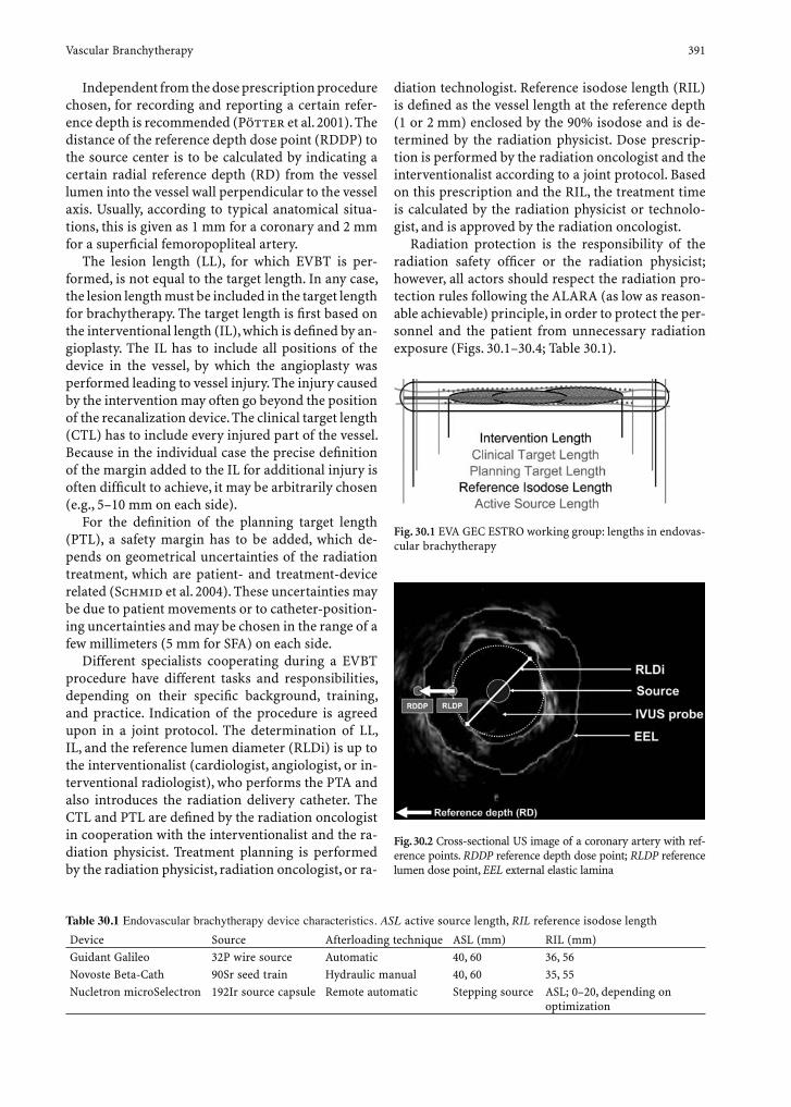
Vascular Branchytherapy 391

Independent from the dose prescription procedure chosen, for recording and reporting a certain refer-ence depth is recommended (Pötter et al. 2001). The distance of the reference depth dose point (RDDP) to the source center is to be calculated by indicating a certain radial reference depth (RD) from the vessel lumen into the vessel wall perpendicular to the vessel axis. Usually, according to typical anatomical situa-tions, this is given as 1 mm for a coronary and 2 mm for a superfi cial femoropopliteal artery.

The lesion length (LL), for which EVBT is per-formed, is not equal to the target length. In any case, the lesion length must be included in the target length for brachytherapy. The target length is fi rst based on the interventional length (IL), which is defi ned by an-gioplasty. The IL has to include all positions of the device in the vessel, by which the angioplasty was performed leading to vessel injury. The injury caused by the intervention may often go beyond the position of the recanalization device. The clinical target length (CTL) has to include every injured part of the vessel. Because in the individual case the precise defi nition of the margin added to the IL for additional injury is often diffi cult to achieve, it may be arbitrarily chosen (e.g., 5–10 mm on each side).

For the defi nition of the planning target length (PTL), a safety margin has to be added, which de-pends on geometrical uncertainties of the radiation treatment, which are patient- and treatment-device related (Schmid et al. 2004). These uncertainties may be due to patient movements or to catheter-position-ing uncertainties and may be chosen in the range of a few millimeters (5 mm for SFA) on each side.

Different specialists cooperating during a EVBT procedure have different tasks and responsibilities, depending on their specifi c background, training, and practice. Indication of the procedure is agreed upon in a joint protocol. The determination of LL, IL, and the reference lumen diameter (RLDi) is up to the interventionalist (cardiologist, angiologist, or in-terventional radiologist), who performs the PTA and also introduces the radiation delivery catheter. The CTL and PTL are defi ned by the radiation oncologist in cooperation with the interventionalist and the ra-diation physicist. Treatment planning is performed by the radiation physicist, radiation oncologist, or ra-

diation technologist. Reference isodose length (RIL) is defi ned as the vessel length at the reference depth (1 or 2 mm) enclosed by the 90% isodose and is de-termined by the radiation physicist. Dose prescrip-tion is performed by the radiation oncologist and the interventionalist according to a joint protocol. Based on this prescription and the RIL, the treatment time is calculated by the radiation physicist or technolo-gist, and is approved by the radiation oncologist.

Radiation protection is the responsibility of the radiation safety offi cer or the radiation physicist; however, all actors should respect the radiation pro-tection rules following the ALARA (as low as reason-able achievable) principle, in order to protect the per-sonnel and the patient from unnecessary radiation exposure (Figs. 30.1–30.4; Table 30.1).

Fig. 30.1 EVA GEC ESTRO working group: lengths in endovas-cular brachytherapy

Fig. 30.2 Cross-sectional US image of a coronary artery with ref-erence points. RDDP reference depth dose point; RLDP reference lumen dose point, EEL external elastic lamina

Table 30.1 Endovascular brachytherapy device characteristics. ASL active source length, RIL reference isodose length

Device Source Afterloading technique ASL (mm) RIL (mm)Guidant Galileo 32P wire source Automatic 40, 60 36, 56Novoste Beta-Cath 90Sr seed train Hydraulic manual 40, 60 35, 55Nucletron microSelectron 192Ir source capsule Remote automatic Stepping source ASL; 0–20, depending on

optimization

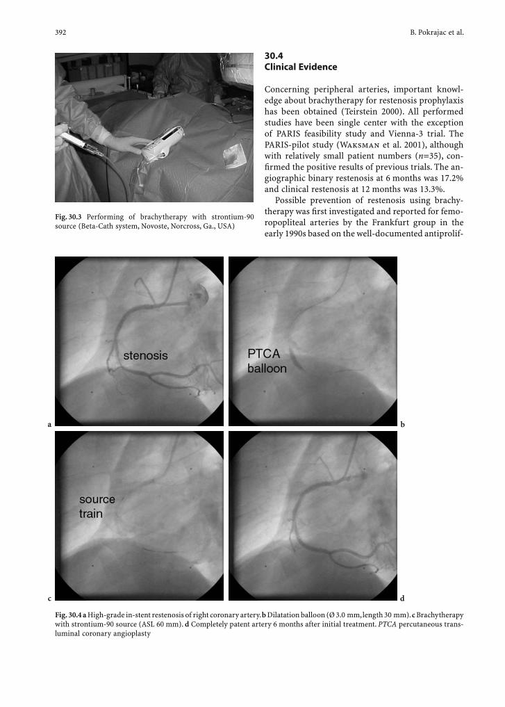
392 B. Pokrajac et al.

30.4 Clinical Evidence

Concerning peripheral arteries, important knowl-edge about brachytherapy for restenosis prophylaxis has been obtained (Teirstein 2000). All performed studies have been single center with the exception of PARIS feasibility study and Vienna-3 trial. The PARIS-pilot study (Waksman et al. 2001), although with relatively small patient numbers (n=35), con-fi rmed the positive results of previous trials. The an-giographic binary restenosis at 6 months was 17.2% and clinical restenosis at 12 months was 13.3%.

Possible prevention of restenosis using brachy-therapy was fi rst investigated and reported for femo-ropopliteal arteries by the Frankfurt group in the early 1990s based on the well-documented antiprolif-

Fig. 30.3 Performing of brachytherapy with strontium-90 source (Beta-Cath system, Novoste, Norcross, Ga., USA)

Fig. 30.4 a High-grade in-stent restenosis of right coronary artery. b Dilatation balloon (Ø 3.0 mm, length 30 mm). c Brachytherapy with strontium-90 source (ASL 60 mm). d Completely patent artery 6 months after initial treatment. PTCA percutaneous trans-luminal coronary angioplasty

b

d

a

c

Vascular Branchytherapy 393

erative effect of low dose of ionizing radiation in the prevention of keloids. Excellent results from a clini-cal phase-I/II trial in a limited number of patients (n=28) were reported, even after a long follow-up period (6 years), with a binary restenosis rate of 23% (Böttcher et al. 1994; Schopohl et al. 1996).

Vienna-2 (Pokrajac et al. 2000) was a prospective, randomized trial comparing PTA vs PTA + brachy-therapy for non-stented lesions. A total of 113 patients with claudication or critical limb ischemia having de-novo lesions of 5 cm, i.e., recurrent lesions after former PTA of any length were included. In this study stenting was not allowed. The mean PTA length was 16.7 cm in brachytherapy cohort vs 14.8 cm in pla-cebo cohort. A well-balanced patient distribution was achieved for the criteria used for stratifi cation ("de-novo stenosis vs recurrence after former PTA," "stenosis vs occlusion," "claudication vs critical limb ischemia," and "diabetes vs non-diabetes"). The dose of 12 Gray (Gy) was the same as in Frankfurt study and has been targeted at 3-mm distance from the iridium source. Primary end point was femoropopliteal patency after 6 months. Crude restenosis rate at 6 months was in the placebo arm 54 vs 28% in brachytherapy arm. Actuarial estimate of the patency rate was at 6 months 45 vs 72%, respectively. The cumulative patency rates at 12 months were 64% in brachytherapy group vs 35% in placebo group. The comparison of restenosis rates for the different subgroups with risk factors (re-currence after former PTA, occlusion and PTA length >10 cm) showed signifi cant decrease of the restenosis rate, if brachytherapy was added. Signifi cant reduction was not achieved in diabetics.

The Vienna-4 study (Wolfram et al. 2001) using brachytherapy after PTA + stenting because of unsat-isfactory angioplasty (>30% residual stenosis; mul-tiple dissections) was performed with a dose of 14 Gy prescribed 2 mm from the centering catheter surface. The antiplatelet therapy with clopidogrel was given for 1 month 75 mg/die. Binary restenosis of 30% was observed after 6 months follow-up in 33 patients.

The Vienna-3 multicenter trial (Pokrajac et al. 2003) compared PTA vs PTA followed by brachyther-apy using centering radiation delivery catheter without stenting in de-novo and restenotic lesions. The binary restenosis rate at 12 months was 23.4% in the brachy-therapy and 53.3% in the placebo group (p<0.05). The cumulative patency rates after 24 months were 77% in the brachytherapy and 39% in the placebo group (p<0.001). Late thrombosis was not seen.

The Vienna-5 study has investigated angioplasty plus stenting vs angioplasty plus stenting and addi-tional brachytherapy.

There have been several trials in coronary brachy-therapy since the mid-1990s. Many of them were dou-ble-blind randomized prospective trials, preceded by feasibility studies and followed by registry trials. Results reported thus far refer to far more than 1000 patients and focus mainly on the overall therapeutic effect of vascular brachytherapy.

The double-blind randomized trials based on iridium-192 brachytherapy (manual loading) all have revealed for lesion lengths <50 mm a signifi cant an-giographic reduction in restenosis rate at 6 months follow-up; the most outstanding of them are the fol-lowing:• SCRIPPS I (Teirstein et al. 1997) single center:

restenotic native coronary arteries or saphenous venous grafts (SVG) in 55 patients from 54 to 17%, reduction rate of 68%

• GAMMA I (Leon et al. 2001) multicenter: in-stent restenosis of coronary arteries in 252 patients from 56 to 34% WRIST (single center): in-stent restenosis of coronary arteries and SVG in 130 patients from 58 to 19%, reduction rate of 67%The clinical outcome was also signifi cantly im-

proved; however, the difference was mostly somewhat less pronounced. Clinical outcome was measured by major adverse cardiac events (MACE), which includes the need for target lesion and vessel revascularization and myocardial infarction.

For intravascular brachytherapy based on beta sources the results reported in the early experience have been less favorable. The fi rst Geneva study proved feasi-bility using the Schneider-Sauerwein-Boston Scientifi c System (yttrium-90, centering balloons) but showed no apparent effectiveness in de-novo lesions (Popowski et al. 1996). The recent multicenter Geneva dose-fi nd-ing study (Verin et al. 2001) revealed a signifi cant re-duction of restenosis rate from 9, 12, 15 to 18 Gy from 27.5, 17.5, 15.8 to 8.3% (de-novo lesions, 183 patients). The START trial (Suntharalingam et al. 2002) was the fi rst to show a signifi cant reduction in angiographic and clinical restenosis rate based on beta radiation with the Novoste system (strontium-90) from 45 to 29% and from 24 to 16%, respectively. Interesting in this analysis is that, for the fi rst time in coronary brachytherapy, a more systematic analysis for the different lengths has been performed. Looking at the vessel segment, which received the therapeutic dose, the results in this study are even more favorable. In the INHIBIT (Waksman et al. 2002) trial (in-stent restenosis, 332 patients, Guidant system, phosphorus-32) restenosis rate was dropped from 52% in placebo cohort to 26% in brachytherapy cohort for the whole analyzed segment.

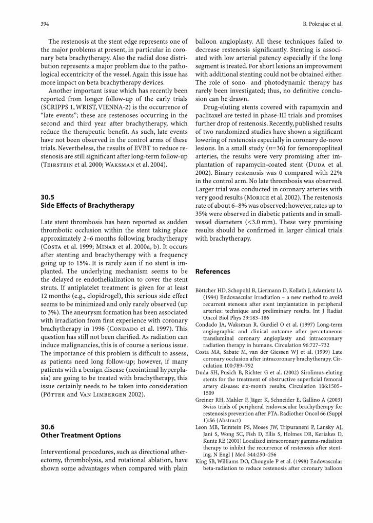
394 B. Pokrajac et al.

The restenosis at the stent edge represents one of the major problems at present, in particular in coro-nary beta brachytherapy. Also the radial dose distri-bution represents a major problem due to the patho-logical eccentricity of the vessel. Again this issue has more impact on beta brachytherapy devices.

Another important issue which has recently been reported from longer follow-up of the early trials (SCRIPPS 1, WRIST, VIENNA-2) is the occurrence of “late events”; these are restenoses occurring in the second and third year after brachytherapy, which reduce the therapeutic benefi t. As such, late events have not been observed in the control arms of these trials. Nevertheless, the results of EVBT to reduce re-stenosis are still signifi cant after long-term follow-up (Teirstein et al. 2000; Waksman et al. 2004).

30.5 Side Eff ects of Brachytherapy

Late stent thrombosis has been reported as sudden thrombotic occlusion within the stent taking place approximately 2–6 months following brachytherapy (Costa et al. 1999; Minar et al. 2000a, b). It occurs after stenting and brachytherapy with a frequency going up to 15%. It is rarely seen if no stent is im-planted. The underlying mechanism seems to be the delayed re-endothelialization to cover the stent struts. If antiplatelet treatment is given for at least 12 months (e.g., clopidrogel), this serious side effect seems to be minimized and only rarely observed (up to 3%). The aneurysm formation has been associated with irradiation from fi rst experience with coronary brachytherapy in 1996 (Condado et al. 1997). This question has still not been clarifi ed. As radiation can induce malignancies, this is of course a serious issue. The importance of this problem is diffi cult to assess, as patients need long follow-up; however, if many patients with a benign disease (neointimal hyperpla-sia) are going to be treated with brachytherapy, this issue certainly needs to be taken into consideration (Pötter and Van Limbergen 2002).

30.6 Other Treatment Options

Interventional procedures, such as directional ather-ectomy, thrombolysis, and rotational ablation, have shown some advantages when compared with plain

balloon angioplasty. All these techniques failed to decrease restenosis signifi cantly. Stenting is associ-ated with low arterial patency especially if the long segment is treated. For short lesions an improvement with additional stenting could not be obtained either. The role of sono- and photodynamic therapy has rarely been investigated; thus, no defi nitive conclu-sion can be drawn.

Drug-eluting stents covered with rapamycin and paclitaxel are tested in phase-III trials and promises further drop of restenosis. Recently, published results of two randomized studies have shown a signifi cant lowering of restenosis especially in coronary de-novo lesions. In a small study (n=36) for femoropopliteal arteries, the results were very promising after im-plantation of rapamycin-coated stent (Duda et al. 2002). Binary restenosis was 0 compared with 22% in the control arm. No late thrombosis was observed. Larger trial was conducted in coronary arteries with very good results (Morice et al. 2002). The restenosis rate of about 6–8% was observed; however, rates up to 35% were observed in diabetic patients and in small-vessel diameters (<3.0 mm). These very promising results should be confi rmed in larger clinical trials with brachytherapy.

References

Böttcher HD, Schopohl B, Liermann D, Kollath J, Adamietz IA (1994) Endovascular irradiation – a new method to avoid recurrent stenosis after stent implantation in peripheral arteries: technique and preliminary results. Int J Radiat Oncol Biol Phys 29:183–186

Condado JA, Waksman R, Gurdiel O et al. (1997) Long-term angiographic and clinical outcome after percutaneous transluminal coronary angioplasty and intracoronary radiation therapy in humans. Circulation 96:727–732

Costa MA, Sabate M, van der Giessen WJ et al. (1999) Late coronary occlusion after intracoronary brachytherapy. Cir-culation 100:789–792

Duda SH, Pusich B, Richter G et al. (2002) Sirolimus-eluting stents for the treatment of obstructive superfi cial femoral artery disease: six-month results. Circulation 106:1505–1509

Greiner RH, Mahler F, Jäger K, Schneider E, Gallino A (2003) Swiss trials of peripheral endovascular brachytherapy for restenosis prevention after PTA. Radiother Oncol 66 (Suppl 1):S6 (Abstract)

Leon MB, Teirstein PS, Moses JW, Tripuraneni P, Lansky AJ, Jani S, Wong SC, Fish D, Ellis S, Holmes DR, Keriakes D, Kuntz RE (2001) Localized intracoronary gamma-radiation therapy to inhibit the recurrence of restenosis after stent-ing. N Engl J Med 344:250–256

King SB, Williams DO, Chougule P et al. (1998) Endovascular beta-radiation to reduce restenosis after coronary balloon

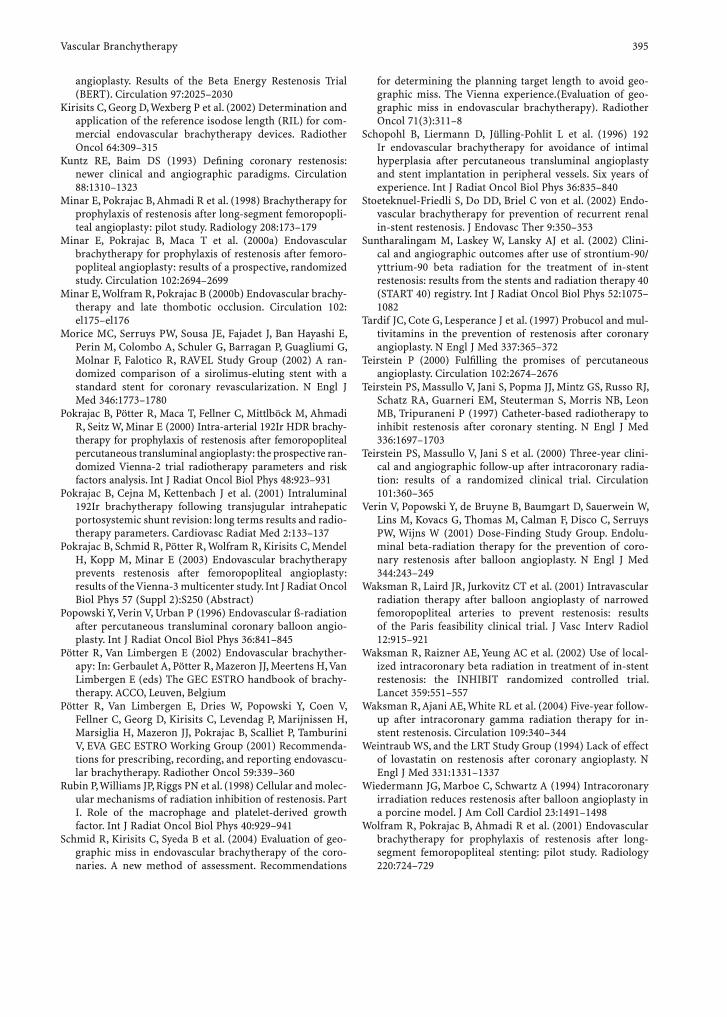
Vascular Branchytherapy 395

angioplasty. Results of the Beta Energy Restenosis Trial (BERT). Circulation 97:2025–2030

Kirisits C, Georg D, Wexberg P et al. (2002) Determination and application of the reference isodose length (RIL) for com-mercial endovascular brachytherapy devices. Radiother Oncol 64:309–315

Kuntz RE, Baim DS (1993) Defi ning coronary restenosis: newer clinical and angiographic paradigms. Circulation 88:1310–1323

Minar E, Pokrajac B, Ahmadi R et al. (1998) Brachytherapy for prophylaxis of restenosis after long-segment femoropopli-teal angioplasty: pilot study. Radiology 208:173–179

Minar E, Pokrajac B, Maca T et al. (2000a) Endovascular brachytherapy for prophylaxis of restenosis after femoro-popliteal angioplasty: results of a prospective, randomized study. Circulation 102:2694–2699

Minar E, Wolfram R, Pokrajac B (2000b) Endovascular brachy-therapy and late thombotic occlusion. Circulation 102:el175–el176

Morice MC, Serruys PW, Sousa JE, Fajadet J, Ban Hayashi E, Perin M, Colombo A, Schuler G, Barragan P, Guagliumi G, Molnar F, Falotico R, RAVEL Study Group (2002) A ran-domized comparison of a sirolimus-eluting stent with a standard stent for coronary revascularization. N Engl J Med 346:1773–1780

Pokrajac B, Pötter R, Maca T, Fellner C, Mittlböck M, Ahmadi R, Seitz W, Minar E (2000) Intra-arterial 192Ir HDR brachy-therapy for prophylaxis of restenosis after femoropopliteal percutaneous transluminal angioplasty: the prospective ran-domized Vienna-2 trial radiotherapy parameters and risk factors analysis. Int J Radiat Oncol Biol Phys 48:923–931

Pokrajac B, Cejna M, Kettenbach J et al. (2001) Intraluminal 192Ir brachytherapy following transjugular intrahepatic portosystemic shunt revision: long terms results and radio-therapy parameters. Cardiovasc Radiat Med 2:133–137

Pokrajac B, Schmid R, Pötter R, Wolfram R, Kirisits C, Mendel H, Kopp M, Minar E (2003) Endovascular brachytherapy prevents restenosis after femoropopliteal angioplasty: results of the Vienna-3 multicenter study. Int J Radiat Oncol Biol Phys 57 (Suppl 2):S250 (Abstract)

Popowski Y, Verin V, Urban P (1996) Endovascular ß-radiation after percutaneous transluminal coronary balloon angio-plasty. Int J Radiat Oncol Biol Phys 36:841–845

Pötter R, Van Limbergen E (2002) Endovascular brachyther-apy: In: Gerbaulet A, Pötter R, Mazeron JJ, Meertens H, Van Limbergen E (eds) The GEC ESTRO handbook of brachy-therapy. ACCO, Leuven, Belgium

Pötter R, Van Limbergen E, Dries W, Popowski Y, Coen V, Fellner C, Georg D, Kirisits C, Levendag P, Marijnissen H, Marsiglia H, Mazeron JJ, Pokrajac B, Scalliet P, Tamburini V, EVA GEC ESTRO Working Group (2001) Recommenda-tions for prescribing, recording, and reporting endovascu-lar brachytherapy. Radiother Oncol 59:339–360

Rubin P, Williams JP, Riggs PN et al. (1998) Cellular and molec-ular mechanisms of radiation inhibition of restenosis. Part I. Role of the macrophage and platelet-derived growth factor. Int J Radiat Oncol Biol Phys 40:929–941

Schmid R, Kirisits C, Syeda B et al. (2004) Evaluation of geo-graphic miss in endovascular brachytherapy of the coro-naries. A new method of assessment. Recommendations

for determining the planning target length to avoid geo-graphic miss. The Vienna experience.(Evaluation of geo-graphic miss in endovascular brachytherapy). Radiother Oncol 71(3):311–8

Schopohl B, Liermann D, Jülling-Pohlit L et al. (1996) 192 Ir endovascular brachytherapy for avoidance of intimal hyperplasia after percutaneous transluminal angioplasty and stent implantation in peripheral vessels. Six years of experience. Int J Radiat Oncol Biol Phys 36:835–840

Stoeteknuel-Friedli S, Do DD, Briel C von et al. (2002) Endo-vascular brachytherapy for prevention of recurrent renal in-stent restenosis. J Endovasc Ther 9:350–353

Suntharalingam M, Laskey W, Lansky AJ et al. (2002) Clini-cal and angiographic outcomes after use of strontium-90/ yttrium-90 beta radiation for the treatment of in-stent restenosis: results from the stents and radiation therapy 40 (START 40) registry. Int J Radiat Oncol Biol Phys 52:1075–1082

Tardif JC, Cote G, Lesperance J et al. (1997) Probucol and mul-tivitamins in the prevention of restenosis after coronary angioplasty. N Engl J Med 337:365–372

Teirstein P (2000) Fulfi lling the promises of percutaneous angioplasty. Circulation 102:2674–2676

Teirstein PS, Massullo V, Jani S, Popma JJ, Mintz GS, Russo RJ, Schatz RA, Guarneri EM, Steuterman S, Morris NB, Leon MB, Tripuraneni P (1997) Catheter-based radiotherapy to inhibit restenosis after coronary stenting. N Engl J Med 336:1697–1703

Teirstein PS, Massullo V, Jani S et al. (2000) Three-year clini-cal and angiographic follow-up after intracoronary radia-tion: results of a randomized clinical trial. Circulation 101:360–365

Verin V, Popowski Y, de Bruyne B, Baumgart D, Sauerwein W, Lins M, Kovacs G, Thomas M, Calman F, Disco C, Serruys PW, Wijns W (2001) Dose-Finding Study Group. Endolu-minal beta-radiation therapy for the prevention of coro-nary restenosis after balloon angioplasty. N Engl J Med 344:243–249

Waksman R, Laird JR, Jurkovitz CT et al. (2001) Intravascular radiation therapy after balloon angioplasty of narrowed femoropopliteal arteries to prevent restenosis: results of the Paris feasibility clinical trial. J Vasc Interv Radiol 12:915–921

Waksman R, Raizner AE, Yeung AC et al. (2002) Use of local-ized intracoronary beta radiation in treatment of in-stent restenosis: the INHIBIT randomized controlled trial. Lancet 359:551–557

Waksman R, Ajani AE, White RL et al. (2004) Five-year follow-up after intracoronary gamma radiation therapy for in-stent restenosis. Circulation 109:340–344

Weintraub WS, and the LRT Study Group (1994) Lack of effect of lovastatin on restenosis after coronary angioplasty. N Engl J Med 331:1331–1337

Wiedermann JG, Marboe C, Schwartz A (1994) Intracoronary irradiation reduces restenosis after balloon angioplasty in a porcine model. J Am Coll Cardiol 23:1491–1498

Wolfram R, Pokrajac B, Ahmadi R et al. (2001) Endovascular brachytherapy for prophylaxis of restenosis after long-segment femoropopliteal stenting: pilot study. Radiology 220:724–729

Partial Breast Brachytherapy After Conservative Surgery for Early Breast Cancer: Techniques and Results 397

31 Partial Breast Brachytherapy After Conservative Surgery for Early Breast Cancer: Techniques and Results Yazid Belkacémi, Jean-Michel Hannoun-Lévi, and Eric Lartigau

Y. Belkacémi, MD, PhD; E. Lartigau, MD, PhDDepartment of Radiation Oncology, Centre Oscar Lambret, University of Lille II, 3 rue Frédéric Combemale, 59020 Lille, FranceJ.-M. Hannoun-Lévi, MD, PhDDepartment of Radiation Oncology, Centre Antoine Lacassagne, 33 avenue de Valombrose, 06189 Nice Cedex, France

31.1 Introduction

Post-operative radiation therapy (RT) has been shown in a number of randomized trials to reduce the risk of breast cancer recurrence following breast-conserv-ing surgery (Clark 1992; Forrest 1996; Liljegren 1994; Fisher 2002; Veronesi 2002).

Breast-conserving surgery, adjuvant postoperative RT, and systemic therapy has become standard treat-ment for increasing numbers of women with early breast cancer. Although breast-conserving therapy has become an accepted alternative for early-stage breast cancer patients, a number of studies show that only 10–70% of patients qualifying for brachy-therapy actually receive it in North America. In an

CONTENTS

31.1 Introduction 39731.2 Interstitial Brachytherapy in Partial Breast Irradiation 39831.2.1 Technique 39831.2.2 Partial Breast Irradiation Using Low-Dose-Rate Interstitial Brachytherapy 39931.2.3 Partial Breast Irradiation Using High-Dose-Rate Interstitial Brachytherapy 40131.3 Brachytherapy Using MammoSite Balloon Device for Partial Breast Irradiation 40231.3.1 MammoSite Device Insertion Procedure After Conservative Surgery 40231.3.2 Dosimetric Aspects 40331.3.3 Acute Toxicity 40431.3.4 Late Effects, Cosmetic Results, and Local Control 40431.4 Conclusion 405 References 405

effort to overcome this problem, a number of cen-ters have attempted an accelerated regimen using interstitial brachytherapy as the sole radiation mo-dality (Clarke 1994; Fentiman 1991; Kuske and Bolton1995; Perera 1995, 1997; Vicini 1997, 1999). This treatment approach has the potential to make brachytherapy more attractive to many patients, and poses fewer logistic problems. Moreover, in some patients older than 65 years with or without co-mor-bidities, the long duration of conventional fraction-ated RT may signifi cantly alter the quality of life and the treatment observance. Ballard-Barbash et al. (1996) found among a cohort 18704 patients aged 65 years or older that the receipt of postoperative RT declined substantially with age, irrespective of co-morbidity and disease stage. For the age groups 65–69 and 80 years or older, the use of irradiation felt from 77 to 24% in women without co-morbid condi-tions and 50–12% with two or more co-morbid con-ditions. For elderly women, with the low risk of lo-cal recurrence, accelerated partial breast irradiation during 6 weeks (one fraction per week) seems to be also a reasonable alternative to compare in the future to post-operative standard whole-breast radiation therapy (WBRT; Hannoun-Lévi 2003).

After conservative surgery, WBRT is the stan-dard of care. The RT schedule consists of delivering 45–50 Gy to the whole breast, in 4.5–5 weeks, fol-lowed by a boost dose of 10–20 Gy to the tumor bed. Brachytherapy is used in this setting as one of the boost techniques. The rational for elective treatment of the whole breast after conservative surgery stems from the fi ndings of pathological studies of mas-tectomy specimens in women with localized breast cancer and from preoperative radiological imaging of patients selected for conservative surgery, which demonstrated the existence of unsuspected foci of carcinoma in 16–37% of women (Rosen 1975; Orel 1995; Moon 2002). This fi nding initially led to the notion that breast-conserving therapy was an inap-propriate treatment option for women with early-stage disease; however, the type and location of local recurrences in studies of standard breast-conserving

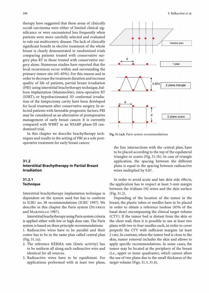
398 Y. Belkacémi et al.

therapy have suggested that these areas of clinically occult carcinoma were either of limited clinical sig-nifi cance or were encountered less frequently when patients were more carefully selected and evaluated to rule out multicentric disease. The lack of clinically signifi cant benefi t in elective treatment of the whole breast is clearly demonstrated in randomized trials comparing patients treated with conservative sur-gery plus RT to those treated with conservative sur-gery alone. Numerous studies have reported that the local recurrences occur within and surrounding the primary tumor site (65–85%). For this reason and in order to decrease the treatment duration and increase quality of life of patients, partial breast irradiation (PBI) using interstitial brachytherapy technique, bal-loon implantation (MammoSite), intra-operative RT (IORT), or hypofractionated 3D conformal irradia-tion of the lumpectomy cavity have been developed for local treatment after conservative surgery. In se-lected patients with favorable prognostic factors, PBI may be considered as an alternative of postoperative management of early breast cancer. It is currently compared with WBRT in an NSABP phase-III ran-domized trial.

In this chapter we describe brachytherapy tech-niques and results in the setting of PBI as a sole post-operative treatment for early breast cancer.

31.2 Interstitial Brachytherapy in Partial Breast Irradiation

31.2.1 Technique

Interstitial brachytherapy implantation technique is dependent on the system used but has to conform to ICRU no. 58 recommendations (ICRU 1997). We describe in this chapter the Paris system (Dutreix and Marinello 1987).

Interstitial brachytherapy using Paris system criteria is applied either with low or high dose rate. The Paris system is based on three principle recommendations:1. Radioactive wires have to be parallel and their center has to be in the same plan called central plan (Fig. 31.1a).2. The reference KERMA rate (lineic activity) has

to be uniform all along each radioactive wire and identical for all sources.

3. Radioactive wires have to be equidistant. For applications performed with at least two plans,

the line intersections with the central plan, have to be placed according to the top of the equilateral triangles or scares (Fig. 31.1b). In case of triangle application, the spacing between the different plans is equal to the spacing between radioactive wires multiplied by 0.87.

In order to avoid acute and late skin side effects, the application has to respect at least 5-mm margin between the iridium-192 wires and the skin surface (Fig. 31.2).

Depending of the location of the tumor in the breast, the plastic tubes or needles have to be placed in order to obtain a reference isodose (85% of the basal dose) encompassing the clinical target volume (CTV). If the tumor bed is distant from the skin or the chest wall, then it is possible to use at least two plans with two to four needles each, in order to cover properly the CTV with suffi cient margins (at least 2 cm). In contrast, when the tumor bed is close to the skin, tumor removal includes the skin and allows to apply specifi c recommendations. In some cases, the tumor may be located at the periphery of the breast (i.e., upper or inner quadrants), which cannot allow the use of two plans due to the small thickness of the target volume (Figs. 31.3, 31.4).

Fig. 31.1a,b. Paris system recommendations

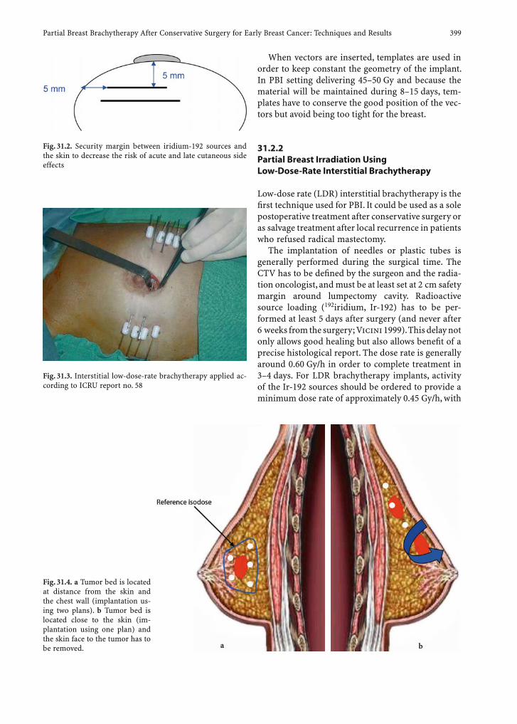
Partial Breast Brachytherapy After Conservative Surgery for Early Breast Cancer: Techniques and Results 399

When vectors are inserted, templates are used in order to keep constant the geometry of the implant. In PBI setting delivering 45–50 Gy and because the material will be maintained during 8–15 days, tem-plates have to conserve the good position of the vec-tors but avoid being too tight for the breast.

31.2.2 Partial Breast Irradiation Using Low-Dose-Rate Interstitial Brachytherapy

Low-dose rate (LDR) interstitial brachytherapy is the fi rst technique used for PBI. It could be used as a sole postoperative treatment after conservative surgery or as salvage treatment after local recurrence in patients who refused radical mastectomy.

The implantation of needles or plastic tubes is generally performed during the surgical time. The CTV has to be defi ned by the surgeon and the radia-tion oncologist, and must be at least set at 2 cm safety margin around lumpectomy cavity. Radioactive source loading (192iridium, Ir-192) has to be per-formed at least 5 days after surgery (and never after 6 weeks from the surgery; Vicini 1999). This delay not only allows good healing but also allows benefi t of a precise histological report. The dose rate is generally around 0.60 Gy/h in order to complete treatment in 3–4 days. For LDR brachytherapy implants, activity of the Ir-192 sources should be ordered to provide a minimum dose rate of approximately 0.45 Gy/h, with

Fig. 31.2. Security margin between iridium-192 sources and the skin to decrease the risk of acute and late cutaneous side effects

Fig. 31.3. Interstitial low-dose-rate brachytherapy applied ac-cording to ICRU report no. 58

Fig. 31.4. a Tumor bed is located at distance from the skin and the chest wall (implantation us-ing two plans). b Tumor bed is located close to the skin (im-plantation using one plan) and the skin face to the tumor has to be removed. ba

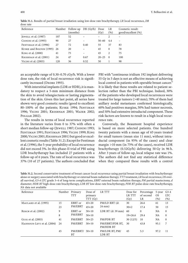
400 Y. Belkacémi et al.

an acceptable range of 0.30–0.70 cGy/h. With a lower dose rate, the risk of local recurrence risk is signifi -cantly increased (Deore 1993).

With interstitial implants (LDR or HDR), it is man-datory to respect a 5-mm minimum distance from the skin to avoid telangiectasia or lasting pigmenta-tion of the skin. Given this last point, all series have shown very good cosmetic results (good to excellent: 80–100% of the patients; Kuske 1994; Fentiman 1996; Vicini 2001; Krishnan 2001; Wazer 2002; Polgar 2002).

The results in terms of local recurrence reported in the literature varies from 0 to 37% with often a short median follow-up (Jewell 1987; Cionini 1993; Fentiman 1991; Fentiman 1996; Vicini 1999; King 2000; Vicini 2001; Krishnan 2001) but good or excel-lent cosmetic results (Table 31.2). Except for Fentiman et al. (1996), the 5-year probability of local recurrence did not exceed 5%. In this phase-II trial of PBI using LDR brachytherapy has included 27 patients with a follow-up of 6 years. The rate of local recurrence was 37% (10 of 27 patients). The authors concluded that

PBI with “continuous iridium 192 implant delivering 55 Gy in 5 days is not an effective means of achieving local control in patients with operable breast cancer.” It is likely that these results are related to patient se-lection rather than the PBI technique. Indeed, 30% of the patients who developed local recurrences were treated for large tumors (>40 mm); 70% of them had axillary nodal metastases confi rmed histologically, 60% had positives margins, 50% had tumor necrosis, and 50% had extensive intraductal component. These risk factors are known to result in a high local recur-rence rate.

Conversely, the Beaumont hospital experience is based on more selected patients. One hundred twenty patients with a mean age of 65 years treated for small tumors (mean size 11 mm), without intra-ductal component (in 95% of the cases) and clear margin >10 mm (in 75% of the cases), received LDR brachytherapy (0.52Gy/h) delivering 50 Gy in 96 h. After 3 years of follow-up, local relapse rate was 1%. The authors did not fi nd any statistical difference when they compared these results with a control

Table 31.1. Results of partial breast irradiation using low-dose rate brachytherapy. LR local recurrence, DR dose rate

Reference Number Follow-up (months)

DR (Gy/h) Dose (Gy)

LR (%)

Cosmetic result: good/excellent (%)

Jewell et al. (1987) 107 52 – – 2 –Cionini et al. (1993) 90 27 – 50–60 4.4 –Fentiman et al. (1996) 27 72 0.40 55 37 83Kuske and Bolton (1995) 26 20 – 45 0 78King et al. (2000) 41 75 – 45 2 75Krishnan et al. (2001) 24 47 0.67 20–25 0 100Vicini et al. (2003) 120 36 0.52 50 1 98

Table 31.2. Second conservative treatment of breast cancer local recurrence using partial breast irradiation with brachytherapy alone or surgery associated with brachytherapy or external beam radiation therapy. TTT treatment, LR local recurrence, OS over-all survival, G3-4 LTC grade 3–4 of long-term complications, EBRT external beam radiation therapy, PM partial mastectomy, d diameter; HDR BT high-dose-rate brachytherapy, LDR BT low-dose-rate brachytherapy, PDR BT pulse-dose-rate brachytherapy, NA data not available

Reference Number Primary TTT

Dose of primary TTT (Gy)

LR TTT Dose for LR TTT (Gy)

Percentage of second LR

5-year OS (%)

G3-4 LTC (%)

Maulard et al. (1995) 15 EBRT or PM/EBRT

45+20 PM/LD RBT (d: 24 mm)

30 26.6 61 1323 45+20 30×2 17.4 50 15

Resch et al. (2002) 9 EBRT or PM/EBRT

50+10 LDR BT (d: 39 mm) 60 0 NA 08 50+10 19+26.6 29.4 NA 0

Guix et al. (2003) 41 PM/EBRT 50+25 PM/PDR BT 30 (12/5) 10 NA 0Hannoun-Levi et al. (2004) 24 PM/EBRT 50+10 PM/EBRT/PDR BT,

PM/HDR BT30 43.8 95.1 7

45 PM/EBRT/BT

50+10 PM/LDR BT, PM/LDR BT

45 5.3 97.2 11

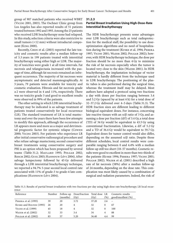
Partial Breast Brachytherapy After Conservative Surgery for Early Breast Cancer: Techniques and Results 401

group of 907 matched patients who received WBRT (Vicini 2001, 2003). The Oschner Clinic group from Los Angeles has also reported results of 51 patients treated between 1992 and 1993. Among the 25 patients who received LDR brachytherapy none had relapsed. In this study, selection criteria were also restrictive to small tumors (<12 mm) without intraductal compo-nent (King 2000).

Recently, Chen et al. (2003) reported the late tox-icity and cosmetic results after a median follow-up of 5.3 years in 199 patients treated with interstitial brachytherapy using either high or LDR. The major-ity of toxicities were grade 1 at all time intervals. Fat necrosis and telangiectasia increased with the pas-sage of time, although fat necrosis remained an infre-quent occurrence. The majority of fat necroses were asymptomatic and detected mammographically. At 5 years, 79 patients were available for toxicity and cosmetic evaluation. Fibrosis and fat necrosis grade

2 were observed in 4 and 11%, respectively. There was no toxicity grade 3 and good to excellent results were observed in 99% of the patients.

The other setting in which LDR interstitial brachy-therapy may be indicated is as salvage treatment of patients treated conservatively for local recurrence (LR). The standard treatment of LR is total mastec-tomy and over the years there have been few attempts to modify this approach, although the occurrence of LR appears more and more as a major and detrimen-tal prognostic factor for systemic relapse (Cowen 2000; Vicini 2003). For patients who experience LR after initial conservative radiosurgical procedure and who refuse salvage mastectomy, second conservative breast treatments using conservative surgery and PBI is an option which has been proposed by several teams (Table 31.2; Maulard 1995; Polgar 2002; Resch 2002; Guix 2003; Hannoun-Lévi 2004). After salvage lumpectomy followed by 45 Gy delivered through a LDR interstitial brachytherapy technique, we reported a 94.7% 5-year second local control rate associated with 11% of grade-3 to grade-4 late com-plications (Hannoun-Lévi 2004).

31.2.3 Partial Breast Irradiation Using High-Dose-Rate Interstitial Brachytherapy

The HDR brachytherapy presents some advantages over LDR brachytherapy such as total radioprotec-tion for the medical staff, the possibility to use dose-optimization algorithms and no need of hospitaliza-tion during the treatment (Kuske et al. 1994; Perera 1997; Vicini 2001; Wazer 2002; Polgar 2002); how-ever, with HDR brachytherapy technique, the dose per fraction should be no more than 4 Gy to minimize the risk of fat necrosis especially when the tumor is located very close to the skin (Wazer 2001). In HDR brachytherapy, the implantation technique of vector material is hardly different from the technique used in LDR brachytherapy. The positioning of the plas-tic tubes is also performed during the surgical time, whereas the treatment itself may be delayed. Most authors have adopted a protocol using two fractions a day with doses per fraction ranging between 3.4 and 5.2 Gy (spaced by at least 6 h) for a total dose of 32–37.2 Gy delivered over 4–5 days (Table 31.3). The HDR fraction sizes are different leading to different biological equivalent doses. For instance, concerning late reactive tissues with an / ratio of 3 Gy, and as-suming a dose per fraction (d/f) of 3.4 Gy, a total dose (TD) of 34 Gy would be equivalent to 43.5 Gy using conventional fractionation. Likewise, a d/f of 5.2 Gy and a TD of 36.4 Gy would be equivalent to 59.7 Gy. Equivalent doses for tumor control would also differ, depending on the assumed / ratio. Despite those different schedules, local control results were com-parable ranging between 0 and 4.4% with a median follow-up still too short (18–57 months). Cosmetic re-sults were good to excellent in more than two-thirds of the patients (Kuske 1994; Perera 1997; Vicini 2001; Polgar 2002). Wazer et al. (2001) described a high rate of fat necrosis (58%) after a median follow-up of 24 months, depending on the dose rate. This com-plication was most likely caused by a combination of surgical and radiation parameters. Indeed, the risk of

Table 31.3. Results of partial breast irradiation with two fractions per day using high-dose rate brachytherapy. LR local recur-rence

Reference Number Follow-up (months)

Dose/fraction (Gy)

Total dose (Gy)

LR (%)

Cosmetic results good/excellent (%)

Perera et al. (1995) 39 20 3.72 37.20 2.6 –Kuske and Bolton (1995) 26 20 4 32 0 67Vicini et al. (1999) 45 18 4 32 0 100Wazer et al. (2002) 32 33 3.4 34 4 88Polgar et al. (2002) 83 57 5.20 36.40 4.4 99

402 Y. Belkacémi et al.

grade-3 or grade-4 toxicity was associated exclusively with the volume of the implant as refl ected in the number of source dwell positions and volume of tis-sue exposed to fractional doses of 34 Gy (100%), 51 Gy (150%), and 68 Gy (200%). The authors postulated that complication risk may be more closely related to the volume of tissue encompassed within 150% isodose shell. This is suggested by the fact that the lower inci-dence of complications are observed when the median values are limited like in the William Beaumont (me-dian 26.4 cm3, range 15.5–38.8 cm3) and in the Tufts/Brown (median 37 cm3, range 14–144 cm3) studies.

Recently, Shah et al. (2003) reported toxicity and cosmetic outcome of 141 patients treated for early breast cancer with HDR brachytherapy delivering 32–34 Gy over 4 or 5 days to the lumpectomy cavity with a 2-cm margin. During treatment 15% of the patients experienced a grade-1 skin reaction. The most com-mon toxicity was pockmarks (i.e., discoloration of the skin at the entry and exit sites of the brachytherapy catheters), which became less noticeable with each subsequent follow-up visit. At 12 months, 98% of the patients had an excellent or good cosmetic outcome.

31.3 Brachytherapy Using MammoSite Balloon Device for Partial Breast Irradiation

Although the principle of brachytherapy as a sole ra-diation modality may be adopted for selected patients, the optimal technique to deliver radiation has to be investigated more thoroughly. Interstitial brachyther-apy seems to be less trivial to deliver (Fentiman 1996; Vicini 1999; Kestin 2000) and is not available and therefore not adopted in many centers. To make brachy-therapy more accessible, a new breast treatment device (MammoSite RTS; Proxima Therapeutics, Alpharetta, Ga.) has recently been developed (Fig. 31.5). This device delivers a high dose rate at the center of an infl ated bal-loon that is placed intra-operatively (or days following surgery) into the lumpectomy cavity.

In this section we describe the surgical procedure for MammoSite insertion, dosimetric aspects, and results.

31.3.1 MammoSite Device Insertion Procedure After Conservative Surgery

The MammoSite device consists of a catheter with a silicone balloon and a shaft approximately 6 mm in

Fig. 31.5. MammoSite radiation therapy system

diameter and 15 mm in length. The shaft contains a small infl ation channel and a second larger channel for treatment after passage of the HDR source. An injection port is attached to the infl ation channel, and a luer fi tting is attached to the infl ation channel. An adapter is provided separately to connect with any brand of remote afterloading device (Fig. 31.5). In the initial phase-II studies demonstrating reliability and safety of the device, all patients had a CT scan before initiating treatment and also just before its removal at the end of treatment. Ultrasound or computed to-mography were also used to determine the critical parameters of treatment, namely balloon diameter, symmetry, conformity, and its proximity to the chest wall and skin. Before and during treatment, standard orthogonal X-rays are useful for treatment planning and verifi cation of balloon integrity.

The optimal technique and timing for the implan-tation have not been well defi ned. It is possible to in-sert the device peroperatively or utilizing percutane-ous ultrasound-guided technique. The disadvantage of the intra-operative implantation is the high rates of disqualifi ed patients (29%) for postoperative his-tology issues. In the postoperative ultrasound-guided percutaneous placement the disadvantage is related to the unfavorable balloon positioning requir-ing catheter removal. Zannis et al. (2003) reported among 23 patients implanted utilizing percutaneous ultrasound-guided technique only 2 (9%) of second-ary device removal.

We recently reported the different steps of the sur-gical procedure of lumpectomy and intra-operative implantation of the MammoSite (Belkacémi 2003). The procedure is presented in Fig. 31.6.

After sentinel node detection and removal, the MammoSite applicator implantation is preceded by a standard lumpectomy. The wide excision creates a lumpectomy cavity around which clear margins

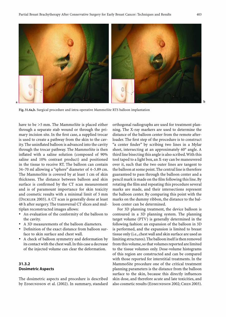
Partial Breast Brachytherapy After Conservative Surgery for Early Breast Cancer: Techniques and Results 403

have to be >5 mm. The MammoSite is placed either through a separate stab wound or through the pri-mary incision site. In the fi rst case, a supplied trocar is used to create a pathway from the skin to the cav-ity. The uninfl ated balloon is advanced into the cavity through the trocar pathway. The MammoSite is then infl ated with a saline solution (composed of 90% saline and 10% contrast product) and positioned in the tissue to receive RT. The balloon can contain 34–70 ml allowing a “sphere” diameter of 4–5.89 cm. The MammoSite is covered by at least 1 cm of skin thickness. The distance between balloon and skin surface is confi rmed by the CT scan measurement and is of paramount importance for skin toxicity and cosmetic results with a minimal limit of 5 mm (Dickler 2003). A CT scan is generally done at least 48 h after surgery. The transversal CT slices and mul-tiplan reconstructed images allows:• An evaluation of the conformity of the balloon to

the cavity.• A 3D measurements of the balloon diameters.• Defi nition of the exact distance from balloon sur-

face to skin surface and chest wall.• A check of balloon symmetry and deformation by

its contact with the chest wall. In this case a decrease of the injected volume can clear the deformation.

31.3.2 Dosimetric Aspects

The dosimetric aspects and procedure is described by Edmundson et al. (2002). In summary, standard

orthogonal radiographs are used for treatment plan-ning. The X-ray markers are used to determine the distance of the balloon center from the remote after-loader. The fi rst step of the procedure is to construct “a center fi nder” by scribing two lines in a Mylar sheet, intersecting at an approximately 60° angle. A third line bisecting this angle is also scribed. With this tool taped to a light box, an X-ray can be maneuvered over it, such that the two outer lines are tangent to the balloon at some point. The central line is therefore guaranteed to pass through the balloon center and a pencil mark is made on the fi lm following this line. By rotating the fi lm and repeating this procedure several marks are made, and their intersections represent the balloon center. By comparing this point with the marks on the dummy ribbon, the distance to the bal-loon center can be determined.

For 3D planning treatment, the device balloon is contoured in a 3D planning system. The planning target volume (PTV) is generally determined in the following fashion: an expansion of the balloon in 3D is performed, and the expansion is limited to breast tissue only (i.e., chest wall and skin surface are used as limiting structures). The balloon itself is then removed from this volume, so that volumes reported are limited to the tissue volumes only. Dose-volume histograms of this region are constructed and can be compared with those reported for interstitial treatments. In the MammoSite procedure one of the critical treatment planning parameters is the distance from the balloon surface to the skin, because this directly infl uences skin dose, and therefore acute and late toxicities, and also cosmetic results (Edmundson 2002; Chen 2003).

Fig. 31.6a,b. Surgical procedure and intra-operative MammoSite RTS balloon implantation

ba

404 Y. Belkacémi et al.

A minimum distance of 5 mm is set for the majority of the protocols in order to keep the skin dose at any point less than 150% of the prescribed dose, which is generally delivered at 1 cm around the balloon; how-ever, the minimum skin distance is not always easily determined from the transverse CT slices alone and is impossible to determine from plane fi lms. In the ini-tial clinical experience with MammoSite, Keisch et al. (2003) found that the skin–balloon surface distance and balloon-cavity conformance was the main fac-tors limiting the initial use of the device. Ineligibility for poor balloon conformance (i.e., air- or fl uid-fi lled gaps between balloon and cavity) and for limited skin–balloon surface was observed in 7 of 11 and 4 of 11 patients, respectively. The poor conformance may induce signifi cant modifi cation of the absolute tissue volumes receiving 100% (V340), 150% (V510), and 200% (V680) of the total dose of 34 Gy. There is a suggestion in a recent publication (Wazer 2001) that these values may be associated with development of toxicities such as fat necrosis.

The homogeneity index (DHI) as fi rst described by Wu et al. (1988) describes the fraction of the vol-ume of the 100% isodose surface (i.e., treated volume) that receives less than 150% of the prescribed dose. According to the initial US experience reported by Edmundson et al. (2002), the DHI with MammoSite is lower than interstitial brachytherapy, but the fi rst device is more reproducible and produced better PTV coverage (Edmundson et al. 2002). Moreover, the conformance of the balloon to the cavity wall is essential to assure appropriate dosimetry. Regarding the 9 of 34 (27%) patients requiring removal in the open setting, the reasons included mostly technical issues, such as conformance, as well as pathological issues such as nodal positivity.

Another particularity described with MammoSite is that the balloon is not perfectly symmetrical; thus, isodose distribution exhibits anisotropy because of self-absorption along the source axis. This anisotropy can be used to advantage by orienting the balloon normal to the skin when somewhat reduced margins between the balloon and skin are encountered.

Recently, Dickler et al. (2003) suggested that the volume of normal breast tissue treated by MammoSite device is comparable to other methods of interstitial brachytherapy which treat 1–2 cm margin of tissue around the excision cavity. In their study of 21 pa-tients, they compared two techniques using either a single-prescription point, single dwell position opti-mization, or a six-prescription point, multiple dwell position technique; in the latter, the six points were placed 1 cm from the balloon. Four of them were

placed in a plan transverse to the balloon axis per-pendicular to the catheter axis and two points along the axis of the catheter; the last were used to compen-sate for the decreased dose coverage due to anisotropy dose distribution of the source. Compared with the single-prescription-point optimization method, the six-prescription-point method provided better dose coverage. The mean V90 and V100 (percentage of vol-ume receiving 90 and 100% of the prescribed dose) were 97.2 and 88.9% for six points vs 89.5 and 77.6% for one point; however, the six-point optimization method resulted in treatment that was less uniform.

31.3.3 Acute Toxicity

Acute toxicity depends on several parameters. For the skin, the main factor is the balloon–skin surface distance. In the initial US experience on 43 patients, the tumor was located in the upper outer and upper mid-breast region in 60% of all treated patients and the balloon–skin surface distance ranged between 5 and 6 mm in 19%, 7 and 9 mm in 33%, and >10 mm in 49% of patients. Patients experienced only mild-to-moderate side effects, including skin erythema (57%), catheter site drainage (52%), breast pain (43%), ecchymosis (31%), breast edema (15%), and dry desquamation (13%). Overall, that study dem-onstrated that the device was safe and well toler-ated leading to U.S. Food and Drug Administration clearance on 6 May 2002 as an applicator suitable for delivery of radiation therapy to the surgical margins of lumpectomy cavity (Keisch 2003b).

As compared with interstitial brachytherapy, fat ne-crosis is not so frequently observed with MammoSite. This may be related to association between clinically evident fat necrosis and volumes receiving 200, 150, and 100% of the prescribed dose (Wazer 2001). The MammoSite device never exceeds these dose-volume cut-offs as shown by Edmundson et al. (2002)

31.3.4 Late Eff ects, Cosmetic Results, and Local Control

The follow-up is generally higher in the HDR intersti-tial brachytherapy series than in MammoSite studies. After HDR interstitial brachytherapy, the breast pain, edema, and infections diminish in frequency over the time. Breast fi brosis, hyperpigmentation, and hy-popigmentation increase until the 2-year mark and then stabilize.

Partial Breast Brachytherapy After Conservative Surgery for Early Breast Cancer: Techniques and Results 405

Fat necrosis and telangiectasia increases with the passage of time, without, however, any impact on cosmetic results. Good to excellent cosmetic result is reported in 95–99% of patients after HDR interstitial brachytherapy (Chen 2003).

In the few days following brachytherapy using MammoSite device, the most common radiation effect is limited to mild or moderate erythema without des-quamation. In addition, other less common, but signif-icant, events which may be related to the device, such as moist desquamation, abscess, or seroma requiring drainage, are possible. In the Edmundson et al. (2002) study, the relatively high rate of acute side effects de-creased the good to excellent cosmetic results in the early evaluation done at 1 month. Using Harvard scale, only 88% of the patients had experienced good to ex-cellent results. The authors did not, however, deter-mine precisely the rates of excellent and good results separately, and also did not give the opportunity to the women themselves to evaluate their cosmetic outcome in addition to the evaluation of the physician.

To date, there is only one report on the cosmetic results of patients who received HDR MammoSite brachytherapy delivering 34 Gy in ten fractions with a median follow-up of 21 months (Keisch 2003b). Among the 28 patients who were followed >1.5 years, 82% had good to excellent cosmetic results. Balloon-to-skin spacing >7 mm was associated with better cosmetic results (78% when the distance was 5–7 mm vs 93% for a distance >7 mm; p=0.045). Two patients experienced asymptomatic fat necrosis. Between 1 and 33 months of follow-up, none of the patients had adverse sequelae requiring surgical or local recur-rence.

On the other hand, there is actually no study com-paring MammoSite brachytherapy technique to the standard WBRT. In the future NSABP-RTOG phase-III randomized trial, all PBI brachytherapy tech-niques and 3D-conformal technique can be used to include 6300 patients. Vicini et al. (2003) reported re-cently a single institution of matched-pair analysis of patients with early-stage breast cancer treated post-operatively by brachytherapy or WBRT. To compare the rate of local recurrence in a comparable group of patients treated with WBRT, each of the 199 lim-ited-fi eld RT patients was matched with one WBRT patient at William Beaumont Hospital. Match criteria included tumor size, lymph node status, age, margins of excision, estrogen receptor status, and the use of tamoxifen therapy. The authors concluded that lim-ited-fi eld RT administered to the region of the tumor bed has 5-year local control rates comparable to those of WBRT in selected patients.

31.4 Conclusion

Local recurrences after conservative surgery and WBRT are most likely to occur in the immediate vi-cinity of the lumpectomy site. This fact has prompted the investigation of new approach of limited-fi eld RT. Brachytherapy using either low or high dose rates de-livering the total dose during a few days after surgery is advocated by several teams. While with interstitial brachytherapy the fi rst results at 5 years are promis-ing, the results with the MammoSite balloon device are still immature with a relatively short follow-up. The balloon catheter applicator has been developed in North America because of the theoretical disad-vantages reported after the standard catheter-based interstitial brachytherapy. In the U.S. very few clini-cians are familiar with the technique: many patients and health care fi nd the placement, appearance, and the numerous puncture sites disturbing. If a simpler, safer, and quicker technique for the delivery of ra-diation could be offered to patients with early-stage breast cancer, such an approach could theoretically increase the breast-conserving therapy option to more women and improve their quality of life.

Accelerated PBI is logistically simpler and a more practical method for breast-conserving therapy, but it has to be demonstrated in randomized phase-III trials that it is at least equivalent to WBRT before its routine use.

References

Ballard-Barbash R, Potosky AL, Harlan LC et al. (1996) Fac-tors associated with surgical and radiation therapy for early stage breast cancer in older women. J Natl Cancer Inst 88:716–726

Belkacémi Y, Chauvet MP, Giard S et al. (2003) Partial breast irradiation: high-dose rate peroperative brachytherapy technique using MammoSite. Cancer Radiother 7 (Suppl 1):129s–136s

Chen P, Vicini F, Kestin L et al. (2003) Long-term cosmetic results and toxicity with accelerated partial breast irradia-tion (APBI) utilizing interstitial brachytherapy. Int Radiat Oncol Biol Phys 57 (Suppl 2):1081, pp S309

Cionini L, Pacini P, Marzano S et al. (1993) Exclusive brachy-therapy after conservative surgery in cancer of the breast. Proc Lyon Chir (Abstr), no. 89, pp 128

Clark RM, McCulloch PB, Levine MN et al. (1992) Randomised clinical trial to assess the effectiveness of breast irradiation following lumpectomy and axillary dissection for node negative breast cancer. J Natl Cancer Inst 84:683–689

Clarke DH, Vicini FA, Jacobs H et al. (1994) High dose rate brachytherapy for breast cancer. In: Nag S (ed) High dose

406 Y. Belkacémi et al.

rate brachytherapy. Futura Publishing, Armonk, New York, pp 321–329

Cowen D, Houvenaeghel G, Bardou V et al. (2000) Local and distant failures after limited surgery with positive margins and radiotherapy for node-negative breast cancer. Int J Radiat Oncol Biol Phys 47:305–312

Deore SM, Sarin R, Dinshaw KA et al. (1993) Infl uence of dose-rate and dose per fraction on clinical outcome of breast cancer treated by external beam irradiation plus iridium-192 implants: analysis of 289 cases. Int J Radiat Oncol Biol Phys 26:601–606

Dickler AT, Kirk M, Choo J et al. (2003) Treatment volume and dose optimization of the MammoSite breast brachytherapy applicator. Int J Radiat Oncol Biol Phys 57 (Suppl 2) 1083, pp S311

Dutreix A, Marinello G (1987) The Paris system. In: Pierquin B, Wilson JF, Chassagne D (eds) Modern brachytherapy. Masson, New York, pp 27–42

Edmundson GK, Vicini F, Chen PY, Mitchell C, Martinez AA (2002) Dosimetric characteristics of the mammosite RTS, a new breast brachytherapy applicator. Int J Radiat Oncol Biol Phys 52:1132–1139

Fentiman IS, Poole C, Tong D et al. (1991) Iridium implant treatment without external radiotherapy for operable breast cancer: a pilot study. Eur J Cancer 27:447–450

Fentiman IS, Poole C, Tong D et al. (1996) Inadequacy of irid-ium implant as sole radiation treatment for operable breast cancer. Eur J Cancer 32A:608–611

Fisher B, Anderson S, Bryant J et al. (2002) Twenty-year follow-up of a randomized trial comparing total mastectomy, lumpec-tomy, and lumpectomy plus irradiation for the treatment of invasive breast cancer. N Engl J Med 347:1233–1241

Forrest AP, Stewart HJ, Evrington D et al. (1996) Randomised controlled trial of conservation therapy for breast cancer: 6-year analysis of Scottish trial. Lancet 348:708–713

Guix B, Henriquez I, Tello JI et al. (2003) Second conservative treatment as salvage treatment for local recurrences of the breast. 12-year results from a pilot study. Radiother Oncol 66 (Suppl 1):S15

Hannoun-Levi JM, Courdi A, Marsiglia H et al. (2003) Breast cancer in elderly women: Is partial breast irradiation a good alternative? Breast Cancer Res Treat 81:243–251

Hannoun-Levi JM, Houvenaeghel G, Ellis S et al. (2004) Par-tial breast irradiation as second conservative treatment for local breast cancer recurrence. Int J Radiat Oncol Biol Phys 60:1385–1392

ICRU report 58 (1997) Dose and volume specifi cation for reporting interstitial therapy

Jewell WR, Krishnan L, Reddy EK et al. (1987) Intraoperative implantation radiation therapy plus lumpectomy for carci-noma of the breast. Arch Surg 122:687–690

Keisch M, Vicini F, Kuske RR et al. (2003a) Initial clinical expe-rience with the MammoSite breast brachytherapy applicator in women with early-stage breast cancer treated with breast-conserving therapy. Int J Radiat Oncol Biol Phys 55:289–293

Keisch M, Vicini F, Kuske RR et al. (2003b) Two-year outcome with the MammoSite breast brachytherapy applicator: fac-tors associated with optimal cosmetic results when per-forming partial breast irradiation. Int J Radiat Oncol Biol Phys 57 (Suppl 2) 1088, pp S315

Kestin LL, Jaffray DA, Edmundson GK et al. (2000) Improving the dosimetric coverage of interstitial high-dose rate breast implants. Int J Radiat Oncol Biol Phys 46:35–43

King TA, Bolton JS, Kuske RR et al. (2000) Long-term results of wide-fi eld brachytherapy as the sole method of radiation therapy after segmental mastectomy for T(is,1,2) breast cancer. Am J Surg 180:299–304

Krishnan L, Jewell WR, Tawfi k OW et al. (2001) Breast con-servation therapy with tumor bed irradiation alone in a selected group of patients with stage I breast cancer. Breast J 7:91–96

Kuske R, Bolton J (1995) A phase I/II trial to evaluate brachy-therapy as the sole method of radiation therapy for stage I and II breast carcinoma. Radiation Therapy Oncology Group publication no. 1055. RTOG, Philadelphia, Pennsyl-vania

Kuske R, Bolton J, Wilenzick R et al. (1994) Brachytherapy as the sole method of breast irradiation in Tis, T1, T2, N0-1 breast cancer. Int J Radiat Oncol Biol Phys 30 (Suppl 1):S245

Liljegren G, Holmberg L, Adami HO et al. (1994) Sector resec-tion with or without postoperative radiotherapy for stage I breast cancer: 5-year results of a randomized trial. J Natl Cancer Inst 86:717–722

Maulard C, Housset M, Brunel P et al. (1995) Use of periopera-tive or split-course interstitial brachytherapy techniques for salvage irradiation of isolated local recurrences after conservative management of breast cancer. Am J Clin Oncol 18:348–352

Moon WK, Noh DY, Im JG (2002) Multifocal, multicentric, and contralateral breast cancers: bilateral-whole US in the pre-operative evaluation of patients. Radiology 224:569–576

Orel SG, Shnall MD, Powel CM et al. (1995) Staging of sus-pected breast cancer: effect of MR imaging and MR-guided biopsy. Radiology 196:115–122

Perera F, Chisela F, Engel J et al. (1995) Method of localization and implantation of the lumpectomy site for high dose rate brachytherapy after conservative surgery for T1 and T2 breast cancer. Int J Radiat Oncol Biol Phys 31:959–965

Perera F, Engel J, Holliday R et al. (1997) Local resection and brachytherapy confi ned to the lumpectomy site for early breast cancer: a pilot study. J Surg Oncol 65:263–268

Polgar C, Sulyok Z, Fodor J et al. (2002) Sole brachytherapy of the tumor bed after conservative surgery for T1 breast cancer: fi ve-year results of a phase I–II study and initial fi nd-ings of a randomized phase III trial. J Surg Oncol 80:21–28

Resch A, Fellner C, Mock U et al. (2002) Locally recurrent breast cancer: pulse dose rate brachytherapy for repeat irradiation following lumpectomy a second chance to pre-serve the breast. Radiology 225:713–718

Rosen PP, Fracchia AA, Urban JA et al. (1975) “Residual” mam-mary carcinoma following simulated partial mastectomy. Cancer 35:739–747

Shah HK, Patel RR, Kolton K et al. (2003) Toxicity and cosmetic outcomes of high dose rate interstitial accelerated partial breast irradiation. Int Radiat Oncol Biol Phys 57 (Suppl 2) 1087, pp S314

Veronesi U, Cascinelli N, Mariani L et al. (2002) Twenty-year follow-up of a randomized trial comparing breast-con-serving surgery with radical mastectomy, for early breast cancer. N Engl J Med 347:1227–1232

Vicini F, Chen P, Gustafson G et al. (1997) Low dose rate brachytherapy as the sole radiation modality in the man-agement of patients with early-stage breast cancer treated with breast conserving therapy. Preliminary results of a pilot trial. Int J Radiat Oncol Biol Phys 38:301–310

Partial Breast Brachytherapy After Conservative Surgery for Early Breast Cancer: Techniques and Results 407

Vicini F, Kini VR, Chen P et al. (1999) Irradiation of the tumor bed alone after lumpectomy in selected patients with early-stage breast cancer treated with breast conserving therapy. J Surg Oncol 70:33–40

Vicini FA, Baglan KL, Kestin LL et al. (2001) Accelerated treat-ment of breast cancer. J Clin Oncol 19:1993–2001

Vicini FA, Kestin L, Chen P et al. (2003) Limited-fi eld radiation therapy in the management of early stage breast cancer. J Natl Cancer Inst 95:1205–1210

Wazer DE, Lowther D, Boyle T et al. (2001) Clinically evident fat necrosis in women treated with high-dose-rate brachy-

therapy alone for early-stage breast cancer. Int J Radiat Oncol Biol Phys 50:107–111

Wazer DE, Berle L, Graham R et al. (2002) Preliminary results of a phase I/II study of HDR brachytherapy alone for T1/T2 breast cancer. Int J Radiat Oncol Biol Phys 53:889–897

Wu A, Ulin K, Sternick ES (1988) A dose homogeneity index for evaluating 192-Ir interstitial breast implant. Med Phys 15:104–107

Zannis VJ, Walker LC, Barclay-White B, Quiet CA (2003) Post-operative ultrasound percutaneous placement of new breast brachytherapy balloon catheter. Am J Surg 186:383–385

3D Quality Assurance Systems 409

Verifi cation and QA

3D Quality Assurance Systems 411

32 3D Quality Assurance Systems Bernhard Rhein and Peter Häring

B. Rhein, Dipl. Ing.P. Häring, Dipl. Ing.Department of Medical Physics in Radiotherapy, Deutsches Krebsforschungszentrum, Im Neuenheimer Feld 280, 69120 Heidelberg, Germany

32.1 Overview

With implementation of intensity-modulated ra-diotherapy (IMRT) conformation of high-dose to complex-shaped target volumes is reachable while having the potential to prevent absorbed dose below the tolerance limit in organs at risk. In 3D conformal radiotherapy (3D CRT) without intensity modulation monitor unit (MU) calculation computed by treat-ment planning software usually can be verifi ed by hand calculation using basic dosimetry data such as percentage depth dose curve (PDD), tissue phan-tom ratio (TPR), total scatter factors (Sc,p) and the knowledge of the treatment plan beam parameters and geometry. In IMRT simple MU verifi cation is not possible as a result of intensity modulation inside the beam; therefore, most IMRT sites perform a pre-treatment dosimetric verifi cation procedure based on

CONTENTS

32.1 Overview 41132.2 IMRT QA 41232.2.1 Basic Dosimetry for Dose Algorithm Production 41232.2.2 RTP File Transfer QA 41232.2.3 IMRT Dosimetric Pre-treatment Verifi cation 41232.2.3.1 Single Beam Verifi cation 41332.2.3.2 Total Beam Verifi cation 41432.2.3.3 Verifi cation Phantoms 41532.2.3.4 Methods for Comparison of 2D Dose Distributions 41632.3 IMRT Pre-treatment Verifi cation at DKFZ 41832.4 Linac-Based QA 41932.3.1 MLC Field-Size and Leaf-Speed Tests 41932.4.2 MLC Leaf-Position Accuracy Tests 41932.4.3 Linac Isocentre and Room Laser Adjustment 421 References 423

either a single beam or a total plan, using ionisation chambers, TLDs, MOSFET detectors, radiochromic or radiographic fi lms or electronic portal imaging devices (camera-based, amorphous silicon or liquid ionization chamber arrays) together with special de-signed IMRT verifi cation phantoms. As the fi rst step prior to the verifi cation measurement, the patient’s IMRT plan or single beams are transferred inside a phantom starting a dose recalculation to consider the phantom geometry. Meanwhile homemade and commercial software tools are available to correlate and evaluate computed and measured data sets more or less automatically.

The time investment in pre-treatment verifi cation is important with regard to when IMRT should be im-plemented not only in research centres or university hospitals; thus, the real question is not, Do we need an IMRT verifi cation, but instead, how to do it quickly and effectively and what are the necessary tools?

Dosimetric IMRT verifi cation is only one part of the IMRT quality assurance (QA) process consisting of the commissioning and evaluation of the inverse planning software with the dose calculation algorithm, the data transfer to the verify and record system (V&R) and the IMRT delivery at the linear accelerator.

After getting experienced, several institutions di-vided IMRT QA into a patient-specifi c QA part and an MLC/linac-specifi c QA part. When going this way MU (patient-specifi c) verifi cation can be done by single- or multiple-point dose measurements inside a phantom or by independent dose calculation meth-ods using the Clarkson method, simplifi ed kernel or Monte Carlo algorithms (Ma CM et al. 2000; Xing et al. 2000; Yang et al. 2003; Zhu et al. 2003); however, independent dose or MU calculation will not detect errors in the IMRT delivery process; therefore, inde-pendent MU calculations as well as the measurement of single dose points need to be part of a rigorous control of the dose delivery system such as quality assurance test of MLC leaf-positioning accuracy and reproducibility, leakage measurements, leaf speed control, MU to dose linearity, etc.

412 B. Rhein and P. Häring

Herein an overview about IMRT QA, patient- and the linac-specifi c QA, as well as the dosimetric verifi -cation procedure in Heidelberg, is presented.

32.2 IMRT QA

The IMRT QA can be subdivided into three parts: fi rstly, the commissioning and validation of the dose calculation algorithm; secondly, the data transfer from the planning system to linac verify and record system; and thirdly, the delivery process itself.

32.2.1 Basic Dosimetry for Dose Algorithm Production

In step-and-shoot IMRT (segmented multi-leaf modulation, SMLM) very small fi eld sizes down to 0.5×0.5 cm2 are possible. This depends on the width of the leaves and the resolution of the fl uence matrix. In small-fi eld dosimetry the use of spatial high-reso-lution detectors is essential when total scatter factors (Fig. 32.1a) and profi le steepness have to be measured correctly. For a 1×1-cm2 fi eld the total scatter factor measured with the 0.125-cm3 chamber and the dia-mond detector deviates around 25% because of the chamber volume-averaging effect. Figure 32.1b illus-trates dose profi les through a 6-MV photon 1-cm slit fi eld measured with detectors (PTW) of different sensi-tive volumes (diamond detector/0.003 cm3, a PinPoint chamber/0.015 cm3, a semifl ex ion chamber/0.125 cm3 and a Farmer-type ion chamber/0.6 cm3). The profi les were scanned with the detector’s highest resolution

orientation. The measured 80–20% penumbras are 3.2, 3.9, 4.8 and 5.3 mm, respectively. Laub and Wong (2003) reported discrepancies inside an IMRT plan of up to 10% between dose computation and dosimetric verifi cation if dose profi les measured with a 0.125-cm3 chamber were used for dose-kernel production.

Extensive recommendations for commissioning dosimetry and dose-computation algorithm valida-tion are given in the report of the IMRT subcommit-tee of the AAPM radiation therapy committee pub-lished by Ezzel et al. (2003).

32.2.2 RTP File Transfer QA

The IMRT fi le transfer from the inverse treatment planning system via network to the linac’s V&R sys-tem needs to be checked separately. For example, the RTP fi le coming from the inverse planning system should be imported in the V&R system at the linac. Afterwards, the imported RTP fi le should be exported again. The original RTP fi le from the inverse plan-ning system and the exported RTP fi le from the V&R system must be identical.

32.2.3 IMRT Dosimetric Pre-treatment Verifi cation

In general, dosimetric IMRT pre-treatment verifi cation means the plan transfer of the patient’s original IMRT plan inside a phantom (hybrid phantom), dose recal-culation to consider the phantom geometry and meas-urement of the delivered dose distribution inside the phantom. This procedure verifi es the whole IMRT QA

Fig. 32.1. a Total scatter factors Sc,p of a 6-MV photon beam in 5 cm water measured with detectors of different sensitive vol-umes. b Dose profi le of a 6-MV photon beam with a fi eld size of 1×5 cm2 at a depth of 5 cm in water measured with detectors of different sensitive volumes

ba

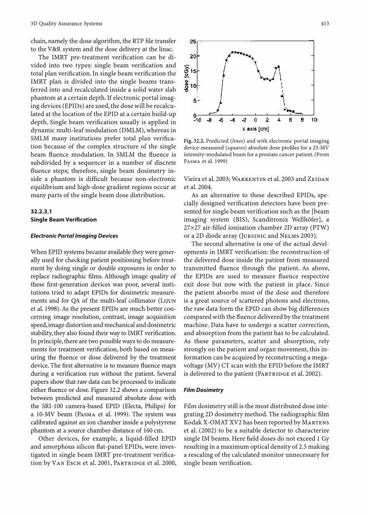
3D Quality Assurance Systems 413

chain, namely the dose algorithm, the RTP fi le transfer to the V&R system and the dose delivery at the linac.

The IMRT pre-treatment verifi cation can be di-vided into two types: single beam verifi cation and total plan verifi cation. In single beam verifi cation the IMRT plan is divided into the single beams trans-ferred into and recalculated inside a solid water slab phantom at a certain depth. If electronic portal imag-ing devices (EPIDs) are used, the dose will be recalcu-lated at the location of the EPID at a certain build-up depth. Single beam verifi cation usually is applied in dynamic multi-leaf modulation (DMLM), whereas in SMLM many institutions prefer total plan verifi ca-tion because of the complex structure of the single beam fl uence modulation. In SMLM the fl uence is subdivided by a sequencer in a number of discrete fl uence steps; therefore, single beam dosimetry in-side a phantom is diffi cult because non-electronic equilibrium and high-dose gradient regions occur at many parts of the single beam dose distribution.

32.2.3.1 Single Beam Verifi cation

Electronic Portal Imaging Devices

When EPID systems became available they were gener-ally used for checking patient positioning before treat-ment by doing single or double exposures in order to replace radiographic fi lms. Although image quality of these fi rst-generation devices was poor, several insti-tutions tried to adapt EPIDs for dosimetric measure-ments and for QA of the multi-leaf collimator (Lijun et al. 1998). As the present EPIDs are much better con-cerning image resolution, contrast, image acquisition speed, image distortion and mechanical and dosimetric stability, they also found their way to IMRT verifi cation. In principle, there are two possible ways to do measure-ments for treatment verifi cation, both based on meas-uring the fl uence or dose delivered by the treatment device. The fi rst alternative is to measure fl uence maps during a verifi cation run without the patient. Several papers show that raw data can be processed to indicate either fl uence or dose. Figure 32.2 shows a comparison between predicted and measured absolute dose with the SRI-100 camera-based EPID (Electa, Philips) for a 10-MV beam (Pasma et al. 1999). The system was calibrated against an ion chamber inside a polystyrene phantom at a source chamber distance of 160 cm.

Other devices, for example, a liquid-fi lled EPID and amorphous silicon fl at-panel EPIDs, were inves-tigated in single beam IMRT pre-treatment verifi ca-tion by Van Esch et al. 2001, Partridge et al. 2000,

Vieira et al. 2003; Warkentin et al. 2003 and Zeidan et al. 2004.

As an alternative to these described EPIDs, spe-cially designed verifi cation detectors have been pre-sented for single beam verifi cation such as the [beam imaging system (BIS), Scanditronix Wellhöfer], a 27×27 air-fi lled ionisation chamber 2D array (PTW) or a 2D diode array (Jursinic and Nelms 2003).

The second alternative is one of the actual devel-opments in IMRT verifi cation: the reconstruction of the delivered dose inside the patient from measured transmitted fl uence through the patient. As above, the EPIDs are used to measure fl uence respective exit dose but now with the patient in place. Since the patient absorbs most of the dose and therefore is a great source of scattered photons and electrons, the raw data form the EPID can show big differences compared with the fl uence delivered by the treatment machine. Data have to undergo a scatter correction, and absorption from the patient has to be calculated. As these parameters, scatter and absorption, rely strongly on the patient and organ movement, this in-formation can be acquired by reconstructing a mega-voltage (MV) CT scan with the EPID before the IMRT is delivered to the patient (Partridge et al. 2002).

Film Dosimetry

Film dosimetry still is the most distributed dose inte-grating 2D dosimetry method. The radiographic fi lm Kodak X-OMAT XV2 has been reported by Martens et al. (2002) to be a suitable detector to characterize single IM beams. Here fi eld doses do not exceed 1 Gy resulting in a maximum optical density of 2.5 making a rescaling of the calculated monitor unnecessary for single beam verifi cation.

Fig. 32.2. Predicted (lines) and with electronic portal imaging device-measured (squares) absolute dose profi les for a 25-MV intensity-modulated beam for a prostate cancer patient. (From Pasma et al. 1999)

414 B. Rhein and P. Häring

In total beam verifi cation the maximum dose per fraction can be up to 2.5 Gy, especially in IMRT plans with an integrated boost exceeding the dynamic range of this radiographic fi lm; therefore, a new Kodak fi lm with extended dose range EDR2 is available with an optical density of about 1.5–1.7 at an absorbed dose of 2 Gy.

The energy-dependent response of the EDR2 and the XV2 fi lms remain within 3% as long as the fi eld size does not increase above 15×15 cm2 (Dogan et al. 2002; Esthappan et al. 2002; Olch 2002; Zhu XR et al. 2002).

With increasing fi eld size the mean energy inside the fi eld will decrease because of the higher frac-tion of scattered low-energy photons and therefore the fi lm response will increase. The 6 MV (Siemens PRIMUS) photon spectrum in water at 5 cm depth was calculated using the MC code BEAMnrc at the fi eld sizes 2×2, 10×10 and 20×20 cm2.The main dif-ference in photon fl uence is detectable between 100 and 400 keV while the ratio of the mass energy ab-sorption coeffi cients increases dramatically below 100 keV with a maximum at 60 keV (Fig. 32.3).

Fig. 32.3. a Siemens PRIMUS 6-MV photon fl uence spectra calculated with the MC code BEAMnrc at the fi eld sizes 2×2, 10×10 and 20×20 cm2 at 5 cm depth in water. b Energy-de-pendent ratio of the mass energy absorption coeffi cients fi lm to water

Fig. 32.4. Response of Kodak EDR 2 fi lm as a function of fi eld size (triangles). In comparison, the variation of the KQ val-ues for a PTW M31002 0.125-cm3 ion chamber is illustrated (dots).

b

a

The fi eld-size-dependent response of the EDR2 fi lms was examined experimentally. Optical densities were evaluated after the fi lms were exposed with 2 Gy at fi eld sizes between 2×2 and 20×20 cm2. In IMRT the fi eld segments (SMLM) are in the range between 1×1 and 10×10 cm2. In DMLM the width of the moving fi eld aperture is of the same order. If fi lm calibration conditions are defi ned near the measurement con-ditions, e.g. at 5×5cm2 in a certain phantom depth, the energy- or fi eld-size dependent EDR2 response remains within ±2% (Fig. 32.4). In comparison, the variation of the KQ values for PTW M31002 varies only 1 per mille between the fi eld size of 2×2 and 20×20 cm2. The KQ values were computed according to the IAEA dosimetry protocol TRS 398.

Bucciolini et al. (2004) and Rhein et al. (2002) published fi lm calibration methods minimizing the effect of fi eld-size dependency in fi lm dosimetry.

The above-mentioned accuracy in fi lm dosimetry is only achievable if the fi lm processing as well as fi lm scanner is included in a continuous QA procedure.

Radiochromic fi lms show nearly no energy depend-ency (Muench et al. 1991), but they have a low re-sponse and need up to 50 Gy to produce a reasonable optical density. It is advantageous that they need no fi lm processing, especially in times where more clinics go fi lmless, but on the other hand, they are very expensive.

32.2.3.2 Total Beam Verifi cation

In total beam verifi cation the complete IMRT plan is transferred from the patient CT data set into a phan-tom (hybrid phantom) and the dose is recalculated to

3D Quality Assurance Systems 415

consider the phantom geometry. Especially in SMLM mode this procedure is advantageous compared with single beam verifi cation because dosimetry can be done now inside the more or less homogeneous high-dose region of the total plan dose distribution. Since the original patient RTP fi le is used, this procedure verifi es the whole IMRT QA chain, namely the dose algorithm, the fi le transfer to the V&R system and the dose delivery at the linac.

32.2.3.3 Verifi cation Phantoms

In single beam verifi cation mainly solid water slab phantoms are used together with fi lms and/or ioni-sation chambers while in total IMRT plan verifi ca-tion increasingly more special phantoms have been developed. There are all kinds of shapes, close to a patient’s outline, cylinders or just cubic phantoms, mainly made of solid water, in use. Different phan-toms have the ability to be equipped with fi lms, ioni-sation chambers, TLDs and even with bang gel and

ferrous sulphate gel inserts (Gum et al. 2002; Low et al. 1998a; Ma CM et al. 2003; Paliwal et al. 2000; Rhein et al. 2002; Richardson et al. 2003; Tsai et al. 1998). Many of them are commercially available from various dosimetry companies.

Two fi lm phantoms and two ionisation chamber phantoms used for total IMRT plan (SMLM with a Siemens PRIMUS linac) verifi cation at the German Cancer Research Centre (DKFZ) are demonstrated below.

Figure 32.5a shows a phantom built for verifi cations in the head and neck. It is a cylindrical solid water phan-tom (diameter 20 cm, height 20 cm) that is adaptable to the stereo-tactical system. For the body region a slightly modifi ed solid water slab phantom (30×30×20 cm3) is shown in Fig. 32.5b. Both phantoms can be used to perform fi lm measurements as well as point measure-ments with a diamond detector or a small volume ion chamber along the central axis. With both phantoms it is possible to mark the coordinate system onto the fi lms with a guided needle for data correlation and evalua-tion with IMRT software described later.

Fig. 32.5. a Solid water head and neck phantom for fi lm or ion chamber dosimetry. b Solid water slab phantom for fi lm or ion chamber dosimetry in the body region. c Solid water ion chamber matrix phantom for si-multaneous measurements with up to 12 ion chambers. d Lucite cylinder phantom for dosimetry with the liquid ionisation chamber array LA48

b

a

c

d

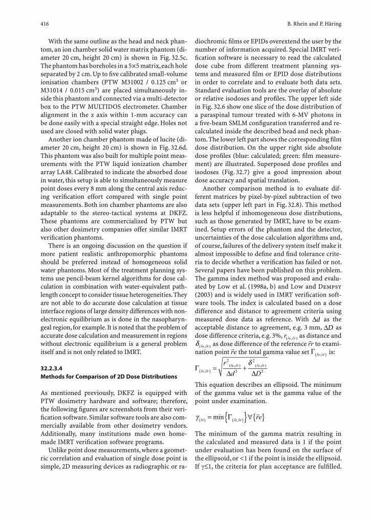
416 B. Rhein and P. Häring

diochromic fi lms or EPIDs overextend the user by the number of information acquired. Special IMRT veri-fi cation software is necessary to read the calculated dose cube from different treatment planning sys-tems and measured fi lm or EPID dose distributions in order to correlate and to evaluate both data sets. Standard evaluation tools are the overlay of absolute or relative isodoses and profi les. The upper left side in Fig. 32.6 show one slice of the dose distribution of a paraspinal tumour treated with 6-MV photons in a fi ve-beam SMLM confi guration transferred and re-calculated inside the described head and neck phan-tom. The lower left part shows the corresponding fi lm dose distribution. On the upper right side absolute dose profi les (blue: calculated; green: fi lm measure-ment) are illustrated. Superposed dose profi les and isodoses (Fig. 32.7) give a good impression about dose accuracy and spatial translation.

Another comparison method is to evaluate dif-ferent matrices by pixel-by-pixel subtraction of two data sets (upper left part in Fig. 32.8). This method is less helpful if inhomogeneous dose distributions, such as those generated by IMRT, have to be exam-ined. Setup errors of the phantom and the detector, uncertainties of the dose calculation algorithms and, of course, failures of the delivery system itself make it almost impossible to defi ne and fi nd tolerance crite-ria to decide whether a verifi cation has failed or not. Several papers have been published on this problem. The gamma index method was proposed and evalu-ated by Low et al. (1998a, b) and Low and Dempsy (2003) and is widely used in IMRT verifi cation soft-ware tools. The index is calculated based on a dose difference and distance to agreement criteria using measured dose data as reference. With ∆d as the acceptable distance to agreement, e.g. 3 mm, ∆D as dose difference criteria, e.g. 3%, r re rr( , )r r as distance and δ ( , )r rre rr as dose difference of the reference

rrr to exami-nation point

rre the total gamma value set Γ r rre rr,( ) is:

Γ∆ ∆

r r

r r r r

re rrre rr re rrrd D,

( , ) ( , )( ) = +

2

2

2

2

δ

This equation describes an ellipsoid. The minimum of the gamma value set is the gamma value of the point under examination.

γ r r rr

rr re rr re( ) ( )= { }∀{ }min ,Γ

The minimum of the gamma matrix resulting in the calculated and measured data is 1 if the point under evaluation has been found on the surface of the ellipsoid, or <1 if the point is inside the ellipsoid. If ≤1, the criteria for plan acceptance are fulfi lled.

With the same outline as the head and neck phan-tom, an ion chamber solid water matrix phantom (di-ameter 20 cm, height 20 cm) is shown in Fig. 32.5c. The phantom has boreholes in a 5×5 matrix, each hole separated by 2 cm. Up to fi ve calibrated small-volume ionisation chambers (PTW M31002 / 0.125 cm3 or M31014 / 0.015 cm3) are placed simultaneously in-side this phantom and connected via a multi-detector box to the PTW MULTIDOS electrometer. Chamber alignment in the z axis within 1-mm accuracy can be done easily with a special straight edge. Holes not used are closed with solid water plugs.

Another ion chamber phantom made of lucite (di-ameter 20 cm, height 20 cm) is shown in Fig. 32.6d. This phantom was also built for multiple point meas-urements with the PTW liquid ionization chamber array LA48. Calibrated to indicate the absorbed dose in water, this setup is able to simultaneously measure point doses every 8 mm along the central axis reduc-ing verifi cation effort compared with single point measurements. Both ion chamber phantoms are also adaptable to the stereo-tactical systems at DKFZ. These phantoms are commercialized by PTW but also other dosimetry companies offer similar IMRT verifi cation phantoms.

There is an ongoing discussion on the question if more patient realistic anthropomorphic phantoms should be preferred instead of homogeneous solid water phantoms. Most of the treatment planning sys-tems use pencil-beam kernel algorithms for dose cal-culation in combination with water-equivalent path-length concept to consider tissue heterogeneities. They are not able to do accurate dose calculation at tissue interface regions of large density differences with non-electronic equilibrium as is done in the nasopharyn-geal region, for example. It is noted that the problem of accurate dose calculation and measurement in regions without electronic equilibrium is a general problem itself and is not only related to IMRT.

32.2.3.4 Methods for Comparison of 2D Dose Distributions

As mentioned previously, DKFZ is equipped with PTW dosimetry hardware and software; therefore, the following fi gures are screenshots from their veri-fi cation software. Similar software tools are also com-mercially available from other dosimetry vendors. Additionally, many institutions made own home-made IMRT verifi cation software programs.

Unlike point dose measurements, where a geomet-ric correlation and evaluation of single dose point is simple, 2D measuring devices as radiographic or ra-

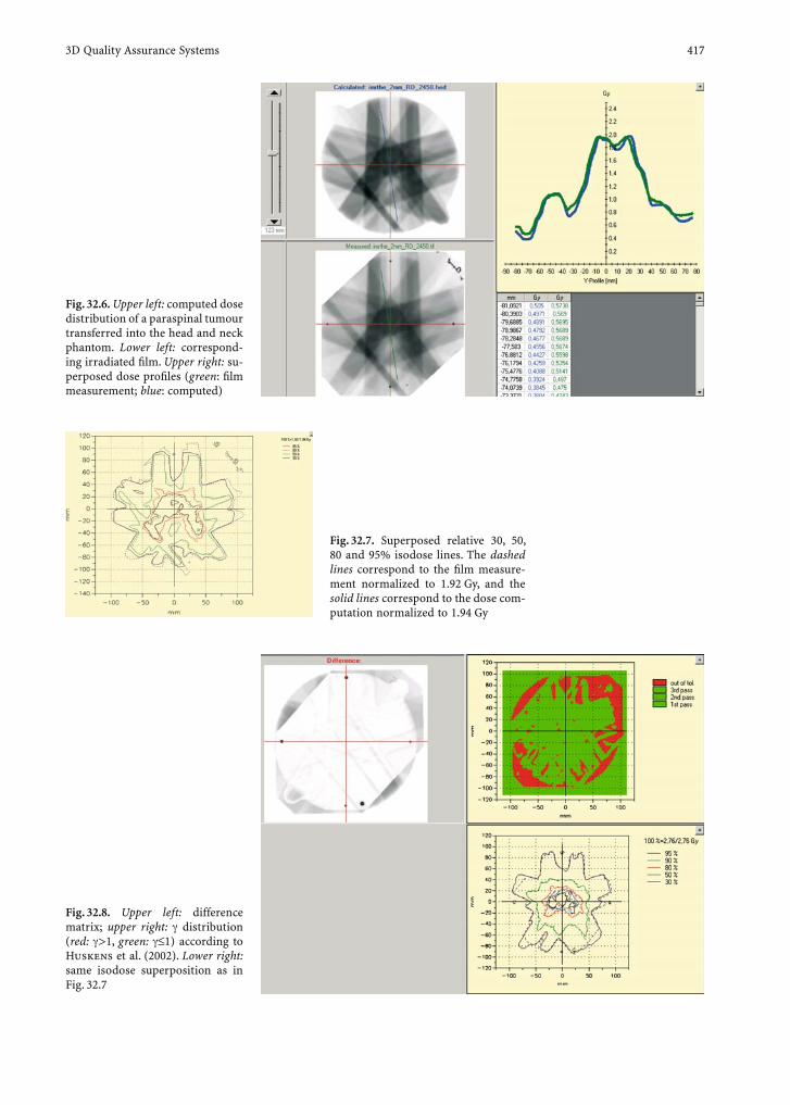
3D Quality Assurance Systems 417

Fig. 32.6. Upper left: computed dose distribution of a paraspinal tumour transferred into the head and neck phantom. Lower left: correspond-ing irradiated fi lm. Upper right: su-perposed dose profi les (green: fi lm measurement; blue: computed)

Fig. 32.7. Superposed relative 30, 50, 80 and 95% isodose lines. The dashed lines correspond to the fi lm measure-ment normalized to 1.92 Gy, and the solid lines correspond to the dose com-putation normalized to 1.94 Gy

Fig. 32.8. Upper left: difference matrix; upper right: distribution (red: >1, green: ≤1) according to Huskens et al. (2002). Lower right: same isodose superposition as in Fig. 32.7

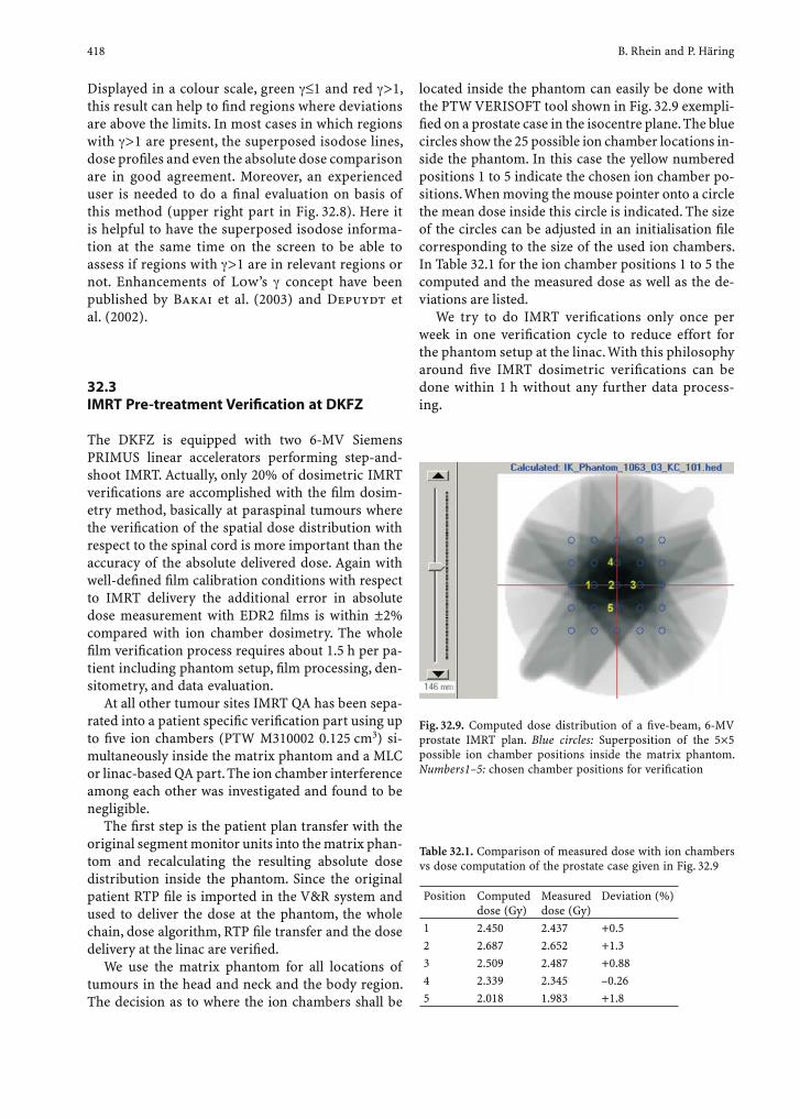
418 B. Rhein and P. Häring

Displayed in a colour scale, green ≤1 and red >1, this result can help to fi nd regions where deviations are above the limits. In most cases in which regions with >1 are present, the superposed isodose lines, dose profi les and even the absolute dose comparison are in good agreement. Moreover, an experienced user is needed to do a fi nal evaluation on basis of this method (upper right part in Fig. 32.8). Here it is helpful to have the superposed isodose informa-tion at the same time on the screen to be able to assess if regions with >1 are in relevant regions or not. Enhancements of Low’s concept have been published by Bakai et al. (2003) and Depuydt et al. (2002).

32.3 IMRT Pre-treatment Verifi cation at DKFZ

The DKFZ is equipped with two 6-MV Siemens PRIMUS linear accelerators performing step-and-shoot IMRT. Actually, only 20% of dosimetric IMRT verifi cations are accomplished with the fi lm dosim-etry method, basically at paraspinal tumours where the verifi cation of the spatial dose distribution with respect to the spinal cord is more important than the accuracy of the absolute delivered dose. Again with well-defi ned fi lm calibration conditions with respect to IMRT delivery the additional error in absolute dose measurement with EDR2 fi lms is within ±2% compared with ion chamber dosimetry. The whole fi lm verifi cation process requires about 1.5 h per pa-tient including phantom setup, fi lm processing, den-sitometry, and data evaluation.

At all other tumour sites IMRT QA has been sepa-rated into a patient specifi c verifi cation part using up to fi ve ion chambers (PTW M310002 0.125 cm3) si-multaneously inside the matrix phantom and a MLC or linac-based QA part. The ion chamber interference among each other was investigated and found to be negligible.

The fi rst step is the patient plan transfer with the original segment monitor units into the matrix phan-tom and recalculating the resulting absolute dose distribution inside the phantom. Since the original patient RTP fi le is imported in the V&R system and used to deliver the dose at the phantom, the whole chain, dose algorithm, RTP fi le transfer and the dose delivery at the linac are verifi ed.

We use the matrix phantom for all locations of tumours in the head and neck and the body region. The decision as to where the ion chambers shall be

located inside the phantom can easily be done with the PTW VERISOFT tool shown in Fig. 32.9 exempli-fi ed on a prostate case in the isocentre plane. The blue circles show the 25 possible ion chamber locations in-side the phantom. In this case the yellow numbered positions 1 to 5 indicate the chosen ion chamber po-sitions. When moving the mouse pointer onto a circle the mean dose inside this circle is indicated. The size of the circles can be adjusted in an initialisation fi le corresponding to the size of the used ion chambers. In Table 32.1 for the ion chamber positions 1 to 5 the computed and the measured dose as well as the de-viations are listed.

We try to do IMRT verifi cations only once per week in one verifi cation cycle to reduce effort for the phantom setup at the linac. With this philosophy around fi ve IMRT dosimetric verifi cations can be done within 1 h without any further data process-ing.

Fig. 32.9. Computed dose distribution of a fi ve-beam, 6-MV prostate IMRT plan. Blue circles: Superposition of the 5×5 possible ion chamber positions inside the matrix phantom. Numbers1–5: chosen chamber positions for verifi cation

Table 32.1. Comparison of measured dose with ion chambers vs dose computation of the prostate case given in Fig. 32.9

Position Computed dose (Gy)

Measured dose (Gy)

Deviation (%)

1 2.450 2.437 +0.52 2.687 2.652 +1.33 2.509 2.487 +0.884 2.339 2.345 –0.265 2.018 1.983 +1.8

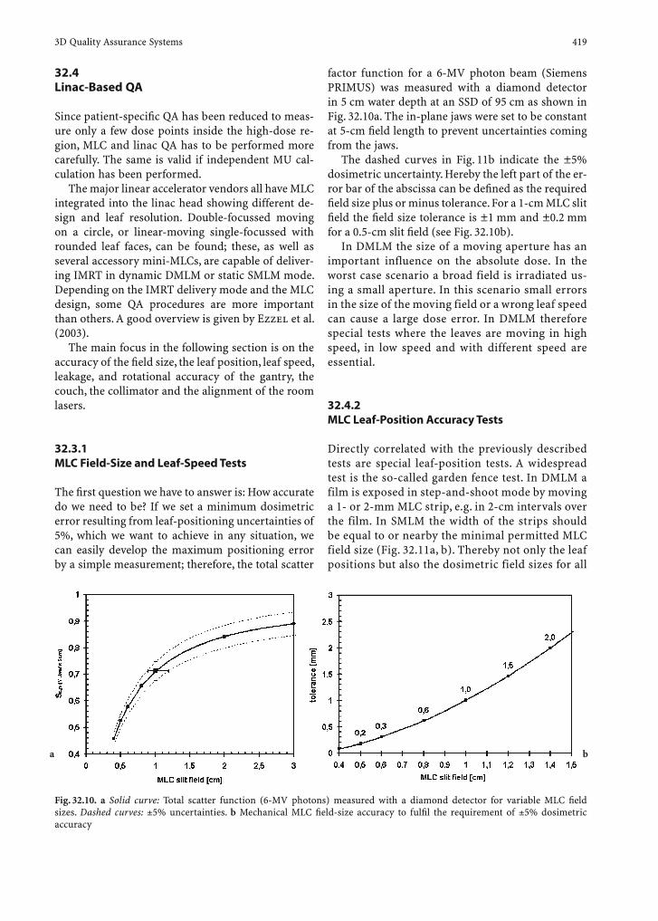
3D Quality Assurance Systems 419

32.4 Linac-Based QA

Since patient-specifi c QA has been reduced to meas-ure only a few dose points inside the high-dose re-gion, MLC and linac QA has to be performed more carefully. The same is valid if independent MU cal-culation has been performed.

The major linear accelerator vendors all have MLC integrated into the linac head showing different de-sign and leaf resolution. Double-focussed moving on a circle, or linear-moving single-focussed with rounded leaf faces, can be found; these, as well as several accessory mini-MLCs, are capable of deliver-ing IMRT in dynamic DMLM or static SMLM mode. Depending on the IMRT delivery mode and the MLC design, some QA procedures are more important than others. A good overview is given by Ezzel et al. (2003).

The main focus in the following section is on the accuracy of the fi eld size, the leaf position, leaf speed, leakage, and rotational accuracy of the gantry, the couch, the collimator and the alignment of the room lasers.

32.3.1 MLC Field-Size and Leaf-Speed Tests

The fi rst question we have to answer is: How accurate do we need to be? If we set a minimum dosimetric error resulting from leaf-positioning uncertainties of 5%, which we want to achieve in any situation, we can easily develop the maximum positioning error by a simple measurement; therefore, the total scatter

factor function for a 6-MV photon beam (Siemens PRIMUS) was measured with a diamond detector in 5 cm water depth at an SSD of 95 cm as shown in Fig. 32.10a. The in-plane jaws were set to be constant at 5-cm fi eld length to prevent uncertainties coming from the jaws.

The dashed curves in Fig. 11b indicate the ±5% dosimetric uncertainty. Hereby the left part of the er-ror bar of the abscissa can be defi ned as the required fi eld size plus or minus tolerance. For a 1-cm MLC slit fi eld the fi eld size tolerance is ±1 mm and ±0.2 mm for a 0.5-cm slit fi eld (see Fig. 32.10b).

In DMLM the size of a moving aperture has an important influence on the absolute dose. In the worst case scenario a broad field is irradiated us-ing a small aperture. In this scenario small errors in the size of the moving field or a wrong leaf speed can cause a large dose error. In DMLM therefore special tests where the leaves are moving in high speed, in low speed and with different speed are essential.

32.4.2 MLC Leaf-Position Accuracy Tests

Directly correlated with the previously described tests are special leaf-position tests. A widespread test is the so-called garden fence test. In DMLM a film is exposed in step-and-shoot mode by moving a 1- or 2-mm MLC strip, e.g. in 2-cm intervals over the film. In SMLM the width of the strips should be equal to or nearby the minimal permitted MLC field size (Fig. 32.11a, b). Thereby not only the leaf positions but also the dosimetric field sizes for all

Fig. 32.10. a Solid curve: Total scatter function (6-MV photons) measured with a diamond detector for variable MLC fi eld sizes. Dashed curves: ±5% uncertainties. b Mechanical MLC fi eld-size accuracy to fulfi l the requirement of ±5% dosimetric accuracy

ba

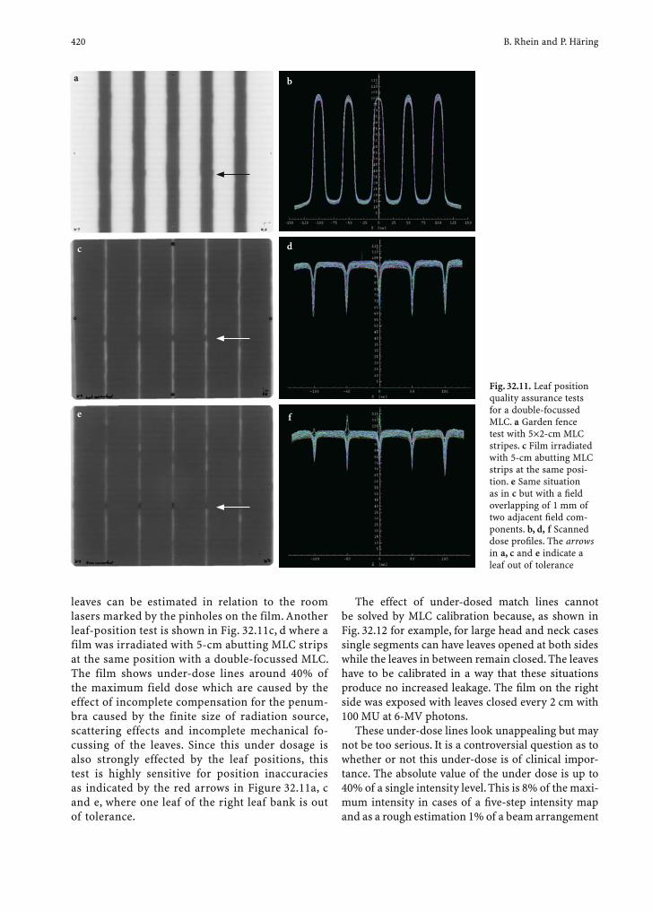
420 B. Rhein and P. Häring

leaves can be estimated in relation to the room lasers marked by the pinholes on the film. Another leaf-position test is shown in Fig. 32.11c, d where a film was irradiated with 5-cm abutting MLC strips at the same position with a double-focussed MLC. The film shows under-dose lines around 40% of the maximum field dose which are caused by the effect of incomplete compensation for the penum-bra caused by the finite size of radiation source, scattering effects and incomplete mechanical fo-cussing of the leaves. Since this under dosage is also strongly effected by the leaf positions, this test is highly sensitive for position inaccuracies as indicated by the red arrows in Figure 32.11a, c and e, where one leaf of the right leaf bank is out of tolerance.

The effect of under-dosed match lines cannot be solved by MLC calibration because, as shown in Fig. 32.12 for example, for large head and neck cases single segments can have leaves opened at both sides while the leaves in between remain closed. The leaves have to be calibrated in a way that these situations produce no increased leakage. The fi lm on the right side was exposed with leaves closed every 2 cm with 100 MU at 6-MV photons.

These under-dose lines look unappealing but may not be too serious. It is a controversial question as to whether or not this under-dose is of clinical impor-tance. The absolute value of the under dose is up to 40% of a single intensity level. This is 8% of the maxi-mum intensity in cases of a fi ve-step intensity map and as a rough estimation 1% of a beam arrangement

Fig. 32.11. Leaf position quality assurance tests for a double-focussed MLC. a Garden fence test with 5×2-cm MLC stripes. c Film irradiated with 5-cm abutting MLC strips at the same posi-tion. e Same situation as in c but with a fi eld overlapping of 1 mm of two adjacent fi eld com-ponents. b, d, f Scanned dose profi les. The arrows in a, c and e indicate a leaf out of tolerance

a

c

e

b

d

f

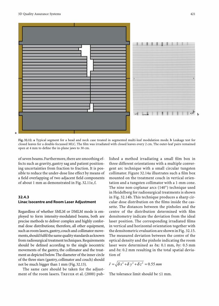
3D Quality Assurance Systems 421

of seven beams. Furthermore, there are smoothing ef-fects such as gravity, gantry sag and patient position-ing uncertainties from fraction to fraction. It is pos-sible to reduce the under-dose line effect by means of a fi eld overlapping of two adjacent fi eld components of about 1 mm as demonstrated in Fig. 32.11e, f.

32.4.3 Linac Isocentre and Room Laser Adjustment

Regardless of whether SMLM or DMLM mode is em-ployed to form intensity-modulated beams, both are precise methods to deliver complex and highly confor-mal dose distributions; therefore, all other equipment, such as room lasers, gantry, couch and collimator move-ments, should fulfi l the same quality standards as known from radiosurgical treatment techniques. Requirements should be defi ned according to the single isocentric movements of the gantry, the collimator and the treat-ment as depicted below. The diameter of the inner circle of the three stars (gantry, collimator and couch) should not be much bigger than 1 mm (Fig. 32.13).

The same care should be taken for the adjust-ment of the room lasers. Treuer et al. (2000) pub-

lished a method irradiating a small fi lm box in three different orientations with a multiple conver-gent arc technique with a small circular tungsten collimator. Figure 32.14a illustrates such a fi lm box mounted on the treatment couch in vertical orien-tation and a tungsten collimator with a 1-mm cone. The nine non-coplanar arcs (140°) technique used in Heidelberg for radiosurgical treatments is shown in Fig. 32.14b. This technique produces a sharp cir-cular dose distribution on the fi lms inside the cas-sette. The distances between the pinholes and the centre of the distribution determined with fi lm densitometry indicate the deviation from the ideal laser position. The corresponding irradiated fi lms in vertical and horizontal orientation together with the densitometric evaluation are shown in Fig. 32.15. The measured deviation between the centre of the optical density and the pinhole indicating the room laser were determined as x: 0.1 mm, y: 0.5 mm and z: 0.2 mm resulting in the total spatial devia-tion of

rr x y z mm= + + =δ δ δ2 2 2 0 55.

The tolerance limit should be ≤1 mm.

Fig. 32.12. a Typical segment for a head and neck case treated in segmented multi-leaf modulation mode. b Leakage test for closed leaves for a double-focussed MLC. The fi lm was irradiated with closed leaves every 2 cm. The outer-leaf pairs remained open at 4 mm to defi ne the in-plane jaws to 30 cm.

b

a

422 B. Rhein and P. Häring

Fig. 32.14. a Film box used for room laser quality assurance mounted in vertical orientation at the treatment couch. b Nine non-coplanar arc technique for radiosurgical treatments with circular tungsten collimators

Fig. 32.13. Isocentric star shots of a the gantry, b the treatment couch and c the collimator. The fi lms were exposed with fi eld width of 4 mm.

Fig. 32.15a,b. Quality assurance of room laser adjustment. a Extracted dose profi les through the pinhole along the stereotactic x,z coordinates. The fi lm box was mounted in horizontal orientation. b Extracted dose profi les through the pinhole along the stereotactic y,z coordinates. The fi lmbox was mounted in vertical orientation.

ba c

ba

a b

3D Quality Assurance Systems 423

References

Bakai A, Alber M, Nüsslin F (2003) A revision of the -evalua-tion concept for the comparison of dose distributions. Phys Med Biol 48:3543–3553

Bucciolini M, Buonamici FB, Casati M (2004) Verifi cation of IMRT fi elds by fi lm dosimetry. Med Phys 31:161–168

Depuydt T, Van Esch A, Huyskens DP (2002) A quantitative evaluation of IMRT dose distributions: refi nement and clinical assessment of the gamma evaluation. Radiother Oncol 62:309–319

Dogan N, Leybovich LB, Sehti A (2002) Comparative evaluation of Kodak EDR2 and XV2 fi lms for verifi cation of intensity modulated radiation therapy. Phys Med Biol 47:4121–4130

Esthappan J, Mustic S, Harms WB, Dempsey JF, Low DA (2002) Dosimetry of therapeutic photon beams using an extended dose range fi lm. Med Phys 29:2438–2445

Ezzel GA, Galvin JM, Low DA, Palta JR, Rosen I, Sharpe MB, Xia P, Xiao Y, Xing L, Yu C (2003) Guidance document on delivery, treatment planning, and clinical implementation of IMRT: report of the IMRT subcommittee of the AAPM radiation therapy committee. Med Phys 30:2089–2115

Gum F, Scherer J, Bogner L, Rhein B, Bock M (2002) Verifi -cation of IMRT treatment plans using an inhomogeneous anthropomorphic Fricke gel phantom and 3D magnetic resonance dosimetry. Phys Med Biol 47:N67–N77

Jursinic PA, Nelms BE (2003) A 2-D diode array and analysis software for verifi cation of intensity modulated radiation therapy delivery. Med Phys 30:870–879

Laub WU, Wong T (2003) The volume effect of detectors in the dosimetry of small fi elds used in IMRT. Med Phys 30:341–347

Lijun M, Boyer AL, Findley DO, Geis PB, Mok E (1998) Appli-cation of a video-optical beam imaging system for quality assurance of medical accelerators. Phys Med Biol 43:3649–3659

Low DA, Dempsy JF (2003) Evaluation of the gamma dose dis-tribution comparison method. Med Phys 30:2455–2464

Low DA, Gerber RL, Mutic S, Purdy JA (1998a) Phantoms for IMRT dose distribution measurement and treatment veri-fi cation. Int J Radiat Oncol Biol Phys 40:1231–1235

Low DA, Harms WB, Mutic S, Purdy JA (1998b) A technique for the quantitative evaluation of dose distributions. Med Phys 25:656–661

Ma CM, Pawlicki T, Jiang SB, Li JS, Deng J, Mok E, Kapur A, Xing L, Ma L, Boyer AL (2000) Monte Carlo verifi cation of IMRT dose distributions from a commercial treatment planning optimization system. Phys Med Biol 45:2483–2495

Ma CM, Jiang, SB, Pawlicki T, Chen Y, Li JS, Deng J, Boyer AL (2003) A quality assurance phantom for IMRT dose verifi -cation. Phys Med Biol 48:561–572

Martens C, De Wagter C, De Neve W (2002) The value of radi-ographic fi lm for the characterization of intensity-modu-lated beams. Phys Med Biol 47:2221–2234

Muench PJ, Meigooni AS, Nath R, McLaughlin WL (1991) Photon energy dependence of the sensitivity of radiochro-mic fi lm and comparison with silver halide fi lm and LIF TLDs used for brachtherapy dosimetry. Med Phys 4:769–775

Olch AJ (2002) Dosimetric performance of an enhanced dose

range radiographic fi lm for intensity-modulated radiation therapy quality assurance. Med Phys 29 2159–2168

Paliwal B, Tomé W, Richardson S, Mackie TR (2000) A spiral phantom for IMRT and tomotherapy treatment delivery verifi cation. Med Phys 27:2503–2507

Partridge M, Saymond-Taylor JRN, Evans PM (2000) IMRT verifi cation with a camera based electronic portal imaging system. Phys Med Biol 45:183–196

Partridge M, Ebert M, Hesse BM (2002) IMRT verifi cation by three-dimensional dose reconstruction from portal beam measurements. Med Phys 29:1847–1858

Pasma KL, Dirkx MLP, Kroonvijk M, Visser AG, Heijmen BJM (1999) Dosimetric verifi cation of intensity modu-lated beams produced with dynamic multileaf collima-tion using an electronic portal imaging device. Med Phys 26:2373–2378

Rhein B, Häring P, Debus J, Schlegel W (2002) Dosimetrische Verfi kation von IMRT- Gesamtplänen am Deutschen Krebs-forschungszentrum Heidelberg. Z Med Phys 12:122–132

Richardson SL, Tomé WA, Orton NP, McNutt TR, Paliwal BR (2003) IMRT delivery verifi cation using a spiral phantom. Med Phys 30:2553–2558

Treuer H, Hoevels M, Luyken K, Gierich A, Kocher M, Müller R-P, Sturm V (2000) On isocentre adjustment and quality con-trol in linear accelerator based radiosurgery with circular collimators and room lasers. Phys Med Biol:45:2331–2342

Tsai JS, Wazer DE, Ling MN, Wu JK, Fargundes M, DiPetrillo T, Kramer B, Koistinen M, Engler MJ (1998) Dosimetric verifi -cation of the dynamic intensity modulated radiation of 92 patients. Int J Radiat Oncol Biol Phys 40:1213–1230

Van Esch A, Vanstraelen B, Verstraete J, Kutcher G, Huyskens D (2001) Pre-treatment dosimetric verifi cation by means of a liquid fi lled electronic portal imaging device during dynamic delivery of intensity modulated treatment fi elds. Radiother Oncol 60:181–190

Vieira SC, Dirkx MLP, Pasma KL, Heijmen BJM (2003) Dosi-metric verifi cation of X-ray fi elds with steep dose gradients using an electronic portal imaging device. Phys Med Biol 48:157–166

Warkentin B, Steciv S, Rathee S, Fallone BG (2003) Dosimet-ric IMRT verifi cation with a fl at-panel EPID. Med Phys 30:3143–3155

Xing L, Chen J, Luxton G, Li GJ, Boyer AL (2000) Monitor unit calculation for an intensity modulated photon fi eld by a simple scatter summation algorithm. Phys Med Biol 45:1–7

Yang Y, Xing L, Li JG, Palta J, Chen Y, Luxton G, Boyer A (2003) Independent dosimetric calculation with inclusion of head scatter and MLC transmission for IMRT. Med Phys 30:2937–2947

Zeidan OA, Li JG, Ranade M, Stell AM, Dempsey JF (2004) Verifi cation of step and shoot IMRT delivery using a fast video-based electronical portal imaging device. Med Phys 31:463–476

Zhu J, Yin FF, Kim JH (2003) Point dose verifi cation for inten-sity modulated radiosurgery using Clarkson’s method. Med Phys 30:2218–2221

Zhu XR, Jursinic PA, Grimm DF, Lopez F, Rownd JJ, Gillin MT(2002) Evaluation of Kodak EDR2 fi lm for dose verifi -cation of intensity modulated radiation therapy delivered by a static multileaf collimator. Med Phys 29:1687–1692

Quality Management in Radiotherapy 425

33 Quality Management in Radiotherapy

Guenther H. Hartmann

G. H. Hartmann, PhDDepartment of Medical Physics in Radiotherapy, Deutsches Krebsforschungszentrum, Im Neuenheimer Feld 280, 69120 Heidelberg, Germany

CONTENTS

33.1 Introduction 42533.2 Objectives of a QMS in Radiotherapy 42633.2.1 Maintaining the Required Accuracy 42633.2.2 Minimizing the Risk of Errors and Accidents 42733.2.3 Further Arguments 42833.3 Comprehensive Quality Management Program 42933.3.1 Introduction 42933.3.2 QM Project Team 43033.3.3 Structure of the Quality System 43033.3.4 Policy 43033.3.5 Responsibilities 43133.3.6 Requirements for Quality 43133.3.7 Quality Manual 43233.3.8 The Treatment Planning Process as a Guide to Structure the Quality Manual 43233.3.9 Implementation 43233.3.10 Quality Audit and Continuous Quality Improvement 43333.3.10.1 Defi nition 43333.3.10.2 Practical Quality Audit Modalities 43433.4 Quality System for Radiotherapy Equipment 43433.4.1 General 43433.4.2 Terminology 43533.4.3 QA Protocol 43533.4.3.1 Structure of Equipment-Specifi c QA Program 43533.4.3.2 Clinical Needs Assessment and Initial Specifi cation for Purchase 43533.4.3.3 Acceptance Tests 43633.4.4 Commissioning 43733.4.4.1 Acquisition of Photon Beam Data 43833.4.5 Periodic Tests 44133.4.5.1 Test Program 44134,4.5.2 Uncertainties, Tolerances, and Action Levels 44234.4.5.3 Periodic Tests for Linear Accelerators 44234.4.5.4 Periodic Tests for TPS 44433.5 Clinical Aspects of QA 44433.5.1 New Patient Planning Conference 44433.5.2 Chart Review 44533.5.3 Film/Image Review 446 References 446

33.1 Introduction

It is anticipated that radiotherapy will have an in-creasing role in treating cancer patients; however, all recent developments in radiotherapy technology and the improved performance of modern equip-ment cannot be fully exploited unless a high degree of accuracy and reliability in dose delivery is reached. To meet this requirement, sustained efforts have to be applied to all areas of the radiotherapy process.

It is a characteristic feature of modern radiother-apy that this process is a multi-disciplinary process involving complex equipment and procedures for the delivery of treatment; therefore, it is extremely important that (a) the radiation therapist cooperate with specialists in the various disciplines in a close and effective manner, and (b) the various procedures (related to the patient and that related to the techni-cal aspects of radiotherapy) be subjected to careful quality control. The establishment and use of a com-prehensive quality system (QS) is an adequate mea-sure to meet all these requirements.

A number of organizations, such as WHO, AAPM, ESTRO, and IPEM, and also other publications have given background discussion and recommendations on the structure and management of a QS in radio-therapy (American Association of Physics in Medicine 1994a; Mayles et al. 1999; Leer et al. 1995, 1998; McKenzie et al. 2000; Thwaites et al. 1995; Van Dyk et al. 1993; World Health Organization 1988). Historically, actions summarized under the term “quality assurance” (QA) has long been carried out in many areas of radiotherapy, particularly in the more readily defi ned physical and technical aspects of equipment, dosimetry, and treatment delivery. Presently, however, it is generally appreciated that the concept of quality in radiotherapy is broader than a restricted defi nition of technical maintenance and quality control of equipment and treatment delivery, and instead that it should encompass a comprehensive approach to all activities in the radiotherapy depart-ment; thus, it has clinical, physical, and administrative

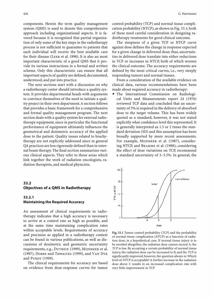
426 G. Hartmann

components. Herein the term quality management system (QMS) is used to denote this comprehensive approach including organizational aspects. It is fa-vored because it is recognized that partial organiza-tion of only some of the key steps in the radiotherapy process is not suffi cient to guarantee to patients that each individual will receive the best available care for their disease (Leer et al. 1998). It is also an most important characteristic of a good QMS that it pro-vide its various instructions in a formal and written scheme. Only this characteristic can ensure that all important aspects of quality are defi ned, documented, understood, and put into practice.

The next sections start with a discussion on why a radiotherapy center should introduce a quality sys-tem. It provides departmental heads with arguments to convince themselves of the need to initiate a qual-ity project in their own department. A section follows that provides a basic framework for a comprehensive and formal quality management program. The next section deals with a quality system for external radio-therapy equipment, since in particular the functional performance of equipment ultimately infl uences the geometrical and dosimetric accuracy of the applied dose to the patient. Quality issues related to brachy-therapy are not explicitly addressed since in general QA practices are less rigorously defi ned than in exter-nal beam therapy. The fi nal section summarizes vari-ous clinical aspects. They refer to those areas which link together the work of radiation oncologists, ra-diation therapists, and medical physicists.

33.2 Objectives of a QMS in Radiotherapy

33.2.1 Maintaining the Required Accuracy

An assessment of clinical requirements in radio-therapy indicates that a high accuracy is necessary to arrive at a control rate as high as possible, and at the same time maintaining complication rates within acceptable levels. Requirements of accuracy and precision as applied in a radiotherapy context can be found in various publications, as well as dis-cussions of dosimetric and geometric uncertainty requirements, e.g., Dutreix (1999), Mijnheer et al. (1987), Dobbs and Thwaites (1999), and Van Dyk and Purdy (1999).

The clinical requirements for accuracy are based on evidence from dose-response curves for tumor

control probability (TCP) and normal tissue compli-cation probability (NTCP), as shown in Fig. 33.1; both of these need careful consideration in designing ra-diotherapy treatments for good clinical outcome.

The steepness of a given TCP or NTCP curve against dose defi nes the change in response expected for a given change in delivered dose; thus, uncertain-ties in delivered dose translate into either reductions in TCP or increases in NTCP, both of which worsen the clinical outcome. The accuracy requirements are defi ned by the most critical curves, i.e., very steeply responding tumors and normal tissues.

From a consideration of the available evidence on clinical data, various recommendations have been made about required accuracy in radiotherapy:• The International Commission on Radiologi-

cal Units and Measurements report 24 (1976) reviewed TCP data and concluded that an uncer-tainty of 5% is required in the delivery of absorbed dose to the target volume. This has been widely quoted as a standard; however, it was not stated explicitly what confi dence level this represented. It is generally interpreted as 1.5 or 2 times the stan-dard deviation (SD) and this assumption has been broadly supported by more recent assessments. For example, Mijnheer et al. (1987), consider-ing NTCP, and Brahme et al. (1988), considering the effect of dose variations on TCP, recommend a standard uncertainty of 3–3.5%. In general, the

Fig. 33.1 Tumor control probability (TCP) and the probability of normal tissue complication (NTCP) as a function of radia-tion dose, in a hypothetical case. If normal tissue injury is to be avoided altogether, the radiation dose cannot exceed A; the TCP is low. By accepting a certain probability of normal tissue injury, the radiation dose can be increased to B, and the TCP is signifi cantly improved; however, the question always is: Which level of NTCP is acceptable? A further increase in the radiation dose above C results in an increased complication rate with very little improvement in TCP

Quality Management in Radiotherapy 427

smallest of these numbers might be applicable to the simplest situations, with the minimum number of parameters involved, whereas the larger fi gure (3.5%) is more realistic for practical clinical radio-therapy when more complex treatment situations and patient factors are considered.

• Geometric uncertainty relative to target volumes or organs at risk also lead to dose problems, either underdosing of the required volume (decreas-ing the TCP) or overdosing of nearby structures (increasing the NTCP). Consideration of these effects has led to recommendations on spatial uncertainty of between 5 and 10 mm (at the 95% confi dence level). The fi gure of 5 mm is generally applied to the overall equipment-related mechani-cal/geometric problems, whereas larger fi gures (typically 8 or 10 mm) are used to indicate overall spatial accuracy including representative contri-butions for problems related to the patient and to clinical setup. The latter factors obviously depend on the site involved, the method of immobiliza-tion, and the treatment techniques employed.

Thus, the recommended accuracy on dose deliv-ery is generally 5–7% on the 95% confi dence level, depending on the factors intended to be included. On spatial accuracy, fi gures of 5–10 mm (95% confi dence level) are usually given, depending on the factors intended to be included. These are general require-ments for routine clinical practice. In some specifi c applications, such as stereotactic radiotherapy, IMRT, or radiotherapy with ion beams, better accuracy might be demanded which consequently has an im-pact on increased QA efforts.

These recommendations are for the end point of the radiotherapy process, i.e., for the entire treatment as delivered to the patient; therefore, on each of the steps that contribute to the fi nal accuracy correspond-ingly smaller values are required, such that when all are combined the overall accuracy is met. The aim of a QMS program is to maintain each step within an ac-ceptable tolerance; therefore, if a more complex treat-ment technique, more stages, sub-stages, or other pa-rameters and factors are involved, a correspondingly more complex QMS is required.

33.2.2 Minimizing the Risk of Errors and Accidents

Human error will always occur in any organization and any activity. In radiotherapy, there is the poten-tial failure to control the initial disease which, when

it is malignant, is eventually lethal to the patient or there is the risk to normal tissue from increased ex-posure to radiation; thus, in radiotherapy an accident or a misadministration is signifi cant, if it results in either an underdose or an overdose. It is another im-portant objective of a QMS to minimize the number of occurrences of “errors” and to identify them at the earliest possible opportunity, thereby minimizing their consequences.

When is a difference between prescribed and de-livered dose considered to be at the level of an ac-cident or a misadministration in external beam ra-diotherapy?• From the general aim for an accuracy approach-

ing 5% (95% confi dence level), about twice this seems to be an accepted limit for the defi nition of an accidental exposure, i.e., a 10% difference.

• For example, in several jurisdictions, levels are set for reporting to regulatory authorities, if equip-ment malfunctions are discovered which would lead to a 10% difference in a whole treatment or 20% in a single fraction.

• In addition, from clinical observations of outcome and of normal tissue reactions, there is good evi-dence that differences of 10% in dose are detect-able in normal clinical practice. Additional dose applied incidentally outside the proposed target volume may lead to increased complications.

Review of AccidentsThe International Atomic Energy Agency (2000a) has recently analyzed a series of accidental exposures in radiotherapy to draw lessons in meth-ods for prevention of such occurrences. A classifi ca-tion of causes for accidents in external beam therapy, as shown in Tables 33.1 and 33.2, was given. For more details the reader is referred to the original IAEA publication.

Problems with EquipmentTable 33.1 refers to accidents related to problems with equipment, such as calibration of the beam output. Such events involve all patients treated with the beam until the problem is discovered. The most important events were those resulting in an error in the determi-nation of dose rate, and therefore wrong irradiation times for patients treated under these conditions. In the three worst cases, 115, 207, and 426 patients were involved, with dose deviations of up to 60% and many deaths. In addition, there were two major accidents related to maintenance of accelerators, one of them involving 27 patients (several of whom died as a di-rect result of radiation exposure).

428 G. Hartmann

Table 33.1 Events related to problems with equipment

Equipment Step at which the event occurred No. of eventsRadiation measurement system (including ionization chambers and electrometer)

Calibration of reference system 1Intercomparison with secondary system 1Routine use 3

Treatment machine Commissioning (acceptance) 6Calibration (annual) 3Constancy check (daily, weekly) 1Malfunction of machine 7Incorrect use 6

Simulator Malfunction 3Treatment planning system Commissioning and input of basic data 5

Routine use 6

Table 33.2 Events involving individual patients

Process Step at which the event occurred No. of eventsPrescription Miscommunication of prescription 6

Error in use of images 3Treatment planning Documentation 1

Calculation of treatment time or monitor units 3Incorrect use of treatment planning system 4

Execution of treatment Patient identifi cation 2Documentation of patient setup 9Incorrect operation of treatment machine 2Final review at completion of treatment 1

Events Involving Individual PatientsSome of the accidents reviewed occurred due to differ-ent conventions for the incorporation of different di-agnostic imaging modalities that are used in treatment planning, including those from simulators, computer tomography scanners, nuclear medicine, ultrasound, etc. Also, accidents were caused by incomplete or inac-curate documentation of patient charts for all aspects of treatment planning, including isodose curves, use of wedges, special blocking and placement, and orienta-tion of beams, since these factors are used to calculate beam-on times for all fi elds. There were cases of treat-ments to the wrong person or the wrong anatomical site, and of incorrect tumor dose and overdose to nor-mal tissues because of ineffective institutional protocol for patient identifi cation, such as a photograph of the patient, unique patient hospital number, ID bracelet, and verbal confi rmation of patient identifi cation.

These incidents are representative of typical causes. Recording, categorizing, and analyzing differ-ences in delivered and prescribed doses in radiother-apy can be carried out at many levels. The above lists give one example for the relatively small number of events reported, where large differences are involved, i.e., misadministrations.

Other evaluations have been reported from the results of in vivo dosimetry programs or other au-dits of radiotherapy practice, where smaller devia-tions, or “near misses,” have been analyzed. Similar lists of causes with similar relative frequencies have been observed. In any wide-ranging analysis of such events, at whatever level, a number of general obser-vations can be made:1. Errors may occur at any stage of the process and

by every staff group involved. Particularly criti-cal areas are interfaces between staff groups, or between processes, where information is passed across the interface.

2. Most of the immediate causes of accidental expo-sure are also related to the lack of an adequate QS program or a failure in its application.

33.2.3 Further Arguments

Sometimes the implementation of a QMS is criticized of imposing too much additional bureaucratic effort that is not really helpful. Leer et al. (28) have given

Quality Management in Radiotherapy 429

further arguments for the practical advantage of a QMS.

Continuing Quality ImprovementA QMS provides the framework for implementing the organizational structure, responsibilities, proce-dures, and resources. It must be formal, however, at the same time it must be fl exible. In particular, it must allow changes to be incorporated. If such changes are based on a systematic mechanism, such as regular audits and assessments as part of the QMS, a quality system has the potential to ensure continuing quality improvement.

Increase of Effi ciencyA QMS provides a tool for a good control of all docu-ments involved in the process of radiotherapy. The feature of allowing documents to be traced is the base to determine any discrepancy between aims and ac-tual performance. By feeding the results of the qual-ity analysis back into the process, this mechanism provides the means to increase the effi ciency.

Chance for a Cultural ChangeA QMS is most effectively introduced by involving peoples at all levels, especially the people who do the actual work. For example, when introducing a new technique it has a distinct advantage if the personnel, who are to use the new technique, offer to contribute to the written QA protocol, rather than have this task imposed on unwilling personnel. This approach may gradually result in a cultural change.

Raised Morale of PersonnelAssociated with the importance which a quality sys-tem places on training and developing personnel is the raised morale among personnel who feel, cor-rectly, that their individual needs are being given a high priority. This, of course, feeds back into the system as a benefi t. Since a quality system ensures that good communication lines are established in the organization, the misunderstandings which can arise between relatively isolated groups of personnel are less likely to occur, and there is a general awareness of being part of a well-run organization, which, itself, contributes to the raised morale.

Reduction of the Chance of LitigationAs a good QMS reduces the likelihood of errors, it will also reduce the likelihood of litigation. In a seem-ingly informed society litigation is continuing to gain prominence. So even when treatments are given ac-cording to protocol, patients increasingly use litiga-

tion, for instance when getting normal yet not an-ticipated side effects. Such litigation often demands that detailed documentation be reviewed sometimes many years after the treatment was completed. A QMS provides a method that the documentation is readily available, providing not only good defense against such litigation but also an increased cred-ibility that will help to defend the institution in the face of such litigation.

QMS as a Management ToolGood management requires good tools. A QMS pro-vides the required framework to practically accom-plish the management task; thus, good management is not left to chance.

Increase of CompetitivenessA QMS may increase the competitiveness of a radio-therapy centers. In particular, when using website in-formation increasingly offered by radiotherapy centers for comparing effi ciency, the successful implementa-tion of a QMS may be an advantage. While radiother-apy centers should aspire to a quality system for the positive benefi ts which it brings, there can be no doubt that to be surrounded by neighboring centers who run quality systems can be a motivating force.

33.3 Comprehensive Quality Management Program

33.3.1 Introduction

This section is an attempt to provide a basic frame-work for comprehensive quality management pro-gram. The document of ISO 9000 is normally referred to as a standard for a quality system. Its general prin-ciples and structures, however, must be translated into language appropriate to radiotherapy and cover-ing the complete radiotherapy process. This process can be simply summarized as shown in Fig. 33.2.

This again underlines that quality management should include not only technical aspects of the treat-ment with ionizing radiation, but also quality aspects from the patient perspective. Those aspects are pre-dominantly summarized in the last section clinical aspects.

For the purpose of QM and a QM program in ra-diotherapy, the following series of tasks should be ac-complished:

430 G. Hartmann

1. Creation of a QM project team2. Structuring the quality system3. Formulation of the department’s policy4. Description (or defi nition) of department structure5. Consideration of other requirements6. Development of a quality manual7. Implementation8. Quality audit and continuous quality improving

33.3.2 QM Project Team

In order to assure that all relevant aspects of quality, a QM project team should be formed that represents the many disciplines within radiation oncology. This committee should include a member each of the ar-eas of medicine, physics, and treatment. It is impor-tant that these members be appointed by the depart-ment chairman and that the committee be given the authority to perform its tasks. If it is possible, a short training of the members of the project team by pro-fessionals in quality management should be a start-ing activity. The committee should directly report to the head of the department on quality issues.

33.3.3 Structure of the Quality System

When introducing a quality system it is useful to dif-ferentiate between three hierarchical levels:• Level 1 refl ects (a) the defi nition of its objectives, (b)

the strategies developed to meet these objectives, and (c) the responsibilities and the structure of supervi-sion of all functions having an impact on quality the quality management. These items are summarized under the conception of “policy of the department.”

• Level 2 refers to all procedures for which a formal organization is required. In this context procedure

is a document containing information on a defi ni-tion of the scope of the procedure (what it covers and is about), of the respective responsibilities of those involved (who is responsible for doing what, who is in charge of which areas), and the outline of the practical actions to be undertaken (what is to be done).

• Finally, Level 3 work instructions explain in detail, for each separate area of practical action con-tained in a Level-2 document, how this is to be implemented at the practical level (how to do it).

33.3.4 Policy

The implementation of a QA system is successful only when it is clear what the position and the aims of the department are; therefore, the head of department has to defi ne the position and basic goals of the depart-ment. How can this be accomplished? For a starting point, there are several sources available. As an exam-ple, in Germany several associations provide a series of documents and committees as outlined in Fig. 33.3.

In the United States, the Inter-Society Council for Radiation Oncology (ISCRO), the Joint Commission on the Accreditation of Healthcare Organizations (JCAHO) the America College of Radiology (ACR), and the American College of Medical Physics (ACMP) have issued documents and requirements. More prac-tical details are outlined in the report of the American Association of Physics in Medicine Radiation Therapy Committee Task Group 40: Comprehensive QA for Radiation Oncology (1994a).

The objectives should then be laid down in a formal document, also called the policy manual, with a long-term vision on the desired development and the gen-eral consequences for budget, infrastructure, and staff-ing. Answering the following questions can be helpful to write one’s own policy manual (Leer 1998):

Fig. 33.2 Radiotherapy as a process

First presentation of the patientInformation of the patientMedical treatment planningPhysical treatment planningPreparation of auxiliary meansTreatment executionFollow-upAnalysis of relsut

Patient withcancer disease

The patient having gotten the best treatment

Radiotherapy process

Quality Management in Radiotherapy 431

• What is the expected number of cancer patients with morbidity and referral pattern?

• What is the expected number of cancer patients who are candidates for radiotherapy?

• What is the expected evolution of these numbers in the next 5–10 years?

• How is the relationship to other radiotherapy departments in the neighborhood?

• Are there agreements on the referral of patients for special treatment, e.g., stereotactic radiother-apy or hyperthermia to the department? Should such agreements be made?

• Are there agreements for the referral of patients with special types of cancer whose multidisci-plinary treatment should be centralized in the hospital, e.g., cancer in children, bone tumors, or whethersuch agreements should be made?

• Are there offi cial relations with other departments with respect to training, scientifi c work, etc.?

• Which consequences of these points are expected for the budget, infrastructure, and staffi ng?

33.3.5 Responsibilities

The next item of the policy manual is the description and/or defi nition of responsibilities. Clearly defi ned responsibility and accountability is of utmost im-portance for a comprehensive QM system. Without a clear channel of accountability, some components of the quality program will be missed or it might be assumed that someone else is responsible for a specifi c component. Ultimately, the head each depart-ment will be responsible for the overall departmental policy, for all quality matters and for the implementa-tion and maintenance of a documented quality sys-tem; however, it must be clearly stated that the quality committee acts on its own authority in his area.

Responsibility and accountability is also involved in the organizational relationship (1995); therefore, it is useful to generate an image of the structure of the department, so that each individual clearly un-derstands his or her own position in that structure, as well as that of others. In addition, the links and relationships between different individuals and staff groups should be clear. These relationships can be: (a) hierarchical, along direct management lines; (b) functional, describing an advisory relationship; or (c) operational, between members of a team work-ing on a particular project. The role and responsi-bilities of each individual should be clearly defi ned, with particular attention given to adjoining or over-lapping areas of responsibility or to areas of mul-tidisciplinary cooperation. This ensures that there are no omissions due to misinterpretation of who should carry out particular tasks. Communication between different individuals and groups should be clearly structured, with records of meetings and de-cisions.

33.3.6 Requirements for Quality

All requirements for the quality system must be de-scribed and/or defi ned in the policy manual; thus, all needs can be explicitly expressed or translated into a set of quantitatively or qualitatively stated require-ments for the characteristics of a process, procedure, or organization, in order to enable its realization and examination. Special attention must be given to in-clude obligations resulting from laws and other juris-dictional regulation. As an example, the regulations for so-called medical products for which laws have been harmonized throughout Europe have a distinct impact on the quality control of radiotherapy equip-ment.

Fig. 33.3 Network of German docu-ments steered by the Committee of Medical–Scientifi c Associations (“Arbeitsgemeinschaft der Wissenschaftlichen Medizinischen Fachgesellschaften”)

Committee ofMedical-Scientifi c

Associations (AWMF)

Association ofGerman

RadiotherapistsGerman Cancer Association

(DKG)

Topics:– general standards– interdisciplinary guidelines– quality management

German Association of Radiooncology (DEGRO)

Sub-committees:– methods– tumors / organs– quality control– co-operation with German Association of Medical Physics Guidelines

in Radiooncology

CommitteeRadiological

Oncology (ARO)

432 G. Hartmann

33.3.7 Quality Manual

The quality manual is the key document to practi-cally implement a quality program. This usually pro-gresses through four consecutive periods: a prepara-tory phase; a development phase; an implementation phase; and a consolidation phase. The steps described in the subsections above are the main components of the preparatory phase. The next following phase, the development phase, deals with describing (or defi n-ing) policy and structures, preparing procedures, and preparing work instructions. This is the point where the quality manual enters. It has a dual purpose: external and internal. Externally, to collaborators in other departments, in management and in other institutions, it helps to indicate that the department is strongly concerned with quality. Internally, it pro-vides the department with a framework for further development of quality and for improvements of ex-isting or new procedures. Basically, the quality man-ual will answer two questions for each item: What is the standard required (as a particular example: What tolerances are required on treatment unit positioning precision?), and how to meet this requirement?

Very often generally agreed upon or recommended standards are already in existence for a number of areas, particularly concerning the more well-defi ned and more easily measured technical aspects, e.g., beam calibration, beam dosimetry, mechanical sta-bility of equipment, performance of treatment plan-ning systems, patient positioning, dose delivery, etc. In other areas, agreed upon standards still need to be developed. Finally, some standards will be internal to a given department (e.g., waiting time before treat-ment) and will have to be developed locally. It is sen-sible to begin with standards set at levels which are not too strict but which can be met in the majority of cases. Setting standards which cannot be met rou-tinely is useless and kills the credibility of the qual-ity system. When deviations from these initial levels

become exceptional, then a more stringent set can be introduced as a new target to work to.

Since a complete quality manual will address a large number of procedures, experience has shown that the best way to avoid omitting any important feature of a procedure is to formalize the process of describing procedures. A possible approach is given in the next section which explicitly deals with the quality program of radiotherapy equipment.

Finally, it is recommended that everything should not be considered at once. Some aspects need to be addressed fi rst, logically those where the need for improvement has been identifi ed as urgent, whereas others can wait to be dealt with later because they are less critical. Setting up priorities is thus an important step in writing a useful quality manual.

33.3.8 The Treatment Planning Process as a Guide to Structure the Quality Manual

Treatment planning is a process that begins with pa-tient data acquisition and continues through physi-cal treatment planning, plan implementation, and treatment verifi cation. Sometimes the picture of the radiotherapy chain as shown in Fig. 33.4 is used to describe this sequence of various procedures.

The treatment planning procedures and related QA procedures as listed in Table 33.3 are taken from the report of American Association of Physics in Medicine Radiation Therapy Committee Task Group 40 (1994a). This list is a useful guide to structure the quality manual in its content.

33.3.9 Implementation

The next step to be performed is the phase of imple-mentation which covers a training phase and a vali-

Fig. 33.4 Chain of procedures involved in the radiotherapy process also referred to as the “radiotherapy chain”

Clinical evaluation

3D imaging

Treatment planning:simulation and dose calculation

Treatment planning:evaluation and selection

Dosimetry verifi cationand checks

Treatment

Follow-up evaluation

Patient positioning

Localization of target volume and organs at risk

Therapeutic decision

Quality Management in Radiotherapy 433

dation phase. At this point the following obstacle is frequently met: it is the initial belief that a quality system is too bureaucratic and rigid. Indeed, there is an element of loss of comfort which must be taken into account and the level of bureaucracy will in-crease in the department, essentially to cope with the demands on document control. It might also appear that the whole system is too stringent and inappro-priate for the size of the department and the level of activities; therefore, a subtle equilibrium needs to be found between a quality manual which is too loose and one which is too stringent. A careful design and implementation of the local quality system can contain this to a level where the benefi ts gained are recognized to be worth this cost. The best way to convince the personnel of the advantage of a quality system is to involve the personnel as soon as possible in the development of procedures and in the imple-mentation of the quality system.

From a practical point of view, the following rec-ommendations may be helpful:• Training sessions should be introduced that are

short but repeated.• They should initially be oriented towards very

practical subjects.• They should be concerned with routine daily work

before addressing wider principles.

• The aims, objectives, and rationale for the approach should be explicitly explained to the personnel at any level.

• Time for reaction and discussion, including criticism and proposals for alteration, should be allowed and provided.

• Comments should be taken into account.The objective of validation phase is to test the new

procedures, as to their appropriateness and feasibility. Advice from the users is important and must be used as a source of improvement. Any suggested improvements at this stage must be carried out rapidly. Care should be taken that any ineffi cient or unaccepted procedures not be left unchanged, as they will act as sources of general-ized de-motivation towards, and criticism of, the whole approach. The head of department must be involved and openly interested during this phase.

33.3.10 Quality Audit and Continuous Quality Improvement

33.3.10.1 Defi nition

Quality audit is a systematic and independent exami-nation to determine whether or not quality activities

Table 33.3 Treatment planning process and related quality assurance (QA) procedures. (From AAPM Radiation Therapy Committee Task Group 1994). TPS treatment planning system

Process Related QA procedure

Positioning and immobilization Port fi lms, laser alignment

Simulation Simulator QA including image and mechanical integrity

Patient data acquisition (CT, MR, manual contouring)

CT, MR, QA including image and mechanical integrity

Data transfer to treatment planning QA of entire data-transfer process, including digitizers, digital data transfer

Defi nition of target volumes Peer review (patient planning conference, chart rounds)

Aperture design Independent check of delivery, peer review

Computation of dose distribution Machine data from commissioning and QA of treatment machine; accuracy and QA of TPS

Plan evaluation Peer review of plan (chart rounds), independent check by radiation oncology physicist

Prescription Written, signed, and dated

Computation of monitor units TPS QA, independent check

Production of blocks, beam modifi ers (MLC)

QA for block cutting and compensator systems, MLCs, port fi lm review

Plan implementation Review of setup by treatment planning beam, chart review

Patient QA Treatment plan review, chart review after new or modifi ed fi eld, weekly chart review, port fi lm review, in vivo dosimetry for unusual fi elds, critical organ doses, status check, follow-up

434 G. Hartmann

and results comply with planned arrangements, and whether or not the arrangements are implemented effectively and are suitable to achieve the stated ob-jectives. Any result of non-compliance found during the process of quality audit then must be feed back into quality manual. The important point is: the qual-ity manual must be kept fl exible in such a way that it allows the possibilities of changes and improvement based on regular audits and assessments.

A detailed discussion of the structure and opera-tion of various types of quality audit is given in pa-pers by ESTRO (Leer et al. 1998), IPEM (Shaw 1996), International Atomic Energy Agency (1999), and McKenzie et al. (2000).

Parameters of quality audits are given below. Quality audits:• Are performed by personnel not directly respon-

sible for the areas being audited, preferably in cooperative discussion with the responsible per-sonnel.

• Evaluate the need for improvement or corrective action.

• Should not be confused with a surveillance or inspection.

• Can be conducted for internal or external purposes.• Can be applied at any level of a QA program.• Must be against pre-determined standards, linked

to those that the QA program is trying to achieve.• Should require action if those standards are not

met.• Should be regular and form part of a quality feed-

back loop to improve quality.

33.3.10.2 Practical Quality Audit Modalities

• Postal audit with mailed dosimeters (usually TLD): these are generally organized by SSDL or agencies, such as the IAEA, Radiological Physics Center (RPC) in the U.S., ESTRO (EQUAL), national societies, nat-ional quality networks, etc. They can be applied at various levels in the clinical dosimetry chain and can include procedural audit by using a questionnaire.

• Quality audit visits can audit practical aspects in detail, limited only by time. They can audit proce-dural aspects by questioning staff and by inspec-tion of procedures and records.

Finally, possible contents of a quality audit visit are given:• Check infrastructure, e.g., equipment, personnel,

patient load, existence of policies and procedures, QA program in place, quality improvement pro-

gram in place, radiation protection program in place, data and records, etc.

• Check documentation, e.g., content of policies and procedures, QA program structure and manage-ment, patient dosimetry procedures, simulation procedures, patient positioning, immobilization and treatment delivery procedures, equipment accep-tance and commissioning records, dosimetry system records, machine and treatment planning data, QC program content, tolerances and frequencies, QC and QA records of results and actions, preventive maintenance program records and actions, patient data records, follow-up and outcome analysis, etc.

• Carry out check measurements of beam calibra-tion, fi eld size dependence, electron cone fac-tors, depth dose, electron gap corrections, wedge transmissions (with fi eld size), tray etc., factors, mechanical characteristics, patient dosimetry, dosimetry equipment comparison, temperature and pressure measurement comparison, etc.

• Carry out check measurements on other equip-ment, such as simulator, CT scanner, etc.

• Assess treatment planning data and procedures. Measure some planned distributions in phantoms.

33.4 Quality System for Radiotherapy Equipment

33.4.1 General

This is the system that makes sure that the technical or instrumental devices and equipment involved in the process of radiotherapy meet all specifi cations and requirements. It mainly includes inspection and verifi cation according to an established quality pro-tocol. To this end, it is extremely important to give the greatest attention to the elaboration of this quality protocol (which is also part of the quality manual introduced above) before starting any other actions.

The following text concentrates on the major items and systems of radiotherapy equipment. Again, there are many sets of national and international recommen-dations and protocols covering requirements on qual-ity for various radiotherapy equipment items, e.g., from International Electrotechnical Commission (1989a,b), American Association of Physics in Medicine (1984, 1994a), IPEM (Shaw 1996; Mayles et al. 1999), that should be consulted. These texts give rec-ommended tests, test frequencies, and tolerances; some give test methods (Mayles et al. 1999; International

Quality Management in Radiotherapy 435

Electrotechnical Commission 1989a); other sources give practical advice on QA and QC tests for many items of equipment (Van Dyk et al. 1993).

33.4.2 Terminology

It has already been mentioned that in particular those actions carried out in the more readily defi ned physi-cal and technical aspects of equipment, dosimetry, and treatment delivery often has been summarized under the term “quality assurance” (QA). Since many documents are still using the term in this sense, it is also used herein.

In Table 33.4 further expressions are given which are frequently used in a QA-specifi c language and which are used in subsequent subsections.

33.4.3 QA Protocol

33.4.3.1 Structure of Equipment-Specifi c QA Program

Every radiotherapy unit is involved in the imple-mentation of new equipment. The normal case is to

purchase equipment. While the purchase process var-ies from one institution to another, there are certain steps common to any institution. In Table 33.5, QA actions accompanying the implementation are listed according to the sequence on which they have to be done. A general QA program for equipment typically includes actions as listed in Table 33.5.

Many protocols and procedures of levels 2 and 3 normally may be already available in the depart-ments. In any case, they have to be rewritten accord-ing to a uniform format. Table 33.6 gives an example of a uniform format.

33.4.3.2 Clinical Needs Assessment and Initial Specifi cation for Purchase

The decision to purchase a particular technology or the implementation of a particular technique or procedure is based on clinical needs and/or the im-provement in effi ciency of treatment. They should be clearly analyzed. The answer to the questions listed in Table 33.7 may serve that purpose.

In preparation for procurement of equipment, a detailed specifi cation document must be prepared:• This should set out the essential aspects of the

equipment operation, facilities, performance, ser-vice, etc., as required by the customer.

Table 33.4 Expressions frequently used in a QA-specifi c language

Term Aim or meaningQuality characteristic One of several characteristic determining the quality; it may be quantitative or qualitativeSafety characteristic A specifi c type of a quality characteristic referring to safetyPerformance characteristic A quality characteristic referring to the performance (of equipment)Specifi c test characteristic A quantitative performance characteristic that is determined during the acceptance test; for

determination a test procedure including conditions must be defi nedBaseline value Value of a specifi c characteristic obtained during commissioning und used for subsequent

periodic tests as reference valueTolerance level Performance to within the tolerance level gives acceptable accuracy in any situationAction level Performance outside the action level is unacceptable and demands action to remedy the situation

Table 33.5 Quality assurance actions accompanying implementation according to sequence

Subsequent QA actions for a specifi c equipment Aim or test characteristicClinical needs assessmentInitial specifi cation and purchase process Expression of all specifi cation data in

acceptable units of measureAcceptance testing Compliance with specifi cationsCommissioning for clinical use, including calibration where applicable Establishment of baseline performance valuesPeriodic QA tests Monitoring the reference performance valuesAdditional quality control tests after any signifi cant repair, intervention, or adjustment, or when there is any indication of changes in performance

Same as with periodic tests

Planned preventive maintenance program

436 G. Hartmann

Table 33.6 A uniform format for protocols

Scope and objective What is the aim of a specifi c test?Responsibility: Who is responsible to perform the

test and to document the results?Documentation: Where is the documentation stored?Method: Defi nition of functional performance

characteristics and/or specifi c test characteristicsDescription of test procedures and test conditionsAcceptance and commissioning testsDetermination of baseline valuesPeriodic testsDetermination of numerical values for referenceValues, tolerance, and action levels

Table 33.7 Questions to which the answer is helpful to assess clinical needs

Which patients will be affected by this technology?What is the likely number of patients per year?Number of procedures or fractions per year?Will the new procedure provide cost savings over old tech-niques?Would it be better to refer patients to a specialist institution?Is the infrastructure available to handle the technology?Will the technology enhance the academic program?What is the organizational risk in implementation of this technology?What is the cost impact?What maintenance is required?

• A multi-disciplinary team from the department should be involved in contributing to the specifi ca-tion, including input from radiotherapy physicists, radiation oncologists, radiotherapy technologists, engineering technicians, etc. It would generally be expected that liaison between the department and the suppliers would be by a radiotherapy physicist.

• In response to the specifi cations, the various inter-ested suppliers should indicate how the equip-ment they offer will meet the specifi cations; if there are any areas that cannot be met or if there are any limiting conditions under which specifi ed requirements can or cannot be met, etc.

• Decisions on procurement should be made by a multi-disciplinary team, comparing specifi cations as well as considering costs and other factors.

33.4.3.3 Acceptance Tests

Acceptance of equipment is the process in which the supplier demonstrates the baseline performance of

the equipment to the satisfaction of the customer, i.e., that the specifi cations contained in the purchase order are fulfi lled and that the environment is free of radiation and electrical hazards to staff and patients. The tests are performed in the presence of a manufac-turer’s representative. Upon satisfactory completion of the acceptance tests, the physicist signs a document certifying that these conditions have been met. When the physicist accepts the unit, the fi nal payment is made for the unit, ownership of the unit is transferred to the institution, and the warranty period begins. These conditions place a heavy responsibility on the physicist in correct performance of these tests.

Acceptance tests may be divided into three groups: (a) safety checks; (b) mechanical checks; and (c) do-simetry measurements.

33.4.3.3.1 Safety Checks

Acceptance tests begin with safety checks to assure a safe environment for staff and public.

Interlocks, warning lights, patient monitoring equipmentThe initial safety checks should verify that all in-terlocks are functioning properly. These interlock checks should include the door interlock, all radia-tion beam-off interlocks, all motion-disable inter-locks, and all emergency-off interlocks.

The door interlock prevents irradiation from oc-curring when the door to the treatment room is open. The radiation beam-off interlocks halt irradia-tion but they do not halt the motion of the treatment unit or patient treatment couch. The motion-disable interlocks halt motion of the treatment unit and pa-tient treatment couch but they do not stop machine irradiation. Emergency-off interlocks typically dis-able power to the motors that drive treatment unit and treatment couch motions and power to some of the radiation producing elements of the treatment unit. The idea is to prevent both collisions between the treatment unit and personnel, patients or other equipment and to halt undesirable irradiation.

The medical physicist must verify the proper func-tion of all these interlocks and assure that all person-nel operating the equipment have a clear understand-ing of each. After verifying that all interlocks and emergency-off switches are operational, all warning lights should be checked. Next, the proper function-ing of the patient monitoring audio-video equipment can be verifi ed. The audio-video equipment is often useful for monitoring equipment or gauges during

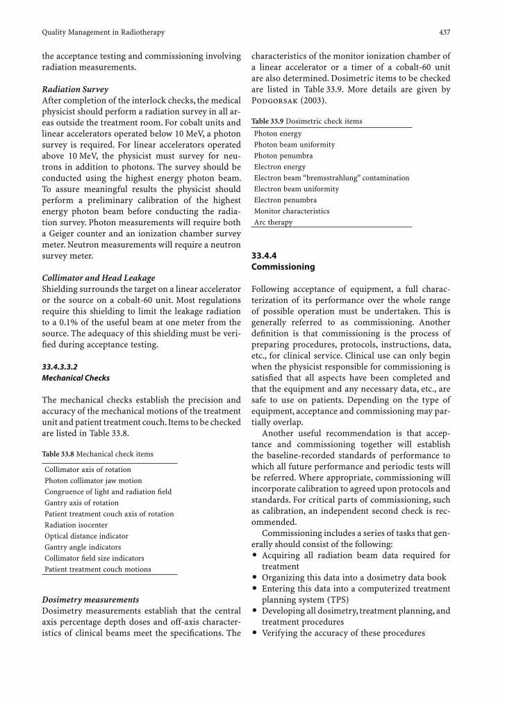
Quality Management in Radiotherapy 437

the acceptance testing and commissioning involving radiation measurements.

Radiation SurveyAfter completion of the interlock checks, the medical physicist should perform a radiation survey in all ar-eas outside the treatment room. For cobalt units and linear accelerators operated below 10 MeV, a photon survey is required. For linear accelerators operated above 10 MeV, the physicist must survey for neu-trons in addition to photons. The survey should be conducted using the highest energy photon beam. To assure meaningful results the physicist should perform a preliminary calibration of the highest energy photon beam before conducting the radia-tion survey. Photon measurements will require both a Geiger counter and an ionization chamber survey meter. Neutron measurements will require a neutron survey meter.

Collimator and Head LeakageShielding surrounds the target on a linear accelerator or the source on a cobalt-60 unit. Most regulations require this shielding to limit the leakage radiation to a 0.1% of the useful beam at one meter from the source. The adequacy of this shielding must be veri-fi ed during acceptance testing.

33.4.3.3.2 Mechanical Checks

The mechanical checks establish the precision and accuracy of the mechanical motions of the treatment unit and patient treatment couch. Items to be checked are listed in Table 33.8.

Table 33.8 Mechanical check items

Collimator axis of rotationPhoton collimator jaw motionCongruence of light and radiation fi eldGantry axis of rotationPatient treatment couch axis of rotationRadiation isocenterOptical distance indicatorGantry angle indicatorsCollimator fi eld size indicatorsPatient treatment couch motions

Dosimetry measurementsDosimetry measurements establish that the central axis percentage depth doses and off-axis character-istics of clinical beams meet the specifi cations. The

characteristics of the monitor ionization chamber of a linear accelerator or a timer of a cobalt-60 unit are also determined. Dosimetric items to be checked are listed in Table 33.9. More details are given by Podgorsak (2003).

Table 33.9 Dosimetric check items

Photon energyPhoton beam uniformityPhoton penumbraElectron energyElectron beam “bremsstrahlung” contaminationElectron beam uniformityElectron penumbraMonitor characteristicsArc therapy

33.4.4 Commissioning

Following acceptance of equipment, a full charac-terization of its performance over the whole range of possible operation must be undertaken. This is generally referred to as commissioning. Another defi nition is that commissioning is the process of preparing procedures, protocols, instructions, data, etc., for clinical service. Clinical use can only begin when the physicist responsible for commissioning is satisfi ed that all aspects have been completed and that the equipment and any necessary data, etc., are safe to use on patients. Depending on the type of equipment, acceptance and commissioning may par-tially overlap.

Another useful recommendation is that accep-tance and commissioning together will establish the baseline-recorded standards of performance to which all future performance and periodic tests will be referred. Where appropriate, commissioning will incorporate calibration to agreed upon protocols and standards. For critical parts of commissioning, such as calibration, an independent second check is rec-ommended.

Commissioning includes a series of tasks that gen-erally should consist of the following:• Acquiring all radiation beam data required for

treatment• Organizing this data into a dosimetry data book• Entering this data into a computerized treatment

planning system (TPS)• Developing all dosimetry, treatment planning, and

treatment procedures• Verifying the accuracy of these procedures

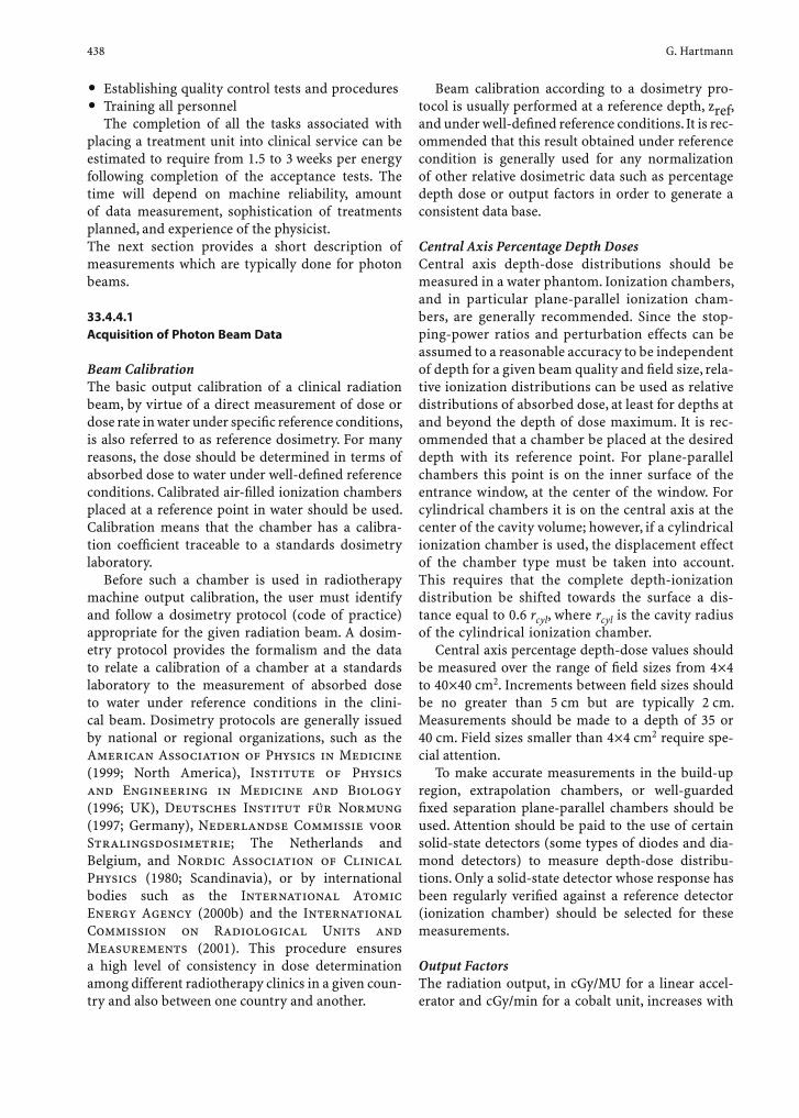
438 G. Hartmann

• Establishing quality control tests and procedures• Training all personnel

The completion of all the tasks associated with placing a treatment unit into clinical service can be estimated to require from 1.5 to 3 weeks per energy following completion of the acceptance tests. The time will depend on machine reliability, amount of data measurement, sophistication of treatments planned, and experience of the physicist.The next section provides a short description of measurements which are typically done for photon beams.

33.4.4.1 Acquisition of Photon Beam Data

Beam CalibrationThe basic output calibration of a clinical radiation beam, by virtue of a direct measurement of dose or dose rate in water under specifi c reference conditions, is also referred to as reference dosimetry. For many reasons, the dose should be determined in terms of absorbed dose to water under well-defi ned reference conditions. Calibrated air-fi lled ionization chambers placed at a reference point in water should be used. Calibration means that the chamber has a calibra-tion coeffi cient traceable to a standards dosimetry laboratory.

Before such a chamber is used in radiotherapy machine output calibration, the user must identify and follow a dosimetry protocol (code of practice) appropriate for the given radiation beam. A dosim-etry protocol provides the formalism and the data to relate a calibration of a chamber at a standards laboratory to the measurement of absorbed dose to water under reference conditions in the clini-cal beam. Dosimetry protocols are generally issued by national or regional organizations, such as the American Association of Physics in Medicine (1999; North America), Institute of Physics and Engineering in Medicine and Biology (1996; UK), Deutsches Institut für Normung (1997; Germany), Nederlandse Commissie voor Stralingsdosimetrie; The Netherlands and Belgium, and Nordic Association of Clinical Physics (1980; Scandinavia), or by international bodies such as the International Atomic Energy Agency (2000b) and the International Commission on Radiological Units and Measurements (2001). This procedure ensures a high level of consistency in dose determination among different radiotherapy clinics in a given coun-try and also between one country and another.

Beam calibration according to a dosimetry pro-tocol is usually performed at a reference depth, zref, and under well-defi ned reference conditions. It is rec-ommended that this result obtained under reference condition is generally used for any normalization of other relative dosimetric data such as percentage depth dose or output factors in order to generate a consistent data base.

Central Axis Percentage Depth DosesCentral axis depth-dose distributions should be measured in a water phantom. Ionization chambers, and in particular plane-parallel ionization cham-bers, are generally recommended. Since the stop-ping-power ratios and perturbation effects can be assumed to a reasonable accuracy to be independent of depth for a given beam quality and fi eld size, rela-tive ionization distributions can be used as relative distributions of absorbed dose, at least for depths at and beyond the depth of dose maximum. It is rec-ommended that a chamber be placed at the desired depth with its reference point. For plane-parallel chambers this point is on the inner surface of the entrance window, at the center of the window. For cylindrical chambers it is on the central axis at the center of the cavity volume; however, if a cylindrical ionization chamber is used, the displacement effect of the chamber type must be taken into account. This requires that the complete depth-ionization distribution be shifted towards the surface a dis-tance equal to 0.6 rcyl, where rcyl is the cavity radius of the cylindrical ionization chamber.

Central axis percentage depth-dose values should be measured over the range of fi eld sizes from 4×4 to 40×40 cm2. Increments between fi eld sizes should be no greater than 5 cm but are typically 2 cm. Measurements should be made to a depth of 35 or 40 cm. Field sizes smaller than 4×4 cm2 require spe-cial attention.

To make accurate measurements in the build-up region, extrapolation chambers, or well-guarded fi xed separation plane-parallel chambers should be used. Attention should be paid to the use of certain solid-state detectors (some types of diodes and dia-mond detectors) to measure depth-dose distribu-tions. Only a solid-state detector whose response has been regularly verifi ed against a reference detector (ionization chamber) should be selected for these measurements.

Output FactorsThe radiation output, in cGy/MU for a linear accel-erator and cGy/min for a cobalt unit, increases with

Quality Management in Radiotherapy 439

an increase in collimator opening or fi eld size. The output factor is determined as the ratio of corrected dosimeter readings measured under a given set of non-reference conditions to that measured under reference conditions, typically a 10×10-cm2 fi eld. Special attention should be given to the uniformity of the radiation fl uence over the chamber cavity. This is especially important for fi eld sizes smaller than 5×5 cm. Some accelerators have very pronounced V-shaped photon beam profi les which usually vary with depth and fi eld size. For large detectors it may be dif-fi cult to accurately correct for this variation. Thimble chambers with large cavity length and plane-paral-lel chambers with large collecting electrodes should therefore be avoided in situations where the beams have pronounced V-shaped profi les.

Output factors are usually given as a function of equivalent square fi elds. This approach assumes the output for rectangular fi elds is equal to the output of its equivalent square fi eld. This assumption must be verifi ed by measuring the output for a number of rectangular fi elds at their zmax. If the outputs of rectangular fi elds vary from the output of their equivalent square fi eld by more than 2%, it may be necessary to have a table or graph of output factors for each rectangular fi eld. The output of a rectangu-lar fi eld may also depend on whether the upper or lower jaw forms the long side of the fi eld. This effect is sometimes referred to as the collimator exchange effect and should be investigated as part of the com-missioning process.

There are two other collimator-dependent quan-tities: the collimator scatter factor and the phantom scatter factor. The collimator scatter factor is mea-sured “in air” with a build-up cap large enough to provide electronic equilibrium. Typically, these val-ues are normalized to a 10×10-cm2 fi eld.

A problem arises for small high-energy photon fi eld sizes as the size of the build-up cap approaches or exceeds the size of the fi eld. In this case the col-limator scatter correction factor may be determined by placing the ionization chamber at an extended shaded-surface display (SSD) but with the fi eld de-fi ned at the nominal SSD. With the chamber at 200 cm the collimator scatter correction factor can be mea-sured for fi elds with dimensions down to 4×4 cm2 at 100 cm. These relative measurements should all be performed under the same conditions.

As the output factor is the product of the collima-tor scatter correction factor and the phantom scatter correction factor, the phantom scatter correction fac-tor may be found by dividing the output factor by the collimator scatter correction factor.

Blocking Tray FactorsHigh-density shielding blocks are normally sup-ported on a plastic tray to correctly position them within the radiation fi eld can be used to protect normal critical structures within the irradiated area. This tray attenuates the radiation beam. The amount of beam attenuation provided by the tray must be known to calculate the dose received by the patient. The attenuation for solid trays is easily measured by placing an ionization chamber on the central axis of the beam at reference depth in phantom in a 10×10-cm2 fi eld. The ratio of the ionization chamber signal with the tray in the beam to the signal without the tray is the blocking tray transmission factor.

Multileaf CollimatorsOn most current treatment machines multileaf col-limators (MLC) are fi nding widespread application. One must differentiate between add-on MLCs and those MLC systems replacing at least one set of con-ventional jaws. For add-on MLCs, the central axis per-centage depth doses, the penumbra, and the output factor should be measured for a set of MLC-defi ned fi elds.

Leakage through the MLC consists of transmis-sion through the leaves and leakage between the leaves. Leakage between the leaves is easily demon-strated by exposing a fi lm placed perpendicularly to the collimator axis of rotation with the leaves fully closed. Leakage through the leaves can be determined by comparing the umbra region of transverse beam profi les for fi elds defi ned by the MLC to fi elds defi ned by the collimator jaws.

Central axis Wedge Transmission FactorsIn wedged photon beams the radiation intensity var-ies strongly in the direction of the wedge. For output measurements in such beams the detector dimension in the wedge direction should be as small as possible. A small thimble chamber aligned with its axis per-pendicular to the wedge direction is recommended. The coincidence of the central axes of the beam, the collimator, and the wedge should be ensured prior to making the output measurements.

The central axis wedge transmission factor is the ratio of the dose (or dosimeter reading) at a speci-fi ed depth on the central axis of a specifi ed fi eld size with the wedge in the beam to the dose for the same conditions without the wedge in the beam. Central axis wedge transmission factors determined for one fi eld size at one depth are frequently used to calculate beam-on time or monitor unit settings for all wedged fi elds and depths; however, the central axis wedge

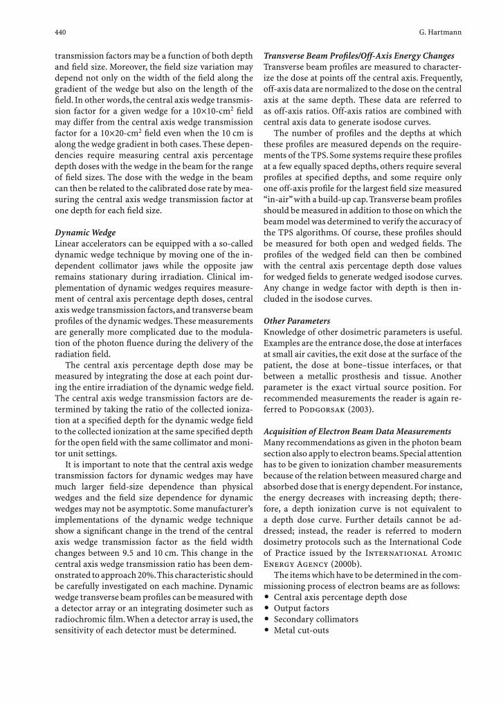
440 G. Hartmann

transmission factors may be a function of both depth and fi eld size. Moreover, the fi eld size variation may depend not only on the width of the fi eld along the gradient of the wedge but also on the length of the fi eld. In other words, the central axis wedge transmis-sion factor for a given wedge for a 10×10-cm2 fi eld may differ from the central axis wedge transmission factor for a 10×20-cm2 fi eld even when the 10 cm is along the wedge gradient in both cases. These depen-dencies require measuring central axis percentage depth doses with the wedge in the beam for the range of fi eld sizes. The dose with the wedge in the beam can then be related to the calibrated dose rate by mea-suring the central axis wedge transmission factor at one depth for each fi eld size.

Dynamic WedgeLinear accelerators can be equipped with a so-called dynamic wedge technique by moving one of the in-dependent collimator jaws while the opposite jaw remains stationary during irradiation. Clinical im-plementation of dynamic wedges requires measure-ment of central axis percentage depth doses, central axis wedge transmission factors, and transverse beam profi les of the dynamic wedges. These measurements are generally more complicated due to the modula-tion of the photon fl uence during the delivery of the radiation fi eld.

The central axis percentage depth dose may be measured by integrating the dose at each point dur-ing the entire irradiation of the dynamic wedge fi eld. The central axis wedge transmission factors are de-termined by taking the ratio of the collected ioniza-tion at a specifi ed depth for the dynamic wedge fi eld to the collected ionization at the same specifi ed depth for the open fi eld with the same collimator and moni-tor unit settings.

It is important to note that the central axis wedge transmission factors for dynamic wedges may have much larger fi eld-size dependence than physical wedges and the fi eld size dependence for dynamic wedges may not be asymptotic. Some manufacturer’s implementations of the dynamic wedge technique show a signifi cant change in the trend of the central axis wedge transmission factor as the fi eld width changes between 9.5 and 10 cm. This change in the central axis wedge transmission ratio has been dem-onstrated to approach 20%. This characteristic should be carefully investigated on each machine. Dynamic wedge transverse beam profi les can be measured with a detector array or an integrating dosimeter such as radiochromic fi lm. When a detector array is used, the sensitivity of each detector must be determined.

Transverse Beam Profi les/Off-Axis Energy ChangesTransverse beam profi les are measured to character-ize the dose at points off the central axis. Frequently, off-axis data are normalized to the dose on the central axis at the same depth. These data are referred to as off-axis ratios. Off-axis ratios are combined with central axis data to generate isodose curves.

The number of profi les and the depths at which these profi les are measured depends on the require-ments of the TPS. Some systems require these profi les at a few equally spaced depths, others require several profi les at specifi ed depths, and some require only one off-axis profi le for the largest fi eld size measured “in-air” with a build-up cap. Transverse beam profi les should be measured in addition to those on which the beam model was determined to verify the accuracy of the TPS algorithms. Of course, these profi les should be measured for both open and wedged fi elds. The profi les of the wedged fi eld can then be combined with the central axis percentage depth dose values for wedged fi elds to generate wedged isodose curves. Any change in wedge factor with depth is then in-cluded in the isodose curves.

Other ParametersKnowledge of other dosimetric parameters is useful. Examples are the entrance dose, the dose at interfaces at small air cavities, the exit dose at the surface of the patient, the dose at bone–tissue interfaces, or that between a metallic prosthesis and tissue. Another parameter is the exact virtual source position. For recommended measurements the reader is again re-ferred to Podgorsak (2003).

Acquisition of Electron Beam Data MeasurementsMany recommendations as given in the photon beam section also apply to electron beams. Special attention has to be given to ionization chamber measurements because of the relation between measured charge and absorbed dose that is energy dependent. For instance, the energy decreases with increasing depth; there-fore, a depth ionization curve is not equivalent to a depth dose curve. Further details cannot be ad-dressed; instead, the reader is referred to modern dosimetry protocols such as the International Code of Practice issued by the International Atomic Energy Agency (2000b).

The items which have to be determined in the com-missioning process of electron beams are as follows:• Central axis percentage depth dose• Output factors• Secondary collimators• Metal cut-outs

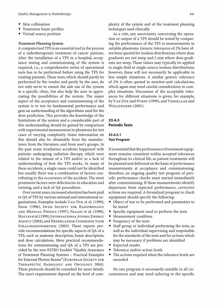
Quality Management in Radiotherapy 441

• Skin collimation• Transverse beam profi les• Virtual source position

Treatment Planning SystemA computerized TPS is an essential tool in the process of a radiotherapeutic treatment of cancer patients. After the installation of a TPS in a hospital, accep-tance testing and commissioning of the system is required, i.e., a comprehensive series of operational tests has to be performed before using the TPS for treating patients. These tests, which should partly be performed by the vendor and partly by the user, do not only serve to ensure the safe use of the system in a specifi c clinic, but also help the user in appre-ciating the possibilities of the system. The major aspect of the acceptance and commissioning of the system is to test its fundamental performance and gain an understanding of the algorithms used for the dose prediction. This provides the knowledge of the limitations of the system and a considerable part of this understanding should be gained by comparison with experimental measurement in phantoms for test cases of varying complexity. Some information on this should also be obtainable from the manufac-turer, from the literature, and from user’s groups. In the past some irradiation accidents happened with patients undergoing radiation therapy, which were related to the misuse of a TPS and/or to a lack of understanding of how the TPS works. In many of these accidents, a single cause could not be identifi ed but usually there was a combination of factors con-tributing to the occurrence of the accident. The most prominent factors were defi ciencies in education and training, and a lack of QA procedures.

Over recent years, increased attention has been paid to QA of TPS by various national and international or-ganizations. Examples include Van Dyk et al. (1999), Shaw (1996), Swiss Society for Radiobiology and Medical Physics (1997), Fraass et al. (1998), Mayles et al. (1999), International Atomic Energy Agency (2004), and Nederlandse Commissie voor Stralingsdosimetrie (2003). These reports pro-vide recommendations for specifi c aspects of QA of a TPS, such as anatomy description, beam description, and dose calculations. More practical recommenda-tions for commissioning and QA of a TPS are pro-vided by the new ESTRO booklet “Quality Assurance of Treatment Planning Systems – Practical Examples for External Photon Beams” (European Society for Therapeutic Radiology and Oncology 2004). These protocols should be consulted for more details. The exact requirements depend on the level of com-

plexity of the system and of the treatment planning techniques used clinically.

As a rule, any uncertainty concerning the opera-tion or output of a TPS should be tested by compar-ing the performance of the TPS to measurements in suitable phantoms. Generic tolerances of 2% have of-ten been quoted for isodose distributions where dose gradients are not steep and 2 mm where dose gradi-ents are steep. These values may typically be applied to single-fi eld or single-source isodose distributions; however, these will not necessarily be applicable in less simple situations. A similar generic tolerance of 2% is often quoted in monitor-unit calculations, which again may need careful consideration in com-plex situations. Discussion of the acceptable toler-ances for different situations is given, for example, by Van Dyk and Purdy (1999), and Venselaar and Welleweerd (2001).

33.4.5 Periodic Tests

33.4.5.1 Test Program

It is essential that the performance of treatment equip-ment remains consistent within accepted tolerances throughout its clinical life, as patient treatments will be planned and delivered on the basis of performance measurements at acceptance and commissioning; therefore, an ongoing quality test program of peri-odic performance checks must started immediately after commissioning. If these measurements identify departures from expected performance, corrective actions are required. A formalized program to check equipment should specify the following:• Object of test to be performed and parameters to

be tested• Specifi c equipment used to perform the tests• Measurement condition• Frequency of the tests• Staff group or individual performing the tests, as

well as the individual supervising and responsible for the standards of the tests and for actions which may be necessary if problems are identifi ed

• Expected results• Tolerance and/or action levels• The actions required when the tolerance levels are

exceeded

No one program is necessarily suitable in all cir-cumstances and may need tailoring to the specifi c

442 G. Hartmann

equipment and the departmental situation. For example, programs must be fl exible for additional testing whenever it seems necessary, following re-pair, observed equipment behavior, or indications of problems from the periodic tests. Also, frequen-cies may need to be adjusted in the light of experi-ence with a given machine. Staff resources available to undertake the program may limit what can be checked, which may have an effect on the structure of the test program. Tests should be designed to pro-vide the required information as rapidly as possible with minimal time and equipment. Often custom-ized devices are very useful to make tests easier. Examples of periodic tests are given in more detail for linear accelerators and for a TPS in the subsec-tions below.

34,4.5.2 Uncertainties, Tolerances, and Action Levels

In relevant documents, such as the “Guide to the Expression of Uncertainty in Measurement” (Inter-national Organization for Standardization 1993), uncertainties are classifi ed according to the method of evaluation as either type A, meaning that they have been assessed by statistical analysis of se-ries of observations, or type B, meaning that they have been assessed by other means. In the latter case the uncertainty is evaluated by scientifi c judgment based on all available information on the possible variability of the measured quantity. In previous text-books and still in common practice, uncertainties are frequently described as random (a posteriori) or systematic (a priori). Use of the type-A and type-B classifi cation is given preference. Irrespective of how uncertainties are assessed, the uncertainties at dif-ferent steps are usually combined in quadrature to estimate overall values.

For communicating uncertainties in an unmis-takable way it is helpful to introduce the “standard uncertainty” which is that uncertainty expressed as a standard deviation. Uncertainties are also related to confi dence levels. To associate a specifi c level of confi dence with the range of uncertainty requires explicit or implicit assumptions regarding the prob-ability distribution of the measurement result. In many situations there are good reasons to justify the assumption of a Gaussian distribution. In this case the standard uncertainty is associated with a confi -dence level of 68%, whereas an uncertainty expressed by two standard deviations is associated with a 95% confi dence level. In radiotherapy, this 95% confi dence level is normally the goal.

If a measurement is performed appropriately, it is expected to give the best estimate of the particu-lar measured parameter; however, this will have an associated uncertainty, dependent on the measure-ment technique. Therefore, the tolerance set for the parameter must take into account the uncertainty of the measurement technique employed. If the mea-surement uncertainty is greater than the tolerance or action level set, then random variations in the mea-surement will lead to unnecessary intervention, in-creased downtime of equipment, and ineffi cient use of staff time. On the other hand, tolerances should be set with the aim of achieving the overall uncertainties desired in radiotherapy, which are of the order of 2.5–3.5% standard uncertainty. Variances of individual parameters can be combined in quadrature for com-bined factors and this can now be used to determine specifi c tolerance limits for individual parameters.

Action levels are related to tolerances. For exam-ple, action levels are often set at approximately twice the tolerance level, although some critical parame-ters may require tolerance and action levels to be set much closer to each other or even at the same value. What happens if a measurement falls between tol-erance and action level? For practical reasons some fl exibility in monitoring and adjustment is needed. For example, if a measurement on the constancy of dose/MU indicates a result between the tolerance and action levels, then it may be permissible to al-low clinical use to continue until this is confi rmed by measurements the next day before taking any further action. If repeated measurements remain consistently between tolerance and action levels, adjustment is required. Any measurement at any time outside the action level requires immediate investigation and, if confi rmed, rectifi cation.

Different sets of recommendations may use very different approaches to set tolerance levels and/or ac-tion levels, and this should be borne in mind in com-paring values from different sources; in some, the term tolerance level is used to indicate values that in others may be closer to action levels, i.e., some work-ers use the term tolerance to indicate levels at which adjustment or correction is necessary.

34.4.5.3 Periodic Tests for Linear Accelerators

As an example for periodic tests, a typical test program for linear accelerators as suggested by the American Association of Physics in Medicine (1994a) is listed in Table 33.10. The experimental techniques for performing these tests are not described. Techniques

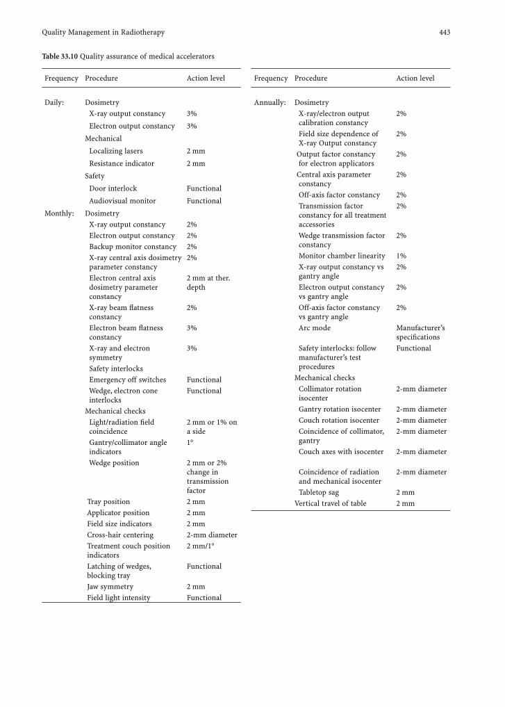
Quality Management in Radiotherapy 443

Table 33.10 Quality assurance of medical accelerators

Frequency Procedure Action level

Daily: Dosimetry X-ray output constancy 3%

Electron output constancy 3%

Mechanical

Localizing lasers 2 mm

Resistance indicator 2 mm

Safety

Door interlock Functional

Audiovisual monitor Functional

Monthly: Dosimetry X-ray output constancy 2% Electron output constancy 2% Backup monitor constancy 2% X-ray central axis dosimetry parameter constancy

2%

Electron central axis dosimetry parameter constancy

2 mm at ther. depth

X-ray beam fl atness constancy

2%

Electron beam fl atness constancy

3%

X-ray and electron symmetry

3%

Safety interlocks Emergency off switches Functional Wedge, electron cone interlocks

Functional

Mechanical checks Light/radiation fi eld coincidence

2 mm or 1% on a side

Gantry/collimator angle indicators

1°

Wedge position 2 mm or 2% change in transmission factor

Tray position 2 mm Applicator position 2 mm Field size indicators 2 mm Cross-hair centering 2-mm diameter Treatment couch position indicators

2 mm/1°

Latching of wedges, blocking tray

Functional

Jaw symmetry 2 mm Field light intensity Functional

Frequency Procedure Action level

Annually: Dosimetry X-ray/electron output calibration constancy

2%

Field size dependence of X-ray Output constancy

2%

Output factor constancy for electron applicators

2%

Central axis parameter constancy

2%

Off-axis factor constancy 2% Transmission factor constancy for all treatment accessories

2%

Wedge transmission factor constancy

2%

Monitor chamber linearity 1% X-ray output constancy vs gantry angle

2%

Electron output constancy vs gantry angle

2%

Off-axis factor constancy vs gantry angle

2%

Arc mode Manufacturer’s specifi cations

Safety interlocks: follow manufacturer’s test procedures

Functional

Mechanical checks Collimator rotation isocenter

2-mm diameter

Gantry rotation isocenter 2-mm diameter Couch rotation isocenter 2-mm diameter Coincidence of collimator, gantry

2-mm diameter

Couch axes with isocenter 2-mm diameter

Coincidence of radiation and mechanical isocenter

2-mm diameter

Tabletop sag 2 mmVertical travel of table 2 mm

444 G. Hartmann

as well as programs for other equipment, such as for cobalt-60 teletherapy machines, treatment simulators, CT scanners, or test equipment, can be adopted from a number of publications (American Association of Physics in Medicine 1994a, b; Wizenberg 1982; American National Standards Institute 1974, 1978). In Germany various periodic tests (so-called constancy tests) are explicitly described in part 5 of the respective German Standards (DIN).

Some comments have to be made to Table 33.10:• The level values listed in the third column should

be interpreted to mean real action levels.• For constancy, percent values are ± the deviation

of the parameter with respect its nominal value; distance values are referenced to the isocenter or nominal SSD.

• The electron output needs not to be checked daily for all electron energies, but all energies are to be checked at least twice weekly.

• Jaw difference is defi ned as difference in distance of each jaw from the isocenter, determined at the isocenter distance.

• Most wedge transmission factors are fi eld-size and depth dependent.

• The action level values for radiation output are 3% and 2% for daily and monthly checks, respec-tively. The 2% value for the monthly checks is given because these are normally performed with calibrated ionization chambers. The daily check, however, may also be performed by any device, which has at least the precision adequate to verify compliance with a tolerance value of 3%.

34.4.5.4 Periodic Tests for TPS

For safety and security reasons, periodic quality con-trol of particular parts of a TPS is also an important aspect of the QA process of a TPS. In this subsection tests are discussed that should be performed periodi-cally at specifi ed time intervals. For a software device, such as a TPS, one must be concerned about data fi les, integrity of the software executables, failures or problems in hardware peripherals and general sys-tem confi guration, as well as the process that uses the software. The main aims of a routine periodic QA program for the TPS include the following:• Confi rm the integrity and security of the TP data

fi les that contain the external beam and brachyther-apy information used in dose and MU calculations.

• Verify the correct functioning and accuracy of peripheral devices used for data input, including

the digitizer tablet, CT, MR, video digitizer, simu-lator control system, and devices for obtaining mechanical simulator contours. One must sepa-rately consider the devices themselves and the net-works, tape drives, software, transfer programs, and other components, which are involved in the trans-fer of the information from the device to the TPS.

• Check the integrity of the actual TPS software.• Confi rm the function and accuracy of output

devices and software, including printers, plot-ters, automated transfer processes, connections to computer-controlled block cutters, and/or com-pensator makers, etc.

The AAPM Radiation Therapy Committee Task Group 53 (Fraass et al. 1998) has given recommenda-tions on periodic tests of a TPS as specifi ed in Table 33.11. Commercial manufacturers often make their own rec-ommendations regarding ongoing QA of their planning systems. Each radiation oncology physicist should re-view all the recommendations and develop a program of periodic testing that will match the planning system characteristics and its user base. The frequency of test-ing of each specifi c feature of the RTP system should depend on how that feature is used in the clinic and how critical that feature is from a safety point of view.A series of reviews and training sessions is recom-mended to be included as part of the periodic QA program.

33.5 Clinical Aspects of QA

According to report of AAPM Radiation Therapy Committee Task Group 40 (American Association of Physics in Medicine 1994a), the method of peer review is particularly helpful in establishing a QA program for the clinical aspects. The three impor-tant components of such peer review are: new plan-ning conference; chart review; and fi lm/image review. Although already thoroughly discussed in the report, the essential steps to perform such peer reviews are briefl y described in the following subsection.

33.5.1 New Patient Planning Conference

New patient planning conference should be attended by radiation oncologists, radiation therapists, and medical physicists. In some countries, such as the

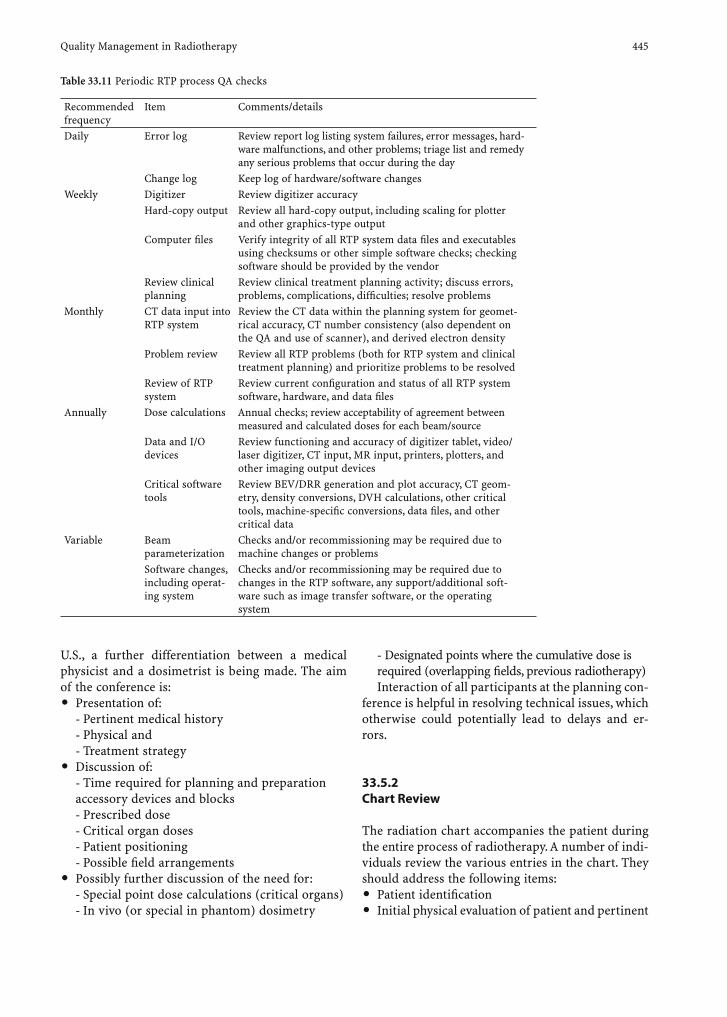
Quality Management in Radiotherapy 445

U.S., a further differentiation between a medical physicist and a dosimetrist is being made. The aim of the conference is:• Presentation of:

- Pertinent medical history- Physical and - Treatment strategy

• Discussion of:- Time required for planning and preparation accessory devices and blocks- Prescribed dose- Critical organ doses- Patient positioning- Possible fi eld arrangements

• Possibly further discussion of the need for:- Special point dose calculations (critical organs)- In vivo (or special in phantom) dosimetry

- Designated points where the cumulative dose is required (overlapping fi elds, previous radiotherapy)Interaction of all participants at the planning con-

ference is helpful in resolving technical issues, which otherwise could potentially lead to delays and er-rors.

33.5.2 Chart Review

The radiation chart accompanies the patient during the entire process of radiotherapy. A number of indi-viduals review the various entries in the chart. They should address the following items:• Patient identifi cation• Initial physical evaluation of patient and pertinent

Table 33.11 Periodic RTP process QA checks

Recommended frequency

Item Comments/details

Daily Error log Review report log listing system failures, error messages, hard-ware malfunctions, and other problems; triage list and remedy any serious problems that occur during the day

Change log Keep log of hardware/software changesWeekly Digitizer Review digitizer accuracy

Hard-copy output Review all hard-copy output, including scaling for plotter and other graphics-type output

Computer fi les Verify integrity of all RTP system data fi les and executables using checksums or other simple software checks; checking software should be provided by the vendor

Review clinical planning

Review clinical treatment planning activity; discuss errors, problems, complications, diffi culties; resolve problems

Monthly CT data input into RTP system

Review the CT data within the planning system for geomet-rical accuracy, CT number consistency (also dependent on the QA and use of scanner), and derived electron density

Problem review Review all RTP problems (both for RTP system and clinical treatment planning) and prioritize problems to be resolved

Review of RTP system

Review current confi guration and status of all RTP system software, hardware, and data fi les

Annually Dose calculations Annual checks; review acceptability of agreement between measured and calculated doses for each beam/source

Data and I/O devices

Review functioning and accuracy of digitizer tablet, video/laser digitizer, CT input, MR input, printers, plotters, and other imaging output devices

Critical software tools

Review BEV/DRR generation and plot accuracy, CT geom-etry, density conversions, DVH calculations, other critical tools, machine-specifi c conversions, data fi les, and other critical data

Variable Beam parameterization

Checks and/or recommissioning may be required due to machine changes or problems

Software changes, including operat-ing system

Checks and/or recommissioning may be required due to changes in the RTP software, any support/additional soft-ware such as image transfer software, or the operating system

446 G. Hartmann

clinical information• Treatment planning• Signed and witnessed consent form• Treatment execution• Clinical assessment during treatment• QA checklists

The authors of the report recommend that:• Charts be reviewed

- At least weekly- Before the third fraction following the start or

a fi eld modifi cation- At the completion of treatment

• The review be signed and dated by the reviewer• The QA team oversee the implementation of a

program which defi nes- Which items are to be reviewed- Who is to review them- When are they to be reviewed- The defi nition of minor and major errors- What actions are to be taken, and by whom, in

the event of errors• All errors be reviewed and discussed by the QA

team including Documentation ofConsequences

• A random sample of charts be audited at inter-vals prescribed by the QA team

33.5.3 Film/Image Review

The review of fi lms and/or digital images mainly re-fers to those obtained during the localization proce-dure using portal imaging and verifi cation imaging. Whereas a portal image is obtained by exposing the fi lm (or the image detector) to only a small fraction of the daily treatment dose, verifi cation images are single-exposure images that record the delivery of the entire dose for each fraction from each fi eld.

It is recommended that all initial portal images be reviewed, signed, and dated by the radiation oncolo-gist before the fi rst treatment for curative or special palliative irradiations, and before the second fraction for palliative irradiations.

A general recommendation on how often ongoing portal and verifi cation images should be produced and reviewed cannot be given. There are several stud-ies showing that clinically signifi cant localization changes (errors) frequently may occur, and that this frequency can be reduced by increasing the number of ongoing portal imaging; however, time and cost are still considerable obstacles to introduce at a daily

imaging procedure, and it would be worthwhile to always arrive at an well-controlled localization. New concepts, such as adaptive radiotherapy, are cur-rently being developed to overcome this problem of resources. The AAPM report recommends that portal or verifi cation images of all fi elds be obtained at least once a week.

References

American Association of Physics in Medicine (1984) Physical aspects of quality assurance in radiation therapy. Report series no. 13. American Institute of Physics, New York

American Association of Physics in Medicine (1994a) Com-prehensive QA for radiation oncology. Report of AAPM Radiation Therapy Committee Task Group 40. Med Phys 21:581–618

American Association of Physics in Medicine (1994b) Code of practice for accelerators. Report of AAPM Radiation Ther-apy Committee Task Group 45 Med Phys 21:1093–1121

American Association of Physics in Medicine (1999) Task Group 51. Protocol for clinical reference dosimetry of high-energy photon and electron beams. Med Phys 26:1847–1870

American National Standards Institute (1974) Guidelines for maintaining Co-60 and Cs-137 teletherapy equipment. Report no. 449. American National Standards Institute, Washington DC

American National Standards Institute (1978) Procedures for periodic inspection of Co-60 and Cs-137 teletherapy equipment. Report no. 449.1. American National Standards Institute

Brahme A, Chavaudra J, Landberg T, McCullough E, Nüsslin F, Rawlinson A, Svensson G, Svensson H (1988) Accuracy requirements and quality assurance of external beam ther-apy with photons and electrons. Acta Oncol 27 (Suppl 1)

Deutsches Institut für Normung (1997) Dosismessverfahren nach der Sondenmethode für Photonen- und Elektronen-strahlung, Teil 2: Ionisationsdosimetrie. Deutsche Norm DIN 6800-2, Deutsches Institut für Normung, Berlin

Dobbs H, Thwaites DI (1999) Quality assurance and its con-ceptual framework. Institute of Physics and Engineering in Medicine, York, UK, Chap. 1

Dutreix A (1984) When and how can we improve precision in radiotherapy? Radiother Oncol 2:275–292

European Society for Therapeutic Radiology and Oncology (2004) Quality assurance of treatment planning systems: practical examples for external photon beams. ESTRO, Brussels, booklet no. X

Fraass B, Doppke K, Hunt M, Kutcher G, Starkschall G, Stern R, Van Dyk J (1998) American Association of Physicists in Medicine Radiation Therapy Committee Task Group 53: Quality assurance for clinical radiotherapy treatment plan-ning. Med Phys 25:1773–1836

Institute of Physics and Engineering in Medicine and Biol-ogy (1996) The IPEMB code of practice for the determina-tion of absorbed dose for X-rays below 300 kV generating potential (0.035 mm Al–4 mm Cu; 10–300 kV generating potential). Phys Med Biol 41:2605–2625

International Atomic Energy Agency (1999) Standardized quality audit procedures for on-site dosimetry visits to

Quality Management in Radiotherapy 447

radiotherapy hospitals. IAEA DMRP-199907-IU. Interna-tional Atomic Energy Agency, Vienna

International Atomic Energy Agency (2000a) Lessons learned from accidental exposures in radiotherapy. Safety Reports Series no. 17. International Atomic Energy Agency, Vienna

International Atomic Energy Agency (2000b) Absorbed dose determination in external beam radiotherapy: an interna-tional code of practice for dosimetry based on standards of absorbed dose to water. Technical report series no. 398. International Atomic Energy Agency, Vienna

International Atomic Energy Agency (2004) Commissioning and quality assurance of computerized treatment plan-ning. Technical Report Series no. 430. International Atomic Energy Agency, Vienna

International Commission on Radiological Units and Mea-suremenets (1976) Determination of dose in a patient irradiated by beams of X or gamma rays in radiotherapy procedures. ICRU report 24. ICRU, Bethesda, Maryland

International Commission on Radiological Units and Mea-surements (2001) Dosimetry of high-energy photon beams based on standards of absorbed dose to water. ICRU report 64. J ICRU 1

International Electrotechnical Commission (1989a) Medical electrical equipment: medical electron accelerators – func-tional performance characteristics. IEC 976. International Electrotechnical Commission, Geneva, Switzerland

International Electrotechnical Commission (1989b) Medical electrical equipment: medical electron accelerators in the range 1 MeV to 50 MeV – guidelines for performance char-acteristics. IEC 977. International Electrotechnical Com-mission, Geneva, Switzerland

International Organisation for Standardization (1993) Guide to the expression of uncertainty in measurement. Interna-tional Organisation for Standardization, Geneva, Switzer-land

Leer JW, Corver R, Kraus JJ, Togt JC, Buruma OJ (1995) A quality assurance system based on ISO standards: expe-rience in a radiotherapy department. Radiother Oncol 35:75–81

Leer JW, McKenzie AL, Scalliet P, Thwaites DI (1998) Practical guidelines for the implementation of a quality system in radiotherapy. European Society for Therapeutic Radiology and Oncolgy. Physics for Clinical Radiotherapy, booklet no. 4. ESTRO, Brussels

Mayles WPM, Lake R, McKenzie A, Macaulay EM, Morgan HM, Jordan TJ, Powley SK (eds) (1999) Physics aspects of quality control in radiotherapy. IPEM report 81. Institute of Phys-ics and Engineering in Medicine, York, UK

McKenzie A, Kehoe T, Thwaites DI (2000) Quality assurance in radiotherapy physics. In: Williams JR, Thwaites DI (eds) Radiotherapy physics in practice. Oxford Medical Publish-ing, Oxford

Mijnheer B, Battermann J, Wambersie A (1987) What degree of accuracy is required and can be achieved in photon and neutron therapy. Radiother Oncol 8:237–252

Nederlandse Commissie voor Stralingsdosimetrie (1997) Dosimetry of low and medium energy X-rays, a code of practice for use in radiotherapy and radiobiology, report NCS-10. NCS, Delft, The Netherlands

Nederlandse Commissie voor Stralingsdosimetrie (2003) Quality assurance of 3-D treatment planning systems; practical guidelines for acceptance testing, commissioning, and periodic quality control of radiation therapy treatment planning systems. The Netherlands Commission on Radia-tion Dosimetry. Delft, The Netherlands

Nordic Association of Clinical Physics (1980) Procedures in external radiation therapy dosimetry with electron and photon beams with maximum energies between 1 and 50 MeV. Acta Radiol Oncol 19:55–79

Podgorsak EB (ed) (2003) Review of radiation oncology phys-ics: a handbook for teachers and students. Educational Reports Series. International Atomic Energy Agency, Vienna

Shaw JE (ed) (1996) A guide to commissioning and quality con-trol of treatment planning systems. IPEM report 68. Insti-tute of Physics and Engineering in Medicine, York, UK

SSRPM Report 7 (1997) Quality control of treatment planning systems for teletherapy. Swiss Society for Radiobiology and Medical Physics: ISBN 3-908125-23-5

Thwaites D, Scalliet P, Leer JW, Overgaard J (1995) Quality assurance in radiotherapy. European Society for Thera-peutic Radiology and Oncology Advisory Report to the Commission of the European Union for the Europe Against Cancer Programme. Radiother Oncol 35:61–73

Van Dyk J (ed) (1999) Radiation oncolgy overview. In: The modern technology for radiation oncology: a compendium for medical physicists and radiation oncologists. Medical Physics Publishing, Madison, Wisconsin

Van Dyk J, Purdy J (1999) Clinical implementation of technol-ogy and the quality assurance process. In: Van Dyk J (ed) The modern technology for radiation oncology: a com-pendium for medical physicists and radiation oncologists. Medical Physics Publishing, Madison, Wisconsin, pp 19–52

Van Dyk J, Barnett RB, Cygler JE, Shragge PC (1993) Com-missioning and quality assurance of treatment planning computers. Int J Radiat Oncol Biol Phys 26:261–273

Venselaar JLM, Welleweerd J (2001) Application of a test pack-age in an intercomparison of the performance of treatment planning systems used in a clinical setting. Radiother Oncol 60:203–213

Wizenberg MJ (ed) (1982) Quality assurance in radiation therapy: a manual for technologists. American College of Radiology, Philadelphia

World Health Organization (1988) Quality assurance in radio-therapy. WHO, Geneva, Switzerland

Subject Index 449

Subject Index

CMYK

A/ ratio 231/ value 224

abdominal compression 278acceptance test 436accidents 427ACR, see American College of Radiologyaction level 435, 442active– breathing control 279, 308– contour 23– source length 389, 391– tracking 340adaptive radiotherapy 2, 5advanced single-slice rebinning (ASSR) 71, 72AEC, see automatic exposure controlaffi ne transformation 44air kerma strength 243algebraic reconstruction 12algorithm– convolution 191– dose optimization 380– evolutionary 248– genetic 248, 380– gradient-based optimization 248– histogram-reduction 226– linear optimization 213– marching cubes 24, 25– of Feldkamp 71– of Monte Carlo 197, 198– optimization 212– pencil beam 188, 190, 197, 356– ray-tracing 183– region growing 21– shear warp 26– superposition 191, 194– tracking-based 25American Association of Physics in Medicine Radiation

Therapy Committee Task Group 430American College of Radiology (ACR) 54– NEMA 55anatomical atlas 24– 3D 37angiogram 390angioplasty 390, 391anisotropy function 244anthropomorphic phantom 416aperture design 433archiving 58arterio-venous malformation (AVM) 106–108, 110, 271ASSR, see advanced single-slice rebinning

atlas 37ATSM-PET 173automated image pre-processing 23automatic exposure control (AEC) 74AVM, see arterio-venous malformation

Bballoon implantation 398– MammoSite RTS 403balloon-cavity conformance 404bang gel 415baseline value 435basic dosimetry for dose algorithm production 412beam– angles 212– calibration 438– eye view 181– monitoring 352– orientation 212beam-shaping device 257BED, see biologically effective dosebiological– imaging 175– model 221– target volume 168, 170– treatment planning 379biologically effective dose (BED) 224block format 53blocking tray factor 439blood oxygen level dependent (BOLD) 106, 110– contrast 104, 105– venography 107, 108boundary tracking 22brachytherapy 5, 237– coronary 393– interstitial 398– intravascular, based on beta sources 393– partial breast 397– permanent implant 379– vascular 389Bragg peak 205, 345, 365brain glioma 113, 115breath-hold technique 279, 305breathing motion 337B-spline transformation 45BTV 175

CCanny operator 22cell survival after charged particle irradiation 230centering balloon 393

450 Subject Index

CMYK

central axis– percentage depth 438, 440– wedge transmission factor 439CGE, see Cobalt Gray equivalentchain– of procedures 432– of radiotherapy 2chamber phantom 416charged particle– irradiation– – cell survival 230– therapy 5chart review 445choline (Cho) 116chondrosarcoma 373chordoma 373classifi cation method 21claudication 393clinical– evaluation 432– target length 391– target volume (CTV) 168, 175, 251Cobalt Gray equivalent (CGE) 229COIN, see conformal indexcollapsed cone 192collimator– and head leakage 437– axis of rotation 437– fi eld size indicator 437– scatter factor (CSF) 189colour-wash technique 184commissioning 437Committee Radiological Oncology (ARO) 431comprehensive quality management program 429Compton scatter 199cone-beam– CT 70– reconstruction 11conformal– index (COIN) 251, 252– radiotherapy 2conformational radiation therapy (CRT) 257congruence of light and radiation fi eld 437constraint 208, 209convergence error 194convolution algorithm 191coronary brachytherapy 393cosmetic result 405costlet 209CRE, see cumulative radiation effectcreatine (Cr) 116critical– element model 226– structures 167, 169– volume model 227CRT, see conformational radiation therapyCSF, see collimator scatter factorCT 257– 16-slice 77– 4D 83, 85, 86, 305, 307– calibration 202– cone beam 71– gated 77, 83

– helical 93– number 32– values 69Cu-ATSM 134, 141, 144cumulative radiation effect (CRE) 223Cyberknife 338– Image-Guided Radiosurgery System 278cyclotron 349– isochronous 349cylindrical solid water phantom 415

Ddata– format 53– fusion 49density scaling 192department‘s policy formulation 430depth dose curve 189, 194detection of edges 22detector row 77diamond detector 419diaphragm 304DICOM 44, 54, 55, 58, 60, 63– RT 56, 57digital fi lter 201digitally reconstructed radiograph (DRR) 4, 29, 62, 183, 184,

342DIL, see dominant interprostatic lesiondistal edge tracking (DET) 358DLT, see magnetic tape storagedominant interprostatic lesion (DIL) 124, 125dose– algorithm production 412– calculation 4, 187– – accuracy 187, 202– – in brachytherapy 242– – of Monte Carlo 188– distribution– – 3D 4, 193– – computation 433– – display 184– evaluation in brachytherapy 250– homogeneity 209– kernel 188–190– mean dose 209– optimization– – algorithm 380– – in brachytherapy 246– physical criteria 209– prescribed and delivered 427– prescribed level 209– tolerance level 209dose-response curve 221, 226dose-volume– histogram (DVH) 169, 185, 209, 213– iso-effect curve 226dosimetry– measurement 437– verifi cation 432Douglas-Fowler plot 224DRR, see digitally reconstructed radiographDVH, see dose-volume histogramdynamic wedge 440

Subject Index 451

CMYK

EEA, see evolutionary algorithmecho-planar imaging (EPI) 102, 104, 105eddy currents 99effective dose 73electron– contamination 203– interaction 200– source 202– transport 199electronic portal images (EPI) 62, 413endorectal– coil 115– MRI 124endovascular brachytherapy (EVBT) 389energy– absorption 189– fl uence 190– spectrum 189EPI, see electronic portal images; echo-planar imagingEPID, see electronical portal imaging deviceequivalent– dose 222– uniform dose (EUD) 210, 217ERD, see extrapolated response doseerror 427ESTRO 434ethernet 54EUD, see equivalent uniform doseEVBT, see endovascular brachytherapyevolutionary algorithm (EA) 248external– fi ducial 338– marker 339extracranial– radiosurgery 278– stereotactic radiation therapy 277extrapolated response dose (ERD) 224

Ffan-beam reconstruction 10fat necrosis 404, 405FBP 70FDG, see fl uoro-deoxyglucosefeasability search 207Feldkamp algorithm 71ferrous sulphate gel 415fi ducial– external 338– internal 338– marker 46, 339fi ducial-based respiration– compensation 340– tracking 341fi lm 415– calibration condition 414– dosimetry 413, 414, 418– review 446fi lter 201fi ltered backprojection 11, 12, 69fi nite element method 326fi xed format 53FLAIR, see fl uid-attenuated inversion recovery

FLT 173fl uence 189– map 413– matrix 190– transmitted 413fl uid-attenuated inversion recovery (FLAIR) 114fl uoro-deoxyglucose (FDG) 140, 142– PET 134, 145, 170–172FMISO 173format– block 53– fi xed 53– graphic interchange (GIF) 54– JPEG fi le interchange (JIFF) 54– tag-/record-based 54– tagged image fi le (TIFF) 54forward treatment planning system 3, 213Fourier– projection 33– slice theorem 10– space 33fractionation 223– regime 225FSU, see functional subunitfunctional subunit (FSU) 226, 227

GGA, see genetic algorithmgamma knife 277gantry 351– angle indicator 437– axis of rotation 437– rotation 203gated CT 77, 83genetic algorithm (GA) 248, 380geometric transformation 43geometry factor 243German Association of Radiooncology (DEGRO) 431German Cancer Association 431GIF, see graphic interchange formatgold– fi ducial 304– marker 339gradient technique 212gradient-based optimization algorithm 248graphic interchange format (GIF) 54gross tumour volume (GTV) 168, 172, 175, 239, 251– nodal (GTV-N) 168– primary (GTV-P) 168GTV, see gross tumour volume

HHDR, see high dose ratehelical– CT 86, 93– scanning 82high dose rate (HDR) 242– brachytherapy 389high-LET radiation 229, 232high-pass fi ltering 19histogram-reduction algorithm 226Hounsfi eld 67, 69– number 188– unit 32, 180, 199

452 Subject Index

CMYK

hybrid phantom 412, 414hypofractionation 307hypoxia 133, 229

IICRU report– 24 426– 46 202– 50 167, 168, 175– 60 175– 62 167–169IGRT, see image-guided therapyimage– cube 180– distorsion 102– fusion 34– reconstruction 68, 71– registration 34, 42, 51– review 446image-guided therapy (IGRT) 5image-smoothing technique 19imaging– 3D 432– biological 175– tumour localization 3implanted seeds 244importance factor 209IMPT, see intensity-modulated proton therapyIMRT, see intensity-modulated radiotherapyinfrared– sensor technique 340– tracking 338–340in-stent restenosis in coronary arteries 390intelligent volume 37intensity level 212intensity-modulated– dosimetric verifi cation 411, 418– protocol 210– proton therapy (IMPT) 346, 348, 356, 357– quality assurance 414– – pre-treatment 412, 418– radiotherapy (IMRT) 5interaction– coeffi cient 201– process 199, 200interactive segmentation 25interlock 436internal– fi ducial 338– marker 339– target volume (ITV) 169, 175International Atomic Energy Agency 434Inter-Society Council for Radiation Oncology (ISCRO) 430interstitial brachytherapy– in partial breast irradiation 398intervention length 391intraoperative radiotherapy (IORT) 398intravascular brachytherapy based on beta sources 393inverse– planning 3, 204, 207, 247– – program 213– – software 411– problem 9

ion– beam therapy 205– chamber– – dosimetry 415– – solid water matrix phantom 416ionisation chamber 415, 428iridium-192 398, 399– source 389irradiated volume 168, 169ISDN communication 63isochronous cyclotron 349iso-dose line 184ITV, see internal target volume

Jjet ventilation 279JIFF, see JPEG fi le interchange formatJoint Commission on the Accreditation of Healthcare Organi-

zations (JCAHO) 430JPEG 59– fi le interchange format (JIFF) 54

Kkernel tilting 192kick-off time 223

Llactate 116LAN, see local area networklateral penumbra 189LDR, see low dose ratelesion length 391LET, see linear energy transferlinac– head geometry 202– isocentre adjustment 421– view 182linac-based QA 419linear– accelerator 277– energy transfer (LET) 222, 230, 360, 366– optimization algorithm 213– programming 213linear-quadratic model 223, 231lipid 116liquid ionisation chamber array 415liver tumor 282, 300local area network (LAN) 54, 59low dose rate (LDR) 242lucite cylinder phantom 415lung tumor 280, 300Lyman model 226, 227, 232Lyman-Kutcher model 225

Mmagnetic– resonance imaging (MRI) 172, 180, 257– – endorectal 124– – functional 104, 110– tape storage (DLT) 59mapping 50marching cubes algorithm 26, 27marker

Subject Index 453

CMYKCMYK

– external 339– internal 339mAs– product 72– value 72, 73mass density 202mathematical optimization 208matrix phantom 418maximum– intensity projection (MIP) 29, 184– likelihood classifi er 20MCD, see mean central doseMD-CRT, see multidimensional conformal radiotherapymean– central dose (MCD) 251– dose 209mechanical check 437median fi ltering 19Medical-Scientifi c Associations 431mega-voltage image 184metal cut-out 440Mick applicator 380micro-MLC 265MIDI 54minimum– peripheral dose (mPD) 380– target dose (MTD) 251MIP, see maximum intensity projectionMLC, see multi-leaf collimatormodality– performed procedure step (MPPS) 60– worklist management (MWL) 60modulation wheel 354Monte Carlo technique 200– algorithm 197, 198– dose calculation 188– – for inverse planning 204– dose engines 203– simulation 201, 203motion artifact 82moving target 2MPEG 54MPPS, see modality performed procedure stepMR spectroscopy (MRS) 172, 175, 379MRI, see magnetic resonance imagingMTD, see minimum target dosemulticriteria optimization 216multidimensional conformal radiotherapy (MD-CRT) 170multi-disciplinary process 425multi-leaf collimator (MLC) 5, 204, 257, 289, 413, 439– accessory type 260– confi guration in the treatment head 261– double-focussed 420– fi eld size 419– focusing properties 262– geometrical and mechanical properties 258– interdigitation 261– interleaf leakage 263– leaf transmission 263– leaf width 259– leaf-position accuracy test 419– leaf-speed test 419– leakage radiation 264

– maximum fi eld size 259– maximum overtravel 261– operating modes 265– optimum leaf width 260– transmitted intensity 264multimodality registration 51multiobjective optimization 247, 248– evolutionary algorithm 249multi-planar reconstruction 183multiple scattering 200multislice 76mutual information 35, 47MWL, see modality worklist management

NN-acetylasparatate (NAA) 116NAS, see network attached storageNational Electrical Manufacturers Association (NEMA) 54natural dose volume histogram (NDVH) 251NDVH, see natural dose volume histogramneck phantom 416needle insertion 239NEMA, see National Electrical Manufacturers Associationnetwork attached storage (NAS) 59neutrons 231, 360new patient planning conference 444nominal standard dose (NSD) 223non-coplanar beam 213non-rigid registration 94normal anatomy, delineation 180normal tissue (NT) 213, 246– probability 1, 208, 217, 221, 223, 379, 426– – model 225nozzle 352NSD, see nominal standard doseNT, see normal tissueNTCP, see normal tissue complication probability

OOAR, see organs at riskobjective function 209, 210, 247observer‘s view 181OER, see oxygen enhancement ratiooff-axis ratio 187open system interconnection (OSI) 54optical– distance indicator 437– guidance 157– – ultrasound 159– tracking 158optimization– algorithm 212– criteria 208– parameter 213organ– at risk (OAR) 2, 169, 170, 237– – localization 432– motion 278OSI, see open system interconnectionoutput factor 187, 438, 440oversampling 28oxygen enhancement ratio (OER) 229

454 Subject Index

CMYKCMYK

PPACS 54, 59pair production 199para-aortic lymph node (PALN) 144parallel-beam reconstruction 10paraspinal tumor 285Pareto optimal solution 216Paris system 398partial breast 399– brachytherapy 397– irradiation 398– – using high-dose-rate interstitial brachytherapy 401– – using low-dose-rate insterstitial brachytherapy 399particle– history 199– scanning technique 355passive scattering 353pathlength scaling 192patient– data acquisition 433– identifi cation 428– immobilization 139, 360, 433– monitoring equipment 436– positioning 4, 139, 360, 368, 432, 433– setup 44– treatment couch– – axis of rotation 437– – motion 437PDD, see percentage depth dose curvepenalty factor 209pencil beam 192– algorithm 188, 190, 197, 356percentage depth dose curve (PDD) 411percutaneous transluminal– angioplasty (PTA) 389– coronary angioplasty (PTCA) 389PEREGRINE system 204performance characteristic 435periodic test 441– for linear accelerator 442– for TPS 444permanent– implant brachytherapy 379– interstitional implantation 379PET, see positron emission tomographyphase space plan 202phosphorus-32 390photoelectric absorption 199photon– beam data 438– collimator jaw motion 437– fl uence 203– transport 199photon-energy spectrum 193pincushion distortion 99pitch value 70, 72plan– evaluation 433– implementation 433planning– organs at risk volume (PRV) 170– target length 390, 391– target volume (PTV) 2, 168, 169, 172, 237, 239, 251

PNG, see portable network graphicpoint matching 51policy manual 430portable network graphic (PNG) 54positron emission tomography (PET) 167, 180– MET 172– CT 43pre-procesing 18– automated image 24prescription 428, 433primary photons 189prostate 115, 122– brachytherapy 379, 380proton 345– accelerator 349PRV, see planning organs at risk volumepseudo-coloring 50PTA, see percutaneous transluminal angioplastyPTCA, see percutaneous transluminal coronary angioplastyPTV, see planning target volume

QQMS, see quality management systemQS, see quality systemquality– assurance (QA) 5, 411, 425– – clinical aspects 444– – protocol 435– audit 433– characteristic 435– management system (QMS) 426– manual 432– measurement– – project team 430– system (QS) 425, 427, 434– – structuring 430

Rradial– dose function 244– reference depth 391radiation– isocenter 437– measurement system 428– survey 437– treatment planning– – standards 175radioactive sources– beta 389– gamma 389radioisotopes 379– 125I 380– 103Pd 380radiosurgical treatment 421radiotherapy– adaptive 2– chain 2– conformal 2– intensity-modulated 5– intraoperative 398– multidimensional conformal (MD-CRT)– planning cycle 180random number 198

Subject Index 455

CMYKCMYK

range compensator 354raster scanning 355ray casting 29ray-tracing algorithm 183RBE, see relative biological effi ciencyRDDP, see reference depth dose pointreal-time position management (RPM) 302– system 84reconstruction– algebraic 12– cone beam 11– fan beam 10– multi-planar 183– parallel beam 10– simultaneous iterative technique 13record-and-verify system 57reference– depth dose point (RDDP) 391– isodose length (RIL) 391– lumen diameter (RLDi) 391– point 244region growing algorithm 20registration 24, 45– multimodality 51– non-rigid 94relative biological effi ciency (RBE) 222, 229, 230, 359, 365– clinical values 231– of high-LET radiation 232– variations for protons 232renal artery restenosis after dilatation 390respiratory– air fl ow 301– artifact 89, 93– gating 338– motion 337, 81restenosis prophylaxis 392retrospective sorting 85rigid transformation 46RIL, see reference isodose lengthRLDi, see reference lumen diameterrobotic gantry 340room laser adjustment 421, 422rotation 46– matrix 4332-row scanner 77RPM, see real-time position managementRTP fi le transfer quality assurance 412

Ssafety– characteristic 435– check 436SAN, see storage area networkSC, see storage commitmentscattering system 3533D scene 184scoring function 208SDP, see source dwell positionsecondary– collimator 440– electrons 193segmented multi-leaf modulation (SMLM) 412sharpening method 19

shear-warp algorithm 28signal-to-noise ratio (SNR) 68simulation 433simultaneous iterative reconstruction technique 13single– beam verifi cation 413, 415– objective problem 247– photon computed emission tomography 167, 180– – IMT 172skin collimation 441skin–balloon surface distance 404sliding window technique 265snake 22SNR, see signal-to-noise ratioSOBP, see spread-out Bragg-peaksolid water slab 415source dwell position (SDP) 246spatial model 37specifi c test characteristic 435SPECT, see single photon computed emission tomographySPGR, see spoiled gradient-echospinal tumor 285spiral CT 11, 70spirometry 301spline 44– transformation 44spoiled gradient-echo (SPGR) 114spot scanning 355– dynamic 355spread-out Bragg-peak (SOBP) 230, 353stationary random process 323step-and shoot– technique 290– IMRT 412, 418– mode 212, 265stereo X-ray imaging 338, 339stereotactic– body frame 277– coordinates 277– irradiation technique 265– radiation therapy– – fractionated 278– – frameless system 278stopping power 201storage– area network (SAN) 59– commitment (SC) 60strontium-90 390subfi eld 212sub-lethal damage 224superposition algorithm 191, 194surface– extraction 26– matching 46– rendering 26, 30– representation 26surviving fraction 227synchrotron 349, 350systematic error 194

Ttag-/record-based format 54tagged image fi le format (TIFF) 54

456 Subject Index

CMYKCMYK

target 203– volume 167, 427, 429– – defi nition 433– – localization 432TCP, see tumour control probabilityTDF, see time-dose fractionationteleconferencing 62telemedicine 60, 61temporal variation 321TERMA, see total energy released per unit masstest program 441TG 43 dosimetry protocol 243The International Atomic Energy Agency 427therapeutic– decision 432– window 221, 222therapy simulation 179TIFF, see tagged image fi le formattime-dose fractionation (TDF) 223tissue– inhomogeneities 191, 196– oxygenation 105– perfusion 108– tissue–air ratio 187– tissue–phantom ratio 187, 411tolerance– dose 170, 209, 210, 222– level 435, 442tomotherapy 295tongue- and groove effect 290total– beam verifi cation 414– energy released per unit mass (TERMA) 189, 191, 192– plan verifi cation 413– scatter factor 411, 419tracking– algorithm 24– respiratory motion 337– without implanted fi ducial markers 341transformation– affi ne 44– B-spline 45– geometric 43– rigid 46transjugular portosystemic shunt occlusion 390translation 46transmitted fl uence 413transport equation 197, 198transverse beam profi le 441treated volume 168, 169treatment– execution 428– nozzle 352– planning 3, 57, 428, 441– – 3D 4– – 4D 81, 88– – comparison 185– – data transfer 433– – evaluation and selection 432– – optimization 207– – proton beam therapy 356– – simulation and dose calculation 432– verifi cation 61

triangulation 26tubular object 24tumour– biological properties 173– control 300– control probability (TCP) 1, 208, 217, 222, 223, 227, 346, 349,

426– delineation 168– localization– – imaging 3– macroscopic margins 170– response 174– simulation of growth 229– tracking system 304

Uultrasound– phantom 157– 3D imaging 242uncertainty 442undersampling 28Uniformity Index 214unsharp method 19

Vvariance reduction technique 200vascular brachytherapy 389venography 106, 110verifi cation phantom 415verify and record system 411virtual– reality 179– simulation 57, 61, 179, 180, 184– source position 441VMC, see Voxel Monte Carlovolume– rendering 31, 32– visualization 27, 37volumetric imaging 50voxel model 18Voxel Monte Carlo (VMC) 204

WWAN, see wide-area networkswarning light 436WAV 54weight factor 209wide-area networks (WAN) 54windowing technique 18wobbling 356

XX-ray– imaging 257– sensor technique 340– sources 339

Yyttrium-90 393

Zz-interpolation 70

List of Contributors 457

List of Contributors

CMYK

John R. Adler, PhD Professor, Department of NeurosurgeryR-205 Stanford University Medical Center300 Pasteur DriveStanford, CA 94305-5327USA

N. Agazaryan, PhDDepartment of Radiation Oncology, Suite B265David Geffen School of Medicine at UCLAUniversity of California Los Angeles200 UCLA Medical PlazaLos Angeles, CA 90096-6951USA

Dimos Baltas, PhDProfessor, Department of Medical PhysicsKlinikum OffenbachStarkenburgring 6663069 Offenbach am MainGermany

Yazid Belkacémi, MD, PhDDepartment of Radiation OncologyCentre Oscar Lambret3 rue Frédéric Combemale59020 Lilleand University of Lille II France

Rolf Bendl, PhDAbteilung Medizinische Physik in der StrahlentherapieDeutsches KrebsforschungszentrumIm Neuenheimer Feld 28069120 HeidelbergGermany

Thomas Bortfeld, PhDProfessor, Department of Radiation OncologyMassachusetts General Hospital 30 Fruit StreetBoston, MA 02114 USA

Lionel G. Bouchet, PhDVice PresidentTechnology DevelopmentZMed, Inc., Unit B-1200 Butterfi eld DriveAshland, MA 01721USA

George T. Y. Chen, MDProfessor, Department of Radiation OncologyMassachusetts General Hospital30 Fruit Street.Boston, MA 02114USA

Karsten Eilertsen, PhDDepartment of Medical Physics The Norwegian Radium HospitalUniversity of OsloMontebelloUllernchauséen 700310 OsloNorway

Matthias Fippel, PhDPrivatdozent, Universitätsklinik für RadioonkologieMedizinische PhysikUniversitätsklinikum TübingenHoppe-Seyler-Straße 372076 TübingenGermany

K.H. Grosser, PhDRadiologische Klinik der Universität HeidelbergAbteilung StrahlentherapieIm Neuenheimer Feld 40069120 HeidelbergGermany

Anca-Ligia Grosu, MDPrivatdozent, Department of Radiation OncologyKlinikum rechts der Isar Technical University Munich Ismaningerstrasse 2281675 MünchenGermany

Peter HäringDipl.-Ing. (FH), Department Medical Physics in Radiotherapy Deutsches KrebsforschungszentrumIm Neuenheimer Feld 28069120 HeidelbergGermany

Jean-Michel Hannoun-Lévi, MD, PhDDepartment of Radiation Oncology Centre Antoine Lacassagne33 avenue de Valombrose06189 Nice CedexFrance

458 List of Contributors

CMYK

Guenther H. Hartmann, PhDProfessor, Department of Medical Physics in Radiotherapy Deutsches KrebsforschungszentrumIm Neuenheimer Feld 28069120 HeidelbergGermany

Klaus K. Herfarth, MDPrivatdozent, Department of Radiation OncologyUniversity of HeidelbergIm Neuenheimer Feld 40069120 HeidelbergGermany

Jürgen Hesser, PhDProfessor, Department of ICMUniversitäten Mannheim und HeidelbergB6, 23–29, C68131 MannheimGermany

Ralf Hinderer, PhDAbteilung Medizinische Physik in der Strahlentherapie Deutsches KrebsforschungszentrumIm Neuenheimer Feld 28069120 HeidelbergGermany

G. D. Hugo, PhDDepartment of Radiation OncologyWilliam Beaumont Hospital3601 W. Thirteen Mile RoadRoyal Oak, MI 48073USA

Oliver Jäkel, PhDPrivatdozent, Abteilung Medizinische Physikin der Strahlentherapie Deutsches KrebsforschungszentrumIm Neuenheimer Feld 28069120 HeidelbergGermany

Marc Kachelriess, PhDProfessor, Institute of Medical Physics (IMP)University Erlangen-NürnbergHenkestrasse 9191052 ErlangenGermany

Christian P. Karger, PhDPrivatdozent, Abteilung Medizinische Physik in der Strahlentherapie Deutsches KrebsforschungszentrumIm Neuenheimer Feld 28069120 HeidelbergGermany

Marc L. Kessler, PhDProfessor, Department of Radiation Oncology The University of Michigan Medical School1500 East Medical Center Drive, Box 0010Ann Arbor, MI 48109-0010USA

Christian Kirisits, DScDepartment of Radiotherapy and Radiobiology Vienna General HospitalMedical University of Vienna Waehringer Guertel 18–201090 Vienna Austria

P. Kneschaurek, PhDProfessor, Department of Radiation OncologyKlinikum rechts der Isar der Technischen Universität MünchenIsmaninger Straße 2281675 MünchenGermany

S. Kriminski, PhDDepartment of Radiation Oncology, Suite B265David Geffen School of Medicine at UCLAUniversity of California Los Angeles200 UCLA Medical PlazaLos Angeles, CA 90096-6951USA

Eric Lartigau, MD, PhDProfessor, Chief Department of Radiation OncologyCentre Oscar Lambret3 rue Frédéric Combemale59020 Lilleand University of Lille II France

Sanford L. Meeks, PhDProfessor, Department of Radiation OncologyRoom W189Z-GHUniversity of Iowa200 Hawkins DriveIowa City, IA, 52242USA

Erich Minar, MDDepartment of Angiology Vienna General HospitalMedical University of Vienna Waehringer Guertel 18–201090 Vienna Austria

Michael Molls, MDProfessor, Department of Radiation OncologyKlinikum rechts der Isar Technical University MunichIsmaningerstrasse 2281675 MunichGermany

Sasa Mutic, MSProfessor, Washington University School of MedicineMallinckrodt Institute of RadiologySiteman Cancer Center4921 Parkview PlaceSt. Louis, MS 63141USA

List of Contributors 459

CMYK

Simeon Nill, PhDAbteilung Medizinische Physik in der Strahlentherapie Deutsches KrebsforschungszentrumIm Neuenheimer Feld 28069120 HeidelbergGermany

Uwe Oelfke, PhDPrivat Dozent, Abteilung Medizinische Physik in der Strahlentherapie Deutsches KrebsforschungszentrumIm Neuenheimer Feld 28069120 HeidelbergGermany

Dag Rune Olsen, PhDProfessor, Institute for Cancer ResearchThe Norwegian Radium HospitalUniversity of OsloMontebelloUllernchauséen 700310 OsloNorway

Nigel P. Orton, PhDMedical PhysicistDepartment of Human OncologyUniversity of Wisconsin Medical SchoolCSC K4/B 100600 Highland Avenue Madison, WI 53792USA

Harald Paganetti, PhDMassachusetts General HospitalHarvard Medical SchoolFruit Street 30Boston, MA 02114 USA

Andrea Pirzkall, MDAssistant Adjunct ProfessorDepartments of Radiation OncologyRadiology and Neurological SurgeryUniversity of California, San Francisco (UCSF)505 Parnassus Avenue, L-75, Box 0226San Francisco, CA 94143USA

Richard Pötter, MDProfessor, Department of Radiotherapy and Radiobiology General Hospital of Vienna Medical University of Vienna Waehringer Guertel 18–201090 Vienna Austria

Boris Pokrajac, MDDepartment of Radiotherapy and Radiobiology Vienna General HospitalMedical University of Vienna Waehringer Guertel 18–201090 Vienna Austria

Andreas Pommert, PhDInstitut für Medizinische Informatik (IMI)Universitätsklinikum Hamburg-EppendorfMartinistrasse 5220246 HamburgGermany

Bernhard RheinDipl.-Ing. (BA), Department Medical Physics in Radiotherapy Deutsches KrebsforschungszentrumIm Neuenheimer Feld 28069120 HeidelbergGermany

Mark A. Ritter, MD, PhDAssociate ProfessorDepartment of Human OncologyUniversity of Wisconsin Medical SchoolCSC K4/B 100600 Highland Avenue Madison, WI 53792USA

Eike Rietzel, PhDSiemens Medical SolutionsParticle TherapyHenkestrasse 12791052 ErlangenGermany

Michael Roberson, BSDepartment of Radiation Oncology The University of Michigan Medical School1500 East Medical Center Drive, Box 0010Ann Arbor, MI 48109-0010USA

Georgios Sakas, PhDProfessor, Fraunhofer Institut für Graphische DatenverarbeitungFraunhoferstr. 564283 DarmstadtGermany

Lothar R. Schad, PhDProfessor, Abteilung Medizinische Physik in der RadiologieDeutsches KrebsforschungszentrumPostfach 10194969009 HeidelbergGermany

Wolfgang Schlegel, PhDProfessor, Abteilung Medizinische Physik in der Strahlentherapie Deutsches KrebsforschungszentrumIm Neuenheimer Feld 28069120 HeidelbergGermany

Christian Scholz, PhDSiemens Medical SolutionsOncology Care SystemsHans-Bunte-Str. 1069123 HeidelbergGermany

460 List of Contributors

CMYK

Achim Schweikard, PhDProfessor, Institute for Robotic and Cognitive SystemsUniversity LuebeckRatzeburger Allee 16023538 LuebeckGermany

Timothy D. Solberg, PhDProfessor, Medical PhysicsDepartment of Radiation OncologyUniversity of Nebraska Medical Center987521 Nebraska Medical CenterOmaha, NE 68198–7521USAandDepartment of Radiation Oncology, Suite B265David Geffen School of Medicine at UCLAUniversity of California Los Angeles200 UCLA Medical PlazaLos Angeles, CA 90096-6951USA

Lisa D. Sprague, PhDDepartment of Radiation OncologyKlinikum rechts der Isar Technical University MunichIsmaningerstrasse 2281675 MunichGermany

Dmitry StsepankouDepartment of ICMUniversitäten Mannheim und HeidelbergB6, 23–29, C68131 MannheimGermany

S. E. Tenn, MSDepartment of Radiation Oncology, Suite B265David Geffen School of Medicine at UCLAUniversity of California Los Angeles200 UCLA Medical PlazaLos Angeles, CA 90096-6951USA

Christian Thieke, MD, PhDDepartment of Radiation OncologyGerman Cancer Research Center (DKFZ)Im Neuenheimer Feld 28069120 HeidelbergGermany

Wolfgang A. Tomé, PhDAssociate ProfessorDepartment of Human OncologyUniversity of Wisconsin Medical SchoolCSC K4/B 100600 Highland Avenue Madison, WI 53792USA

N. M. Wink, MSDepartment of Radiation Oncology, Suite B265David Geffen School of Medicine at UCLAUniversity of California Los Angeles200 UCLA Medical PlazaLos Angeles, CA 90096-6951USA

Di Yan, D.ScDirector, Clinical Physics SectionDepartment of Radiation OncologyWilliam Beaumont HospitalRoyal Oak, MI 48073-6769USA

Marco Zaider, PhDDepartment of Medical PhysicsMemorial Sloan-Kettering Cancer Center1275 York AvenueNewYork, NY 10021USA

Nikolaos Zamboglou, MD, PhDProfessorAbteilung Medizinische PhysikKlinikum OffenbachStarkenburgring 6663069 Offenbach am MainGermany