new techniques for increasing antenna … · of wire antennas using impedance loading. this paper...

Progress In Electromagnetics Research B, Vol. 29, 269–288, 2011

NEW TECHNIQUES FOR INCREASING ANTENNABANDWIDTH WITH IMPEDANCE LOADING

R. A. Formato

Registered Patent Attorney & Consulting EngineerCataldo & Fisher, LLC400 Trade Center, Suite 5900 Woburn, MA 01801, USA

Abstract—New methods are presented for increasing the bandwidthof wire antennas using impedance loading. This paper extendsthe seminal Wu-King theory of the internal impedance profile thatproduces travelling-wave only current modes on a center-fed dipoleantenna. It also presents a numerical optimization methodology basedon Central Force Optimization, a new deterministic multidimensionalsearch and optimization metaheuristic useful for problems in appliedelectromagnetics. A CFO-optimized loaded monopole antenna isdescribed in detail and compared to the same structure loaded witha fractional Wu-King profile. The CFO monopole generally performsbetter than other designs using either the full or fractional Wu-Kingprofiles or the extended Wu-King profiles. The methods described inthis paper should be useful in any wire antenna design that utilizesimpedance loading to increase bandwidth.

1. INTRODUCTION

This paper describes two methods for increasing wire antennabandwidth using impedance loading: (1) an extension of the seminalanalytic Wu-King loading profile, and (2) a numerical approachbased on Central Force Optimization. The notion of increasingantenna bandwidth by adding impedance loading has been aroundfor long time, at least since the early 1950s. In 1953, for example,Willoughby published his Patent Specification for “An ImprovedWide Band Aerial” [1]. It discloses wire antenna elements thatinclude a multiplicity of individual resistors, or wire segments withdifferent conductivity, whose resistance values increase exponentiallywith distance from the radio-frequency (RF) source.

Received 19 February 2011, Accepted 6 April 2011, Scheduled 8 April 2011Corresponding author: Richard A. Formato ([email protected]).

270 Formato

In 1961, Altshuler described a “Traveling-Wave Linear An-tenna” [2] whose input impedance was essentially constant over anoctave in frequency. The flat response resulted from inserting a 240Ωresistor one-quarter wavelength (λ/4) from the end of a wire radiatingelement. Altshuler determined the value and location of the loading re-sistance by analogizing the antenna to an open-ended transmission line.His analysis is based on the relationship between a line’s characteristicimpedance, Z0, and a wire antenna’s expansion parameter Ψ. Physi-cally, Ψ represents the ratio of the antenna’s surface vector potential toits axial current, and is approximately constant along the radiator aslong as the current is not too small. For a dipole of half-length h andradius a, Ψ ≈ 2[ln(2h

a )− 1], and the corresponding loading resistancethat produces an approximately travelling wave current distribution ison the order of 60Ψ ohms.

Altshuler’s initial work on resistive loading was extended by Wuand King (WK) in a seminal paper published in 1965 [3]. Instead ofusing a single lumped resistance, WK assumed a continuously variableresistance along a center-fed dipole (CFD) antenna. The objectiveof their analysis was to determine an impedance loading profile thatresulted in a purely travelling wave current mode. The WK profile hasbeen the basis of most if not all subsequent work on impedance-loadedwire elements.

The performance achieved by continuously loaded antennas overthe years has been impressive. For example, Kanda [4] built asmall receive-only loaded-CFD field probe using the full WK profilethat exhibited essentially flat response from HF to beyond 1 GHz.Both resistive and capacitive loading were employed by depositing asegmented, conductive thin-film of varying thickness on a glass rodsubstrate. Reactive loading was achieved by burning away with a lasernarrow rings between conductive segments. Unfortunately, this fieldsensor was so heavily loaded that its radiation efficiency was far toolow for use as a transmit antenna (transfer function typically below−22 dB). The full WK profile tends to load the antenna very heavilywith an attendant substantial reduction in radiation efficiency.

This issue was addressed by Rama Rao and Debroux (RD),who designed, fabricated and measured a continuously loaded highfrequency (HF) monopole [5, 6]. Because the full WK profile generallyresults in poor efficiency, the RD monopole used a fractional loadingprofile equal to 0.3 times the Wu-King profile (“30% profile”), alongwith a fixed, lumped-element matching network. Besides fractionalprofiles, other loading profiles have been proposed that combineresistance and inductance to improve bandwidth and efficiency [7].Recently, Lestari et al. revisited the WK analysis in order to develop an

Progress In Electromagnetics Research B, Vol. 29, 2011 271

optimal linear loading profile for a ground penetrating radar bow-tieantenna [8]. Additional analyses of dipole structures generally appearin [9–12].

This paper describes a modification to the WK profile thatresults in higher radiation efficiency by increasing the average antennacurrent while maintaining the traveling-wave current mode necessaryfor increased bandwidth. Because the fields radiated by an antennaare proportional to its Idl product (current moment), increasing theaverage current increases the radiated fields, which, in turn, improvesefficiency. The current distribution produced by the WK loading profiledecays linearly along the antenna. The improved profile produces atraveling-wave current mode with a power law decay, of which the WKprofile is a special case.

This paper is organized as follows: Section 2 presents an overviewof the Wu-King theory, while Section 3 describes the extension ofthat theory. The extended theory is applied to the RD HF monopoleas a design example in Section 4. Section 5 applies Central ForceOptimization to the loaded monopole problem and compares its resultsto the performance of the analytic loading profiles. Section 6 is theconclusion.

2. WU-KING THEORY

The WK model assumes that the CFD has an internal impedanceprofile along the wire element given by Zi(z) = Ri(z) + jXi(z),where Zi(z) is the (complex) internal impedance per unit length(ohms/meter) consisting of lineal resistance Ri(z) and reactance Xi(z)with j =

√−1. z is the distance from the RF source. WK developsthe differential equation satisfied by the CFD’s current Iz(z) and thendetermines by inspection that a traveling-wave current mode exists forone particular impedance profile Zi.

The WK current distribution is Iz(z) ≈ (1− |z|h ) exp (−j k0 |z| ),

which consists of the product of a linearly decreasing (“straight line”)amplitude factor (1− |z|

h ) and a traveling wave propagation factorin the complex exponential term exp (−j k0|z|). k0 = 2π/λ0 isthe wavenumber. The propagation factor represents a current waveprogressing outward along each dipole arm. There is no reflected wavepropagating toward the source to form a standing wave pattern, andconsequently no resonance effect.

This current distribution exists only when the CFD element has aspecific “1/z” internal impedance profile. The required profile is givenby Zi(z) = 60(Ψ/h)

1− |z|h

, where Ψ = ΨR + jΨI is the complex expansion

272 Formato

parameter [2, 3] with real and imaginary parts subscripted R and I,respectively. Ψ is the ratio of the antenna element’s surface vectorpotential to axial current, and is approximately constant along itslength. The 1/z profile is the basis for the resistive loading used in [4–7].

The expansion parameter is defined as [3]

Ψ = 2[sinh−1

(h

a

)− C(2k0a, 2k0h)− jS(2k0a, 2k0h)

]

+j

k0h[1− exp (−j2k0h) ] .

C and S are the generalized sine and cosine integrals [3, 13] given byC(b, x) =

∫ x0

1−cos(W )W du, S(b, x) =

∫ x0

sin(W )W du, W =

√u2 + b2.

Because Ψ is frequency dependent, it usually is evaluated at theantenna’s fundamental half-wave resonance, that is, λ0 = 4h (see [3]for details). As discussed below, however, this choice is not necessarilythe best. Of course, the design frequency f0 (Hz) at which Ψ isevaluated and the corresponding wavelength λ0 (meters) are relatedby f0 λ0 = c ≈ 2.998 × 108 m/s where c is the free-space velocity oflight. Note that the design frequency f0 for evaluating Ψ is not theRF source frequency.

3. IMPROVED ANALYTIC LOADING PROFILE

The WK 1/z profile is a special case of a more general profile thatresults in higher radiation efficiency. The first step in deriving thegeneralized profile is to assume a power law traveling-wave currentdistribution. The next step is to substitute this assumed currentdistribution into the current equation developed by WK, which thenyields the condition that must be satisfied by the element’s internalimpedance in order to generate traveling-wave-only modes. Thisapproach is fundamentally different than in [3] because the loadingprofile for a particular traveling-wave current mode now is an unknownwhich is determined by solving the appropriate equations.

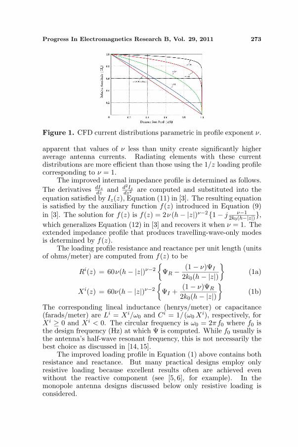
The generalized CFD current distribution is assumed to be of theform Iz(z) = C(h−|z| ) ν exp (−jk0 |z| ) where C is a complex constantdetermined by the current at the feed point. Instead of the WK lineardecay, the current amplitude now decays with a power law variation(h−|z| ) ν with exponent ν (profile exponent). As in [3], exp (−jk0 |z| )is the travelling wave propagation factor. When ν = 1 the Wu and Kingcase is recovered, but when ν 6= 1 the more general case is obtained.Figure 1 shows typical current amplitude distributions parametric inthe profile exponent ν, I0 being the CFD’s feed point current. It is


Figure 1. CFD current distributions parametric in profile exponent ν.

apparent that values of ν less than unity create significantly higheraverage antenna currents. Radiating elements with these currentdistributions are more efficient than those using the 1/z loading profilecorresponding to ν = 1.

The improved internal impedance profile is determined as follows.The derivatives dIz

dz and d2Izdz2 are computed and substituted into the

equation satisfied by Iz(z), Equation (11) in [3]. The resulting equationis satisfied by the auxiliary function f(z) introduced in Equation (9)in [3]. The solution for f(z) is f(z) = 2ν (h− |z|)ν−21− j ν−1

2k0(h−|z|),which generalizes Equation (12) in [3] and recovers it when ν = 1. Theextended impedance profile that produces travelling-wave-only modesis determined by f(z).

The loading profile resistance and reactance per unit length (unitsof ohms/meter) are computed from f(z) to be

Ri(z) = 60ν(h− |z|)ν−2

ΨR − (1− ν)ΨI

2k0(h− |z|)

(1a)

Xi(z) = 60ν(h− |z|)ν−2

ΨI +

(1− ν)ΨR

2k0(h− |z|)

(1b)

The corresponding lineal inductance (henrys/meter) or capacitance(farads/meter) are Li = Xi/ω0 and Ci = 1/(ω0 Xi), respectively, forXi ≥ 0 and Xi < 0. The circular frequency is ω0 = 2πf0 where f0 isthe design frequency (Hz) at which Ψ is computed. While f0 usually isthe antenna’s half-wave resonant frequency, this is not necessarily thebest choice as discussed in [14, 15].

The improved loading profile in Equation (1) above contains bothresistance and reactance. But many practical designs employ onlyresistive loading because excellent results often are achieved evenwithout the reactive component (see [5, 6], for example). In themonopole antenna designs discussed below only resistive loading isconsidered.

274 Formato

4. LOADED HF MONOPOLE USING ANALYTICPROFILE

Rama Rao and Debroux’s work provides a useful analytical andexperimental benchmark for testing the improved loading profile. Theydesigned, fabricated and measured a 35-foot tall, 2-inch diameter,continuously resistively loaded base-fed monopole antenna using fulland fractional WK profiles. The loading profile was computed usingWK theory and the antenna performance modeled with the NECMethod of Moments code version 3 (see below). The antenna then wasbuilt using different loading profiles, and extensive measurements weremade of its performance [5, 6]. The measured RD data validated boththe WK model and NEC’s results, to quote, “The input impedancevalues predicted by both theories are in good qualitative agreementwith the measured results and confirm the non-resonant behavior ofthe antenna.” [5, p. 1226].

NEC-modeled monopole performance thus agrees well withmeasured data, thereby validating NEC as an accurate predictive toolfor loaded wire element antenna design. The results reported here alsoare computed using NEC; but, instead of the RD loading profiles, newprofiles are applied using the extended WK theory and a numericaloptimization algorithm. This paper therefore compares its analyticalresults directly to RD’s analytical results through the NEC modelingengine. This paper does not, however, report new measurement resultsusing the modified loading profiles because, based on how well theRD measured and NEC-computed data agree, there is no reason evento suspect that NEC does not accurately calculate the monopole’sperformance.

The objectives of the RD design were (1) as flat as possiblean impedance bandwidth and (2) a stable radiation pattern at lowtake-off angles to support long range HF links from 5 to 30 MHz.A continuously varying resistance along the antenna was created bycoating a dielectric substrate with variable thickness chromium film.The RD design resulted in a voltage standing wave ratio (VSWR)≤ 2 : 1 relative to 50 Ω and radiation efficiency in the range 15%–36%. Because VSWR fluctuated substantially, achieving the VSWRobjective required the use of a 6-element matching network and 4 : 1transformer, a tradeoff that appears to be typical. As the impedanceresponse is progressively flattened in a loaded antenna, the radiationefficiency drops, often precipitously, and vice versa. The improvedloading profile described here mitigates this effect.

Equation (1) above was used to compute a discrete resistance-only loading profile for the RD monopole geometry, that is, a base-


fed element h = 10.668 meters tall, a = 0.0254 meters radius on aPEC (perfectly electrically conducting) ground plane. Because single-element lumped resistances are used, a filamentary antenna wire couldbe used instead of the 2-inch diameter substrate. But the samegeometry as the RD monopole was modeled because the antenna’slength-to-diameter ratio does influence its bandwidth, although in thiscase the effect is minor (a maximum bandwidth metallic monopoleelement has h ∼ 10a [16]).

The fundamental half-wave resonance of 7.028 MHz was usedas the design frequency. The generalized sine/cosine integralswere numerically evaluated using 32-point Gauss quadrature (seegenerally [13]). The antenna was modeled with NEC-2D (NumericalElectromagnetics Code Version 2 Double Precision), which was usedbecause it is freely available online [17]. NEC’s modeling guidelinesand the model validation procedure described in [18, 19] were followed,and as a check the antenna was modeled with the most recent versionof NEC as well (NEC-4.1D). Both versions of NEC yield essentiallythe same results.

Fourteen equal-length segments were used with each segmentloaded at its midpoint using NEC “LD” cards. The loading resistancevalue was calculated segment-by-segment as Rk

L = Ri(zck) · ∆, k =

1, . . . , 14 where ∆ = h/14 is the constant segment length and zck =

(2k − 1)∆2 is the z coordinate at the center of the kth segment. A

typical NEC input file appears in Figure 2.Runs were made using the profile exponent values in Figure 1,

and the corresponding loading profiles are plotted in Figure 3. Theheaviest loading is the full WK profile corresponding to ν = 1. Theresistor in the first segment has a value of 45.2 Ω, while the last segmentat the top of the monopole is loaded with 1220 Ω. Correspondingvalues for the least heavily loaded profile, ν = 0.05, are 0.27Ω and461.4Ω Interestingly, the loading resistance increases with increasingprofile exponent at all segments except the last where the three highestresistances in increasing order correspond to ν values of 1, 0.8, and0.4. But for all values of ν the data reflect the typical characteristic ofprogressively increasing resistance with distance from the RF sourceas seen in [1, 3–8]. As will be seen below, however, monotonicallyincreasing profiles are not necessarily the best.

Figures 4 and 5 plot the monopole’s input resistance andreactance. As for all plots in this paper, calculated data points aremarked by symbols, and the continuous curves connecting data pointshave been interpolated using a natural cubic spline. As expected,excursions in the antenna’s input impedance increase with decreasingprofile exponent. The most heavily loaded profiles, ν = 1 , 0.8,

276 Formato

Figure 2. Extended loading profile NEC input file for ν = 0.4.

Figure 3. Discrete extendedtheory loading profiles.

Figure 4. Loaded monopoleinput resistance.

show the flattest responses, especially for the input resistance. Forcomparison, the input impedance of the antenna with no loading(“metallic” monopole, ν = 0) is plotted as well, and, of course, itexhibits the greatest variability.

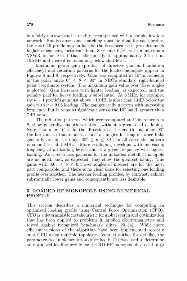
Radiation efficiency appears in Figure 6. The effect of the profileexponent is dramatic. At 5MHz, for example, the heavily loaded WKprofile with ν = 1 results in an efficiency of less than 4%, while thevery light loading profile ν = 0.05 increases it to nearly 70%. As with


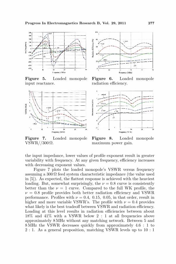
Figure 5. Loaded monopoleinput reactance.

Figure 6. Loaded monopoleradiation efficiency.

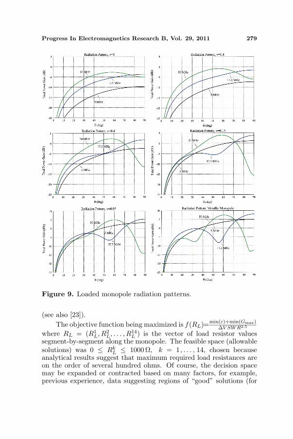
Figure 7. Loaded monopoleVSWR//300Ω.

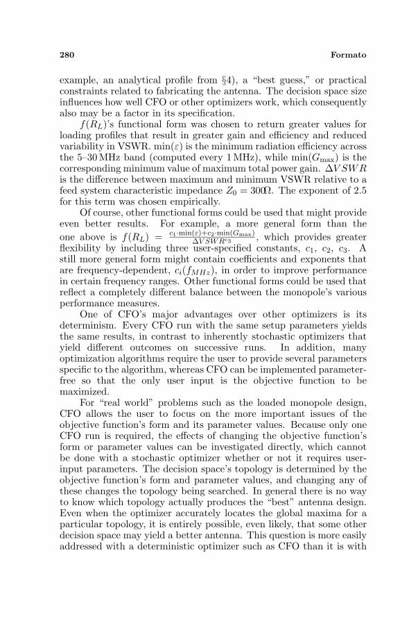
Figure 8. Loaded monopolemaximum power gain.

the input impedance, lower values of profile exponent result in greatervariability with frequency. At any given frequency, efficiency increaseswith decreasing exponent values.

Figure 7 plots the loaded monopole’s VSWR versus frequencyassuming a 300 Ω feed system characteristic impedance (the value usedin [5]). As expected, the flattest response is achieved with the heaviestloading. But, somewhat surprisingly, the ν = 0.8 curve is consistentlybetter than the ν = 1 curve. Compared to the full WK profile, theν = 0.8 profile provides both better radiation efficiency and VSWRperformance. Profiles with ν = 0.4, 0.15, 0.05, in that order, result inhigher and more variable VSWR’s. The profile with ν = 0.4 provideswhat likely is the best tradeoff between VSWR and radiation efficiency.Loading at this level results in radiation efficiencies between about18% and 41% with a VSWR below 2 : 1 at all frequencies aboveapproximately 8 MHz without any matching network. Between 5 and8MHz the VSWR decreases quickly from approximately 4.6 : 1 to2 : 1. As a general proposition, matching VSWR levels up to 10 : 1

278 Formato

in a fairly narrow band is readily accomplished with a simple, low-lossnetwork. But because some matching must be done for each profile,the ν = 0.15 profile may in fact be the best because it provides muchhigher efficiencies, between about 39% and 62%, with a maximumVSWR below 10 : 1 that falls quickly to approximately 2.5 : 1 at10MHz and thereafter remaining below that level.

Maximum power gain (product of directive gain and radiationefficiency) and radiation patterns for the loaded monopole appear inFigures 8 and 9, respectively. Gain was computed at 10 incrementsin the polar angle 0 ≤ θ ≤ 90 in NEC’s standard right-handedpolar coordinate system. The maximum gain value over these anglesis plotted. Gain increases with lighter loading, as expected, and thepenalty paid for heavy loading is substantial. At 5 MHz, for example,the ν = 1 profile’s gain just above−10 dBi is more than 13 dB below thegain with ν = 0.05 loading. The gap generally narrows with increasingfrequency, but it remains significant across the HF band, greater than7 dB or so.

The radiation patterns, which were computed at 1 increments inθ, show generally smooth variations without a great deal of lobing.Note that θ = 0 is in the direction of the zenith and θ = 90the horizon, so that moderate take-off angles for long-distance linksgenerally are in the range 60 ≤ θ ≤ 80. In all cases the patternis smoothest at 5 MHz. More scalloping develops with increasingfrequency at all loading levels, and at a given frequency with lighterloading. As a reference, patterns for the unloaded metallic monopoleare included, and, as expected, they show the greatest lobing. Thegains with 0.05 ≤ ν ≤ 0.4 over angles of interest are for the mostpart comparable, and there is no clear basis for selecting one loadingprofile over another. The heavier loading profiles, by contrast, exhibitsubstantially lower gains and consequently are less desirable.

5. LOADED HF MONOPOLE USING NUMERICALPROFILE

This section describes a numerical technique for computing anoptimized loading profile using Central Force Optimization (CFO).CFO is a deterministic metaheuristic for global search and optimizationthat has been applied to problems in applied electromagnetics andtested against recognized benchmark suites [20–34]. While moreefficient versions of the algorithm have been implemented recentlyon a GPU using multiple topologies (contact author for details), theparameter-free implementation described in [20] was used to determinean optimized loading profile for the RD HF monopole discussed in §4


Figure 9. Loaded monopole radiation patterns.

(see also [23]).The objective function being maximized is f(RL)=min(ε)+min(Gmax)

∆V SWR2.5

where RL = (R1L, R2

L, . . . , R14L ) is the vector of load resistor values

segment-by-segment along the monopole. The feasible space (allowablesolutions) was 0 ≤ Rk

L ≤ 1000Ω, k = 1 , . . . , 14, chosen becauseanalytical results suggest that maximum required load resistances areon the order of several hundred ohms. Of course, the decision spacemay be expanded or contracted based on many factors, for example,previous experience, data suggesting regions of “good” solutions (for

280 Formato

example, an analytical profile from §4), a “best guess,” or practicalconstraints related to fabricating the antenna. The decision space sizeinfluences how well CFO or other optimizers work, which consequentlyalso may be a factor in its specification.

f(RL)’s functional form was chosen to return greater values forloading profiles that result in greater gain and efficiency and reducedvariability in VSWR. min(ε) is the minimum radiation efficiency acrossthe 5–30 MHz band (computed every 1 MHz), while min(Gmax) is thecorresponding minimum value of maximum total power gain. ∆V SWRis the difference between maximum and minimum VSWR relative to afeed system characteristic impedance Z0 = 300Ω. The exponent of 2.5for this term was chosen empirically.

Of course, other functional forms could be used that might provideeven better results. For example, a more general form than theone above is f(RL) = c1·min(ε)+c2·min(Gmax)

∆V SWRc3 , which provides greaterflexibility by including three user-specified constants, c1, c2, c3. Astill more general form might contain coefficients and exponents thatare frequency-dependent, ci(fMHz), in order to improve performancein certain frequency ranges. Other functional forms could be used thatreflect a completely different balance between the monopole’s variousperformance measures.

One of CFO’s major advantages over other optimizers is itsdeterminism. Every CFO run with the same setup parameters yieldsthe same results, in contrast to inherently stochastic optimizers thatyield different outcomes on successive runs. In addition, manyoptimization algorithms require the user to provide several parametersspecific to the algorithm, whereas CFO can be implemented parameter-free so that the only user input is the objective function to bemaximized.

For “real world” problems such as the loaded monopole design,CFO allows the user to focus on the more important issues of theobjective function’s form and its parameter values. Because only oneCFO run is required, the effects of changing the objective function’sform or parameter values can be investigated directly, which cannotbe done with a stochastic optimizer whether or not it requires user-input parameters. The decision space’s topology is determined by theobjective function’s form and parameter values, and changing any ofthese changes the topology being searched. In general there is no wayto know which topology actually produces the “best” antenna design.Even when the optimizer accurately locates the global maxima for aparticular topology, it is entirely possible, even likely, that some otherdecision space may yield a better antenna. This question is more easilyaddressed with a deterministic optimizer such as CFO than it is with


a stochastic optimizer whose results never are the same.The CFO optimization run reported here employs the parameter-

free implementation described in [20] with directional informationincluded in errant probe repositioning described in [31] and thefollowing hard-wired parameter values: F init

rep = 0.5, ∆Frep = 0.1,γstart = 0, γstop = 1, ∆γ = 0.1, Nd = 14, (Np/Nd)max = 4, Nt = 120.Pseudocode appears in Figure 10. Readers wishing to implement theirown versions of the program are advised to consult [20] for additionalinformation that is beyond the scope of this paper.

Evolution of the optimizer’s best fitness (objective function value),average probe distance (Davg), and CFO’s best probe number are

[20]

[20]

[20]

[31]

(see [27,29]):

[31]

[20]

[20]

Figure 10. Parameter-free CFO Pseudocode (Ω is the decision space).

282 Formato

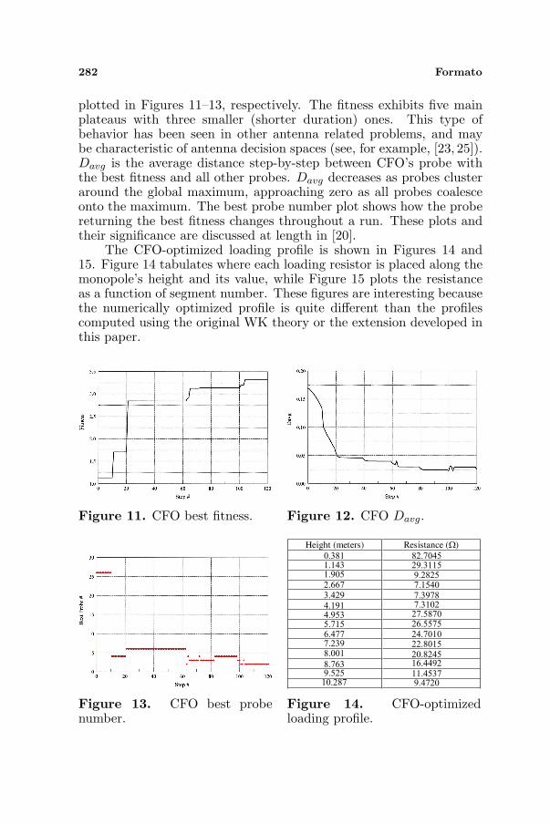
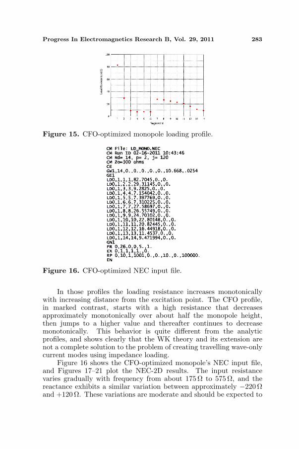
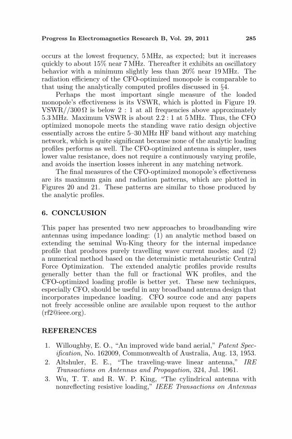
plotted in Figures 11–13, respectively. The fitness exhibits five mainplateaus with three smaller (shorter duration) ones. This type ofbehavior has been seen in other antenna related problems, and maybe characteristic of antenna decision spaces (see, for example, [23, 25]).Davg is the average distance step-by-step between CFO’s probe withthe best fitness and all other probes. Davg decreases as probes clusteraround the global maximum, approaching zero as all probes coalesceonto the maximum. The best probe number plot shows how the probereturning the best fitness changes throughout a run. These plots andtheir significance are discussed at length in [20].

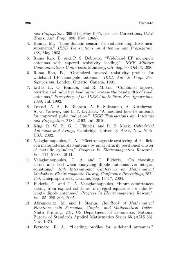
The CFO-optimized loading profile is shown in Figures 14 and15. Figure 14 tabulates where each loading resistor is placed along themonopole’s height and its value, while Figure 15 plots the resistanceas a function of segment number. These figures are interesting becausethe numerically optimized profile is quite different than the profilescomputed using the original WK theory or the extension developed inthis paper.

Figure 11. CFO best fitness. Figure 12. CFO Davg.

Figure 13. CFO best probenumber.

Height (meters) Resistance (Ω )

0.381 82.7045

1.143

1.905

2.667

3.429

4.191

4.953

5.715

6.477

7.239

8.001

8.763

9.525

10.287

29.3115

9.2825

7.1540

7.3978

7.3102

27.5870

26.5575

24.7010

22.8015

20.8245

16.4492

11.4537

9.4720

Figure 14. CFO-optimizedloading profile.


Figure 15. CFO-optimized monopole loading profile.

Figure 16. CFO-optimized NEC input file.

In those profiles the loading resistance increases monotonicallywith increasing distance from the excitation point. The CFO profile,in marked contrast, starts with a high resistance that decreasesapproximately monotonically over about half the monopole height,then jumps to a higher value and thereafter continues to decreasemonotonically. This behavior is quite different from the analyticprofiles, and shows clearly that the WK theory and its extension arenot a complete solution to the problem of creating travelling wave-onlycurrent modes using impedance loading.

Figure 16 shows the CFO-optimized monopole’s NEC input file,and Figures 17–21 plot the NEC-2D results. The input resistancevaries gradually with frequency from about 175 Ω to 575 Ω, and thereactance exhibits a similar variation between approximately −220Ωand +120Ω. These variations are moderate and should be expected to

284 Formato

Figure 17. CFO loadedmonopole input impedance.

Figure 18. CFO loadedmonopole radiation efficiency.

Figure 19. CFO LoadedMonopole VSWR//300 Ω.

Figure 20. CFO loadedmonopole maximum gain.

Figure 21. CFO loaded monopole radiation pattern.

result in a similarly moderate VSWR variation. Four resonant points(Xin = 0) appear below approximately 7.5, 15, 21 and 27.5 MHz atalternate resonances and anti-resonances in the monopole structure.

Figure 18 plots the monopole’s radiation efficiency which rangesfrom a low of about 9% to a maximum of 45%. The worst efficiency


occurs at the lowest frequency, 5 MHz, as expected; but it increasesquickly to about 15% near 7 MHz. Thereafter it exhibits an oscillatorybehavior with a minimum slightly less than 20% near 19 MHz. Theradiation efficiency of the CFO-optimized monopole is comparable tothat using the analytically computed profiles discussed in §4.

Perhaps the most important single measure of the loadedmonopole’s effectiveness is its VSWR, which is plotted in Figure 19.VSWR//300Ω is below 2 : 1 at all frequencies above approximately5.3MHz. Maximum VSWR is about 2.2 : 1 at 5 MHz. Thus, the CFOoptimized monopole meets the standing wave ratio design objectiveessentially across the entire 5–30MHz HF band without any matchingnetwork, which is quite significant because none of the analytic loadingprofiles performs as well. The CFO-optimized antenna is simpler, useslower value resistance, does not require a continuously varying profile,and avoids the insertion losses inherent in any matching network.

The final measures of the CFO-optimized monopole’s effectivenessare its maximum gain and radiation patterns, which are plotted inFigures 20 and 21. These patterns are similar to those produced bythe analytic profiles.

6. CONCLUSION

This paper has presented two new approaches to broadbanding wireantennas using impedance loading: (1) an analytic method based onextending the seminal Wu-King theory for the internal impedanceprofile that produces purely travelling wave current modes; and (2)a numerical method based on the deterministic metaheuristic CentralForce Optimization. The extended analytic profiles provide resultsgenerally better than the full or fractional WK profiles, and theCFO-optimized loading profile is better yet. These new techniques,especially CFO, should be useful in any broadband antenna design thatincorporates impedance loading. CFO source code and any papersnot freely accessible online are available upon request to the author([email protected]).

REFERENCES

1. Willoughby, E. O., “An improved wide band aerial,” Patent Spec-ification, No. 162009, Commonwealth of Australia, Aug. 13, 1953.

2. Altshuler, E. E., “The traveling-wave linear antenna,” IRETransactions on Antennas and Propagation, 324, Jul. 1961.

3. Wu, T. T. and R. W. P. King, “The cylindrical antenna withnonreflecting resistive loading,” IEEE Transactions on Antennas

286 Formato

and Propagation, 369–373, May 1965, (see also Corrections, IEEETrans. Ant. Prop., 998, Nov. 1965).

4. Kanda, M., “Time domain sensors for radiated impulsive mea-surements,” IEEE Transactions on Antennas and Propagation,438, May 1983.

5. Rama Rao, B. and P. S. Debroux, “Wideband HF monopoleantennas with tapered resistivity loading,” IEEE MilitaryCommunications Conference, Monterey, CA, Sep. 30–Oct. 3, 1990.

6. Rama Rao, B., “Optimized tapered resistivity profiles forwideband HF monopole antenna,” IEEE Ant. & Prop. Soc.Symposium, London, Ontario, Canada, 1991.

7. Little, L., O. Ramabi, and R. Mittra, “Combined taperedresistive and inductive loading to increase the bandwidth of smallantennas,” Proceedings of the IEEE Ant. & Prop. Soc. Symposium,2089, Jul. 1992.

8. Lestari, A. A., E. Bharata, A. B. Suksmono, A. Kurniawan,A. G. Yarovoy, and L. P. Ligthart, “A modified bow-tie antennafor improved pulse radiation,” IEEE Transactions on Antennasand Propagation, 2184–2192, Jul. 2010.

9. King, R. W. P., G. J. Fikioris, and R. B. Mack, CylindricalAntennas and Arrays, Cambridge University Press, New York,USA, 2002.

10. Valagiannopoulos, C. A., “Electromagnetic scattering of the fieldof a metamaterial slab antenna by an arbitrarily positioned clusterof metallic cylinders,” Progress In Electromagnetics Research,Vol. 114, 51–66, 2011.

11. Valagiannopoulos, C. A. and G. Fikioris, “On choosingkernel and feed when analyzing dipole antennas via integralequations,” 10th International Conference on MathematicalMethods in Electromagnetic Theory, Conference Proceedings, 257–259, Dniepropetrovsk, Ukraine, Sep. 14–17, 2004.

12. Fikioris, G. and C. A. Valagiannopoulos, “Input admittancesarising from explicit solutions to integral equations for infinite-length dipole antennas,” Progress In Electromagnetics Research,Vol. 55, 285–306, 2005.

13. Abramowitz, M. and I. Stegun, Handbook of MathematicalFunctions with Formulas, Graphs, and Mathematical Tables,Ninth Printing, 231, US Department of Commerce, NationalBureau of Standards Applied Mathematics Series 55 (AMS 55),Nov. 1970.

14. Formato, R. A., “Loading profiles for wideband antennas,”


Communications Quarterly Magazine, 27, Summer 1997, (see alsoCorrections, 93, Fall 1997).

15. Formato, R. A., “Wideband antennas,” Electronics WorldMagazine, 202, Mar. 1997.

16. Formato, R. A., “Maximizing the bandwidth of monopoleantennas,” NARTE News, Vol. 11, No. 4, 5, National Associationof Radio and Telecommunications Engineers, Inc., Oct. 1993–Jan. 1994.

17. (i) 4nec2 Antenna Modeling Freeware by A. Voors, availableonline at http://home.ict.nl/∼arivoors/. (ii) Unofficial NumericalElectromagnetic Code (NEC) Archives, online at http://www.si-list.net/swindex.html.

18. Burke, G. J. and A. J. Poggio, “Numerical electromagnetics code(NEC) — Method of moments,” Parts I, II and III, UCID-19934,Lawrence Livermore National Laboratory, Livermore, California,USA, Jan. 1981.

19. Burke, G. J., “Numerical electromagnetics code — NEC-4,method of moments, Part I: User’s manual and Part II: Programdescription — Theory,” UCRL-MA-109338, Lawrence LivermoreNational Laboratory, Livermore, California, USA, Jan. 1992,https://ipo.llnl.gov/technology/software/softwaretitles/nec.php.

20. Formato, R. A., “Parameter-free deterministic global searchwith simplified central force optimization,” Proceeding ICIC’10Proceedings of the 6th International Conference on AdvancedIntelligent Computing Theories and Applications: IntelligentComputing , 309–318, Springer-Verlag, Berlin, Heidelberg, 2010.

21. Cross, M. W., E. Merulla, and R. A. Formato, “High-performance indoor VHF-UHF antennas: Technology updatereport,” National Association of Broadcasters (NAB), FAS-TROAD (Flexible Advanced Services for Television and RadioOn All Devices), Technology Advocacy Program, May 15, 2010,http://www.nabfastroad.org/NABHighperformanceIndoorTVantennaRpt.pdf.

22. Qubati, G. M., N. I. Dib, and R. A. Formato, “Antennabenchmark performance and array synthesis using central forceoptimization,” IET (UK) Microwaves, Antennas & Propagation,Vol. 4, No. 5, 583–592, 2010, doi: 10.1049/iet-map.2009.0147.

23. Formato, R. A., “Improved CFO algorithm for antenna opti-mization,” Progress In Electromagnetics Research B, 405–425,2010, http://www.jpier.org/pierb/pier.php?paper=09112309,doi:10.2528/PIERB09112309.

24. Formato, R. A., “Central force optimization and NEOs — First

288 Formato

cousins?,” Journal of Multiple-valued Logic and Soft Computing,Vol. 16, 547–565, 2010.

25. Formato, R. A., “Central force optimization applied to thePBM suite of antenna benchmarks,” 2010, arXiv:1003.0221,http://arXiv.org.

26. Xie, L., J. Zeng, and R. A. Formato, “Convergence analysisand performance of the extended artificial physics optimizationalgorithm,” Applied Mathematics and Computation, 2011, onlineat http://dx.doi.org/10.1016/j.amc.2011.02.062.

27. Formato, R. A., “Central force optimisation: A new gradient-likemetaheuristic for multidimensional search and optimisation,” Int.J. Bio-inspired Computation, Vol. 1, No. 4, 217–238, 2009, doi:10.1504/IJBIC.2009.024721.

28. Formato, R. A., “Central force optimization: A new deterministicgradient-like optimization metaheuristic,” Journal of the Opera-tions Research Society of India, Vol. 46, No. 1, 25–51, 2009, doi:10.1007/s12597-009-0003-4.

29. Formato, R. A., “Central force optimization: A new computa-tional framework for multidimensional search and optimization,”Nature Inspired Cooperative Strategies for Optimization (NICSO2007), N. Krasnogor, G. Nicosia, M. Pavone, and D. Pelta, Eds.,Vol. 129, Springer-Verlag, Heidelberg, 2008.

30. Formato, R. A., “Central force optimization: A new metaheuristicwith applications in applied electromagnetics,” Progress InElectromagnetics Research, Vol. 77, 425–491, 2007.

31. Formato, R. A., “On the utility of directional information forrepositioning errant probes in central force optimization,” 2010,arXiv:1005.5490, http://arXiv.org.

32. Formato, R. A., “Pseudorandomness in central force optimiza-tion,” 2010, arXiv:1001.0317, http://arXiv.org.

33. Formato, R. A., “Are near earth objects the key to optimizationtheory?” 2009, arXiv:0912.1394, http://arXiv.org.

34. Formato, R. A., “Issues in antenna optimization — A monopolecase study,” Mar. 2011, http://arXiv.org/abs/1103.5629.

new techniques for increasing antenna … · of wire antennas using impedance loading. this paper...

Documents