new support vector algorithms - purdue universityyuzhu/stat598m3/papers/newsv… · ·...

LETTER Communicated by John Platt

New Support Vector Algorithms

Bernhard Scholkopf curren

Alex J SmolaGMD FIRST 12489 Berlin Germany and Department of Engineering AustralianNational University Canberra 0200 Australia

Robert C WilliamsonDepartment of Engineering Australian National UniversityCanberra 0200Australia

Peter L BartlettRSISE Australian National University Canberra 0200 Australia

We propose a new class of support vector algorithms for regression andclassication In these algorithms a parameter ordm lets one effectively con-trol the number of support vectors While this can be useful in its ownright the parameterization has the additional benet of enabling us toeliminate one of the other free parameters of the algorithm the accuracyparameter e in the regression case and the regularization constant C in theclassication case We describe the algorithms give some theoretical re-sults concerning the meaning and the choice ofordm and report experimentalresults

1 Introduction

Support vector (SV) machines comprise a new class of learning algorithmsmotivated by results of statistical learning theory (Vapnik 1995) Originallydeveloped for pattern recognition (Vapnik amp Chervonenkis 1974 BoserGuyon amp Vapnik 1992) they represent the decision boundary in terms ofa typically small subset (Scholkopf Burges amp Vapnik 1995) of all trainingexamples called the support vectors In order for this sparseness propertyto carry over to the case of SV Regression Vapnik devised the so-callede-insensitive loss function

|y iexcl f (x)|e Dmaxf0 |y iexcl f (x)| iexcl eg (11)

which does not penalize errors below some e gt 0 chosen a priori Hisalgorithm which we will henceforth call e-SVR seeks to estimate functions

f (x) D (w cent x) C b w x 2 RN b 2 R (12)

curren Present address Microsoft Research 1 Guildhall Street Cambridge UK

Neural Computation 12 1207ndash1245 (2000) cdeg 2000 Massachusetts Institute of Technology

1208 B Scholkopf A J Smola R C Williamson and P L Bartlett

based on independent and identically distributed (iid) data

(x1 y1) (x` y ) 2 RN pound R (13)

Here RN is the space in which the input patterns live but most of the fol-lowing also applies for inputs from a set X The goal of the learning processis to nd a function f with a small risk (or test error)

R[ f ] DZ

l( f x y) dP(x y) (14)

where P is the probability measure which is assumed to be responsible forthe generation of the observations (see equation 13) and l is a loss func-tion for example l( f x y) D ( f (x) iexcl y)2 or many other choices (Smola ampScholkopf 1998) The particular loss function for which we would like tominimize equation 14 depends on the specic regression estimation prob-lem at hand This does not necessarily have to coincide with the loss functionused in our learning algorithm First there might be additional constraintsthat we would like our regression estimation to satisfy for instance that ithave a sparse representation in terms of the training data In the SVcase thisis achieved through the insensitive zone in equation 11 Second we cannotminimize equation 14 directly in the rst place since we do not know PInstead we are given the sample equation 13 and we try to obtain a smallrisk by minimizing the regularized risk functional

12

kwk2 C C cent Reemp[ f ] (15)

Here kwk2 is a term that characterizes the model complexity

Reemp[ f ] D

1`

X

iD1

|yi iexcl f (xi)|e (16)

measures the e-insensitive training error and C is a constant determiningthe trade-off In short minimizing equation 15 captures the main insightof statistical learning theory stating that in order to obtain a small risk oneneeds to control both training error and model complexitymdashthat is explainthe data with a simple model

The minimization of equation 15 is equivalent to the following con-strained optimization problem (see Figure 1)

minimize t (w raquo(curren)) D 12

kwk2 C C cent 1`

X

iD1

(ji C j curreni ) (17)

New Support Vector Algorithms 1209

Figure 1 In SV regression a desired accuracy e is specied a priori It is thenattempted to t a tube with radius e to the data The trade-off between modelcomplexity and points lying outside the tube (with positive slack variablesj ) isdetermined by minimizing the expression 15

subject to ((w cent xi) C b) iexcl yi middot e C ji (18)

yi iexcl ((w cent xi) C b) middot e C j curreni (19)

j(curren)i cedil 0 (110)

Here and below it is understood that i D1 and that boldface Greekletters denote -dimensional vectors of the corresponding variables (curren) is ashorthand implying both the variables with and without asterisks

By using Lagrange multiplier techniques one can show (Vapnik 1995)that this leads to the following dual optimization problem Maximize

W(reg regcurren) D iexcleX

iD1

(acurreni C ai) C

X

iD1

(acurreni iexcl ai)yi

iexcl 12

X

i jD1

(acurreni iexcl ai)(acurren

j iexcl aj)(xi cent xj) (111)

subject toX

iD1

(ai iexcl acurreni ) D0 (112)

a(curren)i 2

h0 C

`

i (113)

The resulting regression estimates are linear however the setting can begeneralized to a nonlinear one by using the kernel method As we will useprecisely this method in the next section we shall omit its exposition at thispoint


To motivate the new algorithm that we shall propose note that the pa-rameter e can be useful if the desired accuracy of the approximation can bespecied beforehand In some cases however we want the estimate to be asaccurate as possible without having to commit ourselves to a specic levelof accuracy a priori In this work we rst describe a modication of the e-SVR algorithm called ordm-SVR which automatically minimizes e Followingthis we present two theoretical results onordm-SVR concerning the connectionto robust estimators (section 3) and the asymptotically optimal choice of theparameter ordm (section 4) Next we extend the algorithm to handle parametricinsensitivity models that allow taking into account prior knowledge aboutheteroscedasticity of the noise As a bridge connecting this rst theoreti-cal part of the article to the second one we then present a denition of amargin that both SV classication and SV regression algorithms maximize(section 6) In view of this close connection between both algorithms it isnot surprising that it is possible to formulate also a ordm-SV classication al-gorithm This is done including some theoretical analysis in section 7 Weconclude with experiments and a discussion

2 ordm-SV Regression

To estimate functions (see equation 12) from empirical data (see equa-tion 13) we proceed as follows (Scholkopf Bartlett Smola amp Williamson1998) At each point xi we allow an error of e Everything above e is cap-tured in slack variables j

(curren)i which are penalized in the objective function

via a regularization constant C chosen a priori (Vapnik 1995) The size ofe is traded off against model complexity and slack variables via a constantordm cedil 0

minimize t (w raquo(curren) e) D

12

kwk2 C C cent (ordme C1`

X

iD1

(ji C j curreni )

(21)



j(curren)i cedil 0 e cedil 0 (24)

For the constraints we introduce multipliers a(curren)i g(curren)

i b cedil 0 and obtain theLagrangian

L(w b reg(curren) b raquo(curren) e acute(curren))

D 12

kwk2 C Cordme CC`

X

iD1

(ji C j curreni ) iexcl be iexcl

X

iD1

(giji C gcurreni j

curreni )


iexclX

iD1

ai(ji C yi iexcl (w cent xi) iexcl b C e)

iexclX

iD1

acurreni (j curren

i C (w cent xi) C b iexcl yi C e) (25)

To minimize the expression 21 we have to nd the saddle point of Lmdashthatis minimize over the primal variables w e bj (curren)

i and maximize over thedual variables a

(curren)i bg(curren)

i Setting the derivatives with respect to the primalvariables equal to zero yields four equations

w DX

i(acurren

i iexcl ai)xi (26)

C centordm iexclX

i(ai C acurren

i ) iexcl b D0 (27)

X

iD1


C`

iexcl a(curren)i iexcl g

(curren)i D0 (29)

In the SV expansion equation 26 only those a(curren)i will be nonzero that cor-

respond to a constraint equations 22 or 23 which is precisely met thecorrespondingpatterns are called support vectors This is due to the Karush-Kuhn-Tucker (KKT) conditions that apply to convex constrained optimiza-tion problems (Bertsekas 1995) If we write the constraints as g(xi yi) cedil0 with corresponding Lagrange multipliers ai then the solution satisesai cent g(xi yi) D0 for all i

Substituting the above four conditions into L leads to another optimiza-tion problem called the Wolfe dual Before stating it explicitly we carryout one further modication Following Boser et al (1992) we substitute akernel k for the dot product corresponding to a dot product in some featurespace related to input space via a nonlinear map W

k(x y) D (W(x) cent W(y)) (210)

By using k we implicitly carry out all computations in the feature space thatW maps into which can have a very high dimensionality The feature spacehas the structure of a reproducing kernel Hilbert space (Wahba 1999 Girosi1998 Scholkopf 1997) and hence minimization of kwk2 can be understood inthe context of regularization operators (Smola Scholkopf amp Muller 1998)

The method is applicable whenever an algorithm can be cast in terms ofdot products (Aizerman Braverman amp Rozonoer 1964 Boser et al 1992Scholkopf Smola amp Muller 1998) The choice of k is a research topic in its


own right that we shall not touch here (Williamson Smola amp Scholkopf1998 Scholkopf Shawe-Taylor Smola amp Williamson 1999) typical choicesinclude gaussian kernels k(x y) D exp(iexclkx iexcl yk2 (2s2)) and polynomialkernels k(x y) D (x cent y)d (s gt 0 d 2 N)

Rewriting the constraints noting that b g(curren)i cedil 0 do not appear in the

dual we arrive at the ordm-SVR optimization problem for ordm cedil 0 C gt 0

maximize W(reg(curren)) DX

iD1


iexcl 12

X

i jD1


j iexcl aj)k(xi xj) (211)

subject toX

iD1


a(curren)i 2

h0 C

`

i(213)

X

iD1

(ai C acurreni ) middot C centordm (214)

The regression estimate then takes the form (cf equations 12 26 and 210)

f (x) DX

iD1

(acurreni iexcl ai)k(xi x) C b (215)

where b (and e) can be computed by taking into account that equations 22and 23 (substitution of

Pj(a

currenj iexcl aj)k(xj x) for (w cent x) is understood cf

equations 26 and 210) become equalities with j(curren)i D 0 for points with

0 lt a(curren)i lt C respectively due to the KKT conditions

Before we give theoretical results explaining the signicance of the pa-rameter ordm the following observation concerning e is helpful If ordm gt 1 thene D 0 since it does not pay to increase e (cf equation 21) If ordm middot 1 it canstill happen that e D 0mdashfor example if the data are noise free and can beperfectly interpolated with a low-capacity model The case e D0 howeveris not what we are interested in it corresponds to plain L1-loss regression

We will use the term errors to refer to training points lying outside thetube1 and the term fraction of errors or SVs to denote the relative numbers of

1 For N gt 1 the ldquotuberdquo should actually be called a slabmdashthe region between twoparallel hyperplanes


errors or SVs (ie divided by ) In this proposition we dene the modulusof absolute continuity of a function f as the function 2 (d ) D sup

Pi | f (bi) iexcl

f (ai)| where the supremum is taken over all disjoint intervals (ai bi) withai lt bi satisfying

Pi(bi iexcl ai) lt d Loosely speaking the condition on the

conditional density of y given x asks that it be absolutely continuous ldquoonaveragerdquo

Proposition 1 Suppose ordm-SVR is applied to some data set and the resulting eis nonzero The following statements hold

i ordm is an upper bound on the fraction of errors

ii ordm is a lower bound on the fraction of SVs

iii Suppose the data (see equation 13) were generated iid from a distributionP(x y) D P(x)P(y|x) with P(y|x) continuous and the expectation of themodulus of absolute continuity of its density satisfying limd0 E2 (d ) D 0With probability 1 asymptotically ordm equals both the fraction of SVs and thefraction of errors

Proof Ad (i) The constraints equations 213 and 214 imply that at mosta fraction ordm of all examples can have a

(curren)i DC All examples with j

(curren)i gt 0

(ie those outside the tube) certainly satisfy a(curren)i D C ` (if not a

(curren)i could

grow further to reduce j(curren)i )

Ad (ii) By the KKT conditions e gt 0 implies b D0 Hence equation 214becomes an equality (cf equation 27)2 Since SVs are those examples forwhich 0 lt a

(curren)i middot C the result follows (using ai cent acurren

i D 0 for all i Vapnik1995)

Ad (iii) The strategy of proof is to show that asymptotically the proba-bility of a point is lying on the edge of the tube vanishes The condition onP(y|x) means that

supft

EPiexcl| f (x) C t iexcl y| lt c

shyshyxcent

lt d (c ) (216)

for some function d (c ) that approaches zero as c 0 Since the class ofSV regression estimates f has well-behaved covering numbers we have(Anthony amp Bartlett 1999 chap 21) that for all t

Pr (supf

sup3OP`(| f (x)C t iexcl y| lt c 2) lt P(| f (x)C tiexcly| lt c )

acutegt a

lt c1ciexcl`

2

2 In practice one can alternatively work with equation 214 as an equality constraint


where OP` is the sample-based estimate of P (that is the proportion of pointsthat satisfy | f (x)iexclyC t| lt c ) and c1 c2 may depend onc and a Discretizingthe values of t taking the union bound and applying equation 216 showsthat the supremum over f and t of OP`( f (x) iexcl y C t D0) converges to zero inprobability Thus the fraction of points on the edge of the tube almost surelyconverges to 0 Hence the fraction of SVs equals that of errors Combiningstatements i and ii then shows that both fractions converge almost surelyto ordm

Hence 0 middot ordm middot 1 can be used to control the number of errors (note that forordm cedil 1 equation 213 implies 214 since ai cent acurren

i D 0 for all i (Vapnik 1995))Moreover since the constraint equation 212 implies that equation 214 isequivalent to

Pi a

(curren)i middot Cordm2 we conclude that proposition 1 actually holds

for the upper and the lower edges of the tube separately with ordm2 each(Note that by the same argument the number of SVs at the two edges of thestandard e-SVR tube asymptotically agree)

A more intuitive albeit somewhat informal explanation can be givenin terms of the primal objective function (see equation 21) At the pointof the solution note that if e gt 0 we must have (e)t (w e) D 0 thatis ordm C (e)Re

emp D 0 hence ordm D iexcl(e)Reemp This is greater than or

equal to the fraction of errors since the points outside the tube certainlydo contribute to a change in Remp when e is changed Points at the edge ofthe tube possibly might also contribute This is where the inequality comesfrom

Note that this does not contradict our freedom to choose ordm gt 1 In thatcase e D0 since it does not pay to increase e (cf equation 21)

Let us briey discuss howordm-SVR relates to e-SVR (see section 1) Both al-gorithms use the e-insensitive loss function but ordm-SVR automatically com-putes e In a Bayesian perspective this automatic adaptation of the lossfunction could be interpreted as adapting the error model controlled by thehyperparameterordm Comparing equation 111 (substitution of a kernel for thedot product is understood) and equation 211 we note that e-SVR requiresan additional term iexcle

PìD1(acurren

i C ai) which for xed e gt 0 encouragesthat some of the a

(curren)i will turn out to be 0 Accordingly the constraint (see

equation 214) which appears inordm-SVR is not needed The primal problemsequations 17 and 21 differ in the term ordme If ordm D 0 then the optimizationcan grow e arbitrarily large hence zero empirical risk can be obtained evenwhen all as are zero

In the following sense ordm-SVR includes e-SVR Note that in the generalcase using kernels Nw is a vector in feature space

Proposition 2 If ordm-SVR leads to the solution Ne Nw Nb then e-SVR with e set apriori to Ne and the same value of C has the solution Nw Nb


Proof If we minimize equation 21 then x e and minimize only over theremaining variables The solution does not change

3 The Connection to Robust Estimators

Using the e-insensitive loss function only the patterns outside the e-tubeenter the empirical risk term whereas the patterns closest to the actualregression have zero loss This however does not mean that it is only theoutliers that determine the regression In fact the contrary is the case

Proposition 3 (resistance of SV regression) Using support vector regressionwith the e-insensitive loss function (see equation 11) local movements of targetvalues of points outside the tube do not inuence the regression

Proof Shifting yi locally does not change the status of (xi yi) as being apoint outside the tube Then the dual solution reg(curren) is still feasible it satisesthe constraints (the point still has a

(curren)i DC ) Moreover the primal solution

withji transformed according to the movement of yi is also feasible Finallythe KKT conditions are still satised as still a

(curren)i D C Thus (Bertsekas

1995) reg(curren) is still the optimal solution

The proof relies on the fact that everywhere outside the tube the upperbound on the a

(curren)i is the same This is precisely the case if the loss func-

tion increases linearly ouside the e-tube (cf Huber 1981 for requirementson robust cost functions) Inside we could use various functions with aderivative smaller than the one of the linear part

For the case of the e-insensitive loss proposition 3 implies that essentiallythe regression is a generalization of an estimator for the mean of a randomvariable that does the following

Throws away the largest and smallest examples (a fractionordm2 of eithercategory in section 2 it is shown that the sum constraint equation 212implies that proposition 1 can be applied separately for the two sidesusing ordm2)

Estimates the mean by taking the average of the two extremal ones ofthe remaining examples

This resistance concerning outliers is close in spirit to robust estima-tors like the trimmed mean In fact we could get closer to the idea of thetrimmed mean which rst throws away the largest and smallest pointsand then computes the mean of the remaining points by using a quadraticloss inside the e-tube This would leave us with Huberrsquos robust loss func-tion


Note moreover that the parameter ordm is related to the breakdown pointof the corresponding robust estimator (Huber 1981) Because it speciesthe fraction of points that may be arbitrarily bad outliers ordm is related to thefraction of some arbitrary distribution that may be added to a known noisemodel without the estimator failing

Finally we add that by a simple modication of the loss function (White1994)mdashweighting the slack variables raquo

(curren) above and below the tube in the tar-get function equation 21 by 2l and 2(1iexcll) withl 2 [0 1]mdashrespectivelymdashone can estimate generalized quantiles The argument proceeds as followsAsymptotically all patterns have multipliers at bound (cf proposition 1)Thel however changes the upper bounds in the box constraints applyingto the two different types of slack variables to 2Cl ` and 2C(1 iexcl l) re-spectively The equality constraint equation 28 then implies that (1 iexcl l)and l give the fractions of points (out of those which are outside the tube)that lie on the two sides of the tube respectively

4 Asymptotically Optimal Choice of ordm

Using an analysis employing tools of information geometry (MurataYoshizawa amp Amari 1994 Smola Murata Scholkopf amp Muller 1998) wecan derive the asymptotically optimal ordm for a given class of noise models inthe sense of maximizing the statistical efciency3

Remark Denote p a density with unit variance4 and P a family of noisemodels generated from P by P D fp|p D 1

sP( y

s) s gt 0g Moreover

assume that the data were generated iid from a distribution p(x y) Dp(x)p(y iexcl f (x)) with p(y iexcl f (x)) continuous Under the assumption that SVregression produces an estimate Of converging to the underlying functionaldependency f the asymptotically optimal ordm for the estimation-of-location-parameter model of SV regression described in Smola Murata Scholkopfamp Muller (1998) is

ordm D 1 iexclZ e

iexcleP(t) dt where

e D argmint

1(P(iexclt ) C P(t))2

iexcl1 iexcl

Z t

iexclt

P(t) dtcent

(41)

3 This section assumes familiarity with some concepts of information geometryA morecomplete explanation of the model underlying the argument is given in Smola MurataScholkopf amp Muller (1998) and can be downloaded from httpsvmrstgmdde

4 is a prototype generating the class of densities Normalization assumptions aremade for ease of notation


To see this note that under the assumptions stated above the probabilityof a deviation larger than e Prf|y iexcl Of (x)| gt eg will converge to

Prcopy|y iexcl f (x)| gt e

ordfD

Z

poundfRn[iexclee]gp(x)p(j ) dx dj

D 1 iexclZ e

iexclep(j ) dj (42)

This is also the fraction of samples that will (asymptotically) become SVs(proposition 1 iii) Therefore an algorithm generating a fraction ordm D 1 iexclR e

iexcle p(j ) dj SVs will correspond to an algorithm with a tube of size e Theconsequence is that given a noise model p(j ) one can compute the optimale for it and then by using equation 42 compute the corresponding optimalvalue ordm

To this end one exploits the linear scaling behavior between the standarddeviation s of a distribution p and the optimal e This result establishedin Smola Murata Scholkopf amp Muller (1998) and Smola (1998) cannot beproved here instead we shall merely try to give a avor of the argumentThe basic idea is to consider the estimation of a location parameter using thee-insensitive loss with the goal of maximizing the statistical efciency Us-ing the Cramer-Rao bound and a result of Murata et al (1994) the efciencyis found to be

esup3e

s

acuteD

Q2

GI (43)

Here I is the Fisher information while Q and G are information geometricalquantities computed from the loss function and the noise model

This means that one only has to consider distributions of unit variancesay P to compute an optimal value of ordm that holds for the whole class ofdistributions P Using equation 43 one arrives at

1e(e)

GQ2 D

1(P(iexcle) C P(e))2

iexcl1 iexcl

Z e

iexcleP(t) dt

cent (44)

The minimum of equation 44 yields the optimal choice of e which allowscomputation of the correspondingordm and thus leads to equation 41

Consider now an example arbitrary polynomial noise models ( eiexcl|j | p )with unit variance can be written as

P(j ) D 12

rC(3 p)C(1 p)

pC

iexcl1 p

cent exp(iexcl(r

C(3 p)C(1 p) |j |

p(45)

where C denotes the gamma function Table 1 shows the optimal value ofordm for different polynomial degrees Observe that the more ldquolighter-tailedrdquo


Table 1 Optimal ordm for Various Degrees of Polynomial Additive Noise

Polynomial degree p 1 2 3 4 5 6 7 8

Optimal ordm 100 054 029 019 014 011 009 007

the distribution becomes the smaller ordm are optimalmdashthat is the tube widthincreases This is reasonable as only for very long tails of the distribution(data with many outliers) it appears reasonable to use an early cutoff onthe inuence of the data (by basically giving all data equal inuence viaai DC ) The extreme case of Laplacian noise (ordm D1) leads to a tube widthof 0 that is to L1 regression

We conclude this section with three caveats rst we have only madean asymptotic statement second for nonzero e the SV regression neednot necessarily converge to the target f measured using | |e many otherfunctions are just as good as f itself third the proportionality between e

and s has only been established in the estimation-of-location-parametercontext which is not quite SV regression

5 Parametric Insensitivity Models

Wenow return to the algorithm described in section 2 We generalized e-SVRby estimating the width of the tube rather than taking it as given a prioriWhat we have so far retained is the assumption that the e-insensitive zonehas a tube (or slab) shape We now go one step further and use parametricmodels of arbitrary shape This can be useful in situations where the noiseis heteroscedastic that is where it depends on x

Let ff (curren)q g (here and below q D 1 p is understood) be a set of 2p

positive functions on the input space X Consider the following quadraticprogram for given ordm

(curren)1 ordm(curren)

p cedil 0 minimize

t (w raquo(curren) (curren)) D kwk2 2

C C cent

0

pX

qD1

(ordmqeq C ordmcurrenq ecurren

q ) C1`

X

iD1

(ji C j curreni )

1

A (51)

subject to ((w cent xi) C b) iexcl yi middotX

qeqfq(xi) C ji (52)

yi iexcl ((w cent xi) C b) middotX

qecurren

qf currenq (xi) C j curren

i (53)

j(curren)i cedil 0 e(curren)

q cedil 0 (54)


A calculation analogous to that in section 2 shows that the Wolfe dual con-sists of maximizing the expression 211 subject to the constraints 212 and213 and instead of 214 the modied constraints still linear in reg(curren)

X

iD1

a(curren)i f

(curren)q (xi) middot C centordm(curren)

q (55)

In the experiments in section 8 we use a simplied version of this opti-mization problem where we drop the termordmcurren

q ecurrenq from the objective function

equation 51 and use eq and fq in equation 53 By this we render the prob-lem symmetric with respect to the two edges of the tube In addition weuse p D1 This leads to the same Wolfe dual except for the last constraintwhich becomes (cf equation 214)

X

iD1

(ai C acurreni )f(xi) middot C centordm (56)

Note that the optimization problem of section 2 can be recovered by usingthe constant function f acute 15

The advantage of this setting is that since the same ordm is used for bothsides of the tube the computation of e b is straightforward for instance bysolving a linear system using two conditions as those described followingequation 215 Otherwise general statements are harder to make the linearsystem can have a zero determinant depending on whether the functionsf

(curren)p evaluated on the xi with 0 lt a

(curren)i lt C are linearly dependent The

latter occurs for instance if we use constant functions f (curren) acute 1 In thiscase it is pointless to use two different values ordm ordmcurren for the constraint (seeequation 212) then implies that both sums

PìD1 a

(curren)i will be bounded by

C cent minfordmordmcurreng We conclude this section by giving without proof a gener-alization of proposition 1 to the optimization problem with constraint (seeequation 56)

Proposition 4 Suppose we run the above algorithm on a data set with the resultthat e gt 0 Then

i ordm`Pif (xi)

is an upper bound on the fraction of errors

ii ordm`Pif (xi)

is an upper bound on the fraction of SVs

5 Observe the similarity to semiparametric SV models (Smola Frieszlig amp Scholkopf1999) where a modication of the expansion of f led to similar additional constraints Theimportant difference in the present setting is that the Lagrange multipliers ai and acurren

i aretreated equally and not with different signs as in semiparametric modeling


iii Suppose the data in equation 13 were generated iid from a distributionP(x y) D P(x)P(y|x) with P(y|x) continuous and the expectation of itsmodulus of continuity satisfying limd0 E2 (d) D 0 With probability 1asymptotically the fractions of SVs and errors equal ordm cent (

Rf(x) d QP(x))iexcl1

where QP is the asymptotic distribution of SVs over x

6 Margins in Regression and Classication

The SV algorithm was rst proposed for the case of pattern recognition(Boser et al 1992) and then generalized to regression (Vapnik 1995) Con-ceptually however one can take the view that the latter case is actually thesimpler one providing a posterior justication as to why we started thisarticle with the regression case To explain this we will introduce a suitabledenition of a margin that is maximized in both cases

At rst glance the two variants of the algorithm seem conceptually dif-ferent In the case of pattern recognition a margin of separation betweentwo pattern classes is maximized and the SVs are those examples that lieclosest to this margin In the simplest case where the training error is xedto 0 this is done by minimizing kwk2 subject to yi cent ((w cent xi) C b) cedil 1 (notethat in pattern recognition the targets yi are in fsect 1g)

In regression estimation on the other hand a tube of radius e is tted tothe data in the space of the target values with the property that it corre-sponds to the attest function in feature space Here the SVs lie at the edgeof the tube The parameter e does not occur in the pattern recognition case

We will show how these seemingly different problems are identical (cfalso Vapnik 1995 Pontil Rifkin amp Evgeniou 1999) how this naturally leadsto the concept of canonical hyperplanes (Vapnik 1995) and how it suggestsdifferent generalizations to the estimation of vector-valued functions

Denition 1 (e-margin) Let (E kkE) (F kkF) be normed spaces and X frac12 EWe dene the e-margin of a function f X F as

me( f ) D inffkx iexcl ykE x y 2 X k f (x) iexcl f (y)kF cedil 2eg (61)

me( f ) can be zero even for continuous functions an example being f (x) D1 x on X DRC There me( f ) D0 for all e gt 0

Note that the e-margin is related (albeit not identical) to the traditionalmodulus of continuity of a function given d gt 0 the latter measures thelargest difference in function values that can be obtained using points withina distanced in E

The following observations characterize the functions for which the mar-gin is strictly positive

Lemma 1 (uniformly continuous functions) With the above notationsme( f ) is positive for all e gt 0 if and only if f is uniformly continuous


Proof By denition of me we have

iexclk f (x) iexcl f (y)kF cedil 2e H) kx iexcl ykE cedil me( f )

cent(62)

()iexclkx iexcl ykE lt me( f ) H) k f (x) iexcl f (y)kF lt 2e

cent (63)

that is if me( f ) gt 0 then f is uniformly continuous Similarly if f is uni-formly continuous then for each e gt 0 we can nd a d gt 0 such thatk f (x) iexcl f (y)kF cedil 2e implies kx iexcl ykE cedil d Since the latter holds uniformlywe can take the inmum to get me( f ) cedil d gt 0

We next specialize to a particular set of uniformly continuous functions

Lemma 2 (Lipschitz-continuous functions) If there exists some L gt 0 suchthat for all x y 2 X k f (x) iexcl f (y)kF middot L cent kx iexcl ykE then me cedil 2e

L

Proof Take the inmum over kx iexcl ykE cedil k f (x)iexcl f (y)kF

L cedil 2eL

Example 1 (SV regression estimation) Suppose that E is endowed with a dotproduct ( cent ) (generating the norm kkE) For linear functions (see equation 12)the margin takes the form me( f ) D 2e

kwk To see this note that since | f (x) iexcl f (y)| D|(w cent (x iexcl y))| the distance kx iexcl yk will be smallest given | (w cent (x iexcl y))| D 2ewhen x iexcl y is parallel to w (due to Cauchy-Schwartz) ie if x iexcl y Dsect 2ew kwk2In that case kx iexcl yk D 2e kwk For xed e gt 0 maximizing the margin henceamounts to minimizing kwk as done in SV regression in the simplest form (cfequation 17 without slack variables ji) the training on data (equation 13) consistsof minimizing kwk2 subject to

| f (xi) iexcl yi| middot e (64)

Example 2 (SV pattern recognition see Figure 2) We specialize the settingof example 1 to the case where X D fx1 x`g Then m1( f ) D 2

kwk is equal tothe margin dened for Vapnikrsquos canonical hyperplane (Vapnik 1995) The latter isa way in which given the data set X an oriented hyperplane in E can be uniquelyexpressed by a linear function (see equation 12) requiring that

minf| f (x)| x 2 X g D1 (65)

Vapnik gives a bound on the VC-dimension of canonical hyperplanes in terms ofkwk An optimal margin SV machine for pattern recognition can be constructedfrom data

(x1 y1) (x y`) 2 X pound fsect 1g (66)


Figure 2 1D toy problem Separate x from o The SV classication algorithmconstructs a linear function f (x) D w cent x C b satisfying equation 65 (e D 1) Tomaximize the margin me( f ) one has to minimize |w|

as follows (Boser et al 1992)

minimize kwk2 subject to yi cent f (xi) cedil 1 (67)

The decision function used for classication takes the form

f curren(x) D sgn((w cent x) C b) (68)

The parameter e is superuous in pattern recognition as the resulting decisionfunction


will not change if we minimize kwk2 subject to

yi cent f (xi) cedil e (610)

Finally to understand why the constraint (see equation 67) looks different fromequation 64 (eg one is multiplicative the other one additive) note that in re-gression the points (xi yi) are required to lie within a tube of radius e whereas inpattern recognition they are required to lie outside the tube (see Figure 2) and onthe correct side For the points on the tube we have 1 Dyi cent f (xi) D1iexcl | f (xi) iexclyi|

So far we have interpreted known algorithms only in terms of maxi-mizing me Next we consider whether we can use the latter as a guide forconstructing more general algorithms

Example 3 (SV regression for vector-valued functions) Assume E D RNFor linear functions f (x) DWx C b with W being an N poundN matrix and b 2 RN


we have as a consequence of lemma 1

me( f ) cedil 2e

kWk (611)

where kWk is any matrix norm of W that is compatible (Horn amp Johnson 1985)with kkE If the matrix norm is the one induced by kkE that is there existsa unit vector z 2 E such that kWzkE D kWk then equality holds in 611To see the latter we use the same argument as in example 1 setting x iexcl y D2ez kWk

For the Hilbert-Schmidt norm kWk2 DqPN

i jD1 W2ij which is compatible with

the vector norm kk2 the problem of minimizing kWk subject to separate constraintsfor each output dimension separates into N regression problems

In Smola Williamson Mika amp Scholkopf (1999) it is shown that one canspecify invariance requirements which imply that the regularizers act on the outputdimensions separately and identically (ie in a scalar fashion) In particular itturns out that under the assumption of quadratic homogeneity and permutationsymmetry the Hilbert-Schmidt norm is the only admissible one

7 ordm-SV Classication

We saw that ordm-SVR differs from e-SVR in that it uses the parameters ordm andC instead of e and C In many cases this is a useful reparameterization ofthe original algorithm and thus it is worthwhile to ask whether a similarchange could be incorporated in the original SV classication algorithm(for brevity we call it C-SVC) There the primal optimization problem is tominimize (Cortes amp Vapnik 1995)

t(w raquo) D12

kwk2 C C`

X

iji (71)

subject to

yi cent ((xi cent w) C b) cedil 1 iexcl ji ji cedil 0 (72)

The goal of the learning process is to estimate a function f curren (see equation 69)such that the probability of misclassication on an independent test set therisk R[ f curren] is small6

Here the only parameter that we can dispose of is the regularizationconstant C To substitute it by a parameter similar to the ordm used in theregression case we proceed as follows As a primal problem forordm-SVC we

6 Implicitly we make use of the f0 1g loss function hence the risk equals the probabilityof misclassication


consider the minimization of

t (w raquor ) D12

kwk2 iexclordmr C1`

X

iji (73)

subject to (cf equation 610)

yi cent ((xi cent w) C b) cedil r iexclji (74)

ji cedil 0 r cedil 0 (75)

For reasons we shall expain no constant C appears in this formulationTo understand the role of r note that for raquo D 0 the constraint (see 74)simply states that the two classes are separated by the margin 2r kwk (cfexample 2)

To derive the dual we consider the Lagrangian

L(w raquo br reg macrd) D 12

kwk2 iexclordmr C1`

X

iji

iexclX

i(ai(yi((xi cent w) C b) iexcl r C ji) C biji)

iexcldr (76)

using multipliers ai bid cedil 0 This function has to be mimimized with re-spect to the primal variables w raquo b r and maximized with respect to thedual variables reg macrd To eliminate the former we compute the correspond-ing partial derivatives and set them to 0 obtaining the following conditions

w DX

iaiyixi (77)

ai C bi D1 0 DX

iaiyi

X

iai iexcld Dordm (78)

In the SV expansion (see equation 77) only those ai can be nonzero thatcorrespond to a constraint (see 74) that is precisely met (KKT conditionscf Vapnik 1995)

Substituting equations 77 and 78 into L using ai bid cedil 0 and incor-porating kernels for dot products leaves us with the following quadraticoptimization problem maximize

W(reg) Diexcl12

X

ij

aiajyiyjk(xi xj) (79)


subject to

0 middot ai middot 1 ` (710)

0 DX

iaiyi (711)

X

iai cedil ordm (712)

The resulting decision function can be shown to take the form

f curren(x) Dsgn(X

iaiyik(x xi) C b

(713)

Compared to the original dual (Boser et al 1992 Vapnik 1995) there aretwo differences First there is an additional constraint 712 similar to theregression case 214 Second the linear term

Pi ai of Boser et al (1992) no

longer appears in the objective function 79 This has an interesting conse-quence 79 is now quadratically homogeneous in reg It is straightforwardto verify that one obtains exactly the same objective function if one startswith the primal function t (w raquo r ) Dkwk2 2 C C cent (iexclordmr C (1 )

Pi ji) (ie

if one does use C) the only difference being that the constraints 710 and712 would have an extra factor C on the right-hand side In that case due tothe homogeneity the solution of the dual would be scaled by C however itis straightforward to see that the corresponding decision function will notchange Hence we may set C D1

To compute b and r we consider two sets Ssect of identical size s gt 0containing SVs xi with 0 lt ai lt 1 and yi D sect 1 respectively Then due tothe KKT conditions 74 becomes an equality with ji D0 Hence in terms ofkernels

b Diexcl 12s

X

x2SC [Siexcl

X

j

ajyjk(x xj) (714)

r D 12s

0

X

x2SC

X

j

ajyjk(x xj) iexclX

x2Siexcl

X

j

ajyjk(x xj)

1

A (715)

As in the regression case the ordm parameter has a more natural interpreta-tion than the one we removed C To formulate it let us rst dene the termmargin error By this we denote points with ji gt 0mdashthat is that are eithererrors or lie within the margin Formally the fraction of margin errors is

Rremp[ f ] D

1`

|fi yi cent f (xi) lt r g| (716)


Here f is used to denote the argument of the sgn in the decision functionequation 713 that is f curren Dsgn plusmn f

We are now in a position to modify proposition 1 for the case of patternrecognition

Proposition 5 Suppose k is a real analytic kernel function and we run ordm-SVCwith k on some data with the result that r gt 0 Then

i ordm is an upper bound on the fraction of margin errors


iii Suppose the data (see equation 66) were generated iid from a distributionP(x y) D P(x)P(y|x) such that neither P(x y D 1) nor P(x y D iexcl1)contains any discrete component Suppose moreover that the kernel is an-alytic and non-constant With probability 1 asymptotically ordm equals boththe fraction of SVs and the fraction of errors

Proof Ad (i) By the KKT conditionsr gt 0 impliesd D0 Hence inequal-ity 712 becomes an equality (cf equations 78) Thus at most a fraction ordm ofall examples can have ai D1 All examples with ji gt 0 do satisfy ai D1 `(if not ai could grow further to reduce ji)

Ad (ii) SVs can contribute at most 1 `to the left-hand side of 712 hencethere must be at least ordmòf them

Ad (iii) It follows from the condition on P(x y) that apart from someset of measure zero (arising from possible singular components) the twoclass distributions are absolutely continuous and can be written as inte-grals over distribution functions Because the kernel is analytic and non-constant it cannot be constant in any open set otherwise it would be con-stant everywhere Therefore functions f constituting the argument of thesgn in the SV decision function (see equation 713) essentially functionsin the class of SV regression functions) transform the distribution overx into distributions such that for all f and all t 2 R limc 0 P(| f (x) Ct| lt c ) D 0 At the same time we know that the class of these func-tions has well-behaved covering numbers hence we get uniform conver-gence for all c gt 0 sup f |P(| f (x) C t| lt c ) iexcl OP`(| f (x) C t| lt c )| con-

verges to zero in probability where OP` is the sample-based estimate of P(that is the proportion of points that satisfy | f (x) C t| lt c ) But then forall a gt 0 limc 0 lim`1 P(sup f

OP (| f (x) C t| lt c ) gt a) D 0 Hence

sup fOP`(| f (x) C t| D 0) converges to zero in probability Using t D sectr

thus shows that almost surely the fraction of points exactly on the mar-gin tends to zero hence the fraction of SVs equals that of margin errors


Combining (i) and (ii) shows that both fractions converge almost surelyto ordm

Moreover since equation 711 means that the sums over the coefcients ofpositive and negative SVs respectively are equal we conclude that proposi-tion 5 actually holds for both classes separately with ordm2 (Note that by thesame argument the number of SVs at the two sides of the margin asymp-totically agree)

A connection to standard SV classication and a somewhat surprisinginterpretation of the regularization parameter C is described by the follow-ing result

Proposition 6 If ordm-SV classication leads to r gt 0 then C-SV classicationwith C set a priori to 1r leads to the same decision function

Proof If one minimizes the function 73 and then xes r to minimizeonly over the remaining variables nothing will change Hence the obtainedsolution w0 b0 raquo0 minimizes the function 71 for C D 1 subject to the con-straint 74 To recover the constraint 72 we rescale to the set of variablesw 0 Dw r b0 Db r raquo0 Draquo r This leaves us up to a constant scaling factorr 2 with the objective function 71 using C D1 r

As in the case of regression estimation (see proposition 3) linearity of thetarget function in the slack variables raquo

(curren) leads to ldquooutlier rdquo resistance of theestimator in pattern recognition The exact statement however differs fromthe one in regression in two respects First the perturbation of the point iscarried out in feature space What it precisely corresponds to in input spacetherefore depends on the specic kernel chosen Second instead of referringto points outside the e-tube it refers to margin error pointsmdashpoints that aremisclassied or fall into the margin Below we use the shorthand zi forW(xi)

Proposition 7 (resistance of SV classication) Suppose w can be expressedin terms of the SVs that are not at bound that is

w DX

ic izi (717)

with c i 6D 0 only if ai 2 (0 1 ) (where the ai are the coefcients of the dualsolution) Then local movements of any margin error zm parallel to w do notchange the hyperplane

Proof Since the slack variable of zm satises jm gt 0 the KKT conditions(eg Bertsekas 1995) imply am D 1 If d is sufciently small then trans-forming the point into z0

m Dzm Cd cent w results in a slack that is still nonzero


that isj 0m gt 0 hence we have a0

m D1` Dam Updating thejm and keepingall other primal variables unchanged we obtain a modied set of primalvariables that is still feasible

We next show how to obtain a corresponding set of feasible dual vari-ables To keep w unchanged we need to satisfy

X

iaiyizi D

X

i6Dma0

iyizi C amymz0m

Substituting z0m D zm C d cent w and equation 717 we note that a sufcient

condition for this to hold is that for all i 6Dm

a0i Dai iexcldc iyiamym

Since by assumption c i is nonzero only if ai 2 (0 1 ) a0i will be in (0 1 ) if

ai is providedd is sufciently small and it will equal 1 ` if ai does In bothcases we end up with a feasible solution reg0 and the KKT conditions are stillsatised Thus (Bertsekas 1995) (w b) are still the hyperplane parametersof the solution

Note that the assumption (717) is not as restrictive as it may seem Althoughthe SV expansion of the solution w D

Pi aiyizi often contains many mul-

tipliers ai that are at bound it is nevertheless conceivable that especiallywhen discarding the requirement that the coefcients be bounded we canobtain an expansion (see equation 717) in terms of a subset of the originalvectors For instance if we have a 2D problem that we solve directly in in-put space with k(x y) D (x cent y) then it already sufces to have two linearlyindependent SVs that are not at bound in order to express w This holdsfor any overlap of the two classesmdasheven if there are many SVs at the upperbound

For the selection of C several methods have been proposed that couldprobably be adapted for ordm (Scholkopf 1997 Shawe-Taylor amp Cristianini1999) In practice most researchers have so far used cross validation Clearlythis could be done also forordm-SVC Nevertheless we shall propose a methodthat takes into account specic properties of ordm-SVC

The parameter ordm lets us control the number of margin errors the crucialquantity in a class of bounds on the generalization error of classiers usingcovering numbers to measure the classier capacity We can use this con-nection to give a generalization error bound for ordm-SVC in terms of ordm Thereare a number of complications in doing this the best possible way and sohere we will indicate the simplest one It is based on the following result

Proposition 8 (Bartlett 1998) Suppose r gt 0 0 lt d lt 12 P is a probability

distribution on X pound fiexcl1 1g from which the training set equation 66 is drawnThen with probability at least 1 iexcl d for every f in some function class F the


probability of error of the classication function f curren D sgn plusmn f on an independenttest set is bounded according to

R[ f curren] middot Rremp[ f ] C

q2`

iexclln N (F l2`

1 r 2) C ln(2 d )cent

(718)

where N (F l`1 r ) D supXDx1 x`N (F |X l1r ) F |X D f( f (x1) f (x`))

f 2 F g N (FX l1r ) is the r -covering number of FX with respect to l1 theusual l1 metric on a set of vectors

To obtain the generalization bound for ordm-SVC we simply substitute thebound Rr

emp[ f ] middot ordm (proposition 5 i) and some estimate of the coveringnumbers in terms of the margin The best available bounds are stated interms of the functional inverse of N hence the slightly complicated expres-sions in the following

Proposition 9 (Williamson et al 1998) Denote BR the ball of radius R aroundthe origin in some Hilbert space F Then the covering number N of the class offunctions

F Dfx 7 (w cent x) kwk middot 1 x 2 BRg (719)

at scale r satises

log2 N (F l`1 r ) middot infnn

shyshyshyc2R2

r 21n log2

iexcl1 C `

n

centcedil 1

oiexcl 1 (720)

where c lt 103 is a constant

This is a consequence of a fundamental theorem due to Maurey For ` cedil 2one thus obtains

log2 N (F l`1r ) middotc2R2

r 2 log2 ìexcl 1 (721)

To apply these results to ordm-SVC we rescale w to length 1 thus obtaininga margin r kwk (cf equation 74) Moreover we have to combine propo-sitions 8 and 9 Using r 2 instead of r in the latter yields the followingresult

Proposition 10 Suppose ordm-SVC is used with a kernel of the form k(x y) Dk(kx iexcl yk) with k(0) D1 Then all the data points W(xi) in feature space live in aball of radius 1 centered at the origin Consequently with probability at least 1 iexcldover the training set (see equation 66) the ordm-SVC decision function f curren D sgn plusmn f


with f (x) DP

i aiyik(x xi) (cf equation 713) has a probability of test errorbounded according to


s2`

iexcl4c2kwk2

r 2 log2(2 ) iexcl 1 C ln(2 d )cent

middot ordm C

s2`

iexcl4c2kwk2

r 2 log2(2 ) iexcl 1 C ln(2d)cent

Notice that in general kwk is a vector in feature spaceNote that the set of functions in the proposition differs from support

vector decision functions (see equation 713) in that it comes without the Cbterm This leads to a minor modication (for details see Williamson et al1998)

Better bounds can be obtained by estimating the radius or even opti-mizing the choice of the center of the ball (cf the procedure described byScholkopf et al 1995 Burges 1998) However in order to get a theorem ofthe above form in that case a more complex argument is necessary (seeShawe-Taylor Bartlet Williamson amp Anthony 1998 sec VI for an indica-tion)

We conclude this section by noting that a straightforward extension of theordm-SVC algorithm is to include parametric models fk(x) for the margin andthus to use

Pqrqfq(xi) instead of r in the constraint (see equation 74)mdashin

complete analogy to the regression case discussed in section 5

8 Experiments

81 Regression Estimation In the experiments we used the optimizerLOQO7 This has the serendipitous advantage that the primal variables band e can be recovered as the dual variables of the Wolfe dual (see equa-tion 211) (ie the double dual variables) fed into the optimizer

811 Toy Examples The rst task was to estimate a noisy sinc functiongiven ` examples (xi yi) with xi drawn uniformly from [iexcl3 3] and yi Dsin(p xi) (p xi) C ui where the ui were drawn from a gaussian with zeromean and variance s2 Unless stated otherwise we used the radial basisfunction (RBF) kernel k(x x0) D exp(iexcl|x iexcl x0 |2) ` D 50 C D 100 ordm D 02and s D02 Whenever standard deviation error bars are given the resultswere obtained from 100 trials Finally the risk (or test error) of a regressionestimate f was computed with respect to the sinc function without noiseas 1

6

R 3iexcl3 | f (x) iexcl sin(p x) (p x)| dx Results are given in Table 2 and Figures 3

through 9

7 Available online at httpwwwprincetoneduraquorvdb


Figure 3 ordm-SV regression with ordm D02 (top) and ordm D08 (bottom) The larger ordmallows more points to lie outside the tube (see section 2) The algorithm auto-matically adjusts e to 022 (top) and 004 (bottom) Shown are the sinc function(dotted) the regression f and the tube f sect e


Figure 4 ordm-SV regression on data with noise s D 0 (top) and s D 1 (bottom)In both cases ordm D 02 The tube width automatically adjusts to the noise (tope D0 bottom e D119)


Figure 5 e-SV regression (Vapnik 1995) on data with noise s D 0 (top) ands D 1 (bottom) In both cases e D 02 This choice which has to be specieda priori is ideal for neither case In the upper gure the regression estimate isbiased in the lower gure e does not match the external noise (Smola MurataScholkopf amp Muller 1998)


Figure 6 ordm-SVR for different values of the error constant ordm Notice how e de-creases when more errors are allowed (large ordm) and that over a large range of ordmthe test error (risk) is insensitive toward changes in ordm


Figure 7 ordm-SVR for different values of the noise s The tube radius e increaseslinearly with s (largely due to the fact that both e and the j

(curren)i enter the cost

function linearly) Due to the automatic adaptation of e the number of SVs andpoints outside the tube (errors) are except for the noise-free case s D0 largelyindependent of s


Figure 8 ordm-SVRfordifferent values of the constant C (Top) e decreases when theregularization is decreased (large C) Only very little if any overtting occurs(Bottom) ordm upper bounds the fraction of errors and lower bounds the fractionof SVs (cf proposition 1) The bound gets looser as C increases this correspondsto a smaller number of examples ` relative to C (cf Table 2)


Table 2 Asymptotic Behavior of the Fraction of Errors and SVs

` 10 50 100 200 500 1000 1500 2000

e 027 022 023 025 026 026 026 026

Fraction of errors 000 010 014 018 019 020 020 020

Fraction of SVs 040 028 024 023 021 021 020 020

Notes Thee found byordm-SV regression is largely independentof the sample size The frac-tion of SVs and the fraction of errors approachordm D02 from above and below respectivelyas the number of training examples ` increases (cf proposition 1)

Figure 10 gives an illustration of how one can make use of parametricinsensitivity models as proposed in section 5 Using the proper model theestimate gets much better In the parametric case we used ordm D 01 andf(x) Dsin2((2p 3)x) which due to

Rf(x) dP(x) D12 corresponds to our

standard choice ordm D 02 in ordm-SVR (cf proposition 4) Although this relieson the assumption that the SVs are uniformly distributed the experimentalndings are consistent with the asymptotics predicted theoretically for ` D200 we got 024 and 019 for the fraction of SVs and errors respectively

812 Boston Housing Benchmark Empirical studies using e-SVR havereported excellent performance on the widely used Boston housing regres-sion benchmark set (Stitson et al 1999) Due to proposition 2 the onlydifference between ordm-SVR and standard e-SVR lies in the fact that differentparameters e versusordm have to be specied a priori Accordingly the goal ofthe following experiment was not to show that ordm-SVR is better than e-SVRbut that ordm is a useful parameter to select Consequently we are interestedonly inordm and e and hence kept the remaining parameters xed We adjustedC and the width 2s2 in k(x y) D exp(iexclkx iexcl yk2 (2s2)) as in Scholkopf etal (1997) We used 2s2 D03 cent N where N D13 is the input dimensionalityand C ` D 10 cent 50 (ie the original value of 10 was corrected since in thepresent case the maximal y-value is 50 rather than 1) We performed 100runs where each time the overall set of 506 examples was randomly splitinto a training set of ` D 481 examples and a test set of 25 examples (cfStitson et al 1999) Table 3 shows that over a wide range ofordm (note that only0 middot ordm middot 1 makes sense) we obtained performances that are close to the bestperformances that can be achieved by selecting e a priori by looking at thetest set Finally although we did not use validation techniques to select theoptimal values for C and 2s2 the performances are state of the art (Stitson etal 1999 report an MSE of 76 for e-SVR using ANOVA kernels and 117 forBagging regression trees) Table 3 moreover shows that in this real-worldapplication ordm can be used to control the fraction of SVserrors


Table 3 Results for the Boston Housing Benchmark (topordm-SVR bottom e-SVR)

ordm 01 02 03 04 05 06 07 08 09 10

automatic e 26 17 12 08 06 03 00 00 00 00MSE 94 87 93 95 100 106 113 113 113 113STD 64 68 76 79 84 90 96 95 95 95Errors 00 01 02 02 03 04 05 05 05 05SVs 03 04 06 07 08 09 10 10 10 10

e 0 1 2 3 4 5 6 7 8 9 10

MSE 113 95 88 97 112 131 156 182 221 270 343STD 95 77 68 62 63 60 61 62 66 73 84Errors 05 02 01 00 00 00 00 00 00 00 00SVs 10 06 04 03 02 01 01 01 01 01 01

Note MSE Mean squared errors STD standard deviations thereof (100 trials) errorsfraction of training points outside the tube SVs fraction of training points that are SVs

82 Classication As in the regression case the difference between C-SVC and ordm-SVC lies in the fact that we have to select a different parametera priori If we are able to do this well we obtain identical performancesIn other words ordm-SVC could be used to reproduce the excellent results ob-tained on various data sets using C-SVC (for an overview see ScholkopfBurges amp Smola 1999) This would certainly be a worthwhile project how-everwe restrict ourselves here to showing some toy examples illustratingthe inuence of ordm (see Figure 11) The corresponding fractions of SVs andmargin errors are listed in Table 4

9 Discussion

We have presented a new class of SV algorithms which are parameterizedby a quantity ordm that lets one control the number of SVs and errors We de-scribedordm-SVR a new regression algorithm that has been shown to be rather

Figure 9 Facing pageordm-SVR for different values of the gaussian kernel width 2s2 using k(x x0) D exp(iexcl|x iexcl x0 |2 (2s2)) Using a kernel that is too wide results inundertting moreover since the tube becomes too rigid as 2s2 gets larger than1 the e needed to accomodate a fraction (1 iexcl ordm) of the points increases signif-icantly In the bottom gure it can again be seen that the speed of the uniformconvergence responsible for the asymptotic statement given in proposition 1depends on the capacity of the underlying model Increasing the kernel widthleads to smaller covering numbers (Williamson et al 1998) and therefore fasterconvergence


useful in practice We gave theoretical results concerning the meaning andthe choice of the parameter ordm Moreover we have applied the idea under-lying ordm-SV regression to develop a ordm-SV classication algorithm Just likeits regression counterpart the algorithm is interesting from both a prac-


Figure 10 Toy example using prior knowledge about an x-dependence of thenoise Additive noise (s D 1) was multiplied by the function sin2((2p 3)x)(Top) The same function was used as f as a parametric insensitivity tube (sec-tion 5) (Bottom) ordm-SVR with standard tube


Table4 Fractions of Errors andSVsAlong with the Margins of ClassSeparationfor the Toy Example Depicted in Figure 11

ordm 01 02 03 04 05 06 07 08

Fraction of errors 000 007 025 032 039 050 061 071Fraction of SVs 029 036 043 046 057 068 079 086Margin 2r kwk 0009 0035 0229 0312 0727 0837 0922 1092

Note ordm upper bounds the fraction of errors and lower bounds the fraction of SVs andthat increasing ordm ie allowing more errors increases the margin

tical and a theoretical point of view Controlling the number of SVs hasconsequences for (1) run-time complexity since the evaluation time of theestimated function scales linearly with the number of SVs (Burges 1998)(2) training time eg when using a chunking algorithm (Vapnik 1979)whose complexity increases with the number of SVs (3) possible data com-pression applicationsmdashordm characterizes the compression ratio it sufces totrain the algorithm only on the SVs leading to the same solution (Scholkopfet al 1995) and (4) generalization error bounds the algorithm directly op-timizes a quantity using which one can give generalization bounds Thesein turn could be used to perform structural risk minimization overordm More-over asymptoticallyordm directly controls the number of support vectors andthe latter can be used to give a leave-one-out generalization bound (Vapnik1995)

Figure 11 Toy problem (task separate circles from disks) solved using ordm-SVclassication using parameter values ranging from ordm D 01 (top left) to ordm D08 (bottom right) The larger we select ordm the more points are allowed to lieinside the margin (depicted by dotted lines) As a kernel we used the gaussiank(x y) Dexp(iexclkx iexcl yk2)


In both the regression and the pattern recognition case the introductionof ordm has enabled us to dispose of another parameter In the regression casethis was the accuracy parameter e in pattern recognition it was the reg-ularization constant C Whether we could have as well abolished C in theregression case is an open problem

Note that the algorithms are not fundamentally different from previousSV algorithms in fact we showed that for certain parameter settings theresults coincide Nevertheless we believe there are practical applicationswhere it is more convenient to specify a fraction of points that is allowed tobecome errors rather than quantities that are either hard to adjust a priori(such as the accuracy e) or do not have an intuitive interpretation (suchas C) On the other hand desirable properties of previous SV algorithmsincluding the formulation as a denite quadratic program and the sparseSV representation of the solution are retained We are optimistic that inmany applications the new algorithms will prove to be quite robust Amongthese should be the reduced set algorithm of Osuna and Girosi (1999) whichapproximates the SV pattern recognition decision surface by e-SVR Hereordm-SVR should give a direct handle on the desired speed-up

Future work includes the experimental test of the asymptotic predictionsof section 4 and an experimental evaluation of ordm-SV classication on real-world problems Moreover the formulation of efcient chunking algorithmsfor the ordm-SV case should be studied (cf Platt 1999) Finally the additionalfreedom to use parametric error models has not been exploited yet Weexpect that this new capability of the algorithms could be very useful insituations where the noise is heteroscedastic such as in many problems ofnancial data analysis and general time-series analysis applications (Mulleret al 1999 Mattera amp Haykin 1999) If a priori knowledge about the noiseis available it can be incorporated into an error model f if not we can try toestimate the model directly from the data for example by using a varianceestimator (eg Seifert Gasser amp Wolf 1993) or quantile estimator (section 3)

Acknowledgments

This work was supported in part by grants of the Australian Research Coun-cil and the DFG (Ja 3797-1 and Ja 3799-1) Thanks to S Ben-David A Elis-seeff T Jaakkola K Muller J Platt R von Sachs and V Vapnik for discus-sions and to L Almeida for pointing us to Whitersquos work Jason Weston hasindependently performed experiments using a sum inequality constrainton the Lagrange multipliers but declined an offer of coauthorship

References

Aizerman M Braverman E amp Rozonoer L (1964) Theoretical foundationsof the potential function method in pattern recognition learning Automationand Remote Control 25 821ndash837


Anthony M amp Bartlett P L (1999) Neural network learning Theoretical founda-tions Cambridge Cambridge University Press

Bartlett P L (1998)The sample complexity of pattern classication with neuralnetworks The size of the weights is more important than the size of thenetwork IEEE Transactions on Information Theory 44(2) 525ndash536

Bertsekas D P (1995) Nonlinear programming Belmont MA Athena Scien-tic

Boser B E Guyon I M amp Vapnik V N (1992) A training algorithm foroptimal margin classiers In D Haussler (Ed) Proceedings of the 5th AnnualACM Workshop on Computational Learning Theory (pp 144ndash152) PittsburghPA ACM Press

Burges C J C (1998)A tutorial on support vector machines for pattern recog-nition Data Mining and Knowledge Discovery 2(2) 1ndash47

Cortes C amp Vapnik V (1995) Support vector networks Machine Learning 20273ndash297

Girosi F (1998) An equivalence between sparse approximation and supportvector machines Neural Computation 10(6) 1455ndash1480

Horn R A amp Johnson C R (1985) Matrix analysis Cambridge CambridgeUniversity Press

Huber P J (1981) Robust statistics New York WileyMattera D amp Haykin S (1999) Support vector machines for dynamic recon-

struction of a chaotic system In B Scholkopf C Burges amp A Smola (Eds)Advances in kernel methodsmdashSupport vector learning (pp 211ndash241) CambridgeMA MIT Press

Muller K-R Smola A Ratsch G Scholkopf B Kohlmorgen J and Vapnik V(1999)Predicting time series with support vector machines In B ScholkopfC Burges amp A Smola (Eds)Advances in kernel methodsmdashSupport vector learn-ing (pp 243ndash253) Cambridge MA MIT Press

Murata N Yoshizawa S amp Amari S (1994)Network information criterionmdashdetermining the number of hidden units for articial neural network modelsIEEE Transactions on Neural Networks 5 865ndash872

Osuna E amp Girosi F (1999) Reducing run-time complexity in support vec-tor machines In B Scholkopf C Burges amp A Smola (Eds) Advances inkernel methodsmdashSupport vector learning (pp 271ndash283) Cambridge MA MITPress

Platt J (1999) Fast training of SVMs using sequential minimal optimizationIn B Scholkopf C Burges amp A Smola (Eds) Advances in kernel methodsmdashSupport vector learning (pp 185ndash208) Cambridge MA MIT Press

Pontil M Rifkin R amp Evgeniou T (1999) From regression to classication insupport vector machines In M Verleysen (Ed)Proceedings ESANN (pp 225ndash230) Brussels D Facto

Scholkopf B (1997) Support vector learning Munich R Oldenbourg VerlagScholkopf B Bartlett P L Smola A amp Williamson R C (1998) Sup-

port vector regression with automatic accuracy control In L Niklas-son M Boden amp T Ziemke (Eds) Proceedings of the 8th InternationalConference on Articial Neural Networks (pp 111ndash116) Berlin Springer-Verlag


Scholkopf B Burges C J C amp Smola A J (1999)Advances in kernel methodsmdashSupport vector learning Cambridge MA MIT Press

Scholkopf B Burges C amp Vapnik V (1995)Extracting support data for a giventask In U M Fayyad amp R Uthurusamy (Eds) Proceedings First InternationalConference on Knowledge Discovery and Data Mining Menlo Park CA AAAIPress

Scholkopf B Shawe-Taylor J Smola A J amp Williamson R C (1999)Kernel-dependent support vector error bounds In Ninth International Conference onArticial Neural Networks (pp 103ndash108) London IEE

Scholkopf B Smola A amp Muller K-R (1998)Nonlinear component analysisas a kernel eigenvalue problem Neural Computation 10 1299ndash1319

Scholkopf B Sung K Burges C Girosi F Niyogi P Poggio T amp Vap-nik V (1997) Comparing support vector machines with gaussian kernelsto radial basis function classiers IEEE Trans Sign Processing 45 2758ndash2765

Seifert B Gasser T amp Wolf A (1993) Nonparametric estimation of residualvariance revisited Biometrika 80 373ndash383

Shawe-Taylor J Bartlett P L Williamson R C amp Anthony M (1998) Struc-tural risk minimization over data-dependent hierarchies IEEE Transactionson Information Theory 44(5) 1926ndash1940

Shawe-Taylor J amp Cristianini N (1999)Margin distribution bounds on gener-alization In Computational Learning Theory 4th European Conference (pp 263ndash273) New York Springer

Smola A J (1998) Learning with kernels Doctoral dissertation Technische Uni-versitat Berlin Also GMD Research Series No 25 Birlinghoven Germany

Smola A Frieszlig T amp Scholkopf B (1999) Semiparametric support vector andlinear programming machines In M S Kearns S A Solla amp D A Cohn(Eds)Advances in neural informationprocessing systems 11 (pp 585ndash591)Cam-bridge MA MIT Press

Smola A Murata N Scholkopf B amp Muller K-R (1998) Asymptoti-cally optimal choice of e-loss for support vector machines In L Niklas-son M Boden amp T Ziemke (Eds) Proceedings of the 8th InternationalConference on Articial Neural Networks (pp 105ndash110) Berlin Springer-Verlag

Smola A amp Scholkopf B (1998) On a kernel-based method for pattern recog-nition regression approximation and operator inversion Algorithmica 22211ndash231

Smola A Scholkopf B amp Muller K-R (1998) The connection between reg-ularization operators and support vector kernels Neural Networks 11 637ndash649

Smola A Williamson R C Mika S amp Scholkopf B (1999)Regularized prin-cipal manifolds In Computational Learning Theory 4th European Conference(pp 214ndash229) Berlin Springer-Verlag

Stitson M Gammerman A Vapnik V Vovk V Watkins C amp Weston J(1999) Support vector regression with ANOVA decomposition kernels InB Scholkopf C Burges amp A Smola (Eds) Advances in kernel methodsmdashSupport vector learning (pp 285ndash291) Cambridge MA MIT Press


Vapnik V (1979) Estimation of dependences based on empirical data [in Russian]Nauka Moscow (English translation Springer-Verlag New York 1982)

Vapnik V (1995) The nature of statistical learning theory New York Springer-Verlag

Vapnik V amp Chervonenkis A (1974) Theory of pattern recognition [in Russian]Nauka Moscow (German Translation W Wapnik amp A TscherwonenkisTheorie der Zeichenerkennung Akademie-Verlag Berlin 1979)

Wahba G (1999) Support vector machines reproducing kernel Hilbert spacesand the randomized GACV In B Scholkopf C Burges amp A Smola (Eds)Advances in kernel methodsmdashSupport vector learning (pp 69ndash88) CambridgeMA MIT Press

White H (1994) Parametric statistical estimation with articial neural net-works A condensed discussion In V Cherkassky J H Friedman ampH Wechsler (Eds) From statistics to neural networks Berlin Springer

Williamson R C Smola A J amp Scholkopf B (1998)Generalization performanceof regularization networks and support vector machines via entropy numbers ofcompact operators (Tech Rep 19 Neurocolt Series) London Royal HollowayCollege Available online at httpwwwneurocoltcom

Received December 2 1998 accepted May 14 1999


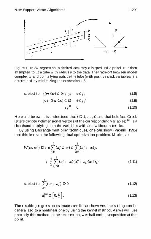
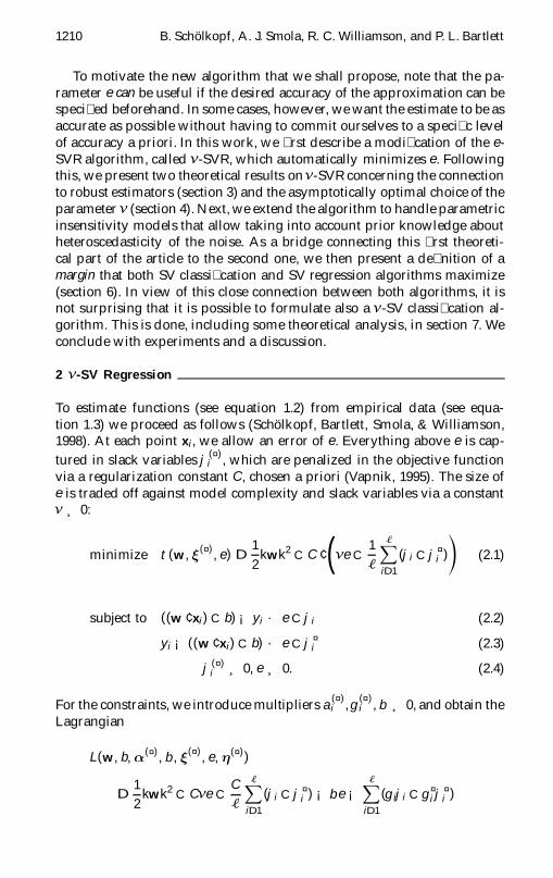
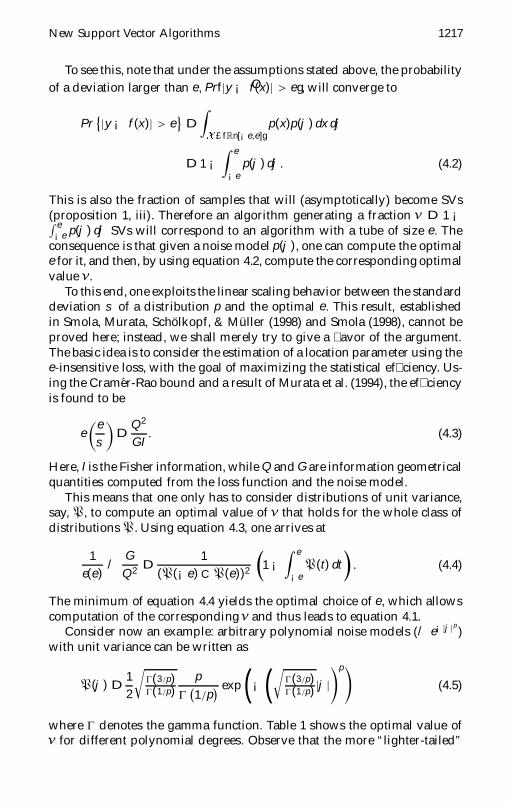
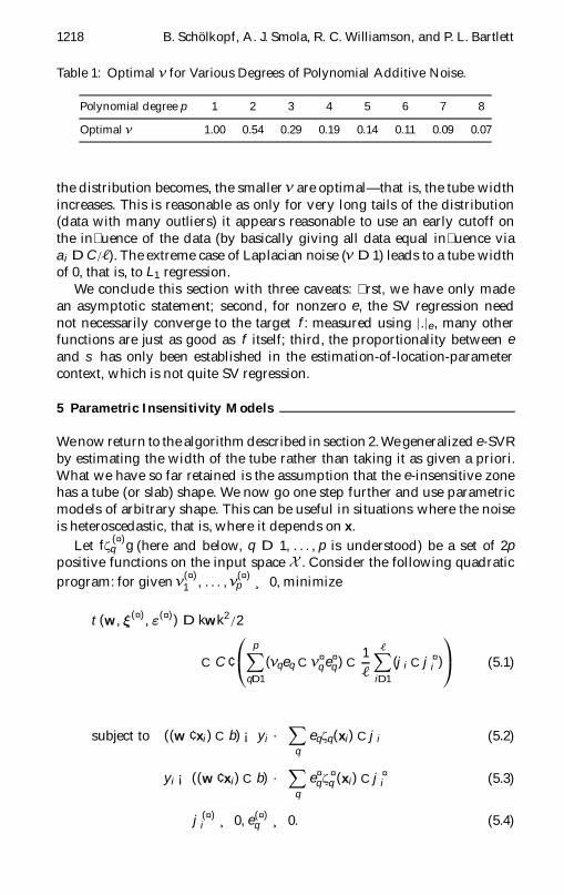
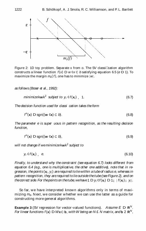
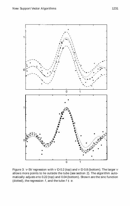
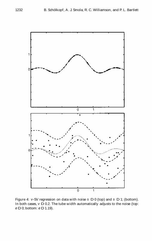
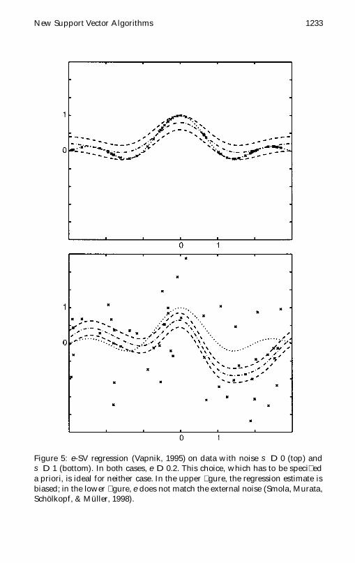
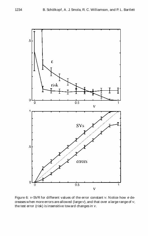
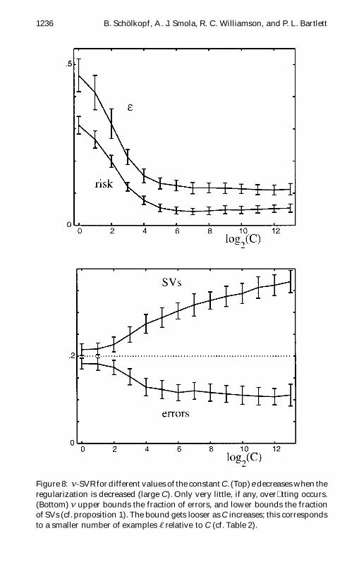
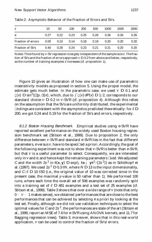
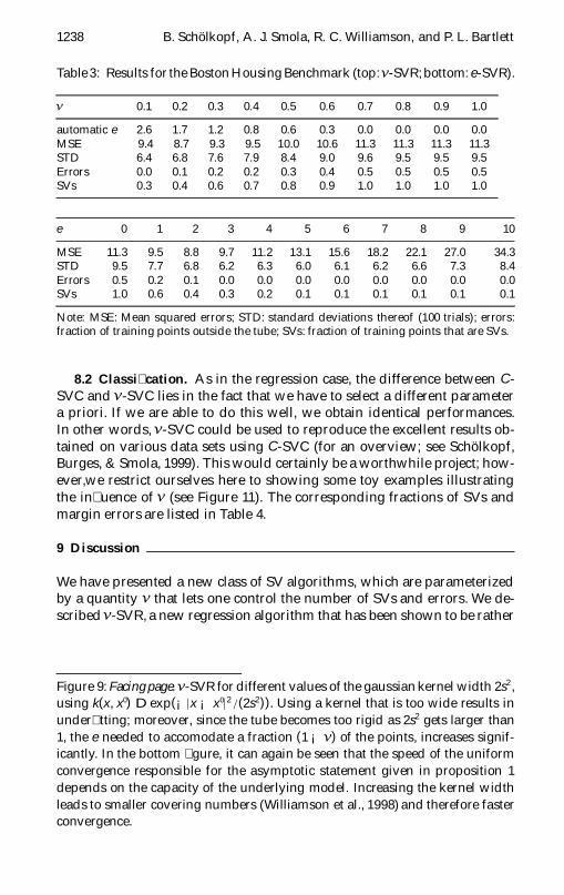
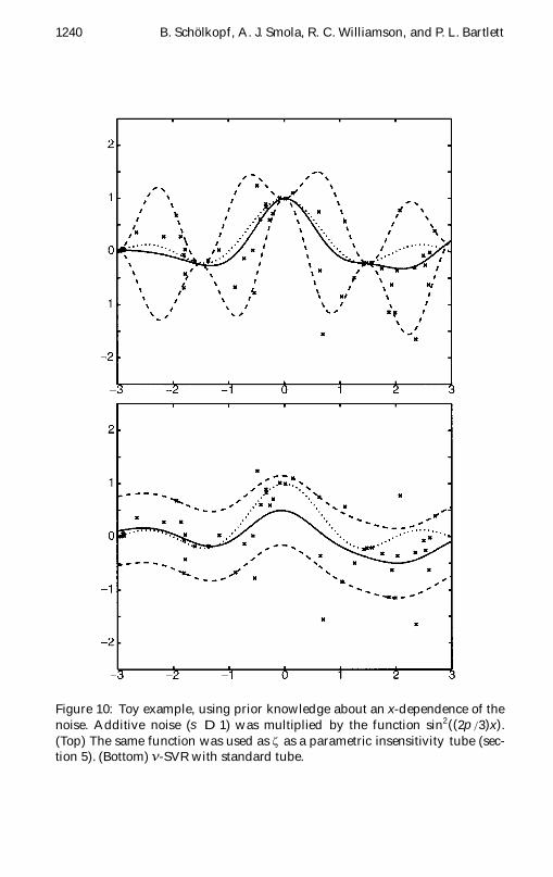
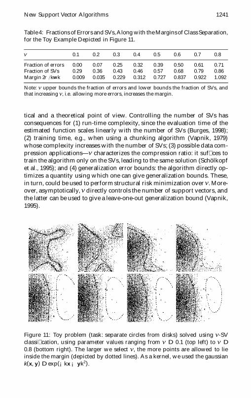based on independent and identically distributed (iid) data

(x1 y1) (x` y ) 2 RN pound R (13)

Here RN is the space in which the input patterns live but most of the fol-lowing also applies for inputs from a set X The goal of the learning processis to nd a function f with a small risk (or test error)

R[ f ] DZ

l( f x y) dP(x y) (14)

where P is the probability measure which is assumed to be responsible forthe generation of the observations (see equation 13) and l is a loss func-tion for example l( f x y) D ( f (x) iexcl y)2 or many other choices (Smola ampScholkopf 1998) The particular loss function for which we would like tominimize equation 14 depends on the specic regression estimation prob-lem at hand This does not necessarily have to coincide with the loss functionused in our learning algorithm First there might be additional constraintsthat we would like our regression estimation to satisfy for instance that ithave a sparse representation in terms of the training data In the SVcase thisis achieved through the insensitive zone in equation 11 Second we cannotminimize equation 14 directly in the rst place since we do not know PInstead we are given the sample equation 13 and we try to obtain a smallrisk by minimizing the regularized risk functional

12

kwk2 C C cent Reemp[ f ] (15)

Here kwk2 is a term that characterizes the model complexity

Reemp[ f ] D

1`

X

iD1

|yi iexcl f (xi)|e (16)

measures the e-insensitive training error and C is a constant determiningthe trade-off In short minimizing equation 15 captures the main insightof statistical learning theory stating that in order to obtain a small risk oneneeds to control both training error and model complexitymdashthat is explainthe data with a simple model

The minimization of equation 15 is equivalent to the following con-strained optimization problem (see Figure 1)

minimize t (w raquo(curren)) D 12

kwk2 C C cent 1`

X

iD1

(ji C j curreni ) (17)









iD1

(acurreni C ai) C

X

iD1


iexcl 12

X

i jD1



subject toX

iD1


a(curren)i 2

h0 C

`

i (113)









12


X

iD1

(ji C j curreni )

(21)







D 12

kwk2 C Cordme CC`

X

iD1


X

iD1

(giji C gcurreni j

curreni )


iexclX

iD1


iexclX

iD1

acurreni (j curren






w DX

i(acurren

i iexcl ai)xi (26)

C centordm iexclX

i(ai C acurren

i ) iexcl b D0 (27)

X

iD1


C`


(curren)i D0 (29)




k(x y) D (W(x) cent W(y)) (210)








iD1


iexcl 12

X

i jD1



subject toX

iD1


a(curren)i 2

h0 C

`

i(213)

X

iD1



f (x) DX

iD1



Pj(a









Pi | f (bi) iexcl










(curren)i gt 0


(curren)i could






supft


shyshyxcent

lt d (c ) (216)


Pr (supf


acutegt a

lt c1ciexcl`

2






Pi a








PìD1(acurren






























sP( y

s) s gt 0g Moreover


ordm D 1 iexclZ e

iexcleP(t) dt where

e D argmint


iexcl1 iexcl

Z t

iexclt

P(t) dtcent

(41)






ordfD

Z


D 1 iexclZ e

iexclep(j ) dj (42)




esup3e

s

acuteD

Q2

GI (43)



1e(e)

GQ2 D


iexcl1 iexcl

Z e

iexcleP(t) dt

cent (44)



P(j ) D 12

rC(3 p)C(1 p)

pC

iexcl1 p

cent exp(iexcl(r

C(3 p)C(1 p) |j |

p(45)





Optimal ordm 100 054 029 019 014 011 009 007









p cedil 0 minimize


C C cent

0

pX

qD1


q ) C1`

X

iD1

(ji C j curreni )

1

A (51)


qeqfq(xi) C ji (52)


qecurren


i (53)


q cedil 0 (54)



X

iD1

a(curren)i f


q (55)




X

iD1







PìD1 a




i ordm`Pif (xi)


ii ordm`Pif (xi)






















cent(62)


cent (63)




L


L cedil 2eL






minf| f (x)| x 2 X g D1 (65)


















me( f ) cedil 2e

kWk (611)








t(w raquo) D12

kwk2 C C`

X

iji (71)

subject to







t (w raquor ) D12

kwk2 iexclordmr C1`

X

iji (73)







kwk2 iexclordmr C1`

X

iji

iexclX


iexcldr (76)


w DX

iaiyixi (77)

ai C bi D1 0 DX

iaiyi

X




W(reg) Diexcl12

X

ij



subject to


0 DX

iaiyi (711)

X



f curren(x) Dsgn(X

iaiyik(x xi) C b

(713)




Pi ji) (ie



b Diexcl 12s

X

x2SC [Siexcl

X

j

ajyjk(x xj) (714)

r D 12s

0

X

x2SC

X

j

ajyjk(x xj) iexclX

x2Siexcl

X

j

ajyjk(x xj)

1

A (715)


Rremp[ f ] D

1`

























w DX

ic izi (717)








X

iaiyizi D

X

i6Dma0

iyizi C amymz0m
















q2`

iexclln N (F l2`


(718)







at scale r satises


shyshyshyc2R2

r 21n log2

iexcl1 C `

n

centcedil 1

oiexcl 1 (720)




r 2 log2 ìexcl 1 (721)




with f (x) DP



s2`

iexcl4c2kwk2


middot ordm C

s2`

iexcl4c2kwk2








8 Experiments



6


through 9


















` 10 50 100 200 500 1000 1500 2000

e 027 022 023 025 026 026 026 026


Fraction of SVs 040 028 024 023 021 021 020 020








ordm 01 02 03 04 05 06 07 08 09 10


e 0 1 2 3 4 5 6 7 8 9 10




9 Discussion









ordm 01 02 03 04 05 06 07 08









Acknowledgments


References




















































iD1

(acurreni C ai) C

X

iD1


iexcl 12

X

i jD1



subject toX

iD1


a(curren)i 2

h0 C

`

i (113)









12


X

iD1

(ji C j curreni )

(21)







D 12

kwk2 C Cordme CC`

X

iD1


X

iD1

(giji C gcurreni j

curreni )


iexclX

iD1


iexclX

iD1

acurreni (j curren






w DX

i(acurren

i iexcl ai)xi (26)

C centordm iexclX

i(ai C acurren

i ) iexcl b D0 (27)

X

iD1


C`


(curren)i D0 (29)




k(x y) D (W(x) cent W(y)) (210)








iD1


iexcl 12

X

i jD1



subject toX

iD1


a(curren)i 2

h0 C

`

i(213)

X

iD1



f (x) DX

iD1



Pj(a









Pi | f (bi) iexcl










(curren)i gt 0


(curren)i could






supft


shyshyxcent

lt d (c ) (216)


Pr (supf


acutegt a

lt c1ciexcl`

2






Pi a








PìD1(acurren






























sP( y

s) s gt 0g Moreover


ordm D 1 iexclZ e

iexcleP(t) dt where

e D argmint


iexcl1 iexcl

Z t

iexclt

P(t) dtcent

(41)






ordfD

Z


D 1 iexclZ e

iexclep(j ) dj (42)




esup3e

s

acuteD

Q2

GI (43)



1e(e)

GQ2 D


iexcl1 iexcl

Z e

iexcleP(t) dt

cent (44)



P(j ) D 12

rC(3 p)C(1 p)

pC

iexcl1 p

cent exp(iexcl(r

C(3 p)C(1 p) |j |

p(45)





Optimal ordm 100 054 029 019 014 011 009 007









p cedil 0 minimize


C C cent

0

pX

qD1


q ) C1`

X

iD1

(ji C j curreni )

1

A (51)


qeqfq(xi) C ji (52)


qecurren


i (53)


q cedil 0 (54)



X

iD1

a(curren)i f


q (55)




X

iD1







PìD1 a




i ordm`Pif (xi)


ii ordm`Pif (xi)






















cent(62)


cent (63)




L


L cedil 2eL






minf| f (x)| x 2 X g D1 (65)


















me( f ) cedil 2e

kWk (611)








t(w raquo) D12

kwk2 C C`

X

iji (71)

subject to







t (w raquor ) D12

kwk2 iexclordmr C1`

X

iji (73)







kwk2 iexclordmr C1`

X

iji

iexclX


iexcldr (76)


w DX

iaiyixi (77)

ai C bi D1 0 DX

iaiyi

X




W(reg) Diexcl12

X

ij



subject to


0 DX

iaiyi (711)

X



f curren(x) Dsgn(X

iaiyik(x xi) C b

(713)




Pi ji) (ie



b Diexcl 12s

X

x2SC [Siexcl

X

j

ajyjk(x xj) (714)

r D 12s

0

X

x2SC

X

j

ajyjk(x xj) iexclX

x2Siexcl

X

j

ajyjk(x xj)

1

A (715)


Rremp[ f ] D

1`

























w DX

ic izi (717)








X

iaiyizi D

X

i6Dma0

iyizi C amymz0m
















q2`

iexclln N (F l2`


(718)







at scale r satises


shyshyshyc2R2

r 21n log2

iexcl1 C `

n

centcedil 1

oiexcl 1 (720)




r 2 log2 ìexcl 1 (721)




with f (x) DP



s2`

iexcl4c2kwk2


middot ordm C

s2`

iexcl4c2kwk2








8 Experiments



6


through 9


















` 10 50 100 200 500 1000 1500 2000

e 027 022 023 025 026 026 026 026


Fraction of SVs 040 028 024 023 021 021 020 020








ordm 01 02 03 04 05 06 07 08 09 10


e 0 1 2 3 4 5 6 7 8 9 10




9 Discussion









ordm 01 02 03 04 05 06 07 08









Acknowledgments


References



















































12


X

iD1

(ji C j curreni )

(21)







D 12

kwk2 C Cordme CC`

X

iD1


X

iD1

(giji C gcurreni j

curreni )


iexclX

iD1


iexclX

iD1

acurreni (j curren






w DX

i(acurren

i iexcl ai)xi (26)

C centordm iexclX

i(ai C acurren

i ) iexcl b D0 (27)

X

iD1


C`


(curren)i D0 (29)




k(x y) D (W(x) cent W(y)) (210)








iD1


iexcl 12

X

i jD1



subject toX

iD1


a(curren)i 2

h0 C

`

i(213)

X

iD1



f (x) DX

iD1



Pj(a









Pi | f (bi) iexcl










(curren)i gt 0


(curren)i could






supft


shyshyxcent

lt d (c ) (216)


Pr (supf


acutegt a

lt c1ciexcl`

2






Pi a








PìD1(acurren






























sP( y

s) s gt 0g Moreover


ordm D 1 iexclZ e

iexcleP(t) dt where

e D argmint


iexcl1 iexcl

Z t

iexclt

P(t) dtcent

(41)






ordfD

Z


D 1 iexclZ e

iexclep(j ) dj (42)




esup3e

s

acuteD

Q2

GI (43)



1e(e)

GQ2 D


iexcl1 iexcl

Z e

iexcleP(t) dt

cent (44)



P(j ) D 12

rC(3 p)C(1 p)

pC

iexcl1 p

cent exp(iexcl(r

C(3 p)C(1 p) |j |

p(45)





Optimal ordm 100 054 029 019 014 011 009 007









p cedil 0 minimize


C C cent

0

pX

qD1


q ) C1`

X

iD1

(ji C j curreni )

1

A (51)


qeqfq(xi) C ji (52)


qecurren


i (53)


q cedil 0 (54)



X

iD1

a(curren)i f


q (55)




X

iD1







PìD1 a




i ordm`Pif (xi)


ii ordm`Pif (xi)






















cent(62)


cent (63)




L


L cedil 2eL






minf| f (x)| x 2 X g D1 (65)


















me( f ) cedil 2e

kWk (611)








t(w raquo) D12

kwk2 C C`

X

iji (71)

subject to







t (w raquor ) D12

kwk2 iexclordmr C1`

X

iji (73)







kwk2 iexclordmr C1`

X

iji

iexclX


iexcldr (76)


w DX

iaiyixi (77)

ai C bi D1 0 DX

iaiyi

X




W(reg) Diexcl12

X

ij



subject to


0 DX

iaiyi (711)

X



f curren(x) Dsgn(X

iaiyik(x xi) C b

(713)




Pi ji) (ie



b Diexcl 12s

X

x2SC [Siexcl

X

j

ajyjk(x xj) (714)

r D 12s

0

X

x2SC

X

j

ajyjk(x xj) iexclX

x2Siexcl

X

j

ajyjk(x xj)

1

A (715)


Rremp[ f ] D

1`

























w DX

ic izi (717)








X

iaiyizi D

X

i6Dma0

iyizi C amymz0m
















q2`

iexclln N (F l2`


(718)







at scale r satises


shyshyshyc2R2

r 21n log2

iexcl1 C `

n

centcedil 1

oiexcl 1 (720)




r 2 log2 ìexcl 1 (721)




with f (x) DP



s2`

iexcl4c2kwk2


middot ordm C

s2`

iexcl4c2kwk2








8 Experiments



6


through 9


















` 10 50 100 200 500 1000 1500 2000

e 027 022 023 025 026 026 026 026


Fraction of SVs 040 028 024 023 021 021 020 020








ordm 01 02 03 04 05 06 07 08 09 10


e 0 1 2 3 4 5 6 7 8 9 10




9 Discussion









ordm 01 02 03 04 05 06 07 08









Acknowledgments


References













































iexclX

iD1


iexclX

iD1

acurreni (j curren






w DX

i(acurren

i iexcl ai)xi (26)

C centordm iexclX

i(ai C acurren

i ) iexcl b D0 (27)

X

iD1


C`


(curren)i D0 (29)




k(x y) D (W(x) cent W(y)) (210)








iD1


iexcl 12

X

i jD1



subject toX

iD1


a(curren)i 2

h0 C

`

i(213)

X

iD1



f (x) DX

iD1



Pj(a









Pi | f (bi) iexcl










(curren)i gt 0


(curren)i could






supft


shyshyxcent

lt d (c ) (216)


Pr (supf


acutegt a

lt c1ciexcl`

2






Pi a








PìD1(acurren






























sP( y

s) s gt 0g Moreover


ordm D 1 iexclZ e

iexcleP(t) dt where

e D argmint


iexcl1 iexcl

Z t

iexclt

P(t) dtcent

(41)






ordfD

Z


D 1 iexclZ e

iexclep(j ) dj (42)




esup3e

s

acuteD

Q2

GI (43)



1e(e)

GQ2 D


iexcl1 iexcl

Z e

iexcleP(t) dt

cent (44)



P(j ) D 12

rC(3 p)C(1 p)

pC

iexcl1 p

cent exp(iexcl(r

C(3 p)C(1 p) |j |

p(45)





Optimal ordm 100 054 029 019 014 011 009 007









p cedil 0 minimize


C C cent

0

pX

qD1


q ) C1`

X

iD1

(ji C j curreni )

1

A (51)


qeqfq(xi) C ji (52)


qecurren


i (53)


q cedil 0 (54)



X

iD1

a(curren)i f


q (55)




X

iD1







PìD1 a




i ordm`Pif (xi)


ii ordm`Pif (xi)






















cent(62)


cent (63)




L


L cedil 2eL






minf| f (x)| x 2 X g D1 (65)


















me( f ) cedil 2e

kWk (611)








t(w raquo) D12

kwk2 C C`

X

iji (71)

subject to







t (w raquor ) D12

kwk2 iexclordmr C1`

X

iji (73)







kwk2 iexclordmr C1`

X

iji

iexclX


iexcldr (76)


w DX

iaiyixi (77)

ai C bi D1 0 DX

iaiyi

X




W(reg) Diexcl12

X

ij



subject to


0 DX

iaiyi (711)

X



f curren(x) Dsgn(X

iaiyik(x xi) C b

(713)




Pi ji) (ie



b Diexcl 12s

X

x2SC [Siexcl

X

j

ajyjk(x xj) (714)

r D 12s

0

X

x2SC

X

j

ajyjk(x xj) iexclX

x2Siexcl

X

j

ajyjk(x xj)

1

A (715)


Rremp[ f ] D

1`

























w DX

ic izi (717)








X

iaiyizi D

X

i6Dma0

iyizi C amymz0m
















q2`

iexclln N (F l2`


(718)







at scale r satises


shyshyshyc2R2

r 21n log2

iexcl1 C `

n

centcedil 1

oiexcl 1 (720)




r 2 log2 ìexcl 1 (721)




with f (x) DP



s2`

iexcl4c2kwk2


middot ordm C

s2`

iexcl4c2kwk2








8 Experiments



6


through 9


















` 10 50 100 200 500 1000 1500 2000

e 027 022 023 025 026 026 026 026


Fraction of SVs 040 028 024 023 021 021 020 020








ordm 01 02 03 04 05 06 07 08 09 10


e 0 1 2 3 4 5 6 7 8 9 10




9 Discussion









ordm 01 02 03 04 05 06 07 08









Acknowledgments


References

















































iD1


iexcl 12

X

i jD1



subject toX

iD1


a(curren)i 2

h0 C

`

i(213)

X

iD1



f (x) DX

iD1



Pj(a









Pi | f (bi) iexcl










(curren)i gt 0


(curren)i could






supft


shyshyxcent

lt d (c ) (216)


Pr (supf


acutegt a

lt c1ciexcl`

2






Pi a








PìD1(acurren






























sP( y

s) s gt 0g Moreover


ordm D 1 iexclZ e

iexcleP(t) dt where

e D argmint


iexcl1 iexcl

Z t

iexclt

P(t) dtcent

(41)






ordfD

Z


D 1 iexclZ e

iexclep(j ) dj (42)




esup3e

s

acuteD

Q2

GI (43)



1e(e)

GQ2 D


iexcl1 iexcl

Z e

iexcleP(t) dt

cent (44)



P(j ) D 12

rC(3 p)C(1 p)

pC

iexcl1 p

cent exp(iexcl(r

C(3 p)C(1 p) |j |

p(45)





Optimal ordm 100 054 029 019 014 011 009 007









p cedil 0 minimize


C C cent

0

pX

qD1


q ) C1`

X

iD1

(ji C j curreni )

1

A (51)


qeqfq(xi) C ji (52)


qecurren


i (53)


q cedil 0 (54)



X

iD1

a(curren)i f


q (55)




X

iD1







PìD1 a




i ordm`Pif (xi)


ii ordm`Pif (xi)






















cent(62)


cent (63)




L


L cedil 2eL






minf| f (x)| x 2 X g D1 (65)


















me( f ) cedil 2e

kWk (611)








t(w raquo) D12

kwk2 C C`

X

iji (71)

subject to







t (w raquor ) D12

kwk2 iexclordmr C1`

X

iji (73)







kwk2 iexclordmr C1`

X

iji

iexclX


iexcldr (76)


w DX

iaiyixi (77)

ai C bi D1 0 DX

iaiyi

X




W(reg) Diexcl12

X

ij



subject to


0 DX

iaiyi (711)

X



f curren(x) Dsgn(X

iaiyik(x xi) C b

(713)




Pi ji) (ie



b Diexcl 12s

X

x2SC [Siexcl

X

j

ajyjk(x xj) (714)

r D 12s

0

X

x2SC

X

j

ajyjk(x xj) iexclX

x2Siexcl

X

j

ajyjk(x xj)

1

A (715)


Rremp[ f ] D

1`

























w DX

ic izi (717)








X

iaiyizi D

X

i6Dma0

iyizi C amymz0m
















q2`

iexclln N (F l2`


(718)







at scale r satises


shyshyshyc2R2

r 21n log2

iexcl1 C `

n

centcedil 1

oiexcl 1 (720)




r 2 log2 ìexcl 1 (721)




with f (x) DP



s2`

iexcl4c2kwk2


middot ordm C

s2`

iexcl4c2kwk2








8 Experiments



6


through 9


















` 10 50 100 200 500 1000 1500 2000

e 027 022 023 025 026 026 026 026


Fraction of SVs 040 028 024 023 021 021 020 020








ordm 01 02 03 04 05 06 07 08 09 10


e 0 1 2 3 4 5 6 7 8 9 10




9 Discussion









ordm 01 02 03 04 05 06 07 08









Acknowledgments


References














































Pi | f (bi) iexcl










(curren)i gt 0


(curren)i could






supft


shyshyxcent

lt d (c ) (216)


Pr (supf


acutegt a

lt c1ciexcl`

2






Pi a








PìD1(acurren






























sP( y

s) s gt 0g Moreover


ordm D 1 iexclZ e

iexcleP(t) dt where

e D argmint


iexcl1 iexcl

Z t

iexclt

P(t) dtcent

(41)






ordfD

Z


D 1 iexclZ e

iexclep(j ) dj (42)




esup3e

s

acuteD

Q2

GI (43)



1e(e)

GQ2 D


iexcl1 iexcl

Z e

iexcleP(t) dt

cent (44)



P(j ) D 12

rC(3 p)C(1 p)

pC

iexcl1 p

cent exp(iexcl(r

C(3 p)C(1 p) |j |

p(45)





Optimal ordm 100 054 029 019 014 011 009 007









p cedil 0 minimize


C C cent

0

pX

qD1


q ) C1`

X

iD1

(ji C j curreni )

1

A (51)


qeqfq(xi) C ji (52)


qecurren


i (53)


q cedil 0 (54)



X

iD1

a(curren)i f


q (55)




X

iD1







PìD1 a




i ordm`Pif (xi)


ii ordm`Pif (xi)






















cent(62)


cent (63)




L


L cedil 2eL






minf| f (x)| x 2 X g D1 (65)


















me( f ) cedil 2e

kWk (611)








t(w raquo) D12

kwk2 C C`

X

iji (71)

subject to







t (w raquor ) D12

kwk2 iexclordmr C1`

X

iji (73)







kwk2 iexclordmr C1`

X

iji

iexclX


iexcldr (76)


w DX

iaiyixi (77)

ai C bi D1 0 DX

iaiyi

X




W(reg) Diexcl12

X

ij



subject to


0 DX

iaiyi (711)

X



f curren(x) Dsgn(X

iaiyik(x xi) C b

(713)




Pi ji) (ie



b Diexcl 12s

X

x2SC [Siexcl

X

j

ajyjk(x xj) (714)

r D 12s

0

X

x2SC

X

j

ajyjk(x xj) iexclX

x2Siexcl

X

j

ajyjk(x xj)

1

A (715)


Rremp[ f ] D

1`

























w DX

ic izi (717)








X

iaiyizi D

X

i6Dma0

iyizi C amymz0m
















q2`

iexclln N (F l2`


(718)







at scale r satises


shyshyshyc2R2

r 21n log2

iexcl1 C `

n

centcedil 1

oiexcl 1 (720)




r 2 log2 ìexcl 1 (721)




with f (x) DP



s2`

iexcl4c2kwk2


middot ordm C

s2`

iexcl4c2kwk2








8 Experiments



6


through 9


















` 10 50 100 200 500 1000 1500 2000

e 027 022 023 025 026 026 026 026


Fraction of SVs 040 028 024 023 021 021 020 020








ordm 01 02 03 04 05 06 07 08 09 10


e 0 1 2 3 4 5 6 7 8 9 10




9 Discussion









ordm 01 02 03 04 05 06 07 08









Acknowledgments


References
















































Pi a








PìD1(acurren






























sP( y

s) s gt 0g Moreover


ordm D 1 iexclZ e

iexcleP(t) dt where

e D argmint


iexcl1 iexcl

Z t

iexclt

P(t) dtcent

(41)






ordfD

Z


D 1 iexclZ e

iexclep(j ) dj (42)




esup3e

s

acuteD

Q2

GI (43)



1e(e)

GQ2 D


iexcl1 iexcl

Z e

iexcleP(t) dt

cent (44)



P(j ) D 12

rC(3 p)C(1 p)

pC

iexcl1 p

cent exp(iexcl(r

C(3 p)C(1 p) |j |

p(45)





Optimal ordm 100 054 029 019 014 011 009 007









p cedil 0 minimize


C C cent

0

pX

qD1


q ) C1`

X

iD1

(ji C j curreni )

1

A (51)


qeqfq(xi) C ji (52)


qecurren


i (53)


q cedil 0 (54)



X

iD1

a(curren)i f


q (55)




X

iD1







PìD1 a




i ordm`Pif (xi)


ii ordm`Pif (xi)






















cent(62)


cent (63)




L


L cedil 2eL






minf| f (x)| x 2 X g D1 (65)


















me( f ) cedil 2e

kWk (611)








t(w raquo) D12

kwk2 C C`

X

iji (71)

subject to







t (w raquor ) D12

kwk2 iexclordmr C1`

X

iji (73)







kwk2 iexclordmr C1`

X

iji

iexclX


iexcldr (76)


w DX

iaiyixi (77)

ai C bi D1 0 DX

iaiyi

X




W(reg) Diexcl12

X

ij



subject to


0 DX

iaiyi (711)

X



f curren(x) Dsgn(X

iaiyik(x xi) C b

(713)




Pi ji) (ie



b Diexcl 12s

X

x2SC [Siexcl

X

j

ajyjk(x xj) (714)

r D 12s

0

X

x2SC

X

j

ajyjk(x xj) iexclX

x2Siexcl

X

j

ajyjk(x xj)

1

A (715)


Rremp[ f ] D

1`

























w DX

ic izi (717)








X

iaiyizi D

X

i6Dma0

iyizi C amymz0m
















q2`

iexclln N (F l2`


(718)







at scale r satises


shyshyshyc2R2

r 21n log2

iexcl1 C `

n

centcedil 1

oiexcl 1 (720)




r 2 log2 ìexcl 1 (721)




with f (x) DP



s2`

iexcl4c2kwk2


middot ordm C

s2`

iexcl4c2kwk2








8 Experiments



6


through 9


















` 10 50 100 200 500 1000 1500 2000

e 027 022 023 025 026 026 026 026


Fraction of SVs 040 028 024 023 021 021 020 020








ordm 01 02 03 04 05 06 07 08 09 10


e 0 1 2 3 4 5 6 7 8 9 10




9 Discussion









ordm 01 02 03 04 05 06 07 08









Acknowledgments


References




































































sP( y

s) s gt 0g Moreover


ordm D 1 iexclZ e

iexcleP(t) dt where

e D argmint


iexcl1 iexcl

Z t

iexclt

P(t) dtcent

(41)






ordfD

Z


D 1 iexclZ e

iexclep(j ) dj (42)




esup3e

s

acuteD

Q2

GI (43)



1e(e)

GQ2 D


iexcl1 iexcl

Z e

iexcleP(t) dt

cent (44)



P(j ) D 12

rC(3 p)C(1 p)

pC

iexcl1 p

cent exp(iexcl(r

C(3 p)C(1 p) |j |

p(45)





Optimal ordm 100 054 029 019 014 011 009 007









p cedil 0 minimize


C C cent

0

pX

qD1


q ) C1`

X

iD1

(ji C j curreni )

1

A (51)


qeqfq(xi) C ji (52)


qecurren


i (53)


q cedil 0 (54)



X

iD1

a(curren)i f


q (55)




X

iD1







P`iD1 a




i ordm`Pif (xi)


ii ordm`Pif (xi)






















cent(62)


cent (63)




L


L cedil 2eL






minf| f (x)| x 2 X g D1 (65)


















me( f ) cedil 2e

kWk (611)








t(w raquo) D12

kwk2 C C`

X

iji (71)

subject to







t (w raquor ) D12

kwk2 iexclordmr C1`

X

iji (73)







kwk2 iexclordmr C1`

X

iji

iexclX


iexcldr (76)


w DX

iaiyixi (77)

ai C bi D1 0 DX

iaiyi

X




W(reg) Diexcl12

X

ij



subject to


0 DX

iaiyi (711)

X



f curren(x) Dsgn(X

iaiyik(x xi) C b

(713)




Pi ji) (ie



b Diexcl 12s

X

x2SC [Siexcl

X

j

ajyjk(x xj) (714)

r D 12s

0

X

x2SC

X

j

ajyjk(x xj) iexclX

x2Siexcl

X

j

ajyjk(x xj)

1

A (715)


Rremp[ f ] D

1`

























w DX

ic izi (717)








X

iaiyizi D

X

i6Dma0

iyizi C amymz0m
















q2`

iexclln N (F l2`


(718)







at scale r satises


shyshyshyc2R2

r 21n log2

iexcl1 C `

n

centcedil 1

oiexcl 1 (720)




r 2 log2 `iexcl 1 (721)




with f (x) DP



s2`

iexcl4c2kwk2


middot ordm C

s2`

iexcl4c2kwk2








8 Experiments



6


through 9


















` 10 50 100 200 500 1000 1500 2000

e 027 022 023 025 026 026 026 026


Fraction of SVs 040 028 024 023 021 021 020 020








ordm 01 02 03 04 05 06 07 08 09 10


e 0 1 2 3 4 5 6 7 8 9 10




9 Discussion









ordm 01 02 03 04 05 06 07 08









Acknowledgments


References















































ordfD

Z


D 1 iexclZ e

iexclep(j ) dj (42)




esup3e

s

acuteD

Q2

GI (43)



1e(e)

GQ2 D


iexcl1 iexcl

Z e

iexcleP(t) dt

cent (44)



P(j ) D 12

rC(3 p)C(1 p)

pC

iexcl1 p

cent exp(iexcl(r

C(3 p)C(1 p) |j |

p(45)





Optimal ordm 100 054 029 019 014 011 009 007









p cedil 0 minimize


C C cent

0

pX

qD1


q ) C1`

X

iD1

(ji C j curreni )

1

A (51)


qeqfq(xi) C ji (52)


qecurren


i (53)


q cedil 0 (54)



X

iD1

a(curren)i f


q (55)




X

iD1







P`iD1 a




i ordm`Pif (xi)


ii ordm`Pif (xi)






















cent(62)


cent (63)




L


L cedil 2eL






minf| f (x)| x 2 X g D1 (65)


















me( f ) cedil 2e

kWk (611)








t(w raquo) D12

kwk2 C C`

X

iji (71)

subject to







t (w raquor ) D12

kwk2 iexclordmr C1`

X

iji (73)







kwk2 iexclordmr C1`

X

iji

iexclX


iexcldr (76)


w DX

iaiyixi (77)

ai C bi D1 0 DX

iaiyi

X




W(reg) Diexcl12

X

ij



subject to


0 DX

iaiyi (711)

X



f curren(x) Dsgn(X

iaiyik(x xi) C b

(713)




Pi ji) (ie



b Diexcl 12s

X

x2SC [Siexcl

X

j

ajyjk(x xj) (714)

r D 12s

0

X

x2SC

X

j

ajyjk(x xj) iexclX

x2Siexcl

X

j

ajyjk(x xj)

1

A (715)


Rremp[ f ] D

1`

























w DX

ic izi (717)








X

iaiyizi D

X

i6Dma0

iyizi C amymz0m
















q2`

iexclln N (F l2`


(718)







at scale r satises


shyshyshyc2R2

r 21n log2

iexcl1 C `

n

centcedil 1

oiexcl 1 (720)




r 2 log2 `iexcl 1 (721)




with f (x) DP



s2`

iexcl4c2kwk2


middot ordm C

s2`

iexcl4c2kwk2








8 Experiments



6


through 9


















` 10 50 100 200 500 1000 1500 2000

e 027 022 023 025 026 026 026 026


Fraction of SVs 040 028 024 023 021 021 020 020








ordm 01 02 03 04 05 06 07 08 09 10


e 0 1 2 3 4 5 6 7 8 9 10




9 Discussion









ordm 01 02 03 04 05 06 07 08









Acknowledgments


References















































Optimal ordm 100 054 029 019 014 011 009 007









p cedil 0 minimize


C C cent

0

pX

qD1


q ) C1`

X

iD1

(ji C j curreni )

1

A (51)


qeqfq(xi) C ji (52)


qecurren


i (53)


q cedil 0 (54)



X

iD1

a(curren)i f


q (55)




X

iD1







P`iD1 a




i ordm`Pif (xi)


ii ordm`Pif (xi)






















cent(62)


cent (63)




L


L cedil 2eL






minf| f (x)| x 2 X g D1 (65)


















me( f ) cedil 2e

kWk (611)








t(w raquo) D12

kwk2 C C`

X

iji (71)

subject to







t (w raquor ) D12

kwk2 iexclordmr C1`

X

iji (73)







kwk2 iexclordmr C1`

X

iji

iexclX


iexcldr (76)


w DX

iaiyixi (77)

ai C bi D1 0 DX

iaiyi

X




W(reg) Diexcl12

X

ij



subject to


0 DX

iaiyi (711)

X



f curren(x) Dsgn(X

iaiyik(x xi) C b

(713)




Pi ji) (ie



b Diexcl 12s

X

x2SC [Siexcl

X

j

ajyjk(x xj) (714)

r D 12s

0

X

x2SC

X

j

ajyjk(x xj) iexclX

x2Siexcl

X

j

ajyjk(x xj)

1

A (715)


Rremp[ f ] D

1`

























w DX

ic izi (717)








X

iaiyizi D

X

i6Dma0

iyizi C amymz0m
















q2`

iexclln N (F l2`


(718)







at scale r satises


shyshyshyc2R2

r 21n log2

iexcl1 C `

n

centcedil 1

oiexcl 1 (720)




r 2 log2 `iexcl 1 (721)




with f (x) DP



s2`

iexcl4c2kwk2


middot ordm C

s2`

iexcl4c2kwk2








8 Experiments



6


through 9


















` 10 50 100 200 500 1000 1500 2000

e 027 022 023 025 026 026 026 026


Fraction of SVs 040 028 024 023 021 021 020 020








ordm 01 02 03 04 05 06 07 08 09 10


e 0 1 2 3 4 5 6 7 8 9 10




9 Discussion









ordm 01 02 03 04 05 06 07 08









Acknowledgments


References














































X

iD1

a(curren)i f


q (55)




X

iD1







P`iD1 a




i ordm`Pif (xi)


ii ordm`Pif (xi)






















cent(62)


cent (63)




L


L cedil 2eL






minf| f (x)| x 2 X g D1 (65)


















me( f ) cedil 2e

kWk (611)








t(w raquo) D12

kwk2 C C`

X

iji (71)

subject to







t (w raquor ) D12

kwk2 iexclordmr C1`

X

iji (73)







kwk2 iexclordmr C1`

X

iji

iexclX


iexcldr (76)


w DX

iaiyixi (77)

ai C bi D1 0 DX

iaiyi

X




W(reg) Diexcl12

X

ij



subject to


0 DX

iaiyi (711)

X



f curren(x) Dsgn(X

iaiyik(x xi) C b

(713)




Pi ji) (ie



b Diexcl 12s

X

x2SC [Siexcl

X

j

ajyjk(x xj) (714)

r D 12s

0

X

x2SC

X

j

ajyjk(x xj) iexclX

x2Siexcl

X

j

ajyjk(x xj)

1

A (715)


Rremp[ f ] D

1`

























w DX

ic izi (717)








X

iaiyizi D

X

i6Dma0

iyizi C amymz0m
















q2`

iexclln N (F l2`


(718)







at scale r satises


shyshyshyc2R2

r 21n log2

iexcl1 C `

n

centcedil 1

oiexcl 1 (720)




r 2 log2 `iexcl 1 (721)




with f (x) DP



s2`

iexcl4c2kwk2


middot ordm C

s2`

iexcl4c2kwk2








8 Experiments



6


through 9


















` 10 50 100 200 500 1000 1500 2000

e 027 022 023 025 026 026 026 026


Fraction of SVs 040 028 024 023 021 021 020 020








ordm 01 02 03 04 05 06 07 08 09 10


e 0 1 2 3 4 5 6 7 8 9 10




9 Discussion









ordm 01 02 03 04 05 06 07 08









Acknowledgments


References






























































cent(62)


cent (63)




L


L cedil 2eL






minf| f (x)| x 2 X g D1 (65)


















me( f ) cedil 2e

kWk (611)








t(w raquo) D12

kwk2 C C`

X

iji (71)

subject to







t (w raquor ) D12

kwk2 iexclordmr C1`

X

iji (73)







kwk2 iexclordmr C1`

X

iji

iexclX


iexcldr (76)


w DX

iaiyixi (77)

ai C bi D1 0 DX

iaiyi

X




W(reg) Diexcl12

X

ij



subject to


0 DX

iaiyi (711)

X



f curren(x) Dsgn(X

iaiyik(x xi) C b

(713)




Pi ji) (ie



b Diexcl 12s

X

x2SC [Siexcl

X

j

ajyjk(x xj) (714)

r D 12s

0

X

x2SC

X

j

ajyjk(x xj) iexclX

x2Siexcl

X

j

ajyjk(x xj)

1

A (715)


Rremp[ f ] D

1`

























w DX

ic izi (717)








X

iaiyizi D

X

i6Dma0

iyizi C amymz0m
















q2`

iexclln N (F l2`


(718)







at scale r satises


shyshyshyc2R2

r 21n log2

iexcl1 C `

n

centcedil 1

oiexcl 1 (720)




r 2 log2 `iexcl 1 (721)




with f (x) DP



s2`

iexcl4c2kwk2


middot ordm C

s2`

iexcl4c2kwk2








8 Experiments



6


through 9


















` 10 50 100 200 500 1000 1500 2000

e 027 022 023 025 026 026 026 026


Fraction of SVs 040 028 024 023 021 021 020 020








ordm 01 02 03 04 05 06 07 08 09 10


e 0 1 2 3 4 5 6 7 8 9 10




9 Discussion









ordm 01 02 03 04 05 06 07 08









Acknowledgments


References



























































me( f ) cedil 2e

kWk (611)








t(w raquo) D12

kwk2 C C`

X

iji (71)

subject to







t (w raquor ) D12

kwk2 iexclordmr C1`

X

iji (73)







kwk2 iexclordmr C1`

X

iji

iexclX


iexcldr (76)


w DX

iaiyixi (77)

ai C bi D1 0 DX

iaiyi

X




W(reg) Diexcl12

X

ij



subject to


0 DX

iaiyi (711)

X



f curren(x) Dsgn(X

iaiyik(x xi) C b

(713)




Pi ji) (ie



b Diexcl 12s

X

x2SC [Siexcl

X

j

ajyjk(x xj) (714)

r D 12s

0

X

x2SC

X

j

ajyjk(x xj) iexclX

x2Siexcl

X

j

ajyjk(x xj)

1

A (715)


Rremp[ f ] D

1`

























w DX

ic izi (717)








X

iaiyizi D

X

i6Dma0

iyizi C amymz0m
















q2`

iexclln N (F l2`


(718)







at scale r satises


shyshyshyc2R2

r 21n log2

iexcl1 C `

n

centcedil 1

oiexcl 1 (720)




r 2 log2 `iexcl 1 (721)




with f (x) DP



s2`

iexcl4c2kwk2


middot ordm C

s2`

iexcl4c2kwk2








8 Experiments



6


through 9


















` 10 50 100 200 500 1000 1500 2000

e 027 022 023 025 026 026 026 026


Fraction of SVs 040 028 024 023 021 021 020 020








ordm 01 02 03 04 05 06 07 08 09 10


e 0 1 2 3 4 5 6 7 8 9 10




9 Discussion









ordm 01 02 03 04 05 06 07 08









Acknowledgments


References














































t (w raquor ) D12

kwk2 iexclordmr C1`

X

iji (73)







kwk2 iexclordmr C1`

X

iji

iexclX


iexcldr (76)


w DX

iaiyixi (77)

ai C bi D1 0 DX

iaiyi

X




W(reg) Diexcl12

X

ij



subject to


0 DX

iaiyi (711)

X



f curren(x) Dsgn(X

iaiyik(x xi) C b

(713)




Pi ji) (ie



b Diexcl 12s

X

x2SC [Siexcl

X

j

ajyjk(x xj) (714)

r D 12s

0

X

x2SC

X

j

ajyjk(x xj) iexclX

x2Siexcl

X

j

ajyjk(x xj)

1

A (715)


Rremp[ f ] D

1`

























w DX

ic izi (717)








X

iaiyizi D

X

i6Dma0

iyizi C amymz0m
















q2`

iexclln N (F l2`


(718)







at scale r satises


shyshyshyc2R2

r 21n log2

iexcl1 C `

n

centcedil 1

oiexcl 1 (720)




r 2 log2 `iexcl 1 (721)




with f (x) DP



s2`

iexcl4c2kwk2


middot ordm C

s2`

iexcl4c2kwk2








8 Experiments



6


through 9


















` 10 50 100 200 500 1000 1500 2000

e 027 022 023 025 026 026 026 026


Fraction of SVs 040 028 024 023 021 021 020 020








ordm 01 02 03 04 05 06 07 08 09 10


e 0 1 2 3 4 5 6 7 8 9 10




9 Discussion









ordm 01 02 03 04 05 06 07 08









Acknowledgments


References













































subject to


0 DX

iaiyi (711)

X



f curren(x) Dsgn(X

iaiyik(x xi) C b

(713)




Pi ji) (ie



b Diexcl 12s

X

x2SC [Siexcl

X

j

ajyjk(x xj) (714)

r D 12s

0

X

x2SC

X

j

ajyjk(x xj) iexclX

x2Siexcl

X

j

ajyjk(x xj)

1

A (715)


Rremp[ f ] D

1`

























w DX

ic izi (717)








X

iaiyizi D

X

i6Dma0

iyizi C amymz0m
















q2`

iexclln N (F l2`


(718)







at scale r satises


shyshyshyc2R2

r 21n log2

iexcl1 C `

n

centcedil 1

oiexcl 1 (720)




r 2 log2 `iexcl 1 (721)




with f (x) DP



s2`

iexcl4c2kwk2


middot ordm C

s2`

iexcl4c2kwk2








8 Experiments



6


through 9


















` 10 50 100 200 500 1000 1500 2000

e 027 022 023 025 026 026 026 026


Fraction of SVs 040 028 024 023 021 021 020 020








ordm 01 02 03 04 05 06 07 08 09 10


e 0 1 2 3 4 5 6 7 8 9 10




9 Discussion









ordm 01 02 03 04 05 06 07 08









Acknowledgments


References



































































w DX

ic izi (717)








X

iaiyizi D

X

i6Dma0

iyizi C amymz0m
















q2`

iexclln N (F l2`


(718)







at scale r satises


shyshyshyc2R2

r 21n log2

iexcl1 C `

n

centcedil 1

oiexcl 1 (720)




r 2 log2 `iexcl 1 (721)




with f (x) DP



s2`

iexcl4c2kwk2


middot ordm C

s2`

iexcl4c2kwk2








8 Experiments



6


through 9


















` 10 50 100 200 500 1000 1500 2000

e 027 022 023 025 026 026 026 026


Fraction of SVs 040 028 024 023 021 021 020 020








ordm 01 02 03 04 05 06 07 08 09 10


e 0 1 2 3 4 5 6 7 8 9 10




9 Discussion









ordm 01 02 03 04 05 06 07 08









Acknowledgments


References
















































X

iaiyizi D

X

i6Dma0

iyizi C amymz0m
















q2`

iexclln N (F l2`


(718)







at scale r satises


shyshyshyc2R2

r 21n log2

iexcl1 C `

n

centcedil 1

oiexcl 1 (720)




r 2 log2 `iexcl 1 (721)




with f (x) DP



s2`

iexcl4c2kwk2


middot ordm C

s2`

iexcl4c2kwk2








8 Experiments



6


through 9


















` 10 50 100 200 500 1000 1500 2000

e 027 022 023 025 026 026 026 026


Fraction of SVs 040 028 024 023 021 021 020 020








ordm 01 02 03 04 05 06 07 08 09 10


e 0 1 2 3 4 5 6 7 8 9 10




9 Discussion









ordm 01 02 03 04 05 06 07 08









Acknowledgments


References















































q2`

iexclln N (F l2`


(718)







at scale r satises


shyshyshyc2R2

r 21n log2

iexcl1 C `

n

centcedil 1

oiexcl 1 (720)




r 2 log2 `iexcl 1 (721)




with f (x) DP



s2`

iexcl4c2kwk2


middot ordm C

s2`

iexcl4c2kwk2








8 Experiments



6


through 9


















` 10 50 100 200 500 1000 1500 2000

e 027 022 023 025 026 026 026 026


Fraction of SVs 040 028 024 023 021 021 020 020








ordm 01 02 03 04 05 06 07 08 09 10


e 0 1 2 3 4 5 6 7 8 9 10




9 Discussion









ordm 01 02 03 04 05 06 07 08









Acknowledgments


References













































with f (x) DP



s2`

iexcl4c2kwk2


middot ordm C

s2`

iexcl4c2kwk2








8 Experiments



6


through 9


















` 10 50 100 200 500 1000 1500 2000

e 027 022 023 025 026 026 026 026


Fraction of SVs 040 028 024 023 021 021 020 020








ordm 01 02 03 04 05 06 07 08 09 10


e 0 1 2 3 4 5 6 7 8 9 10




9 Discussion









ordm 01 02 03 04 05 06 07 08









Acknowledgments


References




























































` 10 50 100 200 500 1000 1500 2000

e 027 022 023 025 026 026 026 026


Fraction of SVs 040 028 024 023 021 021 020 020








ordm 01 02 03 04 05 06 07 08 09 10


e 0 1 2 3 4 5 6 7 8 9 10




9 Discussion









ordm 01 02 03 04 05 06 07 08









Acknowledgments


References














































ordm 01 02 03 04 05 06 07 08 09 10


e 0 1 2 3 4 5 6 7 8 9 10




9 Discussion









ordm 01 02 03 04 05 06 07 08









Acknowledgments


References


















































ordm 01 02 03 04 05 06 07 08









Acknowledgments


References
















































Acknowledgments


References












































new support vector algorithms - purdue universityyuzhu/stat598m3/papers/newsv… · ·...

Documents