new quantitative models of banking supervision - …df69f8e1-ebcb-4fcf-8a60-5bb8b3f48223/... · the...

≈√

New Quantitative Modelsof Banking Supervision

Cooperation of Austrian Financial Market Authority and Oesterreichische Nationalbank

Vienna, © 2004

New Quant i t a t i ve Mode l s

o f Bank ing Superv i s i on

ˆ

Oe s t erre i ch i s che Nat ionalbank

Published by:Oesterreichische Nationalbank (OeNB)Otto-Wagner-Platz 3, 1090 ViennaAustrian Financial Market Authority (FMA)Praterstrasse 23, 1020 Vienna

Produced by:Oesterreichische Nationalbank

Edited by:Gerhard Coosmann, Doris Datschetzky, Evgenia Glogova, Markus Hameter,Evelyn Hayden, Andreas Ho‹ger, Johannes Turner, (all OeNB)Ju‹rgen Bauer, Wolfgang Errath, Stephan Unterberger (all FMA)

Design:Peter Buchegger, Secretariat of the Governing Board and Public Relations (OeNB)

Typesetting, printing, and production:OeNB Printing Office

Published and produced at:Otto-Wagner-Platz 3, 1090 Vienna, Austria

Inquiries:Oesterreichische NationalbankAustrian Financial Market Authority (FMA)

Secretariat of the Governing Board and Public RelationsOtto-Wagner-Platz 3, 1090 Vienna, AustriaPostal address: PO Box 61, 1011 Vienna, AustriaPhone: (+43-1) 40420-6666Fax: (+43-1) 40420-6696

Orders:Oesterreichische NationalbankDocumentation Management and Communication SystemsOtto-Wagner-Platz 3, 1090 Vienna, AustriaPostal address: PO Box 61, 1011 Vienna, AustriaPhone: (+43-1) 40420-2345Fax: (+43-1) 40420-2398

Internet:http://www.oenb.athttp://www.fma.gv.at

Paper:Salzer Demeter, 100% woodpulp paper, bleached without chlorine, acid-free, without optical whiteners

DVR 0031577

Vienna 2004

A reliable and financially sound banking sector is an essential prerequisite for acountry�s stability and economic growth. For this reason, monitoring and exam-ining the financial situation of banks is of great interest to regulatory authoritiesthroughout the world. Regulators — even within the EU — use a variety ofapproaches to attain this goal, which is due to the different structures not onlyof the authorities themselves but even more so of the financial centers (inparticular the number of banks). As on-site audits require substantial amountsof time and resources and cannot be carried out very frequently due to the largenumber of banks in Austria, off-site analyses play a major role in the supervisionprocess. Therefore, the Oesterreichische Nationalbank (OeNB) and theAustrian Financial Market Authority (FMA) place great emphasis on developingand implementing sophisticated, up-to-date off-site analysis models to make fulluse of the resources of both institutions.

The analysis tools used so far turned out to be successful and will continueto exist in a slightly modified form. However, shifting the focus to risk-basedsupervision has made it necessary to concentrate on the individual risks perse in certain segments and thus to review and expand off-site analysis withregard to risk-based aspects.

As a result, the OeNB and the FMA decided — with university support — toadvance the Austrian analysis landscape in a fundamental manner. Thispublication contains an overview of the new core models; a detailed descriptionof the entire analysis landscape will be made available at the beginning of nextyear.

We are especially grateful to the employees of both institutions who wereinvolved in the project in general and this publication in particular and whodistinguished themselves with their expertise and dedication.

That said, we hope we have aroused your interest with this publication on�New Quantitative Models of Banking Supervision�.

Vienna, July 2004

Michael HysekHead of Banking Supervision Department,

FMA

Andreas IttnerDirector Financial Institutions

and Markets, OeNB

Preface

Models of Banking Supervision 3

STATISTICAL MODEL

1 Theory 91.1 Discriminant Analysis 101.2 Logit and Probit Models 111.3 Cox Model 121.4 Neural Networks 141.5 Computer-aided Classification Methods 14

2 Database 152.1 Data Retrieval and Preparation 152.2 Data Aggregation and Indicator Determination 17

3 Development of the Logit Model 173.1 Transformation of Input Variables 173.2 Determination of Data Set for Model Estimation 183.3 Definition of Estimation and Validation Samples 183.4 Estimation of Univariate Models 193.5 Estimation of Multivariate Models 203.6 Calibration 223.7 Presentation of Results 23

4 Development of the Logit Model 244.1 Descriptive Analyses 244.2 Statistical Tests 24

5 Development of the Cox Model 255.1 Cox Proportional Hazard Rate Model 255.2 Further Development of the Cox Model 27

6 Summary 27

STRUCTURAL MODEL

7 Aggregation of Risks 307.1 Theoretical Background 307.2 Risk Aggregation within Individual Risk Categories 317.3 Aggregation across the Individual Risk Categories 337.4 Selected Procedure 37

8 Credit Risk 388.1 Description of Method Used to Compute Credit Risk 408.2 Database 428.3 Preparation of Input Variables 458.4 Detailed Description of the Model 488.5 Presentation of Results 518.6 Further Development of the Model 51

Table of Contents

4 Models of Banking Supervision

9 Marktrisk 539.1 Description of the Methods Used to Determine Market Risk 539.2 Data Model 559.3 Transformation of Reported Data into Risk Loads 579.4 Detailed Description of the Model 58

10 Operational Risk 5910.1 Significance of the Operational Risk 5910.2 Basel II and the Determination of Operational Risk 6010.3 Selected Procedure 62

11 Capacity to Cover Losses (Reserves) 6411.1 Classification of Risk Coverage Capital 6411.2 Composition of Capacity to Cover Losses 67

12 Assessment of Total Risk 6712.1 Theoretical Background 6812.2 Derivation of Implied Default Probabilities 6812.3 Reviewing Adherence to Equilibrium Conditions 69

13 Summary 70

ANNEX

14 Index of Illustrations 74

15 References 75

Table of Contents


Off-site analysis can use the following methods in the assessment of banks: (i) asimple observation and analysis of balance-sheet indicators, income statement,and other indicators from which the deterioration of a bank�s individual positioncan be derived by experts in an early-warning system (�supervisory screens�);and (ii) a statistical (econometric) analysis of these indicators (or general exog-enous variables) that makes it possible to estimate a bank�s probability of defaultor its rating.

This publication describes approaches of the latter category. Specifically, wehave selected statistical methods of off-site bank analysis which use econometricmethods as well as structural approaches in an attempt to realize, assess, andgenerally quantify problematic bank situations more effectively.

The first part of this publication describes the procedures selected from theclass of statistical models. Using logit regression, it is possible to estimate theprobabilities of occurrence for certain bank problems based on highly aggre-gated indicators gathered from banking statistics reports. Building on thoseresults, a Cox model can be used to compute the distance to default in orderto determine the urgency of potential measures.

The second part of this publication deals with the development of astructural model for all Austrian banks. While statistical models forecast abank�s default potential by observing indicators closely correlated with theevent, the structural approach is meant to offer an economic model whichcan explain causal relations and thus reveal the source of risks in order to enablean evaluation of the reasons underlying such problematic developments. Initialattempts to do so using market-based approaches (stock prices, interest-ratespreads) were rejected due to data restrictions. In the end, the decision tomodel the most important types of risks (credit, market, and operational risks)and to compute individual value at risk proved to be rewarding.

In this document, we will describe the methods, data input, results and alsonecessary assumptions and simplifications used in modeling. The potentialanalyses in the structural model are manifold and range from classic coveragecapacity calculation (comparison of reserves and risks per defined defaultprobability) to the calculation of expected and unexpected losses (includingthe related calculation of economic capital) and the possibility of simulatingchanges by altering input parameters (e.g., industry defaults, interest ratechanges, etc.).

Introduction


Stat i s t i cal Model

Methods and Calculat ion s

IntroductionStatistical models of off-site analysis involve a search for explanatory variablesthat provide as sound and reliable a forecast of the deterioration of a bank�ssituation as possible. In this study, the search for such explanatory variableswas not merely limited to the balance sheets of banks.1 The entire supervisoryreporting system was included, and macroeconomic indicators were alsoexamined as to their ability to explain bank defaults. In a multi-step procedure,a multitude of potential variables were reduced to those which together showedthe highest explanatory value with regard to bank defaults in a multivariatemodel.

In selecting the statistical model, the choice was made to focus on develop-ing a logit model. Logit models are certainly the current standard among off-site analysis models, both in their practical application by regulators and inthe academic literature. The results produced by such models can be inter-preted directly as default probabilities, which sets the results apart from the out-put of CAMEL ratings,2 for example (in the Austrian CAMEL rating system,banks are ranked only in relation to one other, and it is not possible to makestatements concerning the default probability of a single bank).

One potential problem with the logit model (and with regression modelsusing cross-section data in general) is the fact that such approaches do notdirectly take into account the time at which a bank�s default occurs. This disad-vantage can be remedied by means of the Cox model, as the hazard rate is usedto estimate the time to default explicitly as an additional component in theeconometric model. For this reason, a Cox model was developed to accompanythe logit model.

The basic procedure used to develop the logit model is outlined below; adetailed description will be given in the sections that follow.

The first step involved collecting, preparing, and examining the data. Forthis purpose, the entire supervision reporting system, the Major Loans Register,and external data such as time series of macroeconomic indicators wereaccessed. These data were combined in a database which is managed by suitablestatistical software.

Next, the data were aggregated and the indicators were defined. The MajorLoans Register was also included in connection with data from the Kredit-schutzverband von 1870 (KSV), and other sources. Overall, 291 ratios werecomputed and then subjected to univariate tests.

This was followed by extensive quality control measures. It was necessary toexamine the individual indicators to check, for example, whether the valueswere within certain logical ranges, etc. Some indicators were transformed if thisproved necessary for procedural reasons.

Next, estimation and validation samples were generated for the subsequentunivariate and multivariate modeling in order to enable verification of the logitmodel�s predictive power.

1 For simplicity�s sake, the terms �defaults� and �default probabilities� will be used in this document to refer to events in whichbanks suffer problems which make it doubtful whether they could survive without intervention (e.g. industry subsidies).

2 CAMEL is short for Capital, Assets, Management, Earnings, and Liquidity. For a detailed description, please refer to Turner,Focus on Austria 1/2000.

Statistical Model —Methods and Calculations


The predictive power of one indicator at a time was examined in the univari-ate tests. Then, only those variables which showed particularly high univariatediscriminatory power were used in the subsequent multivariate tests. The teststatistics used to measure the predictive power of the various indicators werethe Accuracy Ratio (AR), also referred to as the Gini coefficient, as well asthe area under the Receiver Operating Characteristic curve (AUROC).

In order to avoid a distortion of the results due to collinearity, the mutualpair wise correlations of all ratios were determined. Of those indicators whichshowed high correlation to one another, only one indicator could be used formultivariate analysis.

Finally, backward and forward selection procedures were used to determinethe indicators for the final model. This was followed by an iterative procedureto eliminate ratios of low significance. The model resulted in the selection of12 indicators including a dummy variable which enables to generate in-sampleand out-of-sample AUROCs of about 82.9% and 80.6%, respectively.

Developing the Cox model required steps analogous to those describedabove for the logit model. In order to get a first impression of the Cox model�scapabilities, a traditional Cox proportional hazard rate model was developed onthe basis of the results derived from the logit model. The results, which areexplained in detail below, show that even this simple model structure is ableto differentiate between the average survival periods of defaulting and non-defaulting banks. Nevertheless, the decision was made to develop a more com-plex Cox model in order to improve on several problem areas associated withthe traditional model. The final model using this structure should be available in2005.

The rest of this chapter is organized as follows: Section 1 briefly introducesalternative methods of statistical off-site analysis, describes their pros and cons,and explains why such methods were included or excluded in the course of theresearch project. Section 2 then describes the data pool created, after whichSections 3 and 4 discuss the development and evaluation of the logit model,respectively; Section 5 deals with the Cox model. Finally, Section 6 concludesthe discussion of statistical models with a brief summary.

1 TheoryIn this document, we define a statistical model as that class of approaches whichuse econometric methods for the off-site analysis of a bank. Statistical models ofoff-site analysis primarily involve a search for explanatory variables which pro-vide as sound and reliable a forecast of the deterioration of a bank�s situation aspossible. In contrast, structural models explain the threats to a bank based on aneconomic model and thus use clear causal connections instead of the mere cor-relation of variables.

This section offers an overview of the models taken into consideration foroff-site statistical analysis throughout the entire selection process. This includesnot only purely statistical or econometric methods (including neural networks),but also computer-assisted classification algorithms. Furthermore, this sectiondiscusses the advantages and disadvantages of each approach and explains thereasons why they were included or excluded.

Statistical Model —

Methods and Calculations


In general, a statistical model may be described as follows: As a startingpoint, every statistical model uses characteristic bank indicators and macroeco-nomic variables which were collected historically and are available for defaulting(or troubled) and non-defaulting banks.

Let the bank indicators be defined by a vector of n separate variablesX ¼ ðX1; :::XnÞ.

The state of default is defined as Z ¼ 1 and that of continued existence asZ ¼ 0. The sample of banks now includes N institutions which defaulted inthe past and K institutions which did not default. Depending on the statisticalapplication of this data, a variety of methods will be used.

The classic methods of discriminant analysis generate a discriminant func-tion which is derived from the indicators for defaulting and non-defaultingbanks and which is used to assign a new bank to the class of either �healthy�or troubled banks based on its characteristics (i.e. its indicators). The methodof logit (probit) regression derives a probability of default (PD) from the banks�indicators. The proper interpretation of a PD of 0.5% is that a bank with thecharacteristics ðX1; :::XnÞ has a probability of default of 0.5% within the timehorizon indicated. This time horizon results from the time lag between therecording of bank indicators and of bank defaults. Using those default probabil-ities, the banks can be assigned to different rating classes. In addition to theestimation of default probabilities it is also possible to estimate the expectedtime to default. With these model types, it is possible to estimate not onlythe PD but also the distance to default.

1.1 Discriminant AnalysisDiscriminant analysis is a fundamental classification technique and was appliedto corporate bankruptcies by Altman as early as 1968 (see Altman, 1968).Discriminant analysis is based on the estimation of a discriminant function withthe task of separating individual groups (in the case of off-site bank analysis,these are defaulting and non-defaulting banks) according to specific character-istics. The estimation of the discriminant function adheres to the followingprinciple: Maximization of the spread between groups and minimization of the spreadwithin individual groups.

Although many research papers use discriminant analysis as a comparativemodel, the following points supported the decision against its application:¥ Discriminant analysis is based on the assumption that the characteristics are

normally distributed and that the discriminant variable shows multivariatenormality. This is, however, not usually the case for the characteristicsobserved.

¥ When using a linear discriminant function, the group variances andcovariances are assumed to be identical, which is also usually not the case.

¥ The lack of statistical tests to assess the significance of individual variablesincreases the difficulty involved in interpreting and evaluating the resultingmodel.

¥ Calculating a default probability is possible only to a limited extent andrequires considerable extra effort.




1.2 Logit and Probit ModelsLogit and probit models are econometric techniques for the analysis of 0/1 var-iables as dependent variables. The results generated by these models can beinterpreted directly as default probabilities. A comparison of discriminantanalysis and regression model shows the following:¥ coefficients are easier to estimate in discriminant analysis;¥ regression models yield consistent and sound results even in cases where the

independent variables are not distributed normally.We will now give a summary of the theoretical foundations of logit and

probit models based on Maddala (1983).The starting point for logit and probit models is the following simple, linear

regression model for a binary-coded dependent variable:

yi ¼ �xi þ ui

In this specification, however, there is no mechanism which guarantees thatthe values of y estimated by means of a regression equation are between 0 and 1and can thus be interpreted as probabilities.

Logit and probit models are based on distributional assumptions and modelspecifications which ensure that the dependent variable y remains between 0 and1. Specifically, the following relationship is assumed for the default probability:

y�i ¼ �xi þ ui

However, the variable y� cannot be observed in practice; what can beobserved is the specific defaults of banks and the accordingly defined dummyvariable

y ¼ 1 if y�i > 0

y ¼ 0 otherwise

The resulting probability can be computed as follows:

P ðyi ¼ 1Þ ¼ P ðui > ��xiÞ ¼ 1� F ð��xiÞ

The distribution function F ð:Þ depends on the distributional assumptions forthe residues (u). If a normal distribution is assumed, we are faced with a probitmodel:

F ð��xiÞ ¼Z ��xi=�

�1

1

ð2�Þ1=2exp

�t2

2

8>>: 9>>;dt

However, several problems arise in the process of estimating this function, asbeta and sigma can only be estimated together, but not individually. As thenormal and the logistic distribution are very similar and only differ at thedistribution tails, there is also a corresponding means of expressing the residues�distribution function F ð:Þ based on a logistic function:




F ð��xiÞ ¼expð��xiÞ

1þ expð��xiÞ

1� F ð��xiÞ ¼1

1þ expð��xiÞ

This functional connection is now considerably easier to handle than that ofa probit model. Furthermore, logit models are certainly the current standardamong off-site analysis models, both in their practical application by regulatorsand in the academic literature. For the reasons mentioned above, we decided todevelop a logit model for off-site analysis.

1.3 Cox ModelOne potential problem with regression models using cross-section data (such asthe logit model) is the fact that such approaches do not explicitly take intoaccount the survival function and thus the time at which a bank�s default occurs.This disadvantage can be remedied by means of the Cox Proportional Hazardmodel (PHM), as the hazard rate is used to estimate the time to default explic-itly as an additional component in the econometric model. On the basis of thesecharacteristics, it is possible to use the survival function to identify all essentialinformation pertaining to a bank default with due attention to additionalexplanatory variables (i.e. with due consideration of covariates). In general,the following arguments support the decision to use a Cox model:¥ In contrast to the logit model not only the default probability for a bank for a

certain time period is modeled, but from the time structure of the historicaldefaults a survival function is estimated for all banks (i.e. the stochastics ofthe default events are modeled explicitely).

¥ As covariates are used in estimating the survival function, it is possible togroup the individual banks using the relevant variables and to perform astatistical evaluation of the differences between these groups� survivalfunctions. Among other things, this makes it possible to compare thesurvival functions of different sectors with each other.The Cox model is based on the assumption that a bank defaults at time T.

This point in time is assumed to be a continuous random variable. Thus, theprobability that a bank will default later than time t can be expressed as follows:

PrðT > tÞ ¼ SðtÞ

SðtÞ is used to denote the survival function. The survival function is directlyrelated to the distribution function of the random variable T; as

PrðT � tÞ ¼ F ðtÞ ¼ 1� SðtÞ

where F ðtÞ is the distribution function of T . Thus, the density function at thetime of default is expressed as fðtÞ ¼ �S0ðtÞ. Based on the distribution anddensity functions of the time of default T , we can now define the hazard rate,which is represented by

hðtÞ ¼ fðtÞ1� F ðtÞ




By transforming this relation, we arrive at the following interpretation: Thehazard rate shows the probability that a bank which has survived until time t

will default momentarily:

hðtÞ ¼ lim�t!1Prðt < T < tþ�t j T > tÞ

�t¼ S

0 ðtÞSðtÞ ¼ fðtÞ

ð1� F ðtÞÞEstimating the expected time of a bank�s default using the hazard rate offers

decisive advantages compared to using the distribution and density functions½F ðtÞ� and ½fðtÞ�, respectively (see, for example, Cox and Oakes (1984) orLawless (1982)). Once the hazard rate has been estimated statistically, it is easyto derive the distribution function:

Ft ¼ 1� exp �Z t

0

hðsÞds8>>>:

9>>>;Thus the density function can also be derived with relative ease.

Cox (1972) then builds on the model of hazard rate hðtÞ, but assumes thatthe default probability of an average bank depends also on explanatory variables.Using the terms above, the hazard rate is now defined as hðtjx), with x being avector of exogenous explanatory variables measured as deviations from themeans. We thus arrive at a PHM of

hðtjxÞ ¼ h0ðtÞ�ðxÞ

where �ðxÞ is a function of the explanatory variable x. If we then assume that thefunction �ðxÞ takes on a value of 1 for an average bank (i.e. x ¼ 0Þ , that is,�ð0Þ ¼ 1, we can interpret h0ðtÞ as the hazard rate of an average bank. h0ðtÞis also referred to as the base hazard rate.

In his specification of the PHM, Cox assumes the following functional formfor �ðxÞ:

�ðxÞ ¼ expð�1x1 þ �2x2þ� � � þ�nxnÞ

where � ¼ ð�1; :::; �nÞ represents the vector of the parameter to be estimatedand x ¼ ðx1; :::; xnÞ represents the vector of n explanatory variables.

For the complete Cox model, this yields the following hazard rate:

hðtjxÞ ¼ h0ðtÞexpð�1x1þ� � � þ�nxnÞ

It is now possible to derive the survival function from the function hðtÞ. We get:Sðt; xÞ ¼ ½S0ðtÞ�expð�xÞ

where S0ðtÞ is the base survival function derived from the cumulative hazardrate.

In particular, it can be argued that an estimate of the survival function fortroubled banks yields important information for regulators. Due to this explicitestimation of the survival function and the resulting fact that the time of defaultis taken into account, it was decided to develop a Cox model in addition to thelogit model for off-site bank analysis.




1.4 Neural NetworksIn recent years, neural networks have been discussed extensively as an alterna-tive to linear discriminant analysis and regression models as they offer a moreflexible design than regression models when it comes to representing theconnections between independent and dependent variables. On the other hand,using neural networks also involves a number of disadvantages, such as:¥ the lack of a formal procedure to determine the optimum network topology

for a specific problem;¥ the fact that neural networks are a black box, which makes it difficult to

interpret the resulting network; and¥ the problem that calculating default probabilities using neural networks is

possible only to a limited extent and with considerable extra effort.While some empirical studies do not find any differences regarding the

quality of neural networks and logit models (e.g. Barniv et al. (1997)), otherssee advantages in neural networks (e.g. Charitou and Charalambous (1996)).However, empirical results have to be used cautiously in choosing a specificmodel, as the quality of the comparative models always has to be taken intoaccount as well.

Those disadvantages and the resulting project risks led to the decision not todevelop neural networks.

1.5 Computer-based Classification MethodsA second category of computer-based methods besides neural networkscomprises iterative classification algorithms and decision trees. Under thesemethods, the base sample is subdivided into groups according to variouscriteria. In the case of binary classification trees, for example, each tree nodeis assigned (usually univariate) decision rules which describe the sample accord-ingly and subdivide it into two subgroups each. The training sample is used todetermine these decision rules. New observations are processed down the treein accordance with the decision rules� values until a end node is reached, whichthen represents the classification of this observation.

As with neural networks, decision trees offer the advantage of not requiringdistributional assumptions. However, decision trees only enable calculation ofdefault probabilities for a final node in a tree, but not for individual banks. Fur-thermore, due to a lack of statistical testing possibilities, the selection processfor an �optimum� model is difficult and risky also for these approaches. For thereasons mentioned above it was decided not to use such algorithms for off-siteanalysis in Austria.




2. Database

2.1 Data Retrieval and PreparationAwide variety of data sources was used to generate the database. The followingfigure provides an overview:

The data from regulatory/supervisory reports were combined with datafrom the Major Loans Register and external data (such as time series of macro-economic indicators) and incorporated in a separate database. The data wereanalyzed on a quarterly basis, resulting in 33,000 observations for the 1,100banks licensed in the entire period of 30 quarters under review (December1995 to March 2003).

Data recorded only once per year (e.g. balance sheet items) needed to bealigned with data recorded throughout the year, which made it necessary tocarry certain items forward and backward. Items cumulated over a year wereconverted to net quarters (i.e. increases or decreases compared to the previousquarter), and all macro variables were adjusted for trends by conversion topercentage changes if necessary.

2.1.1 Major Loans Register DataIn essence, the structure of a bank�s loan portfolio can only be approximatedusing the Major Loans Register. Pursuant to ⁄75 of the Austrian BankingAct, credit and financial institutions are obliged to report major loans to theOesterreichische Nationalbank. This reporting obligation exists if credit linesgranted to or utilized by a borrower exceed EUR 350,000. The Major LoansRegister thus covers about 80% of the total loan volume of Austrian banks,but its level of individual coverage may be lower, especially in the case of smallerbanks.

��

��

��

��

��

��

��

��

��




Data extraction started in December 1995 and was performed everyquarter. Between 71,000 and 106,000 observations were evaluated per quarter.Up to 106.000 observations per quarter (with a minimum of 71.000 observa-tions) were analyzed.

The data reported in the past (such as credit lines and utilization) wererecently expanded to include ratings, collateral, and specific loan lossprovisions. Due to insufficient historical data, however, this new data cannot(yet) be integrated into the statistical model comprehensively.

2.1.2 KSV DataTo analyse the Major Loans Register it was necessary to gather insolvency datafor the various industries and provinces and to compare that data with thecorresponding exposures for the period under review.

The Kreditschutzverband von 1870 (KSV) was selected as the source ofinsolvency data with the required level of accumulation for all industries andprovinces. The main problem in this context proved to be the comparison ofindustries and the definition of industry groups in Major Loans Register duringthe observation period versus the KSV definition. Thus, 20 KSV industrygroups had to be mapped to the 28 industry groups defined by the OeNB.The higher level of aggregation applied by the KSV meant that some (industry)data were lost in the computation of certain indicators. Ultimately, however,none of those indicators were used in the final model.

2.1.3 Macro DataAs far as macroeconomic risks were concerned, it was possible to use previouslyexisting papers in the field of stress testing,3 but despite the availability of thisinput it was necessary to retrieve the data sets again for the required period andto expand the list of indicators.

Although the time series were disrupted several times as a result of legal andnormative changes to the national accounting system, it was possible to use arange of macroeconomic data from various databases. The availability ofregional indicators proved to be a particular problem in this context.

In general, the main problem in considering macroeconomic risks consistsnot only in the availability of the data, but also in the selection of the relevantmacroeconomic variables. The factors used in Boss�s study,4 �A MacroeconomicCredit Risk Model for Stress Testing the Austrian Credit Portfolio�, formed thebasis for our selection of several variables, including indicators on economicactivity, price stability, households, and businesses, as well as stock marketand interest rate indicators. Other sources were used to include further coredata such as other price developments (real estate prices) or regional data(regional industrial production, unemployment rates, etc.).In particular, thesedata sources were: WISO of the Austrian Institute of Economic Research —Wifo-WSR-DB, VDB of the Oesterreichische Nationalbank and ISIS by Statis-tics Austria.

3 See Boss (2002) and Kalirai/Scheicher (2002).4 OeNB, Financial Stability Report 4 (2002).




2.2 Data Aggregation and IndicatorsThe items defined above were now used to define indicators. The Major LoansRegister was integrated in connection with KSV data (among other things) bydefining 21 indicators, while the macro variables were usually taken directly asrelative change indicators. Overall, 291 indicators were defined and then sub-jected to initial univariate tests.

Individual subgroups were formed and the indicators were assigned in orderto account for various bank risks or characteristics. The total of 291 indicatorscan be assigned to the subgroups as follows:

Extensive quality control measures were taken after the indicators had beendefined. First of all, the observation of logical boundaries was tested, afterwhich the distributions (particularly at the tails) were examined and correctedmanually as necessary. Furthermore, the indicators were regressed on theempirical default probability and the log odd, and the result was analyzedvisually (graphically) (see Section 3.1).

3 Development of the Logit Model

3.1 Transformation of Input VariablesThe logit model assumes a linear relation between the log odd, the naturallogarithm of the default probability divided by the survival probability (i.e.ln[p/(1-p)]) and the explanatory indicators (see Section 1.2). However, as thisrelation does not necessarily exist empirically, all of the indicators were exam-ined in this regard. For this purpose, each indicator was subdivided into groupsof 800 observations, after which the default or problem probabilities respec-tively the log odd were computed for each of these groups. These values werethen regressed on the original indicators, and the result was depicted in graphicform. In addition to the graphical output, the R2 from the linear regressionswas used as a measure of linearity. Several indicators turned out to show a clearnon-linear and non-monotonous empirical relation to the log odd.

As the assumption of linearity was not fulfilled for these indicators, they hadto be transformed before their explanatory power in the logit model could beexamined. This linearization was carried out using the Hodrick Prescott filter,

�� !�� "�� "��!��!� ��!��!�� #




which minimizes the squared distance between the actual ðyiÞ and the smoothedobservations ðgiÞ under the constraint that the curve should be �smooth�, thatis, that changes in the gradient should also be minimized. The value of smooth-ness now depends on the value of �, which was set at 100.

MinðgiÞXi

ðyi � giÞ2 þ �Xi

½ðgi � gi�1Þ � ðgi�1 � gi�2Þ�2

Once the indicators had been transformed, their actual values were replacedwith the empirical log odds obtained in the manner described above for allfurther analyses.

3.2 Determination of Data Set for Model EstimationThe following problem arises in estimating both the univariate and the multi-variate models: The underlying data set contains a very low number of defaults,as only 4 defaults were recorded in the observation period.

Therefore, the following procedure was chosen: Basically, a forecastingmodel can produce 2 types of errors — sound banks can mistakenly be classifiedas troubled, or troubled banks may be wrongly deemed sound. As the lattertype of error has more severe effects on regulation, misclassifications of thattype must be minimized.

In this context, one option is to increase the number of defaults in the esti-mation sample, for example by moving from defaulting banks to troubled banks.This seems especially useful as the essential goal of off-site analysis is the earlyrecognition of troubled banks, not only the prediction of defaults per se. Fur-thermore, the project team made the realistic assumption that a bank whichdefaults or is troubled at time t will already be in trouble at times t-2 and t-1 (2 and 1 quarters prior to default, respectively), and may still be a weak bankat t+1 and t+2 (after receiving an injection of capital or being taken over). Thismade it possible to construct a data set which featured a considerably highernumber of �defaults�: as a result of this approach, the defaults were �over-weighted� asymmetrically compared to the non-defaults. An analogous resultcould be obtained if an asymmetric target function was used in estimatingthe logit model. The advantage of this asymmetry is that the resulting estimatereduces the potential error of identifying a troubled bank as sound. However,this approach distorts the expected probability of default. When the estimatedmodel is used, this distortion can then be remedied in a separate step by meansof an appropriate calibration.

As shown in the sections to follow, increasing the number of defaults in thesample also makes it possible to conduct out-of-sample tests in addition toestimating the model. However, the distortion resulting from this increase mustthen be corrected accordingly when estimating the default probabilities.

3.3 Definition of Estimation and Validation SamplesIn the process of estimating statistical models, one usually tries to explain thedependent variable (here: the default of banks) by means of the independentvariables as accurately as possible. However, as the logit model is designedfor forecasting defaults, it is important to make sure that the statisticalcorrelations found can be applied as widely as possible and are not too peculiar




to the data sample used for estimation (i.e. to find a model which lends itself togeneralization). This is best achieved by validating the predictive power of theresulting models with data which were not used in estimating the model. Forthis reason, it was necessary to subdivide the entire database into an estimationand a validation sample. The fundamental condition which had to be met at alltimes was the existence of a sufficient number of defaults in both subsamples. Inaddition, as both subsamples were to reflect the Austrian banking sector, each ofthe seven principal sectors was again subdivided into large and small banks.Subsequently, 70% of all defaults and 70% of all non-defaults were randomlydrawn from each of the resulting bank groups for the estimation sample, whilethe remaining 30% were used as validation sample.

3.4 Estimation of Univariate ModelsThe univariate tests mentioned earlier examined the predictive power of oneindicator at a time. Then, only those variables which showed particularly highunivariate discriminatory power were used in the subsequent multivariate tests.

The Accuracy Ratio (AR) used in finance and/or the Receiver OperatingCharacteristic curve concept (ROC) developed in the field of medicine couldserve as test statistics for the predictive power of the various indicators. As pro-ven in Engelmann, Hayden, and Tasche (2003), the two concepts are equiva-lent.

The ROC curve concept is visualized in Figure 2. A univariate logit modelused to assign a default probability to all banks is estimated for the input ratio tobe tested. If, based on the probability of default, one now has to predict whethera bank will actually default or not, one possibility is to determine a certain cut-off threshold C and to classify all banks with a default probability higher than C

��




as defaults and all banks with a default probability lower than C as non-defaults.The hit rate is the percentage of actual defaults which were correctly identifiedas such, while the false alarm rate is the percentage of sound banks erroneouslyclassified as defaults. The ROC curve is a visual depiction of the hit rate vs. thefalse alarm rate for all possible cut-off values. The area under the curverepresents the goodness-of-fit measure for the tested indicator�s discriminatorypower. A value of 1 would indicate that the ratio discriminates defaults and non-defaults perfectly, while a value of � signifies a indicator without any discrim-inatory power whatsoever.

3.5 Estimation of Multivariate ModelsIn order to avoid a distortion of the results due to collinearity, the pair wisecorrelations of all indicators with each other were determined first. This wasfollowed by an examination of the ratios in the various risk groups (bankcharacteristics, credit risk, etc.) as to whether subgroups of highly correlatedindicators could be formed within those groups. Of those ratios which showhigh correlation, only one indicator can be used for the multivariate analysis.

In order to estimate the multivariate model, various sets of indicators weredefined and used in calculations which each followed a specific procedure. Thecomparison of the results obtained in this way made it possible to identify astable core of indicators which were then used to conduct further multivariateanalyses. Finally, by integrating a dummy variable which depicts sectors inaggregated form, a multivariate model consisting of 12 input variables in all(including the dummy variable) was generated.

The following three steps were taken to select the variables possible for themultivariate model:a. Identification of the indicators with the highest discriminatory power in the

univariate caseb. Consideration of the correlation structure and formation of correlation

groupsc. Consideration of the number of missing values (missings, e.g. due to a

reduced time series) per indicatorThese three steps were used to generate a shortlist which served as the start-

ing point for the multivariate model. Using the shortlist, a between-group cor-relation analysis was conducted, as only correlations within a risk group hadbeen examined thus far: the pair wise correlations were analyzed for all indica-tors on the shortlist. In order to create a stable multivariate model, the follow-ing procedure was used to generate four (partly overlapping) starting sets forfurther calculation.

Those indicators which were highly correlated were grouped together. Theindicators combined in this manner were used to decide which of the highly cor-related indicators were to be used to the multivariate model. The criteria usedin the decision to prefer certain indicators were the following:¥ indicators from a sector which was otherwise under-represented;¥ ratios generated from a numerator or a denominator not commonly used in

the other indicators;¥ the univariate AR value;




¥ the interpretability of the correlation with the defaults (whether the positiveor negative correlation could be explained);

¥ the general interpretability of the indicator;*¥ the number of missings and the number of null reports.

Based on the indicators selected in this way for one of the four starting sets,a run of the multivariate model was performed: using the routines of forwardand backward selection implemented for logistic regression in STATA, thoseindicators which were not significant were eliminated from the starting sets.In a further step, the results were analyzed as to the plausibility of the algebraicsigns of the estimated coefficients: economically implausible signs suggestedhidden correlation problems.

Ultimately, the four starting sets formed the basis for four multivariatemodels which could be compared to each other in terms of common indicators,size of the AUROC, highest occurring correlation of the variables with oneanother, the traditional pseudo-R2 goodness-of-fit measure, and the numberof observations evaluated. It showed that about 20 indicators prevailed in at leasthalf of the trial runs, which means that they were adopted as explanatory indi-cators in a multivariate model, with each tested indicator being represented inat least two of the four starting sets.

These remaining indicators were then used as a new starting set for furthercalculations, and the procedure above was repeated.

In the next step, it was necessary to clarify whether the model could beimproved further by incorporating dummy variables. Various dummy variablesreflecting size, banking sector, and regional structure (i.e., Austrian provinces)were tested. Ultimately, only sector affiliation proved to be relevant. Eventually,aggregating the sectors to obtain two groups turned out to be the key to success(in connection with the 11 indicators selected): Group 1 includes building andloan associations and special-purpose banks, while the second group covers theall the other sectors.

Finally, the remaining indicators (including the dummy variable relating tothe aggregated sectors) were subjected to further stability tests. The modelwhich ultimately proved most suitable with regard to the various criteriaconsists of a total of 12 indicators covering the following areas:

This is the final model depicting the multivariate logistic regression in theconceptualization phase and at the same time serves as the basis for the Coxmodel outlined in Section 6. The explanatory power (measured in terms ofAUROC) amounts to 82.9% in-sample and 80.6% out-of-sample, with apseudo-R2 of 21.3%. These ranges are compatible with those reported inacademic publications and by regulators.

�� $��%��& �� !��!��




3.6 CalibrationAlthough the output produced by the logit model goes beyond a relative rankingby estimating probabilities, these probabilities need to be calibrated in order toreflect the actual �default probability� of Austria�s banking sector accurately (seethe section on designing the estimation and validation samples). This is due tothe fact that the �default� event was originally defined as broadly as possible inorder to provide a sufficient number of defaults, which is indispensable in devel-oping a discriminatory model and, even more importantly, in minimizing thepotential error of classifying a troubled bank as sound. However, the logit modelon average reflects those �default probabilities� which are found empirically incalculating the model (this property in turn reflects the unbiasedness of the logitmodel�s estimators). It is now the goal of calibration to approximate thisrelatively high �problem probability� to the actual default probability of banks.

As a rule, it is impossible to achieve an exact calculation of default proba-bilities, as the �default� event in the banking sector cannot be measuredprecisely: actual defaults occur very rarely, and subsidies, mergers, anddeclining results and/or equity capital are only indicators of potentially majorproblems in the banks in question but do not unambiguously show whether thebanks are viable or not. As the task at hand is to identify troubled banks and notto forecast bank defaults in the narrow sense of the term, it is not necessary tocalibrate to actual default probabilities.

In technical terms, for example, calibration would be possible by adaptingthe model constant in order to shift the mean of the logit distribution deter-mined (expected value) to the desired value. For the reasons mentioned above,various alternatives may be used as the average one-year default probabilities(or: the probabilities that a bank will encounter severe economic difficultieswithin one year) to be supplied by the model after the calibration. The figurebelow shows these probabilities for a selected bank on three different levelsreferred to as Alternative a), Alternative b), and Alternative c) for the variousquarters. Alternative a) shows the estimated model probability, Alternative b)represents the calibration to �severe bank problems�, and Alternative c) showsthe actual default probability.

��




The figure above illustrates the variability in the probabilities, which raisesthe question of whether the data should be smoothed with regard to theseprobabilities. In addition to procedural reasons, there are also economic rea-sons, such as our input data being based on quarterly observations, that createhigher volatility in the probabilities. Additional volatility in the respective prob-abilities is also caused by changed reporting policies in different quarters, forexample concerning the creation of provisions or the reporting of profits.The data could be smoothed, for example, by calculating weighted averages overan extended period of time or by computing averages for certain classes (as isdone in standard rating procedures).

Finally, it should be noted that none of the indicators which have only beenavailable for a short period of time could be incorporated in the multivariatemodel due to the insufficient number of observations, even if univariate testsbased on the small number of existing observations did indicate high predictivepower. However, these indicators are potential candidates for future recalibra-tions of the model.

3.7 Presentation of ResultsIf we observe the estimated probabilities of individual banks over time, we seethat these probabilities change every quarter. The decisive question that nowarises is how one can best distinguish between significant and insignificantchanges in these probabilities in the course of analysis. Mapping the modelprobabilities to rating classes is the easiest way to filter out small and thereforeimmaterial fluctuations.

Information on the creditworthiness of individual borrowers has beenreported to the Major Loans Register since January 2003. The ratings usedby the banks are then mapped to a scale — the so-called OeNB master scale— in order to allow comparison of the various rating systems.

This OeNB master scale comprises a coarse and a fine scale; the coarse scaleis obtained by aggregating certain rating levels of the fine scale. The rating levelsare sorted in ascending order based on their probabilities of default (PD), whichmeans that rating level 1 shows the lowest PD, followed by level 2, etc. Eachrating level is assigned a range (upper and lower limit) within which the PDof an institution of the respective category may fluctuate.

In order to ensure that the default probabilities of Austrian banks arerepresented adequately on a rating scale, an appropriate number of classes isrequired. This is particularly true of excellent to very good ratings.

The assignment of PDs or pseudo-default probabilities to rating levelsreduces volatility in such a way that one only pays particular attention to migra-tions (i.e. movements from one category to another) over time. Therefore,changes in the form of a migration will occur only in the case of larger fluctua-tions in the respective banks� probabilities. As long as the default probability of abank stays within the boundaries of a rating level, this rating will not bechanged.

The ideal design of the rating scheme has to be determined in the process ofimplementing and applying the model. The migrations per bank resulting fromthe respective rating scheme then have to be examined in cooperation withexperts in order to assess how realistic and practicable they are. Furthermore,




it is necessary to evaluate whether and how smoothing processes such as thecomputation of averages over an extended period of time should be combinedwith the rating scheme in order to optimize the predictive power of the model.

4 Evaluation of the Logit ModelDescriptive analyses as well as statistical tests conducted in order to test themodel confirmed the estimated probabilities and the model specification.

4.1 Descriptive AnalysesRandom tests were used to examine the development of individual banks overtime. Next, a cut-off rate was used to classify �good� and �bad� banks.Subsequently, erroneous classifications involving banks considered �good�(viz. the more serious error for the regulator: the default of a bank classifiedas sound) were examined in general and with regard to whether, for example,sector affiliation and certain time effects played a role in misclassification.

It became clear that neither sector affiliation nor differences in the quartersobserved played any significant role in the erroneous classifications. A defaultingbank could be classified as such for up to 5 quarters: at the times t-2, t-1, t,t+1, and t+2. The indicators of misclassifications did not show significant dis-crepancies across those different quarters. Similarly, there were no significantdifferences in the misclassifications in the individual quarters Q1, Q2, Q3,and Q4 as such.

As far as the development of banks over time is concerned, it must be notedthat so far no systematic false estimations have been identified.

4.2 Statistical TestsIn this section, we will describe the statistical tests that were conducted in orderto verify the model�s robustness and goodness of fit. The tests show that boththe model specification and the estimations themselves are confirmed. More-over, there are no observations which have a systematic or a very stronginfluence on the estimation.

Specification testFirst of all, the robustness of the estimation model must be ensured to allow thesensible subsequent use of the goodness-of-fit measures. Most problems con-cerning the robustness of a logit model are caused by heteroscedacity, whichleads to inconsistency in the estimated coefficients (which means that the pre-cision with which the parameter is estimated decreases as sample size increases).The statistical test developed by Davidson and MacKinnon (1993) was used totest the null hypothesis of homoscedacity, with the results showing that thespecified model need not be rejected.

Goodness-of-fit testsThe goodness-of-fit of our model was assessed in two ways: first, on the basis oftest statistics that use various approaches to measure the distance between theestimated probabilities and the actual defaults, and second, by analyzing individ-ual observations which (as described below) can each have a certain strongimpact on estimating the coefficients. The advantage of a test statistic is that




it shows a single measure which is easy to interpret and describes the model�sgoodness of fit.

The Hosmer Lemeshow goodness-of-fit test is a measure of how well a logit modelrepresents the actual probability of default for different data fields (e.g. in thefield of less troubled banks). Here, the observations are sorted by estimateddefault probability and then subdivided into equally large groups. We conductedthe test for various numbers of groups. In no case was the null hypothesis (thecorrect prediction of the default probability) rejected, thus the hypothesis wasconfirmed.

In the simplest case, the LR test statistic measures the difference in maximumlikelihood values between the estimated model and a model containing only oneconstant and uses this value to make a statement concerning the significance ofthe model. A modified form of this test then makes it possible to examine theshare of individual indicators in the model�s explanatory power. This test wasapplied to all indicators contained in the final model.

Afterwards, various measures such as the Pearson and the deviance residualswere used to filter out individual observations that each had a stronger impacton the estimation results in a certain way. The 29 observations filtered out inthis manner were individually tested for plausibility, and no implausibilitieswere found. Subsequently, the model was estimated without these observations,and the coefficients estimated in this way did not differ significantly from thoseof the original model.

In conclusion, we can state that there are no observations that have a system-atic or very strong influence on the model estimation, a fact which is also sup-ported by the model�s good out-of-sample performance.

5 Development of the Cox Model

5.1 Cox Proportional Hazard Rate ModelDeveloping a Cox model required steps analogous to those taken in the logisticregression, but in this case it was possible to make use of the findings producedin the process of developing the logit model. Accordingly, a traditional CoxProportional Hazard Rate model was calculated first on the basis of the logitmodel�s results. This relatively simple model includes all defaulting and non-defaulting banks, but they are captured only at their respective starting times.June 1997 was chosen as the starting time for the model, as from that timeonward all of the required information was available for every bank. In theCox Proportional Hazard Rate model the assumed connection between thehazard rate and the input ratios is log-linear, and this connection is almost sim-ilar to the relationship assumed in the logit model for low default probabilities;therefore, the indicator transformations determined for the logit model werealso used for the Cox model. The final model, which — as the logit model —was defined using methods of forward selection and backward elimination,contains six indicators from the following areas:




Model evaluation for Cox models is traditionally performed on the specificbasis of the model�s residuals and the statistical tests derived from them. Thesemethods were also used in this case to examine the essential properties of themodel, viz. (i) its fulfillment of the PHM�s assumptions (i.e. the logarithm ofthe hazard rate is the sum of a time-dependent function and a linear functionof the covariate) and (ii) the predictive power of the model, which was evalu-ated in general on the basis of goodness-of-fit tests. In addition, the concept ofthe Accuracy Ratio was also applied to examine the predictive power of the Coxmodel. This could be done as the Cox Proportional Hazard Rate model yieldsrelative hazard rates, which — like the predicted default probabilities of logitmodels — can be used to classify banks according to their predicted risk andto compute the AR on that basis.

Although the Cox model we developed is very simple, the results show thateven this basic version is quite successful in distinguishing between troubled andsound banks. This can be seen in the AUROC attained — about 77% — as well asthe following figure, which shows the estimated survival curve of an averagedefaulting and an average non-defaulting bank. The figure clearly shows thatthe predicted life span of defaulted banks is considerably shorter than that ofnon-defaulting banks.

��

�� !�� "��




When interpreting the Accuracy Ratio, it must be taken into account thatthe logit model, for example, was developed for one-year default probabilities,which means that there was an average gap of one year between the observationof the balance-sheet indicators used and the event of default. In the Cox Propor-tional Hazard Rate model, however, the explanatory variables are included inthe model estimation only at the starting time; thus, in this case, up to five yearsmay pass between the observation of the covariate and the event of default. It isself-evident that closer events can be predicted better than more remote ones.

5.2 Further Development of the Cox ModelAlthough this implemented version of the Cox Proportional Hazard Rate modelalready demonstrates rather high predictive power, it is still based on simplifyingassumptions which as such do not occur in reality; therefore, the followingextensions may be added:¥ The most obvious extension is the reflection of the fact that the variables are

not constant, but can change in every period. By estimating the model withthose covariates changing over time, the model would loose its property oftime-constant hazard rates, which allow the calculation of an AccuracyRatio, for example; however, the overall predictive power of the modelwould increase due to the reduced lag between the most recent indicatorand the event of default.

¥ Furthermore, the traditional Cox Proportional Hazard Rate model assumesthat it is possible to observe default events continuously, while in our casethe data were collected only on a quarterly basis. This �interval censoring�phenomenon can also be accounted for by applying more complex estima-tion methods.

¥ Finally, the assumption — which is common even in the relevant scientificliterature5 — that all banks are at risk at the same time (usually at the startingtime of the observation period) is questionable, not least because this wouldbe based on the assumption that actually all banks are at risk of default.Alternatively, one could use the logit model to find out whether a bank�spredicted default probability exceeds a certain threshold and thus decideif or when a bank is at risk. Only once this situation arises would the bankin question be included in the estimation sample for the Cox model. A dataset constructed in this way would make it possible to test the hypothesis thatcertain covariates can predict the occurrence of default better for particu-larly troubled banks than for the entire spectrum of banks.At the moment, a more advanced Cox model is being developed which will

include the possible improvements mentioned above; the final model in thatversion should be available in 2005.

6 SummaryThe Oesterreichische Nationalbank and the Austrian Financial Market Authorityplace great emphasis on developing and implementing sophisticated, up-to-dateoff-site analysis models. So far, we have described the new statistical approachesdeveloped with the support of universities.

5 See e.g. Whalen (1991) or Henebry (1996).




The primary model chosen was a logit model, as logit models are the cur-rent standard among off-site analysis models, both in their practical applicationby regulators and in the academic literature. This version of the model is basedon the selection of 12 indicators (including a dummy variable) for the purposeof identifying troubled banks; these indicators made it possible to generate in-sample and out-of-sample AUROC results of some 82.9% and 80.6%, respec-tively, with a pseudo-R2 of approximately 21.3%.

In contrast to the logit model, estimating a Cox model makes it possible toquantify the survival function of a bank or a group of banks, which then allowsus to derive additional information as to the period during which potentialproblems may arise. In order to get a first impression of the Cox model�s pos-sibilities, a traditional Cox Proportional Hazard Rate model was developed onthe basis of the logit model�s results. This model is based on six indicators andyielded an AUROC of approximately 77%. In addition, a more complex Coxmodel is being developed which should improve on several of the traditionalmodel�s problem areas. The final model using this structure should be availablein 2005.

Finally, we would like to point out that every statistical model has its naturalconstraints. Even if it is possible to explain and predict bank defaults rather suc-cessfully on the basis of available historical data, an element of risk remains inthat the models might not be able to identify certain individual problems. Fur-thermore, it is also possible that structural disruptions in the Austrian bankingsector could reduce the predictive power of the statistical models over time,which makes it necessary to perform periodic tests and (new estimationsand/or) recalibrations. This would also appear to make sense as currently allthose indicators which have only been available for a short time period cannotbe incorporated in the multivariate model due to the insufficient number ofobservations, even if univariate tests based on the small number of existingobservations do indicate high predictive power. These indicators, however,could improve the predictive power of the logit and Cox models in the futureand are therefore promising candidates for subsequent recalibrations of themodels.




Structural Model

Methods and Calculat ion s

IntroductionThe objective of the structural model is to capture a bank�s risk structure in itsentirety and thereby gain insights into the individual risk categories from aneconomic perspective. At the center of the structural model, we therefore finda detailed analysis of risk drivers and their possible impact on a bank�s total risk.The individual risk categories covered by the structural model are as follows:¥ market risk¥ credit risk¥ operational risk

In order to derive the total risk (and thus the respective probability of anevent) from those isolated risk positions in an early-warning system for banks,two steps are necessary: First, a concept needs to be developed which makes itpossible to capture the risks in the individual categories in a structured manner,and second, these risks need to be combined in a uniform metric. Risk integra-tion and risk aggregation refer to quantitative risk measurement models andmethods which enable risks from different categories and/or different businessunits (banks) to be combined in an integrated manner.

7 Aggregation of RisksThis section looks at possible means of aggregation within and across varioustypes of risks, while the ensuing sections deal with calculations for individualtypes of risks.

7.1 Theoretical BackgroundIn risk management practice, the �building-block� approach is most commonlyused to integrate different risks. Within such an approach, the first part ofaggregation consists in aggregating the risks within individual risk classes. Inour structural model, this means aggregating the risks within the categoriesof market risks, credit risks, and operational risks. The second part then offersa method of aggregating risks across the individual categories, a process inwhich it is necessary to make allowances for the dependence structure amongindividual risk factors.

If we then attempt to aggregate risks from different categories in the processof assessing bank risk, a uniform measurement system is needed in order tomeasure market, credit, and operational risks. The concept of economic capitalhas established itself as the uniform metric used in banking and regulatorypractice. Economic capital models quantify the capital needed by banks to coverlosses from a certain risk category with a predefined probability of occurrence.The value-at-risk (VaR) model has become the most common measure forquantifying economic capital.6

If a VaR model is used to integrate risks, the objective of the first block is tofind a common distribution of the individual types of risks in a risk class (e.g.market risk: interest rate, foreign exchange and equity position risks), thusmaking it possible to compute the quantile of the loss distribution for this riskclass. It is not until the second step that we have to find a common loss distri-bution which also covers the dependences between individual risk categories.

6 See also the document published by the Joint Forum (2003).

Structural ModelMethods and Calculations


Under such a building-block approach, the aggregation of risks within a riskcategory can thus be described formally as follows: We assume that there are mrisk factors in the category of market risks. Each individual risk factor is repre-sented by a random variable xi. Before the market risks can be aggregated, it isnecessary to map the risk factors to the individual portfolio positions, which isusually a very complex process characterized by non-linear structures for manyproducts and portfolios.

As the multivariate distribution of all risk factors is usually not known, alter-native approaches to quantifying the VaR have to be used.

If we assume, for example, multivariate normal distribution for changes inthe economic capital of individual categories, the VaR is completely determinedby the variances and correlations between the risk categories, that is, the aggre-gation is defined completely by the common correlation matrix. If we have noestimates for the correlations, the overall VaR — assuming perfectly positivecorrelations between the risk factors — can be calculated as the sum of theindividual VaRs.

The following sections discuss various approaches to aggregating risks — firstwithin a risk class, then across individual risk classes.

7.2 Risk Aggregation within Individual Risk CategoriesThe structural model records the risks of banks separately under market, credit,and operational risks, which makes it first necessary to aggregate the individualrisks within each class. This aggregation within risk classes is essentially guidedby the correlation of risk factors.

7.2.1 Aggregation of Market RisksA bank�s market risk is composed of interest rate risk, exchange risk, equityposition risk, and — where applicable — also the non-linearity risk of individualderivative positions. If economic capital or the VaR is used as a uniform metricto quantify market risk with due attention to the dependence structures amongindividual risk factors, it is possible to capture the entire market risk structureof every single bank. Assuming that the risk factors� distributions of returnsbelong to the family of elliptical distributions, VaR is a coherent risk measurefor the entire market risk portfolio according to Artzner.7 Elliptical distribu-tions include normal distribution, which unfortunately does not adequatelyreflect the �fat tails� property of returns, and t distribution, which — dependingon the estimation of the degrees of freedom — is able to capture fat distributiontails in various ways. If we assume m different market risk factors,ðX1; :::; XmÞ;, the VaR is computed as follows:

V aRMarket� ðX1; � � � ; XmÞ ¼ F�1

Marketð�Þ

7 Artzner et. al. (1997) define a coherent risk measure as a metric in which a number of axioms are fulfilled; among those issubadditivity, meaning that the risk of a portfolio is smaller than that of the sum of the individual risks. The other propertiespostulated besides subadditivity are monotony, positive homogeneity, and invariance to transformations.

Structural Model



Assuming normal distribution, it is not necessary to know the risk factors�common distribution function; risk reduction effects can be determined byestimating the covariances.8

Under the approach implemented, the total market risk of each bank iscalculated using a delta approach, which is based on the assumption of normaldistribution. This system captures the dependence structures of risk factors andthus makes it possible to aggregate individual risks. For a closer look at captur-ing total market risk, please refer to the section describing the market riskmodel.

7.2.2 Aggregation of credit risksUnder the new regulatory capital requirements of Basel II, recognition andquantification of credit risks is a core responsibility of credit institutions.Various statistical models which go beyond the scope of Basel II (the standar-dized approach and the internal ratings-based approach) have been developedin recent years and already provide an integrated approach to quantifying creditrisk with attention to dependences between individual credit risk factors. Theprobability of default as well as exposure at default and loss given default arefundamental measures used in quantifying credit risks. These measures takentogether make it possible to quantify the maximum loss for a given probabilityproviding a uniform metric. This maximum loss to be expected at a certainconfidence level is the economic capital associated with credit risk andcorresponds to a VaR, meaning that economic capital is also calculated as aquantile of the credit risk factors� distribution.

CreditMetrics and CreditRisk+ are standard models for consistent measureof credit risk. Both models have different requirements on the market data avail-able for quantifying the credit risk of a bank�s entire credit portfolio. Given thedata available, only the CreditRisk+ model can be implemented in practice. Adetailed description of the various model properties as well as the methods usedfor the aggregation of individual credit risks can be found in section 8 describingthe credit risk model. Assuming that credit risk is triggered by n different riskfactors ðY1; :::; Y nÞ , then the VaR for the credit risk can be calculated in ageneral statistical model as follows:

V aRcredit� ðY1; � � � ; YnÞ ¼ F�1

creditð�Þ

with Fcredit being that distribution function of the credit portfolio value which isformed by mapping the risk factors to the positions. Here, in contrast to marketrisk, Fcredit cannot be assumed to show normal distribution.

7.2.3 Aggregation of Operational RisksRecording operational risks makes great demands on a credit institution�sdatabase. Therefore, the regulatory capital requirements under Basel II willbe determined in practice using the basic indicator approach or the standardizedapproach, even if these approaches do not truly quantify operational risk.However, given a loss database which records the frequency and extent of losses

8 For more detail, see Jorion (1998)

Structural Model



within a period, we can use a statistical model to determine — based on a givenconfidence level — the loss expected from operational risk as a VaR value interms of economic capital. The section on the preliminary treatment of opera-tional risks within the structural model presents a simple statistical model inwhich the frequency of defaults follows a geometric distribution and lossamounts are distributed exponentially, which means that the losses from opera-tional risk within a period are also distributed exponentially. The derived VaRnow only depends on two parameters: the significance level and the mean loss.Both values can be determined by the appropriate calibrations; in the first step,operational risk assessment under the method suggested by Basel II (which isnot very risk-sensitive) can be used as the basis for calibration. This modelrecords operational risks separately from the specification of individual risk fac-tors, but due the specification of the loss model it still allows the calculation ofthe VaR, so that — in analogy to market and credit risks — we get the followingVaR:

V aROp� ðZ1; � � � ; ZpÞ ¼ F�1

Op ð�Þ

Although the individual risk factors for operational risk are not recordedseparately, and thus no aggregation of these risks is necessary, the VaR can stillgenerally be interpreted as a quantile of a multivariate distribution.

7.3 Aggregation across the Individual Risk CategoriesOne major task of the structural model is to aggregate the risks in the individualrisk categories into one overall value. In this context, at least three basic prin-ciples must be observed:1. The individual risks must be measured using the same metric. As was

already assumed in the analysis of risk aggregation within a risk category,individual risks are quantified as the loss expected with a certain probability(VaR).

2. Individual risks must be quantified for the same time frame. Generally,credit and operational risks are specified for a time horizon of one year,but market risk is specified for a considerably shorter holding period; there-fore, it is necessary to use a method which ensures a uniform time frame.

3. The individual risks should be aggregated into a bank�s total risk with dueattention to the dependences between the individual risk categories. Thismakes it possible to identify potential diversifications and possibly to reduceeconomic capital.

In this section, we will take a closer look at Items 2 and 3 above. Using the VaRmodel ensures the definition of a uniform metric for measuring risks.

7.3.1 Uniform Time Frame to Determine Individual RisksIn general, both credit and the operational risk are assessed for a time horizon ofone year. Especially for credit risk, a shorter period would not make sense, as(for example) changing macroeconomic conditions such as the business cycle donot impact credit defaults immediately but with a certain time lag. Further-more, the systems commonly used by banks are calibrated to one-year default

Structural Model



probabilities due to the relevant requirements under Basel II. The same is trueof operational risk.

As regards market risk, the situation is entirely different. In this case,changes in risk factors have an immediate impact on a portfolio�s value. Overan extended period, however, the composition of a portfolio can be changedin order to counteract further increases in market risk. Originally, the VaRmodel was developed for the treasury field, in which trading positions can usu-ally be modified at very short notice.

For this reason, a shorter reference period appears to be preferable. Inorder to integrate market, credit, and operational risks into a combined riskindicator, it is also necessary to calculate market risks for a holding period ofone year.

In principle, it would be possible to adapt the VaR for a holding period ofonly one day (i.e. a daily VaR) to 250 days or one year using a scaling factor.However, this procedure usually leads to a considerable overstatement ofmarket risks on a yearly basis. This can happen for two reasons. First, extrap-olating daily volatilities for strongly fluctuating values may very well lead to anoverstatement of the risks, and second, a bank can easily hedge its market riskposition in the course of a year by engaging in active risk management, whichmeans that it has to face less total risk.

In order to meet these requirements, the following procedure seems to beuseful for �extrapolating� market risks to a yearly basis. Monthly returns can beused as estimators for the volatilities and correlations between risk factors. Thisoffers the advantage that the distributions of returns are no longer determinedby their �fat tails� property as strongly and that the estimates overall no longerfluctuate as strongly over time. This makes it possible to secure a uniform timebasis for all three risk categories.

7.3.2 Consideration of DependencesBasically, two different procedures can be used to aggregate the risks from indi-vidual risk categories into total risk:

The first procedure assumes that the distribution of risk factors is knownand determines the joint distribution of the VaR on the basis of the individualmappings (i.e. the projections of the risk factors onto the portfolio positions).In this context, it must be taken into account that the mapping function for therisk factors significantly influences the dependence structure of the individualrisk factors as well as that among the individual risk categories. The authorsare not currently aware of a consistent implementation of this approach whichdetermines a joint multivariate distribution of all risk factors.

Alternatively, it would be possible to compute the distributions and thus thecorrelations of profits and losses (P&L) in the individual risk categories directlyfrom historical changes in the values of the individual portfolios. Although thisapproach is often suggested, it has the major disadvantage that one cannotdirectly derive the composition of the current portfolio from the historic com-position of the market risk portfolio (for example) and thus the distribution ofthe market risk P&Ls. Below we will present a model based on very restrictiveassumptions and discuss the aggregation of individual risks in this context.

Structural Model



Recording by means of a correlation matrixTraditionally, individual risks are aggregated by assuming a multivariate normaldistribution, thus making it possible to show the dependence between the indi-vidual risk categories via the correlation matrix. If we make this assumption inthe first step, the VaR for the total risk is derived directly from individual risks,with the dependences between the three risk categories being recorded usingthe correlations. We thus get the following formula:

V aRtotal

ffiffiffiffiffiffiffiffiffiffiffiffiffiffiffiffiffiffiffiffiffiffiffiffiffiffiffiffiffiffiffiffiffiffiffiffiffiffiffiffiffiffiffiffiffiffiffiffiffiffiffiffiffiffiffiffiffiffiffiffiffiffiffiffiffiffiffiffiffiffiffiffiffiffiffiffiffiffiffiffiffiffiffiffiffiffiffiffiffiffiffiffiffiffiffiffiffiffiffiffiffiffiffiffiffiffiffiffiffiffiffiffiffiffiffiffiV aRcredit

V aRmarket

V aROp

0B@

1CA

T1 �C;M �C;O

�C;M 1 �M;O

�C;O �M;O 1

0B@

1CA V aRcredit

V aRmarket

V aROp

0B@

1CA

vuuuut

�ij represents the correlations between market and credit risks, between marketand operational risks, and between credit and operational risks.

The following brief example illustrates the consequences of the correlationsunder this approach. We assume that a bank has measured risks and economiccapital separately and has received the following values:¥ At a confidence level of 99%, let the economic capital for market risk be

EUR 1m on a yearly basis.¥ At a confidence level of 99%, let the economic capital for credit risk be

EUR 3m.¥ At a confidence level of 99%, let the economic capital for operational risk

be EUR 2m.If we assume perfectly positive correlations (i.e. the most conservative

assumption under the normal distribution model), we get V aRtotal = 1+3+2= 6 (� 6 million). If the risks are assumed to be uncorrelated, we getV aRtotal = EUR 3.74 million. If we now assume, for example, a correlationbetween market and credit risk of 0.8 and a correlation between market andoperational risk as well as between credit and operational risk of 0.4 each,we get V aRtotal= EUR 5.02 million. This example shows that — dependingthe underlying correlation structure assumed — the aggregated values can differsignificantly from the �conservative� approach. However, when using thisapproach, we must also consider the following objections which subsequentlyshed an unfavorable light on the correlation approach for the structural model:

The first and most important objection to the correlation model refers tothe assumption of a normal distribution of individual risks. While the use ofmonthly returns might justify the assumption of normal distribution in estimat-ing market risk, it is definitely impossible to make this assumption for credit andoperational risks. Consequently, the correlation loses its significance as a meas-ure of the dependence between risk factors. Embrechts et al. (1999) demon-strate quite impressively the pitfalls that can accompany the uncritical use ofthe linear correlation coefficient in risk management. In particular, Embrechtset al. (1999) raise the following arguments:

Structural Model



1. In theory, the use of correlations in aggregating risks is acceptable if thedistributions of the risk factors belong to the class of elliptical distributions.To this effect, VaR is a coherent risk measure. If the distributions do notbelong to this class, the correlations do not contain any information thatcan be used to estimate aggregated risks adequately.

2. The correlation is a scalar measure which shows linear dependence butwhich cannot contain all information on the dependences of random varia-bles.

3. Perfectly positively correlated variables do not necessarily show a corre-lation of 1.

4. A correlation of 0 does not mean that the variables are independent of eachother. Only for normally distributed variables does uncorrelatedness alsomean independence.

5. The correlation values depend on the marginal distribution. The values ofthe correlation coefficient cannot always range from —1 to 1.

6. Correlation is not a measure which is invariant to transformations. Thismeans that correlation is not an adequate risk measure in risk managementapplications where the variables are transformed in many contracts.

All these arguments prompted Embrechts et al. (1999) to maintain that —particularly for the aggregation of risks from different risk categories — thecorrelation approach is not really suitable. Moreover, it is not clear how thecorrelation coefficients between the individual risk categories can be estimated.In this context, we must consider in particular the objection made above: it isnot possible to derive the composition of the current portfolio directly from thehistoric composition of, for example, the market risk portfolio and thus thedistribution of market risk.

Copulas as a possible alternativeAs an alternative, Embrechts et al. (1999) suggest using copulas. Copulas arefunctions which establish the connection between the multivariate distributionof random variables and the marginal distributions of the individual variables.Let us assume we are looking at the random variables X1; :::; Xn with the mar-ginal distributions FiðxiÞ. The joint distribution of Xi is defined by F ðx1; :::; xnÞ.The copula C now denotes that function to which the following applies:

F ðx1; . . . ; xnÞ ¼ CðF1ðx1Þ; . . . ; FnðxnÞÞ

This definition clearly shows that copulas offer the possibility of separatingthe dependence structure from the structure of the marginal distributions basedon the joint distribution of random variables. This means that copulas can beused to capture the dependences between random variables, which is verypromising in terms of their application in risk management.

The major advantages of copulas are that¥ they reflect dependence structures better than linear correlations; and¥ suitable copula classes are able to capture the tail dependence of distribu-

tions. Tail dependence is especially relevant with regard to individual riskclasses, as it expresses the probability of an unfavorable development inAsset Y given the unfavorable development of Asset X.

Structural Model



With all these advantages, it would still be rash to opt for the use of copulasin order to capture the dependence structure within the implementation of thisproject. The arguments against their immediate use are based on the variousdisadvantages:¥ There is a great variety of copula classes. Identifying a suitable class for an

application in risk management is not a trivial task.¥ Only if the multivariate and marginal distributions of the risk factors are

known is it possible to identify copulas for measuring dependences.¥ Only if the marginal distributions are continuous does a clear copula distri-

bution exist in each case.¥ No empirical studies have shown that tail dependence also exists between

different risk categories. So far, studies have mainly investigated dependencestructures within certain risk groups such as stocks or bonds.

¥ The use of copulas to precisely reflect dependence structures only appearssensible if the quantification of all individual risks is sufficiently precise andreliable.

7.4 Selected ProcedureAs the arguments raised support neither the unqualified application of copulasnor the use of the correlation model, the risks in the individual risk categorieswere aggregated using the �conservative approach�. This means that the follow-ing was assumed for the VaR:

V aRTotal� ¼ V aRMarket

� þ V aRCredit� þ V aROp

�

where � = defined confidence level

This signifies a perfectly positive correlation as defined for the correlationmodel. However, as the assumption of normal distribution is not part of themodel, this argument cannot really be brought to bear. In particular, we wouldlike to point out that given the existence of co-monotonous random variables, asimple summation of risks would be the appropriate procedure. For a look atthe concept of co-monotonous random variables, see Embrechts et al. (2002).

It should also be noted that from the regulator�s point of view, it is moreappropriate to assess risks more conservatively by overestimating the extentof possible losses.

Furthermore, the composition of total risk and/or the individual risk types�contributions to total bank risk are extremely interesting issues.

In the following sections, we will illustrate our theoretical explanationsusing an example in which we compare two different banks:¥ Bank A: A large Austrian bank with a focus on retail business and a relatively

high equity indicator¥ Bank B: A medium-sized Austrian bank with strong expansionary tendencies

and a relatively low equity indicator¥ The composition of the risk clearly shows the difference between the two

banks, but credit risk is obviously the dominant risk for both banks. Theimpact of market risk on the overall result for Bank B can be put downto a larger number of foreign exchange positions (primarily from the creditsector).

Structural Model



As operational risk depends on the banks� incomes, it is difficult to interpretthe results in economic terms.

8 Credit RiskCredit risk is the most important type of risk for Austrian credit institutions. Inthe last few years, the development of comprehensive quantitative evaluationmethods and models has meant that losses attributable to credit risks can bemore reliably recognised, which will be even of greater importance in connec-tion with regulatory capital requirements under Basel II.

The increased mobility of capital and faster, more flexible means of trans-ferring credit risks have led to a further increase in the demands on credit riskmanagement and measurement. It has become possible to assess credit riskmore precisely particularly as a result of the introduction of credit risk modelswhich do not quantify the risks of individual loans, but measure the credit riskof particular portfolios and for the institution as a whole.

Using a credit risk portfolio model the Austrian banking regulators intend toachieve the following:1. Calculation of credit risk for individual credit institutions as well as for

banks� sub-portfolios or bank groups. This kind of portfolio analysis takespossible diversification effects into account as well as captures concentrationrisks.

2. Aggregation of credit VaR with market VaR and VaR from operational risk inorder to compare the total risk with the institution�s available capital cover.As in the case of market risk portfolio models, a credit risk portfolio model

can be used to assess changes in the credit portfolio�s value as a result of changesin the credit rating of individual loans. In practice, the main problem in deter-mining the loss distribution in credit risk is the lack of sufficient data of the qual-ity required for precise estimation. If the available time series are too short, forexample, cyclical influences cannot be reflected.

��#�� $%��%�� &

�� !�� %��

Structural Model



The payback profile of the credits is another challenge in modeling creditrisk (in contrast to market risk). Credit defaults are rare but they entail largerlosses, which means that the loss distribution strongly deviates from a normaldistribution as a result of skew and fatter tails (see Figure 6).

With the Credit-VaR model currently being developed, it is possible — usingthe available supervision data in combination with data on companies anddefaults compiled by the Kreditschutzverband von 1870 (KSV) — to calculatethe following distributions:¥ The entire credit loss distribution of each of the roughly 900 Austrian credit

institutions;¥ the default frequency distribution, which shows the distribution of the total

number of defaults in a bank�s portfolio for the next period;¥ the loss and default frequency distributions of a sub-portfolio or a bank

group.In addition, it is possible to carry out macroeconomic scenario analyses by

changing the input parameters, for example by changing the default probabil-ities of individual sectors.

The method used to calculate credit risk is explained briefly in Section 8.1,after which Section 8.2 describes the raw data available from banking super-vision reporting and the data provided by KSV and Statistics Austria.

In Section 8.3, we illustrate the procedure used to calculate the inputparameters required for the model on the basis of the raw data available.

Section 8.4 then describes the model in detail, and the findings are discussedin Section 8.5; Section 8.6 concludes with a summary, possible extensions ofthe model, and final remarks.

��'�� $��(� ��

'��

##(�"��

��

��

Structural Model



8.1 Computation of Credit RiskCurrently, the following three models are most commonly used internationally:

Portfolio Manager, CreditMetrics, and CreditRisk+

The Portfolio ManagerTM model developed by Moody�s | KMV utilizesMerton�s idea of treating equity as a call option on the company�s assets. Thelevel and volatility of the company�s stock price make it possible to draw con-clusions about the firm�s market value. A company�s creditworthiness can thenbe determined by comparing its value to its debt level. This approach has thekey advantage that it does not have to rely on ratings provided by rating agen-cies, but can use the information efficiency of the stock market as a basis.Unfortunately, this method is of limited use for companies (in this contextbanks) that are not listed on a stock exchange.

The CreditMetricsTM model (by J.P. Morgan, RiskMetrics Group) looksnot only at losses due to credit defaults, but also integrates the changes in themarket value of exposures resulting from rating changes. As a first step, themarket value of an exposure is calculated for different ratings, and then theprobability distribution of future ratings. The distribution of the exposures�market values is determined using a rating transition matrix. In order tocalculate changes in the value of an exposure portfolio, it is necessary toestimate the correlations between the individual exposures. For this purpose,CreditMetrics suggests estimation based either on stock prices or a factormodel. The loss distribution can then usually only be generated by means ofa processing-intensive Monte Carlo simulation. In any case, the ratings of theindividual loans or borrowers as well as a rating transition matrix are requiredto apply CreditMetrics. Since just a few borrowers on the Austrian market arecurrently rated, this model can only be applied to a limited extent.

CreditRisk+ was developed by the Credit Suisse Group between 1993 and1996. The model only calculates explicitly those losses attributable to creditdefaults, and it ignores changes in market value resulting from rating changes.In order to reduce the volume of data to be processed, a bank�s exposure (witheach single exposure assigned a default probability) are combined into exposurebands, so that each credit exposure is approximated by the average creditvolume of the respective band. In order to enable the inclusion of economicdevelopments as factors potentially influencing systematic defaults, a volatilitylevel is estimated for the default probabilities; this allows for the fact thatdefault rates can change within an economic cycle.

The PDs modeled as random variables rise or fall depending on independentmacroeconomic risk factors. If two borrowers are sensitiv to the same riskfactors, their default probabilities move simultaneously. In other words, the riskfactors (the economic situation, specific industry or country characteristics etc.)may cause defaults to be correlated even if there is no direct causality betweentheir risk changes and the level of default rates. In this way, dependences aremodeled implicitly and very elegantly without requiring default correlationsas model inputs. The more precisely the various risk factors can be identified,the more accurately one can determine the correlations and diversificationeffects.

One of the main strengths of the CreditRisk+ model is the ability to calculateloss distributions with relatively low numerical effort compared to the other

Structural Model



models. Another important advantage of the CreditRisk+ approach is that onlymodest amount of data is required, since it models credit defaults rather thanrating downgrades.

In conclusion, it can be stated that the Austrian regulatory authorities�decision to implement a CreditRisk+ model was based on the relative ease ofpractical implementation and the availability of the necessary input variableson the one hand, and the fact that the low computational effort allowed aperiodical calculation of credit risk for all Austrian credit institutions on theother.

8.1.1 Description of the Approach SelectedImplementation of a one-factor model

During the development phase, we decided to implement a model with asingle risk factor at first. This risk factor can be interpreted as the generaleconomic situation affecting all borrowers to the same extent.

An appropriate probability distribution is assumed for the risk factor, whichis modeled as a random variable. The dependences (correlations) between thedefault probabilities of individual borrowers are accounted for by the volatilityof the risk factor. Thus the volatility of the risk factors shows the averagecorrelation of the portfolio.

The decision to use a one-factor model at first was based on the followingarguments:

It is difficult to model the economic processes which influence the occur-rences of default in the individual sectors in Austria separately. The availabledatabase must be expanded and improved continuously in order to model thesubtle individual differences in sector developments which influence defaultprobabilities. The various sector default probabilities, which were estimatedon the basis of the available data, were also included in the one-factor modelin an appropriate manner (as described below).

In a model which uses more factors to calculate risk, the estimated creditVaR is — ceteris paribus — always lower than the corresponding value generatedby the one-factor model because diversification is taken into account. There-fore, at this stage the conservative approach appeared to be preferable forthe purpose of prudent regulation.

Process OverviewThe following input parameters are required for each exposure in order toimplement a CreditRisk+-based model¥ exposure at default (EAD)¥ loss given default (LGD)¥ default probability¥ volatility of default probability

The available data had to be adapted and processed to obtain the values forthe input parameters (see Section 8.3). The process of calculating credit riskinvolved two steps:

1. calculating the frequency of defaults;2. calculating the loss given default.

Structural Model



The individual steps necessary and the corresponding model assumptionscan be summarized as follows:¥ The default probabilities of individual exposures are independent for a

specific realization of the risk factor (i.e. a given economic situation).¥ An appropriate distribution is assumed for the risk factor (i.e. general

economic situation).¥ The parameters of this distribution (mean and standard deviation) are

calculated on the basis of the expected default probabilities and standarddeviations of default probabilities for individual borrowers.

¥ The distribution of the number of defaults in the entire portfolio for theupcoming period (one year) is generated from the distributions mentionedabove.

¥ The loss distribution is determined by the distribution of credit volumesbased on the LGD associated with a borrower, with the current modelapplying a Basel II-compliant LGD factor of 45% to all borrowers.

¥ Exposure bands are defined in order to reduce the data volume required asinput, with each exposure being approximated by the average exposure ofeach band. This approximation makes it possible to derive the loss distribu-tion from the distribution of the number of defaults.

¥ The loss distribution is calculated by combining the distribution of the num-ber of defaults in the entire portfolio for the next period of 1 year with theexposure distribution.

8.2 DatabaseAt the moment, the input data comprise supervision data from the Major LoansRegister and monthly balance sheet reports from credit institutions, as well ascompany and default data from the Kreditschutzverband von 1870 (KSV).

8.2.1 KSV DataIn our model, the default probabilities of individual exposures are modeled asrandom variables. A historical time series of defaults is required in order tocalculate the expected value and standard deviation of the default probability.Since 2003, rating data for each individual exposure have been reported tothe Major Loans Register. Two problems arise in this context: First, the timeseries are too short to estimate volatilities, and second, data quality is notcompletely reliable at this time.

KSV industry default data have been available since 1997, with data beingreported on a half-yearly basis. This made it possible to estimate industrydefault probabilities on the basis of the KSV data and then to assign the defaultprobability and volatility of the corresponding borrower�s industry as an indi-vidual default probability and volatility to each borrower.

The industry default probabilities and volatilities thus serve currently as anapproximation to the missing default probabilities and volatilities of theindividual borrowers.

As the KSV�s industry classification may occasionally differ from thatavailable in the database for company data collected by the OeNB, discrepanciesin industry classifications may appear between the two data sources, which inturn may result in inaccuracies in the assignment of bank exposures to indus-

Structural Model



tries. In order to minimize these inaccuracies, groups of industries were definedon the basis of the OENACE divisions which correspond to the OENACEsections (see Table 1). The default probability — expected value and standarddeviation — is estimated on the basis of the KSV data for each sector.

On the aggregation level of the OENACE divisions, the data provided by theKSV currently comprise semi-annual data on the bankruptcies of the last 12months, beginning on June 30, 1997, (broken down into opened bankruptcyproceedings and rejected bankruptcy filings) as well as data on the universeof all Austrian companies.

As there are no KSV data on the private sector, it was temporarily assignedthe average default rate of all industry groups.

On the basis of these data, default indicators which reflect the share ofdefaulting companies in an industry group over the past year are calculatedfor each cut-off date and industry group.

The expected default probability and standard deviation for each industrygroup are currently defined as simple mean or standard deviation of the annualindustry group default rates (calculated every six months). The most recent dataon industry default probabilities are used for the standard quarterly calculations.Figure 7 shows a sample comparison of current industry group default indica-tors (cut-off date for the calculation: December 31, 2003).

8.2.2 Data from the Major Loans RegisterThe quantity and detail of the data contained in the Major Loans Registerdatabase makes it a good starting point for further credit risk analyses. Atthe end of each quarter, credit utilisations, credit limits, rating, and theindustries to which the banks� individual borrowers belong are retrieved fromthe Major Loans Register.

Credit utilization and credit limitThe structure of a bank�s loan portfolio can basically be approximated using theMajor Loans Register. According to the Austrian Banking Act, credit institu-

��

��)�!�� %�#( *)��(!�� % ( *) �(�� *% �( *% (�� %#�( *)��(�� %�#( *% (�� %��( *)��(��!!�� %��( *)��(�� %��( *) (��+�� %*�( *)��(��!��+�� *%��( *)��(�� % ( *% (

��

��

��)��$�$�� %��

Structural Model



tions have to report major loans with a credit limit or credit utilization exceed-ing EUR 350,000 to the OeNB; only the overall exposure (credit limit and uti-lization) is reported for each borrower, the reports are not based on the indi-vidual loans. In the following sections, the terms individual exposure or individ-ual loan are always taken to mean the overall exposure of a borrower.

On average, the Major Loans Register covers about 80% of a bank�s creditvolume, but its level of coverage may be lower, especially in the case of smallerbanks.

Data from the Major Loans RegisterSince the beginning of 2003, Austrian credit institutions have also had to reportthe rating of each borrower who is subject to OeNB reporting requirements. Asa rule, the banks also inform the OeNB of their principles and rules for internalcredit rating by providing system documentation. This system documentation isintended to describe the procedures and methods used in each institution aswell as their integration in credit risk management.

In order to enable a comparison of different rating systems among institu-tions required to report to the Major Loans Register, the OeNB developed amaster scale which allows ratings to be compared across institutions. This mas-ter scale consists of a coarse and a fine scale to which ratings are mapped on thebasis of the fineness of each institution�s grading system. It should be noted thatthe ratings mapped to the fine scale can also be evaluated in the coarse scale,which means that the coarse scale can cover all ratings. The OeNB�s coarse scalecontains 6 rating classes, with class 6 denoting default.

Unfortunately, the time series covered by the rating data is too short to esti-mate a volatility, and classification in the master scale may be inaccurate due todifferences in the quality of system descriptions. For this reason, the choice wasmade to estimate the default probabilities based on the KSV data for now.

The rating data reported to the Major Loans Register was still used to fine-tune the borrower�s default probability.

Industry classificationThe industry classification used in the Major Loans Register is based on theOeNB�s company data. The industry classifications themselves are obtainedmainly from the KSV and may be supplemented with internal research or datafrom other sources. At the moment, no industry information on foreignborrowers is available.

The following aspects are taken into account in assigning the borrowers inthe Major Loans Register to industries:¥ A borrower is assigned to one industry only, on the basis of its main business

activity.¥ Loans utilized by several borrowers (joint loans) cannot be assigned to an

industry (different industries among the joint loan) Therefore, this sector— in analogy to the private sector — is for the time being assigned the averagedefault rate of all industry groups.

Structural Model



8.2.3 Monthly Financial Report DataThe following data are available from monthly statements: number and value ofall receivables from non-banks, in the following bands EUR 0 to EUR 10,000,EUR 10,000 to EUR 50,000, and EUR 50,000 to EUR 500,000.

These data are currently used (as described in Section 8.3.2) to estimate thevolume of loans below the Major Loans Register threshold of EUR 350,000.

8.3 Preparation of Input Variables

8.3.1 Individual Default ProbabilitiesIn order to obtain individual default probabilities, the expected value andvolatility of the default probability and its volatility (as described in Section8.2.1) are first calculated for each industry grouping and then assigned to theborrowers.

As the ratings available in the Major Loans Register contain important infor-mation concerning the credit risk associated with individual borrowers, it makessense to use a combination of industry-specific default probabilities and GKE-ratings. The ideal solution would be to combine both rating approaches andto estimate default probabilities for each industry and rating class. At themoment, however, this procedure is not completely feasible because data qualityis not reliable and the time series are not sufficiently long.

A simple approximation is now the rating-dependent adjustment of theexpected default probability per industry. This adjustment can, for example,be seen in the standard deviations for a given industry�s default probabilities.This approach is illustrated on the basis the k industry below, with �k and �kbeing the mean and standard deviation for this industry default probability,and �

ðiÞk representing the borrower�s mean default probability adjusted for the

borrower�s rating i:Rating 1 : �

ð1Þk ¼ �k � �k

Rating 2 : �ð2Þk ¼ �k � �k




The number of standard deviations by which the values are adjusted in eachcase is represented by an input parameter which has a current default valueof 0.5. If the rating according to the OeNB�s coarse scale shows a value of 6(corresponding to a default), the default probability of the exposure is set to1. If the default probability after rating adjustment shows a value below apredefined lower limit (the lower limit is also implemented as a changeableparameter and is currently set to 0.03% by default in accordance with BaselII), the expected default probability of the exposure is automatically set to thisminimum value.

Structural Model



Each borrower is assigned its industry�s standard deviation as its individualstandard deviation.

8.3.2 Small-scale loansThe aggregate volume of loans below the Major Loans Register reporting limitis approximated as the difference between the total volume of loans under EUR350,000 from the monthly balance sheet reports and the volume from theMajor Loans Register data on exposures between EUR 350,000 and 500,000.

For this purpose, a pseudo number of loans — not the actual number — isused as proxy for the number of exposures below the Major Loans Registerreporting limit; this pseudo number is calculated by dividing the total volumeof receivables below the reporting limit (or the total volume reduced using theLGD factor, see below) by the bandwidth. As a result, all small loans fall into thefirst band.

This approach was chosen for two reasons: First, the lack of essential infor-mation concerning the distribution of small-scale loans between EUR 0 andEUR 350,000, and second, the fact that the average loan amount in this segmentis usually significantly smaller than the corresponding bandwidth. If one were touse the actual number, the discretization error9 would be too large, as each ofthe loans is ultimately approximated by the bandwidth.

8.3.3 BandwidthIn order to apply the CreditRisk+ model, it is necessary to divide the individualloans into bands of equal size based on their loss given default (LGD; seebelow). As a result, individual exposures are no longer recorded with theirrespective credit amounts but approximated using the average credit amountof the band. This process is required to reduce the numerical effort and thecomplexity of the iterative solution algorithm. When credits are assigned totheir respective bands, the default probabilities are adjusted in order to keepthe expected loss constant.

Definition of the bandwidth for individual credit institutions inAustriaThe bandwidth is currently defined as the 5% quantile of the LGD distributionfor each credit portfolio. This individual definition of the bandwidth makes itpossible to limit the approximation error in line with the exposure volumeor the size of the bank.

The general rule is that the smaller the bandwidth (i.e. the larger thenumber of bands) is, the smaller the discretization error becomes. In thiscontext, it has to be added that this discretization error can be quantified andmay be ignored if an adequate bandwidth is chosen.

Furthermore, it can be observed that the credit VaR tends to fall when thenumber of bands is increased. The following figure shows the 95% credit VaR ofa sample bank portfolio using various bandwidths as a deviation from the 95%VaR result with 800 bands.

9 In this context, discretization error refers to the error resulting from classifying exposures into bands; see also Section 8.3.3.

Structural Model



Definition of the bandwidth for foreign subsidiaries and groupsThe Major Loans Register does not contain supervision data reported by foreignsubsidiaries or data reported at group level. New data sources are currentlybeing considered so that exposure data will include foreign subsidiaries andgroups on an aggregated level for each exposure band. The Austrian regulatoryauthorities are also considering the idea of defining a fixed bandwidth which isidentical for all portfolios and would thus make aggregating and collecting dataconsiderably easier.

8.3.4 Loss Given Default (LGD)Since the beginning of 2003, Austrian credit institutions have also had to reportthe value of the collateral provided by each borrower subject to OeNB report-ing requirements. The banks also inform the OeNB of their internal principlesand rules for assessing collateral values and calculating provisions for bad loans.

As the quality and completeness of the empirical data can not be fullyguaranteed at the moment, a fixed factor of 45% was chosen as an approxima-tion for the loss given default as a percentage of the credit exposure in accord-ance with Basel II. This factor is multiplied by the exposure for each individualcredit to calculate the loss given default per credit in euro. The exposure perborrower is currently defined as the higher of the amount utilized (utilization)and the available credit limit.

In the future, improved data in the field of collateral reporting will allow amore accurate (and individual) estimation of the LGD.

8.3.5 Calculation of the Risk Factor�s Standard DeviationThe expected default probabilities and standard deviations for each individualcredit are added up (subject to a single risk factor, the defaults are conditionallyindependent) to calculate the expected number of defaults and the standarddeviation per band. Subsequently, the expected number of defaults and the

��*��+��$��$��

��!��

��

Structural Model



standard deviation for the total portfolio are calculated by adding up theexpected defaults and standard deviations.

The standard deviation �k of the risk factor k is thus estimated by adding upthe standard deviations for all borrowers (the model implemented only has onerisk factor).

8.4 Detailed Description of the ModelCreditRisk+ operates on the assumption that defaults occur randomly at acertain point in time, thus making it impossible to predict the exact time orthe total number of defaults. Moreover, a credit institution usually has a largenumber of individual exposures with very low individual default probabilities.

At the end of each period, there are only two possible states for each bor-rower: default or non-default. If the borrower defaults, the loss realizedamounts to the borrower�s exposure at that time multiplied by the LGD factor.The time horizon chosen for risk modeling — one year — is not prescribed byCreditRisk+ but is in line with the commonly used observation of one-yeardefault probabilities.

Stochastic default probabilities are assumed. This assumption is more real-istic; fixed default probabilities per loan do not appear appropriate, as empiricalstudies show that default probabilities are subject to large fluctuations. Variousfactors such as the general situation of a country�s economy influence the con-dition of borrowers and thus their default probabilities.

In general, the default correlations are driven by a vector K of independentrisk factors x ¼ ðx1; . . . ; xkÞ. In order to keep the description of the model asgeneral as possible, the following explanations are based on the assumptionof multiple risk factors, although the model applied in Austrian off-site bankanalysis uses only one risk factor (i.e. K=1).

Contingent on a certain realization of x (i.e. assuming a specific economicenvironment), borrower defaults are assumed to be independently binomiallydistributed. The conditional probability piðxÞ of a borrower default i is thusdefined by the following function:

p1ðxÞ ¼ �ppiðXKk¼1

xkwikÞ;

with �ppi indicating the borrower�s unconditional default probability. The risk fac-tors x1; . . . ; xK take positive values and each have an expected value of 1. Theintuitive assumption underlying this specification is that the risk factors serve toscale the unconditional default probability. The weights wik represent theborrower�s sensitivities to the respective risk factors and must add up to 1for each borrower.

Modeling involves two steps: In the first step, the possible number of port-folio defaults are calculated and used to generate a frequency distribution. In thesecond step, the distribution of the credit positions is used to generate thedistribution of losses.

Structural Model



8.4.1 Modeling the Occurrence of DefaultsInstead of modeling the distribution of the number of defaults directly,CreditRisk+ calculates the generating function for the number of defaults.The generating function FsðzÞ of a discrete random variable S is a functionof a formal variable z, for which the probability of S ¼ n is defined by thecoefficient of zn in the representation of FsðzÞ as a polynomial. The mathemat-ical properties of the generating function therefore make it easier to develop ananalytical solution for the desired distribution.

First of all, the conditional generating function F ðz j xÞ is determined forthe number of defaults in the portfolio given realization x of the risk factors.For borrower i, this is the generating function for the binomial distribution:

Fiðz j xÞ ¼ ð1þ piðxÞðz� 1ÞÞ:

Using the approximation logð1þ yÞ � y for y ¼� 0, the following is true:

Fiðz j xÞ ¼ expðlogðð1þ piðxÞðz� 1ÞÞÞ � expðpiðxÞðz� 1ÞÞ:

As the right side of the expression above is the generating function of a Poisson-distributed random variable, this step is also referred to as �Poisson approxima-tion�. What this means is that as long as piðxÞ remains small, the condition that aborrower can only default once can be ignored.

The exponential form of the Poisson distribution�s generating function isessential to solving the model numerically.

Contingent on x, the defaults of the individual borrowers are independent,therefore

F ðz j xÞ ¼Yi

Fiðz j xÞ �Yi

expðpiðxÞðz� 1ÞÞ ¼ expð�ðxÞðz� 1ÞÞ;

where �ðxÞ �P

i piðxÞ:

In the second step, the unconditional generating function F ðzÞ is found byintegrating over x. In order to derive an explicit formula, it is necessary to makean assumption concerning the appropriate distribution for each risk factor xk.All risk factors xk are assumed to be independent �-distributed random varia-bles with an expected value of 1 and a variance of �2k as parameters. The distri-bution is fully defined by expected value and standard deviation and has theadvantage of allowing — in connection with the Poisson distribution — analyti-cally comprehensible solution paths for the CreditRisk+ model.

As described in Section 8.3.5, �k is estimated empirically in our specificcase.The following applies:

F ðzÞ ¼YKk¼1

1� �k1� �kz

� �1=�2k

where �k ��2k�k

1þ �2k�k

and �k �Xi

wik�ppi:

The form of this generating function shows that the total number of defaults inthe portfolio at the end of next year is the sum of K independent, negativelybinomially distributed random variables.

Structural Model



8.4.2 Modeling the Probabilities of Credit LossesThe second step involves finding the generating function G(z) for the losses. Inthis context, we make the preliminary assumption that the loss is a constantcomponent � of the credit exposure ð� � LGD� factorÞ.

Let Li be the exposure of borrower i. In order to take advantage of discreterepresentation of the exposure and to minimize numerical effort by reducingthe input data volume, �Li (losses per borrower) needs to be shown as wholemultiples of a fixed number (unit), for example EUR 100,000. This number isdenoted by v0. The loss per borrower i standardized in this manner is denotedby vðiÞ and equals �Li=v0 (loss expressed in multiples of v0), with this valuebeing rounded up to the next integer.

Let Li be the generating function for borrower i. The probability of loss vðiÞof units in a portfolio consisting exclusively of credits to borrower i mustequal the probability that this borrower will default, resulting inGiðz j xÞ ¼ FiðzvðiÞ j xÞ .

The conditional independence of defaults is used to determine the condi-tional generating function for losses in the entire portfolio:

Gðz j xÞ ¼Yi

GiðzÞ ¼ expXKk¼1

xkXi

�ppiwikðzvðiÞ � 1Þ !

:

As above, we now integrate over x and get the following:

GðzÞ ¼YKk¼1

1� �k1� �kPkðzÞ

� �1=�2k

; where PkðzÞ �1

�k

Xi

wik�ppizvðiÞ: ð1Þ

On the other hand, G(z) can be developed in a Taylor series with the uncon-ditional probability that the entire portfolio will have n loss units correspondingto the coefficient of zn in the Taylor series of G(z). The coefficients of the Taylorseries are derived from (1) by means of a recursive connection described in thenext section.10

8.4.3 Iterative Algorithm to Calculate Credit RiskThe iterative algorithm proposed in the CreditRisk+ model�s documentation isbased on Panjer recursion, which assumes that the logarithm of the generatingfunction can be defined as a rational function of the form A(z)/B(z) with thepolynomials A(z) and B(z). For certain input constellations, this standardalgorithm shows numerical instabilities which arise from the accumulation ofrounding errors due to the addition of numbers of similar absolute values butdifferent signs.

The project described here implements an alternative algorithm which isnumerically stable, as proven analytically by Haaf et al. (2003). This iterativealgorithm�s numerical stability11 results from the fact that only non-negativenumbers are added in the key calculations of the iteration. Additionally, thealgorithm was improved in order to ensure stability for small variances.

10 This approach is described in detail by Gordy (1998).11 This numerical solution was originally proposed by Giese (2003).

Structural Model



8.5 Presentation of ResultsThe total loss and frequency distributions are calculated periodically for allAustrian credit institutions. In particular, this makes it possible to show theexpected and unexpected losses of the credit portfolio, to quantify the riskcontributions of individual (large) loans, and to identify concentration risks.

Further calculations for individual banks, bank groups, and sub-portfolios orgroups of associated customers can also be made as a basis for further analyses.By changing the input parameters, it is possible to define scenarios (e.g. a weakeconomy can be simulated by increasing the expected default probabilities orthe volatilities) and to analyze the effects these changes have on the credit VaR.

Figure 9, for example, shows how the overall loss distribution would shift ifthe default probability of an industry group in which the credit institution holds50% of its exposure were to increase by one standard deviation.

When comparing the results of different credit institutions, the absoluteVaR is placed in relation to overall credit exposure, total assets, or coveragecapital.

8.6 Further Development of the ModelMore sophisticated algorithms and more detailed data will contribute to thecontinuing improvement of the credit risk model in line with increasinglyrigorous banking supervision requirements.

8.6.1 Problems Relating to Estimating Data and ParametersMajor Loans Register rating dataIn this context, the general objective is to estimate individual default probabil-ities on the basis of the rating information in the Major Loans Register in thefuture. The Austrian credit institutions have been reporting rating data sincethe beginning of 2003. On the one hand, it is necessary to ensure reporting

��,�!��% �

'��

##(�"��

��

��

Structural Model



and mapping quality; on the other, this time series is currently not long enoughto allow us to estimate the volatility of the default probabilities. Given improveddata, this information is to be integrated more strongly in the modeling process.

Collateral and provisions for bad loans in the Major Loans RegisterSince the beginning of 2003, Austrian credit institutions have also had to reportthe value of collateral and the amount of provisions for bad loans for eachborrower subject to OeNB reporting requirements. By submitting systemdocumentation, the banks also inform the OeNB of their internal principlesand rules for assessing collateral values, calculating provisions for bad loans,and assigning internal credit ratings. Using these data will allow more preciseestimation of LGD in the future.

Estimation of industry and borrower default probabilitiesApproximating the expected default probability and standard deviation for anindividual borrower with the corresponding industry values requires top-qualityindustry default data and reliable industry classifications. The current dataquality can only be considered moderately satisfactory.

Alternative methods/data sources may be considered for calculating defaultprobabilities and volatilities for each industry and borrower. The primary sourcefrom which these alternative data may be gathered is the data reported toAustria�s regulatory authorities.

Estimation of the risk factor�s volatilityThe results of the model are extremely sensitive to the variance of the riskfactor. A sound estimate of this variance is very important and constitutes anessential element of the planned improvements in the credit VaR model.

8.6.2 Multi-factor ModelFrom a theoretical point of view, a multi-factor model has the advantage ofdepicting portfolio effects (diversification or concentration) more adequately.The current model assumes that the stochastic, industry-specific defaultprobabilities are determined by a common � distribution. This approach ignoresthe fact that industries may react differently to economic developments, thus itis desirable to implement several stochastic factors in the model.

8.6.3 ValidationValidating the results generated by the structural credit risk model isproblematic for a variety of reasons. First of all, there are no suitable bench-marks, and second, the available data allow only limited back testing at best(the central problems are the lack of time series information and the cross-sec-tional stochastic dependence of credit risks, see Bu‹hler et al. (2002)).

In principal, validation can be based on a number of methods:1. Analytical checks: The model can be applied to simulated portfolios for

which the result can be calculated analytically, or for which it possible torecalculate certain defaults;

2. Validation of individual input parameter estimates such as the volatility ofthe LGD factor�s default probabilities;

Structural Model



3. Testing of model assumptions (specification tests) or examining the sensitiv-ity of results depending on individual model assumptions;

4. Application of quantitative methods to evaluate the predictive power prop-erties which are independent of the assumptions with regard to the correct-ness of the underlying model specifications (correctness of calibration), seeBu‹hler et al. (2002);

5. Analysis of the results in comparison to results from other analysis tools;6. Verification of the results� plausibility in discussions with bank analysts.

9 Market RiskGenerally accepted industry standards were established to measure market riskfar earlier than in the case of credit risk, not least due to initiatives by companiessuch as J.P.Morgan (RiskMetrics) and supervisory efforts such as the 1996 BaselMarket Risk Amendment and the Capital Adequacy Directive. With regard topositions of the trading book, relevant guidelines which require institutions tomeasure and meet regulatory capital requirements for market risk have existedfor years.

Thus far, market risk has played a less significant role than credit risk, even ifthat role has been growing due to increasingly volatile markets. Until a fewyears ago, the equity of some banks was threatened mainly by the poor qualityof the credit portfolio. To an increasing extent, however, bank capital is exposednot only to credit risk, but also to interest rate and F/X risks. However, marketrisk — in contrast to credit risk, which usually builds up over an extended periodof time — can take effect almost immediately and destroy equity unless theappropriate countermeasures are taken without delay.

9.1 Description of the Methods Used to Determine MarketRisk

Therefore, market risk also has to be assessed adequately in the process ofrecording the total risk of all Austrian credit institutions in a structured manner.For this purpose, Value at Risk is calculated for the following risk categories:¥ interest rates¥ stocks¥ foreign exchange (excluding gold)

Other market risks such as raw material price risks are not covered by themodel.

In terms of method, the variance/covariance approach — a parameterizedprocedure which is sufficiently determined by historical volatilities and corre-lations — is used for the calculation. Compared to other methods (simulationprocedures), the main advantage of this approach is its lower calculation inten-sity and thus the earlier availability of results. Volatilities and correlations areobtained from the RiskMetrics data service offered by J.P.Morgan, with thetime series being applied in their exponentially weighted form and with a decayfactor of 0.94.

These calculations yield the following results:

Structural Model



Absolute VaR (diversified and undiversified):By default, the VaR is calculated for a confidence level of 95% and a holdingperiod of one year (=250 days). A comparison of diversified and undiversifiedVaR is performed in order to provide information about the respectiveportfolio�s diversification level. The undiversified VaR is calculated by meansof a correlation matrix which assumes the correlations between market riskactors to be perfectly positive (all correlation coefficients equaling +1).

VaR distribution:Beyond the default calculation for the 95% confidence level, the entire VaR dis-tribution for confidence levels between >50% and <100% is shown as well; thescaling factors applied correspond to normal distribution:

��

##%**( �% #�%**( �%*�# %**( �%��#�%**( �% �#�%**( �%��%%% %%%� %**( *%*��%**( *%*��%**( *%*�

��

��-�+��&�� &

Structural Model



Relative VaR:In order to enable the comparison of individual credit institutions, the absoluteVaR is placed in relation to the portfolio�s market value as well as total assets.¥ relative VaR1= absolute VaR/portfolio market value¥ relative VaR1= absolute VaR/total assets

Incremental VaR:Finally, the incremental VaR is used to illustrate the contributions of individualrisk positions to the total VaR. The sum of all incremental VaRs equals the totalVaR. Above all, this instrument makes it easier to identify those risk positionswhich (if reduced) can bring down the total VaR most significantly.

The main weaknesses of the parameterized approach, which is based on anassumption of normal distribution, are its disregard for the existence of �fattails� in the actual distribution of price changes and its inaccuracy for non-linearportfolios. Therefore, it needs to be pointed out that the VaR calculationperformed in the structural model only yields linear risk but not the risk ofnon-linear positions, which is especially relevant in option positions and thecalculation of which is usually attempted by means of analytical approximation(Taylor series expansion) or structured Monte Carlo simulation. This simplifi-cation is the result of the present data situation, which currently does not allowa more sophisticated approach. Therefore, one has to accept that the VaRcalculation presented here tends to underestimate the risk of institutions withvery large option positions, as only delta risk is recorded but gamma and vegarisks are not taken into account.

Furthermore, it must be noted that the assumed holding period of one yearis in no way without its problems. The time scaling of the one-day VaR using thesquare-root-of-time rule tends to overestimate risk over such a long period for anumber of reasons (possibilities to change the structure of the portfolio imme-diately, mean reversion, autocorrelations, etc.). However, as it is necessary tooperate on the basis of a uniform holding period within the overall structuralmodel and this assumption has to be aligned with the credit model in particular,a conscious decision was made to tolerate this simplification as well.

9.2 Data ModelThe calculations are based exclusively on the data reported in the monthlyreporting requirements and the market data provided by J.P. Morgan (interestrates, market prices, volatilities, correlations). After suitable preparation, thedata from the monthly statements are transformed into position data (risk load-ings).

Structural Model



9.2.1 Description of the Data Reported

Interest rate positionsThe interest rate risk statistics (monthly balance sheet reports, Part B2) providedata which are basically suitable for banking book calculations (as well as tradingbook calculations, as long as the limits of ⁄22 para 2 Austrian Banking Act — theso-called �small trading book� — are not exceeded). This report is a simplifiedtable showing exposures sorted by maturity bands in terms of fixed interestperiods. All interest-rate sensitive and maturity-driven positions are assignedto the respective maturity bands according to their maturity bands. Productswith indefinite interest maturities are estimated by the credit institutions interms of their maturity and shown as fixed interest rate positions (or as a seriesof several fixed interest rate positions in cases where such products are shown asreplicating portfolios) and assigned accordingly. All interest-rate-sensitivederivatives are shown as synthetic balance sheet items based on their deltaequivalent.. Positions with a variable interst rate are classified in the maturitybands for those maturities which correspond to their reference interest ratesin the term structure of interest rates. There are a total of 13 maturity bands.The interest rate risk statistics has to be split up by currency, and the currenciesEUR, USD, CHF, GBP, JPY, and CAD have to be shown separately. All othercurrencies have to be aggregated and combined in a residual table. Obviously,the other currencies cannot find their way into the Value at Risk calculation, asit is not possible to assign the corresponding market risk factors. In this way, acomprehensive and consistent representation of all interest-rate business in thebanking book and the �small trading book� (with the exception of the othercurrencies) is ensured.

��&�� &

��

��

��,��

��

��

��

��

��

��'��'��

��

��

�� -'�'��

��

��

��

� �

Structural Model



However, the situation is different for the �comprehensive securities tradingbook�: Credit institutions whose trading books exceed the limits of ⁄22 para 2Austrian Banking Act have to subject these positions to a separate process inorder to meet regulatory capital requirements and do not assign the interest rateexposures in the trading book to interest rate risk statistics. For institutionswithout trading books, or with a trading book which is below the limits of⁄22b para 2 of the Austrian Banking Act, all of a bank�s interest rate risk posi-tions are covered by interest rate risk statistics, while the other institutions onlyreport the interest rate positions in the banking book.

F/X PositionsAustrian credit institutions report their foreign exchange exposures under PartC of the monthly statements, which contains the highest level of foreignexchange exposure for each currency and month. As the total foreign exchangeposition has to be included in this report, derivative financial instruments arealso included in this calculation.

Equity positionsStock-related information is currently shown in Part A of the monthly state-ments. However, these data are not classified by markets and therefore cannotbe assigned to market risk factors. Furthermore, off-balance sheet items (e.g.stock options) are not included in the report, which — in its current form —is therefore not suitable for calculating VaR.

9.3 Transformation of Reported Data into Risk LoadsThe data reported in the interest rate risk statistics have a number of character-istics which render them unsuitable for direct implementation in the VaRmodel. Therefore it is necessary to make a few simplifying assumptions in orderto transform the data into risk loads.

MaturitiesAs the interest rate positions are reported in maturity bands, the specific matur-ity per position is not known. Therefore, the structural market risk modelassumes that the maturities correspond to the middle of each maturity band:

Coupon paymentsThe interest rate risk statistics only show the principal amounts, not interestpayments. This means that the reported cash flows are incomplete and haveto be supplemented with additional assumptions concerning interest payment

!��

��.�!�$��& !��!.�! ��.�!

��!

/��!� �!

/� �!��!

/��!��

/��

/��

/� ��

/��

/��

/� ��*��

/��*��

/��*��

�+��*��

��!��'��

Structural Model



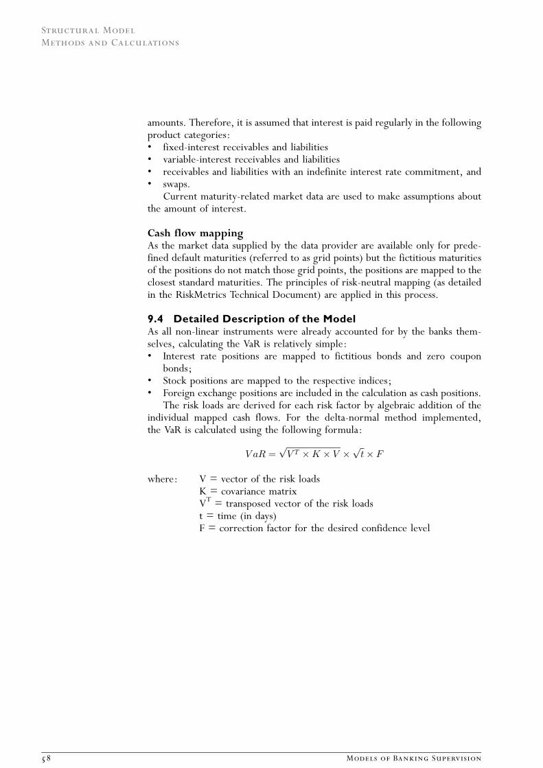
amounts. Therefore, it is assumed that interest is paid regularly in the followingproduct categories:¥ fixed-interest receivables and liabilities¥ variable-interest receivables and liabilities¥ receivables and liabilities with an indefinite interest rate commitment, and¥ swaps.

Current maturity-related market data are used to make assumptions aboutthe amount of interest.

Cash flow mappingAs the market data supplied by the data provider are available only for prede-fined default maturities (referred to as grid points) but the fictitious maturitiesof the positions do not match those grid points, the positions are mapped to theclosest standard maturities. The principles of risk-neutral mapping (as detailedin the RiskMetrics Technical Document) are applied in this process.

9.4 Detailed Description of the ModelAs all non-linear instruments were already accounted for by the banks them-selves, calculating the VaR is relatively simple:¥ Interest rate positions are mapped to fictitious bonds and zero coupon

bonds;¥ Stock positions are mapped to the respective indices;¥ Foreign exchange positions are included in the calculation as cash positions.

The risk loads are derived for each risk factor by algebraic addition of theindividual mapped cash flows. For the delta-normal method implemented,the VaR is calculated using the following formula:

V aR ¼ffiffiffiffiffiffiffiffiffiffiffiffiffiffiffiffiffiffiffiffiffiffiffiffiffiffiV T �K � V

p�

ffiffit

p� F

where: V = vector of the risk loadsK = covariance matrixVT = transposed vector of the risk loadst = time (in days)F = correction factor for the desired confidence level

Structural Model



V is an ðm� 1Þvector

1:::m

��

��; V T is a ð1�mÞvector : 1. . .m

K is an ðm�mÞmatrix

1 . . . 1m. .. .. .

m1 . . . mm

��

��:

Details about these calculations can be found in the RiskMetrics TechnicalDocument.

9.4.1 Calculating the Incremental VaRThe procedure used to calculate VaR shows that Value at Risk is not additive,neither in terms of risk factors nor in terms of assets. This additivity would onlyexist given a perfectly positive correlation (i.e. with all correlation coefficientsequaling one). In any other case, the VaR of a portfolio is smaller than the sumof the VaRs of the individual portfolio assets.

This lack of additivity in the VaR indicator led to the definition of incremen-tal Value at Risk. The incremental VaR of a securities position is that contribu-tion to VaR made by this position in the context of the portfolio. Formally, thisis expressed by deriving VaR for the risk weight fi (incremental VaR of a riskfactor) or the asset weight wk (incremental VaR of an asset) multiplied by thespecific weight value: incremental VaR of the risk factor:RI

incV aRRi¼ �V aRp

�fifi ¼ V aRp

�ðRi; PRÞ�2ðPRÞ

fi

incremental VaR of Asset Ak:

incV aRAk¼ �V aRp

�wkwk

10 Operational RiskThe next section presents the methods of calculating operational risk underBasel II, the calculation in our structural model, and the weaknesses of theselected approach.

10.1 Significance of Operational RiskBasel II defines operational risk as the �risk of loss resulting from inadequate orfailed internal processes, people and systems or from external events. Thisdefinition includes legal risk, but excludes strategic and reputational risk.�

Structural Model



This type is a major source of risk for banks, as we have seen in internationalstudies which break the results of various banks� economic capital models downinto their various risk components. According to these studies, a significantportion of economic capital is determined by operational risk, an assertionwhich also appears to be true in Austria. Furthermore, losses from operationalrisk events have been the cause of bank failures in many cases, both domesticallyand internationally.12

Operational risk is thus a factor which cannot be ignored for the purposes ofbanking supervision in general and off-site analysis in particular, and it should bemeasured and evaluated for all banks in the future.

10.2 Basel II and the Determination of Operational RiskIn its new regulatory framework, the Basel II committee has also acknowledgedthe importance of operational risk and therefore included it in their consider-ations. On the one hand, Basel II provides for a regulatory capital requirementfor operational risk, which can be calculated using at least three differentapproaches. On the other hand, the second pillar explicitly calls upon banksto set up adequate risk management processes which can be used to measureand reduce material operational risk exposure and to take precautions to ensurecontinued operations in the event of operational losses.

However, we will demonstrate below that the rather simple approaches incurrent Basel II regulations — which are likely to be applied by most banks —do not measure actual operational risk adequately.

10.2.1 Basic Indicator ApproachIn the simplest of all approaches, the capital requirement is calculated as a fixedpercentage (15%) of the bank�s gross income. This approach is based on thenotion that higher gross incomes are usually linked with higher operational risksand may thus serve as a very rough approximation of operational risk. However,there are serious doubts as to the risk sensitivity of this approach, which rendersit rather unsuitable for off-site analyses in the long run.

10.2.2 Standardized ApproachUnder the standardized approach, the bank�s activities are divided into eightstandard business lines, and the average gross income is calculated for eachbusiness line over the three previous years. Each of these amounts is multipliedby a different beta factor (12-18%), with the sum of these amounts equaling thecapital requirement. The standardized approach assumes different risk situationsin the various business lines of a bank. For example, it is assumed that retailbanking is subject to a lower level of operational risk than corporate finance;this assumption is reflected in different factors. While the standardizedapproach certainly reflects a bank�s operational risk better than the basicindicator approach does, the basic assumption that it is possible to captureoperational risk using gross income remains doubtful.

A number of qualitative criteria have to be met in order for a bank to receiveapproval for a standardized approach. Among other things, banks are required

12 e.g. Deutsche Morgan Grenfell (1996); BankersTrust (1994-1998); Barings Bank (1995).

Structural Model



to establish a loss database, a working operational risk management mechanismwhich is integrated into operations, suitable reporting, documentation, andinternal as well as external validation of the systems.

10.2.3 Advanced Measurement ApproachesWhen it comes to advanced measurement approaches, banks enjoy a largedegree of discretion. One of the objectives is, for example, to determine abank�s actual operational risk based on historical experience. According to cal-culations using the loss database, those losses which will not be exceeded withinone year with a probability of 99.9% are to be covered by equity. In addition tothis high quantitative threshold, which means that higher losses from operationalrisk events may be expected only once in 1,000 years (or for one in 1,000banks), banks are also required to meet comprehensive qualitative criteria.Among other things, banks have to establish an independent, conceptuallysound and extensively documented risk management system whose regularreports to business line managers, the supervisory board and managementboard have an impact on risk management and reduction.

Advanced measurement approaches are certainly best able to determineactual operational risks. However, the high quantitative and qualitative require-ments make it doubtful from today�s perspective that the investment in devel-oping an advanced equity-based approach will pay off for smaller banks.

Neither the Basel nor the Brussels Consultation Paper states specificrequirements as to the way in which such measurement approaches are to bedesigned. However, the Basel Committee�s �Working Paper on the RegulatoryTreatment of Operational Risk� outlines three methods which are being appliedin practice with increasing frequency:

Internal ratings-based approachesThese approaches assume a fixed relation between the expected loss (as theexpected value of the loss distribution) and the value at the corresponding con-fidence level. This allows a rather simple calculation of the capital requirementfor each combination of risk type and business line, as the relation betweenexpected value and extreme events has to be determined only once and can thenbe assumed to be constant.

Loss distribution approachesUnder loss distribution approaches, the distribution of operational losses is esti-mated for each combination of risk type and business line, then the correspond-ing confidence level for each of these distributions is assumed in order to deter-mine the capital requirement. As a rule, two separate distributions are assumedin each combination of risk event and business line, for example a Poisson or ageometric distribution for the number of losses, and a log-normal or an expo-nential distribution for the amount of losses. The VaRs resulting from thesecombinations can then simply be added up or aggregated using an assumed cor-relation matrix.

Structural Model



Scorecard approachesIn scorecard approaches, the capital requirement is determined for operationalrisk and then modified by a qualitative forecast of operational risks in the indi-vidual business lines. However, such scorecard approaches need to be suffi-ciently substantiated on a quantitative basis and validated by historical data.In general, scorecards can capture operational risks in quite some detail andfrom an anticipatory perspective, while quantification using a potential amountof loss at a given confidence level proves to be more difficult.

No industry standard has been established to date, but many medium-sizedand large banks are setting up loss databases to make it possible to quantifyoperational risk as well as developing scorecards to capture, manage, and limitoperational risk more effectively. What all approaches have in common is thatboth obtaining the necessary data and applying them in a methodically correctmanner often cause problems in practice.

However, advanced measurement approaches generally reflect operationalrisk appropriately, which does make it possible to use the resulting findingsin off-site analyses. Due to the relatively high demands on systems and risk man-agement, however, we cannot expect a large number of Austrian banks to con-sider developing advanced approaches in the near future.

10.3 Selected ProcedureDue to the lack of a complete database, Austria�s regulators currently have onlylimited means of capturing operational risk comprehensively and, in particular,quantifying operational risk through off-site analysis.

Until it is possible to determine operational risk in a theoretically soundmanner by qualitative recording and quantification using a loss database, the lossdistribution for operational risk is determined as follows:1. An indicator for KBasel II operational risk is defined using the basic indicator

approach under Basel II.2. We assume a geometric distribution with the parameter p for the actual

distribution:

fðnÞ ¼ pð1� pÞn�1 EðNÞ ¼ p; StdðNÞ ¼ 1� p

p2

3. We assume an exponential distribution with the parameter ...� for theamount of losses:

gðxÞ ¼ ��x EðXÞ ¼ StdðXÞ ¼ �

4. For the loss distribution, this yields Sn ¼Pn

i¼1Xi

P ðS sÞ ¼X1n¼1

P ðSn s j nÞfðnÞ

Structural Model



5. However, as the sum of identical independently distributed random varia-bles follows a gamma distribution, the distribution function is defined by

P ðSn s j nÞ ¼Z s

0

1

ðn� 1Þ!�nun�1e��udu

6. Or, after solution of the equation:

P ðS sÞ ¼ 1� e��ps

7. This means, however, that the losses from operational risk again follow anexponential distribution with only one parameter � ¼ ��p:

hðsÞ ¼ ð�pÞe�ð�pÞs

8. This also means the VaR for operational risk at confidence level c is clearlydefined by:

EðSÞ � s� ¼ 1

�

� �½lnð1� cÞ þ 1�

9. If we then interpret the indicator KBasel II found in Item 1 as a VaR for acertain confidence level, we can estimate the missing parameter � and thusthe entire loss distribution for operational risk. This also makes it possible tocalculate the VaR for other confidence levels and to perform aggregationwith the other types of risks.The advanced Basel II approaches calculate the capital requirement as the

99.9% confidence level for expected and unexpected losses. If we assume thata calibration to these values was also used for the simpler approaches, they couldbe used to approximate and estimate the parameter �:

KBasel II ¼1

�

� �½lnð1� 0; 999Þ þ 1�

However, banks have indicated that the results for the equity requirement areclearly different under the advanced measurement approaches compared tothe simpler approaches, as the capital requirement found using advancedapproaches is sometimes considerably higher than in the simpler approaches.Thus, there is also the possibility of determining the confidence level impliedin the simpler approaches from the calculations of those banks which are alreadyin a position to use simple as well as advanced calculation methods foroperational risk.

However, in order to ensure methodical consistency with the supervisoryregulations in Basel II, the confidence level applied there is still used, even ifthis might lead to underestimates of actual operational risk. The actualimplementation in calculating the model, however, allows flexibility inmodifying this assumption.

Structural Model



The database used for the procedure described above is gross incomeaccording to the stated definition. These data are already available in theAustrian reporting system, thus it possible to calculate the corresponding valueas the average over the last three years.

Subsequently, it was possible to calculate the indicator in accordance withthe Basel method using the the moving values as a basis. Based on the processmentioned above, it was possible to determine the factor of the exponentialdistribution (formula: — (LN(1-confidence level)+1)/capital requirement).The loss distribution assumed for operational risk is already defined completelyby this factor.

Calculation of VaR for operational riskIt is then easy to compute V aROp

� by generating the respective confidence levelsof the exponential distribution, a procedure which also ensures aggregabilitywith the other risks.

11Capacity to Cover LossesAs a framework for risk management, risk-bearing capacity forms an importantbasis for management control in banking. It is essential to identify in this respectthe extent to which a bank can afford to assume risks.

In general, equity capital serves to cover potential risks; depending on theperspective chosen, one can look at the book value or the net asset value ofequity, or use the regulatory definition of capital. The latter definition,however, allows for example hidden reserves only to a limited extent, althoughthey might well be used as potential cover in an internal calculation. As thereare other items besides regulatory capital that may be used as coverage capital, itseems appropriate to classify risk coverage capital into different categories.

This gives rise to the following questions concerning risk-bearing capacityfor regulatory analysis:1. What do the capacities to cover expected losses, the changes and level of

provisions, and the profitability look like?2. What do the capital requirements for solvency look like?3. What does the coverage of expected and unexpected losses from an eco-

nomic point of view look like?The next section shows how and to what extent the capacities to cover

incurred risks were defined in the structural model.

11.1 Classification of Risk Coverage CapitalUsing a classification of the reserves, i.e. the capacity to cover losses, makes itpossible13 to allow for the fact that risks have different probabilities on the onehand, while the availability of financial resources varies strongly on the other.

Level 1 reserves: internal provisionsIt is not clear whether it is permissible to cover expected losses in the calcula-tion of risk-bearing capacity, as these losses are actually a cost factor which

13 The definition is based on Schierenbeck (2002).

Structural Model



should be included as standard risk costs. Therefore, they are not a risk in thetechnical sense, as risks are usually defined as potential negative deviations fromthe expected result. However, they are listed here for the sake of completeness.

Should losses be realized within expectations, the first measure is to reversethe precautionary measures taken in terms of provisions and risk costs. Next,any profit exceeding expectations can be reduced. The expected minimumprofit on paid-in capital, however, is only counted as part of level 3 reserves.

Profits and losses brought forward from previous years also have to be takeninto account as additional, easily available risk provisions in the case of profitsand as deductible items in the case of losses.

Level 2 reserves: accounting surplusesShould the incurred losses exceed expectations, it will be necessary to reducehidden reserves to cover these losses. However, only those parts which do notrepresent tier 2 capital are treated as level 2 reserves. These hidden reservesarise in connection with securities, investments, and property, as well as excessrisk or pension provisions.

The extent of the level 2 reserves to cover risk is certainly a major factor inrisk coverage capital and thus needs to be assessed carefully in order to ensurethe model�s goodness of fit.

Especially level 1 (but also level 2) reserves may be used without attractingpublicity, while this is hardly possible in the case of higher level loss coverage.

Level 3 reserves: easily available own fundsOnce hidden reserves have been exhausted, it is possible to absorb further lossesby reducing or suspending the payout of dividends to the owners.

It is also possible to make use of the fund for general bank risks, which isalready part of tier 1 capital. This fund comprises provisions which the creditinstitution considers necessary to cover special banking risks and thus the accessto them must be unrestricted and immediate

Any excess of own funds above the legally mandated minimum should alsohave to be considered part of the level 3 reserves, as it could be used in the caseof losses without affecting the bank�s solvency.

In general, the level 1 to 3 reserves are intended to cover exceptionalnegative events without threatening the bank�s existence. However, as soon asa bank has used up its excess equity, it is likely that regulatory measures willbe taken.

Level 4 reserves: further coverage by owners (tier 1)Should it prove necessary to tap level 4 reserves to cover a loss, this will cut intocore balance sheet capital. Disclosed reserves and payed-up capital will be usedup first, as these represent the equity which best meets the requirements ofoffsetting losses and which can be accessed by the credit institutions withoutrestrictions at any time.

50% of the excess equity determined as part of the primary reserves has tobe deducted. This split can be explained by the fact that subordinated capital canonly be applied up to the level of tier 1 capital, which means that both positionswould have to be reduced almost to the same extent if reserves are reversed.

Structural Model



Should realized losses not exceed the level 4 reserves, this would result indefault without harming clients or requiring the intervention of a deposit insur-ance organization.

Level 5 reserves: Capacity to cover losses:coverage by investors (tier 2 + 3)Only in extreme emergencies will the banks tap subordinated capital compo-nents. In many cases, such capital components are no longer included as riskcover in internal calculations, as — by definition — the non-repayment of subor-dinated capital already has to be classified as default in the broad sense of theterm.

Level 5 risk cover consists of the sum of the tier 2 components (certain pre-defined hidden reserves, supplementary capital, participation capital, revalua-tion reserves, and the liability sum surcharge, i.e. additional cover by cooper-ative members) and tier 3 capital. Note that the available components — not theeligible or regulatory components — have to be included in this context.Exhausting quintary reserves ultimately leads to the bank�s insolvency, butdeposits should not yet be endangered at this stage. Bondholders, on the otherhand, would already lose their capital in this case.

Should realized losses also exceed the level 5 reserves, however, this wouldresult in a default, which would harm depositors and require the intervention ofa deposit insurance organization.

Furthermore, when looking at the capacities to cover losses it must be notedthat sector peculiarities such as �Besserungsgeld� (specific internal short-termliabilities) or intervention on the part of a solidarity fund are not taken intoaccount at this stage.

Structural Model



11.2 Capacity to Cover LossesThe table below shows the relative composition of the capacities to cover lossesin the two examples.

Clear differences also become evident in this case, especially if the tertiarycapacity to cover losses is defined as the boundary between default and non-default. While Bank A has more than half of its cover in the tertiary reservesand can access these funds quite easily, the corresponding figure for Bank B isonly one third. A substantial part of Bank B�s capacity to cover losses resultsfrom available equity, which should only be used to cover losses in emergencies.

12 Assessment of Total RiskAfter calculating the total bank VaRs for different confidence levels andcalculating the various reserves, the next and final step is to combine thesetwo components.

Following the explanations above, it is now necessary to determine the fullloss distributions of the three types of risk described in order to calculate thebank�s overall loss distribution. This is done by adding up the respective VaRsat the same confidence level.

This does not present a problem for credit, market, and operational risk, asthe methods stated yield the complete loss distribution anyway. The VaRs can beevaluated for each predefined confidence level, and the expected loss can becalculated for all types of risks. Due to our assumption of normal distribution,the expected loss of market risk is always assumed to be zero.

�� '��,��+�� ( ��(,��0��+�� ( � ('��-�� ( ��(��-��1�� *( �*(��!��+�� ( ��(��+� ��( � (�� *( ,�(��+�� ( �*(!��!�!�� ( ��(�� *( �*('��"�� ( �*(��+�� ( (��+� ��( *(�� ( ��(��!�� *( ,�(��*%��'��"��$��& ,�( ,�("��+�� ( � (��!�� ( ��(�� ( � (��*%��'��"��$��& ,�( ,�("��+�� **( �**(

Structural Model



12.1 Theoretical BackgroundAggregating the individual risks leads to a total VaR. This value shows that thesum of the losses from the three risk categories (market, credit, and operationalrisk) will not exceed this level within a year with a probability of �. From theregulatory perspective, this information concerning the absolute VaR is notparticularly important. Instead, the total VaR becomes an indicator if thechanges in value over time are observed (i.e. if the extent to which the VaRhas changed upward or downward is recorded); alternatively if the economiccapital determined using the VaR is related to the coverage capital. Let usassume that a bank�s coverage capital is equal to D. We find the significance levelfor which

V aRtotalð�Þ �D ¼ 0

One minus that significance level for which the total VaR equals the availablecoverage capital D is the bank�s probability of default as determined by themodel. The graph below illustrates this link. The y-axis of the graph showsthe total VaR assigned to a certain significance level, while the x-axis showsthe significance level. The curve, which is similar to a section of a hyperbola,shows the relation between the significance level and VaR. If the distributionsof the individual loss categories have a support of ð�1;1Þ;, then the curvemust approach the two axes asymptotically. If we now include the bank�scoverage capital in the graph, we can immediately read the probability ofdefault.

12.2 Derivation of Implied Default ProbabilitiesUsing the approaches suggested, it is possible to compare the loss distributionwith the various reserves with due attention to the quality of the capitalemployed to cover losses. The first step usually consists in using the reservesfor potential losses or any excess profit. Subsequently, hidden reserves are used,

��.�� /��

�� +��

��+��

��+��

Structural Model



or the fund for general bank risks may be tapped. Only once these sources havebeen exhausted will subscribed capital or disclosed reserves be utilized. Subor-dinated capital components (for more details on the capacity to cover losses seesection 11) are touched only in extreme cases. Such hierarchy would allowseveral intuitively understandable interpretations.

The recommended calculation of the various default probabilities can beimplemented directly based on the resulting values by tracing those VaRs inthe loss distribution for the bank as a whole which exactly match the respectivereserves. By definition, one minus the confidence level implied by the VaR is thecorresponding default probability.

This approach can now be illustrated for our two sample banks:

Interestingly, both banks show a high probability that the expected losseswill exceed primary reserves. While the default probability is low for bothinstitutions, there is a relatively higher risk for Bank B.

12.3 Reviewing Adherence to Coverage ConditionsThe coverage conditions described in section11 can also be checked directly bymeans of the resulting total bank loss distribution and the reserves.

For this purpose, the following three loss events are defined and comparedto the respective reserves:1. Normal case: based on expected loss;2. Negative case: based on a realization of losses at a confidence level of 95%;3. Worst case: based on a realization of losses at a confidence level of 99.9%.

��'��+��1��1��+��1��'�� / *( / *(

��!��"��$'��"��&��+��)1��'�� %�*( %**(

��!��"��+��)�1��'��2��%%��1��!��!�� 1�� *%*�( *% *(

��3��"��$��4��&��+��)��%%�� !��!��"�� *%*�( *%*�(

��

Structural Model



The results can be illustrated nicely by a traffic light:

In our case, while the bank appears to have sufficient resources to cover eventhe worst case losses, the provisions for expected losses are insufficient.

13SummarySince the fundamental goal is to develop a model for evaluating all banksoperating in Austria, numerous assumptions had to be made in calculatingeconomic capital.

For credit risk, we can see that the current reporting system (especially forloans below the Major Loans Register limit of EUR 350,000) allows only lim-ited conclusions as to the actual risk in this area, and that rating information inMajor Loans Register is only available from 2003 onward.

Similarly, market risk is integrated into the structural model in order to offera coherent and comprehensive view of risk and to provide information on theextent of market risk and its contribution to total risk. Well-known andestablished industry standards for the quantitative measurement of market riskhave existed for some time, so that the concept�s implementation in regulatoryactivities will hardly cause any problems from a theoretical point of view.However, the Austrian regulatory authorities are well aware that given thenature of the current reporting data the VaR calculated in the structural modelcan only be an approximation. Nevertheless, this approximation appears to besufficiently realistic for use in supervisory risk assessment and thus represents anappropriate tool within total risk analysis.

The weaknesses resulting from using gross income as an indicator in meas-uring operational risk have already been dealt with in detail. Similarly, theassumption that the capital requirement under Basel II corresponds to a VaRat a certain confidence level seems questionable. It must be noted that theregulators need new data on operational events in order to determineoperational risk accurately, as otherwise the required risk sensitivity is notensured.

In the first step, a pragmatic but reasonable approach to aggregate the riskswas chosen, and this approach will certainly be refined in the coming years. Inthis context, it will be necessary to intensify our exchange of knowledge andexperience with the banks, which currently face similar problems.

In spite of this less than optimal starting point, we have been able to developa model which — based on numerous plausibility checks and consultations withexperts — can be considered highly effective tool for bank risk analysis. The

5�� '��

6��!��+�

��+��6

��!��+��1��

6��!��"��+�

��1� *(

��1� *(#�%**(

#�%�*(/##%#*(

/##%##(

'��

��+��

��+��

Structural Model



FMA and the OeNB are convinced that these models bring Austrian bankingsupervision to a level comparable with the best European and internationalstandards.

Structural Model



A n n e x

14 List of Figures

Figure 1: Data sources used 15Figure 2: The ROC Model 19Figure 3: Development of the PDs for different approaches 22Figure 4: Survival Curves in the Cox Model 26Figure 5: Composition by type of risk 38Figure 6: Credit loss distribution of an Austrian credit institution 39Figure 7: Default probabilities of industry groups 43Figure 8: Dependence of credit VaR on the number of bands chosen 47Figure 9: Scenario analysis 51Figure 10: VaR for market risk 54Figure 11: Data preparation for market risk 56Figure 12: Economic capital vs. coverage capital 68

Annex


15 References

Statistical ModelAltman. E.I. 1968. Financial Indicators, Discriminant Analysis, and the Prediction of Corporate Bankruptcy,

Journal of Finance.

Barniv, R., A. Agarwal, and R. Leach. 1997. Predicting the Outcome Following Bankruptcy Filing:

A Three-State Classification Using Neural Networks, International Journal of Intelligent Systems in

Accounting, Finance and Management 6.

Boss, M. 2002. Ein makroo‹konomisches Kreditrisikomodell zur Durchfu‹hrung von Krisentests fu‹r das

o‹sterreichische Kreditportfolio, Finanzmarktstabilita‹tsbericht 4.

Charitou, A., and C. Charalambous. 1996. The Prediction of Earnings Using Fi-nancial Statement

Information: Empirical Evidence with Logit Models and Artificial Neural Networks, Journal of Intelligent

Systems in Accounting, Finance and Management 5.

Cox, D. R., Regression Models and life tables (with discussion), Journal of Royal Statistical Society, Series B.

Cox, D. R., and D. Oakes. 1984. Analysis of Survival Data, Chapman Hall, London.

Davidson, R., and J. G. MacKinnon. 1993. Estimation and Inference in Econometrics, Oxford.

Engelmann, B., Hayden, E., and D. Tasche. 2003. Testing Rating Accuracy, Risk.

Henebry, K. L. 1996. Do Cash Flow Variables Improve the Predictive Accuracy of a Cox Proportional

Hazards Model for Bank Failure?, The Quarterly Review of Economics and Finance, Vol. 36 (3).

Hodrick, R., and C. Prescott 1997. Post-War U.S. Business Cycles: An Empirical Investigation, Journal of

Money, Credit and Banking 29.

Hosmer, D., and S. Lemenshow. 1989. Applied Logistic Regression, JohnWiley & 38; Sons.

Hosmer, D., and S. Lemenshow. 1999. Applied Survival Analysis, JohnWiley & 38; Sons.

Kalirai, H., Scheicher, M. 2002. Makroo‹konomische Krisentests: Erste Ergebnisse fu‹r O‹ sterreich,

Finanzmarktstabilita‹tsbericht 3.

Lawless, J. F. 1982. Statistical Models and Methods for Lifetime Data, John Wiley & 38; Sons, New York.

Maddala, G. S. 1983 Limited-Dependent and Qualitative Variables in Econometrics, Econometric Society

Monographs, Cambridge University Press.

Turner, J. 2000. The Austrian Supervisory Risk Assessment System, Focus on Austria 1, Oesterreichische

Nationalbank.

Whalen, G. 1991. A Proportional Hazard Model of Bank Failure: An examination of its usefulness as an

early warning tool, Federal Reserve Bank of Cleveland, Economic Review, 1st Quarter.

Structural ModelBu‹hler, W., Engel, C., Stahl, G. 2002. Backtesting von Kreditrisikomodellen [Backtesting Credit Risk

Models], in: Oehler, A. (Ed.), Kreditrisikomanagement: Kernbereiche, Aufsicht und Entwicklungsten-

denzen, Scha‹ffer-Poeschel, Stuttgart.

Credit Suisse Financial Products. 1997. CreditRisk+, A Credit Risk Management Framework.

CreditMetricsTM. 1997. Technical Document, RiskMetrics Group.

Culp, C. 2001. The Risk Management Process: Business Strategy and Tactics, John Wiley & 38; Sons.

Embrechts, P., Ho‹ ing, A. and Juri, A. 2001. Using Copulae to bound the Value-at-Risk for functions of

dependent risks, Finance and Stochastics.

Esterella, A. 2000. Cost and benefits of mandatory subordinated debt regulation for banks, Federal

Reserve Bank of New York.

Evanoff, D. D., Wall, L. D. 2002. Measures of the riskiness of banking organizations: subordinated debt

yields, risk-based capital, and examination ratings, Journal of Banking and Finance.

Evanoff, D. D., Wall, L.D. 2003. Subordinated debt and prompt corrective regulatory action, Federal

Reserve Bank of Chicago.

References


Giese G. 2003. Enhancing CreditRisk+, Risk, Vol.16, No. 4.

Gordy M. 1998. A Comparative Anatomy of Credit Risk Models.

Gordy M. 2002. Saddlepoint Approximation of CreditRisk+, Journal of Banking and Finance, Vol. 26, No 7.

Gropp, R., Vesala, J., Vulpes, G. 2002. Equity and Bond Market Signals as Leading Indicators of Bank

Fragility, ECB Working Paper Series, 150.

Haaf H., Rei§ O., Schoenmakers J. 2003.Weierstra§-Institut fu‹r Angewandte Analysis und Stochastik:

Numerically Stable Computation of CreditRisk+.

Hiwatashi, J. 2002. Solutions on measuring operational risk, Capital Market News, Federal Reserve Bank

of Chicago.

J. P. Morgan, Risk Metrics TM, technical document, fourth edition, 1996.

Kretschmer J. 1999. CreditRisk+, Ein portfolioorientiertes Kreditrisikomodell, aus Handbuch Kreditrisiko-

modelle und Kreditderivate, R. Eller, W. Gruber, M. Reif (Eds.), Scha‹ffer-Poeschel Verlag.

Kuritzkes, A., Schuermann, T., Weiner, S. 2002. Risk Measurement, Risk Management, and Capital

Adequacy in Financial Conglomerates, Wharton Working Paper Series 03—02.

Matten, C. 2000. Managing Bank Capital, Wiley & 38; Sons, 2nd Edition.

Nelsen, R. 2002. An Introduction to Copulas, Springer Verlag New York.

Netter, J. M., Poulsen, A. B. 2002. Operational Risk in Financial Service Providers and the Proposed

Basel Capital Accord: An Overview, University of Georgia, Working Paper.

Schierenbeck, Henner. 2003. Vol. 1: Grundlagen, Marktzinsmethode und Rentabilita‹ts-Controlling,

Gabler Verlag.

Schierenbeck, Henner. 2003. Vol. 2: Risiko-Controlling und integrierte Rendite-/Risikosteuerung,

Gabler Verlag.

U.S. Shadow Regulatory Committee. 2000. Reforming bank capital regulation, The AEI Press:

Washington D.C.

References


new quantitative models of banking supervision - …df69f8e1-ebcb-4fcf-8a60-5bb8b3f48223/... · the...

Documents