Astronomy&Astrophysics

A&A 632, A126 (2019)https://doi.org/10.1051/0004-6361/201936580© ESO 2019

New predictions for radiation-driven, steady-state mass-loss andwind-momentum from hot, massive stars

I. Method and first results

J. O. Sundqvist1,3, R. Björklund1, J. Puls2, and F. Najarro3

1 KU Leuven, Instituut voor Sterrenkunde, Celestijnenlaan 200D, 3001 Leuven, Belgiume-mail: jon.sundqvist@kuleuven.be

2 LMU München, Universitätssternwarte, Scheinerstr. 1, 81679 München, Germany3 Centro de Astrobiologia, Instituto Nacional de Tecnica Aerospacial, 28850 Torrejon de Ardoz, Madrid, Spain

Received 27 August 2019 / Accepted 11 October 2019

ABSTRACT

Context. Radiation-driven mass loss plays a key role in the life cycles of massive stars. However, basic predictions of such mass lossstill suffer from significant quantitative uncertainties.Aims. We develop new radiation-driven, steady-state wind models for massive stars with hot surfaces, suitable for quantitative predic-tions of global parameters like mass-loss and wind-momentum rates.Methods. The simulations presented here are based on a self-consistent, iterative grid solution to the spherically symmetric, steady-state equation of motion, using full non-local thermodynamic equilibrium radiative transfer solutions in the co-moving frame to derivethe radiative acceleration. We do not rely on any distribution functions or parametrization for computation of the line force responsiblefor the wind driving. The models start deep in the subsonic and optically thick atmosphere and extend up to a large radius at which theterminal wind speed has been reached.Results. In this first paper, we present models representing two prototypical O-stars in the Galaxy, one with a higher stellar massM∗/M� = 59 and luminosity log10 L∗/L� = 5.87 (spectroscopically an early O supergiant) and one with a lower M∗/M� = 27 andlog10 L∗/L� = 5.1 (a late O dwarf). For these simulations, basic predictions for global mass-loss rates, velocity laws, and wind momen-tum are given, and the influence from additional parameters like wind clumping and microturbulent speeds is discussed. A key resultis that although our mass-loss rates agree rather well with alternative models using co-moving frame radiative transfer, they are signif-icantly lower than those predicted by the mass-loss recipes normally included in models of massive-star evolution.Conclusions. Our results support previous suggestions that Galactic O-star mass-loss rates may be overestimated in present-day stellarevolution models, and that new rates might therefore be needed. Indeed, future papers in this series will incorporate our new modelsinto such simulations of stellar evolution, extending the very first simulations presented here toward larger grids covering a range ofmetallicities, B supergiants across the bistability jump, and possibly also Wolf-Rayet stars.

Key words. radiation: dynamics – radiative transfer – hydrodynamics – stars: massive – stars: mass-loss – stars: winds, outflows

1. Introduction

For hot, massive stars of spectral type OB, scattering andabsorption in spectral lines transfer momentum from the intenseradiation field of the star to the plasma, thereby providing theforce necessary to overcome gravity and drive a stellar wind out-flow (Lucy & Solomon 1970; Castor et al. 1975; review by Pulset al. 2008). The line-driven winds of OB stars are very strongand fast, exhibiting mass-loss rates M ∼ 10−5···−9 M� yr−1 and ter-minal wind speeds 3∞ that can reach several thousand kilometersper second. Furthermore, since the radiation acceleration graddriving these outflows is dominated by lines from metal ions likeFe, C, N, O, and so on, the winds are predicted and are shownto depend significantly on stellar metallicity Z? (e.g., Kudritzkiet al. 1987; Vink et al. 2001; Mokiem et al. 2007).

The first quantitative description of such line-driven windswas given in the seminal paper by Castor et al. (1975; referred tohereafter as CAK). Using the so-called Sobolev approximation1

1 The Sobolev approximation assumes number densities and sourcefunctions are constant over a few Sobolev lengths LSob = 3th/(d3s/ds)in direction s for ion thermal speed 3th. This then allows for a localtreatment of the radiative line transfer.

in combination with an assumed power-law distribution ofspectral line-strengths, CAK estimated the total line force,derived a parameterization for grad, and developed a wind-theorythat provided very useful scaling relations of M and 3∞ withfundamental parameters like stellar luminosity L? and mass M?.

Extensions of this elegant theory (Pauldrach et al. 1986;Friend & Abbott 1986) have had considerable success in explain-ing many basic features of stellar winds from OB stars. However,over the years evidence has accumulated that such modelsmay not be able to make quantitative predictions with therequired accuracy. Namely, although CAK-type and Sobolev-based Monte-Carlo line-transfer models typically agree ratherwell on predicted M (Pauldrach et al. 2001; Vink et al. 2000,2001), more recent simulations based on line radiation transferperformed in the co-moving frame (CMF), or by means of a non-Sobolev Monte-Carlo line force, seem to suggest overall lowerrates (Lucy 2007, 2010; Krticka & Kubát 2010, 2017; Sanderet al. 2017). Moreover, although the studies above, as well asthis paper, focus solely on the global, steady-state wind, sometime-dependent models with grad computed in the frame of theobserver also indicate similar mass loss reductions as comparedto CAK-based simulations (Owocki & Puls 1999).

Article published by EDP Sciences A126, page 1 of 13

A&A 632, A126 (2019)

Concerning attempts to derive M directly from observationsof stellar spectra, a multitude of results are scattered throughoutthe literature. One key uncertainty is in regards to the effects ofa clumped wind, which if neglected in the analysis may lead torates that differ by large factors for the same star, depending onwhich spectral diagnostic is used to estimate M (Fullerton et al.2006). When accounting properly for such “wind clumping”,including the light-leakage effects of porosity in physical andvelocity space, a few first multiwavelength studies of GalacticO-stars (Sundqvist et al. 2011; Šurlan et al. 2013; Shenaret al. 2015) suggest mass-loss rates that are lower than orapproximately equal to those predicted by the Vink et al. (2000)standard mass-loss recipe. These results also agree well withX-ray (Cohen et al. 2014) and infra-red (Najarro et al. 2011)studies, as well as with the analysis by Puls et al. (2006) thatderived upper limits on M by considering diagnostics rangingfrom the optical to radio. On the other hand, some extragalacticstudies (Ramírez-Agudelo et al. 2017; Massa et al. 2017) findupper M limits that typically are higher than the Vink et al.(2000, 2001) recipe. Clearly, more effort will be needed here inorder to place better observational constraints on the mass-lossrates from hot, massive stars.

Reduced mass-loss rates could further have quite dramaticconsequences for model predictions of stellar evolution and feed-back (e.g., Smith 2014; Keszthelyi et al. 2017). Indeed, thepresence of mass loss has a deciding impact on the lives anddeaths of massive stars, affecting their luminosities, chemicalsurface abundances, rotational velocities, and nuclear burninglifetimes, as well as ultimately determining which type of super-nova the star explodes as and which type of remnant it leavesbehind (Meynet et al. 1994; Langer 2012; Smith 2014). Assuch, a key aim of this series of papers is – in addition toproviding new quantitative predictions of mass loss – to incor-porate our new models directly into simulations of massive-starevolution.

In this first paper, we outline the basic methods of our newwind simulations, which were computed using steady-statehydrodynamics and non-local thermodynamic equilibrium(NLTE)2 CMF radiative transfer calculations within thecomputer-code network FASTWIND (Santolaya-Rey et al. 1997;Puls et al. 2005; Carneiro et al. 2016; Puls 2017; Sundqvist &Puls 2018). Moreover, we present and discuss some first resultsfrom two selected models of O-stars in the Galaxy. The secondpaper will present results from a larger grid of such O-starsimulations, covering metallicities of the Galaxy and theMagellanic Clouds (Björklund et al., in prep.). The third paperwill then extend these calculations to B-stars, examining inparticular mass-loss and wind-momentum properties over theso-called bistability jump (where iron recombines from beingthree to two times ionized, thus providing many more drivinglines, Pauldrach & Puls 1990; Vink et al. 2000). In a fourthpaper we will fully incorporate our predictions into models ofstellar evolution, and carefully investigate the correspondingeffects (Björklund et al., in prep.). Further follow-up studies willthen focus on, for example, time-dependent effects and wind-clumping (see also Sect. 4.3) and potentially even an extensionof our current models to the highly evolved, classical Wolf-Rayetstars whose supersonic winds are optically thick also for opticalcontinuum light.

2 NLTE here means number densities computed assuming statisticalequilibrium (see book by Hubeny & Mihalas 2014 for an extensiveoverview).

2. Basic equations and assumptions

Global models (containing both the subsonic stellar photosphereand the supersonic wind outflow) are computed by a numerical,iterative grid-solution to the steady-state (time-independent)radiation-hydrodynamical conservation equations of mass andmomentum in spherical symmetry. These are supplemented byalso considering the energy balance, either by a method basedon flux-conservation and the thermal balance of electrons (Pulset al. 2005) or by a simplified temperature structure derived fromflux-weighted mean opacities in a spherical, diluted envelope(Lucy 1971).

For gravitational acceleration g(r) and (isothermal) soundspeed

a2(r) =kbT (r)µ(r)mh

, (1)

where T (r) is the temperature, µ(r) the mean molecular weight,kb is Bolzmann’s constant, and mh is the hydrogen atom mass,the equation of motion (e.o.m.) for radial velocity 3(r) is

3(r)d3dr

(r)(1 − a2(r)3(r)2

)= grad(r) − g(r) +

2a2(r)r− da2

dr(r). (2)

The radiative acceleration

grad(r) =κF(r)F(r)

c=κF(r)L∗4πr2c

, (3)

where stellar luminosity L∗ is a fundamental input parameter ofthe model, c is the speed of light, and the flux-weighted meanopacity κF (cm2 g−1):

κFF =

∫κνFνdν. (4)

Here, opacities κν and radiative fluxes Fν are evaluated in theframe co-moving with the fluid (the co-moving frame, CMF);to order 3/c, this CMF-evaluated grad can then be used directlyin the inertial frame e.o.m. in Eq. (2) (e.g., Mihalas 1978, theirEqs. (15.102)–(15.113)). The gravity

g(r) = GM∗/r2, (5)

with gravitation constant G, is computed from the second funda-mental input parameter stellar mass M∗. The necessary scalingradius for setting up the adaptive radial mesh is obtained asdescribed below, giving a “stellar radius”:

R∗ ≡ r(τF = 2/3), (6)

for the spherically modified flux-weighted optical depth

τF(r) =

∫ρ(r)κF(r)

(R∗r

)2

dr. (7)

The stellar “effective temperature” is then here defined as

σT 4eff ≡

L∗4πR2∗

, (8)

for the Stefan-Boltzmann constant σ. We note that this differs,for example, from the models by Sander et al. (2017), wherethe stellar radius and effective temperature are defined at aRosseland (rather than flux-weighted) optical depth τRoss = 20.

A126, page 2 of 13

J. O. Sundqvist et al.: Mass loss

Finally, mass-conservation provides the density structure fora steady-state mass-loss rate M,

ρ(r) =M

4πr23(r). (9)

For a given (also prescribed) chemical composition andmetallicity Z∗, grad(r) and a(r) are derived from the density,velocity, and temperature structure by using our radiative trans-fer and model atmosphere computer-code package FASTWIND(Santolaya-Rey et al. 1997; Puls et al. 2005; Carneiro et al.2016; Puls 2017; Sundqvist & Puls 2018); FASTWIND solves forthe population number-density rate equations in statistical equi-librium (typically referred to as NLTE) within the sphericallysymmetric, extended envelope (containing both the subsonicstellar photosphere and the supersonic wind outflow), includingthe effects from millions of metal spectral lines on the radiationfield. In the version of FASTWIND used here, chemical abun-dances are scaled to the solar values by Asplund et al. (2009)and a standard helium number abundance YHe = nHe/nH = 0.1,T (r) is derived either as before (from a flux-correction methodin the lower atmosphere and the thermal balance of electronsin the outer, Puls et al. 2005), or by the simplified approachdescribed in the following section. Most importantly, the radia-tion field – in particular the grad(r) term responsible for the winddriving – is now self-consistently computed from full solutionsof the radiative transfer equations in the CMF for all includedchemical elements and contributing lines (Puls 2017); the result-ing grad is then obtained by direct integrations of the CMFfrequency-dependent fluxes and opacities.

3. Numerical calculation methods

Each model starts either from the structure obtained in a pre-vious calculation or from a structure as computed in previousversions of FASTWIND (see Sect. 2 in Santolaya-Rey et al. 1997).Regarding the latter (standard) option, the key point is thatthere, a quasi-hydrostatic atmosphere below a transition veloc-ity 3≈ 0.1a(Teff) is smoothly combined with an analytic “β”wind velocity law 3(r) = 3∞(1 − bR∗/r)β, with b being a constantderived from the transition point velocity. This means that theequation of motion is generally not satisfied above 3 ≈ 0.1a andthat M, 3∞, and β are simply provided as input by the user. Bycontrast, the iterative method presented here computes predictivevalues for M and 3(r) for given fundamental parameters L∗, M∗,R∗, and Z∗.

The adaptive radial grid consists of 67 discrete points forcomputing the NLTE number densities and the radiative acceler-ation grad. Whether or not the radial grid is updated between twosuccessive iterations depends on the current distribution of gridpoints in column mass, velocity, and radius. In the low-velocity,optically thick parts of the atmosphere, the grid is adjustedaccording to a fixed distribution in column mass; around thesonic point and in the wind parts, the grid is adjusted accordingto the distribution of velocities and radial points. For the solu-tion of the e.o.m. Eq. (2), a denser microgrid is used, which isproduced by simple logarithmic interpolations from the coarsergrid used in the NLTE network.

3.1. Velocity and density structure

For given values of grad(r) and a(r), the ordinary differentialequation (ODE) Eq. (2) is solved by a simple Runge-Kuttamethod to obtain 3(r) on the discrete radial mesh. Since theradiative acceleration here is an explicit function of only radius,

Eq. (2) is critical at the sonic point 3= a (see discussion inSect. 5.4); the velocity gradient there is therefore derived byapplying the rule of l’Hospital rule, and the rest of the veloc-ity structure is then obtained by shooting up and down from thesonic point. The adaptive upper boundary typically lies betweenr/R∗ = 100 − 140 and the adaptive lower boundary is defined bycomputing down to a fixed column mass mtot

c = −∫ rmin

∞ ρdr = 80.Adopting such a fixed mtot

c stabilizes the iteration cycle some-what, and is achieved here by using a linear regression to aKramer-like parameterization for the flux-weighted opacity inthe deepest quasi-static layers satisfying both 3 <∼ 0.1 km s−1 andτF > 2/3 (i.e., only in layers below R∗ and well below the criticalsonic point):

κF ≈ κe × (1 + kaρ(a2/1012)−kb ), (10)

where a2 is in cgs-units, κe is the opacity due to Thomson scat-tering, and ka and kb the corresponding fit-coefficients. This isessentially the same method as in the standard version of theFASTWIND code (Santolaya-Rey et al. 1997), except that we hereparametrize in sound speed a instead of in temperature T . Wenote that although this parametrization indeed provides relativelygood fits for the deep layers (see Fig. 1), it is essential to pointout that it can only be applied in regions with very low velocity,where the Doppler shift effect upon the opacity is negligible3.

For all layers above 3 ≈ 0.1 km s−1, the grad(r) computed fromthe CMF solution to the transfer equation is used directly, and sodoes not explicitly depend on density, velocity, or the velocitygradient. Therefore, we must find an alternative way to updatethe iterative mass-loss rate other than for example the singularityand regularity conditions applied in CAK theory. This mass-lossrate update can be done in various ways, and to this end we havetried several options. For example, we preserved the total columnmass down to some fixed lower boundary radius between succes-sive iterations (Pauldrach et al. 1986; Gräfener & Hamann 2005)or, in analogy with time-dependent models of line-driven O-starwinds, we tried fixing the density at some lower boundary radiusr0 deep in the atmosphere and let the corresponding velocity 30float and iteratively adjust itself to the overlying wind conditions(e.g., Owocki et al. 1988; Sundqvist & Owocki 2013). Just likeSander et al. (2017), however, we find that (at least among themethods tried thus far) the most stable way to update M is toinstead consider the error in the force balance at the previouscritical point rcr(3= a) after a new grad has been computed for agiven velocity and sound-speed structure. Defining

frc = 1 − 2a2

rg+

da2

dr1g, (11)

this factor should equal Γ = grad/g at the sonic point if the e.o.m.Eq. (2) is fulfilled. In general within the iteration cycle however,this will not be the case unless a δΓ = frc − Γ is added to the cur-rent estimate of Γ. Since it is well known (Castor et al. 1975) thatfor a line-driven wind grad ∝ 1/Mα, with α being some power, wemay thus update our mass-loss rate for iteration i + 1 accordingto Mi+1 = Mi (Γ/ frc)1/α. Again quite analogous to Sander et al.(2017), we find that it is typically easiest for the stability of theiteration-cycle to simply assume α= 1. We stress, however, that

3 Moreover, if we were to extend our models to even deeper layers withhigher temperatures (the lower boundary in the prototypical early O-starmodel presented in the following section lies at T ≈ 105 K), it wouldalso have to be abandoned in order to capture features of, e.g., the so-called iron-bump at T ≈ 1.5–2 × 105 K, where the shift in ionisation ofiron-like elements produces a peak also in the quasi-static opacities.

A126, page 3 of 13

A&A 632, A126 (2019)

0.01 0.10 1.00 10.00 100.00 1000.00

1

0.01 0.10 1.00 10.00 100.00 1000.00Velocity [km/s]

1

Γ=

gra

d/g

10−610−4

10−2100

abs(f

err)

0.001 0.010 0.100 1.000 10.000 100.000

1

0.001 0.010 0.100 1.000 10.000 100.000r/rc−1

1

Γ=

gra

d/g

10−610−4

10−2100

abs(f

err)

Fig. 1. Final force balance for the early O-star model in Table 1. Lowerpanels of both figures: the solid lines and black squares show Γ = grad/gon the discrete mesh points and the red dashed line values for the rest ofthe terms in the e.o.m., Eq. (2), i.e., (1 − 2a2/r + da2/dr + 3d3/dr(1 −a2/32))/g. Since the e.o.m. is perfectly fulfilled, the solid black anddashed red lines lie directly on top of each other in the figure. The dot-ted lines mark the sonic point 3= a. Upper panels: absolute value ofthe error ferr (Eq. (13)) in the e.o.m. The abscissae in the upper figureshow velocity 3 and in the lower scaled radius r/rc − 1, with rc the lowerboundary radius of the simulation.

this (of course) does not mean that really grad ∝ 1/M, but onlythat this provides a good way of updating the iterative mass-lossrate towards convergence.

3.2. Temperature structure

The radially dependent sound speed is obtained from a calcu-lation of the temperature structure (and a radially dependentmean molecular weight). As mentioned above, the tempera-ture update can be done self-consistently by means of a flux-conservation+electron thermal balance method. In this case, thecalculation is done in parallel with computing a new estimateof grad, requiring that both temperature and radiative accelera-tion be converged before the next update of velocity and density.However, since converging temperature and radiative accelera-tion in parallel is very time-consuming, and sometimes leads tosomewhat unstable iteration cycles, most models here insteadupdate the temperature structure using a simplified method.Namely, following Lucy (1971) we may estimate the temperature

structure in the spherically extended envelope as

T (r) = Teff (W(r) + 3τF(r)/4)1/4 , (12)

for dilution factor W(r) = 1/2(1 −

√1 − R2∗/r2

)and where for

radii r < R∗ simply W = 1/2. Analogous to the standard versionof FASTWIND, we also here impose a floor-temperature of typ-ically T ≈ 0.4 Teff in order to prevent excessive cooling in theoutermost wind (see also Puls et al. 2005). Given current esti-mates for grad(r) and µ(r), Eq. (12) can now be formulated as anODE for da2/dr and solved in parallel with the e.o.m. Eq. (2).In contrast to the flux conservation+electron thermal balancemethod, this temperature structure is then held fixed (along withthe new 3(r) and ρ(r)) within the next NLTE iteration loop forobtaining the updated grad. Although this procedure means we donot require perfect radiative equilibrium, we have found that thecorresponding impact on the wind dynamics is small (see alsoPauldrach et al. 1986). As such, the models in Sect. 4 all assumethis structure, except for in Sect. 4.2 where a detailed compar-ison to a model computed from full flux-conservation+electronthermal balance is presented.

3.3. Radiative acceleration

As mentioned in the previous section, the radiative accelerationis derived from the NLTE rate equations and full solutions ofthe radiative transfer equation in the CMF, for all elements fromH to Zn and including “all” contributing lines (i.e., all thoseincluded in the corresponding model atoms). This is differentfrom previous versions of FASTWIND aimed at quantitive spec-troscopy of optical and infrared spectral lines, where opacitiesfrom elements not included in the detailed spectroscopic investi-gations (the “background” elements) were added up to form thequasi-continuum quantities used to compute the radiation field.Although the CMF transfer solver is a new addition to the code(Puls 2017), the corresponding model atoms are the same as inprevious versions (coming primarily from the Munich databasecompiled by Pauldrach et al. 2001).

Numerous tests have been performed to verify the validityof the new CMF solver for FASTWIND; for example an exten-sive comparison of “β-law” models with the well-establishedCMFGEN code (Hillier & Miller 1998) shows excellent agree-ment between the radiative accelerations computed by the twoindependent programs (Puls et al., in prep., see also Fig. 1 inPuls 2017).

The radiative acceleration grad depends on opacities andfluxes, where the opacities are computed from a consistent NLTEsolution that itself depends on the (CMF-)radiation field. Aftera consistent solution for the frequency-dependent opacities andfluxes have been obtained, the final grad is derived from directnumerical integrations. If the simplified temperature structure(see above) is applied, the procedure is performed for a givenvelocity, density, and temperature, and the NLTE cycle iter-ated until grad is converged. This grad is then used to computea new temperature, velocity, and density, and so forth. On theother hand, if the flux conservation+electron thermal balancemethod is applied, the temperature is computed in parallel withgrad, and the next hydrodynamic update of density and veloc-ity is only done when both have converged. This often leadsto more unstable iteration cycles and significantly slower modelconvergence, particularly when relatively big changes betweensuccessive hydrodynamic iterations are present.

Finally, just like in previous versions of FASTWIND (and asin basically all other 1D model atmosphere codes), we broaden

A126, page 4 of 13

J. O. Sundqvist et al.: Mass loss

all spectral line profiles with an additional isotropic “micro-turbulent” velocity 3turb, set here to a standard O-star value of10 km s−1 (but see discussion in Sect. 4.4 regarding the impact ofthis parameter on the wind dynamics). We note that this 3turb alsoenters into the calculations of the NLTE number densities andopacities due to its influence on the radiative interaction rates.

3.4. Convergence criteria

The basic convergence criterion for our models is that the e.o.m.be fulfilled after a new grad(r) has been calculated from a givendensity and velocity structure. Re-writing the e.o.m. Eq. (2) as

1 −3 d3

dr

(1 − a2

32

)− g + 2a2

r − da2

dr

grad= ferr, (13)

we note that ferr in Eq. (13) is zero in a dynamically consistentmodel. We thus require that

f maxerr = max( abs(ferr)) (14)

be below a certain threshold, typically set to 0.5–1 × 10−2 (andneglecting the deepest quasi-static layers where the Kramer-likeapproximation is used for grad, see above); this means that fora converged model the e.o.m. is everywhere fulfilled to withinbetter than 1%.

In addition, we also make sure that sufficient convergence(again typically better than 1%) is obtained for the hydrody-namic variables M, 3, and T using the maximum relative changebetween two successive iterations i− 1 and i. That is, for quantityX we require that

∆Xi = max(abs(Xi/Xi−1 − 1)) (15)

be below ≈0.01.A key point with the above is that the main convergence cri-

terium Eq. (14) is applied directly on the actual e.o.m. Since thee.o.m. is by definition fulfilled for a converged model, this meansthat we should avoid some potential difficulties related to “falseconvergence”, which could (at least in principle) occur for cri-teria involving only relative changes between iterations of thehydrodynamic variables (such as Eq. (15)). On the other hand,there is nothing in the above that guarantees that the convergedsolution is also unique; this is further discussed in Sect. 5.4.

4. First results

Table 1 displays fundamental stellar parameters and the finalpredicted values for M and terminal wind speed 3∞ (definedhere simply as the velocity at the outermost grid point) for twomodels, representing a prototypical higher-mass and lower-massO-star in the Galaxy; following the calibration by Martins et al.(2005) the two models would be classified as O4I and O7V stars,respectively. This section presents results from these two basemodels, starting with a detailed analysis of the former.

4.1. Early O-star model

For the more luminous, higher-mass model, M ≈ 60 M�, Fig. 1displays the final, converged force balance of the simulation,demonstrating a perfect agreement between left- and right-handsides in the e.o.m Eq. (2). We note further that even the low-ermost part where the Kramer-like approximation (see above)is applied gives a force balance accurate to within a few per-cent (see upper panel) for the final fit-parameters ka = 1013.19 andkb = 4.611.

The predicted mass-loss rate of the model is 1.51 ×10−6 M� yr−1, the terminal wind speed is 2480 km s−1, and thescaled wind-momentum rate η= M3∞c/L∗ = 0.25. Above thequasi-static deep layers the velocity field (illustrated in Fig. 2)displays a very steep acceleration around the sonic point, fol-lowed by a region of slower acceleration around ∼100 km s−1.Due to the (here implicit) dependence of grad on the velocity gra-dient in these highly supersonic regions, this feature also causesthe corresponding radiative acceleration plateau visible in Fig. 1around ∼100 km s−1. The radially modified flux-weighted opticaldepth at the sonic point is τF ≈ 0.14 and the stellar radius (perdefinition at τF = 2/3) is located at a velocity 3 ≈ 0.2 km s−1,which is well below the sonic point. We further also note thedip in radiative acceleration in the atmospheric regions leadingup to the sonic point (see Fig. 1). This is qualitatively similarto the behavior observed in some earlier non-Sobolev simula-tions based on simplified methods to compute grad (Owocki &Puls 1999), however further studies are required to determinepotential connections to those models in a more quantitative way.Figure 2 displays the accompanying temperature structure, con-firming that T (τF = 2/3) = Teff but also illustrating that indeedno temperature reversal (see Sect. 4.2) is seen in this modelcomputed by means of the simplified Eq. (12).

Figure 3 displays some characteristics of the iteration cycletowards hydrodynamic convergence. The top panel shows themaximum error in the e.o.m., f max

err (Eq. (14)), the second andthird panels the maximum relative change in velocity and tem-perature between two iterations (Eq. (15)), and the two bottomspanels give the iterative evolution of mass-loss rate and ter-minal wind speed. The figure demonstrates how, as the errorin the e.o.m. decreases, the mass-loss rate, velocity field, andtemperature structure all stabilize toward convergence. Figure 4displays the combination of f max

err and M for each iteration i,showing again how after an initial adjustment period the mass-loss rate remains fairly constant while f max

err decreases towardsconvergence. We note again that for each such hydrodynamiciteration-update i, the NLTE and CMF radiative transfer com-putations iterate toward a new converged radiative accelerationfor the given 3(r)i, ρ(r)i, and T (r)i. Figure 4 demonstrates this,showing ∆grad,j over the NLTE iteration cycle j; in this figure,the valleys in ∆grad,j correspond to the places at which grad hasrelaxed and a new update i of the hydrodynamic variables isperformed.

For this simulation, the calculation started from a standardFASTWIND model with a “β” velocity law and consisted intotal of 345 NLTE and CMF radiative transfer iterations forcomputing the radiative acceleration, corresponding here to35 hydrodynamic iteration updates. The converged final modelshows log10 ∆Ti =−4.3, log10 ∆3i =−2.5, log10 ∆3∞,i =−3.7,log10 ∆Mi =−3.1, and log10 f max

err =−2.3.

4.2. Influence of temperature structure

To test the influence of the simplified temperature structure ofEq. (12) on the wind dynamics, this section computes a modelwith identical input parameters as for the early O-star in Table 1,but now using a full flux-conservation+electron thermal balancemethod (see above) to derive the run of the temperature. Indeed,this model can also be brought to convergence, but only aftermore than twice the number of NLTE iterations and a carefulsetup of the initial “β-law” start-model. Nonetheless, this earlyO-star model converges to the same mass-loss rate M = 1.5 ×10−6 M� yr−1 and terminal wind speed 3∞ = 2500 km s−1 as pre-viously. Figure 5 plots the temperature and velocity structures

A126, page 5 of 13

A&A 632, A126 (2019)

Table 1. Input stellar and predicted wind parameters of models.

Model M∗/M� log L∗/L� R∗/R� Teff [K] Z/Z� log M/M� yr−1 3∞ [km/s] η= M3∞c/L∗“early” O 59.3 5.87 18.0 40 000 1.0 −5.82 2 480 0.25“late” O 26.6 5.10 9.37 35 530 1.0 −7.59 5 300 0.05

0.001 0.010 0.100 1.000 10.000

0.01

0.10

1.00

10.00

100.00

1000.00

0.001 0.010 0.100 1.000 10.000r/rc−1

0.01

0.10

1.00

10.00

100.00

1000.00

Ve

locity [

km

/s]

2 1 0 −1 −2 −3 −4

2.0×104

4.0×104

6.0×104

8.0×104

1.0×105

1.2×105

2 1 0 −1 −2 −3 −4log10 τF

2.0×104

4.0×104

6.0×104

8.0×104

1.0×105

1.2×105

Tem

pera

ture

[K

]

100.000

Fig. 2. Upper panel: velocity 3 (solid line) and sound speed a (dashedline) as a function of scaled radius r/rc − 1, with rc the radius at thelower boundary, for the early O-star model in Table 1. The dotted linesmark the position at which 3= a. Lower panel: temperature as a functionof spherically modified flux-weighted optical depth τF . The dotted linesmark the position at which τF = 2/3 (and thus T = Teff , see text).

for the two converged models, demonstrating that although thetemperatures as expected reveal some differences (e.g., a smallreversal is now visible; see discussion in Puls et al. 2005 formore details about this feature), the resulting velocity fields areremarkably similar.

Further, we can also quite readily understand this result by:(i) noting that although grad in the optically thick, quasi-staticlayers is strongly dependent on the local gas temperature, inthe thinner supersonic regions it becomes almost independentof it, and (ii) inspecting the force balance at the sonic point andbeyond, which reveals that in those regions the “Parker terms”2a2/r − da2/dr are less than 1% of the corresponding values ofgrad (i.e., for the supersonic part the e.o.m. is completely domi-nated by inertia and the counteracting radiative and gravitationalaccelerations).

4.3. Influence of wind clumping and X-rays

All models presented here solve the e.o.m. for a steady outflow.However, linear perturbation analysis shows that the observer’sframe line force is subject to a very strong instability on scalessmaller than the Sobolev length (Owocki & Rybicki 1984).Time-dependent models (Owocki et al. 1988; Feldmeier et al.1997; Sundqvist et al. 2018) following the nonlinear evolutionof this line-deshadowing instability (LDI) show a characteris-tic two-component-like structure consisting of spatially smalland dense clumps separated by large regions of very rarifiedmaterial, accompanied by strong thermal shocks and a highlynon-monotonic velocity field. As shown for example in Fig. 5 ofSundqvist et al. (2018) however, the averaged density and veloc-ity in such models still exhibit a smooth and steady behavior. Assuch, for computations aiming at predictions of global quantities,such as mass-loss rates and terminal wind speeds, it may still bereasonable to solve the hydrodynamic equations in the steadylimit. Nevertheless, the overdense clumps and the high-energyradiation resulting from the wind shocks may still affect the over-all wind ionization balance (e.g., Bouret et al. 2005) and grad, andso might induce feedback-effects also upon global quantities.

Here we examine such feedback effects by computing modelswith identical input parameters as for the early O-star in Table 1,but now including parametrized forms of such wind clump-ing and X-ray emissions. X-rays are incorporated according toCarneiro et al. (2016) and clumping according to Sundqvist &Puls (2018). We note however that in this paper we restrict theanalysis to clumps that are optically thin; potential dynamicaleffects of porosity in physical and velocity space (Muijres et al.2011; Sundqvist et al. 2014) will be examined in a forthcom-ing paper. This assumption makes the basic treatment of windclumping here very similar to that in the alternative steady mod-els by Sander et al. (2017); except for the radial distribution ofclumping factors. For the models displayed in Fig. 6, we assumedthat clumping starts at a velocity 3= 0.13∞ and increases linearlyin velocity until 3= 0.23∞, outside which it remains constant ata value given by a clumping factor fcl = 〈ρ2〉/〈ρ〉2 = ρcl/〈ρ〉= 10,for clump density ρcl and mean wind density 〈ρ〉= M/(4π3r2).While both observations (Puls et al. 2006; Najarro et al. 2011)and theory (Sundqvist & Owocki 2013) indicate that clumpingmay be a more complicated function of radius, such a sim-ple clumping-law should suffice for our test-purposes here. Wefurther note that within the approximations used in this paper,fcl is the inverse to the fractional wind volume fvol occupiedby clumps, for example, here fcl = f −1

vol (but see discussion inSundqvist & Puls 2018). X-ray emissions are assumed to startat r ≈ 1.5 R∗ and follow the basic standard prescription outlinedin Carneiro et al. (2016); the model presented in Fig. 6 has aresulting X-ray luminosity Lx/L∗ ≈ 0.8 × 10−7.

The lower panel of Fig. 6 compares Γ-factors from the sim-ulation without clumping to (i) one including only clumping butno X-rays and (ii) one including both clumping and X-rays. Asshown in the figure, for this particular model both these effectslead to a boost of the radiative acceleration in the outer parts ofthe wind. This in turn leads to higher wind speeds as illustrated

A126, page 6 of 13

J. O. Sundqvist et al.: Mass loss

−2.5−2.0−1.5−1.0−0.5

0.0

−2.5−2.0−1.5−1.0−0.5

0.0

log

10 f

err

max

−2.5−2.0−1.5−1.0−0.5

0.0

log

10 ∆

vi

−4−3−2−1

0

log

10 ∆

Ti

1.0×10−6

1.2×10−6

1.4×10−6

1.6×10−6

mass loss

0 5 10 15 20 25 30 35Hydrodynamic iteration number

2000

2500

3000

3500

v∞

Fig. 3. Iterative evolution of quantities vs.hydrodynamic iteration number i. Uppermostpanel: maximum error in the e.o.m.; secondpanel: relative change in velocity; third: relativechange in temperature; fourth: mass-loss rate;and fifth: terminal wind speed. See text.

8.0×10−7 1.0×10−6 1.2×10−6 1.4×10−6 1.6×

−2.5

−2.0

−1.5

−1.0

−0.5

0.0

8.0×10−7 1.0×10−6 1.2×10−6 1.4×10−6 1.6×

mass loss

−2.5

−2.0

−1.5

−1.0

−0.5

0.0

log

10 f

err

ma

x

50 100 150 200 250 300

−3

−2

−1

0

50 100 150 200 250 300NLTE iteration number j

−3

−2

−1

0

∆ g

rad,j

10

Fig. 4. Upper panel: maximum error in the e.o.m. (triangles) and thecorresponding mass-loss rate for each hydrodynamic iteration i. Lowerpanel: relative change in radiative acceleration between two successiveNLTE iterations j − 1 and j. The vertical dotted lines mark NLTE iter-ations j where hydrodynamic iteration updates i are made. Both panelsshow results from the early O-star model in Table 1.

2.0×104

4.0×104

6.0×104

8.0×104

1.0×105

1.2×105

2.0×104

4.0×104

6.0×104

8.0×104

1.0×105

1.2×105

Te

mp

era

ture

[K

]

2 1 0 −1 −2 −3 −4 −5log10 τF

0.01

0.10

1.00

10.00

100.00

1000.00

v [

km

/s]

Fig. 5. Comparison of converged temperature (upper panel) and veloc-ity (lower panel) for early O-star models computed with a simplifiedtemperature structure (solid lines) and a flux-conservation+electronthermal balance method (dashed lines). On the abscissae are radiallymodified flux-weighted optical depth.

by the upper panel of Fig. 6. Due to the steep initial windacceleration, the assumed start-velocity for clumping 3= 0.13∞corresponds to a rather low radius r/R∗ ≈ 1.05, implying clump-ing also in near-star wind regions. However, the mass-loss ratesare only marginally different, since grad around the critical pointis barely affected by any clumping or X-ray feedback. The modelincluding only clumping has a final M = 1.41 × 10−6 M� yr−1

and 3∞ = 3150 km s−1 and the model including both clump-ing and X-ray feedback results in M = 1.41 × 10−6 M� yr−1 and3∞ = 3390 km s−1.

We finally note that future work should also examine poten-tial feedback effects from models that introduce clumping ineven deeper and slower atmospheric layers, which may then alsoaffect the predicted mass-loss rates.

A126, page 7 of 13

A&A 632, A126 (2019)

0.001 0.010 0.100 1.000 10.000 100.000

0.01

0.10

1.00

10.00

100.00

1000.00

0.001 0.010 0.100 1.000 10.000 100.000r/rc−1

0.01

0.10

1.00

10.00

100.00

1000.00

Velo

city [km

/s]

✵ � ✵ ✵ ✁ ✵ � ✵ ✁ ✵ ✵ � ✁ ✵ ✵ ✁ � ✵ ✵ ✵ ✁ ✵ � ✵ ✵ ✵ ✁ ✵ ✵ � ✵

✁

✁ ✵

✵ � ✵ ✵ ✁ ✵ � ✵ ✁ ✵ ✵ � ✁ ✵ ✵ ✁ � ✵ ✵ ✵ ✁ ✵ � ✵ ✵ ✵ ✁ ✵ ✵ � ✵

r ✂ r ❝ ✲ ✁

✁

✁ ✵

●❂✄☎✆✝✴✄

✵ � ✵ ✁ ✵ � ✁ ✵ ✁ � ✵ ✵ ✁ ✵ � ✵ ✵ ✁ ✵ ✵ � ✵ ✵ ✁ ✵ ✵ ✵ � ✵ ✵

❱ ✞ ✟ ✠ ✡ ☛ ☞ ✌ ✍ ✎ ✏ ✂ ✑ ✒

✁

✁ ✵

●❂✄☎✆✝✴✄

✵ ✵✵

Fig. 6. Comparison of converged structures for early O-star models withno wind clumping and no X-rays (solid lines), with wind clumping butwithout X-rays (dashed lines), and with both wind clumping and X-rays(dashed-dotted lines); see text for details. Uppermost panel: velocity vs.scaled radius; lower two panels: Γ vs. velocity (upper) and scaled radius(lower). A clumping factor fcl = 10, starting at 3 = 0.13∞, is assumed.See text.

4.4. Influence of turbulent speed

The turbulent speed 3turb applied in our models (see Sect. 3.3)effectively broadens the line profiles and so also affects the com-putation of grad. As also discussed by Poe et al. (1990) andLucy (2007) for example, this can have a significant impact uponthe line acceleration in the critical sonic point region. Morespecifically, since a line profile extends over a few thermal+turbulent velocity widths, for our standard O-star value3turb = 10 km s−1, in the region leading up to the sonic pointa ≈ 20 km s−1 there is not enough velocity space available tocompletely Doppler shift line profiles out of their own absorp-tion shadows. This then typically leads to a reduction of the lineacceleration in these regions, as compared to Sobolev calcula-tions where it is assumed that the line profiles are always fullyde-shadowed so that the corresponding (fore-aft symmetric) lineresonance zones do not extend into the stellar core. In turn, thereduced grad may then also reduce the predicted mass-loss rate asthe overlying wind adjusts to the “choked” subsonic conditions.

Figure 7 illustrates this effect, displaying results from mod-els computed with identical parameters as the early O-star inTable 1, but with varying turbulent velocities 3turb. The figure

6 8 10 12 14 16 18 20

0.0

0.5

1.0

1.5

6 8 10 12 14 16 18 20vturb [km/s]

0.0

0.5

1.0

1.5

No

rm.

ma

ss lo

ss

0.0

0.5

1.0

1.5

2.0

No

rm.

v∞

Fig. 7. Comparison of early O-star models computed for different valuesof “micro-turbulent” velocity 3turb. Upper panel: compares the com-puted terminal wind speeds 3∞ and lower panel: mass-loss rates M. Bothpanels have been normalized to the results of the standard model with3turb = 10 km s−1.

shows resulting mass-loss rates and terminal wind speeds, nor-malized to the standard model with 3turb = 10 km s−1. The clearlyvisible trend in the figure confirms the above discussion; higherturbulent velocities mean lower predicted mass-loss rates. Inaddition, the figure shows that this then also means higher ter-minal wind speeds, essentially because the supersonic wind nowneeds to drive less mass off the stellar surface and so can accel-erate more easily. Typical numbers for this early O-star modelare a reduction in mass loss by approximately a factor of twowhen increasing 3turb from 10 to 18 km s−1, accompanied by anincrease in terminal wind speed by approximately 50%.

4.5. Late O-star model

For the lower-mass model (M ≈ 27M�), the two upper panels ofFig. 8 show the converged force balance analogous to Fig. 1.At first glance, the lower-mass model displays similar charac-teristics to the higher-mass model, however closer inspectionshows that the dip in grad in subsonic layers is now somewhatmore prominent, and that once the Doppler-shifted line-opacitykicks in near the sonic point, grad very quickly shoots up to val-ues higher than 20 times the local gravity (compare Fig. 1 forthe higher-mass model where this rise rather results in Γ≈ 3).The steep acceleration gives rise to a fast, low-density windwith a low final mass-loss rate M = 2.55 × 10−8 M� yr−1 andhigh terminal wind speed 3∞ = 5320 km s−1, giving a scaledwind-momentum rate η= M3∞c/L∗ = 0.05.

We can readily understand the character of the fast wind byconsidering the e.o.m. Eq. (2) in the supersonic, zero sound-speed limit:

3d3dr

=GM∗(Γ − 1)

r2 . (16)

Noting then from Fig. 8 that Γ≈Const.≈ 27 after the ini-tial steep rise close to the stellar surface R∗, Eq. (16) can beanalytically integrated to

3(r) = 3esc(R∗)√

Γ − 1(1 − R∗

r

)1/2

, (17)

A126, page 8 of 13

J. O. Sundqvist et al.: Mass loss

0.01 1.00 100.00

1

10

0.01 1.00 100.00Velocity [km/s]

1

10

Γ=

gra

d/g

0.001 0.010 0.100 1.000 10.000r/rc−1

1

10

Γ=

gra

d/g

0.001 0.010 0.100 1.000 10.000

10−4

10−2

100

102

0.001 0.010 0.100 1.000 10.000r/rc−1

10−4

10−2

100

102

Velo

city [km

/s]

−4.00 −3.00 −2.00 −1.00 0.00 1.00 2.00log10 τF

2.0×1044.0×1046.0×1048.0×1041.0×1051.2×1051.4×105

Tem

pera

ture

[K

]

100.000

100.000

Fig. 8. Final results for the “late” O-star model, with parameters as inTable 1. Upper two panels: Γ-factors and lower two panels: velocity andtemperature structures, analogous to Figs. 1 and 2, respectively, for the“early” O-star model.

yielding a terminal wind speed 3∞ = 3(r → ∞)≈ 5300 km s−1 forsurface escape speed 3esc(R∗) =

√2GM∗/R∗ = 1040 km s−1. This

agrees very well with the numerically computed value in Table 1.Moreover, Eq. (17) suggests that the supersonic wind here shouldbe quite well described by a β= 1/2 velocity law; this will beconfirmed in Sect. 5.2, where we compare our self-consistentsimulations to models with such analytic β fields.

Further for this low-density wind model, only τF ≈ 0.03 atthe sonic point and the stellar surface is located at a very low3≈ 5.0 × 10−3 km s−1; indeed, Fig. 8 shows an overall subsonicregion characterized by significantly lower velocities as com-pared to the early O-star model, reaching 3≈ 10−4 km s−1 at thelower boundary mtot

c = 80.The iterative behavior of the hydrodynamic variables is simi-

lar to that seen in the early O-star model displayed in Fig. 3; afteran initial decrease in mass loss and increase in terminal windspeed, the simulation eventually finds its way towards conver-gence. We note though that numerically it is somewhat more dif-ficult to make this model converge, for example due to the sensi-tivity of the e.o.m. to the very steep acceleration around the sonicpoint. Figure 9 shows M and the maximum error f max

err in thee.o.m. for each of the hydrodynamic iteration steps, demonstrat-ing that although the simulation indeed reaches our convergencecriteria, it does also fluctuate slightly for structures quite close tothis. The final model shows log10 ∆Ti =−4.3, log10 ∆3i =−2.5,log10 ∆3∞,i =−2.5, log10 ∆Mi =−2.4, and log10 f max

err =−2.2.

1.5×10−8 2.0×10−8 2.5×10−8 3.0×10−8 3.5×−8

−2.0

−1.5

−1.0

−0.5

0.0

1.5×10−8 2.0×10−8 2.5×10−8 3.0×10−8 3.5×−8

mass−loss rate

−2.0

−1.5

−1.0

−0.5

0.0

log

10 f

err

max

10

Fig. 9. Maximum error in the e.o.m. (triangles) and the correspondingmass-loss rate for each hydrodynamic iteration i for the “late” O-star inTable 1.

5. Discussion

Having presented basic results and features above, this sectionnow compares the two core simulations of this study to someother O-star wind models and results that appear in the literature.

5.1. Comparison to other steady-state models

As mentioned in previous sections, the models by Sander et al.(2017) are based on similar assumptions as the ones adoptedhere (CMF radiative transfer, spherically symmetric steady-state hydrodynamics, grid-based grad depending explicitly onlyon radius). As such, we computed an additional model adopt-ing the same stellar parameters, Teff = 42 000 K, R∗/R� = 15.9,log10 L/L� = 5.85, 3turb = 15 km s−1, as in Sander et al. (2017).We note however that unlike Sander et al. (2017), the simulationhere used a strict solar composition for the chemical abundancesand also did not include clumping; nevertheless, the modelsare close enough to enable a quite fair and direct comparison.Indeed, our simulation converges to M = 1.58 × 10−6 M� yr−1,3∞ = 2700 km s−1, and η= M3∞c/L∗ = 0.3. For the mass-loss ratethis is in perfect agreement with Sander et al. (2017), who alsofind M = 1.58×10−6 M� yr−1. On the other hand, for the terminalwind speed (and thus the wind momentum) these latter authorsfind slightly lower values (3∞ = 2000 km s−1 and η= 0.23) thanthose found here. These differences may simply be an effectof the slight differences in input parameters and basic modelassumptions (abundances, clumping, definition of stellar radius;see above and Sect. 2). Overall the general agreement betweenthe two independent calculations is encouraging, however futurework should investigate in more detail the impact of for examplewind clumping on the wind parameters predicted by these CMFcalculations (see also Sect. 4.3).

Also, Krticka & Kubát (2010, 2017) use CMF transfer toderive the radiative acceleration in their simulations. However,these models scale the CMF line force to a correspondingSobolev-based one, which effectively means the critical pointin their e.o.m. is shifted upstream from the sonic point tothe supersonic point first identified by CAK (Krticka & Kubát2017). As such, their models may potentially have quite differ-ent convergence behavior from the simulations presented here.Nonetheless, inserting the stellar luminosities of Table 1 into themass-loss scaling relation Eq. (11) in Krticka & Kubát (2017)yields log10 M =−5.9 and log10 M =−7.2 for the models with

A126, page 9 of 13

A&A 632, A126 (2019)

higher and lower luminosities, respectively. For the former thisagrees well with the rate derived here, whereas for the latter wepredict a significantly lower value (see Table 1). Recalling againthat there are some important differences in modeling techniquesbetween Krticka & Kubát (2010, 2017) and this paper, furtherstudies are required to trace the exact origin of this discrepancy.

The most widely used mass-loss rates for applicationslike stellar evolution are those compiled by Vink et al. (2000,2001). These are based on global energy considerations usinga prescribed β velocity law and a Monte-Carlo line forcebased on approximate NLTE computations and the Sobolevapproximation. An advantage with this approach is that since thevast majority of the radiative energy is transferred to the windin the supersonic regions (where the Sobolev approximation isvalid), the method does not depend sensitively on the transonicflow properties (nor on the turbulent speed there; see Sect. 4.4and below). Moreover, since the velocity field is parametrized,3∞ can readily be adjusted (e.g., to an observationally inferredvalue) when deriving the corresponding mass-loss rate. UsingZ/Z� = 1 and the recommended 3∞ = 2.63eff

esc(R∗) in the Vinket al. (2000) mass-loss recipe, we find log10 M =−5.3 andlog10 M =−6.6 for our early and late O-stars, respectively. Thesemass-loss rates are higher than those derived in this paper byfactors of ∼3 and ∼9 respectively. By accounting for the higher3∞ of our models, the agreement can be somewhat improvedupon. Moreover, we note that the solar base metallicity is some-what lower here than in Vink et al., simply because they usedsolar abundances by Anders & Grevesse (1989; Z� = 0.019)whereas this paper assumes those by Asplund et al. (2009;Z� = 0.013). However, a simple scaling using Z = 0.013/0.019in the Vink et al. (2001) recipe overestimates the effect (sincethe base-abundance of important driving ions like iron has notsignificantly changed). To quantify (see also Krticka & Kubát2007), we ran an additional model with the same parameters asthe early O-star in Table 1, but now assuming solar abundancesaccording to Anders & Grevesse (1989). This simulation con-verged to a mass-loss rate ∼20% higher than our base model (ascompared to ∼40% if applying the simple metallicity scalingabove). As such, also with these metallicity modifications asignificant discrepancy remains between our rates and the Vinket al. scalings (a factor ∼2.5 in the early O-star case). Most likelythese differences arise due to a combination of the use here ofCMF transfer instead of the Sobolev approximation in the criti-cal near-star regions (see Sect. 4.4 and also, e.g., Owocki & Puls1999) and the different NLTE solution techniques used here andin Vink et al. As mentioned above, the global Sobolev Monte-Carlo method utilized by Vink et al. is not directly very sensitiveto the conditions around the critical sonic point. However, sincethese models are parameterized to follow a β velocity law, themethod will nevertheless indirectly neglect the effects the localreduction of the near-star CMF radiation force also have uponthe supersonic velocity field and the global energy balance.Regarding the non-Sobolev models by Lucy (2007, 2010), theseparametrize the Monte-Carlo line force as purely a function ofvelocity, and further solve the e.o.m. only in the plane-parallellimit up to a velocity ≈4a (i.e., focusing on the wind initiationonly). In any case, Lucy (2010) also reported significantly lowermass-loss rates than those obtained by the corresponding Vinket al. recipe, in general agreement with the above.

Finally, regarding the dependence of the mass-loss rate onthe microturbulent speed (Sect. 4.4), we note that both Lucy(2007) and Krticka & Kubát (2010) identify the same qualita-tive behavior as here, namely somewhat lower rates for higher3turb.

0.01 0.10 1.00

1

10

100

1000

0.01 0.10 1.00X=1−rc/r

1

10

100

1000

Velo

city [km

/s]

0.01 0.10 1.00

1

10

100

1000

0.01 0.10 1.00X=1−rc/r

1

10

100

1000

Velo

city [km

/s]

Fig. 10. Comparison of the velocity fields in the self-consistent hydro-dynamic simulations (solid lines) to fits assuming “single” (dashedlines) and “double” (dashed-dotted lines) β-laws. See text. The dottedbackground lines compare the fits to simple β= 0.5 and β= 1.0 laws.Upper and lower panels: late and early O-star models from Table 1,respectively.

5.2. Comparison to “β-law” models

As mentioned above, in the standard version of FASTWIND (aswell as in other codes used for quantitative spectroscopy of hot,massive stars), an analytic “β-law” is typically smoothly com-bined with the quasi-static photosphere in order to approximatethe outflowing wind velocity field. Figure 10 compares modelscomputed with such β-laws to the self-consistent velocity struc-tures above. To allow for simple visual inspections, it is usefulhere to re-cast the radial coordinate in a dimensionless param-eter X = 1 − rc/r, such that β in the high-velocity parts simplybecomes the slope on a log-log plot showing velocity vs. radius,that is, log10 3/3∞ = β log10 X.

The figure shows fits to the self-consistent velocity structuresusing a “single” β-law of the form:

3(r) = 3∞uβ u = 1 − rtr br, (18)

with transition radius rtr and b = 1 − ( 3tr3∞

)1/β derived from atransition velocity 3tr (see also Sect. 3, first paragraph). For com-parison, we also display fits using “double” β-laws of the form:

3(r) = 3∞((1 − u) uβ + u uβ2

2

), (19)

A126, page 10 of 13

J. O. Sundqvist et al.: Mass loss

for u2 = 1− rtr b2/r and b2 = 1− ( 3tr3∞

)1/β2 . Such double β-laws aresometimes also used in spectroscopic wind studies, for examplein attempts to better capture the different acceleration regions inWR-stars.

Using Eq. (18) (Eq. (19)), Levenberg-Marquardt best-fitsfor the parts with 3 > 3tr were created by varying β (and β2)for a range of assumed 3tr. For the early O-star model, thebest-fit single-law model shows β= 0.68 and 3tr/a(Teff) = 0.54.This velocity field is compared to the self-consistent model inthe lower panel of Fig. 10 (dashed line), showing good agree-ment in particular for the highly supersonic parts. A transonicpoint 3≈ 0.5a(Teff) is significantly higher than the 3≈ 0.1a(Teff)typically used in FASTWIND, and needed here to prevent theβ velocity field from shooting up too early. This indicates thatthe wind acceleration sets in at relatively high subsonic veloc-ities in the self-consistent models. Indeed, for the late O-starsimulation the best-fit single-law has β= 0.57 and an evenhigher 3tr/a(Teff) = 0.8. The upper panel of Fig. 10 comparesthis velocity field to the hydrodynamic one, confirming the ear-lier discussion in Sect. 4.5 that the near constancy of Γ in thesupersonic parts here implies a steeper β≈ 0.5.

It is further interesting to note that the double β-laws(dashed-dotted lines in Fig. 10) actually do not provide signif-icantly better fits than the simpler single laws discussed above.Namely, while for this more complex parametrization β remainswell-constrained, our fits also signal that while for the earlyO-star some constraints can be placed on the β2 parameter, forthe late O-star β2 is unconstrained (no visual improvements areseen to the fits either; see the dashed and dashed-dotted curvesin Fig. 10). This suggests that this double β-law is not an optimalform for characterization of the present O-star hydrodynamicvelocity structures. Rather, and as can also be visually seen inFig. 10, the main problem with the single β-law is with regardsto capturing the strong velocity rise and curvature in near-starregions. In this respect, some first tests suggest that a promis-ing way may be to also account for a quasi-static exponentialrise 3 ∼ e∆r/h in the low-velocity wind regions, with some effec-tive scale height h, in the above parameterizations. This idea willbe further explored in the follow-up paper, where a larger grid ofhydrodynamic models will be presented.

Overall, these first comparisons suggest that for early O-starsa model with a photosphere to wind transition point 3≈ 0.5a(Teff)accompanied by a β≈ 0.7 law may be a relatively good ini-tial choice for quantitative spectroscopic studies not aiming fortheoretical predictions of the global wind variables, but ratherfor empirical derivations of them. On the other hand, for lateO-stars with low-density winds a steeper β≈ 0.5−0.6 seems tobe a better choice, at least for the highly supersonic parts.

5.3. Comparison to CAK line force

In CAK-theory (Castor et al. 1975), the radiation line force in aspherically symmetric wind is:

gcak =geQ

(1 − α) (Qκeρc/d3/dr)αfd, (20)

where α is the CAK power-law index, which physically describesthe ratio of the optically thick line force contribution to the totalone (Puls et al. 2000), and fd is the finite-disk correction factor(Pauldrach et al. 1986; Friend & Abbott 1986):

fd =(1 + σ)1+α − (1 + σµ2

∗)1+α

(1 + α)σ(1 + σ)α(1 − µ2∗), (21)

0.1 1.0

1000

0.1 1.0X=1−rc/r

1000

Qeff(α

=2

/3)

100 1000Velocity [km/s]

1000

Qeff(α

=2

/3)

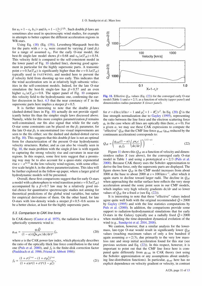
Fig. 11. Effective Qeff values (Eq. (22)) for the converged early O-starmodel (Table 1) and α= 2/3, as a function of velocity (upper panel) anddimensionless radius parameter X (lower panel).

for σ= d ln 3/d ln r − 1 and µ2∗ = 1 − R2

∗/r2. In Eq. (20) Q is the

line strength normalization due to Gayley (1995), representingthe ratio between the line force and the electron scattering forcege in the case where all lines are optically thin (here, α= 0). Fora given α, we may use these CAK expressions to compute the“effective” Qeff that the CMF line force gcmf (grad reduced by thecontinuum acceleration) corresponds to:

Qeff =

(gcmf(1 − α)

ge fd

(ρκecd3/dr

)α)1/(1−α)

. (22)

Figure 11 shows this Qeff as a function of velocity and dimen-sionless radius X (see above), for the converged early O-starmodel in Table 1 and using a prototypical α= 2/3 (Puls et al.2000). Because CAK theory uses the Sobolev approximation toderive the line force, only the supersonic parts are displayed. Thefigure shows how Qeff in the CMF model increases from about1000 at the base to about 2000 at 3≈ 100 km s−1, after which itagain starts to decline toward larger radii. The decline in Qeff

when approaching the stellar surface here reflects the very steepacceleration around the sonic point seen in our CMF models,which implies very high velocity gradients d3/dr and so lowervalues of Qeff for a fixed α (see Eq. (22)).

It is interesting to note that these “effective” values indeedagree quite well both with the original recommended Q≈ 2000by Gayley (1995) and with the line statistics computations byPuls et al. (2000). In addition, the comparisons provide somesupport to radiation-hydrodynamical simulations that for earlyO-stars in the Galaxy typically use a radially fixed Q = 2000when modeling the time-dependent dynamical evolution of thewind (e.g., Sundqvist et al. 2014, 2018).

We caution, however, that a similar analysis for the lower-mass, late-type O-star would result in significantly lower Qeff

values (reaching maximum values of only a few hundred ifagain assuming α= 2/3), due primarily to the very low mass-loss rate and steep initial acceleration found for this star (seeprevious sections and Eq. (22)). In this respect, however, it isimportant to point out that the CMF line force here is com-puted quite differently from gCAK in CAK theory (not usingthe Sobolev approximation or any assumptions about underly-ing line-distribution functions). In particular, gcmf here has noexplicit dependence on velocity gradient or velocity, in contrast

A126, page 11 of 13

A&A 632, A126 (2019)

to gCAK (Eq. (20)). As discussed below, this can have importantconsequences not only for direct comparisons of models, but alsofor the very nature of the steady wind solution.

5.4. Stability, uniqueness, and wind topology

The two base models presented above show a quite stable itera-tion behavior toward convergence. However, in our calculationswe find that this is not always the case. For some models, theiteration rather first proceeds as expected, toward lower andlower f max

err and toward a more and more constant M, but thennever reaches the (admittedly rather strict) convergence cri-teria discussed above. Instead, the model may experience analmost semi-cyclic behavior, wherein low values of f max

err can beobserved during semi-regular iteration intervals, but where theseminima never reach our selected criterion for convergence. Tothis end, it is neither clear what exactly causes this behavior, norif it is a numerical or physical effect (see further below).

For such simulations, for example the ones with the lower-most turbulent velocities displayed in Fig. 7, we then insteaduse the iteration with the lowest f max

err when selecting our finalmodel. We note that while these simulations are not formallyconverged, the range in the most important targeted parameter Mwith acceptably low f max

err is typically quite modest. Specificallyfor the case mentioned above, the lowest f max

err was on the orderof a few percent, making it above our convergence criterion herebut below that used by Sander et al. (2017) (5%) for example; thecorresponding mass-loss rates with f max

err < 10% lay in the range≈ (1.5−2.0)× 10−6 M� yr−1.

Indeed, since the steady-state e.o.m. Eq. (2) is nonlinear, it isnot a priori certain that a unique and stable solution can be found.For time-dependent wind models computed using distributionfunctions and the observer’s frame line force, this has been ana-lyzed by Poe et al. (1990) and Sundqvist & Owocki (2015). Fortheir parametrized line forces, these authors carried out topol-ogy analyses of the solution behavior at the critical sonic point4.It turns out that depending for example on the behavior of thesource function at the sonic point (Sundqvist & Owocki 2015),the wind topology can transition from a stable X-type with aunique solution to an unstable nodal type exhibiting degener-ate solutions. When such a wind model lies on the shallow partof this nodal topology branch, Poe et al. (1990) showed that aniteration scheme like that applied here on the time-independente.o.m. will not converge.

In this respect, it is important to point out that since the mod-els here compute grad as an explicit function only of radius (thusnot including any explicit velocity dependence), we are effec-tively forcing the solution to lie on the stable X-type branch,irrespective of what the “true” underlying solution actually is.Indeed, such forcing toward the X-type branch is effectively donealso in the alternative models by Sander et al. (2017) and Lucy(2007), where the former authors use a line acceleration depend-ing only on radius (like here) and the latter use one that dependsonly on velocity (thus neglecting the radial dependence).

In any case, a further topology analysis of numerical CMFmodels such as those presented here would require a com-pletely new parametrization of the line force in order to properlyexamine the solution behavior for different stellar ranges. Thislies beyond the scope of the present paper but should be afocus for follow-up work targeting detailed comparisons of our

4 Since the velocity gradient does not appear explicitly in suchobserver’s frame calculations of grad, the sonic point remains the onlycritical point in the steady limit.

new steady-state models with time-dependent hydrodynamiccalculations.

5.5. The “weak-wind” problem

The low mass-loss rate derived for the late O-star in Sect. 4.5is generally consistent with the empirical finding that obser-vationally inferred mass-loss rates of late O-dwarfs typicallyare much lower than suggested by previous theoretical models(the so-called “weak-wind” problem, see, e.g., Puls et al. 2008;Marcolino et al. 2009). Indeed, for our late-O model star weobtain a rate that is approximately nine times lower than that pre-dicted by the theoretical mass-loss recipe by Vink et al. (2000),as already discussed in Sect. 5.1.

On the other hand, the accompanying very high terminalwind speeds we derive have not been observed. This suggeststhat some additional physics may act to reduce the radiationforce in the outer parts of these low-density winds from GalacticO-dwarfs (or at least make them invisible to UV observations).In this respect, one speculation is that LDI-generated shocks(see Sect. 4.3) might not be able to efficiently cool in such low-density environments, meaning that also the bulk wind is leftmuch hotter than expected. Such a shock-heated bulk wind seemsto be suggested by the X-ray observations of low-density windsby Huenemoerder et al. (2012) and Doyle et al. (2017), who alsosuggested that the “weak-wind” problem might simply be relatedto insufficient cooling (see also Lucy 2012). Indeed, from softX-ray ROSAT observations already Drew et al. (1994) suggestedthat large portions of hot, uncooled gas might exist in the outerregions of low-density winds. If true, such extended hot regionscould then also imply a significantly reduced radiative driving inthese wind parts.

We note that this scenario is quite different from that exam-ined in Sect. 4.3 for the early O-star wind with a higher density.Specifically, although the included X-rays there may have asignificant impact on the ionization balance of some specificelements, the temperature structure of the bulk wind is basi-cally unaffected. The possibility of a hot bulk wind shouldbe further examined in future work, preferably by performingLDI simulations tailored to low-density winds and including aproper treatment of the shock-heated gas and associated coolingprocesses.

6. Summary and future work

We have developed new radiation-driven wind models for hot,massive stars, suitable for basic predictions of global parameterslike mass-loss and wind-momentum rates. The simulations arebased on an iterative grid solution to the spherically symmet-ric, steady-state e.o.m., using full NLTE CMF radiative transfersolutions for calculation of the radiative acceleration responsiblefor the wind driving.

In this first paper, we present models representing two proto-typical O-stars in the Galaxy, one “early” with a higher massM∗/M� ≈ 59 and one “late” with a lower mass M∗/M� ≈ 27.Table 1 summarizes the results, with predicted mass-loss ratesM = 1.51 × 10−6 M� yr−1 and M = 2.55 × 10−8 M� yr−1 for thetwo models, respectively. In Sect. 4, we further discussed insome detail the influence on the model predictions from addi-tional parameters like wind clumping, turbulent speeds, andchoice of temperature structure calculation.

Overall, our results seem to agree rather well with othersteady-state wind models that do not rely on the Sobolevapproximation for computation of the radiative line acceleration

A126, page 12 of 13

J. O. Sundqvist et al.: Mass loss

(Lucy 2010; Krticka & Kubát 2017; Sander et al. 2017). A keyresult is that the mass-loss rates we predict are significantly lowerthan those (Vink et al. 2000, 2001) normally included in modelsof massive-star evolution. Two likely reasons for the lower valuesare the use of CMF transfer versus the Sobolev approximationand also the somewhat different nature of the NLTE solutiontechniques used here and by Vink et al. Our results thus add tosome previous notions (e.g., Sundqvist et al. 2011; Najarro et al.2011; Šurlan et al. 2013; Cohen et al. 2014; Krticka & Kubát2017; Keszthelyi et al. 2017) that O-star mass-loss rates may beoverestimated in current massive-star evolution models and that(considering the big impact of mass loss on the lives of massivestars) new rates might be needed.

In this planned paper series, we intend to work toward pro-viding such updated radiation-driven mass loss for direct use instellar evolution calculations (Björklund et al., in prep.). Otherfollow-ups include investigations of the mass-loss vs. metallicitydependence in our models, comparison to time-dependent simu-lations, and extension of the current O-star models to B-stars (inparticular supergiants across the bistability jump) and potentiallyalso Wolf-Rayet stars.

Acknowledgements. We thank the referee for useful comments on the manuscript.We also thank Stan Owocki for so many fruitful discussions on line-driving.J.O.S. and R.B. also thank the KU Leuven EQUATION-group for their valu-able inputs as well as their weekly supply of fika, and also acknowledgethe Belgian Research Foundation Flanders (FWO) Odysseus program undergrant number G0H9218N. J.O.S. further acknowledges previous support fromthe European Union Horizon 2020 research and innovation program underthe Marie-Sklodowska-Curie grant agreement No 656725. F.N. acknowledgesfinancial support through Spanish grants ESP2015-65597-C4-1-R and ESP2017-86582 C4-1-R (MINECO/FEDER).

References

Anders, E., & Grevesse, N. 1989, Geochim. Cosmochim. Acta, 53, 197Asplund, M., Grevesse, N., Sauval, A. J., & Scott, P. 2009, ARA&A, 47, 481Bouret, J.-C., Lanz, T., & Hillier, D. J. 2005, A&A, 438, 301Carneiro, L. P., Puls, J., Sundqvist, J. O., & Hoffmann, T. L. 2016, A&A, 590,

A88Castor, J. I., Abbott, D. C., & Klein, R. I. 1975, ApJ, 195, 157Cohen, D. H., Wollman, E. E., Leutenegger, M. A., et al. 2014, MNRAS, 439,

908Doyle, T. F., Petit, V., Cohen, D., & Leutenegger, M. 2017, in The Lives and

Death-Throes of Massive Stars, eds. J. J. Eldridge, J. C. Bray, L. A. S.McClelland, & L. Xiao, IAU Symp., 329, 395

Drew, J. E., Hoare, M. G., & Denby, M. 1994, MNRAS, 266, 917Feldmeier, A., Puls, J., & Pauldrach, A. W. A. 1997, A&A, 322, 878Friend, D. B., & Abbott, D. C. 1986, ApJ, 311, 701Fullerton, A. W., Massa, D. L., & Prinja, R. K. 2006, ApJ, 637, 1025

Gayley, K. G. 1995, ApJ, 454, 410Gräfener, G., & Hamann, W.-R. 2005, A&A, 432, 633Hillier, D. J., & Miller, D. L. 1998, ApJ, 496, 407Hubeny, I., & Mihalas, D. 2014, Theory of Stellar Atmospheres (Princeton:

Princeton University Press)Huenemoerder, D. P., Oskinova, L. M., Ignace, R., et al. 2012, ApJ, 756, L34Keszthelyi, Z., Puls, J., & Wade, G. A. 2017, A&A, 598, A4Krticka, J., & Kubát, J. 2007, A&A, 464, L17Krticka, J., & Kubát, J. 2010, A&A, 519, A50Krticka, J., & Kubát, J. 2017, A&A, 606, A31Kudritzki, R. P., Pauldrach, A., & Puls, J. 1987, A&A, 173, 293Langer, N. 2012, ARA&A, 50, 107Lucy, L. B. 1971, ApJ, 163, 95Lucy, L. B. 2007, A&A, 468, 649Lucy, L. B. 2010, A&A, 512, A33Lucy, L. B. 2012, A&A, 544, A120Lucy, L. B., & Solomon, P. M. 1970, ApJ, 159, 879Marcolino, W. L. F., Bouret, J., Martins, F., et al. 2009, A&A, 498, 837Martins, F., Schaerer, D., Hillier, D. J., et al. 2005, A&A, 441, 735Massa, D., Fullerton, A. W., & Prinja, R. K. 2017, MNRAS, 470, 3765Meynet, G., Maeder, A., Schaller, G., Schaerer, D., & Charbonnel, C. 1994,

A&AS, 103, 97Mihalas, D. 1978, Stellar Atmospheres, 2nd edn. (San Francisco, W. H. Freeman

and Co.), 650Mokiem, M. R., de Koter, A., Vink, J. S., et al. 2007, A&A, 473, 603Muijres, L. E., de Koter, A., Vink, J. S., et al. 2011, A&A, 526, A32Najarro, F., Hanson, M. M., & Puls, J. 2011, A&A, 535, A32Owocki, S. P., & Puls, J. 1999, ApJ, 510, 355Owocki, S. P., & Rybicki, G. B. 1984, ApJ, 284, 337Owocki, S. P., Castor, J. I., & Rybicki, G. B. 1988, ApJ, 335, 914Pauldrach, A. W. A., & Puls, J. 1990, A&A, 237, 409Pauldrach, A., Puls, J., & Kudritzki, R. P. 1986, A&A, 164, 86Pauldrach, A. W. A., Hoffmann, T. L., & Lennon, M. 2001, A&A, 375, 161Poe, C. H., Owocki, S. P., & Castor, J. I. 1990, ApJ, 358, 199Puls, J. 2017, in The Lives and Death-Throes of Massive Stars, eds. J. J. Eldridge,

J. C. Bray, L. A. S. McClelland, & L. Xiao, IAU Symp., 329, 435Puls, J., Springmann, U., & Lennon, M. 2000, A&AS, 141, 23Puls, J., Urbaneja, M. A., Venero, R., et al. 2005, A&A, 435, 669Puls, J., Markova, N., Scuderi, S., et al. 2006, A&A, 454, 625Puls, J., Vink, J. S., & Najarro, F. 2008, A&ARv, 16, 209Ramírez-Agudelo, O. H., Sana, H., de Koter, A., et al. 2017, A&A, 600, A81Sander, A. A. C., Hamann, W.-R., Todt, H., Hainich, R., & Shenar, T. 2017,

A&A, 603, A86Santolaya-Rey, A. E., Puls, J., & Herrero, A. 1997, A&A, 323, 488Shenar, T., Oskinova, L., Hamann, W. R., et al. 2015, ApJ, 809, 135Smith, N. 2014, ARA&A, 52, 487Sundqvist, J. O., & Owocki, S. P. 2013, MNRAS, 428, 1837Sundqvist, J. O., & Owocki, S. P. 2015, MNRAS, 453, 3428Sundqvist, J. O., & Puls, J. 2018, A&A, 619, A59Sundqvist, J. O., Puls, J., Feldmeier, A., & Owocki, S. P. 2011, A&A, 528, 64Sundqvist, J. O., Puls, J., & Owocki, S. P. 2014, A&A, 568, A59Sundqvist, J. O., Owocki, S. P., & Puls, J. 2018, A&A, 611, A17Šurlan, B., Hamann, W.-R., Aret, A., et al. 2013, A&A, 559, A130Vink, J. S., de Koter, A., & Lamers, H. J. G. L. M. 2000, A&A, 362, 295Vink, J. S., de Koter, A., & Lamers, H. J. G. L. M. 2001, A&A, 369, 574

A126, page 13 of 13