New Options to Visualize Systems of Differential Equations in

Maple ∗

Mohammad ali Ebrahimi and Michael Monagan

Department of Mathematics, Simon Fraser Universitymebrahim@cecm.sfu.ca and mmonagan@cecm.sfu.ca

Abstract

The DEplot command in Maple is used to show the direction field and solution curves of adifferential equation or system of differential equations. We present new options created for theDEplot command for enhancing the visualization of a direction field and for animating a directionfield and the solution curves in time. We present a new Maplet, DEplotlet(DEplotInteractive),which simplifies the use of the DEplot command. We have also designed a database of differentsystems of differential equations which can be easily modified by the instructor. The databaseincludes the Lotka-Volterra predator-prey system and the Kermack-McKendric epidemic model.It includes default choices for the parameters and for initial values so that the instructor andstudent can obtain a good plot with a single mouse click.

1 Introduction:

Consider the autonomous system x′(t) = f(x, y), y′(t) = g(x, y) where x, y ∈ R. One can drawsmall line segments with a slope g(xi,yi)

f(xi,yi)at any desired point (xi, yi). Each line segment is then

tangent to the solution at the point (xi, yi). The set of all these line segments is called the directionfield. By plotting the direction field of the system one can get a good approximation of the solutionand its properties. In addition plotting direction fields is fast and easy, since there is no need tosolve ordinary differential equation(’s). Direction fields can also be used for testing the accuracy ofthe numerical solutions. For example, the Lotka-Volterra system

x′(t) = α x(t)− b x(t)y(t), y′(t) = −β y(t) + c x(t)y(t) (1)

is a predator-prey model. Here, x(t) is the population of the prey at time t, y(t) is the populationof the predator at time t, α > 0 is the birth rate of the prey, β > 0 is the death rate of the predatorand the terms c x(t)y(t) and −d x(t)y(t) where c > 0 and d > 0 describe the interaction of thepredator and prey. Throughout the paper we use the following system for showing plots.

des := [x′(t) = x(t)(1− y(t)), y′(t) = .3y(t)(−1 + x(t))].

Figure 1 shows a plot of the system obtained using Maple’s DEplot command. Notice that insteadof drawing line segments, Maple shows little arrows to indicate the direction of the solution at themidpoint of the arrow.

∗Supported by NSERC of Canada and the MITACS os Canada.

1

2

1.5 2

y

0

1.5

0.5

1

0.5 10

x

Figure 1: This is a direction field for the Lotka-Volterra model created by the Maple com-mand DEplot. The Maple command used is: DEplot(des, [x(t),y(t)], t=1..10, x=0..2, y=0..2,

arrows=large);

In this paper we show new options and tools created to enhance the visuals of the directionfields for the system of differential equations. In section 2 we discuss options to show the velocityof the solutions, in section 3 we give options to improve the visualization of the direction field, insection 4 we give two new arrow styles to improve the approximation of the direction field, and insection 5 options for animating the direction field and solution curves. In section 6 we describe theDEplotInteractive Maplet and the database of systems of differential equations.

2 Velocity Options

In Figure 1, we can see the “direction” but not the velocity of the direction field. The velocityoption determines the norm of the speed of the solution at each point. For example if we havethe system {y′(t) = f(x, y), x′(t) = g(x, y)} then the norm of the speed at the point (x, y) can berepresented by

√f(x, y)2 + g(x, y)2. We have used this information and created two options for

showing the norm of the speed of the solution of a system of differential equation at different pointsin the DEplot command. Our first solution to present the velocity is by color. The second solutionis by the size of the arrows. In order to create a direction field which can demonstrate the norm ofthe speed at the position of each arrow, first we need to find the largest value of the speed amongall the values of speed of the arrows. This is so we can scale the velocities, so they are between zeroto 1. After finding the largest value of the velocities then at each point, where the arrow is located,

the final value of velocity is represented by the value of√

f(x,y)2+g(x,y)2

MAX(√

f(x,y)2+g(x,y)2).

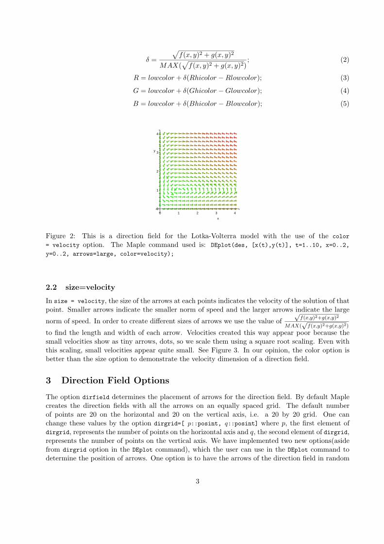
2.1 color=velocity[hicolor, lowcolor]

In this option the color of the arrows is determined by the velocity of the field. The low and highvelocity colors are specified as the index of velocity. The option color = velocity can be used withthe default of [green, red]. To find the RGB color value of each grid point, we use the followingformula:

2

δ =

√f(x, y)2 + g(x, y)2

MAX(√

f(x, y)2 + g(x, y)2); (2)

R = lowcolor + δ(Rhicolor −Rlowcolor); (3)

G = lowcolor + δ(Ghicolor −Glowcolor); (4)

B = lowcolor + δ(Bhicolor −Blowcolor); (5)

4

3 4

y

0

3

1

2

1 20

x

Figure 2: This is a direction field for the Lotka-Volterra model with the use of the color

= velocity option. The Maple command used is: DEplot(des, [x(t),y(t)], t=1..10, x=0..2,

y=0..2, arrows=large, color=velocity);

2.2 size=velocity

In size = velocity, the size of the arrows at each points indicates the velocity of the solution of thatpoint. Smaller arrows indicate the smaller norm of speed and the larger arrows indicate the large

norm of speed. In order to create different sizes of arrows we use the value of√

f(x,y)2+g(x,y)2

MAX(√

f(x,y)2+g(x,y)2)

to find the length and width of each arrow. Velocities created this way appear poor because thesmall velocities show as tiny arrows, dots, so we scale them using a square root scaling. Even withthis scaling, small velocities appear quite small. See Figure 3. In our opinion, the color option isbetter than the size option to demonstrate the velocity dimension of a direction field.

3 Direction Field Options

The option dirfield determines the placement of arrows for the direction field. By default Maplecreates the direction fields with all the arrows on an equally spaced grid. The default numberof points are 20 on the horizontal and 20 on the vertical axis, i.e. a 20 by 20 grid. One canchange these values by the option dirgrid=[ p::posint, q::posint] where p, the first element ofdirgrid, represents the number of points on the horizontal axis and q, the second element of dirgrid,represents the number of points on the vertical axis. We have implemented two new options(asidefrom dirgrid option in the DEplot command), which the user can use in the DEplot command todetermine the position of arrows. One option is to have the arrows of the direction field in random

3

4

3 4

y

0

3

1

2

1 20

x

Figure 3: This is a direction field for the Lotka-Volterra model with the use of the size = velocity

command. The Maple command used is: DEplot(des, [x(t),y(t)], t=1..10, x=0..2, y=0..2,

arrows=large, size=velocity);

positions. The second option is that the user can determine the position of the arrows by a list ofpoints.

3.1 dirfield=positive integer:

To enhance the visualization of the direction field one can use the new command dirfield =

n::posint to create a direction field with n randomly positioned arrows. See Figure 4. In ouropinion, random position direction field gives the best visual.

y

x

2

2

1.5

1

1.5

0.5

010.50

y

x

2

2

1.5

1

1.5

0.5

010.50

Figure 4: Direction field for the Lotka-Volterra model with the use of the dirfield = 400 command.The Maple command used is: DEplot(des, [x(t),y(t)], t=1..10, x=0..2, y=0..2, arrows=large,

dirfield=400); The second plot is the plot of the same system but in a rectangular grid. Incomparison of the two plots we see that the random positioned field gives a better visual.

3.2 dirfield = [points]

In addition to the dirfield = n::posint option, we have implemented the the option dirfield =

[points]. With this option one can assign the desired positions of the arrows manually. See Figure

4

5.

x

y

2.5

2.5

2

1.5

2

1

0.5

1.50

-0.5

10.50-0.5

Figure 5: Direction field for the Lotka-Volterra model with the use of the dirfield =

[points] command. The command used is: DEplot(des, [x(t),y(t)], t=1..10, x=0..2, y=0..2,

arrows=large, dirfield=[[1.1,1.3],[1.5,1.4],[0.21,1.01],[0.01,0.01],[1,0.5],[0.5,2]]);

4 New Arrows:

To improve the visualization for the direction field, further, we have created new objects (fish shape)for which the curvature of each fish approximates the solution curve. The curvature of each fishis approximated by the modified Euler’s method. These objects help the user to have a betterapproximation of the solution to the system of differential equations. See Figure 6.

y

x

2

2

1.5

1

1.5

0.5

010.50 2

x

1.5

1

y

1.5

2

0.5

10.50

0

Figure 6: This is a direction field for the Lotka-Volterra model with the use of the arrow = fish com-mand. The command used is: DEplot(des, [x(t),y(t)], t=1..10, x=0..2, y=0..2, arrows=fish,

dirfield=500); In comparison of the two plots we see that the plot with fishes gives a sharperapproximation of the solution.

5

4.1 Method:

Lets assume we want to create a fish at the point (a, b) for autonomous system {y′(t) = f(x, y), x′(t) =g(x, y)}. Evaluating the two functions f(x, y) and g(x, y) at the point (a, b) we set µ = f(a,b)

g(a,b) ,(a′, b′) = (a, b) + µ(dx, dy), and (a′′, b′′) = (a, b) + −µ(dx, dy) where dx and dy are small. Thetwo points (a′, b′) and (a′′, b′′) are approximations of two points of the solution curve which passesthrough the point (a, b). One way to improve this approximation is to use the Euler’s improvedmethod. Hence, we do another function evaluation at (a′, b′) and at (a′′, b′′) and find ω = f(a′,b′)

g(a′,b′)

and ν = f(a′′,b′′)g(a′′,b′′) which leads us to find (a1, b1) = (a, b) + (−µ+ω

2 )(dx, dy) and (a2, b2) = (a, b) +

(µ+ν2 )(dx, dy). see Figure 7.

Figure 7: Steps to find the two end points (a1, b1), and(a2, b2) of the fish via modified Euler’smethod. ξ1 = µ+ν

2 , ξ2 = −µ+ω2 .

We now have three points (a, b), (a1, b1), and (a2, b2). To approximate the solution of f(x, y), g(x, y)near x = a, y = b, we can find a quadratic curve which fits these three points. Hence, we have aparametric quadratic approximation with respect to t ∈ [0, 2] of the solution curve passing throughthe point (a, b) where x(0) = a and y(0) = b.

Figure 8: Parametric quadratic polynomial fit on the three points

The parametric solution to the quadratic curve which passes through the three points (a, b), (a1, b1),and (a2, b2) is given by:

6

x(t) = ((a2

2− a +

a1

2)t− 3a2

2+ 2a− a1

2)t + a2 (6)

y(t) = ((b2

2− b +

b1

2)t− 3b2

2+ 2b− b1

2)t + b2 (7)

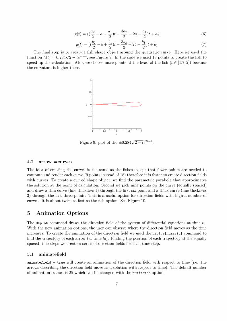
The final step is to create a fish shape object around the quadratic curve. Here we used thefunction h(t) = 0.284

√2− te2t−4, see Figure 9. In the code we used 18 points to create the fish to

speed up the calculation. Also, we choose more points at the head of the fish (t ∈ [1.7, 2]) becausethe curvature is higher there.

y

t

1

2

0.5

0

1.5

-0.5

-110.50

Figure 9: plot of the ±0.284√

2− te2t−4.

4.2 arrows=curves

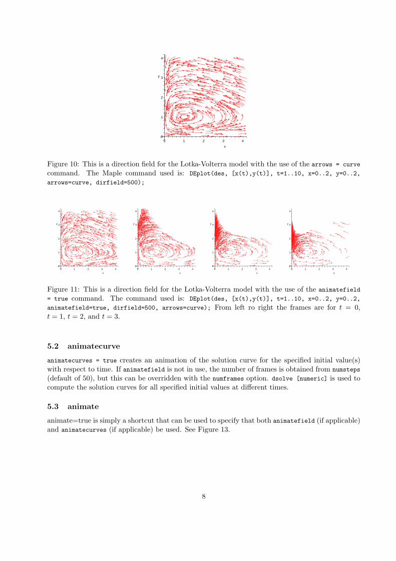
The idea of creating the curves is the same as the fishes except that fewer points are needed tocompute and render each curve (9 points instead of 18) therefore it is faster to create direction fieldswith curves. To create a curved shape object, we find the parametric parabola that approximatesthe solution at the point of calculation. Second we pick nine points on the curve (equally spaced)and draw a thin curve (line thickness 1) through the first six point and a thick curve (line thickness3) through the last three points. This is a useful option for direction fields with high a number ofcurves. It is about twice as fast as the fish option. See Figure 10.

5 Animation Options

The DEplot command draws the direction field of the system of differential equations at time t0.With the new animation options, the user can observe where the direction field moves as the timeincreases. To create the animation of the direction field we used the dsolve[numeric] command tofind the trajectory of each arrow (at time t0). Finding the position of each trajectory at the equallyspaced time steps we create a series of direction fields for each time step.

5.1 animatefield

animatefield = true will create an animation of the direction field with respect to time (i.e. thearrows describing the direction field move as a solution with respect to time). The default numberof animation frames is 25 which can be changed with the numframes option.

7

y

x

4

4

3

2

3

1

0210

Figure 10: This is a direction field for the Lotka-Volterra model with the use of the arrows = curve

command. The Maple command used is: DEplot(des, [x(t),y(t)], t=1..10, x=0..2, y=0..2,

arrows=curve, dirfield=500);

y

x

4

4

3

2

3

1

0210

y

x

4

4

3

2

3

1

0210

y

x

4

4

3

2

3

1

0210

y

x

4

4

3

2

3

1

0210

Figure 11: This is a direction field for the Lotka-Volterra model with the use of the animatefield

= true command. The command used is: DEplot(des, [x(t),y(t)], t=1..10, x=0..2, y=0..2,

animatefield=true, dirfield=500, arrows=curve); From left ro right the frames are for t = 0,t = 1, t = 2, and t = 3.

5.2 animatecurve

animatecurves = true creates an animation of the solution curve for the specified initial value(s)with respect to time. If animatefield is not in use, the number of frames is obtained from numsteps

(default of 50), but this can be overridden with the numframes option. dsolve [numeric] is used tocompute the solution curves for all specified initial values at different times.

5.3 animate

animate=true is simply a shortcut that can be used to specify that both animatefield (if applicable)and animatecurves (if applicable) be used. See Figure 13.

8

x

32.521.51

y

0.5

2

1.5

0

1

0.5

0

x

32.521.51

y

0.5

2

1.5

0

1

0.5

0

x

32.521.51

y

0.5

2

1.5

0

1

0.5

0

x

32.521.51

y

0.5

2

1.5

0

1

0.5

0

Figure 12: This is a direction field for the Lotka-Volterra model with one solution curve which isanimated in time. The Maple command used is: DEplot(des, [x(t),y(t)], t=1..10, x=0.1..3,

y=0..2, animatecurve=true, dirfield=200, [[x(0)=0.5, y(0)=0.5]], arrows=fish); From left toright the frames are for t = 0, t = 2, t = 4, and t = 6.

x

32.521.51

y

0.5

2

1.5

0

1

0.5

0

x

32.521.51

y

0.5

2

1.5

0

1

0.5

0

x

32.521.51

y

0.5

2

1.5

0

1

0.5

0

x

32.521.51

y

0.5

2

1.5

0

1

0.5

0

Figure 13: This is a direction field for the Lotka-Volterra model with the use of the animate

= true option. The Maple command used is: DEplot(des, [x(t),y(t)], t=1..10, x=0.1..3,

y=0..2, animate=true, dirfield=200, [[x(0)=0.5, y(0)=0.5]], arrows=fish); From left to rightthe frames are for t = 0, t = 2, t = 4, and t = 6.

6 DEplot Interactive, GUI

In addition to the new options for the DEplot command we have created a Maplet, DEplotInteractive,which can read and write systems of differential equations from and into a text editable library(database) and produce the direction field for the chosen system. Aside from plotting, the user canchange the values of parameters, and initial values in the system, as well as some of the options inDEplot command. For example, the arrows, range of variables, arrow types, initial values option,and dirfield option. The editable database is designed so that it is valid Maple input, thus it is aplain text file, so that the user can read and edit the database easily. The format for the input isdescribed in figure 14 below. Because it is valid Maple input, the Maple user will not need to learnanything as the input format is obvious from the examples in the database. The idea of creatingthe database is to help educators browse different behaviors of a system of differential equationswith different parameter settings and different initial values instantly. This will lead to the idea ofhaving Maple databases of systems, functions and perhaps plots for other commands other thanDEplot for educators. The database is an alternative way of storing examples than the examplesin the Maple’s help pages. We think that such databases for other Maple commands and packagesshould be developed in the future.

9

Figure 14: This is a sample of the editable database file. The first line of each system indicates thename of the system. The second line specifies the system. The third line is the list of all parametersused in the system and their default values. The fourth line is the list of initial values to be used,and the fifth line is the names of the variables and their default ranges.

Figure 15: Left figure: This is the maplet for adding the system with parameters to the database.The name of the system as well as other information about the system can be specified. Rightfigure: This is the main maplet which user can choose one of the systems, read from the database,to DEplot (or animate). In addition, the user can choose to add a new system to the library.

10

Figure 16: Above is a sample of the DEplotlet page. The top window shows the name of the systemand the system in a Math-ML view. The two windows below the Math-ML view are for differentoptions of DEplot and also values of the parameters and the initial values. These may be changedby the user. Clicking on the refresh button replots the system

7 Acknowledgment

We thank Allan Wittkopf for installing the program, helping with the test file, and his helpfulcomments. We also thank Robert Corless for his helpful comments.

References

[1] William E.Boyce, Richard C. Diprima. Elementary Differential Equation and Boundary Valueproblems.

[2] Stan Wagon, Dan Schwalbe. VisualDsolve. Mathematica Electronic Journal.

[3] M. Monagan, K. Geddes, G. Labahn, S. Vorkoetter, J. McCarra, and P. deMarco. Maple 9Advanced programming Guide. Maplesoft, 2003.

11