new methods for surface reconstruction from range images · 2000-08-30 · new methods for surface...
TRANSCRIPT

NEW METHODS FOR SURFACE RECONSTRUCTION
FROM RANGE IMAGES
A DISSERTATION
SUBMITTED TO THE DEPARTMENT OF ELECTRICAL ENGINEERING
AND THE COMMITTEE ON GRADUATE STUDIES
OF STANFORD UNIVERSITY
IN PARTIAL FULFILLMENT OF THE REQUIREMENTS
FOR THE DEGREE OF
DOCTOR OF PHILOSOPHY
Brian Lee Curless
June, 1997

c Copyright 1997 by Brian Lee Curless
All Rights Reserved
ii

I certify that I have read this dissertation and that in my opinion it is fully adequate,
in scope and in quality, as a dissertation for the degree of Doctor of Philosophy.
Marc Levoy (Principal Adviser)
I certify that I have read this dissertation and that in my opinion it is fully adequate,
in scope and in quality, as a dissertation for the degree of Doctor of Philosophy.
Pat Hanrahan
I certify that I have read this dissertation and that in my opinion it is fully adequate,
in scope and in quality, as a dissertation for the degree of Doctor of Philosophy.
David Heeger
Approved for the University Committee on Graduate Studies:
iii

iv

To Jelena
v

vi

Abstract
The digitization and reconstruction of 3D shapes has numerous applications in areas that
include manufacturing, virtual simulation, science, medicine, and consumer marketing. In
this thesis, we address the problem of acquiring accurate range data through optical trian-
gulation, and we present a method for reconstructing surfaces from sets of data known as
range images.
The standard methods for extracting range data from optical triangulation scanners are
accurate only for planar objects of uniform reflectance. Using these methods, curved sur-
faces, discontinuous surfaces, and surfaces of varying reflectance cause systematic distor-
tions of the range data. We present a new ranging method based on analysis of the time
evolution of the structured light reflections. Using this spacetime analysis, we can correct
for each of these artifacts, thereby attaining significantly higher accuracy using existing
technology. When using coherent illumination such as lasers, however, we show that laser
speckle places a fundamental limit on accuracy for both traditional and spacetime triangu-
lation.
The range data acquired by 3D digitizers such as optical triangulation scanners com-
monly consists of depths sampled on a regular grid, a sample set known as a range image. A
number of techniques have been developed for reconstructing surfaces by integrating groups
of aligned range images. A desirable set of properties for such algorithms includes: incre-
mental updating, representation of directional uncertainty, the ability to fill gaps in the re-
construction, and robustness in the presence of outliers and distortions. Prior algorithms
possess subsets of these properties. In this thesis, we present an efficient volumetric method
for merging range images that possesses all of these properties. Using this method, we are
able to merge a large number of range images (as many as 70) yielding seamless, high-detail
models of up to 2.6 million triangles.
vii

viii

Acknowledgments
I would like to thank the many people who contributed in one way or another to this the-
sis. I owe a great debt to my adviser, Marc Levoy, who inspired me to enter the exciting
arena of computer graphics. The road to a Ph.D. is usually a bumpy one, and mine was no
exception. In the end, Marc’s unerring intuitions and infectious enthusiasm sent me down
a very rewarding path. I would also thank the members of my reading committee, Pat Han-
rahan and David Heeger, for their interest in this work. Early discussions with Pat while
developing the ideas about space carving in Chapter 6 were especially helpful.
Next, I would like to thank my colleagues in the Stanford Computer Graphics Labora-
tory. As members of the 3D Fax Project, Greg Turk, Venkat Krishnamurthy, and Brian Frey-
burger have been particularly supportive. Brian developed the ideas for space carving with
triangulation scanners (Section 6.4). In addition, discussions with Phil Lacroute were cru-
cial to making the volumetric algorithm efficient (Section 7.2). Homan Igehy wrote the fast
rasterizer used for range image resampling (Section 7.2), and Matt Pharr wrote the accessi-
bility shader used to create the rendering in Figure 8.6b. Bill Lorensen provided marching
cubes tables and mesh decimation software and managed the production of the 3D hardcopy.
Special thanks go to Charlie Orgish and John Gerth for maintaining sanity among the
machines (and therefore the students) in the graphics laboratory. Sarah Bezier and Ada
Glucksman cheerfully shielded me from the inner-workings of University bureaucracy.
Cyberware Laboratories provided the scanner used to collect data in this thesis. I am
particularly grateful to David Addleman and George Dabrowski at Cyberware for their as-
sistance and encouragement. Funding for this work came from the National Science Foun-
dation under contract CCR-9157767 and from Interval Research Corporation.
I would like to thank my parents, Richard and Diane, my brother, Chris, and my sisters,
ix

Ann and Laura. With their support, I knew I would persevere through the years. Finally,
my deepest gratitude goes to my wife, Jelena. She calmed me in moments of panic and had
faith in me during times of doubt. I dedicate this thesis to her.
x

Contents
v
Abstract vii
Acknowledgments ix
1 Introduction 1
1.1 Applications . . . . . . . . . . . . . . . . . . . . . . . . . . . . . . . . . . 2
1.1.1 Reverse engineering . . . . . . . . . . . . . . . . . . . . . . . . . 2
1.1.2 Collaborative design . . . . . . . . . . . . . . . . . . . . . . . . . 2
1.1.3 Inspection . . . . . . . . . . . . . . . . . . . . . . . . . . . . . . . 3
1.1.4 Special effects, games, and virtual worlds . . . . . . . . . . . . . . 3
1.1.5 Dissemination of museum artifacts . . . . . . . . . . . . . . . . . . 3
1.1.6 Medicine . . . . . . . . . . . . . . . . . . . . . . . . . . . . . . . 3
1.1.7 Home shopping . . . . . . . . . . . . . . . . . . . . . . . . . . . . 4
1.2 Methods for 3D Digitization . . . . . . . . . . . . . . . . . . . . . . . . . 4
1.3 Surface reconstruction from range images . . . . . . . . . . . . . . . . . . 9
1.3.1 Range images . . . . . . . . . . . . . . . . . . . . . . . . . . . . . 9
1.3.2 Surface reconstruction . . . . . . . . . . . . . . . . . . . . . . . . 10
1.4 The 3D Fax Project . . . . . . . . . . . . . . . . . . . . . . . . . . . . . . 12
1.5 Contributions . . . . . . . . . . . . . . . . . . . . . . . . . . . . . . . . . 15
1.6 Organization . . . . . . . . . . . . . . . . . . . . . . . . . . . . . . . . . 16
2 Optical triangulation: limitations and prior work 18
2.1 Triangulation Configurations . . . . . . . . . . . . . . . . . . . . . . . . . 19
2.1.1 Structure of the illuminant . . . . . . . . . . . . . . . . . . . . . . 19
xi

2.1.2 Type of illuminant . . . . . . . . . . . . . . . . . . . . . . . . . . 20
2.1.3 Sensor . . . . . . . . . . . . . . . . . . . . . . . . . . . . . . . . . 21
2.1.4 Scanning method . . . . . . . . . . . . . . . . . . . . . . . . . . . 21
2.2 Limitations of traditional methods . . . . . . . . . . . . . . . . . . . . . . 21
2.2.1 Geometric intuition . . . . . . . . . . . . . . . . . . . . . . . . . . 22
2.2.2 Quantifying the error . . . . . . . . . . . . . . . . . . . . . . . . . 26
2.2.3 Focusing the beam . . . . . . . . . . . . . . . . . . . . . . . . . . 28
2.2.4 Influence of laser speckle . . . . . . . . . . . . . . . . . . . . . . 30
2.3 Prior work on triangulation error . . . . . . . . . . . . . . . . . . . . . . . 36
3 Spacetime Analysis 38
3.1 Geometric intuition . . . . . . . . . . . . . . . . . . . . . . . . . . . . . . 38
3.2 A complete derivation . . . . . . . . . . . . . . . . . . . . . . . . . . . . 40
3.3 Generalizing the geometry . . . . . . . . . . . . . . . . . . . . . . . . . . 44
3.4 Influence of laser speckle . . . . . . . . . . . . . . . . . . . . . . . . . . . 46
3.5 A Signal Processing Perspective . . . . . . . . . . . . . . . . . . . . . . . 51
3.5.1 Ideal triangulation impulse response . . . . . . . . . . . . . . . . . 51
3.5.2 Filtering, noise, sampling, and reconstruction . . . . . . . . . . . . 53
3.5.3 The spacetime spectrum . . . . . . . . . . . . . . . . . . . . . . . 54
3.5.4 Widening the laser sheet . . . . . . . . . . . . . . . . . . . . . . . 56
3.5.5 Improving resolution . . . . . . . . . . . . . . . . . . . . . . . . . 58
4 Spacetime analysis: implementation and results 60
4.1 Hardware . . . . . . . . . . . . . . . . . . . . . . . . . . . . . . . . . . . 60
4.2 The spacetime algorithm . . . . . . . . . . . . . . . . . . . . . . . . . . . 62
4.2.1 Fast rotation of the spacetime image . . . . . . . . . . . . . . . . . 65
4.2.2 Interpolating the spacetime volume . . . . . . . . . . . . . . . . . 69
4.3 Results . . . . . . . . . . . . . . . . . . . . . . . . . . . . . . . . . . . . 70
4.3.1 Reflectance correction . . . . . . . . . . . . . . . . . . . . . . . . 70
4.3.2 Shape correction . . . . . . . . . . . . . . . . . . . . . . . . . . . 71
4.3.3 Speckle . . . . . . . . . . . . . . . . . . . . . . . . . . . . . . . . 73
4.3.4 Complex objects . . . . . . . . . . . . . . . . . . . . . . . . . . . 73
xii

4.3.5 Remaining sources of error . . . . . . . . . . . . . . . . . . . . . . 77
5 Surface estimation from range images 78
5.1 Prior work in surface reconstruction from range data . . . . . . . . . . . . 79
5.1.1 Unorganized points: polygonal methods . . . . . . . . . . . . . . . 79
5.1.2 Unorganized points: implicit methods . . . . . . . . . . . . . . . . 79
5.1.3 Structured data: polygonal methods . . . . . . . . . . . . . . . . . 80
5.1.4 Structured data: implicit methods . . . . . . . . . . . . . . . . . . 80
5.1.5 Other related work . . . . . . . . . . . . . . . . . . . . . . . . . . 81
5.2 Range images, range surfaces, and uncertainty . . . . . . . . . . . . . . . 82
5.3 A probabilistic model . . . . . . . . . . . . . . . . . . . . . . . . . . . . . 85
5.4 Maximum likelihood estimation . . . . . . . . . . . . . . . . . . . . . . . 86
5.5 Unifying the domain of integration . . . . . . . . . . . . . . . . . . . . . 89
5.6 Calculus of variations . . . . . . . . . . . . . . . . . . . . . . . . . . . . 95
5.7 A minimization solution . . . . . . . . . . . . . . . . . . . . . . . . . . . 99
5.8 Discussion . . . . . . . . . . . . . . . . . . . . . . . . . . . . . . . . . . . 100
6 A New Volumetric Approach 106
6.1 Merging observed surfaces . . . . . . . . . . . . . . . . . . . . . . . . . . 106
6.1.1 A one-dimensional Example . . . . . . . . . . . . . . . . . . . . . 108
6.1.2 Restriction to vicinity of surface . . . . . . . . . . . . . . . . . . . 110
6.1.3 Two and three dimensions . . . . . . . . . . . . . . . . . . . . . . 111
6.1.4 Choosing surface weights . . . . . . . . . . . . . . . . . . . . . . 114
6.2 Hole filling . . . . . . . . . . . . . . . . . . . . . . . . . . . . . . . . . . 116
6.2.1 A hole-filling algorithm . . . . . . . . . . . . . . . . . . . . . . . 116
6.2.2 Carving from backdrops . . . . . . . . . . . . . . . . . . . . . . . 118
6.3 Sampling, conditioning, and filtering . . . . . . . . . . . . . . . . . . . . 121
6.3.1 Voxel resolution and tessellation criteria . . . . . . . . . . . . . . . 121
6.3.2 Conditioning the implicit function . . . . . . . . . . . . . . . . . . 126
6.3.3 Mesh filtering vs. anti-aliasing in hole fill regions . . . . . . . . . . 130
6.4 Limitations of the volumetric method . . . . . . . . . . . . . . . . . . . . 130
6.4.1 Thin surfaces . . . . . . . . . . . . . . . . . . . . . . . . . . . . . 131
xiii

6.4.2 Bridging sharp corners . . . . . . . . . . . . . . . . . . . . . . . . 133
6.4.3 Space carving . . . . . . . . . . . . . . . . . . . . . . . . . . . . . 134
7 Fast algorithms for the volumetric method 139
7.1 Run-length encoding . . . . . . . . . . . . . . . . . . . . . . . . . . . . . 139
7.2 Fast volume updating . . . . . . . . . . . . . . . . . . . . . . . . . . . . . 140
7.2.1 Scanline alignment . . . . . . . . . . . . . . . . . . . . . . . . . . 141
7.2.2 Resampling the range image . . . . . . . . . . . . . . . . . . . . . 143
7.2.3 Updating the volume . . . . . . . . . . . . . . . . . . . . . . . . . 144
7.2.4 A shear-warp factorization . . . . . . . . . . . . . . . . . . . . . . 144
7.2.5 Binary depth trees . . . . . . . . . . . . . . . . . . . . . . . . . . 147
7.2.6 Efficient RLE transposes . . . . . . . . . . . . . . . . . . . . . . . 148
7.3 Fast surface extraction . . . . . . . . . . . . . . . . . . . . . . . . . . . . 149
7.4 Asymptotic Complexity . . . . . . . . . . . . . . . . . . . . . . . . . . . 150
7.4.1 Storage . . . . . . . . . . . . . . . . . . . . . . . . . . . . . . . . 151
7.4.2 Computation . . . . . . . . . . . . . . . . . . . . . . . . . . . . . 153
8 Results of the volumetric method 157
8.1 Hardware Implementation . . . . . . . . . . . . . . . . . . . . . . . . . . 157
8.2 Aligning range images . . . . . . . . . . . . . . . . . . . . . . . . . . . . 158
8.3 Results . . . . . . . . . . . . . . . . . . . . . . . . . . . . . . . . . . . . 159
9 Conclusion 168
9.1 Improved triangulation . . . . . . . . . . . . . . . . . . . . . . . . . . . . 168
9.2 Volumetrically combining range images . . . . . . . . . . . . . . . . . . . 169
9.3 Future work . . . . . . . . . . . . . . . . . . . . . . . . . . . . . . . . . . 169
9.3.1 Optimal triangulation . . . . . . . . . . . . . . . . . . . . . . . . . 170
9.3.2 Improvements for volumetric surface reconstruction . . . . . . . . 171
9.3.3 Open problems in surface digitization . . . . . . . . . . . . . . . . 172
A Proof of Theorem 5.1 175
B Stereolithography 178
Bibliography 182
xiv

List of Tables
3.1 Symbol definitions for spacetime analysis. . . . . . . . . . . . . . . . . . . 41
7.1 Symbol definitions for complexity analysis. . . . . . . . . . . . . . . . . . 150
8.1 Statistics for reconstructions. . . . . . . . . . . . . . . . . . . . . . . . . . 167
xv

List of Figures
1.1 Taxonomy of active range acquisition methods. . . . . . . . . . . . . . . . 5
1.2 Optical triangulation and range imaging. . . . . . . . . . . . . . . . . . . . 9
1.3 Range images taken from multiple viewpoints . . . . . . . . . . . . . . . . 11
1.4 Data flow in 3D Fax Project . . . . . . . . . . . . . . . . . . . . . . . . . 13
1.5 Photograph of the Cyberware scanner. . . . . . . . . . . . . . . . . . . . . 14
2.1 Optical triangulation geometry . . . . . . . . . . . . . . . . . . . . . . . . 19
2.2 Range errors due to reflectance discontinuities . . . . . . . . . . . . . . . . 23
2.3 Range errors due to shape variations . . . . . . . . . . . . . . . . . . . . . 23
2.4 Range error due to sensor occlusion . . . . . . . . . . . . . . . . . . . . . 24
2.5 Image of a rough object formed with coherent light. . . . . . . . . . . . . . 25
2.6 Influence of laser speckle on traditional triangulation. . . . . . . . . . . . . 25
2.7 Plot of errors due to reflectance discontinuities . . . . . . . . . . . . . . . . 26
2.8 Plot of errors due to corners . . . . . . . . . . . . . . . . . . . . . . . . . . 27
2.9 Gaussian beam optics. . . . . . . . . . . . . . . . . . . . . . . . . . . . . 28
2.10 Imaging geometry and coordinate systems . . . . . . . . . . . . . . . . . . 31
2.11 Speckle due to a diffraction through a lens . . . . . . . . . . . . . . . . . . 32
3.1 Spacetime mapping of a Gaussian illuminant . . . . . . . . . . . . . . . . 39
3.2 Triangulation scanner coordinate system. . . . . . . . . . . . . . . . . . . 40
3.3 Spacetime image of the Gaussian illuminant . . . . . . . . . . . . . . . . . 42
3.4 From geometry to spacetime image to range data . . . . . . . . . . . . . . 43
3.5 Influence of laser speckle on spacetime triangulation. . . . . . . . . . . . . 48
xvi

3.6 Speckle contributions at the sensor due to a moving coherent illuminant
with square cross-section. . . . . . . . . . . . . . . . . . . . . . . . . . . . 49
3.7 Spacetime speckle error for a coherent illuminant with square cross-section. 50
3.8 Formation of the spacetime image. . . . . . . . . . . . . . . . . . . . . . . 52
3.9 The spacetime spectrum. . . . . . . . . . . . . . . . . . . . . . . . . . . . 55
3.10 Spacetime spectrum for a line. . . . . . . . . . . . . . . . . . . . . . . . . 57
4.1 From range video to range image. . . . . . . . . . . . . . . . . . . . . . . 61
4.2 Method for optical triangulation range imaging with spacetime analysis . . 63
4.3 Run-length encoded spacetime scanline. . . . . . . . . . . . . . . . . . . . 65
4.4 Fast RLE rotation. . . . . . . . . . . . . . . . . . . . . . . . . . . . . . . . 66
4.5 Reconstruction: send vs. gather. . . . . . . . . . . . . . . . . . . . . . . . 66
4.6 Building a rotated RLE scanline. . . . . . . . . . . . . . . . . . . . . . . . 68
4.7 Interpolation of spacetime image data . . . . . . . . . . . . . . . . . . . . 69
4.8 Measured error due to reflectance step . . . . . . . . . . . . . . . . . . . . 70
4.9 Reflectance card . . . . . . . . . . . . . . . . . . . . . . . . . . . . . . . . 71
4.10 Measured error due to corner . . . . . . . . . . . . . . . . . . . . . . . . . 72
4.11 Depth discontinuities and edge curl . . . . . . . . . . . . . . . . . . . . . . 72
4.12 Shape ribbon . . . . . . . . . . . . . . . . . . . . . . . . . . . . . . . . . 73
4.13 Distribution of range errors over a planar target. . . . . . . . . . . . . . . . 74
4.14 Model tractor . . . . . . . . . . . . . . . . . . . . . . . . . . . . . . . . . 75
4.15 Model alien . . . . . . . . . . . . . . . . . . . . . . . . . . . . . . . . . . 76
5.1 From range image to range surfaces . . . . . . . . . . . . . . . . . . . . . 82
5.2 Range imaging frustums. . . . . . . . . . . . . . . . . . . . . . . . . . . . 84
5.3 Range errors for traditional triangulation with two-dimensional imaging. . . 85
5.4 Range images and a candidate surface . . . . . . . . . . . . . . . . . . . . 87
5.5 Differential area relations for reparameterization. . . . . . . . . . . . . . . 90
5.6 Ray density and vector fields in 2D . . . . . . . . . . . . . . . . . . . . . . 93
5.7 Aligned range images . . . . . . . . . . . . . . . . . . . . . . . . . . . . . 103
6.1 Unweighted signed distance functions in 3D . . . . . . . . . . . . . . . . . 107
xvii

6.2 Signed distance and weight functions in one dimension . . . . . . . . . . . 108
6.3 Combination of signed distance and weight functions in two dimensions. . . 111
6.4 Pseudocode for volumetric integration . . . . . . . . . . . . . . . . . . . . 112
6.5 Sampling the range surface to update the volume . . . . . . . . . . . . . . 113
6.6 Discrete isosurface extraction . . . . . . . . . . . . . . . . . . . . . . . . . 113
6.7 Dependence of surface sampling rate on view direction. . . . . . . . . . . . 115
6.8 Tapering vertex weights for surface blending. . . . . . . . . . . . . . . . . 116
6.9 Volumetric grid with space carving and hole filling . . . . . . . . . . . . . 117
6.10 A hole-filling visualization. . . . . . . . . . . . . . . . . . . . . . . . . . . 119
6.11 Carving from backdrops . . . . . . . . . . . . . . . . . . . . . . . . . . . 120
6.12 Tessellation artifacts near a planar edge. . . . . . . . . . . . . . . . . . . . 127
6.13 Isosurface artifacts and conditioning functions. . . . . . . . . . . . . . . . 129
6.14 Limitation on thin surfaces. . . . . . . . . . . . . . . . . . . . . . . . . . . 131
6.15 Using the MIN() function to merge opposing distance ramps. . . . . . . . . 132
6.16 Limitations due to sharp corners. . . . . . . . . . . . . . . . . . . . . . . . 133
6.17 Intersections of viewing shafts for space carving. . . . . . . . . . . . . . . 134
6.18 Protrusion generated during space carving. . . . . . . . . . . . . . . . . . . 135
6.19 Errors in topological type due to space carving. . . . . . . . . . . . . . . . 135
6.20 Aggressive strategies for space carving using a range sensor with a single
line of sight per sample. . . . . . . . . . . . . . . . . . . . . . . . . . . . . 136
6.21 Conservative strategy for space carving with a triangulation range sensor. . 138
6.22 Aggressive strategies for space carving with a triangulation range sensor. . 138
7.1 Overview of range image resampling and scanline order voxel updates . . . 140
7.2 Orthographic range image resampling. . . . . . . . . . . . . . . . . . . . . 141
7.3 Perspective range image resampling. . . . . . . . . . . . . . . . . . . . . . 142
7.4 Transposing the volume for scanline alignment. . . . . . . . . . . . . . . . 143
7.5 A shear warp method for parallel projection . . . . . . . . . . . . . . . . . 145
7.6 Correction factor for sheared distances. . . . . . . . . . . . . . . . . . . . 145
7.7 Shear-warp for perspective projection. . . . . . . . . . . . . . . . . . . . . 146
7.8 Binary depth tree . . . . . . . . . . . . . . . . . . . . . . . . . . . . . . . 147
xviii

7.9 Fast transpose of a multi-valued RLE image. . . . . . . . . . . . . . . . . . 149
7.10 Carving from “difficult” surfaces. . . . . . . . . . . . . . . . . . . . . . . 152
7.11 Storage complexity with and without backdrops. . . . . . . . . . . . . . . . 153
8.1 Noise reduction by merging multiple scans. . . . . . . . . . . . . . . . . . 159
8.2 Merging range images of a drill bit . . . . . . . . . . . . . . . . . . . . . . 161
8.3 Reconstruction of a dragon – Part I of II. . . . . . . . . . . . . . . . . . . . 162
8.4 Reconstruction of a dragon – Part II of II. . . . . . . . . . . . . . . . . . . 163
8.5 From the original to a 3D hardcopy of the “Happy Buddha” – Part I of II. . 164
8.6 From the original to a 3D hardcopy of the “Happy Buddha” – Part II of II. . 165
8.7 Wireframe and shaded renderings of the Happy Buddha model. . . . . . . . 166
B.1 The stereolithography process. . . . . . . . . . . . . . . . . . . . . . . . . 179
B.2 Contouring due to layered manufacture. . . . . . . . . . . . . . . . . . . . 180
B.3 Supports for stereolithography manufacturing. . . . . . . . . . . . . . . . . 181
xix

xx

Chapter 1
Introduction
Methods to digitize and reconstruct the shapes of complex three dimensional objects have
evolved rapidly in recent years. The speed and accuracy of digitizing technologies owe
much to advances in the areas of physics and electrical engineering, including the devel-
opment of lasers, CCD’s, and high speed sampling and timing circuitry. Such technologies
allow us to take detailed shape measurements with precision better than 1 part per 1000 at
rates exceeding 10,000 samples per second. To capture the complete shape of an object,
many thousands, sometimes millions of samples must be acquired. The resulting mass of
data requires algorithms that can efficiently and reliably generate computer models from
these samples.
In this thesis, we address methods of both digitizing and reconstructing the shapes of
complex objects. The first part of the thesis is concerned with a popular range scanning
method known as optical triangulation. We show that traditional approaches to optical tri-
angulation have fundamental limitations that can be overcome with a novel method called
spacetime analysis. The second part of this thesis concerns reconstruction of surfaces from
range data. Many rangefinders, including optical triangulation scanners, can acquire regu-
lar, dense samplings called range images. We describe a new method for building complex
models from range images in a way that satisfies a number of desirable properties.
In this chapter, we describe some of the applications of 3D shape acquisition (Sec-
tion 1.1) followed by a description of the variety of acquisition methods (Section 1.2). In
1

2 CHAPTER 1. INTRODUCTION
Section 1.3, we pose the problem of surface reconstruction from range images. In Sec-
tion 1.4, we place the goals of this thesis in the context of Stanford’s 3D Fax Project. In
Section 1.5, we describe the contributions of this thesis, and in the last section we outline
the remainder of the thesis.
1.1 Applications
The applications of 3D shape digitization and reconstruction are wide-ranging and include
manufacturing, virtual simulation, scientific exploration, medicine, and consumer market-
ing.
1.1.1 Reverse engineering
Many manufacturable parts are currently designed with Computer Aided Design (CAD)
software. However, in some instances, a mechanical part exists and belongs to a working
system but has no computer model needed to regenerate the part. This is frequently the
case for machines currently in service that were designed before the advent of computers
and CAD systems, as well as for parts that were hand-tuned to fit into existing machinery.
If such a part breaks, and neither spare parts nor casting molds exist, then it may be possible
to remove a part from a working system and digitize it precisely for re-manufacture.
1.1.2 Collaborative design
While CAD tools can be helpful in designing parts, in some cases the most intuitive design
method is physical interaction with the model. This is especially true when the model must
have esthetic appeal, such as the exteriors of consumer products ranging from perfume bot-
tles to automobiles. Frequently, companies employ sculptors to design these models in a
medium such as clay. Once the sculpture is ready, it may be digitized and reconstructed on
a computer. The computer model is then suitable for dissemination to local engineers or re-
mote clients for careful review, or it may serve as a starting point for constructing a CAD
model suitable for manufacture.

1.1. APPLICATIONS 3
1.1.3 Inspection
After a manufacturer has created a computer model for a part either by shape digitization of
a physical model or through interactive CAD design, he has a variety of options for creat-
ing this part, both as a working prototype and as a starting point for mass manufacture. Ulti-
mately, the dimensions of the final manufactured part must fall within some tolerances of the
original computer model. In this case, shape digitization can aid in determining where and
to what extent the computer model and the shape of the actual part differ. These differences
can serve as a guide for modifying the manufacturing process until the part is acceptable.
1.1.4 Special effects, games, and virtual worlds
Synthetic imagery is playing an increasingly prominent role in creating special effects for
cinema. In addition, video games and gaming hardware are moving steadily toward inter-
active 3D graphics. Virtual reality as a means of simulating worlds of experience is also
growing in popularity. All of these applications require 3D models that may be taken from
real life or from sculptures created by artists. Digitizing the shapes of physical models will
be essential to populating these synthetic environments.
1.1.5 Dissemination of museum artifacts
Museum artifacts represent one-of-a-kind objects that attract the interest of scientists and
lay people world-wide. Traditionally, to visualize these objects, it has been necessary to
visit potentially distant museums or obtain non-interactive images or video sequences. By
digitizing these parts, museum curators can make them available for interactive visualiza-
tion. For scientists, computer models afford the opportunity to study and measure artifacts
remotely using powerful computer tools.
1.1.6 Medicine
Applications of shape digitization in medicine are wide ranging as well. Prosthetics can be
custom designed when the dimensions of the patient are known to high precision. Plastic
surgeons can use the shape of an individual’s face to model tissue scarring processes and

4 CHAPTER 1. INTRODUCTION
visualize the outcomes of surgery. When performing radiation treatment, a model of the
patient’s shape can help guide the doctor in directing the radiation accurately.
1.1.7 Home shopping
As the World Wide Web provides a backbone for interaction over the Internet, commercial
vendors are taking advantage of the ability to market products through this medium. By
making 3D models of their products available over the Web, vendors can allow the customer
to explore their products interactively. Standards for disseminating 3D models over the web
are already underway (e.g., the Virtual Reality Modeling Language (VRML)).
1.2 Methods for 3D Digitization
A vast number of shape acquisition methods have evolved over the last century. These meth-
ods follow two primary directions: passive and active sensing. Passive approaches do not
interact with the object, whereas active methods make contact with the object or project
some kind of energy onto it. The computer vision research community is largely focused
on passive methods that extract shape from one or more digitized images. Computer vision
approaches include shape-from-shading for single images, stereo triangulation for pairs of
images, and optical flow and factorization methods for video streams. While these methods
require very little special purpose hardware, they typically do not yield dense and highly
accurate digitizations required of a number of applications.
The remainder of this section summarizes the active range acquisition methods. Fig-
ure 1.1 introduces a taxonomy which we follow. This taxonomy is by no means compre-
hensive; rather, it is intended to introduce the reader to the variety of methods available.
Among active sensing methods, we can discern two different approaches: contact and
non-contact sensors. Contact sensors are typically touch probes that consist of jointed arms
or pulley-mounted tethers attached to a narrow pointer. The angles of the arms or the lengths
of the tethers indicate the location of the pointer at all times. By touching the pointer to the
surface of the object, a contact event is signaled and the position of the pointer is recorded.
Touch probes come in a wide range of accuracies as well as costs. Coordinate Measuring

1.2. METHODS FOR 3D DIGITIZATION 5
Active shape acquisition
Contact Non-contact
TransmissiveReflective
Non-optical
SonarMicrowave radar
Optical
Imaging Radar
Interferometry
Triangulation
Moire Holography
CMM
Industrial CT
Active stereoActive depthfrom defocus
Figure 1.1: Taxonomy of active range acquisition methods.

6 CHAPTER 1. INTRODUCTION
Machines (CMM’s) are extremely precise (and costly), and they are currently the standard
tool for making precision shape measurements in industrial manufacturing. The main draw-
backs of touch probes are:
� They are slow.
� They can be clumsy to manipulate.
� They usually require a human operator.
� They must make contact with the surface, which may be undesirable for fragile ob-
jects.
Active, non-contact methods generally operate by projecting energy waves onto an ob-
ject followed by recording the transmitted or reflected energy. A powerful transmissive
approach for shape capture is industrial computer tomography (CT). Industrial CT entails
bombarding an object with high energy x-rays and measuring the amount of radiation that
passes through the object along various lines of sight. After back projection or Fourier pro-
jection slice reconstruction, the result is a high resolution volumetric description of the den-
sity of space in and around the object. This volume is suitable for direct visualization or sur-
face reconstruction. The principal advantages of this method over reflective methods are: it
is largely insensitive to the reflective properties of the surface, and it can capture the inter-
nal cavities of an object that are not visible from the outside. The principal disadvantages
of industrial CT scanners are:
� They are very expensive.
� Large variations in material densities (e.g., wood glued to metal) can degrade accu-
racy.
� They are potentially very hazardous due to the use of radioactive materials.
Among active, reflection methods for shape acquisition, we subdivide into two more
categories: non-optical and optical approaches. Non-optical approaches include sonar and

1.2. METHODS FOR 3D DIGITIZATION 7
microwave radar (RAdio Detecting And Ranging), which typically measure distances to ob-
jects by measuring the time required for a pulse of sound or microwave energy to bounce
back from an object. Amplitude or frequency modulated continuous energy waves can also
be used in conjunction with phase or frequency shift detectors. Sonar range sensors are
typically inexpensive, but they are also not very accurate and do not have high acquisi-
tion speeds. Microwave radar is typically intended for use with long range remote sensing,
though close range optical radar is feasible, as described below.
The last category in our taxonomy consists of active, optical reflection methods. For
these methods, light is projected onto an object in a structured manner, and by measuring the
reflections from the object, we can determine shape. In contrast to passive and non-optical
methods, many active optical rangefinders can rapidly acquire dense, highly accurate range
samplings. In addition, they are safer and less expensive than industrial CT, with the limita-
tion that they can only acquire the optically visible portions of the surface. Several surveys
of optical rangefinding methods have appeared in the literature; the survey in [Besl 1989]
is especially comprehensive. These optical methods include imaging radar, interferometry,
active depth-from-defocus, active stereo, and triangulation.
Imaging radar is the same as microwave radar operating at optical frequencies. For large
objects, a variety of imaging radars have been demonstrated to give excellent results. For
smaller objects, on the order of one meter in size, attaining 1 part per 1000 accuracy with
time-of-flight radar requires very high speed timing circuitry, because the time differences
to be detected are in the femtosecond (10�12 second) range. A few amplitude and frequency
modulated radars have shown promise for close range distance measurements.
Interferometric methods operate by projecting a spatially or temporally varying periodic
pattern onto a surface, followed by mixing the reflected light with a reference pattern. The
reference pattern demodulates the signal to reveal the variations in surface geometry. Moire
interferometry involves the projection of coarse, spatially varying light patterns onto the
object, whereas holographic interferometry typically relies on mixing coherent illumination
with different wave vectors. Moire methods can have phase discrimination problems when
the surface does not exhibit smooth shape variations. This difficulty usually places a limit
on the maximum slope the surface can have to avoid ranging errors. Holographic methods
typically yield range accuracy of a fraction of the light wavelength over microscopic fields

8 CHAPTER 1. INTRODUCTION
of view.
Active depth from focus operates on the principal that the image of an object is blurred
by an amount proportional to the distance between points on the object and the in-focus
object plane. The amount of blur varies across the image plane in relation to the depths of
the imaged points. This method has evolved as both a passive and an active sensing strategy.
In the passive case, variations in surface reflectance (also called surface texture) are used to
determine the amount of blurring. Thus, the object must have surface texture covering the
whole surface in order to extract shape. Further, the quality of the shape extraction depends
on the sharpness of surface texture. Active methods avoid these limitations by projecting a
pattern of light (e.g., a checkerboard grid) onto the object. Most prior work in active depth
from focus has yielded moderate accuracy (up to one part per 400 over the field of view
[Nayar et al. 1995]).
Active stereo uses two or more cameras to observe features on an object. If the same
feature is observed by two cameras, then the two lines of sight passing through the feature
point on each camera’s image plane will intersect at a point on the object. As in the depth
from defocus method, this approach has been explored as both a passive and an active sens-
ing strategy. Again, the active method operates by projecting light onto the object to avoid
difficulties in discerning surface texture.
Optical triangulation is one of the most popular optical rangefinding approaches. Fig-
ure 1.2a shows a typical system configuration in two dimensions. The location of the center
of the reflected light pulse imaged on the sensor corresponds to a line of sight that intersects
the illuminant in exactly one point, yielding a depth value. The shape of the object is ac-
quired by translating or rotating the object through the beam or by scanning the beam across
the object. Due to the finite width of the light beam, inaccuracies arise when the surface ex-
hibits significant changes in reflectance and shape. The first part of this thesis is concerned
with describing the range accuracy limitations inherent in traditional methods, followed by
the introduction of a new method of optical triangulation, called spacetime analysis, which
substantially removes these limitations.

1.3. SURFACE RECONSTRUCTION FROM RANGE IMAGES 9
Surface
CCD
(a) (b) (c)
Laser LaserCylindrical lens
Lasersheet
Object
Direction of travel
CCD
Figure 1.2: Optical triangulation and range imaging. (a) In 2D, a narrow laser beam illuminates asurface, and a linear sensor images the reflection from an object. The center of the image pulse mapsto the center of the laser, yielding a range value. (b) In 3D, a laser stripe triangulation scanner firstspreads the laser beam into a sheet of light with a cylindrical lens. The CCD observes the reflectedstripe from which a depth profile is computed. The object sweeps through the field of view, yieldinga range image. Other scanner configurations rotate the object to obtain a cylindrical scan or sweepa laser beam or stripe over a stationary object. (c) A range image obtained from the scanner in (b) isa collection of points with regular spacing.
1.3 Surface reconstruction from range images
In this section, we describe the goal of the second part of this thesis: surface reconstruction
from range images. We begin with a brief explanation of range imaging.
1.3.1 Range images
Many active optical rangefinders sample the shape of an object along a set of regularly
spaced lines of sight, yielding a grid of depths known as a range image. These rangefind-
ers may be thought of as range cameras; i.e., they take pictures of a scene, but each image
pixel contains a depth instead of a color. While conventional cameras typically take pic-
tures that correspond to a perspective projection, the imaging geometry of rangefinders may
vary widely, as discussed in Chapter 5. Figure 1.2 illustrates how a laser stripe triangulation
scanner can acquire a range image. If we think of a surface as being described by a func-
tion, f , then a range image, f is a sampling of this surface, where each sample f(j; k) is the
observed distance to the surface as seen along the line of sight indexed by (j; k).

10 CHAPTER 1. INTRODUCTION
1.3.2 Surface reconstruction
Each range image provides a detailed description of an object as seen from one point of
view. Before attempting to reconstruct the entire shape of an object, we require multiple
range images. As depicted in Figure 1.3, a single range image generally cannot acquire all
sides of an object, thus requiring multiple range images to be taken. In fact, many objects
are too complex to be captured by a small number of range images taken, for instance, from
mutually orthogonal directions and their opposites (i.e., from the six faces of a cube). Due
to self occlusions, an object may require a large number of range scans to see every visible
point1. In some cases, points on the surface of an object are shiny enough to reflect most
light that strikes them in a mirror-like fashion. Such points may only be seen when observed
from particular angles, requiring multiple range images in order to see all of them.
Taking many range images offers two additional advantages: noise reduction and im-
proved sampling rate. Real sensors suffer from noise due to a variety of causes including
laser speckle and CCD scanline jitter. Multiple noisy sightings of a point on a surface can
contribute to a reduced-variance estimate of the location of that point. Also, portions of a
surface observed at a grazing angle from one point of view tend to be undersampled. Tak-
ing many range images increases the likelihood of sampling the surface when it is directly
facing the sensor.
Since we require multiple range images to capture the shape of an object, we must devise
a method to reconstruct a single description of this shape. The problem of reconstructing a
surface from range images can be stated as follows:
Given a set of p aligned, noisy range images, f1; � � � ; fp, find the 2D manifold
that most closely approximates the points contained in the range images.
Note that in order to merge a set of range images into a single description of an object,
it is necessary to place them all in the same coordinate system; i.e., they must be registered
or aligned with respect to each other. The alignment may arise from prior knowledge of the
pose of the rangefinder when acquiring the range image, or it may be computed using one
1Indeed, for some scanning technologies, points on the visible surface of an object may be “unacquirable”due to the geometry of the sensor. Optical triangulation scanners, for example, cannot acquire concavitiesinaccessible to a triangular probe with probe angle defined by the optical triangulation angle.

1.3. SURFACE RECONSTRUCTION FROM RANGE IMAGES 11
Figure 1.3: Range images taken from multiple viewpoints
of a number of algorithms. We assume in this thesis that the range images are aligned to a
high degree of accuracy before we attempt to merge them.
A number of algorithms have been proposed for surface reconstruction from range im-
ages. Our experience with these algorithms has led us to develop a list of desirable proper-
ties:
� Representation of range uncertainty. The data in range images typically have asym-
metric error distributions with primary directions along sensor lines of sight. The
method of surface reconstruction should reflect this fact.
� Utilization of all range data, including redundant observations of each object surface.
If properly used, this redundancy will provide a reduction of sensor noise.
� Incremental and order independent updating. Incremental updates allow us to obtain
a reconstruction after each scan or small set of scans and allow us to choose the next
best orientation for scanning. Order independence is desirable to ensure that results

12 CHAPTER 1. INTRODUCTION
are not biased by earlier scans. Together, incremental and order independent updating
allows for straightforward parallelization.
� Time and space efficiency. Complex objects may require many range images in or-
der to build a detailed model. The range images and the model must be represented
efficiently and processed quickly to make the algorithm practical.
� Robustness. Outliers and systematic range distortions can create challenging situa-
tions for reconstruction algorithms. A robust algorithm needs to handle these situa-
tions without catastrophic failures such as holes in surfaces and self-intersecting sur-
faces.
� No restrictions on topological type. The algorithm should not assume that the object is
of a particular genus. Simplifying assumptions such as “the object is homeomorphic
to a sphere” yield useful results in only a restricted class of problems.
� Ability to fill holes in the reconstruction. Given a set of range images that do not com-
pletely cover the object, the surface reconstruction will necessarily be incomplete.
For some objects, no amount of scanning would completely cover the object, because
some surfaces may be inaccessible to the sensor. In these cases, we desire an algo-
rithm that can automatically fill these holes with plausible surfaces, yielding a model
that is both “watertight” and esthetically pleasing.
Prior algorithms possess subsets of these properties. In this thesis, we present an effi-
cient volumetric method for merging range images that possesses all of these properties.
1.4 The 3D Fax Project
The work described in this thesis fits into a framework for digitizing the shape and appear-
ance of objects: the 3D Fax Project at Stanford University. Figure 1.4 shows the flow of data
in this framework from scanning through construction of CAD models and manufacture of
a hardcopy.

1.4. THE 3D FAX PROJECT 13
Cyberware analysis
Seamless mesh
Volumetric grid
Alignment
Aligned meshes
Zippering
Spacetime analysis
Cyberware scanner
Mesh from single scan
Next best view
FabricationSurface fittingColor and reflectanceMesh simplification
Figure 1.4: Data flow in the 3D Fax Project

14 CHAPTER 1. INTRODUCTION
Figure 1.5: A photograph of the Cyberware Model MS 3030 optical triangulation scanner used foracquiring range images in this thesis.
The input device for this project is an optical triangulation scanner manufactured by Cy-
berware Laboratories (pictured in Figure 1.5). The scanner performs triangulation in hard-
ware using a traditional method of analysis which is prone to range errors. Alternatively,
we can apply a triangulation method called “spacetime analysis” to minimize these range
artifacts, as described in this thesis.
The range data obtained from the scanner is in the form of a dense range image. By
repeatedly scanning an object from different points of view, we obtain a set of range im-
ages that are not necessarily aligned with respect to one another. Using an iterated closest
point algorithm developed in [Besl & McKay 1992] and modified for aligning partial shape
digitizations in [Turk & Levoy 1994], we transform the scans into a common coordinate
system.
After alignment, the range images provide the starting point for performing a surface
reconstruction. One method for merging the range images into a single surface is called
“zippering.” This method operates directly on triangle meshes, and while it is well-behaved
for relatively smooth surfaces, it has been show to fail in regions of high curvature. An

1.5. CONTRIBUTIONS 15
alternative method is to merge the meshes in a volumetric domain followed by an isosurface
extraction. This method has a number of advantages over the zippering approach, as will
be shown in this thesis.
After merging a set of range images, it is typically the case for a complex object that
some portion of the object remains to be digitized. The problem of deciding how best to
orient the object relative to the scanner is the so-called “next best view” problem, an ac-
tive area of research in the 3D Fax Project. We believe that defining the emptiness of space
around an object using the volumetric method described in this thesis will play an important
role in developing an effective next best view algorithm.
Once a satisfactory model is obtained, it is suitable for a number of operations including
simplification, color texturing, smooth-surface fitting, and rapid prototyping. The meshes
generated by the merging process are typically dense, with vertices spaced less than 0.5
mm apart. Objects containing large flat areas may be represented with much fewer trian-
gles, thus the need for mesh simplification algorithms. Color data may also be collected
for scanned objects, and one research goal is to derive illumination independent body color
and “shininess” for each point on the surface. In addition, the merged meshes are triangular
tessellations, but CAD packages for manufacture and animation typically require NURBS
surfaces. To address this need, Krishnamurthy & Levoy [1996] have developed a method
for interactively creating tensor product B-spline surfaces from dense polygonal meshes.
Finally, the models generated by the volumetric method of merging meshes are generally
manufacturable with rapid prototyping technology. Near the end of this thesis, we describe
the manufacture of one of our models using stereolithography.
1.5 Contributions
The contributions of this thesis are two-fold. First, we describe and demonstrate a new
method for optical triangulation, known as spacetime analysis. We show that this new
method yields:
� Immunity to reflectance variations
� Immunity to shape variations

16 CHAPTER 1. INTRODUCTION
We also show that the influence of laser speckle remains a fundamental limit to the ac-
curacy of both traditional and spacetime triangulation methods.
Second, we describe a new, volumetric algorithm for building complex models from
range images. We demonstrate the following:
� The method is incremental, order independent, represents sensor uncertainty, and be-
haves robustly.
� The method is optimal under a set of reasonable assumptions.
� Extending the method to qualify the emptiness of space around an object permits us
to construct hole-free models.
� Through careful choice of data structures and resampling methods, the method can be
made time and space efficient.
Using the volumetric algorithm to combine the range images generated with our optical
triangulation method, we have constructed the most complex computer models published
to date. In addition, because these models are hole-free, we are able demonstrate their man-
ufacturability using a layered manufacturing method called stereolithography.
1.6 Organization
Chapter 2 begins with a more detailed description of optical triangulation methods. We then
characterize the primary sources of error in traditional optical triangulation and conclude
with a discussion of some previous work.
Next, in Chapter 3, we develop a new method for optical triangulation called “spacetime
analysis”. We show how this method corrects for errors due to changes in reflectance and
shape, but is still limited in accuracy by laser speckle.
In Chapter 4, we describe an efficient implementation of the spacetime method, and we
demonstrate results using an existing optical triangulation scanner modified to allow digiti-
zation of the imaged light reflections. Portions of Chapters 2-4 are described in [Curless &
Levoy 1995].

1.6. ORGANIZATION 17
The next four chapters concern the problem of surface reconstruction from range im-
ages. In Chapter 5, we describe some previous work in the area, and then provide a math-
ematical framework that motivates a new method for surface reconstruction. This new
method shows that the maximum likelihood surface is an isosurface of a function in 3-space.
In Chapter 6, we develop a new volumetric algorithm for surface reconstruction from
range images. This algorithm utilizes the mathematical framework described in the previ-
ous chapter and extends it to allow description of the occupancy of space around the surface.
This extension leads to a method for generating models without boundaries. In addition, we
discuss some of the limitations of the volumetric method and suggest some possible solu-
tions.
The potential storage and computational costs of the volumetric method require imple-
mentation of an efficient algorithm. In Chapter 7, we describe one such algorithm and then
analyze its asymptotic complexity.
Next, in Chapter 8, we demonstrate the results of reconstructing range surfaces using the
volumetric method and the data acquired with the scanning system described in Chapter 4.
Portions of Chapters 5-8 are also described in [Curless & Levoy 1996].
Finally, in Chapter 9, we summarize the contributions of this thesis and describe some
areas of future work.

Chapter 2
Optical triangulation: limitations and
prior work
Active optical triangulation is one of the most common methods for acquiring range data.
Although this technology has been in use for over two decades, its speed and accuracy has
increased dramatically in recent years with the development of geometrically stable imaging
sensors such as CCD’s and lateral effect photodiodes.
Researchers and manufacturers have used optical triangulation scanning in a variety of
applications. In medicine, optical triangulation has provided range data for plastic surgery
simulation, offering safer, cheaper, and faster shape acquisition than conventional volumet-
ric scanning technologies [Pieper et al. 1992]. In industry, engineers have used triangulation
scanners for applications that include postal package processing [Garcia 1989] and printed
circuit board inspection [Juha & Souder 1987]. Triangulation scanners also provide data to
drive computer graphics applications, such as digital film-making [Duncan 1993].
Figure 2.1 shows a typical system configuration in two dimensions. The location of the
center of the reflected light pulse imaged on the sensor corresponds to a line of sight that
intersects the illuminant in exactly one point, yielding a depth value. The shape of the object
is acquired by translating or rotating the object through the beam or by scanning the beam
across the object.
In this chapter, we begin with an overview of optical triangulation configurations (Sec-
tion 2.1). Next, we discuss the limitations of traditional methods in both qualitative and
18

2.1. TRIANGULATION CONFIGURATIONS 19
Surface
Sensor
Imaging lens
Illuminant
�
�
Rangepoint
Figure 2.1: Optical triangulation geometry. The illuminant reflects off of the surface and forms animage on the sensor. The center of the illuminant maps to a unique position on the sensor based onthe depth of the range point. In order for all points along the center of the laser sheet to be in focus,the angles � and � are related to one another by Equation 2.1.
a quantitative contexts (Section 2.2). Finally, we describe previous efforts to evaluate and
correct for the errors inherent in traditional triangulation methods (Section 2.3).
2.1 Triangulation Configurations
The range acquisition literature contains many descriptions of optical triangulation range
scanners, of which we list a handful [Rioux et al. 1987] [Hausler & Heckel 1988] [Mundy
& Porter 1987]. Several survey articles have also appeared [Jarvis 1983] [Strand 1983], in-
cluding Besl’s excellent survey [Besl 1989] which describes numerous optical range imag-
ing methods and estimates relative performances. The variety of optical triangulation con-
figurations differ primarily in the structure of the illuminant (typically point, stripe, multi-
point, or multi-stripe), the dimensionality of the sensor (linear array or CCD grid), and the
scanning method (move the object or move the scanner hardware).
2.1.1 Structure of the illuminant
The structure of the illuminant can take a variety of forms. A beam of light forms a spot
on a surface and provides a single range value. By passing the beam through a cylindrical
20 CHAPTER 2. OPTICAL TRIANGULATION: LIMITATIONS AND PRIOR WORK
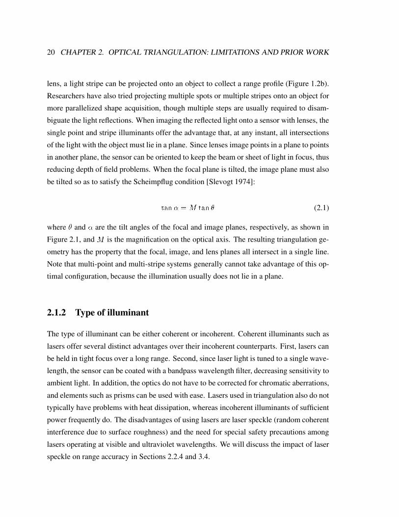
lens, a light stripe can be projected onto an object to collect a range profile (Figure 1.2b).
Researchers have also tried projecting multiple spots or multiple stripes onto an object for
more parallelized shape acquisition, though multiple steps are usually required to disam-
biguate the light reflections. When imaging the reflected light onto a sensor with lenses, the
single point and stripe illuminants offer the advantage that, at any instant, all intersections
of the light with the object must lie in a plane. Since lenses image points in a plane to points
in another plane, the sensor can be oriented to keep the beam or sheet of light in focus, thus
reducing depth of field problems. When the focal plane is tilted, the image plane must also
be tilted so as to satisfy the Scheimpflug condition [Slevogt 1974]:
tan� = M tan � (2.1)
where � and � are the tilt angles of the focal and image planes, respectively, as shown in
Figure 2.1, and M is the magnification on the optical axis. The resulting triangulation ge-
ometry has the property that the focal, image, and lens planes all intersect in a single line.
Note that multi-point and multi-stripe systems generally cannot take advantage of this op-
timal configuration, because the illumination usually does not lie in a plane.
2.1.2 Type of illuminant
The type of illuminant can be either coherent or incoherent. Coherent illuminants such as
lasers offer several distinct advantages over their incoherent counterparts. First, lasers can
be held in tight focus over a long range. Second, since laser light is tuned to a single wave-
length, the sensor can be coated with a bandpass wavelength filter, decreasing sensitivity to
ambient light. In addition, the optics do not have to be corrected for chromatic aberrations,
and elements such as prisms can be used with ease. Lasers used in triangulation also do not
typically have problems with heat dissipation, whereas incoherent illuminants of sufficient
power frequently do. The disadvantages of using lasers are laser speckle (random coherent
interference due to surface roughness) and the need for special safety precautions among
lasers operating at visible and ultraviolet wavelengths. We will discuss the impact of laser
speckle on range accuracy in Sections 2.2.4 and 3.4.

2.2. LIMITATIONS OF TRADITIONAL METHODS 21
2.1.3 Sensor
Sensors for optical triangulation systems also come in a variety of forms. For narrow
beam illumination, point (zero-dimensional) sensors such as photodiodes or line (one-
dimensional) sensors such as lateral effect photodiodes and linear array CCD’s are suffi-
cient, though point sensors must be scanned to provide another dimension. For light stripe,
multi-point, and multi-stripe systems, a two-dimensional sensor is necessary and typically
comes in the form of a CCD array, though point and line sensors can also be scanned to
provide the required dimensions.
2.1.4 Scanning method
The method of scanning an object is also a matter of choice. During a single range imaging
sweep, the illumination-sensor system can be stationary while a platform translates and ro-
tates the object through the field of view, or the object may be stationary while the scanner
moves. Alternatively, both the object and the scanning equipment may be stationary while
rotating mirrors sweep the illuminant and sensor viewing directions across the object. For
this latter scanning approach, the sensor viewpoint must sweep in synchrony with the illu-
minant to ensure that the sensor tracks the moving illuminant and keeps it in focus (see, for
example, [Rioux et al. 1987]). In addition, an optical triangulation scanner can collect range
data in continuous sweeps such that consecutive range points are adjacent in space (barring
surface discontinuities). Alternatively, the scanning may proceed in spatially disjoint steps
where the object moves an arbitrary amount relative to the scanner between acquisitions.
In Chapters 3 - 4, we will be concerned with scanners which perform continuous sweeps
or which move in small steps relative to the object, because these types of motion permit
correction of systematic artifacts.
2.2 Limitations of traditional methods
For optical triangulation systems, the accuracy of the range data depends on proper inter-
pretation of imaged light reflections. The most common approach is to reduce the problem
to one of finding the “center” of a one dimensional pulse, where the “center” refers to the

22 CHAPTER 2. OPTICAL TRIANGULATION: LIMITATIONS AND PRIOR WORK
position on the sensor which hopefully maps to the center of the illuminant. Typically, re-
searchers have opted for a statistic such as mean, median or peak of the imaged light as
representative of the center. Each of these statistics gives the correct answer when the sur-
face is perfectly planar. In this case, the sensor records a compressed or expanded image of
the illuminant’s shape, depending on the orientation of the surface with respect to the illu-
minant and sensor. The location of the center of the imaged pulse is not altered under these
circumstances.
2.2.1 Geometric intuition
The general accuracy of these statistics breaks down, however, whenever the surface per-
turbs the shape of the illuminant. Perturbations of the shape of the imaged illuminant occur
whenever:
� The surface reflectance varies.
� The surface geometry deviates from planarity.
� The light paths to the sensor are partially occluded.
� The light is coherent, and the surface is sufficiently rough to introduce laser speckle.
In Figures 2.2-2.4, we give examples of how the first three circumstances result in range
errors even for an ideal triangulation system with infinite sensor resolution and perfect cal-
ibration. For purposes of illustration, we omit the imaging optics of Figure 2.1 and treat the
sensor as one-dimensional and orthographic. Further, we assume an illuminant of Gaussian
cross-section, and we use the mean for determining the center of an imaged pulse. Figure 2.2
shows how a step reflectance discontinuity results in range points that do not lie on the sur-
face. A comparison of Figures 2.2a and 2.2b shows that the range error worsens with larger
reflectance steps. Figure 2.3 provides two examples of shape variations resulting in range
errors. Note that in Figure 2.3b, the center of the illuminant is not even striking a surface.
In this case, a measure of the center of the pulse results in a range value, when in fact the
correct answer is to return no range value whatever. Finally, Figure 2.4 shows the effect of

2.2. LIMITATIONS OF TRADITIONAL METHODS 23
Surface
Sensor
Illuminant
Surface
Sensor
Illuminant
(a) (b)
�1
�2
�1
�2
Rangepoint Range
point
Figure 2.2: Range errors due to reflectance discontinuities. (a) The change in reflectance from lightgray to dark gray distorts the image of the illuminant, perturbing the mean and resulting in an erro-neous range point. (b) Same as (a), but the reflectance step is larger, causing a larger range error.
Surface
Sensor
Illuminant
Surface
Sensor
Illuminant
(a) (b)
Rangepoint
Rangepoint
Figure 2.3: Range errors due to shape variations. (a) When reflecting off of the surfaces at the cornershown, the left half of the Gaussian is much more compressed than the right half. The result is a shiftin the mean and an erroneous range point. (b) When the illuminant falls off the edge of an object,the sensor images some light reflection. In this case, a range point is found where there is no surfaceat all along the center of the illuminant.

24 CHAPTER 2. OPTICAL TRIANGULATION: LIMITATIONS AND PRIOR WORK
Sensor
Illuminant
Surface
Rangepoint
Figure 2.4: Range error due to sensor occlusion. A portion of the light reflecting from the object isblocked before reaching the sensor. The mean yields an erroneous range point, even when the centerof the illuminant is not visible.
occluding the line of sight between the illuminated surface and the sensor. This range error
is very similar to the error encountered in Figure 2.3b.
The fourth source of range error is laser speckle, which arises when coherent laser illu-
mination bounces off of a surface that is rough compared to a wavelength [Goodman 1984].
The surface roughness introduces random variations in optical path lengths, causing a ran-
dom interference pattern throughout space and at the sensor. Figure 2.5 shows a photograph
of laser speckle arising from a rough surface1. For triangulation systems, the result is an
imaged pulse with a noise component that affects the mean pulse detection, causing range
errors even from a planar target (see Figure 2.6).
1Although optically smooth surfaces (i.e., mirrors) do not introduce laser speckle, they are also extremelyhard to measure. Mirrored surfaces only reflect light to the sensor when the surface is properly oriented. Fur-ther, mirrored surfaces generally result in interreflections that significantly complicate range analysis. As aresult, diffusely reflecting surfaces are desirable for range scanning. Diffuseness arises from surface rough-ness, which in turn leads to laser speckle.

2.2. LIMITATIONS OF TRADITIONAL METHODS 25
Figure 2.5: Image of a rough object formed with coherent light. Source: [Goodman 1984].
�ci
�r
Laser Sensor
Surface
Lens
Aperture
Figure 2.6: Influence of laser speckle on traditional triangulation. The image of the Gaussian is noisy,causing a random shift in the position of the mean, ci. The uncertainty in the mean’s position, �cimaps to an uncertainty in the observed range, �r. Note that the direction of range uncertainty followsthe center of the laser beam.

26 CHAPTER 2. OPTICAL TRIANGULATION: LIMITATIONS AND PRIOR WORK
theta = 10 deg theta = 20 deg theta = 30 deg theta = 40 deg
|1
|2
|3
|4
|5
|6
|7
|8
|9
|10
|0.0
|0.5
|1.0
|1.5
|2.0
|2.5
|3.0
Reflectance Ratio
Max
Err
or /
Las
er W
idth
Figure 2.7: Plot of errors due to reflectance discontinuities. As the size of the reflectance step (rep-resented as the ratio of reflectances on either side of the step), the deviation from planarity increasesaccordingly. Smaller triangulation angles (theta) exhibit greater errors.
2.2.2 Quantifying the error
To quantify the errors inherent in using traditional mean analysis, we numerically computed
the errors introduced by reflectance and shape variations for an ideal triangulation system
with a single Gaussian illuminant. We define the normally incident irradiance profile of the
Gaussian illuminant as:
EL(x) = IL exp
"�2x2w2
#(2.2)
where IL is the power of the beam at its center, and w is a measure of beam width, taken to
be the distance between the beam center and the e�2 point. This measure of beam width is
common in the optics literature. We present the range errors in a scale invariant form by di-
viding all distances by the beam width. Figure 2.7 illustrates the maximum deviation from
planarity introduced by scanning a reflectance discontinuity of varying step magnitudes for
four different triangulation angles. As the size of the step increases, the error increases cor-
respondingly. In addition, smaller triangulation angles, which are desirable for reducing the
likelihood of missing data due to sensor occlusions, actually result in larger range errors.

2.2. LIMITATIONS OF TRADITIONAL METHODS 27
|60
|80
|100
|120
|140
|160
|180
|0.00
|0.25
|0.50
|0.75
|1.00
|1.25
|1.50
Corner Angle (Degrees)
Clo
sest
Dis
tanc
e / L
aser
Wid
th
Figure 2.8: Plot of errors due to corners. The y-axis indicates the closest distance between the rangedata and the actual corner, while the x-axis measures the angle of the corner. Tighter corners resultin greater range errors.
This result is not surprising, as sensor mean positions are converted to depths through a di-
vision by sin �, where � is the triangulation angle, so that errors in mean detection translate
to larger range errors for smaller triangulation angles.
Figure 2.8 shows the effects of a corner on range error, where the error is taken to be the
shortest distance between the computed range data and the exact corner point. The corner is
oriented so that the illumination direction bisects the corner’s angle as shown in Figure 2.3a.
As we might expect, a sharper corner results in greater compression of the left side of the
imaged Gaussian relative to the right side, pushing the mean further to the right on the sensor
and pushing the triangulated point further behind the corner. In this case, the triangulation
angle has little effect as the greater mean error to depth error amplification is offset almost
exactly by the smaller observed left/right pulse compression imbalance.
We can estimate what the absolute values of these errors are for a typical triangulation
system. For example, the triangulation angle of our scanner hardware is 30o, and the laser
width is about 1 mm across a depth of 0.3 m. For this configuration, we would expect errors
of 0.8 mm for a 10:1 reflectance step and 0.5 mm for a corner angle of 110o.

28 CHAPTER 2. OPTICAL TRIANGULATION: LIMITATIONS AND PRIOR WORK
z
wo
zR
p2wo
wopt(z)wnar(z)
wwide(z)Lens
Collimatedbeam
zD
Figure 2.9: Gaussian beam optics. A collimated beam is focused by the lens to a width, wo, andspans a desired depth of field zD. Bringing the beam into tight focus results in a rapidly expandingbeam (wnar (z)). A wide beam expands slowly (wwide(z)), but may be too wide over the desireddepth of field. The optimal beam (wopt(z)) expands only by a factor of
p2 over the depth of field.
For this optimal configuration, the distance between the beam waist and thep2 point is called the
Rayleigh range, zR.
2.2.3 Focusing the beam
One possible strategy for reducing the errors described in the previous section is to narrow
the illuminating beam. Unfortunately, there are practical limitations to implementing this
strategy. First, in order to take advantage of the smaller beam width, the sensor resolution
must increase. This leads to expensive sensors. Second, using lenses to focus a Gaussian
beam arbitrarily over the field of view is not possible due to diffraction limits. The best
candidate for a tightly focused illuminant over a large depth of field is a laser beam. The
irradiance profile of a laser beam is typically Gaussian as described by Equation 2.2, and
the width of the beam expands from its narrowest point as [Siegman 1986]:
w(z) = wo
vuut1 +
�z
�w2o
!2
wherewo is the beam waist or width of the beam at its narrowest point, z is the distance from
this point, and � is the wavelength of the laser. Figure 2.9 shows how the beam expands for
various beam waists. Note that as the waist becomes narrower, the beam expands faster. For
a given depth of field, zD, we want the beam to be as tight as possible to limit the effects
of triangulation errors. If the waist is too narrow, then the beam expands too rapidly and
becomes too large at the edges of the field of view. If the waist is too large, it expands slowly,

2.2. LIMITATIONS OF TRADITIONAL METHODS 29
but is still too large at the edges of the field of view. The optimum beam width is attained
when the waist obeys the relation:
wo =
s�zD2�
In this case, the beam reaches a maximum width ofw =p2wo and the value zR = zD=2
corresponds to what is known as the Rayleigh range of the beam. The variation in width is
thus:
s�zD2�� w �
s�zD�
The best width to range ratio at the edges of the field of view is:
w
zD=
s�
�zD(2.3)
The discussion of range errors due to reflectance and shape variations in the previous
section shows that the errors of an optical triangulation system are on the order of the width
of the illuminant. Thus, the beam width to range ratio is a measure of the relative accuracy
of the system. Equation 2.3 tells us that once we have selected a range of interest, diffrac-
tion limits impose a bound on the relative accuracy in the presence of reflectance and shape
variations.
Note that Bickel et al. [1985] have explored the use of axicons (e.g., glass cones and
other surfaces of revolution) to attain tighter focus of a Gaussian beam. The refracted beam,
however, has a zeroth order Bessel function cross-section; i.e., it has numerous side-lobes
of non-negligible irradiance. The influence of these side-lobes is not well-documented and
would seem to complicate triangulation. In addition, once the sensor resolution is fixed,
then arbitrarily narrowing the beam actually becomes undesirable. If the image of the beam
spans only one or two pixels, then the computed mean will not attain sub-pixel accuracy.
See Section 3.5 for a discussion of the beam width in a signal processing context.
30 CHAPTER 2. OPTICAL TRIANGULATION: LIMITATIONS AND PRIOR WORK
2.2.4 Influence of laser speckle
Even under the most ideal circumstances of scanning a planar object with no reflectance
variations, the accuracy of optical triangulation methods using coherent illumination are
still limited by an unavoidable interference phenomenon: laser speckle. In this section, we
describe how laser speckle arises and how it results in range errors.
In order to analyze the effects of laser speckle, we must consider the wave nature of
light and, in particular, the effects of diffraction. One of the most powerful tools for study-
ing these effects is scalar diffraction theory. Scalar diffraction theory treats light as a scalar
field rather than as a coupled electric and magnetic field. Experiment has shown that this
approximation is valid as long as (1) the diffracting aperture is large compared to a wave-
length and (2) the diffracted fields are not being observed too close to the aperture. Both of
these criteria are satisfied in the current context.
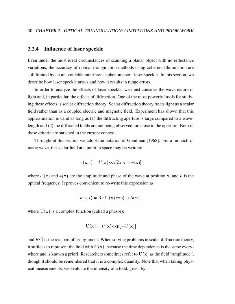
Throughout this section we adopt the notation of Goodman [1968]. For a monochro-
matic wave, the scalar field at a point in space may be written:
u(x; t) = U(x) cos[2��t+ �(x)]
where U(x) and �(x) are the amplitude and phase of the wave at position x, and � is the
optical frequency. It proves convenient to re-write this expression as:
u(x; t) = Re[U(x) exp(�i2��t)]
where U(x) is a complex function (called a phasor):
U(x) = U(x) exp[�i�(x)]
andRe[] is the real part of its argument. When solving problems in scalar diffraction theory,
it suffices to represent the field with U(x), because the time dependence is the same every-
where and is known a priori. Researchers sometimes refer toU(x) as the field “amplitude”,
though it should be remembered that it is a complex quantity. Note that when taking phys-
ical measurements, we evaluate the intensity of a field, given by:

2.2. LIMITATIONS OF TRADITIONAL METHODS 31
xo
yo
do di
x
y
xi
yi
a
LensAperture
Image plane
Object Planez
Figure 2.10: Imaging geometry and coordinate systems.
I(x) = jU(x)j2 = U(x)U�(x)
Now consider the imaging geometry shown in Figure 2.10. A striking result from scalar
diffraction theory is the fact that the image formed by a lens is the same as the image de-
scribed by geometrical optics, filtered by an amplitude spread function (also known as a
point spread function):
Ui(xi; yi) = Ug(xi; yi) � h(xi; yi) (2.4)
where Ui is the resulting image field, and Ug is the geometrical optics image, which is in
turn given by the relation:
Ug(xi; yi) =1
MUo
�� xiM
;� yiM
�(2.5)
where Uo is the field in the object plane, and M is the magnification factor. The amplitude
spread function is simply the Fourier transform of the lens pupil:
h(xi; yi) =Z Z
1
�1
P (�disx; �disy) exp[�i2�(xisx + yisy)]dsxdsy (2.6)
where P (x; y) describes the shape of the pupil (usually a circular disc), di is the distance to
the image, and � is the optical wavelength. For a circular lens aperture, the pupil function is
unity with a radius of a and zero outside. The amplitude spread function for such an aperture
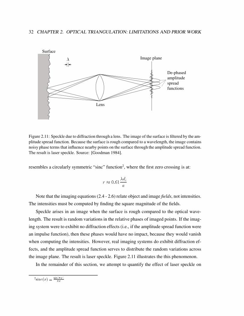
32 CHAPTER 2. OPTICAL TRIANGULATION: LIMITATIONS AND PRIOR WORK
Surface
Lens
Image plane
De-phasedamplitudespreadfunctions
�
Figure 2.11: Speckle due to diffraction through a lens. The image of the surface is filtered by the am-plitude spread function. Because the surface is rough compared to a wavelength, the image containsnoisy phase terms that influence nearby points on the surface through the amplitude spread function.The result is laser speckle. Source: [Goodman 1984].
resembles a circularly symmetric “sinc” function2, where the first zero crossing is at:
r � 0:61�dia
Note that the imaging equations (2.4 - 2.6) relate object and image fields, not intensities.
The intensities must be computed by finding the square magnitude of the fields.
Speckle arises in an image when the surface is rough compared to the optical wave-
length. The result is random variations in the relative phases of imaged points. If the imag-
ing system were to exhibit no diffraction effects (i.e., if the amplitude spread function were
an impulse function), then these phases would have no impact, because they would vanish
when computing the intensities. However, real imaging systems do exhibit diffraction ef-
fects, and the amplitude spread function serves to distribute the random variations across
the image plane. The result is laser speckle. Figure 2.11 illustrates the this phenomenon.
In the remainder of this section, we attempt to quantify the effect of laser speckle on
2sinc(x) � sin(�x)�x

2.2. LIMITATIONS OF TRADITIONAL METHODS 33
range accuracy. To do so, we consider the case of a two-dimensional world, which permits
us to remove references to the y coordinate in the equations above. This simplification will
aid in the discussion of the issues of laser speckle, but will not significantly alter the ba-
sic results. Note that in this two-dimensional world, the amplitude spread function for an
imaging aperture is simply the “sinc” function. In addition, we will treat the triangulation
imaging geometry as though it were an axially aligned imaging geometry. This approxima-
tion introduces some error, because some of the imaged light originates from regions outside
of the plane in focus (the center of the illuminant), but for narrow illuminants, this error is
negligible [Francon 1979].
For a Gaussian illuminant incident on the surface of an object, the field at the surface of
the object takes the form:
Uo(xo) = Go(xo) exp[i�o(xo)] (2.7)
whereGo(xo) is the Gaussian illuminant and �o(xo) represents the random phase variations
introduced by the roughness of the surface. We can now write the field at the image plane
as:
Ui(xi) = fGg(xi) exp[i�g(xi)]g � h(xi)
where Gg(xi) and �g(xi) are the images of the Gaussian and and phase terms, respectively,
as given by geometric optics. From this equation, we can compute the intensity measured
at the image plane:
Ii(xi) = Ui(xi)U�
i (xi) (2.8)
Equations 2.7 - 2.8 describe the physical image of a Gaussian illuminant after experi-
encing random phase variations and diffraction “filtering.” Errors in determining the mean
of this image result in range errors in triangulation systems using traditional analysis. The
mean is defined by:

34 CHAPTER 2. OPTICAL TRIANGULATION: LIMITATIONS AND PRIOR WORK
ci =
Z1
�1
xiIi(xi)dxiZ1
�1
Ii(xi)dxi(2.9)
For a centered Gaussian, this mean should be exactly zero; however, the random phase vari-
ations introduce statistical variations in the mean that we can quantify as:
�ci = [hc2i i � hcii2]1
2 = hc2i i1
2 (2.10)
where the expected value of the mean is assumed to be zero. Figure 2.6 illustrates the influ-
ence of laser speckle in a triangulation system. The error in the mean maps to a range error
through the relation:
�r =M�cisin �
In other words, once we have computed the variations in detecting the mean at the sensor, we
must map it into a range error through multiplication by the imaging system’s magnification
factor, M , and division by the triangulation factor, sin �.
Computing the standard deviation described by Equations 2.9 and 2.10 analytically has
proven to be extremely difficult. Instead, we have performed numerical simulations. These
simulations require some characterization of the phase function, �o(xo), which describes
the roughness of the surface. Researchers typically model this function to be proportional
to the height profile, �(xo) of the surface:
�o(xo) =2�
��(xo)
This �(xo) is typically taken to be a random process with Gaussian statistics at each
point on the surface and a Gaussian autocorrelation spectrum. The pointwise statistics are
thus parameterized by the surface height variance, Rq, also called the roughness, and the
correlation length, � [Fujii et al. 1976]. As a result, the parameter space we must explore is
four dimensional: a function of the width of the laser, the width of the point spread function,
the surface roughness and the correlation length. To date, we have thoroughly studied the

2.2. LIMITATIONS OF TRADITIONAL METHODS 35
deviation of the mean for surfaces rough compared to a wavelength with zero correlation
length, and we have arrived at a qualitative understanding of the behavior when the surface
roughness parameters are varied. For uncorrelated rough surfaces, the variation of the mean
follows the relation:
�ci �1
2
swi�di2a
where wi is the width of the image of the Gaussian illuminant, di is the distance from the
lens to the aperture, and a is the aperture radius. Mapping this into a range error we obtain:
�r � M
2 sin �
swi�di2a
Noting that w = Mwi is the width of the illuminant in object space, and do = Mdi is the
distance to the object, the range error can be re-written as:
�r � 1
2 sin �
sw�do2a
(2.11)
This relation yields several insights. First of all, the range error is fundamentally indepen-
dent of the resolution of the sensor; it is an inescapable consequence of the speckle phe-
nomenon. Secondly, we expect that narrowing the aperture will increase the speckle noise
and thereby increase the range error. Finally, the range error varies with the square root of
the width of the laser as seen from the sensor. Narrowing the laser ought to decrease range
noise.
Numerical experiments with various surface roughness and correlation length parame-
ters have yielded some quantitative results that follow qualitative expectations. In summary,
as the correlation length grows, we observe a decrease in the computed range error. Simi-
larly, as the surface roughness decreases, the range error also decreases. This result is not
surprising; the limiting case of a perfectly smooth planar surface should result in no laser
speckle and thus no range error. Increasing the correlation length and decreasing the rough-
ness bring the results closer to the perfectly smooth case.
To give a sense for the size of the range errors, we can substitute some typical values
into Equation 2.11. The triangulation system used for experiments in Chapter 4 has a 30

36 CHAPTER 2. OPTICAL TRIANGULATION: LIMITATIONS AND PRIOR WORK
degree triangulation angle, an aperture radius of about 5 mm, a stand-off of 1 meter and
uses a HeNe laser source (� = 632.8 nm). We would therefore expect the range error due
to reflections from a “perfectly” rough surface to be approximately 0.25 mm. This error
corresponds to roughly half the resolution of the sensor being used. Real surfaces, however,
are not perfectly rough, so we would expect smaller range errors in practice.
2.3 Prior work on triangulation error
Several researchers have observed the limitations in triangulation accuracy due to re-
flectance and shape variations [Buzinski et al. 1992] [Soucy et al. 1990] [Mundy & Porter
1987]. In addition, researchers have studied the effect of laser speckle on range determi-
nation and have indicated that speckle is a fundamental limit to the accuracy of laser range
triangulation, as described in the previous section, though its effects can be reduced with
well-known speckle reduction techniques [Baribeau & Rioux 1991] [Dorsch et al. 1994].
These speckle reduction methods, however, typically require spatial averaging, resulting in
a trade-off between noise and spatial resolution. Using a less coherent light source appears
to be a better alternative, as it leads to less speckle noise without loss of resolution. Re-
gardless, changing the viewpoint generally results in a different speckle pattern, so multiple
range images acquired from different viewpoints can be combined to reduce noise without
loss of resolution. We demonstrate this last idea in Section 8.3.
Mundy & Porter [1987] attempt to correct for variations in surface reflectance by noting
that two imaged pulses, differing in position or wavelength are sufficient to overcome the
reflectance errors on a planar surface, though some restrictive assumptions are necessary for
the case of differing wavelengths, and they do not address errors due to shape variations.
Kanade et al. [1991] describe a rangefinder that finds peaks in time for a stationary sensor
with pixels that view fixed points on an object as the illuminant sweeps across the scene.
This method is very similar to the spacetime analysis presented in this thesis for solving
some of the problems of optical triangulation; however, the authors in [Kanade et al. 1991]
do not indicate awareness that their design addresses these problems. Further, we show that
the principle generalizes to other scanning geometries.

2.3. PRIOR WORK ON TRIANGULATION ERROR 37

Chapter 3
Spacetime Analysis
Many optical triangulation scanners operate by sweeping the illumination over an object
while imaging the reflected light over time. The previous chapter clearly demonstrates that
analyzing the imaged pulses at each time step leads to systematic range errors. In this chap-
ter, we describe a new method for optical triangulation called spacetime analysis. We show
that by analyzing the time evolution of the imaged pulses, this new method can reduce or
eliminate range errors associated with traditional methods.
We begin with an intuitive description of how the spacetime analysis works (Sec-
tion 3.1), followed by a rigorous derivation of its properties under a set of assumptions such
as linear scanning and orthographic sensing (Section 3.2). We then describe how the method
generalizes when weakening or removing these assumptions (Section 3.3). In Section 3.4,
we consider the role of laser speckle in spacetime analysis and show that it still imposes a
limit on triangulation accuracy. Finally, we put optical triangulation scanners into a signal
processing context and draw conclusions about how to improve them (Section 3.5).
3.1 Geometric intuition
Figure 3.1 illustrates the principle of spacetime analysis for a laser triangulation scanner
with Gaussian illuminant and orthographic sensor as it translates across the edge of an ob-
ject. As the scanner steps to the right, the sensor images a smaller and smaller portion of the
laser cross-section. By time t3, the sensor no longer images the center of the illuminant, and
38

3.1. GEOMETRIC INTUITION 39
Illuminant
Sensor
Surface
t1
t2
t3
t4
tc
v(tc; sc)
(xc; zc)
t1 t2 tc t3 t4
Figure 3.1: Spacetime mapping of a Gaussian illuminant. The Gaussians at left represent the profileof the illuminant at times t1 through t4. The solid Gaussians at right represent the images of theilluminant at these same times. The dashed Gaussian represents the time evolution of these imagesfor a single line of sight, corresponding to a single point on the targeted surface. Although the solidGaussians at right may be distorted or clipped by depth discontinuities or reflectance changes in thesurface, the dashed Gaussian is always the same shape (unless it is missing entirely), and it is centeredat a location that corresponds exactly to a range point. These properties of the dashed Gaussian arethe keys to the spacetime analysis.
conventional methods of range estimation fail. However, if we look along the lines of sight
from the corner to the laser and from the corner to the sensor, we see that the profile of the
laser is being imaged over time onto the sensor (indicated by the dotted Gaussian envelope).
Thus, we can find the coordinates of the corner point (xc; zc) by searching for the mean of
a Gaussian along a constant line of sight through the sensor images. We can express the
coordinates of this mean as a time and a position on the sensor, where the time is in general
between sensor frames and the position is between sensor pixels. The position on the sensor
indicates a depth, and the time indicates the lateral position of the center of the illuminant.
In the example of Figure 3.1, we find that the spacetime Gaussian corresponding to the exact
corner has its mean at position sc on the sensor at a time tc between t2 and t3 during the scan.
We establish the corner’s position by triangulating the center of the illuminant at time tc

40 CHAPTER 3. SPACETIME ANALYSIS
s
Illuminant
Sensor
Surface
�
p
v
n!L
z�O
x!S
Figure 3.2: Triangulation scanner coordinate system.
with the sensor line of sight corresponding to the sensor coordinate sc and the lateral sensor
position at tc.
3.2 A complete derivation
For a more rigorous analysis, we consider the time evolution of the irradiance from a trans-
lating differential surface element, �O, as recorded at the sensor. We refer the reader to
Figure 3.2 and Table 3.1 for a description of coordinate systems and symbols. Note that in
contrast to the previous section, the surface element is translating instead of the illuminant-
sensor assembly. The element has a normal n and an initial position po and is translating
with velocity v, so that:
p(t) = po + tv
Our objective is to compute the coordinates po = (xo; zo) given the temporal irradiance
variations on the sensor. For simplicity, we assume that v = (�v; 0). The illuminant we
consider is a laser with a unidirectional Gaussian radiance profile:
LL(x;!) = IL exp
"�2x2w2
#�(! � !L) (3.1)

3.2. A COMPLETE DERIVATION 41
�O Differential surface elementp(t) Position of surface elementpo Position of surface element (xo; zo) at time t = 0n Normal of surface elementv Velocity of whole object!L Direction of illuminant!S View direction
Table 3.1: Symbol definitions for spacetime analysis.
where IL is the power of the beam at its center,w is the e�2 half width, and the delta function
indicates the directionality of the beam. In accordance with Figure 3.2, we will assume that
!L = (0; 1). The differential reflected radiance from the element in the direction of the
sensor is simply:
dL(p(t);!S) = fr(!;!S)jn � !LjLL(p(t);!)d! (3.2)
where fr(!;!S) is the bidirectional reflection distribution function (BRDF) of the pointpo,
evaluated at the incident direction, !, and outgoing sensor direction, !S . Note that we as-
sume that the BRDF is defined in a global sense for the surface element, rather than relative
to its normal. Further, we treat incoming directions as pointing toward the surface rather
than away from the surface, which is consistent with the description of the radiance field in
terms of position and direction.
Substituting Equation 3.1 into Equation 3.2 and integrating over all incident directions,
we find the total radiance reflected from the element to the sensor to be:
L(p(t);!S) = fr(!L;!S)jn � !LjIL exp"�2(xo � vt)2
w2
#(3.3)
Projecting the point p(t) onto the sensor, we find:
s = (xo � vt) cos � � zo sin � (3.4)

42 CHAPTER 3. SPACETIME ANALYSIS
x
z
zo
xo
�
�LS IL
w0=
wsin �
ES
Figure 3.3: Spacetime image of the Gaussian illuminant. After scaling the sensor scanlines to mapto depth and lateral displacement, we see that a point is imaged to a tilted Gaussian in the spacetimeimage. The center of the Gaussian maps to the coordinates of the point, the amplitude depends onthe reflectance coefficient and beam strength, and the width is fixed by the scanner geometry.
where s is the position on the sensor and � is the angle between the sensor and laser direc-
tions. We combine Equations 3.3-3.4 to give us an equation for the irradiance observed at
the sensor as a function of time and position on the sensor:
ES(t; s) = fr(!L;!S)jn � !LjIL exp"�2(xo � vt)2
w2
#�(s� (xo � vt) cos � � zo sin �)
To simplify this expression, we condense the light reflection terms into one measure:
�LS = fr(!L;!S)jn �!Lj
which we will refer to as the reflectance coefficient of point p. We also note that x = vt
is a measure of the relative x-displacement of the point during a scan, and z = s= sin � is
the relation between sensor coordinates and depth values along the center of the illuminant.
Making these substitutions we have:
ES(x; z) = �LSIL exp
"�2(x� xo)2
w2
#�((x� xo) cos � + (z � zo) sin �) (3.5)

3.2. A COMPLETE DERIVATION 43
(a)(b) (c) (d)
TA SA
Illuminant
Sensor
Figure 3.4: From geometry to spacetime image to range data. (a) The original geometry. (b) Theresulting spacetime image. TA indicates the direction of traditional analysis, while SA is the direc-tion of the spacetime analysis. The dotted line corresponds to the scanline generated at the instantshown in (a). (c) Range data after traditional mean analysis. (d) Range data after spacetime analysis.
This equation describes a Gaussian running along a tilted line through the spacetime
sensor plane or spacetime image as depicted in Figure 3.3. We define the spacetime image to
be the image whose columns are filled with sensor scanlines that evolve over time. Through
the substitutions above, position within a column of this image represents displacement in
depth, and position within a row represents time or displacement in lateral position. From
Figure 3.3, we see that the tilt angle is � with respect to the z-axis, and the width of the
Gaussian along the line is:
w0 =w
sin �
The peak value of the Gaussian is �LSIL, and its mean along the line is located at (xo; zo),
the exact location of the range point. Note that the angle of the line and the width of the
Gaussian are solely determined by the fixed parameters of the scanner, not the position, ori-
entation, or BRDF of the surface element. Thus, extraction of range points should proceed
by computing low order statistics along tilted lines through the spacetime image, rather than
along columns (scanlines) as in the conventional method. Figure 3.4 illustrates this distinc-
tion. Further, we establish the position of the surface element independent of the orienta-
tion and BRDF of the element and, assuming no interreflections, independent of any other
nearby surface elements. The decoupling of range determination from local shape and re-
flectance is complete. As a side effect, the peak of the Gaussian yields the irradiance at the
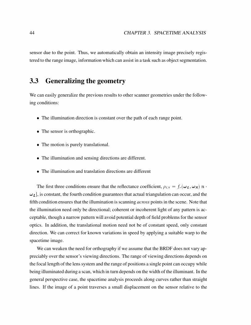
44 CHAPTER 3. SPACETIME ANALYSIS
sensor due to the point. Thus, we automatically obtain an intensity image precisely regis-
tered to the range image, information which can assist in a task such as object segmentation.
3.3 Generalizing the geometry
We can easily generalize the previous results to other scanner geometries under the follow-
ing conditions:
� The illumination direction is constant over the path of each range point.
� The sensor is orthographic.
� The motion is purely translational.
� The illumination and sensing directions are different.
� The illumination and translation directions are different
The first three conditions ensure that the reflectance coefficient, �LS = fr(!L;!S)jn �!Lj, is constant, the fourth condition guarantees that actual triangulation can occur, and the
fifth condition ensures that the illumination is scanning across points in the scene. Note that
the illumination need only be directional; coherent or incoherent light of any pattern is ac-
ceptable, though a narrow pattern will avoid potential depth of field problems for the sensor
optics. In addition, the translational motion need not be of constant speed, only constant
direction. We can correct for known variations in speed by applying a suitable warp to the
spacetime image.
We can weaken the need for orthography if we assume that the BRDF does not vary ap-
preciably over the sensor’s viewing directions. The range of viewing directions depends on
the focal length of the lens system and the range of positions a single point can occupy while
being illuminated during a scan, which in turn depends on the width of the illuminant. In the
general perspective case, the spacetime analysis proceeds along curves rather than straight
lines. If the image of a point traverses a small displacement on the sensor relative to the

3.3. GENERALIZING THE GEOMETRY 45
focal length, then assumption of local orthography is reasonable. In addition, general per-
spective can lead to changes in occlusion relationships during a scan that cause an illumi-
nated point to be visible for a finite time and then become invisible while still illuminated.
This effect results in a partial image of the occluded point’s spacetime Gaussian and will
result in a range error for this point. These points will be easy to identify: they will be near
step discontinuities in the resulting range image. When acquiring multiple range images,
these points can be eliminated in favor of unoccluded acquisitions of the same portions of
the surface. Thus, while perspective sensors can create some complications in applying the
spacetime analysis, typical lens configurations will yield reasonable results.
We can also weaken the requirement for pure translation, as long as the rotational com-
ponent of motion represents a small change in direction with respect to the fr(!L;!S)jn �!Lj product. This constraint is reasonable for motion trajectories with large radii of curva-
ture relative to the beam width. As in the perspective case, the spacetime analysis proceeds
in general along curves, and changes in occlusion relationships can lead to erroneous range
data. Nonetheless, for moderate rotational trajectories, the spacetime analysis will lead to
improved range data.

46 CHAPTER 3. SPACETIME ANALYSIS
3.4 Influence of laser speckle
In the previous chapter, we developed the equations that are needed to analyze the influence
of laser speckle on range determination. The results of statistical analysis show that laser
speckle places a limit on the attainable accuracy when using traditional triangulation. Does
spacetime analysis eliminate this limitation? One encouraging observation is the fact that
the imaging equation (2.4) is space-invariant, so that moving the object field corresponds
to moving the image field. In this way, speckle behaves as though it adheres to the sur-
face, much like a noisy reflectance variation. This observation would seem to indicate that
the spacetime analysis would correct for speckle noise. However, when we move the object
with respect to a non-uniform illuminant (such as a laser beam with Gaussian cross-section),
then the object field is not simply translating. As a result, the speckle does not completely
adhere to the surface, and spacetime analysis faces the same limitation as traditional trian-
gulation: laser speckle imposes a fundamental limit on accuracy. In this section, we will
develop some of the equations necessary to demonstrate this result.
For the spacetime analysis, we must consider a moving surface and follow a single point
on the surface to observe the image of the Gaussian mapped over time. Conversely, we can
consider a moving illuminant, and follow a single line of sight from a stationary sensor.
These two cases are equivalent as far as the resulting speckle patterns are concerned, but
the latter yields a simpler analysis.
We can describe the field at the surface of the object in terms of the moving illuminant:
Uo(xo; t) = Go(xo � vot) exp[i�o(xo)]
where the Gaussian is moving with velocity vo. Mapping this to the image plane:
Ui(xi; t) = fGg(xi � vit) exp[i�g(xi)]g � h(xi)
where Gg and �g are the images of the Gaussian and phase functions given by geometric
optics, and vi is the velocity of the imaged Gaussian. To simplify this relation, we can first
expand the convolution:

3.4. INFLUENCE OF LASER SPECKLE 47
Ui(xi; t) =Z1
�1
Gg(xi � vit� �) exp[i�g(xi � �)]h(�)d�
Next, we consider a single line of sight, xi = 0, so that:
Ui(0; t) =Z1
�1
Gg(�vit� �) exp[i�g(��)]h(�)d�
For a symmetric amplitude spread function, and after some straightforward manipulations,
this relation becomes:
Ui(0; t) = Gg(�) � fexp[i�g(�)]h(�)g j�=vit (3.6)
As described in the previous chapter, the intensity is the square magnitude of the field,
but in this case, the mean we seek is with respect to time:
ct =
Z1
�1
tIi(0; t)dtZ1
�1
Ii(0; t)dt(3.7)
The error can be solved as the variance of the mean as described in the previous chapter:
�ct = [hc2t i � hcti2]1
2 = hc2t i1
2 (3.8)
Figure 3.5 illustrates the influence of laser speckle when using spacetime triangulation.
For traditional analysis, the uncertainty in the position of the mean on a sensor scanline cor-
responds directly to a depth error along the center of the illuminant. For spacetime triangu-
lation, the error in the mean maps to an error in determining when the laser sheet’s center
intersects a line of sight at a range point. The range error is distributed along the sensor’s
line of sight, and obeys the relation:
�r =vo�ctsin �
(3.9)

48 CHAPTER 3. SPACETIME ANALYSIS
�ct
�r
LaserSensor
Surface
t
Lens
�ct
Figure 3.5: Influence of laser speckle on spacetime triangulation. When performing the spacetimeanalysis, the line of sight to the point is fixed, but the time at which the center of the laser passes overthe range point varies with range. Laser speckle introduces uncertainty, �ct as to when the laser iscentered over the range point. The effect is range uncertainty, �r, along the line of sight from thesensor.
As in the case for traditional analysis, computing an analytical solution using Equa-
tions 3.6-3.9 has proven to be extremely difficult. Instead, we have performed numeri-
cal simulations that lead us to the same result as we found for traditional analysis (Equa-
tion 2.11):
�r � 1
2 sin �
sw�do2a
(3.10)
Thus, the error in spacetime triangulation under coherent illumination is independent of
sensor resolution and increases with the narrowing of the aperture and the widening of the
laser sheet. In addition, numerical analysis reveals that, just as in the case for traditional
triangulation, smoother surfaces lead to reductions in range error.

3.4. INFLUENCE OF LASER SPECKLE 49
(a) (b) (c)
Sensor
Surface
Fixed
t1 t2 t3 t4LaserMoving
Figure 3.6: Speckle contributions at the sensor due to a moving coherent illuminant with squarecross-section. The sensor and surface are stationary while the illuminant sweeps across the surface.A single pixel maps to a single point on the surface, but a neighborhood of points on the surface in-fluence the pixel intensity as a result of diffraction at the aperture. This neighborhood is indicated bythe region between the lines drawn from the sensor to the surface. (a) As the illumination translatesto the right (shown here at time t1), only part of the neighboring points, mostly to the left of the rangepoint, are illuminated. Only these points will contribute to the observed, speckle-corrupted intensityat the sensor. (b) At time t2, the illumination uniformly covers the neighborhood and continues to doso until time t3. During this time, the pixel intensity will not vary as the illumination moves. (c) Asthe left edge of the illumination crosses into the neighborhood near the range point (shown here attime t4), then only the the points mostly to the right of the range point will affect the pixel intensity.Thus, we expect the speckle noise in (a) and (c) to be uncorrelated.
The impact of laser speckle on traditional triangulation is not surprising, given the obvi-
ous corruption of the imaged illuminant. The effect of speckle on spacetime triangulation,
however, is harder to visualize. To gain a more intuitive grasp, consider the example in Fig-
ure 3.6, which illustrates the didactic example of a stationary object and sensor and a moving
illuminant with square irradiance profile. A single pixel on the sensor maps to a single point
on the surface, but due to diffraction at the aperture, neighboring points on the surface influ-
ence the intensity measured at this pixel. When the sensor approaches the range point from
the left, then surface points to the left of the range point affect the pixel intensity. When the
illumination is completely covering the neighborhood of the range point, then translations
of the illuminant do not affect the measured intensity. As the illumination passes the range
point to the right, the surface points to the right of the range point affect the pixel intensity.
Thus, when the illuminant is mostly to the left or right of the range point, the pixel intensity
is determined by different points on the surface.

50 CHAPTER 3. SPACETIME ANALYSIS
(a) (b)
Laser
Sensor
�ct
�r
Surface
I
t
�1 �2
Figure 3.7: Spacetime speckle error for a coherent illuminant with square cross-section. (a) As thesensor and illuminant sweep over the surface, the sensor images noisy square waves. For regionsnear the center of the square wave, the speckle behaves as though it adheres to the surface as thescanning progresses. Near the edges, however, the speckle influence reveals itself. For the rangepoint being tracked, the amplitude in the first image depends on the properties of the left portion ofthe surface, while the amplitude in the last image depends on the right portion of the surface. In (b)we see the resulting spacetime image of the range point. The central regions of the pulse are veryflat, unlike the individual images of the square pulse at each time step in (a). However, the speckleinfluences the edges of the pulse, resulting in uncertainty about the mean of the pulse.
Figure 3.7 illustrates how this distinction leads to errors in spacetime triangulation, this
time including the motion of the sensor along with the illuminant. As the center of the square
illuminant moves over the object, the speckled image of the surface does indeed move with
the surface, because the illuminant is fairly constant near the center. This explains why the
spacetime pulse is very flat in the center (Figure 3.7b). However, near the edges of the pulse,
the illumination is not at all constant, and speckle noise appears. The result is an uncertainty
in determining the location of these edges. The noise at the edges has different properties
for the left edge versus the right edge as described above, meaning that the uncertainty in
determining the position of the two edges is fairly uncorrelated. Since resolving the edges
is the only way of determining the center of the spacetime pulse, spacetime triangulation is
limited in accuracy by laser speckle.
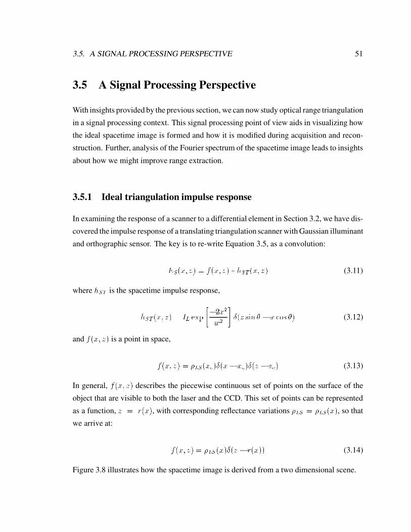
3.5. A SIGNAL PROCESSING PERSPECTIVE 51
3.5 A Signal Processing Perspective
With insights provided by the previous section, we can now study optical range triangulation
in a signal processing context. This signal processing point of view aids in visualizing how
the ideal spacetime image is formed and how it is modified during acquisition and recon-
struction. Further, analysis of the Fourier spectrum of the spacetime image leads to insights
about how we might improve range extraction.
3.5.1 Ideal triangulation impulse response
In examining the response of a scanner to a differential element in Section 3.2, we have dis-
covered the impulse response of a translating triangulation scanner with Gaussian illuminant
and orthographic sensor. The key is to re-write Equation 3.5, as a convolution:
ES(x; z) = f(x; z) � hST (x; z) (3.11)
where hST is the spacetime impulse response,
hST (x; z) = IL exp
"�2x2w2
#�(z sin � � x cos �) (3.12)
and f(x; z) is a point in space,
f(x; z) = �LS (xo)�(x� xo)�(z � zo) (3.13)
In general, f(x; z) describes the piecewise continuous set of points on the surface of the
object that are visible to both the laser and the CCD. This set of points can be represented
as a function, z = r(x), with corresponding reflectance variations �LS = �LS (x), so that
we arrive at:
f(x; z) = �LS (x)�(z � r(x)) (3.14)
Figure 3.8 illustrates how the spacetime image is derived from a two dimensional scene.
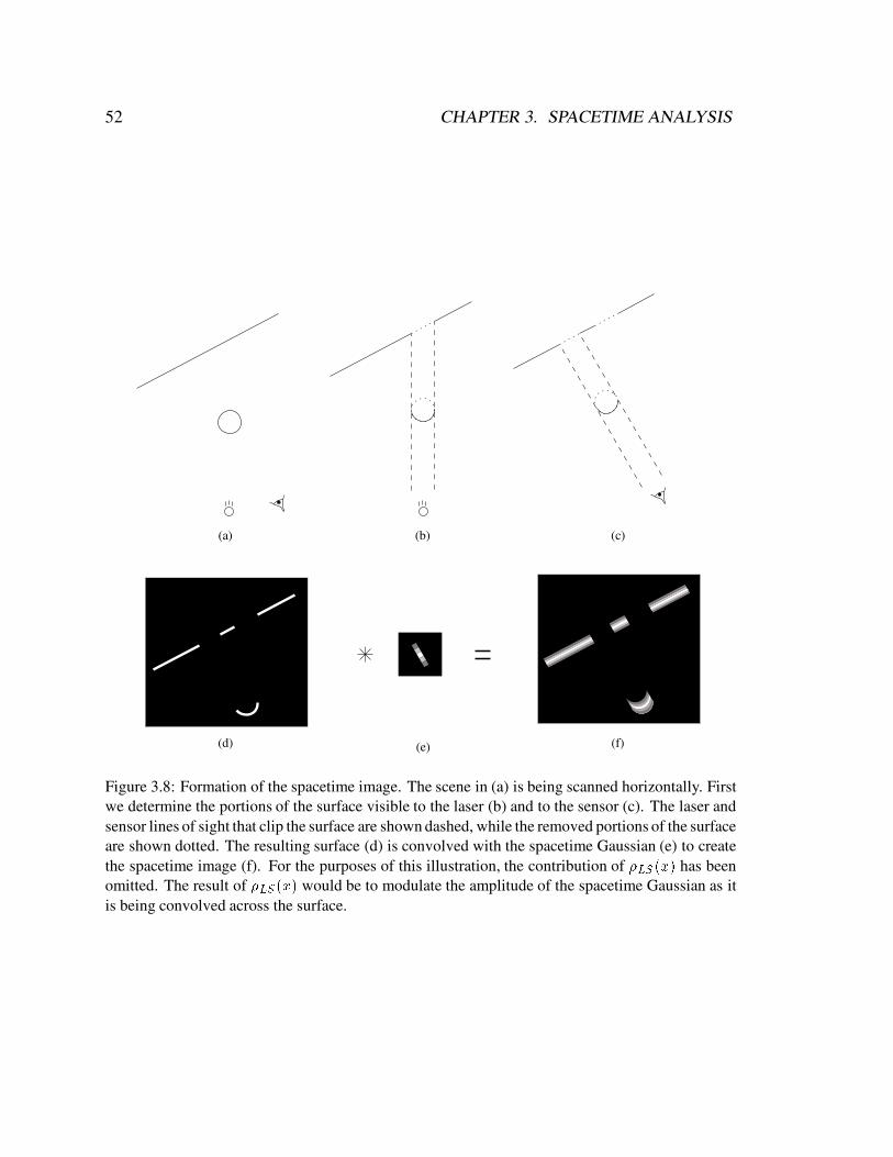
52 CHAPTER 3. SPACETIME ANALYSIS
(c)
(d) (e) (f)
(b)(a)
Figure 3.8: Formation of the spacetime image. The scene in (a) is being scanned horizontally. Firstwe determine the portions of the surface visible to the laser (b) and to the sensor (c). The laser andsensor lines of sight that clip the surface are shown dashed, while the removed portions of the surfaceare shown dotted. The resulting surface (d) is convolved with the spacetime Gaussian (e) to createthe spacetime image (f). For the purposes of this illustration, the contribution of �LS (x) has beenomitted. The result of �LS (x) would be to modulate the amplitude of the spacetime Gaussian as itis being convolved across the surface.

3.5. A SIGNAL PROCESSING PERSPECTIVE 53
3.5.2 Filtering, noise, sampling, and reconstruction
The function ES(x; z) represents the ideal spacetime image, and if we could acquire it per-
fectly, then we would be able to compute the exact shape of the object. In the real world,
however, this image is filtered, corrupted by noise, sampled, and ultimately reconstructed
before being analyzed for shape extraction.
The filtering can be decomposed into two components: spatial and temporal. Spatial
blurring occurs at the sensor due to the imaging optics and the fact that each sensor cell
has a finite area over which it gathers photons and accumulates a charge. We call this filter
hpix (z), because it spans sensor pixels. The other filtering component operates temporally;
as the object moves relative to the scanner, the sensor captures photons over a fixed interval
of time before sampling the result and starting over. The motion is effectively blurred during
this interval. We call this temporal filter hframe(x), where “frame” refers to the time interval
and x is the representative of the time component (remember, x = vt).
Several noise sources also affect the spacetime image. As described in the previous sec-
tion, coherent illumination leads to speckle noise that corrupts the spacetime Gaussian. In
addition, the sensor will have some inherent noisiness caused by a variety of factors (see,
e.g., [Janesick et al. 1987]). Finally, during the sampling step, the pixel values will be quan-
tized for representation in the computer, introducing quantization noise. We will represent
all of these noise sources with one function, �().
Putting the filtering and noise sources together, we arrive at an expression for the space-
time image prior to sampling and reconstruction:
E�ltS (x; z) = �[ES(x; z) � hpix (z) � hframe(x)] (3.15)
This image is then sampled according to the spatial resolution of the sensor and the frame
rate. We represent this sampling process as an impulse train, i( x
�x; z
�z), where �z is the sensor
pixel separation projected along the laser sheet and �x is the distance the object moves rel-
ative to the scanner between frames. Once we have the sampled, filtered spacetime image,
we can employ a reconstruction filter, hrec(x; z), to obtain an approximation to the original
continuous image. This final image is then:

54 CHAPTER 3. SPACETIME ANALYSIS
~ES(x; z) =�E�ltS (x; z) � i
�x
�x;z
�z
��� hrec(x; z) (3.16)
One of the first observations that arises from these equations is the fact that the recon-
structed spacetime image is a continuous function. Thus, this reconstruction yields a (piece-
wise) continuous surface, rather than a set of range samples. In the next chapter, we exploit
this observation to extract as much range data as possible.
3.5.3 The spacetime spectrum
Taking the Fourier transforms of Equations 3.11 - 3.16 will provide several insights. For
simplicity, we omit the influence of noise and arrive at the following relations:
F(ES) = F (sx; sz)HST (sx; sz) (3.17)
F(E�ltS ) = F(ES)Hpix (sz)Hframe (sx)] (3.18)
F( ~ES) = [F(E�ltS ) � �x�zi(�xsx; �zsz)]Hrec(sx; sz) (3.19)
where F() is the Fourier transform operator, sx and sz are the spatial frequencies in x and
z, and F , HST , Hpix , Hframe , and Hrec are the Fourier transforms of f , hST , hpix , hframe ,
and hrec , respectively. Figure 3.9 shows the steps in creating, filtering, and sampling the
spacetime image.
Several observations arise from thinking about the Fourier spectrum of the spacetime
image. The least surprising is the fact that higher sampling rates permit (and are usually
accompanied by) wider Hpix and Hframe filters, allowing for the acquisition of more of the
spacetime spectrum, i.e., higher frequencies. In other words, a higher sampling rate leads
to more captured detail.

3.5. A SIGNAL PROCESSING PERSPECTIVE 55
F(ES)
F(E�ltS
)HpixHframe
(a) (b) (c)
(d) (e)
F
sx
sz
HST
�
(f)
1=�x
1=�z
sz sz
sz
szsz
sx
sx
sx sx
sx
1=w0
Figure 3.9: The spacetime spectrum: a visualizationfor Equations3.17 - 3.19. The Fourier transformof the shape function (a) is multiplied by the spectrum of the spacetime Gaussian (b) to give thespectrum of the ideal spacetime image (c). Before sampling, this spectrum is multiplied by the pixeland frame filters (shown as idealized low-pass filters in (d)) to give the filtered spacetime spectrumwithout noise (e). The sampling process creates replicas of this filtered spectrum (f) spaced 1=�x and1=�z apart in sx and sz respectively. The reconstruction step entails extracting the central replica ofthe spectrum after multiplying by Hrec (not shown).

56 CHAPTER 3. SPACETIME ANALYSIS
3.5.4 Widening the laser sheet
The Fourier spectrum also tells us that the spacetime Gaussian acts like a bandlimiting filter
that runs along the sensor lines of sight, as indicated in Figure 3.9c. Note that this “filter”
does not remove detail, as in the case of the pixel and frame filters. The resulting spacetime
image is still ideal and contains all the information required to extract the original surface
geometry precisely. Thus, by narrowing the spectrum of the spacetime Gaussian, we can re-
strict the spectrum of the spacetime image without loss of detail. The surprising conclusion:
widening the illuminant can improve results.
Consider scanning a line (a plane in 3D), as depicted in Figure 3.10. The Fourier trans-
form of this line is another line, perpendicular to the first. After superimposing the spectrum
of the spacetime Gaussian, we arrive at the ideal spacetime spectrum, which is basically a
line segment in the Fourier plane. The length of this line segment corresponds to the max-
imum frequency content of the spectrum and thus determines the sampling rate needed to
acquire the surface. The parameters that determine the length of the Fourier line segment are
the orientation of the original line, the width of the laser sheet, and the triangulation angle.
For a fixed laser width and triangulation angle, the spectral line segment grows in length
as the line is rotated to be at more of a grazing angle to the sensor. At a critical angle, the
pixel and frame filters begin to clip the spectral line segment and degrade the quality of the
reconstruction; worse, if the filters are not ideal (and, generally, they are not), aliasing will
occur. By widening the laser sheet, however, this critical angle can be extended closer to
the triangulation angle.
This notion of widening the laser sheet runs counter to the intuition that a narrower il-
luminant gives better localization of the point on the surface being acquired. This intuition,
however, stems from thinking of triangulation in the traditional context. In the spacetime
context, the wider beam does not degrade resolution by “blurring” neighboring points to-
gether. It is interesting to note that while the accuracy of the traditional method improves
with a narrower laser sheet in principle, in practice the laser must have a minimum thickness
to avoid range errors due to aliasing. For a surface of fixed orientation, narrowing the laser
sheet also narrows the imaged Gaussian on the sensor, until eventually it is narrower than
a pixel cell. At this point, the accuracy is limited by the width of a pixel projected onto the

3.5. A SIGNAL PROCESSING PERSPECTIVE 57
sx
sz
sx
sz
F
F(ES)
(b)
(c)
x
z
(d)
�
�
f
�
(a)
� �
�
Figure 3.10: Spacetime spectrum for a line. (a) A line at angle � to the laser is scanned. (b) Thefunction to be convolved with the spacetime Gaussian is a delta function line. (c) Its Fourier trans-form is another delta function line oriented perpendicular to the original. (d) After “filtering” withthe spacetime Gaussian, the spacetime spectrum is essentially a line segment in the Fourier plane.
laser sheet, not the width of the laser.
In practice, the laser sheet cannot be widened arbitrarily. The primary limitation is the
depth of field of the sensor. As the laser is widened, the sensor must record more of the
object that is out of the plane of focus. The out of focus points will be blurred, and the
improvement from the laser sheet will be countered. One solution might be to use a brighter
beam and then stop down the sensor’s aperture to increase the depth of field. However, for
coherent illumination, the narrowed aperture leads to increased speckle noise which can also
defeat the improved accuracy. Even incoherent imaging systems will approach a diffraction
limit as the aperture is narrowed. In addition, as the laser sheet widens, then the effects of
using a sensor with perspective projection become more prevalent, as noted in Section 3.3.
Further, speckle analysis indicates that widening the laser sheet increases the influence due

58 CHAPTER 3. SPACETIME ANALYSIS
to speckle noise. Nevertheless, by balancing these trade-offs, it should be possible to realize
a system with improved accuracy. This remains an area for future work.
3.5.5 Improving resolution
Fourier analysis of the spacetime image also reminds us of the importance of using good
bandlimiting filters, Hpix and Hframe , to avoid aliasing artifacts. However, we do not have
much control over these filters. The pixel filter is essentially the convolution of the blur-
ring due to finite pixel cell size with any optical blurring that may occur. When the laser
sheet is in focus, then the sensor’s pixel response is the primary filter, which in turn is set
by the design of the sensor. The frame filter is essentially a rectangle function in x with
width proportional to the exposure time. In addition, sensors generally have a time interval
when they stop capturing light while shifting out the recorded signals. The spectral band-
width of the temporal filter is thus wider than the distance between samples. In both the
spatial and temporal cases, some aliasing artifacts are bound to occur. This aliasing gen-
erally leads to reduction in image quality; however, it also means that multiple spacetime
images may be combined to improve the accuracy of the range data. Techniques such as the
one described in [Irani & Peleg 1991] could be used to combine these spacetime images. In
order for such an approach to work, a sequence of spacetime images must be acquired after
translating the object (or scanner) between scans. Rotating the object (or scanner) between
scans generates an entirely new spacetime image that may not be combined with prior ac-
quisitions. Increased resolution through combination of multiple spacetime images remains
an area for future work.

3.5. A SIGNAL PROCESSING PERSPECTIVE 59

Chapter 4
Spacetime analysis: implementation and
results
The previous chapter provides a theoretical foundation for accurate optical triangulation
through spacetime analysis. In this chapter, we demonstrate that the method can be adapted
to work with an existing commercial laser triangulation scanner (Section 4.1). We develop
an efficient algorithm for performing the spacetime analysis and show how increased res-
olution can be obtained by interpolating the imaged light reflections (Section 4.2). Finally,
we show the results of applying the spacetime analysis to some real objects (Section 4.3).
4.1 Hardware
We have implemented the spacetime analysis presented in the previous chapter using a com-
mercial laser triangulation scanner and a real-time digital video recorder. The optical trian-
gulation system we use is a Cyberware MS 3030 platform scanner (shown in Figure 1.5).
This scanner collects range data by casting a laser stripe onto the object and by observing
reflections with a CCD camera positioned at an angle of 30o with respect to the plane of the
laser. The platform can either translate or rotate an object through the field of view of the
triangulation optics. Figure 1.2b illustrates the principle of operation. The laser width (the
distance between the beam center and the e�2 point) varies from 0.8 mm to 1.0 mm over the
field of view which is approximately 30 cm in depth and 30 cm in height. Each CCD pixel
60

4.1. HARDWARE 61
Transfer to hostand RLE compress
Cosmo JPEG decompressand RLE recompress
Cosmo JPEG compress(real-time, high quality)
Cyberwarevideo camera
Abekas digitizer
Abekas video disk
Spacetime analysis
Range image
Figure 4.1: From range video to range image. To perform the spacetime analysis, we digitize the Cy-berware video with an Abekas digitizer. We can then either store the digitized video to disk and copyit to the host computer, or perform a real-time JPEG compression and fast decompression throughan SGI Cosmo board. The JPEG compression approach has proven to be more time efficient, but theresults in this chapter were originally obtained with the video disk option. In either case, the framesare run-length encoded and then converted to a range image through the spacetime analysis.

62 CHAPTER 4. SPACETIME ANALYSIS: IMPLEMENTATION AND RESULTS
images a portion of the laser plane about 0.5 mm square. Although the Cyberware scanner
performs a form of peak detection in real time, we require the actual video frames of the
camera for our analysis. Figure 4.1 illustrates the possible routes for processing the range
video. We can digitize these frames with an Abekas A20 video digitizer, which can acquire
486 by 720 pixel frames at 30 Hz. The captured frames have approximately the same res-
olution as the Cyberware CCD camera, though the scanlines are first converted to analog
video before being resampled and digitized. The digitized frames can then be stored in real
time with an Abekas A60 digital video disk. Alternatively, we can run the digitized signal
through a commercially available JPEG compression board. Because each frame is an im-
age of the narrow laser sheet intersecting the surface, it is mostly blank. As a result, we
can JPEG compress the frame with a high quality factor, but still obtain high compression.
The JPEG compression efficiently encodes the blocks of empty space without sacrificing the
quality of the imaged light reflections. The key advantage of this approach is that the range
video compresses well enough to be stored on the host computer’s main memory, as op-
posed to a video disk which limits the speed of recovery of the recorded frames. The results
in this chapter were obtained with the Abekas digital video disk, but the results described
in Chapter 8 are based on range data acquired with the help of JPEG compression.
4.2 The spacetime algorithm
Using the principles of the previous chapter, we can devise a procedure for extracting range
data from spacetime images:
1. Perform the range scan and capture the spacetime images.
2. Rotate the spacetime images by �.
3. Find the statistics of the Gaussians in the rotated coordinates.
4. Rotate the means back to the original coordinates.
Figure 4.2 illustrates this new method graphically. In order to implement step 1 of this
algorithm, we require a sequence of CCD images. Most commercial optical triangulation

4.2. THE SPACETIME ALGORITHM 63
(b) (c) (d) (e)(a)
z
x
z
x
z
x
x
z
x
z
Figure 4.2: Method for optical triangulationrange imaging with spacetime analysis. (a) The originalgeometry. (b) The resulting spacetime image when scanning with the illuminant in the+z direction.(c) Rotation of the spacetime image followed by evaluation of Gaussian statistics. (d) The means ofthe Gaussians. (e) Rotation back to world coordinates.
systems discard each CCD image after using it (e.g. to compute a stripe of the range map).
As described in the previous section, we have assembled the necessary hardware to record
the CCD frames. In the previous chapter, we discussed a one dimensional sensor scenario
and indicated that perspective imaging could be treated as locally orthographic. For a two
dimensional sensor, we can imagine the horizontal scanlines as separate one dimensional
sensors with varying vertical (y) offsets. Each scanline generates a spacetime image, and
by stacking the spacetime images one atop another, we define a spacetime volume. Compli-
cations arise when we have perspective projection in the vertical direction, as the image of a
point sweeping through the Gaussian illuminant can cross scanlines (i.e., a point is not con-
strained to lie in a single spacetime image plane). We have not yet implemented the general
spacetime ranging method that accounts for this effect, so we restrict most of our analysis
to the spacetime volume near the vertical centerline of the CCD where range points will not
cross scanlines while passing through the illuminant (i.e., we can visualize the spacetime
volume as a stack of spacetime images). Nevertheless, toward the end of this chapter, we
demonstrate some results for larger objects that show improvement even though they are
not restricted to the center of the field of view in the vertical direction. This improvement is
probably due to the fact that even at the extreme positions of the field of view a point does
not traverse more than half a scanline while passing through the illuminant.
In step 2, we rotate the spacetime images so that Gaussians are vertically aligned. In a
practical system with different sampling rates in x and z, the correct rotation angle can be
computed as:

64 CHAPTER 4. SPACETIME ANALYSIS: IMPLEMENTATION AND RESULTS
tan �ST =�z�x
tan � (4.1)
where �ST is the new rotation angle, �x and �z are the sample spacings in x and z respec-
tively, and � is the triangulation angle. In order to determine the rotation angle, �ST , for a
given scanning rate and region of the field of view of our Cyberware scanner, we first de-
termined the local triangulation angle and the sample spacings in depth, z, and lateral posi-
tion, x. Equation 4.1 then yields the desired angle. When performing the rotation, we avoid
aliasing artifacts which would lead to range errors by employing high-quality filters. For
this purpose, we use a bicubic interpolant.
After performing the rotation of each spacetime image, we compute the statistics of the
Gaussians along each rotated spacetime image raster1. Our method of choice for computing
these statistics is a least squares fit of a parabola to the log of the data; i.e, given a Gaussian
of the form:
G(x) = a exp
"�2(x� b)2
w2
#
where a is the amplitude and b is the desired center, we can take the log of the Gaussian:
log[G(x)] = log[a]� 2(x� b)2
w2=�� 2
w2
�x2 +
4b
w2
!x+
log[a]� 2b2
w2
!
and fit a parabola to the result. The linear coefficient contains the center, b.
We have also experimented with fitting the data directly to Gaussians using the
Levenberg-Marquardt non-linear least squares algorithm [Press et al. 1986], but the results
have been substantially the same as the log-parabola fits.
The Gaussian statistics consist of a mean, which corresponds to a range point, as well as
a width and a peak amplitude, both of which indicate the reliability of the data. Widths that
are far from the expected width and peak amplitudes near the noise floor of the sensor im-
ply unreliable data which may be down-weighted or discarded during later processing (e.g.,
1Actually, we do not expect to find perfect Gaussians on the rotated image rasters. The filtering and sam-pling processes described in Section 3.5 alter the ideal spacetime image. Nevertheless, fitting Gaussians is areasonable approximation that has yielded excellent results in practice

4.2. THE SPACETIME ALGORITHM 65
Type: varyingLength: 11Data: 4, 18, 65, ...
Type: zeroesLength: 17
Type: zeroesLength: 10
Figure 4.3: Run-length encoded spacetime scanline. Each scanline is composed of runs of zeroesand runs of varying intensity data.
when combining multiple range meshes). For the purposes of this thesis, we discard unre-
liable data and rely on future scans to fill in reliable data used in the surface reconstruction
process.
Finally, in step 4, we rotate the range points back into the global coordinate system.
4.2.1 Fast rotation of the spacetime image
In order to process the spacetime images, we first compress the frames into a run length en-
coded (RLE) representation as shown in Figure 4.3. The time evolution of a single scanline
is thus a run length encoded spacetime image which we must rotate in order to extract range
data. The naive approach to rotating each image would be to expand it into uncompressed
form, and then visit the pixels of the target image while walking through the rotated source
slice, i.e., while “gathering” data from the source slice. Alternatively, we can process the
source image’s runs, and only “send” data to the source image in the regions of runs with
varying data [Lacroute 1995]. Figure 4.4 illustrates this principle.
Note that when performing the traditional gather approach, we step through the target
image and resample the source image using a reconstruction filter. As a result, a neighbor-
hood of source pixels will influence the value of each target pixel, as shown in Figure 4.5c.
We can also look at this in another way: each source pixel will influence a neighborhood of
target pixels. Thus, when performing the send operation, each pixel adds weighted copies
of itself to a neighborhood of pixels in the target image. This send operation is illustrated
in Figure 4.5d.
The RLE send method we have described so far will significantly reduce the computa-
tional expense, because it visits only the interesting pixels in the source image. Neverthe-
less, it still creates an uncompressed target image whose pixels must all be visited in the

66 CHAPTER 4. SPACETIME ANALYSIS: IMPLEMENTATION AND RESULTS
Rotated image
Spacetime image
Send
Gather
Figure 4.4: Fast RLE rotation. The naive approach to rotating an image would be to expand theRLE source image, and then traverse all of the pixels of the target image while “gathering” data from(resampling) the source image. A much more efficient approach is to traverse the RLE structure inthe source image and “send” only non-zero data to the target image.
A
B
(a) (b)
(c) (d)
Source
Target
AB
Figure 4.5: Reconstruction: send vs. gather. (a) The target image is rotated with respect to the sourceimage. (b) We can find the values at the target pixels by interpolating among the source pixels. (c)“Gather” interpolation for a single target image pixel, A. (d) “Send” interpolation for a single sourcepixel. The example in this figure illustrates the case for a bilinear filter with a 2x2 support; extensionto filters with larger supports is straightforward.

4.2. THE SPACETIME ALGORITHM 67
next step of the spacetime algorithm. Ideally, we would like to create an RLE target image
directly. We can achieve this goal with the following procedure:
1. Allocate space for each scanline in the target image.
2. Stream through each source scanline, ignoring runs of zeroes. When sending varying
data:
� If the data being sent is not within the current target run being constructed:
– Mark the current target run as finished.
– Declare a run of zeroes between the finished run and the new target position.
– Start a new run of varying pixels.
� Else,
– Deposit the pixel value into the existing run, increasing its length as needed.
3. Mark the last run on each scanline as being a run of zeroes.
Figure 4.6 shows a scanline as it is being constructed.
This RLE rotation algorithm delivers a dramatic performance improvement. If we con-
sider a spacetime volume of n voxels on a side, then the brute force rotation would execute
in time proportional to the size of the volume, i.e., O(n3). On the other hand, the fast algo-
rithm described here requires time proportional to the part of the volume with non-zero data.
The sensor samples the surface onto a grid of size roughly n x n, which is then “blurred”
into the spacetime volume by the spacetime impulse response (Equation 3.11). The width
of this impulse response function is constant, so the overall size of the spacetime surface
embedded in the volume is O(n2). Thus, the fast rotation algorithm runs in O(n2) time,
substantially faster then the brute force method. In practice, we observe a typical speed-up
of 50:1 over the brute force approach.

68 CHAPTER 4. SPACETIME ANALYSIS: IMPLEMENTATION AND RESULTS
A
B
C
D
(a)
(b)
Rotation
T = ?L = ?
T = ZL = 20
T = VL = 1
T = VL = 7
T = VL = 7
T = ZL = 6
T = ZL = 6
T = VL = 1
T = VL = 7
T = ZL = 15
T = ZL = 20
T = ZL = 20
Figure 4.6: Building a rotated RLE scanline. (a) The source image is traversed in scanline order(dotted white lines) from top to bottom (solid black arrow to the left), and the non-zero values aredeposited in the target image. (b) The scanline indicated by the solid white arrow in the target imageis constructed in steps. “T” is the data type, and “L” is the run length. In A, The scanline is initializedto have no data or length. In B, when the first source scanline intersects the target scanline, the firstrun is declared to be zeroes (T = Zero or “Z”) and its length is computed. In addition, a varying run(T = Varying or “V”) is begun. As successive source scanlines intersect the target scanline, morevarying data is added to the current run, which grows as needed. At C, more varying data is laiddown, but it is offset from the first varying run. Thus, a new run of zeroes is declared with its length,and a new varying run is begun. Eventually, the source scanline sweep finishes, and the remainderof the scanline is declared to be zeroes, as shown in D.

4.2. THE SPACETIME ALGORITHM 69
(a) (b)
z
x
z
x
Extractedrange points
Spacetimeimage
Figure 4.7: Interpolation of spacetime image data. (a) Extraction of range data from a spacetimeimage followed by linear interpolation of the range points. (b) Same as (a) but more interpolation inthe spacetime image rather than the among the range points.
4.2.2 Interpolating the spacetime volume
Traditionally, researchers have extracted range data at sampling rates corresponding to one
range point per sensor scanline per unit time. Interpolation of shape between range points
has consisted of fitting primitives (e.g., linear interpolants like triangles) to the range points.
Instead, we can regard the spacetime volume as the primary source of information we have
about an object. After performing a scan, we have a sampled representation of the spacetime
volume, which we can then reconstruct to generate a continuous function. In the previous
chapter, we described this reconstruction for a spacetime image; for the spacetime volume,
we have added a vertical dimension, but the principle remains the same. This reconstructed
function then acts as our range “oracle,” which we can query for range data at a resampling
rate of our choosing. Figure 4.7 illustrates this idea for a single spacetime image. In practice,
we can magnify the sampled spacetime volume prior to applying the range imaging steps
described above. The result is a range grid with a higher sampling density directly derived
from the imaged light reflections.

70 CHAPTER 4. SPACETIME ANALYSIS: IMPLEMENTATION AND RESULTS
Scanline mean� Spacetime Gaussian
|1
|3
|5
|7
|9
|11
|13
|0.0
|0.2
|0.4
|0.6
|0.8
Reflectance Ratio
Err
or (
mm
)
�������� �
� �
(a) (b)
Figure 4.8: Measured error due to reflectance step. (a) Printed cards with reflectance discontinuitieswere carefully taped to a machined planar surface. The black dots were used to distinguish the tapedboundary from the target surface. (b) A plot of range errors shows that the spacetime method yieldsa 60-80% reduction in range error for steps varying from 1:1 to 12:1.
4.3 Results
We have performed a variety of tests to evaluate the performance of traditional triangulation
and spacetime analysis. These tests include experiments with reflectance variations, simple
shape variations, errors due to speckle, and scanning complex objects.
4.3.1 Reflectance correction
To evaluate the tolerance of the spacetime method to changes in reflectance, we performed
two experiments, one quantitative and the other qualitative. For the first experiment, we pro-
duced reflectance steps by printing alternating white and gray stripes with a color printer. By
varying the reflectances of the solid gray stripes, we obtained reflectance ratios (white:gray)
of about 1:1 to 10:1. We scanned them at an angle of 30o (roughly facing the sensor) and ex-
tracted range data using both the traditional method and the spacetime method. To measure
deviations from planarity, we first computed the parameters of the plane by deleting those
range points lying in the neighborhood of the reflectance discontinuity. This step avoids per-
mitting erroneous data to influence the estimated orientation of the plane. When comput-
ing range errors, we used all range data, including points near the reflectance discontinuity.

4.3. RESULTS 71
(a)
(b) (c)
Figure 4.9: Reflectance card. (a) Photograph of a planar card with the word “Reflectance” printedon it. (b) and (c) Shaded renderings of the range data generated by traditional mean analysis andspacetime analysis, respectively. With traditional mean analysis, the planar card appears embossedwith the lettering, indicating a confusion between reflectance and shape. The spacetime analysisyields a nearly planar surface, showing a disambiguation of reflectance and shape.
Figure 4.8 shows a plot of maximum deviations from planarity. The spacetime method has
clearly improved over the old method. The reduction in range errors varies from 65% for a
reflectance change of 2:1 up to 85% for a reflectance change of 12:1.
For qualitative comparison, we produced a planar sheet with the word “Reflectance”
printed on it. Figure 4.9 shows the results. The old method yields a surface with the charac-
ters well-embossed into the geometry, whereas the spacetime method yields a much more
planar surface indicating successful decoupling of geometry and reflectance.
4.3.2 Shape correction
We conducted several experiments to evaluate the effects of shape variation on range ac-
quisition. In the first experiment, we generated corners of varying angles by abutting sharp
edges of machined aluminum wedges which were painted white. Figure 4.10 shows the
range errors that result for traditional and spacetime methods. Again, we see an increase in
accuracy, though not as great as in the reflectance case.
We also scanned two 4 mm strips of paper at an angle of 30o (roughly facing the sensor)
to examine the effects of depth discontinuities. Figure 4.11b shows the “edge curl” observed
with the old method, while the spacetime method in Figure 4.11c shows a significant reduc-
tion of this artifact under spacetime analysis. We have found that the spacetime method re-
duces the length of the edge curl from an average of 1.1 mm to an average of approximately
0.35 mm.

72 CHAPTER 4. SPACETIME ANALYSIS: IMPLEMENTATION AND RESULTS
Scanline mean� Spacetime Gaussian
|100
|120
|140
|160
|0.0
|0.1
|0.2
|0.3
|0.4
|0.5
Corner Angle (degrees)
Dis
tanc
e to
cor
ner
(mm
)
�
�
�
�
(a)
(b)
Figure 4.10: Measured error due to corner. (a) Two machined wedges with razor sharp corners wereplaced at varying angles to each other to study the effect of corner angle on range accuracy. (b) Aplot of range errors shows that the spacetime method yields a 35-50% reduction in range error forcorners of angles varying from 110o to 150o.
(a) (b) (c)
Figure 4.11: Depth discontinuities and edge curl. (a) Photograph of two strips of paper. (b) and (c)Shaded renderings of the range data generated by traditional mean analysis and spacetime analysis,respectively. With traditional mean analysis, the edges of the strips exhibit large edge curl artifacts(1.1 mm between the hash marks in (b)). The curl is nearly eliminated when using the spacetimeanalysis.
Finally, we impressed the word “SHAPE” onto a plastic ribbon using a commonly avail-
able label maker. In Figure 4.9, we wanted the word “Reflectance” to disappear because it
represented changes in reflectance rather than in geometry. In Figure 4.12, we want the word
“SHAPE” to stay because it represents real geometry. Furthermore, we wish to resolve it as
highly as possible. Figure 4.12 shows the result. Using traditional mean analysis, the word
is barely visible. Using spacetime analysis, the word becomes legible.

4.3. RESULTS 73
(a)
(b) (c)
Figure 4.12: Shape ribbon. (a) Photograph of a surface with raised lettering (letters are approx. 0.3mm high). (b) and (c) Shaded renderings of the range data generated by traditional mean analysisand spacetime analysis, respectively. Using mean pulse analysis, the lettering is hardly discernible,while the spacetime analysis yields a legible copy of the original shape.
4.3.3 Speckle
To evaluate the influence of laser speckle, we scanned planar surfaces of varying roughness
under coherent and incoherent light. First, we verified the existence of the laser speckle.
Recording the light reflections from the surfaces under incoherent (single filament, non-
diffuse) illumination showed negligible variation (< 5%) in image intensity, while the im-
ages of laser reflections showed significant variations (> 20%) in peak intensity. These
facts, coupled with the observation that surfaces with roughness finer than the resolution
of the pixels yielded variations at a scale larger than a pixel, lead us to believe that we are
observing laser speckle.
Next, we performed range scans on the planar surfaces and generated range points using
the traditional and spacetime methods. After fitting planes to range points, we found that
both methods resulted in range errors with a standard deviation of about 0.06 mm and a
distribution that is very nearly Gaussian (see Figure 4.13). As expected, both traditional
and spacetime triangulation are susceptible to errors due to laser speckle. In Section 2.2.4,
we computed the range error for a perfectly rough surface to be 0.25 mm. Since the surface
being measured is unlikely to be perfectly rough, it is not surprising that the measured error
is less.
4.3.4 Complex objects
To show how the spacetime analysis performs with more complex objects occupying a larger
portion of the field of view, we scanned two models. Figure 4.14 shows the results for a
model tractor. Figure 4.14b is a rendering of the data generated by the Cyberware scanner

74 CHAPTER 4. SPACETIME ANALYSIS: IMPLEMENTATION AND RESULTS
−0.15 −0.1 −0.05 0 0.05 0.1 0.150
20
40
60
80
100
120
Num
ber
of p
oint
s
Distance from surface (mm)
Bars = range data
Line = Gaussian fit
Figure 4.13: Distribution of range errors over a planar target. We extracted the range data usingspacetime analysis and fit a plane through the resulting data. The bar graph represents a histogramof distances from the planar fit, while the curve corresponds to a Gaussian approximation to the his-togram.
hardware and is particularly noisy. This added noisiness results from the method of pulse
analysis performed by the hardware, a method similar to peak detection. Peak detection is
especially susceptible to speckle noise, because it extracts a range point based on a single
value or small neighborhood of values on a noisy curve. Mean analysis tends to average out
the speckle noise, resulting in smoother range data as shown in Figure 4.14c. Figure 4.14d
shows our spacetime results and Figure 4.14e shows the spacetime results with 3X interpo-
lation and resampling of the spacetime volume as described in Section 4.2. Note the sharper
definition of features on the body of the tractor.
Figure 4.15 shows the result for a model of an alien creature. As with the tractor image,
the Cyberware output is noisier than the traditional mean analysis results. Note, however,
that the traditional mean analysis appears to smooth the geometric detail more than the Cy-
berware method. Both the Cyberware and the mean analysis suffer from edge curl. By con-
trast, the spacetime method reduces edge curl, exhibits less noise, and attains comparable
or greater detail than either of the other methods.

4.3. RESULTS 75
(a)
(b) (c)
(d) (e)
Figure 4.14: Model tractor. (a) Photograph of original model and shaded renderings of range datagenerated by (b) the Cyberware scanner hardware, (c) mean pulse analysis, (d) our spacetime anal-ysis, and (e) the spacetime analysis with 3X interpolation of the spacetime volume before fitting theGaussians. Below each of the renderings is a blow-up of one section of the tractor body (indicated byrectangle on rendering) with a plot of one row of pixel intensities. Because of the scanner hardware’speak detection method, it is the most susceptible to speckle noise as is evident in the rendering and inthe “bumpy” intensity plot. Mean analysis yields a decrease in noise and spacetime analysis yieldseven less noise and more detail. The 3X interpolated spacetime analysis reveals the most detail ofall.
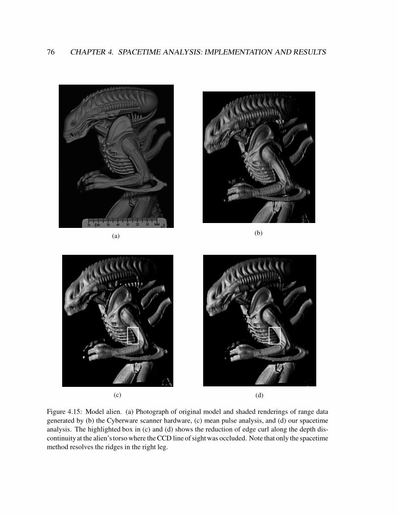
76 CHAPTER 4. SPACETIME ANALYSIS: IMPLEMENTATION AND RESULTS
(a) (b)
(c) (d)
Figure 4.15: Model alien. (a) Photograph of original model and shaded renderings of range datagenerated by (b) the Cyberware scanner hardware, (c) mean pulse analysis, and (d) our spacetimeanalysis. The highlighted box in (c) and (d) shows the reduction of edge curl along the depth dis-continuityat the alien’s torso where the CCD line of sight was occluded. Note that only the spacetimemethod resolves the ridges in the right leg.

4.3. RESULTS 77
4.3.5 Remaining sources of error
The results we presented in this section clearly show that the spacetime analysis yields more
accurate range data, but the results are imperfect due to system limitations. These limita-
tions include:
� CCD noise
� Finite sensor resolution
� Optical blurring and electronic filtering
� Quantization errors
� Calibration errors
� Surface-surface inter-reflections
In addition, we observed some electronic artifacts in our Cyberware scanner that influ-
enced our results. We expect, however, that any measures taken to reduce the effects of
the limiting factors described above will lead to higher accuracy. By contrast, if one uses
traditional methods of range extraction, then increasing sensor resolution and reducing the
effects of filtering alone will not significantly increase tolerance to reflectance and shape
changes when applying the traditional methods of range extraction.

Chapter 5
Surface estimation from range images
The second part of this thesis is concerned with building computer models from range im-
ages such as might be generated using the method described in the first part of the thesis.
As stated in Chapter 1, the problem of reconstructing a surface from range images can
be stated as follows:
Given a set of p aligned, noisy range images, f1; � � � ; fp, find the 2D manifold
that most closely approximates the points contained in the range images.
where each function, fi is a sampling of the actual surface f , and each sample, fi(j; k) is
the observed distance to the surface as seen along the line of sight indexed by (j; k). The
problem of finding this manifold hinges on defining how well any manifold approximates
the range images, and then solving for the “best” manifold. In this chapter, we begin with a
discussion of prior work in reconstructing surfaces from range data. Next, we describe range
imaging in more detail and then construct a probabilistic model relating possible manifolds
to range image samples. In Section 5.4, we define the best surface as the Maximum Like-
lihood surface, and we define the integral that this surface must minimize. In Section 5.5,
we show how to bring the integral under a unified domain using a vector field analogy for
range image sampling. In Section 5.6, we derive some results from the calculus of varia-
tions needed for the solution of this minimization problem. Finally, in Section 5.7, we solve
the minimization equation for surface reconstruction from range images. As a special case,
78

5.1. PRIOR WORK IN SURFACE RECONSTRUCTION FROM RANGE DATA 79
we relate the least squares minimization (corresponding to Gaussian statistics) to the search
for a zero crossing of weighted sums of signed distance functions.
5.1 Prior work in surface reconstruction from range data
Surface reconstruction from dense range data has been an active area of research for several
decades. The strategies have proceeded along two basic directions: reconstruction from un-
organized points, and reconstruction that preserves the underlying structure of the acquired
data. These two strategies can be further subdivided according to whether they operate by
reconstructing polygonal surfaces or by reconstructing an implicit function.
5.1.1 Unorganized points: polygonal methods
A major advantage of the unorganized points algorithms is the fact that they do not make any
prior assumptions about connectivity of points. In the absence of range images or contours
to provide connectivity cues, these algorithms are the only recourse. Among the polygonal
surface approaches, Boissonnat [1984] describes a method for Delaunay triangulation of a
set of points in 3-space. Edelsbrunner & Mucke [1992] generalize the notion of a convex
hull to create surfaces called alpha-shapes.
5.1.2 Unorganized points: implicit methods
Examples of implicit surface reconstruction include the method of Hoppe et al. [1992] for
generating a signed distance function followed by an isosurface extraction. More recently,
Bajaj et al. [1995] used alpha-shapes to construct a signed distance function to which they
fit implicit polynomials.
Although unorganized points algorithms are widely applicable, they discard useful in-
formation such as surface normal and reliability estimates. As a result, these algorithms are
well-behaved in smooth regions of surfaces, but they are not always robust in regions of
high curvature and in the presence of systematic range distortions and outliers.

80 CHAPTER 5. SURFACE ESTIMATION FROM RANGE IMAGES
5.1.3 Structured data: polygonal methods
Among the structured data algorithms, several polygonal approaches have been proposed.
Soucy & Laurendeau [1992] describe a method using Venn diagrams to identify overlapping
data regions, followed by re-parameterizationand merging of regions. Turk & Levoy [1994]
employ an incremental algorithm that updates a reconstruction by eroding redundant geom-
etry, followed by zippering along the remaining boundaries, and finally a “consensus” step
that reintroduces the original geometry to establish final vertex positions. Rutishauser et al.
[1994] use errors along the sensor’s lines of sight to establish consensus surface positions
followed by a re-tessellation that incorporates redundant data. These algorithms typically
perform better than unorganized point algorithms, but they can still fail catastrophically in
areas of high curvature.
5.1.4 Structured data: implicit methods
Several algorithms have been proposed for integrating structured data to generate implicit
functions. These algorithms can be classified as to whether voxels are assigned one of two
(or three) states or are samples of a continuous function.
Discrete-state voxels
Among the discrete-state volumetric algorithms, Connolly [1984] casts rays from a range
image accessed as a quad-tree into a voxel grid stored as an octree, and generates results for
synthetic data. Chien et al. [1988] efficiently generate octree models under the severe as-
sumption that all views are taken from the directions corresponding to the 6 faces of a cube.
Li & Crebbin [1994] and Tarbox & Gottschlich [1994] also describe methods for generat-
ing binary voxel grids from range images. None of these methods has been used to gener-
ate surfaces. Further, without an underlying continuous function, there is no mechanism for
representing range uncertainty in the volumes.

5.1. PRIOR WORK IN SURFACE RECONSTRUCTION FROM RANGE DATA 81
Continuous-valued voxels
The last category of our taxonomy is implicit function methods that use samples of a con-
tinuous function to combine structured data. Our method falls into this category. Previous
efforts in this area include the work of Grosso et al. [1988], who generate depth maps from
stereo and average them into a volume with occupancy ramps of varying slopes correspond-
ing to uncertainty measures; they do not, however, perform a final surface extraction. Succi
et al. [1990] create depth maps from stereo and optical flow and merge them volumetrically
using a straight average of estimated voxel occupancies. The reconstruction is an isosurface
extracted at an arbitrary threshold. In both the Grosso and Succi papers, the range maps are
sparse, the directions of range uncertainty are not characterized, they use no time or space
optimizations, and the final models are of low resolution. Recently, Hilton et al. [1996] have
developed a method similar to ours in that it uses weighted signed distance functions for
merging range images, but it does not address directions of sensor uncertainty, incremental
updating, space efficiency, and characterization of the whole space for potential hole filling,
all of which we believe are crucial for the success of this approach.
5.1.5 Other related work
Other relevant work includes the method of probabilistic occupancy grids developed by
Elfes & Matthies [1987]. Their volumetric space is a scalar probability field which they
update using a Bayesian formulation. The results have been used for robot navigation, but
not for surface extraction. A difficulty with this technique is the fact that the best descrip-
tion of the surface lies at the peak or ridge of the probability function, and ridge finding is
not a problem with robust solutions [Eberly et al. 1994].
The discrete-state implicit function algorithms described above also have much in com-
mon with the methods of extracting volumes from silhouettes [Connolly 1974] [Martin &
Aggarwal 1983] [Hong & Shneier 1985] [Potmesil 1987] [Szeliski 1993]. The idea of using
backdrops to help carve out the emptiness of space is one we demonstrate in Chapter 6.

82 CHAPTER 5. SURFACE ESTIMATION FROM RANGE IMAGES
(a) (b) (c)
Figure 5.1: From range image to range surface. The range image, f(i; j) in (a) is a set of points in3D acquired on a regular sampling lattice. (b) shows the reconstruction of a range surface, ~f(x; y),using triangular elements. (c) is a shaded rendering of the range surface.
5.2 Range images, range surfaces, and uncertainty
In the remainder of this chapter, we focus on the problem of reconstructing a surface exclu-
sively from range images. We begin by describing range imaging in more detail.
Numerous range scanning technologies acquire the shape of an object by generating
range images. A range image is a 2D lattice of range samples, where each sample corre-
sponds to a distance from the sensor along a single line of sight. A range surface, ~f , is a
piecewise continuous function reconstructed from a range image. Figure 5.1 shows a range
surface reconstructed using triangular elements to connect nearest neighbors in the range
image. Such a range surface is a piecewise linear reconstruction, and corresponds to a par-
tial estimate of the shape and topology of the object. To avoid making topological errors
such as bridging depth discontinuities, researchers typically set an edge length or surface
orientation threshold when establishing connectivity of samples.
Rangefinders might have lines of sight distributed across a range image in any one of a
number of different configurations. Figure 5.2 depicts several range scanning geometries
and their corresponding viewing frustums. An orthographic imaging frustum may arise

5.2. RANGE IMAGES, RANGE SURFACES, AND UNCERTAINTY 83
from a 2-axis translational scanning configuration as depicted in Figures 5.2a and 5.2b,
though no such commercial system exists to our knowledge. Figure 5.2c shows a time of
flight scanner with two rotating mirrors; the lines of sight for such a configuration are nearly
perspective, assuming the separation between the mirrors is small. Rangefinders are in gen-
eral neither precisely orthographic nor precisely perspective. Optical distortions in real
range imaging systems typically lead to violations of paraxial assumptions about the imag-
ing optics. In addition, some scanners deviate significantly from orthographic or perspec-
tive. For instance, some light stripe triangulation scanners sample an object with a perspec-
tive projection within the plane of light, but translate horizontally to fill out the range image.
Such a projection is a cylindrical or “line perspective” projection; i.e., it is orthographic in
the direction of scanning, and perspective within the scanning plane. This last scanning ge-
ometry corresponds to the Cyberware scanner used for this thesis (see Figures 5.2e and 5.2f).
When applying traditional methods of optical triangulation, samples lie along rays that cor-
respond to the projection of each CCD scanline onto the laser sheet. These sampling lines of
sight need not coincide with the lines of sight of the laser (though they do happen to coincide
in the Cyberware scanner). Figure 5.3 illustrates this point. When applying the spacetime
analysis for triangulation, however, the sampling lines of sight follow the lines of sight of
the CCD.
While their range imaging frustums are diverse, most rangefinders do have in common
that the lines of sight of the sensor are well calibrated and the range uncertainty lies predom-
inantly in determining depth along these lines of sight. For a time of flight rangefinder, for
example, the primary source of uncertainty is in determining the time of arrival of a light
pulse relative to its time of emission, resulting in depth errors along the direction of the emit-
ted pulse. In optical triangulation, traditional analysis of imaged laser reflections leads to
uncertainties in depth along the laser beam or within the laser sheet, as shown in Figure 2.6.
Using the spacetime analysis for optical triangulation, the errors in determining the loca-
tion of a peak in time, lead to range errors along the camera’s lines of sight, as shown in
Figure 3.5. Other researchers have also characterized range errors for optical triangulation,
and have found the error to be ellipsoidal, i.e., non-isotropic, about the range points [Hebert
et al. 1993] [Rutishauser et al. 1994].
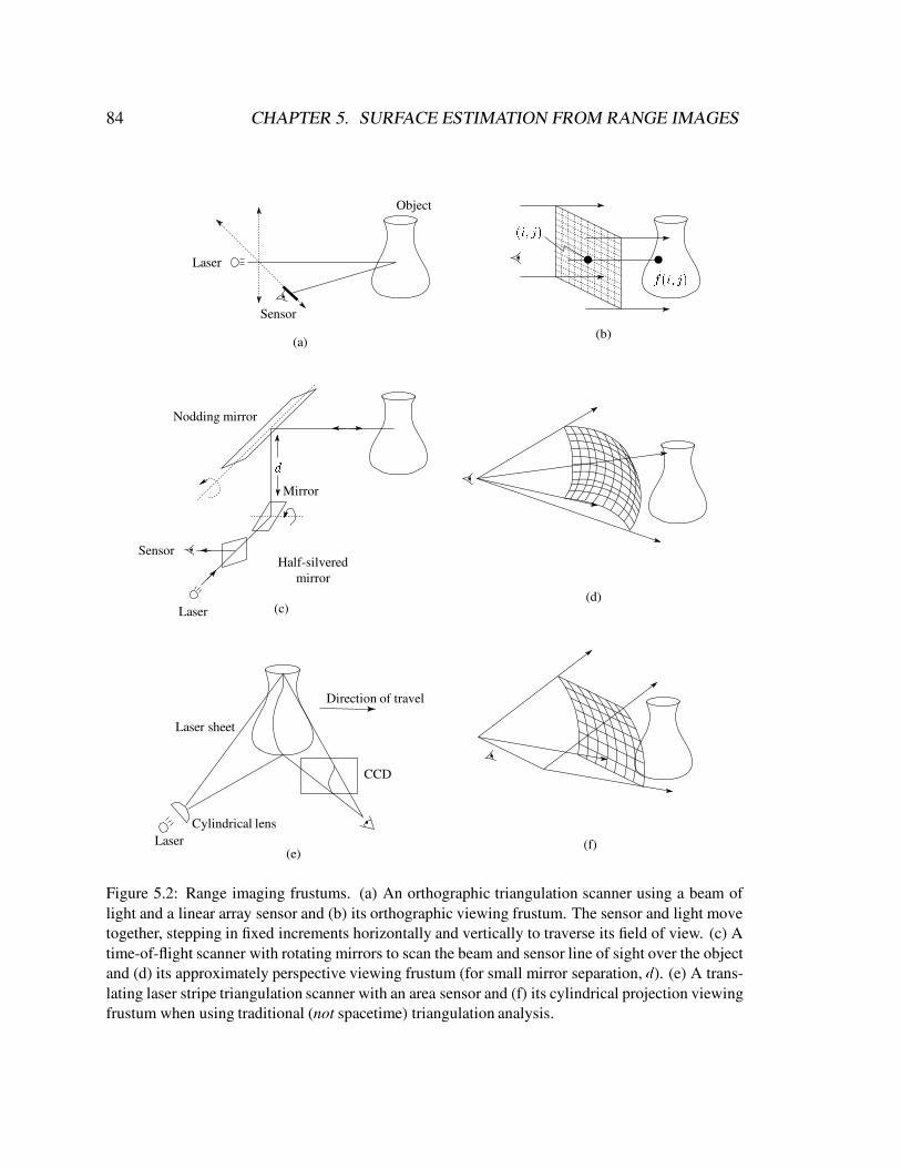
84 CHAPTER 5. SURFACE ESTIMATION FROM RANGE IMAGES
(a)(b)
(c)(d)
(e)(f)
Direction of travel
Object
CCD
LaserCylindrical lens
Laser sheet
Laser
Laser
Sensor
Sensor
Nodding mirror
Mirror
Half-silveredmirror
(i; j)
f(i; j)
d
Figure 5.2: Range imaging frustums. (a) An orthographic triangulation scanner using a beam oflight and a linear array sensor and (b) its orthographic viewing frustum. The sensor and light movetogether, stepping in fixed increments horizontally and vertically to traverse its field of view. (c) Atime-of-flight scanner with rotating mirrors to scan the beam and sensor line of sight over the objectand (d) its approximately perspective viewing frustum (for small mirror separation, d). (e) A trans-lating laser stripe triangulation scanner with an area sensor and (f) its cylindrical projection viewingfrustum when using traditional (not spacetime) triangulation analysis.

5.3. A PROBABILISTIC MODEL 85
Laser
CCD
CylindricalLens
Lasersheet
�r
�ci
Figure 5.3: Range errors for traditional triangulation with two-dimensional imaging. A typical op-tical triangulation system uses a laser beam spread into a diverging sheet of light with a cylindricallens and a CCD that images reflections from within this sheet. Range is usually determined by com-puting the centers of the imaged laser reflections on each scanline. Thus, the errors in determiningthe centers correspond to errors in range that vary along the projections of the scanlines onto thelaser sheet. Notice that the divergence of the laser sheet need not coincide with the divergence of theprojected scanlines.
5.3 A probabilistic model
Before applying a statistical method to estimate the best manifold corresponding to a set of
range images, we first need to define a probabilistic model that describes the likelihood of
any possible manifold. To this end, we seek the probability distribution function (pdf):
pdf(f j f1; � � � ; fp)
where f is a possible manifold approximating the range images ffig. In order to make the
analysis feasible, we make some assumptions about the nature of this pdf . At the end of
this chapter, we will discuss the validity of these assumptions. First, we assume that the
uncertainties in the range images are independent of one another, giving us:

86 CHAPTER 5. SURFACE ESTIMATION FROM RANGE IMAGES
pdf(f j f1; � � � ; fp) =pY
i=1
pdf(f j fi) (5.1)
Next, we assume that sample errors within a range image are independently distributed:
pdf(f j fi) =mYj=1
mYk=1
pdf(f j fi(j; k))
where the range images are of dimension m � m. This independence assumption also re-
quires that the registration of the range images is very accurate. Further, if we consider the
sampling errors to be distributed along the lines of sight of the sensor, then:
pdf(f j fi) =mYj=1
mYk=1
pdf(fi(j; k) j fi(j; k)) (5.2)
where fi(j; k) is the reparameterization of f over the domain of the i’th range image, re-
sampled along the sensor direction at (j; k). Combining Equations 5.1 and 5.2, we have:
pdf(f j f1; � � � ; fp) =pY
i=1
mYj=1
mYk=1
pdf(fi(j; k) j fi(j; k)) (5.3)
Choosing a single function that “best” approximates the range surfaces takes us from
the realm of probability into the realm of statistics.
5.4 Maximum likelihood estimation
One of the most common statistical methods for estimating parameters is the method of
Maximum Likelihood (ML), which chooses the parameter values that maximize a pdf
[Papoulis 1991]. In our case, we seek the surface function, f , that maximizes the pdf
described in Equation 5.3. Note that maximizing the pdf is equivalent to minimizing
� log(pdf), due to the strictly monotonic nature of the logarithm function. Thus, we can
transform our problem to solving for the f that minimizes:
E(f) = �pX
i=1
mXj=1
mXk=1
loghpdf(fi(j; k) j fi(j; k))
i

5.4. MAXIMUM LIKELIHOOD ESTIMATION 87
z = f(x;y)
d1
d2
w2
w1
f2
f1
(x; y; z)
v2
v1
x
y
z
Figure 5.4: Two range surfaces, f1 and f2, are tessellated range images acquired from directionsv1 and v2. In the case of Gaussian statistics, the possible range surface, z = f(x; y), is evaluatedin terms of the weighted squared distances to points on the range surfaces taken along the lines ofsight to the sensor. A point, (x; y; z), is shown here being evaluated to find its corresponding signeddistances, d1 and d2, and weights, w1 and w2.
A difficulty with this formulation, however, is the fact that the function f need only min-
imize the function E(f) for the points that project onto the surface for each sampled range
image. In between these points, the surface need not even be continuous. In fact, the ML
estimate of f would simply be the original points in the range images. Even if we required
continuity, the function f could simply interpolate the points in the range images and be
almost arbitrarily ill-behaved between points. To remedy this problem, we could impose
some continuity and smoothness constraints on the function f . Alternatively, we can inter-
pret the range images as range surfaces; i.e., by suitable interpolation of the range images,
we can generate projected surface estimates of f . Figure 5.4 illustrates this principle. In
this case, the function to minimize becomes:
E(f) =pX
i=1
Z ZAi
g(fi(u; v); ~fi(u; v))dudv (5.4)
where ~fi is the interpolated range surface corresponding to fi, we have replaced� log[pdf()]
with g(), and we have taken the limit of the summation to be an integral. Further, the (u; v)
notation is a parameterization of the sensor’s sampling rays. This parameterization could

88 CHAPTER 5. SURFACE ESTIMATION FROM RANGE IMAGES
pertain to, for example, an (x; y) parameterization in the orthographic case or a (�; �) pa-
rameterization in the perspective case.
One familiar pdf to choose is the Gaussian (normal) distribution:
pdf(fi(u; v) j ~fi(u; v)) = ci(u; v) exp
24�1
2
~fi(u; v)� fi(u; v)
�i(u; v)
!235
where ci is the normalization factor and �i is the standard deviation. The numerator in the
squared term is simply the distance between reconstructed range surface points and points
on the candidate surface, where the distance is taken along the sensing direction:
di(u; v; fi) = ~fi(u; v)� fi(u; v)
Substituting and evaluating � log(pdf), we obtain:
g(fi(u; v); ~fi(u; v)) =1
2wi(u; v)di(u; v; fi)
2 � log(ci(u; v))
where we have set wi(u; v) = 1=�i(u; v)2. Neglecting the additive term that does not de-
pend on f (and thus has no bearing on the minimization ofE(f) with respect to f ), the error
equation becomes:
E(f) =1
2
pXi=1
Z ZAi
wi(u; v)di(u; v; fi)2dudv
Thus, the assumption of Gaussian statistics leads to a weighted least squares minimiza-
tion, where distances are taken between range surfaces and the minimizing function along
range image viewing directions.
Note that the domain of integration in the previous equations depends on the viewpoint
and ray distribution of the sensor. By choosing a common domain of integration, we can
bring the summation under the integral and attempt to minimize E(f) by applying the cal-
culus of variations.

5.5. UNIFYING THE DOMAIN OF INTEGRATION 89
5.5 Unifying the domain of integration
In order to solve for the optimal surface, we would like to put the total error (Equation 5.4)
in a form that resembles:
E(f) =Z Z
A
pXi=1
ei(x; y; f)dxdy
where we have chosen the domain of integration to be the x�y plane over which our candi-
date surface, f(x; y), is a function. The function ei(x; y; f) is the error associated with the
point, (x; y; f), on the surface as measured with respect to the i’th range image.
To help see the connections we need to make, we can rewrite Equation 5.4 as:
E(f) =pX
i=1
Z ZAi
gi(u; v; fi)dudv
where we define gi to be:
gi(u; v; fi) � g(fi(u; v); ~fi(u; v))
Our goal then is to find a relationship between ei and gi through their respective domains:
ei(x; y; f)dxdy? ! gi(u; v; fi)dudv
In fact, part of the connection is already made, because ei and gi are simply reparam-
eterizations of one another; ei is the error at a point, (x; y; f), on the surface, and gi is the
error at the same point, expressed in the coordinates of the sensor, (u; v; fi).
The differentials dxdy and dudv are generally related to one another through the Ja-
cobian. However, rather than compute the Jacobian directly, we prefer to derive the re-
lationship between the differentials explicitly using geometric arguments. The intuitions
gained help in generalizing from the simplest case, orthographic projection, to more arbi-
trary viewing frustums such as line perspective. Thus, we will first consider the case of an
orthographic sensor.

90 CHAPTER 5. SURFACE ESTIMATION FROM RANGE IMAGES
x
y
xj
yj xi
yi
z
zizj
dAj
dAi
dA
z = f(x; y)bx
by
dAf
n
vjvi
Figure 5.5: Differential area relations for reparameterization. Orthographic range images are ac-quired from different viewpoints, yielding surface parameterizations over domains such as (xi; yi)and (xj ; yj). Instead, we want to estimate a surface over a canonical domain (x; y). When inte-grating over this canonical domain, we must relate differential areas in this domain to areas in thedomains of the original range images.
For an orthographic sensor, we must project the area dA = dxdy onto the function
f(x; y), and then re-project it onto the i’th range image’s viewing plane, as indicated in Fig-
ure 5.5. We use Cartesian (xi; yi; zi) coordinates to represent (u; v; fi). First, we note that
moving a unit distance in the x-direction in the (x; y) domain corresponds to moving along
the vector bx on the surface f , where:
bx =
1; 0;
@z
@x
!
Similarly, moving in the y-direction corresponds to moving along by on the surface:
by =
0; 1;
@z
@y
!
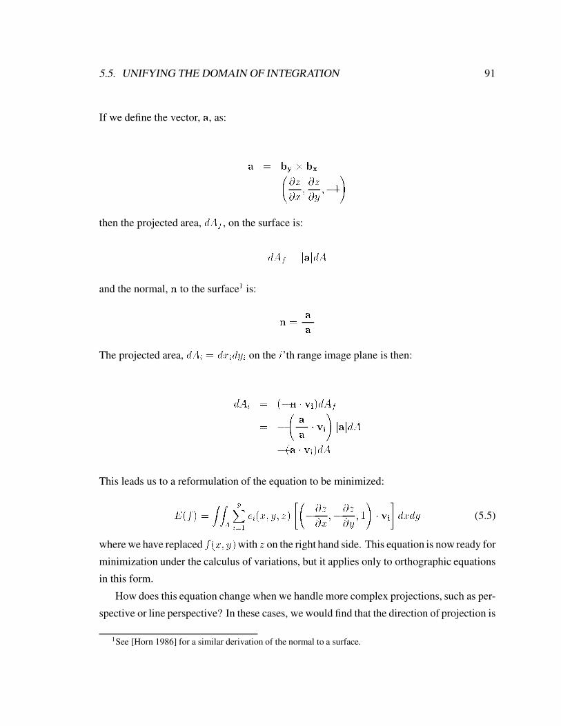
5.5. UNIFYING THE DOMAIN OF INTEGRATION 91
If we define the vector, a, as:
a = by � bx=
@z
@x;@z
@y;�1
!
then the projected area, dAf , on the surface is:
dAf = jajdA
and the normal, n to the surface1 is:
n =a
jaj
The projected area, dAi = dxidyi on the i’th range image plane is then:
dAi = (�n � vi)dAf
= � a
jaj � vi!jajdA
= �(a � vi)dA
This leads us to a reformulation of the equation to be minimized:
E(f) =Z Z
A
pXi=1
ei(x; y; z)
" �@z@x
;�@z@y
; 1
!� vi
#dxdy (5.5)
where we have replaced f(x; y)with z on the right hand side. This equation is now ready for
minimization under the calculus of variations, but it applies only to orthographic equations
in this form.
How does this equation change when we handle more complex projections, such as per-
spective or line perspective? In these cases, we would find that the direction of projection is
1See [Horn 1986] for a similar derivation of the normal to a surface.

92 CHAPTER 5. SURFACE ESTIMATION FROM RANGE IMAGES
not constant as in the orthographic case, but varies over space. Further, the contribution of
a surface element varies not only with the orientation of the element, but also with distance
from the center of projection. For example, as an element moves away from the center of
projection for the perspective case, its apparent size falls off with 1=r2, where r is the dis-
tance from the center.
One approach to the problem might be to define a suitable projection surface that cap-
tures the variation in orientation of projection rays and onto which we can project a surface
element to compute its contribution to the error integral. For example, we could define a
unit sphere about the center of projection for the perspective case. The directions of projec-
tion would run radially, normal to the surface of the sphere, and we could project a surface
element dAf onto the sphere and use this area as the measure of the contribution of the ele-
ment. This definition leads to the measurement dAf in terms of the solid angle it subtends.
This is exactly what we would expect, and it will yield the desired 1=r2 fall-off. For the
line perspective, the projection surface would be a cylinder of unit radius, yielding projec-
tion rays that emanate radially from the center line, and the contribution of a surface element
would fall off as 1=r, where r is the distance from the center line.
While the use of these projection surfaces will work in a number of cases, it is too re-
strictive a definition and will not work in all cases. Instead, we propose an alternative and
more general way of looking at these projections. Consider the two-dimensional case of a
perspective projection as shown in Figure 5.6. The projection rays radiate from the center
of projection. For every point in space (except the center of projection), a single ray passes
through that point in a particular direction. The directions evaluated throughout space de-
fine a vector field as shown in Figure 5.6b. We could then compute the projected length of
a unit line element by dotting the normal of the element with the projection direction at the
center of the element.
The direction field alone, however, does not tell us the contribution the element would
have to an integral over all directions in the projection. This contribution should be a mea-
sure of how many rays cross the a unit line segment in the direction of projection. In our
example, this “ray density” should fall of with the inverse distance from the center of pro-
jection. By weighting our direction field by the “ray density” measure, we arrive at a new

5.5. UNIFYING THE DOMAIN OF INTEGRATION 93
(a)
(c)
(b)
L1
L2
L3
v(x; y)
n
L
Figure 5.6: Ray density and vector fields in 2D. (a) For a perspective projection in 2D, the sensor iseffectively a point source casting rays to sample space. (b) We can view this set of rays as defining avector field, where each point in space has an associated ray direction. The contribution of elementsin the field for the purposes of integration is defined by how many rays pass through the elements;element L1 receives more rays than element L2, because it is closer to the sensor. It also receivesmore rays than L3, because it is more normal to the ray direction. (c) To encode the variations in raydensity, we multiply the direction field in (b) by the ray density. Now the contribution of an elementis jLjn � v(x; y).

94 CHAPTER 5. SURFACE ESTIMATION FROM RANGE IMAGES
vector field, depicted in Figure 5.6c. For a unit line segment, dotting the normal of the seg-
ment with the strength of this vector field will yield the total contribution of the element.
This “ray density” field has a familiar physical interpretation. If we think of the center of
projection as being a point source sending equal amounts of particles in all directions, then
the “ray density” field is the vector flow field describing the direction and rate of particle
flow across unit projected lengths. If we think of these particles as photons, we arrive at a
description of the light field about the point source, and we can measure the contribution of
a surface as the amount of light that flows through the element. We assume the projections
are one-to-one, so the light fields will have a single flow direction at every point.
One of the most important elements of this physical analogy, is the fact that the pro-
jection rays emanate from the sensor, but they flow forever without being extinguished or
created anew in space. In other words, this flow field is conservative at all points outside
of the regions where the rays originate. Further, the projection rays are fixed for each range
scan; i.e., the flow field is static. These conservative and static properties will prove very
useful in the next section.
In general, any range imaging frustum will define a vector field whose directions are
consistent with the projection rays and whose magnitude is equal to the flux of rays crossing
a unit projected area. For the case of an orthographic projection, this vector field is simply
a unit vector in the direction of projection:
v(x; y; z) = v
A perspective projection yields a radial field with 1=r2 fall-off:
v(r; �; �) =r
r2
where r = r=jrj.The line perspective results in a cylindrically radial field with 1=r fall-off:
v(r; �; x) =r
r

5.6. CALCULUS OF VARIATIONS 95
In the latter two cases, we have expressed the vector fields in spherical and cylindrical
coordinates, but they are all equivalently expressible in Cartesian coordinates.
With this new vector flow field analogy, we can now express the relation between dA =
dxdy and the ray differential dAi = duidvi as:
dAi =
�@z@x
;�@z@y
; 1
!� vi(x; y; z)dA
Similarly, the error equation becomes:
E(f) =Z Z
A
pXi=1
ei(x; y; z)
" �@z@x
;�@z@y
; 1
!� vi(x; y; z)
#dxdy (5.6)
This equation is almost identical to Equation 5.5, except that the constant vector vi has been
replaced with a vector field vi(x; y; z). For the special case of Gaussian statistics, this inte-
gral becomes:
E(f) =Z Z
A
pXi=1
wi(x; y; z)di(x; y; z)2
" �@z@x
;�@z@y
; 1
!� vi(x; y; z)
#dxdy (5.7)
Note how the integration over a common domain brings the summation under the in-
tegral. This new formulation allows us to apply the calculus of variations to find the z =
f(x; y) that minimizes the integral.
5.6 Calculus of variations
One of the primary objectives of the calculus of variations is to take an integral of the form:
I =Z Z Z
h
x; y; z;
@z
@x;@z
@y
!dxdydz
and compute the function:
z = f(x; y)
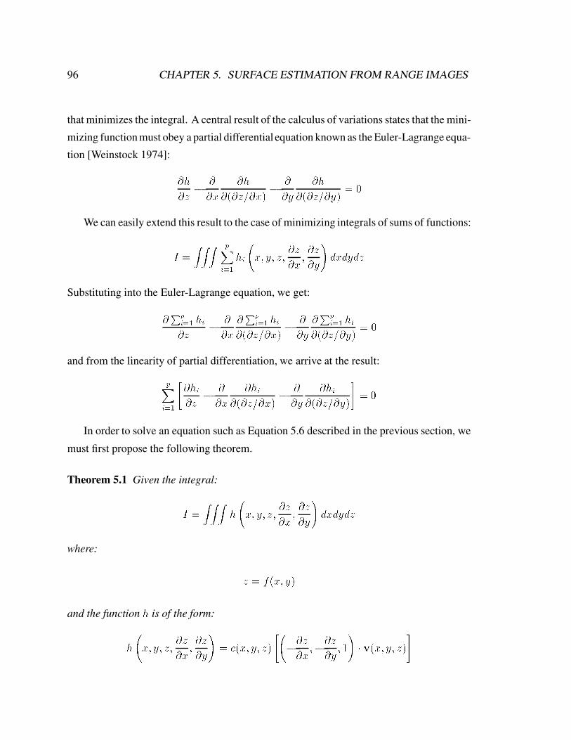
96 CHAPTER 5. SURFACE ESTIMATION FROM RANGE IMAGES
that minimizes the integral. A central result of the calculus of variations states that the mini-
mizing function must obey a partial differential equation known as the Euler-Lagrange equa-
tion [Weinstock 1974]:
@h
@z� @
@x
@h
@(@z=@x)� @
@y
@h
@(@z=@y)= 0
We can easily extend this result to the case of minimizing integrals of sums of functions:
I =Z Z Z pX
i=1
hi
x; y; z;
@z
@x;@z
@y
!dxdydz
Substituting into the Euler-Lagrange equation, we get:
@Pp
i=1 hi@z
� @
@x
@Pp
i=1 hi@(@z=@x)
� @
@y
@Pp
i=1 hi@(@z=@y)
= 0
and from the linearity of partial differentiation, we arrive at the result:
pXi=1
"@hi@z� @
@x
@hi@(@z=@x)
� @
@y
@hi@(@z=@y)
#= 0
In order to solve an equation such as Equation 5.6 described in the previous section, we
must first propose the following theorem.
Theorem 5.1 Given the integral:
I =Z Z Z
h
x; y; z;
@z
@x;@z
@y
!dxdydz
where:
z = f(x; y)
and the function h is of the form:
h
x; y; z;
@z
@x;@z
@y
!= e(x; y; z)
" �@z@x
;�@z@y
; 1
!� v(x; y; z)
#

5.6. CALCULUS OF VARIATIONS 97
the function z that minimizes the integral satisfies the relation:
v � re+ er � v = 0 (5.8)
See Appendix A for the proof. Under the conditions that v(x; y; z) corresponds to a
static, conservative flow field, then the following corollary obtains:
Corollary 5.1 Given the integral:
I =Z Z Z
h
x; y; z;
@z
@x;@z
@y
!dxdydz
where:
z = f(x; y)
and the function h is of the form:
h
x; y; z;
@z
@x;@z
@y
!= e(x; y; z)
" �@z@x
;�@z@y
; 1
!� v(x; y; z)
#
where v(x; y; z) corresponds to a conservative and static vector flow field, then the function
z that minimizes the integral satisfies the relation:
v � re = 0 (5.9)
The proof is straightforward: the divergence of a conservative vector flow field (r � v)
must be exactly zero if the field is not changing with time [Schey 1992]. Thus, the result of
Theorem 5.1 is simplified by removing the divergence term.
Corollary 5.1 has an intuitive interpretation. Consider minimizing the same integral for
a constant vector field (corresponding to an orthographic projection) oriented in the +z di-
rection. The integrand would become h = e(x; y; z) and would not depend on any partials
of z. In this case, the obvious solution would be to minimize with respect to z only; i.e.,
compute:

98 CHAPTER 5. SURFACE ESTIMATION FROM RANGE IMAGES
@e
@z= 0
The only reason h becomes dependent on partials in the theorem, is so that we can solve
the problem over a new domain, rotated with respect to the original domain (for the ortho-
graphic case). The solution in this new domain is actually the same; we take the derivative
along the direction in which the function can vary. We can see this by noting that the dot
product in Equation 5.9 is equivalent to a directional derivative taken along the line of sight
for the original domain.
In order to solve the minimization equation posed in the previous section (Equation 5.6),
we need to extend Theorem 5.1 to minimization over sums of functions. This leads to the
following corollary:
Corollary 5.2 Given the integral:
I =Z Z Z
h
x; y; z;
@z
@x;@z
@y
!dxdydz
where:
z = f(x; y)
and the function h is of the form:
h
x; y; z;
@z
@x;@z
@y
!=
nXi=1
ei(x; y; z)
" �@z@x
;�@z@y
; 1
!� vi(x; y; z)
#
where the vi(x; y; z) correspond to conservative and static vector flow fields, then the func-
tion z that minimizes the integral satisfies the relation:
pXi=1
vi � rei = 0
The proof is a straightforward application of the linearity of the Euler-Lagrange equation
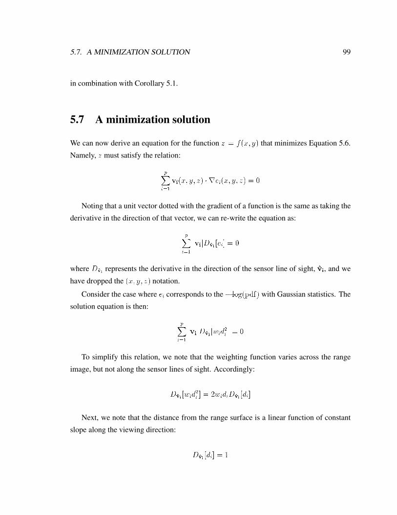
5.7. A MINIMIZATION SOLUTION 99
in combination with Corollary 5.1.
5.7 A minimization solution
We can now derive an equation for the function z = f(x; y) that minimizes Equation 5.6.
Namely, z must satisfy the relation:
pXi=1
vi(x; y; z) � rei(x; y; z) = 0
Noting that a unit vector dotted with the gradient of a function is the same as taking the
derivative in the direction of that vector, we can re-write the equation as:
pXi=1
jvijDvi[ei] = 0
where Dvirepresents the derivative in the direction of the sensor line of sight, vi, and we
have dropped the (x; y; z) notation.
Consider the case where ei corresponds to the� log(pdf) with Gaussian statistics. The
solution equation is then:
pXi=1
jvijDvi[wid
2i ] = 0
To simplify this relation, we note that the weighting function varies across the range
image, but not along the sensor lines of sight. Accordingly:
Dvi[wid
2i ] = 2widiDvi
[di]
Next, we note that the distance from the range surface is a linear function of constant
slope along the viewing direction:
Dvi[di] = 1

100 CHAPTER 5. SURFACE ESTIMATION FROM RANGE IMAGES
Putting these results together, we obtain:
pXi=1
jvijwidi = 0 (5.10)
Thus, we arrive at a surprisingly simple result: the weighted least squares surface is deter-
mined by the zero-isosurface of the sums of the weighted signed distance functions.
In the orthographic case, the value of jvij is unity, so the minimization equation reduces
to:
pXi=1
widi = 0
while for the perspective case, we arrive at:
pXi=1
widir2i
= 0
where the center of projection of the i’th range image is at (xci ; yci ; z
ci ), and:
ri =q(x� xci)2 + (y � yci )2 + (z � zci )2
Note the distinction here between di and ri: di is the distance from a point in 3-space to the
ith range image along the sensor’s line of sight, while ri is the distance from the same point
to the center of projection of the sensor.
5.8 Discussion
We have shown that, under a set of assumptions, the surface of Maximum Likelihood de-
rived from a set of range images can be found as a zero isosurface of a function over 3-space.
The function defined in this domain is a sum of functions generated by each range image,
and thus may be updated one range image at a time. For the case of a weighted least squares
minimization, the optimal surface is the zero isosurface of the sum of the weighted signed
distances along the lines of sight of the range images. Here we review the assumptions and
evaluate the validity of each.

5.8. DISCUSSION 101
All range image samples are statistically independent. Each range image is likely to
have little dependence on the other range images, since they are taken as separate events.
However, whether or not samples within a range image exhibit independence depends on
the range scanning device. Consider a scanner that projects an illuminant on one part of the
surface, records the range, and moves the illuminant to the next sample position. If the il-
luminant projected onto the surface does not overlap with adjacent samples, then we would
expect there to be no statistical correlation among samples. On the other hand, if the illu-
minant does overlap at different positions, then we might expect some correlations. For a
well designed scanner, the illuminant is usually quite narrow, and/or the sensor lines of sight
have little overlap (held tightly in focus), so that any dependence among samples is highly
local, restricted to nearby samples. In this case, we can regard the assumption of statistical
independence as an approximation to the more exact solution that accounts for local sam-
ple interdependence. Still, scanners are likely to have some element of uncertainty that is
independent among samples. Thermal noise in electronic circuitry, for example, will exist
regardless of the proximity of samples, leading to some independent range errors.
Range uncertainties are purely directional and are aligned along the lines of sight of
the sensor which are known to high accuracy. To some extent, this statement may seem to
be a tautology; we have defined a range imaging sensor as a device that returns depth values
along specified lines of sight. When the sensor errs, it returns an erroneous depth, which
must be along the line of sight of the sensor. In the previous chapters, we discussed the
errors in optical triangulation, and these errors manifested themselves along either the lines
of sight of the illuminant or the imaging device, depending what kind of analysis was used in
determining depth. However, a sensor may also have some uncertainty in its lines of sight.
For example, when performing traditional optical triangulation, if a sweeping illuminant has
some “wobble” in its path, then its lines of sight may not be consistent. This inconsistency
would lead to errors in depth along the line of sight, as well as errors that vary side to side,
perpendicular to the line of sight. The error might then take an elliptical form, rather than a
purely directional form. Nonetheless, the devices that control motion can be very precise,
and sensors such as CCD’s have been shown to exhibit excellent geometric stability. As
a result, range imaging sensors can be designed to have excellent accuracy in the lines of
sight, leaving depth uncertainty as the dominant error in the system.

102 CHAPTER 5. SURFACE ESTIMATION FROM RANGE IMAGES
Errors in alignment are much smaller than errors in range samples. The problem
of aligning range images has received a fair amount of attention, and the results indicate
that a number of algorithms can achieve accurate alignment among pairs of range images
[Gagnon et al. 1994] [Turk & Levoy 1994]. Figure 5.7 shows the results of performing
alignment with one of these pairwise methods. The problem of aligning a set of range im-
ages simultaneously, however, requires new alignment algorithms. Consider a set of range
images taken from 8 points on the compass around an object. By aligning the range im-
ages in a pairwise fashion, we can walk around the object. But by the time we have come
full circle, we find that the alignment errors have accumulated, and the first and last range
images are now significantly misaligned. A better approach is to define an error function
that relates all range images to one another, and then minimize this function all at once.
Only recently are solutions to this total alignment problem emerging [Bergevin et al. 1996]
[Stoddart & Hilton 1996]. Nonetheless, through a combination of good initial alignment
and some heuristics for choosing how to perform the pairwise alignments, researchers have
demonstrated that it is still possible to obtain reasonably accurate results. Our results, which
we discuss in Chapter 8, show that the average distance between range samples and their
projections onto the reconstructed surface are roughly the same as the uncertainty in the in-
dividual samples. This fact indicates that range errors dominate the alignment errors.
The range images yield viable range surfaces. While many range scanners generate
a dense grid of depth samples, the analysis in this chapter requires the use of (piecewise)
continuous surfaces. As described earlier, we can use the depth samples to reconstruct the
desired range surfaces. In the case of the spacetime analysis described in the previous chap-
ters, continuous reconstruction of the spacetime volume can indeed lead directly to range
surfaces2. If the surface being sampled is smooth relative to the sampling rate, then the
resulting range surface will be a reasonable estimate of the object’s shape. However, the
apparent smoothness of a surface, changes with viewing direction. A surface viewed at a
grazing angle will be sampled far less than a surface that is facing the sensor. The grazing
angle surface may even be undersampled, yielding a questionable, possibly aliased recon-
struction. To ameliorate this problem, researchers avoid reconstructing the range surface
2In practice, we perform the reconstruction at a fixed resolution, leading to range images that still must beconverted to range surfaces.

5.8. DISCUSSION 103
(a) (b)
(c)
(d)
Figure 5.7: Aligned range images. Two range images were taken 30 degrees apart with an opticaltriangulation scanner. (a) and (b) show the corresponding range surfaces. (c) shows a rendering ofthe two range surfaces after alignment; the surface from (b) is rendered with a darker (red) color.(d) shows a “blow-up” of the head of the model. Note that the range surfaces are so close as to beinter-penetrating across the surface. The RMS error in distances between nearest points on the twosurfaces is on the order of the error in individual range samples, indicating that the majority of theuncertainty remains in sampling error rather than alignment. Note that in some areas of overlap in(c) and (d), one surface is in front of the other in large regions, suggesting correlated range errors.However, these regions are significantly larger than the neighborhoods spanned by the illuminationof the range scanner, making it unlikely that correlation in range errors is the cause. We suspect thesecoherent overlap areas result from small miscalibrations in the range scanner.

104 CHAPTER 5. SURFACE ESTIMATION FROM RANGE IMAGES
in areas that are known to be at sufficiently grazing angles and downweight contributions
from surfaces that are at moderately grazing angles. For example, when using the Gaussian
model with weighted signed distances, we can lower the weights in accordance with the ori-
entation of the surface with respect to the sensor. While this is not strictly consistent with
the notion of variance in Gaussian statistics, it yields excellent results in practice, as we will
show in the following chapters.
In addition, points on the range surface that do not coincide with range samples will not
appear to be statistically independent, even if the range samples are. Consider a 2D world
where our sensor has acquired two neighboring range samples. We can reconstruct the range
surface by linearly interpolating between the two samples, i.e., by connecting them with a
line segment. We may regard the two samples as statistically independent, but the points
on the line segment adjoining them clearly depends on the original samples. While this is
not consistent with the assumption that points on the range surfaces are statistically inde-
pendent, the results do indicate that regarding them as independent is a reasonable approx-
imation.
The range images are functions over the domain where a surface is sought. When
computing the ML optimal surface, we assume that each range image is sampling the same
surface from different points of view. However, an object is generally not a single-valued
function with respect to any single point of view. If we trace a ray from the sensor and
intersect it with the object, we will see the nearest point on the “front” side of the object,
but if we imagine continuing the ray beyond the first intersection, it will eventually intersect
the “back” side of the object. Two different range images will sample the front and back
sides of the object, and clearly they are not seeing the same points. Care must be taken so
that when determining the optimal surface, we do not presume that these two range images
are measuring the same surface. In the next chapter, we discuss efforts to make sure that
opposing surfaces are not treated as the same surface.
In the case of the least squares formulation, the range uncertainties obey Gaussian
statistics. The development in the previous sections is suited to any statistical model for di-
rectional range uncertainty. Nonetheless, Gaussian statistics are appealing because of their
simplicity; in our case, they lead to signed distance functionals. When might this apply? In
some scanners, individual samples are too noisy, so the sampling is repeated along a single

5.8. DISCUSSION 105
line of sight, and the results are averaged. Almost regardless of the statistics of the errors in
the individual samples, averaging them together tends to make the statistics take on a Gaus-
sian character. Indeed, the central limit theorem tells us that the distribution does indeed
become “more Gaussian” with each additional sample included in the average. In addition,
our studies of errors due to laser speckle in optical triangulation indicate that the error dis-
tributions actually do have a Gaussian appearance, as indicated by Figure 4.13.

Chapter 6
A New Volumetric Approach
The discussion in the previous chapter provides a mathematical framework for merging
range images. In this chapter, we begin with a description of how we can implement this
framework on a volumetric grid (Section 6.1). Then, we extend the framework to represent
knowledge about the emptiness of space around an object (Section 6.2). This additional
knowledge leads to a simple algorithm for filling gaps in the reconstruction where no sur-
faces have been observed. In Section 6.3, we analyze sampling and filtering issues that arise
from working with a sampled representation. Finally, we discuss the limitations of the vol-
umetric method described in this chapter and offer some possible solutions (Section 6.4).
6.1 Merging observed surfaces
Our algorithm employs a continuous implicit function, D(x), represented by samples. The
function we represent is the weighted signed distance of each point x to the nearest range
surface along the line of sight to the sensor. We construct this function by combining signed
distance functions d1(x), d2(x), ... dp(x) and weight functions w1(x), w2(x), ... wp(x) ob-
tained from range images 1 ... n. Our combining rules give us for each voxel a cumulative
signed distance function, D(x), and a cumulative weight W (x). We represent these func-
tions on a discrete voxel grid and extract an isosurface corresponding to D(x) = 0. As
shown in the previous chapter, this isosurface is optimal in the least squares sense.
Figure 6.1 illustrates the principle of combining unweighted signed distances for the
106

6.1. MERGING OBSERVED SURFACES 107
(a)
(b)
Sensor
Near
Far
x
Volume
Range surface
Zero-crossing
(isosurface)
Distancefrom
surface
New zero-crossing
x
Figure 6.1: Unweighted signed distance functions in 3D. (a) A range sensor looking down the x-axis observes a range image, shown here as a reconstructed range surface. Following one line ofsight down the x-axis, we can generate a signed distance function as shown. The zero crossing ofthis function is a point on the range surface. (b) The range sensor repeats the measurement, but noisein the range sensing process results in a slightlydifferent range surface. In general, the second surfacewould interpenetrate the first, but we have shown it as an offset from the first surface for purposes ofillustration. Following the same line of sight as before, we obtain another signed distance function.By summing these functions, we arrive at a cumulative function with a new zero crossing positionedmidway between the original range measurements.
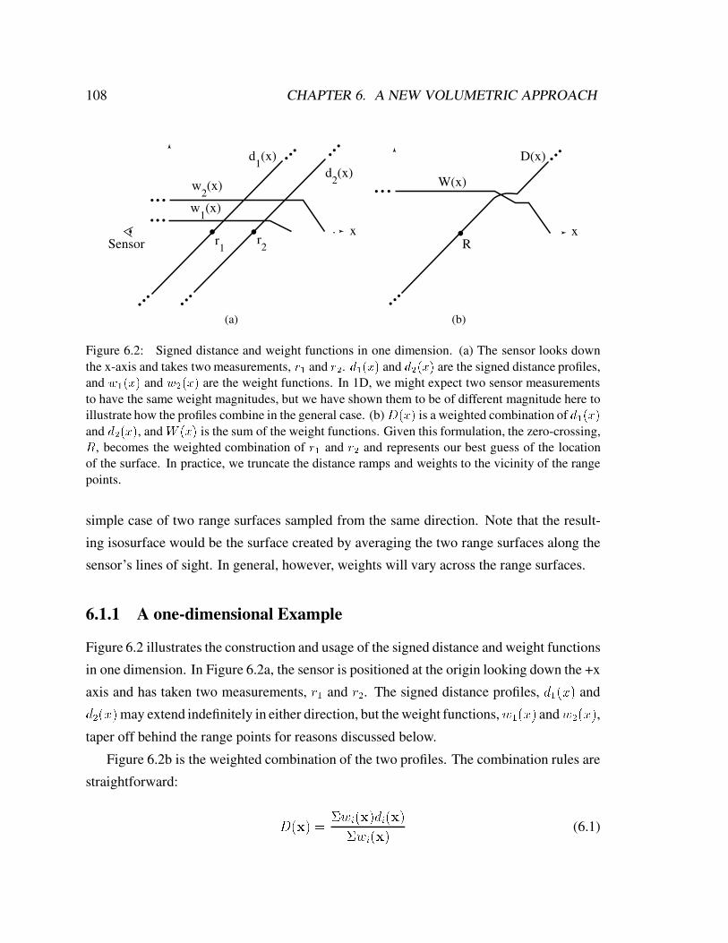
108 CHAPTER 6. A NEW VOLUMETRIC APPROACH
r1
d1(x)
w1(x)
r2
w2(x)
d2(x)
W(x)
D(x)
R
(a) (b)
x xSensor
Figure 6.2: Signed distance and weight functions in one dimension. (a) The sensor looks downthe x-axis and takes two measurements, r1 and r2. d1(x) and d2(x) are the signed distance profiles,and w1(x) and w2(x) are the weight functions. In 1D, we might expect two sensor measurementsto have the same weight magnitudes, but we have shown them to be of different magnitude here toillustrate how the profiles combine in the general case. (b) D(x) is a weighted combination of d1(x)and d2(x), and W (x) is the sum of the weight functions. Given this formulation, the zero-crossing,R, becomes the weighted combination of r1 and r2 and represents our best guess of the locationof the surface. In practice, we truncate the distance ramps and weights to the vicinity of the rangepoints.
simple case of two range surfaces sampled from the same direction. Note that the result-
ing isosurface would be the surface created by averaging the two range surfaces along the
sensor’s lines of sight. In general, however, weights will vary across the range surfaces.
6.1.1 A one-dimensional Example
Figure 6.2 illustrates the construction and usage of the signed distance and weight functions
in one dimension. In Figure 6.2a, the sensor is positioned at the origin looking down the +x
axis and has taken two measurements, r1 and r2. The signed distance profiles, d1(x) and
d2(x)may extend indefinitely in either direction, but the weight functions,w1(x) andw2(x),
taper off behind the range points for reasons discussed below.
Figure 6.2b is the weighted combination of the two profiles. The combination rules are
straightforward:
D(x) =�wi(x)di(x)
�wi(x)(6.1)

6.1. MERGING OBSERVED SURFACES 109
W (x) = �wi(x) (6.2)
where, di(x) and wi(x) are the signed distance and weight functions from the ith range im-
age. Note that settingD(x) = 0 and solving for x is equivalent to the least squares solution
described in the previous chapter. Equation 6.1 differs from Equation 5.10 in that the former
is normalized by the sum of the weights. Since the sum of the weights is always positive, the
equations yield the same isosurface. In practice, we have observed that the normalization
serves to equalize the gradient of the sampled field, D(x), and thereby reduces artifacts in
the isosurface algorithms, which are sensitive to sudden changes in the gradient. We discuss
the benefits of using weighted averages in greater detail in Section 6.3.2.
Expressed as an incremental calculation, the signed distance and weight combination
rules are:
Di+1(x) =Wi(x)Di(x) + wi+1(x)di+1(x)
Wi(x) + wi+1(x)(6.3)
Wi+1(x) = Wi(x) + wi+1(x) (6.4)
where Di(x) and Wi(x) are the cumulative signed distance and weight functions after inte-
grating the ith range image.
In the special case of one dimension, the zero-crossing of the cumulative function is at
a range, R given by:
R =�wiri�wi
(6.5)
i.e., a weighted combination of the acquired range values, which is what one would expect
for a least squares minimization.

110 CHAPTER 6. A NEW VOLUMETRIC APPROACH
6.1.2 Restriction to vicinity of surface
In principle, the distance and weighting functions should extend indefinitely in either di-
rection. However, to prevent surfaces on opposite sides of the object from interfering with
each other, we force the weighting function to taper off behind the surface. There is a trade-
off involved in choosing where the weight function tapers off. It should persist far enough
behind the surface to ensure that all distance ramps will contribute in the vicinity of the fi-
nal zero crossing, but, it should also be as narrow as possible to avoid influencing surfaces
on the other side. To meet these requirements, we force the weights to fall off at a distance
equal to half the maximum uncertainty interval of the range measurements. Similarly, the
signed distance and weight functions need not extend far in front of the surface. Restricting
the functions to the vicinity of the surface also yields a more compact representation and
reduces the computational expense of updating the volume. In Section 6.4.1, we discuss
problems of interfering signed distance ramps in greater detail.

6.1. MERGING OBSERVED SURFACES 111
(b) (c)
(e) (f)
Isosurface
Sensor
n2n1
Dmax
Dmin
(a)
(d)
Sensor
Figure 6.3: Combination of signed distance and weight functions in two dimensions. (a) and (d) arethe signed distance and weight functions, respectively, generated for a range image viewed from thesensor line of sight shown in (d). The signed distance functions are chosen to vary between Dmin
and Dmax , as shown in (a). The weighting falls off with increasing obliquity to the sensor and at theboundaries of the meshes as indicated by the darker regions in (e). The normals, n1 and n2 shownin (e), are oriented at a grazing angle and facing the sensor, respectively. Note how the weighting islower (darker) for the grazing normal. (b) and (e) are the signed distance and weight functions for arange image of the same object taken at a 60 degree rotation. (c) is the signed distance functionD(x)corresponding to the per voxel weighted combination of (a) and (b) constructed using Equations 6.3and 6.4. (f) is the sum of the weights at each voxel, W (x). The dotted green curve in (c) is theisosurface that represents our current estimate of the shape of the object.
6.1.3 Two and three dimensions
In two and three dimensions, the range measurements correspond to curves or surfaces with
weight functions, and the signed distance ramps have directions that are consistent with the
primary directions of sensor uncertainty. Figure 6.3 illustrates the two-dimensional case for
a range curve derived from a single scan containing a row of range samples. In practice, we
use a fixed point representation for the signed distance function, which bounds the values
to lie between Dmin and Dmax as shown in the figure. The values of Dmin and Dmax must
be negative and positive, respectively, as they are on opposite sides of a signed distance
zero-crossing.
For three dimensions, we can summarize the whole algorithm as shown in Figure 6.4.
First, we set all voxel weights to zero, so that new data will overwrite the initial grid values.

112 CHAPTER 6. A NEW VOLUMETRIC APPROACH
/* Initialization */For each voxel {
Set weight = 0}
/* Merging range images */For each range image {
/* Prepare range image */ Tesselate range image Compute vertex weights
/* Update voxels */ For each voxel near the range surface { Find point on range surface Compute signed distance to point Interpolate weight from neighboring vertices Update the voxel’s signed distance and weight }
}
/* Surface extraction */Extract an isosurface at the zero crossing
Figure 6.4: Pseudocode for the method of volumetric integration.
Next, we tessellate each range image by constructing triangles from nearest neighbors on
the sampled lattice. We avoid tessellating over step discontinuities (cliffs in the range map)
by discarding triangles with edge lengths that exceed a threshold. We must also compute a
weight at each vertex as described below.
Once a range image has been converted to a triangle mesh with a weight at each vertex,
we can update the voxel grid. The signed distance contribution is computed by casting a ray
from the sensor through each voxel near the range surface and then intersecting it with the
triangle mesh, as shown in figure 6.5. The weight is computed by linearly interpolating the
weights stored at the intersection triangle’s vertices. Having determined the signed distance
and weight we can apply the update formulae described in Equations 6.3 and 6.4.
At any point during the merging of the range images, we can extract the zero-crossing
isosurface from the volumetric grid. Isosurface extraction algorithms have been well-
explored, and a number of approaches have been demonstrated to produce tessellations
without consistency artifacts [Ning & Bloomenthal 1993]. These algorithms typically de-
compose the volume into cubes or tetrahedra with sample values stored at the vertices, fol-
lowed by interpolation of these samples to estimate locations of zero-crossings, as shown in

6.1. MERGING OBSERVED SURFACES 113
Volume
Sensor
VoxelViewingray
wb
wa
wc
w
Range surface
d
Figure 6.5: Sampling the range surface to update the volume. We compute the weight,w, and signeddistance, d, needed to update the voxel by casting a ray from the sensor, through the voxel onto therange surface. We obtain the weight,w, by linearly interpolating the weights (wa, wb, and wc) storedat neighboring range vertices. Note that for a translating sensor (like our Cyberware scanner), thesensor point is different for each column of range points.
(a)(b)
+
-
+
+ + +
+ +
++
+
- - -
- -
--
-
----
-
-
+
+ +
+ +
+
+ +
- -
-
-
Figure 6.6: Discrete isosurface extraction. (a) In two dimensions, a typical isocontour extractionalgorithm interpolates grid values to estimate isovalue crossings along lattice lines. By connectingthe crossings with line segments, an isocontour is obtained. (b) In three dimensions, the crossingsare connected with triangles. This method corresponds to the marching cubes algorithm describedin [Lorensen & Cline 1987] with corrections in [Montani et al. 1994].

114 CHAPTER 6. A NEW VOLUMETRIC APPROACH
Figure 6.6. The gradients at the extracted zero-crossings provide an estimate of the surface
normals1. We restrict the extraction procedure to skip samples with zero weight, generat-
ing triangles only in the regions of observed data. We will relax this restriction in the next
section.
6.1.4 Choosing surface weights
The choice of weights is theoretically a function of the uncertainties in the range data, but
they can also serve the purpose of manipulating the way range surfaces are merged. As
described in the previous chapter, the use of weighted signed distances corresponds to the
assumption of independent Gaussian statistics along the sensor’s lines of sight. The weight
then is the inverse of the squared variance of the pdf at each point on the surface. In this
sense, the weight represents the degree of confidence in the data; a larger weight means that
the data is more likely to be accurate.
The manner in which weights vary over a surface depend on the scanning technology.
For example, in an optical triangulation system, low intensity images of the laser reflection
imply a lower signal to noise ratio at the sensor, and thus lower confidence in shape esti-
mates. [Soucy & Laurendeau 1995] and [Turk & Levoy 1994] have used this argument to
justify forcing weights to depend on the dot product between the range surface normal and
the laser direction, because the reflected radiance from a diffuse Lambertian surface varies
with this dot product. When applying the spacetime analysis, the “goodness of fit” to the
ideal spacetime Gaussian is also a confidence indicator. If the width of the Gaussian fit to
the data deviates from the ideal width, then the data is accordingly downweighted, or even
discarded. Additionally, at a step discontinuity, range data may be less reliable. The false
edge extensions associated with traditional triangulation illustrate this point. Even in the
case of spacetime analysis, the quality of edges is suspect due to filtering and resolution
limitations.
1If the points xs comprise the implicit surface defined by F (x) = const , then the gradient of F (x) at thesurface, rF (xs), corresponds exactly to the normals over the surface [Edwards & Penney 1982].

6.1. MERGING OBSERVED SURFACES 115
(a) (b)
(c) (d)
Figure 6.7: Dependence of surface sampling rate on view direction. When a surface is viewed “headon” as in (a), the sampling rate is on average significantly higher than when the surface is viewedfrom a grazing angle, as in (b). Note the greater detail in the estimated range surfaces, (c) versus (d).
The variations in weights can also be chosen for very practical considerations. If a sur-
face is roughly planar with some moderate surface detail, then we would expect that a di-
rect view of this surface in line with the predominant surface normal would give a higher
quality range surface than a grazing angle view of the same surface. Figure 6.7 illustrates
this idea. In general, separation between samples on the surface gives an indication of the
comparative sampling rates among different range images. This sample separation is well
approximated by 1= cos where is the angle between the surface normal and the viewing
direction. Thus, by setting the weights to be proportional to cos or even a higher power
(e.g., cos2 ), the contributions from the range surfaces can be biased in favor of range views
with higher surface sampling rates.
Reducing weights near surface boundaries serves a practical purpose as well: smooth
blending of range surfaces. Consider the example in Figure 6.8. If the vertex weights are
not tapered near the boundary of a range surface, then when it is merged with another range
surface, there will be an abrupt jump from the average of two surfaces to a single surface.
By tapering the vertex weights to zero in the vicinity of the boundary of a range surface, this
surface will blend smoothly with other range surfaces.

116 CHAPTER 6. A NEW VOLUMETRIC APPROACH
(a) (b) (c)
Figure 6.8: Tapering vertex weights for surface blending. (a) Two surfaces overlap, but one surface(shown dotted) has a boundary. (b) If the surface weights are not tapered near the boundary, then anabrupt transition appears when merging the surfaces, as indicated by the merged surface (solid line).(c) By tapering the surface weights near the boundary, the surfaces blend smoothly together.
6.2 Hole filling
The algorithm described in the previous section is designed to reconstruct the observed por-
tions of the surface. Unseen portions of the surface will appear as holes in the reconstruction.
While this result is an accurate representation of the known surface, the holes are esthetically
unsatisfying and can present a stumbling block to follow-on algorithms that expect continu-
ous meshes. In [Krishnamurthy & Levoy 1996], for example, the authors describe a method
for parameterizing patches that entails generating evenly spaced grid lines by walking across
the edges of a mesh. Gaps in the mesh prevent the algorithm from creating a fair parame-
terization. As another example, rapid prototyping technologies such as stereolithography
typically require a “watertight” model in order to construct a solid replica [Dolenc 1993].
One option for filling holes is to operate on the reconstructed mesh. If the regions of
the mesh near each hole are very nearly planar, then this approach works well. However,
holes in the meshes can be (and frequently are) highly non-planar and may even require
connections between unconnected components. Instead, we offer a hole filling approach
that operates on our volume, which contains more information than the reconstructed mesh.
6.2.1 A hole-filling algorithm
The key to our algorithm lies in classifying all points in the volume as being in one of three
states: unseen, empty, or near the surface. Holes in the surface are indicated by frontiers be-
tween unseen regions and empty regions (see Figure 6.9). Surfaces placed at these frontiers
offer a plausible way to plug these holes (dotted in Figure 6.9). Obtaining this classifica-
tion and generating these hole fillers leads to a straightforward extension of the algorithm

6.2. HOLE FILLING 117
Unseen
Empty Near surface
W(x) = 0 W(x) > 0
W(x) = 0
Sensor
Unseen
Empty
Observedisosurface
Hole fillisosurface
Nearsurface
(a) (b)
D(x) = Dmin
D(x) = Dmax
min max D < D(x) < D
Figure 6.9: Volumetric grid with space carving and hole filling. (a) The regions in front of the surfaceare seen as empty, regions in the vicinity of the surface ramp through the zero-crossing, while regionsbehind remain unseen. The green (dashed) segments are the isosurfaces generated near the observedsurface, while the red (dotted) segments are hole fillers, generated by tessellating over the transitionfrom empty to unseen. In (b), we identify the three extremal voxel states with their correspondingfunction values.
described in the previous section:
1. Initialize the voxel space to the “unseen” state.
2. Update the voxels near the surface as described in the previous section. As before,
these voxels take on continuous signed distance and weight values.
3. Follow the lines of sight back from the observed surface and mark the corresponding
voxels as “empty”. We refer to this step as space carving.
4. Perform an isosurface extraction at the zero-crossing of the signed distance function.
Additionally, extract a surface between regions seen to be empty and regions that re-
main unseen.
In practice, we represent the unseen and empty states using the function and weight fields
stored on the voxel lattice. We represent the unseen state with the function values D(x) =
Dmax , W (x) = 0 and the empty state with the function values D(x) = Dmin, W (x) = 0,
as shown in Figure 6.9b. The key advantage of this representation is that we can use the
same isosurface extraction algorithm we used in the previous section this time lifting the
prohibition on interpolating voxels of zero weight. This extraction finds both the signed

118 CHAPTER 6. A NEW VOLUMETRIC APPROACH
distance and hole fill isosurfaces and connects them naturally where they meet, i.e., at the
corners in Figure 6.9a where the dotted red line meets the dashed green line. Note that the
triangles that arise from interpolations across voxels of zero weight are distinct from the
others: they are hole fillers. We take advantage of this distinction when smoothing surfaces
as described below.
Figure 6.9 illustrates the method for a single range image, and provides a diagram for the
three-state classification scheme. Figure 6.10 illustrates how the hole filler surfaces connect
to the observed surfaces. The hole filler isosurfaces are “false” in that they are not repre-
sentative of the observed surface, but they do derive from observed data. In particular, they
correspond to a boundary that confines where the surface could plausibly exist. Thus, the
combination of the observed surfaces and the hole fill surfaces represents the object of maxi-
mum volume which is consistent with all of the observations. In practice, we find that many
of the hole fill surfaces are generated in crevices that are hard for the sensor to reach.
6.2.2 Carving from backdrops
We have just seen how “space carving” is a useful operation: it tells us much about the struc-
ture of free space, allowing us to fill holes in an intelligent way. However, our algorithm
only carves back from observed surfaces. There are numerous situations where more carv-
ing would be useful. For example, the interior walls of a hollow cylinder may elude digiti-
zation, but by seeing through the hollow portion of the cylinder to a surface placed behind
it, we can better approximate its geometry. We can extend the carving paradigm to cover
these situations by placing such a backdrop behind the surfaces being scanned. By placing
the backdrop outside of the voxel grid, we utilize it purely for carving space without intro-
ducing its geometry into the model. Figure 6.11 illustrates the utility of space-carving with
backdrops.

6.2. HOLE FILLING 119
D(x,y)
xy
Zoom
Blue: W(x,y) = 0White: W(x,y) > 0
Observedisosurface
Hole fillisosurface
Figure 6.10: A hole-filling visualization. The images represent a slice through the volumetric griddepicted in Figure 6.9. The height of the ramps correspond to the signed distance field, D(x; y),and the shading corresponds to the weight, W (x; y). The isosurface is extracted at the level shown,where the dotted green lines correspond to observed surfaces and the dashed red lines correspondto hole-fill surfaces. Note how the observed and hole-fill surfaces connect seamlessly, with only achange in weights (going to zero at the hole-fill regions) to indicate the transitions.

120 CHAPTER 6. A NEW VOLUMETRIC APPROACH
Backdrop
(c) (d)
(a) (b)
Sensor
Surfaces
Volumetric sliceScanning scenario
Figure 6.11: Carving from backdrops. (a) An orthographic sensor captures a range image of twocylinders. (b) A slice through the volumetric grid after laying down signed distance ramps near theobserved surface and carving out the empty regions in front of the surfaces. It will be difficult to scanthe portions of the cylinders that are close together. (c) The same scene as in (a) with the additionof a backdrop. (b) The volumetric slice after scanning the cylinders with a backdrop placed behindthem. Much more of the space is carved as empty, and the cylinders are clearly segregated by theempty region between them.

6.3. SAMPLING, CONDITIONING, AND FILTERING 121
6.3 Sampling, conditioning, and filtering
Operating in a sampled domain requires attention to several details. In this section, we be-
gin by developing criteria for choosing the voxel resolution. Next, we show how the gradi-
ent variations can introduce artifacts when extracting an isosurface from a sampled volume,
and we develop the notion of a conditioning function to address the problem. Finally, we
describe methods for coping with the aliasing artifacts that arise when extracting hole fill
surfaces.
6.3.1 Voxel resolution and tessellation criteria
Choosing the appropriate voxel resolution is crucial to avoiding aliasing artifacts in the sur-
face reconstruction. Intuitively, the voxel resolution should be sufficient to sample the dis-
tance ramp and should be chosen to match the level of detail of the range surface.
To derive a criterion for the voxel resolution, we examine the problem from a signal pro-
cessing point of view. Combining multiple range surfaces with weighted averages leads to a
complicated analysis that does not offer many insights. Accordingly, we restrict the analysis
to the case of determining the volumetric sampling rate required to represent a single range
surface as a signed distance function. We will consider the role of weights in the context of
isosurfaces in the next section.
In order to estimate the required voxel resolution, we must determine the bandwidth of
the signed distance representation for a range surface. We define the symbols sx, sy , and sz
to correspond to the spatial frequencies in x, y, and z. The radial spatial frequency is then:
�sxsysz =qs2x + s2y + s2z
and we hope to derive an expression for:
�maxsxsysz
�q(smax
x )2 + (smaxy )2 + (smax
z )2
where �maxsxsysz
is the radial bandlimit.
Consider the case of an orthographic sensor looking down the z-axis having acquired a

122 CHAPTER 6. A NEW VOLUMETRIC APPROACH
range surface, f(x; y). For this single scan, the volume will store:
D(x; y; z) = d(z � f(x; y))
where d(z) is the signed distance function centered at z = 0. Taking the Fourier transform:
FfDg =Z Z Z
d(z � f(x; y)) exp[�i2�(sxx+ syy + szz)]dxdxdz
Regrouping the terms, we obtain:
FfDg =Z Z
exp[�i2�(sxx+ syy)]�Z
d(z � f(x; y)) exp[�i2�szz]dz�dxdy
=Z Z
exp[�i2�(sxx+ syy)]Fzfd(z)g exp[�i2�szf(x; y)]dxdy= Fzfd(z)gFxyfexp[�i2�szf(x; y)]g
This equation reveals that the Fourier transform of the signed distance is partially sepa-
rable; i.e., a product of the Fourier transform in z and the transform in xy. The z transform
pertains to a known function, the signed distance ramp, and is thus easily computed. The
xy transform has a significantly more complicated argument that includes the z component
of frequency, sz . Ultimately, we would like to derive the bandwidth of FfDg to help de-
cide the necessary sampling rate for accurate shape capture without aliasing. To do so, we
need to relate some property of the function f(x; y) to the frequency content of the the xy
transform.
One revealing measure that corresponds to bandwidth is the 2D variance of the squared
magnitude of the sxsy spectrum of a function p(x; y) [Bracewell 1986],
(��sxsy )2 �
Z Z(s2x + s2y)jP (sx; sy)j2dsxdsyZ ZjP (sx; sy)j2dsxdsy
(6.6)
where P (sx; sy) is the Fourier transform of p(x; y), and we have assumed the first central

6.3. SAMPLING, CONDITIONING, AND FILTERING 123
moment to be zero. A more convenient definition of this variance arises after the application
of several relations. The first is Rayleigh’s theorem:
Z ZjG(sx; sy)j2dsxdsy =
Z Zjg(x; y)j2dxdy (6.7)
whereG(sx; sy) is the Fourier transform of a function g(x; y). The second two relations are
the rules of Fourier transforms and partial differentiation:
sxG(sx; sy) =�i2�
@
@xg(x; y) (6.8)
syG(sx; sy) =�i2�
@
@yg(x; y) (6.9)
(6.10)
After re-writing Equation 6.6 as
(��sxsy )2 =
Z ZjsxP (sx; sy)j2dsxdsy +
Z ZjsyP (sx; sy)j2dsxdsyZ Z
jP (sx; sy)j2dsxdsy(6.11)
then we can combine Equations 6.7-6.11 to obtain the following relation:
(��sxsy )2 =
1
4�2
Z Z ����� @@xp(x; y)�����2
+
����� @@yp(x; y)�����2
dxdyZ Zjp(x; y)j2dxdy
Now we can make the substitution:
p(x; y) = exp[�i2�szf(x; y)]
which leads to the following expression:
124 CHAPTER 6. A NEW VOLUMETRIC APPROACH
(��sxsy )2 =
s2z
Z ZA
8<:����� @@xf(x; y)
�����2
+
����� @@yf(x; y)�����29=; dxdy
Z ZAdxdy
(6.12)
where A is the area over which the range surface is defined. At the bandlimit, sz obtains its
maximum value smaxz as set by the signed distance function. We can approximate the square
of the overall bandwidth to be:
(�maxsxsysz
)2 � (smaxz )2 + (��sxsy )
2 (6.13)
After noting thatRR
A dxdy = A, we substitute Equation 6.12 into Equation 6.13 to obtain:
(�maxsxsysz
)2 � (smaxz )2
A
Z ZA
8<:1 +
����� @@xf(x; y)�����2
+
����� @@yf(x; y)�����29=; dxdy (6.14)
We can make this relation easier to understand if we define:
hg(x; y)i � 1
A
Z ZAg(x; y)dxdy (6.15)
to be the area average of g(x; y), and we observe that the normal to the surface in the z
direction is (see Section 5.5):
nz(x; y) =�1vuut1 +
����� @@xf(x; y)�����2
+
����� @@yf(x; y)�����2
(6.16)
Combining Equations 6.14-6.16, we arrive at the following relation for the bandwidth of the
surface convolved with the signed distance function:
�maxsxsysz
= smaxz
vuut* 1
jnz(x; y)j2+
In other words, the bandwidth is set by the average square value of the reciprocal of the
component of the surface normal along the viewing direction. It is therefore very sensitive to

6.3. SAMPLING, CONDITIONING, AND FILTERING 125
surfaces at grazing angles to the sensor; i.e., as nz approaches zero, the bandwidth becomes
very large, requiring high sampling rates.
We can derive a simple rule of thumb for the sampling rate if we consider a single planar
surface. In this case, the bandwidth expression simplifies to:
�maxsxsysz
� smaxz
nz
To make this relation useful, we need to know the value of smaxz . We can model the signed
distance function, clipped to have a width of twice the maximum uncertainty interval with
the function:
d(z) = z � rect�z
b
�
where b is width of the distance ramp. The Fourier transform of this function is:
Ffdg = ib
2�
d(sinc(bsz))
dsz
where sinc(x) = sin(�x)=�x. We can define the first zero crossing of this function to be
the bandwidth of the signed distance function. This zero crossing occurs at smaxz = 1=b,
leading to the relation:
�maxsxsysz
� 1
bnz
Thus, the spacing between voxels (�) should be small enough that the sampling fre-
quency (1=�) exceeds the Nyquist sampling rate:
� � bnz2
(6.17)
This relationship provides several insights. First, the voxel spacing must be small enough to
sample the distance ramp adequately, as indicated by the proportionality to the ramp width
b. Less noisy range data requires a narrower distance ramp and a smaller voxel spacing. In
addition, the dependence on nz is closely related to range image tessellation. When a range

126 CHAPTER 6. A NEW VOLUMETRIC APPROACH
image is converted to a range surface, a tessellation criterion determines whether neighbor-
ing range samples should be connected. This criterion typically takes the form of a mini-
mum threshold normal component in the direction of the sensor or a maximum permissible
edge length. The edge length criterion is very similar to the normal component criterion.
Thus, the range surface tessellation criterion enforces a bound on the maximum voxel spac-
ing.
Equation 6.17 can also be seen as a guideline for modifying the distance ramps and tes-
sellation criteria to satisfy a desired sampling rate. In other words, the distance ramp can
be seen as a bandlimiting filter; widening the ramp decreases the required sampling rate.
Applying a more restrictive tessellation criterion has a similar effect.
While Equation 6.17 is based on the unweighted signed distance for a single range im-
age, our experience has shown that it serves as an excellent guide for avoiding aliasing ar-
tifacts even when using weighted averages of signed distances for multiple range images.
6.3.2 Conditioning the implicit function
The algorithm described in this chapter uses a weighted average of the signed distances,
yet in the previous chapter we showed that a simple weighted sum would suffice. In this
section, we show why dividing by the sum of the weights is advantageous.
As shown in the previous chapter, the governing equation for finding a least squares
solution is:
pXi=1
jvi(x; y; z)jwi(x; y; z)di(x; y; z) = 0
Without altering the position of the least squares isosurface, we can multiply this equation
by a strictly positive conditioning function, �(x; y; z):
�(x; y; z)pX
i=1
jvi(x; y; z)jwi(x; y; z)di(x; y; z) = 0
One such conditioning function is the reciprocal of the sum of the weights:

6.3. SAMPLING, CONDITIONING, AND FILTERING 127
0.5
-0.5
0.38
-0.380.26
-0.26
0.14
0.5
-0.5
-0.14
0.02
0.02
(a) (b)
isosurface
actualsurface
Figure 6.12: Tessellation artifacts near a planar edge. (a) A range sensor scans a planar surface upto an edge. (b) The product of the signed distance and the weights are laid down into the volume.The weights taper near an edge causing the value-weight product to shrink. The square markers arevoxels, the dotted line is the actual surface, and the solid line is the extracted isosurface. Note thetessellation artifacts that result from the variations in weight.
�(x; y; z) =1
�wi(x; y; z)(6.18)
which corresponds to computing a weighted average of the signed distances at each voxel.
But what is the utility of a conditioning function? To answer this question, we consider
the impact of tapering weights near mesh boundaries. Figure 6.12 depicts a planar surface
with a boundary edge after being merged into the volumetric grid. Tapering the weights near
the boundary is intended to make for a smoother blend when merging overlapping surfaces,
but the decreasing weights, when multiplied by the signed distance, alter the gradient of
the implicit function. Isosurface extraction methods such as the Marching Cubes algorithm
are very sensitive to variations in the gradient, and the resulting isosurface has artifacts as
depicted in the figure. On the other hand, after dividing by the sum of the weights (for a
single scan, this amounts to unweighted signed distance), the gradient is constant and no
artifacts appear.
Figure 6.13 shows the effect of using sums of weighted distances versus the use of

128 CHAPTER 6. A NEW VOLUMETRIC APPROACH
weighted averages of signed distances when merging range images. Clearly, the weighted
average conditioning smooths the gradient and avoids artifacts associated with the uncon-
ditioned isosurface.
The examples in Figure 6.13 show how the sum of weights conditioning function (Equa-
tion 6.18) can help reduce variations in the gradient to produce better isosurfaces. To see
how we might design different conditioning functions, we can derive an expression for the
gradient magnitude of the conditioned signed distance function:
jrDj =
�����r"�
pXi=1
jvijwidi
#�����=
�����r�nXi=1
jvijwidi + �rpX
i=1
jvijwidi
�����
Since we are only interested in the gradient in the immediate vicinity of the isosurface, the
first term on the right hand side of the last equation vanishes to give:
jrDjiso
=
������rpX
i=1
jvijwidi
�����= �
�����pX
i=1
r (jvijwidi)
�����
where jrDjiso
is the gradient magnitude at the isosurface. Thus, we can ensure a uniform
gradient magnitude in the vicinity of the isosurface by setting the conditioning function to
be:
� =1�����
pXi=1
r (jvijwidi)
�����This observation leads to a uniform gradient algorithm. At each voxel we would store a
scalar and a vector. The scalar would be the cumulative weighted signed distance, and the

6.3. SAMPLING, CONDITIONING, AND FILTERING 129
(c) (d)
(a) (b)
Figure 6.13: Isosurface artifacts and conditioning functions. Noiseless synthetic range images wereconstructed from a perfect sphere scanned orthographically from two directions spaced 45 degreesapart. The scans were merged using two techniques, one with and one without a conditioning func-tion. (a) and (c) are faceted renderings of the resulting isosurfaces, lit to emphasize artifacts. (b) and(d) are the gradient magnitudes across the isosurface. Red areas have small gradients while whiteareas have large gradients. In (a) and (b), no conditioning function is used, and “ripples” appear inthe rendering (a) due to variations in the gradient evident in (b). In (c) and (d), a weighted averageconditioning function is used, and the result is a smooth surface (c) with little variation in the gra-dient (b). The hole at the tops and the jagged boundaries of the reconstructions are artifacts of themarching cubes algorithm operating on the discrete voxel grid used in this illustration.

130 CHAPTER 6. A NEW VOLUMETRIC APPROACH
vector would be the sum of the gradients computed at each voxel for each scan. After merg-
ing a set of scans, we would divide the scalar by the magnitude of the vector at each voxel to
yield a volume with gradients normalized in the vicinity of the isosurface. While we have
yet to implement such an algorithm, it holds promise for minimizing isosurface artifacts due
to gradient magnitude variations.
6.3.3 Mesh filtering vs. anti-aliasing in hole fill regions
Artifacts in the isosurface also arise when applying the method of hole filling by carving
space. Because the transition between unseen and empty is discontinuous and hole fill tri-
angles are generated as an isosurface between these binary states, with no smooth transition,
we generally observe aliasing artifacts in these areas. These artifacts can be eliminated by
pre-filtering the transition region before sampling on the voxel lattice using straightforward
methods such as analytic filtering or super-sampling and averaging down. In practice, we
have obtained satisfactory results by applying another technique: post-filtering the mesh
after reconstruction using weighted averages of nearest vertex neighbors as described in
[Taubin 1995]. The effect of this filtering step is to fair the hole fill surface. Since we know
which triangles correspond to hole fillers, we need only concentrate the surface filtering on
these portions of the mesh. This localized filtering preserves the detail in the observed sur-
face reconstruction. To achieve a smooth blend between filtered hole fill vertices and the
neighboring “real” surface, we allow the filter weights to extend beyond and taper off into
the vicinity of the hole fill boundaries.
6.4 Limitations of the volumetric method
The volumetric method described in this section has several limitations. The first two con-
cern the ability to determine accurate shape from observed surfaces, while the third is a lim-
itation inherent in the process of space carving.

6.4. LIMITATIONS OF THE VOLUMETRIC METHOD 131
(a) (b) (c)
Figure 6.14: Limitation on thin surfaces. (a) A surface is scanned from two sides. (b) The volu-metric grid shows that the distance ramps overlap as the opposing surfaces come close together. (c)The resulting isosurface shows that the interference of signed distance functions results in a thickersurface.
6.4.1 Thin surfaces
As described earlier in this chapter, the width of each signed distance ramp is made as small
as possible while ensuring overlap with ramps taken from the same side of a surface. How-
ever, when opposing surfaces come within a ramp width of each other, then the signed dis-
tances taken from opposite sides of the surface begin to interfere. Figure 6.14 illustrates this
point. In effect, this limitation imposes a minimum thickness of a feature that can be seen
from two sides. This is also problematic for sharp corners. At the tip of a corner, the ad-
joining faces come arbitrarily close together, and opposing scans (i.e., scans that do not see
both sides of the corner) will necessarily interfere with one another in the volume, as show
in Figure 6.16a-c.
The fundamental problem is the inability of the volumetric representation to distinguish
opposing surfaces before combining their distance functions. We may address this prob-
lem in several ways. For instance, we could begin by storing estimated surface normals
for voxels in the neighborhood of the surface. These normals might arise by blending to-
gether estimated normals from individual range scans, though the noisiness of individual
normal estimates will affect results. Alternatively, the normals may be derived from the
initial reconstruction following a recipe such as: (1) reconstruct the surface, (2) reinitial-
ize the volume, (3) deposit the surface normal of the nearest point on the surface into each

132 CHAPTER 6. A NEW VOLUMETRIC APPROACH
D1(x)D2(x)
MIN(D1; D2)x
Figure 6.15: Using the MIN() function to merge opposing distance ramps. Cumulative signed dis-tance functions can be accumulated for differing orientations, as in the case of opposing surfaces.These distance functions are shown here in one dimension. Using theMIN() function to merge thesefunctions before extracting the isosurface will preserve the desired zero crossings.
voxel within the distance ramp of the surface. This second approach assumes that errors as-
sociated with thin surfaces are fairly isotropic; i.e., the erroneous thickening of the surface
is roughly a simple dilation of the surface in the areas affected. Once approximate normals
are established, then we can modify the method for merging range surfaces into the volume.
A simple approach would restrict a range surface to influence only voxels whose normals
are within some threshold of what could possibly be visible to the sensor.
These normal techniques can be extended to store more than one estimated surface nor-
mal and distance function per voxel. For example, if a voxel is between opposing surfaces,
then the algorithm could store the estimated orientations for both of the opposing surfaces
and update separate signed distances for range estimates coming from opposite sides. In
general, storage requirements for this method would vary with the geometry of the object:
in particularly complex regions, storage of multiple estimated normals may be necessary,
whereas smoother regions without opposing surfaces would require only a single normal
and signed distance. To reconstruct the final range surface, it might be possible to follow
the contours of the two signed distances separately, and then merge the resulting geome-
try. Alternatively, these distances could be blended together using a MIN() function before
reconstruction as indicated in Figure 6.15.

6.4. LIMITATIONS OF THE VOLUMETRIC METHOD 133
0.1 -0.7
-0.2
-0.5
0.5
0.3 -0.5
-0.7
-0.2
(a) (b) (c) (d)
Figure 6.16: Limitations due to sharp corners. (a) A corner is scanned from two sides. (b) The vol-umetric grid shows the distance ramps overlapping opposite sides near the apex. (c) The isosurfaceshows a thickening of the corner and a gap at the apex. (d) Samples on the volumetric grid show thateven ideal range data, merged into the volume in a manner avoiding surface thickening will lead toa gap in the reconstruction.
Other potential strategies include modifications to the weight functions. For example, if
the weight functions begin to taper off along the sensor’s line of sight for voxels behind the
range surface, then the interference with the opposing surface will be reduced. However,
when combining surface estimates on the same side of the surface, the tapered weights will
introduce some bias into the reconstruction. Such an approach would affect the accuracy
of the whole reconstruction, but selective application of this strategy might still be of use.
By adjusting the weight profiles for range samples near boundaries, it is possible to reduce
the surface thickening selectively in at least one of the more troublesome areas, i.e., near
corners. Early experiments in this area have yielded promising results.
6.4.2 Bridging sharp corners
Another limitation of the volumetric method is the difficulty in bridging sharp corners, a
problem which persists even if interference of opposing signed distances are eliminated.
Consider the scenario in Figure 6.16. Two scans of a sharp corner acquire accurate descrip-
tions of the corner up to the apex. However, when merging these scans into the volumetric
grid, the restricted marching cubes tessellator cannot “turn the corner” and connect the two
surfaces.
This difficulty is avoidable under two circumstances. If an additional scan observes both
sides of the corner, then the corner is bridged. Alternatively, if the scans of the corner are
observed to be occluding other geometry such as a backdrop, then the space carving step

134 CHAPTER 6. A NEW VOLUMETRIC APPROACH
Figure 6.17: Intersections of viewing shafts for space carving. Three scans are taken from differentpoints of view. The solid green curve is the actual surface. Due to occlusions (not shown), the boundon the object is determined primarily by space carving. Notice that in this two-dimensional example,the resulting boundary is an intersection of empty half-spaces and thus consists of large line segmentswith sizes that do not depend on the voxel resolution.
will declare the region near the apex to be empty. In this case, the hole filling algorithm
will bridge the gap.
In the absence of an additional scan or the use of space carving, however, bridging the
gap is still desirable. The range samples acquired at the apex from two viewpoints may be
arbitrarily close together – even more closely spaced than the samples in individual range
images – so the reconstruction algorithm ought to be able to bridge the gap. One possible
solution would be a modified marching cubes algorithm that assumes regions of the vol-
ume near the surface are empty and performs a local hole-filling only to bridge small gaps.
Alternatively, a different hole-filling algorithm could be applied as a post-process, directly
filling small gaps in the polygonal reconstruction.
6.4.3 Space carving
In many cases, the space carving algorithm described in Section 6.2 can attain a reasonably
tight bound on the object and lead to a plausible hole-free surface. In some cases, however,
the hole-fill regions have undesirable properties. They represent intersections of viewing
“shafts” that may in fact not achieve a tight bound on the surface and may appear as protru-
sions from the object, or, worse, they may change the topological genus of the reconstruction
by introducing “handles”. Figures 6.17, 6.18 and 6.19 illustrate these possibilities.

6.4. LIMITATIONS OF THE VOLUMETRIC METHOD 135
(a)
(b) (c)
Figure 6.18: Protrusion generated during space carving. (a) Four slices through a volumetric gridshow the signed distance ramps due to visible surfaces as well as the resultant space carving. (b) Tak-ing an isosurface that includes hole-filling yields a surface with a protrusion. (c) Red surfaces indi-cate the hole fill regions of the isosurface.
(a)
(b) (c)
Figure 6.19: Errors in topological type due to space carving. (a) Five slices through a volumetricgrid show the signed distance ramps due to visible surfaces as well as the resultant space carving.(b) The resulting isosurface has a “handle”. (c) Red surfaces indicate the hole fill regions of theisosurface.

136 CHAPTER 6. A NEW VOLUMETRIC APPROACH
(a) (b) (c) (d) (e)
?
Figure 6.20: Aggressive strategies for space carving with a range sensor using a single line of sightper pixel. (a) A surface is scanned with a range sensor that has a single line of sight per sample.There is a gap in the recorded range data, which could correspond to the dotted surface. (b) A con-servative strategy would carve space only from the observed surfaces. (c) A very aggressive strategywould incorporate the notion that missing data implies no surface along the sensor’s line of sight. Inthis case, the carving extends to the limit of the sensor’s field of view. (d) Due to sensitivity limita-tions, surfaces at grazing angles to the sensor may not be detected. This places a limit on how muchspace may be declared empty and still be consistent with a surface that just evades detection due tooblique orientation. (e) A still less aggressive strategy would simply fill the gap by bounding theemptiness at the line segment connecting the edges of the missing data. Such a strategy might leadto less objectionable hole fill regions such as would be generated by the indentation shown in (d).
These undesirable hole fillers might be removed at the volumetric level or by operating
on the reconstructed surface. One volumetric approach might be to apply image process-
ing operations such as erosions and dilations to modify the hole fill regions and possibly
collapse thin unknown regions that lead to “handles” such as the one shown in Figure 6.19
[Jain 1989]. In addition, more aggressive space carving strategies could be employed to
empty out more of space as illustrated in Figure 6.20. Consider a very simple range sen-
sor with a single line of sight. If such a sensor were to return no measurement, we would
normally draw no conclusions. In fact, barring a surface that is “invisible” to the sensor,
one can argue that there is no surface along the sensor’s line of sight, or else it would have
been detected. The space must therefore be empty in this direction. For a full range imaging
sensor, we could follow all lines of sight that returned no range data and declare all these
regions of the volume to be empty. In practice, this approach could not be applied indis-
criminately. For instance, no data is returned from very dark regions of a surface or shiny
portions that deflect the line of sight. Even if the surface were known to have a uniform
diffuse reflectance, regions that are oblique to the sensor may not return enough light to be
detected. In this case, there would be a limit to how far the space carving would proceed

6.4. LIMITATIONS OF THE VOLUMETRIC METHOD 137
while being consistent with the possibility that the surface is receding with steep slope. Fig-
ure 6.20 shows how this more aggressive space carving might proceed.
In the case of a triangulation scanner, space carving is complicated by the requirement
that each point must have a clear line of sight to both the laser and the camera. The con-
servative approach consists of following the lines of sight from the surface to both the laser
and the camera and declaring the voxels to be empty as shown in Figure 6.21. For the case
of aggressive space carving, we refer to Figure 6.22. If we hypothesize that point A in Fig-
ure 6.22a is not empty, then there must be a surface that occludes the line of sight of the laser
or the sensor, e.g., point B. But in order for point B to be an occluder, then there must be yet
another surface that blocks its visibility. Following this line of reasoning, we eventually de-
termine that a surface must exist in the region of space already conservatively declared to be
empty in order to prevent the detection of point A. This contradiction leads to the conclusion
that point A must be empty. By induction, we can then argue that all points that are acces-
sible to both the laser and the sensor must be empty [Freyburger 1994]. As with the single
line of sight rangefinder, less aggressive strategies are also possible (Figure 6.22e and f).
Another approach to improving the hole fill regions would be to operate directly on the
polygonal reconstruction. For example, the tangent planes to the surface at the boundary
between the hole fill and the observed surface could be used to coerce the hole fill to relax
into a less protruding configuration. Ideally, such a relaxation procedure could be extended
to modify the topology and collapse undesirable handles in the hole fill regions.

138 CHAPTER 6. A NEW VOLUMETRIC APPROACH
?
(a) (b) (c) (d)
Figure 6.21: Conservative strategy for space carving with a triangulation range sensor. (a) A surfaceis scanned with a triangulation range sensor that has two lines of sight per sample. For the purpose ofillustration, the camera is assumed orthographic and the scanning sweep to be linear. (b) The regionof space that must be empty from the point of view of the laser. (c) The region of space that must beempty from the point of view of the camera. (d) The union of the empty spaces yields a conservativeestimate of the emptiness of space around the observed surfaces.
(a) (b) (c) (d)
(e) (f)
AB
Figure 6.22: Aggressive strategies for space carving with a triangulation range sensor. The sensorgeometry is assumed the same as in Figure 6.21a. (a) Magnified view of the hole fill region estab-lished by conservative space carving in Figure 6.21d. Following the arguments in the text, all pointsthat could be visible to both the laser and the sensor must be empty. (b) The region of space thatcould be empty from the point of view of the laser. (c) The region of space that could be empty fromthe point of view of the camera. (d) The intersection of the empty regions in (b) and (c) yields anaggressive estimate about the emptiness of space around the observed surface. (e) Surfaces at graz-ing angle to the laser or camera might not be detected, so a less aggressive strategy would taper theboundaries of the space carving region. (f) As in Figure 6.20, a less aggressive strategy would sim-ply fill the gap by bounding the emptiness at the line segment connecting the edges of the missingdata.

Chapter 7
Fast algorithms for the volumetric
method
The creation of detailed, complex models requires a large amount of input data to be merged
into high resolution voxel grids. The examples in the next chapter include models generated
from as many as 70 scans containing up to 12 million input vertices with volumetric grids
ranging in size up to 160 million voxels. Clearly, time and space optimizations are critical
for merging this data and managing these grids. In this chapter, we begin by describing a
run-length encoding scheme for efficient storage of the volumetric data (Section 7.1). Next,
we develop a number of optimizations designed to improve execution time when merging
range data into the volume (Section 7.2). In Section 7.3, we summarize an efficient isosur-
face extraction method. Finally, we show that the storage and execution optimizations lead
to significant improvements in asymptotic complexity (Section 7.4).
7.1 Run-length encoding
The core data structure is a run-length encoded (RLE) volume with three run types: empty,
unseen, and varying. The varying fields are stored as an explicit stream data, rather than
runs of constant value. Typical memory savings vary from 10:1 to 20:1. In fact, the space
required to represent one of these voxel grids is usually less than the memory required to
represent the final mesh as a list of vertices and triangle indices.
139

140 CHAPTER 7. FAST ALGORITHMS FOR THE VOLUMETRIC METHOD
(a) (b) (c) (d)
Voxelslices
Volume
Sensor
Resampledrangeimage
Rangeimage
Rangeimage
Figure 7.1: Overview of range image resampling and scanline order voxel updates. (a) Casting raysfrom the pixels on the range image means cutting across scanlines of the voxel grid, resulting in poormemory performance. (b) Instead, we run along scanlines of voxels, mapping them to the correct po-sitions on the resampled range image. (c) Range image scanlines are not in general oriented to allowfor coherently streaming through voxel and range scanlines. (d) By resampling the range image, wecan obtain the desired range scanline orientation.
7.2 Fast volume updating
Updating the volume from a range image may be likened to inverse volume rendering: in-
stead of reading from a volume and writing to an image, we read from a range image and
write to a volume. Research in volume rendering has shown that the manner of traversing
the volume and image is critical to the efficiency of the algorithm [Lacroute & Levoy 1994].
In particular, streaming through the image and following each line of sight through the vol-
ume leads to poor performance, because it requires random access to voxels that are not
adjacent in memory, as shown in Figure 7.1a. We can instead step through the volume in
scanline order, but this requires random access of the image pixels, leading to a similar mem-
ory access inefficiency, as shown in Figure 7.1c. The solution is to pre-warp the image in a
manner that forces voxel and image scanlines to map onto each other.
In this section, we develop the geometric intuition for how the range image plane must
be oriented to ensure ideal scanline alignment for both the orthographic and the perspec-
tive case. Next we describe methods of performing the resampling and subsequent updating
of the volume. Obeying the more restrictive image plane requirement imposed by the per-
spective case, we show how we can develop a shear-warp method for resampling the range
image and updating the volume. This shear-warp method leads to a fast algorithm using bi-
nary depth trees to update only relevant portions of the volume. Finally, we describe a fast

7.2. FAST VOLUME UPDATING 141
(a) (b)
Voxel grid
Range image plane Sensor
vvox
vimvproj
Figure 7.2: Orthographic range image resampling. As shown in (a), the voxel scanlines run in thedirectionvvox. The projections of these scanlines onto the range image plane run along the directionvproj, while the range image scanlines run in the direction vim. By rotating the range image planeas shown in (b), we can align the directions of the projected voxel scanlines and the image scanlines.This affords coherent memory access when streaming through the voxel grid and the range image.
transpose method for ensuring that voxel scanlines run parallel to image scanlines.
7.2.1 Scanline alignment
The type of viewing frustum for a rangefinder imposes constraints on how to choose the
range image resampling that guarantees volume and image scanline alignment. For an or-
thographic frustum, the desired alignment can be attained by simply rotating the image plane
about the axis defined by the viewing direction. The amount of rotation can be determined
by projecting the direction of the voxel scanlines onto the image plane, followed by rotat-
ing the image plane until the image scanlines align with the projected viewing directions
(see Figure 7.2). Because the orthographic projection of the voxel scanlines is a set of par-
allel lines, it is always possible to rotate the range image about the view direction to assure
mutual alignment of image and voxel scanlines.
Perspective viewing frustums impose additional constraints. The first requires that the
new image plane be parallel to the voxel scanlines. Figure 7.3 shows how this constraint

142 CHAPTER 7. FAST ALGORITHMS FOR THE VOLUMETRIC METHOD
Voxel grid
Range image plane
Sensor
vvox
vim
vproj
(a) (c)(b)
Figure 7.3: Perspective range image resampling. The notation follows that of Figure 7.2. In (a), therange image plane is at an angle to the front face of the voxel grid. As a result, the projected voxelscanlines are not parallel. By rotating the image plane so that the image plane is parallel to the voxelscanlines (b), we force the projected voxel scanlines to be parallel. As in the orthographic case, wemust additionally rotate the image plane about the viewing axis to complete the mutual alignment.
applies. When coupled with rotating the image about the viewing axis, the resulting im-
age scanlines, viewed as lines segments in three dimensions, now run exactly parallel to
the voxel scanlines. An additional restriction applies to the direction of the voxel scanlines.
Consider the case shown in Figure 7.4. As we follow the voxel scanlines away from the
viewpoint, the projections of these scanlines progress toward the center of the image. Thus,
no rotation of the image plane is suitable to align voxel and image scanlines. On the other
hand, by reorganizing the voxel scanlines so that they run parallel to the image plane (i.e.,
by transposing the data structure), we obtain the desired alignment.
More complex viewing frustums can make it impossible to assure precise alignment of
voxel and image scanlines, as is the case with the line perspective of the Cyberware scanner
for traditional triangulation. In this case, we can choose an image orientation that is aligned
with scanlines for one voxel slice, but the scanlines at different slices will project to curves
that cross image scanlines. Nevertheless, if the projection is nearly orthographic, i.e., the
rays are not severely divergent, then an image orientation can be chosen to minimize the
amount that projected scanlines cross range image scanlines. If rays are highly divergent,
then other methods, such as partitioning the range image resamplings into manageable sec-
tions may be applicable.

7.2. FAST VOLUME UPDATING 143
Voxel grid
Range image plane
Sensor
vvox
vim
(a) (b)
vproj
Figure 7.4: Transposing the volume for scanline alignment. The notation follows that of Figure 7.2.The projected voxel scanlines in (a) converge to the perspective vanishing point on the image plane.In this case, it is not possible to rotate the image plane to align with projected voxel scanlines. Bytransposing the volume (b), we see that the projected scanlines are now parallel.
7.2.2 Resampling the range image
To resample the range image using the newly oriented image plane, we first reconstruct the
range surface. Next, we can cast a set of rays from the sensor through the image pixels and
intersect them with the range surface. The distances along these rays are the range values to
be stored in the new range image. By interpolating the weights at the vertices on the range
surface, we can associate a new weight with each sample.
Alternatively, we can resample the range image using an incremental scan-conversion
algorithm, a method know to be very efficient. In this case, we first transform the vertices
of the range surface using the viewing transformation specific to the lines of sight of the
range sensor and the image plane. The weights are then assigned as vertex “colors” to be
linearly interpolated during the rendering step, an approach equivalent to Gouraud shading
of triangle colors [Foley et al. 1992]. This resampling can be performed with a traditional
z-buffered rendering algorithm, though no depth comparisons are necessary when entering
values into the z-buffer (i.e., there must be exactly one depth per line of sight if the viewing
rays are properly calibrated).

144 CHAPTER 7. FAST ALGORITHMS FOR THE VOLUMETRIC METHOD
7.2.3 Updating the volume
To merge the range data into the voxel grid, we stream through the voxel scanlines in order
while stepping through the corresponding scanlines in the resampled range image. We map
each voxel scanline to the correct portion of the range scanline as depicted in Figure 7.1b,
and we resample the range data to yield a distance from the range surface. Using the combi-
nation rules given by Equations 6.3 and 6.4, we update the run-length encoded structure. To
preserve the linear memory structure of the RLE volume (and thus avoid using linked lists
of runs scattered through the memory space), we read the voxel scanlines from the current
volume and write the updated scanlines to a second RLE volume; i.e., we double-buffer the
voxel grid.
7.2.4 A shear-warp factorization
In Section 7.2.1, we showed that forcing the range image scanlines to run parallel to the
voxel scanlines is necessary for achieving good memory performance for perspective pro-
jections. If we require that this restriction holds in all cases (including orthography), then we
can develop a shear-warp factorization of the viewing transformation, similar to the one de-
scribed for volume rendering in [Lacroute & Levoy 1994]. The resulting algorithm utilizes
a z-buffered scan-conversion algorithm and allows for computation of signed distances by
comparing a scanline’s constant z value against the resampled z values from the range im-
age. This method of establishing signed distance will be exploited for more efficient voxel
traversal using the binary depth trees described in the next section.
Figure 7.5 illustrates the shear warp procedure for an orthographic projection in two di-
mensions. We first transpose the voxel data structure so that the scanlines run as close to
perpendicular to the viewing direction as possible. Then we shear both the range surface and
voxel grid so that the viewing rays run perpendicular to the voxel slices. Note that shearing
the voxel grid simply amounts to changing the origins of the voxel slices; no resampling of
the voxels is ever performed. Next, we resample the range surface with respect to an image
plane parallel to the voxel slices. As before, we stream through voxel scanlines and resam-
ple depths stored in the resampled range image. The difference between the z-depth of each
voxel (constant within a scanline) and the resampled range depth corresponds to the signed
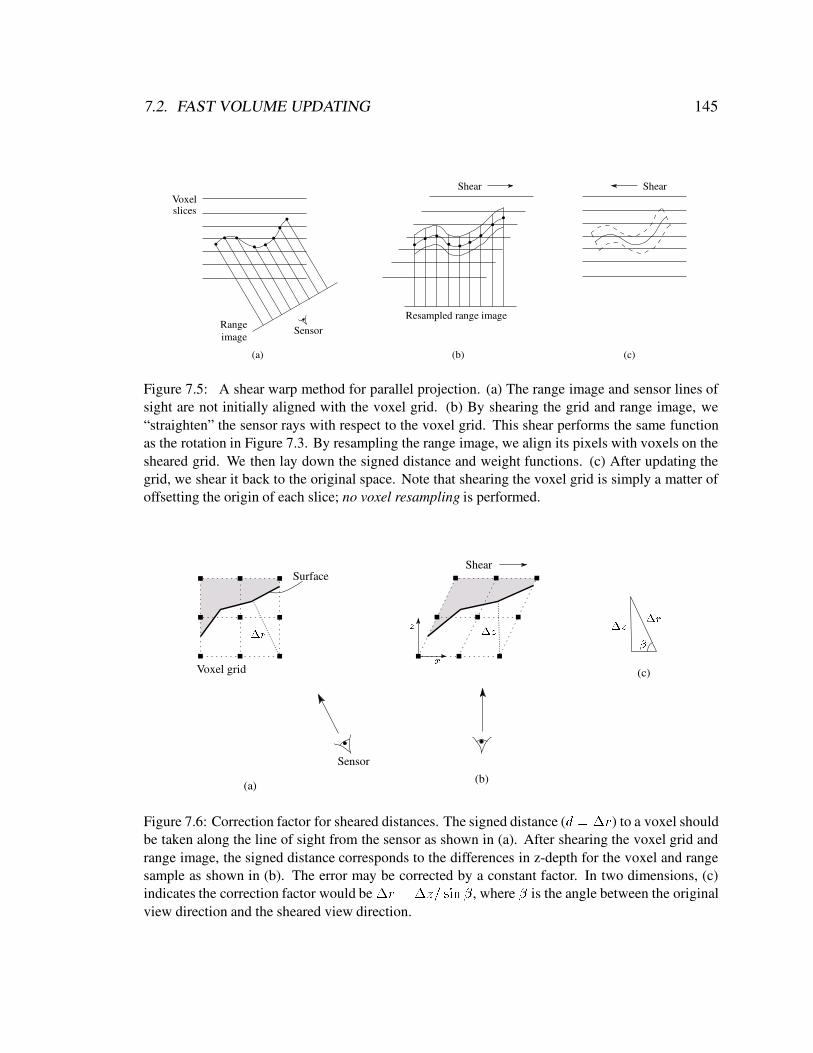
7.2. FAST VOLUME UPDATING 145
(b) (c)
Voxelslices
Resampled range image
Shear Shear
Sensor
(a)
Rangeimage
Figure 7.5: A shear warp method for parallel projection. (a) The range image and sensor lines ofsight are not initially aligned with the voxel grid. (b) By shearing the grid and range image, we“straighten” the sensor rays with respect to the voxel grid. This shear performs the same functionas the rotation in Figure 7.3. By resampling the range image, we align its pixels with voxels on thesheared grid. We then lay down the signed distance and weight functions. (c) After updating thegrid, we shear it back to the original space. Note that shearing the voxel grid is simply a matter ofoffsetting the origin of each slice; no voxel resampling is performed.
Sensor
Voxel grid
Surface
(a)(b)
(c)
Shear
��r �z
�r�z
x
z
Figure 7.6: Correction factor for sheared distances. The signed distance (d = �r) to a voxel shouldbe taken along the line of sight from the sensor as shown in (a). After shearing the voxel grid andrange image, the signed distance corresponds to the differences in z-depth for the voxel and rangesample as shown in (b). The error may be corrected by a constant factor. In two dimensions, (c)indicates the correction factor would be �r = �z= sin �, where � is the angle between the originalview direction and the sheared view direction.

146 CHAPTER 7. FAST ALGORITHMS FOR THE VOLUMETRIC METHOD
(b) (c) (d)(a)
Voxel slices
Rangeimage Sensor
Rangesurface
scale(z)shear
Figure 7.7: Shear-warp for perspective projection. (a) The range surface and sensor lines of sight arenot initially aligned with the voxel grid. By shearing the voxel grid and range surface (b), followedby a depth dependent scale (c), we “straighten” the sensor rays with respect to the voxel grid. (d)After updating the grid, we “unscale” and “unshear” it back to the original space.
distance between the voxel and the range surface. Due to the shear, this distance must be
corrected by a multiplicative factor as depicted in Figure 7.6.
Shear warp factorizations may be adapted to other range imaging frustums as well. Fig-
ure 7.7 shows how a perspective transformation can be decomposed into a shear and a scale.
Again, the voxel lattice is never resampled; the shear and scale only serves to indicate how
voxels map onto the resampled range image plane. The differences between voxel depths
and resampled range depths again correspond to signed distances between the voxel and
the range surface. As with the orthographic case, a correction factor is necessary due to the
differences between the projection direction and viewing rays. This correction factor is not
constant over all viewing rays, but it is constant along each viewing ray. Thus, the correction
factor may be stored at each resampled range image pixel.
More complex imaging frustums such as the line perspective of Figure 5.2f will require
more complex transformations, but the principle of doing modified z comparisons is still
valid and leads to an efficient algorithm with the help of the binary depth tree described in
the next section.

7.2. FAST VOLUME UPDATING 147
Scanline B
Scanline A
Scanline B
Scanline B
(a)
(b)
(c)
Range surface
Range surface
Range surface
Figure 7.8: Binary depth tree. Each pair of resampled range image scanlines is entered into a binarydepth tree. (a) Level 0: a bound is set on the whole range surface. Scanline A is well in front of thebounds and is not processed. Scanline B intersects and forces further traversal of the tree. (b) Level1: the surface is split in two and yields tighter bounds. Still, both sides must be traversed further. (c)Level 2: the surface is quartered and scanline B is found to intersect the first and third quarters.
7.2.5 Binary depth trees
We can take advantage of the fact that z values are constant at each voxel scanline in order
to process the voxels efficiently. In the case of merging range data only in the vicinity of the
surface, we try to avoid processing voxels distant from the surface. To that end, we construct
a binary tree of minimum and maximum depths for every adjacent pair of resampled range
image scanlines. The trees must span pairs of range scanlines, because voxel scanlines may
fall between range scanlines, and linear interpolation requires simultaneously processing
two neighboring scanlines. Figure 7.8 illustrates the binary tree for three levels in two di-
mensions. Before processing each voxel scanline, we query the binary tree to decide which
voxels, if any, are near the range surface. In figure 7.8a, scanline A lies completely outside
of the range tree and thus requires no processing. Scanline B on the other hand does inter-
sect the tree, so we proceed down the levels of the tree until we establish which portions of
the scanline need to be updated. In a similar fashion, the depth tree can be traversed in a

148 CHAPTER 7. FAST ALGORITHMS FOR THE VOLUMETRIC METHOD
manner that rapidly indicates what sections of a scanline are likely to be empty. The result-
ing speed-ups from the binary tree are typically a factor of 15 without carving, and a factor
of 5 with carving.
When using the more complex viewing frustums such as line perspective, the voxel
scanlines may map onto more than two range image scanlines. In this case, the domain of
the binary tree is widened to span as many scanlines as necessary.
7.2.6 Efficient RLE transposes
As described in Figure 7.4, if the scanlines of the volume are badly aligned with the range
image scanlines, it may be necessary to transpose the direction of the scanlines. Without op-
timizations, this transpose would requireO(n3) operations for a volume n voxels on a side.
To avoid this O(n3) cost, the solution is to work primarily on the varying voxels and to cre-
ate the transposed volume directly in RLE form without ever expanding it in an intermediate
step. This objective is very similar to the one for rotation of the RLE spacetime images de-
scribed in Chapter 4. Indeed, the transpose is very much like a rotation by 90 degrees. The
key differences are: (1) no reconstruction and resampling is required, and (2) there are two
values for constant runs (unseen and empty) instead of one (zeroes). The first difference
simplifies the task, while the second complicates it. In the RLE rotation algorithm, when a
run of varying type began where there had been none before on a target scanline, then the
prior run on the target scanline was deduced to be a constant run of zeroes, and could be up-
dated accordingly. As a result, we could stream through only the varying runs in the source
image, and ignore the constant runs. However, when more than one constant run type is
possible, then the constant runs require further attention.
Fortunately, by tracking two source scanlines simultaneously, we can overcome this dif-
ficulty. As before, we construct the target scanlines as we stream through the source scan-
lines. This time, however, each target scanline must keep track of values (empty or unseen)
when building constant runs. As long as the runs in the source scanline are the same as the
current runs in the target scanlines, we would like to skip to the interesting voxels. When
the type of run in the source scanline does differ from the type in the target scanline, then
the target needs to be updated and a new run begun. By simultaneously streaming through

7.3. FAST SURFACE EXTRACTION 149
skip skipcopy
voxels
Empty Unseen
Empty Unseen
Previous
Current
Target scanlinedirection
Source scanline
direction
Empty
skip
Empty
Finish old runStart new runCopy voxel
Figure 7.9: Fast transpose of a multi-valued RLE image. The source scanline direction runs hori-zontally and the target direction runs vertically. We stream through the current and previous sourcescanlines simultaneously. We can skip over intervals where scanlines have constant runs of the samevalue, as indicated with the first “empty” run. When the runs differ, then the target scanline must befinished with its run, so we compute the length of the concluded run, and begin a new one. Whenthe runs are both of varying type, then the varying voxels are simply copied into the target runs.
the current and the previous source scanline, we can deduce when the source is different
from the target, requiring some work to be done. Figure 7.9 illustrates the fast transpose
algorithm.
7.3 Fast surface extraction
To generate our final surfaces, we employ a Marching Cubes algorithm [Lorensen & Cline
1987] with a lookup table that resolves ambiguous cases [Montani et al. 1994]. To reduce
computational costs, we only process voxels that have varying data or are at the boundary
between empty and unseen. A practical consequence of using the hole filling approach is
the generation of spurious components where the lines of sight carved around unknown re-
gions that are not connected to the observed surface. It is a straightforward matter to remove
these components. In practice, we typically work with models that consist of a single, large
connected component. In this case, it suffices to extract the largest connected component.
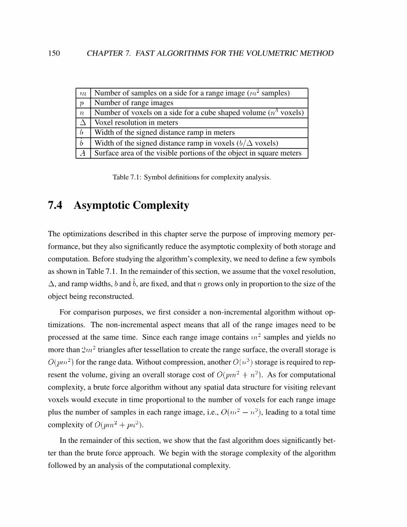
150 CHAPTER 7. FAST ALGORITHMS FOR THE VOLUMETRIC METHOD
m Number of samples on a side for a range image (m2 samples)p Number of range imagesn Number of voxels on a side for a cube shaped volume (n3 voxels)� Voxel resolution in metersb Width of the signed distance ramp in metersb Width of the signed distance ramp in voxels (b=� voxels)A Surface area of the visible portions of the object in square meters
Table 7.1: Symbol definitions for complexity analysis.
7.4 Asymptotic Complexity
The optimizations described in this chapter serve the purpose of improving memory per-
formance, but they also significantly reduce the asymptotic complexity of both storage and
computation. Before studying the algorithm’s complexity, we need to define a few symbols
as shown in Table 7.1. In the remainder of this section, we assume that the voxel resolution,
�, and ramp widths, b and b, are fixed, and that n grows only in proportion to the size of the
object being reconstructed.
For comparison purposes, we first consider a non-incremental algorithm without op-
timizations. The non-incremental aspect means that all of the range images need to be
processed at the same time. Since each range image contains m2 samples and yields no
more than 2m2 triangles after tessellation to create the range surface, the overall storage is
O(pm2) for the range data. Without compression, another O(n3) storage is required to rep-
resent the volume, giving an overall storage cost of O(pm2 + n3). As for computational
complexity, a brute force algorithm without any spatial data structure for visiting relevant
voxels would execute in time proportional to the number of voxels for each range image
plus the number of samples in each range image, i.e., O(m2 + n3), leading to a total time
complexity of O(pm2 + pn3).
In the remainder of this section, we show that the fast algorithm does significantly bet-
ter than the brute force approach. We begin with the storage complexity of the algorithm
followed by an analysis of the computational complexity.

7.4. ASYMPTOTIC COMPLEXITY 151
7.4.1 Storage
To analyze storage complexity, we first consider the costs of storing the original range im-
ages as well the resampled range images and their depth tree data structures. Next we exam-
ine the storage requirements for the RLE volume with and without space carving. Finally,
we compute the storage costs of the reconstructed surface and compare it to the volumetric
storage costs.
As described above, each range image contains m2 samples resulting in no more than
2m2 triangles after tessellation. Because the volumetric algorithm is incremental, we need
not hold all range images in memory at once, so the storage cost for manipulating the range
images isO(m2). Before merging the range surface into the volume, it is resampled at voxel
resolution. This resampled range image requiresO(n2) storage. In addition, a binary tree is
associated with each scanline of the resampled range image. After summing over the nodes
of one tree, we find that it holds no more than 2n nodes, leading to a total of 2n2 nodes over
the whole resampled range image. Thus, the storage cost for the resampled range image and
its binary trees is O(n2).
When reconstructing the observed portions of the surface without space carving, the sur-
face is effectively “blurred” into the volume by the signed distance ramps. This blurred sur-
face occupies a volume of roughly V = bA, which translates to bA=�3 or bA=�2 voxels
that must be stored. The RLE representation requires additional storage for the run lengths.
If the average number of intersections of the surface with each voxel scanline is csurf\ , then
(1 + 2csurf\ )n2 run lengths are necessary. The overall storage cost for the volumetric data
structure is then O(bA=�2 + (1 + 2csurf\ )n2). For objects that do not have an unusually
high surface area to volume ratio (i.e., objects without many folds or spiny projections),
then A=�2 � n2 and the number of voxels required is proportional to bn2. Thus, for non-
pathological surfaces, the storage cost for regions near the observed surface is O(n2).
The addition of space carving to the algorithm has the potential of greatly increased stor-
age costs. When a sequence of voxels are all labeled empty, they are compactly stored as a
single run of empty voxels; however, the examples in Figure 7.10 illustrate some pathologi-
cal cases that defy efficient storage. The objects in this figure have highly complex geometry
(7.10a) or extreme variations in surface reflectance (7.10b) that can lead to the creation of

152 CHAPTER 7. FAST ALGORITHMS FOR THE VOLUMETRIC METHOD
(a) (b)
Figure 7.10: Carving from “difficult” surfaces. (a) The scene contains multiple objects shown ingray. Black regions are seen to be empty. After scanning from two viewpoints, many unseen “is-lands” form. (b) The same as (a), but now there is a single object with regions of negligible re-flectance, shown in dark gray. The sensor cannot digitize these dark portions of the surface, andspace carving from observed surfaces again leads to a fragmented volume.
many thin shafts of emptiness when carving away from the observed surface. The inter-
sections of these shafts can lead to many separate unknown regions. This high degree of
inhomogeneity leads to a worst case storage requirement of O(n3).
Nevertheless, many objects of interest do not exhibit such complexity in geometry or
variations in surface reflectance. More “accessible” objects, i.e., objects having large con-
nected visible portions, lead to a much more efficient representation. In practice, experi-
ments with several objects of moderate complexity show that the storage requirements do
not rise appreciably when including the space carving.
Note that the use of a backdrop can have an appreciable effect on the storage complexity.
Consider the example in Figure 7.11a. Even though the scene being scanned is fairly simple,
the number of unseen “islands” can increase rapidly with the number of scans. However,
by performing only two scans with a backdrop, as shown in Figure 7.11b, these islands do
not appear.
In the last step of the algorithm, we perform an isosurface extraction using an efficient
Marching Cubes algorithm. By processing the run length encoded data structure without
expanding it into the full volume, the cost of storing the volume remains the same as above.
The resulting isosurface will have roughly A=�2 vertices and 2A=�2 faces. In practice,

7.4. ASYMPTOTIC COMPLEXITY 153
(a) (b)
Figure 7.11: Storage complexity with and without backdrops in 2D. Three circles are being scannedindicated as the gray regions. (a) After taking 8 scans without a backdrop, a large number of unseenislands appear. These will result in high storage costs. In fact, more scans can actually increasethe fragmentation. (b) Using a backdrop, only two scans are necessary to declare most of the spacearound the object to be empty.
we have found that the storage required for the RLE volume is comparable to the storage
required for the extracted isosurface.
In summary, for non-pathological cases, the storage requirements for the fast volumetric
algorithm are O(m2 + n2). This complexity is clearly superior to the storage requirement
of O(pm2 + n3) for a non-incremental, uncompressed algorithm.
7.4.2 Computation
The key operations that influence the computational complexity of the volumetric method
are:
� tessellating and resampling the range images
� building the binary depth trees
� performing volume transposes
� finding relevant voxels to update

154 CHAPTER 7. FAST ALGORITHMS FOR THE VOLUMETRIC METHOD
� merging runs of voxels
� extracting the isosurface.
We address each of these in order.
In converting from a range image to a range surface, each sample is considered for cre-
ating triangles with its nearest neighbors. Thus, the tessellation requires time proportional
to the number of samples, O(m2). Each range surface is resampled at the resolution of the
voxel grid before merging into the volume. This step requiresO(m2 + n2) time to prepare
the triangles for rasterization and O(m2 + n2) to resample and the range image. Overall,
the computational complexity is O(m2 + n2) to tessellate and resample the range image.
After resampling the range image, we construct binary depth trees at each scanline. Con-
structing each depth tree requires work proportional to the number of nodes in the tree, i.e.,
O(n). For n scanlines, the time complexity is O(n2).
When the voxel scanlines are not oriented in a direction that is desirable for efficient
memory traversal, it is necessary to transpose the volume. The fast transpose algorithm
performs work in traversing the RLE data structures in both the current and the transposed
directions, in addition to the work of copying over voxels. Managing the data structures
takes O(2(1 + csurf\ )n2) time, while copying over the voxels requires O(bA=�2) time. The
overall transpose time complexity is thenO(2(1+csurf\ )n2+ bA=�2). For non-pathological
cases, the complexity of the transpose operation is O(n2).
Once the volume is transposed for optimal scanline traversal, we query the binary depth
trees to decide which voxels require updating. In the case of reconstructing the observed
portions of the surface, this amounts to deciding which voxels are near the range surface be-
ing merged. We can think of the surface as being sampled at voxel resolution and “blurred”
along the sensor lines of sight by the signed distance ramps. Thus, as many as bn2 voxels
may require updating. The cost of finding that a single voxel requires updating is log n, i.e.,
the cost of traversing the binary tree down to a single leaf node. For a run of voxels span-
ning an interval of leaf nodes in the tree, the cost of finding the consecutive leaf nodes is
amortized over the interval, since the tree is not re-traversed for each new voxel. Still, in
the worst case, each voxel near the range surface requires log n time to be found, yielding
an overall complexity of O(n2 log n).

7.4. ASYMPTOTIC COMPLEXITY 155
When performing space carving, the cost of locating which voxels should be marked
as empty is a function of the complexity of the emptiness shafts. We define cshaft\ to be the
average number of shaft intersections per scanline per range image. The cost of finding
the interval of emptiness per scanline is then O(cshaft\ log n), leading to an overall complex-
ity of O(cshaft\ n2 log n). The constant, cshaft\ , can actually be quite large as shown in Fig-
ure 7.10, but as indicated in the previous section, the shafts are usually small in number
leading to small values of cshaft\ for non-pathological objects and an effective complexity of
O(n2 log n).
Once the relevant voxels have been identified with the binary depth tree, the runs of
signed distances and emptiness must be merged with the existing runs in the volume. The
work required for this step is proportional to the number of runs and the number of non-
constant voxels that are already in the volume plus the number that require updating. If
the average number of intersections of a range surface with each scanline is crange\ , then the
amount of work required to merge runs near the observed surface isO(bA=�2+(2+2cshaft\ +
2crange\ )n2 + bn2). Note that because we are using a double-buffered volume, i.e., we copy
over all untouched voxels to maintain memory locality, the merge step always requires at
least O(bA=�2) time to execute. For a non-pathological surface, the overall time complex-
ity for merging runs near the observed surface is O(n2).
When merging the runs of emptiness into the volume, the argument still holds that the
work required is proportional to the number of runs and the number of non-constant vox-
els already in the volume and about to be merged. We define cunseen\
(i) to be the average
number of intersections of unseen regions with each scanline after merging i scans. Merg-
ing the runs of emptiness derived from the ith range scan will then requireO((2cunseen\
(i)+
2cshaft\ (i) + 1)n2 + bA=�2) for each range image. If we let ccarve = MAX(2cunseen\
(i) +
2cshaft\ (i) + 1), then the total complexity of merging the empty regions is no worse than
O(ccarven2+ bA=�2). As indicated in the previous section, ccarve can be very large, but for
non-pathological objects and suitable use of backdrops, ccarve is typically small, leading to
an overall time complexity ofO(n2) for non-pathological objects when merging runs during
the carving step.
All of the discussion of time complexity up to this point has been based on merging a
single range image into the volume. For p range images, each of the complexities should be

156 CHAPTER 7. FAST ALGORITHMS FOR THE VOLUMETRIC METHOD
multiplied by p, except for the number of transposes which depends on the order of merging
scans. If the object is scanned from all sides, then by selecting the order of merging the
scans, the number of transposes need not exceed two: one transpose from the first scanline
direction to the second plus one transpose from the second direction to the third. In the worst
case, a transpose is required for every range image, which is still no more than p. Thus,
the overall complexity for merging range images into the volume is O(pm2 + pn2 log n +
pA=�2). For non-pathological objects, this becomes O(pm2 + pn2 log n).
The final step of the surface reconstruction algorithm is to extract an isosurface from
the volume. By visiting only the voxels that are near the surface, this algorithm operates in
O(bA=�2) time or O(n2) for the non-pathological case.
In summary, for non-pathological objects the overall time complexity for merging the
observed portions of the surface is O(pm2 + pn2 log n). In practice, we have determined
that the logarithmic term is typically overwhelmed by other factors, leading to an observed
complexity of O(pm2+ pn2). This complexity is a significant improvement over the worst
case complexity of O(pm2 + pn3) for the brute force algorithm. At the time of publication
of this thesis, the computational optimizations for the space carving algorithm have not yet
been implemented. However, as long as the volume does not become heavily fragmented,
the optimized approach is expected to behave asymptotically as well as the algorithm that
does not employ space carving.

Chapter 8
Results of the volumetric method
In this chapter, we describe the hardware used to acquire the range data and how we treat
the range scanner’s lines of sight (Section 8.1). In Section 8.2, we explain our method for
addressing the problem of aligning range images. Finally, we demonstrate the effectiveness
of the volumetric method on several models (Section 8.3).
8.1 Hardware Implementation
The data used in this chapter was acquired using the Cyberware 3030 MS laser stripe opti-
cal triangulation scanner, as described in Chapter 4. We collected data both using the Cy-
berware’s traditional triangulation method and using the spacetime analysis (by way of the
JPEG compressor board as shown in Figure 4.1).
When using traditional triangulation analysis implemented in hardware in our Cyber-
ware scanner, the uncertainty in triangulation for our system follows the lines of sight of
the expanding laser beam as described in Section 5.2. When using the spacetime analysis,
however, the uncertainty roughly follows the lines of sight of the CCD camera. For each
method of triangulation analysis, we adhere to the appropriate lines of sight when laying
down signed distance and weight functions. The space carving, however, only follows the
lines of sight of the laser. Owing to the geometry of the Cyberware scanner, the lines of sight
of the laser are significantly simpler to follow than those of the CCD camera. The decision
to carve from the point of view of the laser is not a fundamental limitation of the algorithm,
157

158 CHAPTER 8. RESULTS OF THE VOLUMETRIC METHOD
merely a matter a convenience for the implementation. To maximize the amount of possi-
ble space carving, it remains an area for future work to follow the lines of sight of the CCD
camera.
8.2 Aligning range images
As described in Chapter 5, proceeding with pairwise alignment while walking around an
object may yield good results at each stage, but the errors will accumulate. The general
solution is to minimize the alignment errors among all of the range images simultaneously.
Only recently are solutions to this total alignment problem emerging [Bergevin et al. 1996]
[Stoddart & Hilton 1996].
For the results obtained in this chapter, we devised and implemented a practical solution
that utilizes information from the scanner’s motion control system. The Cyberware scanner
described in the previous section has a rotational degree of freedom about the vertical axis.
By calibrating the position and orientation of this rotational axis, we can perform a set of
scans, with a specified rotation between each scan, and begin with good alignment infor-
mation for this set of scans. After merging these scans, the resulting isosurface will usually
have good coverage of the object so that it may be used as an anchor for future alignments
(using the method of [Turk & Levoy 1994]). As scans are aligned and merged, new iso-
surfaces can be extracted to serve as better anchors - better in the sense of more surface
coverage and in the sense of improved surface estimation. Usually, two or more additional
scans are immediately required after the initial set of rotations to capture the top and bottom
of the object. If these scans are well chosen, they will overlap the existing isosurface well
enough to perform pairwise alignment while providing enough new data to offer an anchor
for future alignments against the top and bottom of the object.
We do not claim that this practical procedure is optimal. In fact, the alignment results
will depend on the order in which scans are merged. Nevertheless, the measurable quality
of the results indicate that the procedure is viable and accurate for our scanning system.

8.3. RESULTS 159
|1
|2
|3
|4
|5
|6
|0.015
|0.020
|0.025
|0.030
|0.035
|0.040
|0.045
|0.050
|0.055
|0.060
Number of scans merged
Sta
ndar
d de
viat
ion
from
pla
ne (
mm
)
Figure 8.1: Noise reduction by merging multiple scans. A planar target was scanned 6 times witha 15o rotation of the viewpoint after each scan. Standard deviation from planarity for the recon-struction was determined after merging each scan volumetrically. Note how each scan improves theestimate of the shape of the target.
8.3 Results
We show results for a number of objects designed to explore noise reduction, robustness of
our algorithm, its ability to fill gaps in the reconstruction, and its attainable level of detail.
To explore the noise reduction properties of our algorithm, we scanned a planar target
from 6 different viewpoints. After merging each scan into the volume, we extracted an iso-
surface, fit a plane through this surface, and computed the standard deviation of the recon-
structed vertices from the planar fit. Figure 8.1 shows the results of this procedure. Clearly,
after each scan is merged, the planar fit improves, indicating a reduction in noise.
To explore robustness, we scanned a thin drill bit (about the thickness of the laser sheet)
from 12 orientations at 30 degree spacings using the traditional method of optical triangu-
lation. Due to the false edge extensions inherent in data from triangulation scanners using
traditional analysis (see Figure 4.11b), this particular object poses a formidable challenge.
The rendering of the drill bit reconstructed by zippering range images [Turk & Levoy 1994]
shows the catastrophic outcome typical of using a polygon-based approach. The model gen-
erated by the volumetric method, on the other hand, is without holes and preserves some of
the helical structure of the original object, even though this structure is near the resolution

160 CHAPTER 8. RESULTS OF THE VOLUMETRIC METHOD
limit of the scanner.
To demonstrate the effectiveness of carving space for hole filling, we show the stages
of our algorithm when reconstructing the dragon model in Figures 8.3 and 8.4. In the first
stage, we confine the signed distance ramps and weight functions to the vicinity of the ob-
served surface. The result is a reconstruction with holes where we failed to see the surface.
In the second stage, we follow the laser lines of sight away from the observed surface and
“empty out” much of the space around the dragon. The resulting isosurface indicates some
success in filling holes, but a number of undesirable protrusions have been generated. These
excess surfaces are the result of insufficient carving of space. In the third stage, we follow
up with some additional scans using a backdrop to carve through sections of the model. This
results in the removal of the extraneous regions, but the hole fill regions are still jagged due
to aliasing in the transitions between unseen and empty. In the final stage, we filter the mesh
to smooth the hole fill regions. This filtering applies only to the hole fill regions while pre-
serving the detail in the observed portions of the surface.
The “Happy Buddha” in Figures 8.5 and 8.6 shows that our method can be used to gener-
ate very detailed, hole-free models. From a set of 48 range images, we generated the model
shown in Figure 8.6a. This model has gaps which we were able to fill with space carving
and an additional 10 scans against a backdrop. The final model contains over 2.5 million
triangles, which we decimate to 800,000 triangles without appreciable loss of detail using
the method of [Schroeder & Lorensen 1992]. The rendering in Figure 8.6b, made using
RenderMan and the decimated mesh, incorporates a number of rendering algorithms includ-
ing accessibility shading and simple simulation of layered surface scattering. Because the
computer model is free of holes and self-intersecting surfaces, we successfully manufac-
tured a hardcopy using stereolithography (Figure 8.6c). For a more detailed description of
the stereolithography process, refer to Appendix B. Figure 8.7 shows both wireframe and
shaded renderings of a single range surface, the reconstructed surface, and the decimated
mesh. The reconstruction from multiple range surfaces is less noisy and more detailed than
a single range surface. The number of triangles generated, however, is more than necessary.
In the figure, a 3:1 decimation approximates the reconstruction without appreciable loss of
detail.

8.3. RESULTS 161
(a) (b)
(e) (f)
(g)
(c) (d)
Figure 8.2: Merging range images of a drill bit. We scanned a 1.6 mm drill bit from 12 orientations ata 30 degree spacing using traditional optical triangulation methods. Illustrations (a) - (d) each showa plan (top) view of a slice taken through the range data and two reconstructions. (a) The range datashown as unorganized points: algorithms that operate on this form of data would likely have dif-ficulty deriving the correct surface. (b) The range data shown as a set of wire frame tessellationsof the range data: the false edge extensions pose a challenge to both polygon and volumetric meth-ods. (c) A slice through the reconstructed surface generated by a polygon method: the zipperingalgorithm of [Turk & Levoy 1994]. (d) A slice through the reconstructed surface generated by thevolumetric method described in this thesis. (e) A rendering of the zippered surface. (f) A render-ing of the volumetrically generated surface. Note the catastrophic failure of the zippering algorithm.The volumetric method, however, produces a watertight model. (g) A photograph of the originaldrill bit. The drill bit was painted white for scanning.

162 CHAPTER 8. RESULTS OF THE VOLUMETRIC METHOD
(b)(a) (c)
(d) (e) (f)
Figure 8.3: Reconstruction of a dragon – Part I of II. Illustrations (a) and (d) are full views of thedragon. Illustrations (b) and (e) are magnified views of the section highlightedby the green box in (a).Regions shown in red correspond to hole fill triangles. Illustrations (c) and (f) are slices through thecorresponding volumetric grids at the level indicated by the green line in (b). (a)-(c) Reconstructionfrom 61 range images without space carving and hole filling. The magnified rendering highlightsthe holes in the belly. The slice through the volumetric grid shows how the signed distance rampsare maintained close to the surface. The gap in the ramps leads to a hole in the reconstruction. (d)-(f) Reconstruction with space carving and hole filling using the same data as in (a). While someholes are filled in a reasonable manner, some large regions of space are left untouched and createextraneous tessellations. The slice through the volumetric grid reveals that the isosurface betweenthe unseen (brown) and empty (black) regions will be connected to the isosurface extracted from thedistance ramps, making it part of the connected component of the dragon body and leaving us witha substantial number of false surfaces.

8.3. RESULTS 163
(b)(a) (c)
(d) (e)
Figure 8.4: Reconstruction of a dragon – Part II of II. Following Figure 8.3, (a) and (d) are full viewsof the dragon, (b) and (e) are magnified views of the belly, and (c) is a slice through the volumet-ric grid. (a)-(c) Reconstruction with 10 additional range images using “backdrop” surfaces to ef-fect more carving. Notice how the extraneous hole fill triangles nearly vanish. The volumetric sliceshows how we have managed to empty out the space near the belly. The bumpiness along the holefill regions of the belly in (b) corresponds to aliasing artifacts from tessellating over the discontinu-ous transition between unseen and empty regions. (d) and (e) Reconstruction as in (a) and (b) withfiltering of the hole fill portions of the mesh. The filtering operation blurs out the aliasing artifacts inthe hole fill regions while preserving the detail in the rest of the model. Careful examination of (e)reveals a faint ridge in the vicinity of the smoothed hole fill. This ridge is actual geometry present inall of the shaded renderings, in this and the previous. The final model contains 1.8 million polygonsand is watertight.

164 CHAPTER 8. RESULTS OF THE VOLUMETRIC METHOD
(a) (b) (c)
Figure 8.5: From the original to a 3D hardcopy of the “Happy Buddha” – Part I of II. (a) The originalis a plastic and rosewood statuette that stands 20 cm tall. (b) Photograph of the original after spraypainting it matte gray to simplify scanning. (c) Gouraud-shaded rendering of one range image of thestatuette. Scans were acquired using a Cyberware scanner, modified to permit spacetime triangula-tion. This figure illustrates the limited and fragmentary nature of the information available from asingle range image.

8.3. RESULTS 165
(a) (b) (c)
Figure 8.6: From the original to a 3D hardcopy of the “Happy Buddha” – Part II of II. (a) Gouraud-shaded rendering of the 2.4 million polygon mesh after merging 48 scans, but before hole-filling.Notice that the reconstructed mesh has at least as much detail as the single range image, but is lessnoisy; this is most apparent around the belly. The hole in the base of the model corresponds to regionsthat were not observed directly by the range sensor. (b) RenderMan rendering of an 800,000 polygondecimated version of the hole-filled and filtered mesh built from 58 scans. By placing a backdropbehind the model and taking 10 additional scans, we were able to see through the space between thebase and the Buddha’s garments, allowing us to carve space and fill the holes in the base. (c) Photo-graph of a hardcopy of the 3D model, manufactured by 3D Systems, Inc., using stereolithography.The computer model was sliced into 500 layers, 150 microns apart, and the hardcopy was built uplayer by layer by selectively hardening a liquid resin. The process took about 10 hours. Afterwards,the model was sanded and bead-blasted to remove the stair-step artifacts that arise during layeredmanufacturing.

166 CHAPTER 8. RESULTS OF THE VOLUMETRIC METHOD
(a) (b)
(c) (d)
(e) (f)
Figure 8.7: Wireframe and shaded renderings of the Happy Buddha model. (a) and (b) Wireframeand shaded rendering of a single range surface. (c) and (d) Wireframe and shaded rendering of the2.6 million triangle reconstruction. The contours in the wireframe correspond to small triangles cre-ated when the isosurface clips the edges and corners of voxel cubes. The shaded rendering demon-strates noise reduction and increased detail after multiple scans are combined. (e) and (f) Wire-frame and shaded rendering of the 800,000 triangle decimated mesh. The decimation process effec-tively collapses nearly coplanar triangles into larger triangles following the method of [Schroeder &Lorensen 1992].

8.3. RESULTS 167
Voxel Exec.Input size Volume time Output
Model Scans triangles (mm) dimensions (min.) triangles Holes
Dragon 61 15 M 0.35 712x501x322 56 1.7 M 324Dragon + fill 71 24 M 0.35 712x501x322 257 1.8 M 0
Buddha 48 5 M 0.25 407x957x407 47 2.4 M 670Buddha + fill 58 9 M 0.25 407x957x407 197 2.6 M 0
Table 8.1: Statistics for the reconstruction of the dragon and Buddha models, with and without spacecarving.
Statistics for the reconstruction of the dragon and Buddha models appear in Table 8.1.
With the optimizations described in the previous section, we were able to reconstruct the
observed portions of the surfaces in under an hour on a 250 MHz MIPS R4400 processor.
The space carving and hole filling algorithm is not completely optimized, but the execution
times are still in the range of 3-5 hours, less than the time spent acquiring and registering
the range images. For both models, the RMS distance between points in the original range
images and points on the reconstructed surfaces is approximately 0.1 mm. This figure is
roughly the same as the accuracy of the scanning technology, indicating excellent alignment
and a nearly optimal surface reconstruction.

Chapter 9
Conclusion
In this thesis, we have worked from the most basic issues of a prevalent range scanning
technology and progressed to a method that reconstructs complex models from vast amounts
of range data. We review these contributions in Sections 9.1 and 9.2. In Section 9.3, we
describe several areas for future work.
9.1 Improved triangulation
Optical triangulation has been used for decades, yet the traditional methods are fundamen-
tally limited in the amount of accuracy they can deliver. Variations in reflectance and shape
induce errors on the order of the width of the illuminant, regardless of sensor resolution. In
addition, when using coherent illumination, laser speckle corrupts the imaged light reflec-
tions and contribute range error, again independent of sensor resolution. Except for very
simple surfaces, the errors due to reflectance and shape variations typically dominate; at a
minimum, these errors are objectionable because they are coherent.
Many optical triangulation systems sweep the illuminant across an object, leading to
consecutive sensor images that record light reflecting from individual points on the object.
We have shown that by analyzing the time evolution of these imaged reflections, distor-
tions induced by shape and reflectance changes can be corrected. In theory, for an ideal
orthographic sensor with infinite resolution, these errors can be eliminated completely. In
168

9.2. VOLUMETRICALLY COMBINING RANGE IMAGES 169
practice, we have demonstrated that we can significantly reduce range distortions with ex-
isting hardware that uses a perspective sensor of finite resolution. Although our implemen-
tation of the spacetime method does not completely eliminate range artifacts, it has proven
to reduce the artifacts in all shape and reflectance experiments we have conducted. Further,
increases in sensor resolution and reduction of filtering artifacts will undoubtedly improve
the accuracy for spacetime analysis, while the same cannot be said for traditional optical
triangulation methods. The influence of laser speckle, however, continues to limit triangu-
lation accuracy.
9.2 Volumetrically combining range images
Optical triangulation scanning is one of a variety of rangefinder technologies that acquire
sets of dense samplings known as range images. Numerous researchers have attacked the
problem of reconstructing a single surface from these range images. In this thesis, we have
developed a new algorithm for volumetric integration of range images, leading to a surface
reconstruction without holes. The algorithm has a number of desirable properties, includ-
ing the representation of directional sensor uncertainty, incremental and order independent
updating, robustness in the presence of sensor errors, and the ability to fill gaps in the re-
construction by carving space. Our use of a run-length encoded representation of the voxel
grid and a shear-warp factorization for the scan-conversion of range images makes the al-
gorithm efficient. This in turn allows us to acquire and integrate a large number of range
images. In particular, we demonstrate the ability to integrate up to 70 scans into a high res-
olution voxel grid to generate million polygon models in a few hours. These models are free
of holes, making them suitable for surface fitting, rapid prototyping, and rendering.
9.3 Future work
In this section, we describe some directions for improving both optical through spacetime
analysis and the volumetric method for surface reconstruction. We conclude with a discus-
sion of some open problems in the acquisition of the shape and appearance of objects.

170 CHAPTER 9. CONCLUSION
9.3.1 Optimal triangulation
The accuracy of the spacetime analysis hinges on reliably capturing the spacetime images.
Accordingly, all efforts to enhance the quality of these images are of benefit. In terms of
the sensor, higher pixel densities mean more samples in z in the spacetime images (as well
as more y samples for the spacetime volume). These improved pixel densities should be
accompanied by either slower scanning or higher frame rates for increased resolution in
x. In addition, greater dynamic range at the sensor will allow for acquisition of surfaces
with widely varying reflectances even when oriented at grazing angles to the illumination.
Video digitizers with more bits per pixel will also lead to more precise representations of
the spacetime images. Experimenting with different illuminants can also lead to greater ac-
curacy. In Chapter 3, we argue that widening the laser sheet may improve results, because
the spacetime impulse response acts as a bandlimiting filter. Further, the limitations due to
laser speckle can be reduced with partially coherent, perhaps even incoherent illumination.
In the presence of spatiotemporal aliasing, methods for registering and deblurring multiple
spacetime images should also lead to improved resolution.
When a surface is very bright or shiny, surface interreflections will corrupt the spacetime
image. Under these circumstances, recovering accurate range is likely to be very challeng-
ing. Research in shape from shading which accounts for surface interreflections may offer
some promising avenues toward a solution [Nayar et al. 1990] [Wada et al. 1995]. In the
case of shiny surfaces, the errors will depend heavily on the orientation of the surface with
respect to the illumination. Acquiring multiple range images can help identify some of these
errors as outliers, because they will not be corroborated by the other range images. In ad-
dition, the interreflections will tend to distort the shape of the spacetime Gaussians so that
they will not behave ideally; this deviation from ideal will be detected, and the samples will
be discarded or downweighted in favor of data taken from a different orientation that yields
better spacetime Gaussians.
The method of acquiring and analyzing the spacetime images in Chapter 4 requires all
frames to be captured and then post-processed. Ideally, we would like to perform the space-
time analysis in hardware, in realtime. Such a system could be implemented as a ring of
frame buffers that store the most recentN frames, whereN is determined by the time it takes

9.3. FUTURE WORK 171
for the illuminant to traverse a point on the surface. To reduce storage costs and improve
performance, the frames could be run-length encoded, and the spacetime rotation could be
implemented as a shear. In the case of a scanning laser beam with a linear array sensor, the
frame buffer would be small – a single array of pixels – and a hardware implementation
using a high speed digital signal processing chip could be quite practical.
9.3.2 Improvements for volumetric surface reconstruction
The volumetric method described in Chapters 5-8 leads to a variety of directions for future
work. Some of the issues that deserve attention are discussed in Sections 6.3 and 6.4. These
include choosing better conditioning functions to minimize isosurface artifacts, modifying
the algorithm to cope with thin surfaces and sharp corners, and exploring strategies for more
aggressive space carving.
Space carving can also be improved to help remove outliers. Currently, the space carv-
ing algorithm is conservative in that only unseen regions may be reclassified as empty; any
voxels containing a signed distance remain untouched. However, if a voxel is observed to
be empty from several points of view, then it is highly unlikely to contain a surface. Rec-
ognizing such a circumstance could lead to an algorithm that is more capable of removing
false range data, i.e., outliers.
We can also hope to improve the space carving method through the more traditional
methods of carving from image silhouettes [Szeliski 1993]. Using geometric backdrops
achieves the effect of using image silhouettes, but it has drawbacks. A range scanner can
usually digitize large objects that do not fit into the field of view by moving the scanner or
the object as needed. Requiring that the scanner always see a backdrop at the back of the
field of view, however, makes it more difficult to scan these larger objects. In the case of
optical triangulation, the backdrop must be visible to both the laser and the sensor. This
means that the backdrop typically has to be positioned far enough away so that the triangu-
lation scanner can see around the object. But requiring that the backdrop be far away, yet
still visible to the sensor, means wasting valuable resolution, as the pixels must map to a
larger field of view. The use of a separate color camera with colored or light-emitting back-
drops solves these problems. As long as the backdrop is clearly distinguishable from the

172 CHAPTER 9. CONCLUSION
object being scanned, then the distance to the backdrop is immaterial, and it can be placed
conveniently outside of the working volume of the range scanner.
The hole filling algorithm can be improved by making the surface properties of filler
polygons more consistent with the remainder of the surface. When scanning a surface that
has a discernable texture (such as the scales of a lizard), there will be a distinct difference
between the smoothed hole fill regions and the remainder of the surface. Ideally, we would
like these hole fill regions to adapt to the surrounding texture, either automatically or with
some user guidance. Recent work on analyzing and synthesizing image textures suggests
one approach for propagating surface properties [Heeger & Bergen 1995]. If color informa-
tion were also available in regions around the hole fillers, then color texture could be grafted
as well.
As range scanners become faster, some approaching realtime, a reconstruction algorithm
that is fast enough to keep pace also becomes very attractive. One can imagine a motorized
acquisition gantry or a hand-held scanner with orientation and position sensors delivering
registered range images to a system that could create a detailed model in a very short pe-
riod of time. Though we have developed a number of optimizations for the volumetric al-
gorithm to ensure good performance, we have yet to explore an increasingly important di-
rection: parallelization. [Lacroute 1996] has parallelized the shear warp volume rendering
algorithm and obtained excellent results on a shared memory multiprocessor architecture.
We would expect to attain similar improvements with the fast volumetric method described
in Chapter 7. One factor that should make implementation easier is the lack of front to back
ordering that volume rendering requires. In the case of volumetric surface reconstruction,
the voxels are updated in a manner that is completely independent of order.
9.3.3 Open problems in surface digitization
A number of important problems remain on the way to automated and hi-fidelity acquisition
of the shape and appearance of the surface of an object. Among the most challenging are
solving for the next best view and capturing surface reflectance properties.
The “next best view” problem may be stated as follows: given a set of range views of
an object, determine the next position and orientation of the object or sensor that is likely to

9.3. FUTURE WORK 173
maximize the knowledge about the object and the space around it. Of course, without know-
ing the shape of the object a priori, it is impossible to determine the next best view in terms
of maximizing the visible surface area of the object. Alternative measures are necessary,
and one promising measure is the surface area of the boundary surrounding the unknown
regions of the space in and around the object. This area is in fact defined by the hole fill
polygons computed in the volumetric algorithm described in this thesis. Initial results in
solving for next best view are promising [Pito 1996], but more research is warranted.
For faithful reproduction of the appearance of objects, the surface reflectance proper-
ties must be acquired. A simple strategy would be to reconstruct the shape of an object,
take a few color images, and then “paste” the color onto the object by following the lines of
sight from the color camera. For overlapping views, the colors could simply be averaged
together. This strategy is flawed, however, because the results are dependent on the light-
ing and the viewpoint. What we really want are the underlying reflectance properties over
the surface of the object so that we can render the computer model under arbitrary light-
ing and viewing conditions. These reflectance properties can be very complex. For general
anisotropic surfaces, the bi-directional reflectance distribution function (BRDF) at a point is
five dimensional: 2 dimensions for each of the incoming and outgoing light directions, and
one dimension for wavelength (two dimensions for wavelength if fluorescence is possible).
Accounting for variations over the surface of the object, the space is seven (possibly eight)
dimensional. With controlled lighting and many color images of the object, we can begin
to fill this large space with data. The problem is further complicated, however, by the fact
that light reflecting from the surface toward the sensor arrives at the surface not only from
the light source, but from other points on the surface. Accounting for the effects of these
interreflections is crucial to accurately measuring surface BRDF, which in turn requires a
very accurate description of the shape of the object. Some results have been obtained for
simplified BRDF’s and moderate variations across the surface [Nayar et al. 1990] [Sato &
Ikeuchi 1996], but the general problem remains open.

174 CHAPTER 9. CONCLUSION

Appendix A
Proof of Theorem 5.1
Theorem 5.1
Given the integral:
I =Z Z Z
h
x; y; z;
@z
@x;@z
@y
!dxdydz
where:
z = f(x; y)
and the function h is of the form:
h
x; y; z;
@z
@x;@z
@y
!= e(x; y; z)
" �@z@x
;�@z@y
; 1
!� v(x; y; z)
#
the function z that minimizes the integral satisfies the relation:
v � re+ er � v = 0
Proof:
The solution lies in applying the calculus of variations, which has the fundamental result
known as the Euler-Lagrange equation:
175

176 APPENDIX A. PROOF OF THEOREM 5.1
@h
@z� @
@x
@h
@(@z=@x)� @
@y
@h
@(@z=@y)= 0 (A.1)
We begin with the first term, @h=@z. We can rewrite h as:
h = e
" �@z@x
;�@z@y
; 1
!� v#
= e
"�vx @z
@x� vy
@z
@y+ vz
#
where we have dropped the explicit dependencies on (x; y; z) and where the components of
v are (vx; vy; vz). Then we can compute:
@h
@z=
@e
@z
"�vx @z
@x� vy
@z
@y+ vz
#+ e
"�@vx@z
@z
@x� @vy
@z
@z
@y+@vz@z
#(A.2)
Next, we compute the intermediate partials:
@h
@(@z=@x)= �evx
and:
@h
@(@z=@y)= �evy
The remaining partials are then:
@
@x
@h
@(@z=@x)= �@(evx)
@x� @z
@x
@(evx)
@z
= �vx @e@x� e
@vx@x� @z
@x
"vx@e
@z+ e
@vx@z
#(A.3)
and:

177
@
@y
@h
@(@z=@y)= �@(evy)
@y� @z
@y
@(evy)
@z
= �vy @e@y� e
@vy@y� @z
@y
"vy@e
@z+ e
@vy@z
#(A.4)
Substituting Equations A.2, A.3, and A.4 into the Euler-Lagrange equation (Equation A.1),
we arrive at:
vz@e
@z+ e
@vz@z
+ vx@e
@x+ e
@vx@x
+ vy@e
@y+ e
@vy@y
= 0
Rearranging:
vx@e
@x+ vy
@e
@y+ vz
@e
@z
!+
e@vx@x
+ e@vy@y
+ e@vz@z
!= 0
In “del” notation, this becomes:
v � re+ er � v = 0
2

Appendix B
Stereolithography
The field of rapid prototyping, also known as agile manufacturing, is growing quickly to fill
the need for visualizing and testing complex solid parts without the use of time consuming
milling processes. These rapid prototyping technologies typically use a layered manufactur-
ing strategy, where the object is built in horizontal sections, one atop another. This strategy
allows for complex parts to be built without restrictions on internal cavities and accessibil-
ity issues that confront conventional milling methods. [Dolenc 1993] gives an overview of
some of the rapid prototyping methods in use today.
One of the more successful layered manufacturing strategies has been the method of
stereolithography, the method used for constructing the “hardcopy” of the Happy Buddha
model described in Chapter 8. Figure B.1 shows how the process works. The computer
model is first sliced horizontally, yielding a stack of polygonal outlines – well-defined re-
gions the separate the inside of the model from the outside. Next, a support platform is
raised to the surface in a vat containing a liquid photopolymer that hardens when exposed
to ultraviolet light. A sweeper spreads a thin layer of the photopolymer over the surface of
the platform, and an overhead UV laser scans and hardens the interior of the polygons in the
first slice. The platform then lowers one slice thickness, the sweeper distributes a new layer
of photopolymer, and the process repeats for the next slice. In this way, the object is con-
structed slice by slice. The process for building the Happy Buddha model required about
10 hours. Note how important it is that the model have no holes – such holes would lead to
open polygons in the slicing step, and the definition of inside and outside the object would
178

179
UV Laser
Mirror
Platform
SweeperSlicing
SlicesComputer modelLiquid polymer(UV sensitive)
(a)
(b)
Figure B.1: The stereolithography process. (a) First the computer model is cut into horizontal slices.(b) The interior of each slice is hardened by a laser scanning over a photopolymer. The sweeperdelivers even layers across the surface, while the platform lowers after each slice is hardened.
no longer be meaningful. Thus, the contribution of being able to make “watertight” models
as described in this thesis is essential to the manufacture of three dimensional replicas of
the original model using stereolithography.
When the layering process is finished, the solid object sits immersed in the vat of liq-
uid. The object is then lifted out of the vat, and excess liquid is removed. To save time, the
laser may only sweep the interior of the object enough to make it structurally stable, but not
completely hard. In this case, the object is “baked” in an ultraviolet oven to complete the
hardening process.
The thickness of the stereolithography slices in the Happy Buddha model is about 150
microns. This may seem very accurate, but it still leaves noticeable contouring artifacts
between slices. Figure B.2 shows some of these contours. To remove the contours, a post-
processing step of bead-blasting and manual sanding is typically required.
One difficulty in constructing models with stereolithography is the problem of overhang-
ing surfaces. If a portion of the surface is not supported from below or from the side, then,
when it is hardened, it will sink into the vat of liquid. As a result, a support must be inserted
into the computer model before slicing and manufacture. This support is typically very nar-
row so that it requires little time to create as the model is being built. Further, it comes to a

180 APPENDIX B. STEREOLITHOGRAPHY
(a)
(b)
Figure B.2: Contouring due to layered manufacture. (a) The Happy Buddha stereolithography hard-copy. The green rectangle is viewed from a different angle and magnified in (b). Notice the con-touring due to the layered manufacturing method. These contours are typically smoothed out with apost-process of bead blasting and hand sanding.
sharp point so that it may be removed easily after the model is finished. In general, a com-
plex model will require a network of supports as shown in Figure B.3.

181
(a)
(b)
Figure B.3: Supports for stereolithography manufacturing. (a) Shaded rendering of the Happy Bud-dha model and the supports (show in green) that were needed to handle overhanging surfaces. Thesesupports come to narrow points and break off easily after the model construction is finished. (b) Aplan view of the supports by themselves.

Bibliography
Bajaj, C., Bernardini, F. & Xu, G. [1995]. Automatic reconstruction of surfaces and scalar
fields from 3D scans, Proceedings of SIGGRAPH ’95 (Los Angeles, CA, Aug. 6-11,
1995), ACM Press, pp. 109–118.
Baribeau, R. & Rioux, M. [1991]. Influence of speckle on laser range finders, Applied Optics
30(20): 2873–2878.
Bergevin, R., Soucy, M., Gagnon, H. & Laurendeau, D. [1996]. Towards a general multi-
view registration technique, IEEE Transactions on Pattern Analysis and Machine In-
telligence 18(5): 540–547.
Besl, P. [1989]. Advances in Machine Vision, Springer-Verlag, chapter 1 - Active optical
range imaging sensors, pp. 1–63.
Besl, P. & McKay, H. [1992]. A method for registration of 3-d shapes, IEEE Transactions
on Pattern Analysis and Machine Intelligence 14(2): 239–256.
Bickel, G., Haulser, G. & Maul, M. [1985]. Triangulation with expanded range of depth,
Optical Engineering 24(6): 975–977.
Boissonnat, J.-D. [1984]. Geometric structures for three-dimensional shape representation,
ACM Transactions on Graphics 3(4): 266–286.
Bracewell, R. [1986]. The Fourier Transform and Its Applications, second ed., Mcgraw-
Hill.
182
BIBLIOGRAPHY 183
Buzinski, M., Levine, A. & Stevenson, W. [1992]. Performance characteristics of range sen-
sors utilizing optical triangulation, Proceedings of the IEEE 1992 National Aerospace
and Electronics Conference, NAECON 1992, pp. 1230–1236.
Chien, C., Sim, Y. & Aggarwal, J. [1988]. Generation of volume/surface octree from range
data, The Computer Society Conference on Computer Vision and Pattern Recognition,
pp. 254–60.
Connolly, C. I. [1974]. Cumulative Generation of Octree Models from Range Data, PhD
thesis, Stanford University.
Connolly, C. I. [1984]. Cumulative generation of octree models from range data, Proceed-
ings, Intl. Conf. Robotics, pp. 25–32.
Curless, B. & Levoy, M. [1995]. Better optical triangulation through spacetime analysis,
Proceedings of IEEE International Conference on Computer Vision, pp. 987–994.
Curless, B. & Levoy, M. [1996]. A volumetric method for building complex models from
range images, Proceedings of SIGGRAPH ’96 (New Orleans, LA, August 5-9 1996),
ACM Press, pp. 303–312.
Dolenc, A. [1993]. Software tools for rapid prototyping technologies in manufacturing, Acta
Polytechnica Scandinavica: Mathematics and Computer Science Series Ma62: 1–111.
Dorsch, R., Hausler, G. & Herrmann, J. [1994]. Laser triangulation: fundamental uncer-
tainty in distance measurement, Applied Optics 33(7): 1306–1314.
Duncan, J. [1993]. The beauty in the beasts, Cinefex 55: 55–95.
Eberly, D., Gardner, R., Morse, B., Pizer, S. & Scharlach, C. [1994]. Ridges for image
analysis, Journal of Mathematical Imaging and Vision 4(4): 353–373.
Edelsbrunner, H. & Mucke, E. [1992]. Three-dimensional alpha shapes, Workshop on Vol-
ume Visualization, pp. 75–105.
Edwards, C. & Penney, D. [1982]. Calculus and Analytic Geometry, Prentice Hall, Inc.

184 BIBLIOGRAPHY
Elfes, A. & Matthies, L. [1987]. Sensor integration for robot navigation: combining sonar
and range data in a grid-based representation, Proceedings of the 26th IEEE Confer-
ence on Decision and Control, pp. 1802–1807.
Foley, J., van Dam, A., Feiner, S. & Hughes, J. [1992]. Computer Graphics: Principles and
Practice, Addison-Wesley Publishing Company.
Francon, M. [1979]. Laser Speckle and Applications in Optics, Academic Press.
Freyburger, B. [1994]. Personal communication. Stanford University.
Fujii, H., Uozumi, J. & Asakura, T. [1976]. Computer sumulation study of image speckle
patterns with relation to object surface profile, J. Opt. Soc. Am. 66(11): 1222–1217.
Gagnon, H., Soucy, M., Bergevin, R. & Laurendeau, D. [1994]. Registration of multiple
range views for automatic 3-D model building, Proceedings 1994 IEEE Computer So-
ciety Conference on Computer Vision and Pattern Recognition, pp. 581–586.
Garcia, G. [1989]. Development of 3-d imaging systems for postal automation, CAD/CAM
Robotics and Factories of the Future. 3rd International Conference (CARS and FOF
’88) Proceedings, pp. 209–216.
Goodman, J. [1984]. Laser Speckle and Related Phenomena, Springer-Verlag, chapter 1 -
Statistical properties of laser speckle patterns, pp. 9–76.
Goodman, J. W. [1968]. Introduction to Fourier optics, McGraw-Hill.
Grosso, E., Sandini, G. & Frigato, C. [1988]. Extraction of 3D information and volumetric
uncertainty from multiple stereo images, Proceedings of the 8th European Conference
on Artificial Intelligence, pp. 683–688.
Hausler, G. & Heckel, W. [1988]. Light sectioning with large depth and high resolution,
Applied Optics 27(24): 5165–5169.
Hebert, P., Laurendeau, D. & Poussart, D. [1993]. Scene reconstruction and description:
geometric primitive extraction from multiple viewed scattered data, Proceedings of
IEEE Conference on Computer Vision and Pattern Recognition, pp. 286–292.

BIBLIOGRAPHY 185
Heeger, D. & Bergen, J. [1995]. Pyramid-based texture analysis/synthesis, Proceedings of
SIGGRAPH ’94 (Orlando, FL, July 24-29, 1994), ACM Press, pp. 229–238.
Hilton, A., Toddart, A., Illingworth, J. & Windeatt, T. [1996]. Reliable surface reconstruc-
tion from multiple range images, Fourth European Conference on Computer Vision,
Vol. I, pp. 117–126.
Hong, T.-H. & Shneier, M. O. [1985]. Describing a robot’s workspace using a sequence of
views from a moving camera, IEEE Transactions on Pattern Analysis and Machine
Intelligence 7(6): 721–726.
Hoppe, H., DeRose, T., Duchamp, T., McDonald, J. & Stuetzle, W. [1992]. Surface re-
construction from unorganized points, Computer Graphics (SIGGRAPH ’92 Proceed-
ings), Vol. 26, pp. 71–78.
Horn, B. [1986]. Robot Vision, The MIT Press.
Irani, M. & Peleg, S. [1991]. Improving resolution by image registration, CVGIP: Graph-
ical Models and Image Processing 53(3): 231–239.
Jain, A. [1989]. Fundamentals of Digital Image Processing, Prentice Hall.
Janesick, J., Elliot, T., Collins, S., Blouke, M. & Freeman, J. [1987]. Scientific charge-
coupled devices, Optical Engineering 26(8): 692–714.
Jarvis, R. [1983]. A perspective on range-finding techniques for computer vision, IEEE
Trans. Pattern Analysis Mach. Intell. 5: 122–139.
Juha, M. & Souder, C. [1987]. How 3d imaging simplifies surface mount inspection, Pro-
ceedings of the Technical Program of the National Electronic Packaging and Produc-
tion Conference - NEPCON West ’87, pp. 558–566.
Kanade, T., Gruss, A. & Carley, L. [1991]. A very fast vlsi rangefinder, 1991 IEEE Inter-
national Conference on Robotics and Automation, Vol. 39, pp. 1322–1329.

186 BIBLIOGRAPHY
Krishnamurthy, V. & Levoy, M. [1996]. Fitting smooth surfaces to dense polygon meshes,
Proceedings of SIGGRAPH ’96 (New Orleans, LA, August 5-9 1996), ACM Press,
pp. 313–324.
Lacroute, P. [1995]. Personal communication. Stanford University.
Lacroute, P. [1996]. Analysis of a parallel volume rendering system based on the shear-warp
factorization, IEEE Transactions on Visualization and Computer Graphics 2(3): 218–
231.
Lacroute, P. & Levoy, M. [1994]. Fast volume rendering using a shear-warp factorization of
the viewing transformation., Proceedings of SIGGRAPH ’94 (Orlando, FL, July 24-
29, 1994), ACM Press, pp. 451–458.
Li, A. & Crebbin, G. [1994]. Octree encoding of objects from range images, Pattern Recog-
nition 27(5): 727–739.
Lorensen, W. & Cline, H. E. [1987]. Marching cubes: A high resolution 3D surface
construction algorithm, Computer Graphics (SIGGRAPH ’87 Proceedings), Vol. 21,
pp. 163–169.
Martin, W. & Aggarwal, J. [1983]. Volumetric descriptions of objects from multiple views,
IEEE Transactions on Pattern Analysis and Machine Intelligence 5(2): 150–158.
Montani, C., Scateni, R. & Scopigno, R. [1994]. A modified look-up table for implicit dis-
ambiguation of marching cubes, Visual Computer 10(6): 353–355.
Mundy, J. & Porter, G. [1987]. Three-dimensional machine vision, Kluver Academic Pub-
lishers, chapter 1 - A three-dimensional sensor based on structured light, pp. 3–61.
Nayar, S., Ikeuchi, K. & Kanade, T. [1990]. Shape from interreflections, 1990 IEEE Inter-
national Conference on Computer Vision, pp. 2–11.
Nayar, S., Watanabe, M. & Noguchi, M. [1995]. Real-time focus range sensor, Proceedings
of IEEE International Conference on Computer Vision, pp. 995–1001.

BIBLIOGRAPHY 187
Ning, P. & Bloomenthal, J. [1993]. An evaluation of implicit surface tilers, IEEE Computer
Graphics and Applications 13(6): 33–41.
Papoulis, A. [1991]. Probability, Random Variables, and Stochastic Processes, third ed.,
Mcgraw-Hill.
Pieper, S., Rosen, J. & Zeltzer, D. [1992]. Interactive graphics for plastic surgery: A
task-level analysis and implementation, 1992 Symposium on Interactive 3D Graph-
ics, pp. 127–134.
Pito, R. [1996]. A sensor based solution to the next best view problem, Proceedings of the
13th International Conference on Pattern Recognition, pp. 941–945.
Potmesil, M. [1987]. Generating octree models of 3D objects from their silhouettes in a
sequence of images, Computer Vision, Graphics, and Image Processing 40(1): 1–29.
Press, W. H., Flannery, B. P., Teukolsky, S. A. & Vetterling, W. T. [1986]. Numerical
Recipes in C, Cambridge University Press.
Rioux, M., Bechthold, G., Taylor, D. & Duggan, M. [1987]. Design of a large depth of view
three-dimensional camera for robot vision, Optical Engineering 26(12): 1245–1250.
Rutishauser, M., Stricker, M. & Trobina, M. [1994]. Merging range images of arbitrarily
shaped objects, Proceedings 1994 IEEE Computer Society Conference on Computer
Vision and Pattern Recognition, pp. 573–580.
Sato, Y. & Ikeuchi, K. [1996]. Recovering shape and reflectance properties from a sequence
of range and color images, 1996 IEEE/SICE/RSJ International Conference on Multi-
sensor Fusion and Integration for Intelligent Systems, pp. 493–500.
Schey, H. [1992]. Div, Grad, Curl, and All That, W.W. Norton and Company.
Schroeder, W. & Lorensen, W. [1992]. Decimation of triangle meshes, Computer Graphics
(SIGGRAPH ’92 Proceedings), Vol. 26, pp. 65–70.
Siegman, A. [1986]. Lasers, University Science Books.

188 BIBLIOGRAPHY
Slevogt, H. [1974]. Technische Optik, pp. 55–57.
Soucy, M. & Laurendeau, D. [1992]. Multi-resolution surface modeling from multiple range
views, Proceedings 1992 IEEE Computer Society Conference on Computer Vision and
Pattern Recognition, pp. 348–353.
Soucy, M. & Laurendeau, D. [1995]. A general surface approach to the integration of a
set of range views, IEEE Transactions on Pattern Analysis and Machine Intelligence
17(4): 344–358.
Soucy, M., Laurendeau, D., Poussart, D. & Auclair, F. [1990]. Behaviour of the center of
gravity of a reflected gaussian laser spot near a surface reflectance discontinuity, In-
dustrial Metrology 1(3): 261–274.
Stoddart, A. & Hilton, A. [1996]. Registration of multiple point sets, Proceedings of the
13th International Conference on Pattern Recognition, pp. 40–44.
Strand, T. [1983]. Optical three dimensional sensing, Optical Engineering 24(1): 33–40.
Succi, G., Sandini, G., Grosso, E. & Tistarelli, M. [1990]. 3D feature extraction from se-
quences of range data, Robotics Research. Fifth International Symposium, pp. 117–
127.
Szeliski, R. [1993]. Rapid octree construction from image sequences, CVGIP: Image Un-
derstanding 58(1): 23–32.
Tarbox, G. & Gottschlich, S. [1994]. IVIS: An integrated volumetric inspection system,
Proceedings of the 1994 Second CAD-Based Vision Workshop, pp. 220–227.
Taubin, G. [1995]. A signal processing approach to fair surface design, Proceedings of SIG-
GRAPH ’95 (Los Angeles, CA, Aug. 6-11, 1995), ACM Press, pp. 351–358.
Turk, G. & Levoy, M. [1994]. Zippered polygon meshes from range images, Proceedings
of SIGGRAPH ’94 (Orlando, FL, July 24-29, 1994), ACM Press, pp. 311–318.

BIBLIOGRAPHY 189
Wada, T., Hiroyuki, H. & Matsuyama, T. [1995]. Shape from shading with interreflections
under proximal light source, 1995 IEEE International Conference on Computer Vi-
sion, pp. 66–71.
Weinstock, R. [1974]. The Calculus of Variations, with Applications to Physics and Engi-
neering, Dover Publications.