new keynesian macroeconomics · new keynesian macroeconomics chapter 4: the new keynesian baseline...
TRANSCRIPT

New Keynesian MacroeconomicsChapter 4: The New Keynesian Baseline Model (continued)
Prof. Dr. Kai Carstensen
Ifo Institute for Economic Research and LMU Munich
May 21, 2012
Prof. Dr. Kai Carstensen (LMU Munich) New Keynesian Macroeconomics May 21, 2012 1 / 47

Solution: Method of Undetermined Coefficients (1)
To solve the model, it will turn out to be efficient to write the model as
zt = ATEtzt+1 + Baat + Bggt + Bvvt , (1)
where zt = (yt , πt)′ and BT = [Ba,Bg ,Bv ].
Now guess that there exists a solution that depends only on the exogenous shocks (and, ingeneral, on the endogenous state variables but there are none in the model) and has the linearform
zt =
[ψya
ψπa
]︸ ︷︷ ︸
Ψa
at +
[ψyg
ψπg
]︸ ︷︷ ︸
Ψg
gt +
[ψyv
ψπv
]︸ ︷︷ ︸
Ψv
vt
or, in short,
zt = Ψaat + Ψggt + Ψvvt .
This implies
Etzt+1 = ΨaEtat+1 + ΨgEtgt+1 + ΨvEtvt+1 = ρaΨaat + ρgΨggt + ρvΨvvt .
Prof. Dr. Kai Carstensen (LMU Munich) New Keynesian Macroeconomics May 21, 2012 2 / 47

Solution: Method of Undetermined Coefficients (2)
Substituting zt = Ψaat + Ψggt + Ψvvt and Etzt+1 = ρaΨaat + ρgΨggt + ρvΨvvt into
zt = ATEtzt+1 + Baat + Bggt + Bvvt
yields
Ψaat + Ψggt + Ψvvt = ρaAT Ψaat + ρgAT Ψggt + ρvAT Ψvvt + Baat + Bggt + Bvvt ,
which holds for all shock realizations at , gt and vt if
Ψa = ρaAT Ψa + Ba, (2)
Ψg = ρgAT Ψg + Bg , (3)
Ψv = ρvAT Ψv + Bv . (4)
Solving for the “undetermined” coefficient yields
Ψa = (I − ρaAT )−1Ba, (5)
Ψg = (I − ρgAT )−1Bg , (6)
Ψv = (I − ρvAT )−1Bv . (7)
Prof. Dr. Kai Carstensen (LMU Munich) New Keynesian Macroeconomics May 21, 2012 3 / 47
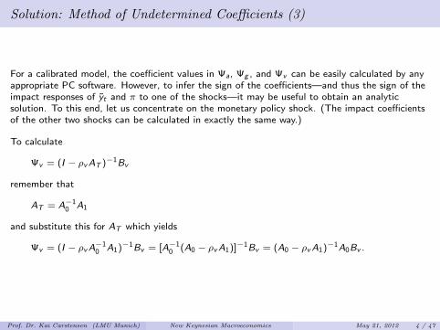
Solution: Method of Undetermined Coefficients (3)
For a calibrated model, the coefficient values in Ψa, Ψg , and Ψv can be easily calculated by anyappropriate PC software. However, to infer the sign of the coefficients—and thus the sign of theimpact responses of yt and π to one of the shocks—it may be useful to obtain an analyticsolution. To this end, let us concentrate on the monetary policy shock. (The impact coefficientsof the other two shocks can be calculated in exactly the same way.)
To calculate
Ψv = (I − ρvAT )−1Bv
remember that
AT = A−10 A1
and substitute this for AT which yields
Ψv = (I − ρvA−10 A1)−1Bv = [A−1
0 (A0 − ρvA1)]−1Bv = (A0 − ρvA1)−1A0Bv .
Prof. Dr. Kai Carstensen (LMU Munich) New Keynesian Macroeconomics May 21, 2012 4 / 47
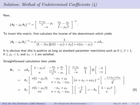
Solution: Method of Undetermined Coefficients (4)
Now,
(A0 − ρvA1)−1 =
[ σ+φy
σ− ρv φπ
σ− ρv
σ−κ 1− ρvβ
]−1
.
To invert this matrix, first calculate the inverse of the determinant which yields
|A0 − ρvA1|−1 = σ1
(1− βρv )[σ(1− ρv ) + φy ] + κ(φπ − ρv )= σΛv .
It is obvious that this is positive as long as standard parameter restrictions such as 0 ≤ β < 1,0 ≤ ρv < 1, and φπ > 1 are satisfied.
Straightforward calculation then yields
Ψv = σΛv
[1− ρvβ −φπ
σ+ ρv
σ
κσ+φy
σ− ρv
] [ σ+φy
σφπσ
−κ 1
]Ω
[−1−κ
]
= Λv
[σ(1− ρvβ) −φπ + ρv
σκ σ + φy − σρv
](σ + φy + κφπ)−1
[−σ+φy +κφπ
σ0
]= Λv
[σ(1− ρvβ) −φπ + ρv
σκ σ + φy − σρv
] [− 1σ
0
]= −Λv
[1− ρvβ
κ
]. (8)
Prof. Dr. Kai Carstensen (LMU Munich) New Keynesian Macroeconomics May 21, 2012 5 / 47

Solution: Method of Undetermined Coefficients (5)
By the same method, one obtains for the impact coefficients of the technology shock as
Ψa = (A0 − ρaA1)−1A0Ba
with
|A0 − ρaA1|−1 = σ1
(1− βρa)[σ(1− ρa) + φy ] + κ(φπ − ρa)= σΛa,
which is again positive.
Straightforward calculation then yields
Ψa = σΛa
[1− ρaβ −φπ
σ+ ρa
σ
κσ+φy
σ− ρa
] [ σ+φy
σφπσ
−κ 1
]Ω
[− (1+ϕ)(1−ρa)
ω0
]= −Λaσ(1− ρa)ψn
ya
[1− ρaβ
κ
](9)
where
ψnya =
1 + ϕ
α+ ϕ+ σ(1− α)=
1 + ϕ
ω> 0
is the impact coefficient of at on ynt .
Prof. Dr. Kai Carstensen (LMU Munich) New Keynesian Macroeconomics May 21, 2012 6 / 47

Solution: Method of Undetermined Coefficients (6)
Finally, one obtains for the impact coefficients of the government demand shock as
Ψg = (A0 − ρgA1)−1A0Bg
with
|A0 − ρgA1|−1 = σ1
(1− βρg )[σ(1− ρg ) + φy ] + κ(φπ − ρg )= σΛg ,
which is again positive.
Straightforward calculation then yields
Ψg = σΛg
[1− ρgβ −φπ
σ+ρgσ
κσ+φy
σ− ρg
][ σ+φy
σφπσ
−κ 1
]Ω
[− (α+ϕ)(1−ρg )
ω0
]
= Λgσ(1− ρg )(1− ψnyg )
[1− ρgβ
κ
](10)
where
ψnyg =
σ(1− α)
ω= 1−
α+ ϕ
ω> 0
is the impact coefficient of gt on ynt .
Prof. Dr. Kai Carstensen (LMU Munich) New Keynesian Macroeconomics May 21, 2012 7 / 47

Solution: Method of Undetermined Coefficients (7)
Now that Ψa, Ψg , and Ψv are known, the dynamic reactions of yt and πt to one of the threeshocks can be traced out using
zt = Ψaat + Ψggt + Ψvvt .
From this the reactions of all remaining variables can be inferred using the other model equations.For example, the reaction of it to a monetary policy shock (shutting down all other shocks) is
it = ρ+ φππt + φy yt + vt
= ρ+ [−φπκΛv − φy (1− βρv )Λv + 1] vt
= ρ+[−φπκ− φy (1− βρv ) + Λ−1
v
]Λvvt
= ρ+ [−φπκ− φy (1− βρv ) + (1− βρv )[σ(1− ρv ) + φy ] + κ(φπ − ρv )] Λvvt
= ρ+ [(1− βρv )(1− ρv )σ + ρvκ] Λvvt .
Prof. Dr. Kai Carstensen (LMU Munich) New Keynesian Macroeconomics May 21, 2012 8 / 47

Part 11: The Blanchard-Kahn Solution Method
Prof. Dr. Kai Carstensen (LMU Munich) New Keynesian Macroeconomics May 21, 2012 9 / 47

The Blanchard-Kahn Approach
The Blanchard-Kahn approach to solve DSGE model is an alternative to the method ofundetermined coefficients. In standard models such as the new Keynesian baseline model they areequally appropriate and lead to the same stable solution.
The Blanchard-Kahn approach requires that the DSGE-model be expressed as system ofdifference equations of order 1 in matrix form. Specifically, it is written in the form
F0
(X1,t+1
EtX2,t+1
)= F1
(X1,t
X2,t
)+ G0εt+1.
It is assumed that there exist n1 predetermined variables X1,t and n2 jump variables X2,t .
To be applicable, the Blanchard-Kahn approach requires stationary, zero-mean variables. To thisend, typically all variables are defined as deviations from the non-stochastic steady state.
In addition, the model needs to be reduced such that the coefficient matrix A0 is invertible.
In this course, we will not study the full Blanchard-Kahn algorithm but only the appropriatematrix form and the related stability condition. This will help to interpret the output of theDynare package.
Prof. Dr. Kai Carstensen (LMU Munich) New Keynesian Macroeconomics May 21, 2012 10 / 47
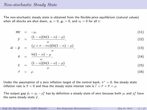
Non-stochastic Steady State
The non-stochastic steady state is obtained from the flexible-price equilibrium (natural values)when all shocks are shut down, at = 0, gt = 0, and vt = 0 for all t:
mc = −µ, (11)
y =(1− α)(ln(1− α)− µ)
ω, (12)
w − p =(ϕ+ σ − σα)(ln(1− α)− µ)
ω, (13)
n =ln(1− α)− µ
ω, (14)
c =(1− α)(ln(1− α)− µ)
ω, (15)
r = ρ. (16)
Under the assumption of a zero inflation target of the central bank, π∗ = 0, the steady stateinflation rate is π = 0 and thus the steady state interest rate is i = r + π = ρ.
The output gap yt = yt − ynt has by definition a steady state of zero because both yt and yn
t havethe same steady state y .
Prof. Dr. Kai Carstensen (LMU Munich) New Keynesian Macroeconomics May 21, 2012 11 / 47
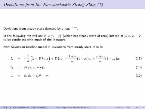
Deviations from the Non-stochastic Steady State (1)
Deviations from steady state denoted by a hat: “ˆ”.
In the following, we will use yt = yt − ynt (which has steady state of zero) instead of yt = yt − y
to be consistent with much of the literature.
New Keynesian baseline model in deviations from steady state then is:
yt = −1
σ
(it − Et πt+1
)+ Et yt+1 −
1 + ϕ
ω(1− ρa)at +
ϕ+ α
ω(1− ρg )gt (17)
πt = βEt πt+1 + κyt (18)
it = φππt + φy yt + vt (19)
Prof. Dr. Kai Carstensen (LMU Munich) New Keynesian Macroeconomics May 21, 2012 12 / 47
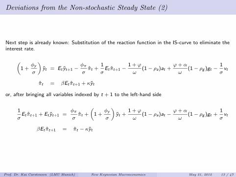
Deviations from the Non-stochastic Steady State (2)
Next step is already known: Substitution of the reaction function in the IS-curve to eliminate theinterest rate.
(1 +
φy
σ
)yt = Et yt+1 −
φπ
σπt +
1
σEt πt+1 −
1 + ϕ
ω(1− ρa)at +
ϕ+ α
ω(1− ρg )gt −
1
σvt
πt = βEt πt+1 + κyt
or, after bringing all variables indexed by t + 1 to the left-hand side
1
σEt πt+1 + Et yt+1 =
φπ
σπt +
(1 +
φy
σ
)yt +
1 + ϕ
ω(1− ρa)at −
ϕ+ α
ω(1− ρg )gt +
1
σvt
βEt πt+1 = πt − κyt
Prof. Dr. Kai Carstensen (LMU Munich) New Keynesian Macroeconomics May 21, 2012 13 / 47

Exogenous Shock Processes
The exogenous shock processes have to be added to the model because the disturbance term inthe Blanchard-Kahn matrix form needs to be white noise:
vt+1 = ρvvt + εvt+1
at+1 = ρaat + εat+1
gt+1 = ρggt + εgt+1
The shock processes are predetermined in the sense that they depend on their past realizationsbut not on expected future variables.
Prof. Dr. Kai Carstensen (LMU Munich) New Keynesian Macroeconomics May 21, 2012 14 / 47
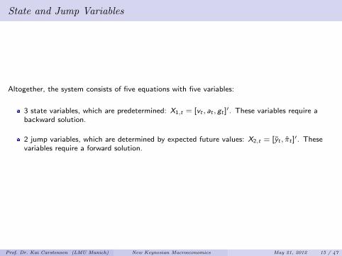
State and Jump Variables
Altogether, the system consists of five equations with five variables:
3 state variables, which are predetermined: X1,t = [vt , at , gt ]′. These variables require abackward solution.
2 jump variables, which are determined by expected future values: X2,t = [yt , πt ]′. Thesevariables require a forward solution.
Prof. Dr. Kai Carstensen (LMU Munich) New Keynesian Macroeconomics May 21, 2012 15 / 47

Matrix Form (1)
1 0 0 0 00 1 0 0 00 0 1 0 00 0 0 1
σ1
0 0 0 β 0
︸ ︷︷ ︸
F0
at+1
gt+1
vt+1
Et πt+1
Et yt+1
=
ρa 0 0 0 00 ρg 0 0 00 0 ρv 0 0
(1+ϕ)(1−ρa)ω
− (ϕ+α)(1−ρg )
ω1σ
φπσ
σ+φy
σ0 0 0 1 −κ
︸ ︷︷ ︸
F1
atgtvtπtyt
+
1 0 00 1 00 0 10 0 00 0 0
︸ ︷︷ ︸
G0
εat+1εgt+1εvt+1
Prof. Dr. Kai Carstensen (LMU Munich) New Keynesian Macroeconomics May 21, 2012 16 / 47

Matrix Form (2)
To solve the system
F0
(X1,t+1
EtX2,t+1
)= F1
(X1,t
X2,t
)+ G0εt+1
we first have to bring F0 to the right-hand side which yields(X1,t+1
EtX2,t+1
)= F−1
0 F1︸ ︷︷ ︸=F
(X1,t
X2,t
)+ F−1
0 G0︸ ︷︷ ︸=G
εt+1,
or, in short,
EtXt+1 = F Xt + Gεt+1.
Prof. Dr. Kai Carstensen (LMU Munich) New Keynesian Macroeconomics May 21, 2012 17 / 47
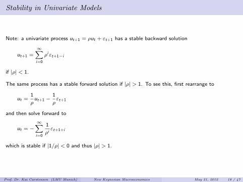
Stability in Univariate Models
Note: a univariate process ut+1 = ρut + εt+1 has a stable backward solution
ut+1 =∞∑i=0
ρiεt+1−i
if |ρ| < 1.
The same process has a stable forward solution if |ρ| > 1. To see this, first rearrange to
ut =1
ρut+1 −
1
ρεt+1
and then solve forward to
ut = −∞∑i=0
1
ρiεt+1+i
which is stable if |1/ρ| < 0 and thus |ρ| > 1.
Prof. Dr. Kai Carstensen (LMU Munich) New Keynesian Macroeconomics May 21, 2012 18 / 47
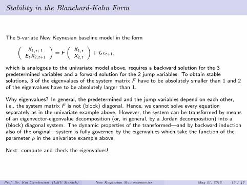
Stability in the Blanchard-Kahn Form
The 5-variate New Keynesian baseline model in the form(X1,t+1
EtX2,t+1
)= F
(X1,t
X2,t
)+ Gεt+1,
which is analogous to the univariate model above, requires a backward solution for the 3predetermined variables and a forward solution for the 2 jump variables. To obtain stablesolutions, 3 of the eigenvalues of the system matrix F have to be absolutely smaller than 1 and 2of the eigenvalues have to be absolutely larger than 1.
Why eigenvalues? In general, the predetermined and the jump variables depend on each other,i.e., the system matrix F is not (block) diagonal. Hence, we cannot solve every equationseparately as in the univariate example above. However, the system can be transformed by meansof an eigenvector-eigenvalue decomposition (or, in general, by a Jordan decomposition) into a(block) diagonal system. The dynamic properties of the transformed—and by backward inductionalso of the original—system is fully governed by the eigenvalues which take the function of theparameter ρ in the univariate example above.
Next: compute and check the eigenvalues!
Prof. Dr. Kai Carstensen (LMU Munich) New Keynesian Macroeconomics May 21, 2012 19 / 47
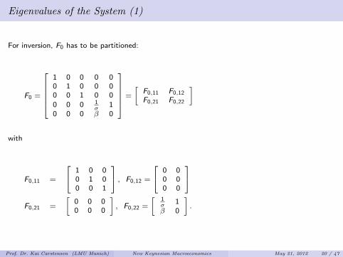
Eigenvalues of the System (1)
For inversion, F0 has to be partitioned:
F0 =
1 0 0 0 00 1 0 0 00 0 1 0 00 0 0 1
σ1
0 0 0 β 0
=
[F0,11 F0,12
F0,21 F0,22
]
with
F0,11 =
1 0 00 1 00 0 1
, F0,12 =
0 00 00 0
F0,21 =
[0 0 00 0 0
], F0,22 =
[1σ
1β 0
].
Prof. Dr. Kai Carstensen (LMU Munich) New Keynesian Macroeconomics May 21, 2012 20 / 47

Eigenvalues of the System (2)
Inversion of the diagonal matrices yields
F−10,11 =
1 0 00 1 00 0 1
, F−10,22 =
[0 1/β1 −1/(βσ)
].
Block diagonal structure: inversion of F0 by inversion of the diagonal matrices
F−10 =
1 0 0 0 00 1 0 0 00 0 1 0 00 0 0 0 1/β0 0 0 1 −1/(βσ)
.
Prof. Dr. Kai Carstensen (LMU Munich) New Keynesian Macroeconomics May 21, 2012 21 / 47
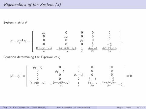
Eigenvalues of the System (3)
System matrix F
F = F−10 F1 =
ρa 0 0 0 00 ρg 0 0 00 0 ρv 0 00 0 0 1
β−κβ
(1+ϕ)(1−ρa)ω
− (α+ϕ)(1−ρg )
ω1σ
βφπ−1βσ
βσ+βφy +κ
βσ
.
Equation determining the Eigenvalues ξ
|A− ξI | =
∣∣∣∣∣∣∣∣∣∣∣
ρa − ξ 0 0 0 00 ρg − ξ 0 0 00 0 ρv − ξ 0 00 0 0 1
β− ξ −κ
β(1+ϕ)(1−ρa)
ω− (α+ϕ)(1−ρg )
ω1σ
βφπ−1βσ
βσ+βφy +κ
βσ− ξ
∣∣∣∣∣∣∣∣∣∣∣= 0.
Prof. Dr. Kai Carstensen (LMU Munich) New Keynesian Macroeconomics May 21, 2012 22 / 47
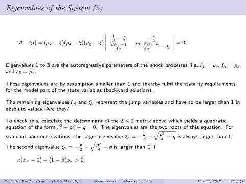
Eigenvalues of the System (5)
|A− ξI | = (ρv − ξ)(ρa − ξ)(ρg − ξ)
∣∣∣∣∣1β− ξ −κ
ββφπ−1βσ
βσ+βφy +κ
βσ− ξ
∣∣∣∣∣ = 0.
Eigenvalues 1 to 3 are the autoregressive parameters of the shock processes, i.e. ξ1 = ρa, ξ2 = ρgand ξ3 = ρv .
These eigenvalues are by assumption smaller than 1 and thereby fulfil the stability requirementsfor the model part of the state variables (backward solution).
The remaining eigenvalues ξ4 and ξ5 represent the jump variables and have to be larger than 1 inabsolute values. Are they?
To check this, calculate the determinant of the 2× 2 matrix above which yields a quadraticequation of the form ξ2 + pξ + q = 0. The eigenvalues are the two roots of this equation. For
standard parameterizations, the larger eigenvalue ξ4 = − p2
+√
p2
4− q is always larger than 1.
The second eigenvalue ξ5 = − p2−√
p2
4− q is larger than 1 if
κ(φπ − 1) + (1− β)φy > 0.
Prof. Dr. Kai Carstensen (LMU Munich) New Keynesian Macroeconomics May 21, 2012 23 / 47

Interpretation of the Stability Condition
Write the stability condition as
φπ +1− βκ
φy > 1.
Now consider the case of a persistent increase in inflation: d πt = Etd πt+1 = dπ > 0.
According to the Phillips curve, this leads to an increase in the output gap:
dπ = βEtdπ + κdyt ⇒ dyt = 1−βκ
dπ
The central bank follows its reaction function:
dit = φπd πt + φydyt = φπdπ + φy1−βκ
dπ =(φπ + φy
1−βκ
)dπ.
To satisfy the requirement dit > d π such that drt > 0 (Taylor principle), the condition
φπ + φy1−βκ
> 1 has to hold.
More clearly: if the central bank only reacts to inflation (φy = 0), then the condition is reducedto φπ > 1.
Prof. Dr. Kai Carstensen (LMU Munich) New Keynesian Macroeconomics May 21, 2012 24 / 47

The Blanchard-Kahn Algorithm
Once stability is confirmed, the DSGE model(X1,t+1
EtX2,t+1
)= F
(X1,t
X2,t
)+ Gεt+1
can be solved by the Blanchard-Kahn algorithm which is an iterative procedure. Typically, this isdone by software packages such as Dynare.
Due to time constraints, we will not do it in the lecture.
Prof. Dr. Kai Carstensen (LMU Munich) New Keynesian Macroeconomics May 21, 2012 25 / 47

Part 12: Allocation Distortions in the New Keynesian Model
Prof. Dr. Kai Carstensen (LMU Munich) New Keynesian Macroeconomics May 21, 2012 26 / 47

State Dependent Allocation Distortions (1)
To understand the model and to correctly interpret the reaction to one of the shocks, it isimportant to observe the allocation distortions in the new Keynesian baseline model:
Different to the RBC model, the allocation distortions in the New Keynesian model implythat resource allocation is inefficient.
In equilibrium, the market power of the companies leads to suboptimal high prices andsuboptimal low production.
After exogenous shocks, the existence of staggered price adjustment prevents that the steadystate will be reached immediately. This implies that also the allocation distortion is notconstant bur fluctuating.
Without subsidies that compensate for the distortion (see Gali, p. 73), expansionary demandshocks can be advantageous on the macroeconomic level because they push productiontowards the efficient level.
Prof. Dr. Kai Carstensen (LMU Munich) New Keynesian Macroeconomics May 21, 2012 27 / 47

State Dependent Allocation Distortions (2)
Efficient allocation:
The demand is the same for all consumption goods: Ct(i) = Ct ∀ i ∈ [0, 1].
The level of labor is identical for all firms: Nt(i) = Nt ∀ i ∈ [0, 1].
Reason: consumption goods affect the utility function symmetrically. All firms have the sameproduction technology.
On average – and from this also for every good – the marginal rate of substitution betweenleisure time F and consumption C should be equal to the marginal product of labor, i.e.
∂U/∂Ft
∂U/∂Ct= −
∂U/∂Nt
∂U/∂Ct︸ ︷︷ ︸MRSt
=Wt
Pt=∂Yt
∂Nt︸ ︷︷ ︸MPNt
.
The households can adjust their marginal utility flexibly to the real wage Wt/Pt , such thatMRSt = Wt/Pt holds at every point of time.
Prof. Dr. Kai Carstensen (LMU Munich) New Keynesian Macroeconomics May 21, 2012 28 / 47
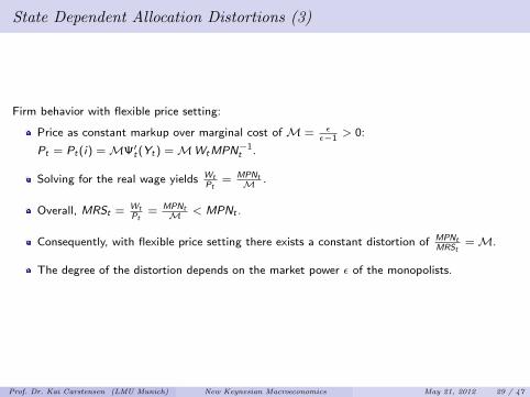
State Dependent Allocation Distortions (3)
Firm behavior with flexible price setting:
Price as constant markup over marginal cost of M = εε−1
> 0:
Pt = Pt(i) =MΨ′t(Yt) =MWtMPN−1t .
Solving for the real wage yields WtPt
= MPNtM .
Overall, MRSt = WtPt
= MPNtM < MPNt .
Consequently, with flexible price setting there exists a constant distortion of MPNtMRSt
=M.
The degree of the distortion depends on the market power ε of the monopolists.
Prof. Dr. Kai Carstensen (LMU Munich) New Keynesian Macroeconomics May 21, 2012 29 / 47

State Dependent Allocation Distortions (4)
Firm behavior with staggered price setting:
Optimal price is chosen as markup over current and expected marginal costs. Price level isweighted average of optimal price (chosen by the adjusting firms) and the previous price level(charged by the non-adjusting firms). Hence, after a shock the markup will generallyfluctuate over time and differ from the flexible-price markup M.
Define the average sticky price markup as Mt = PtΨ′t
= Pt
WtMPN−1t
. Hence, we have
WtPt
= MPNtMt
.
The economy-wide distortion is now MRSt = WtPt
= MPNtMt
.
Note that a shock that reduces the average markup such that Mt <M improves theallocation and thus brings the economy towards the efficient level (unless the shock is largeenough for production to strongly overshoot the efficient level, but this is ruled out by thestandard assumption that shocks are small).
Monetary policy may nevertheless be interested to stabilize Mt at M if, e.g., fiscal policyeliminates the flexible price distortion—more on this later, when optimal monetary policy isdiscussed.
Prof. Dr. Kai Carstensen (LMU Munich) New Keynesian Macroeconomics May 21, 2012 30 / 47

State Dependent Allocation Distortions (5)
For the moment, we will leave the model as it is and simply track the response of our measure ofinefficiency to an exogenous shock. This is informative because it shows whether a shock canimprove the allocation and thereby increase utility. To this end, let us define
µt = lnMt = mpnt − (wt − pt) = yt − nt − (wt − pt) + ln(1− α)
The steady state clearly is
µ = y − n − (w − p) + ln(1− α).
Hence, we have
µt = yt − nt − (wt − pt).
The lower µt the smaller is the distortion and the more efficient is the allocation.
Prof. Dr. Kai Carstensen (LMU Munich) New Keynesian Macroeconomics May 21, 2012 31 / 47

Part 13: Calibration
Prof. Dr. Kai Carstensen (LMU Munich) New Keynesian Macroeconomics May 21, 2012 32 / 47

Calibration (1)
β = 0.99, i.e. the individual time preference rate is ρ = − lnβ ≈ 0.01. As the model issupposed to be calibrated for quarterly data, this implies an annualized time preference rateand real interest rate of about 4%.
σ = ϕ = 1, i.e. the utility function is logarithmic in the level of consumption and quadraticin labor.
ε = 6, i.e. in the case of flexible prices the mark-up of the firms is 20% of the nominalmarginal costs, as M = ε
ε−1= 1.2. Note that µ = ln 1.2 ≈ 0.18 which is slightly less due to
the approximation error.
θ = 2/3, i.e. two third of the prices are fixed in each period. Only one third can be adjusted.
α = 1/3, which is commonly found in the RBC literature and empirically well founded (notethat in a constant returns to scale production function with capital and labor, α = 1/3implies a labor share of 2/3).
Prof. Dr. Kai Carstensen (LMU Munich) New Keynesian Macroeconomics May 21, 2012 33 / 47

Calibration (2)
From this follows λ = 0.0425 and κ = 0.1275. The slope of the Phillips curve, i.e. thesensitivity of the inflation with respect to the output gap, is consequently 0.1275.
φπ = 1.5 and φy = 0.5/4. These are the coefficients as reported by Taylor (1999) for theUnited States. (Division by 4 at φy reflects that we deal here with quarterly data. Incontrast, Taylor deals with annual interest and inflation rates.)
ρv = 0.5, i.e. the monetary policy shock is only moderately persistent.
ρa = ρg = 0.9, i.e. the technology shock and the demand shock possess the same persistencywe assumed in the RBC model.
Prof. Dr. Kai Carstensen (LMU Munich) New Keynesian Macroeconomics May 21, 2012 34 / 47

Calibration of the Shocks
Monetary policy shock: εv1 = −0.25, εvt = 0 ∀ t > 1
Technology shock: εa1 = 1, εat = 0 ∀ t > 1
Public demand shock: εg1 = 0.75, εgt = 0 ∀ t > 1
Prof. Dr. Kai Carstensen (LMU Munich) New Keynesian Macroeconomics May 21, 2012 35 / 47

Part 14: The Effects of a Monetary Policy Shock
Prof. Dr. Kai Carstensen (LMU Munich) New Keynesian Macroeconomics May 21, 2012 36 / 47
The Effects of a Monetary Policy Shock (1)
Concentrating on monetary policy shocks only and hence shutting down all other shocks yieldsthe solution
yt = −Λv (1− ρvβ)vt (20)
πt = −Λvκvt (21)
Since Λv > 0, 1− ρvβ > 0 and κ > 0 as shown above, a contractionary monetary policy shockleads on impact to a decline in both the output gap and the inflation rate.
In the following, we show the impulse responses after an on-off shock in period t = 0 of sizev0 = 0.25. This means that monetary policy unexpectedly increases the interest rate by 25 basispoints. Ceteris paribus, this implies that the annualized nominal interest rate response in period 0shown below is 4× 25 = 100 basis points. However, the central bank realizes that the shockbrings down inflation and the output gap below their targets and immediately reacts to thisendogenously (via the reaction function) by softening monetary policy again. The total impacteffect on the annualized nominal interest rate is slightly below 50 percentage points.
Prof. Dr. Kai Carstensen (LMU Munich) New Keynesian Macroeconomics May 21, 2012 37 / 47

Contractionary Monetary Policy Shock: Impulse Responses (1)
0 2 4 6 8 10 12−0.4
−0.3
−0.2
−0.1
0Output gap yt
0 2 4 6 8 10 12−0.4
−0.3
−0.2
−0.1
0Inflation πt (annualized)
0 2 4 6 8 10 120
0.5
1Annualized rates it (blue) and rt (red)
0 2 4 6 8 10 12−0.4
−0.3
−0.2
−0.1
0Consumption ct
0 2 4 6 8 10 12−1
−0.5
0Labor nt
0 2 4 6 8 10 120
0.1
0.2
0.3
0.4Monetary policy shock vt
Prof. Dr. Kai Carstensen (LMU Munich) New Keynesian Macroeconomics May 21, 2012 38 / 47

Contractionary Monetary Policy Shock: Impulse Responses (2)
0 2 4 6 8 10 12−0.5
−0.4
−0.3
−0.2
−0.1Output yt (blue) and ynt (red)
0 2 4 6 8 10 12−0.4
−0.3
−0.2
−0.1
0Gaps yt (blue) and yt (red)
0 2 4 6 8 10 12−0.8
−0.6
−0.4
−0.2
0
0.2mrst = wt − pt (blue) and mpnt (red)
0 2 4 6 8 10 120
0.2
0.4
0.6
0.8
1Distortion µt
Prof. Dr. Kai Carstensen (LMU Munich) New Keynesian Macroeconomics May 21, 2012 39 / 47

Part 15: The Effects of a Government Demand Shock
Prof. Dr. Kai Carstensen (LMU Munich) New Keynesian Macroeconomics May 21, 2012 40 / 47

Expansionary Government Demand Shock: Impulse Responses (1)
0 10 20 300
0.05
0.1Output gap yt
0 10 20 300
0.1
0.2
0.3
0.4Inflation πt (annualized)
0 10 20 300
0.5
1Annualized rates it (blue) and rt (red)
0 10 20 30−1
−0.5
0Consumption ct
0 10 20 300
0.5
1Labor nt
0 10 20 300
0.5
1Government demand shock gt
Prof. Dr. Kai Carstensen (LMU Munich) New Keynesian Macroeconomics May 21, 2012 41 / 47
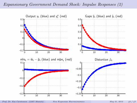
Expansionary Government Demand Shock: Impulse Responses (2)
0 10 20 30−0.2
−0.1
0
0.1
0.2
0.3Output yt (blue) and ynt (red)
0 10 20 300
0.1
0.2
0.3
0.4
0.5Gaps yt (blue) and yt (red)
0 10 20 30−0.3
−0.2
−0.1
0
0.1mrst = wt − pt (blue) and mpnt (red)
0 10 20 30−0.25
−0.2
−0.15
−0.1
−0.05
0Distortion µt
Prof. Dr. Kai Carstensen (LMU Munich) New Keynesian Macroeconomics May 21, 2012 42 / 47

Part 16: The Effects of a Technology Shock
Prof. Dr. Kai Carstensen (LMU Munich) New Keynesian Macroeconomics May 21, 2012 43 / 47
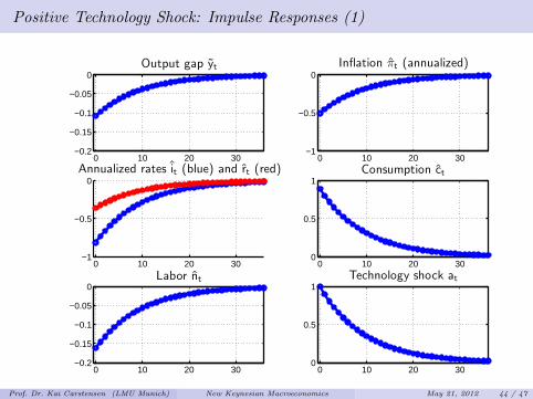
Positive Technology Shock: Impulse Responses (1)
0 10 20 30−0.2
−0.15
−0.1
−0.05
0Output gap yt
0 10 20 30−1
−0.5
0Inflation πt (annualized)
0 10 20 30−1
−0.5
0Annualized rates it (blue) and rt (red)
0 10 20 300
0.5
1Consumption ct
0 10 20 30−0.2
−0.15
−0.1
−0.05
0Labor nt
0 10 20 300
0.5
1Technology shock at
Prof. Dr. Kai Carstensen (LMU Munich) New Keynesian Macroeconomics May 21, 2012 44 / 47
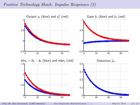
Positive Technology Shock: Impulse Responses (2)
0 10 20 30−0.5
0
0.5
1Output yt (blue) and ynt (red)
0 10 20 30−0.5
0
0.5
1Gaps yt (blue) and yt (red)
0 10 20 300
0.5
1
1.5mrst = wt − pt (blue) and mpnt (red)
0 10 20 300
0.1
0.2
0.3
0.4Distortion µt
Prof. Dr. Kai Carstensen (LMU Munich) New Keynesian Macroeconomics May 21, 2012 45 / 47

Part 17: Critique of the New Keynesian (Baseline-) Model
Prof. Dr. Kai Carstensen (LMU Munich) New Keynesian Macroeconomics May 21, 2012 46 / 47

Critique of the New Keynesian (Baseline-) Model
Are households and firms really as forward-looking and rational? Empirically: autocorrelatedforecast errors.
Calvo price setting cannot match all micro facts: menu costs?
Inflation rate is jump variable! Empirically: inflation seems to be very persistent.
Labour market is in equilibrium! Empirically: high unemployment rate.
Capital accumulation is excluded! Empirically: investments have huge business cycles.
These are only a few extensions of the baseline model.
Prof. Dr. Kai Carstensen (LMU Munich) New Keynesian Macroeconomics May 21, 2012 47 / 47