new facts in finance - booth school of business36 economic perspectives new facts in finance john h....

36 Economic Perspectives

New facts in finance

John H. Cochrane

John H. Cochrane is the Sigmund E. EdelstoneProfessor of Finance in the Graduate School ofBusiness at the University of Chicago, a consultant tothe Federal Reserve Bank of Chicago, and a researchassociate at the National Bureau of Economic Research(NBER). The author thanks Andrea Eisfeldt for researchassistance and David Marshall, John Campbell, andRobert Shiller for comments. The author�s research issupported by the Graduate School of Business and bya grant from the National Science Foundation,administered by the NBER.

Introduction and summary

The last 15 years have seen a revolution in the wayfinancial economists understand the investment world.We once thought that stock and bond returns wereessentially unpredictable. Now we recognize thatstock and bond returns have a substantial predictablecomponent at long horizons. We once thought thatthe capital asset pricing model (CAPM) provided agood description of why average returns on somestocks, portfolios, funds, or strategies were higher thanothers. Now we recognize that the average returns ofmany investment opportunities cannot be explainedby the CAPM, and �multifactor models� are used inits place. We once thought that long-term interestrates reflected expectations of future short-term ratesand that interest rate differentials across countriesreflected expectations of exchange rate depreciation.Now, we see time-varying risk premiums in bond andforeign exchange markets as well as in stock markets.We once thought that mutual fund average returnswere well explained by the CAPM. Now, we see thatfunds can earn average returns not explained by theCAPM, that is, unrelated to market risks, by followinga variety of investment �styles.�

In this article, I survey these new facts, and I showhow they are variations on a common theme. Eachcase uses price variables to infer market expectationsof future returns; each case notices that an offsettingadjustment (to dividends, interest rates, or exchangerates) seems to be absent or sluggish. Each case sug-gests that financial markets offer rewards in the formof average returns for holding risks related to reces-sions and financial distress, in addition to the risksrepresented by overall market movements. In a com-panion article in this issue, �Portfolio advice for a mul-tifactor world,� I survey and interpret recent advancesin portfolio theory that address the question, Whatshould an investor do about all these new facts?

First, a slightly more detailed overview of thefacts then and now. Until the mid-1980s, financial

economists� view of the investment world was basedon three bedrocks:

1. The CAPM is a good measure of risk and thusa good explanation of the fact that some assets (stocks,portfolios, strategies, or mutual funds) earn higheraverage returns than others. The CAPM states thatassets can only earn a high average return if theyhave a high �beta,� which measures the tendencyof the individual asset to move up or down with themarket as a whole. Beta drives average returns becausebeta measures how much adding a bit of the asset toa diversified portfolio increases the volatility of theportfolio. Investors care about portfolio returns, notabout the behavior of specific assets.

2. Returns are unpredictable, like a coin flip. Thisis the random walk theory of stock prices. Thoughthere are bull and bear markets; long sequences ofgood and bad past returns; the expected future returnis always about the same. Technical analysis thattries to divine future returns from patterns of pastreturns and prices is nearly useless. Any apparentpredictability is either a statistical artifact which willquickly vanish out of sample or cannot be exploitedafter transaction costs.

Bond returns are not predictable. This is theexpectations model of the term structure. If long-termbond yields are higher than short-term yields�if theyield curve is upward sloping�this does not meanthat you expect a higher return by holding long-termbonds rather than short-term bonds. Rather, it means

37Federal Reserve Bank of Chicago

that short-term interest rates are expected to rise inthe future. Over one year, the rise in interest rates willlimit the capital gain on long-term bonds, so they earnthe same as the short-term bonds over the year. Overmany years, the rise in short rates improves the rateof return from rolling over short-term bonds to equalthat of holding the long-term bond. Thus, you expectto earn about the same amount on short-term or long-term bonds at any horizon.

Foreign exchange bets are not predictable. If acountry has higher interest rates than are available inthe U.S. for bonds of a similar risk class, its exchangerate is expected to depreciate. Then, after you con-vert your investment back to dollars, you expect tomake the same amount of money holding foreign ordomestic bonds.

In addition, stock market volatility does notchange much through time. Not only are returns closeto unpredictable, they are nearly identically distributedas well. Each day, the stock market return is like theresult of flipping the same coin, over and over again.

3. Professional managers do not reliably outper-form simple indexes and passive portfolios once onecorrects for risk (beta). While some do better than themarket in any given year, some do worse, and theoutcomes look very much like luck. Funds that do wellin one year are not more likely to do better than aver-age the next year. The average actively managed fundperforms about 1 percent worse than the market index.The more actively a fund trades, the lower the returnsto investors.

Together, these views reflect a guiding principlethat asset markets are, to a good approximation, infor-mationally efficient (Fama, 1970, 1991). Market pricesalready contain most information about fundamentalvalue and, because the business of discovering infor-mation about the value of traded assets is extremelycompetitive, there are no easy quick profits to be made,just as there are not in any other well-establishedand competitive industry. The only way to earn largereturns is by taking on additional risk.

These views are not ideological or doctrinairebeliefs. Rather, they summarize the findings of a quar-ter century of careful empirical work. However, everyone of them has now been extensively revised by anew generation of empirical research. The new find-ings need not overturn the cherished view that marketsare reasonably competitive and, therefore, reasonablyefficient. However, they do substantially enlarge ourview of what activities provide rewards for holdingrisks, and they challenge our understanding of thoserisk premiums.

Now, we know that:1. There are assets whose average returns can

not be explained by their beta. Multifactor extensionsof the CAPM dominate the description, performanceattribution, and explanation of average returns. Mul-tifactor models associate high average returns with atendency to move with other risk factors in additionto movements in the market as a whole. (See box 1.)

2. Returns are predictable. In particular: Variablesincluding the dividend/price (d/p) ratio and term pre-mium can predict substantial amounts of stock returnvariation. This phenomenon occurs over businesscycle and longer horizons. Daily, weekly, and monthlystock returns are still close to unpredictable, and tech-nical systems for predicting such movements are stillclose to useless.

Bond returns are predictable. Though the expec-tations model works well in the long run, a steeplyupward sloping yield curve means that expectedreturns on long-term bonds are higher than on short-term bonds for the next year. These predictions are notguarantees�there is still substantial risk�but thetendency is discernible.

Foreign exchange returns are predictable. If youput your money in a country whose interest rates arehigher than usual relative to the U.S., you expect toearn more money even after converting back to dollars.Again, this prediction is not a guarantee�exchangerates do vary, and a lot, so the strategy is risky.

Volatility does change through time. Times ofpast volatility indicate future volatility. Volatility alsois higher after large price drops. Bond market volatili-ty is higher when interest rates are higher, and possi-bly when interest rate spreads are higher as well.

3. Some mutual funds seem to outperform simpleindexes, even after controlling for risk through marketbetas. Fund returns are also slightly predictable: Pastwinning funds seem to do better than average in thefuture, and past losing funds seem to do worse thanaverage in the future. For a while, this seemed to indi-cate that there is some persistent skill in active man-agement. However, multifactor models explain mostfund persistence: Funds earn persistent returns byfollowing fairly mechanical styles, not by persistentskill at stock selection.

Again, these statements are not dogma, but acautious summary of a large body of careful empiricalwork. The strength and usefulness of many resultsare hotly debated, as are the underlying reasons formany of these new facts. But the old world is gone.


The CAPM and multifactor models

The CAPMThe CAPM proved stunningly successful in a

quarter century of empirical work. Every strategy thatseemed to give high average returns turned out tohave a high beta, or a large tendency to move withthe market. Strategies that one might have thoughtgave high average returns (such as holding very vol-atile stocks) turned out not to have high averagereturns when they did not have high betas.

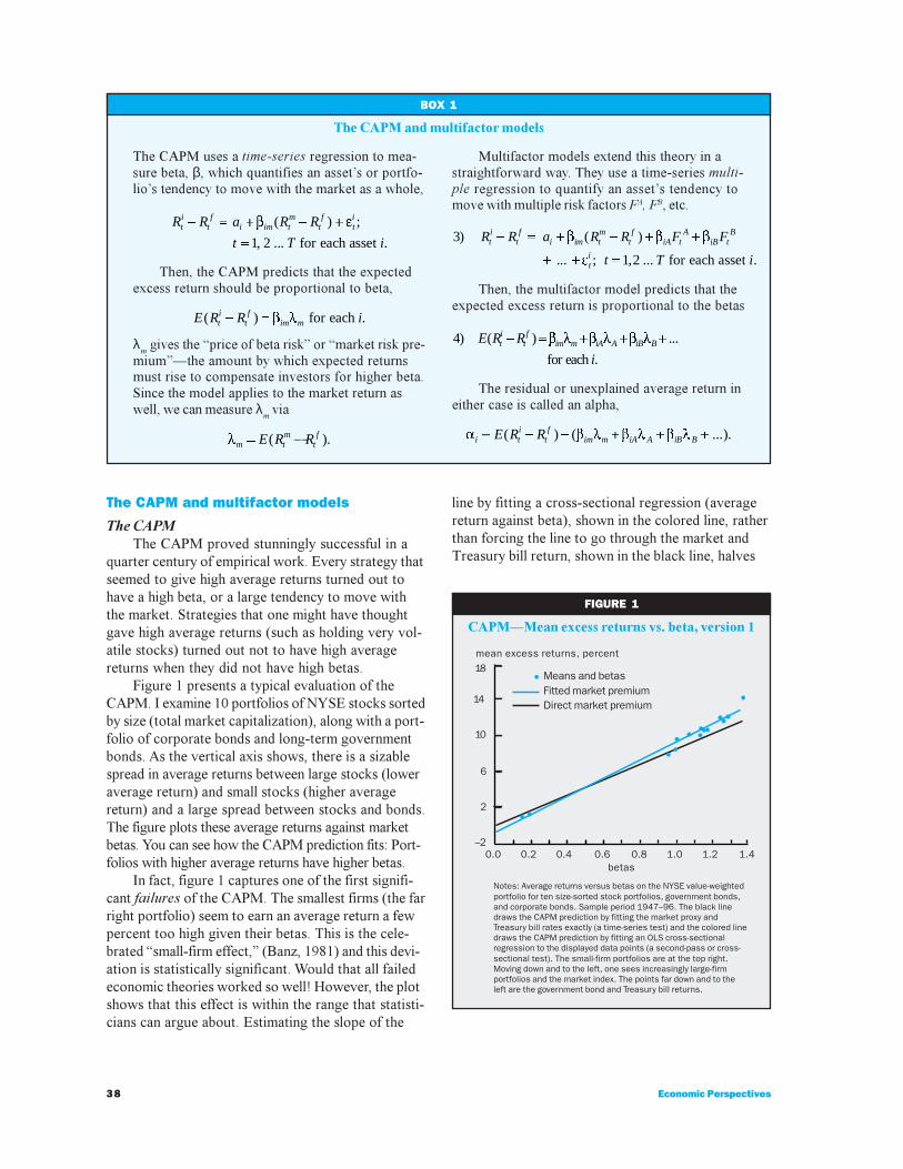
Figure 1 presents a typical evaluation of theCAPM. I examine 10 portfolios of NYSE stocks sortedby size (total market capitalization), along with a port-folio of corporate bonds and long-term governmentbonds. As the vertical axis shows, there is a sizablespread in average returns between large stocks (loweraverage return) and small stocks (higher averagereturn) and a large spread between stocks and bonds.The figure plots these average returns against marketbetas. You can see how the CAPM prediction fits: Port-folios with higher average returns have higher betas.

In fact, figure 1 captures one of the first signifi-cant failures of the CAPM. The smallest firms (the farright portfolio) seem to earn an average return a fewpercent too high given their betas. This is the cele-brated �small-firm effect,� (Banz, 1981) and this devi-ation is statistically significant. Would that all failedeconomic theories worked so well! However, the plotshows that this effect is within the range that statisti-cians can argue about. Estimating the slope of the

line by fitting a cross-sectional regression (averagereturn against beta), shown in the colored line, ratherthan forcing the line to go through the market andTreasury bill return, shown in the black line, halves

BOX 1

The CAPM and multifactor models

The CAPM uses a time-series regression to mea-sure beta, β, which quantifies an asset�s or portfo-lio�s tendency to move with the market as a whole,

R R a R R

t T iti

tf

i im tm

tf

ti- = + - +

=

b e( ) ;

, ... .1 2 for each asset

Then, the CAPM predicts that the expectedexcess return should be proportional to beta,

E R R iti

tf

im m( ) .- = b l for each

λm gives the �price of beta risk� or �market risk pre-

mium��the amount by which expected returnsmust rise to compensate investors for higher beta.Since the model applies to the market return aswell, we can measure λ

m via

lm tm

tfE R R= -( ).

Multifactor models extend this theory in astraightforward way. They use a time-series multi-ple regression to quantify an asset�s tendency tomove with multiple risk factors FA, FB, etc.

3

1 2

) ( )

... ; , ... .

R R a R R F F

t T i

ti

tf

i im tm

tf

iA tA

iB tB

ti

- = + - + +

+ + =

b b b

e for each asset

Then, the multifactor model predicts that theexpected excess return is proportional to the betas

4) ( ) ...

.

E R R

iti

tf

im m iA A iB B- = + + +b l b l b l

for each

The residual or unexplained average return ineither case is called an alpha,

a b l b l b li ti

tf

im m iA A iB BE R R¢ - - + + +( ) ( ...).

FIGURE 1

CAPM�Mean excess returns vs. beta, version 1

mean excess returns, percent

Fitted market premium

Notes: Average returns versus betas on the NYSE value-weightedportfolio for ten size-sorted stock portfolios, government bonds,and corporate bonds. Sample period 1947–96. The black linedraws the CAPM prediction by fitting the market proxy andTreasury bill rates exactly (a time-series test) and the colored linedraws the CAPM prediction by fitting an OLS cross-sectionalregression to the displayed data points (a second-pass or cross-sectional test). The small-firm portfolios are at the top right.Moving down and to the left, one sees increasingly large-firmportfolios and the market index. The points far down and to theleft are the government bond and Treasury bill returns.

Direct market premium

Means and betas18

14

10

6

2

–20.0 0.2 0.4 0.6 0.8 1.0 1.2 1.4

betas


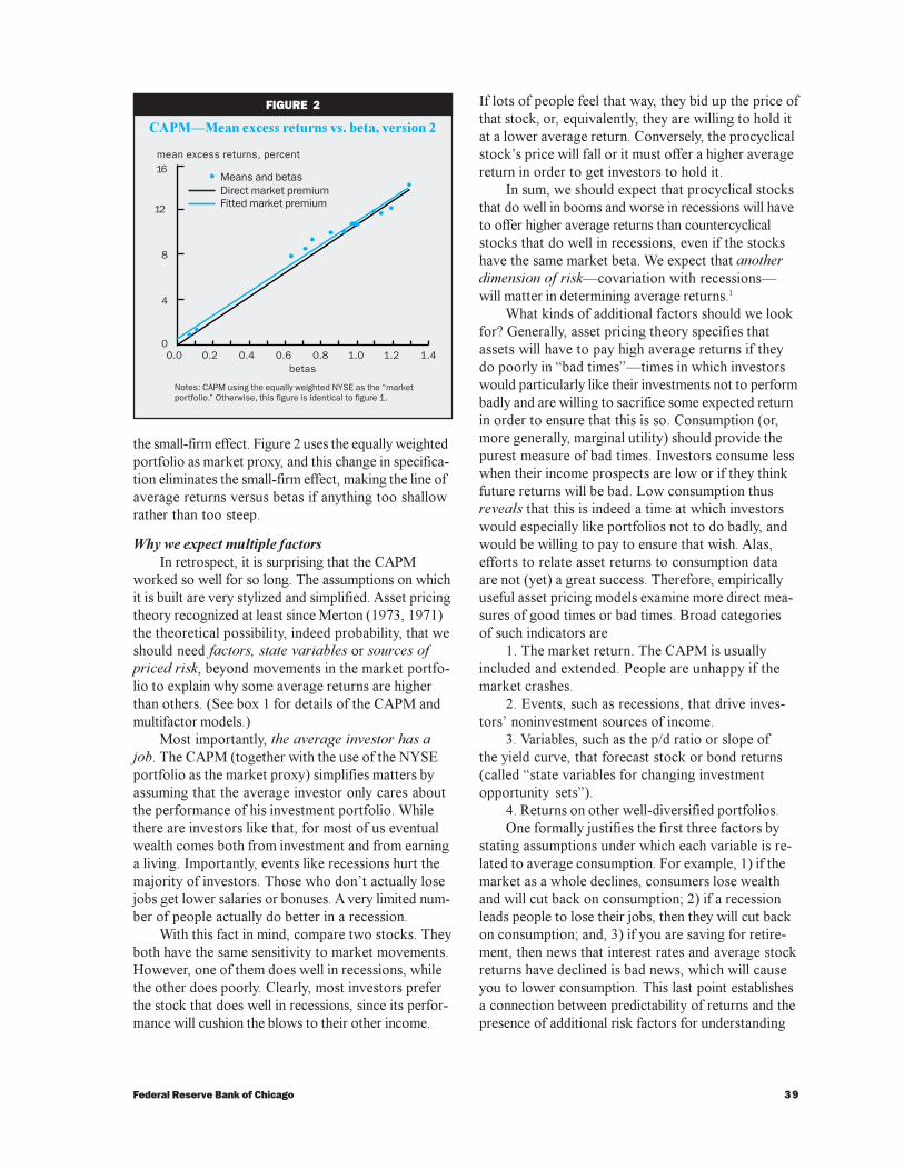
the small-firm effect. Figure 2 uses the equally weightedportfolio as market proxy, and this change in specifica-tion eliminates the small-firm effect, making the line ofaverage returns versus betas if anything too shallowrather than too steep.

Why we expect multiple factorsIn retrospect, it is surprising that the CAPM

worked so well for so long. The assumptions on whichit is built are very stylized and simplified. Asset pricingtheory recognized at least since Merton (1973, 1971)the theoretical possibility, indeed probability, that weshould need factors, state variables or sources ofpriced risk, beyond movements in the market portfo-lio to explain why some average returns are higherthan others. (See box 1 for details of the CAPM andmultifactor models.)

Most importantly, the average investor has ajob. The CAPM (together with the use of the NYSEportfolio as the market proxy) simplifies matters byassuming that the average investor only cares aboutthe performance of his investment portfolio. Whilethere are investors like that, for most of us eventualwealth comes both from investment and from earninga living. Importantly, events like recessions hurt themajority of investors. Those who don�t actually losejobs get lower salaries or bonuses. A very limited num-ber of people actually do better in a recession.

With this fact in mind, compare two stocks. Theyboth have the same sensitivity to market movements.However, one of them does well in recessions, whilethe other does poorly. Clearly, most investors preferthe stock that does well in recessions, since its perfor-mance will cushion the blows to their other income.

If lots of people feel that way, they bid up the price ofthat stock, or, equivalently, they are willing to hold itat a lower average return. Conversely, the procyclicalstock�s price will fall or it must offer a higher averagereturn in order to get investors to hold it.

In sum, we should expect that procyclical stocksthat do well in booms and worse in recessions will haveto offer higher average returns than countercyclicalstocks that do well in recessions, even if the stockshave the same market beta. We expect that anotherdimension of risk�covariation with recessions�will matter in determining average returns.1

What kinds of additional factors should we lookfor? Generally, asset pricing theory specifies thatassets will have to pay high average returns if theydo poorly in �bad times��times in which investorswould particularly like their investments not to performbadly and are willing to sacrifice some expected returnin order to ensure that this is so. Consumption (or,more generally, marginal utility) should provide thepurest measure of bad times. Investors consume lesswhen their income prospects are low or if they thinkfuture returns will be bad. Low consumption thusreveals that this is indeed a time at which investorswould especially like portfolios not to do badly, andwould be willing to pay to ensure that wish. Alas,efforts to relate asset returns to consumption dataare not (yet) a great success. Therefore, empiricallyuseful asset pricing models examine more direct mea-sures of good times or bad times. Broad categoriesof such indicators are

1. The market return. The CAPM is usuallyincluded and extended. People are unhappy if themarket crashes.

2. Events, such as recessions, that drive inves-tors� noninvestment sources of income.

3. Variables, such as the p/d ratio or slope ofthe yield curve, that forecast stock or bond returns(called �state variables for changing investmentopportunity sets�).

4. Returns on other well-diversified portfolios.One formally justifies the first three factors by

stating assumptions under which each variable is re-lated to average consumption. For example, 1) if themarket as a whole declines, consumers lose wealthand will cut back on consumption; 2) if a recessionleads people to lose their jobs, then they will cut backon consumption; and, 3) if you are saving for retire-ment, then news that interest rates and average stockreturns have declined is bad news, which will causeyou to lower consumption. This last point establishesa connection between predictability of returns and thepresence of additional risk factors for understanding

FIGURE 2

CAPM�Mean excess returns vs. beta, version 2

mean excess returns, percent

Direct market premium

Notes: CAPM using the equally weighted NYSE as the “marketportfolio.” Otherwise, this figure is identical to figure 1.

Fitted market premium

Means and betas16

12

8

4

00.0 0.2 0.4 0.6 0.8 1.0 1.2 1.4

betas


the cross-section of average returns. As pointed outby Merton (1971), one would give up some averagereturn to have a portfolio that did well when therewas bad news about future market returns.

The fourth kind of factor�additional portfolioreturns�is most easily defended as a proxy for any ofthe other three. The fitted value of a regression of anypricing factor on the set of all asset returns is a portfo-lio that carries exactly the same pricing information asthe original factor�a factor-mimicking portfolio.

It is vital that the extra risk factors affect theaverage investor. If an event makes investor A worseoff and investor B better off, then investor A buysassets that do well when the event happens and inves-tor B sells them. They transfer the risk of the event,but the price or expected return of the asset is unaf-fected. For a factor to affect prices or expected returns,it must affect the average investor, so investors collec-tively bid up or down the price and expected return ofassets that covary with the event rather than just trans-ferring the risk without affecting equilibrium prices.

Inspired by this broad direction, empirical research-ers have found quite a number of specific factors thatseem to explain the variation in average returns acrossassets. In general, empirical success varies inverselywith theoretical purity.

Small and value/growth stocksThe size and book to market factors advocated

by Fama and French (1996) are one of the most popu-lar additional risk factors.

Small-cap stocks have small market values (pricetimes shares outstanding). Value (or high book/market)stocks have market values that are small relative tothe value of assets on the company�s books. Bothcategories of stocks have quite high average returns.Large and growth stocks are the opposite of smalland value and seem to have unusually low averagereturns. (See Fama and French, 1993, for a review.)The idea that low prices lead to high average returnsis natural.

High average returns are consistent with theCAPM, if these categories of stocks have high sensi-tivity to the market, high betas. However, small andespecially value stocks seem to have abnormallyhigh returns even after accounting for market beta. Con-versely, growth stocks seem to do systematically worsethan their CAPM betas suggest. Figure 3 shows thisvalue�size puzzle. It is just like figure 1, except that thestocks are sorted into portfolios based on size andbook/market ratio2 rather than size alone. The highestportfolios have three times the average excess returnof the lowest portfolios, and this variation has nothingat all to do with market betas.

In figure 4, I connect portfolios of different sizeswithin the same book/market category (panel A). Vari-ation in size produces a variation in average returnsthat is positively related to variation in market betas,as shown in figure 1. In panel B, I connect portfoliosthat have different book/market ratios within size cat-egories. Variation in book/market ratio produces avariation in average return that is negatively related tomarket beta. Because of this value effect, the CAPM isa disaster when confronted with these portfolios.

To explain these facts, Fama and French (1993,1996) advocate a multifactor model with the marketreturn, the return of small less big stocks (SMB), andthe return of high book/market less low book/marketstocks (HML) as three factors. They show that varia-tion in average returns of the 25 size and book/marketportfolios can be explained by varying loadings (betas)on the latter two factors.

Figure 5 illustrates Fama and French�s results.As in figure 4, the vertical axis is the average returnsof the 25 size and book/market portfolios. Now, thehorizontal axis is the predicted values from the Fama�French three-factor model. The points should all lieon a 45 degree line if the model is correct. The pointslie much closer to this prediction in figure 5 than infigures 3 and 4. The worst fit is for the growth stocks(lowest line, panel A), for which there is little variationin average return despite large variation in size betaas one moves from small to large firms.

What are the size and value factors?One would like to understand the real, macroeco-

nomic, aggregate, nondiversifiable risk that is proxiedby the returns of the HML and SMB portfolios. Why

FIGURE 3

Mean excess returns vs. market beta,Fama�French portfolios

mean excess returns

Notes: Average monthly returns versus market beta for 25 stockportfolios sorted on the basis of size and book/market ratio.

1.25

0.000.0 0.2 0.4 0.6 0.8 1.0 1.2 1.4

market beta

1.00

0.75

0.50

0.25


are investors so concerned about holding stocks thatdo badly at the times that the HML (value less growth)and SMB (small-cap less large-cap) portfolios do badly,even though the market does not fall? The answer tothis question is not yet totally clear.

Fama and French (1995) note that the typical valuestock has a price that has been driven down due tofinancial distress. The stocks of firms on the vergeof bankruptcy have recovered more often than not,which generates the high average returns of this

strategy.3 This observation suggests a natural inter-pretation of the value premium: In the event of a creditcrunch, liquidity crunch, or flight to quality, stocks infinancial distress will do very badly, and this is pre-cisely when investors least want to hear that their port-folio is losing money. (One cannot count the �distress�of the individual firm as a risk factor. Such distressis idiosyncratic and can be diversified away. Onlyaggregate events that average investors care aboutcan result in a risk premium.)

FIGURE 4

mean excess return

Mean excess returns vs. market beta, varying size and book/market ratio

A. Changing size within book/market category

Notes: Average returns versus market beta for 25 stock portfolios sorted on the basis of size and book/market ratio.The points are the same as figure 3. In panel A, lines connect portfolios as size varies within book/market categories;in panel B, lines connect portfolios as book/market ratio varies within size categories.

1.25mean excess return

B. Changing book/market within size category

1.25

1.00

0.75

0.50

0.25

0.000.0 0.2 0.4 0.6 0.8 1.0 1.2 1.4

market beta

1.00

0.75

0.50

0.25

0.000.0 0.2 0.4 0.6 0.8 1.0 1.2 1.4

market beta

FIGURE 5

actual mean excess return, E(Ri – Rf )

Mean excess return vs. three-factor model predictions

A. Changing size within book/market category

Notes: Average returns versus market beta for 25 stock portfolios sorted on the basis of size and book/market ratio versuspredictions of Fama–French three-factor model. The predictions are derived by regressing each of the 25 portfolio returns, Ri

t,on the market portfolio, R m

t , and the two Fama–French factor portfolios, SMBt (small minus big) and HMLt (high minus lowbook/market). (See equation 4 in box 1.)

actual mean excess return, E(Ri – Rf )

B. Changing book/market within size category

1.2

0.0 0.2 0.4 0.6 0.8 1.0 1.2predicted, βi,mE(Rm – Rf ) + βi,hE(HML) +βi,sE(SMB)

0.9

0.6

0.3

0.00.0 0.2 0.4 0.6 0.8 1.0 1.2

predicted, βi,mE(Rm – Rf) + β i,hE(HML) +βi,sE(SMB)

1.2

0.9

0.6

0.3

0.0


Heaton and Lucas�s (1997) results add to thisstory for the value effect. They note that the typicalstockholder is the proprietor of a small, privately heldbusiness. Such an investor�s income is, of course,particularly sensitive to the kinds of financial eventsthat cause distress among small firms and distressedvalue firms. Therefore, this investor would demand asubstantial premium to hold value stocks and wouldhold growth stocks despite a low premium.

Liew and Vassalou (1999), among others, link valueand small-firm returns to macroeconomic events. Theyfind that in many countries, counterparts to HML andSMB contain supplementary information to that con-tained in the market return for forecasting gross domes-tic product (GDP) growth. For example, they reporta regression

GDPt→ t+4 = a + 0.065 MKTt�4→ t

+ 0.058 HMLt�4→ t + εt+4,

where GDPt→ t+4 denotes the following year�s GDP

growth and MKTt�4→t and HMLt�4→t denote the previousyear�s return on the market index and HML portfolio.Thus, a 10 percent HML return raises the GDP forecastby 0.5 percentage points. (Both coefficients are signifi-cant with t-statistics of 3.09 and 2.83, respectively.)

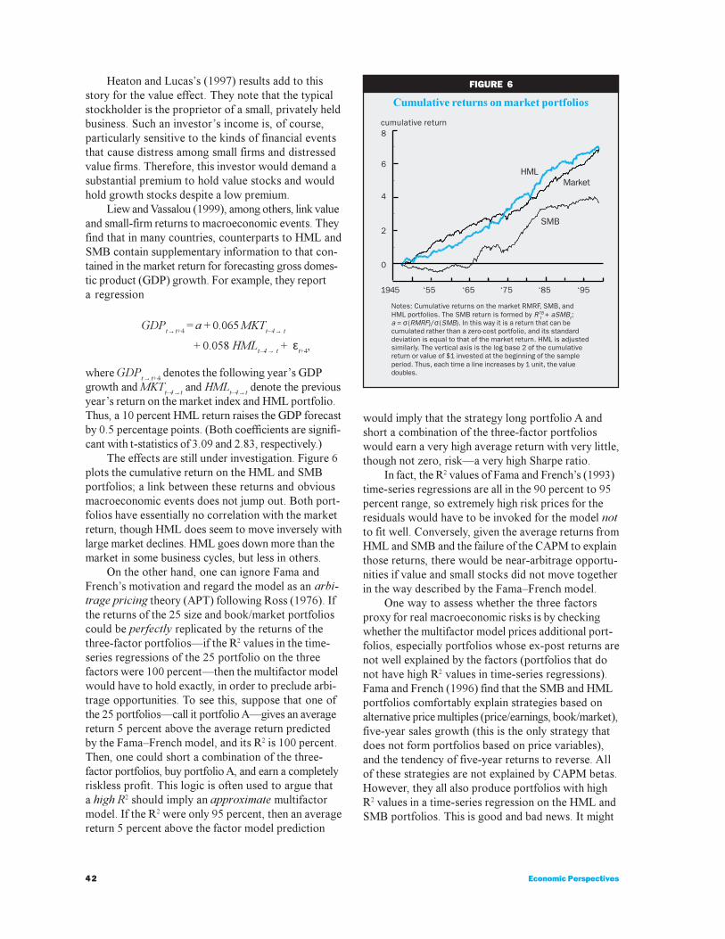
The effects are still under investigation. Figure 6plots the cumulative return on the HML and SMBportfolios; a link between these returns and obviousmacroeconomic events does not jump out. Both port-folios have essentially no correlation with the marketreturn, though HML does seem to move inversely withlarge market declines. HML goes down more than themarket in some business cycles, but less in others.

On the other hand, one can ignore Fama andFrench�s motivation and regard the model as an arbi-trage pricing theory (APT) following Ross (1976). Ifthe returns of the 25 size and book/market portfolioscould be perfectly replicated by the returns of thethree-factor portfolios�if the R2 values in the time-series regressions of the 25 portfolio on the threefactors were 100 percent�then the multifactor modelwould have to hold exactly, in order to preclude arbi-trage opportunities. To see this, suppose that one ofthe 25 portfolios�call it portfolio A�gives an averagereturn 5 percent above the average return predictedby the Fama�French model, and its R2 is 100 percent.Then, one could short a combination of the three-factor portfolios, buy portfolio A, and earn a completelyriskless profit. This logic is often used to argue thata high R2 should imply an approximate multifactormodel. If the R2 were only 95 percent, then an averagereturn 5 percent above the factor model prediction

would imply that the strategy long portfolio A andshort a combination of the three-factor portfolioswould earn a very high average return with very little,though not zero, risk�a very high Sharpe ratio.

In fact, the R2 values of Fama and French�s (1993)time-series regressions are all in the 90 percent to 95percent range, so extremely high risk prices for theresiduals would have to be invoked for the model notto fit well. Conversely, given the average returns fromHML and SMB and the failure of the CAPM to explainthose returns, there would be near-arbitrage opportu-nities if value and small stocks did not move togetherin the way described by the Fama�French model.

One way to assess whether the three factorsproxy for real macroeconomic risks is by checkingwhether the multifactor model prices additional port-folios, especially portfolios whose ex-post returns arenot well explained by the factors (portfolios that donot have high R2 values in time-series regressions).Fama and French (1996) find that the SMB and HMLportfolios comfortably explain strategies based onalternative price multiples (price/earnings, book/market),five-year sales growth (this is the only strategy thatdoes not form portfolios based on price variables),and the tendency of five-year returns to reverse. Allof these strategies are not explained by CAPM betas.However, they all also produce portfolios with highR2 values in a time-series regression on the HML andSMB portfolios. This is good and bad news. It might

FIGURE 6

Cumulative returns on market portfolios

cumulative return

Notes: Cumulative returns on the market RMRF, SMB, andHML portfolios. The SMB return is formed by RTB

t + aSMBt;a = σ(RMRF)/σ(SMB). In this way it is a return that can becumulated rather than a zero-cost portfolio, and its standarddeviation is equal to that of the market return. HML is adjustedsimilarly. The vertical axis is the log base 2 of the cumulativereturn or value of $1 invested at the beginning of the sampleperiod. Thus, each time a line increases by 1 unit, the valuedoubles.

8

1945

6

4

2

0

‘55 ‘65 ‘75 ‘85 ‘95

HMLMarket

SMB


mean that the model is a good APT, and that the sizeand book/market characteristics describe the majorsources of priced variation in all stocks. On the otherhand, it might mean that these extra ways of construct-ing portfolios just haven�t identified other sources ofpriced variation in stock returns. (Fama and French,1996, also find that HML and SMB do not explainmomentum, despite high R2 values. I discuss thisanomaly below.) The portfolios of stocks sorted byindustry in Fama and French (1997) have lower R2

values, and the model works less well.A final concern is that the size and book/market

premiums seem to have diminished substantially inrecent years. The sharp decline in the SMB portfolioreturn around 1980 when the small-firm effect was firstpopularized is obvious in figure 6. In Fama and French�s(1993) initial samples, 1960�90, the HML cumulativereturn starts about one-half (0.62) below the marketand ends up about one-half (0.77) above the market.On the log scale of the figure, this corresponds to Famaand French�s report that the HML average return isabout double (precisely, 20.62+0.77 = 2.6 times) that ofthe market. However, over the entire sample of theplot, the HML portfolio starts and ends at the sameplace and so earns almost exactly the same as themarket. From 1990 to now, the HML portfolio losesabout one-half relative to the market, meaning an inves-tor in the market has increased his money one and ahalf times as much as an HML investor. (The actualnumber is 0.77 so the market return is 20.77 = 1.71 timesbetter than the HML return.)

Among other worries, if the average returns declineright after publication it suggests that the anomaliesmay simply have been overlooked by a large fractionof investors. As they move in, prices go up further,helping the apparent anomaly for a while. But once alarge number of investors have moved in to includesmall and value stocks in their portfolios, the anoma-lous high average returns disappear.

However, average returns are hard to measure.There have been previous ten- to 20-year periods inwhich small stocks did very badly, for example the1950s, and similar decade-long variations in the HMLpremium. Also, since SMB and HML have a beta ofessentially zero on the market, any upward trend is aviolation of the CAPM and says that investors canimprove their overall mean�variance tradeoff by takingon some of the HML or SMB portfolio.

Macroeconomic factorsI focus on the size and value factors because they

provide the most empirically successful multifactormodel and have attracted much industry as well as

academic attention. Several authors have used macro-economic variables as factors. This procedure examinesdirectly whether stock performance during bad macro-economic times determines average returns. Jagan-nathan and Wang (1996) and Reyfman (1997) uselabor income; Chen, Roll, and Ross (1986) look atindustrial production and inflation among other vari-ables; and Cochrane (1996) looks at investment growth.All these authors find that average returns line upwith betas calculated using the macroeconomic indica-tors. The factors are theoretically easier to motivate,but none explains the value and size portfolios aswell as the (theoretically less solid, so far) size andvalue factors.

Merton�s (1973, 1971) theory says that variableswhich predict market returns should show up as fac-tors that explain cross-sectional variation in averagereturns. Campbell (1996) is the lone test I know of todirectly address this question. Cochrane (1996) andJagannathan and Wang (1996) perform related tests inthat they include �scaled return� factors, for example,market return at t multiplied by d/p ratio at t � 1; theyfind that these factors are also important in under-standing cross-sectional variation in average returns.

The next step is to link these more fundamentallydetermined factors with the empirically more success-ful value and small-firm factor portfolios. Because ofmeasurement difficulties and selection biases, funda-mentally determined macroeconomic factors will neverapproach the empirical performance of portfolio-basedfactors. However, they may help to explain which port-folio-based factors really work and why.

Predictable returns

The view that risky asset returns are largely unpre-dictable, or that prices follow �random walks,� remainsimmensely successful ( Malkiel, 1990, is a classic andreadable introduction). It is also widely ignored.

Unpredictable returns mean that if stocks wentup yesterday, there is no exploitable tendency for themto decline today because of �profit taking� or to contin-ue to rise today because of �momentum.� �Technical�signals, including analysis of past price movementstrading volume, open interest, and so on are close touseless for forecasting short-term gains and losses.As I write, value funds are reportedly suffering largeoutflows because their stocks have done poorly inthe last few months, leading fund investors to movemoney into blue-chip funds that have performed bet-ter (New York Times Company, 1999). Unpredictablereturns mean that this strategy will not do anythingfor investors� portfolios over the long run except rackup trading costs. If funds are selling stocks, then


contrarian investors must be buying them, but un-predictable returns mean that this strategy can notimprove performance either. If one can not system-atically make money, one can not systematicallylose money either.

As discussed in the introduction, researchersonce believed that stock returns (more precisely, theexcess returns on stocks over short-term interestrates) were completely unpredictable. It now turnsout that average returns on the market and individualsecurities do vary over time and that stock returnsare predictable. Alas for would-be technical traders,much of that predictability comes at long horizonsand seems to be associated with business cycles andfinancial distress.

Market returnsTable 1 presents a regression that forecasts re-

turns. Low prices�relative to dividends, book value,earnings, sales, or other divisors�predict higher sub-sequent returns. As the R2 values in table 1 show,these are long-horizon effects: Annual returns areonly slightly predictable and month-to-month returnsare still strikingly unpredictable, but returns at five-yearhorizons seem very predictable. (Fama and French, 1989,is an excellent reference for this kind of regression).

The results at different horizons are reflectionsof a single underlying phenomenon. If daily returnsare very slightly predictable by a slow-moving vari-able, that predictability adds up over long horizons.For example, you can predict that the temperature inChicago will rise about one-third of a degree per dayin spring. This forecast explains very little of the dayto day variation in temperature, but tracks almost allof the rise in temperature from January to July. Thus,the R2 rises with horizon.

Precisely, suppose that we forecast returns witha forecasting variable x, according to

1

2

1 1 1

1 1

)

) .

R R a bx

x c x

t tTB

t t

t t t

+ + +

+ +

- = + +

= + +

e

r d

Small values of b and R2 in equation 1 and a largecoefficient ρ in equation 2 imply mathematically thatthe long-horizon regression as in table 1 has a largeregression coefficient b and large R2.

This regression has a powerful implication: Stocksare in many ways like bonds. Any bond investor un-derstands that a string of good past returns that push-es the price up is bad news for subsequent returns.Many stock investors see a string of good past returnsand become elated that we seem to be in a �bull

market,� concluding future stock returns will be goodas well. The regression reveals the opposite: A stringof good past returns which drives up stock pricesis bad news for subsequent stock returns, as it isfor bonds.

Long-horizon return predictability was first doc-umented in the volatility tests of Shiller (1981) andLeRoy and Porter (1981). They found that stock pric-es vary far too much to be accounted for by chang-ing expectations of subsequent cash flows; thuschanging discount rates or expected returns mustaccount for variation in stock prices. These volatilitytests turn out to be almost identical to regressionssuch as those in table 1 (Cochrane, 1991).

Momentum and reversalSince a string of good returns gives a high price,

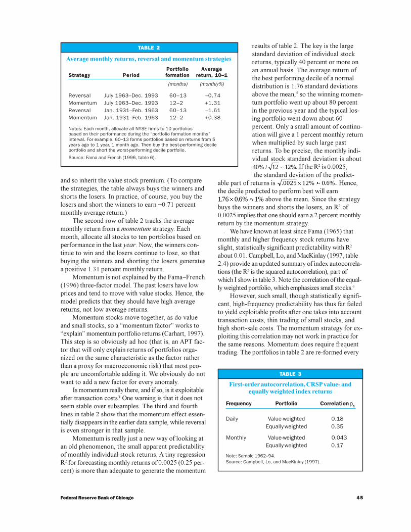
it is not surprising that individual stocks that dowell for a long time (and reach a high price) subse-quently do poorly, and stocks that do poorly for along time (and reach a low price, market value, or mar-ket to book ratio) subsequently do well. Table 2, takenfrom Fama and French (1996) confirms this hunch.(Also, see DeBont and Thaler, 1985, and Jegadeeshand Titman, 1993.)

The first row in table 2 tracks the average monthlyreturn from the reversal strategy. Each month, allocateall stocks to ten portfolios based on performancefrom year �5 to year �1. Then, buy the best-perform-ing portfolio and short the worst-performing portfolio.This strategy earns a hefty �0.74 percent monthlyreturn.4 Past long-term losers come back and pastwinners do badly. Fama and French (1996) verify thatthese portfolio returns are explained by their three-factor model. Past winners move with value stocks,

TABLE 1

OLS regression of excess returns onprice/dividend ratio

Horizon k b Standard error R2

1 year –1.04 0.33 0.172 years –2.04 0.66 0.263 years –2.84 0.88 0.385 years –6.22 1.24 0.59

Notes: OLS regressions of excess returns (value-weightedNYSE–Treasury bill rate) on value-weighted price/dividendratio.

R R a b P Dt t kVW

t t kTB

t t t k� + � + +- = + +( / ) .e

Rt→t+k indicates the k year return. Standard errors use GMMto correct for heteroskedasticity and serial correlation.


and so inherit the value stock premium. (To comparethe strategies, the table always buys the winners andshorts the losers. In practice, of course, you buy thelosers and short the winners to earn +0.71 percentmonthly average return.)

The second row of table 2 tracks the averagemonthly return from a momentum strategy. Eachmonth, allocate all stocks to ten portfolios based onperformance in the last year. Now, the winners con-tinue to win and the losers continue to lose, so thatbuying the winners and shorting the losers generatesa positive 1.31 percent monthly return.

Momentum is not explained by the Fama�French(1996) three-factor model. The past losers have lowprices and tend to move with value stocks. Hence, themodel predicts that they should have high averagereturns, not low average returns.

Momentum stocks move together, as do valueand small stocks, so a �momentum factor� works to�explain� momentum portfolio returns (Carhart, 1997).This step is so obviously ad hoc (that is, an APT fac-tor that will only explain returns of portfolios orga-nized on the same characteristic as the factor ratherthan a proxy for macroeconomic risk) that most peo-ple are uncomfortable adding it. We obviously do notwant to add a new factor for every anomaly.

Is momentum really there, and if so, is it exploitableafter transaction costs? One warning is that it does notseem stable over subsamples. The third and fourthlines in table 2 show that the momentum effect essen-tially disappears in the earlier data sample, while reversalis even stronger in that sample.

Momentum is really just a new way of looking atan old phenomenon, the small apparent predictabilityof monthly individual stock returns. A tiny regressionR2 for forecasting monthly returns of 0.0025 (0.25 per-cent) is more than adequate to generate the momentum

results of table 2. The key is the largestandard deviation of individual stockreturns, typically 40 percent or more onan annual basis. The average return ofthe best performing decile of a normaldistribution is 1.76 standard deviationsabove the mean,5 so the winning momen-tum portfolio went up about 80 percentin the previous year and the typical los-ing portfolio went down about 60percent. Only a small amount of continu-ation will give a 1 percent monthly returnwhen multiplied by such large pastreturns. To be precise, the monthly indi-vidual stock standard deviation is about40% 12 12%./ £ If the R2 is 0.0025, the standard deviation of the predict-

able part of returns is . .0025 12% 0 6%.� £ Hence,the decile predicted to perform best will earn176 0 6% 1%. .� £ above the mean. Since the strategybuys the winners and shorts the losers, an R2 of0.0025 implies that one should earn a 2 percent monthlyreturn by the momentum strategy.

We have known at least since Fama (1965) thatmonthly and higher frequency stock returns haveslight, statistically significant predictability with R2

about 0.01. Campbell, Lo, and MacKinlay (1997, table2.4) provide an updated summary of index autocorrela-tions (the R2 is the squared autocorrelation), part ofwhich I show in table 3. Note the correlation of the equal-ly weighted portfolio, which emphasizes small stocks.6

However, such small, though statistically signifi-cant, high-frequency predictability has thus far failedto yield exploitable profits after one takes into accounttransaction costs, thin trading of small stocks, andhigh short-sale costs. The momentum strategy for ex-ploiting this correlation may not work in practice forthe same reasons. Momentum does require frequenttrading. The portfolios in table 2 are re-formed every

TABLE 2

Average monthly returns, reversal and momentum strategies

Portfolio AverageStrategy Period formation return, 10–1

(months) (monthly %)

Reversal July 1963–Dec. 1993 60–13 –0.74Momentum July 1963–Dec. 1993 12–2 +1.31Reversal Jan. 1931–Feb. 1963 60–13 –1.61Momentum Jan. 1931–Feb. 1963 12–2 +0.38

Notes: Each month, allocate all NYSE firms to 10 portfoliosbased on their performance during the “portfolio formation months”interval. For example, 60–13 forms portfolios based on returns from 5years ago to 1 year, 1 month ago. Then buy the best-performing decileportfolio and short the worst-performing decile portfolio.

Source: Fama and French (1996, table 6).

TABLE 3

First-order autocorrelation, CRSP value- andequally weighted index returns

Frequency Portfolio Correlation ρ 1

Daily Value-weighted 0.18Equally weighted 0.35

Monthly Value-weighted 0.043Equally weighted 0.17

Note: Sample 1962–94.Source: Campbell, Lo, and MacKinlay (1997).


month. Annual winners and losers will not changethat often, but the winning and losing portfolio mustbe turned over at least once per year. In a quantitativeexamination of this effect, Carhart (1997) concludesthat momentum is not exploitable after transactioncosts are taken into account. Moskowitz and Grinblatt(1999) note that most of the apparent gains from themomentum strategy come from short positions insmall illiquid stocks. They also find that a large partof momentum profits come from short positions takenin November. Many investors sell losing stocks towardthe end of December to establish tax losses. By short-ing illiquid losing stocks in November, an investorcan profit from the selling pressure in December. Thisis also an anomaly, but it seems like a glitch rather thana central principle of risk and return in asset markets.

Even if momentum and reversal are real and asstrong as indicated by table 2, they do not justify muchof the trading based on past results that many inves-tors seem to do. To get the 1 percent per month

momentum return, one buys a portfolio that has typi-cally gone up 80 percent in the last year, and shorts aportfolio that has typically gone down 60 percent.Trading between stocks and fund categories such asvalue and blue-chip with smaller past returns yieldsat best proportionally smaller results. Since much ofthe momentum return seems to come from shortingsmall illiquid stocks, mild momentum strategies mayyield even less. And we have not quantified the sub-stantial risk of momentum strategies.

Bonds

The venerable expectations model of the termstructure specifies that long-term bond yields areequal to the average of expected future short-term bondyields (see box 2). For example, if long-term bond yieldsare higher than short-term bond yields�if the yieldcurve is upward sloping�this means that short-termrates are expected to rise in the future. The rise in fu-ture short-term rates means that investors can expect

BOX 2

Bond definitions and expectations hypothesis

Let ptN( ) denote the log of the N year discount

bond price at time t. The N period continuously

compounded yield is defined by yN

ptN

tN( ) ( ) .= -

1

The continuously compounded holding periodreturn is the selling price less the buying price,hpr p pt

Nt

Nt

N+ +

-

= -1 11( ) ( ) ( ) . The forward rate is the rate

at which an investor can contract today to borrowmoney N � 1 years from now, and repay that moneyN years from now. Since an investor can synthe-size a forward contract from discount bonds, theforward rate is determined from discount bondprices by

f p ptN

tN

tN( ) ( – ) ( )– .=

1

The �spot rate� refers, by contrast with a for-ward rate, to the yield on any bond for which theinvestor take immediate delivery. Forward ratesare typically higher than spot rates when the yieldcurve rises, since the yield is the average of inter-vening forward rates,

yN

f f f ftN

t t t tN( ) ( ) ( ) ( ( )( ... ).= + + + +

1 1 2 3)

The expectations hypothesis states that theexpected log or continuously compounded returnshould be the same for any bond strategy. Thisstatement has three mathematically equivalentexpressions:

1. The forward rate should equal the expectedvalue of the future spot rate,

f E ytN

t t N( ) ( )( ).=

+ -11

2. The expected holding period return should bethe same on bonds of any maturity

E hpr E hpr yt tN

t tM

t( ) ( ) .( ) ( ) ( )+ +

= =1 11

3. The long-term bond yield should equal theaverage of the expected future short rates,

yN

E y y ytN

t t t t N( ) ( ) ( ) ( )( ... ).= + + +

+ + -

1 11

11

1

The expectations hypothesis is often amend-ed to allow a constant risk premium of undeter-mined sign in these equations. Its violation is thenoften described as evidence for a �time-varyingrisk premium.�

The expectations hypothesis is not quite thesame thing as risk-neutrality, because the expectedlog return is not equal to the log expected return.However, the issues here are larger than the differ-ence between the expectations hypothesis andstrict risk-neutrality.


the same rate of return whether they hold a long-termbond to maturity or roll over short-term bonds withinitially low returns and subsequent higher returns.

As with the CAPM and the view that stock returnsare independent over time, a new round of researchhas significantly modified this traditional view ofbond markets.

Table 4 calculates the average return on bondsof different maturities. The expectations hypothesisseems to do pretty well. Average holding period returnsdo not seem very different across bond maturities,despite the increasing standard deviation of longer-maturity bond returns. The small increase in averagereturns for long-term bonds, equivalent to a slightaverage upward slope in the yield curve, is usuallyexcused as a �liquidity premium.� Table 4 is just thetip of an iceberg of successes for the expectationsmodel. Especially in times of significant inflation andexchange rate instability, the expectations hypothesishas done a very good first-order job of explaining theterm structure of interest rates.

However, if there are times when long-term bondsare expected to do better and other times when short-term bonds are expected to do better, the unconditionalaverages in table 4 could still show no pattern. Simi-larly, one might want to check whether a forward ratethat is unusually high forecasts an unusual increasein spot rates.

Table 5 updates Fama and Bliss�s (1987) classicregression tests of this idea. Panel A presents a regres-sion of the change in yields on the forward-spotspread. (The forward-spot spread measures the slopeof the yield curve.) The expectations hypothesis pre-dicts a slope coefficient of 1.0, since the forward rateshould equal the expected future spot rate. If, forexample, forward rates are lower than expected futurespot rates, traders can lock in a borrowing positionwith a forward contract and then lend at the higherspot rate when the time comes.

Instead, at a one-year horizon we find slope co-efficients near zero and a negative adjusted R2. For-ward rates one year out seem to have no predictivepower whatsoever for changes in the spot rate oneyear from now. On the other hand, by four years out,we see slope coefficients within one standard error of1.0. Thus, the expectations hypothesis seems to dopoorly at short (one-year) horizons, but much betterat longer horizons.

If the expectations hypothesis does not work atone-year horizons, then there is money to be made�one must be able to foresee years in which short-termbonds will return more than long-term bonds and viceversa, at least to some extent. To confirm this implica-tion, panel B of table 5 runs regressions of the one-yearexcess return on long-term bonds on the forward-spot spread. Here, the expectations hypothesis pre-dicts a coefficient of zero: No signal (including the

TABLE 4

Zero-coupon bond returns

Maturity Average holding Standard StandardN period return error deviation

1 5.83 0.42 2.832 6.15 0.54 3.653 6.40 0.69 4.664 6.40 0.85 5.715 6.36 0.98 6.58

Note: Continuously compounded one-year holding periodreturns on zero-coupon bonds of varying maturity. Annualdata from CRSP 1953–97.

TABLE 5

Forecasts based on forward-spot spread

A. Change in yields B. Holding period returns

Standard Standard Standard Standarderror, error, Adjusted error, error, Adjusted

N Intercept intercept Slope slope R2 Intercept intercept Slope slope R2

1 0.10 0.3 –0.10 0.36 –0.020 –0.1 0.3 1.10 0.36 0.16

2 –0.01 0.4 0.37 0.33 0.005 –0.5 0.5 1.46 0.44 0.19

3 –0.04 0.5 0.41 0.33 0.013 –0.4 0.8 1.30 0.54 0.10

4 –0.30 0.5 0.77 0.31 0.110 –0.5 1.0 1.31 0.63 0.07

Notes: OLS regressions, 1953–97 annual data. Panel A estimates the regression y (1) t+n – yt

(1) = a +b (ft(N+1) – yt

(1)) + ε t+N

and panel B estimates the regression hpr (N)t+1

–yt(1) = a + b (f t

(N+1) – y (1)t ) + ε t+1

, where yt(N) denotes the N-year bond yield at

date t; ft(N) denotes the N-period ahead forward rate; and hpr (N

t+)1 denotes the one-year holding period return at date t + 1

on an N-year bond. Yields and returns in annual percentages.


forward-spot spread) should be able to tell you thatthis is a particularly good time for long bonds versusshort bonds, as the random walk view of stock pricessays that no signal should be able to tell you thatthis is a particularly good or bad day for stocks versusbonds. However, the coefficients in panel B are allabout 1.0. A high forward rate does not indicate thatinterest rates will be higher one year from now; itseems to indicate that investors will earn that muchmore by holding long-term bonds.7

Of course, there is risk. The R2 values are all 0.1�0.2, about the same values as the R2 from the d/p re-gression at a one-year horizon, so this strategy willoften go wrong. Still, 0.1�0.2 is not zero, so the strat-egy does pay off more often than not, in violation ofthe expectations hypothesis. Furthermore, the for-ward-spot spread is a slow-moving variable, typicallyreversing sign once per business cycle. Thus, the R2

builds with horizon as with the d/p regression, peak-ing in the 30 percent range (Fama and French, 1989).

Foreign exchange

Suppose interest rates are higher in Germanythan in the U.S. Does this mean that one can earnmore money by investing in German bonds? Thereare several reasons that the answer might be no.First, of course, is default risk. Governments havedefaulted on bonds in the past and may do so again.Second, and more important, is the risk of devalua-tion. If German interest rates are 10 percent and U.S.interest rates are 5 percent, but the euro falls 5 per-cent relative to the dollar during the year, you makeno more money holding the German bondsdespite their attractive interest rate. Sincelots of investors are making this calcula-tion, it is natural to conclude that an inter-est rate differential across countries onbonds of similar credit risk should revealan expectation of currency devaluation.The logic is exactly the same as that of theexpectations hypothesis in the term struc-ture. Initially attractive yield or interest ratedifferentials should be met by an offsettingevent so that you make no more moneyon average in one maturity or currencyversus another.8

As with the expectations hypothesisin the term structure, the expected depreci-ation view still constitutes an importantfirst-order understanding of interest ratedifferentials and exchange rates. For exam-ple, interest rates in east Asian currencieswere very high on the eve of the recentcurrency tumbles, and many banks were

making tidy sums borrowing at 5 percent in dollars tolend at 20 percent in local currencies. This suggeststhat traders were anticipating a 15 percent devalua-tion, or a smaller chance of a larger devaluation, whichis exactly what happened. Many observers attributehigh nominal interest rates in troubled economies to�tight monetary policy� aimed at defending the cur-rency. In reality, high nominal rates reflect a large prob-ability of inflation and devaluation�loose monetarypolicy�and correspond to much lower real rates.

Still, does a 5 percent interest rate differentialcorrespond to a 5 percent expected depreciation, ordoes some of it represent a high expected return fromholding debt in that country�s currency? Further-more, while expected depreciation is clearly a largepart of the interest rate story in high-inflation econo-mies, how does the story play out in economies likethe U.S. and Germany, where inflation rates divergelittle but exchange rates still fluctuate a large amount?

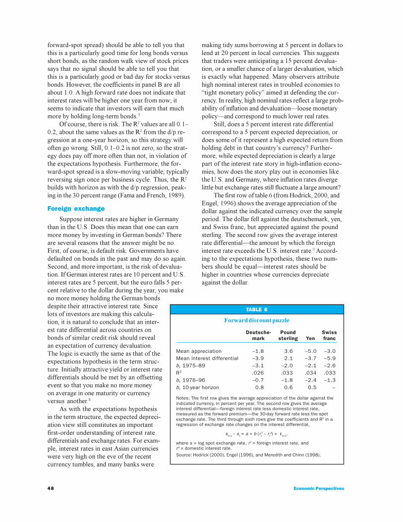
The first row of table 6 (from Hodrick, 2000, andEngel, 1996) shows the average appreciation of thedollar against the indicated currency over the sampleperiod. The dollar fell against the deutschemark, yen,and Swiss franc, but appreciated against the poundsterling. The second row gives the average interestrate differential�the amount by which the foreigninterest rate exceeds the U.S. interest rate.9 Accord-ing to the expectations hypothesis, these two num-bers should be equal�interest rates should behigher in countries whose currencies depreciateagainst the dollar.

TABLE 6

Forward discount puzzle

Deutsche- Pound Swissmark sterling Yen franc

Mean appreciation –1.8 3.6 –5.0 –3.0Mean interest differential –3.9 2.1 –3.7 –5.9b, 1975–89 –3.1 –2.0 –2.1 –2.6R2 .026 .033 .034 .033b, 1976–96 –0.7 –1.8 –2.4 –1.3b, 10-year horizon 0.8 0.6 0.5 –

Notes: The first row gives the average appreciation of the dollar against theindicated currency, in percent per year. The second row gives the averageinterest differential—foreign interest rate less domestic interest rate,measured as the forward premium—the 30-day forward rate less the spotexchange rate. The third through sixth rows give the coefficients and R2 in aregression of exchange rate changes on the interest differential,

st+1 – st = a + b (rt

f – rtd) + εt+1

,

where s = log spot exchange rate, r f = foreign interest rate, andrd = domestic interest rate.Source: Hodrick (2000), Engel (1996), and Meredith and Chinn (1998).


The second row shows roughly the expected pat-tern. Countries with steady long-term inflation havesteadily higher interest rates and steady depreciation.The numbers in the first and second rows are notexactly the same, but exchange rates are notoriouslyvolatile so these averages are not well measured. Ho-drick (2000) shows that the difference between thefirst and second rows is not statistically differentfrom zero. This fact is analogous to the evidence intable 4 that the expectations hypothesis works wellon average for U.S. bonds.

As in the case of bonds, however, we can askwhether times of temporarily higher or lower interestrate differentials correspond to times of above- andbelow-average depreciation as they should. The thirdand fifth rows of table 6 update Fama�s (1984) regres-sion tests. The number here should be +1.0 in eachcase�1 percentage point extra interest differentialshould correspond to 1 percentage point extra ex-pected depreciation. On the contrary, as table 6 shows,a higher than usual interest rate abroad seems to leadto further appreciation. This is the forward discountpuzzle. See Engel (1996) and Lewis (1995) for recentsurveys of the avalanche of academic work investigat-ing whether this puzzle is really there and why.

The R2 values shown in table 6 are quite low.However, like d/p and the term spread, the interest dif-ferential is a slow-moving forecasting variable, so thereturn forecast R2 builds with horizon. Bekaert andHodrick (1992) report that the R2 rises to the 30 percentto 40 percent range at six-month horizons and thendeclines. That�s high, but not 100 percent; takingadvantage of any predictability strategy is quite risky.

The puzzle does not say that one earns more byholding bonds from countries with higher interestrates than others. Average inflation, depreciation,and interest rate differentials line up as they should.The puzzle does say that one earns more by holdingbonds from countries whose interest rates are higherthan usual relative to U.S. interest rates (and viceversa). The fact that the �usual� rate of depreciationand interest differential changes through time will, ofcourse, diminish the out-of-sample performance ofthese trading rules.

One might expect that exchange rate depreciationworks better for long-run exchange rates, as the expec-tations hypothesis works better for long-run interestrate changes. The last row of table 6, taken fromMeredith and Chinn (1998) verifies that this is so.Ten-year exchange rate changes are correctly forecastby the interest differentials of ten-year bonds.

Mutual funds

Studying the returns of funds that follow a spe-cific strategy gives us a way to assess whether thatstrategy works in practice, after transaction costsand other trading realities are taken into account.Studying the returns of actively managed funds tellsus whether the time, talent, and effort put into pickingsecurities pays off. Most of the literature on evaluatingfund performance is devoted to the latter question.

A large body of empirical work, starting withJensen (1969), finds that actively managed funds, onaverage, underperform the market index. I use datafrom Carhart (1997), whose measures of fund perfor-mance account for survivor bias. Survivor bias arisesbecause funds that do badly go out of business.Therefore, the average fund that is alive at any pointin time has an artificially good track record.

As with the stock portfolios in figure 1, the funddata in figure 7 show a definite correlation betweenbeta and average return: Funds that did well took onmore market risks. A cross-sectional regression line isa bit flatter than the line drawn through the Treasurybill and market return, but this is a typical result ofmeasurement error in the betas. (The data are annual,and many funds are only around for a few years, con-tributing to beta measurement error.) The average fundunderperforms the line connecting Treasury bills andthe market index by 1.23 percent per year (that is, theaverage alpha is �1.23 percent).

The wide dispersion in fund average returns infigure 7 is a bit surprising. Average returns vary acrossfunds almost as much as they do across individualstocks. This fact implies that the majority of fundsare not holding well-diversified portfolios that wouldreduce return variation, but rather are loading up onspecific bets.

Initially, the fact that the average fund underper-forms the market seems beside the point. Perhaps theaverage fund is bad, but we want to know whetherthe good funds are any good. The trouble is, we mustsomehow distinguish skill from luck. The only wayto separate skill from luck is to group funds basedon some ex-ante observable characteristic, and thenexamine the average performance of the group. Ofcourse, skillful funds should have done better, onaverage, in the past, and should continue to do betterin the future. Thus, if there is skill in stock picking,we should see some persistence in fund performance.However, a generation of empirical work found no per-sistence at all. Funds that did well in the past were nomore likely to do well in the future.


Since the average fund underperforms the market,and fund returns are not predictable, we concludethat active management does not generate superiorperformance, especially after transaction costs andfees. This fact is surprising. Professionals in almostany field do better than amateurs. One would expectthat a trained experienced professional who spendsall day reading about markets and stocks should beable to outperform simple indexing strategies. Even ifentry into the industry is so easy that the averagefund does not outperform simple indexes one wouldexpect a few stars to outperform year after year, asgood teams win championship after championship.Alas, the contrary fact is the result of practically everyinvestigation, and even the anomalous results docu-ment very small effects.

Funds and valueGiven the value, small-firm, and predictability

effects, the idea that funds cluster around the marketline is quite surprising. All of these new facts implyinescapably that there are simple, mechanical strate-gies that can give a risk/reward ratio greater than thatof buying and holding the market index. Fama and

French (1993) report that the HML port-folio alone gives nearly double the marketSharpe ratio�the same average return athalf the standard deviation. Why don�tfunds cluster around a risk/reward linesignificantly above the market�s?

Of course, we should not expect allfunds to cluster around a higher risk/re-ward tradeoff. The average investorholds the market, and if funds are largeenough, so must the average fund. Indexfunds, of course, will perform like the in-dex. Still, the typical actively managedfund advertises high mean and, perhaps,low variance. No fund advertises cuttingaverage returns in half to spare investorsexposure to nonmarket sources of risk.Such funds, apparently aimed at mean�variance investors, should clusteraround the highest risk/reward tradeoffavailable from mechanical strategies(and more, if active management doesany good). Most troubling, funds whosay they follow value strategies don�toutperform the market either. For example,Lakonishok, Shleifer, and Vishny (1992,table 3) find that the average value fundunderperforms the S&P500 by 1 percentjust like all the others.

We can resolve this contradiction ifwe think that fund managers were simply unaware ofthe possibilities offered by our new facts, and so(despite the advertising) were not really followingthem. That seems to be the implication of figure 7,which sorts funds by their HML beta. One would ex-pect the high-HML beta funds to outperform the mar-ket line. But the cutoff for the top one-third of fundsis only a HML beta of 0.3, and even that may be high(many funds don�t last long, so betas are poorly mea-sured; the distribution of measured betas is widerthan the actual distribution). Thus, the �value funds�were really not following the �value strategy� thatearns the HML returns; if they were doing so theywould have HML betas of 1.0. Similarly, Lakonishok,Shleifer, and Vishny�s (1992) documentation of valuefunds� underperformance reveals that their marketbeta is close to 1.0. These results imply that valuefunds are not really following a value strategy, sincetheir returns correlate with the market portfolio and notthe value portfolio.

Interestingly, the number of value and small-capfunds (as revealed by their betas, not their marketingclaims) is increasing quickly. Before 1990, 14 percentof funds had measured SMB betas greater than 1.0,

FIGURE 7

Average returns of mutual funds vs. market betas

average return

Notes: Average returns of mutual funds over the Treasury bill rate versus theirmarket betas. Sample consists of all funds with average total net assetsgreater than $25 million and more than 25 percent of their assets in stocks,in the Carhart (1996) database. Data sample 1962–96. The average excessreturn is computed as E(Ri– Rf ) = ai + βi x 9%. ai and βi are computed from atime-series regression of fund annual excess returns on market annual excessreturns over the life of the fund. The o, +, and x labels in the figure sort fundsinto thirds based on their regression coefficient h on the Fama–French value(HML) portfolio. The breakpoints are h = –0.084, 0.34. The dashed line givesthe fit of a cross-sectional ordinary least squares regression of ai on βi ; Thesolid line connects the Treasury bill (β and excess return = 0) and the marketreturn (β = 1, excess return = 9%).

0.25

0.20

0.15

0.10

0.05

0.00

–0.05

–0.10

–0.50 0.00 0.50 1.00 1.50beta

= value= neutral= growth


and 12 percent had HML betas greater than 1.0. Inthe full sample, both numbers have doubled to 22percent and 23 percent. This trend suggests thatfunds will, in the future, be much less well describedby the market index.

The view that funds were unaware of value strat-egies, and are now moving quickly to exploit them,can explain why most funds still earn near the marketreturn, rather than the higher value return. However,this view contradicts the view that the value premiumis an equilibrium risk premium, that is, that everyoneknew about the value returns but chose not to investall along because they feared the risks of value strat-egies. If it is not an equilibrium risk premium, it won�tlast long.

Persistence in fund returnsThe fund counterpart to momentum in stock re-

turns has been more extensively investigated thanthe value and size effects. Fund returns have alsobeen found to be persistent. Since such persistencecan be interpreted as evidence for persistent skill inpicking stocks, it is not surprising that it has attract-ed a great deal of attention, starting with Hendricks,Patel, and Zeckhauser (1993).

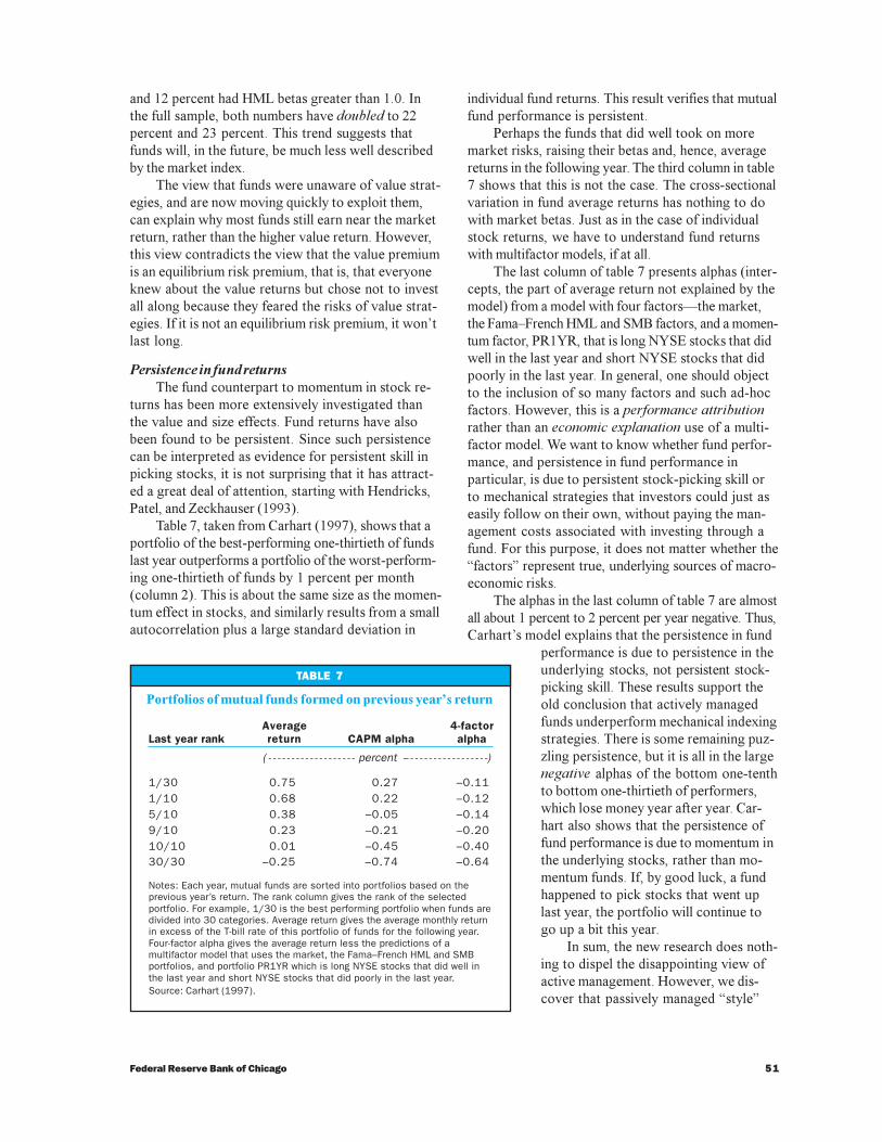
Table 7, taken from Carhart (1997), shows that aportfolio of the best-performing one-thirtieth of fundslast year outperforms a portfolio of the worst-perform-ing one-thirtieth of funds by 1 percent per month(column 2). This is about the same size as the momen-tum effect in stocks, and similarly results from a smallautocorrelation plus a large standard deviation in

individual fund returns. This result verifies that mutualfund performance is persistent.

Perhaps the funds that did well took on moremarket risks, raising their betas and, hence, averagereturns in the following year. The third column in table7 shows that this is not the case. The cross-sectionalvariation in fund average returns has nothing to dowith market betas. Just as in the case of individualstock returns, we have to understand fund returnswith multifactor models, if at all.

The last column of table 7 presents alphas (inter-cepts, the part of average return not explained by themodel) from a model with four factors�the market,the Fama�French HML and SMB factors, and a momen-tum factor, PR1YR, that is long NYSE stocks that didwell in the last year and short NYSE stocks that didpoorly in the last year. In general, one should objectto the inclusion of so many factors and such ad-hocfactors. However, this is a performance attributionrather than an economic explanation use of a multi-factor model. We want to know whether fund perfor-mance, and persistence in fund performance inparticular, is due to persistent stock-picking skill orto mechanical strategies that investors could just aseasily follow on their own, without paying the man-agement costs associated with investing through afund. For this purpose, it does not matter whether the�factors� represent true, underlying sources of macro-economic risks.

The alphas in the last column of table 7 are almostall about 1 percent to 2 percent per year negative. Thus,Carhart�s model explains that the persistence in fund

performance is due to persistence in theunderlying stocks, not persistent stock-picking skill. These results support theold conclusion that actively managedfunds underperform mechanical indexingstrategies. There is some remaining puz-zling persistence, but it is all in the largenegative alphas of the bottom one-tenthto bottom one-thirtieth of performers,which lose money year after year. Car-hart also shows that the persistence offund performance is due to momentum inthe underlying stocks, rather than mo-mentum funds. If, by good luck, a fundhappened to pick stocks that went uplast year, the portfolio will continue togo up a bit this year.

In sum, the new research does noth-ing to dispel the disappointing view ofactive management. However, we dis-cover that passively managed �style�

TABLE 7

Portfolios of mutual funds formed on previous year�s return

Average 4-factorLast year rank return CAPM alpha alpha

( - - - - - - - - - - - - - - - - - - - percent -- - - - - - - - - - - - - - - - - -)

1/30 0.75 0.27 –0.111/10 0.68 0.22 –0.125/10 0.38 –0.05 –0.149/10 0.23 –0.21 –0.2010/10 0.01 –0.45 –0.4030/30 –0.25 –0.74 –0.64

Notes: Each year, mutual funds are sorted into portfolios based on theprevious year’s return. The rank column gives the rank of the selectedportfolio. For example, 1/30 is the best performing portfolio when funds aredivided into 30 categories. Average return gives the average monthly returnin excess of the T-bill rate of this portfolio of funds for the following year.Four-factor alpha gives the average return less the predictions of amultifactor model that uses the market, the Fama–French HML and SMBportfolios, and portfolio PR1YR which is long NYSE stocks that did well inthe last year and short NYSE stocks that did poorly in the last year.Source: Carhart (1997).


portfolios can earn returns that are not explained bythe CAPM.

Catastrophe insuranceA number of prominent funds have earned very

good returns (and others, spectacular losses) by fol-lowing strategies such as convergence trades andimplicit put options. These strategies may also reflecthigh average returns as compensation for nonmarketdimensions of risk. They have not been examined atthe same level of detail as the value and small-capstrategies, so I offer a possible interpretation ratherthan a documented one.

Convergence trades take strong positions in verysimilar securities that have small price differences.For example, a 29.5-year Treasury bond typicallytrades at a slightly higher yield (lower price) than a30-year Treasury bond. (This was the most famousbet placed by LTCM. See Lewis, 1999.) A convergencetrade puts a strong short position on the expensivesecurity and a strong long position on the cheap secu-rity. This strategy is often mislabeled an �arbitrage.�However, the securities are similar, not identical. Thespread between 29.5- and 30-year Treasury bondsreflects the lower liquidity of the shorter maturityand the associated difficulty of selling it in a financialpanic. It is possible for this spread to widen. Nonethe-less, panics are rare, and the average returns inall the years when they do not happen may more thanmake up for the spectacular losses when they do.

Put options protect investors from large pricedeclines. The volatility smile in put option pricesreflects the surprisingly high prices of such options,compared with the small probability of large marketcollapses (even when one calibrates the probabilitydirectly, rather than using the log-normal distributionof the Black�Scholes formula). Writers of out-of-the-money puts collect a fee every month; in a rare marketcollapse they will pay out a huge sum, but if the proba-bility of the collapse is small enough, the averagereturns may be quite good.

All of these strategies can be thought of as catas-trophe insurance (Hsieh and Fung, 1999). Most ofthe time they earn a small premium. Once in a greatwhile they lose a lot, and they lose a lot in times offinancial catastrophe, when most investors are reallyanxious that the value of their investments not evap-orate. Therefore, it is economically plausible thatthese strategies can earn positive average returns,even when we account for stock market risk via theCAPM and we correctly measure the small probabilitiesof large losses.

The difficulty in empirically estimating the trueaverage return of such strategies, of course, is that

rare events are rare. Many long samples will give afalse sense of security because �the big one� thatjustifies the premium happened not to hit.

The value, yield curve, and foreign exchangestrategies I survey above also exhibit features ofcatastrophe insurance. Value stocks may earn highreturns because distressed stocks will all go bankruptin a financial panic. Buying bonds of countries withhigh interest rates leaves one open to the small chanceof a large devaluation, and such devaluation isespecially likely to happen in a global financial panic.Similarly, buying long-term bonds in the depth of arecession when the yield curve is upward slopingmay expose one to a small risk of a large inflation.

If these interpretations bear out, they also sug-gest that the premiums�the average returns fromholding stocks sensitive to HML or from followingthe bond and foreign exchange strategies�may beoverstated in the data. The markets have had an unusu-ally good 50 years, and devastating financialpanics have not happened.

Implications of the new facts

While the list of new facts appears long, similarpatterns show up in every case. Prices reveal slow-moving market expectations of subsequent returns,because potential offsetting events seem sluggishor absent. The patterns suggest that investors canearn substantial average returns by taking on therisks of recession and financial stress. In addition,there is a small positive autocorrelation of high-frequency returns.

The effects are not completely new. We haveknown since the 1960s that high-frequency returnsare slightly predictable, with R2 of 0.01 to 0.1 in dailyto monthly returns. These effects were dismissedbecause there didn�t seem to be much one could doabout them. A 51/49 bet is not very attractive, especial-ly if there is any transaction cost. Also, the increasedSharpe ratio (mean excess return/standard deviation)from exploiting predictability is directly related to theforecast R2, so a tiny R2, even if exploitable, did notseem important. Now, we have a greater understand-ing of the potential importance of these effects andtheir economic interpretations.

For price effects, we now realize that the R2 riseswith horizon when the forecasting variables are slow-moving. Hence, a small R2 at short horizons can mean areally substantial R2 in the 30 percent to 50 percentrange at longer horizons. Also, the nature of theseeffects suggests the kinds of additional sources ofpriced risk that theorists had anticipated for 20 years.For momentum effects, the ability to sort stocks and


funds into momentum-based portfolios means that verysmall predictability times portfolios with huge past re-turns gives important subsequent returns, though it isnot totally clear that this amplification of the small pre-dictability really does survive transaction costs.

Price-based forecastsIf expected returns rise, prices are driven down,

since future dividends or other cash flows are discount-ed at a higher rate. A �low� price, then, can reveal a mar-ket expectation of a high expected or required return.10

Most of our results come from this effect. Lowprice/dividend, price/earnings, or price/book valuessignal times when the market as a whole will have highaverage returns. Low market value (price times shares)relative to book value signals securities or portfoliosthat earn high average returns. The �small-firm� ef-fect derives from low prices�other measures of sizesuch as number of employees or book value alonehave no predictive power for returns (Berk, 1997).The �five-year reversal� effect derives from the factthat five years of poor returns lead to a low price. Ahigh long-term bond yield means that the price of long-term bonds is �low,� and this seems to signal a timeof good long-term bond returns. A high foreign inter-est rate means a low price on foreign bonds, and thisseems to indicate good returns on the foreign bonds.

The most natural interpretation of all these effectsis that the expected or required return�the risk pre-mium�on individual securities as well as the marketas a whole varies slowly over time. Thus we can trackmarket expectations of returns by watching price/div-idend, price/earnings, or book/market ratios.

Absent offsetting eventsIn each case, an apparent difference in yield

should give rise to an offsetting movement, but doesnot seem to do so. Something should be predictableso that returns are not predictable, and it is not. Figure8 provides a picture of the results in table 5. Supposethat the yield curve is upward sloping as in panel A.What does this mean? If the expectations model weretrue, the forward rates plotted against maturity wouldtranslate one for one to the forecast of future spotrates in panel B, as plotted in the black line marked�Expectations model.� A high long-term bond yieldrelative to short-term bond yields should not mean ahigher expected long-term bond return. Subsequentshort rates should rise, cutting off the one-periodadvantage of long-term bonds and raising the multi-year advantage of short-term bonds.

In figure 8, panel b, the colored line marked �Esti-mates� shows the actual forecast of future spot inter-est rates from the results in table 5. The essence of thephenomenon is sluggish adjustment of the shortrates. The short rates do eventually rise to meet theforward rate forecasts, but not as quickly as the for-ward rates predict they should. Short-term yieldsshould be forecastable so that returns are not fore-castable. In fact, yields are almost unforecastable,so, mechanically, bond returns are. The roughly 1.0coefficients in panel B of table 5 mean that a 1 per-centage point increase in the forward rate translatesinto a 1 percentage point increase in expected return.It seems that old fallacy of confusing bond yieldswith their expected returns for the first year containsa grain of truth.

FIGURE 8

percent

Yield curve and forecast one-year interest rates

A. Current yield curve

forecast interest rate

B. Forecast one-year interest rates

1 2

7.0

6.5

6.0

5.5

4.5

5.0

3 4 5maturity, years

1 2 3 4 5time in the future, years

7.0

6.5

6.0

5.5

4.5

5.0

Notes: Assuming that the current yield curve is as shown in panel A, the black line in panelB gives the forecast from the expectations hypothesis, in which case forward rates today arethe forecast of future spot rates. The colored line in panel B gives the actual forecast of futurespot rates, constructed from the estimates in table 5.

Forward rate

Yield

Estimates

Expectationsmodel


In the same way, a high dividend yield on a stockor portfolio should mean that dividends grow moreslowly over time, or, for individual stocks, that the firmhas taken on more market risk and will have a highermarket beta. These tendencies seem to be completelyabsent. Dividend/price ratios do not seem to forecastdividend growth and, hence, (mechanically) theyforecast returns. The one-year coefficient in table 1 isvery close to 1.00, meaning that a 1 percentage pointincrease in the dividend yield translates into a 1 per-centage point increase in return. It seems that the oldfallacy of confusing increased dividend yield with in-creased total return does contain a grain of truth.

A high foreign interest rate relative to domesticinterest rates should not mean a higher expected re-turn. We should see, on average, an offsetting depre-ciation. But here, the coefficients are even larger than1.0. An interest rate differential seems to predict a fur-ther appreciation. It seems that the old fallacy ofconfusing interest rate differentials across countrieswith expected returns, forgetting about depreciation,also contains a grain of truth.

Economic interpretationThe price-based predictability patterns suggest

a premium for holding risks related to recession andeconomy-wide financial distress. Stock and bond pre-dictability are linked: The term spread (forward-spot,or long yield�short yield) forecasts stock returns aswell as bond returns (Fama and French, 1989). Fur-thermore, the term spread is one of the best variablesfor forecasting business cycles. It rises steeply at thebottom of recessions and is inverted at the top of aboom. Return forecasts are high at the bottom of abusiness cycle and low at the top of a boom. Valueand small-cap stocks are typically distressed. Empiri-cally successful economic models of the recession anddistress premiums are still in their infancy (Campbelland Cochrane, 1999, is a start), but the story is atleast plausible and the effects have been expectedby theorists for a generation.

To make this point come to life, think concretelyabout what you have to do to take advantage of thepredictability strategies. You have to buy stocks orlong-term bonds at the bottom, when stock prices arelow after a long and depressing bear market, in thebottom of a recession or the peak of a financial panic.This is a time when few people have the guts or thewallet to buy risky stocks or risky long-term bonds.Looking across stocks rather than over time, you haveto invest in value or small-cap companies, with yearsof poor past returns, poor sales, or on the edge ofbankruptcy. You have to buy stocks that everyoneelse thinks are dogs. Then, you have to sell stocks

and long-term bonds in good times, when stock pricesare high relative to dividends, earnings, and othermultiples and the yield curve is flat or inverted sothat long-term bond prices are high. You have to sellthe popular growth stocks, with good past returns,good sales, and earnings growth.

You have to sell now, and the stocks that youshould sell are the blue-chips that everyone else seemsto be buying. In fact, the market timing strategies saidto sell long ago; if you did so, you would have missedmuch of the runup in the Dow past the 6,000 point. Val-ue stocks too have missed most of the recent marketrunup. However, this shouldn�t worry you�a strategythat holds risks uncorrelated with the market must un-derperform the market close to half of the time.

If this feels uncomfortable, what you�re feelingis risk. If you�re uncomfortable watching the marketpass you by, perhaps you don�t really only care aboutlong-run mean and variance; you also care aboutdoing well when the market is doing well. If you wantto stay fully invested in stocks, perhaps you too feelthe time-varying aversion to or exposure to risk thatdrives the average investor to stay fully investeddespite low prospective returns.

This line of explanation for the foreign exchangepuzzle is still a bit farther off (see Engel, 1996, for asurvey; Atkeson, Alvarez, and Kehoe, 1999, offer arecent stab at an explanation). The strategy leads in-vestors to invest in countries with high interest rates.High interest rates are often a sign of monetary insta-bility or other economic trouble, and thus may meanthat the investments are more exposed to the risks ofglobal financial stress or a global recession than areinvestments in the bonds of countries with low interestrates, which are typically enjoying better times.

Return correlationMomentum and persistent fund performance

explained by a momentum factor are different from theprice-based predictability results. In both cases, theunderlying phenomenon is a small predictability ofhigh-frequency returns. The price-based predictabili-ty strategies make this predictability important byshowing that, with a slow-moving forecasting variable,the R2 builds over horizon. Momentum, however, isbased on a fast-moving forecast variable�the previ-ous year�s return. Therefore, the R2 declines ratherthan building with horizon. Momentum makes thesmall predictability of high-frequency returns signifi-cant in a different way, by forming portfolios of extremewinners and losers. The large volatility of returns meansthat the extreme portfolios will have extreme pastreturns, so only a small continuation of past returnsgives a large current return.


It would be appealing to understand momentumas a reflection of slowly time-varying average expectedreturns or risk premiums, like the price-based predict-ability strategies. If a stock�s average return rises fora while, that should make returns higher both todayand tomorrow. Thus, a portfolio of past winners willcontain more than its share of stocks that performedwell because their average returns were higher, alongwith stocks that performed well due to luck. Theaverage return of such a portfolio should be highertomorrow as well.

Unfortunately, this story has to posit a substan-tially different view of the underlying process forvarying expected returns than is needed to explaineverything else. The trouble is that a surprise increasein expected returns means that prices will fall, sincedividends are now discounted at a greater rate. Thisis the phenomenon we have relied on to explain whylow price/dividend, price/earnings, book/market,value, and size forecast higher subsequent returns.Therefore, positive correlation of expected returnstypically yields a negative correlation of realizedreturns. To get a positive correlation of realized returnsout of slow expected return variation, you have toimagine that an increase in average returns today iseither highly correlated with a decrease in expectedfuture dividend growth or with a decrease in expectedreturns in the distant future (an impulse responsethat starts positive but is negative at long horizons).Campbell, Lo, and MacKinlay (1997) provide a quan-titative exposition of these effects.

Furthermore, momentum returns have not yetbeen linked to business cycles or financial distress ineven the informal way that I suggested for price-basedstrategies. Thus, momentum still lacks a plausibleeconomic interpretation. To me, this adds weight tothe view that it isn�t there, it isn�t exploitable, or itrepresents a small illiquidity (tax-loss selling of smallilliquid stocks) that will be quickly remedied once afew traders understand it.

Remaining doubtsThe size of all these effects is still somewhat

in question. It is always hard to measure averagereturns of risky strategies. The standard formulas / T for the standard error of the mean, togetherwith the high volatility σ of any strategy, means thatone needs 25 years of data to even start to measureaverage returns. With σ = 16 percent (typical of theindex), even T = 25 years means that one standarderror is 16/5 ≅ 3 percent per year, and a two-standarderror confidence interval runs plus or minus 6 percent-age points. This is not much smaller than the averagereturns we are trying to measure. In addition, all of

these facts are highly influenced by the small proba-bility of rare events, which makes measuring averagereturns even harder.

Finally, viewed the right way, we have very fewdata points with which to evaluate predictability. Theterm premium and interest rate differentials only changesign with the business cycle, and the dividend/priceratio only crosses its mean once every generation.The history of interest rates and inflation in the U.S.is dominated by the increase, through two recessions,to a peak in 1980 and then a slow decline after that.

Many of the anomalous risk premiums seem tobe declining over time. Figure 6 shows the decline inthe HML and SMB premiums, and the same may betrue of the predictability effects. The last three yearsof high market returns have cut the estimated returnpredictability from the dividend/price ratio in half.This fact suggests that at least some of the premiumthe new strategies yielded in the past was due to thefact that they were simply overlooked.

Was it really clear to average investors in 1947 or1963 (the beginning of the data samples) that stockswould earn 9 percent over bonds, and that the strate-gy of buying distressed small stocks would doubleeven that return for the same level of risk? Would av-erage investors have changed their portfolios with thisknowledge? Or would they have stayed pat, explain-ing that these returns are earned as a reward for riskthat they were not willing to take? Was it clear thatbuying stocks at the bottom in the mid-1970s wouldyield so much more than even that high average re-turn? If we interpret the premiums measured in sam-ple as true risk premiums, the answer must be yes.If the answer is no, then at least some part of thepremium was luck and will disappear in the future.

Since the premiums are hard to measure, one istempted to put less emphasis on them. However, theyare crucial to our interpretation of the facts. TheCAPM is perfectly consistent with the fact that thereare additional sources of common variation. For ex-ample, it was long understood that stocks in the sameindustry move together; the fact that value or smallstocks also move together need not cause a ripple.The surprise is that investors seem to earn an averagereturn premium for holding these additional sourcesof common movement, whereas the CAPM predictsthat (given beta) they should have no effect on aportfolio�s average returns.

The behavior of funds also suggests the �over-looked strategy� interpretation. As explained earlier,fund returns still cluster around the market line. It turnsout that very few fund returns actually followed thevalue or other return-enhancing strategies. However,the number of small, value, and related funds�funds


that actually do follow the strategies�has increaseddramatically in recent years. It might be possible toexplain this in a way consistent with the idea that in-vestors knew the premiums were there all along, butsuch an argument is obviously strained.

Conclusion

In sum, it now seems that investors can earn asubstantial premium for holding dimensions of riskunrelated to market movements, such as recession-related or distress-related risk. Investors earn thesepremiums by following strategies, such as value and

NOTES

REFERENCES

1The market also tends to go down in recessions; howeverrecessions can be unusually severe or mild for a given level ofmarket return. What counts here is the severity of the recessionfor a given market return. Technically, we are consideringbetas in a multiple regression that includes both the marketreturn and a measure of recessions. See box 1.

2I thank Gene Fama for providing me with these data.

3The rest of the paragraph is my interpretation, not Fama andFrench�s. They focus on the firm�s financial distress, while Ifocus on the systematic distress, since idiosyncratic distresscannot deliver a risk price.

4Fama and French do not provide direct measures of standard de-viations for these portfolios. One can infer, however, from thebetas, R2 values, and standard deviation of the market and factorportfolios that the standard deviations are roughly one to twotimes that of the market return, so Sharpe ratios of these strate-gies are comparable to that of the market return in sample.

5We are looking for

E r r xrf r dr

f r drx

x

( | )( )

( ),� =

I

I

�

�

where x is defined as the top one-tenth cutoff,

x f r dr�

I =( ) .1

10

With a normal distribution, x = 1.2816σ and E(r|r≥x) = 1.755σ.

6The index autocorrelations suffer from some upward biassince some stocks do not trade every day. Individual stockautocorrelations are generally smaller, but are enough toaccount for the momentum effect.

7Panel B is really not independent evidence, since the coeffi-cients in panels A and B of table 5 are mechanically linked. Forexample, 1.14 + (�0.14) = 1.0, and this holds as an accountingidentity. Fama and Bliss (1987) call them �complementaryregressions.�

8As with bonds, the expectations hypothesis is slightly differentfrom pure risk neutrality since the expectation of the log isnot the log of the expectation. Again, the size of the phenom-ena we study swamps this distinction.

9The data are actually the spread between the forward exchangerate and the spot exchange rate, but this quantity must equalthe interest rate differential in order to preclude arbitrage.

10This effect is initially counterintuitive. One might supposethat a higher average return would attract investors, raisingprices. But the higher prices, for a given dividend stream, mustreduce subsequent average returns. High average returns persist,in equilibrium, when investors fear the increased risks of anasset and try to sell, lowering prices.

growth, market-timing possibilities generated by returnpredictability, dynamic bond and foreign exchangestrategies, and maybe even a bit of momentum. Theexact size of the premiums and the economic natureof the underlying risks is still a bit open to question,but researchers are unlikely to go back to the simpleview that returns are independent over time and thatthe CAPM describes the cross section.

The next question is, What should investors dowith this information? The article, �Portfolio advicefor a multifactor world,� also in this issue, addressesthat question.

Atkeson, Andrew, Fernando Alvarez, and PatrickKehoe, 1999, �Volatile exchange rates and the forwardpremium anomaly: A segmented asset market view,�University of Chicago, working paper.

Banz, R. W., 1981, �The relationship between returnand market value of common stocks,� Journal ofFinancial Economics, Vol. 9, No. 1, pp. 3�18.

Bekaert, Geert, and Robert J. Hodrick, 1992, �Char-acterizing predictable components in excess returns

on equity and foreign exchange markets,� Journal ofFinance, Vol. 47, No. 2, June, pp. 467�509.

Berk, Jonathan, 1997, �Does size really matter?,�Financial Analysts Journal, Vol. 53, September/October, pp. 12�18.

Campbell, John Y., 1996, �Understanding risk and re-turn,� Journal of Political Economy, Vol. 104, No. 2,April, pp. 298�345.


Campbell, John Y., and John H. Cochrane, 1999, �Byforce of habit: A consumption-based explanation ofaggregate stock market behavior,� Journal of PoliticalEconomy, Vol. 107, No. 2, April, pp. 205�251.

Campbell, John Y., Andrew W. Lo, and A. CraigMacKinlay, 1997, The Econometrics of FinancialMarkets, Princeton, NJ: Princeton University Press.

Carhart, Mark M., 1997, �On persistence in mutualfund performance,� Journal of Finance, Vol. 52, No.1, March, pp. 57�82.

Chen, Nai-Fu, Richard Roll, and Stephen A. Ross,1986, �Economic forces and the stock market,� Journalof Business, Vol. 59, No. 3, July, pp. 383�403.

Cochrane, John H., 1997, �Where is the market going?Uncertain facts and novel theories,� EconomicPerspectives, Federal Reserve Bank of Chicago, Vol.21, No. 6, November/December, pp. 3�37.

, 1996, �A cross-sectional test of an invest-ment-based asset pricing model,� Journal of PoliticalEconomy, Vol. 104, No. 3, June, pp. 572�621.

, 1991, �Volatility tests and efficient mar-kets: Review essay,� Journal of Monetary Econom-ics; Vol. 27, No. 3, June, pp. 463-485.

Daniel, Kent, David Hirshleifer, and AvanidharSubrahmanyam, 1998, �Investor psychology andsecurity market under- and overreactions,� Journalof Finance, Vol. 3, No. 6, December, pp. 1839�1885.

DeBondt, Werner F. M., and Richard H. Thaler,1985, �Does the stock market overreact?,� Journalof Finance, Vol. 40, No. 3, pp. 793�805.

Engel, Charles, 1996, �The forward discount anomalyand the risk premium: A survey of recent evidence,�Journal of Empirical Finance, Vol. 3, pp. 123�192.

Fama, Eugene F. 1991, �Efficient markets II,� Journalof Finance, Vol. 46, No. 5, December, pp. 1575�1617.

, 1984, �Forward and spot exchangerates,� Journal of Monetary Economics, Vol. 14,No. 3, November, pp. 319�338.

, 1970, �Efficient capital markets: A reviewof theory and empirical work,� Journal of Finance,Vol. 25, No. 2, May, pp. 383�417.

, 1965, �The behavior of stock market prices,�Journal of Business, Vol. 38, No. 1, pp. 34�105.

Fama, Eugene F., and Robert R. Bliss, 1987, �Theinformation in long-maturity forward rates,� AmericanEconomic Review, Vol. 77, No. 4, September,pp. 680�692.

Fama, Eugene F., and Kenneth R. French, 1997, �Indus-try costs of equity,� Journal of Financial Economics,Vol. 43, No. 2, February, pp. 153�193.

, 1996, �Multifactor explanations of asset-pricing anomalies,� Journal of Finance, Vol. 51, No. 1,March, pp, 55�84.

, 1995, �Size and book-to-market factors inearnings and returns,� Journal of Finance, Vol. 50,No.1, March, pp. 131�155.

, 1993, �Common risk factors in the returnson stocks and bonds,� Journal of Financial Econom-ics, Vol. 33, No. 1, February, pp. 3�56.

, 1989, �Business conditions and expectedreturns on stocks and bonds,� Journal of FinancialEconomics, Vol. 25, No. 1, November, pp. 23�49.

Heaton, John, and Deborah Lucas, 1997, �Portfoliochoice and asset prices: The importance of entrepre-neurial risk,� Northwestern University, manuscript.

Hendricks, Darryll, Jayendu Patel, and RichardZeckhauser, 1993, �Hot hands in mutual funds:Short-term persistence of performance,� Journal ofFinance, Vol. 48, No. 1, March, pp. 93�130.

Hodrick, Robert, 2000, International FinancialManagement, Englewood Cliffs, NJ: Prentice-Hall,forthcoming.

Hsieh, David, and William Fung, 1999, �Hedge fundrisk management,� Duke University, working paper.

Jagannathan, Ravi, and Zhenyu Wang, 1996, �Theconditional CAPM and the cross-section of expectedreturns,� Journal of Finance, Vol. 51, No. 1, March,pp. 3�53.

Jegadeesh, Narasimham, and Sheridan Titman,1993, �Returns to buying winners and selling losers:Implications for stock market efficiency,� Journal ofFinance, Vol. 48, No. 1, March, pp. 65�91.

Jensen, Michael C., 1969, �The pricing of capitalassets and evaluation of investment portfolios,�Journal of Business, Vol. 42, No. 2, April, pp. 167�247.


Lakonishok, Josef, Andrei Shleifer, and Robert W.Vishny, 1992, �The structure and performance of themoney management industry,� Brookings Papers onEconomic Activity: Microeconomics 1992, Washing-ton, DC, pp. 339�391

LeRoy, Stephen F., and Richard D. Porter, 1981, �Thepresent-value relation: Tests based on implied vari-ance bounds,� Econometrica, Vol. 49, No. 3, May, pp.555�574.

Lewis, Karen, K., 1995, �Puzzles in internationalfinancial markets,� in Handbook of InternationalEconomics, Vol. 3, G. Grossman and K. Rogoff (eds.),Amsterdam, New York, and Oxford: Elsevier ScienceB.V, pp. 1913�1971.

Lewis, Michael, 1999, �How the eggheads cracked,�New York Times Magazine, January 24,pp. 24�42.

Liew, Jimmy, and Maria Vassalou, 1999, �Can book-to-market, size and momentum be risk factors that pre-dict economic growth?,� Columbia University,working paper.

MacKinlay, A. Craig, 1995, �Multifactor models donot explain deviations from the CAPM,� Journal ofFinancial Economics, Vol. 38, No. 1, pp. 3�28.

Malkiel, Burton, 1990, A Random Walk Down WallStreet, New York: Norton.

Markowitz, H., 1952, �Portfolio selection,� Journalof Finance, Vol. 7, No. 1, March, pp. 77�99.

Meredith, Guy, and Menzie D. Chinn, 1998, �Long-horizon uncovered interest rate parity,� National Bu-reau of Economic Research, working paper, No. 6797.

Merton, Robert C., 1973, �An intertemporal capitalasset pricing model,� Econometrica, Vol. 41, No. 5,September, pp. 867�887.

, 1971, �Optimum consumption and port-folio rules in a continuous time model,� Journal ofEconomic Theory, Vol. 3, No. 4, pp. 373�413.

, 1969, �Lifetime portfolio selection underuncertainty: The continuous time case,� Review ofEconomics and Statistics, Vol. 51, No. 3, August,pp. 247�257.

Moskowitz, Tobias, and Mark Grinblatt, 1999, �Taxloss selling and return autocorrelation: New evidence,�University of Chicago, working paper.

, 1998, �Do industries explain momen-tum?,� University of Chicago, CRSP working paper,No. 480.

New York Times Company, 1999, �Mutual fundsreport: What�s killing the value managers?,� NewYork Times, April 4, Section 3, p. 29.

Reyfman, Alexander, 1997, �Labor market risk andexpected asset returns,� University of Chicago,Ph.D. thesis.

Ross, S. A., 1976, �The arbitrage theory of capitalasset pricing,� Journal of Economic Theory, Vol. 13,No. 3, December, pp. 341�360.

Samuelson, Paul A., 1969, �Lifetime portfolio selec-tion by dynamic stochastic programming,�� Reviewof Economics and Statistics, Vol. 51, No. 3, August,pp. 239�246.

Sargent, Thomas J., 1993, Bounded Rationality inMacroeconomics, Oxford: Oxford University Press.

Shiller, Robert J., 1981, �Do prices move too muchto be justified by subsequent changes in divi-dends?,� American Economic Review, Vol. 71, No. 3,June, pp. 421�436.

new facts in finance - booth school of business36 economic perspectives new facts in finance john h....

Documents