new efficient, simple and user friendly artificial fuzzy ... · applications. the fuzzy logic...

Journal of Multidisciplinary Engineering Science and Technology (JMEST)

ISSN: 2458-9403

Vol. 6 Issue 2, February - 2019

www.jmest.org

JMESTN42352831 9509

New Efficient, Simple And User Friendly Artificial Fuzzy Logic Control Algorithm Design

Method Farhan A. Salem

1,2

1Industrial engineering program, Department of Mechanical Engineering, Faculty of Engineering, Taif University, Taif 888, , Saudi Arabia.

2Alpha center for Engineering Studies and Technology Researches, Amman, Jordan.

Email: [email protected]

Abstract—This paper proposes new generalized, direct and user friendly artificial fuzzy control algorithm, applicable to control a variety of systems, to result in acceptable stability and medium fastness of response. The proposed fuzzy control algorithm requires setting up the ranges for universes of discourse of inputs and output by just inserting the value of control unit operating voltage. When needed, to further adjust resulted response in terms of speeding up and/or reducing overshoot, oscillation and/or error, two options are proposed. The first is using three introduced soft tuning parameters with soft tuning ranges and effects. Second is accomplished by adding pseudo-derivative feedback control. For validation, the proposed fuzzy control algorithm is simulated and tested to control a wide range of different systems, simulation results showed applicability of proposed design to result in acceptable stability and medium fastness of response

Keywords—Artificial intelligence, Fuzzy algorithm, algorithm Design.

I. INTRODUCTION

The terms control system design can be referred, but not limited to, one of the following forms; a) for intelligent control algorithms, developing a knowledge base, Inference mechanisms; and communication interfaces or b) the process of selecting feedback gains (poles and zeros) that meet design specifications in a closed-loop control system, or, c) writing corresponding control algorithm/program (e.g. for PLC, CNC or Microcontroller) to control the process.

A variety of possible physical-controller and algorithm subsystems options are available. The physical-controller subsystem, can be structured, basically, around six basic forms of programmable control system: Personal computer (PC), Microcomputer, Microcontroller, Digital signal processors (DSP), Application specific integrated circuits (ASICs) and Programmable logic controller (PLC), also, there are a variety of control algorithms exits, including: ON-OFF, PID modes, Feedforward, adaptive, intelligent control algorithms [1].

Intelligent control methodologies have been developed to address in a systematic way, problems of control which cannot be formulated and studied in the conventional differential/difference equation mathematical framework [2]. Intelligent control algorithms include; Fuzzy logic, neural network, Expert Systems, Genetic, Bayesian and Neuro- Fuzzy algorithms.

The scope of this paper is limited to artificial fuzzy logic control algorithm design. The purpose of this work is to develop a generalized, direct, simple and user-friendly fuzzy logic control algorithm design, which can be applied to control a wide range of systems to result in acceptable stability, and medium fastness of response. In literature, different such works can be found, based on trial and error [3], artificial neural network(ANN) [4], genetic algorithms (GA) [5] based algorithms, and clustering methods [6]. It has been proven that all these methods work very well. However, it should be noted that they are not just fuzzy systems. They are hybrid systems, which combine other intelligent methods such as neural networks and genetic algorithms with the fuzzy logic. Although the hybrid systems are more powerful and adaptive, they require high level algorithms with time consuming processes that are not desirable in control applications. The fuzzy logic controllers appeared in literature are mostly modeled for specific applications rather than for general cases [7].

II. The proposed fuzzy logic control algorithm design

II.I Fuzzy logic control algorithm

Fuzzy logic was first proposed in [8]. fuzzy logic control algorithm is a practical alternative methodology to represent, manipulate and implement a smart human’s heuristic knowledge (thinking, understanding, sensing, decision-making and experience) about how to control a system [9], using this knowledge, it provides a convenient method for constructing nonlinear controllers, it integrates human’s heuristic knowledge of skilled operators and/or control engineer, then express it using a natural description language (descriptive model), as rules on how to control the process and achieve high-performance control, these rules are incorporated into a fuzzy controller that emulates the decision-making process of the human. Disadvantages of fuzzy control

http://www.jmest.org/


ISSN: 2458-9403


www.jmest.org

JMESTN42352831 9510

include that fuzzy controllers with fixed structures fail to stabilize the plant under wide variations of the operating condition.

II.II Types of Fuzzy control algorithms

Different forms of fuzzy concepts application in control system/algorithm design have been studied in the literature, as shown in Figure 1, fuzzy controllers can be classified into the following forms; (1) Well-known direct action fuzzy logic control (FLC), which uses the error and the change rate of the error for determining the control action [10]. (2) The fuzzy PID control that can be classified into the following major categories according to the way of their construction; (a) Fuzzy Gain Scheduling, (Figure 2(b)) when the gains of the conventional PID controller are tuned on-line in terms of the knowledge base and fuzzy inference, while still the conventional PID controller generates the control signal [11, 12], (b) The hybrid fuzzy-PID controller (HFPID) (Figure 2(c)) examples include ; using both fuzzy and PID control algorithms, according to distance to target position, one of both controllers is selected to generate control signal. HFPIDCR uses fuzzy logic controller and PID with coupled rules (HFPIDCR) which combines both PI and PD actions [10]. Neuro-fuzzy which uses a combination of fuzzy logic and neural networks. (c) Direct action Fuzzy PID control are further classified according to the number of the input variables; namely single input, two input, and three input fuzzy PID controllers[11] two input direct action Fuzzy PID can be expanded to fuzzy-PD, fuzzy-PI, fuzzy-adaptive algorithms.

Figure 1 A classification of fuzzy controllers [11]

Figure 2(a) Fuzzy control structure

Figure 2(b) application of Fuzzy algorithm to assign the correct va;5lues of PID/PD/PI parameters

Figure 2(c) Block diagram of hybrid fuzzy PID controller type.

III. The proposed fuzzy control algorithm design

The time response of the control error (e) for a step input can be represented by the generalized step response error of a second order system shown in Figure 3. Refereeing to this figure and depending on region ( I : X), each one of error (e), change rate of the error (de) and one output variable (plant/drive input signal (Δu)) has three different options for the signs to be assigned; positive (P), negative (N), and zero (Z). The signs of Δu in those regions are listed in Table 1, where the signs of e and Δe are used to determine the signs of Δu, which in turn determines whether the overall control signal is to be changed. The sign of Δu should be positive if u is required to be increased and it should be negative otherwise 7]. Based on this the decision rule base can be developed.

Figure 3 Operating regions of the time responses of error and error change for a generalized second order system [7].

Fuzzy Control algorithms

Fuzzy PID Fuzzy Non-PID

Direct action TypeFuzzy gain

scheduling type Hybrid type

Single input

Twoinputs

Threeinputs

Rule Knowledge base

Inference mechanism

Fuzz

ific

ati

on

De

Fuzz

ific

ati

on

Output

Input(1)

Input(2)

PID modesR(s)

Rule Knowledge base

Inference mechanism

Fuzz

ific

atio

n

DeF

uzz

ific

atio

n

Output

Input(1)

Input(2)

Plant

Sensor

E(s) C(s)

Fuzzy PID modes-gains scheduling

Fuzzy PID controller

Conventional PID controller

ErrorControl

signal

IF e < ??



ISSN: 2458-9403


www.jmest.org

JMESTN42352831 9511

Table 1 : The signs of basic control action .

Operating regions

I II II IV V VI VII VIII IX X

E + 0 - - 0 + + - + 0

ΔE - - - + + + - 0 0 0

ΔU + - - - + + + - + 0

III.I First fuzzy control algorithm design

As shown in Figure 4(a,b,c,d), the proposed algorithm is fallen under direct action Fuzzy PID control, (PI/PD type) with two inputs and one output variable, namely error (e), change rate of the error (de) and plant/drive input signal (u). The linguistic variables used are defined with the seven linguistic values. These values are; NB-negative big, NM-negative medium, NS-negative small, ZE-zero, PS-positive small, PM-positive medium, PB-positive big. Triangular membership function is used to represent linguistic values. The linguistic variables are normalized in interval of [−1, 1] (see Figure 4(c,d,e)). Membership function ranges for the two input and one output are all distributed alike and with ranges; [0, 0, 0],[0, 0.35, 7][0.35, 07, 1][0.7, 1, 1.35]. Rule base was determined by using experience and engineering mentality [14] and testing for different systems, these rules can be modified to improve proposed algorithm. Rules are written in a rule base look-up Table 2. Nonlinear characteristic of rule base can be seen in Figure 5. As a rule inference method, Mamdani method is selected, centroid method was used for defuzzification [15,16].

As shown in Figure 4(a), three scaling factors (gains) (a, b, c), with corresponding three tuning parameters (α, β, γ) with initial value of unity, (α = β =γ =1), are used to adjust the ranges of the universes of discourse for each of the two inputs and one output of fuzzy controller. The scaling factors are given by Eq.(1).

an inverse relationship exists between the input scaling gains and the ranges of the universes of discourse, such that; (a) if input tuning gain = 1, then there is no effect on the membership functions, (b) if input tuning gains < 1, then the membership functions are uniformly “spread out” by a factor of 1/(factor value), this means the linguistics quantify larger numbers, (c) if input tuning > 1, the membership functions are uniformly “contracted” this means the linguistics quantify smaller numbers. An opposite effect is seen for the output scaling gain.

Tuning these factors has the effect of speeding up response and/or reducing overshoot, oscillation and/or error.

1

1

in

in

in

aV

bV

c V

(1)

III.II fuzzy control algorithm design by adding pseudo-derivative feedback control.

To further improve resulted response, a simple controller that is always used in the feedback loop is known as the rate feedback controller (also called Pseudo-Derivative Feedback, PDF), where in 1977 Phelan [17,18] published a book, which emphasizes a simple yet effective control structure, a structure that provides all the control aspects of PID control, but without system zeros, and correspondingly removing negative zeros effect upon system response. Phelan named this structure "Pseudo-derivative feedback (PDF) control from the fact that the rate of the measured parameter is fed back without having to calculate a derivative [19]. The rate feedback control helps to increase the system damping, decreases both the response settling time and overshoot. PDF control structure is shown in Figure 6. The PDF control can be switched on optionally to improve the resulted response of some systems with oscillatory response.

Table 2 Rule base look-up table.

Error

E

Change of Error dE

NB NM NS Ze PS PM PB

NB NB NB NM NM NS NS ZE

NM NB NM NS NS ZE PS PS

NS NM NM NS NS ZE PS PS

Ze NM NS NS ZE PS PS PM

PS NS NS ZE PS PS PM PM

PM NS ZE PS PS PM PM PB

PB ZE PS PS PM PM PB PB

Figure 4(a) The proposed fuzzy controller with input/output scaling factors.

Figure 4(b ) MATLAB fuzzy control interface



ISSN: 2458-9403


www.jmest.org

JMESTN42352831 9512

Figure 4(c ) Membership functions for error input

Figure 4( d) Memberships function for de

Figure 4(e ) Memberships function for output, du

Figure 5 The output variation with error and derivative of the error

Figure 6 Pseudo-derivative feedback (PDF) control structure

II. Simulation, Analysis and Discussion

III.I Simulating and Testing

A Simulink model is developed such that the controller with proposed Fuzzy logic control algorithm will generate a control signal in the range of (±5.5 VDC), this voltage will drive the power amplifier/driver with gain of 5.4545, (corresponding to 30 VDC output) that will drive the actuator/FCE for the system to reach desired output with acceptable response. The amplifier/driver transfer function is given by Eq.(2).

The proposed Fuzzy logic control algorithm design scheme has been tested on a wide range of different systems, including; I, II, III and IV order systems, with and without (positive and negative) zeros, linear and nonlinear systems, systems with and without time delay, systems with and without disturbance, for step input or motion profile, example systems include; single joint robotic arm system with variable load/disturbance for desired output angle, DC motor speed control, and temperature control system. Different desired outputs depending on system are used as well as, a unity fedback. Transfer function of main of those systems are given by Eqs.(3-9). The developed in MATLAB/Simulink environment model and sub-models , are shown in Figure 7(a,b,c).

III.II Testing setup and methodology

To test the proposed fuzzy design algorithm the following setups were applied; for each and all system, setup (1): running the simulation model with proposed fuzzy design scheme, first with tuning parameters (α=β=γ=1) and with switch-off PDF control structure, observing and taking readings. Setup (2) same previous setup, but now tune parameters (α,β,γ) separately, run simulation and study the effect of tuning each parameter. (Tuning parameters, (α, β, γ ) are tuned to improve the response in terms of speeding up, and/or reduce resulting overshoot, oscillation and/or error). Setup (3): Running the same previous setup but with PDF control switch-On. Setup (4) Using MATLA/Simulink PID control tuning capabilities to select the most suitable gains for best response.

To evaluate the proposed Fuzzy control algorithm design, and find the suitable ranges for tuning parameters (α, β, γ ) and their effects, as well as when/for what system switching on PDF control and the value of its gain, the following comparison is applied: the results of applying the proposed fuzzy logic algorithm design with setups (1),(2),(3) and (4) are compared, the comparison parameters used are; Time constant T, Percent overshoot, P0%, Ess, DC gain, desired output C(s) , as well as the two performance indices(2) namely; the integral of the square of the error, ISE given by Eq.(10) and the absolute magnitude of the error, IAE given by Eq.(11) . These two indices weight the error equally over the entire interval of time 0 ≤ t ≤ T, the time T is chosen to span much of the transient response of the system, so



ISSN: 2458-9403


www.jmest.org

JMESTN42352831 9513

a reasonable choice for second-order systems is the settling time Ts.

( ) , 0 5.4545 0.01s+1

aa

KG s K Vdc (2)

in

_

V s( )

( )

pot t

arm open

pot a a m m a a load b t

K K nG s

V s s L s R J s b L s R T K K

(3)

sLiquid T 1( )

( / ) 1e

TG s

Heat Q Q s MC A s

(4)

2

1( )

s 4s 3G s (5)

8 6 5 4 3 2

2( )

158s +856s7+1846s +2103s +1403s +567s +137s +18s+1 G s (6)

3 2

1-2.25s( )

18s +22.5s +8.5s+1G s (7)

3 2

2s+1( )

5s +4s +3s+1G s (8)

2

4 3 2

2s +5s+1( )

6s +4s +3s +sG s (9)

2

0

( )

T

e tIS dtE (10)

0

( )

T

e tIA dtE (11)



ISSN: 2458-9403


www.jmest.org

JMESTN42352831 9514

Figure 7(a), Simulation model for testing the fuzzy algorithm on controlling different system

Figure 7(b) sub-model of robot Arm with changing load/disturbance

Figure 7(c) liquid temperature Simulink model

III.III Results and Discussions; Ranges and effects of tuning parameters (α, β, γ)

Considering the effects of input scaling tuning gains, where an inverse relationship exists, such that;

(a) if input tuning gain = 1, then there is no effect on the membership functions, (b) if input tuning gains < 1, then the membership functions are uniformly “spread out” by a factor of 1/(factor value), this means the linguistics quantify larger numbers, (c) if input tuning >

,iTorque

EMF constant Kb

1

system out

Kt

torqueconstant

1

speedfeedbacK

1

3.36

linear, speed m/s

1/n

gear ratio

angualr_spped

1

La.s+Ra

Transfer function1/(Ls+R)

1

den(s)

Transfer function1/(Js+b)

robot4.mat

To File..5

Mobile_robot.mat

To File..1

Terminator1

spee

dL+

D

Subsystem

Kb

1s

Integrator

Current

7.217

Angular speed , rad/sec

robot2.mat

2

1

control in

z

1

Unit Delay1z

1

Unit Delay

1

s+1

Transfer Fcn1

1

s+1

Transfer Fcn

Step1ScopeSaturation

1

Gain2

-K-

Gain1

-K-

Gain

Fuzzy Logic

Controller

Display3 Display2

Display1

Ambienttemperature



ISSN: 2458-9403


www.jmest.org

JMESTN42352831 9515

1, the membership functions are uniformly “contracted” this means the linguistics quantify smaller numbers. An opposite effect is seen for the output scaling gain.

Simulation and testing results of applying only proposed fuzzy algorithm approach, with tuning parameters (α=β=γ=1), their tuned values and effects upon response and performance measures of resulted response, are shown in Table (3), Systems' responses are shown in figure 8(a,b,c,d,e,f). While comparing results of applying proposed design with setups (1),(2),(3) and (4) are presented in Table (4).

Simulation and testing results show that for most systems, setup(1) with proposed algorithm design, result in acceptable stability, and medium fastness of response for the most of systems. For some system and for improving resulted response, parameters (α, β, γ) are softly tuned, where simulation and testing results show the following effects of tuning parameters (α, β, γ) , and PDF control :

(a) Decreasing tuning parameter (β), will result in reducing error, overshoot and oscillation, a value between [0.1 , 0.5] are suitable for most of systems, an initial value to remove overshoot is (β=2*PO%).

(b) Increasing tuning parameter (γ), will result in speeding up response, extra increasing will result in oscillation and error.

With soft tuning of (α, β, γ) for some systems, the simulation results also show the following: (c) For systems with positive zeros, to reduce/remove resulted oscillation, tuning parameter (γ) is decreased, (this can slow response). Simulation result showed sensitive values for tuning parameter (γ) with initial value of [0.1 :0.01: 0.5], where a small tuning changes will improve response gradually, (e.g. γ=0.11, 0.12, .0.21,0.22.).

(d) For systems with negative zeros, to reduce/remove resulted oscillation, tuning parameter (β) is decreased, or PDF control can be switched on. (e) For higher order systems, with original oscillatory response, tuning parameter (γ) is reduced to decrease both overshoot and oscillation (this may slow response) and depending on system under control tuning parameter (α) is increased to reduce error and speed up response. Simulation result showed sensitive values for tuning parameter (γ) with initial value of 0.1, [0.1 :0.01: 0.5], where a small tuning changes will improve response gradually, (e.g. γ=0.11, 0.12, 0.23.). (f) To speed up resulted response, only tuning parameter (γ) is increased by 0.5 . (g) In case the output response differs highly from desired output (big error), only tuning parameter (γ) is assigned initial value equal to (desired output /actual output). (h) For systems with time delay, to reduce/remove oscillation, tuning parameter (γ) is decreased.

Table (3) Testing results of proposed fuzzy design and effects of tuning parameters

System (1) Robotic arm angular position control

T Ess OS% Dcgain Desired output

Notes

α =1, β=1 γ=1

1.5

0.0370

0.1441

5.463

5.5

α =1 β=(2*PO%)=

= 0.28 γ=1

2.2

0.0520

0.0532

5.458

5.5

To reduce PO%, only β is assigned the value equal to

2*PO%=0.28

System (2) Liquid temperature control

α =1, β=1 γ=1

1.1

5.5

-

24.5

30

α =1, β=1 γ= R(s)/C(s)

=2.5

0.8

0.33

-

29.67

30

To reduce E, only (γ) is assigned the value equal to 2*(desired

output /actual output) = 2*(30/24.5) =2.5

System (3) Second order system without zeros

α =1, β=1 γ=1

0.56

0.069

-

5.431

5.5 2

0.05( )

2s +2s 1G s

α =1, β=1 γ= 1.5

0.46

0.061

0.0149

5.439

5.5

To reduce E, and speed up response only parameter (γ) is

increased (γ= 1.5)

System (4) 8th

order system with original oscillatory response

α =1, β=1 γ=1 8 7 6 5 4 3 2 1

2( )

158s +856s +1846s +2103s +1403s +567s +137s +18s 1G s

α =1, β=1 γ= 0.1

10

1.745

0.0362

3.755

5.5

To reduce overshoot and oscillation only tuning parameter

(γ) is decreased, ( γ = 0.1)

α =2 β=1

11

0.1878

0.0079

5.312

5.5

To further improve response, reduce error, α =2 and γ= 0.146



ISSN: 2458-9403


www.jmest.org

JMESTN42352831 9516

γ= 0.146

System (4b) 8th

order system with time delay (2s) and with original oscillatory response

α =2 β=1

γ= 0.146

11

0.1878

0.0079

5.312

5.5

Same previous parameters result in similar response,

System (5) third order system with positive zero

α =1, β=1 γ=1 3 2

1 2.25( )

18s +22.5s +8.5s+1

sG s

Harmonic oscillatory response

α =1, β=1 γ=0 .295

6

0.0605

0.0052

5.392

5.5

To reduce/remove resulted oscillation, (γ) is decreased-

sensitively

System (6) third order system with negative zero

α =1, β=1 γ=1

0.8

0.0553

0.1135

5.445

5.5 3 2

2 5( )

5s +4s +3s+1

s sG s

α =1 β=0.4 γ= 1

1.1

0.04898

0.004

5.451

5.5

To reduce/remove resulted overshoot, (β) is decreased to 0.4

System (7) fourth order system with negative two zeros

α =1, β=1 γ=1

8 -017 0.1242 5.517 5.5

2

4 3 2

2 5 1( )

6s +4s +3s +s

s sG s

α =1 β=0.4 γ= 1

3 0.0370 - 5.463 5.5 To reduce/remove resulted

overshoot, tuning (β) is decreased to 0.4

Figure 8(a) robot arm output angle (5.5=180 degrees), with different β values

Figure 8(b) Liquid temperature control to meet 30 degrees with ambient temperature =15

Figure 8(c) II order system control to meet 5.5 outputs

0 5 10 15 200

2

4

6

Time(s)

Outp

ut

Response of sys. (No.1)

= = =1

= 0.28 , = =1

0 5 10 15 200

5

10

15

20

25

30

35

Time(s)

Outp

ut


=2.5 , = l =1

= = =1

0 1 2 3 4 50

2

4

6

Time(s)

Outp

ut


=-=1

=1.5 ,==1,



ISSN: 2458-9403


www.jmest.org

JMESTN42352831 9517

Figure 8(d) controlling 8th order system with original oscillatory response

Figure 8(e) controlling 8th order system with

time delay (2s) and original oscillatory response Figure 8(f) Third order system with

positive zero

Figure 8(g) Third order system with one negative zero

Figure 8(h) Third order system with two negative zero

Table (4) Testing and comparison results of fuzzy algorithm design approach, with and without PDF and PID control

Status T OS% Ess KDC C(s) ISE IAE Notes

System (1) Robotic arm angular position control

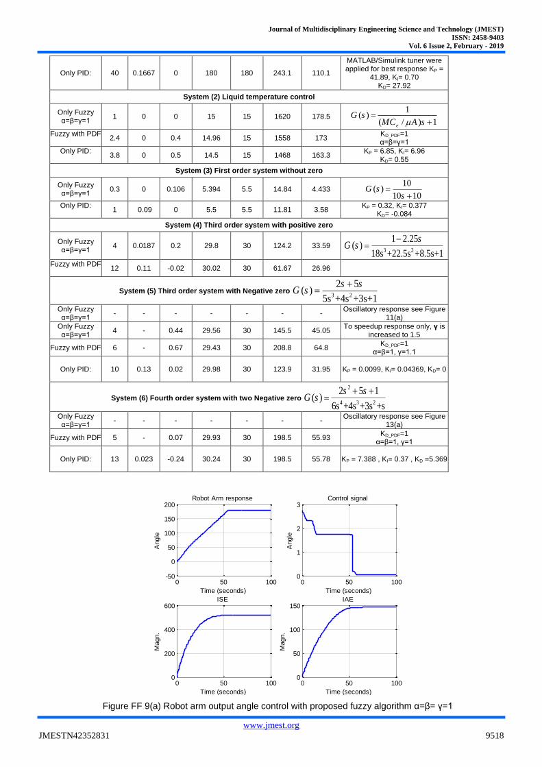
Only Fuzzy α=β=γ=1

12 0 1.2 178.8 180 516.5 147

Only Fuzzy with

α =β=1,γ=5 4 0 - 0.3 180.3 180 216.4 57.37

To speedup response only, parameter γ is increased to 5

Fuzzy with PDF

4 0 1.2 178.8 180 516.5 147 KD_PDF=1 α=β=γ=1

0 50 100 150-5

0

5

10

15

20

25

Time(s)

Outp

ut


= = =1

=0.1 , ==1

0 50 100 150-5

0

5

10

15

20

25

Time(s)

Outp

ut


= = =1

=0.1 , ==1

=, =1, =0.146

0 50 100 1500

1

2

3

4

5

6

Time(s)

Outp

ut

Response of sys. (No.4(TD)

0 10 20 30 40 50-5

0

5

10

15

Time(s)

Outp

ut


===1

=0.295, ==1

0 5 10

0

2

4

6

Time(s)

Outp

ut


=0.4, ==1

===1

0 10 20 30 40 500

2

4

6

Time(s)

Outp

ut


===1

=0.4, ==1



ISSN: 2458-9403


www.jmest.org

JMESTN42352831 9518

Only PID:

40 0.1667 0 180 180 243.1 110.1

MATLAB/Simulink tuner were applied for best response KP =

41.89, KI= 0.70 KD= 27.92

System (2) Liquid temperature control


1 0 0 15 15 1620 178.5 1

( )( / ) 1e

G sMC A s

Fuzzy with PDF

2.4 0 0.4 14.96 15 1558 173 KD_PDF=1 α=β=γ=1

Only PID:

3.8 0 0.5 14.5 15 1468 163.3 KP = 6.85, KI= 6.96

KD= 0.55

System (3) First order system without zero


0.3 0 0.106 5.394 5.5 14.84 4.433 10

( )10 10

G ss

Only PID:

1 0.09 0 5.5 5.5 11.81 3.58 KP = 0.32, KI= 0.377

KD= -0.084

System (4) Third order system with positive zero


4 0.0187 0.2 29.8 30 124.2 33.59 3 2

1 2.25( )

18s +22.5s +8.5s+1

sG s

Fuzzy with PDF

12 0.11 -0.02 30.02 30 61.67 26.96

System (5) Third order system with Negative zero 3 2

2 5( )

5s +4s +3s+1

s sG s


- - - - - - - Oscillatory response see Figure

11(a)


4 - 0.44 29.56 30 145.5 45.05 To speedup response only, γ is

increased to 1.5

Fuzzy with PDF 6 - 0.67 29.43 30 208.8 64.8 KD_PDF=1

α=β=1, γ=1.1

Only PID:

10 0.13 0.02 29.98 30 123.9 31.95 KP = 0.0099, KI= 0.04369, KD= 0

System (6) Fourth order system with two Negative zero

2

4 3 2

2 5 1( )

6s +4s +3s +s

s sG s


- - - - - - - Oscillatory response see Figure

13(a)

Fuzzy with PDF 5 - 0.07 29.93 30 198.5 55.93 KD_PDF=1

α=β=1, γ=1

Only PID:

13 0.023 -0.24 30.24 30 198.5 55.78 KP = 7.388 , KI= 0.37 , KD =5.369

Figure FF 9(a) Robot arm output angle control with proposed fuzzy algorithm α=β= γ=1

0 50 100-50

0

50

100

150

200

Time (seconds)

Angle

Robot Arm response

0 50 1000

1

2

3

Time (seconds)

Angle

Control signal

0 50 1000

200

400

600

Time (seconds)

Magn.

ISE

0 50 1000

50

100

150

Time (seconds)

Magn.

IAE



ISSN: 2458-9403


www.jmest.org

JMESTN42352831 9519

Figure FF9(b) Robot arm output angle control with proposed fuzzy algorithm α=β=1, and γ=5

Figure 10 Output Temperature control with proposed fuzzy α=β= γ=1

Figure 11(a) First order system without zero response with proposed fuzzy with α=β= γ=1

0 50 100-50

0

50

100

150

200

Time (seconds) A

ngle

Robot Arm with =5

0 50 100-10

-5

0

5

10

Time (seconds)

Angle

Control signal

0 50 1000

50

100

150

200

250

Time (seconds)

Magn.

ISE

0 50 1000

20

40

60

Time (seconds)

Magn.

IAE

0 5 10 15 200

5

10

15

20

Time (seconds)

T

Temperature control

0 5 10 15 20-6

-4

-2

0

2

4

Time (seconds)

Magn.

Control signal

0 5 10 15 200

500

1000

1500

2000

Time (seconds)

Magn.

ISE

0 5 10 15 200

50

100

150

200

Time (seconds)

Magn.

IAE

0 2 4 60

2

4

6

Time (seconds)

data

I order system

0 2 4 6-2

-1

0

1

2

3

Time (seconds)

data

Control signal

0 2 4 60

5

10

15

Time (seconds)

Magn.

ISE

0 2 4 60

1

2

3

4

5

Time (seconds)

data

IAE



ISSN: 2458-9403


www.jmest.org

JMESTN42352831 9520

Figure 11(a) Third order system with negative zero with proposed fuzzy with α=β= γ=1

Figure 12(a) Third order system with Positive zero with fuzzy α=β= γ=1

Figure 12(b) Third order system with negative zero with fuzzy α=β= 1 and γ=1.1 and with PDF control KPDF=1

0 20 40 600

10

20

30

40

Time (seconds)data

Third order system, Neg. Zero

0 20 40 60-4

-2

0

2

4

Time (seconds)

data

Control signal

0 20 40 600

50

100

150

200

Time (seconds)

Magn.

ISE

0 20 40 600

20

40

60

80

100

Time (seconds)

data

Time Series Plot:

0 20 40 60-10

0

10

20

30

40

Time (seconds)

data

III order system, Pos. Zero

0 20 40 60-2

-1

0

1

2

3

Time (seconds)data

Control signal

0 20 40 600

50

100

150

Time (seconds)

Magn.

ISE

0 20 40 600

10

20

30

40

Time (seconds)

data

Time Series Plot:

0 20 40 600

10

20

30

Time (seconds)

data


0 20 40 60-1

0

1

2

3

4

Time (seconds)

data

Control signal

0 20 40 600

50

100

150

200

250

Time (seconds)

Magn.

ISE

0 20 40 600

20

40

60

80

Time (seconds)

data

Time Series Plot:



ISSN: 2458-9403


www.jmest.org

JMESTN42352831 9521

Figure 12(d) Third order system with negative zero with only PID

Figure 13(a) Fourth order system with two negative zero with fuzzy α=β= 1 and γ=1

Figure 13(b) Fourth order system with two negative zero with fuzzy α=β= 1 and γ=1 and with PDF control with KPDF=1

Figure 13(c) Fourth order system with two negative zero with only PID

Conclusion

A generalized, direct, simple and user-friendly fuzzy logic control algorithm design approach for designing fuzzy logic based control algorithm applicable to control a variety of systems is presented. By defining ranges for universes of discourse of the two inputs and output between [-1,1], and defining the value of control unit operating voltage. To further adjust resulted response, two options are proposed; first is using three introduced soft tuning parameters with soft tuning ranges and effects. Second is by adding pseudo-derivative feedback control.

The proposed fuzzy control algorithm is simulated and tested to control a wide range of different systems, simulation results showed applicability of proposed design to result in acceptable stability and medium fastness of response. The following suggested steps can be followed to apply controller with proposed fuzzy control algorithm:

(1) Set the Vin equal to control unit operating voltage (e.g. 5.5 for microcontroller).

(2) Sensor with output voltage ± 5Vdc is connected to control unit.

0 20 40 600

10

20

30

40

Time (seconds)data


0 20 40 600

0.5

1

1.5

Time (seconds)

data

Control signal

0 10 20 30 400

20

40

60

80

Time (seconds)

data

IV order system, 2 Neg. Zero

0 10 20 30 40-4

-2

0

2

4

6

Time (seconds)data

Control signal

0 10 20 30 400

100

200

300

400

Time (seconds)

Magn.

ISE

0 10 20 30 400

20

40

60

80

100

Time (seconds)

data

Time Series Plot:

0 20 40 600

10

20

30

Time (seconds)

data


0 20 40 60-2

-1

0

1

2

3

Time (seconds)

data

Control signal

0 20 40 600

50

100

150

200

Time (seconds)

Magn.

ISE

0 20 40 600

20

40

60

Time (seconds)

data

Time Series Plot:

0 20 40 600

10

20

30

40

Time (seconds)

data


0 20 40 60-0.1

0

0.1

0.2

0.3

0.4

Time (seconds)

data

Control signal

0 20 40 600

50

100

150

200

Time (seconds)

Magn.

ISE

0 20 40 600

20

40

60

Time (seconds)

data

Time Series Plot:



ISSN: 2458-9403


www.jmest.org

JMESTN42352831 9522

(3) Output control signal from control unit is connected to drive circuit, that will drive the load.

(5) Run the system, with (α=β=γ=1). If the resulted response is not in desired acceptable range, then to further improve response consider steps (6), (7)

(5) To speedup resulted response, increase the output parameter (γ) (Recommended to increase by 0.5).

(6) To reducing error, overshoot and oscillation in resulted response, Decrease parameter (β). (Recommended: to decrease by 0.1) or (to reduce/remove overshoot, an initial (β) value is to set (β=2*PO%) or (PDF control can be switched on)

The proposed fuzzy algorithm showed shortage for controlling systems with time delay and first order systems with time constant less than 1. As future work; Further sharpening of the proposed algorithm is to be accomplished, as well as, to be applicable with other types of fuzzy control. For the output variable u, singleton membership functions are to be applied, defined and tested

References

[1] Farhan A. Salem, Ahmad A. Mahfouz 'Mechatronics Design And Implementation Education-Oriented Methodology; A Proposed Approach' Journal of Multidisciplinary Engineering Science and Technology Volume. 1 , Issue. 03 , October – 2014.

[2] Report of the Task Force on Intelligent Control IEEE Control Systems Society Panos Antsaklis, Chair, 1993.

[3] Altas I. H, 1998, The Effects of Fuzziness in Fuzzy Logic Controllers, 2nd International Symposium on Intelligent Manufacturing Systems, August 6-7, Sakarya University, Sakarya, Turkey, pp.211-220.

[4] Nauck D. and Kruse R., 1993, A Fuzzy Neural Network Learning Fuzzy Control Rules and Membership Functions by Fuzzy Error Backpropagation, Proc. IEEE Int. Conf. Neural Networks ICNN'93, San Francisco, Mar. 28 - Apr. 1, pp. 1022-1027.

[5] Herrera F., Lozano M., and Verdegay J. L., 1993, Generating Fuzzy Rules from Examples using Genetic Algorithms, Dept. of Computer Science and Artificial Intelligence, Technical Report #DECSAI-93115, October.

[6] Klawonn F. and Keller A., 1997, Fuzzy Clustering and Fuzzy Rules. Proc. 7th Intern. Fuzzy Systems Association World Congress(IFSA'97) Vol. I, Academia, Prague, pp.193-198.

[7] I. H. Altas and A. M. Sharaf, “A Generalized Direct Approach for Designing Fuzzy Logic Controllers in Matlab/Simulink GUI Environment”, Accepted for publication in International Journal of Information Technology and Intelligent Computing, Int. J. IT&IC no.4 vol.1.

[8] Zadeh L.A., Fuzzy sets, Information and Control, vol. 8, pp. 338–353, 1965

[9] Robert H. Bishop , Mechatronics: an introduction. CRC, Taylor & Francis, 2006

[10] Saban Çetin, Ali Volkan Akkaya, Simulation and Hybrid Fuzzy- PID control for positioning of a hydraulic system,” Nonlinear Dynamics, vol. 61, no. 3, pp. 465–476, 2010.

[11] Engin Yesil, Müjde Güzelkaya, Ibrahim Eksin, Fuzzy PID controllers: An overview, researchgate, 2003 (https://www.researchgate.net/publication/255567860)

[12] He, S. Z., Shaoua, T. D., Xu, F. L., 1993. Fuzzy self-tuning of PID. Fuzzy Sets and Systems (56), 37-46.

[13] Zhao, Z. Y., Tomizuka, M., Isaka, S., 1993. Fuzzy gain scheduling of PID controllers. IEEE Trans on Systems, Man, and Cybernetics 23(5), 1392-1398.

[14] Saban Çetin · Ali Volkan Akkaya, Simulation and Hybrid Fuzzy- PID control for positioning of a hydraulic system,” Nonlinear Dynamics, vol. 61, no. 3, pp. 465–476, 2010.

[15]Tanaka, K.: Introduction to Fuzzy Logic for Engineering Application. Springer, New York (1996). ISBN 0-387-94807

[16]Passino, K.M., Yurkovich, S.: Fuzzy Control. Addison– Wesley/Longman, Reading/Harlou (1998).

[17]Richard M. Phelan, Automatic Control Systems, Cornell University Press, Ithaca, New York, 1977 .

[18]Mike Borrello,'' Controls, Modeling and Simulation '' http://www. Stablesimulations.com

[19]Farhan A. Salem, Controllers and Control Algorithms: Selection and Time Domain Design Techniques Applied in Mechatronics Systems Design, International Journal of Engineering Sciences, 2(5) May 2013, Pages: 160-190


new efficient, simple and user friendly artificial fuzzy ... · applications. the fuzzy logic...

Documents