New Development in Coastal Ocean Analysis and Prediction

Peter C. ChuNaval Postgraduate SchoolMonterey, CA 93943, USA

Coastal Model

Major Problems in Coastal Modeling

(1) Discretization(2) Sigma Error(3) High-Order Scheme(4) POM Capability(5) Velocity Data Assimilation (6) Predictability

(1) Discretization

Diversity in Discretization

Finite DifferencesZ – coordinate (MOM, …)σ - coordinate (POM, COHERENS, etc…)s- coordinate (SCRUM, ROMS …)Layered/Isopycnal coordinates (NLOM, MICOM, …)

Finite Elements

Z-Coordiante

Note “staircase” topography representation, normally with no-slip conditions

Problems of the “Staircase Presentation”

Difficult in simulating coastal flow.

Example: Japan/East Sea (JES) Simulation (Kim and Yoon, 1998 JO)

JES Circulation Model Using MOM(Kim & Yoon, 1998)

1/6 deg resolution19 vertical levelMonthly mean wind stress (Na et al. 1992)Monthly mean heat flux (Haney type)

Problem in Simulating Coastal Currents

Model Observation

Layered/Isopycnal CoordinatesPro

Horizontal mixing is exactly along the surfaces of constant potential density

Avoids inconsistencies between vertical and horizontal transport terms

ConIt requires an evident layered structure (not suitable for shelf circulation

Some difficulty in modeling detrainment of ocean mixed layer

Layered/Isopycnal Coordinates

(Metzger andHurlburt 1996, JGR)1/8o, 6 layer with realistic bottom topographyNot applicable to simulating shelf circulation

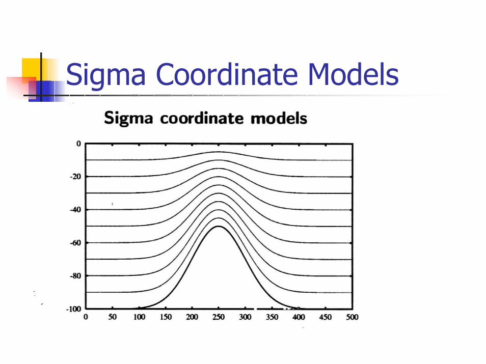
Sigma Coordinate Models

Sigma CoordinatesPro

Realistic Bottom Topography

Applicable to Shelf and Estuarine Circulation

ConHorizontal Pressure gradient ErrorHigh Vertical Resolution in Shallow Water (Shelf) and Low Resolution in Deep Water

Horizontal Diffusion

The second and fourth terms in the righthand side are generally ignored.

(2) Sigma Error

Pressure Gradient Error

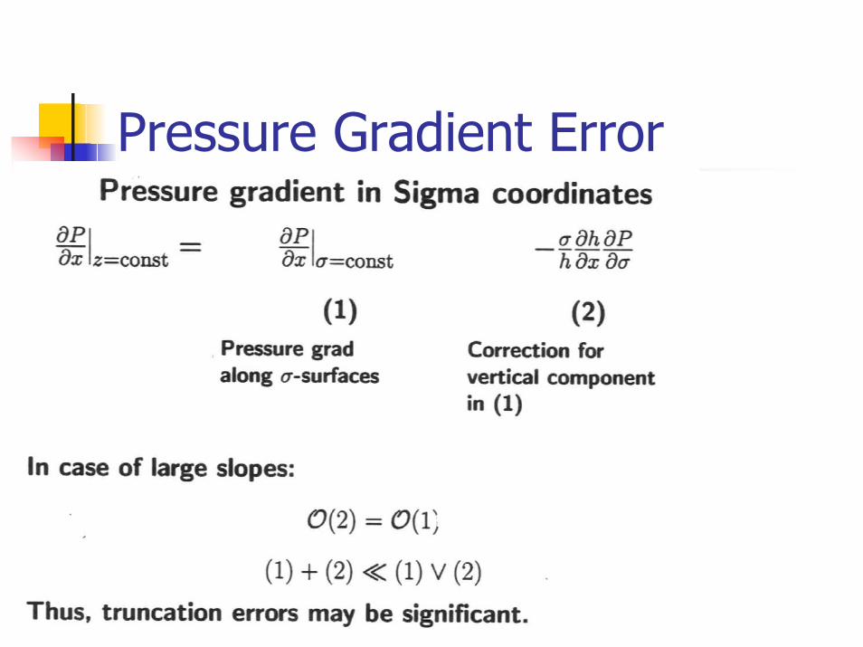
Pressure Gradient Error

Seamount Test Case

Two Kinds of Sigma Errors(Mellor et al. 1998, JTECH)

First Kind (SEFK):Horizontal Density GradientOscillatory Decaying

Second Kind (SESF)Vorticity Error

Reduction of Sigma Error

Smoothing topographySubtracting horizontally averaged density fieldUsing generalized topography-following coordinate system (e.g., S-coordinates in ROMS)Using high-order difference schemes

S-CoordinateGeneralized Topography-Following Coordinates (Song & Haidvogel, 1994)

Error Analysis (S-Coordinate)

Error Evolution (S-coordinate)

Radius of Seamount: r1 = 40 km, r2 =80 km

High-Order SchemesOrdinary Five-Point Sixth-Order Scheme (Chu and Fan, 1997 JPO)Three-Point Sixth-Order Combined Compact Difference (CCD) Scheme (Chu and Fan, 1998 JCP)Three-Point Sixth-Order Nonuniform CCD Scheme (Chu and Fan, 1999, JCP)Three-Point Sixth-Order Staggered CCD Scheme (Chu and Fan, 2000, Math. & Comp. Modeling)Accuracy Progressive Sixth-Order Scheme (Chu and Fan, 2001, JTECH) Finite Volume Model (Chu and Fan, 2002)

(3) Difference Schemes

Why do we need high-order schemes?

(1) Most ocean circulation models are hydrostatic.

(2) If keeping the same physics, the grid space (∆x) should be larger than certain criterion such that the aspect ratio

δ = H/ ∆x << 1

A Hidden Problem in Second Order Central Difference Scheme

Both Φ’ and Φ’’ are not continuous at each grid point. This may cause some problems.

Local Hermitian Polynomials

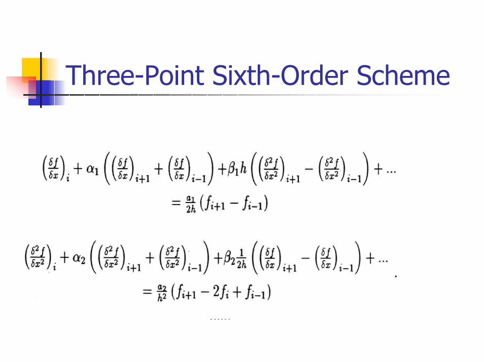
Three-Point Sixth-Order Scheme

Three-Point Sixth Order CCD Schemes

Existence of Global Hermitian PolynomialsFirst Derivative Continuous

Second Derivative Continuous

Error Reduction Using CCD Schemes (Seamount)

Rotating Cone for Testing Various Schemes

Accuracy Comparison

(4) POM Capability

Chu et al 2001, JTECH

Evaluation of POM Using the South China Sea Monsoon Experiment (SCSMEX) Data

IOP (April – June 1998)

T-S Diagram from SCSMEX Observations

Two Step Initialization of POM(1) Spin-up

Initial conditions: annual mean (T,S) + zero velocityClimatological annual mean winds + Restoring type thermohaline flux (2 years)

(2) Climatological ForcingMonthly mean winds + thermohaline fluxes from COADS (3 years) to 1 April

(3) The final state of the previous step is the initial state of the following step(4) Synoptic Forcing

NCEP Winds and Fluxes: April 1 to June 30, 1998 (3 Months)

Two Types of Model Integration

(1) MD1: Without Data Assimilation Hindcast Period: April-June 1998 (3 Months)

(2) MD2: With Daily SCSMEX-CTD Data Assimilation Hindcast Period:

May 1998: No data Assimilation in May June 1998: No data Assimilation in June

Skill-ScoreModel-Data Difference

Mean Square Error

Skill-Score (SS)

SS > 0, Model has capability

Scatter Diagrams Between Model and Observation (MD1)

Histograms of (Model – Obs) for MD1

RMS Error for MD1 (No Assimilation)

Bias for MD1 (No Assimilation)

Skill-Score for MD1 (No Assimilation)

Scatter Diagrams for MD2 (with Assimilation)

RMS Error for MD2 (with Assimilation)

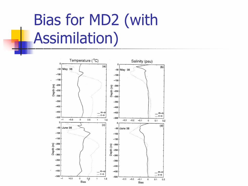
Bias for MD2 (with Assimilation)

Skill-Score for MD2 (with Assimilation)

Comments

(1) POM-SCS has synoptic flux forcing.(2) Without data assimilation, it has capability to predict temperature, but not salinity.(3) With data assimilation, it has capability to predict salinity.

(5) Velocity Data Assimilation

(Chu, et al 2002)

Can we get the velocity field from sparse and noisy data?

Reconstructed Currents from LATEX Drifting Buoy Data (Dec 15, 1993 – Mar

15, 1994)

Flow Decomposition

2 D Flow (Helmholtz)

3D Flow (Toroidal & Poloidal): Very popular in astrophysics

3D Incompressible Flow

When ± •u = 0We have

Flow Decomposition

±2 Ψ = - ζ, ζ is relative vorticity±2Φ = - w

Boundary Conditions

Basis Functions

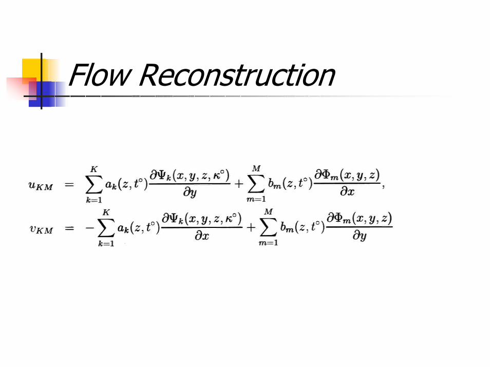
Flow Reconstruction

Several CommentsReconstruction is a useful tool for processing real-time velocity data with short duration and limited-area sampling.The scheme can handle highly noisy data.The scheme is model independent.The scheme can be used for velocity data assimilation.

6. Predictability

Model Valid Predictability Period (VPP)

ReferencesChu, P.C., L.M. Ivanov, T. M. Margolina, and O.V.Melnichenko, On probabilistic stability of an atmospheric model to various amplitude perturbations. Journal of the Atmospheric Sciences, 59, 2860-2873.Chu, P.C., L.M. Ivanov, and C.W. Fan, 2002: BackwardFokke-Planck equation for determining model valid prediction period. Journal of Geophysical Research, in press.Chu, P.C., L.M. Ivanov, L.H. Kantha, O.V. Melnichenko, and Y.A. Poberezhny, 2002: Power law decay in model predictability skill. Geophysical Research Letters, in press.

Question

How long is an ocean (or atmospheric) model valid once being integrated from its initial state?

Or what is the model valid prediction period (VPP)?

Atmospheric & Oceanic Model (Dynamic System with Stochastic Forcing)

d X/ dt = f(X, t) + q(t) X

Initial Condition: X(t0) = X0

Stochastic Forcing: <q(t)> = 0<q(t)q(t’)> = q2δ(t-t’)

Prediction Model

Y --- Prediction of X

Model: dY/dt = h(y, t)

Initial Condition: Y(t0) = Y0

Model Error

Z = X – Y

Initial: Z0 = X0 - Y0

Definition of VPP

VPP is defined as the time period when the prediction error first exceeds a pre-determined criterion (i.e., the tolerance level ε).

VPP

PredictabilityUsing VPP

One Scalar

Conventional

Error Growth

Z (t) = ?

For operational model, the vector Z may have many components

Uncertain Initial Error

The prediction is meaningful only if

VPP time period (t – t0)

Such that

Conditional Probability Density Function

Initial Error: Z0

(t – t0) Random Variable

Conditional PDF of (t – t0) with given Z0

P[(t – t0) |Z0]

Backward Fokker-Planck Equation

Backward Fokker-Planck Equation

Moments

Mean & Variance of VPP

Mean VPP: tau1

Variance of VPP:

tau2 – tau12

Linear Equations for Mean and Variance of VPP

For an autonomous dynamical systemd X/ dt = f(X) + q(t) X

Integration of [Backward F-P Eq. *

(t – t0), (t – t0)2] from t0 to infinity.

Example 1: One Dimensional Model (Nicolis 1992)

1D Dynamical System

Mean and Variance of VPP

Analytical Solutions

Dependence of tau1 & tau2 on Initial Condition Error ( )

Small Tolerance Error ( )

(1) Lyapunov Exponent: ( )(2) Stochastic Forcing (q 0):

Multiplicative White NoiseReducing the Lyapunov exponent (Stabilizing the dynamical system)

Dependence of Mean VPP on initial error and tolerance level

Dependence of Variance of VPP on initial error and tolerance level

Example 2: Multi-Dimensional Models: Power Decay Law in VPP

Model Error

Z = X – Y

Initial: Z0 = X0 - Y0

Error Mean and Variance

Error Mean

Error Variance

Exponential Error Growth

Classical Linear Theory

No Long-Term Predictability

Power Law

Long-Term Predictability May Occur

Gulf of Mexico Nowcast/Forecast System

University of Colorado Version of POM1/12o ResolutionReal-Time SSH Data (TOPEX, ESA ERS-1/2) AssimilatedReal Time SST Data (MCSST, NOAA AVHRR) AssimilatedSix Months Four-Times Daily Data From July 9, 1998 for Verification

Model Generated Velocity Vectors at 50 m on 00:00 July 9, 1998

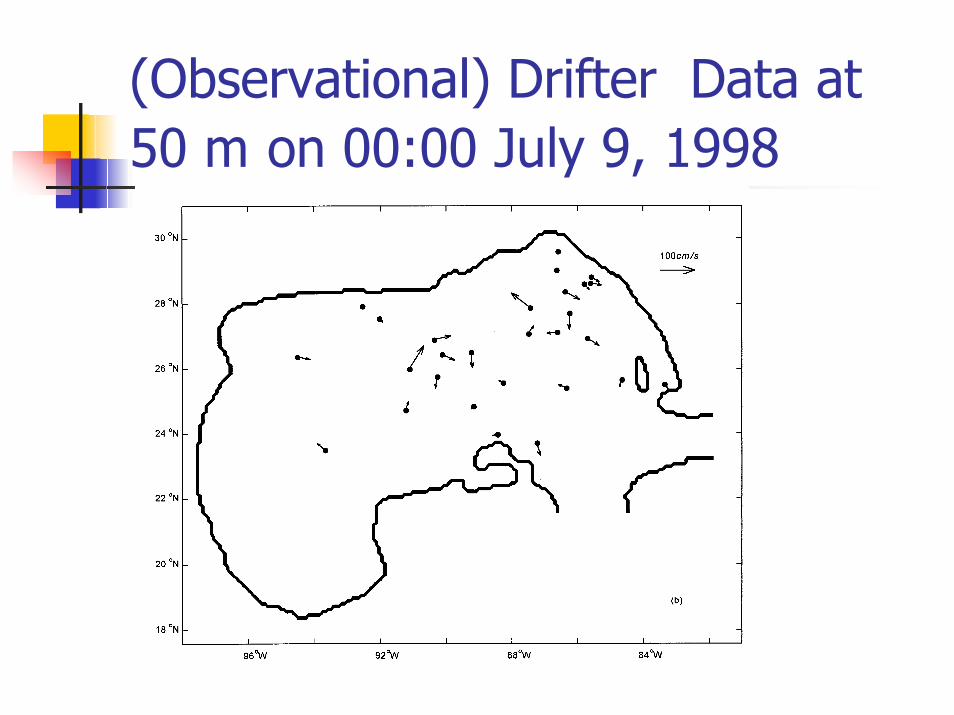
(Observational) Drifter Data at 50 m on 00:00 July 9, 1998

Reconstructed Drift Data at 50 m on 00:00 July 9, 1998 (Chu et al. 2002 a, b, JTECH)

Statistical Characteristics of VPP for zero initial error and 55 km tolerance level (Non-Gaussion)

Scaling behavior of the

mean error (L1) growth

for initial error levels:

(a) 0

(b) 2.2 km

(c) 22 km

Scaling behavior of the

Error variance (L2) growth

for initial error levels:

(a) 0

(b) 2.2 km

(c) 22 km

Probability Density Function of VPP calculated with different tolerance levels

Non-Gaussian distribution

with long tail toward large

values of VPP (Long-term

Predictability)

Conclusions

(1) VPP is an effective prediction skill measure (scalar).

(2) Backward Fokker-Planck equation is a useful tool for predictability study.

(3) Stochastic-Dynamic Modeling