new content 2012 mathematical studies sl 2012 mathematics

KEY New Content 2012 Mathematical studies SL 2012 Mathematics SL 2012 Mathematics HL 2012 Mathematics HL options Mathematics: applications & interpretation Mathematics: analysis & approaches SL Content Additional HL Content SL Content Additional HL Content

Topi

c 1:

Alg

ebra

SL 1.1*

Operations with numbers in the form x10ka where 1 10a≤ < and k is an integer.

AHL1.9

Laws of logarithms:

log log log

log log log

log logfor , , 0

a a a

a a a

ma a

xy x yx x yyx m x

a x y

= +

= −

=>

SL 1.1*

Operations with numbers in the form x10ka where 1 10a≤ < and k is an integer.

AHL 1.10

Counting principles, including permutations and combinations.

Extension of the binomial theorem to fractional and negative indices, ie., ( ) ,na b n+ ∈ .

SL1.2*

Arithmetic sequences and series.

Use of the formulae for the nth term and the sum of the first n terms of the sequence.

Use of sigma notation for sums of arithmetic sequences.

Applications.

Analysis, interpretation and prediction where a model is not perfectly arithmetic in real-life.

AHL 1.10

Simplifying expressions, both numerically and algebraically, involving rational exponents.

SL1.2*

Arithmetic sequences and series.


Use of sigma notation for sums of arithmetic sequences.

Applications.

Analysis, interpretation and prediction where a model is not perfectly arithmetic in real-life.

AHL 1.11

Partial fractions.

SL 1.3*

Geometric sequences and series.


Use of sigma notation for the sums of geometric sequences.

Applications.

AHL 1.11

The sum of infinite geometric sequences.

SL 1.3*

Geometric sequences and series.


Use of sigma notation for the sums of geometric sequences.

Applications.

AHL 1.12

Complex numbers: the number i , where 2i 1= −

Cartesian form iz a b= + ; the terms real part, imaginary part, conjugate, modulus and argument. The complex plane.

SL 1.4*

Financial applications of geometric sequences and series:

• Compound interest

• Annual depreciation

AHL 1.12

Complex numbers: the number i such that 2i 1= − .

Cartesian form: iz a b= + ; the terms real part, imaginary part, conjugate, modulus and argument.

Calculate sums, differences, products, quotients, by hand and with technology. Calculating powers of complex numbers, in Cartesian form, with technology.

The complex plane.

Complex numbers as solutions to quadratic equations of the form 2 0ax bx c+ + = , 0a ≠ , with real coefficients where 2 4 0b ac− <

SL 1.4*

Financial applications of geometric sequences and series:

• Compound interest

• Annual depreciation

AHL 1.13

Modulus-argument (polar) form:

( )cos i sinz r rcisθ θ θ= + = Euler form: iez r θ=

Sums, products and quotients in Cartesian, polar or Euler forms and their geometric interpretation.


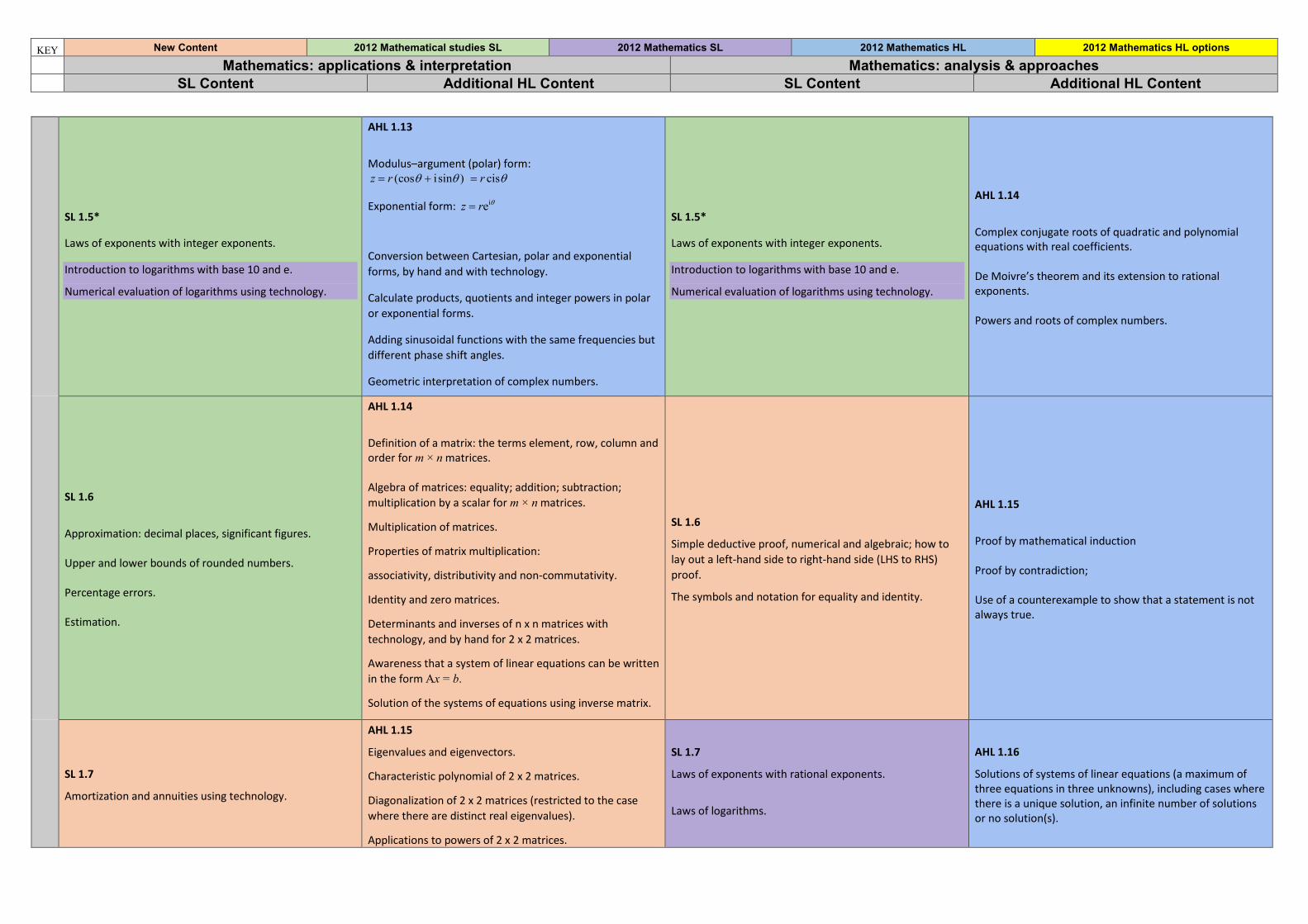
SL 1.5*

Laws of exponents with integer exponents.

Introduction to logarithms with base 10 and e.

Numerical evaluation of logarithms using technology.

AHL 1.13

Modulus–argument (polar) form:

cos isi( )n cis z r rθ θ θ= + =

Exponential form: iez r θ=

Conversion between Cartesian, polar and exponential forms, by hand and with technology.

Calculate products, quotients and integer powers in polar or exponential forms.

Adding sinusoidal functions with the same frequencies but different phase shift angles.

Geometric interpretation of complex numbers.

SL 1.5*

Laws of exponents with integer exponents.

Introduction to logarithms with base 10 and e.

Numerical evaluation of logarithms using technology.

AHL 1.14

Complex conjugate roots of quadratic and polynomial equations with real coefficients. De Moivre’s theorem and its extension to rational exponents. Powers and roots of complex numbers.

SL 1.6

Approximation: decimal places, significant figures. Upper and lower bounds of rounded numbers. Percentage errors. Estimation.

AHL 1.14

Definition of a matrix: the terms element, row, column and order for m × n matrices. Algebra of matrices: equality; addition; subtraction; multiplication by a scalar for m × n matrices.

Multiplication of matrices.

Properties of matrix multiplication:

associativity, distributivity and non-commutativity.

Identity and zero matrices.

Determinants and inverses of n x n matrices with technology, and by hand for 2 x 2 matrices.

Awareness that a system of linear equations can be written in the form Ax = b.

Solution of the systems of equations using inverse matrix.

SL 1.6

Simple deductive proof, numerical and algebraic; how to lay out a left-hand side to right-hand side (LHS to RHS) proof.

The symbols and notation for equality and identity.

AHL 1.15

Proof by mathematical induction Proof by contradiction; Use of a counterexample to show that a statement is not always true.

SL 1.7

Amortization and annuities using technology.

AHL 1.15

Eigenvalues and eigenvectors.

Characteristic polynomial of 2 x 2 matrices.

Diagonalization of 2 x 2 matrices (restricted to the case where there are distinct real eigenvalues).

Applications to powers of 2 x 2 matrices.

SL 1.7

Laws of exponents with rational exponents.

Laws of logarithms.

AHL 1.16

Solutions of systems of linear equations (a maximum of three equations in three unknowns), including cases where there is a unique solution, an infinite number of solutions or no solution(s).


log log log

log log log

log logfor , , 0

a a a

a a a

ma a

xy x yx x yyx m x

a x y

= +

= −

=>

Change of base of a logarithm.

logloglog

ba

b

xxa

= , for , , 0a b x >

Solving exponential equations, including using logarithms.

SL 1.8

Use technology to solve:

• Systems of linear equations in up to 3 variables

• Polynomial equations

SL 1.8

Sum of infinite convergent geometric sequences.

SL 1.9

The binomial theorem: expansion of ( ) ,na b n+ ∈

Use of Pascal’s triangle and Cnr .

Topi

c 2:

Fun

ctio

ns

SL 2.1*

Different forms of the equation of a straight line. Gradient; intercepts. Lines with gradients 1m and 2m . Parallel lines 1 2m m= . Perpendicular lines 1 2x 1m m = − .

AHL 2.7

Composite functions in context.

The notation ( )( ) ( ( ))f g x f g x=

Inverse function 1f − , including domain restriction.

Finding an inverse function.

SL 2.1*

Different forms of the equation of a straight line. Gradient; intercepts. Lines with gradients 1m and 2m . Parallel lines 1 2m m= . Perpendicular lines 1 2x 1m m = − .

AHL 2.12

Polynomial functions, their graphs and equations; zeros, roots and factors.

The factor and remainder theorems.

Sum and product of the roots of polynomial equations.

Fu

nctio

n no

tatio

n, e

g.

)n

.

SL 2.2*

Concept of a function, domain, range and graph. Function notation, eg. ( ), ( ), ( )f x v t C n . The concept of a function as a mathematical model. Informal concept that an inverse function reverses or undoes the effect of a function. Inverse function as a reflection in the line y = x and the notation 1( )f x− .

AHL2.8

Translations: ( ) ;y f x b= + ( )y f x a= −

Reflections: in the x axis ( )y pf x= , and in the y axis ( )y f x= −

Vertical stretch with scale factor p: ( )y pf x=

Horizontal stretch with scale factor 1q

: ( )y f qx=

Composite transformations.

SL 2.2*

Concept of a function, domain, range and graph. Function notation, eg. ( ), ( ), ( )f x v t C n . The concept of a function as a mathematical model. Informal concept that an inverse function reverses or undoes the effect of a function. Inverse function as a reflection in the line y = x and the notation 1( )f x− .

AHL 2.13

Rational functions of the form 2

2( ) , and ( )ax b ax bx cf x f xcx dx e dx e

+ + += =

+ + +


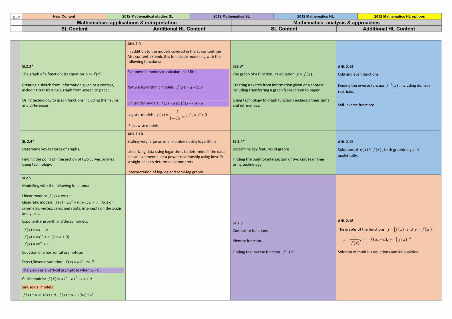
SL2.3*

The graph of a function; its equation ( )y f x= . Creating a sketch from information given or a context, including transferring a graph from screen to paper. Using technology to graph functions including their sums and differences.

AHL 2.9

In addition to the models covered in the SL content the AHL content extends this to include modelling with the following functions: Exponential models to calculate half-life;

Natural logarithmic models: ( ) lnf x a x= +

Sinusoidal models: ( ) sin ( ( ))f x a b x c d= − +

Logistic models: ( )1 e kx

Lf xC −=

+; , , 0L k C >

Piecewise models.

SL2.3*

The graph of a function; its equation ( )y f x= . Creating a sketch from information given or a context, including transferring a graph from screen to paper. Using technology to graph functions including their sums and differences.

AHL 2.14

Odd and even functions. Finding the inverse function 1( )f x− , including domain restriction.

Self-inverse functions.

SL 2.4*

Determine key features of graphs. Finding the point of intersection of two curves or lines using technology.

AHL 2.10

Scaling very large or small numbers using logarithms; Linearizing data using logarithms to determine if the data has an exponential or a power relationship using best-fit straight lines to determine parameters Interpretation of log-log and semi-log graphs.

SL 2.4*

Determine key features of graphs. Finding the point of intersection of two curves or lines using technology.

AHL 2.15

Solutions of ( ) ( )g x f x≥ , both graphically and analytically.

SL2.5

Modelling with the following functions: Linear models: ( )f x mx c= + . Quadratic models: 2( ) ; 0f x ax bx c a= + + ≠ . Axis of symmetry, vertex, zeros and roots, intercepts on the x-axis and y-axis.

Exponential growth and decay models:

( )( ) , (for 0)( ) e

x

x

rx

f x ka cf x ka c af x k c

−

= +

= + >

= +

Equation of a horizontal asymptote.

Direct/inverse variation: ( ) ,nf x ax n= ∈

The y-axis as a vertical asymptote when 0n < .

Cubic models: 3 2( )f x ax bx cx d= + + +

Sinusoidal models:

( ) sin ( ) , ( ) cos( )f x a bx d f x a bx d= + = +

SL 2.5

Composite functions Identity function. Finding the inverse function 1( )f x−

AHL 2.16

The graphs of the functions, ( )y f x= and ( )y f x= ,

[ ] 21 , ( ), ( )( )

y y f ax b y f xf x

= = + =

Solution of modulus equations and inequalities.


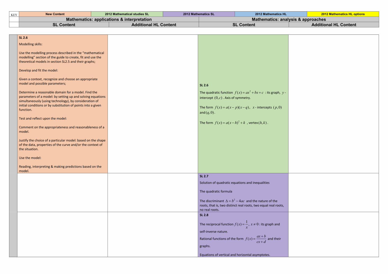
SL 2.6

Modelling skills: Use the modelling process described in the “mathematical modelling” section of the guide to create, fit and use the theoretical models in section SL2.5 and their graphs; Develop and fit the model: Given a context, recognize and choose an appropriate model and possible parameters; Determine a reasonable domain for a model. Find the parameters of a model: by setting up and solving equations simultaneously (using technology), by consideration of initial conditions or by substitution of points into a given function. Test and reflect upon the model: Comment on the appropriateness and reasonableness of a model. Justify the choice of a particular model: based on the shape of the data, properties of the curve and/or the context of the situation. Use the model: Reading, interpreting & making predictions based on the model.

SL 2.6

The quadratic function 2( )f x ax bx c= + + : its graph, y -intercept (0, )c . Axis of symmetry. The form ( ) ( )( )f x a x p x q= − − , x - intercepts ( ,0)p and ( ,0)q . The form 2( ) ( )f x a x h k= − + , vertex ( , )h k .

SL 2.7

Solution of quadratic equations and inequalities The quadratic formula The discriminant 2 4b ac∆ = − and the nature of the roots, that is, two distinct real roots, two equal real roots, no real roots.

SL 2.8

The reciprocal function1( ) , 0f x xx

= ≠ : its graph and

self-inverse nature.

Rational functions of the form ( ) ax bf xcx d

+=

+ and their

graphs. Equations of vertical and horizontal asymptotes.


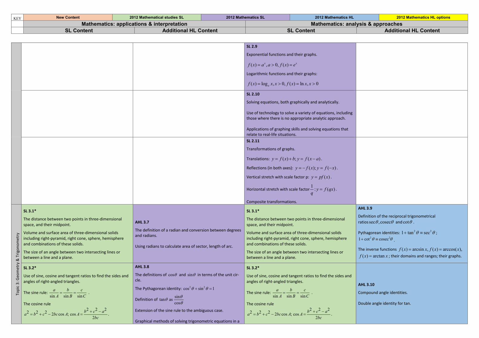
SL 2.9

Exponential functions and their graphs.

( ) , 0, ( )x xf x a a f x e= > =

Logarithmic functions and their graphs:

( ) log , 0, ( ) ln , 0af x x x f x x x= > = >

SL 2.10

Solving equations, both graphically and analytically. Use of technology to solve a variety of equations, including those where there is no appropriate analytic approach. Applications of graphing skills and solving equations that relate to real-life situations.

SL 2.11

Transformations of graphs.

Translations: ( ) ; ( )y f x b y f x a= + = − .

Reflections (in both axes): ( ); ( )y f x y f x= − = − .

Vertical stretch with scale factor p: ( )y pf x= .

Horizontal stretch with scale factor1 : ( )y f qxq

= .

Composite transformations.

Topi

c 3:

Geo

met

ry &

Trig

onom

etry

SL 3.1*

The distance between two points in three-dimensional space, and their midpoint.

Volume and surface area of three-dimensional solids including right-pyramid, right cone, sphere, hemisphere and combinations of these solids.

The size of an angle between two intersecting lines or between a line and a plane.

AHL 3.7

The definition of a radian and conversion between degrees and radians. Using radians to calculate area of sector, length of arc.

SL 3.1*

The distance between two points in three-dimensional space, and their midpoint.

Volume and surface area of three-dimensional solids including right-pyramid, right cone, sphere, hemisphere and combinations of these solids.

The size of an angle between two intersecting lines or between a line and a plane.

AHL 3.9

Definition of the reciprocal trigonometrical ratiossec ,cosecθ θ and cotθ .

Pythagorean identities: 2 21 tan secθ θ+ ≡ ; 2 21 cot cosecθ θ+ ≡ .

The inverse functions ( ) arcsin , ( ) arccos( ),f x x f x x= = ( ) arctanf x x= ; their domains and ranges; their graphs.

SL 3.2*

Use of sine, cosine and tangent ratios to find the sides and angles of right-angled triangles.

The sine rule: sin sin sin

a b cA B C= = .

The cosine rule

2 2 2 2 cos ;a b c bc A= + −2 2 2

cos2

b c aAbc

+ −= .

AHL 3.8

The definitions of cosθ and sinθ in terms of the unit cir-cle.

The Pythagorean identity: 2 2cos sin 1θ θ+ =

Definition of sintan ascos

θθθ

Extension of the sine rule to the ambiguous case. Graphical methods of solving trigonometric equations in a

SL 3.2*

Use of sine, cosine and tangent ratios to find the sides and angles of right-angled triangles.

The sine rule: sin sin sin

a b cA B C= = .

The cosine rule

2 2 2 2 cos ;a b c bc A= + −2 2 2

cos2

b c aAbc

+ −= .

AHL 3.10

Compound angle identities. Double angle identity for tan.


Area of a triangle as 1 sin2

ab C . finite interval.

Area of a triangle as 1 sin

2ab C .

SL 3.3* Applications of right and non-right-angled trigonometry including Pythagoras.

Angles of elevation and depression.

Construction of labelled diagrams from written statements.

AHL 3.9

Geometric transformations of points in two dimensions using matrices: reflections, horizontal and vertical stretches, enlargements, translations and rotations. Compositions of the above transformations.

Geometric interpretation of the determinant of a transformation matrix.

SL 3.3* Applications of right and non-right-angled trigonometry including Pythagoras.

Angles of elevation and depression.

Construction of labelled diagrams from written statements.

AHL 3.11

Relationships between trigonometric functions and the symmetry properties of their graphs.

SL 3.4 The circle: length of an arc; area of a sector.

AHL 3.10

Concept of a vector and a scalar.

Representation of vectors using directed line segments.

Unit vectors; base vectors i, j, k.

Components of a vector; column representation;

The zero vector 0, the vector -v .

Position vectors OA→

= a .

AB OB OA→ → →

= − = −b a Rescaling and normalizing vectors.

SL 3.4

The circle: radian measure of angles; length of an arc; area of a sector.

AHL 3.12

Concept of a vector; position vectors; displacement vectors.

Representation of vectors using directed line segments.

Base vectors i, j, k.

Components of a vector: .

Algebraic and geometric approaches to the following:

• the sum and difference of two vectors; • the zero vector 0 , the vector −v ; • multiplication by a scalar, kv , parallel vectors;

• magnitude of a vector, v ; unit vectors, vv

;

• position vectors OA , OB→ →

= =a b

• displacement vector AB→

= −b a Proofs of geometrical properties using vectors.

SL 3.5 Equations of perpendicular bisectors.

AHL 3.11 Vector equation of a line in two and three dimensions:

λ= +r a b , where b is a direction vector of the line.

SL 3.5 Definition of cos ,sinθ θ in terms of the unit circle.

Definition of tanθ as sincos

θθ

.

Exact values of trigonometric ratios of 0, , , ,6 4 3 2π π π π

and

their multiples.

Extension of the sine rule to the ambiguous case.

AHL 3.13 The definition of the scalar product of two vectors. The angle between two vectors Perpendicular vectors; parallel vectors.


SL 3.6 Voronoi diagrams; sites, vertices, edge, cells. Addition of a site to an existing Voronoi diagram. Nearest neighbour interpolation. Applications including the “toxic waste dump” problem.

AHL 3.12 Vector applications to kinematics Modelling linear motion with constant velocity in two and three dimensions. Motion with variable velocity in two dimensions.

SL 3.6 The Pythagorean identity 2 2cos sin 1θ θ+ = .

Double angle identities for sine and cosine.

The relationship between trigonometric ratios.

AHL 3.14

Vector equation of a line in two and three dimensions: λ= +r a b .

The angle between two lines.

Simple applications to kinematics.

AHL 3.13 Definition and calculation of the scalar product of two vectors The angle between two vectors; the acute angle between two lines. Definition and calculation of the vector product of two vectors. Geometric interpretation of ×v w . Components of vectors.

SL 3.7 The circular functions sin , cos and tanx x x ; amplitude, their periodic nature, and their graphs

Composite functions of the form ( )( ) sin ( )f x a b x c d= + + .

Transformations.

Real-life contexts.

AHL 3.15 Coincident, parallel, intersecting and skew lines, distinguishing between these cases. Points of intersection.

AHL 3.14 Graph theory: Graphs, vertices, edges, adjacent vertices, adjacent edges, degree of a vertex Simple graphs; complete graphs; weighted graphs. Directed graphs; indegree and outdegree of the vertices of a directed graph. Subgraphs; trees

SL 3.8 Solving trigonometric equations in a finite interval, both graphically and analytically. Equations leading to quadratic equations in

sin ,cos ,x x or tan x .

AHL 3.16 The definition of the vector product of two vectors. Properties of the vector product. Geometric interpretation of xv w .

AHL 3.15 • Adjacency matrices • Walks • Number of k-length walks (or less than k-length walks)

between two vertices. • Weighted adjacency tables • Construction of the transition matrix for strongly-

connected, undirected or directed graphs.

AHL 3.17 Vector equations of a plane: λ µ= + +r a b c , where b and c are non-parallel vectors within the plane.

⋅ = ⋅r n a n , where n is a normal to the plane and a is the position vector of a point on the plane.

Cartesian equation of a plane ax by cz d+ + = .

AHL 3.16 • Tree and cycle algorithms with undirected graphs • Walks, trails, paths, circuits, cycles • Eulerian trails and circuits • Hamiltonian paths and cycles • Minimum spanning tree (MST) graph algorithms:

Kruskal’s and Prim’s algorithms for finding minimum spanning trees.

• Chinese postman problem and algorithm for solution, to determine the shortest route around a weighted graph with up to four odd vertices, going along each edge at least once.

• Travelling salesman problem to determine the

AHL 3.18 Intersections of: a line with a plane, two planes, three planes. Angle between: a line and a plane, two planes.


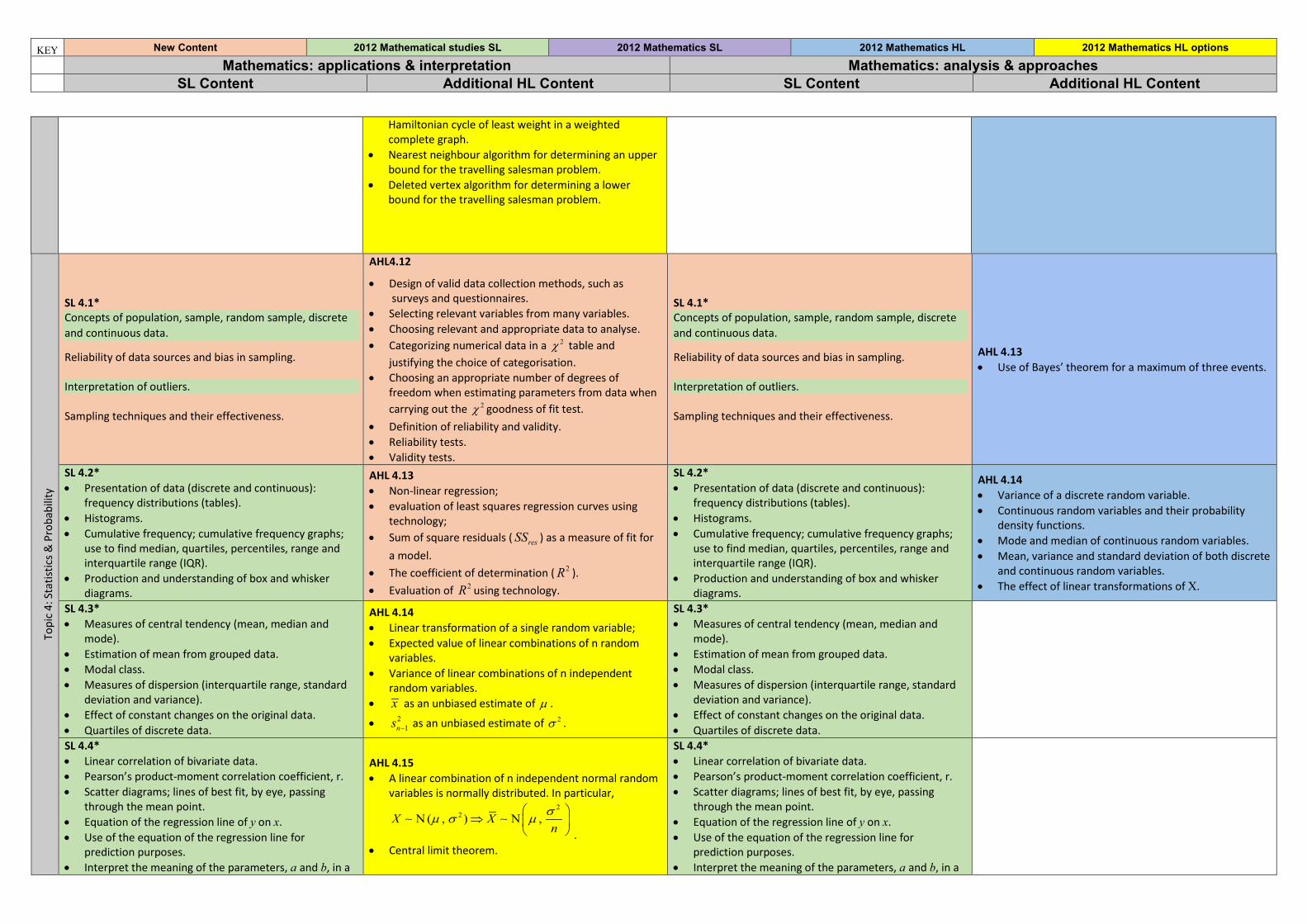
Hamiltonian cycle of least weight in a weighted complete graph.

• Nearest neighbour algorithm for determining an upper bound for the travelling salesman problem.

• Deleted vertex algorithm for determining a lower bound for the travelling salesman problem.

Topi

c 4:

Sta

tistic

s & P

roba

bilit

y

SL 4.1* Concepts of population, sample, random sample, discrete and continuous data.

Reliability of data sources and bias in sampling. Interpretation of outliers. Sampling techniques and their effectiveness.

AHL4.12

• Design of valid data collection methods, such as surveys and questionnaires.

• Selecting relevant variables from many variables. • Choosing relevant and appropriate data to analyse. • Categorizing numerical data in a 2χ table and

justifying the choice of categorisation. • Choosing an appropriate number of degrees of

freedom when estimating parameters from data when carrying out the 2χ goodness of fit test.

• Definition of reliability and validity. • Reliability tests. • Validity tests.

SL 4.1* Concepts of population, sample, random sample, discrete and continuous data.

Reliability of data sources and bias in sampling. Interpretation of outliers. Sampling techniques and their effectiveness.

AHL 4.13 • Use of Bayes’ theorem for a maximum of three events.

SL 4.2* • Presentation of data (discrete and continuous):

frequency distributions (tables). • Histograms. • Cumulative frequency; cumulative frequency graphs;

use to find median, quartiles, percentiles, range and interquartile range (IQR).

• Production and understanding of box and whisker diagrams.

AHL 4.13 • Non-linear regression; • evaluation of least squares regression curves using

technology; • Sum of square residuals ( resSS ) as a measure of fit for

a model. • The coefficient of determination ( 2R ). • Evaluation of 2R using technology.

SL 4.2* • Presentation of data (discrete and continuous):

frequency distributions (tables). • Histograms. • Cumulative frequency; cumulative frequency graphs;

use to find median, quartiles, percentiles, range and interquartile range (IQR).

• Production and understanding of box and whisker diagrams.

AHL 4.14 • Variance of a discrete random variable. • Continuous random variables and their probability

density functions. • Mode and median of continuous random variables. • Mean, variance and standard deviation of both discrete

and continuous random variables. • The effect of linear transformations of X.

SL 4.3* • Measures of central tendency (mean, median and

mode). • Estimation of mean from grouped data. • Modal class. • Measures of dispersion (interquartile range, standard

deviation and variance). • Effect of constant changes on the original data. • Quartiles of discrete data.

AHL 4.14 • Linear transformation of a single random variable; • Expected value of linear combinations of n random

variables. • Variance of linear combinations of n independent

random variables. • x as an unbiased estimate of µ .

• 21ns − as an unbiased estimate of 2σ .

SL 4.3* • Measures of central tendency (mean, median and

mode). • Estimation of mean from grouped data. • Modal class. • Measures of dispersion (interquartile range, standard

deviation and variance). • Effect of constant changes on the original data. • Quartiles of discrete data.

SL 4.4* • Linear correlation of bivariate data. • Pearson’s product-moment correlation coefficient, r. • Scatter diagrams; lines of best fit, by eye, passing

through the mean point. • Equation of the regression line of y on x. • Use of the equation of the regression line for

prediction purposes. • Interpret the meaning of the parameters, a and b, in a

AHL 4.15 • A linear combination of n independent normal random

variables is normally distributed. In particular, 2

2N ( , ) N ,X Xnσµ σ µ

⇒

. • Central limit theorem.

SL 4.4* • Linear correlation of bivariate data. • Pearson’s product-moment correlation coefficient, r. • Scatter diagrams; lines of best fit, by eye, passing

through the mean point. • Equation of the regression line of y on x. • Use of the equation of the regression line for

prediction purposes. • Interpret the meaning of the parameters, a and b, in a


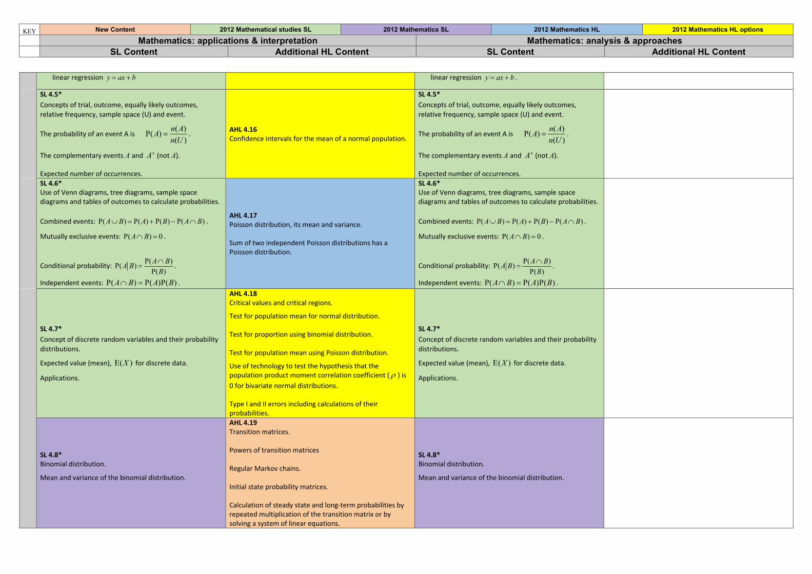
linear regression y ax b= + linear regression y ax b= + .

SL 4.5* Concepts of trial, outcome, equally likely outcomes, relative frequency, sample space (U) and event.

The probability of an event A is ( )P( )( )

n AAn U

= .

The complementary events A and 'A (not A). Expected number of occurrences.

AHL 4.16 Confidence intervals for the mean of a normal population.

SL 4.5* Concepts of trial, outcome, equally likely outcomes, relative frequency, sample space (U) and event.

The probability of an event A is ( )P( )( )

n AAn U

= .

The complementary events A and 'A (not A). Expected number of occurrences.

SL 4.6* Use of Venn diagrams, tree diagrams, sample space diagrams and tables of outcomes to calculate probabilities. Combined events: P( ) P( ) P( ) P( )A B A B A B∪ = + − ∩ .

Mutually exclusive events: P( ) 0A B∩ = .

Conditional probability: P( )P( )P( )A BA B

B∩

= .

Independent events: P( ) P( )P( )A B A B∩ = .

AHL 4.17 Poisson distribution, its mean and variance. Sum of two independent Poisson distributions has a Poisson distribution.

SL 4.6* Use of Venn diagrams, tree diagrams, sample space diagrams and tables of outcomes to calculate probabilities. Combined events: P( ) P( ) P( ) P( )A B A B A B∪ = + − ∩ .

Mutually exclusive events: P( ) 0A B∩ = .

Conditional probability: P( )P( )P( )A BA B

B∩

= .

Independent events: P( ) P( )P( )A B A B∩ = .

SL 4.7* Concept of discrete random variables and their probability distributions.

Expected value (mean), E( )X for discrete data.

Applications.

AHL 4.18 Critical values and critical regions.

Test for population mean for normal distribution. Test for proportion using binomial distribution. Test for population mean using Poisson distribution.

Use of technology to test the hypothesis that the population product moment correlation coefficient ( ρ ) is 0 for bivariate normal distributions. Type I and II errors including calculations of their probabilities.

SL 4.7* Concept of discrete random variables and their probability distributions.

Expected value (mean), E( )X for discrete data.

Applications.

SL 4.8* Binomial distribution.

Mean and variance of the binomial distribution.

AHL 4.19 Transition matrices. Powers of transition matrices Regular Markov chains. Initial state probability matrices. Calculation of steady state and long-term probabilities by repeated multiplication of the transition matrix or by solving a system of linear equations.

SL 4.8* Binomial distribution.

Mean and variance of the binomial distribution.


SL 4.9* The normal distribution and curve.

Properties of the normal distribution.

Diagrammatic representation. Normal probability calculations. Inverse normal calculations.

SL 4.9* The normal distribution and curve.

Properties of the normal distribution.

Diagrammatic representation. Normal probability calculations. Inverse normal calculations.

SL 4.10 Spearman’s rank correlation coefficient, rs.

Awareness of the appropriateness and limitations of Pearson’s product moment correlation coefficient and Spearman’s rank correlation coefficient, and the effect of outliers on each.

SL 4.10 Equation of the regression line of x on y.

Use of this equation for prediction purposes.

SL 4.11 Formulation of null and alternative hypotheses, H0 and H1.

Significance levels.

p-values.;

Expected and observed frequencies.

The test for independence: contingency tables, degrees of freedom, critical value.

The goodness of fit test.

The t-test.

Use of the p-value to compare the means of two popula-tions.

Using one-tailed and two-tailed tests.

SL 4.11 Formal definition and use of the formulae:

P( )P( )P( )A BA B

B∩

= for conditional probabilities, and

P( ) ( ) ( ')A B P A P A B= = for independent events.

SL 4.12 Standardization of normal variables (z-values).

Inverse normal calculations where mean and standard deviation are unknown.

Topi

c 5:

Cal

culu

s SL 5.1* Introduction to the concept of a limit.

Derivative interpreted as gradient function and as rate of change.

AHL 5.9 The derivatives of sin x, cos x, tan x, ex, ln x, xn where n∈ .

The chain rule, product rule and quotient rules.

Related rates of change.

SL 5.1* Introduction to the concept of a limit.

Derivative interpreted as gradient function and as rate of change.

AHL 5.12 Informal understanding of continuity and differentiability of a function at a point. Understanding of limits (convergence and divergence). Definition of derivative from first principles


0

( ) ( )( ) limh

f x h f xf xh→

+ −′ = .

Higher derivatives.

SL 5.2* Increasing and decreasing functions.

Graphical interpretation of ( ) 0, ( ) 0, ( ) 0.f x f x f x′ ′ ′> = <

AHL 5.10 The second derivative. Use of second derivative test to distinguish between a maximum and a minimum point.

SL 5.2* Increasing and decreasing functions.

Graphical interpretation of ( ) 0, ( ) 0, ( ) 0.f x f x f x′ ′ ′> = <

AHL 5.13

The evaluation of limits of the form ( )lim( )x a

f xg x→

and

( )lim( )x

f xg x→∞

using l’Hôpital’s Rule.

Repeated use of l’Hôpital’s rule.

SL 5.3* Derivative of ' 1( ) ( )n nf x ax is f x anx −= = , n∈

The derivative of functions of the form: 1( ) ....,n nf x ax bx −= + + where n∈ .

AHL 5.11 Definite and indefinite integration of nx where n∈ ,

including n = -1 , sin x, cos x, 2

1cos x

and ex.

Integration by inspection, or substitution of the form

( ( )) ( )f g x g x dx′∫ .

SL 5.3* Derivative of ' 1( ) ( )n nf x ax is f x anx −= = , n∈

The derivative of functions of the form: 1( ) ....,n nf x ax bx −= + + where n∈ .

AHL 5.14 Implicit differentiation. Related rates of change. Optimisation problems.

SL 5.4* Tangents and normals at a given point, and their equations.

AHL 5.12 Area of the region enclosed by a curve and the x -axis or y -axis in a given interval.

volumes of revolution about the x -axis or y -axis.

SL 5.4* Tangents and normals at a given point, and their equations.

AHL 5.15

Derivatives of: tan , sec , cosec , cot , , log ,arcsin , arccos , arctan

xax x x x a x

x x x

Indefinite integrals of the derivatives of any of the above functions.

The composites of any of these with a linear function.

Use of partial fractions to rearrange the integrand. SL 5.5* Introduction to integration as anti-differentiation of functions of the form 1( ) ....,n nf x ax bx −= + + where

, 1n n∈ ≠ − .

Definite integrals using technology.

Areas between a curve ( )y f x= and the x-axis, where ( ) 0f x > .

Anti-differentiation with a boundary condition to determine the constant term.

AHL 5.13 Kinematic problems involving displacement s , velocity v and acceleration a .

SL 5.5* Introduction to integration as anti-differentiation of functions of the form 1( ) ....,n nf x ax bx −= + + where

, 1n n∈ ≠ − .

Definite integrals using technology.

Areas between a curve ( )y f x= and the x-axis, where ( ) 0f x > .

Anti-differentiation with a boundary condition to determine the constant term.

AHL 5.16 Integration by substitution. Integration by parts. Repeated integration by parts.

SL 5.6 Values of x where the gradient of a curve is zero.

Solution of '( ) 0f x = .

Local maximum and minimum points.

AHL 5.14 Setting up a model/differential equation from a context. Solving by separation of variables

SL 5.6 Derivative of ( ),sin ,cos ,n xx n x x e∈ and ln x .

Differentiation of a sum and a multiple of these functions.

The chain rule for composite functions.

The product and quotient rules.

AHL 5.17 Area of the region enclosed by a curve and the y -axis in a given interval. Volumes of revolution about the x -axis or y -axis.


SL 5.7 Optimization problems in context.

AHL 5.15 Slope fields and their diagrams.

SL 5.7 The second derivative.

Graphical behaviour of functions, including the relationship between the graphs of ,f f ′ and f ′′ .

AHL 5.18 First order differential equations.

Numerical solution of d ( , )dy f x yx= using Euler’s method.

Variables separable.

Homogeneous differential equation dy yfdx x

=

using

the substitution y vx= .

Solution of ( ) ( )y P x y Q x′ + = , using the integrating factor.

SL 5.8 Approximating areas using the trapezoidal rule.

AHL 5.16 Euler’s method for finding the approximate solution to first order differential equations.

Numerical solution of ( , )dy f x ydx

= .

Numerical solution of the coupled system

1 2( , , ) and ( , , )dx dyf x y t f x y tdt dt

= =.

SL 5.8 Local maximum and minimum points. Testing for maximum and minimum. Optimization. Points of inflexion with zero and non-zero gradients.

AHL 5.19 Maclaurin series to obtain expansions for

e , sin , cos , ln(1 ), (1 ) ,x px x x x p+ + ∈ .

Use of simple substitution, products, integration and differentiation to obtain other series. Maclaurin series developed from differential equations.

AHL 5.17 Phase portrait for the solutions of coupled differential equations of the form:

.

Qualitative analysis of future paths for distinct, real, com-plex and imaginary eigenvalues.

Sketching trajectories and using phase portraits to identify key features such as equilibrium points, stable populations and saddle points.

SL 5.9 Kinematic problems involving displacement s, velocity v, acceleration a and total distance travelled.

AHL 5.18

Solutions of 2

2 ( , , )d x dxf x tdt dt

= by Euler’s method.

SL 5.10

Indefinite integral of 1( ),sin ,cos , ,nx n x xx

∈ and ex .

The composites of any of these with the linear function .

Integration by inspection (reverse chain rule) or by substitution for expressions of the form:

.


SL 5.11 Definite integrals, including analytical approach. Areas between a curve ( )y f x= and the x-axis, where

( )f x can be positive or negative, without the use of technology.

Areas between curves.


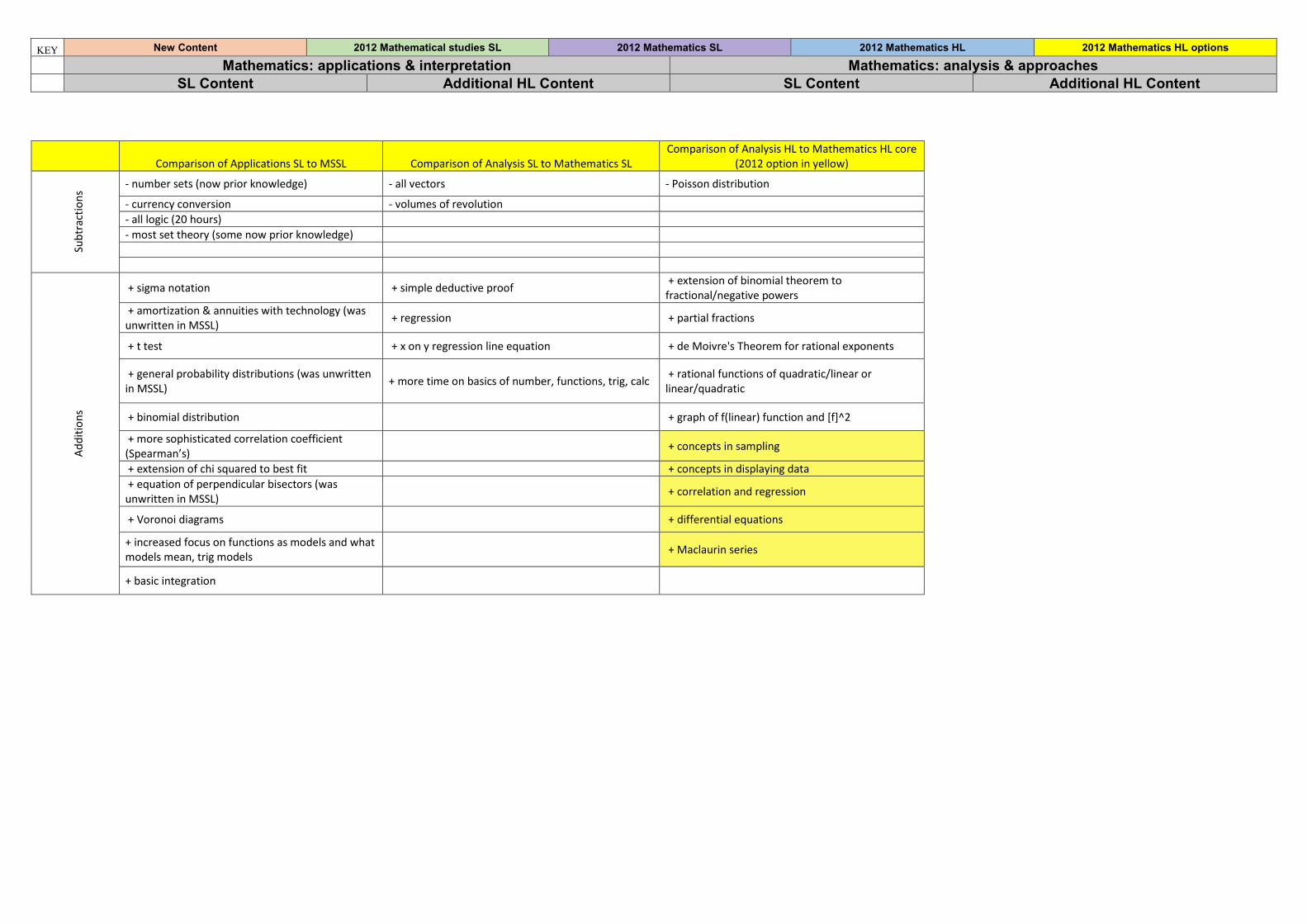
Comparison of Applications SL to MSSL Comparison of Analysis SL to Mathematics SL Comparison of Analysis HL to Mathematics HL core

(2012 option in yellow)

Subt

ract

ions

- number sets (now prior knowledge) - all vectors - Poisson distribution

- currency conversion - volumes of revolution - all logic (20 hours) - most set theory (some now prior knowledge)

Addi

tions

+ sigma notation + simple deductive proof + extension of binomial theorem to fractional/negative powers

+ amortization & annuities with technology (was unwritten in MSSL) + regression + partial fractions

+ t test + x on y regression line equation + de Moivre's Theorem for rational exponents

+ general probability distributions (was unwritten in MSSL) + more time on basics of number, functions, trig, calc + rational functions of quadratic/linear or

linear/quadratic

+ binomial distribution + graph of f(linear) function and [f]^2

+ more sophisticated correlation coefficient (Spearman’s) + concepts in sampling

+ extension of chi squared to best fit + concepts in displaying data + equation of perpendicular bisectors (was unwritten in MSSL) + correlation and regression

+ Voronoi diagrams + differential equations

+ increased focus on functions as models and what models mean, trig models

+ Maclaurin series

+ basic integration

new content 2012 mathematical studies sl 2012 mathematics

Documents