new bounds for the descartes method - max planck society · new bounds for the descartes method ......
TRANSCRIPT
Journal of Symbolic Computation 41 (2006) 49–66www.elsevier.com/locate/jsc
New bounds for the Descartes method
WernerKrandicka,∗, Kurt Mehlhornb
aDepartment of Computer Science, Drexel University, 3141 Chestnut Street, Philadelphia, PA 19104, USAb Max-Planck-Institut für Informatik, Stuhlsatzenhausweg 85, 66123 Saarbrücken, Germany
Received 29 September 2004; accepted 8 February 2005Available online 14 November 2005
Abstract
We give a new bound for the number of recursive subdivisions in the Descartes method for polynomialreal root isolation. Our proof uses Ostrowski’s theory of normal power series from 1950 which has so farbeen overlooked in the literature. We combine Ostrowski’s results with a theorem of Davenport from 1985to obtain our bound. We also characterize normality of cubic polynomials by explicit conditions on theirroots and derive a generalization of one of Ostrowski’s theorems.c© 2005 Elsevier Ltd. All rights reserved.
Keywords: Polynomial real root isolation; Descartes rule of signs; Modified Uspensky method; Recursion tree analysis;Normal polynomials; Root separation bounds; History of mathematics; Möbius transformations; Coefficient signvariations; Cylindrical algebraic decomposition
1. Introduction
Polynomial real root isolation is the task of computing disjoint intervals, each containing asingle root, for all the real roots of a given univariate polynomial with real coefficients.Vincent(1836) showed that polynomial real root isolation can be performed using a test based on theDescartes Rule of Signs. The test evaluates a condition that implies that a given interval containsa single root, and another condition that implies that the interval does not contain any roots. Ifneither condition is satisfied, the interval is bisected and each subinterval is tested recursively. Itis not obvious that Vincent’s method terminates.
Collins and Akritas(1976) proposed a method with a much better worst-case computing timethan Vincent’s method. We will refer to the improved method as “Descartes method”. A study
∗ Corresponding author. Tel.: +1 215 895 2939; fax: +1 215 895 0545.E-mail address:[email protected] (W. Krandick).
0747-7171/$ - see front matterc© 2005 Elsevier Ltd. All rights reserved.doi:10.1016/j.jsc.2005.02.004
50 W.Krandick, K. Mehlhorn / Journal of Symbolic Computation 41 (2006) 49–66
by Johnson(1998) shows thatthe Descartes method typicallyoutperforms Sturm’s methodand other methods for real root isolation. Johnson’s findings are confirmed in experimentsby Rouillier and Zimmermann(2001, Figures 2,3). Recent versions of the Descartes methoduse floating point arithmetic (Johnson and Krandick, 1997; Collins et al., 2002; Rouillier andZimmermann, 2004), parallel computation (Decker and Krandick, 1999, 2001), or they minimizespace requirements (Rouillier and Zimmermann, 2004). Lane and Riesenfeld(1981) describe avariation of the method that uses Bernstein bases.
We give a new bound (Theorem 28) for the number of recursive subdivisions in the Descartesmethod. The bound also applies when Bernstein bases are used. Our proof uses Ostrowski’stheory (Ostrowski, 1950) of normal power series which has so far been overlooked in theliterature. We combine Ostrowski’s results with a theorem ofDavenport (1985) to obtain ourbound. We also characterize normality of cubic polynomials by explicit conditions on their rootsand derive a generalization (Theorem 34) of one of Ostrowski’s theorems.
The history of termination proofs starts withVincent (1836). Alesina and Galuzzi(1998)present Vincent’s original proof in modern mathematical language and provide extensivehistorical information on related earlier andlater results. It seems that Vincent’s methodwas forgotten until Uspensky (1948) modified Vincent’s proof and bounded the number ofrecursive steps required by the method.Ostrowski (1950) used a result from his earlierwork (Ostrowski, 1939) to improve Uspensky’s bound. Ostrowski’s contribution, thoughsummarized inMathematical Reviews(Marden, 1951), was completely overlooked in laterliterature until it became accessible through an electronic database (Alesina and Galuzzi,1999). When Collins and Akritas(1976) improved Vincent’s algorithm they based theiranalysis, later elaborated byCollins and Loos(1982), on Uspensky’s work.Collins andJohnson(1989) improved the analysis significantly, but also their result is strictly weakerthan Ostrowski’s. Eventually, one of Ostrowski’s theorems, the presentTheorem 17, wasindependently rediscovered byAlesina and Galuzzi(1998, Corollary 8.2). The authors gave aconcise and direct proof, but their approach cannot be used to prove the strongerTheorem 34ofthis paper.
In Section 2we review the Descartes method. InSection 3we present Ostrowski’s theoryof normal power series and strengthen one ofhis results that links normality of polynomialsand termination of the Descartes method (Theorem 11). We also present Ostrowski’s sufficientcondition on the roots of a polynomial to guarantee normality (Theorem 16). We use theseresults in Section 4to proveTheorem 23on the proximity of complex roots to those intervalson which the Descartes method recurs. InSection 5we combineTheorem 23with Davenport’sroot separation theorem to obtain new bounds for the recursion tree of the Descartes method. InSection 6we useTheorem 11to characterize the normal cubicpolynomials by explicit conditionson their roots. We gauge the extent of the improvement by applying the Descartes method to2.3 billion cubic polynomials. We use the new result to proveTheorem 34—thus strengtheningTheorem 17.
2. Review of the Descartes method
Definition 1. Let a = (a0, . . . , an) be a finite sequence of real numbers. Thenumber of signvariations in a, var(a), is thenumber of pairs(i , j ) with 0 ≤ i < j ≤ n andai aj < 0 andai+1 = · · · = aj−1 = 0. Let A be the polynomiala0 + a1x + · · · + anxn. The number ofcoefficient sign variationsin A, var(A), is var(a).
W.Krandick, K. Mehlhorn / Journal of Symbolic Computation 41 (2006) 49–66 51
Theorem 2 (Descartes Rule of Signs). For any non-zero real polynomial the number ofcoefficient sign variations exceeds the number of positive real roots—counting multiplicities—bya non-negative, even integer.
Proof. Let A(x) be a non-zero real polynomial. Ifxk is the highest power ofx that dividesA, thepolynomialA/xk has the same number of coefficient sign variations and positive real roots asA,and its constant term is non-zero. Hence, we may assume that the constant term ofA is non-zero.Let a0 be this constant term, letn be the degree ofA, and letan be the leading coefficient. Letv = var(A), and letp be the number of positive real roots ofA, counting multiplicities.
To show thatv and p have the same parity we use an argument given byConkwright(1941).Let z1, . . . , zn ∈ C be the roots ofA. Then
A(x) = an(x − z1) · · · (x − zn), (1)
and hencea0 = A(0) = (−1)nanz1 . . . zn. Sincethenon-real roots occur in complex conjugatepairs, their product is positive. The product of the positive roots is likewise positive, no root iszero sincea0 is non-zero, and the product of the negative real roots has the sign(−1)n−p. Itfollows that the sign ofa0/an is (−1)p. Hencev and p have the same parity.
Gauss(1828) provesv ≥ p by showing that, for any non-zero real polynomialB(x) and anypositive real numbera,
var(B) < var((x − a) · B). (2)
So, in Eq. (1), every positive root ofA contributes at least one sign variation.To show inequality (2) let B = bmxm + · · · + b0, let a > 0, and letC = (x − a)B =
cm+1xm+1 + · · · + c0. If var(B) > 0 let (i , j ) be an index pair that contributes to var(B). Then0 ≤ i < j ≤ m andbi bj < 0 and either j = i + 1 orbi+1 = 0. If σ : R −→ {−1, 0, 1} denotesthe sign function then
σ(ci+1) = σ(bi − abi+1) = σ(bi ).
So, if (i1, j1), . . . , (i k, jk) are all the index pairs that contribute to var(B), and if 0≤ i1 < j1 ≤· · · ≤ i k < jk ≤ m, then
var(ci1+1, . . . , cik+1, cm+1) = var(bi1, . . . , bik , bm) = var(B).
Now let i be the smallest index for whichbi �= 0. Then 0≤ i ≤ i1 andσ(ci ) = σ(−abi ) =−σ(bi ) = −σ(bi1) = −σ(ci1+1), and so
var(C) ≥ var(ci , ci1+1, . . . , cik+1, cm+1) = 1+ var(B).
If var(B) = 0 then var(C) ≥ var(ci , cm+1) = var(−abi , bm) ≥ 1. �
Theorem 2is named after Descartes although he merely stated that there can be as many positivereal roots as there are coefficient sign variations (Descartes, 1954). Over time it became clearthat there are at least as many sign variations as there are positive roots; according toBartolozziand Franci(1993), the assertion was first stated and proved byGauss(1828). Some modernauthors (Albert, 1943; Wang, 2004) seem to be unaware of Gauss’s contribution.
Theorem 3. Let A be a non-zero real polynomial. Ifvar(A) = 0 then Adoes not have anypositive real root; if var(A) = 1 then A has exactly one positive real root.
52 W.Krandick, K. Mehlhorn / Journal of Symbolic Computation 41 (2006) 49–66
Definition 4. Let S be a subring ofR with 1 ∈ S. We define three polynomial transformationsS[x] −→ S[x]. Let A = anxn + · · · + a1x + a0 be an element ofS[x].(1) Thehomothetic transformationof A is the polynomial
H (A) = anxn + 2an−1xn−1+ · · · + 2n−1a1x + 2na0.
(2) TheTaylorshift by1 of A is thepolynomial
T(A) = bnxn + · · · + b1x + b0
wherebk =∑nj=k
( jk
)aj for k ∈ {0, . . . , n}.
(3) Thereciprocal transformationof A is the polynomial
R(A) = a0xn + · · · + an−1x + an.
Note thatR(A) = 0 if andonly if A = 0, and thatx | A implies R(A) = R(A/x).
The Descartes method can now be stated asAlgorithm 1.
Algorithm 1 (Descartes Method). This version is specialized toroot counting inI = (0, 1). Thealgorithm can easily be modified to perform real root isolation.
int roots in I (A ∈ S[x], A �= 0, A squarefree,S⊂ R subring, 1∈ S)d← var(T R(A));if d ≤ 1 return d;B← H (A); C← T(B);if x |C m← 1; else m← 0; Note:m= 1⇐⇒ A(1/2) = 0.return roots in I (B) +m+ roots in I (C);
To show thatAlgorithm 1 is partially correct we relate the roots of transformed realpolynomials to the roots of the untransformed polynomials. Since we want to use bijectivemappings we add the point∞ to C.
Definition 5. Let C = C ∪ {∞} be the Riemann sphere. We define three functionsC −→ C.
h(z)={
z/2, if z ∈ C ;∞, if z= ∞.
t (z) ={
z+ 1, if z ∈ C ;∞, if z= ∞.
r (z) =
1/z, if z ∈ C− {0} ;∞, if z= 0 ;0, if z=∞.
The functionsh, t , andr are elements of the group ofMöbius transformations. These are allfunctionsC −→ C given by
z �−→ az+ b
cz+ d(3)
with a, b, c, d ∈ C andad− bc �= 0.Anderson(1999) explains how formula (3) handles divisionby 0 and evaluation at∞. Also Carathéodory(1964) andHenrici (1974) discussthe propertiesof Möbius transformations.
W.Krandick, K. Mehlhorn / Journal of Symbolic Computation 41 (2006) 49–66 53
Remark 6. Let A ∈ R[x], and letn = deg(A); we adopt the convention that deg(0) = 0 andldcf(0) = 0. Then, for allz ∈ C,
H (A)(z) = 2n A(h(z)),
T(A)(z) = A(t (z)),
R(A)(z) ={
zn A(r (z)), if z �= 0;ldcf(A), if z= 0.
So, for allz ∈ C,
T H(A)(z) = 2n A((h ◦ t)(z)),
T R(A)(z) ={(t (z))n A((r ◦ t)(z)), if z �= −1;ldcf(A), if z= −1.
Remark 7. By Remark 6, the following statements hold for all polynomialsA ∈ R[x].1. The functionh maps the roots ofH (A) one-to-one onto the roots ofA; in particular, the roots
of H (A) in (0, 1) correspond to the roots ofA in (0, 1/2).2. The functiont maps the roots ofT(A) one-to-one onto the roots ofA.3. The functionr maps the non-zero roots ofR(A) one-to-one onto the non-zero roots ofA; the
roots ofR(A) are non-zero unlessA = 0.4. The functionh ◦ t maps the roots ofT H(A) one-to-one onto the roots ofA; in particular, the
roots ofT H(A) in (0, 1) correspond to the roots ofA in (1/2, 1).5. The functionr ◦ t maps those roots ofT R(A) that are different from−1 one-to-one onto the
non-zero roots ofA; the roots ofT R(A) are different from−1 unlessA = 0. The positivereal roots ofT R(A) correspond to the roots ofA in (0, 1).
Theorem 8. Algorithm1 is partially correct.
Proof. Combine the observations (1), (4), and (5) of Remark 7with Theorem 3. �
3. Ostrowski’s theory
Definition 9. A powerseries
+∞∑k=−∞
akzk
with non-negative real coefficients isnormal(Ostrowski, 1939) if
(1) a2k ≥ ak−1ak+1 for all indicesk, and
(2) ah > 0 andaj > 0 for indicesh < j impliesah+1, . . . , aj−1 > 0.
In 1950, Ostrowski linked the normality of a polynomial and the Descartes rule. He statedhis result (Ostrowski, 1950, Lemma 1) for polynomials all of whose coefficients are positive.Generalizing slightly we show inTheorem 11that it suffices to require that the leading coefficientbe positive.
Definition 10. A polynomial with real coefficients ispositive if its leading coefficient is positive.
Theorem 11. A positive polynomial A(x) is normal if and only ifvar((x − α)A(x)) = 1 for allpositive real numbersα.
Proof. (i) Let A(x) be positive and normal, and letα be a positive real number. There is a non-negativeintegerm suchthat A(x) = B(x) · xm whereB(x) is normal and all the coefficients of
54 W.Krandick, K. Mehlhorn / Journal of Symbolic Computation 41 (2006) 49–66
B(x) are positive. LetB(x) = bnxn + · · · + b1x + b0. Then
bn−1
bn≥ bn−2
bn−1≥ · · · ≥ b0
b1
and hence
bn−1
bn− α ≥ bn−2
bn−1− α ≥ · · · ≥ b0
b1− α.
Since alsobn > 0 and−αb0 < 0, the polynomial
(x − α)B(x) = bnxn+1+ bn
(bn−1
bn− α
)xn + · · · + b1
(b0
b1− α
)x − αb0
has exactly 1 coefficient sign variation. And so,
1= var((x − α)B(x)) = var((x − α)B(x) · xm) = var((x − α)A(x)).
(ii) Conversely, letA(x) be positive but not normal. There is a non-negative integerm suchthat A = B(x) · xm whereB(x) has a non-zero constant term. Moreover, the polynomialB(x)
is positive and not normal—and hence non-constant. For any real numberα let C(α)(x) =(x− α)B(x). Then var((x− α)A(x)) = var(C(α)(x)), and it suffices to find a positive numberα
such that var(C(α)(x)) �= 1.Let B(x) = bnxn + · · · + b1x + b0. Then n ≥ 1 and bn > 0 and b0 �= 0. Let
C(α)(x) = c(α)n+1xn+1+· · ·+c(α)
1 x+c(α)0 . Thenc(α)
0 = −αb0, c(α)k = bk−1− αbk for 1≤ k ≤ n,
andc(α)n+1 = bn.
If var(B(x)) ≥ 2 chooseα so small that, for allk with 1 ≤ k ≤ n, the signs ofc(α)k andbk−1
are equal wheneverbk−1 �= 0; then var(C(α)(x)) ≥ var(B(x)) ≥ 2.If var(B(x)) = 1 the polynomialB(x) has exactly one positive real root by the Descartes
rule. So, for anyα > 0, the polynomialC(α)(x) has two positive real roots, and, again by theDescartes rule, var(C(α)(x)) ≥ 2.
Finally, assume var(B(x)) = 0. Then, sincebn > 0, all the coefficients ofB(x) are non-negative. If all the coefficients ofB(x) are positive, then, sinceB(x) is not normal, there isan indexk with 1 ≤ k ≤ n − 1 such that 0< bk/bk+1 < bk−1/bk. Chooseα suchthatbk/bk+1 < α < bk−1/bk. Now α > 0 andc(α)
n+1 = bn > 0, c(α)k+1 = bk − αbk+1 < 0 and
c(α)k = bk−1 − αbk > 0, and hence var(C(α)(x)) ≥ 2. If not all the coefficients ofB(x) are
positive, there is a zero-coefficient. Letbk be the zero-coefficient with the highest index; thenc(α)
k+1 < 0 for anypositiveα. Sinceb0 > 0 there isan index j < k suchthat bj+1 = 0 and
bj > 0; thenc(α)j+1 > 0. Nowc(α)
0 < 0 implies var(C(α)(x)) ≥ 2 also in this case. �
By Theorem 11, the Descartes rule will reveal the existence of a single positive root of a positivepolynomial if the other rootsα1, . . . , αn−1 are such that(x − α1) · · · (x − αn−1) is a normalpolynomial.
Theorem 12. A positive linear polynomial is normal if and only if its root is negative or zero.
Proof. Let A be a positive linear polynomial, and letα ∈ R be its root. Then there is a positivereal numbera suchthat A(x) = a(x− α) = ax− aα. Now A is normal if and only if−aα ≥ 0,that is, if and only if α ≤ 0. �
W.Krandick, K. Mehlhorn / Journal of Symbolic Computation 41 (2006) 49–66 55
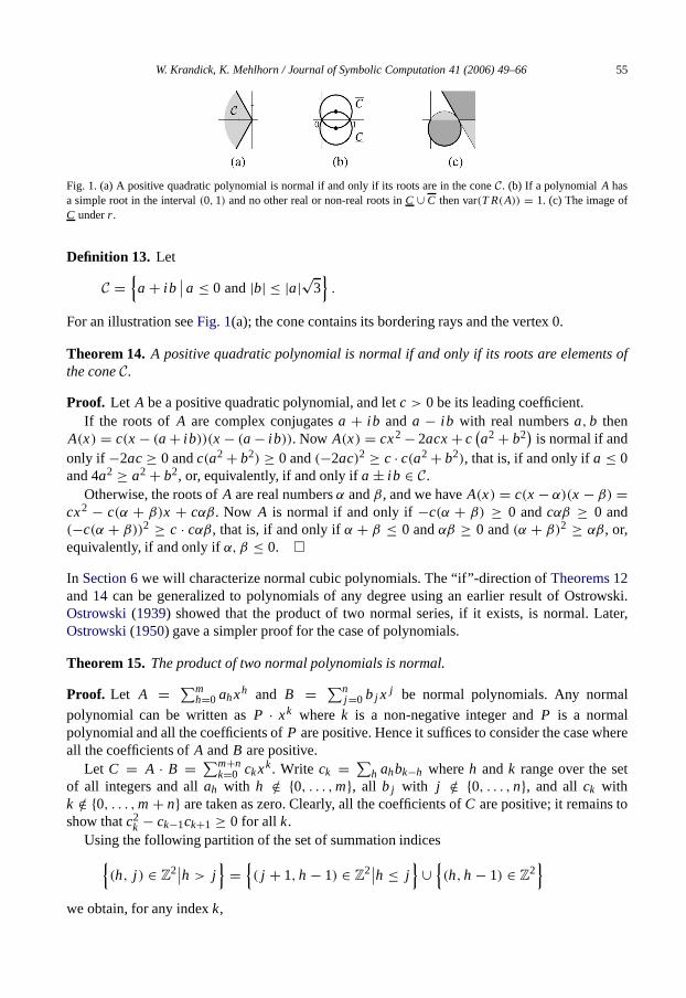
Fig. 1. (a) A positive quadratic polynomial isnormal if and only if its roots are in the coneC. (b) If a polynomialA hasa simple root in the interval(0, 1) and no other real or non-real roots inC ∪ C then var(T R(A)) = 1. (c) The image ofC underr .
Definition 13. Let
C ={a+ ib
∣∣ a ≤ 0 and|b| ≤ |a|√3}
.
For an illustration seeFig. 1(a); the cone contains its bordering rays and the vertex 0.
Theorem 14. A positive quadratic polynomial is normal if and only if its roots are elements ofthe coneC.
Proof. Let A be a positive quadratic polynomial, and letc > 0 beits leading coefficient.If the roots of A are complex conjugatesa + ib and a − ib with real numbersa, b then
A(x) = c(x− (a+ ib))(x− (a− ib)). Now A(x) = cx2− 2acx+ c(a2+ b2
)is normal if and
only if −2ac≥ 0 andc(a2+ b2) ≥ 0 and(−2ac)2 ≥ c · c(a2+ b2), that is, ifand only ifa ≤ 0and 4a2 ≥ a2+ b2, or, equivalently, if and only ifa± ib ∈ C.
Otherwise,the roots ofA are real numbersα andβ, and wehaveA(x) = c(x− α)(x − β) =cx2 − c(α + β)x + cαβ. Now A is normal if and only if−c(α + β) ≥ 0 andcαβ ≥ 0 and(−c(α + β))2 ≥ c · cαβ, that is, ifand only ifα + β ≤ 0 andαβ ≥ 0 and(α + β)2 ≥ αβ, or,equivalently, if and only ifα, β ≤ 0. �
In Section 6we will characterize normal cubic polynomials. The “if”-direction ofTheorems 12and14 can be generalized to polynomials of any degree using an earlier result of Ostrowski.Ostrowski(1939) showed that the product of two normal series, if it exists, is normal. Later,Ostrowski(1950) gave asimpler proof for the case of polynomials.
Theorem 15. The product of two normal polynomials is normal.
Proof. Let A = ∑mh=0 ahxh and B = ∑n
j=0 bj x j be normal polynomials. Any normal
polynomial can be written asP · xk wherek is a non-negative integer andP is a normalpolynomial and all the coefficients ofP are positive. Hence it suffices to consider the case whereall the coefficients ofA andB are positive.
Let C = A · B = ∑m+nk=0 ckxk. Write ck = ∑
h ahbk−h whereh andk range over the setof all integers and allah with h /∈ {0, . . . , m}, all bj with j /∈ {0, . . . , n}, and all ck withk /∈ {0, . . . , m+ n} are taken as zero. Clearly, all the coefficients ofC are positive; it remains toshow thatc2
k − ck−1ck+1 ≥ 0 for all k.Using the following partition of the set of summation indices
{(h, j ) ∈ Z
2∣∣h > j
}=
{( j + 1, h− 1) ∈ Z
2∣∣h ≤ j
}∪
{(h, h− 1) ∈ Z
2}
we obtain, for any indexk,

56 W.Krandick, K. Mehlhorn / Journal of Symbolic Computation 41 (2006) 49–66
c2k − ck−1ck+1
=∑h≤ j
ahaj bk−hbk− j +∑h> j
ahaj bk−hbk− j
−∑h≤ j
ahaj bk−h+1bk− j−1−∑h> j
ahaj bk−h+1bk− j−1
=∑h≤ j
ahaj bk−hbk− j +∑h≤ j
aj+1ah−1bk− j−1bk−h+1 +∑
h
ahah−1bk−hbk−h+1
−∑h≤ j
ahaj bk−h+1bk− j−1−∑h≤ j
aj+1ah−1bk− j bk−h −∑
h
ahah−1bk−h+1bk−h
=∑h≤ j
(ahaj − ah−1aj+1)(bk− j bk−h − bk− j−1bk−h+1),
that is,
c2k − ck−1ck+1 =
∑h≤ j
(ahaj − ah−1aj+1)(bk− j bk−h − bk− j−1bk−h+1). (4)
SinceA is normal anda0, . . . , am are positive, one has
am−1
am≥ am−2
am−1≥ · · · ≥ a0
a1,
and henceahaj − ah−1aj+1 ≥ 0 for all h ≤ j ; the analogous statement holds for thecoefficients ofB. Hence each summand on the right-hand side of Eq. (4) is non-negative, andthusc2
k − ck−1ck+1 ≥ 0 for all k. �
Theorem 16. If the roots of a positive polynomial are in the coneC then the polynomial isnormal.
Proof. Let A be a positive polynomial all of whose roots are elements of the coneC. Thecomplete factorization ofA over the field of real numbers is a product of linear and quadraticfactors. We may assume that all these factors are positive. Since all the roots are in the coneC,Theorems 12and14 apply, and each factor is normal. Thus, byTheorem 15, the polynomialAis normal. �
Of all the theorems in this section, we will invoke onlyTheorem 17in Sections 4and5.
Theorem 17. If the roots of a non-zero polynomial A(x) are in the coneC then var((x −α)A(x)) = 1 for all positive real numbersα.
Proof. Let A be a non-zero polynomial and such that all of its roots are elements of theconeC. If A is positive thenA is normal by Theorem 16, and henceTheorem 11impliesvar((x − α)A(x)) = 1 for all positive α. If A is not positive then−A is positive and theroots of−A are elements of the coneC. Hence, as before, var((x − α)(−A)(x)) = 1, butvar((x − α)(−A)(x)) = var((x − α)A(x)). �
4. Three circles
By Theorem 17, Algorithm 1will stop calling itself when it encounters a polynomialT R(A)
that has exactlyone positive root and whose other roots are elements of the coneC. We want tostate this condition in terms of the roots of the polynomialA. SinceA is non-zero,Remark 7(5)
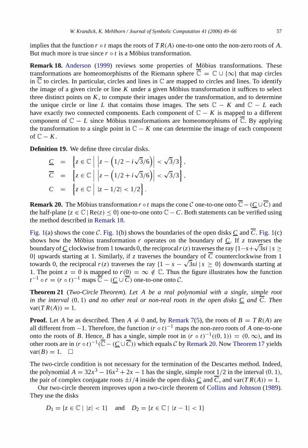
W.Krandick, K. Mehlhorn / Journal of Symbolic Computation 41 (2006) 49–66 57
implies that the functionr ◦ t maps the roots ofT R(A) one-to-one onto the non-zero roots ofA.But much more is true sincer ◦ t is a Möbius transformation.
Remark 18. Anderson(1999) reviews someproperties of Möbius transformations. Thesetransformations are homeomorphisms of the Riemann sphereC = C ∪ {∞} that map circlesin C to circles. In particular, circles and lines inC are mapped to circles and lines. To identifythe image of a given circle or lineK under a given Möbius transformation it suffices to selectthree distinct points onK , to compute their images under the transformation, and to determinethe unique circle or lineL that containsthose images. The setsC − K and C − L eachhave exactly two connected components. Each component ofC − K is mapped to a differentcomponent ofC − L since Möbius transformations are homeomorphisms ofC. By applyingthe transformation to a single point inC − K one can determine the image of each componentof C− K .
Definition 19. We define three circular disks.
C ={z ∈ C
∣∣∣ ∣∣∣z− (1/2− i
√3/6
)∣∣∣ <√
3/3}
,
C ={z ∈ C
∣∣∣∣∣∣z− (
1/2+ i√
3/6)∣∣∣ <√
3/3}
,
C ={z ∈ C
∣∣∣ |z− 1/2| < 1/2}
.
Remark 20. The Möbius transformationr ◦ t maps the coneC one-to-one ontoC− (C∪C) andthe half-plane{z ∈ C |Re(z) ≤ 0} one-to-one ontoC−C. Both statementscan be verified usingthe method described inRemark 18.
Fig. 1(a) shows the coneC. Fig. 1(b) shows the boundaries of the open disksC andC. Fig. 1(c)shows how the Möbius transformationr operates on the boundary ofC. If z traverses theboundary ofC clockwise from 1 towards 0, the reciprocalr (z) traverses the ray{1−s+√3si | s≥0} upwards starting at 1. Similarly, if z traverses the boundary ofC counterclockwise from 1towards 0, the reciprocalr (z) traverses the ray{1− s − √3si | s ≥ 0} downwards starting at1. The pointz = 0 is mapped tor (0) = ∞ /∈ C. Thusthe figure illustrates how the functiont−1 ◦ r = (r ◦ t)−1 mapsC− (C ∪ C) one-to-one ontoC.
Theorem 21 (Two-CircleTheorem). Let A be a realpolynomial with a single, simple rootin the interval (0, 1) and no other real or non-real roots in the open disks Cand C. Thenvar(T R(A)) = 1.
Proof. Let A be as described. ThenA �= 0 and, byRemark 7(5), the roots ofB = T R(A) areall different from−1. Therefore, the function(r ◦ t)−1 maps the non-zero roots ofA one-to-oneonto the roots ofB. Hence, B has a single, simple root in(r ◦ t)−1((0, 1)) = (0,∞), anditsother roots are in(r ◦ t)−1(C− (C∪C)) which equalsC by Remark 20. Now Theorem 17yieldsvar(B) = 1. �
The two-circle condition is not necessary for thetermination of the Descartes method. Indeed,thepolynomialA = 32x3− 16x2+ 2x − 1 has the single, simple root 1/2 in the interval(0, 1),the pair of complex conjugate roots±i /4 inside theopen disksC andC, and var(T R(A)) = 1.
Our two-circle theorem improves upon a two-circle theorem ofCollins andJohnson(1989).They use the disks
D1 = {z ∈ C | |z| < 1} and D2 = {z ∈ C | |z− 1| < 1}
58 W.Krandick, K. Mehlhorn / Journal of Symbolic Computation 41 (2006) 49–66
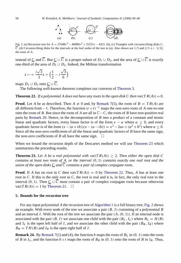
Fig. 2. (a) Recursion tree forA = 27648x3−46080x2+25251x−4321. (b), (c) Triangles withcircumscribing disksC,C. (d) Circumscribing disks for the intervals atthe leaf nodes of the tree in (a). Also shown are 1/3 and 2/3± i · 5/32,the roots ofA.
instead ofC andC. But C ∪ C is a proper subset ofD1 ∪ D2, and the area ofC ∪ C is exactlyone-third of the area ofD1 ∪ D2. Indeed, the Möbius transformation
z �−→ i√
3
3z+
(1
2− i
√3
6
)
mapsD1 ∪ D2 ontoC ∪ C.The following well-known theorem completes our converse ofTheorem 3.
Theorem 22. If a polynomial A does not have any roots in the open disk C thenvar(T R(A))=0.
Proof. Let A be as described. ThenA �= 0 and, byRemark 7(5), the roots ofB = T R(A) areall different from−1. Therefore, the function(r ◦ t)−1 maps the non-zero roots ofA one-to-oneonto the roots ofB. But since the roots ofA are all inC−C, the roots ofB have non-positive realparts byRemark 20. Hence, in the decomposition ofB into a product of a constant and moniclinear and quadratic factors, every linear factor is of the formx − α whereα ≤ 0, and everyquadratic factor is of the form(x− (a+ ib))(x− (a− ib)) = x2−2ax+ (a2+b2) wherea ≤ 0.Since all the non-zero coefficients of all the linear and quadratic factors ofB have the same sign,thenon-zero coefficients ofB all have the same sign.�
When we bound the recursion depth of the Descartes method we will useTheorem 23whichsummarizes the preceding results.
Theorem 23. Let A be a realpolynomial withvar(T R(A)) ≥ 2. Then either the open disk Ccontains at least two roots of A, or the interval(0, 1) contains exactly one real root and theunion of the open disks CandC contains a pair of complex conjugate roots.
Proof. If A has no root inC then var(T R(A)) = 0 by Theorem 22. Thus, A has at least oneroot in C. If this is the only root inC, the root is real and it is, in fact, the only real root in theinterval (0, 1). ThenC ∪ C must contain a pair of complex conjugate roots because otherwisevar(T R(A)) = 1 byTheorem 21. �
5. Bounds for the recursion tree
For any input polynomialA the recursion tree ofAlgorithm 1is a full binary tree;Fig. 2showsan example. With every node of the tree we associate a pair(B, I ) consisting of a polynomialBand an intervalI . With the root of the tree we associate the pair(A, (0, 1)). If an internal node isassociated with the pair(B, I ) we associate one child with the pair(BL, I L) whereBL = H (B)
and I L is the open left half ofI , and we associate the other child with the pair(BR, IR) whereBR = T H(B) andIR is the open right half of I .
Remark 24. By Remark 7(1) and (4), the functionh maps the roots ofBL in (0, 1) onto the rootsof B in I L , and the functionh ◦ t maps the roots ofBR in (0, 1) onto the roots ofB in IR. Thus,

W.Krandick, K. Mehlhorn / Journal of Symbolic Computation 41 (2006) 49–66 59
there is a sequence of elements of{h, t} whose compositionm maps the roots ofB in (0, 1) ontothe roots of the input polynomialA in I . Whenm maps the interval(0, 1) onto the intervalI ittransforms at the same time the disksC, C andC of Section 4. Thesedisks are the circumscribingdisks of isosceles triangles with base(0, 1) and base angles 45◦, −60◦ and 60◦, respectively, asshown inFig. 2. But h, t and, hence,m are Möbius transformations and thus preserve angles(Anderson, 1999). Moreover, the transformationsh, t and, hence,m map straight lines inC ontostraight lines inC and circles inC onto circles inC. Therefore, the imagesm(C), m(C) andm(C) are the circumscribing disks of the isosceles triangles with baseI and base angles 45◦,−60◦ and 60◦, respectively.Fig. 2 shows the disks that are considered at the leaf nodes of aparticular recursion tree.
The depth of the recursion tree can be bounded using the root separation theorem ofMahler(1964). To obtain a bound that also covers the width of the tree we use a generalization byDavenport(1985) of Mahler’s theorem in a form due toJohnson(1998).
Definition 25. Let A = anxn + · · · + a1x + a0 be a non-zero polynomial of degreen withcomplex coefficients and the complex rootsα1, . . . , αn. The Euclidean normof A is |A|2 =(a2
n + · · · + a20)1/2, themeasure of A is M(A) = |an| ·∏n
i=1 max(1, |αi |), and thediscriminantof A is D(A) = a2n−2
n∏
i< j (αi − α j )2.
Remark 26. A theorem of Landau (1905) implies M(A) ≤ |A|2. The inequality wasindependently rediscovered more than once.Ostrowski(1961) summarizes its history and provesa generalization.Mignotte(1974, 1982) gives a short elementary proof. The discriminantD(A)
is known to be a polynomial in the coefficients ofA (van der Waerden, 1949); henceD(A) ≥ 1if A is a squarefree integer polynomial.
Theorem 27. Let A be a non-zero complex polynomial of degree n with the rootsα1, . . . , αn. Letk be an integer,1≤ k ≤ n, and let(β1, . . . , βk) be a sequence of roots of A such that
βi �∈ {α1, . . . , αi } and |βi | ≤ |αi | for all i ∈ {1, . . . , k}.Then
k∏i=1
|αi − βi | ≥ 3k/2D(A)1/2M(A)−n+1n−k−n/2.
Proof. Johnson(1998). �
Theorem 28. Let A be a non-zero real polynomial of degree n, measure M, and discriminant D.Let the integers h≥ 0 and k≥ 1 be such that k is the number of internal nodes of depth h in therecursion tree ofAlgorithm1 with input A wheredepthis the distance from the root. Then
(1) k ≤ n, and(2) 2(1−h)k > 3k D1/2M−n+1n−k−n/2.
Proof. Let I1 < · · · < Ik be the open subintervals of(0, 1) that are associated with the internalnodes of depthh, and letA1, . . . , Ak be the corresponding polynomials. The intervals have width2−h. For every indexi ∈ {1, . . . , k} let Ci , Ci andCi be the circumscribing disks of the isoscelestriangles with baseIi and base angles 45◦, −60◦ and 60◦, respectively. ByRemark 24the rootsof Ai in the disksC, C andC, correspond, respectively, to the roots ofA in the disksCi , Ci andCi . But the polynomialsAi are at internal nodes of the recursion tree, so var(T R(Ai )) ≥ 2, and
60 W.Krandick, K. Mehlhorn / Journal of Symbolic Computation 41 (2006) 49–66
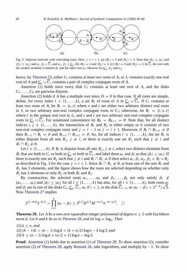
Fig. 3. Adjacent intervals with coinciding roots. Here,j = i + 1. (a) |Ri | = 3 and|Rj | = 2. Note that|βi | ≤ |αi | and|β j | ≤ |α j | andαi , βi ∈ Ci andα j , β j ∈ Ci . (b) |Ri | = 2 and|Rj | = 3. (c) |Ri | = 3 and|Rj | = 3. In Ci the root withthe smaller modulus is labeledβi and the other rootαi ; likewise forC j , β j andα j .
hence, byTheorem 23, either Ci contains at least two roots ofA, or Ii contains exactly one realroot of A andCi ∪ Ci contains a pair of complex conjugate roots ofA.
Assertion (1) holds since every diskCi contains at least one root ofA, and the disksC1, . . . , Ck are pairwise disjoint.
Assertion(2) holds if A has amultiple root sinceD = 0 in thatcase. If all roots are simple,define, for every indexi ∈ {1, . . . , k}, a setRi of roots of A in Ci ∪ Ci . If Ci contains atleast two roots ofA, let Ri = {s, t} wheres and t are either two arbitrary distinct real rootsin Ii or two arbitrary non-real complex conjugate roots inCi ; otherwise, let Ri = {r, s, t}wherer is the unique real root inIi , ands andt are two arbitrary non-real complex conjugateroots in Ci ∪ Ci . For notational convenience letR0 = Rk+1 = ∅. Note that, for all distinctindicesi , j ∈ {1, . . . , k}, the intersection ofRi and Rj is either empty or it consists of twonon-real complex conjugate roots andj = i − 1 or j = i + 1. Moreover, ifRi ∩ Ri+1 �= ∅then Ri−1 ∩ Ri = ∅ and Ri+1 ∩ Ri+2 = ∅. So, for all indices i ∈ {1, . . . , k}, the setRi iseither disjoint from all setsRj , j �= i , or there is exactly one setRj suchthat j �= i andRi ∩ Rj �= ∅.
Let i ∈ {1, . . . , k}. If Ri is disjoint from all setsRj , j �= i , select two distinct elements fromRi that are both inCi or both inCi or both inCi , and label themαi andβi so that|βi | ≤ |αi |. Ifthere is exactly one setRj suchthat j �= i andRi ∩ Rj �= ∅ then selectαi , βi , α j , β j ∈ Ri ∪ Rj
as described inFig. 3 for the casej = i + 1. SinceRi ∩ Rj �= ∅, at least one of the setsRi andRj has 3 elements, and the figure shows how the roots are selected depending on whether onlyRi has 3 elements or onlyRj or bothRi andRj .
By construction, the selected rootsα1, . . . , αk and β1, . . . , βk not only satisfy βi �∈{α1, . . . , αi } and|βi | ≤ |αi | for all i ∈ {1, . . . , k} but also,for all i ∈ {1, . . . , k}, both rootsαi
andβi are in one of the disksCi , Ci , Ci , or, if i > 1, in the diskCi−1, so|αi − βi | < 21−h/√
3.Now Theorem 27implies
2(1−h)k3−k/2 >
k∏i=1
|αi − βi | ≥ 3k/2D1/2M−n+1n−k−n/2. �
Theorem 29. Let A be a non-zero squarefree integer polynomial of degree n≥ 2 with Euclideannorm d. Let h and k be as inTheorem28, and letlog= log2. Then
(1) k ≤ n, and(2) (h− 1)k < (n− 1) logd + (k+ n/2) logn− k log 3, and(3) h ≤ (n− 1) logd + (n/2+ 1) logn− log 3.
Proof. Assertion(1) holds due to assertion(1) of Theorem 28. To show assertion(2), considerassertion(2) of Theorem 28, apply Remark 26, take logarithms, and multiply by−1. To show
W.Krandick, K. Mehlhorn / Journal of Symbolic Computation 41 (2006) 49–66 61
assertion(3), consider assertion(2) and collect all terms involvingk on one side to obtaink(h − 1 − logn + log 3) < (n − 1) logd + n/2 logn. If h − 1 − logn + log 3 < 0 thenassertion(3) clearly holds. If, on the other hand,h − 1− logn+ log 3≥ 0 thenk ≥ 1 impliesh − 1− logn + log 3 < (n − 1) logd + n/2 logn, andhence assertion(3) holds alsoin thiscase. �
Remark 30. Theorem 29is stronger than an earlier result byKrandick (1995, Satz47), and theproof is shorter. The theorem implies the dominance relationshk � n log(nd) andh � n log(nd)
which can be used in an asymptotic computing time analysis ofAlgorithm 1when the ringS ofcoefficients isZ; thenotation� is due toCollins (1974).
6. Normal cubics
By Theorem 16any positive polynomial whose roots are in the coneC is normal. ByTheorems 12and 14 the converse holds for linear and quadratic polynomials. For cubicpolynomials, however, the converse is false. Indeed, the normal polynomialx3+5x2+16x+30has roots−1± 3i /∈ C. Theorems 31and32 together completely characterize the normal cubicpolynomials.
Theorem 31. Let A be a positive polynomial all of whose roots are real. Then A is normal if andonly if the roots are all non-positive.
Proof. If the roots ofA are all non-positive thenTheorem 16implies thatA is normal. Otherwise,A has a positive root. In this case, var((x − 1)A(x)) > 1 byTheorem 2, andA is not normal byTheorem 11. �
Theorem 32. Let A be a positive cubic polynomial whose roots are a and b± ic where a, b, care real numbers. Then A is normal if and only if
a ≤ 0 and (5)
b ≤ 0 and (6)
c2− 3b2− 2ab− a2 ≤ 0 and (7)
c4+ 2b2c2+ 2abc2− a2c2+ b4+ 2ab3+ 3a2b2 ≥ 0. (8)
Proof. We may assume thatA is monic sinceA is normal if and only ifA/ldcf(A) is normal.Hence,
A = (x − a) · (x − (b+ ic)) · (x − (b− ic))
and thus
A = x3+ a2x2+ a1x + a0
where
a2 = −a− 2b,
a1 = 2ab+ b2+ c2,
a0 = −ab2− ac2.
62 W.Krandick, K. Mehlhorn / Journal of Symbolic Computation 41 (2006) 49–66
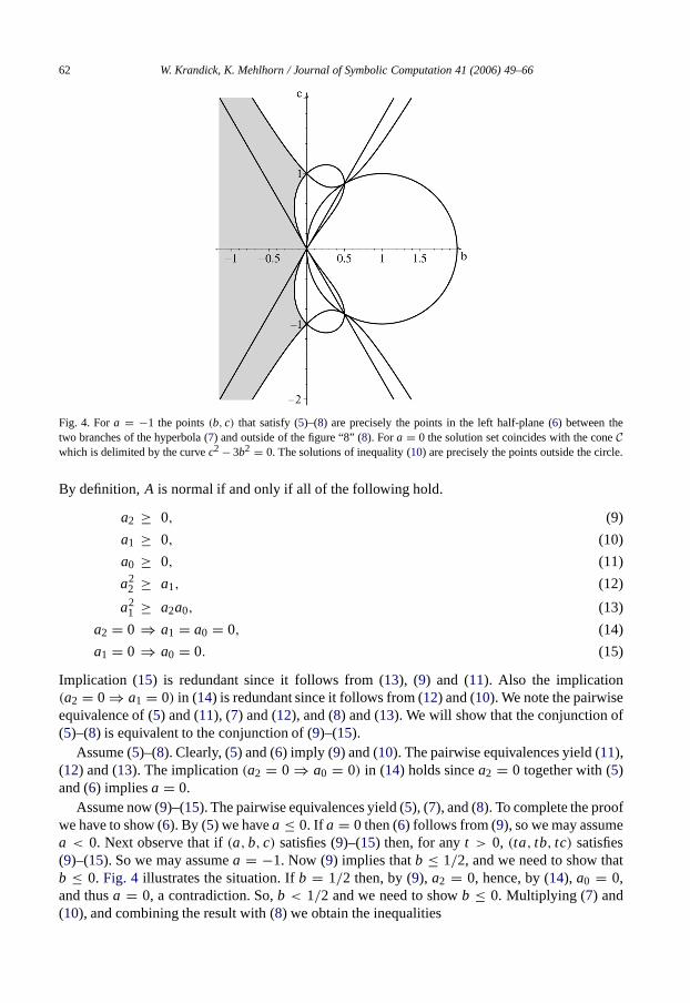
Fig. 4. Fora = −1 thepoints (b, c) that satisfy (5)–(8) are precisely the points in the left half-plane (6) between thetwo branches of the hyperbola (7) andoutside of the figure “8” (8). Fora = 0 the solution set coincides with the coneCwhich is delimited by the curvec2− 3b2 = 0. The solutions of inequality (10) are precisely the points outside the circle.
By definition, A is normal if and only if all of the following hold.
a2 ≥ 0, (9)
a1 ≥ 0, (10)
a0 ≥ 0, (11)
a22 ≥ a1, (12)
a21 ≥ a2a0, (13)
a2 = 0 ⇒ a1 = a0 = 0, (14)
a1 = 0 ⇒ a0 = 0. (15)
Implication (15) is redundant since it follows from (13), (9) and (11). Also the implication(a2 = 0⇒ a1 = 0) in (14) is redundant since it follows from (12) and (10). We note the pairwiseequivalence of (5) and (11), (7) and (12), and (8) and (13). We will show that the conjunction of(5)–(8) is equivalent to the conjunction of (9)–(15).
Assume (5)–(8). Clearly, (5) and (6) imply (9) and (10). The pairwise equivalences yield (11),(12) and (13). The implication (a2 = 0⇒ a0 = 0) in (14) holds sincea2 = 0 togetherwith (5)and (6) impliesa = 0.
Assume now (9)–(15). The pairwise equivalences yield (5), (7), and (8). To complete the proofwe have to show (6). By (5) we havea ≤ 0. If a = 0 then (6) follows from (9), so we may assumea < 0. Next observe that if(a, b, c) satisfies (9)–(15) then, for anyt > 0, (ta, tb, tc) satisfies(9)–(15). So we may assumea = −1. Now (9) implies thatb ≤ 1/2, and we need to show thatb ≤ 0. Fig. 4 illustrates the situation. Ifb = 1/2 then, by (9), a2 = 0, hence, by (14), a0 = 0,and thusa = 0, a contradiction. So,b < 1/2 and weneed to showb ≤ 0. Multiplying (7) and(10), and combining the result with (8) we obtain the inequalities
W.Krandick, K. Mehlhorn / Journal of Symbolic Computation 41 (2006) 49–66 63
(c2− 3b2+ 2b− 1)(−2b+ b2+ c2) ≤ 0
≤ c4+ 2b2c2+ 2abc2− a2c2+ b4+ 2ab3+ 3a2b2.
Collecting all the terms on the left-hand side and factoring yields
−2b(2b− 1)((b− 1)2+ c2) ≤ 0,
so 0< b < 1/2 is impossible,and we haveb ≤ 0 as desired. �
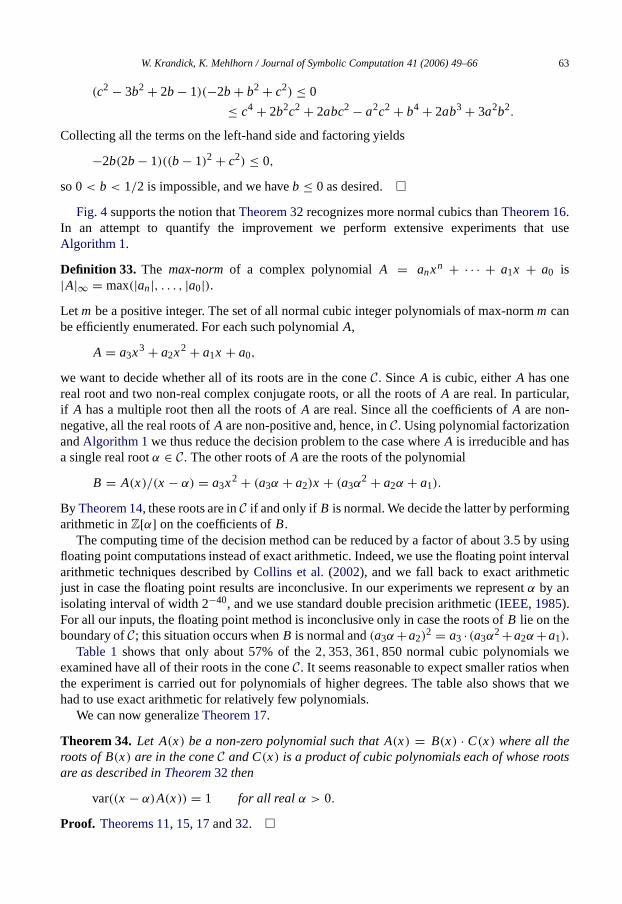
Fig. 4supports the notion thatTheorem 32recognizes more normal cubics thanTheorem 16.In an attempt to quantify the improvement we perform extensive experiments that useAlgorithm 1.
Definition 33. The max-norm of a complex polynomialA = anxn + · · · + a1x + a0 is|A|∞ = max(|an|, . . . , |a0|).Let m be a positive integer. The set of all normal cubic integer polynomials of max-normm canbe efficiently enumerated. For each such polynomialA,
A = a3x3+ a2x2+ a1x + a0,
we want todecide whether all of its roots are in the coneC. SinceA is cubic, eitherA has onereal root and two non-real complex conjugate roots, or all the roots ofA are real. In particular,if A has amultiple root then all the roots ofA are real. Since all the coefficients ofA are non-negative, all the real roots ofA are non-positive and, hence, inC. Using polynomial factorizationandAlgorithm 1we thus reduce the decision problem to the case whereA is irreducible and hasa single real rootα ∈ C. Theother roots ofA are the roots of the polynomial
B = A(x)/(x − α) = a3x2+ (a3α + a2)x + (a3α2 + a2α + a1).
By Theorem 14, these roots are inC if andonly if B is normal. We decide the latter by performingarithmetic inZ[α] on the coefficients ofB.
The computing time of the decision method can be reduced by a factor of about 3.5 by usingfloating point computations instead of exact arithmetic. Indeed, we use the floating point intervalarithmetic techniques described byCollins et al.(2002), and we fall back to exact arithmeticjust in case the floating point results are inconclusive. In our experiments we representα by anisolating interval of width 2−40, and we use standard double precision arithmetic (IEEE, 1985).For all our inputs, the floating point method is inconclusive only in case the roots ofB lie on theboundary ofC; this situation occurs whenB is normal and(a3α+a2)
2 = a3 · (a3α2+a2α+a1).
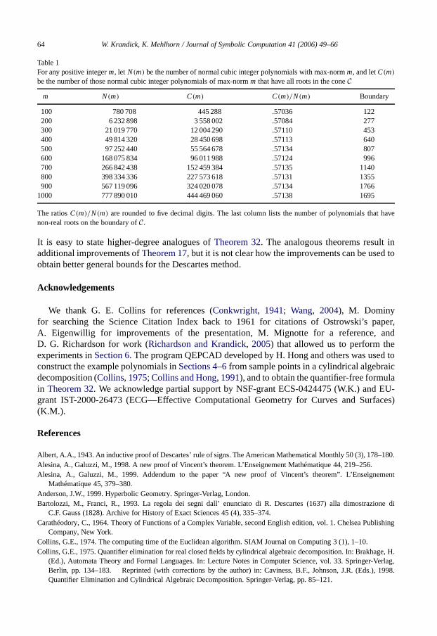
Table 1shows that only about 57% of the 2, 353, 361, 850 normal cubic polynomials weexamined have all of their roots in the coneC. It seems reasonable to expect smaller ratios whenthe experiment is carried out for polynomials of higher degrees. The table also shows that wehad to use exact arithmetic for relatively few polynomials.
We can now generalizeTheorem 17.
Theorem 34. Let A(x) be a non-zero polynomial such that A(x) = B(x) · C(x) where all theroots of B(x) are in the coneC and C(x) is a product of cubic polynomials each of whose rootsare as described inTheorem32 then
var((x − α)A(x)) = 1 for all real α > 0.
Proof. Theorems 11, 15, 17and32. �
64 W.Krandick, K. Mehlhorn / Journal of Symbolic Computation 41 (2006) 49–66
Table 1For anypositive integerm, let N(m) be the number of normal cubic integer polynomials with max-normm, and letC(m)
be the number of those normal cubic integer polynomials of max-normm that have all roots in the coneCm N(m) C(m) C(m)/N(m) Boundary
100 780 708 445 288 .57036 122200 6 232 898 3 558 002 .57084 277300 21 019 770 12 004 290 .57110 453400 49 814 320 28 450 698 .57113 640500 97 252 440 55 564 678 .57134 807600 168 075 834 96 011 988 .57124 996700 266 842 438 152 459 384 .57135 1140800 398 334 336 227 573 618 .57131 1355900 567 119 096 324 020 078 .57134 1766
1000 777 890 010 444 469 060 .57138 1695
The ratios C(m)/N(m) are rounded to five decimal digits. The last column lists the number of polynomials that havenon-real roots on the boundary ofC.
It is easy to state higher-degree analogues ofTheorem 32. The analogous theorems result inadditional improvements ofTheorem 17, but it is not clear how the improvements can be used toobtain better general bounds for the Descartes method.
Acknowledgements
We thank G. E. Collins for references (Conkwright, 1941; Wang, 2004), M. Dominyfor searching the Science Citation Index back to 1961 for citations of Ostrowski’s paper,A. Eigenwillig for improvements of the presentation, M. Mignotte for a reference, andD. G. Richardson for work (Richardson and Krandick, 2005) that allowed us to perform theexperiments inSection 6. Theprogram QEPCAD developed by H. Hong and others was used toconstruct the example polynomials inSections 4–6 from sample points in a cylindrical algebraicdecomposition (Collins, 1975; Collins and Hong, 1991), and to obtain the quantifier-free formulain Theorem 32. We acknowledge partial support by NSF-grant ECS-0424475 (W.K.) and EU-grant IST-2000-26473 (ECG—Effective Computational Geometry for Curves and Surfaces)(K.M.).
References
Albert, A.A., 1943. An inductive proof ofDescartes’ rule of signs. The American Mathematical Monthly 50 (3), 178–180.Alesina, A., Galuzzi, M., 1998. A new proof of Vincent’s theorem. L’Enseignement Mathématique 44, 219–256.Alesina, A., Galuzzi, M., 1999. Addendum to the paper “Anew proof of Vincent’s theorem”. L’Enseignement
Mathématique 45, 379–380.Anderson, J.W., 1999. Hyperbolic Geometry. Springer-Verlag, London.Bartolozzi, M., Franci, R., 1993. La regola dei segni dall’enunciato di R. Descartes (1637) alla dimostrazione di
C.F. Gauss (1828). Archive for History of Exact Sciences 45 (4), 335–374.Carathéodory, C., 1964. Theory of Functions of a Complex Variable, second English edition, vol. 1. Chelsea Publishing
Company, New York.Collins, G.E., 1974. The computing time of the Euclidean algorithm. SIAM Journal on Computing 3 (1), 1–10.Collins, G.E., 1975. Quantifier elimination for real closed fields by cylindrical algebraic decomposition. In: Brakhage, H.
(Ed.), Automata Theory and Formal Languages. In: Lecture Notes in Computer Science, vol. 33. Springer-Verlag,Berlin, pp. 134–183. Reprinted (with corrections by the author) in: Caviness, B.F., Johnson, J.R. (Eds.), 1998.Quantifier Elimination and Cylindrical Algebraic Decomposition. Springer-Verlag, pp. 85–121.
W.Krandick, K. Mehlhorn / Journal of Symbolic Computation 41 (2006) 49–66 65
Collins, G.E., Akritas, A.G., 1976. Polynomial real root isolation using Descartes’ rule of signs. In: Jenks, R.D. (Ed.),Proceedings of the 1976 ACM Symposium on Symbolic and Algebraic Computation. ACM Press, pp. 272–275.
Collins, G.E., Hong, H., 1991. Partial cylindrical algebraic decomposition for quantifier elimination. Journal of SymbolicComputation 12 (3), 299–328. Reprinted in: Caviness, B.F., Johnson, J.R. (Eds.), 1998. Quantifier Elimination andCylindrical Algebraic Decomposition. Springer-Verlag, pp. 174–200.
Collins, G.E., Johnson, J.R., 1989. Quantifier elimination and the sign variation method for real root isolation.In: International Symposium on Symbolic and Algebraic Computation. ACM Press, pp. 264–271.
Collins, G.E., Johnson, J.R., Krandick, W., 2002. Interval arithmetic in cylindrical algebraic decomposition. Journal ofSymbolic Computation 34 (2), 143–155.
Collins, G.E., Loos, R., 1982. Real zeros of polynomials. In: Buchberger, B., Collins, G.E., Loos, R. (Eds.), ComputerAlgebra: Symbolic and Algebraic Computation, 2nd edition. Springer-Verlag, pp. 83–94.
Conkwright, N.B., 1941. Introduction to the Theory of Equations. Ginn and Co.Davenport, J.H., 1985. Computer algebra for cylindrical algebraic decomposition. Tech. Rep., The Royal Institute of
Technology, Department of Numerical Analysis and Computing Science, S-100 44, Stockholm, Sweden. Reprintedas: Technical Report 88-10, School of Mathematical Sciences, University of Bath, Claverton Down, Bath BA2 7AY,United Kingdom.
Decker, T., Krandick, W., 1999. Parallel real root isolation using the Descartes method. In: Banerjee, P., Prasanna, V.K.,Sinha, B.P. (Eds.), High Performance Computing — HiPC’99. In: Lecture Notes in Computer Science, vol. 1745.Springer-Verlag, pp. 261–268.
Decker, T., Krandick, W., 2001. Isoefficiency and the parallel Descartes method. In: Alefeld, G., Rohn, J., Rump, S.,Yamamoto, T. (Eds.), Symbolic Algebraic Methods and Verification Methods. In: Springer Mathematics, Springer-Verlag, pp. 55–67.
Descartes, R., 1954. The Geometry. Dover Publications, NewYork. Translated from the French and Latin by D.E. Smithand M.L. Latham. With a facsimile of the first edition, 1637.
Gauss, C.F., 1828. Beweis eines algebraischen Lehrsatzes. Journal für die reine und angewandte Mathematik 3 (1),1–4. Reprinted in: 1866. Carl Friedrich Gauss: Werke, vol.3. Dieterich, Göttingen, Königliche Gesellschaft derWissenschaften, pp. 65–70.
Henrici, P., 1974. Applied and Computational Complex Analysis, vol. 1. John Wiley & Sons.IEEE, 1985. ANSI/IEEE Std754-1985. An American National Standard: IEEE Standard for Binary Floating-Point
Arithmetic. The Institute of Electrical and Electronics Engineers, Inc., 345 East 47th Street, New York, NY 10017,USA. Reprinted as: ANSI/IEEE Standard 754-1985 for binary floating-pointarithmetic. ACM SIGPLAN Notices,22 (2), 9–25, 1987.
Johnson, J.R., 1998. Algorithms for polynomial real root isolation. In: Caviness, B.F., Johnson, J.R. (Eds.), QuantifierElimination and Cylindrical Algebraic Decomposition. Springer-Verlag, pp. 269–299.
Johnson, J.R., Krandick, W., 1997. Polynomial real root isolation using approximate arithmetic. In: Küchlin, W.W. (Ed.),International Symposium on Symbolic and Algebraic Computation. ACM Press, pp. 225–232.
Krandick, W., 1995. Isolierung reeller Nullstellen von Polynomen. In: Herzberger, J. (Ed.), Wissenschaftliches Rechnen.Akademie Verlag, Berlin, pp. 105–154.
Landau, M[onsieur], E., 1905. Sur quelques théorèmes de M. Petrovitch relatifs aux zéros des fonctions analytiques.Bulletin de la Société Mathématique de France 33, 251–261. Reprinted in: Mirsky, L., Schoenberg, I.J., Schwarz, W.,Wefelscheid, H. (Eds.), 1986. Edmund Landau: Collected Works, vol. 2. Thales Verlag, Essen, pp. 180–190.
Lane, J.M., Riesenfeld, R.F., 1981. Bounds on a polynomial. BIT 21 (1), 112–117.Mahler, K., 1964. An inequality for the discriminant of apolynomial. The Michigan Mathematical Journal 11 (3),
257–262.Marden, M., 1951. Ostrowski, A.M.: Note on Vincent’s theorem. Mathematical Reviews 12 (6), 408–409.Mignotte, M., 1974. An inequality about factors of polynomials. Mathematics of Computation 28 (128), 1153–1157.Mignotte, M., 1982. Some useful bounds. In: Buchberger, B., Collins, G.E., Loos, R. (Eds.), Computer Algebra:
Symbolic and Algebraic Computation, 2nd edition. Springer-Verlag, pp. 259–263.Ostrowski, M[onsieur], A., 1939. Note sur les produits de séries normales. Bulletin de la Société Royale des Sciences
de Liège 8, 458–468. Reprinted in: 1984. Alexander Ostrowski: Collected Mathematical Papers, vol. 3. BirkhäuserVerlag, pp. 414–424.
Ostrowski, A.M., 1950. Note on Vincent’s theorem. Annalsof Mathematics, Second Series 52 (3), 702–707. Reprintedin: 1983. Alexander Ostrowski: Collected Mathematical Papers, vol. 1. Birkhäuser Verlag, pp. 728–733.
Ostrowski, A.M., 1961. On an inequality of J. Vicente Gonçalves. Revista da Faculdade de Ciências da Universidade deLisboa A—2nd Series 8, 115–119. Reprinted in: 1983. Alexander Ostrowski: Collected Mathematical Papers, vol.1. Birkhäuser Verlag, pp. 785–789.
66 W.Krandick, K. Mehlhorn / Journal of Symbolic Computation 41 (2006) 49–66
Richardson, D.G., Krandick, W., 2005. Compiler-enforced memory semantics in the SACLIB computer algebra library.In: International Workshop on Computer Algebra in Scientific Computing. In: Lecture Notes in Computer Science,vol. 3718. Springer-Verlag, pp. 330–343.
Rouillier, F., Zimmermann, P., 2001. Efficient isolation of a polynomial real roots. Rapport de recherche 4113, InstitutNational de Recherche en Informatique et en Automatique.
Rouillier, F., Zimmermann, P., 2004. Efficient isolation of a polynomial’s real roots. Journal of Computational andApplied Mathematics 162, 33–50.
Uspensky, J.V., 1948. Theory of Equations. McGraw-Hill Book Company, Inc.van der Waerden, B.L., 1949. Modern Algebra, vol.I. Frederick Ungar Publishing Co., New York.Vincent, M[onsieur], 1836. Sur la résolution des équations numériques. Journal de mathématiques pures et appliquées 1,
341–372.Wang, X., 2004. A simple proof of Descartes’s rule of signs. The American Mathematical Monthly 111 (6), 525–526.