new ale applications in non-linear fast-transient …

NEW ALE APPLICATIONS IN NON-LINEAR

FAST-TRANSIENT SOLID DYNAMICS

A. HUERTAt AND F. CASADEit

t Departamento de Matenuitica Aphcada Ill, E.T.S. de lngenieros de Cammos, Unhersitat Po!11enica de Catalunya, E-8034 Barcelona, Spain

t Applied Mechanics Dfriszon, Safety Tec!mology lns/1/ute, Jomt Research Cell/re, Commission of the European Communities, 1-21020 /spra, Varese, Italy

ABSTRACT

The arbitrary Lagrangian-Eulerian (ALE) formulation, which is already well established in the hydrodynamics and fluid-structure interaction fields, is extended to materials with memory, namely, non-linear path-dependent materials. Previous attempts to treat non-linear solid mechanics with the ALE description have, in common, the implicit interpolation technique employed. Obviously, this implies a numerical burden which may be uneconomical and may induce to give up this formulation, particularly in fast-transient dynamics where explicit algorithms are usually employed. Here, several applications are presented to show that if adequate stress updating techniques are implemented, the ALE formulation could be much more competitive than classical Lagrangian computations when large deformations are present. Moreover, if the ALE technique is interpreted as a simple interpolation enrichment, adequate-in opposition to distorted or locally coarse - meshes are employed. Notice also that impossible computations (or at least very involved numerically) with a Lagrangian code are easily implementable in an ALE analysis. Finally, it is important to observe that the numerical examples shown range from a purely academic test to real engineering simulations. They show the effective applicability of this formulation to non-linear solid mechanics and, in particular, to impact, coining or forming analysis.

KEY WORDS Arbitrary Lagrangian-Eulerian formulation Finite elements Non-linear continuum mechanics Time integration schemes Large boundary motion Applications

INTRODUCTION

The arbitrary Lagrangian-Eulerian formulation (ALE) is concerned with the kinematic description (i.e. the relationship between the moving media and the computational grid) which is a fundamental consideration in determining a method for the numerical solution of multi-dimensional continuum mechanics problems. This formulation is now fairly well established in the fluid mechanics field, with special emphasis on hydrodynamics and fluid-structure interaction. Obviously, important lines of research are still open; for instance, large boundary motion analysis or optimal meshes and remeshing algorithms. But the most important challenge for the ALE technique lies, perhaps, in its extension to continuum mechanics in general, and, in particular, to non-linear solid mechanics where path dependent material behaviour is fairly common, e.g. plasticity.

Two classical descriptions are normally employed in continuum mechanics. The first one is Lagrangian, in which the mesh points coincide with the material particles. In this description,

1

Huerta, A. and Casadei, F., New ALE Applications in Non-Linear Fast-Transient Solid Dynamics, Engineering Computations, Vol. 11 Issue 4, pp. 317-345, 1994

A. HUERTA AND F. CASADEI

no convective effects appear, and this considerably simplifies the numerical calculations; moreover, a precise definition of the moving boundaries and interfaces is obtained - recall that each element contains always the same amount of material. However, the Lagrangian description does not satisfactorily handle the material distortions that lead to element entanglement. On the other hand, the second description is the Eulerian viewpoint, which allows strong distortions without problems because the mesh is fixed with respect to the laboratory frame and the continuum flows through it. However, this latter approach presents two important drawbacks:

(i) convective effects, which introduce numerical difficulties, arise due to the relative movementbetween the grid and the particles;

and (ii) sophisticated mathematical mappings are required to follow the interface movement and

they often lead to inaccuracies.

Because of the shortcomings of purely Lagrangian and Eulerian descriptions, arbitrary Lagrangian-Eulerian techniques were developed, first in finite differences, Noh1 and Pracht2,among others; and then in finite elements3.4·5•6• 7•8 , among others. This approach is based onthe arbitrary movement of the reference frame, which is continuously rezoned in order to allow a precise description of the moving interface and to maintain the element shape.

However, in all references cited previously, the application of the ALE formulation is restricted to inviscid or viscous fluids in both assumptions: compressibility or incompressibility. The advantages and power of this technique in fluid-structure problems are the reason for its introduction and popularization in finite element codes, see Donea et al.

3 and Belytschko et

al.4

• But the fluid domain is the only one treated by the ALE formulation while the structure remains associated to the classical Lagrangian description. On the other hand, non-linear viscosity can only be taken into account in the context of generalized Newtonian fluids, Huerta and Liu 7•

The reason for this bias in the applications of the ALE method, is the fact that in inviscid or viscous fluids, even the generalized Newtonian ones, the stress tensor is determined by the velocity field at every instant: the material has "no memory". Due to the fact that in the ALE method material points and grid nodes may not coincide, obvious difficulties appear with "memory" materials. That is, materials where the stress is a function of state variables that differ from particle to particle because they are affected by the motion of the material points which possess different stress and strain histories. This is also the case for the Eulerian formulation where the same difficulties have precluded its applications to non-linear solid mechanics.

Only very recently, some attempts to treat non-linear path-dependent materials have appeared in the literature9•10•11•12• These approaches have in common that an implicit interpolationtechnique is needed. Obviously, this implies a numerical burden which may be uneconomical and may induce to give up ALE methods. This is particularly true in fast-transient dynamic analysis of solids where explicit algorithms are usually employed. Here several applications arc presented to show that if adequate stress updating techniques are implemented13 the ALEformulation could be much more competitive than classical Lagrangian computations. Moreover, if the ALE formulation is interpreted as a simple interpolation enrichment, adequate - in opposition to distorted or locally coarse - meshes are employed. Notice also that impossible computations (or at least very involved numerically) with a Lagrangian code are easily implementable in an ALE analysis.

The outline of the present paper is arranged as follows. First, the notation and fundamentals of the ALE description are introduced. A general overview of the governing issues in ALE is presented, it ranges from the kinematics (the fundamental concern of the ALE), conservation

2

NEW ALE APPLICATIONS IN SOLID DYNAMICS

equations, boundary conditions and their implementation in large boundary motion context,to equations of state with their peculiar implementation difficulties and, obviously, remeshingwhich is inherent to the ALE techniques. Then, the time integration scheme employed for thefast-transient dynamic analysis is discussed, with special emphasis on the particularitiesintroduced by the ALE formulation. Finally, several numerical examples, both academic(designed to prove the accuracy of the computations) and with engineering applications, aredescribed and discussed.

NOTATION AND FUNDAMENTALS

Notation and preliminaries

A continuous medium under motion is always formed by the same material points; however,its configuration may change with time. In order to describe its motion a one-to-one mappingrelating the initial position of a material point X with its actual position, x, at time t is needed.This is usually done by means of the displacement vector

d = x(X, t) - X (1)

The one-to-one mapping condition is formally insured by requmng that the Jacobian

J = det[ox;J is non-vanishing. Note that standard indicial notation is adopted; lower-case ax

j

subscripts denote the components of a tensor and repeated indices, summations over theappropriate range, usually the number of spatial dimensions. The material region is denoted byRx and it is related to the particles or material points, X, while R

x and x denote the spatial

region, also known as the laboratory configuration, and coordinates. They represent theconfigurations of the continuum at the initial instant and at time t, respectively.

Two classical viewpoints are considered to describe the motion defined by ( 1 ). The first oneis Lagrangian in which Rx is taken as the reference; that is, the reference sticks to the particles.The second one, known as Eulerian, uses the spatial configuration, symbolized by Rx

, as thereference; that is, the reference is fixed in the laboratory. In what follows, the displacements inLagrangian form are denoted as d**(X, t) while in an Eulerian description they are written asd(x, t).

In the arbitrary Lagrangian-Eulerian (ALE) description, the computational frame is areference independent of the particle motion and it may be moving with an arbitrary velocityin the laboratory system; the continuum viewed from this reference is denoted as R

1, and the

coordinates of any point are denoted as l· Obviously, one-to-one transformations relating thereference to the material and spatial domains are needed. They can be represented, symbolically,as:

and

{R1

x [O, oo[-+ Rx (J) (l, t)t-+ (J)(l, t) = x

'l'{R1

x [O, oo[-+ Rx

(l, t)t-+ 'l'(i, t) = x

(2)

(3)

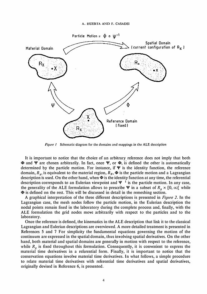
where t denotes time. These transformations present, as previously, non-vanishing jacobiansand are schematically represented in Figure 1.

3

Material Domain


Particle Motion = <I> o 14,1-1

Spatial Domain ( current configuration of Rx I

Reference Domain I fixed I

Figure I Schematic diagram for the domains and mappings in the ALE description

It is important to notice that the choice of an arbitrary reference does not imply that both (I) and 'I' are chosen arbitrarily. In fact, once 'I', or (I), is defined the other is automatically determined by the particle motion. For instance, if 'I' is the identity function, the reference domain, R

x, is equivalent to the material region, Rx, (I) is the particle motion and a Lagrangian

description is used. On the other hand, when (I) is the identity function at any time, the referential description corresponds to an Eulerian viewpoint and '1' 1 is the particle motion. In any case, the generality of the ALE formulation allows to prescribe 'I' in a subset of R

,. x [O, oo[ while

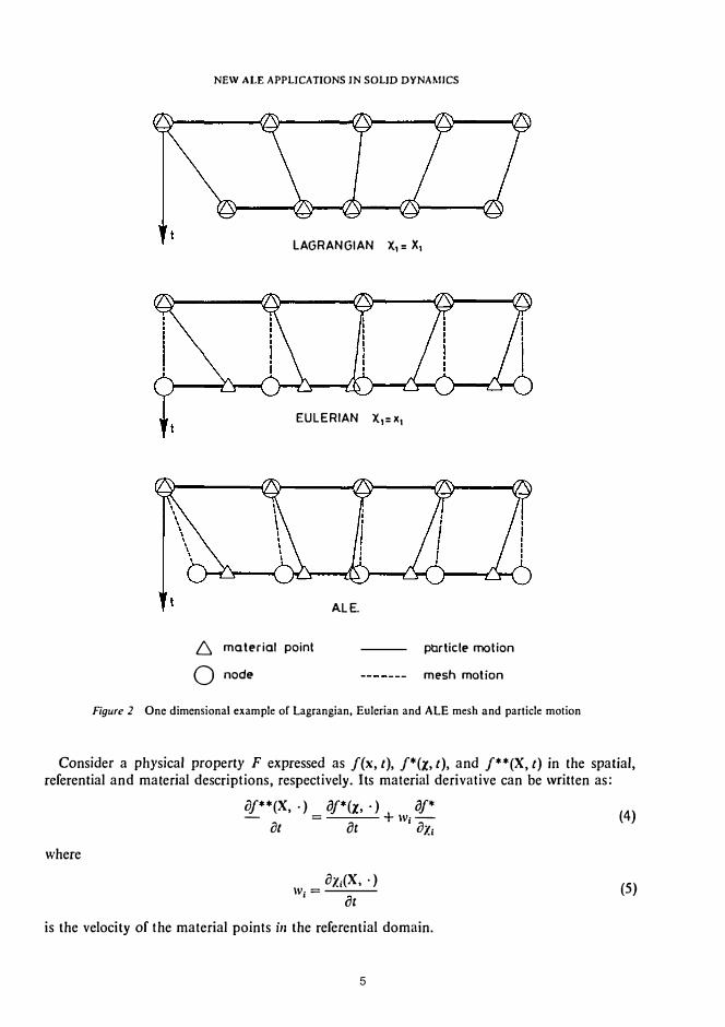
(I) is defined on the rest. This will be discussed in detail in the remeshing section. A graphical interpretation of the three different descriptions is presented in Figure 2. In the

Lagrangian case, the mesh nodes follow the particle motion, in the Eulerian description the nodal points remain fixed in the laboratory during the complete process and, finally, with the ALE formulation the grid nodes move arbitrarily with respect to the particles and to the laboratory.

Once the reference is defined, the kinematics in the ALE description that link it to the classical Lagrangian and Eulerian descriptions are overviewed. A more detailed treatment is presented in References 5 and 7 For simplicity the fundamental equations governing the motion of the continuum are expressed in the spatial domain, thus involving spatial derivatives. On the other hand, both material and spatial domains are generally in motion with respect to the reference, while R

x is fixed throughout this formulation. Consequently, it is convenient to express the

material time derivatives in a referential form. Finally, it is important to notice that the conservation equations involve material time derivatives. In what follows, a simple procedure to relate material time derivatives with referential time derivatives and spatial derivatives, originally devised in Reference 6, is presented.

4


LAGRANGIAN X, = X,

EULERIAN X,= x1

6 material point

Q node

A.LE.

particle motion

mesh motion

Figure 2 One dimensional example of Lagrangian, Eulerian and ALE mesh and particle motion

Consider a physical property F expressed as f(x, t), f*(x, t), and f**(X, t) in the spatial, referential and material descriptions, respectively. Its material derivative can be written as:

where

of**(X, . ) iJJ*(x, ·) iJf* - = +w;-iJt iJt axi

\Vi =

iJx;(X, ·)

ac

is the velocity of the material points in the referential domain.

(4)

(5)

5


The formal mathematical notation for time derivatives is usually substituted in the literature, since Donea5, by a more engineering type of notation. That is, given f(?,, t),

aJ(?., . ) =

aJIat at { (6)

meaning, that the partial derivative is taken "holding ?, fixed". This remark is important in order not to confuse this notation with the classical mathematical sense of I:, which is "particularized at?,". Moreover, to simplify the subsequent developments, the star notation used to distinguish the three configurations (spatial, referential, or material) will be dropped.

Equation (4) relates the material time derivative with the referential time derivative. However, spatial derivatives are desired instead of derivatives off with respect to X· Equation (4) is further simplified by means of the following definitions of material velocity, v, and mesh velocity, v:

and

vi = aa�t (7a)

D; =aa�t (7b)

respectively. If the physical property is the spatial coordinate x, (4) and (7) yield:

or

where

• ax;(8) V·=V·+W·-

I I

J a• Xi

(9)

(10)

is the convective velocity. While w is the material velocity in the reference, c is the relative velocity of the particles with respect to the mesh in the laboratory system. Finally, substituting (10) into (4) and using the chain rule, yields the classical relationship between the material timederivative, the referential time derivative and the spatial derivative:

!Ix = !Ix + c; ::; ( 11)

ALE formulation of the conservation laws

Under the ALE description, the conservation laws that govern the motion of the continuum are written, in strong form, as:

co11ti1111ity

(12a)

6


boundaries are "natural boundary conditions", and thus, they are automatically included in the weak, or variational form of (12).

However, if part of the boundary is composed of a material surface, then a mixture of both conditions is sometimes required 17

• Firstly, the conditions required on a material surface are:

(a) no particles can cross it, and(b) stresses must be continuous across the surface (if a net force is applied to a surface of zero

mass the acceleration is infinite).

And two types of material surfaces are usually present: free surfaces, and solid wall boundaries which may be frictionless or not.

Along a solid wall boundary the particle velocity is defined (or coupled to a structure system in fluid-structure interaction problems). The requirement that no particles can cross it, can be simply verified if w is prescribed equal to zero along that boundary, i.e. v = v from (8) which consists in defining the material surface as Lagrangian. However, this condition may be relaxed imposing only the necessary condition: w equal to zero along the normal to the boundary. The latter allows remeshing tangent to the boundary, the advantages of this type of relaxed boundary condition are evident in the pulling example shown later. The dynamic condition is automatically verified along rigid boundaries, but it presents the classical difficulties in fluid-structure interaction problems when compatibility at nodal level in velocities and stresses is required. An extensive discussion for this case is found in Reference 14.

Along the other type of material surface, i.e. free surface, problems arise because its position is unknown. Thus, the kinematic and dynamic conditions must be imposed and solved. The first one, the kinematic condition can be formalized as:

C·n.,,

= 0 (14)

in an Eulerian description. However, since the boundary is moving, its equivalent in referential form is preferred because the referential domain is fixed, namely:

w·nx = 0 (15)

where nx is the exterior normal to the referential domain. While the second one, the dynamic condition expresses the stress-free situation:

(16)

and, as mentioned earlier, it is directly taken into account by the weak formulation. In conclusion, free surface problems are the only ones that introduce a new equation, (15),

that must be verified along that boundary. It is obvious that this new equation has a strong influence on the remeshing techniques employed.

Equations of state

The initial boundary value problem is not defined until the state equations which reflect the behaviour of the continuum, are specified. Here two of such equations are needed, the first one relates temperature and density to energy:

e = e(p, 0) (17)

The second relates stress and/ or its derivatives to temperature, and velocity and/ or its derivatives. The latter constitutive relationship admits several formal representations, here only two of them are discussed. They include, however, most of the engineering materials in fluid or solid mechanics.

8


First of all, the Cauchy stress tensor is defined as a function of velocity, temperature and density fields:

a= s(O, p, v) (18)

For instance, any generalized Newtonian fluid, Bird et al.22, falls in this category because its constitutive relationship is written as:

(OV· OV·

)(J •• = pc'i

. + µ

_. + _J

I) I) !I !I UXj UX;

(19)

where c5,1 is the Kronecker delta; µ is the dynamic viscosity which is shear rate dependent; p isthe pressure which is uniquely determined by density and temperature for compressible fluids or by the velocity field for incompressible fluids. In any case, it is important to notice that ( 18) represents a class of no memory materials. Observe that the stress tensor is uniquely determined at each spatial point given the other instantaneous fields.

The other formal representation of the stress constitutive relationship is associated with path-dependent materials, or materials with memory. It relates the material time derivative of the Cauchy stress tensor with the same material fields as previously and with the stress field:

0(1

, - = r(O, p, v, a)ac x

(20)

Any of the frequently employed rate type constitutive equations may be written in the previous form. Therefore (20) models a wide range of solid materials and problems, going from small strain linear elasticity to strongly non-linear large strain elasto-plasticity. For instance, any hypo-elastic material can be defined as behaving in the following way:

(21)

where .1afi is the objective increment of stresses and represents the part of a due to actual straining of the material ("pure deformation"), i.e.:

(22)

C is the material response matrix which usually depends on the stress, a; v1k

,IJ are the components

of the velocity stretch tensor, vii.ii = � (ov; + ovi). The rest of the terms of (21) are associated2 OX) OX;

to the rotation of the stress tensor. Two formulations are usually employed, the Green-Naghdi formulation if W is taken as the rate of rotation matrix, or the more usual Zaremba-Jaumann-Noll or co-rotational formulation when Wis the spin tensor. In the latter,

1 (

OV· OV·)the components of W are simply v

1;,

11 = - -' - -1

• Usually, these terms associated to the2 ox

) OX;

rotation are written as:

(23a)

where

(23b)

9


The generalized fourth order tensor C which represents the material response, can be derived in terms of the Jaumann rate of the Cauchy stress tensor:

(24a)

or in terms of the Truesdell rate, as:

(24b)

In the previous equation the tensor C* is needed to insure the objectivity of C, and it is defined by:

(24c)

Finally, in order to be consistent with the ALE formulation the material time derivative in (21) is replaced by the referential one making use of (11), which yields:

auij' auij- = -Ck - + CijklV{k,I) + SiJUV[k,IJ at l axk

(25)

Notice that now, in opposition to (18), the constitutive equation must be integrated, and the decomposition of the stress rate in three terms, transport, pure deformation and the rotational part, should be exploited during the time integration.

The generalization to elasto-plastic materials is readily obtained by defining a yield surface and supposing that the strain rate is linearly separable into elastic and plastic components. It is very important to notice that the hardening rules which explicitly define the evolution of the yielding surface during plastic deformation, are usually written in incremental or rate form. That is, the yielding limit in isotropic hardening or the back stresses in the kinematic hardening are described by an equation such as (20), and consequently the same time integration algorithm is used for the stress tensor and related variables. Note also that (20) or (25) are not exclusive of path-dependent materials but Hookean linear elasticity, for instance, is also included. Consequently, an efficient integration algorithm for (25) can uniformly treat most of the structural mechanics problems.

Apart from physical considerations, this classification is also numericaJly sound, because the algorithms associated to ( 18) or to (20) are completely different; in fact, the classification is intrinsically related to the ALE formulation. Classically, the so-called phenomenological mathematical models represented by (18) where no updating is necessary, are used in fluid mechanics where an Eulerian formulation is usually employed. On the other hand, incremental constitutive relations are common in structural/solid mechanics and are normally associated to a Lagrangian formulation. The updating of any physical property in a Lagrangian description is simple because the reference follows the particles; while in the ALE or the Eulerian formulation such an update is much more involved. This explains why the ALE formulation was naturally developed in fluid mechanics and only recently it is applied in solid mechanics problems9

•10

•11

•12

.

Remeshing

The equations that must be solved are ( 12), (13 ), ( 17) and (18) or (20) but also (9) is necessary and therefore, the resolution is only possible if the mesh velocities are given in the domain. The remeshing techniques are concerned with the definition of v. For instance, if v = 0, the Eulerian description is imposed, but if v = vis prescribed, the Lagrangian description is used. It is obvious that finding the best choice for these velocities and a low cost algorithm for updating the mesh constitutes one of the major problems of the ALE description (cost meaning, here, computer time and computer storage).

10


As a consequence of the discussion on boundary conditions, two cases are considered. The first one assumes that all the boundaries of the domain have a known position at every instant, this includes Eulerian inflow /outflow boundaries, prescribed boundary motion of material surfaces and solid-wall boundaries. The second is associated to unknown free surfaces on the boundary of the domain (or material surfaces in general), and will be reduced to the former

once the position of the free surface is known. This means verifying the kinematic condition of the free surface, namely (14) or (15). These equations are readily verified if the material surface is defined as Lagrangian, i.e. e == w == O; this is useful in structural mechanics problems. However, in large boundary motion problems, the element size along these Lagrangian surfaces can induce prohibitive computer cost or numerical inaccuracy. Therefore a relaxed condition expressed by (14) and (15), is recommended, see also Huerta and Liu17• In this respect several important

remarks should be advanced:

• Equation (14) or (15) are defined along the material surface, therefore, these equations arenot solved in the complete domain but only along free surfaces. The extra equation inducedby the unknown position of the boundary is consequently less costly than the other fieldequations.

• The general formulation presented here does not describe the material surface with an elevation(over a datum level) parameter, thus vertical or folded surfaces (such as the ones present incoating flows or shell impact), for example, may be studied (see also the dam break problemin Huerta and Liu 7).

• Equations (14) and (15) are scalar and only relate mesh and particle motion normal to thematerial surface. This implies that the user has the choice of deciding the mesh motion alongthe material surface. This is referred to as mesh sliding along the boundary and has the

important advantage of precluding the use of pure Lagrangian nodes on these surfaces. Mostof the examples shown later make use of these remeshing features but in the pulling analysis theadvantages of such a procedure are clearly outlined. Finally, it should be noticed that thechoice between (14) or (15) obeys to numerical efficiency and user's preferences.

At this point, the case of unknown free surfaces is reduced to the one where all the boundariesof the domain are fixed or have a known prescribed motion. Therefore, the continuous remeshing is completely defined once � is given in the interior of the domain. This can be done by simple ad hoc formulae, using geometrical considerations18

, solving potential equations that maintain element regularity19•11, or any other mesh generation algorithms that conserve the elementconnectivity. Most of these remeshings are based on defining new locations for the nodes, and then computing the mesh velocities by finite difference approximation (i.e. increment of displacement over increment of time). If structured meshes are used, the authors recommend to use simple ad hoc formulae where the mesh velocity is linearly interpolated between the velocities at both ends of the inter-element lines. This is an extremely simple and efficient algorithm which maintains element regularity and it is obviously more cost effective than solving potential equations previous to the evaluation of the mesh velocities.

TIME INTEGRATION

In this section a brief discussion on the time integration schemes is presented. Keeping in mind the fast-transient dynamic context, the second order in time integration scheme presented in Reference 20 is generalized for the integration of the constitutive equation within the ALE formulation. After the finite element integration of the momentum equation, (12b), the system

11


of algebraic ordinary differential equations that must be integrated, is:

Ma = r••t - 11(v) - L f BTO' dx e Rt

(26)

where M is the mass matrix; a is the nodal acceleration vector; f••1 is the vector of externallyapplied loads; 11(v) is the convective vector (relative motion between mesh and particles); andthe last term is the internal force vector which is left as the sum of the element contributions.The element internal force vector is evaluated by means of the matrix of shape function derivatives,B, and the Cauchy stress tensor a.

Since an explicit scheme is sought, the mass matrix, M, is substituted by the lumped(diagonalized) mass matrix, ML, uncoupling the system defined by (26). Then the stabilitycondition must be enforced; it is associated to the minimum Courant number of equivalentlyto the maximum eigenvalue of the system. In fact, in clasto-plastic analysis, this stability conditionis related to the minimum element size and, as it will be shown in the numerical examples, theALE formulation is advantageous because it allows to maintain during the deformation processregular shaped elements.

On the other hand, the constitutive equation, (25) for elasto-plastic materials or (20) in general,must also be integrated. The finite element interpolation and integration for the stresses isdifferent from those of velocities or displacements. In fact, stresses arc needed at each quadraturepoint for further numerical integration of the internal work, see (26). In a similar manner toReference 11 a multiple stress collocation technique is used in the weak form, where the collocationpoints do coincide with the quadrature points 13• The induced system of algebraic equations isexplicit and trivial (the mass matrix coincides with the identity matrix), it may be written as:

f = r - 'la (27)

where f represents the vector of rate of stresses at the quadrature points, r is the Lagrangianstress rate which includes only the pure deformation and rotation part, while 'la is associatedto the transport of stresses, see (25).

As a matter of fact, a split-step algorithm is used to integrate in time this last system ofordinary differential equations. First of all, a pseudo-Lagrangian stress is obtained by simplyintegrating the Lagrangian stress rate, r; that is, assuming zero convective velocities. Then, the pseudo-Lagrangian stress is convected adding the contribution due to 'la· The particular expression for 'la depends on the time scheme employed, any numerical formulation for first order hyperbolic or conservation equations may be implemented. Here a Lax-Wendroff and aGodunov-type techniques were adopted to the particular nature of the stress fields (discontinuouselement to element) and the desired numerical constraints (explicit code) 13•

In order to maintain a central difference scheme for the time integration of (26) and (27), anuncoupled algorithm is devised. If accelerations are computed from (26) at time t" then velocitiesare evaluated at t•+ 1'2 by:

(28a)

Once the velocities are known at the half step, (27) is enforced. The stress rate is then computedat t•+ 112 and consequently stresses and displacements are simply updated by equations similarto the previous one, namely:

-r•+ 1 =

-r•-1 + .1ti'"+ 1/2 + @(.1£2)

d"+ 1 = dn-1 + .1tv•+ 1/2 + @(.1t2) (28b)

(28c)

12


With these new values, the right hand side term in (26) as well as the mass matrix can be

evaluated at ,n+ 1; thus, the acceleration is computed at the new time step (n + 1) and the process

repeated as many times as needed. The time scheme presented has the advantage that both conservation of momentum and the

constitutive equation are solved separately with the best suited technique in each case. For instance while simple updating techniques can be used in (26) if the relative motion of the mesh and the particles is small, on the contrary the stress (and stress related variables such as the yield stress) sensitivity to convection imposes sophisticated updating schemes. Moreover, as mentioned previously, the interest in interpolating the stresses directly at the quadrature points, precludes a simple coupling between the second order ordinary differential equations in (26) and the first order ones (27). Finally, such an algorithm allows second order accuracy and it is easily generalized to time partitioning computations. It must be noticed, however, that the second order accuracy is lost in variable time stepping computations.

NUMERICAL EXAMPLES

In this section the ALE formulation and the explicit time integration procedure are applied to several problems that range from purely academic test to engineering simulations. The first one is an elastic-plastic one-dimensional wave propagation problem first reported in Reference 9. This problem which has an obvious analytical solution in the elastic case allows to compare the numerical results with the exact solution. Moreover, the effectiveness of the formulation and in particular of the convection procedures, can be easily established.

The second example is the well known bar impact benchmark test. It is a classical test for impact codes and a full large strain demonstrative computation. It allows the comparison of Lagrangian and ALE results and presents a full range of boundary surfaces going from an axis of symmetry to free material surfaces with large boundary motion. A simple transformation of this example induces the following numerical simulation where necking appears and the effectiveness of the ALE formulation is demonstrated compared with the Lagrangian description.

Finally, an engineering example is shown. It simulates a coining process which is difficult and tedious to model a classical update Lagrangian description. However, it does not present any difficulty in the context of an ALE formulation and comparisons between a fast (dynamic) die velocity and a slow (quasi-static) die velocity are shown.

011e-dime11sio11al stress wave problem

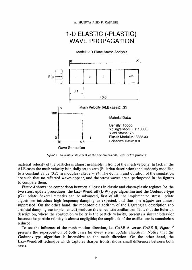
This elastic(-plastic) one-dimensional stress wave problem is presented here to assess the ALE formulation in the structural mechanics context. The material properties and element size are chosen equal to those used in Reference 9, for easier comparisons. Note, however, that the stress update schemes implemented here do not need special numerical parameters "a la" Streamline Upwind Petrov-Galerkin.

A schematic problem statement is shown in Figure 3, where the constants for the isotropic hardening material are given. The infinitely long elastic(-plastic) rod is discretized in 400 elements

of 0.1 size. The problem is assumed isothermal and constant density is supposed throughout. The propagation of a square compression stress wave (-100 in amplitude, 4.5 in width) is simulated under several descriptions: Lagrangian, Eulerian and ALE. For the latest two

arbitrarily chosen mesh velocities are imposed, one negative (CASE A) and one positive (CASE B). Since the purpose of this simulation is to provide a severe test to the formulation and the algorithms the mesh velocity is taken equal to one fourth of the speed of sound, notice that the

13


1-D ELASTIC (-PLASTIC)WAVE PROPAGATION

Model: 2-D Plane Stress Analysis

0 x

P{t) � l ' [ ' l ' [ . I�

�

0

.. � 40.0 -1

p Mesh Velocity (ALE cases): .25 100------,

0 10 4.5

Wave Generation

Material Data:

Density: 10000. Young's Modulus: 10000. Yield Stress: 75. Plastic Modulus: 3333.33 Poisson's Rat io: 0.0

Figure J Schematic statement of the one-dimensional slress wave problem

material velocity of the particles is almost negligible in front of the mesh velocity. In fact, in the ALE cases the mesh velocity is initially set to zero (Eulerian description) and suddenly modified to a constant value (0.25 in modulus) after t = 24. The domain and duration of the simulation are such that no reflected waves appear, and the stress waves are superimposed in the figures to compare them.

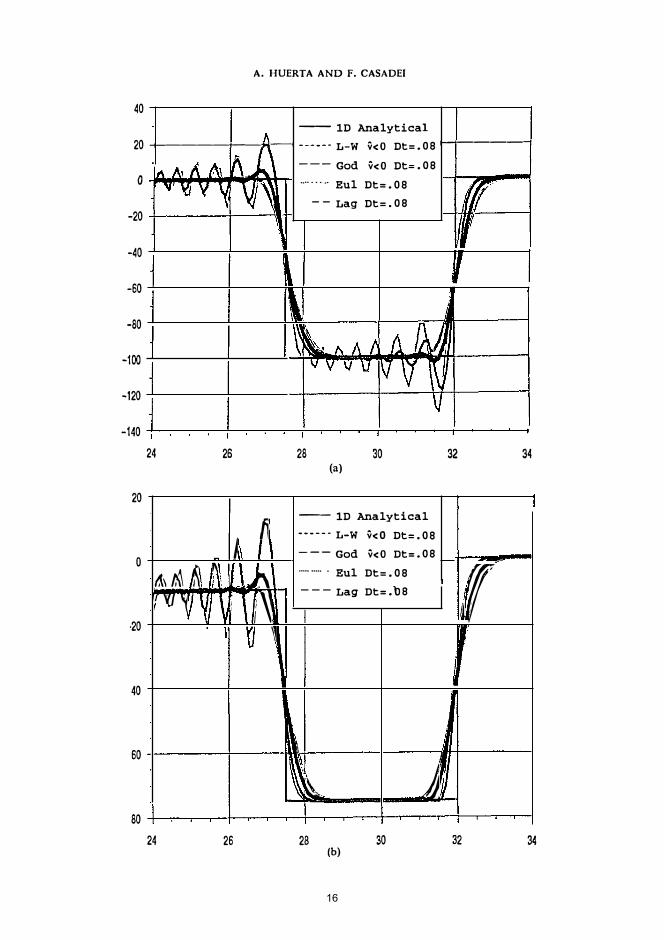
Figure 4 shows the comparison between all cases in elastic and elasto-plastic regimes for the two stress update procedures, the Lax-Wendroff (L-W) type algorithm and the Godunov-type (G) update. Several remarks can be advanced, first of all, the implemented stress updatealgorithms introduce high frequency damping, as expected, and thus, the ll'iggles are almostsuppressed. On the other hand, the monotonic algorithm of the Lagrangian description (noartificial damping was implemented) produces the unrealistic oscillations. Note that the Euleriandescription, where the convection velocity is the particle velocity, presents a similar behaviorbecause the particle velocity is almost negligible; the amplitude of the oscillations is nonethelessreduced.

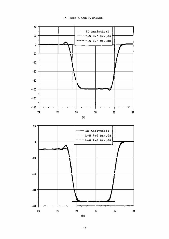
To see the influence of the mesh motion direction, i.e. CASE A versus CASE B, Figure 5 presents the superposition of both cases for every stress update algorithm. Notice that the Godunov-type algorithm is insensitive to the mesh direction. On the other hand, the Lax-Wendroff technique which captures sharper fronts, shows small differences between both cases.

14

NEW AI.E APPLICATIONS IN SOLID DYNAMICS

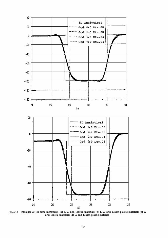
Finally, Figure 6 shows the influence of the time increment in the solution. As expected, the lower the Courant number the larger the relative phase error, in the L-W scheme. However, the solution is still very adequate since the dissipative character of the scheme damps out the shorter wavelengths. Note also that this time dependency is negligible in the Godunov-type of update.

Bar impact benchmark test

The bar impact problem is chosen here for several reasons: it is a standard benchmark problem for fast-transient dynamic computer codes, although no analytical solution exist the ALE results can be compared to the Lagrangian ones, and the advantages of the proposed formulation are clearly outlined.

A cylindrical bar of radius 3.2 mm and length 32.4 mm impacts a rigid frictionless wall at an initial velocity of 227 m/s. The material is assumed elasto-plastic with E = 117 Gpa, v = 0.350, a

>. 400 MPa, p = 8930 kg/m3, and a plastic modulus E

P = 100 MPa. The time-step is variable

and automatically chosen by the code to maintain the numerical stability, a maximum Courant number of 0.5 is imposed in the smaller element. An axisymmetric mesh of 250 bilinear elements is employed.

In Figure 7, the calculated deformed shapes for the Lagrangian (left) and ALE (right) descriptions are compared at every 10 µs (only the mesh is shown) up to the final 80 µs. Only the Godunov-type stress update algorithm is shown because negligible differences are found comparing with the Lax-Wendroff technique. The difference between the Lagrangian and ALE calculations for the radius and axial length are 0.5% and 0.4%, respectively.

Important differences, however, are observed in the time-step, !:J.t, employed, see Figure 8. The uniformity of the mesh, maintained by the Giuliani1 8 algorithm, allows larger and more uniform time increments. This obviously induces an important difference in the computer time required for the simulation. While the Lagrangian description needed 3 hours 44 min (31 700 time-steps), the ALE formulation used 27 min (1900 time-steps).

The adequacy of the stress updating algorithm is stressed in the last figure of this example. The distribution of final yield stress (directly related to the plastic strain) is plotted for the Lagrangian case and the ALE analysis. While Figure 9a shows a remarkable similarity between both simulation (observe that the contour lines are almost coincldent), Figure 9b shows important differences between the plastic zones at the final instant. In the latest case, no stress update procedure is implemented but the remeshing is performed. This is obviously a wrong calculation because no history dependent state variables are transported and the path-dependency is not reflected in the computations. However the height and width of the final bar present differences of only 1.3% and 6.5%, respectively, with the Lagrangian results. This suggests that the measures of final height and width are weak indicators of the goodness of the algorithm and that other results, such as the distribution of final yield stress, must be compared when dealing with this benchmark test.

Bar pulling and necking analysis

This example is a simple extension of the previous one. The same geometry and material are taken, even the same initial velocity is prescribed but now the sign is opposite. Thus the present example simulates a sort of pulling test. It has been chosen because it presents another possible advantage of the ALE formulation. While the Lagrangian analysis suffers from excessive element distortion, precisely where the necking occurs, the ALE description allows a regular element size distribution everywhere, see Figure 10. Figure 11 compares the yield stress distribution at

15

40

20

0

-20

-40

-60

-80

-100

-120

-140

20

0

·20

40

60

80


-- lD Analytical

-t-----t----w.---J ------ L-W v<O Dt=.08 t--t------i

24 26

) �

,1, � � �

� r, '{/ � I

/� �

24 26

--- God v<O Dt=. 08

····· · · ·· Eul Dt=.08

--Lag Dt=.08

28 30

(a)

-- lD Analytical

------ L-W v<O Dt=.08

--- God v<O Dt=.08

·········· · Eul Dt=.08

---Lag Dt=.08

i

� )J

28 30 (b)

32 34

jr '

32 34

16

-- lD Analytical

20 -+------,...--�---i ------ L-W bO Dt=.08 1-+------1

-God v>O Dt=,08

........ Eul Dt=. 08

--- Lag Dt=.08 -20 4------1----.... -L

-.-----�------'l-4-llllt---�

24 26 28 30 32

(c)

20

0

� -- lD Analytical

J -----· L-W v>O Dt=,08

--God V>O Dt=.08

Ad�� ............. Eul Dt=.08

rr I I'(/ � i�

--·- Lag Dt=.08

{ -20

l

It� j

-60

-8024· 28 30

(d)

Figure 4 Comparison between the obtained results, (a) CASE A (negative mesh velocity) with elastic material, {b) CASE A with elasto-plastic material, (c) CASE B (positive mesh velocity) with elastic material, (d) CASE B with

elasto-plastic material

17


40

-- lD Analytical

20 ··· ····· ·· L-W v<O Dt= .08

.A.. --- L-W v>O Dt=.08

0

-20

-40

-60

-so

-100

-120

-140

24 26 28 30 32 34

(a)

-- lD Analytical .. ..... L-W v<O Dt=.08

--- L-W v>O Dt=.08 0

-20

-40

\

)�

-60

-80

24 26 28 30 32 34

(b)

18

40

20

0

-20

-40

-60\

-80

-100

-120

140

24 26

24 26

-- lD Analytical ····· ·· God v<O Dt=.08

--- God v>O Dt=.08

I I

28 30

(c)

-- lD Analytical

God v<O Dt=.08

--- God bO

28 30

(d)

32

32

34

34

Figure 5 Influence of the mesh velocity direction on the stress update algorithms. (a) L-W and Elastic material; (b) L-W and Elasto-plastic material; (c) G and Elastic material; (d) G and Elasto-plastic material

19


40

-- lD Analytical

20 - ---- L-W v<O Dt=.08

--- L-W v>O Dt=.08 0

-20'

... ........ L-W v<O Dt=.04

r--- L-W v>O Dt=.04

-40

-60l

-80

-100

-120

-140

24 26 28 30 32

(a)

20

-- lD Analytical

------ L-W v<O Dt=.08

--- L-W v>O Dt=.08 . ... ..

.. L-W v<O Dt=.04

r""" 1 --- L-W v>O D�=.04

0

-20

-40

'� j

-60

-80

24 26 28 30 32 34

(b)

20

40

-- lD Analytical

20 ------ God v<O Dt=.08

--- God bO Dt=.08

0

\ ...

... God v<O Dt=,04

r--

God bO Dt=.04

I \ I

-20

-40

-60

J-80

-100

-120

-140

24 26 28 30 32 34

(c)

20

�- lD Analytical

------ God v<O Dt=.08

0

- God v>O Dt=.08

··············· God v<O Dt=.04

r --- God v>O Dt=.04

, I

-20

-40

' )\.

-60

-80

24 26 28 30 32 (d)

Figure 6 InHuence of the time increment. (a) L-W and Elastic material; (bl L-W and Elasto-plastic material; (c) G and Elastic material; (d) G and Elasto-plastic material

21


Initial (t = 0) t = 10 µs t= 20 t= 30 t = 40

t=50 t = 60 t= 70 t = BO

21 , O'U ,- ano 11LD1 -aa ._"-... ,a.11 ......... 11

Figure 7 Comparison between the deformed meshes obtained with the Lagrangian description (left) and ALE formulation (right)

c

Q)

E �

1E-7

g 1E-8

E

1 E-9 0

' --

ll. -

'

- - -

'

.... '\

A.,.

2E-5

-- - - - - - -

� -"6-..

-A-

-----

- - - -

- - -

Dt Lag. =>--

DtALE ,---

- - - - -

4E-5

Time

6E-5 8E-5

Figure 8 Variation of the time-increment, .1r, with time (during the deformation process)

22

lJOTES.

- 0

400

D

�:�� - -- _,

550-600

-

L

-0

MP a

CJ400 MPa-450

----, 500--- -·

-550-600

L

(a)

(b)

ALE

Fig11re 9 Comparison between nal yield stress distributions: (a) Lagrangian (left) and ALE (right); (b) Lagrangian (left) and incorrect computation without stress update during remeshing (right)

23


.

•!�� .

I

.

I

I

.

•

.

.

.

I •

I

I

u, ou .. nae t= 0 t=lOµs t =20 µs

Figure JO Pulling analysis: comparison of t he deformed meshes at various instants, Lagrangian (left)and ALE (right)

different instants and, obviously, the Lagrangian computation shows large inaccuracies due to the mesh distortion. It should be noticed, in this figure, that the free surface nodes are not defined as Lagrangian and that the remeshing allows tangential sliding of the mesh nodes along material surfaces even under large boundary motion.

Simulation of a forming process

Finally, an engineering problem is presented, a similar example is presented in Reference 21 but in a static analysis. It consists in an elasto-plastic material with E = 200 GPa, v = 0.30, u,. = 250 MPa, p = 8930kg/m3, and a plastic modulus E

P = lGPa. The body is deformed by

a rigid frictionless tool with a prescribed velocity, only a quarter of the domain (a rectangular region of 3 cm by 1 cm) is studied because two axes of symmetry are supposed, and a plane strain analysis is conducted using 2 x 2 Gauss integration. The analysis is performed up to a 60% reduction in height of the original piece. A schematic statement of this problem is presented in Figure I 2.

Note that the frictionless boundary condition is rather difficult to implement in the Lagrangian case. Moreover, different meshes are needed (see, for instance, Ref ere nee 21) depending on the

24

0 -400-450-500- ---,

----· 550•soo-

L

MP a

0 -400 MPa-450•500----1 - --· 550•soo-

L

Lag. ALE

"'· t= 10 µs

t= 20 µs

Figure 11 Pulling analysis: comparison between yield stress distributions

(a)

t= 20 µs

(b)

25

0 C\I


Symmetric Coining Model: 2-D Plane Strain Analysis

� 24

I Discretized

Rigid Punch

_.,d

(t) · Reg�on

- -,-rt--t-t--t---+-+" -t--t--t--t-1 =t=

6mm

0

�---+-+-+--l-+-t--t--t-12.5 • .................................. ._.__._...._........, _ _._..._...._......_..

l• 6 0mm_ j d(t)

T [ms] v [m/s]

t -----·

T

40.00

2.00

0.10

0.02

0.15

3.00

60.00

300.00

Figure 12 Schematic statement of the symmetric coining problem

reduction required because every reduction induces different deformations and consequently, diverse element distortions. And finally, the Lagrangian description needs an ad hoc mesh, particularly refined under the edge of the tool where most of the deformation occurs.

Figure 13 shows the evolution of the yield stress (equivalent plastic strain) during the deformation process for a punching velocity of 60 m/s. The ALE formulation allows to maintain element regularity and an accurate description of the boundary motion. The evolution of the plastic areas are always leaded by the right comer of the tool. Notice however that as expected, a plastic band is clearly detected between the previously mentioned corner and the center of the specimen.

To compare the influence of the dynamic effects different punch velocities are studied. Figure 14 shows the comparison between the final deformed shapes. The influence of the dynamic effects is negligible for die velocities under 3 m/s; but, as expected, the fast velocity cases induce a larger back extrusion while the quasi-static simulations allow larger amount of material to flow outward. The external free surface shape is clearly dependent on the dynamic effects.

26

Lt,lTB..

- 0

D 550 Mpa

llil 850-, 1150

�1450-1750

L.

NEW ALE APPUCATIONS IN SOLlO DYNAMICS

I I I

Initial

48%

: P:.'tl'nVM 31 CA.A� JrU': £1.il. � td.tn lm !ti�

12 % height reduction

Figure 13 Evolution of the yield stress field during the deformation process, die velocity of 60 m/s

SUMMARY AND CONCLUSIONS

The general overview and summarized discussion of the ALE formulation presented here indicates the applicability and effectiveness of this technique in generalized continuum mechanics problems. The applications shown are focussed in non-linear solid mechanics because the ALE formulation is already well expounded in the hydrodynamic and fluid-structure interaction fields.

This technique enhances the basic advantages of the finite element method for modelling complex geometries and boundary conditions. It allows a uniform and simple treatment of both confined boundaries and large boundary motion of free surfaces, as well as an excellent flexibility in moving the computational mesh. The result is a very versatile modelling technique which permits accommodation of large continuum distortion and boundary motion, numerical efficiency (from a computational cost point of view}, and accurate numerical modelling in particular on material surfaces mapping and interpolation enrichment over determined areas.

After the introduction to the ALE notation and fundamentals, a discussion of the primary governing issues has been presented. Kinematics which are the fundamental concern in ALE, are necessary to develop the governing equations of the continuum problem. Then several specific and inherent concerns of the ALE technique, boundary conditions implementation for large boundary motion, equations of state, and remeshing are discussed. Their adeQuate

27


lt..ICE • \IRSICt-1 00 �

Ol.l..B.RS FCtF1 LA C(t,F'OS,.lffit.

""' ""' 7

""""

-0 v= 0.15 mis

-550 Mpa

-850

---- 1150

-14501750

-

• c.a:o • D..10%.o-OS

Lv = 300 mis

Figure /4 Comparison between the final deformed meshes and yield stress distributions at different punching velocities

implementation is crucial for the applicability and effectiveness of the proposed technique; thus the discussion focusses on their advantages and drawbacks. All of the previous remarks are general in the ALE formulation, while the time integrationl algorithm employed is especially designed for the implementation of the ALE formulation in a fast-transient dynamics code.

Finally, it is important to notice that the numerical examples shown range from purely academic tests to real engineering simulations. They show the applicability of this formulation

to non-linear solid mechanics and in particular to impact, coining or forming analysis.

ACKNOWLEDGEMENTS

The first author takes this chance to acknowledge the Applied Mechanics Division, at the Joint Research Centre in lspra where this work was developed, for his appointment as visiting scientist. The authors want also to express their deep appreciation to J. Donea for his invaluable and

helpful suggestions through long anf fruitful technical discussions.

REFERENCES

Noh, W. F. CEL: A time-dependent tY.o-space-dimensional coupled Eulerian-Lagrangian code, Me1h. in Comp. Phys., 3 (Eds. B. Alder, S. Fernbach and M. Rotenberg), Academic Press, New York (1964)

2 Pracht, W. E. Calculating three-dimensional fluid flows at all flow speeds with an Eulerian-Lagrangian computing mesh, J of Comp Phys 17, 132-159 (1975)

28

new ale applications in non-linear fast-transient …

Documents