new ahp methods for handling uncertainty within the belief function theory
DESCRIPTION
As society becomes more complex, people are faced with many situations in which they have to make a decision among different alternatives. However, the most preferable one is not always easily selected.TRANSCRIPT
UNIVERSITE DE TUNIS
INSTITUT SUPERIEUR DE GESTION
THESE EN COTUTELLE
en vue de l’obtention du titre de docteur en
INFORMATIQUE DE GESTION
GENIE INFORMATIQUE ET AUTOMATIQUE
NEW AHP METHODS FOR HANDLING UNCERTAINTY
WITHIN THE BELIEF FUNCTION THEORY
AMEL ENNACEUR
SOUTENUE LE 29 MAI 2015, DEVANT LE JURY COMPOSE DE:NAHLA BEN AMOR PROFESSEUR, UNIVERSITE DE TUNIS PRESIDENT
ARNAUD MARTIN PROFESSEUR, UNIVERSITE DE RENNES 1 RAPPORTEUR
ALLEL HADJALI PROFESSEUR, ENSMA RAPPORTEUR
LAURENT DELAHOCHE MAITRE DE CONFERENCES-HDR, UNIVERSITE DE PICARDIE EXAMINATEUR
GILLES GONCALVES PROFESSEUR, UNIVERSITE D’ARTOIS INVITE
ZIED ELOUEDI PROFESSEUR, UNIVERSITE DE TUNIS DIRECTEUR DE THESE
ERIC LEFEVRE PROFESSEUR, UNIVERSITE D’ARTOIS DIRECTEUR DE THESE
Ecole doctorale : Institut Superieur de Gestion Tunis
Laboratoire/Unite de recherche : LARODEC/LGI2A


Acknowledgements
In some ways, this is the most difficult section to write. There are so many people who haveprovided me with their support during the achievement of my PhD, and it is not easy to find theright words to express my gratitude.
My sincere thanks to my supervisors, Pr. Zied Elouedi (University of Tunis, Tunisia) andPr. Eric Lefevre (University of Artois, France), who without any hesitation, accepted me as theirPhD student. From that time forward, they offered me so much advice and patiently supervisedme. I have learned a lot from them, without their help I could not have finished my dissertationsuccessfully. It is not sufficient to express my gratitude with only a few words.
My thanks go to all members of my laboratory LARODEC at Institut Superieur de Gestionde Tunis and all members of my laboratory LGI2A at University of Artois.
Most importantly, none of this would have been possible without the love and patience of myparents. They have been a constant source of love, concern, support and strength all these years.To them, I dedicate this work.
I have to give a special mention for the support given by my husband. I warmly appreciatehis generosity and understanding. Finally, I would like to express my heart-felt gratitude to mybrother, my sister in law and my lovely son.
Contents
Introduction 1
I Theoretical Aspects 6
1 Multi-Criteria Decision Making: An overview 7
1.1 Introduction . . . . . . . . . . . . . . . . . . . . . . . . . . . . . . . . . . . . . 7
1.2 Multi-Criteria Decision Making . . . . . . . . . . . . . . . . . . . . . . . . . . 8
1.2.1 Basic concepts . . . . . . . . . . . . . . . . . . . . . . . . . . . . . . . 8
1.2.2 Decision making process . . . . . . . . . . . . . . . . . . . . . . . . . . 10
1.3 Classification of MCDM methods . . . . . . . . . . . . . . . . . . . . . . . . . 12
1.4 Analytic Hierarchy Process as a MCDM method . . . . . . . . . . . . . . . . . . 15
1.4.1 AHP hierarchy . . . . . . . . . . . . . . . . . . . . . . . . . . . . . . . 15
1.4.2 Pair-wise comparison . . . . . . . . . . . . . . . . . . . . . . . . . . . . 16
1.4.3 Consistency ratio . . . . . . . . . . . . . . . . . . . . . . . . . . . . . . 17
ii
CONTENTS iii
1.4.4 Priority vectors and synthetic utility . . . . . . . . . . . . . . . . . . . . 18
1.5 Illustrative example . . . . . . . . . . . . . . . . . . . . . . . . . . . . . . . . . 18
1.5.1 Determining Weights of Criteria . . . . . . . . . . . . . . . . . . . . . . 19
1.5.2 Determining priorities of alternatives with respect to criteria . . . . . . . 21
1.5.3 Synthetic utility . . . . . . . . . . . . . . . . . . . . . . . . . . . . . . . 22
1.6 Advantages and limits of AHP method . . . . . . . . . . . . . . . . . . . . . . . 23
1.7 Conclusion . . . . . . . . . . . . . . . . . . . . . . . . . . . . . . . . . . . . . 24
2 AHP method under uncertainty 25
2.1 Introduction . . . . . . . . . . . . . . . . . . . . . . . . . . . . . . . . . . . . . 25
2.2 AHP method under uncertainty . . . . . . . . . . . . . . . . . . . . . . . . . . . 26
2.2.1 Brief refresher on Probabilistic AHP . . . . . . . . . . . . . . . . . . . . 26
2.2.2 Brief refresher on fuzzy AHP . . . . . . . . . . . . . . . . . . . . . . . 27
2.3 Belief function theory . . . . . . . . . . . . . . . . . . . . . . . . . . . . . . . . 30
2.3.1 Basic concepts . . . . . . . . . . . . . . . . . . . . . . . . . . . . . . . 30
2.3.2 Basic tools . . . . . . . . . . . . . . . . . . . . . . . . . . . . . . . . . 35
2.3.3 Decision making . . . . . . . . . . . . . . . . . . . . . . . . . . . . . . 39
2.3.4 Uncertainty Measures . . . . . . . . . . . . . . . . . . . . . . . . . . . 40
2.3.5 Multi-variable operations . . . . . . . . . . . . . . . . . . . . . . . . . . 42
2.3.6 MCDM under the belief function theory . . . . . . . . . . . . . . . . . . 45
2.4 AHP method under the belief function framework . . . . . . . . . . . . . . . . . 46
2.4.1 DS/AHP approach . . . . . . . . . . . . . . . . . . . . . . . . . . . . . 47

CONTENTS iv
2.4.2 Utkin method . . . . . . . . . . . . . . . . . . . . . . . . . . . . . . . . 51
2.4.3 ER-MCDM method . . . . . . . . . . . . . . . . . . . . . . . . . . . . 52
2.4.4 TIN-DS/AHP method . . . . . . . . . . . . . . . . . . . . . . . . . . . 54
2.5 Conclusion . . . . . . . . . . . . . . . . . . . . . . . . . . . . . . . . . . . . . 55
II Contributions 57
3 Modeling dependency between alternatives and criteria 58
3.1 Introduction . . . . . . . . . . . . . . . . . . . . . . . . . . . . . . . . . . . . . 58
3.2 Belief AHP method . . . . . . . . . . . . . . . . . . . . . . . . . . . . . . . . . 59
3.2.1 Introduction . . . . . . . . . . . . . . . . . . . . . . . . . . . . . . . . . 59
3.2.2 Computational procedure . . . . . . . . . . . . . . . . . . . . . . . . . . 60
3.3 A new belief AHP extension . . . . . . . . . . . . . . . . . . . . . . . . . . . . 68
3.3.1 Modeling dependency between alternatives and criteria . . . . . . . . . . 68
3.3.2 A new aggregation process using the belief function framework . . . . . 69
3.4 Computational experiments . . . . . . . . . . . . . . . . . . . . . . . . . . . . . 74
3.4.1 Evaluation algorithm . . . . . . . . . . . . . . . . . . . . . . . . . . . . 75
3.4.2 Simulation algorithm . . . . . . . . . . . . . . . . . . . . . . . . . . . . 76
3.4.3 Simulation results . . . . . . . . . . . . . . . . . . . . . . . . . . . . . 78
3.4.4 Comparison with DS/AHP method . . . . . . . . . . . . . . . . . . . . . 81
3.4.5 Catering selection problem . . . . . . . . . . . . . . . . . . . . . . . . . 82
3.5 Conclusion . . . . . . . . . . . . . . . . . . . . . . . . . . . . . . . . . . . . . 85
CONTENTS v
4 A new ranking procedure by belief pair-wise comparisons 87
4.1 Introduction . . . . . . . . . . . . . . . . . . . . . . . . . . . . . . . . . . . . . 87
4.2 Limits of Saaty scale . . . . . . . . . . . . . . . . . . . . . . . . . . . . . . . . 88
4.3 A pair-wise comparison process: A new elicitation technique . . . . . . . . . . . 89
4.3.1 Pair-wise comparison matrix with belief distributions . . . . . . . . . . . 89
4.3.2 Special cases . . . . . . . . . . . . . . . . . . . . . . . . . . . . . . . . 92
4.3.3 A new consistency index . . . . . . . . . . . . . . . . . . . . . . . . . . 93
4.4 Yes-No/AHP: A new aggregation process using the “yes” or “no” framework . . 93
4.4.1 Identification of the candidate criteria and alternatives . . . . . . . . . . 94
4.4.2 Computing the weight of considered criteria . . . . . . . . . . . . . . . . 94
4.4.3 Computing the alternatives priorities . . . . . . . . . . . . . . . . . . . . 95
4.4.4 Updating the alternatives priorities . . . . . . . . . . . . . . . . . . . . . 97
4.4.5 Decision making . . . . . . . . . . . . . . . . . . . . . . . . . . . . . . 99
4.5 Handling dependency between alternatives and criteria under Yes-No/AHP method100
4.6 Experimental analysis . . . . . . . . . . . . . . . . . . . . . . . . . . . . . . . . 101
4.6.1 Simulation algorithm . . . . . . . . . . . . . . . . . . . . . . . . . . . . 101
4.6.2 Simulation results . . . . . . . . . . . . . . . . . . . . . . . . . . . . . 103
4.6.3 Catering selection problem . . . . . . . . . . . . . . . . . . . . . . . . . 106
4.7 Conclusion . . . . . . . . . . . . . . . . . . . . . . . . . . . . . . . . . . . . . 108
5 Constructing belief functions from qualitative expert assessments 109
5.1 Introduction . . . . . . . . . . . . . . . . . . . . . . . . . . . . . . . . . . . . . 109
CONTENTS vi
5.2 Motivations . . . . . . . . . . . . . . . . . . . . . . . . . . . . . . . . . . . . . 110
5.3 Binary Relations and Preference Modeling . . . . . . . . . . . . . . . . . . . . . 111
5.4 Overview of qualitative reasoning methods . . . . . . . . . . . . . . . . . . . . . 113
5.4.1 Wong and Lingras’ Method . . . . . . . . . . . . . . . . . . . . . . . . 113
5.4.2 Parsons Method . . . . . . . . . . . . . . . . . . . . . . . . . . . . . . . 114
5.4.3 Bryson Method . . . . . . . . . . . . . . . . . . . . . . . . . . . . . . . 114
5.4.4 Ben Yaghlane et al.’s Method . . . . . . . . . . . . . . . . . . . . . . . . 115
5.5 A new elicitation method using qualitative assessments . . . . . . . . . . . . . . 117
5.5.1 Preference articulation: Incompleteness . . . . . . . . . . . . . . . . . . 117
5.5.2 Preference articulation: Incomparability . . . . . . . . . . . . . . . . . . 117
5.5.3 Preference articulation: Weak preference relation . . . . . . . . . . . . . 124
5.5.4 A global model in the presence of different relations . . . . . . . . . . . 130
5.6 Conclusion . . . . . . . . . . . . . . . . . . . . . . . . . . . . . . . . . . . . . 130
6 AHP method based on belief preference relations 131
6.1 Introduction . . . . . . . . . . . . . . . . . . . . . . . . . . . . . . . . . . . . . 131
6.2 On the extraction of scores from qualitative pair-wise comparison matrices . . . . 132
6.3 AHP method with belief preference relations . . . . . . . . . . . . . . . . . . . 135
6.3.1 Qualitative AHP method . . . . . . . . . . . . . . . . . . . . . . . . . . 135
6.3.2 Identification of the candidate criteria and alternatives . . . . . . . . . . 136
6.3.3 Computing the weight of considered criteria . . . . . . . . . . . . . . . . 136
6.3.4 Computing and updating the alternatives priorities . . . . . . . . . . . . 137
CONTENTS vii
6.3.5 Decision making . . . . . . . . . . . . . . . . . . . . . . . . . . . . . . 138
6.4 Introducing dependency under qualitative AHP method: Conditional qualitativeAHP . . . . . . . . . . . . . . . . . . . . . . . . . . . . . . . . . . . . . . . . . 139
6.5 Experimental analysis . . . . . . . . . . . . . . . . . . . . . . . . . . . . . . . . 140
6.5.1 Simulation algorithm . . . . . . . . . . . . . . . . . . . . . . . . . . . . 140
6.5.2 Simulation results . . . . . . . . . . . . . . . . . . . . . . . . . . . . . 142
6.5.3 Catering selection problem . . . . . . . . . . . . . . . . . . . . . . . . . 144
6.6 Conclusion . . . . . . . . . . . . . . . . . . . . . . . . . . . . . . . . . . . . . 145
Conclusion 147
A Experimental results 152
A.1 Introduction . . . . . . . . . . . . . . . . . . . . . . . . . . . . . . . . . . . . . 152
A.2 Experimental analysis . . . . . . . . . . . . . . . . . . . . . . . . . . . . . . . . 152
A.3 Conclusion . . . . . . . . . . . . . . . . . . . . . . . . . . . . . . . . . . . . . 155
B Sensitivity analysis 156
B.1 Introduction . . . . . . . . . . . . . . . . . . . . . . . . . . . . . . . . . . . . . 156
B.2 Mathematical methods . . . . . . . . . . . . . . . . . . . . . . . . . . . . . . . 157
B.3 Statistical methods . . . . . . . . . . . . . . . . . . . . . . . . . . . . . . . . . 157
B.4 Graphical methods . . . . . . . . . . . . . . . . . . . . . . . . . . . . . . . . . 158
B.5 Conclusion . . . . . . . . . . . . . . . . . . . . . . . . . . . . . . . . . . . . . 159
References 160
List of Figures
1.1 Decision making steps . . . . . . . . . . . . . . . . . . . . . . . . . . . . . . . 12
1.2 The main MCDM families . . . . . . . . . . . . . . . . . . . . . . . . . . . . . 13
1.3 Hierarchy of car choice AHP model . . . . . . . . . . . . . . . . . . . . . . . . 19
2.1 Hierarchy of modified car choice model . . . . . . . . . . . . . . . . . . . . . . 48
2.2 Decision problem related to avalanche risk zoning (Tacnet et al., 2010) . . . . . . 54
2.3 The corresponding TIN knowledge matrices . . . . . . . . . . . . . . . . . . . . 55
3.1 The general decision-making paradigm based on the belief AHP . . . . . . . . . 60
3.2 The belied AHP Hierarchy of car choice model . . . . . . . . . . . . . . . . . . 62
3.3 A new aggregation process . . . . . . . . . . . . . . . . . . . . . . . . . . . . . 65
3.4 Ranking of alternatives using Belief AHP . . . . . . . . . . . . . . . . . . . . . 67
3.5 The general decision-making paradigm based on the conditional belief AHP . . . 69
3.6 The new aggregation procedure under the conditional belief AHP method . . . . 70
3.7 Ranking of alternatives using conditional belief AHP . . . . . . . . . . . . . . . 74
viii
LIST OF FIGURES ix
3.8 Simulation algorithm steps . . . . . . . . . . . . . . . . . . . . . . . . . . . . . 76
3.9 Percentage of contradiction (%) based on 3 alternatives . . . . . . . . . . . . . . 78
3.10 Percentage of contradiction (%) based on 6 alternatives . . . . . . . . . . . . . . 79
3.11 Percentage of contradiction (%) based on 9 alternatives . . . . . . . . . . . . . . 79
3.12 Percentage of contradiction (%) based on 3 criteria . . . . . . . . . . . . . . . . 80
3.13 Percentage of contradiction (%) based on 10 criteria . . . . . . . . . . . . . . . . 80
3.14 Comparison of AHP extensions according to the percentage of contradiction(based on 3 alternatives) . . . . . . . . . . . . . . . . . . . . . . . . . . . . . . 81
3.15 Comparison of AHP extensions according to the percentage of contradiction(based on 6 alternatives) . . . . . . . . . . . . . . . . . . . . . . . . . . . . . . 81
3.16 Comparison of AHP extensions according to the percentage of contradiction(based on 9 alternatives) . . . . . . . . . . . . . . . . . . . . . . . . . . . . . . 82
3.17 Hierarchy of catering firm selection problem . . . . . . . . . . . . . . . . . . . . 83
3.18 Sensitivity analysis of Hygiene criterion . . . . . . . . . . . . . . . . . . . . . . 84
3.19 Sensitivity analysis of Quality of meal criterion . . . . . . . . . . . . . . . . . . 85
4.1 Belief pair-wise comparison technique . . . . . . . . . . . . . . . . . . . . . . . 91
4.2 The general decision-making paradigm based on Yes-No/AHP . . . . . . . . . . 94
4.3 The resulting contribution of Yes-No/AHP . . . . . . . . . . . . . . . . . . . . . 100
4.4 The general decision-making paradigm based on conditional Yes-No/AHP . . . . 100
4.5 Percentage of contradiction (%) based on 5 alternatives . . . . . . . . . . . . . . 104
4.6 Percentage of contradiction (%) based on 7 alternatives . . . . . . . . . . . . . . 104
4.7 Percentage of contradiction (%) based on 9 alternatives . . . . . . . . . . . . . . 105
LIST OF FIGURES x
4.8 Percentage of contradiction (%) based on 5 criteria . . . . . . . . . . . . . . . . 105
4.9 Sensitivity analysis of Hygiene criterion . . . . . . . . . . . . . . . . . . . . . . 107
4.10 Sensitivity analysis of Quality of meal criterion . . . . . . . . . . . . . . . . . . 107
5.1 Belief relations built from thresholds and crisp scores. . . . . . . . . . . . . . . . 127
6.1 The general decision-making paradigm based on qualitative AHP . . . . . . . . . 136
6.2 The general decision-making paradigm based on conditional qualitative AHP . . 139
6.3 Percentage of contradiction (%) based on 3 alternatives . . . . . . . . . . . . . . 142
6.4 Percentage of contradiction (%) based on 10 alternatives . . . . . . . . . . . . . 143
6.5 Percentage of contradiction (%) based on 10 criteria . . . . . . . . . . . . . . . . 143
6.6 Sensitivity analysis of Hygiene criterion . . . . . . . . . . . . . . . . . . . . . . 144
6.7 Sensitivity analysis of Quality of meal criterion . . . . . . . . . . . . . . . . . . 145
6.8 A Summary of the whole work . . . . . . . . . . . . . . . . . . . . . . . . . . . 149
List of Tables
1.1 A Typical decision matrix . . . . . . . . . . . . . . . . . . . . . . . . . . . . . . 9
1.2 Decision matrix . . . . . . . . . . . . . . . . . . . . . . . . . . . . . . . . . . . 10
1.3 A comparative table of MCDM methods . . . . . . . . . . . . . . . . . . . . . . 14
1.4 The Saaty Rating Scale . . . . . . . . . . . . . . . . . . . . . . . . . . . . . . . 17
1.5 Average random index (RI) . . . . . . . . . . . . . . . . . . . . . . . . . . . . 18
1.6 Pair-wise comparisons of criteria . . . . . . . . . . . . . . . . . . . . . . . . . . 19
1.7 Pair-wise comparison matrix . . . . . . . . . . . . . . . . . . . . . . . . . . . . 20
1.8 Normalized Pair-wise comparison matrix . . . . . . . . . . . . . . . . . . . . . 20
1.9 Computing the criteria priority values . . . . . . . . . . . . . . . . . . . . . . . 20
1.10 Comparison matrix for Style Criterion . . . . . . . . . . . . . . . . . . . . . . . 21
1.11 Comparison matrix for Reliability Criterion . . . . . . . . . . . . . . . . . . . . 21
1.12 Comparison matrix for Fuel Criterion . . . . . . . . . . . . . . . . . . . . . . . 22
1.13 Comparison matrix for Price Criterion . . . . . . . . . . . . . . . . . . . . . . . 22
1.14 Alternatives priority matrix . . . . . . . . . . . . . . . . . . . . . . . . . . . . . 22
xi
LIST OF TABLES xii
1.15 The global priority matrix . . . . . . . . . . . . . . . . . . . . . . . . . . . . . . 23
2.1 The fuzzy Saaty scale . . . . . . . . . . . . . . . . . . . . . . . . . . . . . . . . 28
2.2 Example of bbas expressed on the frame of discernment Θ . . . . . . . . . . . . 33
2.3 Knowledge/favourable scale . . . . . . . . . . . . . . . . . . . . . . . . . . . . 47
2.4 Criteria priority values . . . . . . . . . . . . . . . . . . . . . . . . . . . . . . . 49
2.5 Initial pair-wise matrix for Comfort criterion . . . . . . . . . . . . . . . . . . . . 49
2.6 Pair-wise matrix for Comfort criterion after influence of its priority rating . . . . 49
2.7 Pair-wise matrix for Price, Fuel and Style . . . . . . . . . . . . . . . . . . . . . 50
2.8 Priority values . . . . . . . . . . . . . . . . . . . . . . . . . . . . . . . . . . . . 50
2.9 The bba mcar after combining all evidence . . . . . . . . . . . . . . . . . . . . . 50
2.10 Belief and plausibility values for subsets of cars . . . . . . . . . . . . . . . . . . 51
2.11 Expert preferences related to criteria . . . . . . . . . . . . . . . . . . . . . . . . 52
3.1 The weights assigned to the criteria according to the expert’s opinion . . . . . . . 62
3.2 Comparison matrix for Price criterion . . . . . . . . . . . . . . . . . . . . . . . 63
3.3 Priorities values . . . . . . . . . . . . . . . . . . . . . . . . . . . . . . . . . . . 65
3.4 The measure of reliability . . . . . . . . . . . . . . . . . . . . . . . . . . . . . . 66
3.5 The bba mcar after combining all evidence . . . . . . . . . . . . . . . . . . . . . 66
3.6 Vacuous extension of bba . . . . . . . . . . . . . . . . . . . . . . . . . . . . . . 71
3.7 Ballooning extension of conditional bba . . . . . . . . . . . . . . . . . . . . . . 72
3.8 The obtained bba: mΘ×Ω . . . . . . . . . . . . . . . . . . . . . . . . . . . . . . 73
3.9 The obtained bba: mΘ×Ω↓Θ . . . . . . . . . . . . . . . . . . . . . . . . . . . . . 74
LIST OF TABLES xiii
3.10 The Final ranking of alternative . . . . . . . . . . . . . . . . . . . . . . . . . . . 74
3.11 Decision matrix . . . . . . . . . . . . . . . . . . . . . . . . . . . . . . . . . . . 77
3.12 The preference relations matrices . . . . . . . . . . . . . . . . . . . . . . . . . . 77
3.13 Decision matrix . . . . . . . . . . . . . . . . . . . . . . . . . . . . . . . . . . . 84
4.1 The weights preferences assigned to the criteria according to the expert’s opinion 92
4.2 Belief pair-wise matrix: Partial combination . . . . . . . . . . . . . . . . . . . . 92
4.3 Belief pair-wise matrix: pignistic probabilities . . . . . . . . . . . . . . . . . . . 95
4.4 Belief pair-wise matrix regarding c1 criterion . . . . . . . . . . . . . . . . . . . 96
4.5 Belief pair-wise matrix regarding c1 criterion . . . . . . . . . . . . . . . . . . . 96
4.6 Belief pair-wise matrix regarding c1 criterion . . . . . . . . . . . . . . . . . . . 97
4.7 The bbas mc2 , mc3 and mc4 . . . . . . . . . . . . . . . . . . . . . . . . . . . . . 97
4.8 The bbas mc2,c3 and mαc2,c3c2,c3 . . . . . . . . . . . . . . . . . . . . . . . . . . . . . 98
4.9 The bbas mαc1c1 and mαc4
c4 after discounting . . . . . . . . . . . . . . . . . . . . . 99
4.10 The overall bba . . . . . . . . . . . . . . . . . . . . . . . . . . . . . . . . . . . 99
4.11 The final result using the Yes-No/AHP approach . . . . . . . . . . . . . . . . . . 99
4.12 Decision matrix . . . . . . . . . . . . . . . . . . . . . . . . . . . . . . . . . . . 102
4.13 The preference relations matrices . . . . . . . . . . . . . . . . . . . . . . . . . . 102
4.14 Belief pair-wise comparison matrices . . . . . . . . . . . . . . . . . . . . . . . . 103
4.15 Decision matrix . . . . . . . . . . . . . . . . . . . . . . . . . . . . . . . . . . . 106
5.1 The obtained bba using our proposed model . . . . . . . . . . . . . . . . . . . . 123
5.2 The obtained bba using Ben Yaghlane et al. method . . . . . . . . . . . . . . . . 124
LIST OF TABLES xiv
5.3 The obtained bba using the presented model . . . . . . . . . . . . . . . . . . . . 129
6.1 Preference relation matrix . . . . . . . . . . . . . . . . . . . . . . . . . . . . . . 133
6.2 Preference relation matrix for criterion level . . . . . . . . . . . . . . . . . . . . 133
6.3 The weights assigned to the subset of criteria . . . . . . . . . . . . . . . . . . . 136
6.4 Priorities values . . . . . . . . . . . . . . . . . . . . . . . . . . . . . . . . . . . 137
6.5 The measure of reliability assigned to the subset of criteria . . . . . . . . . . . . 137
6.6 The discounted bbas . . . . . . . . . . . . . . . . . . . . . . . . . . . . . . . . 138
6.7 The overall bba . . . . . . . . . . . . . . . . . . . . . . . . . . . . . . . . . . . 138
6.8 The final result using the Yes-No/AHP approach . . . . . . . . . . . . . . . . . . 139
6.9 Decision matrix . . . . . . . . . . . . . . . . . . . . . . . . . . . . . . . . . . . 141
6.10 The preference relations matrices . . . . . . . . . . . . . . . . . . . . . . . . . . 141
6.11 Decision matrix . . . . . . . . . . . . . . . . . . . . . . . . . . . . . . . . . . . 144
A.1 Percentage of contradiction (%) between the WSM and the AHP . . . . . . . . . 153
A.2 Percentage of contradiction (%) between the WSM and the belief AHP . . . . . . 153
A.3 Percentage of contradiction (%) between the WSM and the conditional belief AHP153
A.4 Percentage of contradiction (%) between the WSM and the Yes-No/AHP . . . . . 154
A.5 Percentage of contradiction (%) between the WSM and the conditional Yes-No/AHP . . . . . . . . . . . . . . . . . . . . . . . . . . . . . . . . . . . . . . . 154
A.6 Percentage of contradiction (%) between the WSM and the qualitative AHP . . . 154
A.7 Percentage of contradiction (%) between the WSM and the conditional qualita-tive AHP . . . . . . . . . . . . . . . . . . . . . . . . . . . . . . . . . . . . . . 155

Introduction
As society becomes more complex, people are faced with many situations in which they have tomake a decision among different alternatives. However, the most preferable one is not alwayseasily selected. Therefore, the need for decisions that balance conflicting criteria has grown. Thisis the main aim of researchers in the field of Multi-Criteria Decision Making (MCDM). Hence,the study of decision making has become a part of many of disciplines, including operationsresearch, business, engineering, etc.
Several MCDM methods exist in the literature. These include two large families: the out-ranking techniques (Roy, 1968, 1990) and the value and utility-based approaches (Figueira et al.,2005; Triantaphyllou, 2000).
Outranking techniques such as ELECTRE (ELimination Et Choix Traduisant la REalite)(Roy, 1968, 1990) and PROMETHEE (Preference Ranking Organization METHod for Enrich-ment and Evaluation) (Vincke & Brans, 1985), are developed and which are based on the so-called partial comparability. On the other hand, the value and utility-based approaches mainlystarted by Keeney and Raiffa (1976) and then implemented in a number of methods (Figueira etal., 2005; Triantaphyllou, 2000): Multi-Attribute Value Theory (MAVT), Multi-Attribute UtilityTheory (MAUT) and the Analytic Hierarchy Process (AHP).
In this Thesis, we will focus on one popular MCDM method, namely AHP (Saaty, 1977,1980) since its simplicity and understandability. The advantages of this approach over othermulti-criteria methods are its flexibility, intuitive appeal to the decision maker and its ability tocheck inconsistencies. While providing a useful mechanism for checking the consistency of thecriteria and alternatives, AHP reduces bias in decision making.
1
Introduction 2
The AHP method is one of the widely used MCDM methods. It effectively keeps both qual-itative and quantitative data in decision making. Subsequently, due to its efficiency, there hasbeen a growth of applications and mathematical development to this methodology. It has beenextensively used in a wide variety of decision areas including those related to supplier selec-tion problems (Chamodrakas et al., 2010; Kilincci & Onal, 2011), catering selection (Cebeci &Kahraman, 2002; Kahraman et al., 2004), resource allocation (Chamodrakas et al., 2010), econ-omy, energy policy, health, conflict resolution, project selection, budget allocation, operationsmanagement, benchmarking, education, etc.
Motivation
In this dissertation, we have performed a detailed study of this approach. While doing so, wenotice that the method has two main critical limitations. The first limitation is linked to thenumber of comparisons and the second one is related to pair-wise comparison procedure.
More precisely, these two shortcomings are highlighted as follows:
• Since in most cases, it is unrealistic to expect that the decision maker will have eithercomplete information regarding all aspects of the decision making problem or full under-standing of the problem, a degree of uncertainty will be associated with some or all ofthe pairwise comparisons. For instance, the decision maker can only express his judgmentto those alternatives or criteria which he has a level of opinion towards. As result, usingstandard AHP, he can complete the pair-wise matrix with erroneous information.
On the other hand, due to the exponentially increase of the number of pair-wise compar-isons, the elicitation of preferences may be rather difficult when the number of alternativesand criteria is large. If the number of alternatives (criteria) in the hierarchy increases then,more comparisons are needed to be made.
• Though the main purpose of AHP is to capture the expert’s knowledge, the standardmethod still cannot reflect the human thinking style. The method is often criticized forits use of an unbalanced scale of estimations and its inability to adequately handle the un-certainty and imprecision associated with the mapping of the decision maker’s perceptionto a crisp number (Holder, 1995; Joaquin, 1990).
As a result, there has been a serie of AHP related studies concerned with the question of
Introduction 3
what is the most appropriate set of scale values to be utilized. Indeed, studies such as Maand Zheng (1991) and Donegan et al. (1992) have offered alternative sets of 9-unit scales,which they contest, are more appropriate. Other researchers have expanded the method byuncertain theories and group decision making such as Probabilistic AHP (Vargas, 1982;Escobar & Moreno-Jimenez, 2000; Manassero et al., 2004) and fuzzy AHP (Laarhoven &Pedrycz, 1983; Lootsma, 1997).
With regard to these proposed methods, we can frequently find limits. Firstly, in somecases, the decision maker might be unwilling to provide all comparisons necessary to con-struct full comparison matrices. In addition, these approaches deal only with numericalvalues to translate the expert preferences into quantitative information.
Consequently, the need to consider uncertainty within AHP method is proved.
Contribution
Here are the main ideas that we plan to explore in order to achieve the above expecting goals ofour Thesis work. In the following, we will try to organize them into two main contributions:
• Firstly, our proposed AHP approach must be able to be efficient in terms of reducing thenumber of comparisons. Indeed, in many complex problems decision makers are able tocompare only subsets of criteria and alternatives and cannot evaluate separate ones. Forthat, we will consider:
– Groups of criteria. our method suggests to allow the expert to express his opinionson groups of criteria instead of single one. So, he chooses these subsets by assumingthat criteria having the same importance are grouped together.
– Subsets of alternatives. In order to properly model the decision maker knowledge, heneeds only to identify and to express judgment to those alternatives which he has alevel of opinion towards. Consequently, the ability of the expert to control the amountof information expressed on each criterion.
Also, we have studied the dependency between alternatives and criteria. Our aim is tomodel the influences of the criteria on the evaluation of alternatives.
Introduction 4
• Secondly, we will explore the effect of imperfection on our pair-wise comparison proce-dure. How we can properly model this imperfection is the basic problem of this disserta-tion. Actually, expert evaluation can be modeled quantitatively or qualitatively. As a result,two main approaches will be developed.
– Our proposed solution avoids the standard pair-wise comparisons and proposes anew elicitation technique based on the belief function theory. The expert has thenthe ability to express his assessment freely. In other words, to quantify the subjectivejudgments with uncertainty, decision maker’s response can be described by a beliefdistribution. For that, we are going to develop a new method, named Yes-No/AHPapproach.
– To express his assessments, the decision maker has to model his opinions qualita-tively, based on knowledge and experience that he provides in response to a givenquestion rather than direct quantitative information. He only selects the related lin-guistic variable using preference modeling. In this context, a new qualitative belieffunction method will be introduced. This model is able to generate quantitative massdistribution from qualitative assessments. This method will help us in the develop-ment of our new qualitative AHP method.
Thesis outline
Our Thesis is organized in the following six chapters partitioned into two parts.
Part I: Theoretical Aspects. The first part is composed of two chapters which are the fol-lowing:
• Chapter 1: Multi-Criteria Decision Making: An overview. This Chapter gives thenecessary background regarding the basic concepts of the MCDM with a special focus onthe AHP method.
• Chapter 2: AHP method under uncertainty. This chapter reviews recent works in AHPmethod under uncertain theories. It involves the main tools and techniques used across thedevelopment of our new MCDM methods throughout this dissertation.
Part II: Contribution. The second part of this Thesis presents our contributions. Its purpose
Introduction 5
is to develop new MCDM methodologies under the belief function framework. To describe that,we can decompose this part into four chapters.
• Chapter 3: Modeling dependency between alternatives and criteria. This chapterpresents a first MCDM method, named belief AHP. Its objective is to cover the limita-tions of the standard AHP by reducing the number of comparisons. The second part of thechapter is dedicated to the analysis of the influence of criteria in the evaluation of criteria.Then, we define a new MCDM called conditional belief AHP that models this dependency.
• Chapter 4: A new ranking procedure by belief pair-wise comparisons. This chapterproposes an extension of our previous methods; we call them Yes-No/AHP method andconditional Yes-No/AHP method. Our main aim is to introduce new elicitation techniqueunder the belief function framework.
• Chapter 5: Constructing belief functions from qualitative expert assessments. In thischapter, we introduce a new qualitative model that is able to generate quantitative distribu-tions from qualitative assessments.
• Chapter 6: AHP method based on belief preference relations. This chapter describes,in details, our new MCDM method which will be able to handle the problem of imper-fection in the pair-wise comparison procedure. Our developed method uses the previousmodel (presented in Chapter 5) to properly model expert judgments.
Finally, a general conclusion gives a summary of the results achieved in this Thesis and presentspossible future developments.
Two appendices complete this Thesis. The first appendix details simulation results. Thesecond appendix gives an overview of sensitivity analysis.
Part I presents the theoretical aspects of this Thesis. Itprovides the necessary background regarding the basicconcepts of the Multi-Criteria Decision Making and moreprecisely the Analytic Hierarchy Process. Besides, itintroduces the belief function theory as main techniqueadopted in this dissertation. In addition, some AHP ap-proaches under uncertainty are also detailed.
PART I:
THEORETICAL ASPECTS
6

Chapter 1Multi-Criteria Decision Making: Anoverview
1.1 Introduction
Given the complexity of our life today, people have to make lots of decisions during their ev-eryday life. Some decisions may be made considering a single criterion, but these are verylimited to the simple and relatively unimportant ones. Therefore, the two terms “multi-criteria”and “decision-making” are nearly inseparable, especially when making complex decisions thatrequire consideration of all the different aspects.
Multi-Criteria Decision Making (MCDM) is considered as one of the most well-knownbranches of decision making. It is a branch of a general class of Operations Research mod-els which deal with decision problems under the presence of a number of decision criteria. Thissuper class of models is very often called Multi-Attributes Decision Making (MADM). Accord-ing to many authors (Zeleny, 1982), MCDM is divided into Multi-Objective Decision Making(MODM) and Multi-Attribute Decision Making (MADM) (Figueira et al., 2005).
MODM studies decision problems in which the decision space is continuous. A typical exam-ple is mathematical programming problems with multiple objective functions (Kuhn & Tucker,1951). On the other hand, MADM (or namely MCDM) concentrates on problems with discretedecision spaces. In these problems, the set of alternatives has been predetermined (Zeleny, 1982).
7
Section 1.2 – Multi-Criteria Decision Making 8
Generally, the term MADM and MCDM are used to mean the same class of models.
In this work, we focus on what it is called MADM methods (namely also MCDM ap-proaches), particularly the Analytic Hierarchy Process (AHP) (Saaty, 1977, 1980). As we willshow, this approach is considered as one of the most known method, since it has been success-fully applied to many practical problems (Zeleny, 1982).
In this Chapter, we firstly present an overview of MDCM: in Section 1.2, we briefly intro-duce some common concepts. Then, we expose in Section 1.3 several MCDM methods andwe classify them according to the available data. In Section 1.4, we are interested especially inAHP method: we focus on its standard version where its procedure will be described. Then, anexample will be detailed to illustrate this approach.
1.2 Multi-Criteria Decision Making
MCDM can be defined as a discipline which refers to making decisions in the presence of mul-tiple, usually conflicting, criteria (Zeleny, 1982). For instance, consider buying a new car, someof the criteria to handle are cost, fuel consumption, safety, capacity and style. A decision makerwants to buy the cheapest car but also the most comfortable. After evaluating a list of possiblecars against these conflictual criteria, a ranking can be obtained and the most appropriate choicecan be selected.
Although MCDM methods may be widely diverse, many of them have some aspects in com-mon (Roy, 1985). These are the notions of alternatives and criteria (or attributes, goals) asdescribed next.
1.2.1 Basic concepts
Despite the fact that MCDM problems could be very different in context, they share the follow-ing common features. In this Section, we define the different concepts (Triantaphyllou, 2000;Figueira et al., 2005):
• Decision maker: actor for whom the decision-aid tools are developed and implemented.
Section 1.2 – Multi-Criteria Decision Making 9
• Alternative: usually alternatives represent the different choices of action available to thedecision maker.
• Criterion: is also referred to as “goal” or “attribute”. It represents the different dimensionsfrom which the alternatives can be viewed. Criteria represent the different dimensions fromwhich the alternatives can be viewed.
Criteria can be both well defined and quantitatively measurable (price, size, etc.) or quali-tatively but difficult to measure (appearance, satisfaction, etc.). It should be:
– able to discriminate among the alternatives and to support the comparison of theperformance of the alternatives,
– complete to include all goals,
– operational and meaningful,
– non-redundant,
– few in number,
– usually conflict with one another,
– hybrid nature: Criteria may have a different unit of measurement.
• Weight: Value that indicates the relative importance of one criterion in a particular deci-sion process (denoted by ω). These weights are usually normalized (
∑ω = 1).
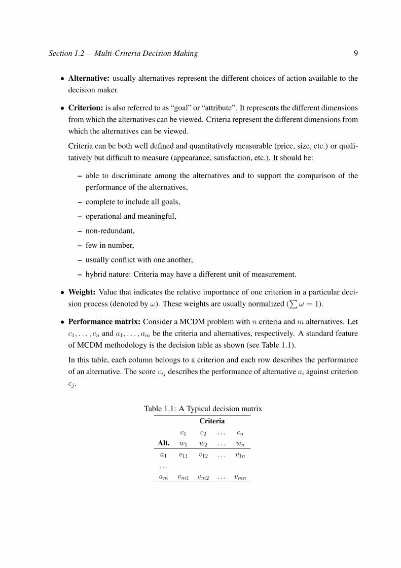
• Performance matrix: Consider a MCDM problem with n criteria and m alternatives. Letc1, . . . , cn and a1, . . . , am be the criteria and alternatives, respectively. A standard featureof MCDM methodology is the decision table as shown (see Table 1.1).
In this table, each column belongs to a criterion and each row describes the performanceof an alternative. The score vij describes the performance of alternative ai against criterioncj .
Table 1.1: A Typical decision matrixCriteria
c1 c2 . . . cn
Alt. w1 w2 . . . wn
a1 v11 v12 . . . v1n
. . .am vm1 vm2 . . . vmn
Section 1.2 – Multi-Criteria Decision Making 10
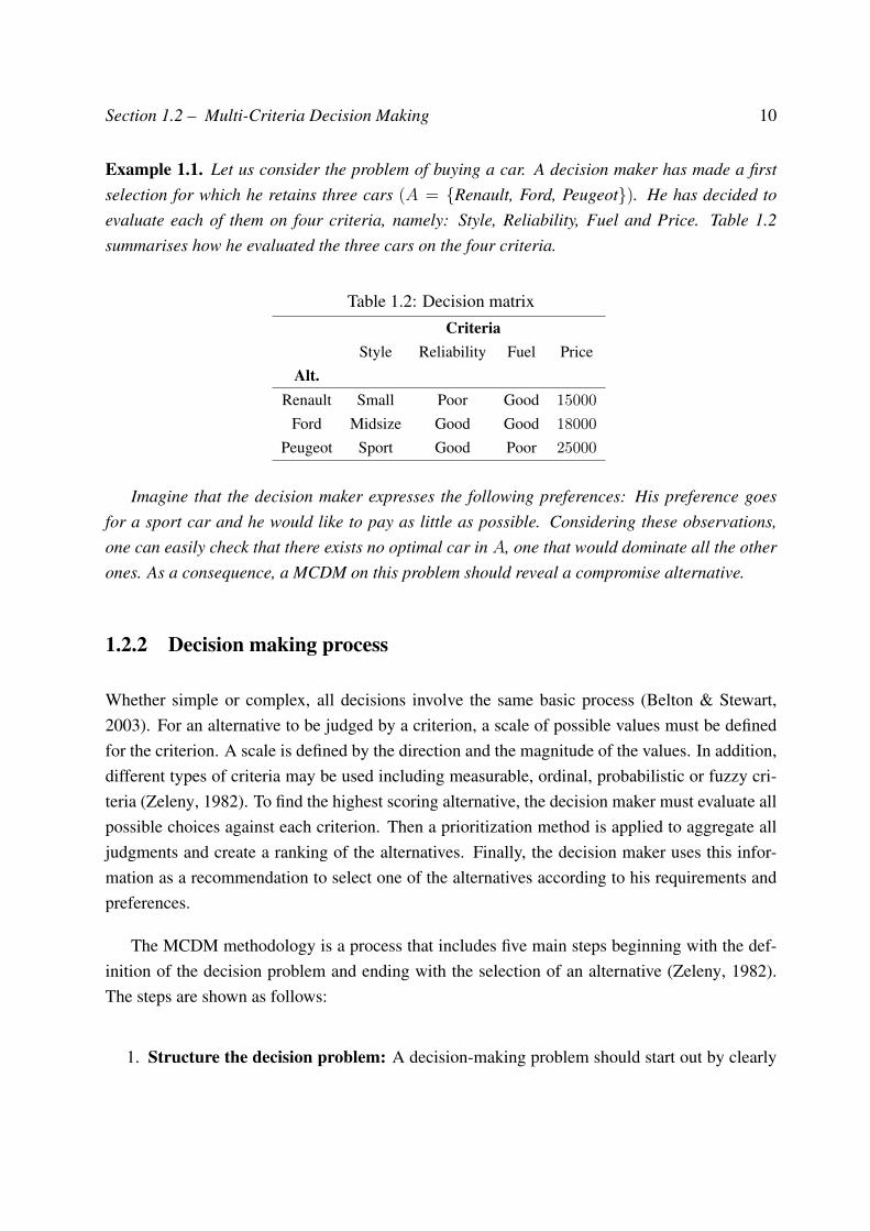
Example 1.1. Let us consider the problem of buying a car. A decision maker has made a firstselection for which he retains three cars (A = Renault, Ford, Peugeot). He has decided toevaluate each of them on four criteria, namely: Style, Reliability, Fuel and Price. Table 1.2summarises how he evaluated the three cars on the four criteria.
Table 1.2: Decision matrixCriteria
Style Reliability Fuel PriceAlt.
Renault Small Poor Good 15000
Ford Midsize Good Good 18000
Peugeot Sport Good Poor 25000
Imagine that the decision maker expresses the following preferences: His preference goesfor a sport car and he would like to pay as little as possible. Considering these observations,one can easily check that there exists no optimal car in A, one that would dominate all the otherones. As a consequence, a MCDM on this problem should reveal a compromise alternative.
1.2.2 Decision making process
Whether simple or complex, all decisions involve the same basic process (Belton & Stewart,2003). For an alternative to be judged by a criterion, a scale of possible values must be definedfor the criterion. A scale is defined by the direction and the magnitude of the values. In addition,different types of criteria may be used including measurable, ordinal, probabilistic or fuzzy cri-teria (Zeleny, 1982). To find the highest scoring alternative, the decision maker must evaluate allpossible choices against each criterion. Then a prioritization method is applied to aggregate alljudgments and create a ranking of the alternatives. Finally, the decision maker uses this infor-mation as a recommendation to select one of the alternatives according to his requirements andpreferences.
The MCDM methodology is a process that includes five main steps beginning with the def-inition of the decision problem and ending with the selection of an alternative (Zeleny, 1982).The steps are shown as follows:
1. Structure the decision problem: A decision-making problem should start out by clearly
Section 1.2 – Multi-Criteria Decision Making 11
defining the problem, discerning the alternatives, identifying the actors, the objectives andany points in conflict, together with the constraints, the degree of uncertainty and the keyissues. Even if it can be sometimes a long iterative process to come to such an agreement,it is a crucial and necessary point before proceeding to the next step.
2. Establish alternatives: Alternative identification means finding suitable alternatives to bemodeled, evaluated and analyzed.
3. Define criteria: The criteria and the way to measure the alternatives for each criterion aredefined. A weight for each criterion to reflect their relative importance to the decision isassigned.
4. Select a decision making tool: The selection of an appropriate tool is not an easy taskand depends on the concrete decision problem, as well as on the objectives of the decisionmakers. Each alternative is judged against each criterion and the selected decision makingtool can be applied to rank the alternatives or to choose a subset of the most promisingalternatives.
5. Recommendations: recommendations are given to the decision maker based on the resultsfrom the previous step. The decision maker selects one of the alternatives.
Example 1.2. In the next Figure 1.1, we see an example of the presented steps. First, the problemof choosing a car is defined. The main goal of this step is to analyze the problem: finding thereal necessities of a car, discarding other types of vehicles, making a preliminary list of possiblemodels and so on. The second step and after the initial analysis of the problem, three particularcars have been selected as the possible solution alternatives. On the third step, the evaluationcriteria have been identified. Finally, on the last step, the decision process has been carried outand the best alternative has been selected.
There exist several prioritization methods that aggregate the preferences in Step 4 and dif-ferent methods may yield different results. Although studies have been carried out to comparedifferent methods and to provide a framework for selecting the most appropriate one dependingon the problem.

Section 1.3 – Classification of MCDM methods 12
Figure 1.1: Decision making steps
1.3 Classification of MCDM methods
A wide collection of approaches is available to support individuals or groups in decision makingbut none outperforms all other methods. The selection of an appropriate method depends on theenvironment and is influenced by several factors such as available information, desired types ofoutcome or number of alternatives. In order to provide an overview of available MCDM methods,it is helpful to classify these methods.
Hajkowicz et al. (2000) classify MCDM methods under two major groupings namely contin-uous and discrete methods, based on the nature of the alternatives to be evaluated. Continuousmethods aim to identify an optimal quantity, which can vary infinitely in a decision problem.Techniques such as linear programming, goal programming and aspiration-based models areconsidered continuous. Discrete MCDM methods can be defined as decision support techniquesthat have a finite number of alternatives, a set of objectives and criteria by which the alterna-tives are to be judged and a method of ranking alternatives, based on how well they satisfy theobjectives and criteria. Discrete methods can be further subdivided into weighting methods andranking methods. These categories can be further subdivided into qualitative, quantitative andmixed methods. Qualitative methods use only ordinal performance measures. Mixed qualita-tive and quantitative methods apply different decision rules based on the type of data available.
Section 1.3 – Classification of MCDM methods 13
Quantitative methods require all data to be expressed in cardinal or ratio measurements. Ourfocus will be on the problems with a finite number of alternatives.
Value and utility-based approaches (Figueira et al., 2005; Triantaphyllou, 2000) use mathe-matical functions to assist decision makers to construct their preferences. Multi-Attribute ValueTheory (MAVT), Multi-Attribute Utility Theory (MAUT) and the Analytic Hierarchy Process(AHP) are the most common approaches within this school. The Analytic Hierarchy Process(AHP), developed by Saaty (1977, 1980), uses the same paradigm as MAVT. However, the AHPis based on a different approach to estimate relative values of criteria (weights) and score alter-natives over these criteria. The AHP is the source of several other variants, such as the geometricmean approach.
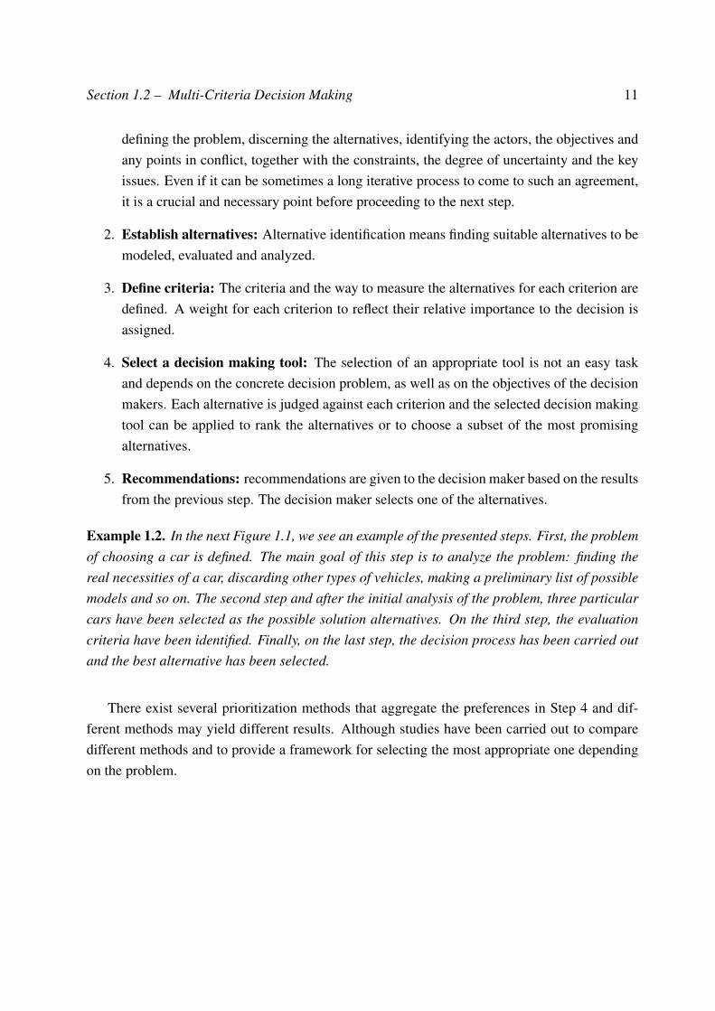
The French school uses outranking techniques such as ELECTRE (ELimination Et ChoixTraduisant la REalite) (Roy, 1968, 1990) and PROMETHEE (Preference Ranking OrganizationMETHod for Enrichment and Evaluation) (Vincke & Brans, 1985), which are based on the so-called partial comparability axiom (in contrast to the utility paradigm). Figure 1.2 presents themain MCDM families.
Figure 1.2: The main MCDM families
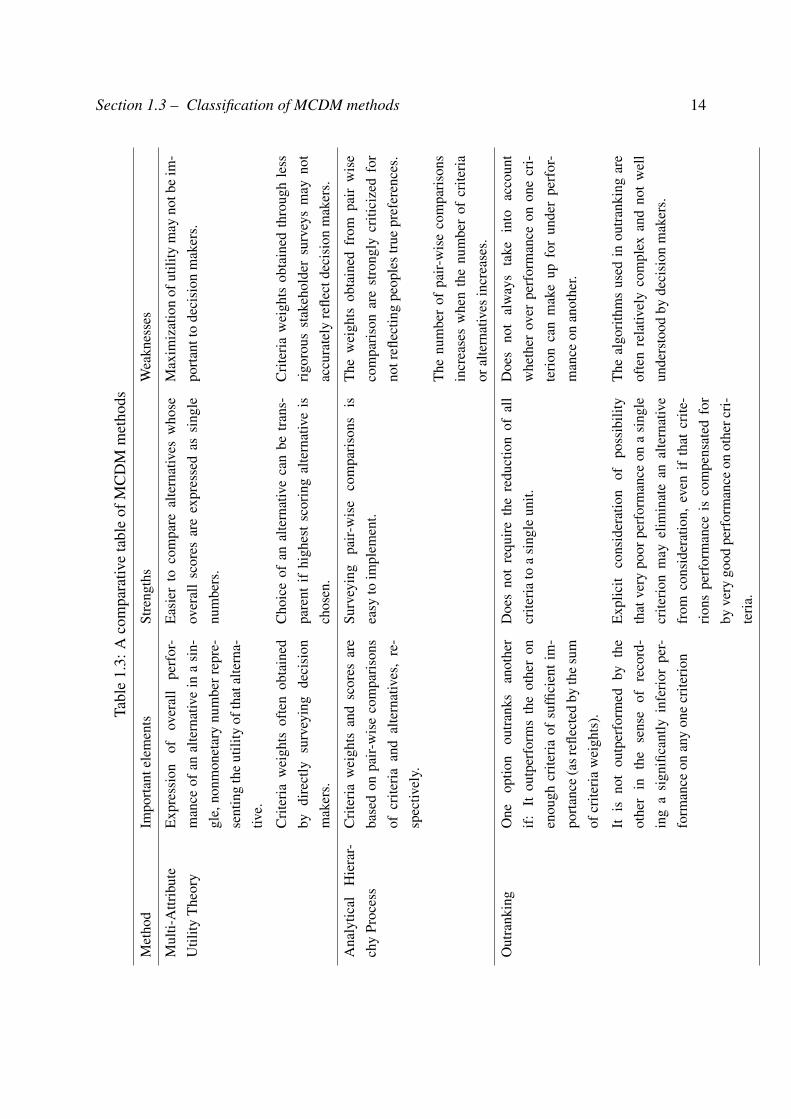
The choice of MCDM method depends not only on the criteria and the preferences of thedecision maker, but also on the type of the problem. Hence, for all the methods applied, theanalyst as well as the decision maker should acknowledge the prerequisites for its use, as wellas the advantages and drawbacks the method has. Table 1.3 defines a comparative study of themain introduced approaches: AHP, multi-attribute utility theory and outranking methods.
Section 1.3 – Classification of MCDM methods 14Ta
ble
1.3:
Aco
mpa
rativ
eta
ble
ofM
CD
Mm
etho
ds
Met
hod
Impo
rtan
tele
men
tsSt
reng
ths
Wea
knes
ses
Mul
ti-A
ttrib
ute
Util
ityT
heor
yE
xpre
ssio
nof
over
all
perf
or-
man
ceof
anal
tern
ativ
ein
asi
n-gl
e,no
nmon
etar
ynu
mbe
rrep
re-
sent
ing
the
utili
tyof
that
alte
rna-
tive.
Eas
ier
toco
mpa
real
tern
ativ
esw
hose
over
all
scor
esar
eex
pres
sed
assi
ngle
num
bers
.
Max
imiz
atio
nof
utili
tym
ayno
tbe
im-
port
antt
ode
cisi
onm
aker
s.
Cri
teri
aw
eigh
tsof
ten
obta
ined
bydi
rect
lysu
rvey
ing
deci
sion
mak
ers.
Cho
ice
ofan
alte
rnat
ive
can
betr
ans-
pare
ntif
high
est
scor
ing
alte
rnat
ive
isch
osen
.
Cri
teri
aw
eigh
tsob
tain
edth
roug
hle
ssri
goro
usst
akeh
olde
rsu
rvey
sm
ayno
tac
cura
tely
refle
ctde
cisi
onm
aker
s.
Ana
lytic
alH
iera
r-ch
yPr
oces
sC
rite
ria
wei
ghts
and
scor
esar
eba
sed
onpa
ir-w
ise
com
pari
sons
ofcr
iteri
aan
dal
tern
ativ
es,
re-
spec
tivel
y.
Surv
eyin
gpa
ir-w
ise
com
pari
sons
isea
syto
impl
emen
t.T
hew
eigh
tsob
tain
edfr
ompa
irw
ise
com
pari
son
are
stro
ngly
criti
cize
dfo
rno
trefl
ectin
gpe
ople
str
uepr
efer
ence
s.
The
num
ber
ofpa
ir-w
ise
com
pari
sons
incr
ease
sw
hen
the
num
ber
ofcr
iteri
aor
alte
rnat
ives
incr
ease
s.
Out
rank
ing
One
optio
nou
tran
ksan
othe
rif
:It
outp
erfo
rms
the
othe
ron
enou
ghcr
iteri
aof
suffi
cien
tim
-po
rtan
ce(a
srefl
ecte
dby
the
sum
ofcr
iteri
aw
eigh
ts).
Doe
sno
tre
quir
eth
ere
duct
ion
ofal
lcr
iteri
ato
asi
ngle
unit.
Doe
sno
tal
way
sta
kein
toac
coun
tw
heth
erov
erpe
rfor
man
ceon
one
cri-
teri
onca
nm
ake
upfo
run
der
perf
or-
man
ceon
anot
her.
Itis
not
outp
erfo
rmed
byth
eot
her
inth
ese
nse
ofre
cord
-in
ga
sign
ifica
ntly
infe
rior
per-
form
ance
onan
yon
ecr
iteri
on
Exp
licit
cons
ider
atio
nof
poss
ibili
tyth
atve
rypo
orpe
rfor
man
ceon
asi
ngle
crite
rion
may
elim
inat
ean
alte
rnat
ive
from
cons
ider
atio
n,ev
enif
that
crite
-ri
ons
perf
orm
ance
isco
mpe
nsat
edfo
rby
very
good
perf
orm
ance
onot
herc
ri-
teri
a.
The
algo
rith
ms
used
inou
tran
king
are
ofte
nre
lativ
ely
com
plex
and
not
wel
lun
ders
tood
byde
cisi
onm
aker
s.
Section 1.4 – Analytic Hierarchy Process as a MCDM method 15
From Table 1.3, there are many MDCM methods available in the literature. All these decisionmethodologies are differentiated by the way the objective and alternative weights are determined.In this work, we will discuss a widely used MCDM technique: the AHP approach, which is themain focus of our work.
1.4 Analytic Hierarchy Process as a MCDM method
The Analytic Hierarchy Process has been developed by Saaty (1977, 1980) and is one of thewell-known and most widely used MCDM approaches.
The AHP has attracted the interest of many researchers because it provides a flexible and eas-ily understood way to analyze and decompose the complex decision problem through breakingit into smaller and smaller parts. In addition, it is a MCDM methodology that allows subjectiveas well as objective factors to be considered in the evaluation process. The pertinent data arethen derived by using a set of pair-wise comparisons. These comparisons are used to obtainthe weights of importance of the decision criteria and the relative performance measures of thealternatives in terms of each individual decision criterion.
Indeed, that is the reason why AHP has successfully been applied to many practical problems(Saaty, 1990): from the simple problem of buying a car to the complex problems of economicplanning, supplier selection (Kahraman et al., 2003), resource allocation (Chamodrakas et al.,2010), etc.
The AHP, as a compensatory method, assumes complete aggregation among criteria anddevelops a linear additive model. The weights and scores are achieved basically by pair-wisecomparisons between all alternatives and criteria. The basic procedure to carry out the AHPmethodology will be presented in the following subsections.
1.4.1 AHP hierarchy
Constructing the hierarchical structure is the most important step in AHP method. This stepis based on findings indicating that when elaborating information, the human mind recognizesobjects and concepts, and identifies relations existing between them. Because the human mindis not able to perceive simultaneously all factors affected by an action and their connections, it

Section 1.4 – Analytic Hierarchy Process as a MCDM method 16
helps to break down complex systems into simple structures: this simplification is possible bymeans of a logical process which aims at the construction of suitable hierarchies. Therefore, thepurpose of constructing the hierarchy is to evaluate the influence of the criteria on the alternativesto attain objectives.
The number of levels depends upon the complexity of the problem and the degree of detail inthe problem. So, an AHP hierarchy has at least three levels: the main objective of the problem isrepresented at the top level of the hierarchy. Then, each level of the hierarchy contains criteria orsub-criteria that influence the decision. The last level of the structure contains the alternatives.
1.4.2 Pair-wise comparison
In AHP, once the hierarchy has been constructed, the decision maker starts with the prioritizationprocedure to determine the relative importance of the elements on each level of the hierarchy(criteria and alternatives). Elements of a problem on each level are paired (with respect to theircommon relative impacts on a property or criteria) and then compared.
To compare elements on each level of the hierarchy, AHP uses a quantitative comparisonmethod that is based on pair-wise comparisons of the following type “How important is criterionci relative to criterion cj ?”. Questions of this type are used to establish the weights for criteriaand similar questions are used to assess the performance scores for alternatives on the subjective(judgmental) criteria. “How important is alternative ai when compared to alternative ak withrespect to a specific criterion cj (in the level immediately higher)?”.
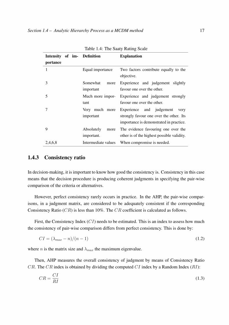
The responses to the pair-wise comparison question use the following nine-point scale (Saatyscale). Table 1.4 expresses the intensity of preference for one element versus another.
In order to compute the weights for the different criteria, for example the AHP starts creatinga pair-wise comparison matrixM (n×nmatrix). Let cij denote the value obtained by comparingcriterion ci relative to criterion cj . Of course, we set cii = 1. Furthermore, if we set cij = k, thenwe set cji = 1
k. For example, if criterion ci is absolutely more important than criterion cj and is
rated at 9, then cj must be absolutely less important than ci and is valued at 19. The entries satisfy
the following constraint:
cij.cji = 1 (1.1)
Next, the comparison matrix is formed by repeating the process for each criterion.
Section 1.4 – Analytic Hierarchy Process as a MCDM method 17
Table 1.4: The Saaty Rating Scale
Intensity of im-portance
Definition Explanation
1 Equal importance Two factors contribute equally to theobjective.
3 Somewhat moreimportant
Experience and judgement slightlyfavour one over the other.
5 Much more impor-tant
Experience and judgement stronglyfavour one over the other.
7 Very much moreimportant
Experience and judgement verystrongly favour one over the other. Itsimportance is demonstrated in practice.
9 Absolutely moreimportant.
The evidence favouring one over theother is of the highest possible validity.
2,4,6,8 Intermediate values When compromise is needed.
1.4.3 Consistency ratio
In decision-making, it is important to know how good the consistency is. Consistency in this casemeans that the decision procedure is producing coherent judgments in specifying the pair-wisecomparison of the criteria or alternatives.
However, perfect consistency rarely occurs in practice. In the AHP, the pair-wise compar-isons, in a judgment matrix, are considered to be adequately consistent if the correspondingConsistency Ratio (CR) is less than 10%. The CR coefficient is calculated as follows.
First, the Consistency Index (CI) needs to be estimated. This is an index to assess how muchthe consistency of pair-wise comparison differs from perfect consistency. This is done by:
CI = (λmax − n)/(n− 1) (1.2)
where n is the matrix size and λmax the maximum eigenvalue.
Then, AHP measures the overall consistency of judgment by means of Consistency RatioCR. The CR index is obtained by dividing the computed CI index by a Random Index (RI):
CR =CI
RI(1.3)
Section 1.5 – Illustrative example 18
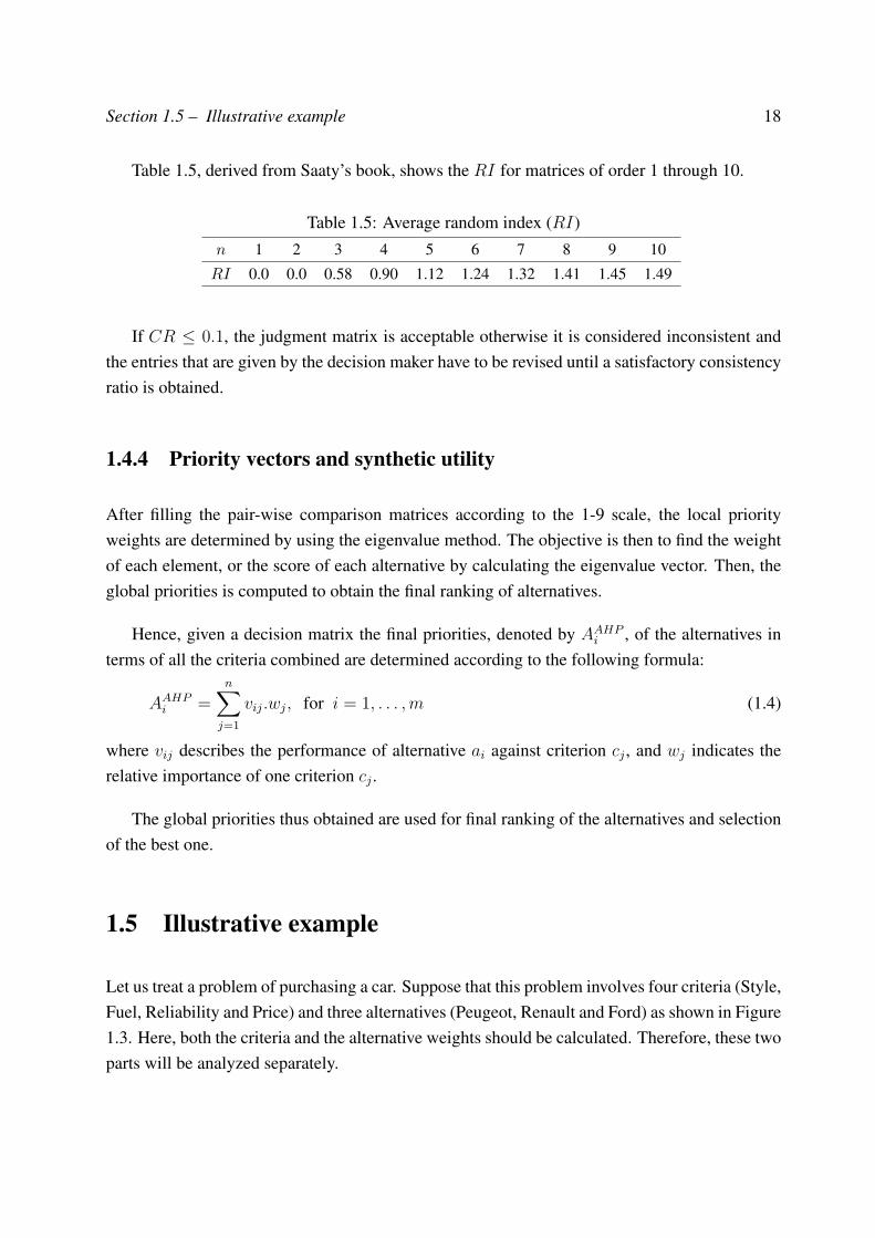
Table 1.5, derived from Saaty’s book, shows the RI for matrices of order 1 through 10.
Table 1.5: Average random index (RI)n 1 2 3 4 5 6 7 8 9 10
RI 0.0 0.0 0.58 0.90 1.12 1.24 1.32 1.41 1.45 1.49
If CR ≤ 0.1, the judgment matrix is acceptable otherwise it is considered inconsistent andthe entries that are given by the decision maker have to be revised until a satisfactory consistencyratio is obtained.
1.4.4 Priority vectors and synthetic utility
After filling the pair-wise comparison matrices according to the 1-9 scale, the local priorityweights are determined by using the eigenvalue method. The objective is then to find the weightof each element, or the score of each alternative by calculating the eigenvalue vector. Then, theglobal priorities is computed to obtain the final ranking of alternatives.
Hence, given a decision matrix the final priorities, denoted by AAHPi , of the alternatives interms of all the criteria combined are determined according to the following formula:
AAHPi =n∑j=1
vij.wj, for i = 1, . . . ,m (1.4)
where vij describes the performance of alternative ai against criterion cj , and wj indicates therelative importance of one criterion cj .
The global priorities thus obtained are used for final ranking of the alternatives and selectionof the best one.
1.5 Illustrative example
Let us treat a problem of purchasing a car. Suppose that this problem involves four criteria (Style,Fuel, Reliability and Price) and three alternatives (Peugeot, Renault and Ford) as shown in Figure1.3. Here, both the criteria and the alternative weights should be calculated. Therefore, these twoparts will be analyzed separately.
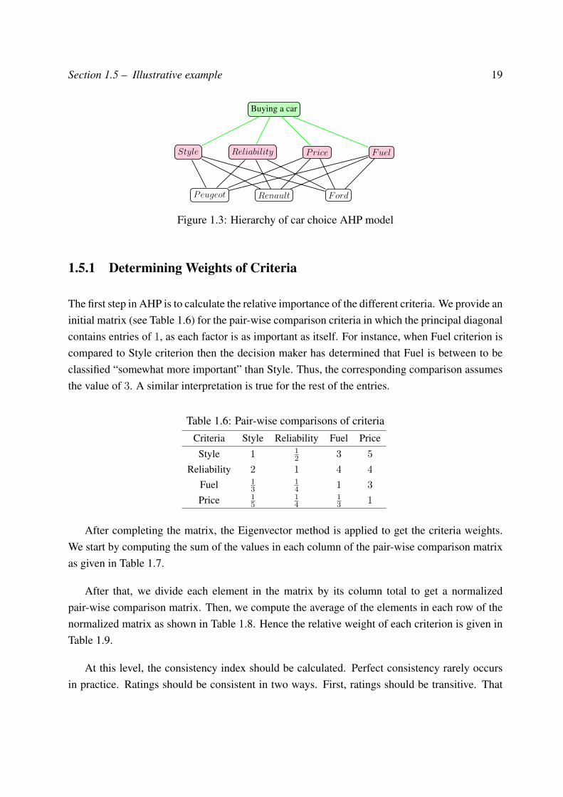
Section 1.5 – Illustrative example 19
Buying a car
Style Reliability
Peugeot Renault Ford
Price Fuel
Figure 1.3: Hierarchy of car choice AHP model
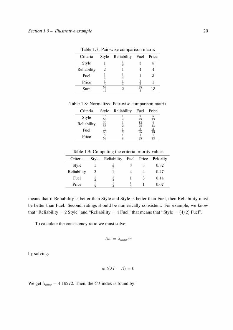
1.5.1 Determining Weights of Criteria
The first step in AHP is to calculate the relative importance of the different criteria. We provide aninitial matrix (see Table 1.6) for the pair-wise comparison criteria in which the principal diagonalcontains entries of 1, as each factor is as important as itself. For instance, when Fuel criterion iscompared to Style criterion then the decision maker has determined that Fuel is between to beclassified “somewhat more important” than Style. Thus, the corresponding comparison assumesthe value of 3. A similar interpretation is true for the rest of the entries.
Table 1.6: Pair-wise comparisons of criteriaCriteria Style Reliability Fuel Price
Style 1 12 3 5
Reliability 2 1 4 4
Fuel 13
14 1 3
Price 15
14
13 1
After completing the matrix, the Eigenvector method is applied to get the criteria weights.We start by computing the sum of the values in each column of the pair-wise comparison matrixas given in Table 1.7.
After that, we divide each element in the matrix by its column total to get a normalizedpair-wise comparison matrix. Then, we compute the average of the elements in each row of thenormalized matrix as shown in Table 1.8. Hence the relative weight of each criterion is given inTable 1.9.
At this level, the consistency index should be calculated. Perfect consistency rarely occursin practice. Ratings should be consistent in two ways. First, ratings should be transitive. That
Section 1.5 – Illustrative example 20
Table 1.7: Pair-wise comparison matrixCriteria Style Reliability Fuel Price
Style 1 12 3 5
Reliability 2 1 4 4
Fuel 13
14 1 3
Price 15
14
13 1
Sum 5315 2 25
3 13
Table 1.8: Normalized Pair-wise comparison matrixCriteria Style Reliability Fuel Price
Style 1553
14
925
513
Reliability 3053
12
1225
413
Fuel 553
18
325
313
Price 353
18
125
113
Table 1.9: Computing the criteria priority valuesCriteria Style Reliability Fuel Price PriorityStyle 1 1
2 3 5 0.32
Reliability 2 1 4 4 0.47
Fuel 13
14 1 3 0.14
Price 15
14
13 1 0.07
means that if Reliability is better than Style and Style is better than Fuel, then Reliability mustbe better than Fuel. Second, ratings should be numerically consistent. For example, we knowthat “Reliability = 2 Style” and “Reliability = 4 Fuel” that means that “Style = (4/2) Fuel”.
To calculate the consistency ratio we must solve:
Aw = λmax.w
by solving:
det(λI − A) = 0
We get λmax = 4.16272. Then, the CI index is found by:
Section 1.5 – Illustrative example 21
CI = (λmax − n)/(n− 1) = 0.0542
The final step is to calculate the CR by using the table derived from Saaty’s book (see Table 1.5):
CR = CI/RI = 0.0542/0.90 = 0.0602
where RI = 0.90 because the pair-wise comparison matrix is a matrix of order 4.
CR value is less than 0.1, so the evaluations are consistent. A similar procedure is repeatedfor the rest of matrix.
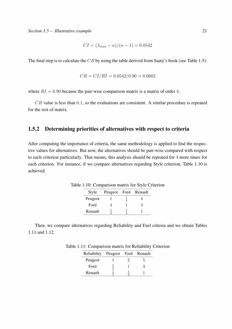
1.5.2 Determining priorities of alternatives with respect to criteria
After computing the importance of criteria, the same methodology is applied to find the respec-tive values for alternatives. But now, the alternatives should be pair-wise compared with respectto each criterion particularly. That means, this analysis should be repeated for 4 more times foreach criterion. For instance, if we compare alternatives regarding Style criterion, Table 1.10 isachieved.
Table 1.10: Comparison matrix for Style CriterionStyle Peugeot Ford Renault
Peugeot 1 14 4
Ford 4 1 4
Renault 14
14 1
Then, we compare alternatives regarding Reliability and Fuel criteria and we obtain Tables1.11 and 1.12.
Table 1.11: Comparison matrix for Reliability CriterionReliability Peugeot Ford Renault
Peugeot 1 2 5
Ford 12 1 3
Renault 15
13 1
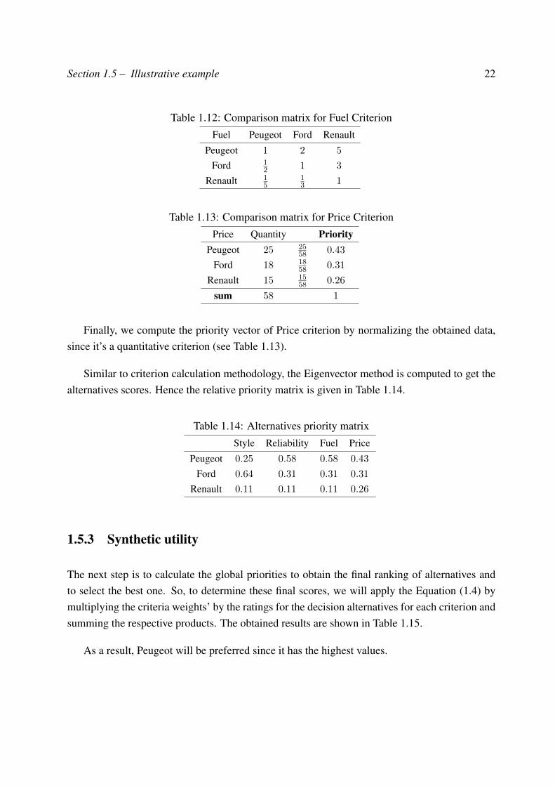
Section 1.5 – Illustrative example 22
Table 1.12: Comparison matrix for Fuel CriterionFuel Peugeot Ford Renault
Peugeot 1 2 5
Ford 12 1 3
Renault 15
13 1
Table 1.13: Comparison matrix for Price CriterionPrice Quantity Priority
Peugeot 25 2558 0.43
Ford 18 1858 0.31
Renault 15 1558 0.26
sum 58 1
Finally, we compute the priority vector of Price criterion by normalizing the obtained data,since it’s a quantitative criterion (see Table 1.13).
Similar to criterion calculation methodology, the Eigenvector method is computed to get thealternatives scores. Hence the relative priority matrix is given in Table 1.14.
Table 1.14: Alternatives priority matrixStyle Reliability Fuel Price
Peugeot 0.25 0.58 0.58 0.43
Ford 0.64 0.31 0.31 0.31
Renault 0.11 0.11 0.11 0.26
1.5.3 Synthetic utility
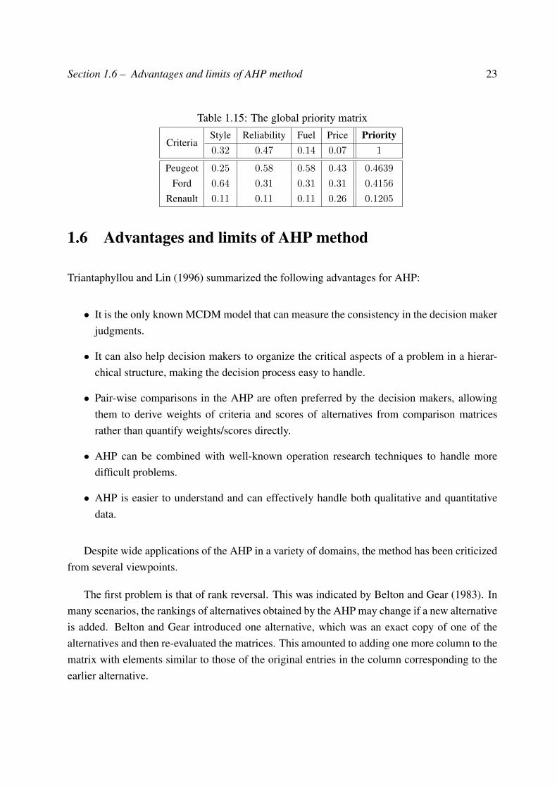
The next step is to calculate the global priorities to obtain the final ranking of alternatives andto select the best one. So, to determine these final scores, we will apply the Equation (1.4) bymultiplying the criteria weights’ by the ratings for the decision alternatives for each criterion andsumming the respective products. The obtained results are shown in Table 1.15.
As a result, Peugeot will be preferred since it has the highest values.
Section 1.6 – Advantages and limits of AHP method 23
Table 1.15: The global priority matrix
CriteriaStyle Reliability Fuel Price Priority0.32 0.47 0.14 0.07 1
Peugeot 0.25 0.58 0.58 0.43 0.4639
Ford 0.64 0.31 0.31 0.31 0.4156
Renault 0.11 0.11 0.11 0.26 0.1205
1.6 Advantages and limits of AHP method
Triantaphyllou and Lin (1996) summarized the following advantages for AHP:
• It is the only known MCDM model that can measure the consistency in the decision makerjudgments.
• It can also help decision makers to organize the critical aspects of a problem in a hierar-chical structure, making the decision process easy to handle.
• Pair-wise comparisons in the AHP are often preferred by the decision makers, allowingthem to derive weights of criteria and scores of alternatives from comparison matricesrather than quantify weights/scores directly.
• AHP can be combined with well-known operation research techniques to handle moredifficult problems.
• AHP is easier to understand and can effectively handle both qualitative and quantitativedata.
Despite wide applications of the AHP in a variety of domains, the method has been criticizedfrom several viewpoints.
The first problem is that of rank reversal. This was indicated by Belton and Gear (1983). Inmany scenarios, the rankings of alternatives obtained by the AHP may change if a new alternativeis added. Belton and Gear introduced one alternative, which was an exact copy of one of thealternatives and then re-evaluated the matrices. This amounted to adding one more column to thematrix with elements similar to those of the original entries in the column corresponding to theearlier alternative.
Section 1.7 – Conclusion 24
Secondly, the human preference model is uncertain and decision makers might be unable toassign exact numerical values to the comparison judgments. Although, the use of the discretescale of 1 − 9 for performing pair-wise comparative analysis has the advantage of simplicity, adecision maker may find it extremely difficult to express the strength of his preferences and toprovide exact pair-wise comparison judgments.
Also, the number of pair-wise comparisons increases when the number of criteria or alterna-tives increases.
To handle these pitfalls, many extensions of this standard AHP method have been developed.A survey of these extensions will be provided in Chapter 2.
1.7 Conclusion
In the first part of this Chapter, we have briefly presented the fundamental concepts of the MCDMmethod. We have given an overview of the available MCDM methods. In the second part, wehave presented with more details the basics of the AHP method, one of the most widely usedapproaches, with a detailed example.
Despite the advantages of AHP method, several researches are focusing on improving moreand more the results provided by this approach, especially, in an environment where uncertaintymay exist in the different levels relative to a decision making problem. Consequently, standardAHP method should be adapted to handle such imperfection. Therefore, several approachesare combined within uncertain theories such as probability theory, fuzzy set theory and belieffunction theory.
The next Chapter is devoted to the presentation of the main developed approaches, especiallythose developed under the belief function framework. This topic besides belief function theorydealing uncertainty will be at the core of some contributions of this Thesis.
Chapter 2AHP method under uncertainty
2.1 Introduction
The Analytic Hierarchy Process (AHP) has emerged as a successful and practical MulticriteriaDecision Making (MCDM) technique applied in a variety of areas. This approach gives goodresults in a context in which everything is known with certainty. However, the reality is connectedto uncertainty and imprecision by nature. Hence, one of the main problems of the standard AHPis that it does not take into account uncertainty in the judgments since the matrices of judgmentsare deterministic. In real applications, the decision maker is always subject to uncertainty whileexpressing their judgments and do not like to be forced to give deterministic answers. Moreover,by eliminating uncertainty from the judgments it becomes impossible to evaluate its impact onthe final decision’s uncertainty. This limitation greatly reduces the confidence of the users on thefinal results of the AHP technique.
To overcome these difficulties and to extend the AHP on a more real elicitation procedure,several AHP methods are combined within uncertain theories. As a result, three different familiesof approaches for the problem are proposed: the fuzzy approach, the probabilistic approach andthe belief approach.
In this Chapter, we will especially focus on both AHP method under fuzzy set theory andAHP method under the belief function framework, therefore some known fuzzy AHP will bedetailed. Regarding the belief function framework, we will present Utkin method (Utkin &
25
Section 2.2 – AHP method under uncertainty 26
Simanova, 2008) and Evidential Reasoning approach (ER-MCDM) (Dezert et al., 2010) and wewill give more details about DS/AHP (Beynon et al., 2000) which constitutes one of the mainfocus of our work.
This Chapter is organized as follows: we start, in Section 2.2, by describing the main devel-oped methods. Then, in Section 2.3, we introduce the belief functions that are used to representknowledge under the belief function framework. Several basic operations are also detailed. InSection 2.4, we present some AHP approaches under the belief function theory.
2.2 AHP method under uncertainty
Probabilistic AHP (Vargas, 1982; Escobar & Moreno-Jimenez, 2000; Manassero et al., 2004),fuzzy AHP (Laarhoven & Pedrycz, 1983; Lootsma, 1997) are compact representations of un-certainty in different levels. Their success is due to their capacity of handling imperfection andsolving more complex problems. In this Section, we briefly recall these approaches.
2.2.1 Brief refresher on Probabilistic AHP
The first work was introduced by Vargas (1982). He tries to demonstrate that if the judgments ina matrix are gamma distributed variables then the eigenvector follows a Dirichlet, or multinomialbeta, distribution. However, there are two problems with this approach. First, the judgments inthe pair-wise comparison matrix are reciprocals since the gamma distribution is not reciprocal.Therefore defining an element Vij , of the matrix as a gamma random variable, we have thatVji = 1
Vij, is not distributed as a gamma. Therefore, the order in which the decision maker
gives his judgments modifies the probability distributions of the elements of the matrix and thisgoes against one of the main principle of the AHP methodology. Secondly, the elements ofthe principal diagonal are treated as random variables but by definition they must be equal to 1(Manassero et al., 2004).
Escobar and Moreno-Jimenez (2000) have presented a method that solves both problems,demonstrating that if a judgment follows a reciprocal distribution then also its reciprocal is arandom variable that follows the same kind of distribution. Arbel (1989) proposes a hybridstochastic-interval AHP (SIAHP) approach to address uncertainty in group decision making byintegrating interval judgment. The goal of this method is to process a matrix whose entries
Section 2.2 – AHP method under uncertainty 27
are intervals. These intervals may be assumed to be constraints in an optimization problem,or intervals characterized by some type of probability distribution. The optimization approachyields a vector of intervals, one for each of the components and the simulation approach yields aprobability distribution, for the priorities.
2.2.2 Brief refresher on fuzzy AHP
Fuzzy set theory
The fuzzy set theory was introduced by Zadeh (1965). This theory, which was a generalizationof classic set theory, allowed the membership functions to operate over the range of real numbers[0, 1]. The uncertainty can be represented by the fuzzy number. A triangular fuzzy number is aspecial fuzzy set F = (x, µ(x)), x ∈ <, where x takes its values on the real line and µ(x) is acontinuous mapping from < to the closed interval [0, 1].
A triangular fuzzy number is denoted by M = (a, b, c), where a ≤ b ≤ c, can be describedas:
µM(x) =
0 , x < ax−ab−a , a ≤ x ≤ bc−xc−b , b < x ≤ c
1 , x > c
(2.1)
in which the parameters a, b and c respectively denote the smallest possible value, the mostpromising value and the largest possible value that describe a fuzzy event.
Fuzzy AHP method
Fuzzy AHP (Laarhoven & Pedrycz, 1983; Chang, 1996) uses fuzzy set theory to express the un-certain comparison judgments as a fuzzy numbers. The main steps of fuzzy AHP are as follows:
1. Structuring decision hierarchy. Similar to standard AHP, the first step is to break down thecomplex decision making problem into a hierarchical structure.
Section 2.2 – AHP method under uncertainty 28
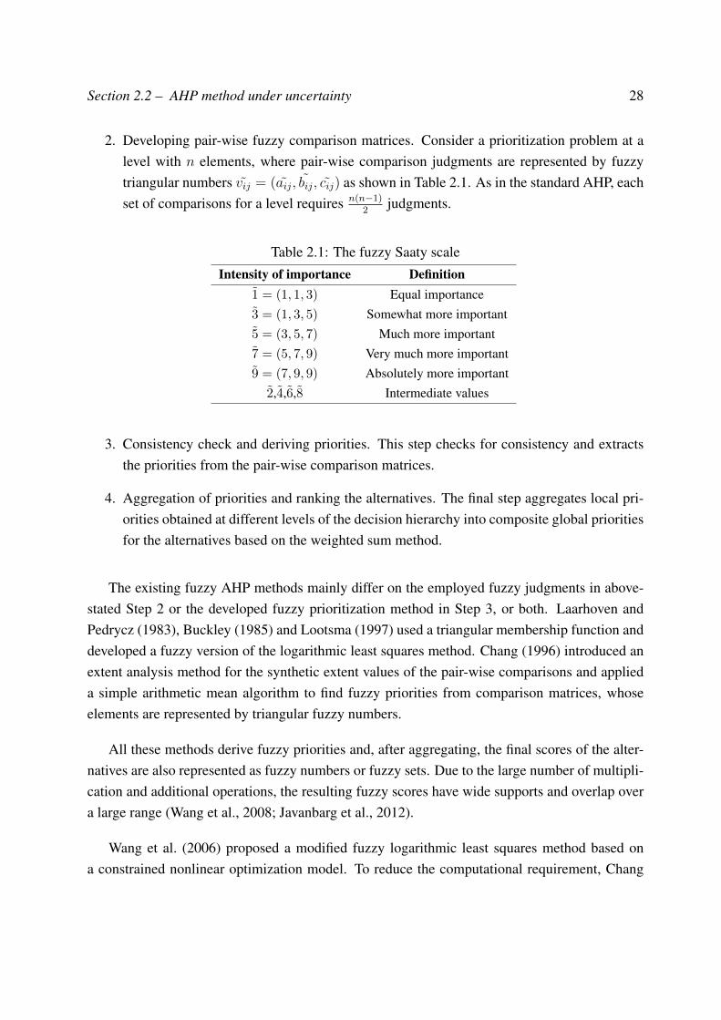
2. Developing pair-wise fuzzy comparison matrices. Consider a prioritization problem at alevel with n elements, where pair-wise comparison judgments are represented by fuzzytriangular numbers vij = (aij, bij, cij) as shown in Table 2.1. As in the standard AHP, eachset of comparisons for a level requires n(n−1)
2judgments.
Table 2.1: The fuzzy Saaty scaleIntensity of importance Definition
1 = (1, 1, 3) Equal importance3 = (1, 3, 5) Somewhat more important5 = (3, 5, 7) Much more important7 = (5, 7, 9) Very much more important9 = (7, 9, 9) Absolutely more important
2,4,6,8 Intermediate values
3. Consistency check and deriving priorities. This step checks for consistency and extractsthe priorities from the pair-wise comparison matrices.
4. Aggregation of priorities and ranking the alternatives. The final step aggregates local pri-orities obtained at different levels of the decision hierarchy into composite global prioritiesfor the alternatives based on the weighted sum method.
The existing fuzzy AHP methods mainly differ on the employed fuzzy judgments in above-stated Step 2 or the developed fuzzy prioritization method in Step 3, or both. Laarhoven andPedrycz (1983), Buckley (1985) and Lootsma (1997) used a triangular membership function anddeveloped a fuzzy version of the logarithmic least squares method. Chang (1996) introduced anextent analysis method for the synthetic extent values of the pair-wise comparisons and applieda simple arithmetic mean algorithm to find fuzzy priorities from comparison matrices, whoseelements are represented by triangular fuzzy numbers.
All these methods derive fuzzy priorities and, after aggregating, the final scores of the alter-natives are also represented as fuzzy numbers or fuzzy sets. Due to the large number of multipli-cation and additional operations, the resulting fuzzy scores have wide supports and overlap overa large range (Wang et al., 2008; Javanbarg et al., 2012).
Wang et al. (2006) proposed a modified fuzzy logarithmic least squares method based ona constrained nonlinear optimization model. To reduce the computational requirement, Chang
Section 2.2 – AHP method under uncertainty 29
(1996) proposed the extent analysis to derive the crisp weights from triangular membership func-tions and this has been applied to numerous real-life problems such as in implementing cleanerproduction in a manufacturing firm (Tseng et al., 2009) and prioritizing environmental issues inoff-shore oil and gas operations (M. Yang et al., 2011). Also, fuzzy AHP extensions have beenextensively applied to solve supplier selection problem (Junior et al., 2014).
Some drawbacks in using existing fuzzy AHP were also pointed out by Wang et al. (2006).Mikhailov (2003) argued that these fuzzy AHP variants require an additional defuzzification pro-cedure to convert fuzzy weights to crisp weights and he proposed fuzzy preference programmingtechnique to derive the crisp weights from the fuzzy pair-wise comparison judgment matrix.
Comments
Many AHP extensions have been developed and the difference between them mainly lies in thetype of uncertainty related to the problem at hand and especially in the way of dealing with thatuncertainty when making a decision. Therefore, probability and fuzzy set theories are widelyused to represent such uncertainty but they fail to handle imprecise, uncertain and conflictinginformation. For that reason, we are interested in belief function theory which offers a naturaland simple tool to handle imperfect information. It represents an appropriate framework forexperts to express their partial beliefs in a much more flexible way.
The belief function theory, known also as the theory of evidence or Dempster-Shafer theory,is a general framework for reasoning with uncertainty (Smets & Kennes, 1994). It shows itsefficiency in many real-world applications such classification (Elouedi et al., 2001; Trabelsi etal., 2011; Smets, 2001), image processing (Denoeux & Zouhal, 2001; Lefevre et al., 2000),multi-criteria decision making (Beynon et al., 2001; Frikha & Moalla, 2014; J. Yang et al.,2006), etc.
In the next Section, we will especially focus on the belief function theory and we will explainin details its different belief functions, which are used to represent knowledge. On the otherhand, we will present more the main proposed approaches under this theory.
Section 2.3 – Belief function theory 30
2.3 Belief function theory
The term Dempster-Shafer refers to the origin of the theory. In fact, in the 1960s, Dempsterdeveloped the basic ideas of a new mathematical theory of uncertainty that includes a kind ofupper and lower probabilities (Dempster, 1967, 1968). Then, in 1970s, it was extended by Shafer(1976) to what is now known as belief function theory.
Several interpretations of this theory have been proposed (Smets, 1991) among them: theDempster model (Dempster, 1967, 1968), the lower probability model (Walley, 1991), the theoryof hints (Kohlas & Monney, 1995) and the Transferable Belief Model (TBM) (Smets & Kennes,1994). In this Thesis, we deal with the interpretation of the belief function theory as explainedby the TBM.
2.3.1 Basic concepts
Let us denote by Θ the finite non empty set including n elementary events (hypotheses) repre-senting the solutions of a given problem. These events are assumed to be exhaustive and mutuallyexclusive. The set Θ, called the frame of discernment, is defined as:
Θ = θ1, θ2, . . . , θn (2.2)
All the subsets of Θ belong to the power set of Θ, denoted by 2Θ and every element of 2Θ iscalled a proposition or an event:
2Θ = A/A ⊆ Θ (2.3)
In Shafer’s model, Θ is assumed to be exhaustive (Shafer, 1976) which means that the so-lution to a given problem is unique and is necessarily included in this frame of discernment.However, in the TBM, Smets relaxed this condition, considering that it is sometimes difficult tolist a priori all the possible hypotheses related to a given problem domain. He induced what hecalled the open-world assumption and the closed-world assumption (Smets, 1990, 1998).
Under the open-world assumption, Θ is not necessarily exhaustive. It means that we admitthat the problem domain can include some unknown hypotheses that we did not mention into theframe of discernment, whereas under the closed-world assumption the frame of discernment isexhaustive.
Section 2.3 – Belief function theory 31
Example 2.1. Let us treat a problem of identification of childhood diseases. Some of the mostcommon illnesses of childhood cause skin eruptions and are known as exanthems. The child-hood exanthems include measles, rubella and fifth disease. All of these infections have the samesymptoms.
Suppose the frame of discernment Θ related to this problem is defined as follows:
Θ = measles, rubella, fifth disease
Then, the power set of Θ is:
2Θ = ∅, measles, rubella, fifth disease,measles, rubella, measles, fifth disease, rubella, fifth disease,Θ
Basic belief assignment
The basic belief assignment (bba), called initially by Shafer basic probability assignment (Shafer,1976), assigns a belief in range [0, 1] to every member of 2Θ (bba can assign belief to any propo-sition in the frame and not only to the elementary ones) such that their sum is 1. That means, afunction is called a basic belief assignment such that (Shafer, 1976):∑
A⊆Θ
m(A) = 1 (2.4)
The value m(A), named a basic belief mass (bbm), represents the portion of belief committedexactly to the event A and not for a particular subset of A. In this way, committing belief to aproposition A does not necessarily imply that the remaining belief is committed to A. The massm(Θ) quantifies the part of belief committed to the whole frame Θ. It represents the beliefs thatare not assigned to the different subsets of Θ.
The subsets of Θ such that m(A) > 0 are called focal elements and F(m) is the set of all itselements relative to the bba m. The union of all focal elements is called core.
Similarly, m(∅) represents the part of belief allocated to the empty set. Shafer has initiallyimposed the condition m(∅) = 0. This condition reflects the fact that no belief ought to beallocated to the empty set. Such bba is called a normalized basic belief assignment. However, this
Section 2.3 – Belief function theory 32
condition is relaxed in the TBM. The allocation of a positive mass to the empty set (m(∅) > 0)
is interpreted as a consequence of the open-world assumption (Smets, 1990). A mass of belief isassigned to each possible subset.
The normalization process is defined as follows:
m(A) =
0 if A = ∅K.m(A) otherwise
(2.5)
where K−1 = 1−m(∅). It is called the normalization factor.
Since the belief function theory models several types of imperfection, special bbas weredefined. In particular, we have:
• Vacuous bba: is a normalized bba with Θ is its unique focal element (Shafer, 1976). So,its corresponding bba is defined as follows:
m(Θ) = 1 and m(A) = 0, ∀A ⊂ Θ, A 6= Θ (2.6)
Such basic belief assignment quantifies the state of total ignorance, in which there is noreason to belief in any proposition more than another and all the propositions are plausible.
• Categorical bba: the case where the bba has a unique focal element A (Mellouli, 1987):
m(A) = 1, ∀A ⊂ Θ (2.7)
• Bayesian bba: is a bba where all focal elements are singletons. It is a particular case ofprobabilities.
if m(A) > 0 then |A| = 1, where |A| stands for the cardinal of A. (2.8)
• Certain bba: is a bba having only one focal element which is a singleton.
m(A) = 1, ∀A ∈ Θ (2.9)
• Consonant bba: is a bba in which all the focal elements (A1, A2, . . . , An) are nested, thatis A1 ⊆ A2 ⊆ · · · ⊆ An (Dubois et al., 2001).
Example 2.2. Let us consider the example defined in Example 2.1. Table 2.2 shows an exampleof bbas expressed on the frame of discernment Θ.
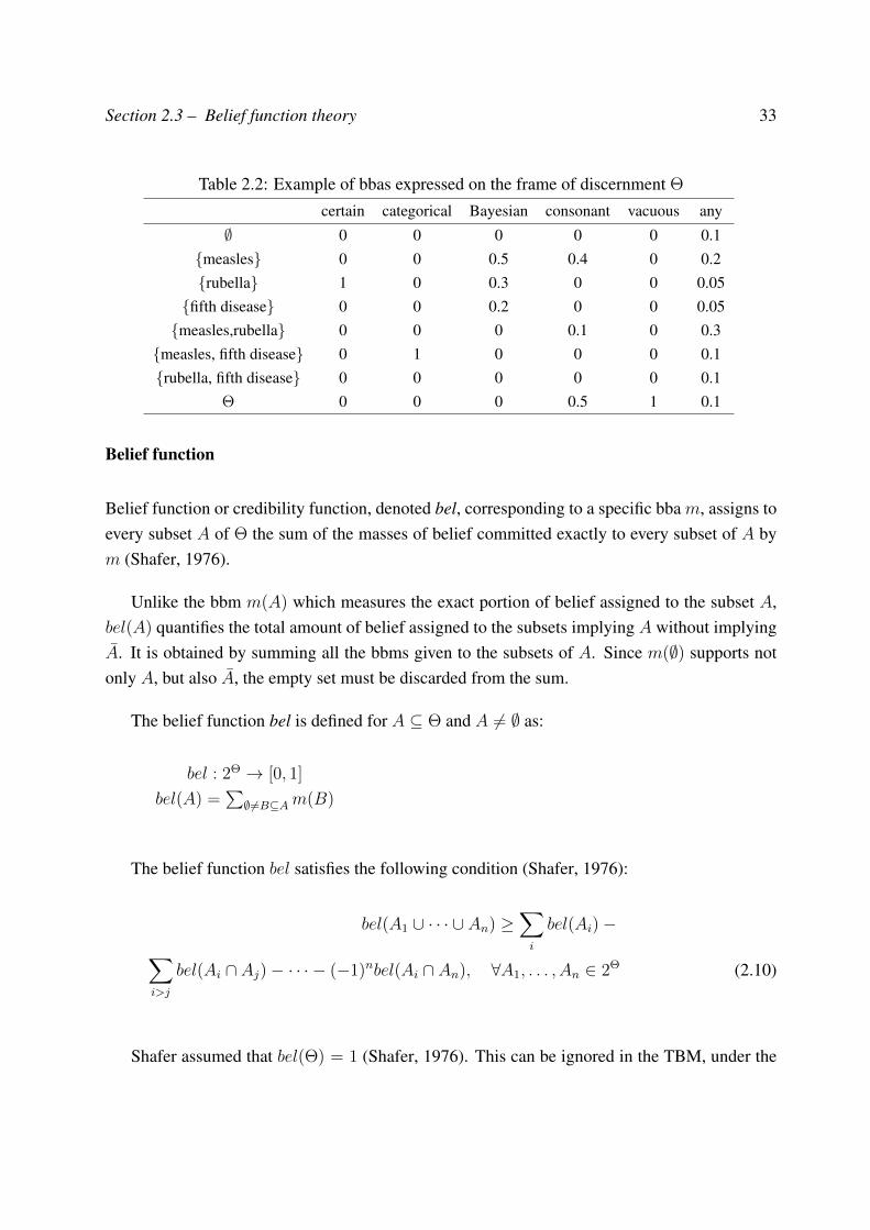
Section 2.3 – Belief function theory 33
Table 2.2: Example of bbas expressed on the frame of discernment Θ
certain categorical Bayesian consonant vacuous any
∅ 0 0 0 0 0 0.1measles 0 0 0.5 0.4 0 0.2rubella 1 0 0.3 0 0 0.05
fifth disease 0 0 0.2 0 0 0.05measles,rubella 0 0 0 0.1 0 0.3
measles, fifth disease 0 1 0 0 0 0.1rubella, fifth disease 0 0 0 0 0 0.1
Θ 0 0 0 0.5 1 0.1
Belief function
Belief function or credibility function, denoted bel, corresponding to a specific bba m, assigns toevery subset A of Θ the sum of the masses of belief committed exactly to every subset of A bym (Shafer, 1976).
Unlike the bbm m(A) which measures the exact portion of belief assigned to the subset A,bel(A) quantifies the total amount of belief assigned to the subsets implying A without implyingA. It is obtained by summing all the bbms given to the subsets of A. Since m(∅) supports notonly A, but also A, the empty set must be discarded from the sum.
The belief function bel is defined for A ⊆ Θ and A 6= ∅ as:
bel : 2Θ → [0, 1]
bel(A) =∑∅6=B⊆Am(B)
The belief function bel satisfies the following condition (Shafer, 1976):
bel(A1 ∪ · · · ∪ An) ≥∑i
bel(Ai)−∑i>j
bel(Ai ∩ Aj)− · · · − (−1)nbel(Ai ∩ An), ∀A1, . . . , An ∈ 2Θ (2.10)
Shafer assumed that bel(Θ) = 1 (Shafer, 1976). This can be ignored in the TBM, under the
Section 2.3 – Belief function theory 34
open world assumption, requiring only that bel(Θ) < 1.
Example 2.3. Let us consider the same example defined in Example 2.1. Suppose a doctorexpressing a piece of evidence concerning the diseases. The obtained bba is then defined asfollows:m(measles) = 0.6;m(measles, rubella) = 0.2;m(Θ) = 0.2.
The belief function bel corresponding to the bba m is defined by:bel(measles) = 0.6;bel(rubella) = 0;bel(fifth disease) = 0;bel(measles, rubella) = 0.8;bel(measles, fifth disease) = 0.6;bel(rubella, fifth disease) = 0;bel(Θ) = 1.
For example, 0.6 represents the part of belief exactly committed to the hypothesis “the patienthas measles”.
Plausibility function
The plausibility function pl, expresses the maximum amount of specific support that could begiven to a proposition A in Θ. It measures the degree of belief committed to the propositionscompatible with A. pl(A) is then obtained by summing the bbms given to the subsets B suchthat B ∩ A 6= ∅ (Shafer, 1976).
The plausibility function is defined by:
pl : 2Θ → [0, 1]
pl(A) =∑
B∩A6=∅m(B)
There is a simple relationship between the belief function bel and the plausibility function plassociated with a mass function m:
pl(A) = bel(Θ)− bel(A) ∀A ⊆ Θ (2.11)
Section 2.3 – Belief function theory 35
where A denotes the complement of A.
Also,
pl(A) = bel(Θ)− bel(A) ∀A ⊆ Θ (2.12)
Example 2.4. Let us continue with Example 2.1. The plausibility function pl corresponding tothe bba m is defined by:pl(measles) = 1;pl(rubella) = 0.4;pl(fifth disease) = 0.2;pl(measles, rubella) = 1;pl(measles, fifth disease) = 1;pl(rubella, fifth disease) = 0.4;pl(Θ) = 1.
For example, 0.4 represents the maximum degree of belief that could be given to the proposi-tion “rubella”.
2.3.2 Basic tools
Combination rules
Let m1 and m2 be two bbas induced from two distinct information sources and defined on thesame frame of discernment Θ. The combination of these bbas induces a bba on the same frameΘ and it can be either conjunctive or disjunctive.
The choice of one of these rules of combination for aggregating pieces of evidence may beguided by meta-belief concerning the reliability of the sources. In fact, if we know that bothsources of information are fully reliable, then we combine them conjunctively. However, if weknow that at least one of the two sources is reliable, then we combine them disjunctively (Smets,1990, 1991).
1. Conjunctive rule of combination: When we know that both sources of information arefully reliable, the resulting bba is computed by the conjunctive rule of combination. Hence,
Section 2.3 – Belief function theory 36
the induced bba quantifies the combined impact of the two pieces of evidence. It is definedas follows (Smets, 1990):
(m1 ∩©m2)(A) =∑
B,C⊆Θ,B∩C=A
m1(B)m2(C), ∀A ⊆ Θ (2.13)
The conjunctive rule is considered as the unnormalized Demspter rule of combinationdealing with the closed world assumptions, defined as follows (Shafer, 1986):
(m1 ⊕m2)(A) = K.∑
B,C⊆Θ,B∩C=A
m1(B)m2(C) (2.14)
where
K−1 = 1−∑
B,C⊆Θ,B∩C=∅
m1(B)m2(C) (2.15)
and
(m1 ⊕m2)(∅) = 0 (2.16)
K is called the normalization factor.
The conjunctive rule of combination is characterized by the following properties:
• Commutativity:
m1 ∩©m2 = m2 ∩©m1 (2.17)
• Associativity:
(m1 ∩©m2) ∩©m3 = m1 ∩©(m2 ∩©m3) (2.18)
• Non-idempotency:
m ∩©m 6= m (2.19)
• Neutral element:The neutral element within the conjunctive rule of combination is the vacuous basicbelief assignment representing the total ignorance:
m ∩©m0 = m (2.20)
where m0 is a vacuous bba.
Section 2.3 – Belief function theory 37
2. Disjunctive rule of combination: The dual of the conjunctive rule is the disjunctive rule ofcombination. We use it when we only know that at least one of the sources of informationis reliable but we do not know which one is reliable (Smets, 1998). It is defined as:
(m1 ∪©m2)(A) =∑
B,C⊆Θ,B∪C=A
m1(B)m2(C) (2.21)
The disjunctive rule of combination (as the conjunctive rule of combination) is commuta-tive and associative.
3. In addition to the conjunctive and disjunctive combination rule, a larger choice of combi-nation rules has been recognized by many researchers involved in real-world applications(Lefevre et al., 2002; Yager, 1987): Yager’s rule (Yager, 1987), the cautious rule (Denoeux,2006), Inagaki’s unified combination rule (Inagaki, 1991) and combination with adaptedconflict (Lefevre & Elouedi, 2013), etc.
Example 2.5. Let us consider two distinct doctors’ evidences S1 and S2. The first evidence isexpressed by a bba m1 and defined as follows:m1(measles) = 0.4;m1(rubella) = 0.1;m1(measles, fifth disease) = 0.3;m1(Θ) = 0.2;
The second evidence is expressed by m2 defined as follows:m2(fifth disease) = 0.5;m2(measles, fifth disease) = 0.4;m2(Θ) = 0.1;
The bba corresponding to the conjunctive combination of both pieces of evidence is definedas follows:(m1 ∩©m2)(∅) = 0.2 + 0.05 + 0.04 = 0.29;(m1 ∩©m2)(measles) = 0.16 + 0.04 = 0.2;(m1 ∩©m2)(rubella) = 0.01;(m1 ∩©m2)(fifth disease) = 0.1 + 0.15 = 0.25;(m1 ∩©m2)(measles, fifth disease) = 0.08 + 0.12 + 0.02 = 0.22;(m1 ∩©m2)(Θ) = 0.03;
m1 ∩©m2 represents the joint bba induced from the combination of m1 and m2 by using theconjunctive rule of combination.
Section 2.3 – Belief function theory 38
Once the disjunctive rule of combination is applied, we get:(m1 ∪©m2)(measles, fifth disease) = 0.2 + 0.1 + 0.16 + 0.08 = 0.54;(m1 ∪©m2)(rubella, fifth disease) = 0.05;(m1 ∪©m2)(Θ) = 0.15 + 0.12 + 0.04 + 0.02 + 0.03 + 0.04 + 0.01 = 0.41;
m1 ∪©m2 represents the joint bba induced from the combination of m1 and m2 by using thedisjunctive rule of combination.
Discounting
In the Transferable Belief Model, discounting allows to take in consideration the reliability ofthe information source that generates the bba m.
For α ∈ [0,1], let (1-α) be the degree of confidence (“reliability”) that we assign to the sourceof information. It quantifies the strength of reliability given to the expert (Smets, 1992).
If the source is not fully reliable, the expert’s opinions are represented as follows:
mα(A) = (1− α)m(A), ∀A ⊂ Θ (2.22)
mα(Θ) = α + (1− α)m(Θ) (2.23)
where α is the discounting factor.
Example 2.6. The degree of reliability given to the expert is equal to 0.7. If we consider this bbadefined as follows:m(measles) = 0.4;m(measles,fifth disease) = 0.3;m(Θ) = 0.3;
So, we obtain after discounting this bba:mα(measles) = 0.4× 0.7 = 0.28;mα(measles,fifth disease) = 0.3× 0.7 = 0.21;mα(Θ) = 0.3 + (0.3× 0.7) = 0.51;
Section 2.3 – Belief function theory 39
2.3.3 Decision making
It is necessary, when making a decision, to select the most likely hypothesis. Some solutions aredeveloped to ensure the decision making within the belief function theory. One of the most usedis the pignistic probability proposed within the TBM (Smets & Kennes, 1994).
The TBM is a model that aims at quantifying someone’s degree of belief. It is based on twolevels (Smets & Kennes, 1994):
• The credal level where beliefs are entertained and represented by belief functions.
• The pignistic level where beliefs are used to make decisions and represented by probabilityfunctions called the pignistic probabilities.
When a decision must be made, beliefs held at the credal level induce a probability measure atthe pignistic measure denoted BetP (Smets, 1998):
BetP (A) =∑B⊆Θ
|A ∩B||B|
m(B)
(1−m(∅)), ∀A ∈ Θ (2.24)
It includes normalization and division of bbas assigned to focal elements by their cardinality.
Example 2.7. Assume that at the credal level, beliefs are represented by the following bba:m(measles) = 0.7;m(measles,rubella) = 0.2;m(Θ) = 0.1;
To select the most probably hypothesis, we have to compute the corresponding pignistic prob-abilities BetP to make the optimal decision, so we have:BetP (measles) = 0.84;BetP (rubella) = 0.13;BetP (fifth disease) = 0.03;
We notice that the most probable disease is “measles”. So, if we have to decide, we willchoose this hypothesis.
Section 2.3 – Belief function theory 40
2.3.4 Uncertainty Measures
In the case of the belief function framework, the bba is defined on an extension of the powerset:2Θ and not only on Θ. In the powerset, each element is not equivalent in terms of precision.Indeed, θi ⊂ Θ (i ∈ 1, 2) is more precise than θ1 ∪ θ2 ⊆ Θ.
In order to try to quantify this imprecision, different uncertainty measures have been defined(Pal et al., 1992, 1993). In this section we will focus on some of these measures proposedwithin the belief function framework. Therefore, two types of uncertainty can be expressed:nonspecificity or imprecision, and discord or strife.
Nonspecificity is connected with sizes (cardinalities) of relevant sets of alternatives whilediscord expresses conflicts among the various sets of alternatives. Composite measures, referredto as global or total measures of uncertainty, have also been proposed. They attempt to captureboth nonspecificity and conflict.
Nonspecificity Measures
The nonspecificity measure is introduced by Dubois and Prade in order to measure the nonspeci-ficity of a normal bba by a function N defined as (Pal et al., 1992, 1993):
N(m) =∑
A∈F(m)
m(A) log2 |A| (2.25)
The bba m is all the most imprecise (least informative) that N(m) is large. The minimum(N(m) = 0) is obtained when m is a Bayesian bba (focal elements are singletons) and themaximum (N(m) = log2 |A|) is reached when m is a vacuous bba (m(Θ) = 1).
Another measure of nonspecificity is defined as:
J(m) = 1−∑
A∈F(m)
m(A)
|A|(2.26)
Section 2.3 – Belief function theory 41
Conflict Measures
Conflict measures are a generalization of the Shannon’s entropy and they were expressed asfollows (Pal et al., 1992, 1993):
conflict(m) = −∑
A∈F(m)
m(A) log2 f(A) (2.27)
where f is, respectively, pl, bel or BetP and the conflict measures are called, respectively, Dis-sonance (E), Confusion (C) and Discord (D).
Pal et al. (1993) proposed a different conflict measure, defined as:
I(m) = −∑A⊆Ω
log2 q(A) (2.28)
Notice that this measure is not a generalization of the Shannon’s entropy and it exists whenm(Ω) > 0.
Pal et al. (1992) proposed a measure of total conflict which is a generalization of Vajda’squadratic entropy, given by:
TC(m) = −∑
A,B∈F(m)
m(A)m(B)CON(A,B) (2.29)
where CON(A,B) = 1− |A∩B||A∪B| represents the conflict between propositions A and B.
Composite Measures
Different measures have been defined by Pal et al. (1992, 1993), such as: global uncertainty (G1),total uncertainty (T,H), and pignistic entropy (EP ). These measures are defined, respectively,as:
EP (m) = −∑ω∈Ω
BetP (ω) log2BetP (ω) (2.30)
G1(m) = E(m) +N(m) (2.31)
T (m) = D(m) +N(m) (2.32)
H(m) =∑
A∈F(m)
m(A) log2(|A|m(A)
) (2.33)
The interesting feature of H(m) is that it has a unique maximum.
Section 2.3 – Belief function theory 42
2.3.5 Multi-variable operations
In the previous subsections, we have presented the basic concepts of the belief function theory.These mechanisms are based on the assumption that bbas are defined on the same frame ofdiscernment. However, this constraint limits the practical applications. Let us consider in whatfollows, a first frame Θ and a second frame Ω.
Cylindrical extension and projection
• Cylindrical extension: allows to extend a set defined in low-dimensional domain into ahigher-dimensional domain. Consider a subset A ⊆ Θ, the cylindrical extension of A toΘ× Ω is denoted A↑Θ×Ω. It is obtained as:
A↑Θ×Ω = A× Ω. (2.34)
Example 2.8. Let us consider Θ = θ1, θ2. We want to define θ1 into the two-dimensionalspace Θ× Ω where Ω = ω1, ω2. Its cylindrical extension is computed as:
θ↑Θ×Ω1 = (θ1, ω1), (θ1, ω2) .
• Projection: is the opposite operation of cylindrical extension. It allows to reduce a setdefined in a multi-dimensional domain to a set defined in a lower-dimensional domain.Let C be a subset of Θ × Ω. Projecting C on Ω, denoted C↓Ω, means dropping extracoordinates. It is obtained by:
C↓Ω = ω, ω ∈ Ω, C ∩ ω↑Ω×Θ 6= ∅. (2.35)
Example 2.9. Let us consider (θ1, ω1), (θ2, ω1) defined on Θ×Ω. The projection of thisset into Ω is equal to: (θ1, ω1), (θ2, ω1)↓Ω = ω1.
Vacuous Extension
This operation is useful, when the referential is changed by adding new variables. Thus, amarginal mass function mΘ defined on Θ will be expressed in the frame Θ × Ω as follows(Smets, 1993):
mΘ↑Θ×Ω(C) =
mΘ(A) if C = A× Ω, A ⊆ Θ,
0 otherwise.(2.36)
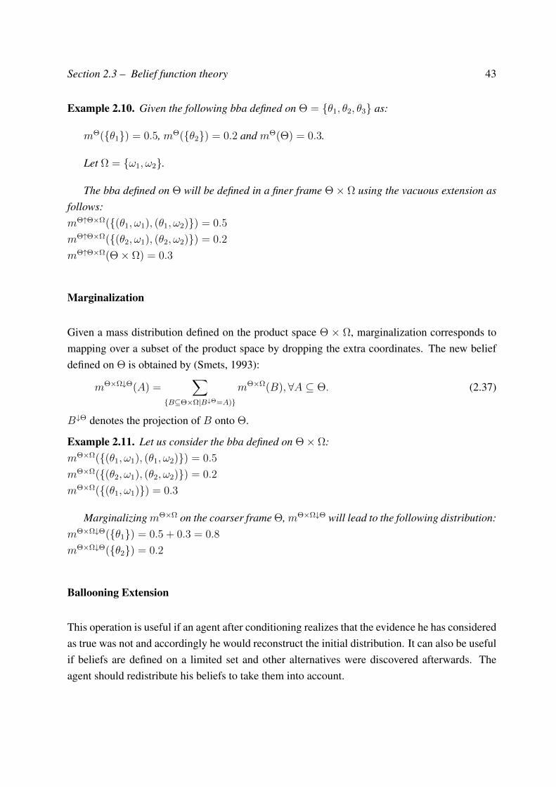
Section 2.3 – Belief function theory 43
Example 2.10. Given the following bba defined on Θ = θ1, θ2, θ3 as:
mΘ(θ1) = 0.5, mΘ(θ2) = 0.2 and mΘ(Θ) = 0.3.
Let Ω = ω1, ω2.
The bba defined on Θ will be defined in a finer frame Θ× Ω using the vacuous extension asfollows:mΘ↑Θ×Ω((θ1, ω1), (θ1, ω2)) = 0.5
mΘ↑Θ×Ω((θ2, ω1), (θ2, ω2)) = 0.2
mΘ↑Θ×Ω(Θ× Ω) = 0.3
Marginalization
Given a mass distribution defined on the product space Θ × Ω, marginalization corresponds tomapping over a subset of the product space by dropping the extra coordinates. The new beliefdefined on Θ is obtained by (Smets, 1993):
mΘ×Ω↓Θ(A) =∑
B⊆Θ×Ω|B↓Θ=A)
mΘ×Ω(B),∀A ⊆ Θ. (2.37)
B↓Θ denotes the projection of B onto Θ.
Example 2.11. Let us consider the bba defined on Θ× Ω:mΘ×Ω((θ1, ω1), (θ1, ω2)) = 0.5
mΘ×Ω((θ2, ω1), (θ2, ω2)) = 0.2
mΘ×Ω((θ1, ω1)) = 0.3
MarginalizingmΘ×Ω on the coarser frame Θ,mΘ×Ω↓Θ will lead to the following distribution:mΘ×Ω↓Θ(θ1) = 0.5 + 0.3 = 0.8
mΘ×Ω↓Θ(θ2) = 0.2
Ballooning Extension
This operation is useful if an agent after conditioning realizes that the evidence he has consideredas true was not and accordingly he would reconstruct the initial distribution. It can also be usefulif beliefs are defined on a limited set and other alternatives were discovered afterwards. Theagent should redistribute his beliefs to take them into account.
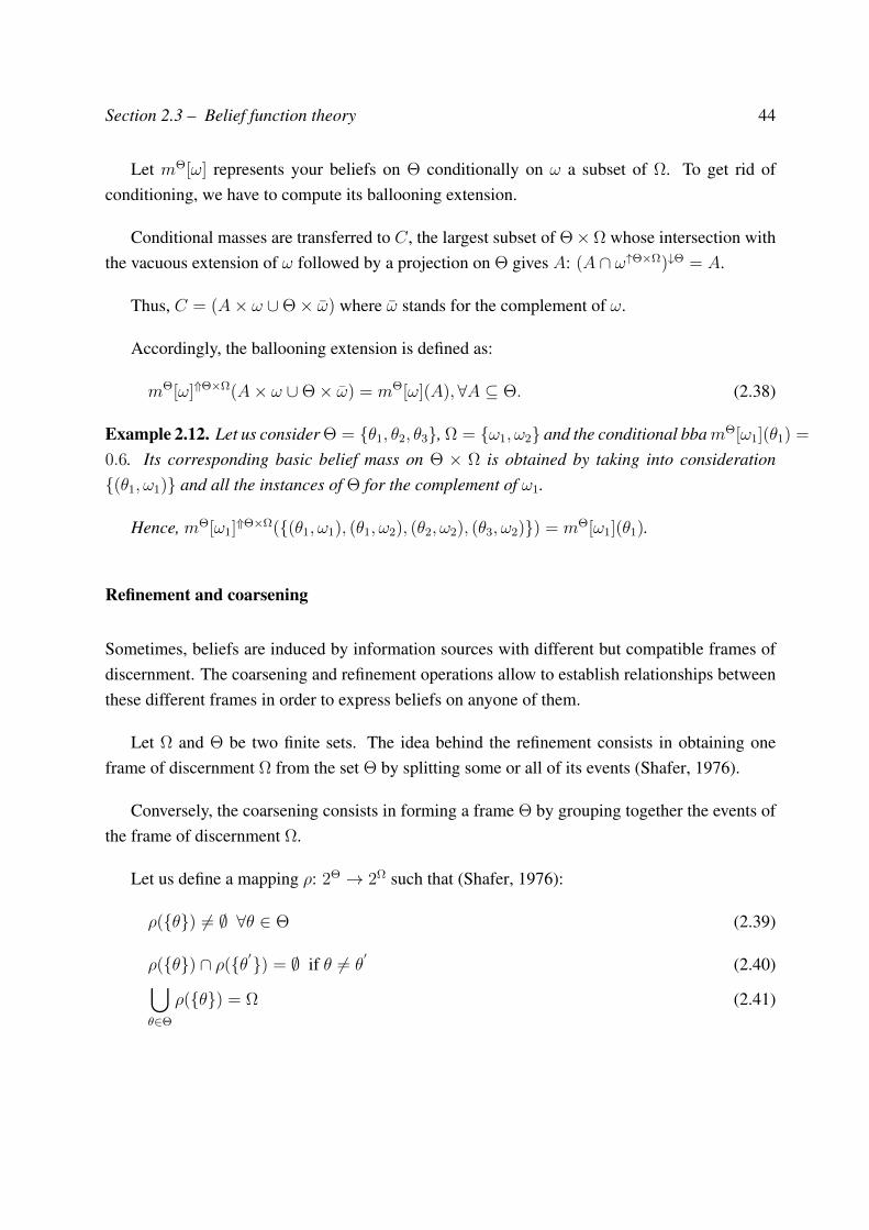
Section 2.3 – Belief function theory 44
Let mΘ[ω] represents your beliefs on Θ conditionally on ω a subset of Ω. To get rid ofconditioning, we have to compute its ballooning extension.
Conditional masses are transferred to C, the largest subset of Θ×Ω whose intersection withthe vacuous extension of ω followed by a projection on Θ gives A: (A ∩ ω↑Θ×Ω)↓Θ = A.
Thus, C = (A× ω ∪Θ× ω) where ω stands for the complement of ω.
Accordingly, the ballooning extension is defined as:
mΘ[ω]⇑Θ×Ω(A× ω ∪Θ× ω) = mΘ[ω](A),∀A ⊆ Θ. (2.38)
Example 2.12. Let us consider Θ = θ1, θ2, θ3, Ω = ω1, ω2 and the conditional bbamΘ[ω1](θ1) =
0.6. Its corresponding basic belief mass on Θ × Ω is obtained by taking into consideration(θ1, ω1) and all the instances of Θ for the complement of ω1.
Hence, mΘ[ω1]⇑Θ×Ω((θ1, ω1), (θ1, ω2), (θ2, ω2), (θ3, ω2)) = mΘ[ω1](θ1).
Refinement and coarsening
Sometimes, beliefs are induced by information sources with different but compatible frames ofdiscernment. The coarsening and refinement operations allow to establish relationships betweenthese different frames in order to express beliefs on anyone of them.
Let Ω and Θ be two finite sets. The idea behind the refinement consists in obtaining oneframe of discernment Ω from the set Θ by splitting some or all of its events (Shafer, 1976).
Conversely, the coarsening consists in forming a frame Θ by grouping together the events ofthe frame of discernment Ω.
Let us define a mapping ρ: 2Θ → 2Ω such that (Shafer, 1976):
ρ(θ) 6= ∅ ∀θ ∈ Θ (2.39)
ρ(θ) ∩ ρ(θ′) = ∅ if θ 6= θ′
(2.40)⋃θ∈Θ
ρ(θ) = Ω (2.41)
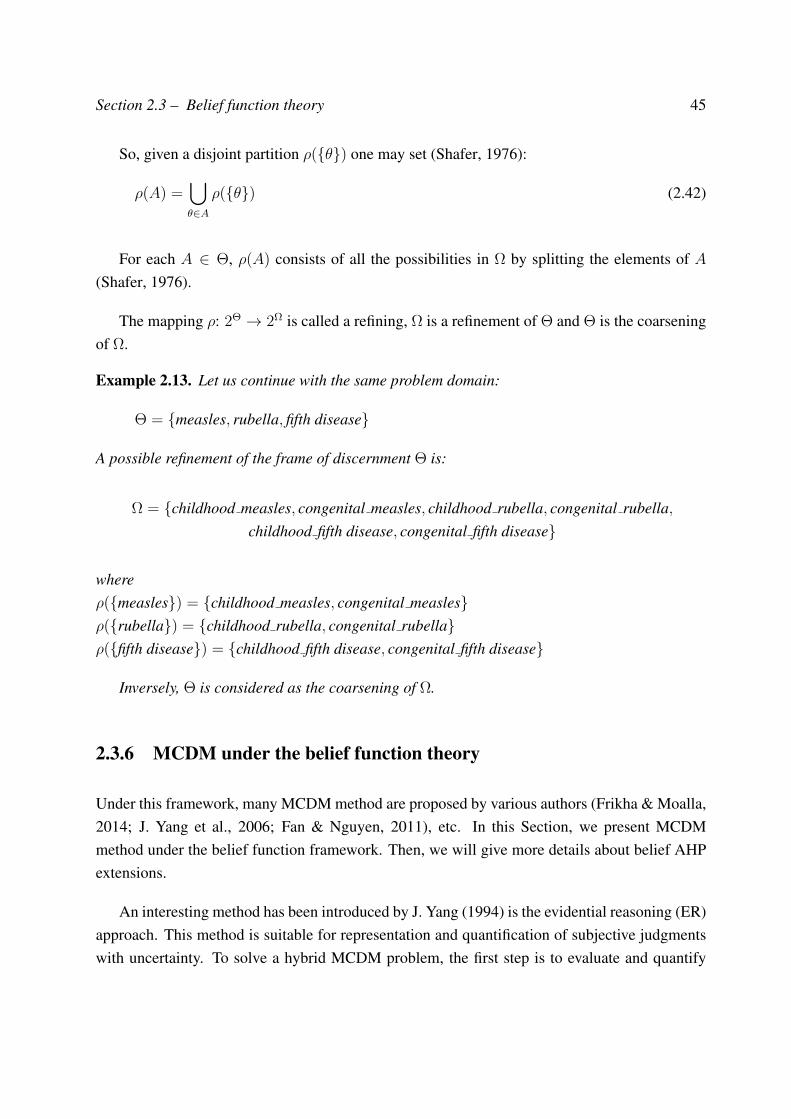
Section 2.3 – Belief function theory 45
So, given a disjoint partition ρ(θ) one may set (Shafer, 1976):
ρ(A) =⋃θ∈A
ρ(θ) (2.42)
For each A ∈ Θ, ρ(A) consists of all the possibilities in Ω by splitting the elements of A(Shafer, 1976).
The mapping ρ: 2Θ → 2Ω is called a refining, Ω is a refinement of Θ and Θ is the coarseningof Ω.
Example 2.13. Let us continue with the same problem domain:
Θ = measles, rubella, fifth disease
A possible refinement of the frame of discernment Θ is:
Ω = childhood measles, congenital measles, childhood rubella, congenital rubella,childhood fifth disease, congenital fifth disease
whereρ(measles) = childhood measles, congenital measlesρ(rubella) = childhood rubella, congenital rubellaρ(fifth disease) = childhood fifth disease, congenital fifth disease
Inversely, Θ is considered as the coarsening of Ω.
2.3.6 MCDM under the belief function theory
Under this framework, many MCDM method are proposed by various authors (Frikha & Moalla,2014; J. Yang et al., 2006; Fan & Nguyen, 2011), etc. In this Section, we present MCDMmethod under the belief function framework. Then, we will give more details about belief AHPextensions.
An interesting method has been introduced by J. Yang (1994) is the evidential reasoning (ER)approach. This method is suitable for representation and quantification of subjective judgmentswith uncertainty. To solve a hybrid MCDM problem, the first step is to evaluate and quantify
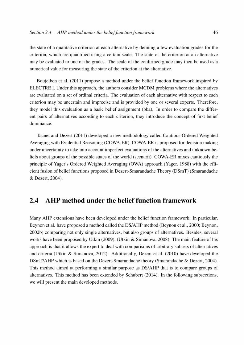
Section 2.4 – AHP method under the belief function framework 46
the state of a qualitative criterion at each alternative by defining a few evaluation grades for thecriterion, which are quantified using a certain scale. The state of the criterion at an alternativemay be evaluated to one of the grades. The scale of the confirmed grade may then be used as anumerical value for measuring the state of the criterion at the alternative.
Boujelben et al. (2011) propose a method under the belief function framework inspired byELECTRE I. Under this approach, the authors consider MCDM problems where the alternativesare evaluated on a set of ordinal criteria. The evaluation of each alternative with respect to eachcriterion may be uncertain and imprecise and is provided by one or several experts. Therefore,they model this evaluation as a basic belief assignment (bba). In order to compare the differ-ent pairs of alternatives according to each criterion, they introduce the concept of first beliefdominance.
Tacnet and Dezert (2011) developed a new methodology called Cautious Ordered WeightedAveraging with Evidential Reasoning (COWA-ER). COWA-ER is proposed for decision makingunder uncertainty to take into account imperfect evaluations of the alternatives and unknown be-liefs about groups of the possible states of the world (scenarii). COWA-ER mixes cautiously theprinciple of Yager’s Ordered Weighted Averaging (OWA) approach (Yager, 1988) with the effi-cient fusion of belief functions proposed in Dezert-Smarandache Theory (DSmT) (Smarandache& Dezert, 2004).
2.4 AHP method under the belief function framework
Many AHP extensions have been developed under the belief function framework. In particular,Beynon et al. have proposed a method called the DS/AHP method (Beynon et al., 2000; Beynon,2002b) comparing not only single alternatives, but also groups of alternatives. Besides, severalworks have been proposed by Utkin (2009), (Utkin & Simanova, 2008). The main feature of hisapproach is that it allows the expert to deal with comparisons of arbitrary subsets of alternativesand criteria (Utkin & Simanova, 2012). Additionally, Dezert et al. (2010) have developed theDSmT/AHP which is based on the Dezert-Smarandache theory (Smarandache & Dezert, 2004).This method aimed at performing a similar purpose as DS/AHP that is to compare groups ofalternatives. This method has been extended by Schubert (2014). In the following subsections,we will present the main developed methods.
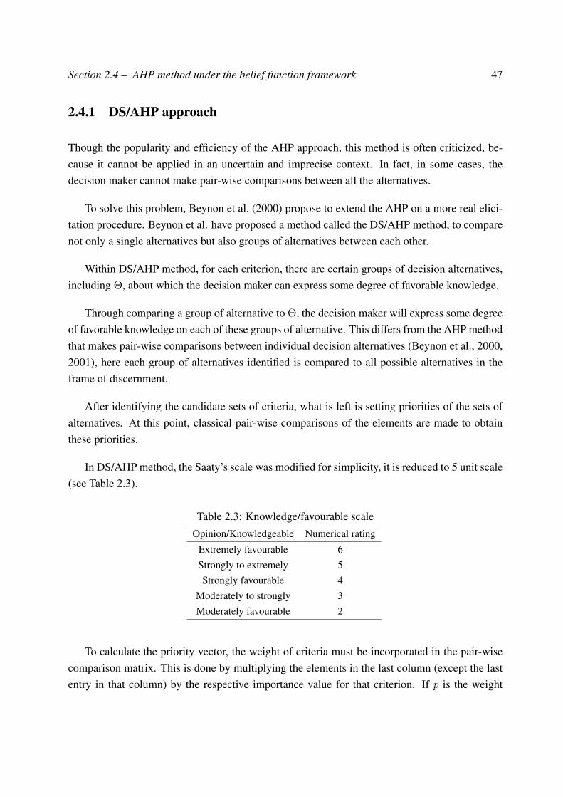
Section 2.4 – AHP method under the belief function framework 47
2.4.1 DS/AHP approach
Though the popularity and efficiency of the AHP approach, this method is often criticized, be-cause it cannot be applied in an uncertain and imprecise context. In fact, in some cases, thedecision maker cannot make pair-wise comparisons between all the alternatives.
To solve this problem, Beynon et al. (2000) propose to extend the AHP on a more real elici-tation procedure. Beynon et al. have proposed a method called the DS/AHP method, to comparenot only a single alternatives but also groups of alternatives between each other.
Within DS/AHP method, for each criterion, there are certain groups of decision alternatives,including Θ, about which the decision maker can express some degree of favorable knowledge.
Through comparing a group of alternative to Θ, the decision maker will express some degreeof favorable knowledge on each of these groups of alternative. This differs from the AHP methodthat makes pair-wise comparisons between individual decision alternatives (Beynon et al., 2000,2001), here each group of alternatives identified is compared to all possible alternatives in theframe of discernment.
After identifying the candidate sets of criteria, what is left is setting priorities of the sets ofalternatives. At this point, classical pair-wise comparisons of the elements are made to obtainthese priorities.
In DS/AHP method, the Saaty’s scale was modified for simplicity, it is reduced to 5 unit scale(see Table 2.3).
Table 2.3: Knowledge/favourable scaleOpinion/Knowledgeable Numerical rating
Extremely favourable 6Strongly to extremely 5Strongly favourable 4
Moderately to strongly 3Moderately favourable 2
To calculate the priority vector, the weight of criteria must be incorporated in the pair-wisecomparison matrix. This is done by multiplying the elements in the last column (except the lastentry in that column) by the respective importance value for that criterion. If p is the weight
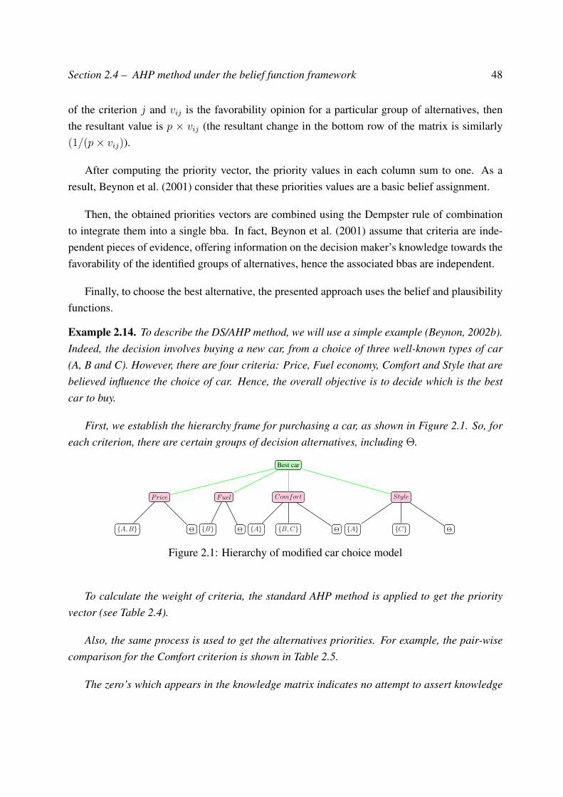
Section 2.4 – AHP method under the belief function framework 48
of the criterion j and vij is the favorability opinion for a particular group of alternatives, thenthe resultant value is p × vij (the resultant change in the bottom row of the matrix is similarly(1/(p× vij)).
After computing the priority vector, the priority values in each column sum to one. As aresult, Beynon et al. (2001) consider that these priorities values are a basic belief assignment.
Then, the obtained priorities vectors are combined using the Dempster rule of combinationto integrate them into a single bba. In fact, Beynon et al. (2001) assume that criteria are inde-pendent pieces of evidence, offering information on the decision maker’s knowledge towards thefavorability of the identified groups of alternatives, hence the associated bbas are independent.
Finally, to choose the best alternative, the presented approach uses the belief and plausibilityfunctions.
Example 2.14. To describe the DS/AHP method, we will use a simple example (Beynon, 2002b).Indeed, the decision involves buying a new car, from a choice of three well-known types of car(A, B and C). However, there are four criteria: Price, Fuel economy, Comfort and Style that arebelieved influence the choice of car. Hence, the overall objective is to decide which is the bestcar to buy.
First, we establish the hierarchy frame for purchasing a car, as shown in Figure 2.1. So, foreach criterion, there are certain groups of decision alternatives, including Θ.
Best car
Price
A,B Θ
Fuel
B Θ
Comfort
A B,C Θ
Style
A C Θ
Figure 2.1: Hierarchy of modified car choice model
To calculate the weight of criteria, the standard AHP method is applied to get the priorityvector (see Table 2.4).
Also, the same process is used to get the alternatives priorities. For example, the pair-wisecomparison for the Comfort criterion is shown in Table 2.5.
The zero’s which appears in the knowledge matrix indicates no attempt to assert knowledge
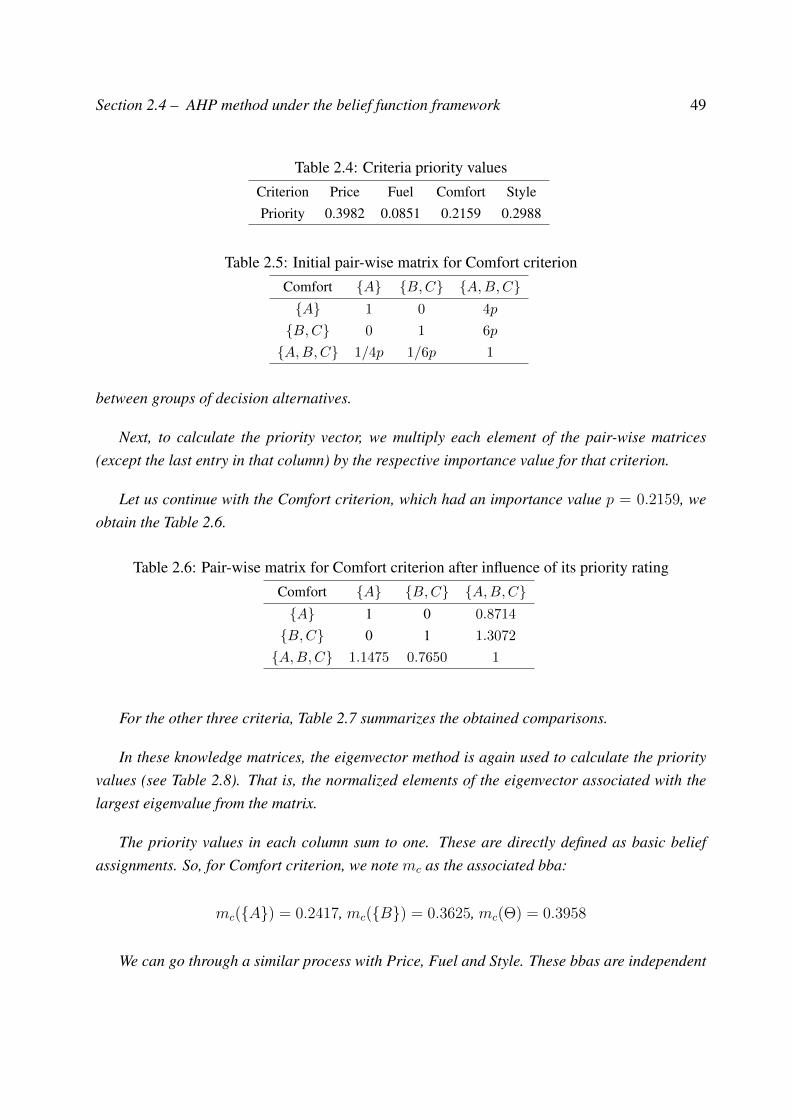
Section 2.4 – AHP method under the belief function framework 49
Table 2.4: Criteria priority valuesCriterion Price Fuel Comfort StylePriority 0.3982 0.0851 0.2159 0.2988
Table 2.5: Initial pair-wise matrix for Comfort criterionComfort A B,C A,B,CA 1 0 4p
B,C 0 1 6p
A,B,C 1/4p 1/6p 1
between groups of decision alternatives.
Next, to calculate the priority vector, we multiply each element of the pair-wise matrices(except the last entry in that column) by the respective importance value for that criterion.
Let us continue with the Comfort criterion, which had an importance value p = 0.2159, weobtain the Table 2.6.
Table 2.6: Pair-wise matrix for Comfort criterion after influence of its priority ratingComfort A B,C A,B,CA 1 0 0.8714
B,C 0 1 1.3072
A,B,C 1.1475 0.7650 1
For the other three criteria, Table 2.7 summarizes the obtained comparisons.
In these knowledge matrices, the eigenvector method is again used to calculate the priorityvalues (see Table 2.8). That is, the normalized elements of the eigenvector associated with thelargest eigenvalue from the matrix.
The priority values in each column sum to one. These are directly defined as basic beliefassignments. So, for Comfort criterion, we note mc as the associated bba:
mc(A) = 0.2417, mc(B) = 0.3625, mc(Θ) = 0.3958
We can go through a similar process with Price, Fuel and Style. These bbas are independent

Section 2.4 – AHP method under the belief function framework 50
Table 2.7: Pair-wise matrix for Price, Fuel and StylePrice A,B Θ
A,B 1 6p
Θ 1/6p 1
Fuel B Θ
B 1 3p
Θ 1/3p 1
Style A C Θ
A 1 0 5p
C 0 1 2p
Θ 1/5p 1/2p 1
Table 2.8: Priority valuesPrice Priority Fuel Priority Comfort Priority Style Priority
A,B 0.7049 B 0.2034 A 0.2417 A 0.4261Θ 0.2951 Θ 0.7966 B,C 0.3625 C 0.1705
Θ 0.3958 Θ 0.4034
pieces of evidence. Hence, the associated bba are independent. So, we use the Dempster rule ofcombination to get a single bba and the resulting bba is shown in Table 2.9.
Table 2.9: The bba mcar after combining all evidenceDA A B C A,B B,C Θ
mcar 0.4309 0.2312 0.0511 0.1650 0.0527 0.0691
Now, we can calculate the belief and plausibility functions and we obtain the following Table2.10
If we consider the focal element A, then there is a small amount of evidence in favour aswell as against the hypothesis A being the best car. For C the table shows strong evidenceagainst being the best choice. Interestingly the set A,B shows strong evidence in favour ofincluding within its elements the best choice of car.
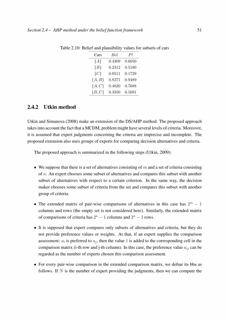
Section 2.4 – AHP method under the belief function framework 51
Table 2.10: Belief and plausibility values for subsets of carsCars Bel P l
A 0.4309 0.6650
B 0.2312 0.5180
C 0.0511 0.1729
A,B 0.8271 0.9489
A,C 0.4820 0.7688
B,C 0.3350 0.5691
2.4.2 Utkin method
Utkin and Simanova (2008) make an extension of the DS/AHP method. The proposed approachtakes into account the fact that a MCDM, problem might have several levels of criteria. Moreover,it is assumed that expert judgments concerning the criteria are imprecise and incomplete. Theproposed extension also uses groups of experts for comparing decision alternatives and criteria.
The proposed approach is summarized in the following steps (Utkin, 2009):
• We suppose that there is a set of alternatives consisting of m and a set of criteria consistingof n. An expert chooses some subset of alternatives and compares this subset with anothersubset of alternatives with respect to a certain criterion. In the same way, the decisionmaker chooses some subset of criteria from the set and compares this subset with anothergroup of criteria.
• The extended matrix of pair-wise comparisons of alternatives in this case has 2m − 1
columns and rows (the empty set is not considered here). Similarly, the extended matrixof comparisons of criteria has 2n − 1 columns and 2n − 1 rows.
• It is supposed that expert compares only subsets of alternatives and criteria, but they donot provide preference values or weights. At that, if an expert supplies the comparisonassessment: ai is preferred to aj , then the value 1 is added to the corresponding cell in thecomparison matrix (i-th row and j-th column). In this case, the preference value aij can beregarded as the number of experts chosen this comparison assessment.
• For every pair-wise comparison in the extended comparison matrix, we define its bba asfollows. If N is the number of expert providing the judgments, then we can compute the
Section 2.4 – AHP method under the belief function framework 52
bba by:
m((ai, aj)) =aijN
(2.43)
Example 2.15. Let us study a decision problem where the decision maker has to choose whichone of three alternatives evaluated based on two criteria c1 and c2. Suppose that 15 expertsprovide preferences concerning criteria as shown in Table 2.11.
Table 2.11: Expert preferences related to criteriac1 c2 c1, c2D1 D2 D3
ck 6 4 5
m(Dk)615
415
515
By introducing the special algebra of sets of preferences, a combination procedure is definedto aggregate the references for alternatives and for criteria. At this level, the DS/AHP methodis applied. This method is used to identify the most favorable subsets from the available set ofcriteria or alternatives. Then, the second task is to use the beliefBel and plausibility Pl functionsof preferences as a lower and upper probabilities. Therefore, Utkin et al. solve this problem as alinear programming problems.
2.4.3 ER-MCDM method
This framework called ER-MCDM mixes the AHP and uncertainty theories including fuzzysets, possibility and belief function theories (Tacnet et al., 2010, 2011). The principle of theER-MCDM methodology is to use AHP to analyze the decision problem and to replace theaggregation step by two successive fusion processes. Its main objective is to take into accountboth information imperfection, source reliability and conflict.
ER-MCDM is described as follows:
• Analyzing the decision problem through a hierarchical structure.
• Defining the evaluation classes for decision through a common frame of discernment.
• Evaluating the qualitative or quantitative criteria.
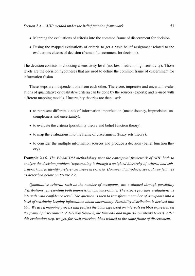
Section 2.4 – AHP method under the belief function framework 53
• Mapping the evaluations of criteria into the common frame of discernment for decision.
• Fusing the mapped evaluations of criteria to get a basic belief assignment related to theevaluations classes of decision (frame of discernment for decision).
The decision consists in choosing a sensitivity level (no, low, medium, high sensitivity). Thoselevels are the decision hypotheses that are used to define the common frame of discernment forinformation fusion.
These steps are independent one from each other. Therefore, imprecise and uncertain evalu-ations of quantitative or qualitative criteria can be done by the sources (experts) and re-used withdifferent mapping models. Uncertainty theories are then used:
• to represent different kinds of information imperfection (unconsistency, imprecision, un-completness and uncertainty).
• to evaluate the criteria (possibility theory and belief function theory).
• to map the evaluations into the frame of discernment (fuzzy sets theory).
• to consider the multiple information sources and produce a decision (belief function the-ory).
Example 2.16. The ER-MCDM methodology uses the conceptual framework of AHP both toanalyze the decision problem (representing it through a weighted hierarchy of criteria and sub-criteria) and to identify preferences between criteria. However, it introduces several new featuresas described below on Figure 2.2.
Quantitative criteria, such as the number of occupants, are evaluated through possibilitydistributions representing both imprecision and uncertainty. The expert provides evaluations asintervals with confidence level. The question is then to transform a number of occupants into alevel of sensitivity keeping information about uncertainty. Possibility distribution is derived intobba. We use a mapping process that project the bbas expressed on intervals on bbas expressed onthe frame of discernment of decision (low-LS, medium-MS and high-HS sensitivity levels). Afterthis evaluation step, we get, for each criterion, bbas related to the same frame of discernment.
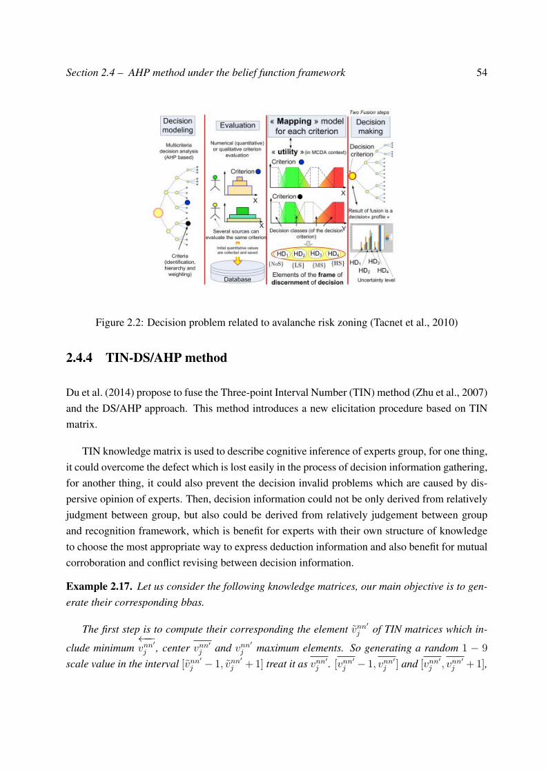
Section 2.4 – AHP method under the belief function framework 54
Figure 2.2: Decision problem related to avalanche risk zoning (Tacnet et al., 2010)
2.4.4 TIN-DS/AHP method
Du et al. (2014) propose to fuse the Three-point Interval Number (TIN) method (Zhu et al., 2007)and the DS/AHP approach. This method introduces a new elicitation procedure based on TINmatrix.
TIN knowledge matrix is used to describe cognitive inference of experts group, for one thing,it could overcome the defect which is lost easily in the process of decision information gathering,for another thing, it could also prevent the decision invalid problems which are caused by dis-persive opinion of experts. Then, decision information could not be only derived from relativelyjudgment between group, but also could be derived from relatively judgement between groupand recognition framework, which is benefit for experts with their own structure of knowledgeto choose the most appropriate way to express deduction information and also benefit for mutualcorroboration and conflict revising between decision information.
Example 2.17. Let us consider the following knowledge matrices, our main objective is to gen-erate their corresponding bbas.
The first step is to compute their corresponding the element vnn′
j of TIN matrices which in-
clude minimum←−−vnn
′j , center vnn
′j and vnn
′j maximum elements. So generating a random 1 − 9
scale value in the interval [vnn′
j − 1, vnn′
j +1] treat it as vnn′j . [vnn′
j − 1, vnn′
j ] and [vnn′
j , vnn′
j +1],
Section 2.5 – Conclusion 55
treat them as←−−vnn
′j and vnn
′j .
The TIN knowledge matrices generated by above process is as shown in Figure 2.3.
Figure 2.3: The corresponding TIN knowledge matrices
Then, according to TIN-DS/AHP, the corresponding bbas are solved and the decision is makeusing pignistic probabilities.
2.5 Conclusion
In this Chapter, we have presented an overview of the main developed AHP approaches underuncertain theories. In the second part, we have presented the basic concepts of belief functiontheory as understood in the Transferable Belief Model. This presentation shows that the belieffunction theory provides a convenient tool to handle uncertainty in decision problems, especially

Section 2.5 – Conclusion 56
within Multi-Criteria Decision Making methods. For this reason, this theory will be used as atool to formalize different forms of uncertainty under the AHP model.
As we have described, AHP method has some limits. Therefore, in the next Chapter, we willpresent belief AHP method as a possible solution to deal with uncertainty using the belief func-tion theory framework. An improvement of this latter will also be proposed via new elicitationtechniques.
Part II presents the contributions of this Thesis. This partfocuses on presenting our newly developed approachessolving some of the AHP mentioned limitations. The twofirst Chapters present new approaches based on a quantita-tive scale under the belief function framework. Secondly,the next two Chapters detail solutions dealing with qual-itative elicitation technique. The proposed latter methodsare based on a new qualitative reasoning approach that de-rive crisp priorities from qualitative judgments.
PART II:
CONTRIBUTIONS
57
Chapter 3Modeling dependency betweenalternatives and criteria
3.1 Introduction
Uncertainty is a source of complexity in decision making. There are various forms that may arisein multi-criteria decision making (MCDM), in particular the Analytic Hierarchy Process (AHP),from impression to lack of knowledge or ignorance. As described in the previous Chapter, at onelevel there is an uncertainty about alternatives that appear in the identification of the candidatealternatives. At another level, there is an uncertainty about the ability of the selected criteria toadequately represent the objective that the decision maker tries to achieve. However, imperfec-tion may also be in the evaluation process. So, variability in all these factors has the potential toaffect the ranking of alternatives of a MCDM problem.
Our objectives through this research are to handle the different types of uncertainty in orderto solve more complex MCDM problems. Hence, in this Chapter, we will introduce a newapproach, which is able to model dependency between alternatives and criteria.
Since the main purpose is to rank alternatives, the proposed methodology is constructed uponthe basis of the AHP method. As mentioned previously, AHP is a pair-wise comparison tech-nique, which can model a complex problem in a unidirectional hierarchical structure assumingthat there are no interdependencies between or within the levels. It assumes that there are no rela-
58
Section 3.2 – Belief AHP method 59
tionships between the alternatives and criteria. However, at the alternative level, when modelinghis assessment, the decision maker expresses his evaluation regarding each criterion. In otherwords, the alternative preferences depend on each criterion, which has an effect on the chosenalternatives.
Therefore, a new MCDM method has been developed as part of this research. The mainaim of the proposed approach is to find a way to model the relationship between alternativesand criteria. While the methodology handles the existence of dependency between criteria andalternatives, it can also incorporate the belief function theory in order to correctly reflect thedecision behavior of the expert. First of all, our method, called belief AHP, deals with uncertaintyinto two levels namely the criterion and alternative. So, the decision maker may express hispreferences in groups of criteria and alternatives instead of a single one. In other ways andas an extension of the belief AHP approach, our second solution is introduced to represent theinfluences of the criteria on the evaluation of alternatives.
The rest of this Chapter is organized as follows: in Section 3.2, we introduce belief AHP, aMCDM approach that combines the belief function theory with the AHP method. Section 3.3investigates the relationship between alternatives and criteria and presents our new belief AHPmethod where beliefs are expressed in terms of conditional mass distributions. In the last Section(Section 3.4), we present some experimental studies.
3.2 Belief AHP method
3.2.1 Introduction
This Section is dedicated to the presentation of the basic steps needed to ensure the ranking ofalternatives in an uncertain environment. In this context, we introduce our belief AHP approachwhich is a combination of AHP method and the belief function theory. A first work has been in-troduced in Ennaceur et al. (2011). Its main idea is to compare groups of criteria and alternatives.Then, it represents the weights of criteria by a reliability measure and the alternatives prioritiesusing basic belief assignments (bba).
This Section illustrates belief AHP method and investigates its fundamentals steps. Exampleswill be given to illustrate the approach.
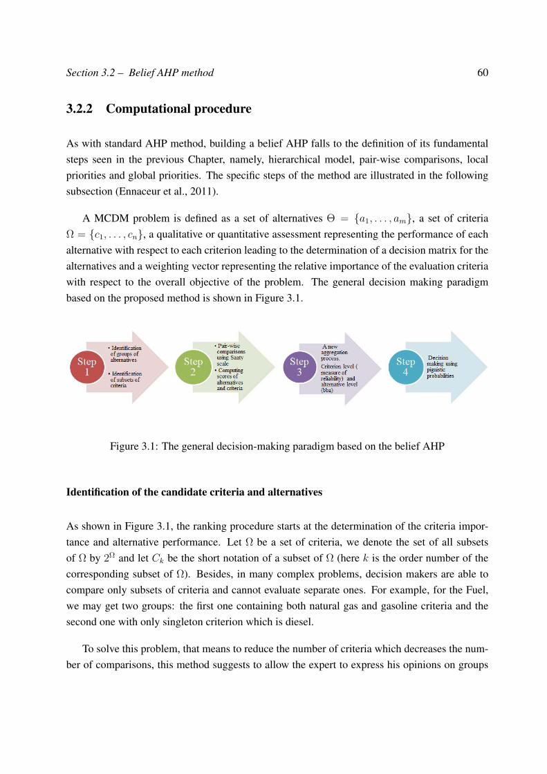
Section 3.2 – Belief AHP method 60
3.2.2 Computational procedure
As with standard AHP method, building a belief AHP falls to the definition of its fundamentalsteps seen in the previous Chapter, namely, hierarchical model, pair-wise comparisons, localpriorities and global priorities. The specific steps of the method are illustrated in the followingsubsection (Ennaceur et al., 2011).
A MCDM problem is defined as a set of alternatives Θ = a1, . . . , am, a set of criteriaΩ = c1, . . . , cn, a qualitative or quantitative assessment representing the performance of eachalternative with respect to each criterion leading to the determination of a decision matrix for thealternatives and a weighting vector representing the relative importance of the evaluation criteriawith respect to the overall objective of the problem. The general decision making paradigmbased on the proposed method is shown in Figure 3.1.
Figure 3.1: The general decision-making paradigm based on the belief AHP
Identification of the candidate criteria and alternatives
As shown in Figure 3.1, the ranking procedure starts at the determination of the criteria impor-tance and alternative performance. Let Ω be a set of criteria, we denote the set of all subsetsof Ω by 2Ω and let Ck be the short notation of a subset of Ω (here k is the order number of thecorresponding subset of Ω). Besides, in many complex problems, decision makers are able tocompare only subsets of criteria and cannot evaluate separate ones. For example, for the Fuel,we may get two groups: the first one containing both natural gas and gasoline criteria and thesecond one with only singleton criterion which is diesel.
To solve this problem, that means to reduce the number of criteria which decreases the num-ber of comparisons, this method suggests to allow the expert to express his opinions on groups
Section 3.2 – Belief AHP method 61
of criteria instead of single one. So, the expert chooses these subsets by assuming that criteriahaving the same degree of preference are grouped together. For instance, if an expert identifies agroup of criteria, then we could suppose that all of them have the same importance. Thus, thesegroups can be defined as:
∀ k, j|Ck, Cj ∈ 2Ω, Ck ∩ Cj = ∅ and⋃j
Cj = Ω (with Cj exclusive). (3.1)
Since we are not performing pair-wise comparisons of criteria but relating to groups of cri-teria, these sets should not consider a criterion in common. If one criterion is included in twogroups, then each group will give a different level of favorability and the expert judgment couldbe inconsistent.
Like the criterion level, the proposed model denotes the set of all subsets of alternatives Θ
by 2Θ and let Ak be the short notation of a subset of A, i.e., Ak ⊆ Θ. At this level, this methodsuggests to not necessarily consider all of them but just to choose groups of those alternatives.One of the possible solutions of this task is to use the DS/AHP method (Beynon et al., 2000).Besides, the proposed approach applies the same hypothesis assumed in DS/AHP to identify thesubsets of alternatives (see Chapter 2). The decision maker compares not only a single one butalso sets of alternatives between each other.
Example 3.1. To describe this approach, we consider the problem of purchasing a car. Supposethat this problem involves four criteria: Ω = Price (c1), Style (c2), Fuel (c3), Reliability (c4)and three selected alternatives: Θ = Peugeot (p),Renault (r),Ford (f).
The expert can identify the following subsets c1, c4 and c2, c3. He assumed that thetwo criteria c2 and c3 have the same degree of importance. Therefore, they are grouped together.
Similarly to the criterion level, the judgments between decision alternatives over differentcriteria are dealt within an identical manner. For example, to evaluate the alternatives accordingto the criterion c1, the expert is asked to evaluate the following subsets of alternatives: p andp, r, f.
The belief AHP hierarchy is then constructed as shown in Figure 3.2.

Section 3.2 – Belief AHP method 62
Best car
c1
p Θ
c2, c3
c2
p r, f Θ
c3
r Θ
c4
f Θ
Figure 3.2: The belied AHP Hierarchy of car choice model
Pair-wise comparisons and preference elicitation
Once the sets of criteria and alternatives are defined, the expert tries to specify his assessments.In this study, the proposed model has adopted the Saaty’s scale to evaluate the importance of pairsof grouped elements in terms of their contribution (see Step 2 in Figure 3.1). Thus, the priorityvectors are then generated using the eigenvector method and the standard consistency index ischosen in order to ensure that belief AHP’s pair-wise comparison matrices are consistent.
Example 3.2. If we consider the previous example where: c1, c4 and c2, c3 are the groupsof criteria which belong to the power set of 2Ω. The decision maker can define his preferences byusing the pair-wise comparison of the following type “How important is criterion c1 relativeto criterion c4 ?”. To respond to this question, the expert uses Saaty’s scale expressing theintensity of the preference for one criterion versus another (see Table 3.1).
Table 3.1: The weights assigned to the criteria according to the expert’s opinionCriteria c1 c4 c2, c3 Priority
c1 1 2 6 0.58
c4 12 1 4 0.32
c2, c3 16
14 1 0.1
At the alternative level, a sample matrix for the Price criterion, for example, being shown inTable 3.2.
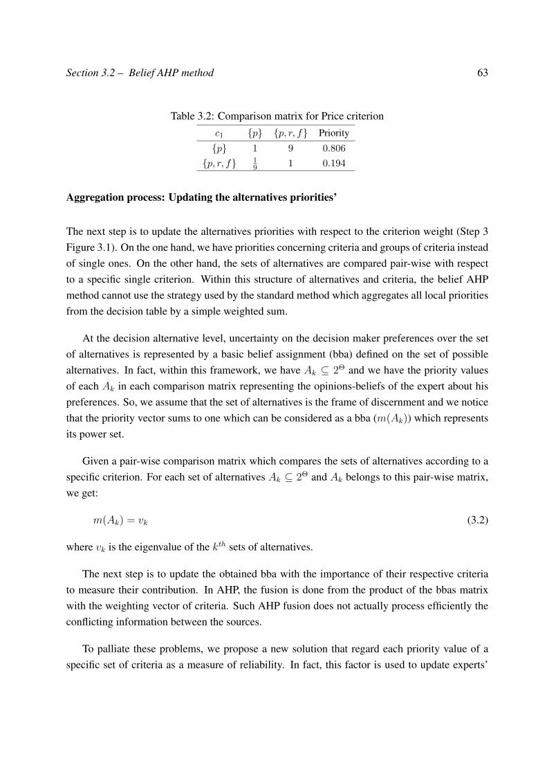
Section 3.2 – Belief AHP method 63
Table 3.2: Comparison matrix for Price criterionc1 p p, r, f Priority
p 1 9 0.806
p, r, f 19 1 0.194
Aggregation process: Updating the alternatives priorities’
The next step is to update the alternatives priorities with respect to the criterion weight (Step 3Figure 3.1). On the one hand, we have priorities concerning criteria and groups of criteria insteadof single ones. On the other hand, the sets of alternatives are compared pair-wise with respectto a specific single criterion. Within this structure of alternatives and criteria, the belief AHPmethod cannot use the strategy used by the standard method which aggregates all local prioritiesfrom the decision table by a simple weighted sum.
At the decision alternative level, uncertainty on the decision maker preferences over the setof alternatives is represented by a basic belief assignment (bba) defined on the set of possiblealternatives. In fact, within this framework, we have Ak ⊆ 2Θ and we have the priority valuesof each Ak in each comparison matrix representing the opinions-beliefs of the expert about hispreferences. So, we assume that the set of alternatives is the frame of discernment and we noticethat the priority vector sums to one which can be considered as a bba (m(Ak)) which representsits power set.
Given a pair-wise comparison matrix which compares the sets of alternatives according to aspecific criterion. For each set of alternatives Ak ⊆ 2Θ and Ak belongs to this pair-wise matrix,we get:
m(Ak) = vk (3.2)
where vk is the eigenvalue of the kth sets of alternatives.
The next step is to update the obtained bba with the importance of their respective criteriato measure their contribution. In AHP, the fusion is done from the product of the bbas matrixwith the weighting vector of criteria. Such AHP fusion does not actually process efficiently theconflicting information between the sources.
To palliate these problems, we propose a new solution that regard each priority value of aspecific set of criteria as a measure of reliability. In fact, this factor is used to update experts’
Section 3.2 – Belief AHP method 64
beliefs (bba) by taking into account the important of each set of criteria. The idea is then tomeasure most heavily the bba evaluated according to the most important criteria and converselyfor the less important ones.
If we have Ck (as defined above) as a subset of criteria, then we get βk its correspondingmeasure of reliability:
βk =ωkωmax
(3.3)
where wk is the eigenvalue of the kth sets of criteria and ωmax is the maximum eigenvalue suchas:
ωmax = maxk∈[1:l]ωk (3.4)
where l is the number of subsets of criteria.
Consequently, two cases will be presented. First, if the reliability factor represents a singlecriterion, then the corresponding bba will be directly discounted.
If Ck is a singleton criterion, then we apply the discounting rule and we get:
mαkCk
(Aj) = βk.mCk(Aj), ∀Aj ⊂ Θ (3.5)
mαkCk
(Θ) = (1− βk) + βk.mCk(Θ) (3.6)
where Aj a subset of alternatives that are evaluated with respect to the criterion Ck, mCk(Ak)
the relative bbm for the subset Ak, βk its corresponding measure of reliability and we denoteαk = 1− βk.
Second, if this factor represents a group of criteria, their corresponding bbas must be com-bined using the conjunctive rule (see Equation 2.13), then it will be discounted by the measureof reliability relative to this group of criteria.
Let Ck a subset of criteria and ci ∈ Ck, then we apply the conjunctive rule of combination toobtain mCk
:
mCk= ∩©mci , i = 1, . . . , h (3.7)
where h is the number of elements of a specific group of criteria Ck and ci is a singleton criterion.
Finally, these obtained bbas (mCk) will be discounted by their corresponding measure of
reliability βk. We apply the same idea used in Equations 3.5 and 3.6, to get mαkCk
.
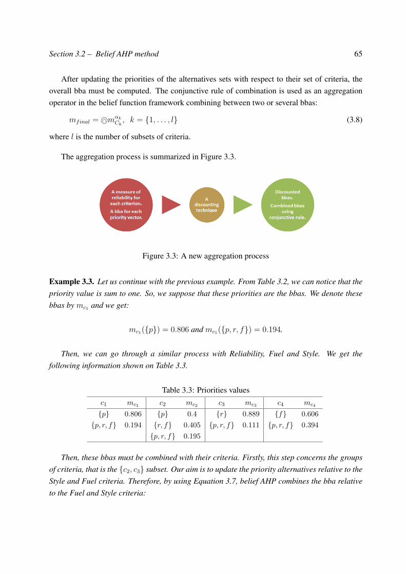
Section 3.2 – Belief AHP method 65
After updating the priorities of the alternatives sets with respect to their set of criteria, theoverall bba must be computed. The conjunctive rule of combination is used as an aggregationoperator in the belief function framework combining between two or several bbas:
mfinal = ∩©mαkCk, k = 1, . . . , l (3.8)
where l is the number of subsets of criteria.
The aggregation process is summarized in Figure 3.3.
Figure 3.3: A new aggregation process
Example 3.3. Let us continue with the previous example. From Table 3.2, we can notice that thepriority value is sum to one. So, we suppose that these priorities are the bbas. We denote thesebbas by mc1 and we get:
mc1(p) = 0.806 and mc1(p, r, f) = 0.194.
Then, we can go through a similar process with Reliability, Fuel and Style. We get thefollowing information shown on Table 3.3.
Table 3.3: Priorities valuesc1 mc1 c2 mc2 c3 mc3 c4 mc4
p 0.806 p 0.4 r 0.889 f 0.606
p, r, f 0.194 r, f 0.405 p, r, f 0.111 p, r, f 0.394
p, r, f 0.195
Then, these bbas must be combined with their criteria. Firstly, this step concerns the groupsof criteria, that is the c2, c3 subset. Our aim is to update the priority alternatives relative to theStyle and Fuel criteria. Therefore, by using Equation 3.7, belief AHP combines the bba relativeto the Fuel and Style criteria:
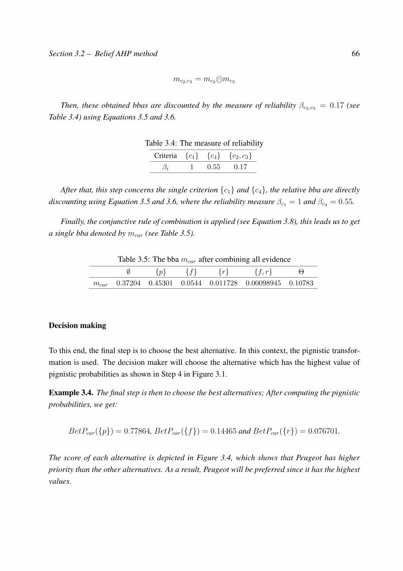
Section 3.2 – Belief AHP method 66
mc2,c3 = mc2 ∩©mc3
Then, these obtained bbas are discounted by the measure of reliability βc2,c3 = 0.17 (seeTable 3.4) using Equations 3.5 and 3.6.
Table 3.4: The measure of reliabilityCriteria c1 c4 c2, c3βi 1 0.55 0.17
After that, this step concerns the single criterion c1 and c4, the relative bba are directlydiscounting using Equation 3.5 and 3.6, where the reliability measure βc1 = 1 and βc4 = 0.55.
Finally, the conjunctive rule of combination is applied (see Equation 3.8), this leads us to geta single bba denoted by mcar (see Table 3.5).
Table 3.5: The bba mcar after combining all evidence∅ p f r f, r Θ
mcar 0.37204 0.45301 0.0544 0.011728 0.00098945 0.10783
Decision making
To this end, the final step is to choose the best alternative. In this context, the pignistic transfor-mation is used. The decision maker will choose the alternative which has the highest value ofpignistic probabilities as shown in Step 4 in Figure 3.1.
Example 3.4. The final step is then to choose the best alternatives; After computing the pignisticprobabilities, we get:
BetPcar(p) = 0.77864, BetPcar(f) = 0.14465 and BetPcar(r) = 0.076701.
The score of each alternative is depicted in Figure 3.4, which shows that Peugeot has higherpriority than the other alternatives. As a result, Peugeot will be preferred since it has the highestvalues.
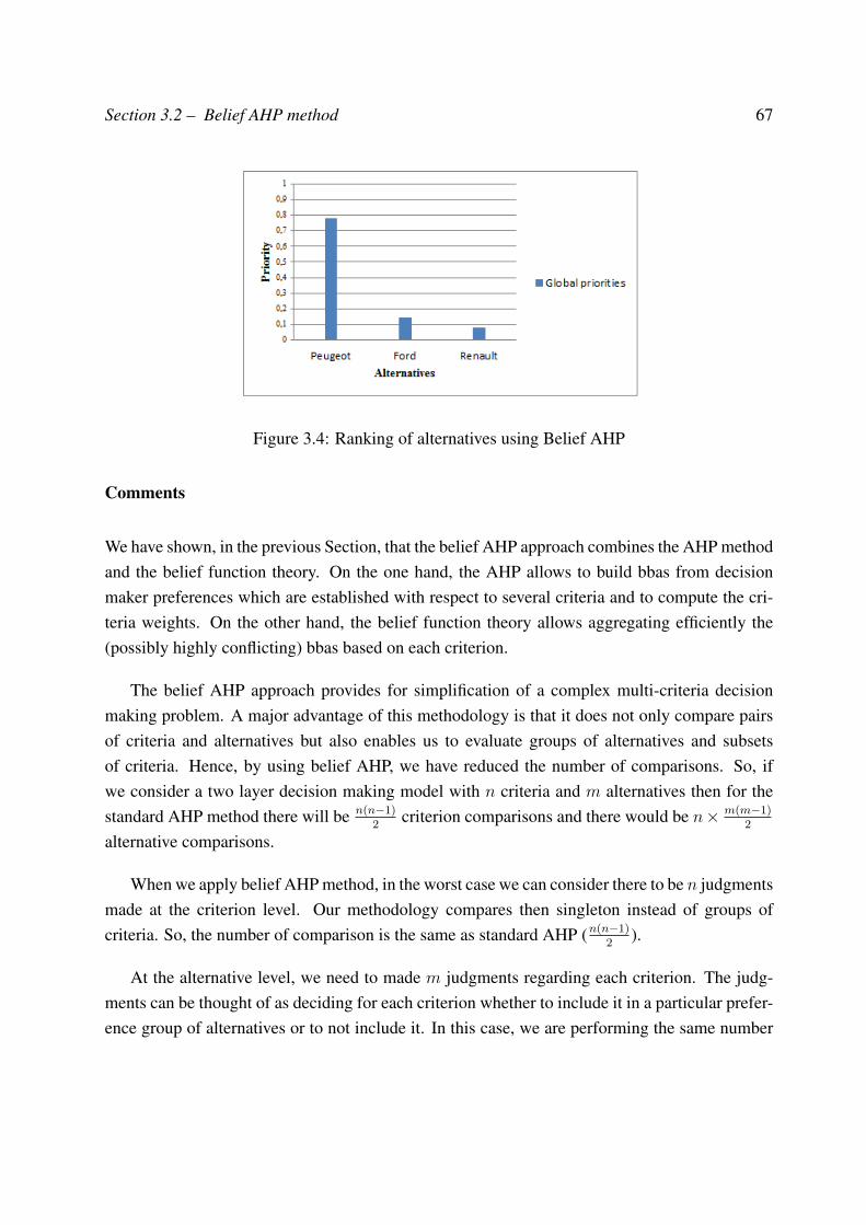
Section 3.2 – Belief AHP method 67
Figure 3.4: Ranking of alternatives using Belief AHP
Comments
We have shown, in the previous Section, that the belief AHP approach combines the AHP methodand the belief function theory. On the one hand, the AHP allows to build bbas from decisionmaker preferences which are established with respect to several criteria and to compute the cri-teria weights. On the other hand, the belief function theory allows aggregating efficiently the(possibly highly conflicting) bbas based on each criterion.
The belief AHP approach provides for simplification of a complex multi-criteria decisionmaking problem. A major advantage of this methodology is that it does not only compare pairsof criteria and alternatives but also enables us to evaluate groups of alternatives and subsetsof criteria. Hence, by using belief AHP, we have reduced the number of comparisons. So, ifwe consider a two layer decision making model with n criteria and m alternatives then for thestandard AHP method there will be n(n−1)
2criterion comparisons and there would be n× m(m−1)
2
alternative comparisons.
When we apply belief AHP method, in the worst case we can consider there to be n judgmentsmade at the criterion level. Our methodology compares then singleton instead of groups ofcriteria. So, the number of comparison is the same as standard AHP (n(n−1)
2).
At the alternative level, we need to made m judgments regarding each criterion. The judg-ments can be thought of as deciding for each criterion whether to include it in a particular prefer-ence group of alternatives or to not include it. In this case, we are performing the same number
Section 3.3 – A new belief AHP extension 68
of comparisons as DS/AHP method.
However, in the evaluation process, AHP assumes linear independence of criteria and alter-natives. It does not properly represent the evaluation of each alternative regarding each criterion.For instance, in a problem of buying a car, the expert might consider that Peugeot is evaluatedto be more important than Renault regarding Price criterion, but Renault is more important thanPeugeot with respect to Style criterion. As we can see, the alternative priorities are dependent oneach specific criterion. Hence, an extension of belief AHP method is proposed in order to modelthe dependency relation between alternatives and criteria.
3.3 A new belief AHP extension
In this Section, we develop a new AHP extension, called conditional belief AHP. Our approachtries to model a new relationship between alternatives and criteria.
3.3.1 Modeling dependency between alternatives and criteria
One of basic assumptions of AHP technique is that all the elements in the same hierarchy aretotally independent. However, this assumption is hard to be satisfied due to ambiguousness andcomplexity of questions. In addition to this problem, the evaluating elements include dependentproperties.
Under the AHP approach, criteria are assumed independent of the alternatives. However,paired comparisons imply dependence of a different kind. In fact, the importance assigned toan alternative depends on the evaluated criterion. This dependency is not according to structure,because we usually try to respect AHP axioms, but according to function.
In reality, when representing his assessments using the pair-wise comparison technique, thedecision maker expresses his preferences regarding the upper level. For instance, the alternativepriorities are usually dependent on each specific criterion. If the dependency among the elementsexists, it can distort the result significantly. So, to raise reliance of AHP, it is needed to considerthe effect of the degree of dependency between elements. In this study, we investigated thedependency and reflected that on belief AHP method.
Section 3.3 – A new belief AHP extension 69
Therefore, in the following Section, we propose a new AHP extension (Ennaceur et al.,2012b). Close to belief AHP, this model is called conditional belief AHP. Our aim throughthis work is then to represent uncertainty and to more imitate the expert reasoning, since he triesto express his preferences over the sets of alternatives regarding each criterion and not regardlessof the criteria. Consequently, we model the influences of the criteria on the evaluation of alter-natives. In making a decision, we need to allow for both and not to take the simple way out byalways assuming independency.
3.3.2 A new aggregation process using the belief function framework
In this part of this Chapter, we develop our second MCDM model named conditional beliefAHP. The difference between the two proposed methods is based on the aggregation procedure,as presented previously in Figure 3.1 (Step 3). Figure 3.5 summarizes the new computationalprocedure.
Figure 3.5: The general decision-making paradigm based on the conditional belief AHP
By introducing this approach, we try to model the relationship between alternatives and cri-teria. The developed method has the same steps as belief AHP. Nevertheless, we suggest a newaggregation procedure as shown in Figure 3.6.
After building the belief AHP hierarchy and completing the different pair-wise comparisonmatrices, we will be interested in this stage by showing how to combine the alternatives prioritieswith the importance of their corresponding criteria.

Section 3.3 – A new belief AHP extension 70
Figure 3.6: The new aggregation procedure under the conditional belief AHP method
Step 1: Representation of uncertainty
Through our approach, the uncertainty is introduced in the decision maker’s preferences. Be-sides, we propose to represent the imperfection over the sets of criteria. Within our framework,we have Ci ⊆ 2Ω and we have the priority values of each Ci representing the opinions-beliefs ofthe expert about his preferences. We also notice that this priority vector sums to one which canbe regarded as a bba. As a result, this bba can be denoted by mΩ.
Furthermore, we propose to represent the uncertainty at the level of alternatives. In fact,the expert tries to express his preferences regarding the sets of alternatives in relation with eachcriterion. Accordingly, and to more imitate the expert’s reasoning, we indicate that to define theinfluences of the criteria on the evaluation of alternatives, we might use a conditional belief.
Given a pair-wise comparison matrix which compares the sets of alternatives according to aspecific criterion, a conditional bba can be represented by:
mΘ[cj](Ak) = vk, ∀Ak ⊆ 2Θ and cj ∈ Ω . (3.9)
where Ak represents a subset of 2Θ, vk is the eigen value of the kth sets of alternatives regardingthe criterion cj . mΘ[cj](Ak) means that we know the belief about Ak regarding cj .
Example 3.5. Let us consider the same problem of purchasing a car (Example 3.1). We have fourcriteria: Ω = Price (c1), Style (c2), Fuel (c3), Reliability (c4) and three selected alternatives:Θ = Peugeot (p),Renault (r),Ford (f). The first step is to identify the subsets of criteria and the groups of alternatives asshown in the previous example. Then, we have to fill all the pair-wise comparison matrices andwe get the previous defined matrices (see Tables 3.1 and 3.3).
As indicated above, the criterion weights are expressed by a basic belief assessment (bba)
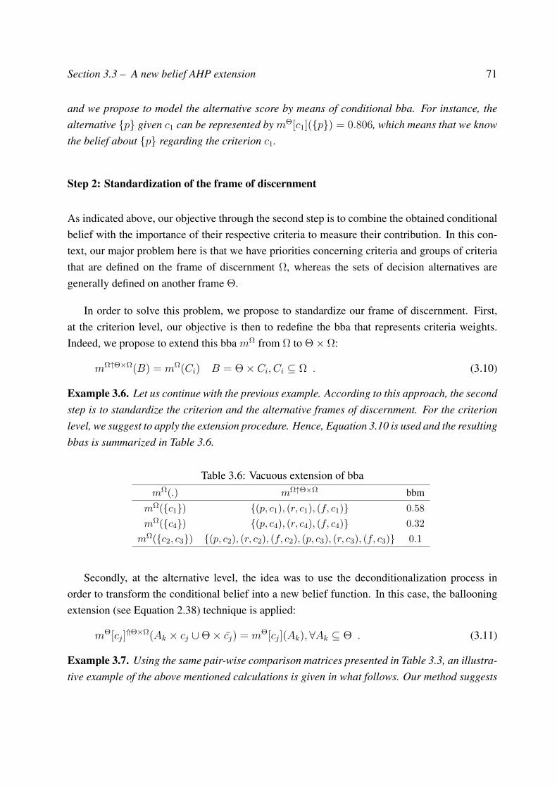
Section 3.3 – A new belief AHP extension 71
and we propose to model the alternative score by means of conditional bba. For instance, thealternative p given c1 can be represented by mΘ[c1](p) = 0.806, which means that we knowthe belief about p regarding the criterion c1.
Step 2: Standardization of the frame of discernment
As indicated above, our objective through the second step is to combine the obtained conditionalbelief with the importance of their respective criteria to measure their contribution. In this con-text, our major problem here is that we have priorities concerning criteria and groups of criteriathat are defined on the frame of discernment Ω, whereas the sets of decision alternatives aregenerally defined on another frame Θ.
In order to solve this problem, we propose to standardize our frame of discernment. First,at the criterion level, our objective is then to redefine the bba that represents criteria weights.Indeed, we propose to extend this bba mΩ from Ω to Θ× Ω:
mΩ↑Θ×Ω(B) = mΩ(Ci) B = Θ× Ci, Ci ⊆ Ω . (3.10)
Example 3.6. Let us continue with the previous example. According to this approach, the secondstep is to standardize the criterion and the alternative frames of discernment. For the criterionlevel, we suggest to apply the extension procedure. Hence, Equation 3.10 is used and the resultingbbas is summarized in Table 3.6.
Table 3.6: Vacuous extension of bbamΩ(.) mΩ↑Θ×Ω bbm
mΩ(c1) (p, c1), (r, c1), (f, c1) 0.58
mΩ(c4) (p, c4), (r, c4), (f, c4) 0.32
mΩ(c2, c3) (p, c2), (r, c2), (f, c2), (p, c3), (r, c3), (f, c3) 0.1
Secondly, at the alternative level, the idea was to use the deconditionalization process inorder to transform the conditional belief into a new belief function. In this case, the ballooningextension (see Equation 2.38) technique is applied:
mΘ[cj]⇑Θ×Ω(Ak × cj ∪Θ× cj) = mΘ[cj](Ak),∀Ak ⊆ Θ . (3.11)
Example 3.7. Using the same pair-wise comparison matrices presented in Table 3.3, an illustra-tive example of the above mentioned calculations is given in what follows. Our method suggests
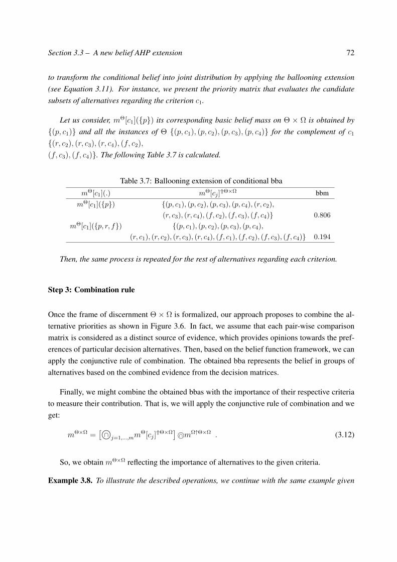
Section 3.3 – A new belief AHP extension 72
to transform the conditional belief into joint distribution by applying the ballooning extension(see Equation 3.11). For instance, we present the priority matrix that evaluates the candidatesubsets of alternatives regarding the criterion c1.
Let us consider, mΘ[c1](p) its corresponding basic belief mass on Θ × Ω is obtained by(p, c1) and all the instances of Θ (p, c1), (p, c2), (p, c3), (p, c4) for the complement of c1
(r, c2), (r, c3), (r, c4), (f, c2),
(f, c3), (f, c4). The following Table 3.7 is calculated.
Table 3.7: Ballooning extension of conditional bbamΘ[c1](.) mΘ[cj ]
⇑Θ×Ω bbm
mΘ[c1](p) (p, c1), (p, c2), (p, c3), (p, c4), (r, c2),
(r, c3), (r, c4), (f, c2), (f, c3), (f, c4) 0.806
mΘ[c1](p, r, f) (p, c1), (p, c2), (p, c3), (p, c4),
(r, c1), (r, c2), (r, c3), (r, c4), (f, c1), (f, c2), (f, c3), (f, c4) 0.194
Then, the same process is repeated for the rest of alternatives regarding each criterion.
Step 3: Combination rule
Once the frame of discernment Θ × Ω is formalized, our approach proposes to combine the al-ternative priorities as shown in Figure 3.6. In fact, we assume that each pair-wise comparisonmatrix is considered as a distinct source of evidence, which provides opinions towards the pref-erences of particular decision alternatives. Then, based on the belief function framework, we canapply the conjunctive rule of combination. The obtained bba represents the belief in groups ofalternatives based on the combined evidence from the decision matrices.
Finally, we might combine the obtained bbas with the importance of their respective criteriato measure their contribution. That is, we will apply the conjunctive rule of combination and weget:
mΘ×Ω =[∩©j=1,...,mm
Θ[cj]⇑Θ×Ω
]∩©mΩ↑Θ×Ω . (3.12)
So, we obtain mΘ×Ω reflecting the importance of alternatives to the given criteria.
Example 3.8. To illustrate the described operations, we continue with the same example given
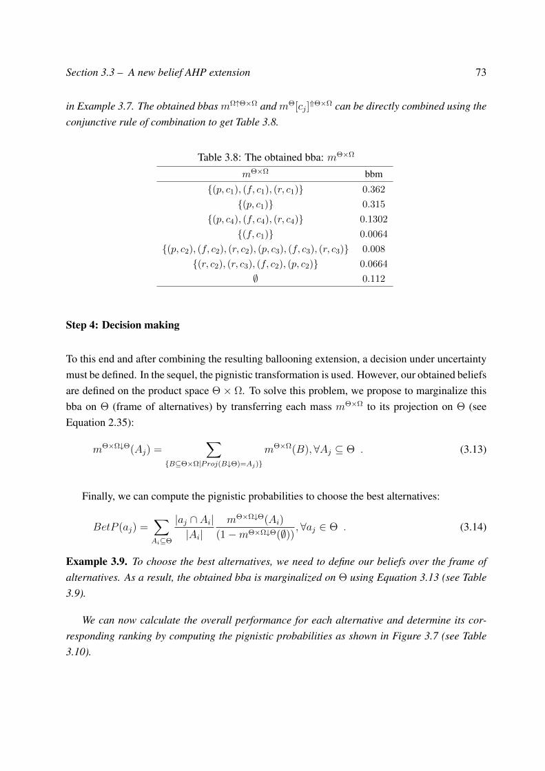
Section 3.3 – A new belief AHP extension 73
in Example 3.7. The obtained bbas mΩ↑Θ×Ω and mΘ[cj]⇑Θ×Ω can be directly combined using the
conjunctive rule of combination to get Table 3.8.
Table 3.8: The obtained bba: mΘ×Ω
mΘ×Ω bbm
(p, c1), (f, c1), (r, c1) 0.362
(p, c1) 0.315
(p, c4), (f, c4), (r, c4) 0.1302
(f, c1) 0.0064
(p, c2), (f, c2), (r, c2), (p, c3), (f, c3), (r, c3) 0.008
(r, c2), (r, c3), (f, c2), (p, c2) 0.0664
∅ 0.112
Step 4: Decision making
To this end and after combining the resulting ballooning extension, a decision under uncertaintymust be defined. In the sequel, the pignistic transformation is used. However, our obtained beliefsare defined on the product space Θ × Ω. To solve this problem, we propose to marginalize thisbba on Θ (frame of alternatives) by transferring each mass mΘ×Ω to its projection on Θ (seeEquation 2.35):
mΘ×Ω↓Θ(Aj) =∑
B⊆Θ×Ω|Proj(B↓Θ)=Aj)
mΘ×Ω(B),∀Aj ⊆ Θ . (3.13)
Finally, we can compute the pignistic probabilities to choose the best alternatives:
BetP (aj) =∑Ai⊆Θ
|aj ∩ Ai||Ai|
mΘ×Ω↓Θ(Ai)
(1−mΘ×Ω↓Θ(∅)),∀aj ∈ Θ . (3.14)
Example 3.9. To choose the best alternatives, we need to define our beliefs over the frame ofalternatives. As a result, the obtained bba is marginalized on Θ using Equation 3.13 (see Table3.9).
We can now calculate the overall performance for each alternative and determine its cor-responding ranking by computing the pignistic probabilities as shown in Figure 3.7 (see Table3.10).
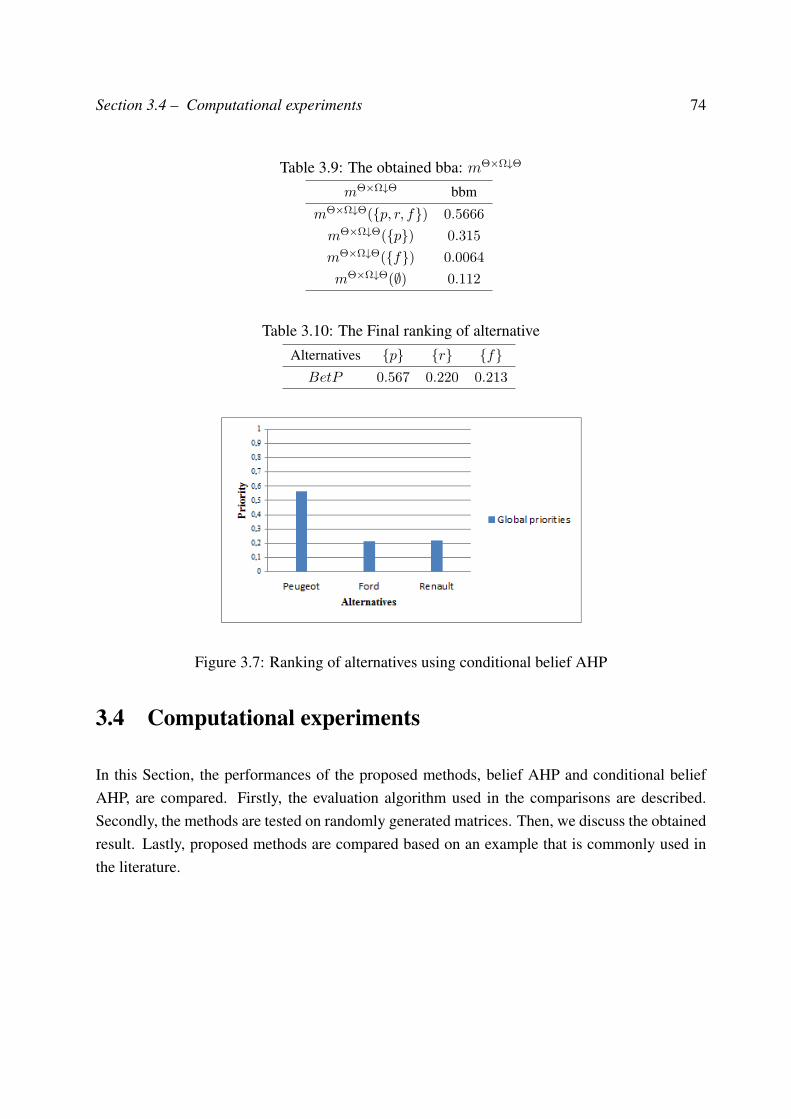
Section 3.4 – Computational experiments 74
Table 3.9: The obtained bba: mΘ×Ω↓Θ
mΘ×Ω↓Θ bbm
mΘ×Ω↓Θ(p, r, f) 0.5666
mΘ×Ω↓Θ(p) 0.315
mΘ×Ω↓Θ(f) 0.0064
mΘ×Ω↓Θ(∅) 0.112
Table 3.10: The Final ranking of alternativeAlternatives p r f
BetP 0.567 0.220 0.213
Figure 3.7: Ranking of alternatives using conditional belief AHP
3.4 Computational experiments
In this Section, the performances of the proposed methods, belief AHP and conditional beliefAHP, are compared. Firstly, the evaluation algorithm used in the comparisons are described.Secondly, the methods are tested on randomly generated matrices. Then, we discuss the obtainedresult. Lastly, proposed methods are compared based on an example that is commonly used inthe literature.
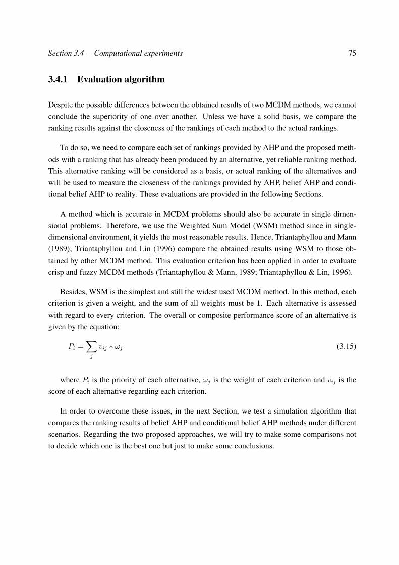
Section 3.4 – Computational experiments 75
3.4.1 Evaluation algorithm
Despite the possible differences between the obtained results of two MCDM methods, we cannotconclude the superiority of one over another. Unless we have a solid basis, we compare theranking results against the closeness of the rankings of each method to the actual rankings.
To do so, we need to compare each set of rankings provided by AHP and the proposed meth-ods with a ranking that has already been produced by an alternative, yet reliable ranking method.This alternative ranking will be considered as a basis, or actual ranking of the alternatives andwill be used to measure the closeness of the rankings provided by AHP, belief AHP and condi-tional belief AHP to reality. These evaluations are provided in the following Sections.
A method which is accurate in MCDM problems should also be accurate in single dimen-sional problems. Therefore, we use the Weighted Sum Model (WSM) method since in single-dimensional environment, it yields the most reasonable results. Hence, Triantaphyllou and Mann(1989); Triantaphyllou and Lin (1996) compare the obtained results using WSM to those ob-tained by other MCDM method. This evaluation criterion has been applied in order to evaluatecrisp and fuzzy MCDM methods (Triantaphyllou & Mann, 1989; Triantaphyllou & Lin, 1996).
Besides, WSM is the simplest and still the widest used MCDM method. In this method, eachcriterion is given a weight, and the sum of all weights must be 1. Each alternative is assessedwith regard to every criterion. The overall or composite performance score of an alternative isgiven by the equation:
Pi =∑j
vij ∗ ωj (3.15)
where Pi is the priority of each alternative, ωj is the weight of each criterion and vij is thescore of each alternative regarding each criterion.
In order to overcome these issues, in the next Section, we test a simulation algorithm thatcompares the ranking results of belief AHP and conditional belief AHP methods under differentscenarios. Regarding the two proposed approaches, we will try to make some comparisons notto decide which one is the best one but just to make some conclusions.
Section 3.4 – Computational experiments 76
3.4.2 Simulation algorithm
To generate reliable data for a numerical analysis in AHP, simulation has been extensively usedin prior research (Triantaphyllou & Lin, 1996; Triantaphyllou & Mann, 1989). The simulationalgorithm is summarized in Figure 3.8.
Figure 3.8: Simulation algorithm steps
The experiment is based on the following steps:
1. We generate a random matrix for the decision performance and another one to representthe weight of each decision criteria. Based on these two matrices, the overall scores andranks of the decision alternatives are calculated. These steps are usual steps in the WSMmethod.
2. From the performance matrix, we generated pair-wise comparison matrices of differentalternatives that are compared to each criterion.
3. We apply the suggested method to compute the overall priorities and to rank alternatives.
4. We compare the obtained result with the ranking of the WSM method.
Example 3.10. Let’s demonstrate the evaluation procedure using the same example used inTriantaphyllou and Mann (1989). We consider 3 alternatives a1, a2 and a3 and three criteria
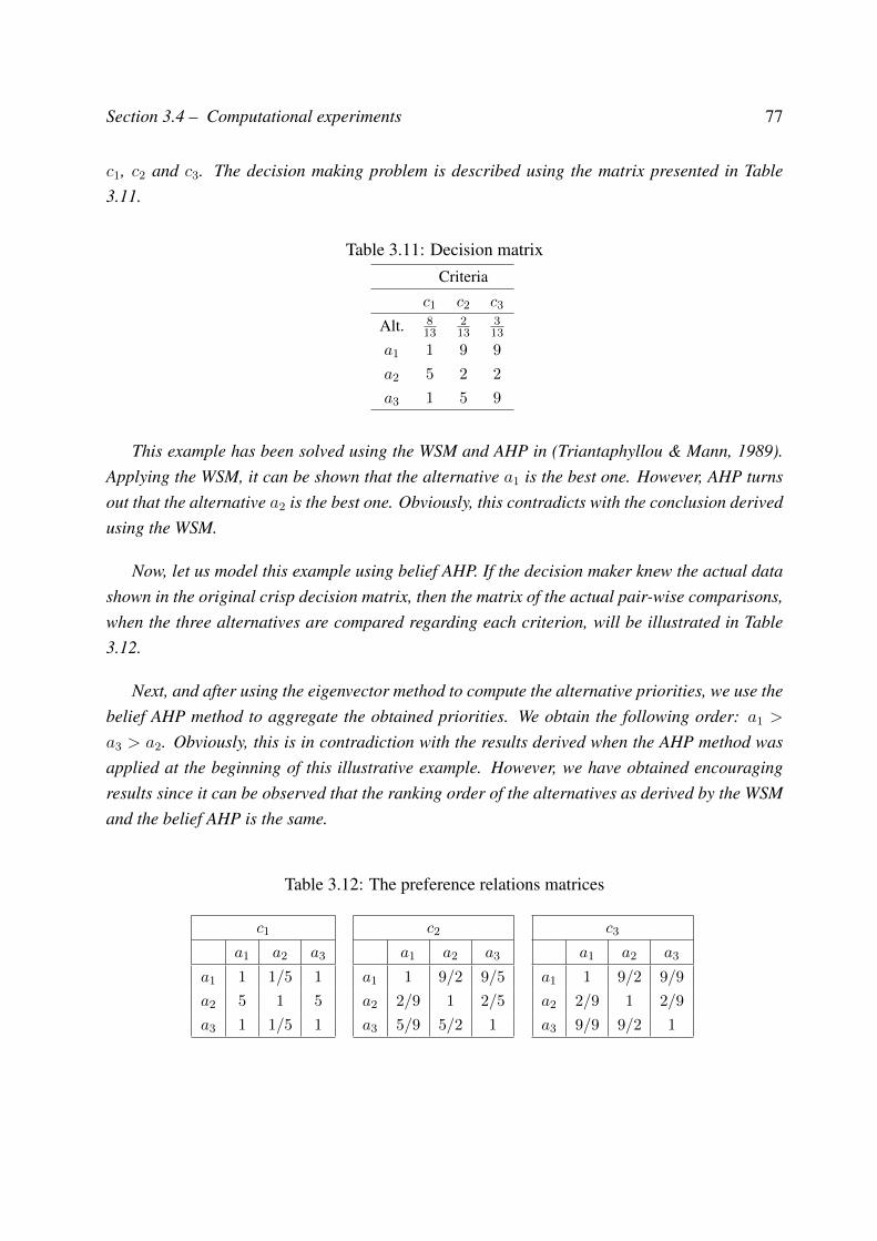
Section 3.4 – Computational experiments 77
c1, c2 and c3. The decision making problem is described using the matrix presented in Table3.11.
Table 3.11: Decision matrixCriteria
c1 c2 c3
Alt. 813
213
313
a1 1 9 9
a2 5 2 2
a3 1 5 9
This example has been solved using the WSM and AHP in (Triantaphyllou & Mann, 1989).Applying the WSM, it can be shown that the alternative a1 is the best one. However, AHP turnsout that the alternative a2 is the best one. Obviously, this contradicts with the conclusion derivedusing the WSM.
Now, let us model this example using belief AHP. If the decision maker knew the actual datashown in the original crisp decision matrix, then the matrix of the actual pair-wise comparisons,when the three alternatives are compared regarding each criterion, will be illustrated in Table3.12.
Next, and after using the eigenvector method to compute the alternative priorities, we use thebelief AHP method to aggregate the obtained priorities. We obtain the following order: a1 >
a3 > a2. Obviously, this is in contradiction with the results derived when the AHP method wasapplied at the beginning of this illustrative example. However, we have obtained encouragingresults since it can be observed that the ranking order of the alternatives as derived by the WSMand the belief AHP is the same.
Table 3.12: The preference relations matrices
c1
a1 a2 a3
a1 1 1/5 1
a2 5 1 5
a3 1 1/5 1
c2
a1 a2 a3
a1 1 9/2 9/5
a2 2/9 1 2/5
a3 5/9 5/2 1
c3
a1 a2 a3
a1 1 9/2 9/9
a2 2/9 1 2/9
a3 9/9 9/2 1
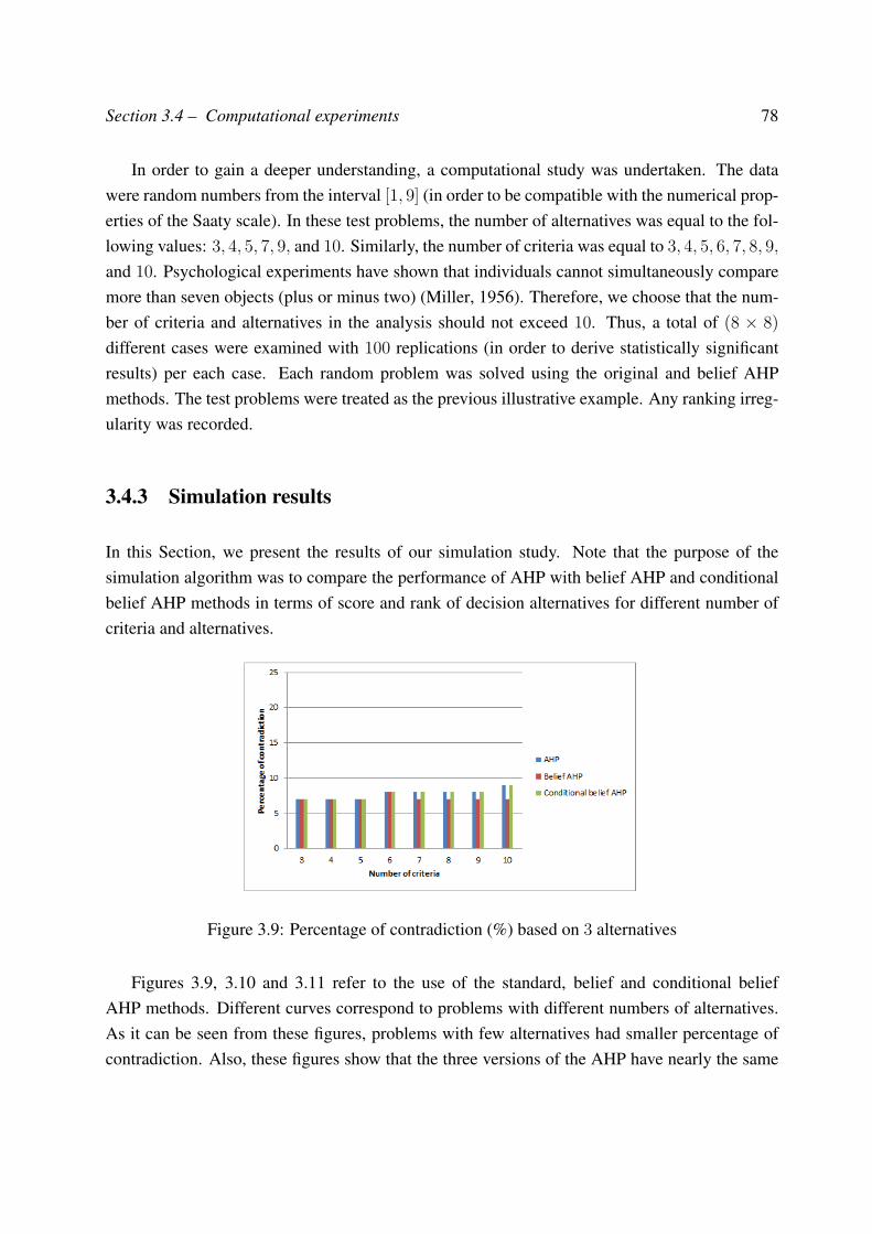
Section 3.4 – Computational experiments 78
In order to gain a deeper understanding, a computational study was undertaken. The datawere random numbers from the interval [1, 9] (in order to be compatible with the numerical prop-erties of the Saaty scale). In these test problems, the number of alternatives was equal to the fol-lowing values: 3, 4, 5, 7, 9, and 10. Similarly, the number of criteria was equal to 3, 4, 5, 6, 7, 8, 9,
and 10. Psychological experiments have shown that individuals cannot simultaneously comparemore than seven objects (plus or minus two) (Miller, 1956). Therefore, we choose that the num-ber of criteria and alternatives in the analysis should not exceed 10. Thus, a total of (8 × 8)
different cases were examined with 100 replications (in order to derive statistically significantresults) per each case. Each random problem was solved using the original and belief AHPmethods. The test problems were treated as the previous illustrative example. Any ranking irreg-ularity was recorded.
3.4.3 Simulation results
In this Section, we present the results of our simulation study. Note that the purpose of thesimulation algorithm was to compare the performance of AHP with belief AHP and conditionalbelief AHP methods in terms of score and rank of decision alternatives for different number ofcriteria and alternatives.
Figure 3.9: Percentage of contradiction (%) based on 3 alternatives
Figures 3.9, 3.10 and 3.11 refer to the use of the standard, belief and conditional beliefAHP methods. Different curves correspond to problems with different numbers of alternatives.As it can be seen from these figures, problems with few alternatives had smaller percentage ofcontradiction. Also, these figures show that the three versions of the AHP have nearly the same
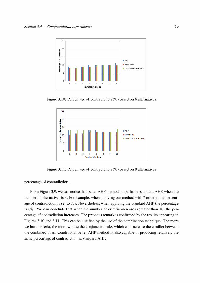
Section 3.4 – Computational experiments 79
Figure 3.10: Percentage of contradiction (%) based on 6 alternatives
Figure 3.11: Percentage of contradiction (%) based on 9 alternatives
percentage of contradiction.
From Figure 3.9, we can notice that belief AHP method outperforms standard AHP, when thenumber of alternatives is 3. For example, when applying our method with 7 criteria, the percent-age of contradiction is set to 7%. Nevertheless, when applying the standard AHP the percentageis 8%. We can conclude that when the number of criteria increases (greater than 10) the per-centage of contradiction increases. The previous remark is confirmed by the results appearing inFigures 3.10 and 3.11. This can be justified by the use of the combination technique. The morewe have criteria, the more we use the conjunctive rule, which can increase the conflict betweenthe combined bbas. Conditional belief AHP method is also capable of producing relatively thesame percentage of contradiction as standard AHP.
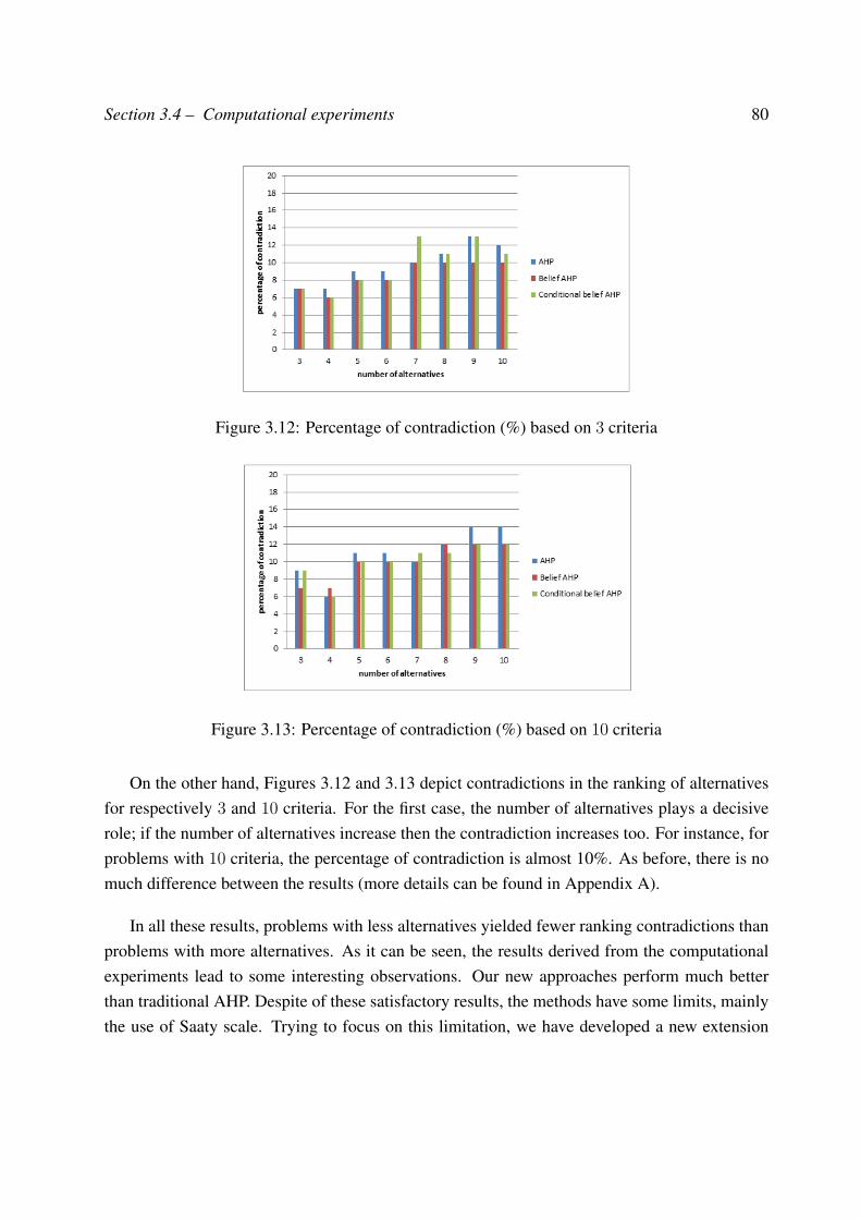
Section 3.4 – Computational experiments 80
Figure 3.12: Percentage of contradiction (%) based on 3 criteria
Figure 3.13: Percentage of contradiction (%) based on 10 criteria
On the other hand, Figures 3.12 and 3.13 depict contradictions in the ranking of alternativesfor respectively 3 and 10 criteria. For the first case, the number of alternatives plays a decisiverole; if the number of alternatives increase then the contradiction increases too. For instance, forproblems with 10 criteria, the percentage of contradiction is almost 10%. As before, there is nomuch difference between the results (more details can be found in Appendix A).
In all these results, problems with less alternatives yielded fewer ranking contradictions thanproblems with more alternatives. As it can be seen, the results derived from the computationalexperiments lead to some interesting observations. Our new approaches perform much betterthan traditional AHP. Despite of these satisfactory results, the methods have some limits, mainlythe use of Saaty scale. Trying to focus on this limitation, we have developed a new extension
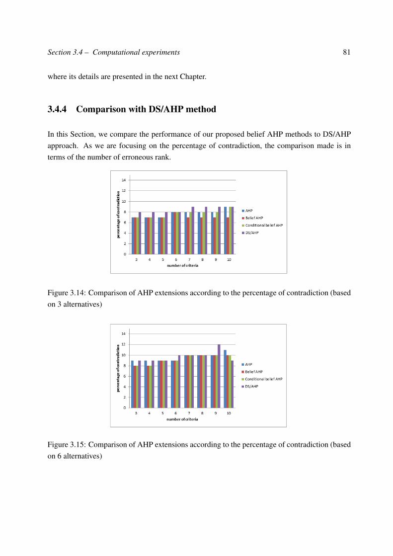
Section 3.4 – Computational experiments 81
where its details are presented in the next Chapter.
3.4.4 Comparison with DS/AHP method
In this Section, we compare the performance of our proposed belief AHP methods to DS/AHPapproach. As we are focusing on the percentage of contradiction, the comparison made is interms of the number of erroneous rank.
Figure 3.14: Comparison of AHP extensions according to the percentage of contradiction (basedon 3 alternatives)
Figure 3.15: Comparison of AHP extensions according to the percentage of contradiction (basedon 6 alternatives)
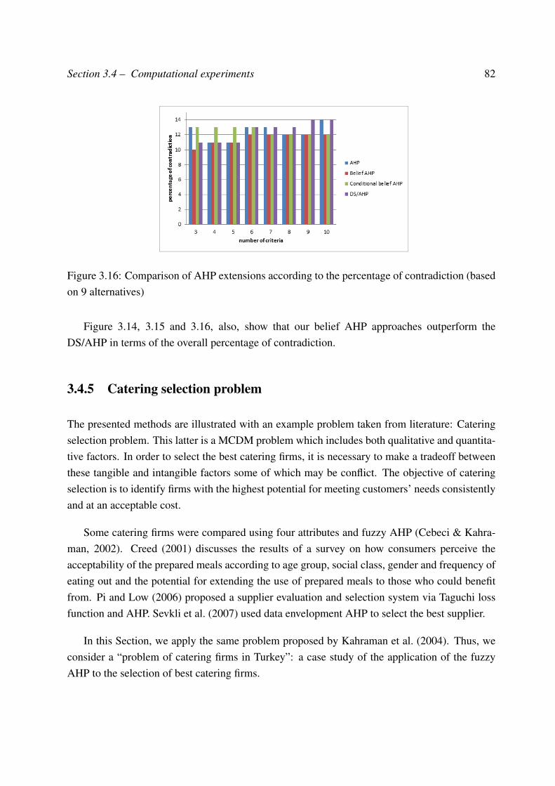
Section 3.4 – Computational experiments 82
Figure 3.16: Comparison of AHP extensions according to the percentage of contradiction (basedon 9 alternatives)
Figure 3.14, 3.15 and 3.16, also, show that our belief AHP approaches outperform theDS/AHP in terms of the overall percentage of contradiction.
3.4.5 Catering selection problem
The presented methods are illustrated with an example problem taken from literature: Cateringselection problem. This latter is a MCDM problem which includes both qualitative and quantita-tive factors. In order to select the best catering firms, it is necessary to make a tradeoff betweenthese tangible and intangible factors some of which may be conflict. The objective of cateringselection is to identify firms with the highest potential for meeting customers’ needs consistentlyand at an acceptable cost.
Some catering firms were compared using four attributes and fuzzy AHP (Cebeci & Kahra-man, 2002). Creed (2001) discusses the results of a survey on how consumers perceive theacceptability of the prepared meals according to age group, social class, gender and frequency ofeating out and the potential for extending the use of prepared meals to those who could benefitfrom. Pi and Low (2006) proposed a supplier evaluation and selection system via Taguchi lossfunction and AHP. Sevkli et al. (2007) used data envelopment AHP to select the best supplier.
In this Section, we apply the same problem proposed by Kahraman et al. (2004). Thus, weconsider a “problem of catering firms in Turkey”: a case study of the application of the fuzzyAHP to the selection of best catering firms.
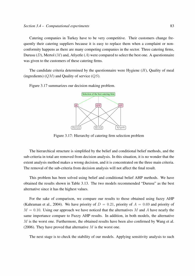
Section 3.4 – Computational experiments 83
Catering companies in Turkey have to be very competitive. Their customers change fre-quently their catering suppliers because it is easy to replace them when a complaint or non-conformity happens as there are many competing companies in the sector. Three catering firms,Durusu (D), Mertol (M ) and, Afiyetle (A) were compared to select the best one. A questionnairewas given to the customers of these catering firms.
The candidate criteria determined by the questionnaire were Hygiene (H), Quality of meal(ingredients) (QM ) and Quality of service (QS).
Figure 3.17 summarizes our decision making problem.
Selection of the best catering firm
H QM QS
Durusu Mertol Afiyetle
Figure 3.17: Hierarchy of catering firm selection problem
The hierarchical structure is simplified by the belief and conditional belief methods, and thesub-criteria in total are removed from decision analysis. In this situation, it is no wonder that theextent analysis method makes a wrong decision, and it is concentrated on the three main criteria.The removal of the sub-criteria from decision analysis will not affect the final result.
This problem has been solved using belief and conditional belief AHP methods. We haveobtained the results shown in Table 3.13. The two models recommended “Durusu” as the bestalternative since it has the highest values.
For the sake of comparison, we compare our results to those obtained using fuzzy AHP(Kahraman et al., 2004). We have priority of D = 0.21, priority of A = 0.69 and priority ofM = 0.10. Using our approach we have noticed that the alternatives M and A have nearly thesame importance compare to Fuzzy AHP results. In addition, in both models, the alternativeM is the worst one. Furthermore, the obtained results have been also confirmed by Wang et al.(2006). They have proved that alternative M is the worst one.
The next stage is to check the stability of our models. Applying sensitivity analysis to such
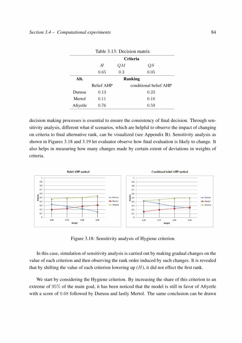
Section 3.4 – Computational experiments 84
Table 3.13: Decision matrixCriteria
H QM QS
0.65 0.3 0.05
Alt. RankingBelief AHP conditional belief AHP
Durusu 0.13 0.23
Mertol 0.11 0.18
Afiyetle 0.76 0.59
decision making processes is essential to ensure the consistency of final decision. Through sen-sitivity analysis, different what-if scenarios, which are helpful to observe the impact of changingon criteria to final alternative rank, can be visualized (see Appendix B). Sensitivity analysis asshown in Figures 3.18 and 3.19 let evaluator observe how final evaluation is likely to change. Italso helps in measuring how many changes made by certain extent of deviations in weights ofcriteria.
Figure 3.18: Sensitivity analysis of Hygiene criterion
In this case, simulation of sensitivity analysis is carried out by making gradual changes on thevalue of each criterion and then observing the rank order induced by such changes. It is revealedthat by shifting the value of each criterion lowering up (H), it did not effect the first rank.
We start by considering the Hygiene criterion. By increasing the share of this criterion to anextreme of 95% of the main goal, it has been noticed that the model is still in favor of Afiyetlewith a score of 0.68 followed by Durusu and lastly Mertol. The same conclusion can be drawn
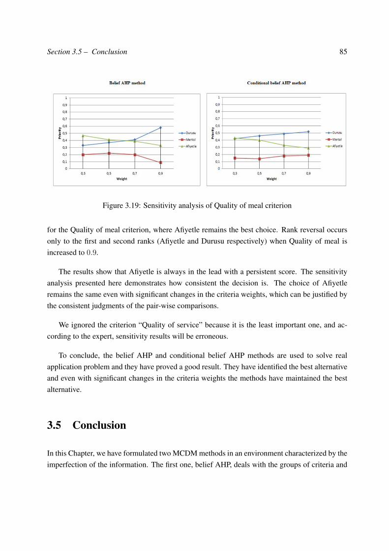
Section 3.5 – Conclusion 85
Figure 3.19: Sensitivity analysis of Quality of meal criterion
for the Quality of meal criterion, where Afiyetle remains the best choice. Rank reversal occursonly to the first and second ranks (Afiyetle and Durusu respectively) when Quality of meal isincreased to 0.9.
The results show that Afiyetle is always in the lead with a persistent score. The sensitivityanalysis presented here demonstrates how consistent the decision is. The choice of Afiyetleremains the same even with significant changes in the criteria weights, which can be justified bythe consistent judgments of the pair-wise comparisons.
We ignored the criterion “Quality of service” because it is the least important one, and ac-cording to the expert, sensitivity results will be erroneous.
To conclude, the belief AHP and conditional belief AHP methods are used to solve realapplication problem and they have proved a good result. They have identified the best alternativeand even with significant changes in the criteria weights the methods have maintained the bestalternative.
3.5 Conclusion
In this Chapter, we have formulated two MCDM methods in an environment characterized by theimperfection of the information. The first one, belief AHP, deals with the groups of criteria and
Section 3.5 – Conclusion 86
alternatives. Then, an extension of this approach, named conditional belief AHP, is introduced.It takes into account the dependency relationships between criteria and alternatives.
The belief AHP approaches proved to be a convenient method in tackling practical MCDMproblems. They were used to synthesize the opinions of the decision maker to reduce the numberof comparisons. They show the advantage of being able to imitate human thinking and aid insolving the research problem through modeling dependency between alternatives and criteria.The two proposed methods have been illustrated by a simple example. Then, we have comparedthem through random problems. Finally, we have used them to solve a problem from literature.
Nevertheless, these methods assume that a decision maker can provide precise point estimatesof his preferences. Hence, Saaty scale is not suitable for scenarios when there is high uncertaintyin decision makers judgment.
To overcome this limitation, belief AHP approaches will serve as a base to the proposedmethods that will be introduced in the following Chapter. A new preference elicitation technique,which incorporates belief distributions to include uncertainty in the judgments, will be suggested.
Chapter 4A new ranking procedure by beliefpair-wise comparisons
4.1 Introduction
Despite its popularity and efficiency, the AHP method is often criticized for its use of an un-balanced scale of estimations and its inability to adequately handle the uncertainty associatedwith the mapping of the decision maker’s perception to a crisp number. Besides, in MCDM pro-cess, an expert may be uncertain about his level of preference due to incomplete information orknowledge, inherent complexity and uncertainty within the decision environment.
Therefore, our main aim through this research is to extend the pair-wise comparison processon a more flexible method that integrates additional uncertain and/or imprecise knowledge. Anatural way to cope with uncertain judgments is to express the comparison ratios as a belieffunction, which incorporates the imperfection of the human thinking. Thus, a new procedure isemployed to derive crisp priorities from belief distributions based on a new set of choices.
In this Chapter, we give an insight into our proposed methods. We first present, in Section4.2, some motivations to develop the belief pair-wise comparison. Next, Section 4.3 details ournew belief pair-wise comparisons along with examples to illustrate them. Then, we introduce, inSection 4.4, our proposed MCDM methodology based on belief pair-wise comparison. Section4.5 models dependency between alternatives and criteria under Yes-No/AHP framework. In the
87
Section 4.2 – Limits of Saaty scale 88
last Section (Section 4.6), we present some experimental studies.
4.2 Limits of Saaty scale
In MCDM, the pair-wise comparisons represent a useful starting point for determining a rankingon a set of alternatives or criteria. It aims at quantifying relative priorities for a given set ofalternatives as well as the set of criteria, on a ratio scale, based on the judgment of the decisionmaker.
The scale used in the AHP for pair-wise comparisons is the 1 to 9 ratio scale (Saaty, 1977,1980). We note that the inverse relationships are simply the multiplicative inverses of the valuesfrom within the 1 to 9 scale, hence the actual scale used in the AHP is 1/9 to 1 to 9.
Using this approach, the decision maker has to express his opinion about the value of onesingle pair-wise comparison at a time. Usually, he has to choose his answer among discretechoices. Each choice is a linguistic phrase. Some examples of such linguistic phrases are: “A ismore important than B”, or “A is of the same importance as B”, or “A is a little more importantthan B”, and so on. He uses Saaty’s scale (see Table 1.4) to map the labels which indicate thedecision maker view to a numeric value.
However, as shown in Joaquin (1990) and Holder (1995), this scale was criticized since theuser cannot be consistent. Sometimes, the decision maker may well want to say that A is twiceas important as B, A is 3 times as important as C and B is 1.5 times as important as C, yet he isconstrained to make the last judgment 1 or 2. In addition, the decision maker might find difficultto distinguish among them and tell for example whether one alternative is 6 or 7 times moreimportant than another. Furthermore, the AHP method cannot cope with the fact that alternativeA is 25 times more important than alternative C. Expert would not be able to efficiently expressany kind of preference degree between the available alternatives and criteria. As a result, thescale is further incomplete and unnecessarily restricting because of the arbitrary cut-off at 9 forthe maximum allowable ratio of weights.
All these criticisms have been discussed in the literature and some solutions for them havebeen developed. To take judgmental uncertainty into account, alternative methods such as ap-plications of the fuzzy theory are developed for AHP (Laarhoven & Pedrycz, 1983; Lootsma,1997). Different scaling methods have also been provided (Beynon, 2002a).

Section 4.3 – A pair-wise comparison process: A new elicitation technique 89
Consequently, our problem through this work is: how to quantify the linguistic choices se-lected by the decision maker during the evaluation of the pair-wise comparisons under the belieffunction framework? Is it necessary to decompose even more the different levels of the Saaty’sscale?
4.3 A pair-wise comparison process: A new elicitation tech-nique
Since using belief distribution as an element of the pair-wise comparison matrix is more ex-pressive than using crisp number, we expect that belief approach allows for a more accuratedescription of the decision making process. Rather than forcing the expert to provide exact rep-resentations of imprecise perceptions, we suggest using an imprecise representation instead.
In this Section, we suggest to modify the structure of the Saaty scale by adopting a new setof choices. We present the definitions and notations for the pair-wise comparison matrix. Then,the inconsistency identification method is introduced.
4.3.1 Pair-wise comparison matrix with belief distributions
Under this approach, a new elicitation procedure is introduced. Thus to model his assessments,the decision maker has to express his opinions qualitatively. He indicates whether a criterion (oralternative) was more or less important to its partner. Therefore, we suggest a new set of choices.For instance, to respond to the following question: “Is the subset of criteria Cj important?”, theexpert only selects the related linguistic variable. He indicated whether a criterion was more orless important by “yes” or “no”. In other terms:
ΩCj= yes, no (4.1)
where ΩCjis the set of possible choices.
Moreover, we accept that the expert may define uncertain or even unknown assessments. In-deed, we assume that each subset of criteria is described by a basic belief assignment definedon the possible responses (mΩCj ). In other words, to quantify the subjective judgments with un-certainty, a preference degree may be assigned to each decision maker’s response. For instance,
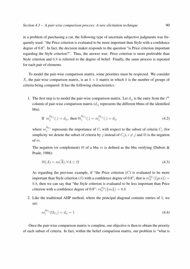
Section 4.3 – A pair-wise comparison process: A new elicitation technique 90
in a problem of purchasing a car, the following type of uncertain subjective judgments was fre-quently used: “the Price criterion is evaluated to be more important than Style with a confidencedegree of 0.8”. In fact, the decision maker responds to the question “is Price criterion importantregarding the Style criterion?”. Thus, the answer was: Price criterion is more preferable thanStyle criterion and 0.8 is referred to the degree of belief. Finally, the same process is repeatedfor each pair of elements.
To model the pair-wise comparison matrix, some priorities must be respected. We considerX , the pair-wise comparison matrix, is an k × k matrix in which k is the number of groups ofcriteria being compared. It has the following characteristics:
1. The first step is to model the pair-wise comparison matrix. Let dij is the entry from the ith
column of pair-wise comparison matrix (dij represents the different bbms of the identifiedbba).
If mΩCij (.) = dij, then m
ΩCj
i (.) = mΩCij (.) = dij (4.2)
where mΩCij represents the importance of Ci with respect to the subset of criteria Cj (for
simplicity we denote the subset of criteria by j instead of Cj), i 6= j and m is the negationof m.
The negation (or complement) m of a bba m is defined as the bba verifying (Dubois &Prade, 1986):
m(A) = m(A), ∀A ⊂ Ω (4.3)
As regarding the previous example, if “the Price criterion (C) is evaluated to be moreimportant than Style criterion (S) with a confidence degree of 0.8”, that is mΩC
S (yes) =
0.8, then we can say that “the Style criterion is evaluated to be less important than Pricecriterion with a confidence degree of 0.8”: mΩS
C (no) = 0.8.
2. Like the traditional AHP method, where the principal diagonal contains entries of 1, weset:
mΩCii (ΩCi
) = dii = 1 (4.4)
Once the pair-wise comparison matrix is complete, our objective is then to obtain the priorityof each subset of criteria. In fact, within the belief comparison matrix, our problem is “what is
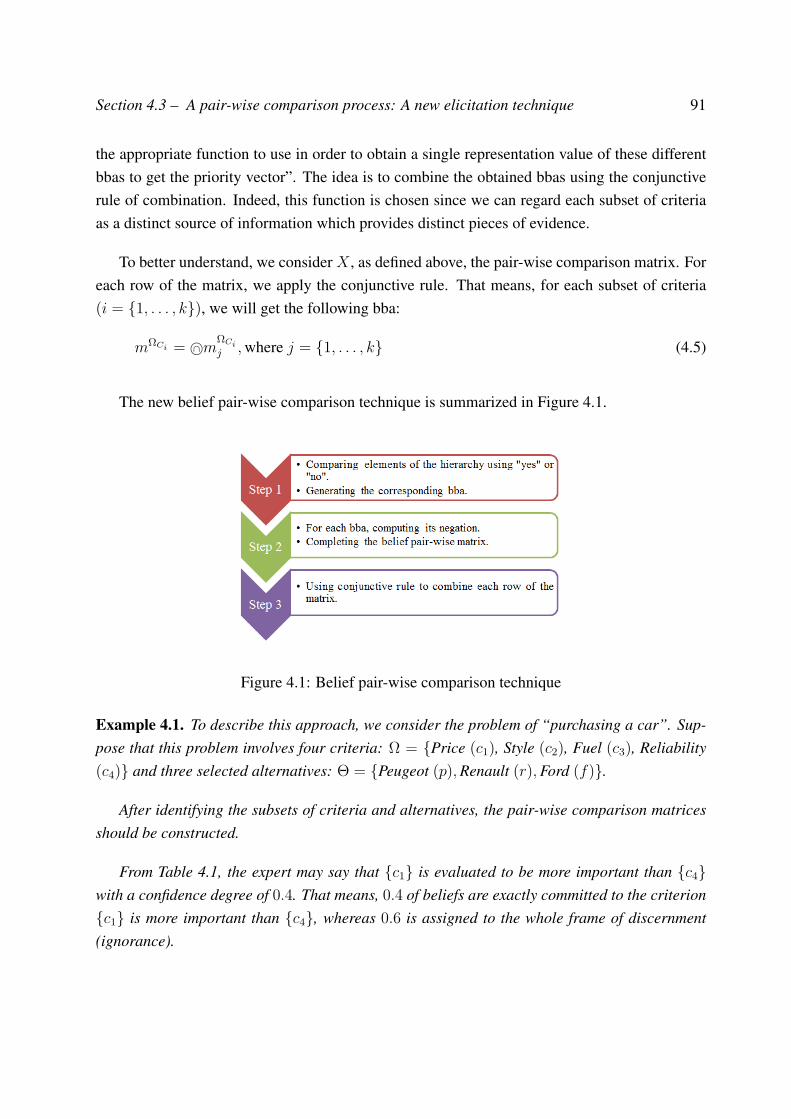
Section 4.3 – A pair-wise comparison process: A new elicitation technique 91
the appropriate function to use in order to obtain a single representation value of these differentbbas to get the priority vector”. The idea is to combine the obtained bbas using the conjunctiverule of combination. Indeed, this function is chosen since we can regard each subset of criteriaas a distinct source of information which provides distinct pieces of evidence.
To better understand, we consider X , as defined above, the pair-wise comparison matrix. Foreach row of the matrix, we apply the conjunctive rule. That means, for each subset of criteria(i = 1, . . . , k), we will get the following bba:
mΩCi = ∩©mΩCij ,where j = 1, . . . , k (4.5)
The new belief pair-wise comparison technique is summarized in Figure 4.1.
Figure 4.1: Belief pair-wise comparison technique
Example 4.1. To describe this approach, we consider the problem of “purchasing a car”. Sup-pose that this problem involves four criteria: Ω = Price (c1), Style (c2), Fuel (c3), Reliability(c4) and three selected alternatives: Θ = Peugeot (p),Renault (r),Ford (f).
After identifying the subsets of criteria and alternatives, the pair-wise comparison matricesshould be constructed.
From Table 4.1, the expert may say that c1 is evaluated to be more important than c4with a confidence degree of 0.4. That means, 0.4 of beliefs are exactly committed to the criterionc1 is more important than c4, whereas 0.6 is assigned to the whole frame of discernment(ignorance).
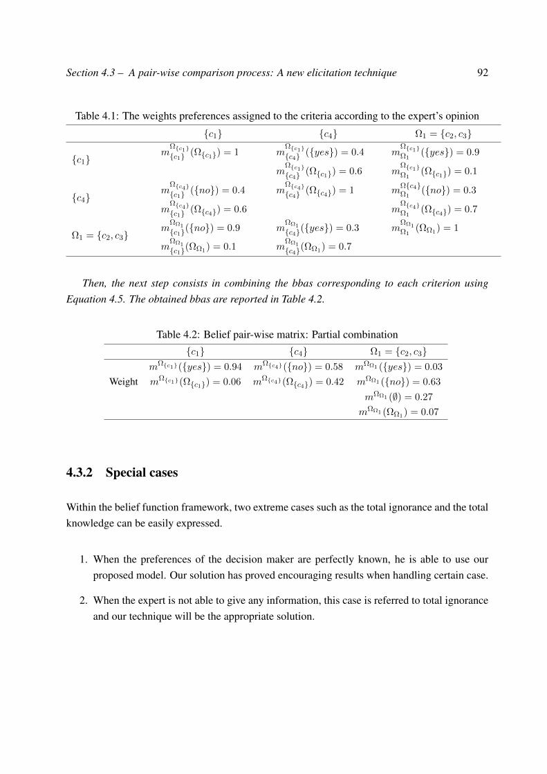
Section 4.3 – A pair-wise comparison process: A new elicitation technique 92
Table 4.1: The weights preferences assigned to the criteria according to the expert’s opinion
c1 c4 Ω1 = c2, c3
c1m
Ωc1c1 (Ωc1) = 1 m
Ωc1c4 (yes) = 0.4 m
Ωc1Ω1
(yes) = 0.9
mΩc1c4 (Ωc1) = 0.6 m
Ωc1Ω1
(Ωc1) = 0.1
c4m
Ωc4c1 (no) = 0.4 m
Ωc4c4 (Ωc4) = 1 m
Ωc4Ω1
(no) = 0.3
mΩc4c1 (Ωc4) = 0.6 m
Ωc4Ω1
(Ωc4) = 0.7
Ω1 = c2, c3m
ΩΩ1
c1(no) = 0.9 mΩΩ1
c4(yes) = 0.3 mΩΩ1Ω1
(ΩΩ1) = 1
mΩΩ1
c1(ΩΩ1) = 0.1 mΩΩ1
c4(ΩΩ1) = 0.7
Then, the next step consists in combining the bbas corresponding to each criterion usingEquation 4.5. The obtained bbas are reported in Table 4.2.
Table 4.2: Belief pair-wise matrix: Partial combinationc1 c4 Ω1 = c2, c3
WeightmΩc1(yes) = 0.94 mΩc4(no) = 0.58 mΩΩ1 (yes) = 0.03
mΩc1(Ωc1) = 0.06 mΩc4(Ωc4) = 0.42 mΩΩ1 (no) = 0.63
mΩΩ1 (∅) = 0.27
mΩΩ1 (ΩΩ1) = 0.07
4.3.2 Special cases
Within the belief function framework, two extreme cases such as the total ignorance and the totalknowledge can be easily expressed.
1. When the preferences of the decision maker are perfectly known, he is able to use ourproposed model. Our solution has proved encouraging results when handling certain case.
2. When the expert is not able to give any information, this case is referred to total ignoranceand our technique will be the appropriate solution.
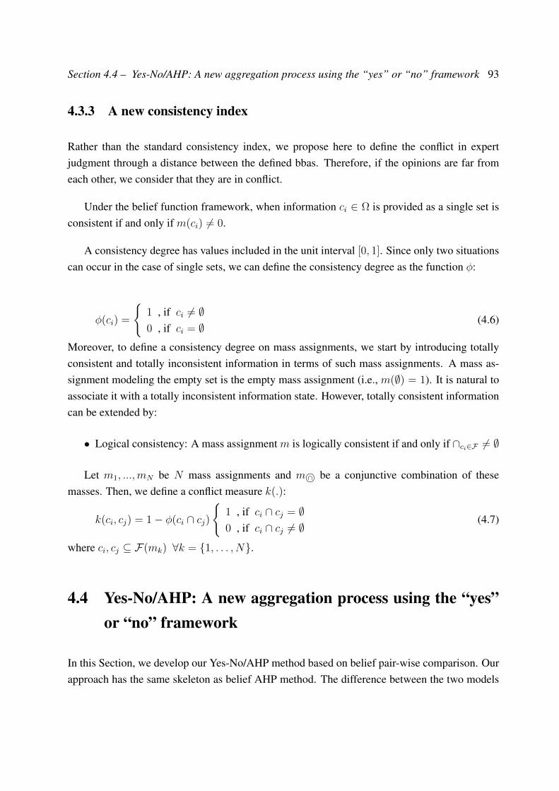
Section 4.4 – Yes-No/AHP: A new aggregation process using the “yes” or “no” framework 93
4.3.3 A new consistency index
Rather than the standard consistency index, we propose here to define the conflict in expertjudgment through a distance between the defined bbas. Therefore, if the opinions are far fromeach other, we consider that they are in conflict.
Under the belief function framework, when information ci ∈ Ω is provided as a single set isconsistent if and only if m(ci) 6= 0.
A consistency degree has values included in the unit interval [0, 1]. Since only two situationscan occur in the case of single sets, we can define the consistency degree as the function φ:
φ(ci) =
1 , if ci 6= ∅0 , if ci = ∅
(4.6)
Moreover, to define a consistency degree on mass assignments, we start by introducing totallyconsistent and totally inconsistent information in terms of such mass assignments. A mass as-signment modeling the empty set is the empty mass assignment (i.e., m(∅) = 1). It is natural toassociate it with a totally inconsistent information state. However, totally consistent informationcan be extended by:
• Logical consistency: A mass assignment m is logically consistent if and only if ∩ci∈F 6= ∅
Let m1, ...,mN be N mass assignments and m ∩© be a conjunctive combination of thesemasses. Then, we define a conflict measure k(.):
k(ci, cj) = 1− φ(ci ∩ cj)
1 , if ci ∩ cj = ∅0 , if ci ∩ cj 6= ∅
(4.7)
where ci, cj ⊆ F(mk) ∀k = 1, . . . , N.
4.4 Yes-No/AHP: A new aggregation process using the “yes”or “no” framework
In this Section, we develop our Yes-No/AHP method based on belief pair-wise comparison. Ourapproach has the same skeleton as belief AHP method. The difference between the two models
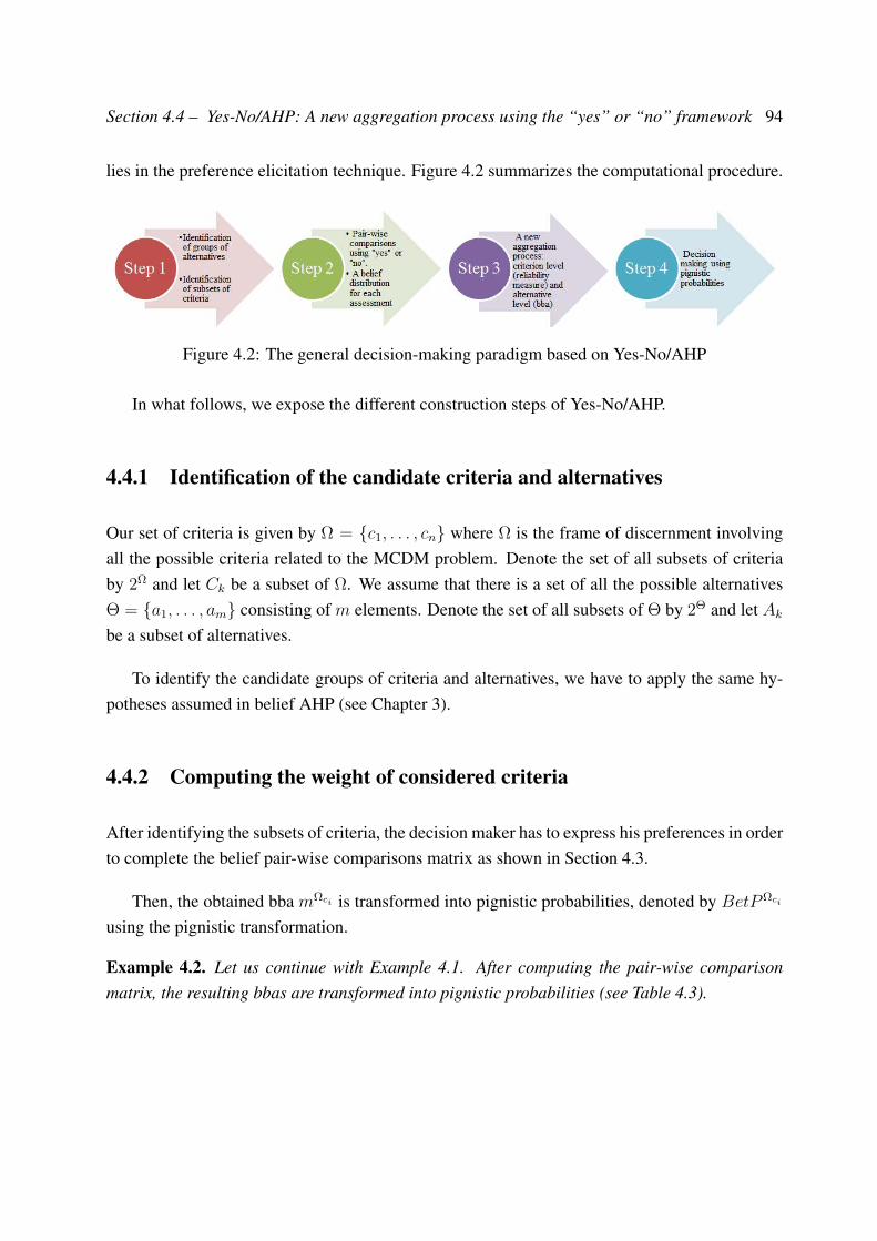
Section 4.4 – Yes-No/AHP: A new aggregation process using the “yes” or “no” framework 94
lies in the preference elicitation technique. Figure 4.2 summarizes the computational procedure.
Figure 4.2: The general decision-making paradigm based on Yes-No/AHP
In what follows, we expose the different construction steps of Yes-No/AHP.
4.4.1 Identification of the candidate criteria and alternatives
Our set of criteria is given by Ω = c1, . . . , cn where Ω is the frame of discernment involvingall the possible criteria related to the MCDM problem. Denote the set of all subsets of criteriaby 2Ω and let Ck be a subset of Ω. We assume that there is a set of all the possible alternativesΘ = a1, . . . , am consisting of m elements. Denote the set of all subsets of Θ by 2Θ and let Ak
be a subset of alternatives.
To identify the candidate groups of criteria and alternatives, we have to apply the same hy-potheses assumed in belief AHP (see Chapter 3).
4.4.2 Computing the weight of considered criteria
After identifying the subsets of criteria, the decision maker has to express his preferences in orderto complete the belief pair-wise comparisons matrix as shown in Section 4.3.
Then, the obtained bba mΩci is transformed into pignistic probabilities, denoted by BetPΩci
using the pignistic transformation.
Example 4.2. Let us continue with Example 4.1. After computing the pair-wise comparisonmatrix, the resulting bbas are transformed into pignistic probabilities (see Table 4.3).
Section 4.4 – Yes-No/AHP: A new aggregation process using the “yes” or “no” framework 95
Table 4.3: Belief pair-wise matrix: pignistic probabilitiesc1 c4 Ω1 = c2, c3
BetPBetPΩc1(yes) = 0.97 BetPΩc4(yes) = 0.21 BetPΩΩ1 (yes) = 0.089
BetPΩc1(no) = 0.03 BetPΩc4(no) = 0.79 BetPΩΩ1 (no) = 0.911
4.4.3 Computing the alternatives priorities
Following the same reasoning, belief pair-wise comparison matrices evaluate each group of al-ternatives regarding each criterion. By applying Equation 4.5 for each obtained pair-wise com-parison matrix, we get a bba which quantifies the degree of belief assigned by the expert to eachsubset of alternatives. However, our purpose is to combine these obtained bbas to get a singlebelief function. The problem here is that each subset of alternatives has its own frame of discern-ment. For instance, if we say that alternative A is preferred to B and alternative C is preferred toB, this does not means that alternative A is indifferent to C. Consequently, each obtained bba isdefined on a different frame of discernment.
The idea to use is then to standardize all the frames of discernment. Obviously, we proposeto use the concept of refinement operations (Shafer, 1976), which allows us to establish relation-ships between different frames of discernment in order to express beliefs on anyone of them. Theobjective consists then in obtaining one frame of discernment Θ from the set ΘAk
by splittingsome or all of its events.
As mentioned above, each bba mΘAk represents the belief over all possible answers (yes orno). However, at this stage, we want to know which alternative is the best (Θ). ΘAk
is consideredas a coarsening of Θ, we get the following relation:
mΘAk↑Θ(ρk(ω)) = mΘAk (ω) ∀ω ⊆ ΘAk
(4.8)
where the mapping ρk from ΘAkto Θ is a refinement, ρk(yes) = Ak and ρk(no) = Ak.
Once we have standardized our frame of discernment Θ, we can now combine the resultingbbas using the conjunctive rule in order to obtain a belief function reflecting the importance ofalternatives to a given criterion:
mck = ∩©mΘAi↑Θ where i = 1, . . . , l (4.9)
where l is the number of subsets of alternatives.
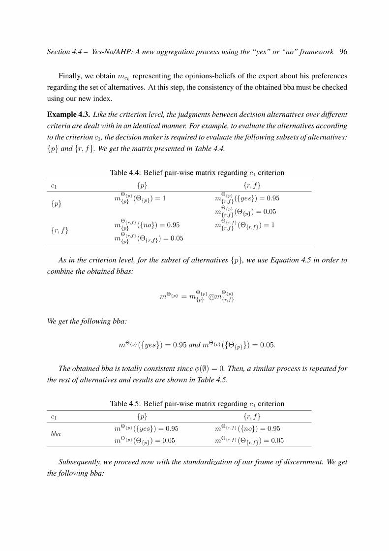
Section 4.4 – Yes-No/AHP: A new aggregation process using the “yes” or “no” framework 96
Finally, we obtain mck representing the opinions-beliefs of the expert about his preferencesregarding the set of alternatives. At this step, the consistency of the obtained bba must be checkedusing our new index.
Example 4.3. Like the criterion level, the judgments between decision alternatives over differentcriteria are dealt with in an identical manner. For example, to evaluate the alternatives accordingto the criterion c1, the decision maker is required to evaluate the following subsets of alternatives:p and r, f. We get the matrix presented in Table 4.4.
Table 4.4: Belief pair-wise matrix regarding c1 criterion
c1 p r, f
pm
Θpp (Θp) = 1 m
Θpr,f(yes) = 0.95
mΘpr,f(Θp) = 0.05
r, fm
Θr,fp (no) = 0.95 m
Θr,fr,f (Θr,f) = 1
mΘr,fp (Θr,f) = 0.05
As in the criterion level, for the subset of alternatives p, we use Equation 4.5 in order tocombine the obtained bbas:
mΘp = mΘpp ∩©m
Θpr,f
We get the following bba:
mΘp(yes) = 0.95 and mΘp(Θp) = 0.05.
The obtained bba is totally consistent since φ(∅) = 0. Then, a similar process is repeated forthe rest of alternatives and results are shown in Table 4.5.
Table 4.5: Belief pair-wise matrix regarding c1 criterion
c1 p r, f
bbamΘp(yes) = 0.95 mΘr,f(no) = 0.95
mΘp(Θp) = 0.05 mΘr,f(Θr,f) = 0.05
Subsequently, we proceed now with the standardization of our frame of discernment. We getthe following bba:
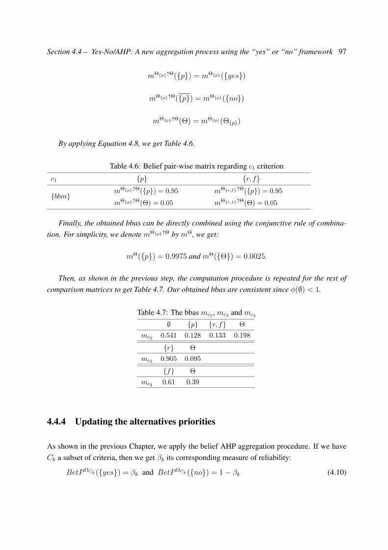
Section 4.4 – Yes-No/AHP: A new aggregation process using the “yes” or “no” framework 97
mΘp↑Θ(p) = mΘp(yes)
mΘp↑Θ(p) = mΘp(no)
mΘp↑Θ(Θ) = mΘp(Θp)
By applying Equation 4.8, we get Table 4.6.
Table 4.6: Belief pair-wise matrix regarding c1 criterion
c1 p r, f
bbmmΘp↑Θ(p) = 0.95 mΘr,f↑Θ(p) = 0.95
mΘp↑Θ(Θ) = 0.05 mΘr,f↑Θ(Θ) = 0.05
Finally, the obtained bbas can be directly combined using the conjunctive rule of combina-tion. For simplicity, we denote mΘp↑Θ by mΘ, we get:
mΘ(p) = 0.9975 and mΘ(Θ) = 0.0025.
Then, as shown in the previous step, the computation procedure is repeated for the rest ofcomparison matrices to get Table 4.7. Our obtained bbas are consistent since φ(∅) < 1.
Table 4.7: The bbas mc2 , mc3 and mc4
∅ p r, f Θ
mc2 0.541 0.128 0.133 0.198
r Θ
mc3 0.905 0.095
f Θ
mc4 0.61 0.39
4.4.4 Updating the alternatives priorities
As shown in the previous Chapter, we apply the belief AHP aggregation procedure. If we haveCk a subset of criteria, then we get βk its corresponding measure of reliability:
BetPΩCk (yes) = βk and BetPΩCk (no) = 1− βk (4.10)
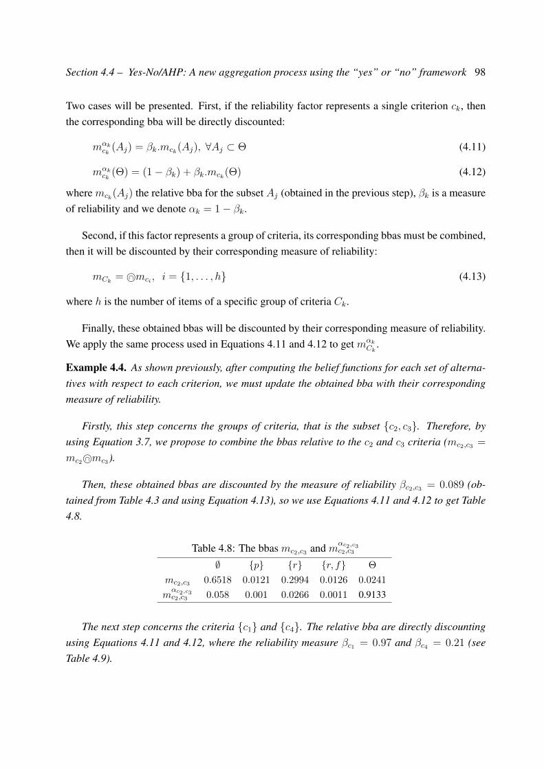
Section 4.4 – Yes-No/AHP: A new aggregation process using the “yes” or “no” framework 98
Two cases will be presented. First, if the reliability factor represents a single criterion ck, thenthe corresponding bba will be directly discounted:
mαkck
(Aj) = βk.mck(Aj), ∀Aj ⊂ Θ (4.11)
mαkck
(Θ) = (1− βk) + βk.mck(Θ) (4.12)
where mck(Aj) the relative bba for the subset Aj (obtained in the previous step), βk is a measureof reliability and we denote αk = 1− βk.
Second, if this factor represents a group of criteria, its corresponding bbas must be combined,then it will be discounted by their corresponding measure of reliability:
mCk= ∩©mci , i = 1, . . . , h (4.13)
where h is the number of items of a specific group of criteria Ck.
Finally, these obtained bbas will be discounted by their corresponding measure of reliability.We apply the same process used in Equations 4.11 and 4.12 to get mαk
Ck.
Example 4.4. As shown previously, after computing the belief functions for each set of alterna-tives with respect to each criterion, we must update the obtained bba with their correspondingmeasure of reliability.
Firstly, this step concerns the groups of criteria, that is the subset c2, c3. Therefore, byusing Equation 3.7, we propose to combine the bbas relative to the c2 and c3 criteria (mc2,c3 =
mc2 ∩©mc3).
Then, these obtained bbas are discounted by the measure of reliability βc2,c3 = 0.089 (ob-tained from Table 4.3 and using Equation 4.13), so we use Equations 4.11 and 4.12 to get Table4.8.
Table 4.8: The bbas mc2,c3 and mαc2,c3c2,c3
∅ p r r, f Θ
mc2,c3 0.6518 0.0121 0.2994 0.0126 0.0241
mαc2,c3c2,c3 0.058 0.001 0.0266 0.0011 0.9133
The next step concerns the criteria c1 and c4. The relative bba are directly discountingusing Equations 4.11 and 4.12, where the reliability measure βc1 = 0.97 and βc4 = 0.21 (seeTable 4.9).
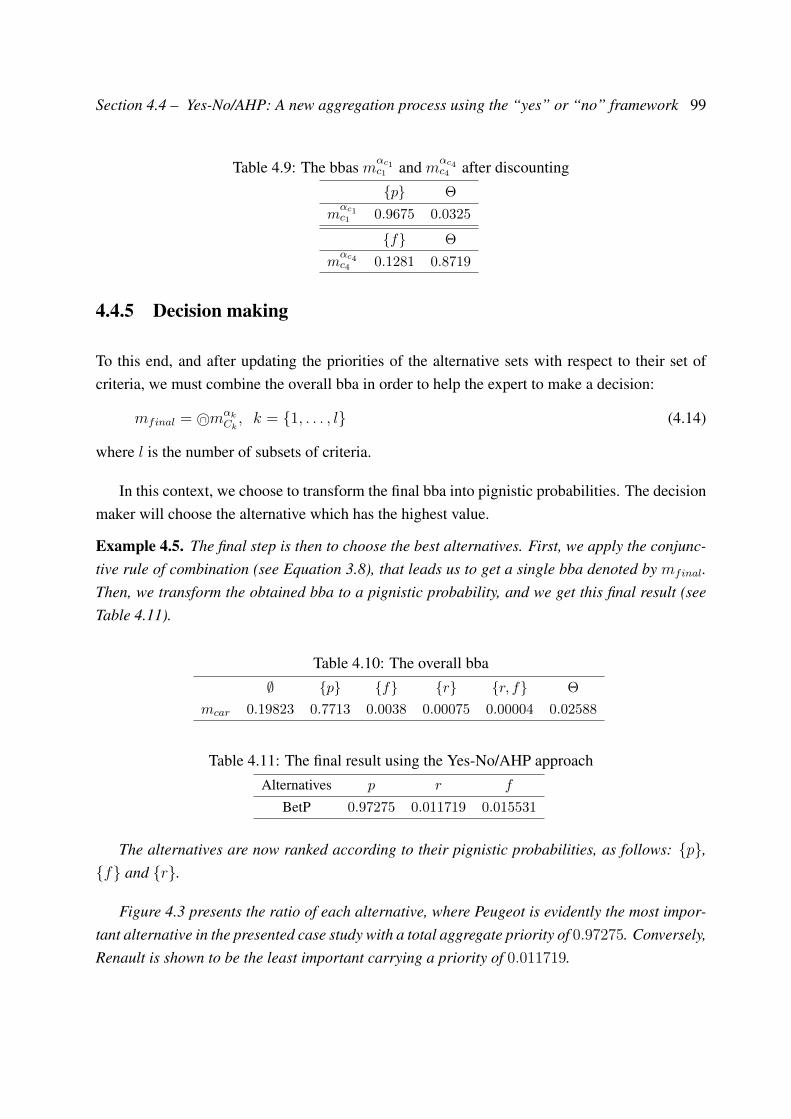
Section 4.4 – Yes-No/AHP: A new aggregation process using the “yes” or “no” framework 99
Table 4.9: The bbas mαc1c1 and mαc4
c4 after discountingp Θ
mαc1c1 0.9675 0.0325
f Θ
mαc4c4 0.1281 0.8719
4.4.5 Decision making
To this end, and after updating the priorities of the alternative sets with respect to their set ofcriteria, we must combine the overall bba in order to help the expert to make a decision:
mfinal = ∩©mαkCk, k = 1, . . . , l (4.14)
where l is the number of subsets of criteria.
In this context, we choose to transform the final bba into pignistic probabilities. The decisionmaker will choose the alternative which has the highest value.
Example 4.5. The final step is then to choose the best alternatives. First, we apply the conjunc-tive rule of combination (see Equation 3.8), that leads us to get a single bba denoted by mfinal.Then, we transform the obtained bba to a pignistic probability, and we get this final result (seeTable 4.11).
Table 4.10: The overall bba∅ p f r r, f Θ
mcar 0.19823 0.7713 0.0038 0.00075 0.00004 0.02588
Table 4.11: The final result using the Yes-No/AHP approachAlternatives p r f
BetP 0.97275 0.011719 0.015531
The alternatives are now ranked according to their pignistic probabilities, as follows: p,f and r.
Figure 4.3 presents the ratio of each alternative, where Peugeot is evidently the most impor-tant alternative in the presented case study with a total aggregate priority of 0.97275. Conversely,Renault is shown to be the least important carrying a priority of 0.011719.
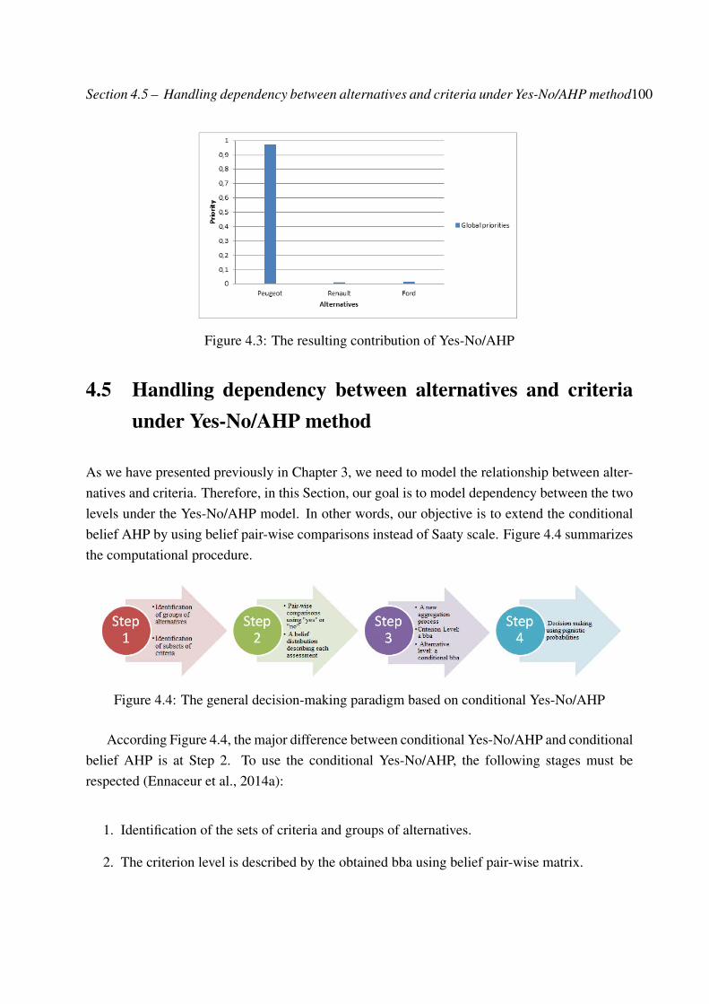
Section 4.5 – Handling dependency between alternatives and criteria under Yes-No/AHP method100
Figure 4.3: The resulting contribution of Yes-No/AHP
4.5 Handling dependency between alternatives and criteriaunder Yes-No/AHP method
As we have presented previously in Chapter 3, we need to model the relationship between alter-natives and criteria. Therefore, in this Section, our goal is to model dependency between the twolevels under the Yes-No/AHP model. In other words, our objective is to extend the conditionalbelief AHP by using belief pair-wise comparisons instead of Saaty scale. Figure 4.4 summarizesthe computational procedure.
Figure 4.4: The general decision-making paradigm based on conditional Yes-No/AHP
According Figure 4.4, the major difference between conditional Yes-No/AHP and conditionalbelief AHP is at Step 2. To use the conditional Yes-No/AHP, the following stages must berespected (Ennaceur et al., 2014a):
1. Identification of the sets of criteria and groups of alternatives.
2. The criterion level is described by the obtained bba using belief pair-wise matrix.
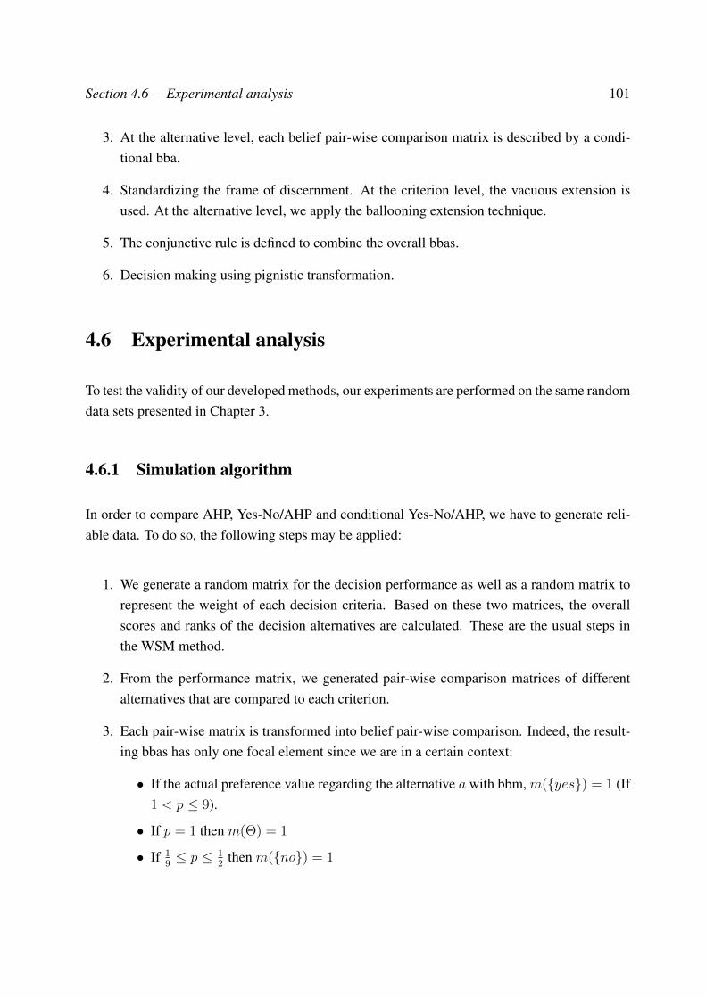
Section 4.6 – Experimental analysis 101
3. At the alternative level, each belief pair-wise comparison matrix is described by a condi-tional bba.
4. Standardizing the frame of discernment. At the criterion level, the vacuous extension isused. At the alternative level, we apply the ballooning extension technique.
5. The conjunctive rule is defined to combine the overall bbas.
6. Decision making using pignistic transformation.
4.6 Experimental analysis
To test the validity of our developed methods, our experiments are performed on the same randomdata sets presented in Chapter 3.
4.6.1 Simulation algorithm
In order to compare AHP, Yes-No/AHP and conditional Yes-No/AHP, we have to generate reli-able data. To do so, the following steps may be applied:
1. We generate a random matrix for the decision performance as well as a random matrix torepresent the weight of each decision criteria. Based on these two matrices, the overallscores and ranks of the decision alternatives are calculated. These are the usual steps inthe WSM method.
2. From the performance matrix, we generated pair-wise comparison matrices of differentalternatives that are compared to each criterion.
3. Each pair-wise matrix is transformed into belief pair-wise comparison. Indeed, the result-ing bbas has only one focal element since we are in a certain context:
• If the actual preference value regarding the alternative a with bbm, m(yes) = 1 (If1 < p ≤ 9).
• If p = 1 then m(Θ) = 1
• If 19≤ p ≤ 1
2then m(no) = 1
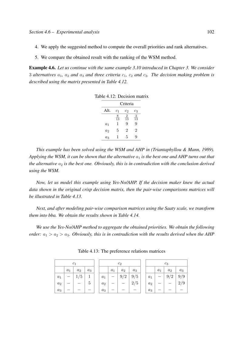
Section 4.6 – Experimental analysis 102
4. We apply the suggested method to compute the overall priorities and rank alternatives.
5. We compare the obtained result with the ranking of the WSM method.
Example 4.6. Let us continue with the same example 3.10 introduced in Chapter 3. We consider3 alternatives a1, a2 and a3 and three criteria c1, c2 and c3. The decision making problem isdescribed using the matrix presented in Table 4.12.
Table 4.12: Decision matrixCriteria
Alt. c1 c2 c3
813
213
313
a1 1 9 9
a2 5 2 2
a3 1 5 9
This example has been solved using the WSM and AHP in (Triantaphyllou & Mann, 1989).Applying the WSM, it can be shown that the alternative a1 is the best one and AHP turns out thatthe alternative a2 is the best one. Obviously, this is in contradiction with the conclusion derivedusing the WSM.
Now, let us model this example using Yes-No/AHP. If the decision maker knew the actualdata shown in the original crisp decision matrix, then the pair-wise comparisons matrices willbe illustrated in Table 4.13.
Next, and after modeling pair-wise comparison matrices using the Saaty scale, we transformthem into bba. We obtain the results shown in Table 4.14.
We use the Yes-No/AHP method to aggregate the obtained priorities. We obtain the followingorder: a1 > a2 > a3. Obviously, this is in contradiction with the results derived when the AHP
Table 4.13: The preference relations matrices
c1
a1 a2 a3
a1 − 1/5 1
a2 − − 5
a3 − − −
c2
a1 a2 a3
a1 − 9/2 9/5
a2 − − 2/5
a3 − − −
c3
a1 a2 a3
a1 − 9/2 9/9
a2 − − 2/9
a3 − − −
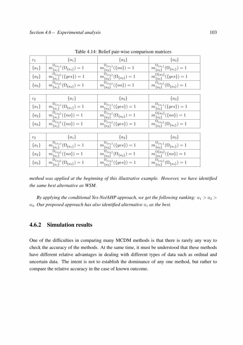
Section 4.6 – Experimental analysis 103
Table 4.14: Belief pair-wise comparison matrices
c1 a1 a2 a3
a1 mΩa1a1 (Ωa1) = 1 m
Ωa1a2 (no) = 1 m
Ωa1a3 (Ωa1) = 1
a2 mΩa2a1 (yes) = 1 m
Ωa2a2 (Ωa2) = 1 m
Ωa2a3 (yes) = 1
a3 mΩa3a1 (Ωa3) = 1 m
Ωa3a2 (no) = 1 m
Ωa3a3 (Ωa3) = 1
c2 a1 a2 a3
a1 mΩa1a1 (Ωa1) = 1 m
Ωa1a2 (yes) = 1 m
Ωa1a3 (yes) = 1
a2 mΩa2a1 (no) = 1 m
Ωa2a2 (Ωa2) = 1 m
Ωa2a3 (no) = 1
a3 mΩa3a1 (no) = 1 m
Ωa3a2 (yes) = 1 m
Ωa3a3 (Ωa3) = 1
c3 a1 a2 a3
a1 mΩa1a1 (Ωa1) = 1 m
Ωa1a2 (yes) = 1 m
Ωa1a3 (Ωa1) = 1
a2 mΩa2a1 (no) = 1 m
Ωa2a2 (Ωa2) = 1 m
Ωa2a3 (no) = 1
a3 mΩa3a1 (Ωa3) = 1 m
Ωa3a2 (yes) = 1 m
Ωa3a3 (Ωa3) = 1
method was applied at the beginning of this illustrative example. However, we have identifiedthe same best alternative as WSM.
By applying the conditional Yes-No/AHP approach, we get the following ranking: a1 > a2 >
a3. Our proposed approach has also identified alternative a1 as the best.
4.6.2 Simulation results
One of the difficulties in comparing many MCDM methods is that there is rarely any way tocheck the accuracy of the methods. At the same time, it must be understood that these methodshave different relative advantages in dealing with different types of data such as ordinal anduncertain data. The intent is not to establish the dominance of any one method, but rather tocompare the relative accuracy in the case of known outcome.
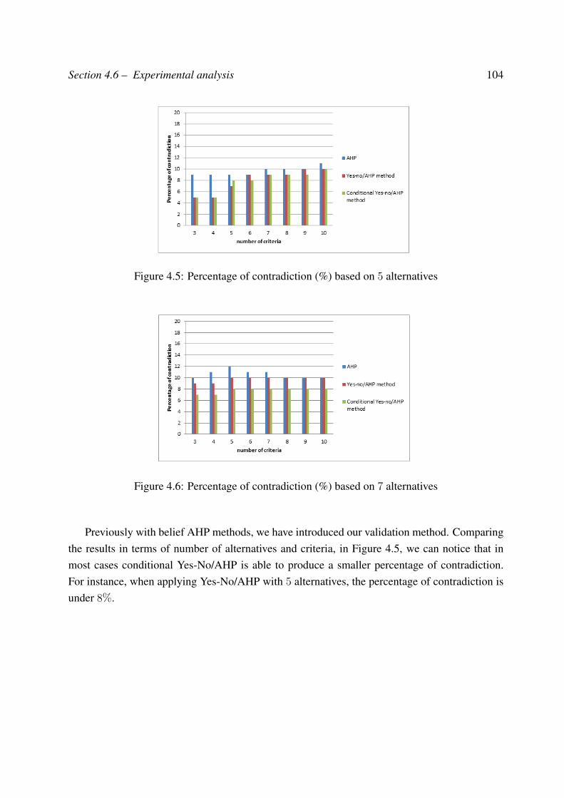
Section 4.6 – Experimental analysis 104
Figure 4.5: Percentage of contradiction (%) based on 5 alternatives
Figure 4.6: Percentage of contradiction (%) based on 7 alternatives
Previously with belief AHP methods, we have introduced our validation method. Comparingthe results in terms of number of alternatives and criteria, in Figure 4.5, we can notice that inmost cases conditional Yes-No/AHP is able to produce a smaller percentage of contradiction.For instance, when applying Yes-No/AHP with 5 alternatives, the percentage of contradiction isunder 8%.
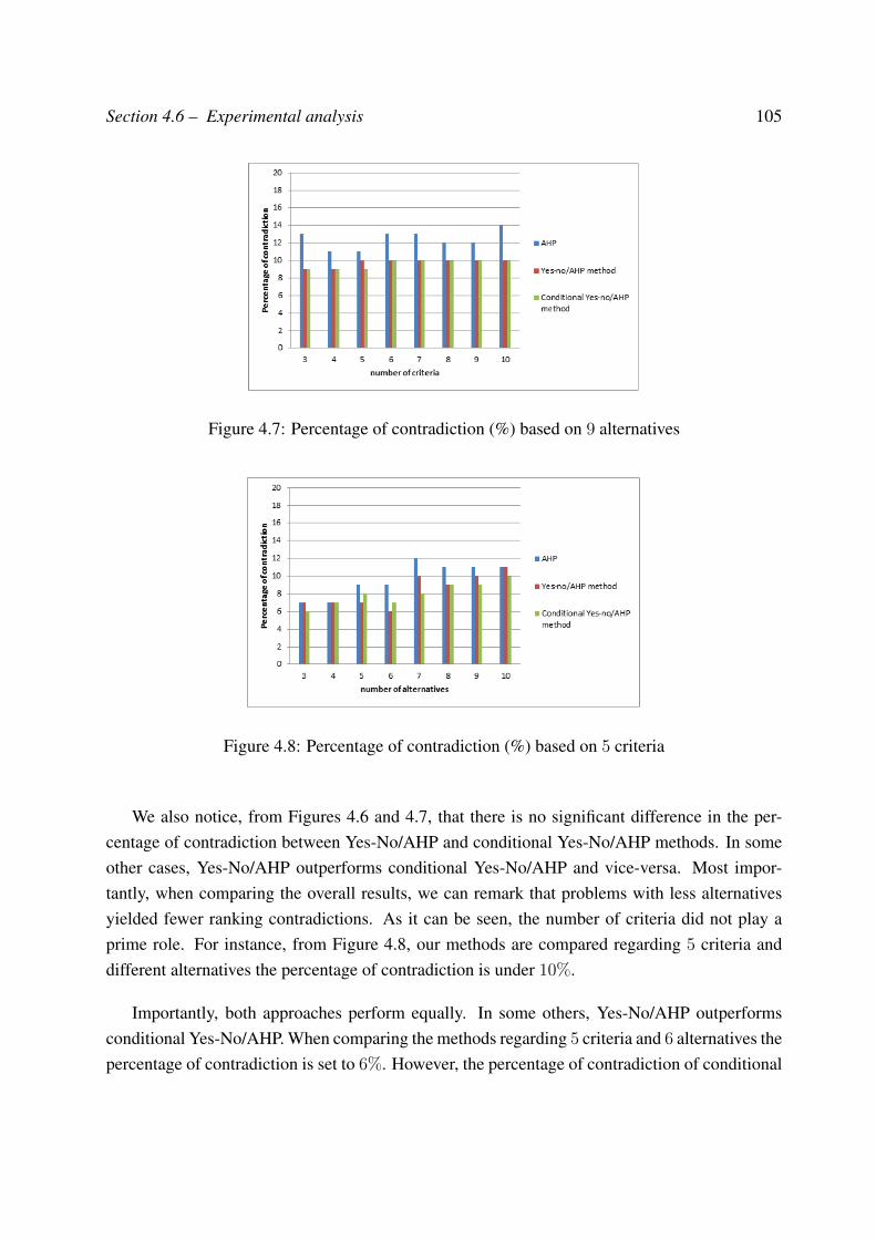
Section 4.6 – Experimental analysis 105
Figure 4.7: Percentage of contradiction (%) based on 9 alternatives
Figure 4.8: Percentage of contradiction (%) based on 5 criteria
We also notice, from Figures 4.6 and 4.7, that there is no significant difference in the per-centage of contradiction between Yes-No/AHP and conditional Yes-No/AHP methods. In someother cases, Yes-No/AHP outperforms conditional Yes-No/AHP and vice-versa. Most impor-tantly, when comparing the overall results, we can remark that problems with less alternativesyielded fewer ranking contradictions. As it can be seen, the number of criteria did not play aprime role. For instance, from Figure 4.8, our methods are compared regarding 5 criteria anddifferent alternatives the percentage of contradiction is under 10%.
Importantly, both approaches perform equally. In some others, Yes-No/AHP outperformsconditional Yes-No/AHP. When comparing the methods regarding 5 criteria and 6 alternatives thepercentage of contradiction is set to 6%. However, the percentage of contradiction of conditional
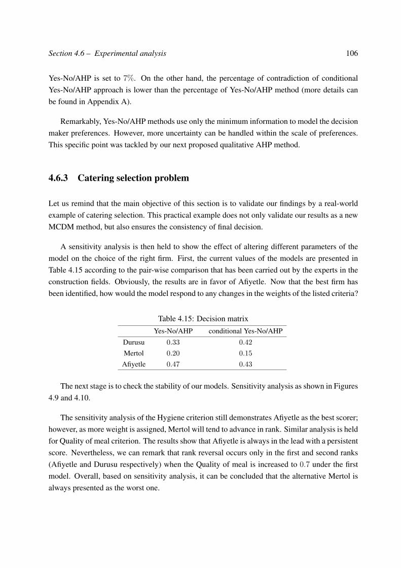
Section 4.6 – Experimental analysis 106
Yes-No/AHP is set to 7%. On the other hand, the percentage of contradiction of conditionalYes-No/AHP approach is lower than the percentage of Yes-No/AHP method (more details canbe found in Appendix A).
Remarkably, Yes-No/AHP methods use only the minimum information to model the decisionmaker preferences. However, more uncertainty can be handled within the scale of preferences.This specific point was tackled by our next proposed qualitative AHP method.
4.6.3 Catering selection problem
Let us remind that the main objective of this section is to validate our findings by a real-worldexample of catering selection. This practical example does not only validate our results as a newMCDM method, but also ensures the consistency of final decision.
A sensitivity analysis is then held to show the effect of altering different parameters of themodel on the choice of the right firm. First, the current values of the models are presented inTable 4.15 according to the pair-wise comparison that has been carried out by the experts in theconstruction fields. Obviously, the results are in favor of Afiyetle. Now that the best firm hasbeen identified, how would the model respond to any changes in the weights of the listed criteria?
Table 4.15: Decision matrixYes-No/AHP conditional Yes-No/AHP
Durusu 0.33 0.42
Mertol 0.20 0.15
Afiyetle 0.47 0.43
The next stage is to check the stability of our models. Sensitivity analysis as shown in Figures4.9 and 4.10.
The sensitivity analysis of the Hygiene criterion still demonstrates Afiyetle as the best scorer;however, as more weight is assigned, Mertol will tend to advance in rank. Similar analysis is heldfor Quality of meal criterion. The results show that Afiyetle is always in the lead with a persistentscore. Nevertheless, we can remark that rank reversal occurs only in the first and second ranks(Afiyetle and Durusu respectively) when the Quality of meal is increased to 0.7 under the firstmodel. Overall, based on sensitivity analysis, it can be concluded that the alternative Mertol isalways presented as the worst one.
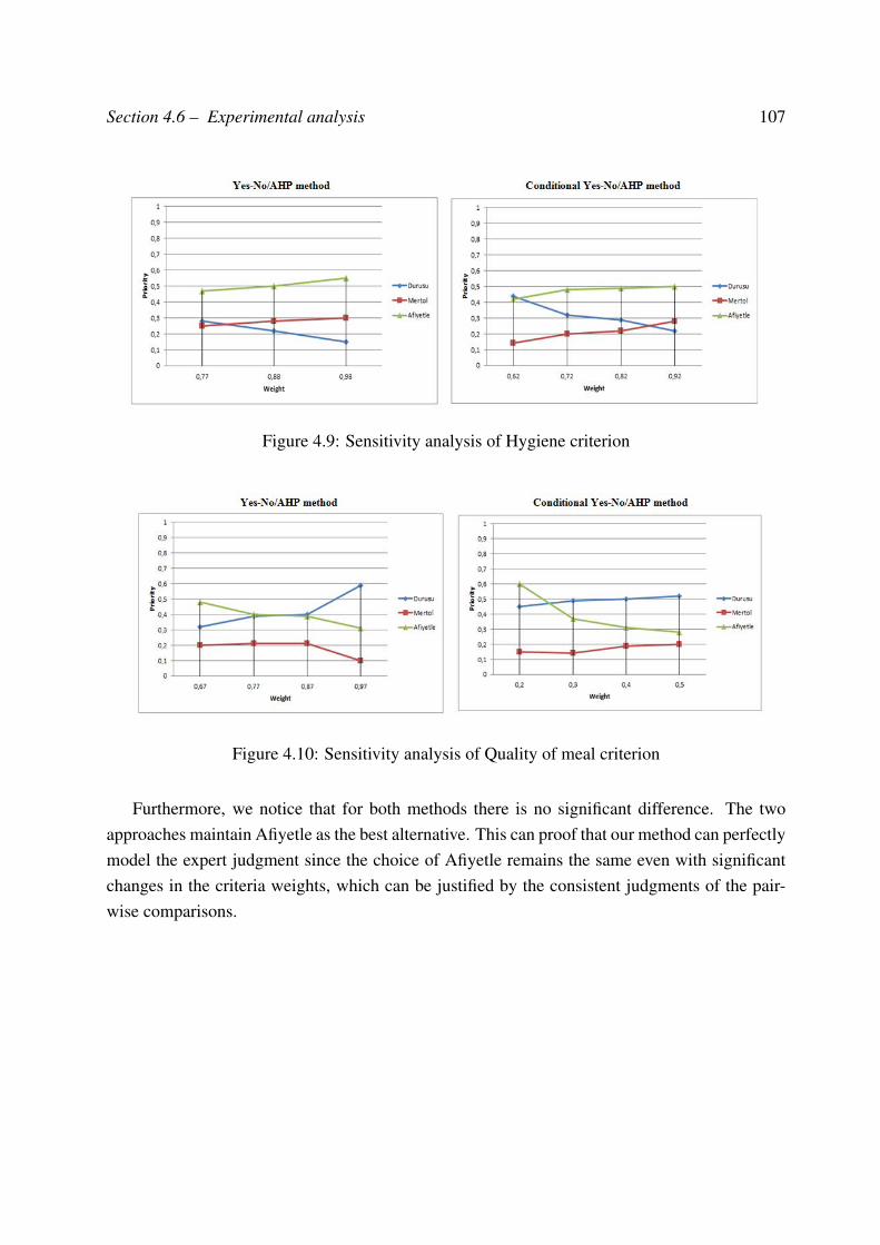
Section 4.6 – Experimental analysis 107
Figure 4.9: Sensitivity analysis of Hygiene criterion
Figure 4.10: Sensitivity analysis of Quality of meal criterion
Furthermore, we notice that for both methods there is no significant difference. The twoapproaches maintain Afiyetle as the best alternative. This can proof that our method can perfectlymodel the expert judgment since the choice of Afiyetle remains the same even with significantchanges in the criteria weights, which can be justified by the consistent judgments of the pair-wise comparisons.
Section 4.7 – Conclusion 108
4.7 Conclusion
In this Chapter, belief pair-wise comparison matrix was developed. We have exposed what kindof uncertainty is handled by this technique as well as its different objectives. Then, new AHPextensions were defined based on belief pair-wise procedure. We have explained their main stepsand evaluated their performance using generated random data.
Despite the noticed advantages of our proposed Yes-No/AHP methods, there are some lim-itations. In some cases, the decision maker cannot estimate his assessment with a numericalvalue. This prompted our research into the use of qualitative belief function method in order togenerate quantitative information from qualitative assessments. This will be dealt with in thenext Chapter.
Chapter 5Constructing belief functions fromqualitative expert assessments
5.1 Introduction
For many years, qualitative methods for reasoning under uncertainty have increasingly attractedpeople (Parsons, 1994; Wong & Lingras, 1994). Their aim is to propose solutions for process-ing qualitative information which efficiently take into account information provided by humansources. The aim of qualitative reasoning methods is to help in decision-making for situationsin which the precise numerical methods are not appropriate (Parsons & Hunter, 1998). Severalformalisms for qualitative reasoning have been proposed by Ben Yaghlane et al. (2006), Brysonand Mobolurin (1999), Parsons (1994), and Wong and Lingras (1994).
However, modeling the decision maker’s preferences is not an easy task because he usuallyprefers to express his opinions in natural language based on knowledge and experience that heprovides rather than direct quantitative information. In other words, solving a problem dealingwith the expert’s preferences is usually characterized by a high degree of uncertainty. Besides,in some cases, the decision maker may be unable to express his opinions due to his lack ofknowledge. He is then forced to provide incomplete or even erroneous information. Obviously,ignoring this difficulty in eliciting the expert’s preference is not a good practice. Therefore,preferences need to be implemented in an assessment, which reflects as accurately as possiblethe human mind.
109
Section 5.2 – Motivations 110
To tackle the problem, a numerical representation under the belief function framework isintroduced.
In order to do this, this Chapter is set out as follows. First, in Section 5.2, we give somemotivations. We recall in Section 5.3 what can be called preference modeling which servesas a “benchmark” for most of the works in the area. Then, we provide a brief description ofsome existing qualitative reasoning methods (Section 5.4). Next, in Section 5.5, our suggestedsolutions are described and examples are presented to illustrate our methods.
5.2 Motivations
When solving problems dealing with belief function theory, experts are usually required to pro-vide precise numerical value, for determining the portion of belief committed exactly to an eventin a particular domain. However, when handling such a situation, the main difficulty is how toquantify these numeric values. Therefore, linguistic assessments could be used instead. The ex-pert is then asked to express his opinions qualitatively based on knowledge and experience thathe provides in response to a given question rather than direct quantitative information.
Besides, in preference modeling, the expert may express preferences towards a pair of alter-natives in distinct ways: he either has a strict preference towards one alternative, or is indifferentto both alternatives. These two interpretations are possible because we made the assumptionbased on complete and certain information.
However, these two preferences do not apply to all possible situations that a decision makermay faced. Consider now the situations in which the expert has symmetrically lack and excess ofinformation in the sense that he has contradictory inputs. He is then forced to provide incompleteor even erroneous information.
Consequently, new situations are introduced, such as incompleteness and incomparability.The intuition is that the expert cannot compare apple and cheese because they are too different.For instance, he may consider that alternatives may be incomparable because the expert doesnot wish very dissimilar alternatives to be compared. Incompleteness, on the other hand, simplyrepresents an absence of knowledge about the preference of certain pairs of alternatives. It ariseswhen we have not fully elicited an expert’s preferences or when the expert does not have thefull information. Moreover, we suggest to include the weak preference relation (Roy, 1987), that
Section 5.3 – Binary Relations and Preference Modeling 111
separates the preference area from the indifference area. A possible interpretation is an hesitationbetween strict preference and indifference.
To deal with such situations, a more realistic solution is proposed, that is able to efficientlyimitate the expert’s reasoning using belief function theory (Ennaceur et al., 2012a, 2013a, 2014b).Our main aim is then to elaborate on how may be incomparability, incompleteness and weakpreference be represented in the belief function framework. In the next Section, we will start byintroducing some classical binary relations.
5.3 Binary Relations and Preference Modeling
The literature on preference modeling is vast. This can first be explained by the fact that thequestion of modeling preferences occurs in several disciplines, such as the following:
• in Economics, where we try to model the preferences of a rational consumer (Debreu,1959).
• in Psychology, in which the study of preference judgments collected in experiments isquite common (Kahneman & Tversky, 1979).
• in Political Sciences, in which the question of defining a collective preference on the basisof the opinion of several voters is central (Sen, 1986).
• in Operations Research, in which optimizing an objective function implies the definitionof a direction of preference (Roy, 1985).
• in Artificial Intelligence, in which the creation of autonomous agents able to make deci-sions involves the modeling of their vision of what is desirable and what is less so (Doyle& Wellman, 1992).
A binary relation T on a setA is a subset of the Cartesian productA×A, i.e. a set of ordered pairs(a, b) of elements of A. If the ordered pair (a, b) belongs to the set T , we will often write aTb. Inthe opposite case, we write aT b. Except when explicitly mentioned otherwise, we will supposein all what follows that the set A is finite (Roubens & Vincke, 1985; Bouyssou & Vincke, 2009).
Consider an ordered pair (a, b) of objects. In the classical theory, it is supposed that theanswer to the question: is a least as good as b? can only have two possible answers: yes or no.
Section 5.3 – Binary Relations and Preference Modeling 112
Asking such a question for all possible ordered pairs of objects defines a binary relation on T inthe following way:
aTb iff the answer to the question “is a at least as good as b?” “is yes”.
It is easy to see that considering a pair (a, b) of objects, four and only four mutually exclusivecases arise:
• aTb ∧ bTa denoted by a ∼ b, which reads “a is indifferent to b”,
• Not aTb ∧ Not bTa denoted by a?b, which reads “a is incomparable to b”,
• aTb ∧ Not bTa denoted by a b, which reads “a is strictly preferred to b”,
• Not aTb ∧ bTa denoted by b a, which reads “b is strictly preferred to a”.
In some cases, we may consider answers other than yes or no to the question “is a at least asgood as b?”, such as the following:
• answers such as I do not know,
• answers including information on the intensity of the preference,
• answers including information on the credibility of the proposition.
Admitting such answers imply using a language that is richer than that of binary relations,e.g.:
• the language of fuzzy relations, each assertion of the type aSb having a degree of credibility(Doignon et al., 1986),
• languages tolerating hesitation (Perny & Roy, 1992),
• languages using the idea of intensity of preference (Doignon, 1987; Costa & Vansnick,1994), an assertion such that aSb and bSa being further qualified (weak, strong or extremepreference, for instance).
Therefore, in this Chapter, we introduce a new elicitation method under the belief function frame-work, based on preference relations. We start by describing some existing approaches. Then, wewill present our proposed solution.

Section 5.4 – Overview of qualitative reasoning methods 113
5.4 Overview of qualitative reasoning methods
The problem of qualitatively eliciting experts’ opinions and generating basic belief assignmentshave been addressed by many researchers: Wong and Lingras (1994), Parsons (1994), Brysonand Mobolurin (1999) and Ben Yaghlane et al. (2006). In this Section, we provide an overviewof some existing approaches.
5.4.1 Wong and Lingras’ Method
Wong and Lingras (1994) proposed a method for generating quantitative belief functions fromqualitative preference assessments. So, given a pair of propositions, experts may express whichof the propositions is more likely to be true. Thus, they defined two binary relations: preference() and indifference (∼) defined on 2Θ such as:
a b is equivalent to bel(a) > bel(b) (5.1)
a ∼ b is equivalent to bel(a) = bel(b) (5.2)
where a, b ∈ 2Θ.
This approach is based on two steps. The first one consists in considering that all the proposi-tions that appear in the preference relations are potential focal elements. However, some propo-sitions are eliminated according to the following condition: if a ∼ b for some a ⊂ b, then a isnot a focal element.
After that, the basic belief assignment is generated using the two presented Equations 5.1 and5.2. This formulation has multiple belief functions that are consistent with the input qualitativeinformation, and so their procedure only generates one of them.
It should be noted that Wong and Lingras’ approach does not address the issue of incon-sistency in the pair-wise comparisons. For example, the expert could specify the apparentlyinconsistent preference relationships: bel(a) > bel(b), bel(b) > bel(c) and bel(c) > bel(a).
Section 5.4 – Overview of qualitative reasoning methods 114
5.4.2 Parsons Method
Parsons (1994) suggests a qualitative approach in which the mass of each proposition is expressedvaguely. He defines a qualitative mass function [m(A)] that corresponds to m(A).
if m(A) > 0, then [m(A)] = + (5.3)
if m(A) = 0, then [m(A)] = 0
where + is any mass that is known to be non-zero (0 < + < 1).
He demonstrates how these qualitative mass functions can be combined based on the Demp-ster combination rule. Parsons (1994) further suggests that linguistic quantifiers can be usedto aid the transformation from qualitative representation of belief to numeric representation ofbelief. He suggested the linguistic qualifiers None, Little, About Half, Much, All where:
None ≤ Little ≤ About Half ≤Much ≤ All.
with each linguistic qualifier corresponding to a subinterval of the unit interval [0, 1].
Parsons also suggests that bba could be represented numerically using numeric intervals. Henotes that this approach gives more precise results than the linguistic approach because inter-vals do not have to be rounded to the nearest numeric interval. With this approach it becomesnecessary to do interval ranking, which could be done using fuzzy arithmetic.
5.4.3 Bryson Method
Qualitative Discrimination Process (QDP), a model for generating belief functions from qualita-tive preferences, was presented by Bryson and Mobolurin (1999).
This method is based on the following steps. First, using this QDP approach, each propositionis assigned into a broad category bucket, then to a corresponding intermediate bucket and finallyto a corresponding narrow category bucket. The qualitative scoring is done using a table whereeach broad category is a linguistic quantifier in the sense of Parsons (1994). He considers thatlinguistic quantifiers could provide a useful approach to representing beliefs vaguely. Hence bbashould be represented using numeric intervals.
Section 5.4 – Overview of qualitative reasoning methods 115
Then, in Step 2, the previous broad category is used to identify and remove non focal propo-sitions. For each superset proposition, determine if the expert is indifferent in his strength ofbelief, in the truthfulness of the given proposition and any of its subset propositions in the sameor lower narrow category bucket.
Step 3 is called “imprecise pair-wise comparisons” because the expert is required to providenumeric intervals to express his beliefs on the relative truthfulness of the propositions.
In Step 4, the consistency of the belief information provided by the expert is checked. Then,the belief function is generated in Step 5 by providing a bba interval for each focal element.
Finally, in Step 6, the expert examines the generated belief functions and stops the QDP if itis acceptable, otherwise the process is repeated.
5.4.4 Ben Yaghlane et al.’s Method
Ben Yaghlane et al. (2006) proposed a method for generating optimized belief functions fromqualitative preferences.
So given two alternatives, an expert can usually express which of the propositions is morelikely to be true, thus he used two binary preference relations: the preference and the indifferencerelations.
The objective of this method is then to convert these preferences into constraints of an op-timization problem whose resolution, according to some uncertainty measures (UM) (nonspeci-ficity measures, conflict measures, composite measures (see Section 2.3.4)), allows the genera-tion of the least informative or the most uncertain belief functions defined as follows:
a b⇔ bel(a)− bel(b) ≥ ε (5.4)
a ∼ b⇔ |bel(a)− bel(b)| ≤ ε (5.5)
where ε is considered to be the smallest gap that the expert may discern between the degreesof belief in two propositions a and b. Note that ε is a constant specified by the expert beforebeginning the optimization process.
Ben Yaghlane et al. (2006) propose a method which requires that propositions are representedin terms of focal elements, they assume that Θ (where Θ is the frame of discernment) should
Section 5.4 – Overview of qualitative reasoning methods 116
always be considered as a potential focal element. Then, a mono-objective technique was usedto solve such constrained optimization problem:
MaxmUM(m)
s.t.
bel(a)− bel(b) ≥ ε ∀(a, b) for which a b
bel(a)− bel(b) ≥ −ε ∀(a, b) for which a ∼ b
bel(a)− bel(b) ≤ ε ∀(a, b) for which a ∼ b∑a∈F(m)
m(a) = 1,m(a) ≥ 0,∀a ⊆ Θ;m(∅) = 0
(5.6)
where the first, second and third constraints are derived from Equations 5.4 and 5.5, representingthe quantitative constraints that correspond to the qualitative preference relations.
Furthermore, the proposed method addresses the problem of inconsistency. In fact, if thepreference relations are consistent, then the optimization problem is feasible. Otherwise nosolutions will be found. Thus, the expert may be guided to reformulate his preferences.
An extension of the proposed solution is also presented. In fact, they suggested to use thegoal programming, a multiobjective method, in order to take into account several objectivessimultaneously in the formulation of the problem. So, the idea behind the use of this method isto be able to integrate additional information about the belief functions to be generated.
It should be noted that this method does not address the issue of incomparability in the pair-wise comparisons. In fact, this proposed method treats incomparability as incompleteness. How-ever, we believe that this interpretation is not appropriate. If an expert is unable to compare twoalternatives then this situation should be reflected in the preference relation not as an incom-plete situation, but with an entry for that particular pair of alternatives. Moreover, we suggestto include the weak preference relation, that separates the preference area from the indifferenceone. A possible interpretation is hesitation between strict preference and indifference. So, in thefollowing Section, we present our method which deals with these problems.

Section 5.5 – A new elicitation method using qualitative assessments 117
5.5 A new elicitation method using qualitative assessments
As presented above, efficiently representing the expert’s preferences is a crucial task in elaborat-ing the necessary data for a considered problem. Therefore, we propose a realistic solution thatis able to efficiently imitate the expert’s reasoning.
Our first step is then to elaborate on how may incomparability and incompleteness be rep-resented in qualitative belief functions. The solution we suggest is then a qualitative model forconstructing belief functions from elicited experts’ opinions when dealing with qualitative pref-erence relations based only on strict preference and indifference relations. The second stage is tointroduce the weak preference relation, that separates the preference area from the indifferenceone by inserting an intermediate zone.
5.5.1 Preference articulation: Incompleteness
Incomparability and incompleteness represent very different concepts. In this subsection, we tryto differentiate incomplete preferences from incomparable ones. This situation is illustrated bycomplete ignorance, missing information, lack of knowledge or an ongoing preference elicitationprocess. Incompleteness represents then simply an absence of knowledge of the relationshipbetween these pairs of alternatives.
Given such considerations, it may perhaps be useful at times to take incomplete order as theprimitive of analysis. Besides, the expert is freely allowed to assign this belief to any pairs ofalternatives. In other words, a partial order allows some relations between pairs of alternatives tobe unknown.
Example 5.1. Given three alternatives Θ = a, b, c, an incomplete order can be for example:(a c, b ∼ c) or (c a, a ∼ b), where some relations between pairs of alternatives areunknown.
5.5.2 Preference articulation: Incomparability
A missing value in a linguistic preference relation is not always equivalent to a lack of preferenceof one alternative rather than another. A missing value can also be the result of an expert’s
Section 5.5 – A new elicitation method using qualitative assessments 118
inability to compare one alternative to another because they are too different. In such cases, theexpert may not put his opinion about certain aspects of the problem; he would not be able toefficiently express his preference towards two or more of the available alternative. As a result,he may find some of them to be incomparable and thus has an incomplete preference ordering,i.e., he neither prefers one alternative over the other nor finds them equally as good. Therefore, itwould be of great importance to provide the expert with tools that would him allow to efficientlymodel his preferences.
In order to model this situation, we first consider how to represent the incomparability relation(?). Our problem here is that incomparability is expressed entirely in terms of negations:
a?b iff ¬(a b) ∧ ¬(b a) (5.7)
By definition, a couple of alternatives (a, b) belongs to the incomparability relation if andonly if the expert is unable to compare a and b. Furthermore, it is hard to see what kind ofbehavior could correspond to Equation 5.7. If neither a nor b is chosen, the expert may not beable to tell which alternative is better, since not a b, not b a and not a ∼ b. In other terms, weapply incomparability when the preference profiles of two alternatives are severely conflicting.
The question now is how to formalize this situation in the belief function framework. Inorder to build this new preference relation, we may accept that there exist positive reasons whichsupport the relation ¬(a b) and also there exists sufficient negative information to establishthe relation (a b). These two assumptions can properly model the contradictory information.Besides, we can surely establish that “a is preferred to b” as there are not sufficient reasonssupporting the opposite, and there are sufficient information against it, while we can also surelyestablish that “b is preferred to a” for the same reasons. Therefore, a and b are in a conflictingposition.
On the other hand, and based on the belief function framework and as defined by Boujelben etal. (2011), the incomparability situation appears between two alternatives when their evaluationsgiven by basic belief assessments differ significantly.
Consider two alternatives a and b, as proved in Wong and Lingras (1994); the belief functionexists since the preference relation satisfies the following axioms:
1. Asymmetry: a b⇒ ¬(b a)
2. Negative Transitivity: ¬(a b) ∧ ¬(b c)⇒ ¬(a c)
Section 5.5 – A new elicitation method using qualitative assessments 119
3. Dominance: ∀ a, b ∈ 2Θ, a ⊇ b⇒ a b or a ∼ b
4. Partial monotonicity: ∀ a, b, c ∈ 2Θ, if a ⊃ b and a ∩ c = ∅ ⇒ (a ∪ c) (b ∪ c)
According to Wong and Wong and Lingras (1994), functions other than the belief ones mayexist, which are also compatible with a preference relation such that for every a, b ∈ 2Θ:
a b⇔ f(a) ≥ f(b) (5.8)
if and only if the relation satisfies the previous axioms.
Similarly to this idea, we can prove that the plausibility function also exists since the pref-erence relation satisfies the previous axioms. Besides, we can conclude that there exists aplausibility function pl: 2Θ → [0, 1] such as:
a b⇔ pl(a) ≥ pl(b) (5.9)
To summarize, we can get the following relations:
a b⇔ bel(a) ≥ bel(b) and pl(a) ≥ pl(b) (5.10)
As we have defined previously, the incomparability situation appears between two alterna-tives when their preference profiles are severely conflicting. That is when their evaluations givenby basic belief assessments differ significantly. We can then intuitively conclude from Equation5.10 that, if a is incomparable with b, then:
pl(a) ≤ pl(b) ∧ bel(a) ≥ bel(b) (5.11)
The first part of Equation 5.11 supports the assumption “a is preferred to b”; however, thesecond one supports the opposite claim. Also, the second part of the equation supports theassumption “b is preferred to a” and the first part affirms the opposite assumption.
Consequently, our purpose is then to prove the existence of the previous Equation 5.11 inorder to correctly represent the bba relative to the incomparability relation.
Demonstration
a?b⇔ ¬(pl(a) ≥ pl(b)) ∧ ¬(bel(b) ≥ bel(a)) (5.12)
Section 5.5 – A new elicitation method using qualitative assessments 120
Then:
pl(b) ≥ pl(a) ∧ bel(a) ≥ bel(b) (5.13)
⇔ pl(a) ≤ pl(b) ∧ bel(a) ≥ bel(b) (5.14)
As a result, we obtain the relation presented in Equation 5.11.
We propose the following proof to justify the previous relation:
pl(a) ≤ pl(b)⇔ bel(Θ)− bel(a) ≤ bel(Θ)− bel(b)
⇔ −bel(a) ≤ −bel(b)
⇔ bel(a) ≥ bel(b)
However, we replace in Equation 5.14 pl(a) ≤ pl(b) by bel(a) ≥ bel(b). We obtain:
bel(a) ≥ bel(b) ∧ bel(a) ≥ bel(b) (5.15)
Then:
[bel(a) > bel(b) ∨ bel(a) = bel(b)] ∧ [bel(a) > bel(b) ∨ bel(a) = bel(b)] (5.16)
Moreover:
[a b ∨ a ∼ b] ∧ [a b ∨ a ∼ b] (5.17)
Also, we have:
a ∼ b⇔ a b ∧ b a (5.18)
As a result:
[a b ∨ (a b ∧ b a)] ∧ [a b ∨ (a b ∧ b a)] (5.19)
Then, we apply the absorption law: A ∨ A ∧B = A
⇒ [a b] ∧ [a b] (5.20)
Section 5.5 – A new elicitation method using qualitative assessments 121
Besides, we have:
¬(a b) ∧ a b (5.21)
As a result:
¬(a b) ∧ ¬(b a) (5.22)
Finally, we obtain the incomparability relation.
As a conclusion, such representation of incomparability (see Equation 5.10) enables us tocorrectly express the conflicting information produced by the alternative a and the alternative b.In fact, the first part of the Equation 5.11 “bel(a) ≥ bel(b)” implies that a is preferred to b. Then,the plausibility function is used since it expresses the maximum amount of specific support thatcould be given to a proposition a. However, when we define the second part of the Equation 5.11,we propose to assume that pl(a) ≤ pl(b) which means that b is preferred to a. This contradictswith the first assumption and can properly express the conflicting information produced by a andb. Using this relation some new focal elements may appear two express the conflicting relation.
Computational procedure
Now and after modeling the incompleteness and the incomparability preferences, we propose toextend Ben Yaghlane et al. method (Ben Yaghlane et al., 2006). We transform these preferencerelations into constraints. We get:
MaxmUM(m)
s.t.
bel(a)− bel(b) ≥ ε ∀(a, b) for which a b
bel(a)− bel(b) ≤ ε ∀(a, b) for which a ∼ b
bel(a)− bel(b) ≥ −ε ∀(a, b) for which a ∼ b
bel(a) ≥ bel(b) ∀(a, b) for which a?b
pl(a) ≤ pl(b) ∀(a, b) for which a?b∑a∈F(m)
m(a) = 1;m(a) ≥ 0;∀a ⊆ Θ;m(∅) = 0
(5.23)
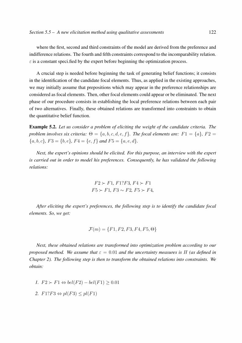
Section 5.5 – A new elicitation method using qualitative assessments 122
where the first, second and third constraints of the model are derived from the preference andindifference relations. The fourth and fifth constraints correspond to the incomparability relation.ε is a constant speci.fied by the expert before beginning the optimization process.
A crucial step is needed before beginning the task of generating belief functions; it consistsin the identification of the candidate focal elements. Thus, as applied in the existing approaches,we may initially assume that prepositions which may appear in the preference relationships areconsidered as focal elements. Then, other focal elements could appear or be eliminated. The nextphase of our procedure consists in establishing the local preference relations between each pairof two alternatives. Finally, these obtained relations are transformed into constraints to obtainthe quantitative belief function.
Example 5.2. Let us consider a problem of eliciting the weight of the candidate criteria. Theproblem involves six criteria: Θ = a, b, c, d, e, f. The focal elements are: F1 = a, F2 =
a, b, c, F3 = b, e, F4 = e, f and F5 = a, e, d.
Next, the expert’s opinions should be elicited. For this purpose, an interview with the expertis carried out in order to model his preferences. Consequently, he has validated the followingrelations:
F2 F1, F1?F3, F4 F1
F5 F1, F3 ∼ F2, F5 F4,
After eliciting the expert’s preferences, the following step is to identify the candidate focalelements. So, we get:
F(m) = F1, F2, F3, F4, F5,Θ
Next, these obtained relations are transformed into optimization problem according to ourproposed method. We assume that ε = 0.01 and the uncertainty measures is H (as defined inChapter 2). The following step is then to transform the obtained relations into constraints. Weobtain:
1. F2 F1⇔ bel(F2)− bel(F1) ≥ 0.01
2. F1?F3⇔ pl(F3) ≤ pl(F1)
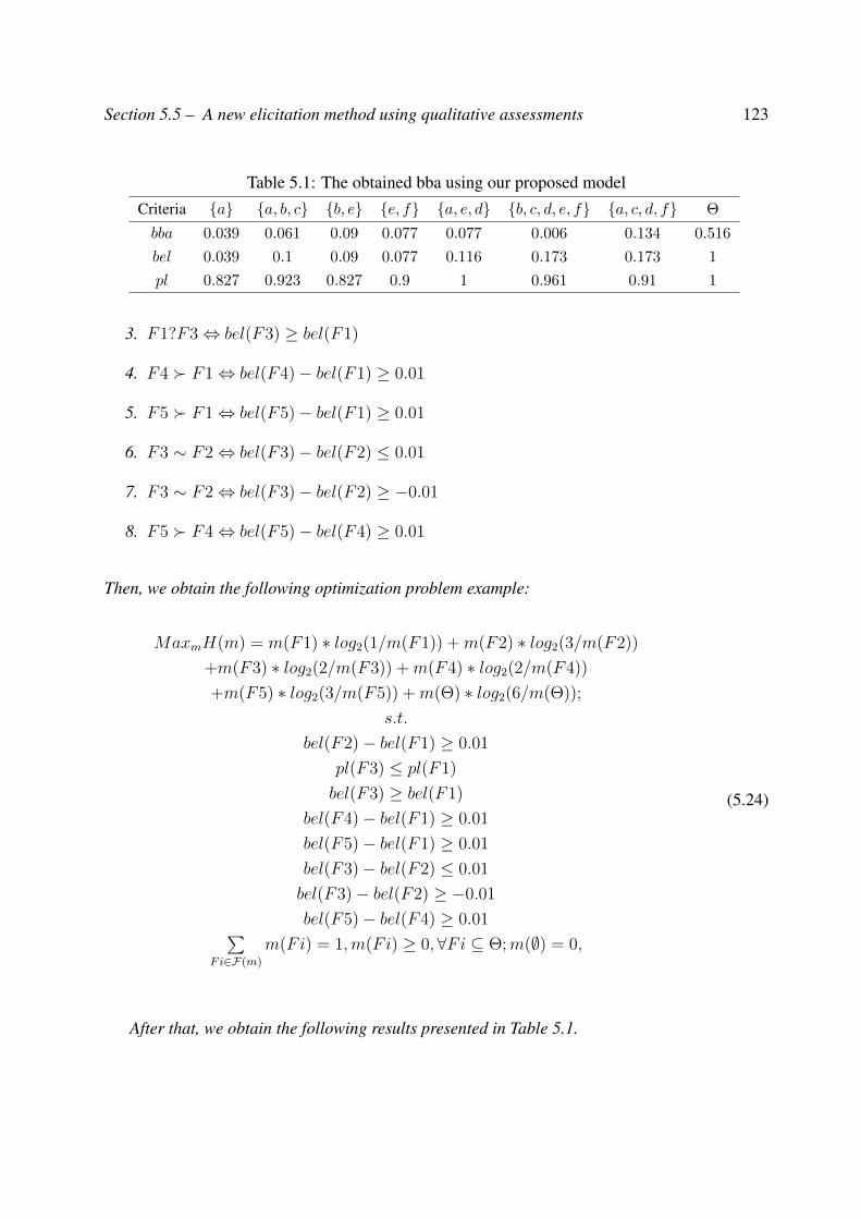
Section 5.5 – A new elicitation method using qualitative assessments 123
Table 5.1: The obtained bba using our proposed modelCriteria a a, b, c b, e e, f a, e, d b, c, d, e, f a, c, d, f Θ
bba 0.039 0.061 0.09 0.077 0.077 0.006 0.134 0.516
bel 0.039 0.1 0.09 0.077 0.116 0.173 0.173 1
pl 0.827 0.923 0.827 0.9 1 0.961 0.91 1
3. F1?F3⇔ bel(F3) ≥ bel(F1)
4. F4 F1⇔ bel(F4)− bel(F1) ≥ 0.01
5. F5 F1⇔ bel(F5)− bel(F1) ≥ 0.01
6. F3 ∼ F2⇔ bel(F3)− bel(F2) ≤ 0.01
7. F3 ∼ F2⇔ bel(F3)− bel(F2) ≥ −0.01
8. F5 F4⇔ bel(F5)− bel(F4) ≥ 0.01
Then, we obtain the following optimization problem example:
MaxmH(m) = m(F1) ∗ log2(1/m(F1)) +m(F2) ∗ log2(3/m(F2))
+m(F3) ∗ log2(2/m(F3)) +m(F4) ∗ log2(2/m(F4))
+m(F5) ∗ log2(3/m(F5)) +m(Θ) ∗ log2(6/m(Θ));
s.t.
bel(F2)− bel(F1) ≥ 0.01
pl(F3) ≤ pl(F1)
bel(F3) ≥ bel(F1)
bel(F4)− bel(F1) ≥ 0.01
bel(F5)− bel(F1) ≥ 0.01
bel(F3)− bel(F2) ≤ 0.01
bel(F3)− bel(F2) ≥ −0.01
bel(F5)− bel(F4) ≥ 0.01∑Fi∈F(m)
m(Fi) = 1,m(Fi) ≥ 0,∀Fi ⊆ Θ;m(∅) = 0,
(5.24)
After that, we obtain the following results presented in Table 5.1.
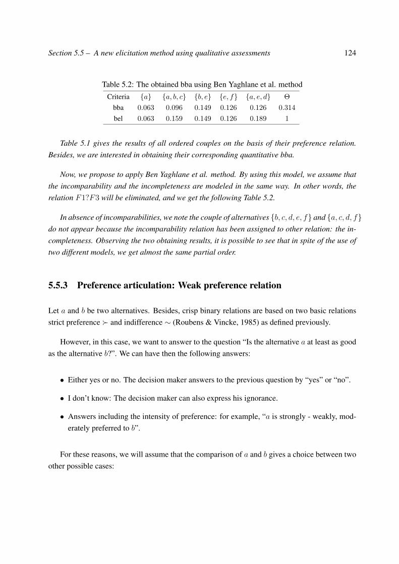
Section 5.5 – A new elicitation method using qualitative assessments 124
Table 5.2: The obtained bba using Ben Yaghlane et al. methodCriteria a a, b, c b, e e, f a, e, d Θ
bba 0.063 0.096 0.149 0.126 0.126 0.314
bel 0.063 0.159 0.149 0.126 0.189 1
Table 5.1 gives the results of all ordered couples on the basis of their preference relation.Besides, we are interested in obtaining their corresponding quantitative bba.
Now, we propose to apply Ben Yaghlane et al. method. By using this model, we assume thatthe incomparability and the incompleteness are modeled in the same way. In other words, therelation F1?F3 will be eliminated, and we get the following Table 5.2.
In absence of incomparabilities, we note the couple of alternatives b, c, d, e, f and a, c, d, fdo not appear because the incomparability relation has been assigned to other relation: the in-completeness. Observing the two obtaining results, it is possible to see that in spite of the use oftwo different models, we get almost the same partial order.
5.5.3 Preference articulation: Weak preference relation
Let a and b be two alternatives. Besides, crisp binary relations are based on two basic relationsstrict preference and indifference ∼ (Roubens & Vincke, 1985) as defined previously.
However, in this case, we want to answer to the question “Is the alternative a at least as goodas the alternative b?”. We can have then the following answers:
• Either yes or no. The decision maker answers to the previous question by “yes” or “no”.
• I don’t know: The decision maker can also express his ignorance.
• Answers including the intensity of preference: for example, “a is strongly - weakly, mod-erately preferred to b”.
For these reasons, we will assume that the comparison of a and b gives a choice between twoother possible cases:
Section 5.5 – A new elicitation method using qualitative assessments 125
• a is weakly preferred to b ((a, b) ∈ Q) iff (a b), means that the decision maker thinksthat a is at least as good as b;
• the relation between a and b is unknown;
From this relation , we can derive two other important relations on A:
1. Strict preference relation, , defined by:
a b⇔ a b ∧ not (b a)
2. Strict Indifference relation, ∼, defined by:
a ∼ b⇔ a b ∧ b a
Under the previous approach (Ben Yaghlane et al., 2006), in general, when comparing two al-ternatives a and b, the expert uses two binary relations, the preference and indifference relations,no matter how large the difference is.
In real-life problems, however, a small positive difference of scores is not always a justifi-cation for a preference. A classical attitude is to assess discrimination thresholds to distinguishbetween significant and insignificant differences of scores. Therefore, the indifference thresholdε was introduced (Ben Yaghlane et al., 2006). If the performances of two alternatives differ byless than ε, there is an indifference relation and not a preference one.
However, this model presents some drawbacks (Fodor & Roubens, 1993). Suppose twoalternatives a and b are such that:
bel(a)− bel(b) = ε− µ
2(5.25)
where µ is a positive quantity very small compared to ε.
If a slightly superior score (µ) was attached to a, we would obtain:
bel(a)− bel(b) = ε+µ
2(5.26)
transforming the previous indifference (a ∼ b) into strict preference (a b).
Section 5.5 – A new elicitation method using qualitative assessments 126
We may overcome these difficulties by separating the preference and the indifference rela-tions by inserting an intermediate zone called weak preference relation (Perny & Roy, 1992). Apossible interpretation is an hesitation between strict preference and indifference.
Formally, one may consider a strict preference threshold γ to distinguish between strict pref-erence and weak preference. This strict preference threshold is a value such as if the perfor-mances of a and b differ by at least γ, then we are in a situation when one alternative is stronglypreferred to the other. This is illustrated as follows:
a b⇔ bel(a)− bel(b) ≥ γ (5.27)
a b⇔ 0 ≤ bel(a)− bel(b) ≤ γ (5.28)
However, when comparing two alternatives, we might want to use both the indifference andthe strict preference thresholds, where γ ≥ ε:
a b⇔ bel(a)− bel(b) ≥ γ (5.29)
a b⇔ ε ≤ bel(a)− bel(b) ≤ γ (5.30)
a ∼ b⇔ |bel(a)− bel(b)| ≤ ε (5.31)
Nevertheless, there exist different ways for choosing the preference and indifference thresh-old. For instance, Perny and Roy (1992) believe that the fixing of thresholds involves not onlythe estimation of error in a physical sense, but also a significant subjective input by the decision-maker himself. They assume that these two thresholds can be constant values or can take thelinear form. Besides, in other works (Perny & Roy, 1992), γ and ε are derived from mathemati-cal equations.
In this work, we assume that the thresholds γ and ε can be constant values. We interpret theindifference threshold as the minimum margin of uncertainty associated with a given alternativeand the preference threshold as the maximum margin of error associated with the alternative inquestion.
Computational Procedure
Now, we transform these preference relations into constraints as presented in previous Section.We get:

Section 5.5 – A new elicitation method using qualitative assessments 127
MaxmUM(m)
s.t.
bel(a)− bel(b) ≥ γ ∀(a, b) for which a b
bel(a)− bel(b) ≤ γ ∀(a, b) for which a b
bel(a)− bel(b) ≥ ε ∀(a, b) for which a b
bel(a)− bel(b) ≤ ε ∀(a, b) for which a ∼ b
bel(a)− bel(b) ≥ −ε ∀(a, b) for which a ∼ b∑a∈F(m)
m(a) = 1;m(a) ≥ 0;∀a ⊆ Θ;m(∅) = 0
(5.32)
where the first constraint of the model is derived from the preference relation. The second andthird constraints model the weak preference relation. The fourth and fifth constraints correspondto the indifference relation.
ε and γ are constants specified by the expert before beginning the optimization process.
The choice of thresholds intimately affects whether a particular binary relationship holds.While the choice of appropriate thresholds is not easy, in most realistic decision making situa-tions there are good reasons for choosing non-zero values for ε and γ.
Figure 5.1 summarizes the obtained transformation. These thresholds define five differentintervals in the domain of preference of two alternatives.
bel(b)0 bel(a)− γ bel(a)− ε bel(a) + ε bel(a) + γ 1
a bStrict
preferencearea
a bWeak
preferencearea
a ∼ bb ∼ a
Indifferencearea
b aWeak
preferencearea
b aStrict
preferencearea
Figure 5.1: Belief relations built from thresholds and crisp scores.
Example 5.3. Let us consider the problem of eliciting the weight of the candidate alternatives.The problem involves five alternatives:
Θ = a, b, c, d, e.
The focal elements are:
Section 5.5 – A new elicitation method using qualitative assessments 128
F1 = a, F2 = a, b, c, F3 = b, d, F4 = e, F5 = a, e.
Next, the expert’s opinions should be elicited. For this purpose, an interview with the expertis carried out in order to model his preferences. Consequently, he has validated the followingrelations:
F2 F1, F1 F3, F4 ∼ F1, F5 F1, F5 F4.
After eliciting his preferences, the next step is to transform the obtained relations into opti-mization problem according to our proposed method.
We assume that ε = 0.01, γ = 0.02 and the uncertainty measures is H .
The following step is then to transform the obtained relations into constraints. We obtain:
1. F2 F1⇔ bel(F2)− bel(F1) ≥ 0.02
2. F1 F3⇔ bel(F1)− bel(F3) ≤ 0.02
3. F1 F3⇔ bel(F1)− bel(F3) ≥ 0.01
4. F4 ∼ F1⇔ bel(F4)− bel(F1) ≤ 0.01
5. F4 ∼ F1⇔ bel(F4)− bel(F1) ≥ −0.01
6. F5 F1⇔ bel(F5)− bel(F1) ≥ 0.02
7. F5 F4⇔ bel(F5)− bel(F4) ≥ 0.02
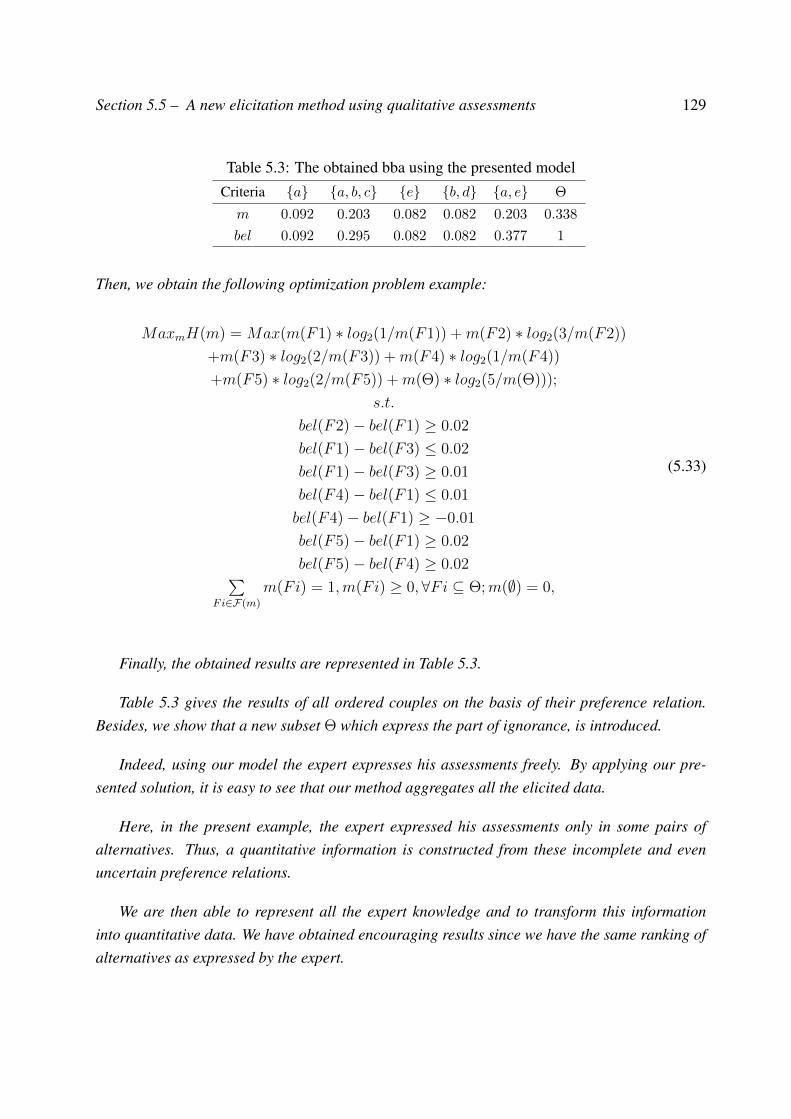
Section 5.5 – A new elicitation method using qualitative assessments 129
Table 5.3: The obtained bba using the presented modelCriteria a a, b, c e b, d a, e Θ
m 0.092 0.203 0.082 0.082 0.203 0.338
bel 0.092 0.295 0.082 0.082 0.377 1
Then, we obtain the following optimization problem example:
MaxmH(m) = Max(m(F1) ∗ log2(1/m(F1)) +m(F2) ∗ log2(3/m(F2))
+m(F3) ∗ log2(2/m(F3)) +m(F4) ∗ log2(1/m(F4))
+m(F5) ∗ log2(2/m(F5)) +m(Θ) ∗ log2(5/m(Θ)));
s.t.
bel(F2)− bel(F1) ≥ 0.02
bel(F1)− bel(F3) ≤ 0.02
bel(F1)− bel(F3) ≥ 0.01
bel(F4)− bel(F1) ≤ 0.01
bel(F4)− bel(F1) ≥ −0.01
bel(F5)− bel(F1) ≥ 0.02
bel(F5)− bel(F4) ≥ 0.02∑Fi∈F(m)
m(Fi) = 1,m(Fi) ≥ 0,∀Fi ⊆ Θ;m(∅) = 0,
(5.33)
Finally, the obtained results are represented in Table 5.3.
Table 5.3 gives the results of all ordered couples on the basis of their preference relation.Besides, we show that a new subset Θ which express the part of ignorance, is introduced.
Indeed, using our model the expert expresses his assessments freely. By applying our pre-sented solution, it is easy to see that our method aggregates all the elicited data.
Here, in the present example, the expert expressed his assessments only in some pairs ofalternatives. Thus, a quantitative information is constructed from these incomplete and evenuncertain preference relations.
We are then able to represent all the expert knowledge and to transform this informationinto quantitative data. We have obtained encouraging results since we have the same ranking ofalternatives as expressed by the expert.
Section 5.6 – Conclusion 130
5.5.4 A global model in the presence of different relations
After modeling the different preference relation, we propose to introduce a global model. Thismethod is concerned with preference models including: strict preference, weak preference, in-difference, incompleteness and incomparability:
MaxmUM(m)
s.t.
bel(a)− bel(b) ≥ γ ∀(a, b) for which a b
bel(a)− bel(b) ≤ γ ∀(a, b) for which a b
bel(a)− bel(b) ≥ ε ∀(a, b) for which a b
bel(a)− bel(b) ≤ ε ∀(a, b) for which a ∼ b
bel(a)− bel(b) ≥ −ε ∀(a, b) for which a ∼ b
bel(a) ≥ bel(b) ∀(a, b) for which a?b
pl(a) ≤ pl(b) ∀(a, b) for which a?b∑a∈F(m)
m(a) = 1;m(a) ≥ 0;∀a ⊆ Θ;m(∅) = 0
(5.34)
5.6 Conclusion
In this Chapter, a new model for constructing belief functions, that takes into account differentlevels of uncertainties, from elicited expert opinions has been defined. The originality of ourmodel is then to provide additional interpretation values to the existing methods.
In the following Chapter, we will focus on applying our proposed model in the multi-criteriadecision making field, which can be interesting in eliciting experts’ judgments.

Chapter 6AHP method based on beliefpreference relations
6.1 Introduction
Within the framework of AHP problems, a decision maker often needs to express his assessmentsusing crisp number. However, an expert may be uncertain about his level of preference due toincomplete information or knowledge, inherent complexity and uncertainty within the decisionenvironment. Thus, in such cases, the decision maker cannot estimate his assessments with anumerical value.
To overcome these difficulties, several AHP extensions were developed. However, theseapproaches deal only with numerical numbers to translate the expert preferences into quantitativeinformation.
To solve the problems presented above, and to facilitate the pair-wise comparison process,a new MCDM method under uncertainty that eliminates some of the drawbacks of the existingprioritization methods, is proposed. A natural way to cope with uncertain judgments is to expressthe comparison ratios as a belief function, which incorporates the imperfection of the humanthinking. Indeed, preferential assessments are used in order to express the decision maker’ssubjective assessments instead of using numerical values. Within our method, the expert does notrequire to complete all the comparison matrices; he can then derive priorities from incomplete set
131
Section 6.2 – On the extraction of scores from qualitative pair-wise comparison matrices 132
of judgments. Therefore, a new procedure is employed to derive crisp priorities from qualitativejudgments corresponding to each level.
In this Chapter, we give an insight into our proposed methods. We first give some motivationsto develop the qualitative AHP method for handling uncertainty. Then, we detail the proposedmethods and we give some examples to illustrate them.
6.2 On the extraction of scores from qualitative pair-wise com-parison matrices
Pair-wise comparisons aims at quantifying relative priorities for a given set of alternatives as wellas the set of criteria, on a ratio scale, based on the judgment of the decision maker. Using thisapproach, the decision maker has to express his opinion about the value of one single pair-wisecomparison at a time. Usually, he has to choose his answer among discrete choices. Each choiceis a linguistic phrase. Some examples of such linguistic phrases are: “A is more important thanB”, or “A is of the same importance as B”, or “A is a little more important than B”, and so on.Then, the decision maker uses the Saaty scale (see Table 1.4) to map the labels which indicatethe decision maker view to a numeric value.
However, as shown in Chapter 4, this scale was criticized. Moreover, using a quantitativescale, the expert cannot be consistent due to its inability to adequately handle the uncertaintyand imprecision associated with the mapping of the decision maker’s perception. For instance,he cannot estimate his degree of belief with a numerical value. Therefore, a new elicitationprocedure is introduced. In the proposed methodology, the expert is allowed to use preferencerelations only. Thus to express his judgments, the decision maker has to express his opinionsqualitatively, based on knowledge and experience that he provides in response to a given questionrather than direct quantitative information. He only selects the related linguistic variable usingpreference modeling.
For instance, to determine the criteria weights, the preference relation matrix is obtained (seeTable 6.1).
In this table, Pij is a preference relations. It may be:
1. a strict preference relation iff (ci cj) ∧ ¬(cj ci)

Section 6.2 – On the extraction of scores from qualitative pair-wise comparison matrices 133
Table 6.1: Preference relation matrixc1 c2 . . . cm
c1 - P12 . . . P1m
c2 - - . . . P2m
. . . - - - . . .cm - - - -
2. an indifference relation ∼ iff (ci cj) ∧ (cj ci)
3. a weak preference relation ((a, b) ∈ Q) iff (a b),
4. an unknown relation.
To complete the pair-wise matrix, the expert does not need to quantify his assessments and tofill all the pair-wise comparisons matrix. He is able to express his preferences freely. The experthas to complete only the matrix without quantifying the diagonal and the reciprocal matrix.
Example 6.1. To describe this approach, we consider the same problem of purchasing a car (Ex-ample 3.1). As we have already presented, this problem involves four criteria: Ω = Price (c1),
Style (c2), Fuel (c3), Reliability (c4) and three selected alternatives: Θ = Peugeot (p),Renault (r),
Ford (f). The expert has identified the following subsets of criteria c1, c4 and c2, c3.
Along with our qualitative pair-wise comparison process, the preference modeling defined inTable 6.2 was obtained.
Table 6.2: Preference relation matrix for criterion levelCriteria c1 c4 c2, c3c1 - c4 - - c2, c3 - - -
From this table, we conclude that the expert may say that c1 is evaluated to be more im-portant than c4 and c1 is evaluated to be more preferred than c2, c3.
Once the pair-wise comparison matrix is complete, our objective is then to obtain the priorityof each subset of element. In fact, within our model, we propose to transform these preference
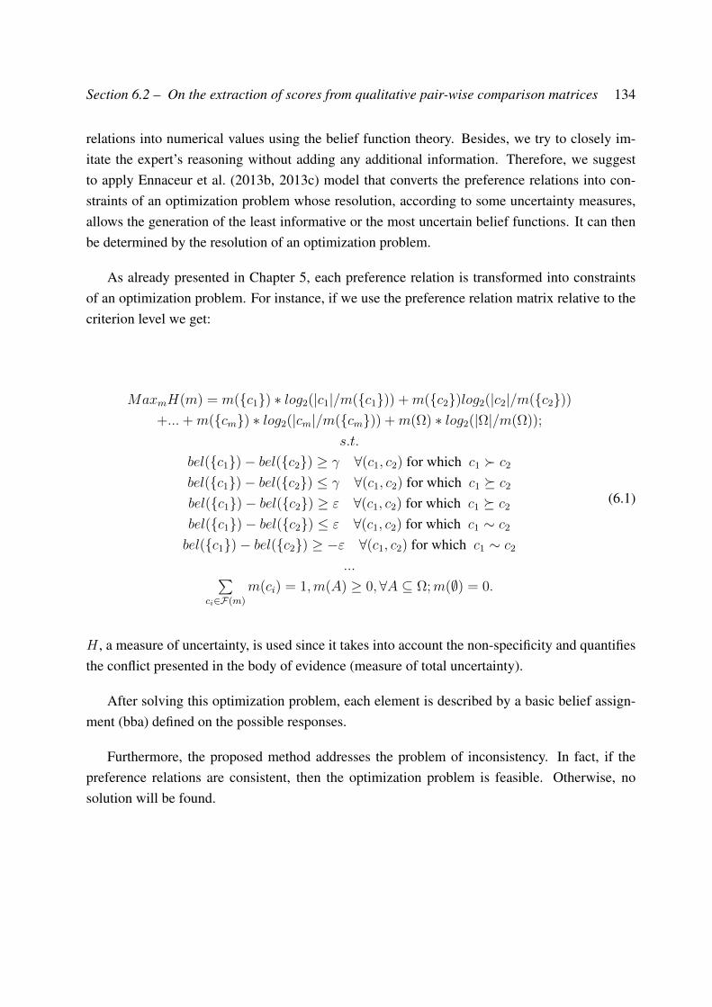
Section 6.2 – On the extraction of scores from qualitative pair-wise comparison matrices 134
relations into numerical values using the belief function theory. Besides, we try to closely im-itate the expert’s reasoning without adding any additional information. Therefore, we suggestto apply Ennaceur et al. (2013b, 2013c) model that converts the preference relations into con-straints of an optimization problem whose resolution, according to some uncertainty measures,allows the generation of the least informative or the most uncertain belief functions. It can thenbe determined by the resolution of an optimization problem.
As already presented in Chapter 5, each preference relation is transformed into constraintsof an optimization problem. For instance, if we use the preference relation matrix relative to thecriterion level we get:
MaxmH(m) = m(c1) ∗ log2(|c1|/m(c1)) +m(c2)log2(|c2|/m(c2))+...+m(cm) ∗ log2(|cm|/m(cm)) +m(Ω) ∗ log2(|Ω|/m(Ω));
s.t.
bel(c1)− bel(c2) ≥ γ ∀(c1, c2) for which c1 c2
bel(c1)− bel(c2) ≤ γ ∀(c1, c2) for which c1 c2
bel(c1)− bel(c2) ≥ ε ∀(c1, c2) for which c1 c2
bel(c1)− bel(c2) ≤ ε ∀(c1, c2) for which c1 ∼ c2
bel(c1)− bel(c2) ≥ −ε ∀(c1, c2) for which c1 ∼ c2
...∑ci∈F(m)
m(ci) = 1,m(A) ≥ 0,∀A ⊆ Ω;m(∅) = 0.
(6.1)
H , a measure of uncertainty, is used since it takes into account the non-specificity and quantifiesthe conflict presented in the body of evidence (measure of total uncertainty).
After solving this optimization problem, each element is described by a basic belief assign-ment (bba) defined on the possible responses.
Furthermore, the proposed method addresses the problem of inconsistency. In fact, if thepreference relations are consistent, then the optimization problem is feasible. Otherwise, nosolution will be found.
Section 6.3 – AHP method with belief preference relations 135
6.3 AHP method with belief preference relations
To handle uncertainty in the AHP method, we have first developed belief AHP method (Ennaceuret al., 2011), that deals with groups of criteria and alternatives and uses Saaty scale to modelexpert judgments. Then, we have studied the limit of this 1 − 9 scale and we have shown thatusing Saaty scale is not the most appropriate solution in some cases. This is because this scalecannot perfectly model the expert assessments in an uncertain environment. Therefore, we haveproposed a new AHP extension based on new set of choices, Yes-No/AHP approach.
On the other hand, we have shown in (Ennaceur et al., 2012a, 2013a, 2014b) that the experthas some difficulties in expressing his preferences using quantitative information. To solve thisissue, we have proposed new elicitation technique based on preference relations. In these works,we have shown that qualitative scale can perfectly model expert preferences.
Taking all these facts into consideration, we try to develop an overall MCDM method thatidentifies groups of criteria and alternatives and compares then using belief preference relations.
Let us remind that in the third Chapter of this dissertation, we have presented two AHP ex-tensions; namely belief AHP and conditional belief AHP. So to check the validity of our newelicitation technique, we will use our presented belief pair-wise comparisons with the aggrega-tion procedure adopted by these previously proposed methods. This leads us to develop twoAHP versions which we called qualitative AHP and conditional qualitative AHP. Details of thesealgorithms are given in the following Sections.
6.3.1 Qualitative AHP method
This Section is dedicated to the presentation of our new MCDM, called qualitative AHP method(Ennaceur et al., 2013b, 2013c). Indeed, our model has the same features as belief and Yes-No/AHP methods; however, it introduces a new pair-wise comparison technique. Nevertheless,we suggest to extend the belief AHP method under qualitative scale. A new aggregation proce-dure is then presented, as shown in Figure 6.1.
To present the qualitative AHP method, we introduce its different construction steps, de-scribed as follows.
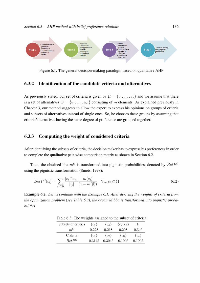
Section 6.3 – AHP method with belief preference relations 136
Figure 6.1: The general decision-making paradigm based on qualitative AHP
6.3.2 Identification of the candidate criteria and alternatives
As previously stated, our set of criteria is given by Ω = c1, . . . , cn and we assume that thereis a set of alternatives Θ = a1, . . . , am consisting of m elements. As explained previously inChapter 3, our method suggests to allow the expert to express his opinions on groups of criteriaand subsets of alternatives instead of single ones. So, he chooses these groups by assuming thatcriteria/alternatives having the same degree of preference are grouped together.
6.3.3 Computing the weight of considered criteria
After identifying the subsets of criteria, the decision maker has to express his preferences in orderto complete the qualitative pair-wise comparison matrix as shown in Section 6.2.
Then, the obtained bba mΩ is transformed into pignistic probabilities, denoted by BetPΩ
using the pignistic transformation (Smets, 1998):
BetPΩ(ci) =∑cj⊆Θ
|ci ∩ cj||cj|
m(cj)
(1−m(∅)), ∀ci, ci ⊂ Ω (6.2)
Example 6.2. Let us continue with the Example 6.1. After deriving the weights of criteria fromthe optimization problem (see Table 6.3), the obtained bba is transformed into pignistic proba-bilities.
Table 6.3: The weights assigned to the subset of criteriaSubsets of criteria c1 c4 c2, c3 Ω
mΩ 0.228 0.218 0.208 0.346
Criteria c1 c2 c3 c4BetPΩ 0.3145 0.3045 0.1905 0.1905
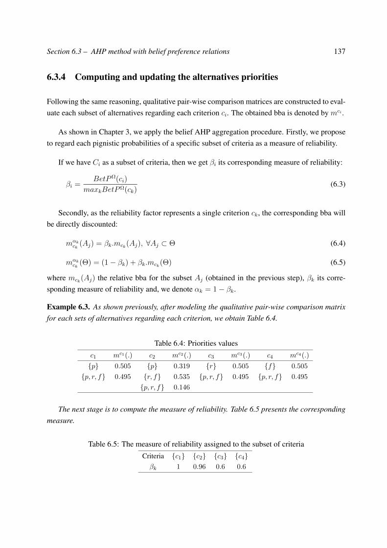
Section 6.3 – AHP method with belief preference relations 137
6.3.4 Computing and updating the alternatives priorities
Following the same reasoning, qualitative pair-wise comparison matrices are constructed to eval-uate each subset of alternatives regarding each criterion ci. The obtained bba is denoted by mci .
As shown in Chapter 3, we apply the belief AHP aggregation procedure. Firstly, we proposeto regard each pignistic probabilities of a specific subset of criteria as a measure of reliability.
If we have Ci as a subset of criteria, then we get βi its corresponding measure of reliability:
βi =BetPΩ(ci)
maxkBetPΩ(ck)(6.3)
Secondly, as the reliability factor represents a single criterion ck, the corresponding bba willbe directly discounted:
mαkck
(Aj) = βk.mck(Aj), ∀Aj ⊂ Θ (6.4)
mαkck
(Θ) = (1− βk) + βk.mck(Θ) (6.5)
where mck(Aj) the relative bba for the subset Aj (obtained in the previous step), βk its corre-sponding measure of reliability and, we denote αk = 1− βk.
Example 6.3. As shown previously, after modeling the qualitative pair-wise comparison matrixfor each sets of alternatives regarding each criterion, we obtain Table 6.4.
Table 6.4: Priorities valuesc1 mc1(.) c2 mc2(.) c3 mc3(.) c4 mc4(.)
p 0.505 p 0.319 r 0.505 f 0.505
p, r, f 0.495 r, f 0.535 p, r, f 0.495 p, r, f 0.495
p, r, f 0.146
The next stage is to compute the measure of reliability. Table 6.5 presents the correspondingmeasure.
Table 6.5: The measure of reliability assigned to the subset of criteriaCriteria c1 c2 c3 c4βk 1 0.96 0.6 0.6
Section 6.3 – AHP method with belief preference relations 138
After computing the belief functions for each set of alternatives with respect to each criterion,we need to combine the weight of criteria and the alternatives priorities. Table 6.6 defines thediscounted bbas.
Table 6.6: The discounted bbasc1 mα1
c1 (.) c2 mα2c2 (.) c3 mα3
c3 (.) c4 mαkc4 (.)
p 0.505 p 0.1914 r 0.303 f 0.4848
p, r, f 0.495 r, f 0.321 p, r, f 0.697 p, r, f 0.5152
p, r, f 0.4876
6.3.5 Decision making
To this end and after updating the relative bba, a decision under uncertainty must be defined. Inthe sequel, the pignistic probabilities are used. Therefore, our obtained beliefs must be combined.To do so, we propose to apply the conjunctive rule:
mfinal = ∩©mαkck, k = 1, . . . , n (6.6)
Now, we can compute the pignistic probabilities to choose the best alternatives.
Example 6.4. Let us continue with the previous example and remind that our objective is to rankalternative in an uncertain environment. Hence, our first stage is to combine the overall bbas.The obtained result is illustrated in Table 6.7.
Table 6.7: The overall bba∅ p r r, f Θ
mfinal 0.4072 0.3866 0.06248 0.0570 0.0867
Finally, the ranking of alternative is obtained according to the pignistic transformation (seeTable 6.8).
Section 6.4 – Introducing dependency under qualitative AHP method: Conditional qualitative AHP139
Table 6.8: The final result using the Yes-No/AHP approachAlternatives p r f
BetP 0.70088 0.20226 0.096861
6.4 Introducing dependency under qualitative AHP method:Conditional qualitative AHP
As we have presented previously in Chapter 3, we need to model the relationship between alter-natives and criteria. Thus, in this Section, our main objective is to handle dependency betweenthe two levels under the qualitative AHP methodology. Besides, we propose the latter by us-ing preference relation in order to translate the expert’s assessments. Figure 6.2 summarizes thecomputational procedure.
Figure 6.2: The general decision-making paradigm based on conditional qualitative AHP
From Figure 6.2, the major difference between conditional qualitative AHP and other AHPextensions is in Step 2. So, our solution proposes to use preferential judgments instead of Saatyscale. Therefore, the following stages must be respected (Ennaceur et al., 2014c):
1. Identification of the sets of criteria and groups of alternatives.
2. The criterion level is described by the obtained bba using preference relations.
3. At the alternative level, each pair-wise comparison matrix is constructed using preferencerelations and the obtained bba is described by conditional beliefs.
4. Standardizing the frame of discernment. At the criterion level, the vacuous extension isused. At the alternative level, we apply the ballooning extension technique.
5. The conjunctive rule is defined to combine the overall bbas.
6. Decision making using pignistic transformation.

Section 6.5 – Experimental analysis 140
6.5 Experimental analysis
To test the validity of our developed methods, our experiments are performed on the same randomdata sets presented in Chapter 3.
6.5.1 Simulation algorithm
Despite the possible differences between the obtained results through three MCDM methods, wecannot conclude the superiority of one over another. Unless we have a solid basis, we comparethe ranking results against the closeness of the rankings of each method to the actual rankings.To do so, we need to compare each set of rankings provided by AHP and the proposed methodswith a ranking that has been already produced by an alternative, yet reliable ranking method.This alternative ranking will be considered as a basis, or actual ranking of the alternatives andwill be used to measure the closeness of the rankings provided by AHP, qualitative AHP andconditional qualitative AHP to reality.
In order to overcome these issues, in the next Section, we test a simulation algorithm thatcompares the ranking results of the three methods under different scenarios.
To generate reliable data for a numerical analysis, we have applied the following algorithm:
1. We generate a random matrix for the decision performance as well as a random matrix torepresent the weight of each decision criteria. Based on these two matrices, the overallscores and ranks of the decision alternatives are calculated. These are usual steps in theWSM method.
2. From the performance matrix, we generated pair-wise comparison matrices of differentalternatives that are compared to each criterion.
3. Each pair-wise comparison matrix is transformed into qualitative assessment using pref-erence relations. The qualitative matrix of the actual pair-wise comparisons would beobtained as follows:
• “Equal importance” is equivalent to indifference relation.
• “Somewhat more important” and “Much more important” are equivalent to weakpreference relation.
Section 6.5 – Experimental analysis 141
• “Very much more important” and “Absolutely more important” are equivalent tostrong preference relation.
4. We apply the suggested method to compute the overall priorities and to rank alternatives.
5. We compare the obtained result with the ranking of the WSM method.
Let’s demonstrate the evaluation procedure using the same example 3.10 introduced in Chapeter3. We consider 3 alternatives a1, a2 and a3 and three criteria c1, c2 and c3. The decision makingproblem is described using the matrix presented in Table 6.9.
Table 6.9: Decision matrixCriteria
c1 c2 c3
813
213
313
a1 1 9 9
a2 5 2 2
a3 1 5 9
This example has been solved using the WSM and AHP in (Triantaphyllou & Mann, 1989).While applying the WSM, it can be shown that the alternative a1 is the best one. However, AHPturns out that the alternative a2 is the best. Obviously, this is in contradiction with the conclusionderived using the WSM.
Now, let us model this example using qualitative AHP. As a result, the pair-wise comparisonmatrix of the three alternatives in terms of each criterion is illustrated in Table 6.10.
Next, an optimization model is used to transform preference relation into constraints andto generate quantitative information from these qualitative assessments. Finally, we obtain the
Table 6.10: The preference relations matrices
c1
a1 a2 a3
a1 - ≺ ∼a2 - - a3 - - -
c2
a1 a2 a3
a1 - ∼a2 - - ∼a3 - - -
c3
a1 a2 a3
a1 - ∼a2 - - ∼a3 - - -

Section 6.5 – Experimental analysis 142
following order: a1 a3 a2. Obviously, this is in contradiction with the results derived whenthe AHP method was applied at the beginning of this illustrative example. However, we haveobtained encouraging results since it can be observed that the ranking order of the alternatives asderived by the WSM and the qualitative AHP is the same.
In order to gain a deeper understanding, a computational study was undertaken. The datawere random numbers from the interval [1, 9]. In these test problems, the number of alternativeswas equal to the following values: 3, 4, 5, 6, 7, 8, 9 and 10. Similarly, the number of criteria wasequal to 3, 4, 5, 6, 7, 8, 9 and 10. Test problems were treated as the previous illustrative example.Any ranking irregularity was recorded.
6.5.2 Simulation results
Let us reiterate the immediate goal of this Section: We wish to check the accuracy of our pro-posed models by comparing them to WSM method.
Figure 6.3: Percentage of contradiction (%) based on 3 alternatives
From Figures 6.3 and 6.4, our qualitative AHP achieves a satisfactory percentage of contra-diction when it is compared regarding a few numbers of alternatives and criteria. Indeed, wehave to point out that our two methods, qualitative AHP and conditional qualitative AHP, givethe lowest percentage of contradiction in almost the cases in comparison to the other presentedmethods (see Chapters 3 and 4). This can be explained by the appropriate use of the preferencerelations to model expert assessments.
The qualitative AHP methods perform much better than standard AHP on the whole. For in-
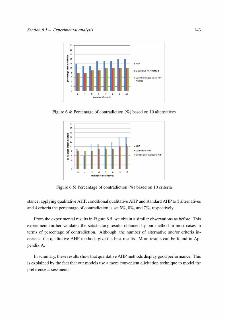
Section 6.5 – Experimental analysis 143
Figure 6.4: Percentage of contradiction (%) based on 10 alternatives
Figure 6.5: Percentage of contradiction (%) based on 10 criteria
stance, applying qualitative AHP, conditional qualitative AHP and standard AHP to 3 alternativesand 4 criteria the percentage of contradiction is set 5%, 5%, and 7%, respectively.
From the experimental results in Figure 6.5, we obtain a similar observations as before. Thisexperiment further validates the satisfactory results obtained by our method in most cases interms of percentage of contradiction. Although, the number of alternative and/or criteria in-creases, the qualitative AHP methods give the best results. More results can be found in Ap-pendix A.
In summary, these results show that qualitative AHP methods display good performance. Thisis explained by the fact that our models use a more convenient elicitation technique to model thepreference assessments.

Section 6.5 – Experimental analysis 144
Yet, it is important to mention that the main conclusion from the works presented in Ennaceuret al. (2011, 2012b, 2014a), detailed in Chapter 3 and Chapter 4, and Ennaceur et al. (2013b,2013c, 2014c) are, also, described in this Chapter, is the superiority of qualitative AHP ap-proaches comparing to the studied methods. This is because the method is able to model expertpreferences adequately using only belief preference relations. Consequently, in the followingSection, we will check the consistency of the presented methodologies.
6.5.3 Catering selection problem
Figures 6.6 and 6.7 show a sensitivity analysis between the qualitative AHP method and condi-tional qualitative AHP version. Focusing on the consistency of the methods, Table 6.11 showsthe obtained ranking.
Figure 6.6: Sensitivity analysis of Hygiene criterion
Table 6.11: Decision matrixAlt. Ranking
Qualitative AHP Condtional qualitative AHPDurusu 0.34 0.23
Mertol 0.29 0.18
Afiyetle 0.37 0.59
Firstly, consider the Hygiene criterion. By increasing the share of this latter, it has beennoticed that the model is still in favor of Afiyetle with a score followed by Durusu and lastly
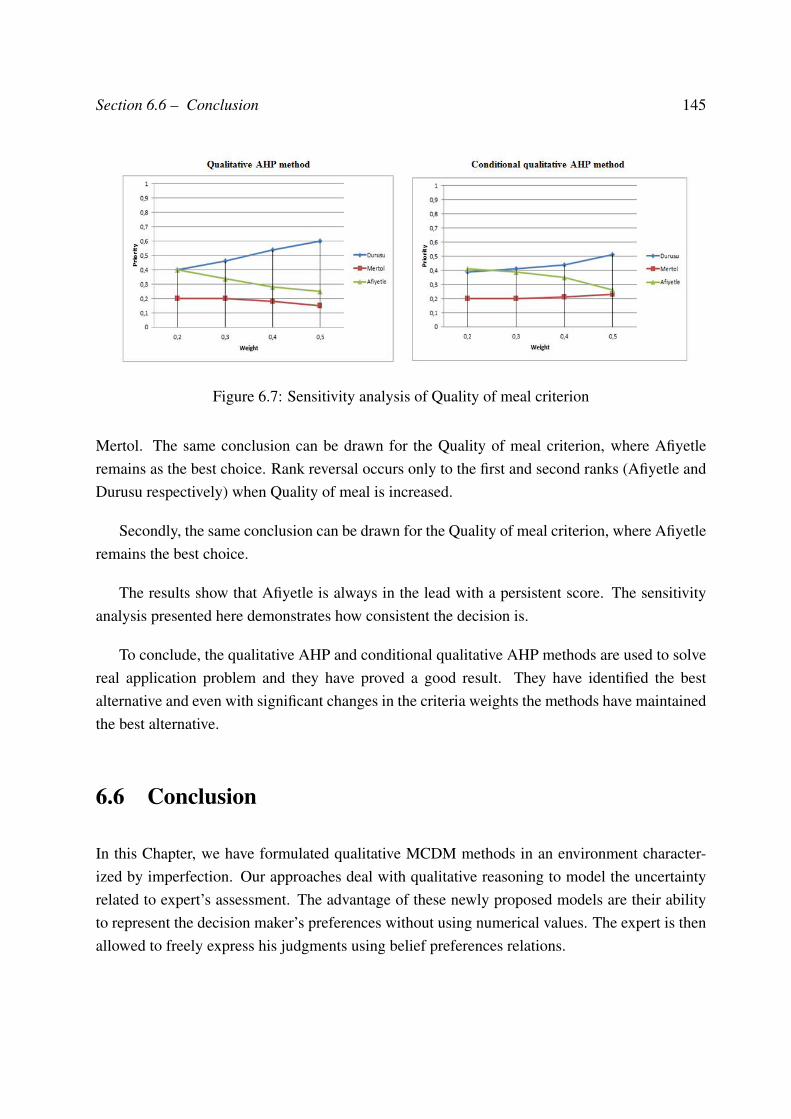
Section 6.6 – Conclusion 145
Figure 6.7: Sensitivity analysis of Quality of meal criterion
Mertol. The same conclusion can be drawn for the Quality of meal criterion, where Afiyetleremains as the best choice. Rank reversal occurs only to the first and second ranks (Afiyetle andDurusu respectively) when Quality of meal is increased.
Secondly, the same conclusion can be drawn for the Quality of meal criterion, where Afiyetleremains the best choice.
The results show that Afiyetle is always in the lead with a persistent score. The sensitivityanalysis presented here demonstrates how consistent the decision is.
To conclude, the qualitative AHP and conditional qualitative AHP methods are used to solvereal application problem and they have proved a good result. They have identified the bestalternative and even with significant changes in the criteria weights the methods have maintainedthe best alternative.
6.6 Conclusion
In this Chapter, we have formulated qualitative MCDM methods in an environment character-ized by imperfection. Our approaches deal with qualitative reasoning to model the uncertaintyrelated to expert’s assessment. The advantage of these newly proposed models are their abilityto represent the decision maker’s preferences without using numerical values. The expert is thenallowed to freely express his judgments using belief preferences relations.

Conclusion
This PhD Thesis was devoted to the modelling of uncertainty under the AHP method. Uncer-tainty is formalized using the belief function framework.
In real-life decision making situation, the decision maker may encounter several difficultieswhen expressing his own level of preferences between alternatives or also criteria. However,standard version of AHP method is not adapted to ensure its role in such environment. Thus, theneed of the development of appropriate approach to this kind of environment is vital.
For that reason, as a first contribution, we have revised the theoretical aspects of AHP methodand we have proposed a new belief AHP method. When building the AHP hierarchy, our newapproach uses subsets of criteria and alternatives instead of singletons, in order to reduce thenumber of comparisons. So, the expert has to express his knowledge to alternatives and criteriawhich he has a level of opinion towards.
Another main contribution of this PhD Thesis is to model the dependency between the alter-natives and criteria. Consequently, we have been focused on representing the influences of thecriteria on the evaluation of alternatives. In this latter, uncertainty is given in terms of conditionalmass distributions. While making a decision, we need to allow for both and not to take the simpleway out by always assuming independency.
The last part of the work provides some criticisms according to the comparison procedure.In fact, we have extended the belief AHP approach on a more flexible method by introducinguncertainty in the pair-wise comparison matrix. Thus, to evaluate the responses of the pair-wise comparison question, the decision maker expresses his judgment with some degrees ofuncertainty.
147

Conclusion 148
Focusing on this aspect, we have proposed two different AHP extensions: Yes-No/AHP andqualitative AHP. The first expert judgment elicitation method is based on mass distributions,while the second one is based on preference relations. These introduced methods could producesignificantly better results than standard AHP. Besides, using the first model, the uncertaintymay appear in pair-wise comparisons values and is represented by bbas notion. This approachallows the expert to model his ignorance and to represent his imperfection. Despite of the ad-vantages of the developed Yes-No/AHP method, the decision maker needs to quantify his degreeof preferences. To handle this limitation, qualitative AHP approach has been developed. Thismethodology uses preference relations to model expert judgments. As a result, this qualitativeAHP method is advantageous over the other proposed techniques.
While developing our qualitative AHP method, we have noticed that we need to introduce anew model that generates quantitative information from qualitative assessment. For this reason,we have proposed a new expert judgment elicitation method under the belief function frameworkthat produces quantitative mass distributions from preference relations. The originality of ourmodel is its ability to model different preference levels and to generate quantitative informationfrom qualitative one only.
Finally, the performances of the proposed methods and the other approaches are comparedaccording to the defined performance measure. In the computational experiments, the proposedYes-No/AHP and qualitative AHP methods showed the best performances in all of the randomlygenerated matrices. When these two methods are compared, the second variation showed a betterperformance as the dimension of the matrices increases. Also, we have checked the robustnessand the stability of the developed methods for maintaining the best solution. Applying sensitivityanalysis to catering selection problem is essential to ensure the consistency of final decision.
In summary, the whole work is presented by Figure 6.8 which shows the main characteristicsof the proposed methods.
Nevertheless, there exists a certain amount of problems which cannot be solved by standardAHP framework. With this work, we have been able to show that the way of solving a decisionproblem depends on the available information, on the objectives, on the possible and potentialinteractions with the decision maker and on the type of process which is eligible.
Some interesting future works have to be mentioned. First, in some situations, the decisionmaker may be a group or an organization. An application of the proposed method to the groupdecision making situations can then be done. We can, also, be interested in studying more com-
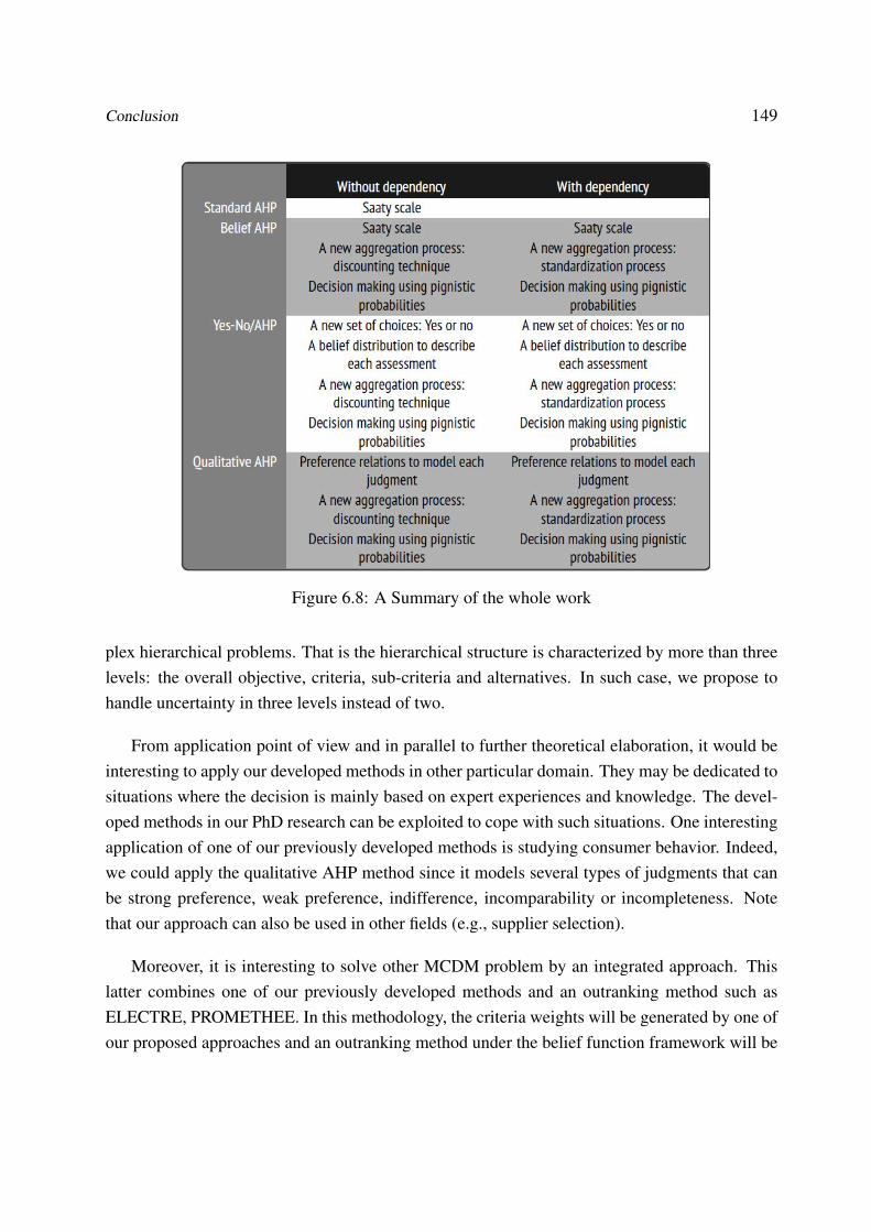
Conclusion 149
Figure 6.8: A Summary of the whole work
plex hierarchical problems. That is the hierarchical structure is characterized by more than threelevels: the overall objective, criteria, sub-criteria and alternatives. In such case, we propose tohandle uncertainty in three levels instead of two.
From application point of view and in parallel to further theoretical elaboration, it would beinteresting to apply our developed methods in other particular domain. They may be dedicated tosituations where the decision is mainly based on expert experiences and knowledge. The devel-oped methods in our PhD research can be exploited to cope with such situations. One interestingapplication of one of our previously developed methods is studying consumer behavior. Indeed,we could apply the qualitative AHP method since it models several types of judgments that canbe strong preference, weak preference, indifference, incomparability or incompleteness. Notethat our approach can also be used in other fields (e.g., supplier selection).
Moreover, it is interesting to solve other MCDM problem by an integrated approach. Thislatter combines one of our previously developed methods and an outranking method such asELECTRE, PROMETHEE. In this methodology, the criteria weights will be generated by one ofour proposed approaches and an outranking method under the belief function framework will be
Conclusion 150
employed to assess different alternatives under uncertainty.
Another line of research could be the integration of machine learning methods in decisionanalysis. The decision process has two major aims: first, to explain decisions and second, to giverecommendations: how to make a decision under specific circumstances. These are very similarto the goals of the machine learning approach, where the first step is to establish a model fromprevious experience which is then applied to predict future situations. This parallelism leads tothe application of these methods in decision making. Therefore, it will be useful to study howthese two fields can interact and how they can handle uncertainty in their parameters.
For instance, in a problem of credit scoring, one of its most important parts is determiningthe class of customers to run a classification algorithm. The purpose of this research will be theallocation of the labels of credit customers using one of the developed AHP methods. Here, in thefirst step, each customer will be labeled by an AHP extension and then a classification algorithmwill be applied. In this way, via this method the acquired results of data mining algorithms couldbe improved.

Appendix AExperimental results
A.1 Introduction
In this Appendix, all the experimental results will be given. To test the validity of our proposedmodels, our experiments are performed on the same generated data as described in the previousChapters. We will show that some methods are better than others in some cases even thoughnone of the methods is perfectly accurate.
A.2 Experimental analysis
In this Section, we present the results of our simulation study using AHP, belief AHP, conditionalbelief AHP, Yes-No/AHP, conditional Yes-No/AHP, qualitative AHP and conditional qualitativeAHP methods.
152
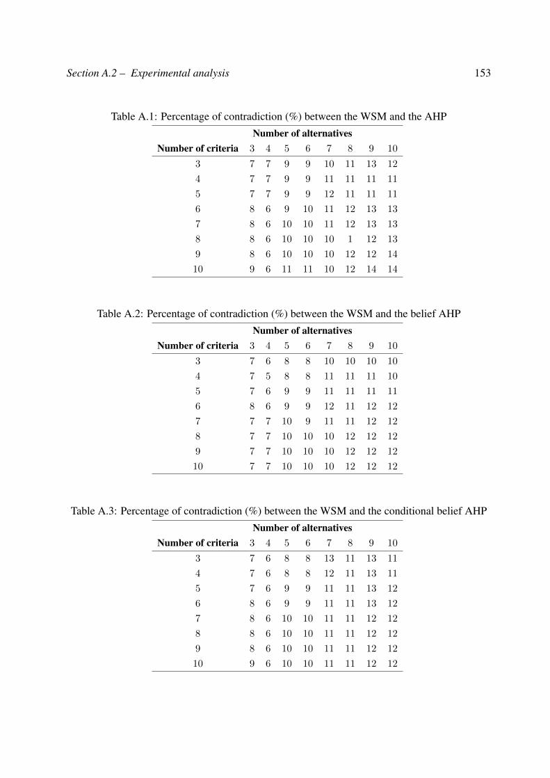
Section A.2 – Experimental analysis 153
Table A.1: Percentage of contradiction (%) between the WSM and the AHPNumber of alternatives
Number of criteria 3 4 5 6 7 8 9 10
3 7 7 9 9 10 11 13 12
4 7 7 9 9 11 11 11 11
5 7 7 9 9 12 11 11 11
6 8 6 9 10 11 12 13 13
7 8 6 10 10 11 12 13 13
8 8 6 10 10 10 1 12 13
9 8 6 10 10 10 12 12 14
10 9 6 11 11 10 12 14 14
Table A.2: Percentage of contradiction (%) between the WSM and the belief AHPNumber of alternatives
Number of criteria 3 4 5 6 7 8 9 10
3 7 6 8 8 10 10 10 10
4 7 5 8 8 11 11 11 10
5 7 6 9 9 11 11 11 11
6 8 6 9 9 12 11 12 12
7 7 7 10 9 11 11 12 12
8 7 7 10 10 10 12 12 12
9 7 7 10 10 10 12 12 12
10 7 7 10 10 10 12 12 12
Table A.3: Percentage of contradiction (%) between the WSM and the conditional belief AHPNumber of alternatives
Number of criteria 3 4 5 6 7 8 9 10
3 7 6 8 8 13 11 13 11
4 7 6 8 8 12 11 13 11
5 7 6 9 9 11 11 13 12
6 8 6 9 9 11 11 13 12
7 8 6 10 10 11 11 12 12
8 8 6 10 10 11 11 12 12
9 8 6 10 10 11 11 12 12
10 9 6 10 10 11 11 12 12
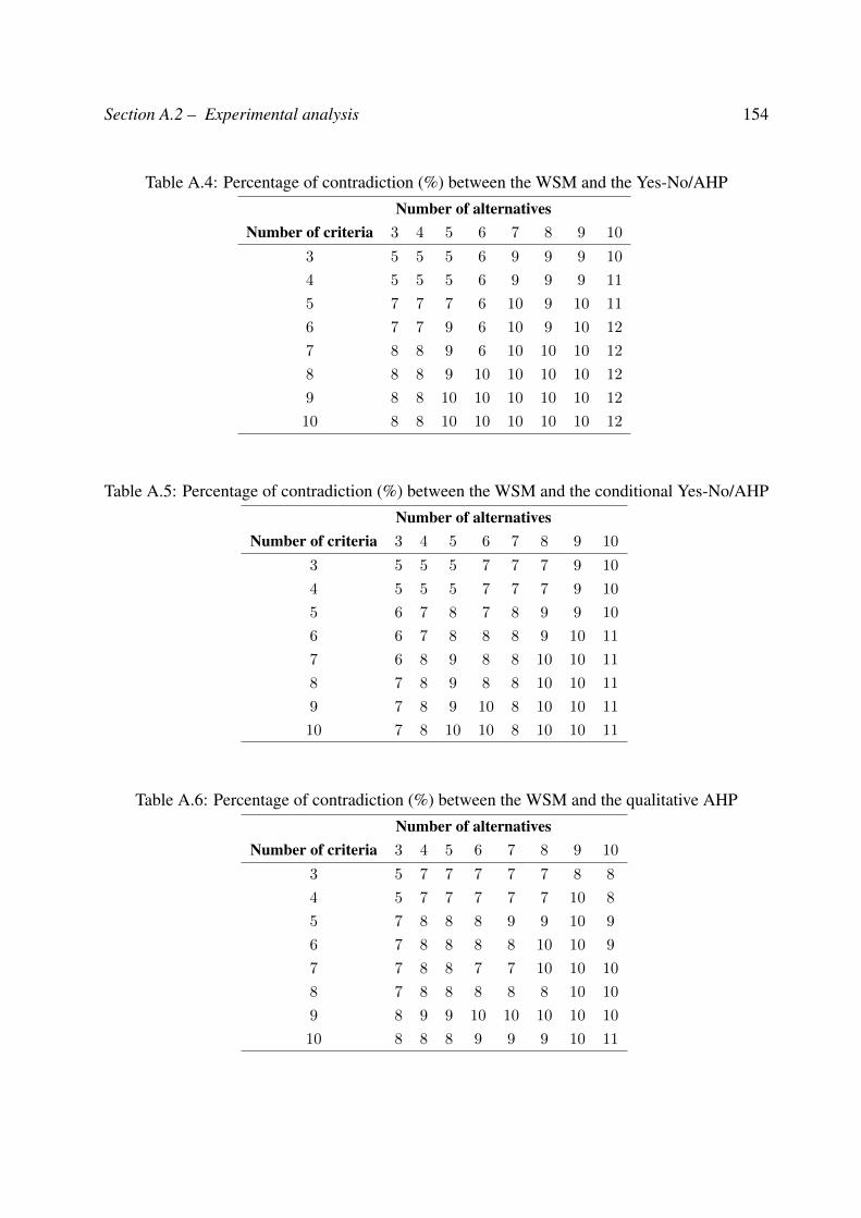
Section A.2 – Experimental analysis 154
Table A.4: Percentage of contradiction (%) between the WSM and the Yes-No/AHPNumber of alternatives
Number of criteria 3 4 5 6 7 8 9 10
3 5 5 5 6 9 9 9 10
4 5 5 5 6 9 9 9 11
5 7 7 7 6 10 9 10 11
6 7 7 9 6 10 9 10 12
7 8 8 9 6 10 10 10 12
8 8 8 9 10 10 10 10 12
9 8 8 10 10 10 10 10 12
10 8 8 10 10 10 10 10 12
Table A.5: Percentage of contradiction (%) between the WSM and the conditional Yes-No/AHPNumber of alternatives
Number of criteria 3 4 5 6 7 8 9 10
3 5 5 5 7 7 7 9 10
4 5 5 5 7 7 7 9 10
5 6 7 8 7 8 9 9 10
6 6 7 8 8 8 9 10 11
7 6 8 9 8 8 10 10 11
8 7 8 9 8 8 10 10 11
9 7 8 9 10 8 10 10 11
10 7 8 10 10 8 10 10 11
Table A.6: Percentage of contradiction (%) between the WSM and the qualitative AHPNumber of alternatives
Number of criteria 3 4 5 6 7 8 9 10
3 5 7 7 7 7 7 8 8
4 5 7 7 7 7 7 10 8
5 7 8 8 8 9 9 10 9
6 7 8 8 8 8 10 10 9
7 7 8 8 7 7 10 10 10
8 7 8 8 8 8 8 10 10
9 8 9 9 10 10 10 10 10
10 8 8 8 9 9 9 10 11

Section A.3 – Conclusion 155
Table A.7: Percentage of contradiction (%) between the WSM and the conditional qualitativeAHP
Number of alternativesNumber of criteria 3 4 5 6 7 8 9 10
3 5 7 7 7 7 7 8 8
4 5 7 7 7 7 7 10 8
5 5 8 8 8 9 9 10 9
6 6 8 8 9 9 10 10 9
7 6 8 8 9 9 9 10 10
8 6 8 8 9 9 9 10 10
9 8 9 9 10 10 10 10 10
10 8 8 8 9 9 9 10 10
A.3 Conclusion
In this Appendix, we have elucidated the different results obtained using the different developedapproaches.
Appendix BSensitivity analysis
B.1 Introduction
The objective of this Appendix is to briefly review typical sensitivity analysis methods and torecommend the selection of method to study the case of catering selection problem. Sensitivityanalysis methods may be broadly classified as mathematical methods, statistical (or probabilis-tic) methods, and graphical methods. This classification helps in understanding applicability ofsensitivity analysis methods for different types of models, and in selecting appropriate methodsaccording to their usefulness to a decision maker.
Mathematical methods are useful for deterministic and probabilistic models. Statistical meth-ods are generally used for probabilistic models. Graphical methods can be used for any kind ofmodel (Frey & Patil, 2002).
In Section B.2, the basics of mathematical methods will be given. In Section B.3, the mainnotions of the statistical methods will be introduced while in Section B.4, the fundamental no-tions graphical methods will be highlighted.
156
Section B.2 – Mathematical methods 157
B.2 Mathematical methods
This group of sensitivity analysis methods uses mathematical models when it is possible to ex-press the relationship between the input data and the problem solution. Mathematical modelshave better performance and are the most efficient as they do not require iteration. Moreover,their results are much more accurate when using verified formulas. Many works have been pre-sented such as: (Frey & Patil, 1990), (Huang, 1990) and (Erkut & Tarimcilar, 1991).
Several authors have developed mathematical models for sensitivity analysis in AHP. Freyand Patil (1990) studied how changes throughout the whole domain in the weights of criteriamay affect the ranking of alternatives and proposed a sensitivity coefficient representing thepossibility of rank reversal from these changes.
Huang (1990) found an inconsistency in Masudas coefficient as a large value of the coefficientmay not necessarily mean that a rank reversal will occur, and vice versa, a low value of thecoefficient may produce a rank reversal. To overcome this, Huang proposed a new sensitivitycoefficient and demonstrated it reveals the sensitivity of an AHP model with more accuracy thanMasuda’s coefficient.
Erkut and Tarimcilar (1991) presented a method to analyze and visualize in the weight spacethe ranking of alternatives with respect to all possible combinations of weights for the first levelof criteria. The method works by partitioning the weight space into n subsets, where n is thenumber of criteria. However, there are limitations in their method. It does not provide a methodfor performing sensitivity analysis when the problem has more than one level of criteria. More-over, if more than three criteria are simultaneously considered, then visual representation is notpossible and the weight space is no longer a triangle, it becomes a convex polyhedron.
B.3 Statistical methods
Simulation methods replace judgments in the pair-wise comparison matrix with values fromprobability distributions and perform a number of simulations to calculate the expected rankingof alternatives. As probabilistic input is used, the problem is no longer deterministic. Thisapproach allows for changing more than one parameter at a time.
Section B.4 – Graphical methods 158
Statistical methods are widely used for probabilistic models as these methods can evaluatethe effect of variance in the inputs on the output. A probabilistic model is itself deterministic innature, but inputs are assigned distributions (Frey & Patil, 2002).
Butler et al. (1997) proposed a method using Monte-Carlo simulations that allows randomchange of all weights simultaneously to explore the effect on the ranking. They presented threetypes of simulations:
• Random weights: All criteria weights are generated completely at random in order todiscover how the ranking of the alternatives changes under any conditions.
• Random weights preserving rank order: If the ranking of criteria weights are of importanceand have to be preserved, then the procedure is similar to the previous one with the differ-ence that the random weights are ranked according to the original criteria ranking and thenare used to calculate the solution.
• Random weights from a response distribution: This type of simulation considers the cur-rent weights as means of probability distributions and the random weights for the simula-tion are generated from these distributions.
B.4 Graphical methods
This approach involves changing the weight values and calculating the new solution. The method,also known as One-at-a-time (OAT), works by incrementally changing one parameter at a time,calculating the new solution and graphically presenting how the global ranking of alternativeschanges. This is the most popular in the literature where AHP is used to solve problems.
Graphical methods give representation of sensitivity in the form of graphs, charts, or surfaces.Generally, they are used to give a visual indication of how an output is affected by variation ininputs. Also, they can be used as a screening method before further analysis of a model or torepresent complex dependencies between inputs and outputs.
Graphical methods can be used to complement the results of mathematical and statisticalmethods for better interpretation.
Section B.5 – Conclusion 159
B.5 Conclusion
This Appendix has presented a discussion of sensitivity analysis was presented and its differenttypes were covered.
Sensitivity analysis methods may be grouped into three main categories: graphical methods,probabilistic simulations and mathematical models. The first method is the most popular becauseof its simplicity and easy implementation. Therefore, in this work, we have use it as a sensitivityanalysis technique. However, the other two groups of methods may provide more insights on adecision problem as they allow simultaneous analysis on more than one decision element.
References
Arbel, A. (1989). Approximate articulation of preference and priority derivation. EuropeanJournal of Operational Rerearch, 43, 317–327.
Belton, V., & Gear, A. (1983). On a shortcoming of Saaty’s method of analytic hierarchies.OMEGA, 11(3), 227–230.
Belton, V., & Stewart, T. J. (2003). Multiple Criteria Decision Analysis: an integrated approach.Kluwer Academic Publishers.
Ben Yaghlane, A., Denoeux, T., & Mellouli, K. (2006). Constructing belief functions from expertopinions. Proceedings of the 2nd International Conference on Information and Communi-cation Technologies: from Theory to Applications (ICTTA 2006), Damascus, Syria, 75-89.
Beynon, M. (2002a). An analysis of distributions of priority values from alternative comparisonscales within AHP. European Journal of Operational Research, 140, 105-118.
Beynon, M. (2002b). DS/AHP method: A mathematical analysis, including an understanding ofuncertainty. European Journal of Operational Research, 140, 148–164.
Beynon, M., Curry, B., & Morgan, P. (2000). The Dempster-Shafer theory of evidence: Analternative approach to multicriteria decision modelling. OMEGA, 28(1), 37–50.
Beynon, M., Xu, D. C., & Marshall, D. (2001). An expert system for Multi-Criteria DecisionMaking using Dempster Shafer theory. Expert Systems with Applications, 20, 357–367.
Boujelben, M. A., Smet, Y. D., Frikha, A., & Chabchoub, H. (2011). A ranking model inuncertain, imprecise and multi-experts contexts: The application of evidence theory. In-ternational Journal of Approximate Reasoning, 52, 1171-1194.
Bouyssou, D., & Vincke, P. (2009). Binary relations and preference modeling, in decision-making process: Concepts and methods. (eds D. Bouyssou, D. Dubois, M. Pirlot and H.Prade), ISTE, London, UK.
Bryson, N., & Mobolurin, A. (1999). A process for generating quantitative belief functions.
160
References 161
European Journal of Operational Research, 115, 624-633.Buckley, J. J. (1985). Fuzzy hierarchical analysis. Fuzzy Sets and Systems, 17, 233–247.Butler, J., Jia, J., & Dyer, J. (1997). Simulation techniques for the sensitivity analysis of multi-
criteria decision models. European Journal of Operational Research, 103(3), 531–546.Cebeci, U., & Kahraman, C. (2002). Measuring customer satisfaction of catering service com-
panies using fuzzy AHP: The case of Turkey. Proceedings of International Conference onFuzzy Systems and Soft Computational Intelligence in Management and Industrial Engi-neering, Istanbul, 315-325.
Chamodrakas, I., Batis, D., & Martakos, D. (2010). Supplier selection in electronic marketplacesusing satisficing and fuzzy AHP. Expert Systems with Applications, 37, 490-498.
Chang, D. Y. (1996). Applications of the extent analysis method on fuzzy AHP. EuropeanJournal of Operation Research, 95, 649–655.
Costa, C. A. B. E., & Vansnick, J. C. (1994). MACBETH: An interactive path towards the con-struction of cardinal value function. International Transactions in Operational Research,1(4), 489–500.
Creed, P. (2001). The potential of foodservice systems for satisfying consumer needs. InnovativeFood Science and Emerging Technologies, 2, 219-227.
Debreu, G. (1959). Theory of value: An axiomatic analysis of economic equilibrium. JohnWiley and Sons Inc., New York.
Dempster, A. (1967). Upper and lower probabilities induced by a multiple valued mapping.Annals of Mathematical Statistics, 38, 325–339.
Dempster, A. (1968). A generalization of bayesian inference. Journal of the Royal StatisticalSociety, 30, 205–247.
Denoeux, T. (2006). The cautious rule of combination for belief functions and some extensions.Proceedings of FUSION’2006. Florence, Italy.
Denoeux, T., & Zouhal, L. M. (2001). Handling possibilistic labels in pattern classification usingevidential reasoning. A Fuzzy Sets and Systems, 122, 47–52.
Dezert, J., Tacnet, J. M., Batton-Hubert, M., & Smarandache, F. (2010). Multi-Criteria DecisionMaking based on DSmT-AHP. Workshop on the Theory of Belief Functions.
Doignon, J. P. (1987). Threshold representation of multiple semiorders. SIAM Journal onAlgebraic and Discrete Methods, 8, 77–84.
Doignon, J. P., Monjardet, B., Roubens, M., & Vincke, P. (1986). Biorder families, valuedrelations and preference modelling. Journal of Mathematical Psychology, 30(4), 435–480.
Donegan, H. A., Dodd, F. J., & McMaster, T. B. (1992). A new approach to AHP decision-making. The Statistician, 41, 295-302.
References 162
Doyle, J., & Wellman, M. (1992). Modular utility representation for decision-theoretic plan-ning. Proceedings of the First International Conference on Artificial Intelligence PlanningSystems, 236–242.
Du, Y., Han, C., Jing, Y., & Liu, J. (2014). TIN-DS/AHP: An intelligent method for groupmultiple attribute decision making. Applied Mathematics and Information Sciences, 8(2),857–868.
Dubois, D., Grabisch, M., Prade, H., & Smets, P. (2001). Using the Transferable Belief Modeland a qualitative possibility theory approach on an illustrative example: the assessment ofthe value of a candidate. International Journal of Intelligent Systems, 16, 1245–1272.
Dubois, D., & Prade, H. (1986). A set-theoretic view of belief functions: logical operations andapproximations by fuzzy sets. International Journal of General Systems, 12(3), 193–226.
Elouedi, Z., Mellouli, K., & Smets, P. (2001). Belief decision trees: theoretical foundations.International Journal of Approximate Reasoning, 28(2-3), 91-124.
Ennaceur, A., Elouedi, Z., & Lefevre, E. (2011). Handling partial preferences in the belief AHPmethod: Application to life cycle assessment. Proceedings of the International Conferenceof the Italian Association for Artificial Intelligence, LNAI 6934, Springer-Verlag, 396–401.
Ennaceur, A., Elouedi, Z., & Lefevre, E. (2012a). Introducing incomparability in modelingqualitative belief functions. Proceedings of the International Conference on ModelingDecisions for Artificial Intelligence (MDAI), 382–393.
Ennaceur, A., Elouedi, Z., & Lefevre, E. (2012b). Reasoning under uncertainty in the AHPmethod using the belief function theory. Proceedings of the International Conference onInformation Processing and. Management of Uncertainty in Knowledge-Based Systems(IPMU), 373–382.
Ennaceur, A., Elouedi, Z., & Lefevre, E. (2013a). Modeling expert preference using the qualita-tive belief function framework. 13th International Conference on Intellient Systems Designand Applications (ISDA), 98–103.
Ennaceur, A., Elouedi, Z., & Lefevre, E. (2013b). Multicriteria decision making based onqualitative assessments and relational belief. Proceedings of the XIII Conference of theItalian Association for Artificial Intelligence (AI*IA) Turin, Italy, 48–59.
Ennaceur, A., Elouedi, Z., & Lefevre, E. (2013c). Traitement de l’incertitude a l’aide desrelations de preference dans une methode de decision multicriteres. Proceedings of the22emes rencontres francophones sur la Logique Floue et ses Applications (LFA), Reims,France, 137–144.
Ennaceur, A., Elouedi, Z., & Lefevre, E. (2014a). An extension of the analytic hierarchy processmethod under the belief function framework. Proceedings of the International Conferenceon Information Processing and. Management of Uncertainty in Knowledge-Based Systems
References 163
(IPMU), 233–242.Ennaceur, A., Elouedi, Z., & Lefevre, E. (2014b). Modeling qualitative assessments under the
belief function framework. 3rd International Conference on Belief Functions: Theory andApplications, 171–179.
Ennaceur, A., Elouedi, Z., & Lefevre, E. (2014c). Multi-criteria decision making method with be-lief preference relations. International Journal of Uncertainty, Fuzziness and Knowledge-Based Systems, 22(4), 573–590.
Erkut, E., & Tarimcilar, M. (1991). On sensitivity analysis in Analytic Hierarchy Process. IMAJournal of Management Mathematics, 3, 61–83.
Escobar, M. T., & Moreno-Jimenez, J. M. (2000). Reciprocal distributions in the AnalyticHierarchy Process. Mathematical Modelling, 123(1), 154-174.
Fan, Y., & Nguyen, A. T. (2011). A novel belief function reasoning approach to mcdm underuncertainty. European Journal of Operational Research, 11, 316–330.
Figueira, J., Greco, S., & Ehrgott, M. (2005). Multiple Criteria Decision Analysis: state of the artsurveys (Vol. 4). Springers International Series in Operations Research and ManagementScience.
Fodor, J., & Roubens, M. (1993). Fuzzy strict preference relations in decision making. Proceed-ings of the Second IEEE International Conference on Fuzzy Systems, 1145–1149.
Frey, H. C., & Patil, R. (1990). Hierarchical sensitivity analysis of priority used in AnalyticHierarchy Process. International Journal of Systems Science, 21(2), 415–427.
Frey, H. C., & Patil, R. (2002). Identification and review of sensitivity analysis methods. RiskAnalysis, 22(3), 553–577.
Frikha, A., & Moalla, H. (2014). Analytic Hierarchy Process for multi-sensor data fusion basedon belief function theory. European Journal of Operational Research, 241(1), 133–147.
Hajkowicz, S., McDonald, G., & Smith, P. (2000). An evaluation of multiple objective decisionsupport weighting techniques in natural resource management. Journal of EnvironmentalPlanning and Management, 45, 505-518.
Holder, R. D. (1995). Some comments on Saaty’s AHP. Management Science, 41, 1091–1095.Huang, Y. (1990). Enhancement on sensitivity analysis of priority in Analytic Hierarchy Process.
International Journal of General Systems, 31 (5), 531–542.Inagaki, T. (1991). Interdependence between safety-control policy and multiple sensor scheme
via Dempster-Shafer theory. IEEE Transactions on Reliability, 40(2), 182–188.Javanbarg, M. B., Scawthorn, C., Kiyono, J., & Shahbodaghkhan, B. (2012). Fuzzy AHP-based
multicriteria decision making systems using particle swarm optimization. Expert Systemswith Applications, 39(1), 960–966.
References 164
Joaquin, P. (1990). Some comments on the Analytic Hierarchy Process. The Journal of theOperational Research Society, 41(6), 1073–1076.
Junior, F. R. L., Osiro, L., & Carpinetti, L. C. R. (2014). A comparison between fuzzy AHP andfuzzy TOPSIS methods to supplier selection. Applied Soft Computing, 21, 194–209.
Kahneman, D., & Tversky, A. (1979). Prospect theory: An analysis of decision under risk.Econometrica, 47, 263–291.
Kahraman, C., Cebeci, U., & Ulukan, Z. (2003). Multi-criteria supplier selection using fuzzyAHP. Information Management, 16(6), 382–394.
Kahraman, C., Cebecia, U., & Ruan’s, D. (2004). Multi-attribute comparison of catering servicecompanies using fuzzy AHP: The case of Turkey. International Journal of ProductionEconomics, 87, 171–184.
Keeney, R., & Raiffa, H. (1976). Decisions with multiple objectives: Preferences and valuetradeoffs. Cambridge University Press.
Kilincci, O., & Onal, S. A. (2011). Fuzzy AHP approach for supplier selection in a washingmachine company. Expert Systems with Applications, 38, 9656-9664.
Kohlas, J., & Monney, P. A. (1995). A mathematical theory of hints: An approach to Dempster-Shafer theory of evidence. Lecture Notes in Economics and Mathematical Systems 425,Springer-Verlag.
Kuhn, H., & Tucker, A. (1951). Nonlinear programming. Proc. 2nd Berkeley Symp. Math. Stat.Prob., 481–492.
Laarhoven, P. V., & Pedrycz, W. (1983). A fuzzy extension of Saaty’s priority theory. FuzzySets and Systems, 11, 199–227.
Lefevre, E., Colot, O., & Vannoorenberghe, P. (2002). Belief function combination and conflictmanagement. Information Fusion, 3(2), 149–162.
Lefevre, E., & Elouedi, Z. (2013). How to preserve the conflict as an alarm in the combinationof belief functions? Decision Support Systems, 56, 326–333.
Lefevre, E., Vannoorenberghe, P., & Colot, O. (2000). Evidence theory and color image seg-mentation. International Conference on Color in Graphics and Image Processing (IC-CGIP’00), 164-169.
Lootsma, F. A. (1997). Fuzzy logic for planning and decision-making. Kluwer AcademicPublishers.
Ma, D., & Zheng, X. (1991). 9/9-9/1 scale method of AHP. Proceedings of the Second Interna-tional Symposium on the AHP, 197-202.
Manassero, G., Semerarol, Q., & Toliol, T. (2004). A new method to cope with decision makers’uncertainty in the equipment selection process. CIRP Annals - Manufacturing Technology,53(1), 389-392.

References 165
Mellouli, K. (1987). On the propagation of beliefs in networks using the Dempter-Shafer theoryof evidence. PhD thesis, School of business, University of Kansas.
Mikhailov, L. (2003). Deriving priorities from fuzzy pairwise comparison judgments. FuzzySets and Systems, 134, 3055–3071.
Miller, G. A. (1956). The magical number seven plus or minus two: Some limits on our capacityfor processing information. Psychological Review, 63, 81-97.
Pal, N., Bezdek, J., & Hemasinha, R. (1992). Uncertainty measures for evidential reasoning I:A review. International Journal of Approximate Reasoning, 7, 165-183.
Pal, N., Bezdek, J., & Hemasinha, R. (1993). Uncertainty measures for evidential reasoning II:A review. International Journal of Approximate Reasoning, 8, 1-16.
Parsons, S. (1994). Some qualitative approaches to applying the DS theory. Information andDecision Technologies, 19, 321-337.
Parsons, S., & Hunter, A. (1998). A review of uncertainty handling formalisms. Applications ofUncertainty Formalisms, 8–37.
Perny, P., & Roy, B. (1992). The use of fuzzy outranking relations in preference modelling.Fuzzy Sets and Systems, 49(1), 33–53.
Pi, W., & Low, C. (2006). Supplier evaluation and selection via Taguchi loss functions and anAHP. International Journal of Advanced Manufacturing Technology, 27, 625–630.
Roubens, M., & Vincke, P. (1985). Preference modelling. Berlin: Springer-Verlag.Roy, B. (1968). Classement et choix en presence de points de vue multiples (la methode ELEC-
TRE). Revue francaise d’Informatique et de Recherche Operationelle (RIRO), 2, 57-75.Roy, B. (1985). Methodologie multicritere d’aide a la decision. Ed. Economica, collection
Gestion.Roy, B. (1987). Pseudo-orders: Definition, properties and numerical representation. Mathemat-
ical Social Sciences, 14, 263–274.Roy, B. (1990). The outranking approach and the foundations of ELECTRE methods. In C.A
Bana e Costa, editor, Readings in Multiple Criteria Decision Aid, Springer-Verlag, Berlin,155-183.
Saaty, T. (1977). A scaling method for priorities in hierarchical structures. Journal of Mathe-matical Psychology, 15, 234–281.
Saaty, T. (1980). The Analytic Hierarchy Process. McGraw-Hill, New-York.Saaty, T. (1990). An exposition of the AHP in reply to the paper Remarks on the Analytic
Hierarchy Process. Management Science, 36(3), 426–447.Schubert, J. (2014). Partial ranking by incomplete pairwise comparisons using preference sub-
sets. Belief Functions: Theory and Applications, 190-198.
References 166
Sen, A. K. (1986). Social choice theory. Arrow K. J., Intriligator M. D., Eds., Handbook OfMathematical Economics, 3, 1073–1181.
Sevkli, M., Koh, S. C. L., Zaim, S., Demirbag, M., & Tatoglu, E. (2007). An application of dataenvelopment analytic hierarchy process for supplier selection: A case study of BEKO inTurkey. International Journal of Production Research, 45(9), 1973–2003.
Shafer, G. (1976). A mathematical Theory of Evidence. Princeton University Press.Shafer, G. (1986). The combination of evidence. International Journal of Intelligent Systems, 1,
155–180.Smarandache, F., & Dezert, J. (2004). Advances and applications of DSmT for information
fusion (Collected works). American Research Press.Smets, P. (1990). The combination of evidence in the Transferable Belief Model. IEEE Pattern
analysis and Machine Intelligence, 12, 447–458.Smets, P. (1991). The Transferable Belief Model and other interpretations of Dempster-Shafer’s
model. In (P. P. Bonissone and M. Henrion and L. N. Kanal and J. F. Lemmer ed., pp.375–384). Uncertainty in Artificial Intelligence 6.
Smets, P. (1992). Transferable Belief Model for expert judgments and reliability problems.Reliability Engineering and System Safety, 38, 59–66.
Smets, P. (1993). Belief functions: the disjunctive rule of combination and the generalizedbayesian theorem. International Journal of Approximate Reasoning, 9, 1–35.
Smets, P. (1998). The application of the Transferable Belief Model to diagnostic problems.International Journal of Intelligent Systems, 13, 127–158.
Smets, P. (2001). Using the Transferable Belief Model and a qualitative possibility theory ap-proach on an illustrative example: the assessment of the value of a candidate. InternationalJournal of Intelligent Systems, 16, 1245–1272.
Smets, P., & Kennes, R. (1994). The Transferable Belief Model. Artificial Intelligence, 66,191–234.
Tacnet, J. M., Batton-Hubert, M., Dezert, J., & Richard, D. (2010). Applying new uncertaintyrelated theories and multicriteria decision analysis methods to snow avalanche risk man-agement. Internationational snow science workshop Squaw Valley, USA, 8–16.
Tacnet, J. M., & Dezert, J. (2011). Cautious OWA and evidential reasoning for decision makingunder uncertainty. Information Fusion, 1–8.
Tacnet, J. M., Dezert, J., & Batton-Hubert, M. (2011). AHP and uncertainty theories for de-cision making using the ER-MCDA methodology. International Symposium on AnalyticHierarchy / Network Process, 6–13.
Trabelsi, S., Elouedi, Z., & Lingras, P. (2011). Classification systems based on rough sets underthe belief function framework. International Journal of Approximate Reasoning, 52(9),
References 167
1409-1432.Triantaphyllou, E. (2000). Multi-Criteria Decision Making methods: a comparative study.
Kluwer Academic Publishers.Triantaphyllou, E., & Lin, C. T. (1996). Development and evaluation of five fuzzy multiattribute
decision-making methods. International Journal of Approximate Reasoning, 14(4), 281–310.
Triantaphyllou, E., & Mann, S. H. (1989). An examination of the effectiveness of multi-dimensional decision-making methods: A decision-making paradox. Decision SupportSystems, 5(3), 303–312.
Tseng, M. L., Lin, Y. H., & Chiu, A. S. F. (2009). Fuzzy AHP-based study of cleaner productionimplementation in Taiwan PWB manufacturer. Applied Soft Computing, 17(14), 1249–1256.
Utkin, L. V. (2009). A new ranking procedure by incomplete pairwise comparisons using pref-erence subsets. Intelligent Data Analysis, 13(2), 229-241.
Utkin, L. V., & Simanova, N. (2008). Multi-criteria decision making by incomplete preferences.Journal of Uncertain Systems, 2, 255-266.
Utkin, L. V., & Simanova, N. V. (2012). The DS/AHP method under partial information aboutcriteria and alternatives by several levels of criteria. International Journal of InformationTechnology and Decision Making, 307-326.
Vargas, L. (1982). Reciprocal matrices with random coefficients. Mathematical Modelling, 3(1),69-81.
Vincke, P., & Brans, J. (1985). A preference ranking organization method. the PROMETHEEmethod for MCDM. Management Science, 31(6), 641-656.
Walley, P. (1991). Statistical reasoning with imprecise probabilities. Chapman and Hall, Lon-don.
Wang, Y. M., Elhag, T. M., & Z. S. Hua, Z. (2006). A modified fuzzy logarithmic least squaresmethod for fuzzy Analytic Hierarchy Process. Fuzzy Sets and Systems, 157, 3055–3071.
Wang, Y. M., Luo, Y., & Hua, Z. (2008). On the extent analysis method for fuzzy AHP and itsapplications. European Journal of Operation Research, 186, 735–747.
Wong, S., & Lingras, P. (1994). Representation of qualitative user preference by quantitativebelief functions. IEEE Transactions on Knowledge and Data Engineering, 6, 72-78.
Yager, R. R. (1987). On the Dempster-Shafer framework and new combination rules. InformationSciences, 41, 93–137.
Yager, R. R. (1988). On ordered weighted averaging aggregation operators in multicriteriadecision making. IEEE Transactions on Systems, Man and Cybernetics, 18(1), 183–190.
References 168
Yang, J. (1994). An evidential reasoning approach for multiple-attribute decision making withuncertainty. IEEE transactions on systems, man, and cybernetics, 24(1), 1–18.
Yang, J., Wang, Y. M., Xu, D., & Chin, K. S. (2006). The evidential reasoning approach forMADA under both probabilistic and fuzzy uncertainties. European Journal of OperationalResearch, 171, 309–343.
Yang, M., Khan, F. I., & Sadiq, R. (2011). Prioritization of environmental issues in offshore oiland gas operations: a hybrid approach using fuzzy inference system and fuzzy AnalyticHierarchy Process. Applied Soft Computing, 89(1), 22–34.
Zadeh, L. A. (1965). Fuzzy sets. Information Control, 8, 338–353.Zeleny, M. (1982). Multiple Criteria Decision Making. McGraw-Hill Book Company.Zhu, J., Liu, S., & Wang, H. (2007). Aggregation approach of two kinds of three-point interval
number comparison matrix in group decision making. Acta Automatica Sinica, 33, 297–301.
Année Universitaire 2009/2010
Résumé:
L'aide à la décision multicritères regroupe des méthodes permettant de choisir la meilleure
solution en fonction des différents critères et compte tenu des préférences des experts. Toutefois, ces
préférences sont parfois exprimées de manière imparfaite. La théorie des fonctions de croyance mo-
délise de manière souple les connaissances et fournit des outils mathématiques pour gérer les diffé-
rents types d'imperfection. Ainsi dans cette thèse, nous nous intéressons à la prise de décision multi-
critères dans un cadre incertain en étendant la méthode d’Analyse Hiérarchique des Procédés (AHP)
à la théorie des fonctions de croyance. Après avoir présenté les fondements théoriques de la méthode
AHP, nous avons proposé une approche qui permet de réduire le nombre de comparaisons par paires
en jugeant des sous-ensembles de critères et d’alternatives. En outre, nous avons examiné la dépen-
dance entre les critères et les alternatives. Dans ce cas, l'incertitude au niveau des évaluations est don-
née sous forme de masses conditionnelles. Une autre partie de nos travaux répond aux critiques con-
cernant la procédure de comparaison. Pour cela, nous avons proposé deux approches. La première
technique d’élicitation des jugements de l’expert est fondée sur des distributions de masses, alors que
la seconde s'appuie sur des relations de préférence. Dans ce cadre, nous avons introduit un modèle
qui permet de générer des distributions de masse quantitatives à partir des relations de préférence.
Ainsi, nous avons développé une méthode multicritères qui permet d'imiter le raisonnement humain.
Cette méthode produit des résultats meilleurs et plus robustes que les approches de la littérature.
Mots clés : Décision multicritères, théorie des fonctions de croyance, AHP, comparaison par pair
Abstract:
Multi-criteria decision making is the study of identifying and choosing alternatives to find the
best solution based on different criteria and considering the decision makers’ expectations. However,
the expert assessments are sometimes expressed imperfectly. Belief function theory can then pro-
vide more flexible and reliable tools to manage different types of imperfection. Thus, in this thesis,
we are interested in multi-criteria decision making in an uncertain framework by extending the Ana-
lytic Hierarchy Process (AHP) method to the belief function framework. After presenting the theoret-
ical foundations of the AHP method, we proposed an approach that reduces the number of pair-wise
comparisons by judging subsets of criteria and alternatives. In addition, we examined the dependence
between the criteria and alternatives. In this case, the uncertainty is given in terms of conditional
mass distributions. Another part of the work provides critical concerning the pair-wise comparison
process. For this purpose, we proposed two approaches. The first expert judgment elicitation method
is based on mass distributions, while the second one is based on preference relations. In this context,
we have introduced a model that is able to generate quantitative mass distributions from preference
relations. Thus, we have developed a multi-criteria decision making method that imitates human rea-
soning. This method gives better and more robust results than existing approaches.
Keywords : multi-criteria decision making, belief function theory, AHP, pair-wise comparison