arX

iv:n

ucl-

th/0

3090

41v2

26

Nov

200

3

Neutron Stars for Undergraduates

Richard R. Silbar and Sanjay Reddy

Theoretical Division,

Los Alamos National Laboratory,

Los Alamos, NM 87545

Abstract

Calculating the structure of white dwarf and neutron stars would be a suitable topic for an

undergraduate thesis or an advanced special topics or independent study course. The subject is

rich in many different areas of physics accessible to a junior or senior physics major, ranging from

thermodynamics to quantum statistics to nuclear physics to special and general relativity. The

computations for solving the coupled structure differential equations (both Newtonian and general

relativistic) can be done using a symbolic computational package, such as Mathematica. In doing

so, the student will develop computational skills and learn how to deal with dimensions. Along the

way he or she will also have learned some of the physics of equations of state and of degenerate

stars.

PACS numbers: 01.40.-d, 26.60.+c, 97.10.Cv, 97.20.Rp, 97.60.Jd

1

I. INTRODUCTION

In 1967 Jocelyn Bell, a graduate student, along with her thesis advisor, Anthony Hewish,

discovered the first pulsar, something from outer space that emits very regular pulses of

radio energy. After recognizing that these pulse trains were so unvarying that they would not

support an origin from LGM’s (Little Green Men), it soon became generally accepted that

the pulsar was due to radio emission from a rapidly rotating neutron star [1] endowed with a

very strong magnetic field. By now more than a thousand pulsars have been catalogued [2].

Pulsars are by themselves quite interesting [3], but perhaps more so is the structure of the

underlying neutron star. This paper discusses a student project dealing with that structure.

While still at MIT before coming to Los Alamos, one of us (Reddy) had the pleasure of

acting as mentor for a bright British high school student, Aiden J. Parker. Ms. Parker was

spending the summer of 2002 at MIT as a participant in a special research program (RSI).

With minimal guidance she was able to write a Fortran program for solving the Tolman-

Oppenheimer-Volkov (TOV) equations [4] to calculate masses and radii of neutron stars

(!).

In discussing this impressive performance after Reddy’s arrival at LANL, the question

came up of whether it would have been possible (and easier) for her to have done the com-

putation using Mathematica (or some other symbolic and numerical manipulation package).

This was taken up as a challenge by the other of us, who also figured it would be a good

opportunity to learn how these kinds of stellar structure calculations are actually done. (Sil-

bar’s only previous experience in this field of physics consisted of having read, with some

care, the chapter on stellar equilibrium and collapse in Weinberg’s treatise on gravitation

and cosmology [5].)

In the process of meeting the challenge, it became clear to us that this subject would

be an excellent topic for a junior or senior physics major’s project or thesis. After all, if a

British high school student could do it. . . There is much more physics in the problem than

just simply integrating a pair of coupled non-linear differential equations. In addition to

the physics (and even some astronomy), the student must think about the sizes of things he

or she is calculating, that is, believing and understanding the answers one gets. Another

side benefit is that the student learns about the stability of numerical solutions and how

to deal with singularities. In the process he or she also learns the inner mechanics of the

2

calculational package (e.g., Mathematica) being used.

The student should begin with a derivation of the (Newtonian) coupled equations, and,

presumably, be spoon-fed the general relativistic (GR) corrections. Before trying to solve

these equations, one needs to work out the relation between the energy density and pressure

of the matter that constitutes the stellar interior, i.e., an equation of state (EoS). The first

EoS’s to try can be derived from the non-interacting Fermi gas model, which brings in

quantum statistics (the Pauli exclusion principal) and special relativity. It is necessary to

keep careful track of dimensions, and converting to dimensionless quantities is helpful in

working these EoS’s out.

As a warm-up problem the student can, at this point, integrate the Newtonian equations

and learn about white dwarf stars. Putting in the GR corrections, one can then proceed in

the same way to work out the structure of pure neutron stars (i.e., reproducing the results

of Oppenheimer and Volkov [4]). It is interesting at this point to compare and see how

important the GR corrections are, i.e., how different a neutron star is from that which

would be given by classical Newtonian mechanics.

Realistic neutron stars, of course, also contain some protons and electrons. As a first

approximation one can treat this multi-component system within the non-interacting Fermi

gas model. In the process one learns about chemical potentials. To improve upon this

treatment we must include nuclear interactions in addition to the degeneracy pressure from

the Pauli exclusion principle that is used in the Fermi gas model. The nucleon-nucleon

interaction is not something we would expect an undergraduate to tackle, but there is

a simple model (which we learned about from Prakash [6]) for the nuclear matter EoS.

It has parameters which are fit to quantities such as the binding energy per nucleon in

symmetric nuclear matter, the so-called nuclear symmetry energy (it is really an asymmetry)

and the (not so well known) nuclear compressibility. Working this out is also an excellent

exercise, which even touches on the speed of sound (in nuclear matter). With these nuclear

interactions in addition to the Fermi gas energy in the EoS, one finds (pure) neutron star

masses and radii which are quite different from those using the Fermi gas EoS.

The above three paragraphs provide the outline of what follows in this paper. In the

presentation we will also indicate possible “gotcha’s” that the student might encounter and

possible side-trips that might be taken. Of course, the project we outline here can (and

probably should) be augmented by the faculty mentor [7] with suggestions for byways that

3

might lead to publishable results, if that is desired.

We should point out that there is a similar discussion of this subject matter in this journal

by Balian and Blaizot [8]. They, however, used this material (and other, related materials)

to form the basis for a full-year course they taught at the Ecole Polytechnique in France.

Our emphasis is, in contrast, more toward nudging the student into a research frame of mind

involving numerical calculation. We also note that much of the material we discuss here is

covered in the textbook by Shapiro and Teukolsky [9]. However, as the reader will notice,

the emphasis here is on students learning through computation. One of our intentions is

to establish here a framework for the student to interact with his or her own computer

program, and in the process learn about the physical scales involved in the structure of

compact degenerate stars.

II. THE TOLMAN-OPPENHEIMER-VOLKOV EQUATION

A. Newtonian Formulation

A nice first exercise for the student is to derive the following structure equations from

classical Newtonian mechanics,

dp

dr= −Gρ(r)M(r)

r2= −Gǫ(r)M(r)

c2r2(1)

dMdr

= 4πr2ρ(r) =4πr2ǫ(r)

c2(2)

M(r) = 4π∫ r

0r′ 2dr′ρ(r′) = 4π

∫ r

0r′ 2dr′ǫ(r′)/c2 . (3)

Here G = 6.673×10−8 dyne-cm2/g2 is Newton’s gravitational constant, ρ(r) is the mass den-

sity at the distance r (in gm/cm3), and ǫ is the corresponding energy density (in ergs/cm3)

[10]. The quantity M(r) is the total mass inside the sphere of radius r. A sufficient hint for

the derivation is shown in Fig. 1. (Challenge question: the above equations actually hold

for any value of r, not just the large-r situation depicted in the figure. Can the student also

do the derivation in spherical coordinates where the box becomes a cut-off wedge?)

Note that, in the second halves of these equations, we have departed slightly from New-

tonian physics, defining the energy density ǫ(r) in terms of the mass density ρ(r) according

to the (almost) famous Einstein equation from special relativity,

ǫ(r) = ρ(r)c2 . (4)

4

drA

p(r+dr) = F(r+dr)/A

p(r) = F(r)/A

FIG. 1: Diagram for derivation of Eq. (1)

This allows Eq. (1) to be used when one takes into account contributions of the interaction

energy between the particles making up the star.

In what follows, we may inadvertently set c = 1 so that ρ and ǫ become indistinguishable.

We’ll try not to do that here so students following the equations in this presentation can

keeping checking dimensions as they proceed. However, they might as well get used to this

often-used physicists’ trick of setting c = 1 (as well as h = 1).

To solve this set of equations for p(r) and M(r) one can integrate outwards from the

origin (r = 0) to the point r = R where the pressure goes to zero. This point defines R as

the radius of the star. One needs an initial value of the pressure at r = 0, call it p0, to do

this, and R and the total mass of the star, M(R) ≡ M , will depend on the value of p0.

Of course, to be able to perform the integration, one also needs to know the energy

density ǫ(r) in terms of the pressure p(r). This relationship is the equation of state (EoS)

for the matter making up the star. Thus, a lot of the student’s effort in this project will

necessarily be directed to developing an appropriate EoS for the problem at hand.

5

B. General Relativistic Corrections

The Newtonian formulation presented above works well in regimes where the mass of the

star is not so large that it significantly “warps” space-time. That is, integrating Eqs. (1)

and (2) will work well in cases when general relativistic (GR) effects are not important, such

as for the compact stars known as white dwarfs. By creating a quantity using G that has

dimensions of length, the student can see when it becomes important to include GR effects.

(This happens when GM/c2R becomes non-negligible.) As the student will see, this is the

case for typical neutron stars.

It is probably not to be expected that an undergraduate physics major derive the GR

corrections to the above equations. For that, one can look at various textbook derivations

of the Tolman-Oppenheimer-Volkov (TOV) equation [5] [9]. It should suffice to simply state

the corrections to Eq. (1) in terms of three additional (dimensionless) factors,

dp

dr= −Gǫ(r)M(r)

c2r2

[

1 +p(r)

ǫ(r)

] [

1 +4πr3p(r)

M(r)c2

] [

1 − 2GM(r)

c2r

]−1

. (5)

The differential equation for M(r) remains unchanged. The first two factors in square

brackets represent special relativity corrections of order v2/c2. This can be seen in that

pressure p goes, in the non-relativistic limit, like k2F/2m = mv2/2 (see Eq. (14) below) while

ǫ and Mc2 go like mc2. That is, these factors reduce to 1 in the non-relativistic limit. (The

student should have, by now, realized that p and ǫ have the same dimensions.) The last

factor is a GR correction and the size of GM/c2r, as we emphasized above, determines

whether it is important (or not).

Note that the correction factors are all positive definite. It is as if Newtonian gravity

becomes stronger at every r. That is, special and general relativity strengthens the relentless

pull of gravity!

The coupled non-linear equations for p(r) and M(r) can also in this case be integrated

from r = 0 for a starting value of p0 to the point where p(R) = 0, to determine the star mass

M = M(R) and radius R for this value of p0. These equations invoke a balance between

gravitational forces and the internal pressure. The pressure is a function of the EoS, and for

certain conditions it may not be sufficient to withstand the gravitational attraction. Thus

the structure equations imply there is a maximum mass that a star can have.

6

III. WHITE DWARF STARS

A. A Few Facts

Let us violate (in words only) the second law of thermodynamics by warming up on

cold compact stars called white dwarfs. For these stellar objects, it suffices to solve the

Newtonian structure equations, Eqs. (1)-(3) [11].

White dwarf stars [12] were first observed in 1844 by Friedrich Bessel (the same person

who invented the special functions bearing that name). He noticed that the bright star

Sirius wobbled back and forth and then deduced that the visible star was being orbited by

some unseen object, i.e., it is a binary system. The object itself was resolved optically some

20 years later and thus earned the name of “white dwarf.” Since then numerous other white

(and the smaller brown) dwarf stars have been observed (or detected).

A white dwarf star is a low- or medium-mass star near the end of its lifetime, having

burned up, through nuclear processes, most of its hydrogen and helium forming carbon,

silicon or (perhaps) iron. They typically have a mass less than 1.4 times that of our Sun,

M⊙ = 1.989× 1033 g [13]. They are also much smaller than our Sun, with radii of the order

of 104 km (to be compared with R⊙ = 6.96×105 km). These values can be worked out from

the period of the wobble for the dwarf-normal star binary in the usual Keplerian way. As a

result (and as is also the case for neutron stars), the natural dimensions for discussing white

dwarfs are for masses to be in units of solar mass, M⊙, and distances to be in km. Using

these numbers the student should be able to make a quick estimate of the (average) densities

of our Sun and of a white dwarf, to get a feel for the numbers that he will be encountering.

Since GM/c2R ≈ 10−4 for such a typical white dwarf, we can concentrate here on solving

the non-relativistic structure equations of Sec. 2.1. (Question: why is it a good approxima-

tion to drop the special relativistic corrections for these dwarfs?)

The reason a dwarf star is small is because, having burned up all the nuclear fuel it

can, there is no longer enough thermal pressure to prevent its gravity from crushing it

down. As the density increases, the electrons in the atoms are pushed closer together, which

then tend to fall into the lowest energy levels available to them. (The star begins to get

colder.) Eventually the Pauli principle takes over, and the electron degeneracy pressure

(to be discussed next) provides the means for stabilizing the star against its gravitational

7

attraction [9, 13]. This is the physics behind the EoS which one needs to integrate the

Newtonian structure equations above, Eqs. (1) and (2).

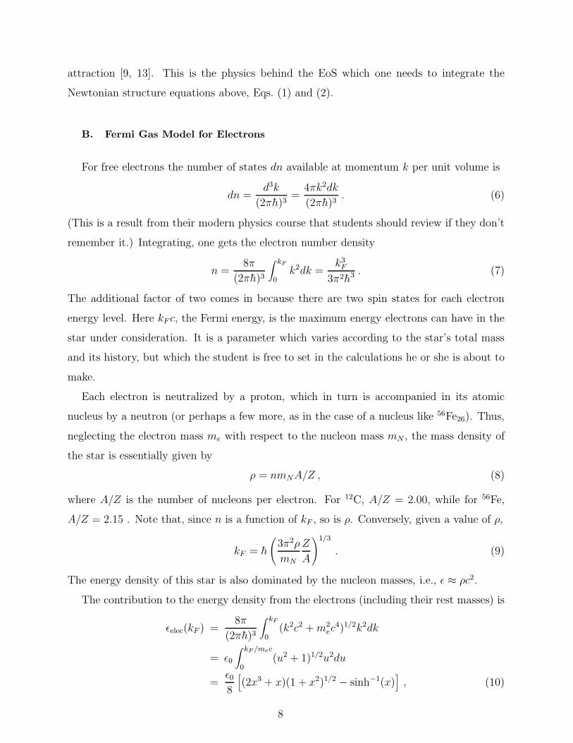
B. Fermi Gas Model for Electrons

For free electrons the number of states dn available at momentum k per unit volume is

dn =d3k

(2πh)3=

4πk2dk

(2πh)3. (6)

(This is a result from their modern physics course that students should review if they don’t

remember it.) Integrating, one gets the electron number density

n =8π

(2πh)3

∫ kF

0k2dk =

k3F

3π2h3 . (7)

The additional factor of two comes in because there are two spin states for each electron

energy level. Here kF c, the Fermi energy, is the maximum energy electrons can have in the

star under consideration. It is a parameter which varies according to the star’s total mass

and its history, but which the student is free to set in the calculations he or she is about to

make.

Each electron is neutralized by a proton, which in turn is accompanied in its atomic

nucleus by a neutron (or perhaps a few more, as in the case of a nucleus like 56Fe26). Thus,

neglecting the electron mass me with respect to the nucleon mass mN , the mass density of

the star is essentially given by

ρ = nmNA/Z , (8)

where A/Z is the number of nucleons per electron. For 12C, A/Z = 2.00, while for 56Fe,

A/Z = 2.15 . Note that, since n is a function of kF , so is ρ. Conversely, given a value of ρ,

kF = h

(

3π2ρ

mN

Z

A

)1/3

. (9)

The energy density of this star is also dominated by the nucleon masses, i.e., ǫ ≈ ρc2.

The contribution to the energy density from the electrons (including their rest masses) is

ǫelec(kF ) =8π

(2πh)3

∫ kF

0(k2c2 + m2

ec4)1/2k2dk

= ǫ0

∫ kF /mec

0(u2 + 1)1/2u2du

=ǫ0

8

[

(2x3 + x)(1 + x2)1/2 − sinh−1(x)]

, (10)

8

where

ǫ0 =m4

ec5

π2h3 (11)

carries the desired dimensions of energy per volume and x = kF /mec. The total energy

density is then

ǫ = nmNA/Z + ǫelec(kF ) . (12)

One should check that the first term here is much larger than the second.

To get our desired EoS, we need an expression for the pressure. The following presents a

problem (!) that the student should work through. From the first law of thermodynamics,

dU = dQ − pdV , then at temperature T fixed at T = 0 (where dQ = 0 since dT = 0)

p = − ∂U

∂V

]

T=0

= n2 d(ǫ/n)

dn= n

dǫ

dn− ǫ = nµ − ǫ , (13)

where the energy density here is the total one given by Eq. (12). The quantity µi = dǫ/dni

defined in the last equality is known as the chemical potential of the electrons. This is a

concept which will be especially useful in Section 5 where we consider an equilibrium mix

of neutrons, protons and electrons.

Utilizing Eq. (10), Eq. (13) yields the pressure (another problem!)

p(kF ) =8π

3(2πh)3

∫ kF

0(k2c2 + m2

ec4)−1/2k4dk

=ǫ0

3

∫ kF /mec

0(u2 + 1)−1/2u4du

=ǫ0

24

[

(2x3 − 3x)(1 + x2)1/2 + 3 sinh−1(x)]

. (14)

(Hint: use the n2d(ǫ/n)/dn form and remember to integrate by parts.)

Using Mathematica [14] the student can show that the constant ǫ0 = 1.42× 1024 in units

that, at this point, are erg/cm3. (Yet another problem: verify that the units of ǫ0 are as

claimed [15].) One also finds that Mathematica can perform the integrals analytically. (We

quoted the results already in the equations above.) They are a bit messy, however, as they

both involve an inverse hyperbolic sine function, and thus are not terribly enlightening. It

is useful, however, for the student to make a plot of ǫ versus p (such as shown in Fig. 2) for

values of the parameter 0 ≤ kF ≤ 2me. This curve has a shape much like ǫ4/3 (the student

should compare with this), and there is a good reason for that.

9

p(ǫ)

5.·1027 1.·1028

5.·1023

1.·1024

1.5·1024

FIG. 2: Relation between pressure p (y-axis) and energy density ǫ (x-axis) in the free electron

Fermi gas model. Units are ergs/cm3. Note that the pressure is much smaller than the energy

density, since the latter is dominated by the massive nucleons.

Consider the (relativistic) case when kF ≫ me. Then Eq. (14) simplifies to

p(kF ) =ǫ0

3

∫ kF /mec

0u3du =

ǫ0

12(kF/mec)

4 =hc

12π2

(

3π2Zρ

mNA

)4/3

≈ Krel ǫ4/3 , (15)

where

Krel =hc

12π2

(

3π2Z

AmNc2

)4/3

. (16)

A star having simple EoS like p = Kǫγ is called a “polytrope”, and we therefore see that the

relativistic electron Fermi gas gives a polytropic EoS with γ = 4/3. As will be seen in the

next subsection, a polytropic EoS allows one to solve the structure equations (numerically)

in a relatively straight-forward way [16].

There is another polytropic EoS for the non-interacting electron Fermi gas model corre-

sponding to the non-relativistic limit, where kF ≪ me. In a way similar to the derivation of

Eq. (15), one finds

p = Knon−relǫ5/3 , where Knon−rel =

h2

15π2me

(

3π2Z

AmNc2

)5/3

. (17)

[Question: what are the units of Krel and Knon−rel? Task: confirm that in the appropriate

limits, Eqs. (10) and (14) reduce to those in Eqs. (15) and (17).]

10

C. The Structure Equations for a Polytrope

As mentioned earlier, we want to express our results in units of km and M⊙. Thus it is

useful to define M(r) = M(r)/M⊙. The first Newtonian structure equation, Eq. (1), then

becomesdp(r)

dr= −R0

ǫ(r)M(r)

r2, (18)

where the constant R0 = GM⊙/c2 = 1.47 km. (That is, for those who already know, R0 is

one half the Schwartzschild radius of our sun.) In this equation p and ǫ still carry dimensions

of, say, ergs/cm3. Therefore, let us define dimensionless energy density and pressure, ǫ and

p, by

p = ǫ0p , ǫ = ǫ0ǫ (19)

where ǫ0 has dimensions of energy density. This ǫ0 is not the same as defined in Eq. (11).

Its numerical choice here is arbitrary, and a suitable strategy is to make that choice based

on the dimensionful numbers that define the problem at hand. We’ll employ this strategy

to fix it below. For a polytrope, we can write

p = Kǫ γ , where K = Kǫ γ−10 is dimensionless. (20)

It is easier to solve Eq. (18) for p, so we should express ǫ in terms of it,

ǫ = (p/K)1/γ . (21)

Equation (18) can now be recast in the form

dp(r)

dr= −α p(r)1/γM(r)

r2, (22)

where the constant α is

α = R0/K1/γ = R0/(Kǫγ−1

0 )1/γ . (23)

Equation (22) has dimensions of 1/km, with α in km (since R0 is). That is, it is to be

integrated with respect to r, with r also in km.

We can choose any convenient value for α since ǫ0 is still free. For a given value of α, ǫ0

is then fixed at

ǫ0 =

[

1

K

(

R0

α

)γ]1−γ

. (24)

11

We also need to cast the other coupled equation, Eq. (2), in terms of dimensionless p and

M,dM(r)

dr= βr2p(r)1/γ , (25)

where [17]

β =4πǫ0

M⊙c2K1/γ=

4πǫ0

M⊙c2(Kǫγ−10 )1/γ

. (26)

Equation (25) also carries dimensions of 1/km, the constant β having dimesnions 1/km3.

Note that, in integrating out from r = 0, the initial value of M(0) = 0.

D. Integrating the Polytrope Numerically

Our task is to integrate the coupled first-order differential equations (DE), Eqs. (22) and

(25), out from the origin, r = 0, to the point R where the pressure falls to zero, p(R) = 0

[18]. To do this we need two initial values, p(0) (which must be positive) and M(0) ( which

we already know must be 0). The star’s radius, R, and its mass M = M(R) in units of M⊙

will vary, depending on the choice for p(0).

For purposes of numerical stability in solving Eqs. (22) and (25), we want the constants

α and β to be not much different from each other (and probably not much different from 1).

We will see below that this can be arranged for both of the two polytropic EoS’s discussed

above for white dwarfs.

Our coupled DE’s are quite non-linear. In fact, because of the p1/γ factors, the solution

will become complex when p(r) < 0, i.e., when r > R. Thus we will want to recognize when

this happens. How can this be programmed?

Mathematica and similar symbolic/numerical packages have built-in first-order DE

solvers. Perhaps the solver is as simple as a fixed, equal-step Runge-Kutta routine (as

in MathCad 7 Standard), but there are often more sophisticated solvers in more recent ver-

sions. These packages also allow for program control constructs such as do-loops, whiles and

the like.

Thus, consider a do-loop on a variable r running in appropriately small steps over a

range that is sure to contain the expected value of R. Call the DE solver inside this loop,

integrating the coupled DE’s from r = 0 to r. When the solver routine exits, check to see if

the last value of p, i.e., p(r), has a real part which has gone negative. If so, then break out

12

of the loop, calling R = r. If not, go on to the next larger value of r and call the DE solver

again.

More discussion of how to program the integration of the DE’s is inappropriate here,

since we want to encourage the student to learn from programming to appreciate how the

symbolic/numerical package is used.

E. The Relativistic Case kF ≫ me

This is the regime for white dwarfs with the largest mass. A larger mass needs a greater

central pressure to support it. However, large central pressures mean the squeezed electrons

become relativistic.

Recall that the polytrope exponent γ = 4/3 for this case and the equation of state is

given by P = Krelǫγ with Krel given by Eq. (16). After some trial and error, we chose in our

program (the student may want to try something else)

α = R0 = 1.473 km [kF ≫ me] , (27)

which in turn fixes, from Eq. (24),

ǫ0 = 7.463 × 1039ergs/cm3 = 4.17 M⊙c2/km3 [kF ≫ me] . (28)

The first question the student should ask, in checking this number, is whether such a large

number is physically reasonable.

Continuing with the kF ≫ me numerics, Eqs. (16) and (26) give

β = 52.46 /km3 [kF ≫ me] , (29)

which is about 30 times larger than α, but probably manageable from the standpoint of

performing the numerical integration.

In our first attempt to integrate the coupled DE’s for this case (using a do-loop as

described above) we chose p(0) = 1.0. This gives us a white dwarf of radius R ≈ 2 km,

which is miniscule compared with the expected radius of ≈ 104 km! Why? What went

wrong?

The student who also makes this kind of mistake will eventually realize that our choice

of scale, ǫ0 = 4.17M⊙c2/km3, represents a huge energy density. One can simply estimate the

13

TABLE I: Radius R (in km) and mass M (in M⊙) for white dwarfs with a relativistic electron

Fermi gas EoS.

p(0) R M

10−14 4840 1.2431

10−15 8600 1.2432

10−16 15080 1.2430

average energy density of a star with a 104 km radius and a mass of one solar mass by the

ratio of its rest mass energy to its volume,

〈ǫ〉 ≈ M⊙c2

R3= 10−12 M⊙c2/km3 , (30)

which is much, much smaller than the ǫ0 here. In addition, the pressure p is about 2000

times smaller than the energy density ǫ (see Fig. 2). Thus, choosing a starting value of

p(0) ∼ 10−15 would probably be more physical.

Doing so does give much more reasonable results. Table I shows our program’s results

for R and M and how they depend on p(0). The surprise here is that, within the numerical

error expected, all these cases have the same mass! Increasing the central pressure doesn’t

allow the star to be more massive, just more compact.

It turns out that this result is correct, i.e., that the white dwarf mass is independent of

the choice of the central pressure. It is not easy to see this, however, from the numerical

integration we have done here. The discussion in terms of Lane-Emden functions [16] shows

why, though the mathematics here might be a bit steep for many undergraduates. For this

reason, we quote without proof the analytic results. For the case of a polytropic equation

of state p = Kǫγ , the mass

M = 4πǫ2(γ− 4

3)/3

(

Kγ

4πG(γ − 1)

)3/2

ζ21 |θ(ζ1)| , (31)

and the radius

R =

√

Kγ

4πG(γ − 1)ζ1 ǫ(γ−2)/2 . (32)

In the above-mentioned solutions, ζ1 and θ(ζ1) are numerical constants that depend on the

polytropic index γ. By examining Eq. (31), we see that for γ = 4/3 the mass is independent

of the central energy density, and hence also the central pressure p0. Also, note that from

14

5000 10000 15000

5.·10-17

1.·10-16

5000 10000 15000

0.5

1

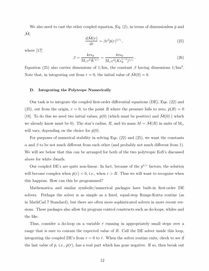
FIG. 3: p(r) and M(r) for white dwarfs using the relativistic electron Fermi gas model. Here

p(0) = 10−16.

Eq. (32), the radius decreases with increasing central pressure as R ∝ p(γ−2)/2γ0 = p

−1/40 .

In any case, the student should notice this point and use it as check of the numerical

results obtained. Figure 3 shows the dependence of p(r) and M(r) on distance for the case

p(0) = 10−16. It is interesting that p(r) becomes small and essentially flat around 8000 km

before finally going through zero at R = 15, 080 km.

The results and graphs shown here were generated with a Mathematica 4.0 program, but

we were able to reproduce them using MathCad 7 Standard. In that case, however, program-

ming a loop is difficult, so we searched by hand for the endpoint (where the real part of p(r)

goes negative). More recent versions of MathCad have more complete program constructs,

such as while-loops, so this process could undoubtedly be automated. (Alternatively, the

student might try to solve for a root of p(r) = 0.)

15

F. The Non-Relativistic Case, kF ≪ me

Eventually, as the central pressure p(0) gets smaller, the electron gas is no longer rela-

tivistic. Also as the pressure gets smaller, it can support less mass. This moves us in the

direction of the less massive white dwarfs, and, as it turns out, these dwarfs are larger (in

radius) than the ones in the last section.

In the extreme case, when kF ≪ me, we can integrate the structure equations for the

other polytropic EoS, where γ = 5/3. The programming for this is very much the same as

in the 4/3 case, but the numbers involved are quite different (as are the results).

Inserting the values of the physical constants in Eq. (17), we find

Knon−rel = 3.309 × 10−23 cm2

ergs2/3. (33)

This time, however, and after some experimentation, we chose the constant

α = 0.05 km [kF ≪ me] , (34)

which then fixes

ǫ0 = 2.488 × 1037ergs/cm3 = 0.01392 M⊙c2/km3 [kF ≪ me] . (35)

Note that this ǫ0 is much smaller than our choice for the relativistic case. The other constant

we need, from Eq. (26), is

β = 0.005924 /km3 [kF ≪ me] , (36)

which, unlike the relativistic case, is not larger than α but smaller.

When we first ran our Mathematica code for this case, we (inadvertantly) tried a value

of p(0) = 10−12. This gave us a star with radius R = 5310 km and mass M = 3.131. Oops!,

that mass is bigger than the largest mass of 1.243 that we found for the relativistic EoS!

What did we do wrong?

What happened (and the student can set up her program so this trap can be avoided)

is that the choice p(0) = 10−12 violates the assumption that kF ≪ me. One really needs

values for p(0) < 4 × 10−15. This says, in fact, that the relativistic p(0) = 10−16 case that

we plotted in Fig. 3 is not really relativistic.

Results for the non-relativistic case for the last two values of p(0) in Table I are shown in

Table II. It is quite instructive to compare the differences in the two tables. The masses are,

16

TABLE II: Radius R (in km) and mass M (in M⊙) for white dwarfs with a non-relativistic electron

Fermi gas EoS.

p(0) R M

10−15 10620 0.3941

10−16 13360 0.1974

p(r)

5000 10000

5.·10-17

1.·10-16

FIG. 4: p(r) for a white dwarf using the non-relativistic electron Fermi gas model with central

pressure p(0) = 10−16.

of course, smaller, as expected, and now they vary with p(0). Somewhat surprising is that

the non-relativistic radius is bigger for p(0) = 10−15 but smaller for p(0) = 10−16. Figure 4

shows the pressure distribution for the latter case, to be compared with the corresponding

graph in Fig. 3. Note that this pressure curve does not have the peculiar, long flat tail

found using the relativistic EoS.

In fact, by this time the student should have realized that neither of these polytropes is

very physical, at least not for all cases. The non-relativistic assumption certainly does not

work for central pressures p(0) > 10−14, i.e., for the more massive (and more common) white

dwarfs. On the other hand, the relativistic EoS certainly should not work when the pressure

becomes small, i.e., in the outer regions of the star (where it eventually goes to zero at the

star’s radius). So, can one find an EoS to cover the whole range of pressures?

We haven’t actually done this for white dwarfs, but the program would be much like that

discussed below for the full neutron star. Given the transcendental expressions for energy

17

and pressure that generate the curve shown in Fig. 2, it should be possible to find a fit

(using, for example, the built-in fitting function of Mathematica) like

ǫ(p) = ANRp3/5 + ARp3/4 . (37)

The second term dominates at high pressures (the relativistic case), but the first term takes

over for low pressures when the kF ≫ me assumption does not hold. (Setting the two terms

equal and solving for p, as Chandrasekhar and Fowler did, gives the value of p when special

relativity starts to be important.) This expression for ǫ(p) could then be used in place of the

p1/γ factors on the right hand sides of the structure equations. Proceed to solve numerically

as before. We leave this as an exercise for the interested student.

IV. PURE NEUTRON STAR, FERMI GAS EOS

Having by now become warm, the student can now tackle neutron stars. Here one must

include the general relativistic (GR) contributions represented by the three dimensionless

factors in the TOV equation, Eq. (5). One of the first things that comes to mind is how one

deals numerically with the (apparent) singularities in these factors at r = 0 [19].

Also, as in the case of the white dwarfs, there is a question of what to use for the EoS.

In this section we show what can be done for pure neutron stars, once again using a Fermi

gas model for, now, a neutron gas instead of an electron gas. Such a model, however, is

unrealistic for two reasons. First, a real neutron star consists not just of neutrons but

contains a small fraction of protons and electrons (to inhibit the neutrons from decaying

into protons and electrons by their weak interactions). Second, the Fermi gas model ignores

the strong nucleon-nucleon interactions, which give important contributions to the energy

density. Each of these points will be dealt with in sections below.

A. The Non-Relativistic Case, kF ≪ mn

For a pure neutron star Fermi gas EoS one can proceed much as in the white dwarf case,

substituting the neutron mass mn for the electron mass me in the equations found in Sec.

3. When kF ≪ mn one finds, again, a polytrope with γ = 5/3. (More exercises for the

18

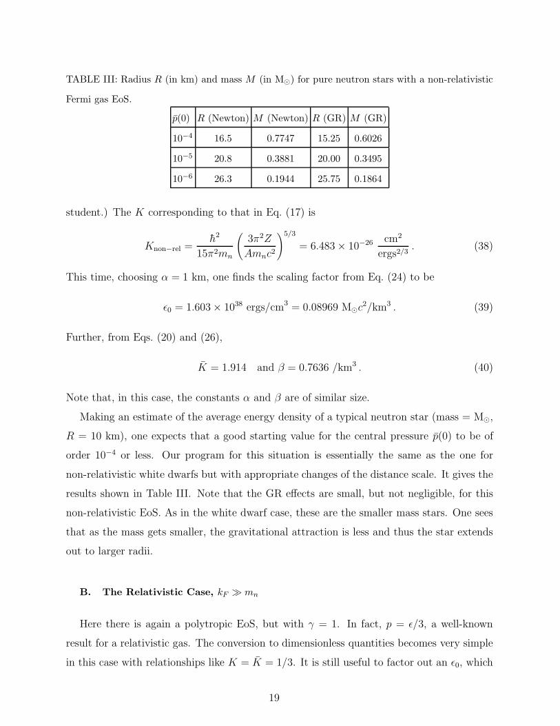
TABLE III: Radius R (in km) and mass M (in M⊙) for pure neutron stars with a non-relativistic

Fermi gas EoS.

p(0) R (Newton) M (Newton) R (GR) M (GR)

10−4 16.5 0.7747 15.25 0.6026

10−5 20.8 0.3881 20.00 0.3495

10−6 26.3 0.1944 25.75 0.1864

student.) The K corresponding to that in Eq. (17) is

Knon−rel =h2

15π2mn

(

3π2Z

Amnc2

)5/3

= 6.483 × 10−26 cm2

ergs2/3. (38)

This time, choosing α = 1 km, one finds the scaling factor from Eq. (24) to be

ǫ0 = 1.603 × 1038 ergs/cm3 = 0.08969 M⊙c2/km3 . (39)

Further, from Eqs. (20) and (26),

K = 1.914 and β = 0.7636 /km3 . (40)

Note that, in this case, the constants α and β are of similar size.

Making an estimate of the average energy density of a typical neutron star (mass = M⊙,

R = 10 km), one expects that a good starting value for the central pressure p(0) to be of

order 10−4 or less. Our program for this situation is essentially the same as the one for

non-relativistic white dwarfs but with appropriate changes of the distance scale. It gives the

results shown in Table III. Note that the GR effects are small, but not negligible, for this

non-relativistic EoS. As in the white dwarf case, these are the smaller mass stars. One sees

that as the mass gets smaller, the gravitational attraction is less and thus the star extends

out to larger radii.

B. The Relativistic Case, kF ≫ mn

Here there is again a polytropic EoS, but with γ = 1. In fact, p = ǫ/3, a well-known

result for a relativistic gas. The conversion to dimensionless quantities becomes very simple

in this case with relationships like K = K = 1/3. It is still useful to factor out an ǫ0, which

19

in our program we took to have a value 1.6× 1038 erg/cm3, as suggested by the value in the

previous sub-section. Then, if we choose this time

α = 3R0 = 4.428 km (41)

we find

β = 3.374 /km3 . (42)

We expect central pressures p(0) in this case to be greater than 10−4. Other than these

changes, we wrote a similar program to the one above, taking care to avoid exponents like

1/(γ − 1).

Running that code gives, at first glance, enormous radii, values of R greater than 50

km! We can imagine the student looking frantically for a program bug that isn’t there. In

fact, what really happens is that, for this EoS, the loop on r runs through its whole range,

since the pressure p(r) never passes through zero. (A plot of p(r) looks quite similar, but

for distance scale, to that shown in Fig. 3, where γ = 4/5.) It only falls monotonically

toward zero, getting ever smaller. By the time the student recognizes this, she will probably

also have realized that the relativistic gas EoS is inappropriate for such small pressures.

Something better should be done (as in the next sub-section).

It turns out that the structure equations for γ = 1 are sufficiently simple that an analytic

solution for p(r) can be found, which corroborates the above remarks about not having a

zero at a finite R. A suggestion for the student is to try a power-law Ansatz.

C. The Fermi Gas EoS for Arbitrary Relativity

In order to avoid the trap of the relativistic gas, one should find an EoS for the non-

interacting neutron Fermi gas which works for all values of the relativity parameter x =

kF/mnc. Taking a hint from the two polytropes, one can try to fit the energy density as a

function of pressure, each given as a transcendental function of kF , with the form

ǫ(p) = ANRp3/5 + ARp . (43)

For low pressures the non-relativistic first term dominates over the second. (The power in

the relativistic term is changed from that in Eq. (37).) It is again useful to factor out an ǫ0

20

from both ǫ and p. In this case, it is more natural to define it as

ǫ0 =m4

nc5

(3π2h)3= 5.346 × 1036 ergs

cm3= 0.003006

M⊙c2

km3 . (44)

Mathematica can easily create a table of exact ǫ and p values as a function of kF . The

dimensionless A-values can then be fit using its built-in fitting function. From our efforts

we found, to an accuracy of better than 1% over most of the range of kF [20],

ANR = 2.4216 , AR = 2.8663 . (45)

We used the fitted functional form for ǫ of Eq. (43) in a Mathematica program similar

to that for the neutron star based on the non-relativistic EoS. With the ǫ0 of Eq. (44) and

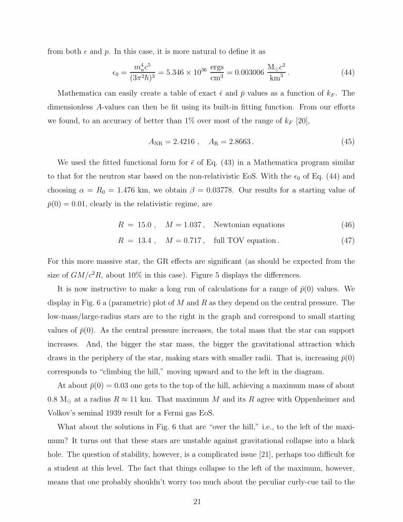
choosing α = R0 = 1.476 km, we obtain β = 0.03778. Our results for a starting value of

p(0) = 0.01, clearly in the relativistic regime, are

R = 15.0 , M = 1.037 , Newtonian equations (46)

R = 13.4 , M = 0.717 , full TOV equation . (47)

For this more massive star, the GR effects are significant (as should be expected from the

size of GM/c2R, about 10% in this case). Figure 5 displays the differences.

It is now instructive to make a long run of calculations for a range of p(0) values. We

display in Fig. 6 a (parametric) plot of M and R as they depend on the central pressure. The

low-mass/large-radius stars are to the right in the graph and correspond to small starting

values of p(0). As the central pressure increases, the total mass that the star can support

increases. And, the bigger the star mass, the bigger the gravitational attraction which

draws in the periphery of the star, making stars with smaller radii. That is, increasing p(0)

corresponds to “climbing the hill,” moving upward and to the left in the diagram.

At about p(0) = 0.03 one gets to the top of the hill, achieving a maximum mass of about

0.8 M⊙ at a radius R ≈ 11 km. That maximum M and its R agree with Oppenheimer and

Volkov’s seminal 1939 result for a Fermi gas EoS.

What about the solutions in Fig. 6 that are “over the hill,” i.e., to the left of the maxi-

mum? It turns out that these stars are unstable against gravitational collapse into a black

hole. The question of stability, however, is a complicated issue [21], perhaps too difficult for

a student at this level. The fact that things collapse to the left of the maximum, however,

means that one probably shouldn’t worry too much about the peculiar curly-cue tail to the

21

2 4 6 8 10 12r

0.002

0.004

0.006

0.008

0.01

2 4 6 8 10 12r

0.2

0.4

0.6

0.8

1

FIG. 5: p(r) and M(r) (r in km) for a pure neutron star with central pressure p(0) = 0.01, using a

Fermi gas EoS fit valid for all values of kF . The thin curves are results from the classical Newtonian

structure equations, while the thick ones include general relativistic corrections.

M-R curve in the figure. It appears to be an artifact for very large values of p(0), also seen

in other calculations, even though it is especially prominent for this Fermi gas EoS.

D. Why Is There a Maximum Mass?

On general grounds one can argue that cold compact objects such as white dwarfs and

neutron stars must possess a limiting mass beyond which stable hydrostatic configurations

are not possible. This limiting mass is often called the maximum mass of the object and

was briefly mentioned in the discussion at the end of Sec. 2.2 and that relating to Fig. 6. In

what follows, we outline the general argument.

22

M(R)

5 10 15 20 25

0.2

0.4

0.6

0.8

1

FIG. 6: The mass M (in M⊙) and radius R (in km) for pure neutron stars, using a Fermi gas

EoS. The stars of low mass and large radius are solutions of the TOV equations for small values

of central pressure p(0). The stars to the right of the maximum at R = 11 are stable, while those

to the left will suffer gravitational collapse.

The thermal component of the pressure in cold stars is by definition negligible. Thus,

variations in both the energy density and pressure are only caused by changes in the density.

Given this simple observation, let us examine why we expect a maximum mass in the

Newtonian case.

Here, an increase in the density results in a proportional increase in the energy density.

This results in a corresponding increase in the gravitational attraction. To balance this,

we require that the increment in pressure is large enough. However, the rate of change

of pressure with respect to energy density is related to the speed of sound (see Sec. 6.3).

In a purely Newtonian world, this is in principle unbounded. However, the speed of all

propagating signals cannot exceed the speed of light. This then puts a bound on the pressure

increment associated with changes in density.

Once we accept this bound, we can safely conclude that all cold compact objects will

eventually run into the situation in which any increase in density will result in an additional

gravitational attraction that cannot be compensated for by the corresponding increment in

pressure. This leads naturally to the existence of a limiting mass for the star.

When we include general relativistic corrections, as discussed in Sec. 2.2 earlier, they act

to “amplify” gravity. Thus we can expect the maximum mass to occur at a somewhat lower

23

mass than in the Newtonian case.

V. NEUTRON STARS WITH PROTONS AND ELECTRONS, FERMI GAS EOS

As mentioned at the beginning of the last section, neutron stars are not made only of

neutrons. There must also be a small fraction of protons and electrons present. The reason

for this is that a free neutron will undergo a weak decay,

n → p + e− + νe , (48)

with a lifetime of about 15 minutes. So, there must be something that prevents this decay

in the case of the star, and that is the presence of the protons and electrons.

The decay products have low energies (mn − mp − me = 0.778 MeV), with most of that

energy being carried away by the light electron and (nearly massless) neutrino [22]. If all

the available low-energy levels for the decay proton are already filled by the protons already

present, then the Pauli exclusion principle takes over and prevents the decay from taking

place.

The same might be said about the presence of the electrons, but in any case the electrons

must be present within the star to cancel the positive charge of the protons. A neutron star

is electrically neutral. We saw earlier that the number density of a particle species is fixed

in terms of that particle’s Fermi momentum [see Eq. (7)]. Thus equal numbers of electrons

and protons implies that

kF,p = kF,e . (49)

In addition to charge neutrality, we also require weak interaction equilibrium, i.e., as

many neutron decays [Eq. (48)] taking place as electron capture reactions, p + e− → n + νe.

This equilibrium can be expressed in terms of the chemical potentials for the three particle

species,

µn = µp + µe . (50)

We already defined the chemical equilibrium for a particle in Sec. 3.2 after Eq. (13),

µi(kF,i) =dǫ

dn= (k2

F,i + m2i )

1/2 , i = n, p, e . (51)

where, for the time being, we have set c = 1 to simplify the equations somewhat. (The

student is urged to prove the right-hand equality.) From Eqs. (49), (50), and (51) we can

24

find a constraint determining kF,p for a given kF,n,

(k2F,n + m2

n)1/2 − (k2F,p + m2

p)1/2 − (k2

F,p + m2e)

1/2 = 0 . (52)

While an ambitious algebraist can probably solve this equation for kF,p as a function of kF,n,

we were somewhat lazy and let Mathematica do it, finding

kF,p(kF,n) =[(k2

F,n + m2n − m2

e)2 − 2m2

p(k2F,n + m2

n + m2e) + m4

p]1/2

2(k2F,n + m2

n)1/2(53)

≈ k2F,n + m2

n − m2p

2(k2F,n + m2

n)1/2for

me

kF,n→ 0 . (54)

The total energy density is the sum of the individual energy densities,

ǫtot =∑

i=n,p,e

ǫi , (55)

where

ǫi(kF,i) =∫ kF,i

0(k2 + mi)

1/2k2dk = ǫ0 ǫi(xi, yi) , (56)

and, as before [23],

ǫ0 = m4n/3π2h3 , (57)

ǫi(xi, yi) =∫ xi

0(u2 + y2

i )1/2u2du , (58)

xi = kF,i/mi , yi = mi/mn . (59)

The corresponding total pressure is

ptot =∑

i=n,p,e

pi , (60)

pi(kF,i) =∫ kF,i

0(k2 + mi)

−1/2k4dk = ǫ0 pi(xi, yi) , (61)

pi(xi, yi) =∫ xi

0(u2 + y2

i )−1/2u4du . (62)

Using Mathematica the (dimensionless) integrals can be expressed in terms of log and

sinh−1 functions of xi and yi. One can then generate a table of ǫtot versus ptot values for an

appropriate range of kF,n’s. This, in turn, can be fitted to the same form of two terms as

before in Eq. (43). We found, this time, the coefficients to be

ANR = 2.572 , AR = 2.891 . (63)

These coefficients are not much changed from those in Eq. (45) for the pure neutron star.

Therefore, we expect that the M versus R diagram for this more realistic Fermi gas model

would not be much different from that in Fig. 6.

25

VI. INTRODUCING NUCLEAR INTERACTIONS

Nucleon-nucleon interactions can be included in the EoS (they are important) by con-

structing a simple model for the nuclear potential that reproduces the general features of

(normal) nuclear matter. In doing so we were much guided by the lectures of Prakash [6].

We will use MeV and fm (10−13 cm) as our energy and distance units for much of this

section, converting back to M⊙ and km later. We will also continue setting c = 1 for now.

In this regard, the important number to remember for making conversions is hc = 197.3

MeV-fm. We will also neglect the mass difference between protons and neutrons, labeling

their masses as mN .

The von Weizacker mass formula [24] for nuclides with Z protons and N neutrons gives,

for normal symmetric nuclear matter (A = N + Z with N = Z), an equilibrium number

density n0 of 0.16 nucleons/fm3. For this value of n0 the Fermi momentum is k0F = 263

MeV/c [see Eq. (7)]. This momentum is small enough compared with mN = 939 MeV/c2

to allow a non-relativistic treatment of normal nuclear matter. At this density, the average

binding energy per nucleon, BE = E/A−mN , is −16 MeV. These are two physical quantities

we definitely want our nuclear potential to respect, but there are two more that we’ll need

to fix the parameters of the model.

We chose one of these as the nuclear compressibility, K0, to be defined below. This is a

quantity which is not all that well established but is in the range of 200 to 400 MeV. The

other is the so-called symmetry energy term, which, when Z = 0, contributes about 30 MeV

of energy above the symmetric matter minimum at n0. (This quantity might really be better

described as an asymmetry parameter, since it accounts for the energy that comes in when

N 6= Z.)

A. Symmetric Nuclear Matter

We defer the case when N 6= Z, which is our main interest in this paper, to the next

sub-section. Here we concentrate on getting a good (enough) EoS for nuclear matter when

N = Z, or, equivalently, when the proton and neutron number densities are equal, nn = np.

The total nucleon density n = nn + np.

We need to relate the first three nuclear quantities, n0, BE, and K0 to the energy density

26

for symmetric nuclear matter, ǫ(n). Here n = n(kF ) is the nuclear density (at and away

from n0). We will not worry in this section about the electrons that are present, since, as

was seen in the last section, its contribution is small. The energy density now will include

the nuclear potential, V (n), which we will model below in terms of two simple functions

with three parameters that are fitted to reproduce the above three nuclear quantities. [The

fourth quantity, the symmetry energy, will be used in the next sub-section to fix a term in

the potential which is proportional to (N − Z)/A.]

First, the average energy per nucleon, E/A, for symmetric nuclear matter is related to ǫ

by

E(n)/A = ǫ(n)/n , (64)

which includes the rest mass energy, mN and has dimensions of MeV. As a function of n,

E(n)/A − mN has a minimum at n = n0 with a depth BE = −16 MeV. This minimum

occurs whend

dn

(

E(n)

A

)

=d

dn

(

ǫ(n)

n

)

= 0 at n = n0 . (65)

This is one constraint of the parameters of V (n). Another, of course, is the binding energy,

ǫ(n)

n− mN = BE at n = n0 . (66)

The positive curvature at the bottom of this valley is related to the nuclear (in)compress-

ibility by [25]

K(n) = 9dp(n)

dn= 9

[

n2 d2

dn2

(

ǫ

n

)

+ 2nd

dn

(

ǫ

n

)

]

, (67)

using Eq. (13), which defines the pressure in terms of the energy density. At n = n0 this

quantity equals K0. (The factor of 9 is a historical artifact from the convention originally

defining K0.)

(Question: why does one not have to calculate the pressure at n = n0?)

The N = Z potential in ǫ(n) we will model as [6]

ǫ(n)

n= mN +

3

5

h2k2F

2mN+

A

2u +

B

σ + 1uσ , (68)

where u = n/n0 and σ are dimensionless and A and B have dimensions of MeV. The first

term represents the rest mass energy and the second the average kinetic energy per nucleon.

[These two terms are leading in the non-relativistic limit of the nucleonic version of Eq.

27

(10).] For kF (n0) = k0F we will abbreviate the kinetic energy term as 〈E0

F 〉, which evaluates

to 22.1 MeV. The kinetic energy term in Eq. (68) can be better written as 〈E0F 〉 u2/3.

From the above three constraints, Eqs. (65)-(67), and noting that u = 1 at n = n0, we

get three equations for the parameters A, B, and σ:

⟨

E0F

⟩

+A

2+

B

σ + 1= BE , (69)

2

3

⟨

E0F

⟩

+A

2+

Bσ

σ + 1= 0 , (70)

10

9

⟨

E0F

⟩

+ A + Bσ =K0

9. (71)

Solving these equations (which we found easier to do by hand than with Mathematica), one

finds

σ =K0 + 2 〈E0

F 〉3 〈E0

F 〉 − 9BE, (72)

B =σ + 1

σ − 1

[

1

3

⟨

E0F

⟩

− BE]

, (73)

A = BE − 5

3

⟨

E0F

⟩

− B . (74)

Numerically, for K0 = 400 MeV (which is perhaps a high value),

A = −122.2 MeV, B = 65.39 MeV, σ = 2.112 . (75)

Note that σ > 1, a point we will come back to below, since it violates a basic principle of

physics called “causality.”

The student can try other values of K0 to see how the parameters A, B, and σ change.

More interesting is to see how the interplay between the A- and B-terms gives the valley at

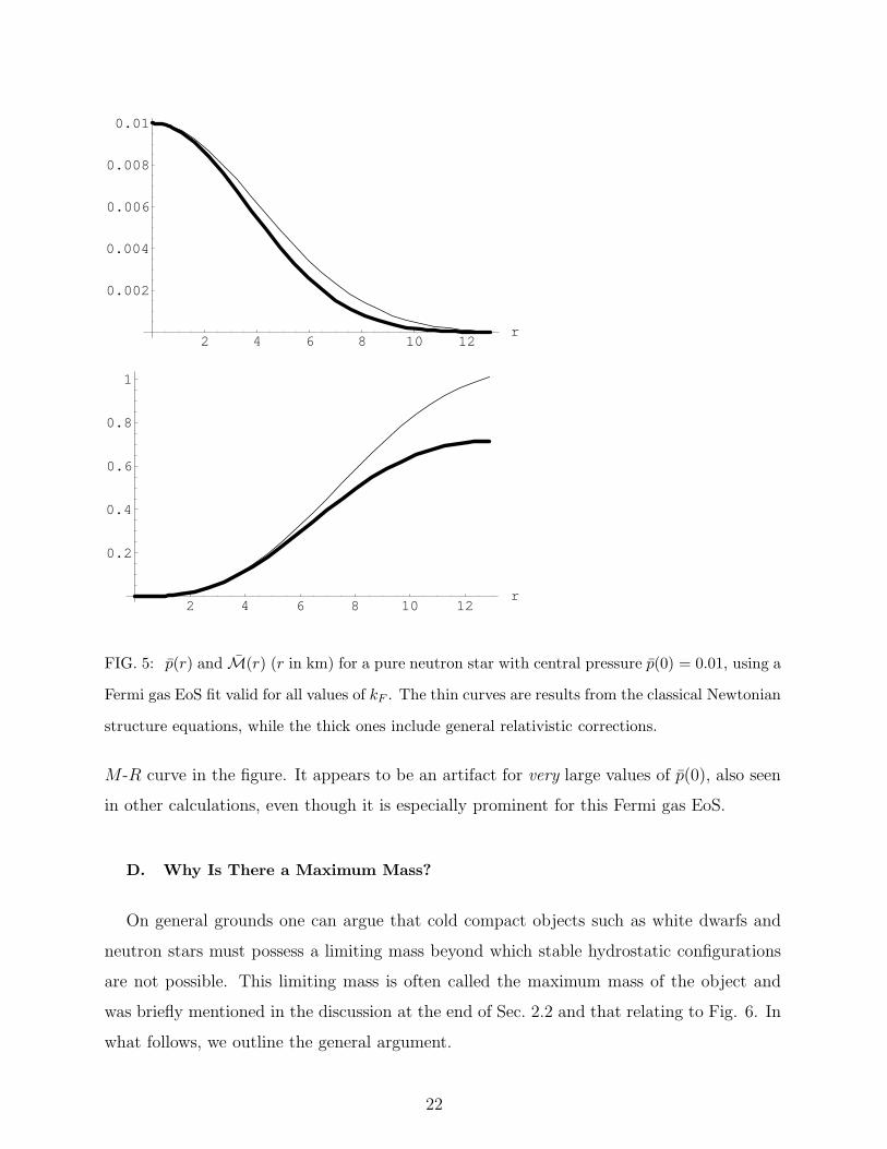
n = n0. Figure 7 shows E/A−mN as a function of n using the parameters of Eq. (75). We

would hope the student notices the funny little positive bump in this plot near n = 0 and

sorts out the reason for its occurrence.

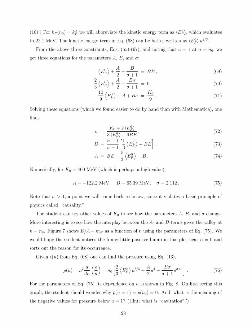
Given ǫ(n) from Eq. (68) one can find the pressure using Eq. (13),

p(n) = n2 d

dn

(

ǫ

n

)

= n0

[

2

3

⟨

E0F

⟩

u5/3 +A

2u2 +

Bσ

σ + 1uσ+1

]

. (76)

For the parameters of Eq. (75) its dependence on n is shown in Fig. 8. On first seeing this

graph, the student should wonder why p(u = 1) = p(n0) = 0. And, what is the meaning of

the negative values for pressure below u = 1? (Hint: what is “cavitation”?)

28

E/A − mN

0.5 1 1.5 2u

-15

-10

-5

5

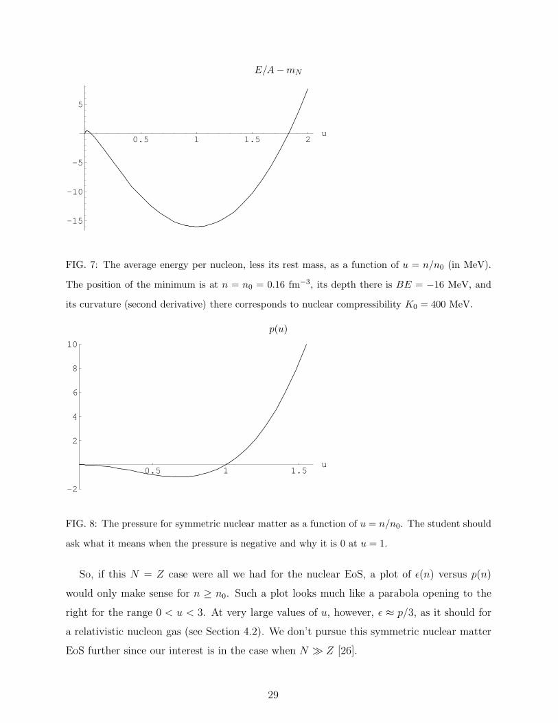
FIG. 7: The average energy per nucleon, less its rest mass, as a function of u = n/n0 (in MeV).

The position of the minimum is at n = n0 = 0.16 fm−3, its depth there is BE = −16 MeV, and

its curvature (second derivative) there corresponds to nuclear compressibility K0 = 400 MeV.

p(u)

0.5 1 1.5u

-2

2

4

6

8

10

FIG. 8: The pressure for symmetric nuclear matter as a function of u = n/n0. The student should

ask what it means when the pressure is negative and why it is 0 at u = 1.

So, if this N = Z case were all we had for the nuclear EoS, a plot of ǫ(n) versus p(n)

would only make sense for n ≥ n0. Such a plot looks much like a parabola opening to the

right for the range 0 < u < 3. At very large values of u, however, ǫ ≈ p/3, as it should for

a relativistic nucleon gas (see Section 4.2). We don’t pursue this symmetric nuclear matter

EoS further since our interest is in the case when N ≫ Z [26].

29

B. Non-Symmetric Nuclear Matter

We continue following Prakash’s notes [6] closely. Let us represent the neutron and proton

densities in terms of a parameter α as

nn =1 + α

2n , np =

1 − α

2n . (77)

This α is not to be confused with the constant defined in Eq. (23). For pure neutron matter

α = 1. Note that

α =nn − np

n=

N − Z

A, (78)

so we can expect that the isospin-symmetry-breaking interaction is proportional to α (or

some power of it). An alternative notation is in terms of the fraction of protons in the star,

x =np

n=

1 − α

2. (79)

We now consider how the energy density changes from the symmetric case discussed above,

where α = 0 (or x = 1/2).

First, there are contributions to the kinetic energy part of ǫ from both neutrons and

protons,

ǫKE(n, α) =3

5

k2F,n

2mNnn +

3

5

k2F,p

2mNnp

= n 〈EF 〉1

2

[

(1 + α)5/3 + (1 − α)5/3]

, (80)

where

〈EF 〉 =3

5

h2

2mN

(

3π2n

2

)2/3

(81)

is the mean kinetic energy of symmetric nuclear matter at density n. For n = n0 we note

that 〈EF 〉 = 3 〈E0F 〉 /5 [see Eq. (68)]. For non-symmetric matter, α 6= 0, the excess kinetic

energy is

∆ǫKE(n, α) = ǫKE(n, α) − ǫKE(n, 0)

= n 〈EF 〉{

1

2

[

(1 + α)5/3 + (1 − α)5/3]

− 1}

= n 〈EF 〉{

22/3[

(1 − x)5/3 + x5/3]

− 1}

. (82)

For pure neutron matter, α = 1,

∆ǫKE(n, α) = n 〈EF 〉(

22/3 − 1)

. (83)

30

It is also useful to expand to leading order in α,

∆ǫKE(n, α) = n 〈EF 〉5

9α2

(

1 +α2

27+ · · ·

)

(84)

= n EFα2

3

(

1 +α2

27+ · · ·

)

. (85)

Keeping terms to order α2 is evidently good enough for most purposes. For pure neutron

matter, the energy per particle (which, recall, is ǫ/n) at normal density is ∆ǫKE(n0, 1)/n0 ≈13 MeV, more than a third of the total bulk symmetry energy of 30 MeV, our fourth nuclear

parameter.

Thus the potential energy contribution to the bulk symmetry energy must be 20 MeV or

so. Let us assume the quadratic approximation in α also works well enough for this potential

contribution and write the total energy per particle as

E(n, α) = E(n, 0) + α2S(n) , (86)

The isospin-symmetry breaking is proportional to α2, which reflects (roughly) the pair-wise

nature of the nuclear interactions.

We will assume S(u), u = n/n0, has the form

S(u) = (22/3 − 1)3

5

⟨

E0F

⟩ (

u2/3 − F (u))

+ S0F (u) . (87)

Here S0 = 30 MeV is the bulk symmetry energy parameter. The function F (u) must satisfy

F (1) = 1 [so that S(u = 1) = S0] and F (0) = 0 [so that S(u = 0) = 0; no matter means

no energy]. Besides these two constraints there is, from what we presently know, a lot of

freedom in what one chooses for F (u). We will make the simplest possible choice here,

namely,

F (u) = u , (88)

but we encourage the student to try other forms satisfying the conditions on F (u), such as√

u, to see what difference it makes.

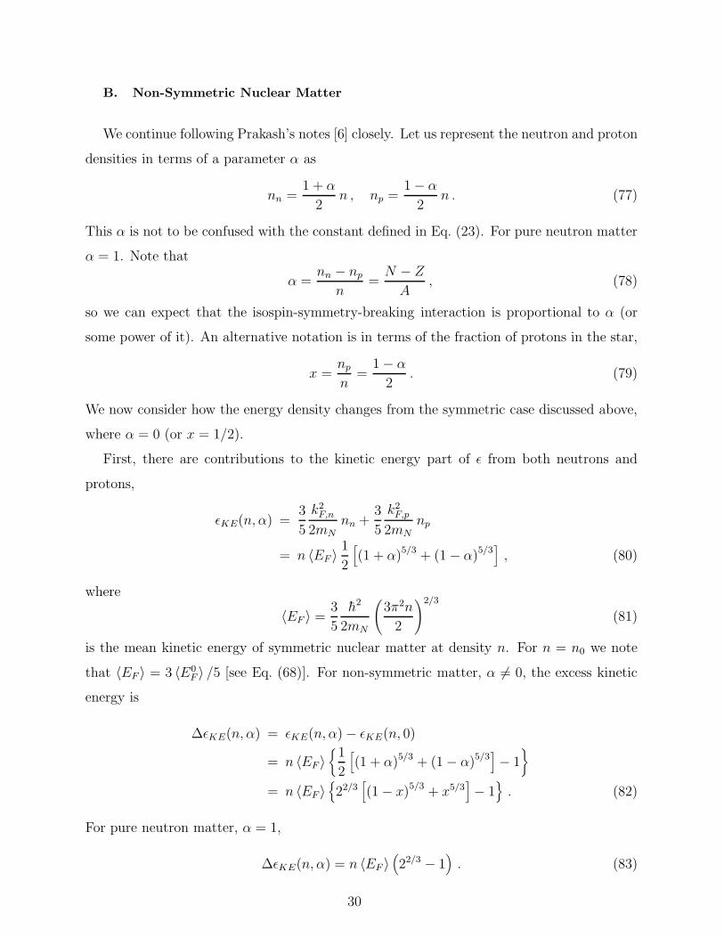
Figure 9 shows the energy per particle for pure neutron matter, E(n, 1) − mN , as a

function of u for the parameters of Eq. (75) and S0 = 30 MeV. In contrast with the α = 0

plot in Fig. 7, E(n, 1) ≥ 0 and is monotonically increasing. The plot looks almost quadratic

as a function of u. The dominant term at large u goes like uσ, and σ = 2.112 (for this case).

However, one might have expected a linear increase instead. We will return to this point in

Sec. 6.3.

31

E(n, α = 1) − mN

0.5 1 1.5 2u

20

40

60

FIG. 9: The average energy per neutron (less its rest mass), in MeV, for pure neutron matter, as

a function of u = n/n0. The parameters for this curve are for a nuclear compressibility K0 of 400

MeV.

Given the energy density, ǫ(n, α) = n0uE(n, α), the corresponding pressure is, from Eq.

(13),

p(n, x) = ud

duǫ(n, α) − ǫ(n, α)

= p(n, 0) + n0α2

[

22/3 − 1

5

⟨

E0F

⟩ (

2u5/3 − 3u2)

+ S0u2

]

, (89)

where p(n, 0) is defined by Eq. (76). Figure 10 shows the dependence of the pure neutron

p(n, 1) and ǫ(n, 1) on u = n/n0, ranging from 0 to 10 times normal nuclear density. Both

functions increase smoothly and monotonically from u = 0. We hope the student would

wonder why the pressure becomes greater than the energy density around u = 6. Why

doesn’t it go like a relativistic nucleon gas, p = ǫ/3? (Hint: check the assumptions.)

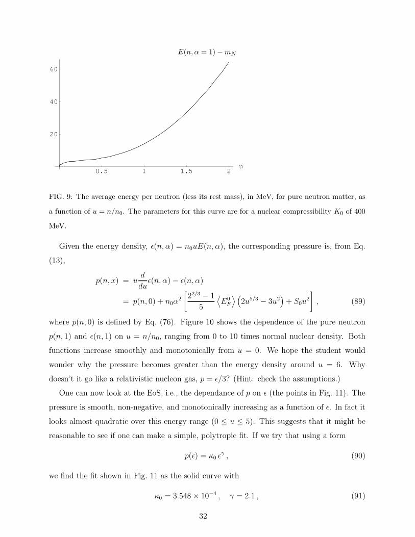
One can now look at the EoS, i.e., the dependance of p on ǫ (the points in Fig. 11). The

pressure is smooth, non-negative, and monotonically increasing as a function of ǫ. In fact it

looks almost quadratic over this energy range (0 ≤ u ≤ 5). This suggests that it might be

reasonable to see if one can make a simple, polytropic fit. If we try that using a form

p(ǫ) = κ0 ǫγ , (90)

we find the fit shown in Fig. 11 as the solid curve with

κ0 = 3.548 × 10−4 , γ = 2.1 , (91)

32

p and ǫ versus u

2 4 6 8 10u

2000

4000

6000

8000

FIG. 10: The pressure (dashed curve) and energy density (solid) for pure neutron matter, as a

function of u = n/n0. Units for the y-axis are MeV/fm3. This curve uses parameters based on a

nuclear compressibility K0 = 400 MeV.

where κ0 has appropriate units so that p and ǫ are in MeV/fm3. (We simply guessed and

set γ to that value.)

This polytrope can now be used in solving the TOV equation for a pure neutron star with

nuclear interactions. Alternatively, one might solve for the structure by using the functional

forms from Eq. (86), multiplied by n, and Eq. (89) directly. We defer that for a bit, since

it would be a good idea to first find an EoS which doesn’t violate causality, a basic tenet of

special relativity.

C. Does the Speed of Sound Exceed That of Light?

What is the speed of sound in nuclear matter? Starting from the elementary formula for

the square of the speed of sound in terms of the bulk modulus [27], one can show that

(

cs

c

)2

=B

ρc2=

dp

dǫ=

dp/dn

dǫ/dn. (92)

To satisfy relativistic causality we must require that the sound speed does not exceed that

of light. This can happen when the density becomes very large, i.e., when u → ∞. For the

simple model of nuclear interactions presented in the last section, the dominant terms at

large u in p and ǫ are those going like uσ+1. Thus, from Eq. (86), multiplied by n, and Eq.

33

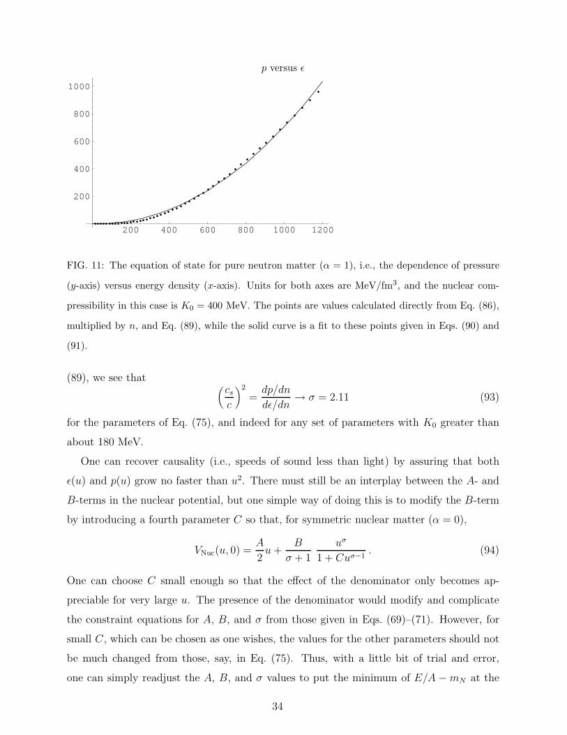
p versus ǫ

200 400 600 800 1000 1200

200

400

600

800

1000

FIG. 11: The equation of state for pure neutron matter (α = 1), i.e., the dependence of pressure

(y-axis) versus energy density (x-axis). Units for both axes are MeV/fm3, and the nuclear com-

pressibility in this case is K0 = 400 MeV. The points are values calculated directly from Eq. (86),

multiplied by n, and Eq. (89), while the solid curve is a fit to these points given in Eqs. (90) and

(91).

(89), we see that(

cs

c

)2

=dp/dn

dǫ/dn→ σ = 2.11 (93)

for the parameters of Eq. (75), and indeed for any set of parameters with K0 greater than

about 180 MeV.

One can recover causality (i.e., speeds of sound less than light) by assuring that both

ǫ(u) and p(u) grow no faster than u2. There must still be an interplay between the A- and

B-terms in the nuclear potential, but one simple way of doing this is to modify the B-term

by introducing a fourth parameter C so that, for symmetric nuclear matter (α = 0),

VNuc(u, 0) =A

2u +

B

σ + 1

uσ

1 + Cuσ−1. (94)

One can choose C small enough so that the effect of the denominator only becomes ap-

preciable for very large u. The presence of the denominator would modify and complicate

the constraint equations for A, B, and σ from those given in Eqs. (69)–(71). However, for

small C, which can be chosen as one wishes, the values for the other parameters should not

be much changed from those, say, in Eq. (75). Thus, with a little bit of trial and error,

one can simply readjust the A, B, and σ values to put the minimum of E/A − mN at the

34

right position (n0) and depth (BE), hoping that the resulting value of the (poorly known)

compressibility K0 remains sensible.

In our calculations we chose C = 0.2 and started the hand search with the K0 = 400

MeV parameters in Eq. (75). We found that, by fiddling only with B and σ, we could re-fit

n0 and B with only small changes,

B = 65.39 → 83.8 MeV , σ = 2.11 → 2.37 , (95)

somewhat larger than before. For these new values of B and σ, A changes from -122.2 MeV

to -136.7 MeV, and K0 from 400 to 363.2 MeV. That is, it remains a reasonable nuclear

model.

One can now proceed as in the last section to get ǫ(n, α), p(n, α), and the EoS, p(ǫ, α).

The results are not much different from those shown in the figures of the previous sub-

section. This time we decided to live with a quadratic fit for the EoS for pure neutron

matter, finding

p(ǫ, 1) = κ0ǫ2 , κ0 = 4.012 × 10−4 . (96)

This is not much different from before, Eq. (91). Somewhat more useful for solving the TOV

equation is to express ǫ in terms of p,

ǫ(p) = (p/κ0))1/2 . (97)

D. Pure Neutron Star with Nuclear Interactions

Having laid all this groundwork, the student can now proceed to solve the TOV equations

as before for a pure neutron star, using the fit for ǫ(p) found in the previous sub-section.

It is, once again, useful to convert from the units of MeV/fm3 to ergs/cm3 to M⊙/km3 and

dimensionless p and ǫ. By now the student has undoubtedly grown quite accustomed to

that procedure.

ǫ(p) = (κ0ǫ0)−1/2p1/2 = A0p

1/2 , A0 = 0.8642 , (98)

where this time we defined

ǫ0 =m4

nc5

3π2h3 . (99)

With this, the constant α that occurs on the right-hand side of the TOV equation, Eq. (22),

is α = A0R0 = 1.276 km. The constant for the mass equation, Eq. (25), is β = 0.03265,

again in units of 1/km3.

35

M(R)

5 10 15 20 25

0.5

1

1.5

2

2.5

FIG. 12: The mass M and radius R for pure neutron stars using an EoS which contains nucleon-

nucleon interactions. Only those stars to the right of the maximum are stable against gravitational

collapse. Compare this graph with that in Fig. 6 which is based on a non-interacting Fermi gas

model for the EoS.

Now proceeding as before, one can solve the coupled TOV equations for p(r) and M(r)

for various initial central pressures, p(0). We don’t exhibit here plots of the solutions, as

they look very similar to those for the Fermi gas EoS, Fig. 5.

More interesting is to solve for a range of initial p(0)’s, generating, as before, a mass M

versus radius R plot which now includes nucleon-nucleon interactions (Fig. 12). The effect

of the nuclear potential is enormous, on comparing with the Fermi gas model predictions

for M vs. R shown in Fig. 6. The maximum star mass this time is about 2.3 M⊙, rather

than 0.8 M⊙. The radius for this maximum mass star is about 13.5 km, somewhat larger

than the Fermi gas model radius of 11 km. The large value of maximum M is a reflection

of the large value of nuclear (in)compressibility K0 = 363 MeV. The more incompressible

something is, the more mass it can support. Had we fit to a smaller value of K0 we would

have gotten a smaller maximum mass.

E. What About a Cosmological Constant?

We do not know (either) if there is one, but there are definite indications that a great

part of the make-up of our universe is something called “Dark Energy” [28]. This conclusion

36

comes about because we have recently learned that something, at the present time, is causing

the universe to be accelerating, instead of slowing down (as would be expected after the Big

Bang).

One way (of several) to interpret this dark energy is as Einstein’s cosmological constant,

which contributes a term Λgµν to the right-hand side of Einstein’s field equation, the basic

equation of general relativity. The most natural value for Λ would be zero, but that may

not be the way the world is. If Λ is non-zero, it is nonetheless surprisingly small.

What would the effect of a non-zero cosmological constant be for the structure of a

neutron star? It turns out that the only modification to the TOV equation [29] is in the

correction factor[

1 +4πr3p(r)

M(r)c2

]

→[

1 +4πr3p(r)

M(r)c2− Λr3

2GM(r)

]

. (100)

So, we encourage the student to, first, understand the units of Λ and then to see what values

for it might affect the structure of a typical neutron star.

VII. CONCLUSIONS

The materials we have described in this paper would be quite suitable as an undergrad-

uate thesis or special topics course accessible to a junior or senior physics major. It is a

topic rich in the subjects the student will have covered in his or her courses, ranging from

thermodynamics to quantum statistics to nuclear physics.

The major emphasis in such a project is on constructing a (simple) equation of state.

This is needed to be able to solve the non-linear structure equations. Solving those equations

numerically, of course, develops the student’s computational skills. Along the way, however,

he or she will also learn some of the lore regarding degenerate stars, e.g., white dwarfs and

neutron stars. And, in the latter case, the student will also come to appreciate the relative

importance of special and general relativity.

VIII. ACKNOWLEDGMENTS

We thank M. Prakash, T. Buervenich, and Y.-Z. Qian for their helpful comments and for

reading drafts of this paper. We would also like to acknowledge comments and suggestions

made by an anonymous referee. This research is supported in part by the Department of

37

Energy under contract W-7405-ENG-36.

[1] It is widely beleived that neutron stars were proposed by Lev Landau in 1932, very soon after

the neutron was discovered (although we are not aware of any documented proof of this).

In 1934 Fritz Zwicky and Walter Baade speculated that they might be formed in Type II

supernova explosions, which is now generally accepted as true.

[2] An on-line catalog of pulsars can be found at http:/pulsar.princeton.edu.

[3] An intermediate-level on-line tutorial on the physics of pulsars can be found at

http://www.jb.man.ac.uk/research/pulsar. This tutorial follows the book by Andrew G. Lyne

and Francis Graham-Smith, Pulsar Astronomy, 2nd. ed., Cambridge University Press, 1998.

[4] R. C. Tolman, Phys. Rev. 55, 364 (1939); J. R. Oppenheimer and G. M. Volkov, Phys. Rev.

55, 374 (1939).

[5] Steven Weinberg, Gravitation and Cosmology, John Wiley & Sons, Inc., New York, 1972,

Chapter 11.

[6] M. Prakash, lectures delivered at the Winter School on “The Equation of State of Nuclear

Matter,” Puri, India, January 1994, esp. Chapter 3, Equation of State. These notes are pub-

lished in “The Nuclear Equation of State”, ed. by A. Ausari and L. Satpathy, World Scientific

Publishing Co., Singapore, 1996.

[7] If you are a mentor for such a student, you may want to see some of the Mathematica and

MathCad files we developed along our path of discovery. Send e-mail to the first author

convincing him that you are such a mentor, and he will direct you to a web page from which

they can be downloaded. The idea behind this misdirection is that the student will learn more

by doing the programming himself.

[8] R. Balian and J.-P. Blaizot, “Stars and Statistical Physics: A Teaching Experience,” Am. J.

Phys. 67, (12) 1189 (1999).

[9] S. L. Shapiro and S. A. Teukolsky, Black Holes, White Dwarfs and Neutron Stars: The Physics

of Compact Objects, Wiley-Interscience, 1983.

[10] We apologize to readers who are enthusiasts of SI units, but the first author was raised on

CGS units. Actually, we strongly feel that by the time a physics student is at this level, he or

she ought to be comfortable in switching from one system of units to another.

38

[11] A discussion of how to solve these equations (using conventional programming languages) is

given in S. Koonin, Computational Physics, Benjamin-Cummings Publishing, 1986.

[12] For more details on white dwarfs, NASA provides a useful web page at

http://imagine.gsfc.nasa.gov/docs/science/know l1/dwarfs.html.

[13] This maximum mass of 1.4 M⊙ is usually referred to as the Chandrasekhar limit. See S. Chan-

drasekhar’s 1983 Nobel Prize lecture, http://www.nobel.se/physics/laureates/1983/. For more

detail see his treatise, An Introduction to the Study of Stellar Structure, Dover Publications,

New York, 1939.

[14] Mathematica is a software product of Wolfram Research, Inc., (see web page at http://www.-

wolfram.com), and its use is described by S. Wolfram in The Mathematica Book, Fourth Ed.,

Cambridge University Press, Cambridge, England, 1999. However, whenever we use the phrase

“using Mathematica,” we really mean using whatever package one has available or is familiar

with, be it Maple, MathCad, or whatever. We did almost all of the numerical/symbolic work

that we describe in this paper in Mathematica, but some of its notebooks were duplicated in

MathCad, just to be sure it could be done there as well.

[15] Enough of these explicit flags! Most of the equations from here on present challenges for the

student to work through.

[16] For the Newtonian case, a polytropic EoS also allows for a somewhat more analytic solution

in terms of Lane-Emden functions. See Weinberg, op. cit., Sec. 11.3, or C. Flynn, Lectures on

Stellar Physics, especially lectures 4 and 5, at http://www.astro.utu.fi∼cflynn/Stars/.

[17] Despite the appearance of the 4πǫ0, the astute student will not be lulled into thinking that this

factor has anything to do with a Coulomb potential or the dielectric constant of the vacuum.

[18] Note that the right-hand side of Eq. (22) is negative (for positive p), so p(r) must fall mono-

tonically from p(0).

[19] We leave this for the student to figure out, except for the following hint: Use an if statement

if necessary.

[20] This fit is least accurate (≈ 2%) at very low values of kF . However, this is where the pure

neutron approximation itself is least accurate. The surface of a neutron star is likely made of

elements like iron. A fictional account of what life might be like on such a surface can be found

in Robert Forward’s Dragon’s Egg, first published in 1981 by Del Rey Publishing, republished

in 2000.

39

[21] See Weinberg, op. cit., Sec. 11.2.

[22] Because it is almost non-interacting with nuclear matter, a neutrino tends to escape from the

neutron star. This is the major cooling mechanism as the neutron star is being formed in a

supernova explosion. George Gamow named this the URCA process, after a Brazilian casino

where people lost a lot of money.

[23] Does the student know how to put all the factors of c back into ǫ0 so as to re-write this for

CGS units?

[24] See, e.g., J. M. Blatt and V. F. Weisskopf, Theoretical Nuclear Physics, John Wiley & Sons,

1952, Chap. 6, Sec. 2.

[25] The reason for the “(in)” is because a materials physicist might rather define compressibility

as χ = −(1/V )(∂V/∂p) = −(1/n)(dp/dn)−1.

[26] Folks interested in RHIC physics might want to, however. (RHIC stands for “Relativis-

tic Heavy Ion Collider,” an accelerator at the Brookhaven National Laboratory which is

studying reactions like Au nuclei striking each other at center of mass energies around 200

GeV/nucleon.)

[27] See, e.g., Hugh Young, University Physics, 8th ed., Addison-Wesley, Reading MA, 1992, Sec.

19-5, Speed of a Longitudinal Wave.

[28] See, e.g., P. J. E. Peebles and Bharat Ratra, Rev. Mod. Phys. 75, 599 (2003)

[29] W. Y. Pauchy Hwang, private communication.

40