neurogenesis-inspired dictionary learning: … · neurogenesis-inspired dictionary learning...

Neurogenesis-Inspired Dictionary Learning

NEUROGENESIS-INSPIRED DICTIONARY LEARNING:ONLINE MODEL ADAPTION IN A CHANGING WORLD

Sahil GargThe Department of Computer Science, University of Southern California, Los Angeles, CA [email protected]

Irina Rish, Guillermo Cecchi, Aurelie LozanoIBM Thomas J. Watson Research Center, Yorktown Heights, NY USA{rish, gcecchi, aclozano}@us.ibm.com

ABSTRACT

In this paper, we focus on online representation learning in non-stationary envi-ronments which may require continuous adaptation of model’s architecture. Wepropose a novel online dictionary-learning (sparse-coding) framework which in-corporates the addition and deletion of hidden units (dictionary elements), and isinspired by the adult neurogenesis phenomenon in the dentate gyrus of the hip-pocampus, known to be associated with improved cognitive function and adapta-tion to new environments. In the online learning setting, where new input instancesarrive sequentially in batches, the “neuronal birth” is implemented by adding newunits with random initial weights (random dictionary elements); the number ofnew units is determined by the current performance (representation error) of thedictionary, higher error causing an increase in the birth rate. “Neuronal death” isimplemented by imposing l1/l2-regularization (group sparsity) on the dictionarywithin the block-coordinate descent optimization at each iteration of our onlinealternating minimization scheme, which iterates between the code and dictionaryupdates. Finally, hidden unit connectivity adaptation is facilitated by introduc-ing sparsity in dictionary elements. Our empirical evaluation on several real-lifedatasets (images and language) as well as on synthetic data demonstrates that theproposed approach can considerably outperform the state-of-art fixed-size (non-adaptive) online sparse coding of Mairal et al. (2009) in the presence of non-stationary data. Moreover, we identify certain properties of the data (e.g., sparseinputs with nearly non-overlapping supports) and of the model (e.g., dictionarysparsity) associated with such improvements.

1 INTRODUCTION

The ability to adapt to a changing environment is essential for successful functioning in both naturaland artificial intelligent systems. In human brains, adaptation is achieved via neuroplasticity, whichtakes different forms, including synaptic plasticity, i.e. changing connectivity strength among neu-rons, and neurogenesis, i.e. the birth and maturation of new neurons (accompanied with the death ofsome new or old neurons). Particularly, adult neurogenesis (Kempermann, 2006) (i.e., neurogenesisin the adult brain) in the dentate gyrus of the hippocampus is associated with improved cognitivefunctions such as pattern separation (Sahay et al., 2011), and is often implicated as a “candidatemechanism for the specific dynamic and flexible aspects of learning” (Stuchlik, 2014).

In the machine-learning context, synaptic plasticity is analogous to parameter tuning (e.g., learningneural net weights), while neurogenesis can be viewed as an online model selection via addition(and deletion) of hidden units in specific hidden-variable models used for representation learning(where hidden variables represent extracted features), from linear and nonlinear component anal-ysis methods such as PCA, ICA, sparse coding (dictionary learning), nonlinear autoencoders, todeep neural nets and general hidden-factor probabilistic models. However, optimal model selectionin large-scale hidden-variable models (e.g., adjusting the number of layers, hidden units, and their

1

arX

iv:1

701.

0610

6v2

[cs

.LG

] 1

9 Fe

b 20

17


connectivity), is intractable due to enormous search space size. Growing a model gradually can be amore feasible alternative; after all, every real brain’s “architecture” development process starts witha single cell. Furthermore, the process of adapting the model’s architecture to dynamically changingenvironments is necessary for achieving a lifelong, continual learning. Finally, an online approachto dynamically expanding and contracting model’s architecture can serve as a potentially more ef-fective alternative to the standard off-line model selection (e.g., MDL-based off-line sparse coding(Ramirez & Sapiro, 2012)), as well as to the currently popular network compression (distillation)approaches (Hinton et al., 2015; Srivastava et al., 2014; Ba & Caruana, 2014; Bucilu et al., 2006),where a very large-scale architecture, such as a deep neural network with millions of parameters,must be first selected in ad-hoc ways and trained on large amounts of data, only to be compressedlater to a more compact and simpler model with similarly good performance; we hypothesize thatadaptive growth and reduction of the network architecture is a viable alternative to the distillationapproach, although developing such an alternative remains the topic of further research.

In this paper, we focus on dictionary learning, a.k.a. sparse coding (Olshausen & Field, 1997; Kreutz-Delgado et al., 2003; Aharon et al., 2006; Lee et al., 2006) – a representation learning approachwhich finds a set of basis vectors (atoms, or dictionary elements) and representations (encodings)of the input samples as sparse linear combinations of those elements1. More specifically, our ap-proach builds upon the computationally efficient online dictionary-learning method of Mairal et al.(2009), where the data samples are processed sequentially, one at a time (or in small batches). Onlineapproaches are particularly important in large-scale applications with millions of potential trainingsamples, where off-line learning can be infeasible; furthermore, online approaches are a naturalchoice for building systems capable of continual, lifelong learning.

Herein, we propose a novel online dictionary learning approach inspired by adult neurogenesis,which extends the state-of-art method of Mairal et al. (2009) to nonstationary environments by in-corporating online model adaption, i.e. the addition and deletion of dictionary elements (i.e., hiddenunits) in response to the dynamically changing properties of the input data2. More specifically, ateach iteration of online learning (i.e., for every batch of data samples), we add a group of randomdictionary elements (modeling neuronal birth), where the group size depends on the current repre-sentation error, i.e. the mismatch between the new input samples and their approximation based onthe current dictionary: higher error triggers more neurogenesis. The neuronal death, which involvesremoving “useless” dictionary elements, is implemented as an l1/l2 group-sparsity regularization;this step is essential in neurogenesis-inspired learning, since it reduces a potentially uncontrolledgrowth of the dictionary, and helps to avoid overfitting (note that neuronal death is also a naturalpart of the adult neurogensis process, where neuronal survival depends on multiple factors, includ-ing the complexity of a learning environment (Kempermann, 2006)). Moreover, we introduce spar-sity in dictionary elements, which reflects sparse connectivity between hidden units/neurons andtheir inputs; this is a more biologically plausible assumption than the fully-connected architectureof standard dictionary learning, and it also works better in our experiments. Thus, adaptation in ourmodel involves not only the addition/deletion of the elements, but adapting their connectivity aswell.

We demonstrate on both simulated data and on two real-life datasets (natural images and languageprocessing) that, in presence of a non-stationary input, our approach can significantly outperformnon-adaptive, fixed-dictionary-size online method of Mairal et al. (2009). Moreover, we identify cer-tain data properties and parameter settings associated with such improvements. Finally, we demon-strate that the novel approach not only improves the representation accuracy, but also can boost theclassification accuracy based on the extracted features.

Note that, although the group-sparsity constraint enforcing deletion of some dictionary elementswas introduced earlier in the group-sparse coding method of Bengio et al. (2009), it was only im-plemented and tested in the off-line rather than online setting, and, most importantly, it was not ac-

1Note that the corresponding neural network interpretation of sparse coding framework is a (single-hidden-layer) linear autoencoder with sparsity constraints: the hidden units are associated with dictionary elements,each element represented by a weight vector associated with unit’s outgoing links in the output layer, and thesparse vector of hidden unit activations corresponding to the encoding of an input.

2An early version of our neurogenetic online dictionary learning approach was presented as a poster at the2011 Society for Neuroscience meeting (Rish et al., 2011), although it did not appear before as a peer-reviewedpublication.

2


companied by the neurogenesis. On the other hand, while some prior work considered online nodeaddition in hidden-variable models, and specifically, in neural networks, from cascade correlations(Fahlman & Lebiere, 1989) to the recent work by Draelos et al. (2016a;b), no model pruning wasincorporated in those approaches in order to balance the model expansion. Overall, we are not awareof any prior work which would propose and systematically evaluate, empirically and theoretically, adynamic process involving both addition and deletion of hidden units in the online model selectionsetting, either in sparse coding or in a neural network setting.

To summarize, the main contributions of this paper are as follows:

• we propose a novel online model-selection approach to dictionary learning3, inspired bythe adult neurogenesis phenomenon; our method significantly outperforms the state-of-artbaseline, especially in non-stationary settings;• we perform an extensive empirical evaluation, on both synthetic and real data, in order

to identify the conditions when the proposed adaptive approach is most beneficial, bothfor data reconstruction and for classification based on extracted features; we conclude thatthese conditions include a combination of sparse dictionary elements (and thus a morebiologically plausible sparse network connectivity as opposed to fully connected units),accompanied by sufficiently dense codes;

• furthermore, we provide an intuitive discussion, as well as theoretical analysis of certaincombinations of the input data properties and the algorithm’s parameters when the pro-posed approach is most beneficial;

• from the neuroscientific perspective, we propose a computational model which supportsearlier empirical observations indicating that adult neurogenesis is particularly beneficialin changing environments, and that certain amount of neuronal death, which accompaniesthe neuronal birth, is an important component of an efficient neurogenesis process;

• overall, to the best of our knowledge, we are the first to perform an in-depth evaluationof the interplay between the birth and death of hidden units in the context of online modelselection in representation learning, and, more specifically, in online dictionary learning.

This paper is organized as follows. In Sec. 2, we summarize the state-of-art non-adaptive (fixed-size) online dictionary learning method of Mairal et al. (2009). Thereafter, in Sec. 3, we describeour adaptive online dictionary learning algorithm. In Sec. 4, we present our empirical results on bothsynthetic and real datasets, including images and language data. Next, in Sec. 5, we provide sometheoretical, as well as an intuitive analysis of settings which can benefit most from our approach.Finally, we conclude with a summary of our contributions in Sec. 6. The implementation details ofthe algorithms and additional experimental results are described in the Appendix.

2 BACKGROUND ON DICTIONARY LEARNING

Traditional off-line dictionary learning (Olshausen & Field, 1997; Aharon et al., 2006; Lee et al.,2006) aims at finding a dictionary D ∈ Rm×k, which allows for an accurate representation of atraining data set X = {x1, · · · ,xn ∈ Rm}, where each sample xi is approximated by a linearcombination xi ≈ Dαi of the columns of D, called dictionary elements {d1, · · · ,dk ∈ Rm}.Here αi is the encoding (code vector, or simply code) of xi in the dictionary. Dictionary learningis also referred to as sparse coding, since it is assumed that the code vectors are sparse, i.e. have arelatively small number of nonzeros; the problem is formulated as minimizing the objective

fn(D) =1

n

n∑

i=1

1

2||xi −Dαi||22 + λc||αi||1 (1)

where the first term is the mean square error loss incurred due to approximating the input samplesby their representations in the dictionary, and the second term is the l1-regularization which enforcesthe codes to be sparse. The joint minimization of fn(D) with respect to the dictionary and codes isnon-convex; thus, a common approach is alternating minimization involving convex subproblems offinding optimal codes while fixing a dictionary, and vice versa.

3The Matlab code is available at https://github.com/sgarg87/neurogenesis_inspired_dictionary_learning.

3


However, the classical dictionary learning does not scale to very large datasets; moreover, it is notimmediately applicable to online learning from a continuous stream of data. The online dictionarylearning (ODL) method proposed by Mairal et al. (2009) overcomes both of these limitations, andserves as a basis for our proposed approach, presented in Alg. 1 in the next section. While the high-lighted lines in Alg. 1 represent our extension of ODL , the non-highlighted ones are common to bothapproaches, and are discussed first. The algorithms start with some dictionary D0, e.g. a randomlyinitialized one (other approaches include using some of the inputs as dictionary elements (Mairalet al., 2010; Bengio et al., 2009)). At each iteration t, both online approaches consider the next inputsample xt (more generally, a batch of samples) as in the step 3 of Alg. 1 and compute its sparsecode αt by solving the LASSO (Tibshirani, 1996) problem (the step 4 in Alg. 1), with respect to thecurrent dictionary. In Alg. 1, we simply use D instead of D(t) to simplify the notation. Next, thestandard ODL algorithm computes the dictionary update, D(t), by optimizing the surrogate objec-tive function ft(D) which is defined just as the original objective in eq. (1), for n = t, but with oneimportant difference: unlike the original objective, where each code αi for sample xi is computedwith respect to the same dictionary D, the surrogate function includes the codes α1,α2, · · · ,αt

computed at the previous iterations, using the dictionaries D(0), ...,D(t−1), respectively; in otherwords, it does not recompute the codes for previously seen samples after each dictionary update.This speeds up the learning without worsening the (asymptotic) performance, since the surrogateobjective converges to the original one in (1), under certain assumptions, including data stationarity(Mairal et al., 2009). Note that, in order to prevent the dictionary entries from growing arbitrarilylarge, Mairal et al. (2009; 2010) impose the norm constraint, i.e. keep the columns of D within theconvex set C = {D ∈ Rm×k s.t. ∀j dT

j uj ≤ 1}. Then the dictionary update step computesD(t) = argminD∈C ft(D), ignoring l1-regularizer over the code which is fixed at this step, as

arg minD∈C

1

t

t∑

i=1

1

2||xi −Dαi||22 = arg min

D∈C1

2Tr(DTDA)− Tr(DTB), (2)

where A =∑t

i=1 αiαTi and B =

∑ti=1 xiα

Ti are the “bookkeeping” matrices (we also call them

“memories” of the model), compactly representing the input samples and encoding history. At eachiteration, once the new input sample xi is encoded, the matrices are updated as A ← A + αtα

Tt

and B ← B + xtαTt (see the step 11 of Alg. 1). In (Mairal et al., 2009; 2010), a block coordinate

descent is used to optimize the convex objective in eq. 2; it iterates over the dictionary elements in afixed sequence, optimizing each while keeping the others fixed as shown in eq. (3) (essentially, thesteps 14 and 17 in Alg. 1; the only difference is that our approach will transform uj into wj in orderto impose additional regularizer before computing step 17), until convergence.

uj ←bj −

∑k 6=j dkajk

ajj; dj ←

uj

max(1, ||uj ||2)(3)

Herein, when the off-diagonal entries ajk in A are as large as the diagonal ajj , the dictionary ele-ments get “tied” to each other, playing complementary roles in the dictionary, thereby constrainingthe updates of each other.

It is important to note that, for the experiment settings where we consider dictionary elements tobe sparse in our algorithm NODL (discussed next in Sec. 3), we will actually use as a baselinealgorithm a modified version of the fixed-size ODL, which allows for sparse dictionary elements, i.e.includes the sparsification step 15 in Alg. 1, thus optimizing the following objective in dictionaryupdate step instead of the one in eq. (2):

arg minD∈C

1

t

t∑

i=1

1

2||xi −Dαi||22 +

∑

j

λj ||dj ||1. (4)

From now on, ODL will refer to the above extended version of the fixed-size method of Mairalet al. (2009) wherever we have sparsity in dictionary elements (otherwise, the standard method ofMairal et al. (2009) is the baseline); in our experiments, dictionary sparsity of both the baselineand the proposed method (discussed in the next section) will be matched. Note that Mairal et al.(2010) mention that the convergence guaranties for ODL hold even with the sparsity constraints ondictionary elements.

4


3 OUR APPROACH: NEUROGENIC ONLINE DICTIONARY LEARNING (NODL)

Our objective is to extend the state-of-art online dictionary learning, designed for stationary inputdistributions, to a more adaptive framework capable of handling nonstationary data effectively, andlearning to represent new types of data without forgetting how to represent the old ones. Towards thisend, we propose a novel algorithm, called Neurogenetic Online Dictionary Learning (see Alg. 1),which can flexibly extend and reduce a dictionary in response to the changes in an input distribution,and possibly to the inherent representation complexity of the data. The main changes, as compared tothe non-adaptive, fixed-dictionary-size algorithm of Mairal et al. (2009), are highlighted in Alg. 1;the two parts involve (1) neurogenesis, i.e. the addition of dictionary elements (hidden units, or“neurons”) and (2) the death of old and/or new elements which are “less useful” than other elementsfor the task of data reconstruction.

At each iteration in Alg. 1, the next batch of samples is received and the corresponding codes, inthe dictionary, are computed; next, we add kn new dictionary elements sampled at random fromRm (i.e., kn random linear projections of the input sample). The choice of the parameter kn isimportant; one approach is to tune it (e.g., by cross-validation), while another is to adjust it dynam-ically, based on the dictionary performance: e.g., if the environment is changing, the old dictionarymay not be able to represent the new input well, leading to decline in the representation accuracy,which triggers neurogenesis. Herein, we use as the performance measure the Pearson correlationbetween a new sample and its representation in the current dictionary r(xt,D

(t−1)αt), i.e. denotedas pc(xt,D

(t−1),αt) (for a batch of data, the average over pc(.) is taken). If it drops below a certainpre-specified threshold γ (where 0 ≪ γ ≤ 1), the neurogenesis is triggered (the step 5 in Alg. 1).The number kn of new dictionary elements is proportional to the error 1− pc(·), so that worse per-formance will trigger more neurogenesis, and vice versa; the maximum number of new elements isbounded by ck (the step 6 in Alg. 1). We refer to this approach as conditional neurogenesis as itinvolves the conditional birth of new elements. Next, kn random elements are generated and addedto the current dictionary (the step 7), and the memory matrices A,B are updated, respectively, toaccount for larger dictionary (the step 8). Finally, the sparse code is recomputed for xt (or, all thesamples in the current batch) with respect to the extended dictionary (the step 9).

The next step is the dictionary update, which uses, similarly to the standard online dictionary learn-ing, the block-coordinate descent approach. However, the objective function includes additionalregularization terms, as compared to (2):

D(t)=arg minD∈C

1

t

t∑

i=1

1

2||xi −Dαi||22 + λg

∑

j

||dj ||2 +∑

j

λj ||dj ||1. (5)

The first term is the standard reconstruction error, as before. The second term, l1/l2-regularization,promotes group sparsity over the dictionary entries, where each group corresponds to a column, i.e.a dictionary element. The group-sparsity (Yuan & Lin, 2006) regularizer causes some columns inD to be set to zero (i.e. the columns less useful for accurate data representation), thus effectivelyeliminating the corresponding dictionary elements from the dictionary (“killing” the correspondinghidden units). As it was mentioned previously, Bengio et al. (2009) used the l1/l2-regularizer indictionary learning, though not in online setting, and without neurogenesis.

Finally, the third term imposes l1-regularization on dictionary elements thus promoting sparse dic-tionary, besides the sparse coding. Introducing sparsity in dictionary elements, corresponding to thesparse connectivity of hidden units in the neural net representation of a dictionary, is motivated byboth their biological plausibility (neuronal connectivity tends to be rather sparse in multiple brainnetworks), and by the computational advantages this extra regularization can provide, as we observelater in experiments section (Sec. 4).

As in the original algorithm of Mairal et al. (2009), the above objective is optimized by the block-coordinate descent, where each block of variables corresponds to a dictionary element, i.e., a columnin D; the loop in steps 12-19 of the Alg. 1 iterates until convergence, defined by the magnitude ofchange between the two successive versions of the dictionary falling below some threshold. Foreach column update, the first and the last steps (the steps 14 and 17) are the same as in the originalmethod of Mairal et al. (2009), while the two intermediate steps (the steps 15 and 16) are implement-ing additional regularization. Both steps 15 and 16 (sparsity and group sparsity regularization) are

5


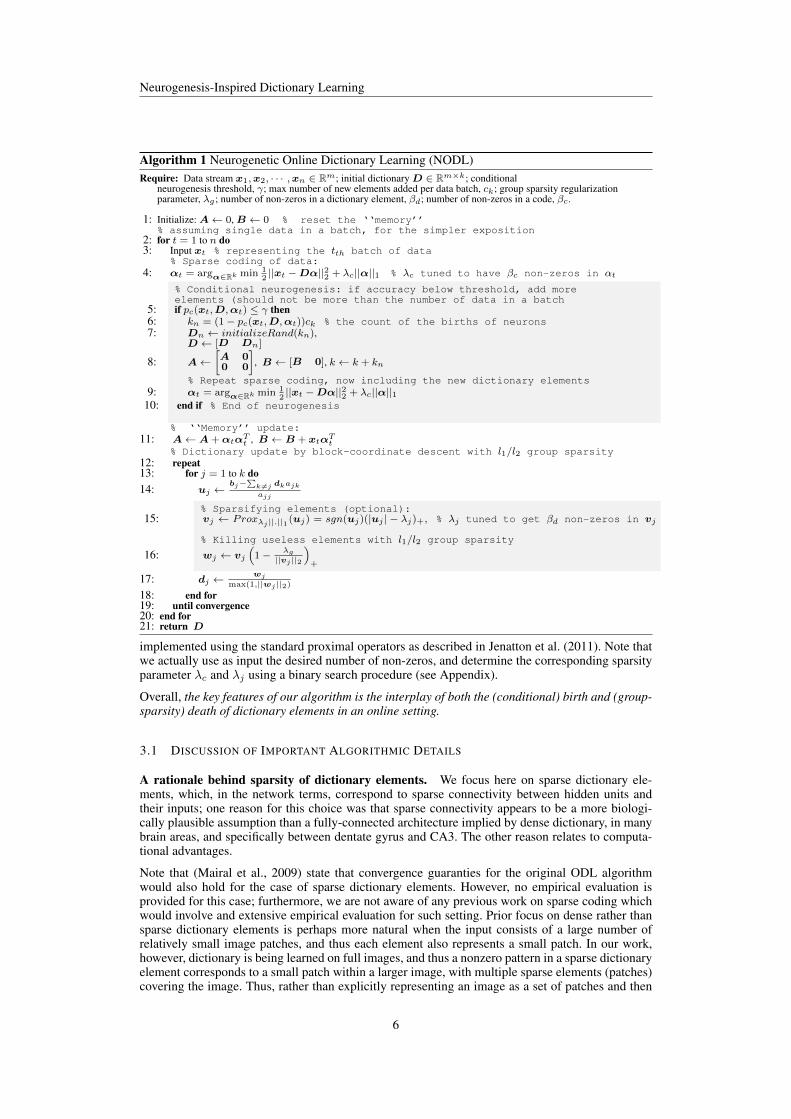
Algorithm 1 Neurogenetic Online Dictionary Learning (NODL)Require: Data stream x1,x2, · · · ,xn ∈ Rm; initial dictionary D ∈ Rm×k; conditional

neurogenesis threshold, γ; max number of new elements added per data batch, ck; group sparsity regularizationparameter, λg ; number of non-zeros in a dictionary element, βd; number of non-zeros in a code, βc.

1: Initialize: A← 0, B ← 0 % reset the ‘‘memory’’% assuming single data in a batch, for the simpler exposition

2: for t = 1 to n do3: Input xt % representing the tth batch of data

% Sparse coding of data:4: αt = argα∈Rk min 1

2||xt −Dα||22 + λc||α||1 % λc tuned to have βc non-zeros in αt

% Conditional neurogenesis: if accuracy below threshold, add moreelements (should not be more than the number of data in a batch

5: if pc(xt,D,αt) ≤ γ then6: kn = (1− pc(xt,D,αt))ck % the count of the births of neurons7: Dn ← initializeRand(kn),

D ← [D Dn]

8: A←[A 00 0

], B ← [B 0], k ← k + kn

% Repeat sparse coding, now including the new dictionary elements9: αt = argα∈Rk min 1

2||xt −Dα||22 + λc||α||1

10: end if % End of neurogenesis

% ‘‘Memory’’ update:11: A← A+αtαT

t , B ← B + xtαTt

% Dictionary update by block-coordinate descent with l1/l2 group sparsity12: repeat13: for j = 1 to k do14: uj ←

bj−∑

k 6=j dkajk

ajj

% Sparsifying elements (optional):15: vj ← Proxλj ||.||1 (uj) = sgn(uj)(|uj | − λj)+, % λj tuned to get βd non-zeros in vj

% Killing useless elements with l1/l2 group sparsity

16: wj ← vj

(1− λg

||vj ||2

)+

17: dj ← wj

max(1,||wj ||2)18: end for19: until convergence20: end for21: return D

implemented using the standard proximal operators as described in Jenatton et al. (2011). Note thatwe actually use as input the desired number of non-zeros, and determine the corresponding sparsityparameter λc and λj using a binary search procedure (see Appendix).

Overall, the key features of our algorithm is the interplay of both the (conditional) birth and (group-sparsity) death of dictionary elements in an online setting.

3.1 DISCUSSION OF IMPORTANT ALGORITHMIC DETAILS

A rationale behind sparsity of dictionary elements. We focus here on sparse dictionary ele-ments, which, in the network terms, correspond to sparse connectivity between hidden units andtheir inputs; one reason for this choice was that sparse connectivity appears to be a more biologi-cally plausible assumption than a fully-connected architecture implied by dense dictionary, in manybrain areas, and specifically between dentate gyrus and CA3. The other reason relates to computa-tional advantages.

Note that (Mairal et al., 2009) state that convergence guaranties for the original ODL algorithmwould also hold for the case of sparse dictionary elements. However, no empirical evaluation isprovided for this case; furthermore, we are not aware of any previous work on sparse coding whichwould involve and extensive empirical evaluation for such setting. Prior focus on dense rather thansparse dictionary elements is perhaps more natural when the input consists of a large number ofrelatively small image patches, and thus each element also represents a small patch. In our work,however, dictionary is being learned on full images, and thus a nonzero pattern in a sparse dictionaryelement corresponds to a small patch within a larger image, with multiple sparse elements (patches)covering the image. Thus, rather than explicitly representing an image as a set of patches and then

6


learning a dictionary of dense elements for accurate representation of such patches, a dictionary offull-image-size, but sparse dictionary elements can be used to implicitly represents an image as alinear combination of those elements, with possible overlap of non-zero pixels between elements;the non-zero pixels in a sparse element of a dictionary are learned automatically. Computationaladvantages of using sparse dictionaries are demonstrated in our experiment results (Sec. 4), whereclassifiers learned on top of representations extracted with sparse dictionaries yield smaller errors.

The memory matrix A and its properties. The matrix A keeps the “memory” of the encodingsαt for the previous data samples, in a sense, as it accumulates the sum of αtα

Tt matrices from

each iteration t. It turns out that the matrix A can have a significant effect on dictionary learningin both ODL and NODL algorithms. As it is pointed out in (Mairal et al., 2009), the quadraticsurrogate function in (2) is strictly convex with a lower-bounded Hessian A ensuring convergence toa solution. From the practical standpoint, when the matrix A has a high condition number (the ratioof the largest to smallest singular value in the singular value decomposition of a matrix), despiteits lower-bounded eigenvalues, the adaptation of a dictionary elements using the standard ODLalgorithm can be difficult, as we see in our experiments. Specifically, when the dictionary elementsare sparse, this effect is more pronounced, since the condition number of A becomes high dueto the complementary roles of sparse dictionary elements in the reconstruction process (see thecomparison of A from dense elements and sparse elements in 6(a) and 6(b), respectively). In suchscenarios, the submatrix of A corresponding to the new elements in a dictionary, added by ourNODL algorithm, can have a better condition number, leading to an improved adaptation of thedictionary.

Code Sparsity. Code sparsity is controlled by the parameter βc, the number of nonzeros, whichdetermines the corresponding regularization weight λc in step 4 of Alg. 1; note that λc is determinedvia binary search for each input sample separately, as shown in Algorithm 2, and thus may varyslightly for different instances given a fixed βc.

Selecting an appropriate level of code sparsity depends on the choice of other parameters, such as theinput batch size, sparsity of the dictionary elements, the extent of non-stationarity and complexityof the data, and so on. When the dictionary elements are themselves sparse, denser codes may bemore appropriate, since each sparse dictionary element represents only a relatively small subset ofimage pixels, and thus a large number of those subsets covering the whole image may be needed foran accurate input representation.

Interestingly, using very sparse codes in combination with non-sparse dictionary elements in thestandard ODL approach can sometimes lead to creation of “dead” (zero l2-norm) elements in thedictionary, especially if the input batch size is small. This is avoided by our NODL algorithm, sincesuch dead elements are implicitly removed via group sparsity at the dictionary update step, alongwith the “weak” (very small l2-norm) elements. Also, a very high code sparsity in combination withdense dictionary elements can lead to a significant decrease in the reconstruction accuracy for bothODL and our NODL when the online data stream is non-stationary. Such shortcomings were notencountered in (Mairal et al., 2009; 2010), where only stationary data streams were studied, both intheoretical and empirical results. On the other hand, high sparsity in dictionary elements does notseem to cause a degradation in the reconstruction accuracy, as long as the codes are not too sparse.

The choice and tuning of metric for conditional neuronal birth. In the “conditional birth” ap-proach described above, the number of new elements kn is determined based on the performance ofthe current dictionary, using the Pearson correlation between the actual and reconstructed data, forthe current batch. This is, of course, just one particular approach to measuring data nonstationarityand the need for adaptation, but we consider it a reasonable heuristic. Low reconstruction error in-dicates that the old dictionary is still capable of representing the new data, and thus less adaptationmight be needed, while a high error indicates that the data distribution might have changed, andtrigger neurogenesis in order to better adapt to a new environment. We choose the Pearson correla-tion as the measure of reconstruction accuracy since its value is easily interpretable, is always in therange [0, 1] (unlike, for example, the mean-square error), which simplifies tuning the threshold pa-rameter γ. Clearly, one can also try other interpretable metrics, such as, for example, the Spearmancorrelation.

7


Tuning parameters: group sparsity λg and others. The group sparsity regularization parameterλg controls the amount of removal (“death”) of elements in NODL : in step 16 of the Alg. 1, all ele-ments with l2-norm below λg (i.e., “weak” elements), are set to zero (“killed”). Since the dictionaryelements are normalized to have l2-norm less than one, we only need to consider λg ∈ [0, 1]. (Notethat the step of killing dictionary elements precedes the normalization step in the algorithm. Thus,the tuning of λg is affected by the normalization of the elements from the previous iteration.) Notethat increasing the sparsity of the dictionary elelments, i.e. decreasing βd (the number of nozeros indictionary elements) may require the corresponding reduction of λg , while an increase in the inputdimensionality m may also require an increase in the λg parameter. Tuning the rest of the parametersis relatively easy. Clearly, the batch size should be kept relatively small, and, ideally, not exceed the“window of stationarity” size in the data (however, the frequency of the input distribution changemay need to be also estimated from the data, and thus the batch size may need to be tuned adaptively,which is outside of the scope of this paper). Mairal et al. (2009) suggest to use a batch size of 256 intheir experiments while getting similar performance with values 128 and 512. As to the maximumnumber of new elements ck added at each iteration, it is reasonable to keep it smaller than the batchsize.

4 EXPERIMENTS

We now evaluate empirically the proposed approach, NODL, against ODL, the standard (non-adaptive) online dictionary learning of Mairal et al. (2009). Moreover, in order to evaluate separatelythe effects of either only adding, or only deleting dictionary elements, we also evaluate two restrictedversions of our method: NODL+ involves only addition but no deletion (equivalent to NODL withno group-sparsity, i.e. λg = 0), and NODL- which, vice versa, involves deletion only but no addition(equivalent to NODL with the number of new elements ck = 0). The above algorithms are evalu-ated in a non-stationary setting, where a sequence of training samples from one environment (firstdomain) is followed by another sequence from a different environment (second domain), in order totest their ability to adapt to new environments without “forgetting” the previous ones.

4.1 REAL-LIFE IMAGES

Our first domain includes the images of Oxford buildings 4 (urban environment), while the seconduses a combination of images from Flowers 5 and Animals 6 image databases (natural environment);examples of both types of images are shown in Fig. 1(a) and 1(b). We converted the original colorimages into black&white format and compressed them to smaller sizes, 32x32 and 100x100. Notethat, unlike (Mairal et al., 2009), we used full images rather than image patches as our inputs.

(a) Urban: Oxford Buildings (b) Nature: Flowers and AnimalsFigure 1: The image data sets for the evaluation of the online dictionary learning algorithms.

We selected 5700 images for training and another 5700 for testing; each subset contained 1900images of each type (i.e., Oxford, Flowers, Animals). In the training phase, as mentioned above,

4http://www.robots.ox.ac.uk/˜vgg/data/oxbuildings/index.html5http://www.robots.ox.ac.uk/˜vgg/data/flowers/102/6http://www.robots.ox.ac.uk/˜vgg/data/pets/

8


(a) Learned Dictionary Size (b) 1st domain (Oxford) (c) 2nd domain (Flowers)Figure 2: Reconstruction accuracy of NODL and ODL on 32x32 images (sparse dictionary).

(a) 1st domain (Oxford) (b) 2nd domain (Flowers) (c) Classification ErrorFigure 3: Reconstruction accuracy of NODL and ODL on 100x100 images with sparse dictionaryelements (50 non-zeros) and non-sparse codes.each online dictionary learning algorithm receives a sequence of 1900 samples from the first, urbandomain (Oxford), and then a sequence of 3800 samples from the second, natural domain (1900Flowers and 1900 Animals, permuted randomly). At each iteration, a batch of 200 images is receivedas an input. (For comparison, Mairal et al. (2009) used a batch of size 256, though image patchesrather than full images.) The following parameters are used by our algorithm: Pearson correlationthreshold γ = 0.9, group sparsity parameter λg = 0.03 and λg = 0.07, for 32x32 and 100x100images, respectively. The upper bound on the number of new dictionary elements at each iteration isck = 50. (We observed that the results are only mildly sensitive to the specified parameter values.)

Once the training phase is completed, the resulting dictionary is evaluated on test images from boththe first (urban) and the second (natural) domains; for the second domain, separate evaluation isperformed for flowers and animals. First, we evaluate the reconstruction ability of the resultingdictionary D, comparing the actual inputs x versus approximations x∗ = Dα, using the meansquare error (MSE), Pearson correlation, and the Spearman correlation. We present the results forPearson correlations between the actual and reconstructed inputs, since all the three metrics showconsistent patterns (for completeness, MSE results are shown in Appendix). Moreover, we evaluatethe dictionaries in a binary classification setting (e.g., flowers vs animals), using as features thecodes of test samples in a given dictionary. Finally, we explored a wide range of sparsity parametersfor both the codes and the dictionary elements.

Our key observations are that: (1) the proposed method frequently often outperforms (or is at leastas good as) its competitors, on both the new data (adaptation) and the old ones (memory); (2) it ismost beneficial when dictionary elements are sparse; (3) vice versa, when dictionary elements aredense, neurogenetic approach matches the baseline, fixed-size dictionary learning. We now discussthe results in detail.

Sparse Dictionary ElementsIn Fig. 2, we present the results for sparse dictionaries, where each column (an element in thedictionary) has 5 nonzeros out of the 1024 dimensions; the codes are relatively dense, with at most200 nonzeros out of k (the number of dictionary elements), and k ranging from 5 to 1000 (i.e. thecodes are not sparse for k ≤ 200). Due to space limitations, we put in the Appendix (Sec. B.2)our results on a wider range of values for the dictionary and code sparsity (Fig. 12). In Fig. 2(a),we compare the dictionary size for different methods: the final dictionary size after completing thetraining phase (y-axis) is plotted against the initial dictionary size (x-axis). Obviously, the baseline(fixed-size) ODL method (magenta plot) keeps the size constant, deletion-only NODL- approachreduces the initial size (red plot), and addition-only NODL+ increases the size (light-blue plot).

9


However, the interplay between the addition and deletion in our NODL method (dark-blue) producesa more interesting behavior: it tends to adjust the representation complexity towards certain balancedrange, i.e. very small initial dictionaries are expanded, while very large ones are, vice versa, reduced.

Our main results demonstrating the advantages of the proposed NODL method are shown next inFig. 2(b) and Fig. 2(c), for the “old” (Oxford) and “new” (Flowers) environment (domain), respec-tively. (Very similar result are shown for Animals as well, in the Appendix). The x-axis shows thefinal dictionary size, and the y-axis is the reconstruction accuracy achieved by the trained dictionaryon the test samples, measured by Pearson correlation between the actual and reconstructed data.NODL clearly outperforms the fixed-size ODL, especially on smaller dictionary sizes; remarkably,this happens on both domains, i.e. besides improved adaptation to the new data, NODL is also betterat preserving the “memories” of the old data, without increasing the representation complexity, i.e.for the same dictionary size.

Interestingly, just deletion would not suffice, as deletion-only version, NODL-, is inferior to ourNODL method. On the other hand, addition-only, or NODL+, method is as accurate as NODL, buttends to increase the dictionary size too much. The interplay between the addition and deletion pro-cesses in our NODL seems to achieve the best of the two worlds, achieving superior performancewhile keeping the dictionary size under control, in a narrower range (400 to 650 elements), expand-ing, as necessary, small dictionaries, while compressing large ones7.

We will now focus on comparing the two main methods, the baseline ODL and the proposed NODLmethod. The advantages of our approach become even more pronounced on larger input sizes, e.g.100x100 images, in similar sparse-dictionary, dense-code settings. (We keep the dictionary elementsat the same sparsity rate, 50 nonzeros out of 10,000 dimensions, and just use completely non-sparsecodes). In Fig. 3(a) and Fig. 3(b), we see that NODL considerably outperforms ODL on both thefirst (Oxford) and the (part of the ) second domain (Flowers); the results for Animals are very similarand are given in the Appendix in Fig. 10. In Appendix Sec. B.6, Fig. 17 depicts examples of actualanimal images and the corresponding reconstructions by the fixed-size ODL and our NODL methods(not included here due to space restrictions). A better reconstruction quality of our method can beobserved (e.g., a more visible dog shape, more details such as dog’s legs, as opposed to a collectionclusters produced by the ODL methods note however that printer resolution may reduce the visibledifference, and looking at the images in online version of this paper is recommended).

Moreover, NODL can be also beneficial in classification settings. Given a dictionary, i.e. a sparse lin-ear autoencoder trained in an unsupervised setting, we use the codes (i.e., feature vectors) computedon the test data from the second domain (Animals and Flowers) and evaluate multiple classifierslearned on those features in order to discriminate between the two classes. In Fig. 3(c), we show thelogistic regression results using 10-fold cross-validation; similar results for several other classifiersare presented in the Appendix, Fig. 10. Note that we also perform filter-based feature subset selec-tion, using the features statistical significance as measured by its p-value as the ranking function,and selecting subsets of top k features, increasing k from 1 to the total number of features (the codelength, i.e. the number of dictionary elements). The x-axis in Fig. 3(c) shows the value of k, whilethe y-axis plots the classification error rate for the features derived by each method. We can see thatour NODL method (blue) yields lower errors than the baseline ODL (magenta) for relatively smallsubsets of features, although the difference is negligible for the full feature set. Overall, this suggeststhat our NODL approach achieves better reconstruction performance of the input data, without extraoverfitting in classification setting, since it generalizes at least as good as, and often better than thebaseline ODL method.

Non-sparse dictionary elementsWhen exploring a wide range of sparsity settings (see Appendix), we observed quite different resultsfor non-sparse dictionaries as opposed to those presented above. Fig. 8(b) (in Appendix, due tospace constraints) summarizes the results for a particular setting of fully dense dictionaries (nozero entries), but sparse codes (50 non-zeros out of up to 600 dictionary elements; however, thecodes are still dense when dictionary size is below 50). In this setting, unlike the previous one,we do not observe any significant improvement in accuracy due to neurogenetic approach, neither inreconstruction nor in classification accuracy; both methods perform practically the same. (Also, note

7In our experiments, we also track which dictionary elements are deleted by our method; generally, both oldand newly added elements get deleted, depending on specific settings.

10


a somewhat surprising phenomenon: after a certain point, i.e. about 50 elements, the reconstructionaccuracy of both methods actually declines rather than improves with increasing dictionary size.)

It is interesting to note, however, that the overall classification errors, for both methods, are muchhigher in this setting (from 0.4 to 0.52) than in the sparse-dictionary setting (from 0.22 to 0.36).Even using non-sparse codes in the non-sparse dictionary setting still yields inferior results whencompared to sparse dictionaries (see the results in the Appendix).

In summary, on real-life image datasets we considered herein, our NODL approach is often superior(and never inferior) to the standard ODL method; also, there is a consistent evidence that ourapproach is most beneficial in sparse dictionary settings.

4.2 SPARSE ORTHOGONAL INPUTS: NLP AND SYNTHETIC DATA

So far, we explored some conditions on methods properties (e.g., sparse versus dense dictionaries,as well as code sparsity/density) which can be beneficial for the neurogenetic approach. Our furtherquestion is: what kind of specific data properties would best justify neurogenetic versus traditional,fixed-size dictionary learning? As it turns out, the fixed-size ODL approach has difficulties adaptingto a new domain in nonstationary settings, when the data in both domains are sparse and, acrossthe domains, the supports (i.e., the sets of non-zero coordinates) are almost non-overlapping (i.e.,datasets are nearly orthogonal). This type of data properties is related to a natural language process-ing problem considered below. Furthermore, pushing this type of structure to the extreme, we usedsimulations to better understand the behavior of our method. Herein, we focused, again, on sparsedictionary elements, as a well-suited basis for representing sparse data. Moreover, our empirical re-sults confirm that using dense dictionary elements does not yield good reconstruction of sparse data,as expected.

Sparse Natural Language Processing ProblemWe consider a very sparse word co-occurrence matrix (on average, about 14 non-zeros in a columnof size 12,883) using the text from two different domains, biology and mathematics, with the totalvocabulary size of approximately 12,883 words. The full matrix was split in two for illustrationpurposes and shown in Fig. 4(c) and 4(d), where math terms correspond to the first block of columnsand the biology terms correspond to the second one (though it might be somewhat hard to see in thepicture, the average number of nozeros per row/column is indeed about 14).

We use the sparse columns (or rows) in the matrix, indexed by the vocabulary words, as our inputdata to learn the dictionary of sparse elements (25 non-zeros) with sparse codes (38 non-zeros). Thecorresponding word codes in the learned dictionary can be later used as word embeddings, or wordvectors, in various NLP tasks such as information extraction, semantic parsing, and others Yogatamaet al. (2015); Faruqui et al. (2015); Sun et al. (2016). (Note that many of the non-domain specificwords were removed from the vocabulary to obtain the final size of 12,883.) Herein, we evaluateour NODL method (i.e. NODL (sparse) in the plots) versus baseline ODL dictionary learning ap-proach (i.e. ODL (sparse)) in the settings where the biology domain is processed first and then onehave to switch to the the mathematics domain. We use 2750 samples from each of the domainsfor training and the same number for testing. The evaluation results are shown in Fig. 4. For thefirst domain (biology), both methods perform very similarly (i.e., remember the old data equallywell), while for the second, more recent domain, our NODL algorithm is clearly outperforming itscompetitor. Moreover, as we mention above, non-sparse (dense) dictionaries are not suited for themodeling of highly sparse data such as our NLP data. In the Fig. 4, both random dense dictionar-ies (random-D) and the dense dictionaries learned with ODL (i.e. ODL (dense)) do poorly in thebiology and mathematics domains.

However, the reconstruction accuracy as measured by Pearson correlation was not too high, overall,i.e. the problem turned out to be more challenging than encoding image data. It gave us an intuitionabout the structure of sparse data that may be contributing to the improvements due to neurogenesis.Note that the word co-occurrence matrix from different domains such as biology and mathemat-ics tends to have approximately block-diagonal structure, where words from the same domain areoccurring together more frequently than they co-occur with the words from the different domain.Pushing this type of structure to extreme, we studied next the simulated sparse dataset where thesamples from the two different domains are not only sparse, but have completely non-overlappingsupports, i.e. the data matrix is block-diagonal (see Fig. 7(a) in Appendix).

11


(a) 1st domain (Biology) (b) 2nd Domain (Mathematics) (c) Biology (d) Math

Figure 4: Reconstruction accuracy for the sparse NLP data.

(a) Pearson- First Domain (b) Pearson- Second Domain (c) D- ODL (d) D- NODL (ours)

Figure 5: Reconstruction accuracy for the sparse synthetic data.Synthetic Sparse DataWe generated a synthetic sparse dataset with 1024 dimension, and only 50 nonzeros in each sam-ple. Moreover, we ensured that the data in both domains had non-overlapping supports (i.e., non-intersecting sets of non-zero coordinates), by always selecting nonzeros in the first domain from thefirst 512 dimensions, while only using the last 512 dimensions for the second domain Fig. 7(a) inAppendix). For the evaluation on the synthetic data, we use the total of 200 samples for the trainingand testing purposes each (100 samples for each of the two domains), and smaller batches for onlinetraining, containing 20 samples each (instead of 200 samples used earlier for images and languagedata).

Since the data is sparse, we accordingly adjust the sparsity of dictionary elements (50 nonzeros inan element; for the code sparsity, we will present the results with 50 nonzeros as well). In Fig. 5,we see reconstruction accuracy, for the first and second domain data. For the first domain, the base-line ODL method (i.e. ODL (sparse) in the plots) and our NODL (i.e. NODL (sparse)) performequally well. On the other hand, for the second domain, the ODL algorithm’s performance degradessignificantly compared to the first domain. This is because the data from the second domain havenon-overlapping support w.r.t. the data from the first domain. Our method is able to perform verywell on the second domain (almost as good as the first domain). It is further interesting to analyzethe case of random non-sparse dictionary (random-D) which even performs better than the baselineODL method, for the second domain. This is because random dictionary elements remain non-sparsein all the dimensions thereby doing an average job in both of the domains. Along the same lines,ODL (dense) performs better than the ODL (sparse) in the second domain. Though, the performanceof non-sparse dictionaries should degrade significantly with an increase in the sparsity of data, aswe see above for the NLP data. Clearly, our NODL (sparse) gives consistently better reconstructionaccuracy, compared to the other methods, across the two domains.

In Fig. 5(c) and Fig. 5(d), we see the sparsity structure of the dictionary elements learned using thebaseline ODL method and our NODL method respectively. From these plots, we get better insightson why the baseline method does not work. It keeps same sparsity structure as it used for the datafrom the first domain. Our NODL adapts to the second domain data because of its ability to add newdictionary elements, that are randomly initialized with non-zero support in all the dimensions.

Next, in Sec. 5, we discuss our intuitions on why NODL performs better than the ODL algorithmunder certain conditions.

12


5 WHEN NEUROGENESIS CAN HELP, AND WHY

In the Sec. 4, we observed that our NODL method outperforms the ODL algorithm in two generalsettings, both involving sparse dictionary elements: (i) non-sparse data such as real-life images, and(ii) sparse data with (almost) non-overlapping supports. In this section, we attempt to analyze whatcontributes to the success of our approach in these settings, starting with the last one.

Sparse data with non-overlapping supports, sparse dictionaryAs discussed above, in this scenario, the data from both the first and the second domain are sparse,and their supports (non-zero dimensions) are non-overlapping, as shown in the Fig. 7(a). Note that,when training a dictionary using the fixed-size, sparse-dictionary ODL method, we observe only aminor adaptation to the second domain after training on the first domain, as shown in Fig. 5(c).

Our empirical observations are supported by the theoretical result summarized in Lemma 1 below.Namely, we prove that when using the ODL algorithm in the above scenario, the dictionary trainedon the first domain can not adapt to the second domain. (The minor adaptation, i.e., a few nonzeros,observed in our results in Fig. 5(c) occurs only due to implementation details involving normal-ization of sparse dictionary elements when computing codes in the dictionary – the normalizationintroduces non-zeros of small magnitude in all dimensions (see Appendix for the experiment resultswith no normalization of the elements, conforming to the Lemma 1)).

Lemma 1. Let x1,x2, · · · ,xt−1 ∈ Rm be a set of samples from the first domain, with non-zeros(support) in the set of dimensions P ⊂ M = {1, · · · ,m}, and let xt,xt+1, · · · ,xn ∈ Rm be aset of samples from the second domain, with non-zeros (support) in dimensions Q ⊂ M , such thatP ∩Q = ø, |P | = |Q| = l. Let us denote as d1,d2, · · · ,dk ∈ Rm dictionary elements learned byODL algorithm, with the sparsity constraint of at most l nonzeros in each element 8, on the data fromthe first domain, x1, · · · ,xt−1. Then (1) those elements have non-zero support in P only, and (2)after learning from the second domain data, the support (nonzero dimensions) of the correspondingupdated dictionary elements will remain in P .

Proof Sketch. Let us consider processing the data from the first domain. At the first iteration, asample x1 is received, its code α1 is computed, and the matrices A and B are updated, as shown inAlg. 1 (non-highlighted part); next, the dictionary update step is performed, which optimizes

D(1)=arg minD∈C

1

2Tr(DTDA)− Tr(DTB) +

∑

j

λj ||dj ||1. (6)

Since the support of x1 is limited to P , we can show that optimal dictionary D∗ must also haveall columns/elements with support in P . Indeed, assuming the contrary, let dj(i) 6= 0 for somedictionary element/column j, where i /∈ P . But then it is easy to see that setting dj(i) to zeroreduces the sum-squared error and the l1-norm in (6), yielding another dictionary that achieves alower overall objective; this contradicts our assumption that D∗ was optimal. Thus, the dictionaryupdate step must produce a dictionary where all columns have their support in P . By induction,this statement will also be true for the dictionary obtained after processing all samples from the firstdomain. Next, the samples from the second domain start arriving; note that those samples belong to adifferent subspace, spanning the dimensions within the support set Q, which is not intersecting withP . Thus, using the current dictionary, the encoding αt of first sample xt from the second domain(i.e. the solution of the LASSO problem in step 4 of the Alg. 1 ) will be a zero vector. Therefore, thematrices A and B remains unchanged during the update in step 11, and thus the support of each bj ,and, consequently, uj and the updated dictionary elements dj will remain in P . By induction, everydictionary update in response to a new sample from the second domain will preserve the support ofthe dictionary elements, and thus the final dictionary elements will also have their support only inP .

Non-sparse data, sparse dictionaryWe will now discuss an intuitive explanation behind the success of neurogenetic approach in thisscenario, leaving a formal theoretical analysis as a direction for future work. When learning sparse

8l corresponds to βd in Alg. 1

13


(a) A with ODL method (with dense elements) (b) A with ODL method (with sparse elements)

(c) A with our method (with sparse elements) (d) D with ODL method (with sparse elements)

Figure 6: Visualization of the sparse dictionary and the matrix A learned on the first imagingdomain (Oxford images), using the baseline ODL method and our method.dictionaries on non-sparse data such as natural images, we observed that many dictionary elementshave non-overlapping supports with respect to each other; see, for example, Fig. 6(d), where eachcolumn corresponds to a 10000-dimensional dictionary element with nonzero dimensions shownin black color. Apparently, the non-zeros dimensions of an element tend to cluster spatially, i.e.to form a patch in an image. The non-overlapping support of dictionary elements results into aspecific structure of the matrix A. As shown in Fig. 6(b), for ODL approach, the resulting matrixA includes many off-diagonal nonzero elements of large absolute values (along with high valueson the diagonal). Note that, by definition, A is an empirical covariance of the code vectors, andit is easy to see that a nonzero value of ajk implies that the j-th and the k-th dictionary elementswere used jointly to explain the same data sample(s). Thus, the dense matrix structure with manynon-zero off-diagonal elements, shown in Fig. 6(b), implies that, when the dictionary elements aresparse, they will be often used jointly to reconstruct the data. On the other hand, in the case ofnon-sparse dictionary elements, the matrix A has an almost diagonally-dominant structure, i.e. onlya few dictionary elements are used effectively in the reconstruction of each data sample even withnon-sparse codes (see Appendix for details).

Note that in the dictionary update expression uj ←bj−

∑k 6=j dkajk

ajjin (3), when the values ajk/ajj

are large for multiple k, the jth dictionary element becomes tightly coupled with other dictionaryelements, which reduces its adaptability to new, non-stationary data. In our algorithm, the valuesajk/ajj remain high if both elements j and k have similar “age”; however, those values are muchlower if one of the elements is introduced by neurogenesis much more recently than the other one.In 6(c), the upper left block on the diagonal, representing the oldest elements (added during theinitialization), is not diagonally-dominant (see the sub-matrices of A with NODL in Fig. 14 in theAppendix). The lower right block, corresponding to the most recently added new elements, may alsohave a similar structure (though not visible due to relatively low magnitudes of the new elements;see the Appendix). Overall, our interpretation is that the old elements are tied to each other whereasthe new elements may also be tied to each other but less strongly, and not tied to the old elements,yielding a block-diagonal structure of A in case of neurogenetic approach, where blocks correspond

14


to dictionary elements adapted to particular domains. In other words, neurogenesis allows for anadaptation to a new domain without forgetting the old one.

6 CONCLUSIONS

In this work, we proposed a novel algorithm, Neurogenetic Online Dictionary Learning (NODL),for the problem of learning representations in non-stationary environments. Our algorithm buildsa dictionary of elements by learning from an online stream of data while also adapting the dic-tionary structure (the number of elements/hidden units and their connectivity) via continuous birth(addition) and death (deletion) of dictionary elements, inspired by the adult neurogenesis process inhippocampus, which is known to be associated with better adaptation of an adult brain to changingenvironments. Moreover, introducing sparsity in dictionary elements allows for adaptation of thehidden unit connectivity and further performance improvements.

Our extensive empirical evaluation on both real world and synthetic data demonstrated that the in-terplay between the birth and death of dictionary elements allows for a more adaptive dictionarylearning, better suited for non-stationary environments than both of its counterparts, such as thefixed-size online method of Mairal et al. (2009) (no addition and no deletion), and the online ver-sion of the group-sparse coding method by Bengio et al. (2009) (deletion only). Furthermore weevaluated, both empirically and theoretically, several specific conditions on both method’s and dataproperties (involving the sparsity of elements, codes, and data) where our method has significantadvantage over the standard, fixed-size online dictionary learning. Overall, we can conclude thatneurogenetic dictionary learning typically performs as good as, and often much better than its com-petitors. In our future work, we plan to explore the non-linear extension of the dictionary model, aswell as a stacked auto-encoder consisting of multiple layers.

REFERENCES

Michal Aharon, Michael Elad, and Alfred Bruckstein. K-svd: An algorithm for designing overcompletedictionaries for sparse representation. Signal Processing, IEEE Transactions on, 2006.

Jimmy Ba and Rich Caruana. Do deep nets really need to be deep? In Advances in neural informationprocessing systems, 2014.

Samy Bengio, Fernando Pereira, Yoram Singer, and Dennis Strelow. Group sparse coding. In Advancesin Neural Information Processing Systems 22. 2009.

Cristian Bucilu, Rich Caruana, and Alexandru Niculescu-Mizil. Model compression. In Proceedings ofthe 12th ACM SIGKDD international conference on Knowledge discovery and data mining, 2006.

Timothy J. Draelos, Nadine E. Miner, Jonathan A. Cox, Christopher C. Lamb, Conrad D. James, andJames B. Aimone. Neurogenic deep learning. In ICLR 2016 Workshop Track, 2016a.

Timothy J Draelos, Nadine E Miner, Christopher C Lamb, Craig M Vineyard, Kristofor D Carlson, Con-rad D James, and James B Aimone. Neurogenesis deep learning. arXiv preprint arXiv:1612.03770,2016b.

Scott E Fahlman and Christian Lebiere. The cascade-correlation learning architecture. 1989.

Manaal Faruqui, Yulia Tsvetkov, Dani Yogatama, Chris Dyer, and Noah Smith. Sparse overcompleteword vector representations. arXiv preprint arXiv:1506.02004, 2015.

Geoffrey Hinton, Oriol Vinyals, and Jeff Dean. Distilling the knowledge in a neural network. arXivpreprint arXiv:1503.02531, 2015.

Rodolphe Jenatton, Julien Mairal, Guillaume Obozinski, and Francis Bach. Proximal methods for hierar-chical sparse coding. Journal of Machine Learning Research, 2011.

Gerd Kempermann. Adult neurogenesis: stem cells and neuronal development in the adult brain. 2006.

Kenneth Kreutz-Delgado, Joseph F Murray, Bhaskar D Rao, Kjersti Engan, Te-Won Lee, and Terrence JSejnowski. Dictionary learning algorithms for sparse representation. Neural computation, 2003.

Honglak Lee, Alexis Battle, Rajat Raina, and Andrew Y Ng. Efficient sparse coding algorithms. InAdvances in neural information processing systems, 2006.

15


Julien Mairal, Francis Bach, Jean Ponce, and Guillermo Sapiro. Online dictionary learning for sparsecoding. In Proceedings of the 26th annual international conference on machine learning, 2009.

Julien Mairal, Francis Bach, Jean Ponce, and Guillermo Sapiro. Online learning for matrix factorizationand sparse coding. Journal of Machine Learning Research, 2010.

Bruno A Olshausen and David J Field. Sparse coding with an overcomplete basis set: A strategy employedby v1? Vision research, 1997.

Ignacio Ramirez and Guillermo Sapiro. An mdl framework for sparse coding and dictionary learning.IEEE Transactions on Signal Processing, 60(6):2913–2927, 2012.

Irina Rish, Guillermo A. Cecchi, Aurelie Lozano, and Ravi Rao. Adult neurogenesis as efficient sparsifi-cation. In Society for Neuroscience meeting (poster presentation), November 12-16, 2011.

Amar Sahay, Kimberly N Scobie, Alexis S Hill, Colin M O’Carroll, Mazen A Kheirbek, Nesha SBurghardt, Andre A Fenton, Alex Dranovsky, and Rene Hen. Increasing adult hippocampal neuro-genesis is sufficient to improve pattern separation. Nature, 2011.

Nitish Srivastava, Geoffrey E Hinton, Alex Krizhevsky, Ilya Sutskever, and Ruslan Salakhutdinov.Dropout: a simple way to prevent neural networks from overfitting. Journal of Machine LearningResearch, 2014.

Ales Stuchlik. Dynamic learning and memory, synaptic plasticity and neurogenesis: an update. Frontiersin behavioral neuroscience, 2014.

Fei Sun, Jiafeng Guo, Yanyan Lan, Jun Xu, and Xueqi Cheng. Sparse word embeddings using l1 regular-ized online learning. In Proceedings of the Twenty-Fifth International Joint Conference on ArtificialIntelligence, 2016.

Robert Tibshirani. Regression shrinkage and selection via the lasso. Journal of the Royal StatisticalSociety. Series B (Methodological), 1996.

Dani Yogatama, Manaal Faruqui, Chris Dyer, and Noah A Smith. Learning word representations withhierarchical sparse coding. In Proc. of ICML, 2015.

Ming Yuan and Yi Lin. Model selection and estimation in regression with grouped variables. Journal ofthe Royal Statistical Society: Series B (Statistical Methodology), 2006.

A IMPLEMENTATION DETAILS

In our implementation of a sparsity constraint with a given number of non-zeros, we perform abinary search for the value of the corresponding regularization parameter, λ, as shown in Alg. 2.This approach costs much lesser than other techniques such as LARS while the quality of solutionsare very similar.

Algorithm 2 Binary search of λ with the proximal method based sparsityRequire: u (vector to be sparsified) , β (numbers of non-zeros),

ǫβ (acceptable error in β), ǫλ (acceptable error in λ)1: u+ = abs(u)2: λmin = 0 (if no sparsity)3: λmax = max(u+)4: while true do5: λmean = λmin+λmax

2

6: β∗ = nnz((u+ − λmean)+) (non zeros with proximal operator)7: if abs(λmax−λmin)

λmax< ǫλ or abs(β∗ − β) ≤ ǫβ then

8: λ = λmean9: return λ

10: else if β∗ > β then11: λmin = λmean12: else if β∗ < β then13: λmax = λmean14: else15: error: this condition is not possible.16: end if17: end while

16


B EXPERIMENTAL RESULTS

B.1 ADDITIONAL PLOTS FOR THE EXPERIMENT RESULTS DISCUSSED IN SEC. 4

0 20 40 60 80 100 120 140 160 180 200

0

100

200

300

400

500

600

700

800

900

1000

nz = 10200

(a) Synthetic data

Figure 7: The data sets for the evaluation of the online dictionary learning algorithms.

(a) 1st domain (Oxford) (b) 2nd domain (Flowers) (c) Classification Error

Figure 8: Reconstruction accuracy for 100x100 size images with non-sparse dictionary but sparsecode (50 non-zeros) settings.

Fig. 9 is an extension of the original Fig. 2 in the main paper, for the same experiments, on the imagescompressed to size 32x32, in the learning settings of sparse dictionary elements, and relatively lesssparse codes. This figure is included to show that: (i) our analysis for the results presented in Fig. 2extends to the other metric, mean square error (MSE); (ii) the results for the second domain dataof flowers and animals are also highly similar to each other. Along the same lines, Fig. 10, Fig. 11extend Fig. 3, Fig. 8 respectively. In these extended figures, we see the similar generalizations acrossthe evaluation metrics, the data sets and the classifiers.

B.2 TRADE OFF BETWEEN THE SPARSITY OF DICTIONARY ELEMENTS AND CODES

In this section, our results from the experiments on 32x32 size compression of images are presentedwhere we vary the sparsity of codes as well as the sparsity of dictionary elements for a furtheranalysis of the trade off between the two. From the left to right in Fig. 12, we keep dictionaryelements sparse but slowly decrease their sparsity while increasing the sparsity of codes. Here,the number of nonzeros in a dictionary element (dnnz) and a code (cnnz) are decided such that itproduces the overall number of non-zeros approx. to the size of an image (i.e. 32x32) if there wereno overlaps of non-sparse patches between the elements. We observe the following from the figure:(i) the overall reconstruction gets worse when we trade off the sparsity of dictionary elements forthe sparsity of codes. (ii) the performance of our NODL method is better than the baseline ODLmethod, especially when there is higher sparsity in dictionary elements.

17


B.3 NON-SPARSE DICTIONARY ELEMENTS AND NON-SPARSE CODES

We also performed experiments for the settings where dictionary elements and codes are both non-sparse. See Fig. 13. For this scenario, while we get very high reconstruction accuracy, the overallclassification error remains much higher (ranging between 0.48 to 0.32) compared to the sparsedictionary elements setting in Fig. 10 (0.36 to 0.22), though lower than the settings of non-sparsedictionary with sparse codes in Fig. 11 (0.52 to 0.40).

B.4 ADDITION PLOTS FOR THE ANALYSIS OF SPARSE DICTIONARY ELEMENTS

Fig. 14 extends Fig. 6. For the case of non-sparse dictionary elements, the structure of matrix Awith the ODL algorithm after processing the first domain image data (oxford images) is shown inFig. 14(a) for non-sparse codes settings (similar structure for sparse code settings). In both cases ofnon-sparse elements, sparse codes as well as non-sparse codes, the matrix is diagonally dominant,in contrast to the scenario of sparse dictionary elements in Fig. 6(b). For our algorithm NODL inthe settings of sparse dictionary elements, we show the matrix A in Fig. 6(c) and its sub-matricesin Fig. 14(b), 14(c) and 14(d). Fig. 14(b) demonstrates that the old dictionary elements are tied toeach other (i.e. high values of ajk

ajj∀k 6= j). Similar argument applies to the recently added new

dictionary elements, as in Fig. 14(d), though the overall magnitude range is smaller compared to theold elements in Fig. 14(b). Also, we see that the new elements are not as strongly tied to each otheras the old elements, but more than the case of non-sparse dictionary elements. In Fig. 14(c), we cansee more clearly that the new elements are not tied to the old elements. Overall, from the above plots,our analysis is that the new elements are more adaptive to the new non-stationary environments asthose new elements are not tied to the old elements, and only weakly tied to each other.

B.5 SYNTHETIC SPARSE DATA SETTINGS

For the case of modeling the synthetic sparse data with sparse dictionary elements, Fig. 15 extendsFig. 5 with the plots on the other metric, mean square error (MSE). In this figure, the ODL algorithmadapts to the second domain data though not as good as our algorithm NODL. Even this adaptationof ODL is due to the normalization of dictionary elements, when computing codes, as we mentionin the main draft. If there is no normalization of dictionary elements, the ODL algorithm doesn’tadapt to the second domain data at all. For these settings, the results are shown in Fig. 16.

B.6 RECONSTRUCTED IMAGES

In Fig. 17, 18, we show the reconstruction, for some of the randomly picked images from the ani-mals data set, with sparse dictionary elements, and non-sparse elements respectively (500 elements).We suggest to view these reconstructed images in the digital version to appreciate the subtle com-parisons. For the case of non-sparse elements in Fig. 18, the reconstructions are equally good forboth ODL and our NODL algorithm. On the other hand, for the sparse elements settings, our algo-rithm NODL gives much better reconstruction than the baseline ODL, as we see visually in Fig. 17.These comparisons of the reconstructed images conform to the evaluation results presented above.It is interesting to see that, with sparse dictionary elements, the background is smoothed out withan animal in the focus in an image, with good reconstruction of the body parts (especially the oneswhich distinguish between the different species of animals).

Whereas, the non-sparse dictionary does not seem to distinguish between the two, the backgroundand animal in an image; in some of the reconstructed images, it is hard to distinguish an animalfrom the background. Clearly, the background in an image should lead to noise in features for taskssuch as the binary classification considered above (discussed in Sec. 4). This should also explainwhy we get much better classification accuracy with the use of sparse dictionary elements ratherthan non-sparse elements. For the scenario of sparse codes with non-sparse dictionary elements, thereconstructed images are even worse; not shown here due to space constraints.

B.7 RE-INITIALIZATION OF “DEAD” DICTIONARY ELEMENTS

In Mairal et al. (2009), it was also noted that, during dictionary updates, some elements may turninto zero-column (i.e., zero l2 norm); those elements were referred to as “dead” elements, since

18


they do not contribute to the data reconstruction task. The fraction of such dead elements elementswas typically very small in our experiments with the original ODLmethod (i.e., without the explicit“killing” of the elements via the group sparsity regularization). In Mairal et al. (2009), it is proposedto reinitialize such dead elements, using, for example, the existing batch of data (random values areanother option). Here, we will refer to such extension of the baseline ODL method as to ODL*.Specifically, in ODL*, we reinitialize the “dead” elements with random values, and then continueupdating them along with the other dictionary elements, on the current batch of data. Fig. 19 extendsFig. 2 with the additional plots including the ODL* extension of the baseline ODLalgorithm, whilekeeping all experiment settings the same. We can see that there the difference in the performance ofODL and its extension ODL* is negligible, perhaps due to the the fact that the number of the deadelements, without an explicit group-sparsity regularization, is typically very small, as we alreadymentioned above. We observe that our method outperforms the ODL* version, as well as the originalODL baseline.

B.8 EVALUATING POSSIBLE EFFECTS OF VARYING THE ORDER OF TRAINING DATASETS

In our original experiments presented in the main paper (Sec. 4), the Oxford buildings images areprocessed as part of the first domain data set, followed by the mixture of flower and animal imagesas the second domain data set. One can ask whether a particular sequence of the input datasets hada strong influence on our results; in this section, we will evaluate different permutations of the inputdata sets. Specifically, we will pick any two out of the three data sets available, and use them asthe first and the second domain data, respectively. In Fig. 20, we present test results on the seconddomain data for the baseline ODL and for our NODL methods, with each subfigure corresponding toone of the six processing orders on data sets used for training. All experimental settings are exactlythe same as those used to produce the plots in Fig. 2. Overall, we observe that, for all possible ordersof the input datasets, our NODL approach is either superior or comparable to ODL , but neverinferior. We see a significant advantage of NODL over ODL when using Oxford or Flowers datasets as the first domain data. However, this advantage is less pronounced when using the Animalsdata set as the first domain. One possible speculation can be that animal images can be somewhatmore complex to reconstruct as compared to the other two types of data, and thus learning theirrepresentation first is sufficient for subsequent representation of the other two types of datasets.Investigating this hypothesis, as well as, in general, the effects of the change in the training datacomplexity, from simpler to more complex or vice versa, where complexity can be measured, forexample, as image compressibility, remains an interesting direction for further research.

B.9 ROBUSTNESS OF OUR NODL ALGORITHM W.R.T. THE TUNING PARAMETERS

To demonstrate the robustness of our NODL algorithm w.r.t. the tuning parameters, we performadditional experiments by varing each of the tuning parameters, over a wide range of values, whilekeeping the others same as those used for producing the Fig. 2. In Fig. 21, 22, 23, 24, 25, 26, wevary the tuning parameters batchsize, ck, λg , βc, βd, γ respectively, and show the correspondingtest results on the flowers dataset of the second domain (see the Alg. 1, in the Sec. 3, for the rolesof the tuning parameters in our NODL algorithm). In these plots, we see that our NODL algorithmoutperforms the baseline ODL algorithm, consistently across all the parameter settings.

19


(a) Pearson- Animals (b) MSE- Oxford

(c) MSE- Flowers (d) MSE- AnimalsFigure 9: Reconstruction Error for 32x32 size images with sparse dictionary settings.

(a) Pearson- Animals (b) MSE- Flowers (c) MSE- Animals

(d) Random Forest (e) Nearest Neighbor (f) Naive BayesFigure 10: Reconstruction Error for 100x100 size images with sparse dictionary (50 non-zeros) andnon-sparse code settings (2000 non-zeros).

20


(a) Pearson- Animals (b) MSE- Flowers (c) MSE- Animals

(d) Random Forest (e) Nearest Neighbor (f) Naive BayesFigure 11: Reconstruction Error for 100x100 size images with non-sparse dictionary but sparsecode (50 non-zeros) settings.

(a) Dnnz:10, Cnnz:100 (Pearson) (b) Dnnz:30, Cnnz:33 (Pearson) (c) Dnnz:100, Cnnz:10 (Pearson)

(d) Dnnz:10, Cnnz:100 (MSE) (e) Dnnz:30, Cnnz:33 (MSE) (f) Dnnz:100, Cnnz:10 (MSE)

Figure 12: Reconstruction Error for 32x32 size images, on the animals data, with varying sparsityin dictionary elements and codes.

21


(a) Pearson- Oxford (b) Pearson- Flowers (c) Pearson- Animals

(d) MSE- Flowers (e) MSE- Animals (f) Random Forest

(g) Nearest Neighbor (h) Logistic Regression (i) Naive BayesFigure 13: Reconstruction Error for 100x100 size images with non-sparse dictionary and non-sparsecodes (500 non-zeros) settings.

22


(a) A with ODL method (non-sparse codes, non-sparse dictionary)

(b) A with our method–the old 50 ele-ments (non-sparse codes, sparse dictionary)

(c) A with our method–all the new ele-ments (non-sparse codes, sparse dictionary)

(d) A with our method–the recently added newelements (non-sparse codes, sparse dictionary)

Figure 14: The structure of a sparse dictionary that is learned from the processing of the first domainimage data (Oxford images) using the baseline ODL method.

(a) MSE- First Domain (b) MSE- Second DomainFigure 15: Reconstruction error for the synthetic data from sub-spaces with non-overlapping sup-ports of non-zeros.

23


(a) Pearson- First Domain (b) Pearson- Second Domain (c) MSE- Second DomainFigure 16: Reconstruction error for the synthetic data from sub-spaces with non-overlapping sup-ports of non-zeros (without normalization of dictionary elements when computing codes).

Figure 17: Reconstructed animal images of size100x100 (test data), with 500 sparse dictionary ele-ments (non-sparse codes). In each row, the original im-age is on the left, and the reconstructions, computed withODL and NODL (our algorithm), are in the center andright respectively.

Figure 18: Reconstructed animal images of size100x100 (test data), with 500 non-sparse dictionary ele-ments (non-sparse codes). In each row, the original imageis on the left, and the reconstructions, computed with ODLand NODL (our algorithm), are in the center and right re-spectively.

24


(a) 2nd domain (Flowers) (b) 2nd domain (Animals)

Figure 19: Extension of Fig. 2, with the results for the ODL* version of ODL where occasional“dead” elements are reinitialized with random values.

25


(a) Training Order: 1st domain (Oxford), 2nd do-main (Flowers)

(b) Training Order: 1st domain (Oxford), 2nd do-main (Flowers)

(c) Training Order: 1st domain (Flowers), 2nd do-main (Oxford)

(d) Training Order: 1st domain (Flowers), 2nd do-main (Animals)

(e) Training Order: 1st domain (Animals), 2nd do-main (Oxford)

(f) Training Order: 1st domain (Animals), 2nd do-main (Flowers)

Figure 20: Evaluating the effects of the input data order; the experimental setup coincides with theone used to produce Fig. 2 (32x32 images). Different processing orders of the available datasets areused during the training phase; performance results on the test subset taken from the second domainare presented.

26


(a) Batch Size- 125 (b) Batch Size- 200

(c) Batch Size- 350 (d) Batch Size- 500Figure 21: Evaluating the effects w.r.t. batch size while keeping the other experimental settingssame as the ones used to produce Fig. 2 (32x32 images).

(a) ck = 10 (b) ck = 50

(c) ck = 100 (d) ck = 250Figure 22: Evaluating the effects w.r.t. the tuning parameter ck (the upper bound on the number ofnew elements added in a batch) while keeping the other experimental settings same as the ones usedto produce Fig. 2 (32x32 images).

27


(a) λg = 3e− 3 (b) λg = 1e− 2

(c) λg = 3e− 2 (d) λg = 5e− 2Figure 23: Evaluating the effects w.r.t. the tuning parameter λg (the regularization parameter for thekilling of “weak” elements) while keeping the other experimental settings same as the ones used toproduce Fig. 2 (32x32 images).

(a) βc = 100 (b) βc = 200

(c) βc = 500 (d) βc = 1000Figure 24: Evaluating the effects w.r.t. the tuning parameter βc (the number of non-zeros in acode) while keeping the other experimental settings same as the ones used to produce Fig. 2 (32x32images).

28


(a) βd = 5 (b) βd = 10

(c) βd = 20 (d) βd = 50Figure 25: Evaluating the effects w.r.t. the tuning parameter βd (the number of non-zeros in adictionary element) while keeping the other experimental settings same as the ones used to produceFig. 2 (32x32 images).

(a) γ = 0.7 (b) γ = 0.8

(c) γ = 0.9 (d) γ = 1.0Figure 26: Evaluating the effects w.r.t. the tuning parameter γ (the threshold parameter for condi-tional neurogenesis) while keeping the other experimental settings same as the ones used to produceFig. 2 (32x32 images).

29

neurogenesis-inspired dictionary learning: … · neurogenesis-inspired dictionary learning...

Documents