1

Neural Network Wind Retrieval from ERS-1 Scatterometer Data

P. Richaume1, F. Badran2, M. Crepon1, C. Mejía1, H. Roquet3, S. Thiria1

1 Laboratoire d’Océanographie Dynamique et Climatologie, Université Paris VI, Paris, France

2 Chaire de Recherche Opérationnelle, CNAM, Paris, France

3 Météo-France SCEM/CMS, Lannion, France

(final version)

2

Abstract

This paper presents a neural network methodology to retrieve wind vectors from ERS1

scatterometer data. First a neural network (NN-INVERSE) computes the most probable wind

vectors. Probabilities for the estimated wind direction are given. At least 75 % of the most

probable wind directions are consistent with ECMWF winds (at ± 20°). Then the remaining

ambiguities are resolved by an adapted PRESCAT method that uses the probabilities provided by

NN-INVERSE. Several statistical tests are presented to evaluate the skill of the method. The good

performance is mainly due to the use of a spatial context and to the probabilistic approach

adopted to estimate the wind direction. Comparisons with other methods are also presented. The

good performance of the neural network method suggests that a self-consistent wind retrieval

from ERS1 Scatterometer is possible.

3

1. Introduction

Most methods which extract wind vectors from scatterometer measurements (sigma-0) are based

on a local inversion of a Geophysical Model Function (GMF) modeling the response of the

scatterometer, sigma-0, as a function of wind vector and incidence angle. For each measurement

cell, wind retrieval algorithms compute the wind vector by minimizing the difference between the

observed sigma-0 and the sigma-0 computed by using a GMF with respect to an appropriate cost

function (Stoffelen and Anderson, 1997a). For ERS1/2 scatterometers the existing GMFs show

that the surface defined by the function giving the wind vector in the ( )1, 2, 3 space is a two-

sheathed cone-like surface whose intersections correspond to ambiguities in the wind azimuths

(Fig. 1 a and b) (Cavanie and Offiler, 1986, Stoffelen and Anderson 1997a). A coordinate along

the generatrix is a function of the wind speed while a section crossing the cone is a Lissajous like

curve which is a function of the wind azimuth. At a constant wind speed, the Lissajous like curve

implies that two azimuths differing by 180° are possible for some sigma-0 triplets. Noise

dramatically increases the ambiguity regions. From a geometrical point of view, the wind retrieval

consists in finding the point on the conic surface whose distance to the sigma-0 triplets is a

minimum (Stoffelen and Anderson, 1997a). The physical coordinates on the conic surface with

respect to the wind vector parameters are the wind speed and the wind direction. Thus, it seems

natural to choose these parameters in the wind retrieval procedure as most algorithms do. Those

algorithms propose different possible wind azimuths for each wind vector cell of the swath but

4

are unable to choose the actual one without external information. In classical wind retrieval

schemes this ambiguity is removed by adjusting the direction of the retrieved wind vectors to

those provided by numerical weather prediction models (NWP). A final wind field, which gives

the correct direction of the wind vector, is then obtained.

In the following we present an alternative method using neural networks (NN) which provides

wind fields from ERS-1 measurements. This methodology is based on the feasibility study of

Thiria et al (1993) performed on simulated data before the launch of ERS-1. It consists of two

separate phases: the first one inverts the ERS-1 measurements and provides ambiguous wind

vectors (NN-INVERSE), and the second one removes the wind direction ambiguities. The major

difference with the existing methods is that NN-INVERSE is a transfer function mapping the

sigma-0 directly to the wind vectors. The NN-INVERSE is an explicit model represented by an

algebraic function that does not require a minimization of a GMF functional for each wind vector

cell as in most of the existing methods. The two major advantages are:

- the obtained function is directly differentiable and gives access to sensitivity studies,

- no minimization is required at each cell; so the efficiency and the fast computation of NN

could fulfill the requirements of real-time operational applications.

The present paper is organized as follows: Section 2 is dedicated to the NN-INVERSE model and

describes the methodology in details. Section 3 presents the data sets and the results obtained at

the end of the inversion phase. Comparisons with existing methods are given in Section 4. Section

5 is devoted to the ambiguity removal phase and presents final maps obtained in some

5

characteristic meteorological situations. The validity of the NN methodology is tested by running

intensive comparisons that are shown in Section 6. The results are discussed in Section 7 and

conclusions are presented in Section 8.

2. NN-INVERSE model

We use similar architectures as described in Thiria et al (1993). As mentioned above, NN-

INVERSE directly gives the most probable wind vectors (aliases) from the sigma-0

measurements. An inspection of the cone like surface (Fig. 1) suggests that the determination of

the wind speed and azimuth results in the need to solve two distinct problems of unequal

difficulty (Thiria et al, 1993). Due to the Lissajous ambiguities on the azimuth (Fig. 1 b),

computing the wind azimuth is much more difficult than computing the wind speed. Since the

shape and amplitude of the Lissajous curve giving the wind azimuth depends on the wind speed,

(Fig. 1 a) the knowledge of the speed improves the determination of the azimuth. On the other

hand the wind speed dependence with the azimuth seems weaker, except at very low wind

speeds, which are of minor interest in meteorology and oceanography.

Since the sigma-0 measurements strongly depend on the incidence angle, the n tracks of the swath

are inverted separately. The NN-INVERSE is made of n modules Mi, (i = 1….n) which extract the

wind vector from the sigma-0 measurements. On each track i, the inverse problem has been split

into two sub-problems leading to the determination of two distinct transfer functions. The first

one is a single-valued function computing the wind speed while the second one, which determines

6

the most probable wind azimuths, is a multi-valued function. Each module consists of two levels:

in the first level, a transfer function denoted as S-NNi estimates the wind speed and in the second

level a second transfer function denoted as A-NNi estimates azimuth probabilities given the sigma-

0 triplets and the estimated wind speed. We choose to approximate these 2*n transfer functions

of the NN-INVERSE by using multi-layer perceptrons (MLP). Such MLPs can approximate any

continuous function to any degree of accuracy (Bishop, 1995). On a given level, the MLPs we

used only differ by the numerical values assigned to the connection weights (parameters of NN

models) which are determined during the learning phase. Fig. 2 displays the NN-INVERSE model

which is made of n modules Mi and a third level dedicated to the ambiguity removal. The

computations of the n modules can be run in parallel.

Sections 2.1 and 2.2 present the MLP architecture of S-NN and A-NN. Preliminary experiments

using real ERS-1 (Mejia et al, 1994) data suggest that these architectures are adequate and have

just to be optimized. In order to benefit from the information embedded in the spatial consistency

of the wind field at the scatterometer scale (Thiria et al, 1993), the inputs of the neural networks

S-NN and A-NN consist of the sigma-0 triplets corresponding to the measurements of the three

antenna taken over a spatial window centered on the cell of the swath where the wind vector is

determined (Fig. 3); this input data set is denoted as G( . The size and the shape of the

neighborhood we deal with, represents an adequate trade-off between the performance and the

number of parameters to be estimated during the calibration phase (the so-called training phase).

7

As seen in Section 1, intrinsic errors in the most probable wind directions can remain due to the

characteristics of the problem. In most cases they appear as inverted directions at ±180°. These

ambiguities are removed at the third level which uses the probability of the different aliases

provided by A-NN (Section 5).

We use sigma-0 expressed in dB which is the unit chosen by ESA for data dissemination and for a

numerical reason which is to homogenize the range of the sigma-0 belonging to the different

incidence angles of the spatial window.

2.1 Wind speed determination (S-NN)

S-NNi estimates the wind speed at each cell of the ith track using G( ) at the corresponding point.

It is a fully connected MLP with 4 layers (Fig. 4). The input layer is composed of 13*3 inputs

which represent the 13 different triplets of the spatial window G( ). The output layer has a

unique linear neuron which gives an estimate of the wind speed. The two hidden layers have 26

neurons each with sigmoidal transfer functions. Near the boundaries of the swath, adapted non-

symmetric spatial windows G( ) are defined.

2.2 Wind direction determination (A-NN)

A-NNi is a fully connected MLP functioning in classifier mode (Fig. 4). It determines the wind

direction using G( ) and the wind speed $v estimated by S-NNi. It has an input layer of 13*3+1

inputs (G( ) and $v ) and two hidden layers of 25 neurons each. The output layer is made of 36

neurons, each neuron being dedicated to a wind azimuth interval Iij of 10° such as Iij = [10j,

8

10(j+1), j= 0, 1, ……2, 35 ]. As explained in (Thiria et al, 1993), at a given cell of the ith track, A-

NNi is trained in such a way that the output approximates the posterior conditional probability

density ( )( )p G v0 , $ , where represents the relative wind azimuth in degrees with respect to

the scatterometer mid-beam direction. The 36 outputs of A-NNi display a discrete approximation

of p G 0 , ˆ v . The four most probable wind azimuths (aliases) are given by the azimuths

associated to the Iij having the highest posterior probability. Each alias is determined with an

accuracy of ±15° by computing the expected value of 3 adjacent intervals and combining them as

shown in the study of Thiria et al (1993).

The S-NNi and A-NNi have 1405 and 2616 parameters that are respectively estimated from a

learning set. These parameters are determined by minimizing a quadratic cost function of the

form:

C W( ) = Sk − Ykk

∑ 2

where Sk represents the output computed by the MLP and Yk the desired output provided by the

corresponding data set, the summation being taken over the dedicated learning set.

For both MLPs this cost function is the most appropriate:

For S-NNi which is a regression function, taking into account the output and input noises is

important (Stoffelen and Anderson 1997a). The variance of the wind speed error is globally

known (its standard deviation is 1.5 ms-1, Stoffelen and Anderson 1997b) but there is no

9

information on the local error variance at a given wind speed. In this case the use of the

Maximum Likelihood (MLE) cost function as defined in Stoffelen and Anderson (1997a) will

bring no improvement. Taking into account the scatterometer errors is not easy since it would

be necessary to model the sigma-0 variance. Moreover as we have chosen to work in dB, a

MLE cost function is not valid since the noise of the signal is not Gaussian (Rufenach, 1998,

Stoffelen and Anderson, 1997b).

For A-NNi , the simple quadratic function implies we obtain an approximation of posterior

probabilities (Richard and Lippman 1991).This cost function choice has also proven to be

efficient in the ambiguity removal phase.

The minimization is performed by using a stochastic gradient descent algorithm. This modeling

phase is done once for each MLP. When using NN-INVERSE, wind parameters are directly

computed by applying the associated MLP functions to sigma-0 observations.

3. The data set

The parameters of the different MLP of NN-INVERSE model were computed using ERS-1

scatterometer sigma-0 collocated with ECMWF wind vectors interpolated by

CERSAT/IFREMER (I-ECMWF hereafter). The data period extends from July 1994 to April

1996 onto the North Atlantic Ocean, (100W, 5W) to (60N, 20 N).

10

We used the data provided by CERSAT/IFREMER without any specific quality test on the wind

vectors; we checked the quality of the signal according to ESA/UWI requirements. The North

Atlantic ECMWF winds are thought to be of good quality owing to the relatively high density of

observations which are assimilated in the numerical model. The overall data set used consists of

approximately 390000 collocated pairs (sigma-0, interpolated ECMWF wind vectors) for each

track.

The accuracy of the inversion greatly depends on the distribution of the learning data set

(LEARN hereafter). Taking LEARN at random gives rise to the usual distribution of the wind

vectors which is centered at around 7 ms-1 leading to a very accurate determination of the most

usual wind speeds in the range (4m/s < v < 14m/s) and less accurate outside that range. Such a

learning data set leads to a substantial drop in accuracy when retrieving high wind speeds (v >

18m/s) which are of importance in oceanography and meteorology. A way to overcome this

drawback is to take a uniform distribution that equally represents all speeds and directions in

order to get a statistically representative data set without increasing biases. For each MLP,

LEARN is made of about 24000 pairs {G(( ), (v, )) }, where (v, ) represents the speed and the

azimuth of wind at the center of the spatial window. The distribution we use is quasi uniform for

wind vectors in the domain [0°,360°]x[3.5 m/s, 25 m/s]. In order to test the performances of NN-

INVERSE we built a test set having the same characteristics and presenting a quasi uniform

distribution in the same range ( [0°,360°]x[3.5 m/s, 25 m/s] ); we will denote it as QU-TEST

hereafter. For each MLP, QU-TEST is made of 5000 pairs taken at random from the data which

have not been used for LEARN. Fig. 5 a and b show the histograms of the data distributions used

11

for LEARN and QU-TEST for M4 (NN-INVERSE for mid-swath track). There are some faults in

the sampling; high wind speeds above 18m/s are under represented leading to less accurate high

wind speed retrieval. In order to test NN-INVERSE for actual wind vectors we use another test

set made of 322 swaths of collocated ERS1 sigma-0 and I-ECMWF Wind fields observed in May

1996 which have not been used in learning; this test set is denoted as S-TEST. We added several

swaths to it taken in 1994 and 1995, that contain more complex meteorological situations like

deep lows and fronts.

S-TEST contains about 100000 wind vectors with speeds ranging from 4.0 m/s up to 26.0 m/s.

Inverting a whole swath allows us to examine the correlation of the errors and to compare the

quality of the retrieved wind fields (after the removal of ambiguities) with other operational

products.

4 - Performances of NN-INVERSE before disambiguation

We now present statistical tests to evaluate the accuracy of the NN-INVERSE model against I-

ECMWF winds before removing the ambiguities. These tests are independent of any errors due to

bad selection of aliases in the ambiguity removal procedure.

We used the QU-TEST, which allows us to consider the errors for an homogenized data set. We

give the performances for each track and for each MLP (S-NN and A-NN) separately. Tab. 1 gives

12

the results for the ten S-NNi and Tab. 2 the results for A-NNi. The detailed description of the

statistical estimators is given in Appendix 1.

Tab. 1 shows that the bias and the RMS of the wind speed are very low and not dependent on

the track, which proves the good quality and the homogeneity of NN-INVERSE since each track

is inverted by using a specific NN model.

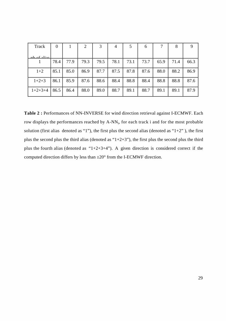
The results of Tab. 2 show that :

-the good quality of the first rank solution; the first alias (the wind direction having the

highest probability and presented in row 1 of Tab. 2) given by the NN-INVERSE matches

the I-ECMWF direction ±20° in 75% of collocations, which is a dramatic improvement

with respect to usual methods whose skill is about 60% (Rufenach, 1998, Stoffelen,

personal communication). The skill of the first and second alias (presented in row 2 of

Tab. 2) is 87%.

-the existence of a good solution among all the four aliases; about 88 % of the directions are

consistent with I-ECMWF. For the remaining 12 % we can not state the error sources

without further investigation since I-ECMWF is not an error-free reference.

These good performances are mainly due the spatial context used in the input of the S-NN and A-

NN and to the overall neural networks abilities to model non-linear phenomena.

13

5. Ambiguity removal

The problem consists in finding the best physical solution in a large combinatorial space. This

space is made of all the wind fields which are solutions with their multiple aliases. Considering

the two first aliases only and a 1000-km long swath, this space contains more than 1060 possible

wind fields. Assuming that the accuracy of the inversion is sufficiently good (i.e. it exists a

solution close to the true field in this space), then removing the ambiguities consists of finding the

most physically consistent wind field that corresponds to the true wind field. This is a very

complex problem for the following reasons:

-it is difficult to assess the physical consistency of a meteorological wind field in a

simple and fast way,

-due to the size of the combinatorial space, the search of a solution is a critical operation,

-more than one consistent field may exist; as an example two acceptable uniform wind

fields differing by 180° could be found, but only one of the two corresponds to the true

solution.

The last two points address the importance of the first rank solution (most probable wind vector)

provided by the inversion; the closer this solution to the truth, the more easily the problem is

solved. Usually the ambiguity removal algorithms (CREO, PRESCAT) solve this problem by

using a reference wind field provided by a NWP model in order to select the closest wind field in

the solution space as a start-field. Obviously, this may lead to some errors in the wind selection

14

since the prediction of NWP models could be far from the truth, particularly in locating accurately

the wind structures (front, lows, ...) over the oceans.

The ambiguity removal is performed using an adapted version of PRESCAT denoted as

PRESCAT-NN hereafter. The PRESCAT algorithm was originally developed by Stoffelen

(Stoffelen and Anderson, 1997c) and appears to be the most skillful wind ambiguity removal

procedure (Stoffelen and Anderson, 1997c) at the present time. This algorithm requires a first

guess wind field provided by a NWP model. In PRESCAT-NN, we select the different solutions

using a trade-off between the closest NN-INVERSE aliases to the direction of ECMWF model

and their probabilities given by NN-INVERSE. The resulting wind field is denoted as the start-

field. If the probability of the first alias given by NN-INVERSE is high, then priority is given to

it. If not, the chosen alias is determined by computing a normalized distance between the different

vectors provided by NN-INVERSE and the ECMWF model wind vector weighted by the

posterior probabilities of the different alias. The chosen alias corresponds to the minimum of this

distance. The resulting start-field could be very different from the ECMWF model wind field

unlike to PRESCAT. For each chosen vector of the start-field, we compute a confidence

coefficient which is a composite number taking into account the different probabilities provided

by NN-INVERSE and the different distances to ECMWF model wind direction.

Then this start field is iteratively smoothed by a 3X3 (150 km x 150 km) spatial filter which

chooses the alias in the center of the window that minimizes the global wind variance in the

spatial window. The weights of the spatial filter are initialized with the confidence coefficients

15

coming from the first step and are updated at each iteration as described in the initial Stoffelen and

Anderson (1995) method.

Fig. 7-b, 8-b and 9-b are examples of final wind fields; first NN-INVERSE has been applied on

ERS data to retrieve a set of wind solutions, then PRESCAT-NN has been applied to remove the

ambiguities among the multiple aliases. In order to evaluate the quality of the retrieved wind

fields, we have computed the one dimensional wave number spectrum for both the neural

methodology (after disambiguation) and the ECMWF wind fields (Fig. 6). It can be seen that the

neural methodology spectrum is more energetic at high wave numbers than ECMWF spectrum,

showing the ability of scatterometer winds to capture small-scale features. We can not state

firmly, without further investigation, that this increase of energy at high wave number was not

partly due to white noise colored by the non-linear processing of the neural networks.

Nevertheless, we can remark the consistency between the slope at high wave numbers and some

expected theoretical spectra (in blue lines) at these scales. Unfortunately the spatial averaging

used in the wind vector computation may filter some of small-scale structures in the wind field.

But we think it is better to increase the performance of the wind retrieval by using a spatial filter

even if we loose small scale features rather than introduce noise in the difficult attempt to keep

these small scale features.

16

6. Performances after Disambiguation and Comparisons with other Methods

We checked the performances of NN-INVERSE after the disambiguation phase and compared

them to those of ESA and CERSAT/IFREMER wind products on the S-TEST data set. This set

contains the wind vectors given by PRESCAT-NN and the dealiased wind vectors distributed by

CERSAT and by ESA. ESA wind retrieval is based on the CMOD4 GMF (Stoffelen 1995,

Stoffelen and Anderson 1997a) and CERSAT/IFREMER is based on the CMOD-IFR2 GMF

(Quilfen and Bentamy, 1994).

In these comparisons we use exactly the same data for the three methods. When one of the

methods does not provide a solution for a given signal the associated wind vectors of the two

others are also removed from the test. As a consequence S-TEST shrinks from 100000 to about

71000 comparable winds. Because this reduction is essentially due to the ESA quality control and

occasionally to the IFREMER one, the performances would be biased in favor of ESA and

IFREMER.

We also checked the accuracy of the different inversion methods independently of ambiguity

removal. For this purpose as suggested by Stoffelen and Anderson (1997b), we use a subset of S-

TEST, denoted as S90-TEST. The S90-TEST data set only contains data where the wind

direction of the three products is pointing in the same half plane as defined by the I-ECMWF

wind. If one product selects an ambiguous direction, the corresponding three products will be

thrown out from the S90-TEST database. We thus reject data with possible ambiguous direction

at 180° from S90-TEST. It would have been better to find the closest alias direction among all

17

possible directions, as done in Section 4 but this was not possible since ESA UWI product does

not provide the different wind solutions, only the dealiased one.

Tab. 3.1 (Tab. 4.1) gives the bias and the standard deviation for the wind speed error, the wind

direction error, the wind vector error and the percentage of agreement with I-ECMWF wind

direction at ±20° (denoted as Perf at @ 20° in the tables) for S-TEST (S90-TEST). The definition

of these statistical parameters is given in Appendix 1. The three first columns show the

performances computed on the true distribution of S-TEST (S90-TEST). In the three last ones

performances are computed as follows: we first considered five bins of wind speed and separately

compute the performances in each bin, later we averaged these performances in order to give the

same weight to each wind speed interval. Tab. 3.2 (Tab. 4.2) displays the distribution in % of the

data over these bins for S-TEST (S90-TEST).

Tab. 3.1 shows that the neural methodology compares well with the others methods. The

standard deviation for the wind speed and wind direction fit the ESA specifications which are

±2m/s and ±20°. In addition, we remark that the mean bin average performances of the neural

methodology are less deteriorated than others, stressing the importance of the quasi-uniform

distribution used during training. In this case, the standard deviation of wind direction and

Perf @ 20° also improve showing that at high wind speed the retrieval of wind direction is good.

Comparing Tab. 3.1 with Tab. 4.1 shows that there is a small increase in general performance but

NN-INVERSE still appears better than the two others. This is due to the accuracy of the first

rank solution of NN-INVERSE that gives considerable help to the ambiguity removal. For the

18

CERSAT product, the increase in performance is very clear. The good overall score suggests that

CMOD-IFR2 is quite an accurate GMF but that the ambiguity removal scheme is weak.

Moreover this could also be explained by the advantage of using a spatial context rather than a

one cell inversion. Whatever the accuracy of inversion and the skill of the ambiguity removal are,

it will not be possible to retrieve a good wind field if there are not sufficient well oriented winds

(first rank alias).

Fig. 7, 8 and 9 display three distinct wind fields retrieved using NN-methodology and the other

methods. We see that all the retrieved wind fields are very consistent (small divergence and no

abnormal fronts). When compared to I-ECMWF wind fields it is seen that the shape and the

center of meteorological perturbations are slightly modified showing the ability of the

scatterometer to exactly map the instantaneous wind field. In Fig. 7, the forecast low in the NE

corner is seen eastward and outside of the swath by all the inverse methods. The NWP model is

probably wrong as shown by the high consistency between the three inverse methods. In the

center of the swath we notice the only drawback due to the use of a spatial context; the gaps due

to unusable or missing ERS data increase in size because all data in G( 0) must be usable. In Fig.

8 we can note many differences between the methods. For this situation, NN-INVERSE and

PRESCAT-NN produce an outstanding wind field in comparison with the other methods. In Fig.

9 the I-ECMWF wind field is quite homogeneous and seems to be close to the measured

scatterometer winds. It results in a good agreement and a successful removal of ambiguities for all

19

inverse methods. Nevertheless, these inverted wind fields present some differences in shape and

speeds.

In order to test the consistency of the different inversion methods with respect to NWP models,

we display different scatter plots computed by using the S-TEST data set. For all of them we

also give the parameters of a linear regression of the cloud, the correlation factor and ⊥ which is

the standard deviation orthogonal to the linear regression line.

Fig. 10 a, b and c display scatterplots for the retrieved wind speed with respect to the I-

ECMWF wind field for the three methods. High winds are underestimated by all three methods.

Fig. 11 a, b and c show the scatterplots for the wind direction (after disambiguation) with respect

to I-ECMWF wind fields for the three methods.

The different statistical estimators computed from the scatter plots (linear regression, correlation

coefficient) show that the neural methodology has a good skill when compared to the two other

methods.

We also computed the scatter plots for each wind components with respect to ECMWF wind

fields (Fig. 12 a, b and c). This allows us to check the consistency of the retrieved wind vector.

One can still notice the influence of remaining wind ambiguities on the ESA and CERSAT

scatterplots appearing as abnormal scatters along the second diagonal.

20

In Fig. 13 a, b we present the histograms for the speed (a) and the direction (b) of the retrieved

winds for the three methods. These histograms are close together and to that of ECMWF showing

the good quality of the wind retrieval algorithms except for ESA at low wind speeds.

In Fig. 14 we display the histograms for the two components of the wind. It is seen that these

two-dimensional histograms are quite homogeneous and are in good agreement with this of I-

ECWMF. The large hole in the center of these histograms is due to the fact low wind speeds

(under 4 m/s) are not included in S-TEST.

In order to compare the performances of the different models, a number (the so-called Figure Of

Merit or FoM, see Appendix 2 for the definition) has been proposed by Offiler (1994). The

greater FoM, the better the inverted wind field. A FoM of 1 indicates that ESA specifications of

±2m/s and ±20° are fulfilled.

We compute FoM for the three different inverse methods on S-TEST; Tab. 5 presents the results

with respect to different I-ECMWF wind speed ranges. We also give the FoM for the true

distribution of S-TEST and the normalized one given by the mean of the FoM over each bins.

Once again neural methodology appears the most skilful model either for true distribution or for

the normalized one.

21

7-Discussion

NN-INVERSE produces a skill of 75% for rank1 ambiguity which is better than the skills of the

other methods which are around 60% (Rufenach, 1998, Stoffelen, personal communication). This

good performance is mainly due to the ability of NN-INVERSE to use a spatial context which

adds valuable information with respect to a single sigma-0 triplet. The spatial context processing

differs from a simple spatial filtering in the sense that it is intrinsically embedded in the NN-

INVERSE functioning. A tentative physical interpretation is the following: the cones

corresponding to the different cells of the spatial window are different and the position of each

sigma-0 triplet of the spatial window with respect to each cone is different in the sense that some

of them might be out of the ambiguity region contributing significantly to a correct estimation of

the first alias.

The good skill of NN-INVERSE when compared to ESA and IFREMER procedure is confirmed

on tests done using the S90-TEST database.

The PRESCAT NN takes into account the posterior probabilities on the wind direction given by

NN-INVERSE to remove the ambiguities. The good performance of the NN retrieved wind are

thus due to the combination of NN-INVERSE and PRESCAT-NN. As in every methodological

comparison, bias may be introduced due to the fact that the CMOD4 GMF (ESA GMF) and

CMOD2-I3 (IFREMER GMF) used for the inversion, have been calibrated using ECMWF

output during 1992-1993. Since this period, the quality of ECMWF winds has dramatically

22

improved leading to a bias in the comparison with the NN method which has been trained using

data from July 1994 to April 1996.

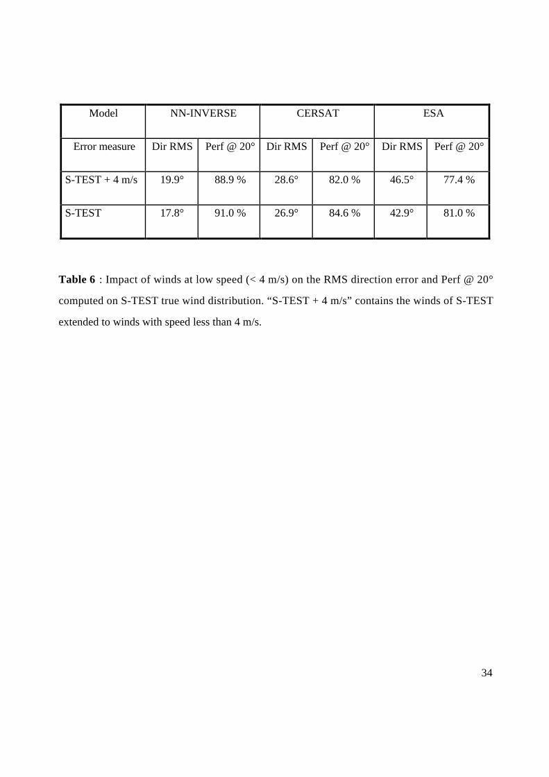
All three methods yield poor performance when retrieving the wind direction at low wind speed.

Tab. 6 compares the statistics on wind direction computed for S-TEST true distribution with S-

TEST true distribution extended to wind with speed less than 4 m/s. Although such winds

represent only 6.5 % of the data, their impact on wind direction RMS error and thus Perf @ 20°

is significantly obvious. The three methods increase their RMS error on wind direction by 2.1°

for NN-INVERSE, 1.7° for CERSAT and 3.6° for ESA. They decrease Perf @ 20° by 2.1 %, 2.6

% and 3.6 % respectively. Since all methods show this deficiency it seems that this phenomenon

is due to an intrinsic limitation of the physics of the scatterometer rather than to a modelling

deficiency. We suggest that the development of the surface ripple waves under low wind is not

sufficient to ensure an accurate estimation of wind direction. For this reason, we recommend very

careful use of scatterometer winds when their speed is less than 4 m/s.

Obviously the use of a spatial context gives directional information that explains the good skill of

the first rank solution and consequently the high quality of the final wind fields after ambiguity

removal. The main drawback is that all 13x3 sigma-0 must be used in the input; the area

containing unusable ERS measurements increase in size in comparison with the one-cell inversion.

This impact can be seen in the middle swath of Fig. 7-b. Such a spatial context could also

introduce a possible spatial filtering on the wind field. Besides since we used a NWP to train the

23

relationships between the wind and ERS signal, it may result a loss of geophysical variance at the

lowest spatial scales.

8-Conclusion

This paper presents a neural networks methodology to retrieve the wind vector from ERS1

scatterometer data. The inversion of the scatterometer data is complex since the sigma-0 triplets

can lay in regions of the sigma-0 space where the direction is intrinsically ambiguous as explained

in the introduction. NN-INVERSE provides an estimate of the posterior probability of the

different alias for the wind direction. The most probable wind direction (rank 1 solution) given by

NN-INVERSE has a skill of 75% while those of the other methods is of about 60%. This clearly

shows the improvement of NN-INVERSE with respect to the other methods. The remaining

ambiguities are then removed by an adapted version of the PRESCAT algorithm which uses a

meteorological wind field provided by a NWP model as a first guess. The probability estimation

of the neural network wind directions is explicitly introduced as a constraint in the adapted

version of PRESCAT. After disambiguation, the correct direction is retrieved 89% of the time.

Due to the high skill of the first alias provided by NN-INVERSE model, we can envisage a self-

consistent neural network ambiguity removal method similar to this proposed in Badran et al

(1991). These authors showed that with 25% of ambiguous wind direction, 99 % of them were

corrected with the NN approach. Thanks to the good performances displayed in Tab. 2 for the

direction, we can thus envisage to remove the ambiguity without any external information.

24

Systematic comparisons with other methods have been processed. It appears that the NN has a

very good skill. The advantages of the neural network method are linked to:

- their ability of modeling non-linear phenomena that do not assume the forms of the functions

and noises involved in the physical processes,

- the ability to use a spatial context which improves greatly the performance of the first alias

solution and thus the skill of any ambiguity removal algorithm.

- the ability to directly estimate the posterior probability of the different wind aliases with

neural networks working in classifier mode. Those probabilities enhance the skill of the

disambiguation phase.

Owing to its good performances the neural networks methodology is an efficient alternative for

scatterometer wind field retrieval. The fact that NN-INVERSE only does algebraic operations is a

major advantage for operational use.

Acknowledgements

We would like to thank the CERSAT/IFREMER who provided the collocations between ERS1

sigma-0 and the analyzed wind vectors of the ECMWF Model. We also thank D. Cornford for

stimulating and enlightening discussions. The present study was supported by the EC program

NEUROSAT (ENV4-CT96-0314).

25

References

Badran, F., S. Thiria, and M. Crepon: Wind ambiguity removal by the use of neural network techniques. J.

Geophys. Res., 96, 20521-20529, 1991.

Bishop, C. M.: Neural Networks for pattern recognition, Oxford University Press, 482 p., 1995.

Cavanié, A., and D. Offiler : ERS1 Wind Scatterometer: Wind Extraction and Ambiguity Removal. Proc. of

IGARSS 86 Symposium, Zurich, ( ESA SP-254), 1986.

Mejia, C., S. Thiria, F. Badran, and M. Crépon, A Neural Network Approach for Wind Retrieval from the ERS-1

Scatterometer Data, IEEE Ocean94 Proc., Brest-Sept. 13-16 (1), 1994.

Offiler D. : The Calibration of ERS1 Satellite scatterometer winds. J. Atm. Ocean Tech.., 1002-1017, 1994

Quilfen, Y. and A. Bentamy : Calibration/Validation of ERS-1 scatterometer precision, Proc. of IGARSS 94,

Pasadena, United States, 945-947, 1994.

Richard, M. D. and R. P. Lippman : Neural Network Classifiers Estimate Bayesian a posteriori Probabilities,

Neural Computation, 3, 461-483, 1991

Rufenach, C. : Comparison of Four ERS-1 Scatterometer Wind retrieval Algorithms with buoys measurements. J.

Atm. Ocean Tech.., 304-313, 1998.

Stoffelen, A and D. Anderson :The ECMWF Contribution to the Characterization, Interpretation, Calibration and

Validation of ERS-1 Scatterometer Backscatter Measurements, and Winds, and their use in Numerical

Weather Prediction Models , ESA Contract Reports, 1995.

Stoffelen, A and D. Anderson : Scatterometer data interpretation: Measurement Space and Inversion. J. Atm. Ocean

Tech.., 1298-1313, 1997a.

Stoffelen, A and D. Anderson : Scatterometer data interpretation: Estimation and validation of the transfer function

CMOD4. J. Geophys. Res. 102, 5767-5780, 1997b.

Stoffelen, A and D. Anderson : Ambiguity removal and assimilation of scatterometer. Q. J. Roy. Meteorol. Soc.

123, 491-518, 1997c

Thiria, S., F. Badran, C. Mejia and M. Crepon : A Neural Network Approach for modelling Non Linear Transfer

functions : Application for Wind Retrieval from Spaceborne Scatterometer Data. J. Geophys. Res. 98, 22827-

22841, 1993.

26

APPENDIX 1

The bias, standard deviation an RMS are defined as:

BIAIS =

val ic − val i

M( )i

∑

N BIAIS =

val ic − val i

M( )i

∑

N RMS =

valic − vali

M( )2

∑N

where val est represents an estimate, val ref the true value, and N is number of data..

Lest us define resj as res val valj jest

jref= − .

For wind vectors the residual and the bias are also vectors and their algebraic values are given by a

norm in R2.

For wind direction

if then

if then

else

val val res val val

val val res val val

res val val

jest

jref

i jest

jref

jest

jref

i jest

jref

i jest

jref

− < − = − +

− > = − −

= −

180 360

180 360

The Perf@20° performances is the percentage of agreement between the estimated wind direction

and the reference wind direction : Perf @20° = 100Cardinal res j < 20°{ }

N, with the same

definition as for the residuals of wind direction.

27

APPENDIX 2

Figure of Merit (FoM)

This non-dimensional number has been proposed by D Offiler (1994) for evaluating the

performances of the scatterometer retrieved winds. It is of the form:

FoM =F1 + F2 + F3

3

with

F1 =40

vbias +10v stdv + bias + stdv

; F2 =1

2

2

vrms

+20

rms

; F3 =

4

Vrms

Where v is the wind speed, is the wind azimuth and r

V the wind vector.

These numbers are computed with the residuals defined in Appendix 1 except for wind vector

RMS Vrms which is defined with the following residual:

Vres = Vd2 + Vecmwf

2 − 2 Vd2Vecmwf

2 cos( res ) .

Assuming bias free estimators, FoM = 1 if specifications of ±2m/s in wind speed error and ±20°

in wind direction error are exactly fulfilled. The greater FoM, the better the inverse wind field.

28

Tables

track 0 1 2 3 4 5 6 7 8 9

bias (m/s) -0.2 0.0 -0.1 -0.1 -0.1 -0.1 -0.1 -0.1 0.0 0.0

RMS (m/s) 1.6 1.6 1.5 1.6 1.6 1.6 1.6 1.6 1.6 1.7

Table 1 : Performances of NN-INVERSE when approximating the wind speed : the first row

gives the bias with respect to the track and the second gives the RMS.

29

Track

nb of alias

0 1 2 3 4 5 6 7 8 9

1 78.4 77.9 79.3 79.5 78.1 73.1 73.7 65.9 71.4 66.3

1+2 85.1 85.0 86.9 87.7 87.5 87.8 87.6 88.0 88.2 86.9

1+2+3 86.1 85.9 87.6 88.6 88.4 88.8 88.4 88.8 88.8 87.6

1+2+3+4 86.5 86.4 88.0 89.0 88.7 89.1 88.7 89.1 89.1 87.9

Table 2 : Performances of NN-INVERSE for wind direction retrieval against I-ECMWF. Each

row displays the performances reached by A-NNi, for each track i and for the most probable

solution (first alias denoted as “1”), the first plus the second alias (denoted as “1+2” ), the first

plus the second plus the third alias (denoted as “1+2+3”), the first plus the second plus the third

plus the fourth alias (denoted as “1+2+3+4”). A given direction is considered correct if the

computed direction differs by less than ±20° from the I-ECMWF direction.

30

Data Set

71436 data

S-TEST

True Distribution

S-TEST

Mean Bin Average

inverse model NN-INVERSE CERSAT ESA NN-INVERSE CERSAT ESA

Speed Bias

in m/s

0.2 -0.1 -0.8 -0.5 -1.26 -2.1

Speed Stdv

in m/s

1.4 1.5 1.5 1.7 1.6 1.6

Dir Bias

in degree

-0.2 -0.0 -0.4 -0.1 -0.5 1.0

Dir Stdv

in degree

17.8 26.9 42.9 16.3 21.5 43.7

Vector Bias

in m/s

0.2 0.4 0.5 0.8 1.4 2.1

Vector Stdv

in m/s

2.8 3.6 5.1 3.6 4.1 7.2

Perf @ 20°

in %

91.1 84.6 81.0 92.3 88.1 83.6

Table 3.1 : Performances of the different inversion methods on S-TEST ; in italic bold

performances when they are equivalent (difference between the performances less than 5%), in

bold the best performances (difference between the performances between 5% and 10%), in bold

and underlined the performances which are the highest (higher than 10 %).

31

I-ECMWF

speed in m/s

< 4 4 - 8 8 - 12 12 - 16 16 - 20 > 20

% of S-TEST 6.46 51.79 29.84 9.37 2.08 0.47

Table 3.2 : distribution in % of the data used in Tab. 3.1 on the bins. The shaded column is only

given for information, those winds (speed less than 4 m/s) are not used in statistics.

32

Data Set

69133 data

S90-TEST

True Distribution

S90-TEST

Mean Bin Average

inverse model NN-INVERSE CERSAT ESA NN-INVERSE CERSAT ESA

Speed Bias

in m/s

0.1 -0.1 -0.8 -0.7 -1.3 -2.1

Speed Stdv

in m/s

1.3 1.4 1.5 1.6 1.5 1.6

Dir Bias

in degree

-0.7 -0.9 -0.6 -0.3 -1.2 0.8

Dir Stdv

in degree

12.9 15.2 40.0 12.1 13.4 42.2

Vector Bias

in m/s

0.2 0.3 0.5 0.8 1.3 2.1

Vector Stdv

in m/s

2.3 2.6 4.8 3.1 3.3 7.0

Perf @ 20°

in %

91.4 86.6 82.2 92.6 89.4 84.3

Table 4.1 : Performances of the different inversion methods on S90-TEST ; in italic bold

performances when they are equivalent (difference between the performances less than 5%), in

bold the best performances (difference between the performances between 5% and 10%), in bold

and underlined the performances which are the highest (higher than 10 %).

33

I-ECMWF

speed in m/s

< 4 4 - 8 8 - 12 12 - 16 16 - 20 > 20

% of S90-TEST 6.00 51.83 30.14 9.41 2.13 0.49

Table 4.2 : distribution in % of the data used in Tab. 4.1 on the bins. The shaded column is only

given for information, those winds (speed less than 4 m/s) are not used in statistics.

speed m/s true <4 4 - 8 8 - 12 12 - 16 16 - 20 >20 mean

NN-INVERSE 1.29 1.15 1.55 1.23 1.04 1.00 1.03 1.17

CERSAT 1.05 1.05 1.23 1.05 0.81 1.00 1.01 1.02

ESA 0.76 0.88 1.01 0.72 0.58 0.54 0.43 0.67

Table 5 : FoM for S-SET with respect to the wind speed and for the true distribution of S-TEST

and averaged over each bins. The shaded column gives the FoM for winds speed less than 4 m/s

and is given only for information, those winds are not used for computing the FoM for true

distribution and bin average.

34

Model NN-INVERSE CERSAT ESA

Error measure Dir RMS Perf @ 20° Dir RMS Perf @ 20° Dir RMS Perf @ 20°

S-TEST + 4 m/s 19.9° 88.9 % 28.6° 82.0 % 46.5° 77.4 %

S-TEST 17.8° 91.0 % 26.9° 84.6 % 42.9° 81.0 %

Table 6 : Impact of winds at low speed (< 4 m/s) on the RMS direction error and Perf @ 20°

computed on S-TEST true wind distribution. “S-TEST + 4 m/s” contains the winds of S-TEST

extended to winds with speed less than 4 m/s.