Neural Nets and Symbolic Reasoning Hopfield Networks

2

Outline

The idea of pattern completion

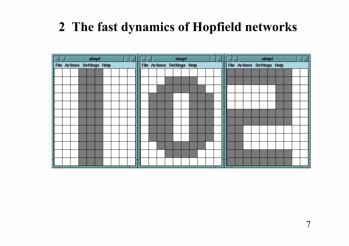
The fast dynamics of Hopfield networks

Learning with Hopfield networks

Emerging properties of Hopfield networks

Conclusions

3

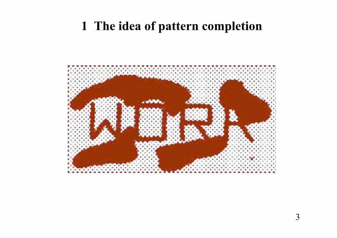
1 The idea of pattern completion

4

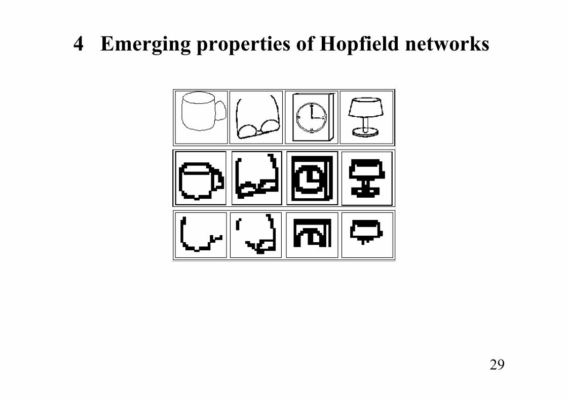
Example from visual recognition

• Noisy or underspecified input

• Mechanism of pattern completion (using stored images)

• Stored patterns are addressable by content, not pointers (as in traditional computer memories)

5

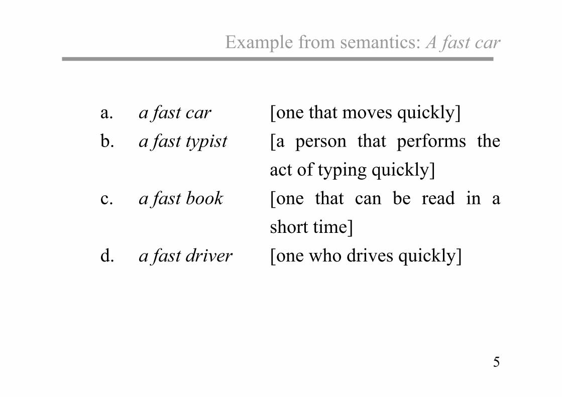
Example from semantics: A fast car

a. a fast car [one that moves quickly]

b. a fast typist [a person that performs the act of typing quickly]

c. a fast book [one that can be read in a short time]

d. a fast driver [one who drives quickly]

6

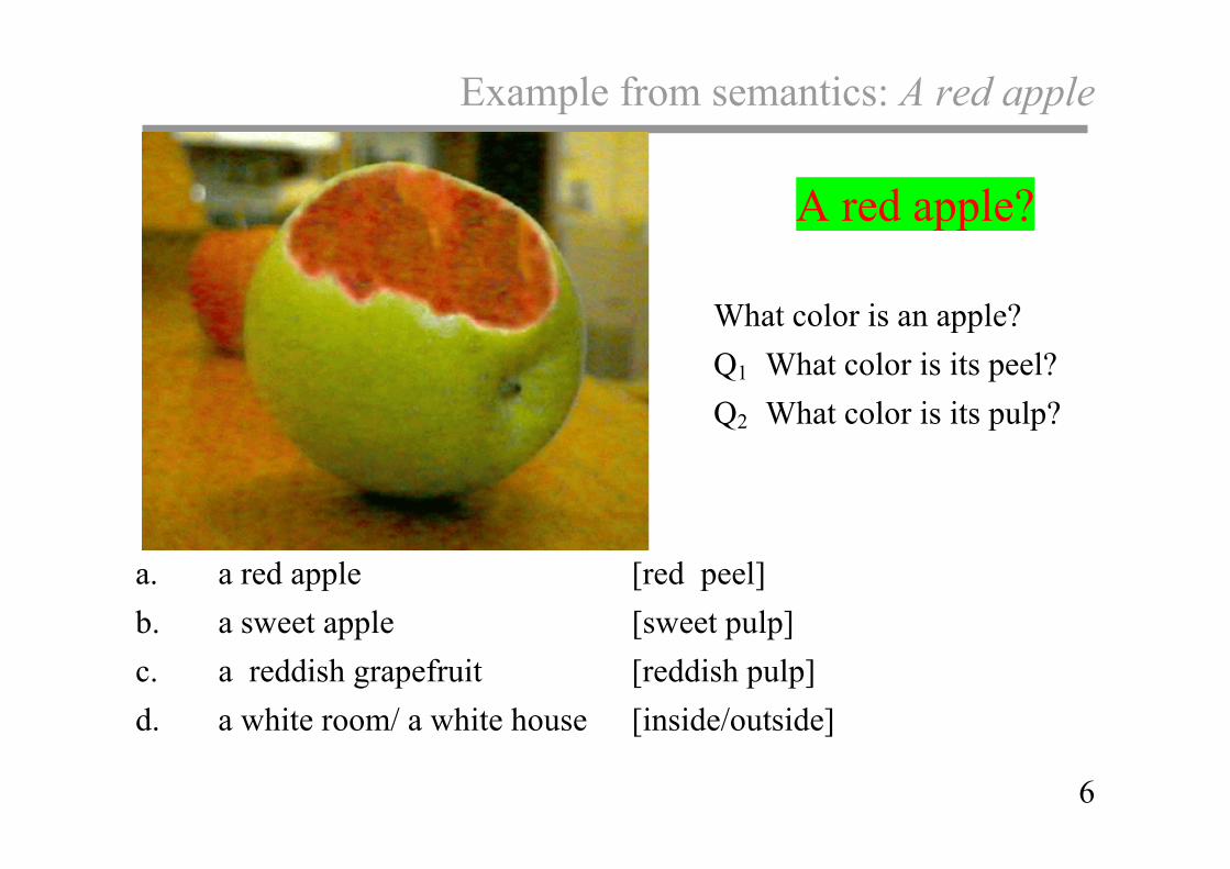
Example from semantics: A red apple A red apple?

What color is an apple? Q1 What color is its peel? Q2 What color is its pulp?

a. a red apple [red peel] b. a sweet apple [sweet pulp] c. a reddish grapefruit [reddish pulp] d. a white room/ a white house [inside/outside]

7

2 The fast dynamics of Hopfield networks

8

Abstract description of neural networks

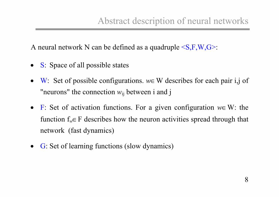
A neural network N can be defined as a quadruple <S,F,W,G>:

• S: Space of all possible states

• W: Set of possible configurations. w∈W describes for each pair i,j of "neurons" the connection wij between i and j

• F: Set of activation functions. For a given configuration w∈W: the function fw∈F describes how the neuron activities spread through that network (fast dynamics)

• G: Set of learning functions (slow dynamics)

9

Dynamic systems

Discrete dynamic systems

))(()1( tsgts rr=+ s(t) is a vector of the space of states S

Continuous dynamic systems

))(()( tsgtsdtd rr

= the function g describes the fast dynamics

Dynamical Systems + Neural Networks =Neurodynamics • Tools from dynamical systems, statistics and statistical physics can be

used. Very rich field. • The triple <S,F,W> corresponds to the fast neurodynamics

10

The importance of recurrent systems

What can recurrent networks do?

• Associative memories

• Pattern completion

• Noise removal

• General networks (can implement everything feedforward networks

can do, and even emulate Turing machines)

• Spatio-temporal pattern recognition

• Dynamic reconstruction

11

Hopfield networks

J.J.Hopfield (1982), "Neural networks and physical systems with emergent collective computational abilities", Proceedings of the National Academy of Sciences 79, 2554-2558.

An autoassociative, fully connected network with binary neurons, asynchronous updates and a Hebbian learning rule. The “classic” recurrent network

Computational properties of use to biological organisms or to the construction of computers can emerge as collective properties of systems having a large number of simple equivalent components (or neurons). The physical meaning of content-addressable memory is described by an appropriate phase space flow of the state of the system. …

12

Concise description of the fast dynamics Let the interval [-1,+1] be the working range of each neuron

+1: maximal firing rate 0: resting -1 : minimal firing rate)

S = [-1, 1] n

wij = wji , wii = 0

ASYNCHRONOUS UPDATING: θ (Σj wij⋅sj(t)), if i = rand(1,n) s i(t+1) = si(t), otherwise

Step 3 Step 4

Step 98651 Step 98652

Step 1 Step 2

13

Definition of resonances of a dynamical system

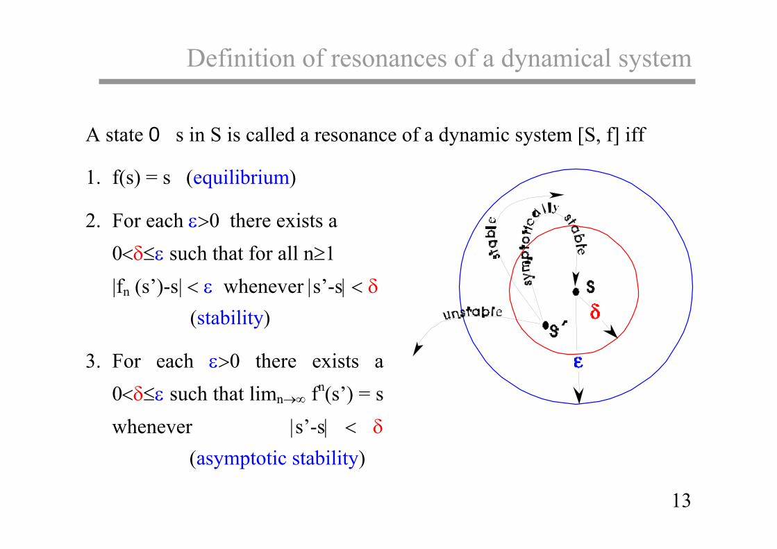
A state 0 s in S is called a resonance of a dynamic system [S, f] iff

1. f(s) = s (equilibrium)

2. For each ε>0 there exists a 0<δ≤ε such that for all n≥1 |fn (s’)-s| < ε whenever |s’-s| < δ

(stability)

3. For each ε>0 there exists a 0<δ≤ε such that limn→∞ fn(s’) = s whenever |s’-s| < δ (asymptotic stability)

14

Energy and convergence

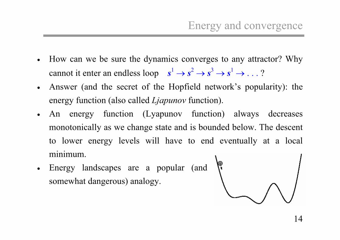
• How can we be sure the dynamics converges to any attractor? Why

cannot it enter an endless loop s1 → s2 → s3 → s1 → . . . ?

• Answer (and the secret of the Hopfield network’s popularity): the energy function (also called Ljapunov function).

• An energy function (Lyapunov function) always decreases monotonically as we change state and is bounded below. The descent to lower energy levels will have to end eventually at a local minimum.

• Energy landscapes are a popular (and somewhat dangerous) analogy.

15

Resonance systems

Definition A neural network [S,W,F] is called a resonance system iff limn→∞ fn(s) exists and is a resonance for each s∈S and f∈F.

Theorem 1 (Cohen & Großberg 1983) Hopfield networks are resonance systems. (The same holds for a large class of other systems: The McCulloch-Pitts model (1943), Cohen-Grossberg models (1983), Rumelhart's Interactive Activation model (1986), Smolensky's Harmony networks (1986), etc.)

16

Ljapunov-function

Lemma (Hopfield 1982) The function E(s) = -½ ∑i,j wij si sj is a Ljapunov-function of the system in the case of asynchronous updates. That means: • when the activation state of the network changes, E can either

decrease or remain the same. Consequence: The output states limn→∞ fn(s) can be characterized as the local minima of the Ljapunov-function. Remark: E(s) = -½ ∑i,j wij si sj = -∑i<j wij si sj (symmetry!)

17

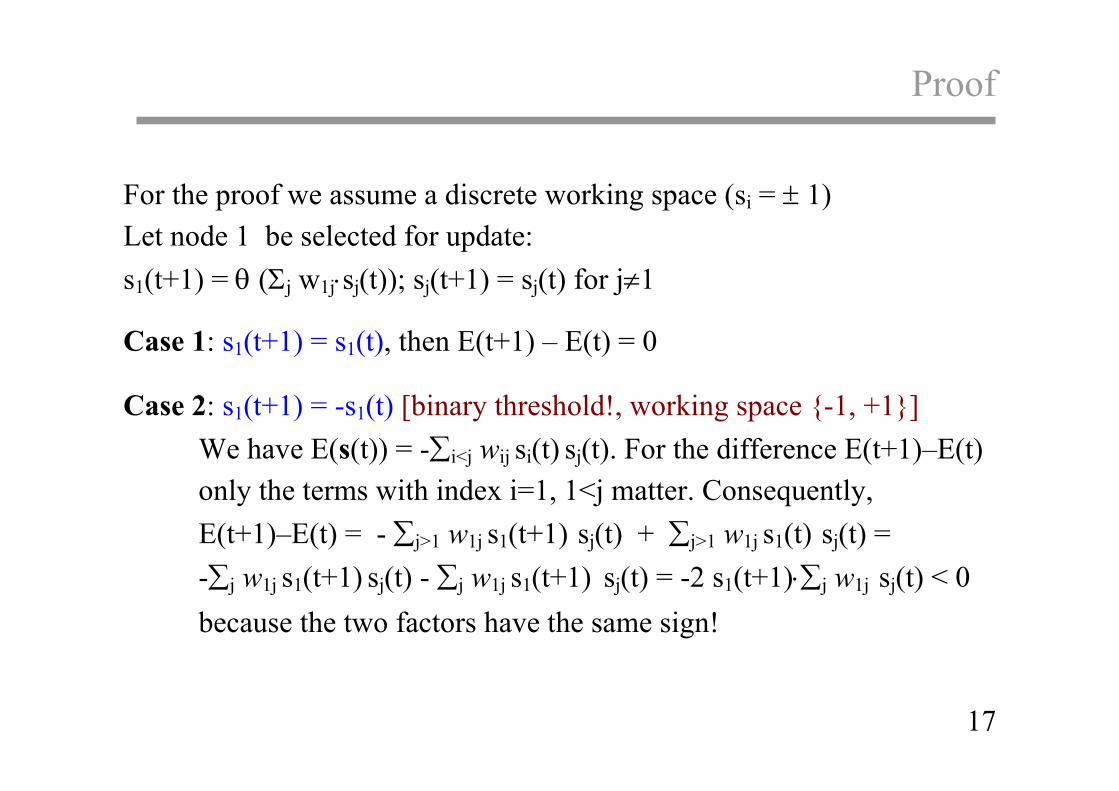
Proof

For the proof we assume a discrete working space (si = ± 1) Let node 1 be selected for update: s1(t+1) = θ (Σj w1j⋅sj(t)); sj(t+1) = sj(t) for j≠1

Case 1: s1(t+1) = s1(t), then E(t+1) – E(t) = 0

Case 2: s1(t+1) = -s1(t) [binary threshold!, working space {-1, +1}] We have E(s(t)) = -∑i<j wij si(t) sj(t). For the difference E(t+1)–E(t) only the terms with index i=1, 1<j matter. Consequently,

E(t+1)–E(t) = - ∑j>1 w1j s1(t+1) sj(t) + ∑j>1 w1j s1(t) sj(t) = -∑j w1j s1(t+1) sj(t) - ∑j w1j s1(t+1) sj(t) = -2 s1(t+1)⋅∑j w1j sj(t) < 0 because the two factors have the same sign!

18

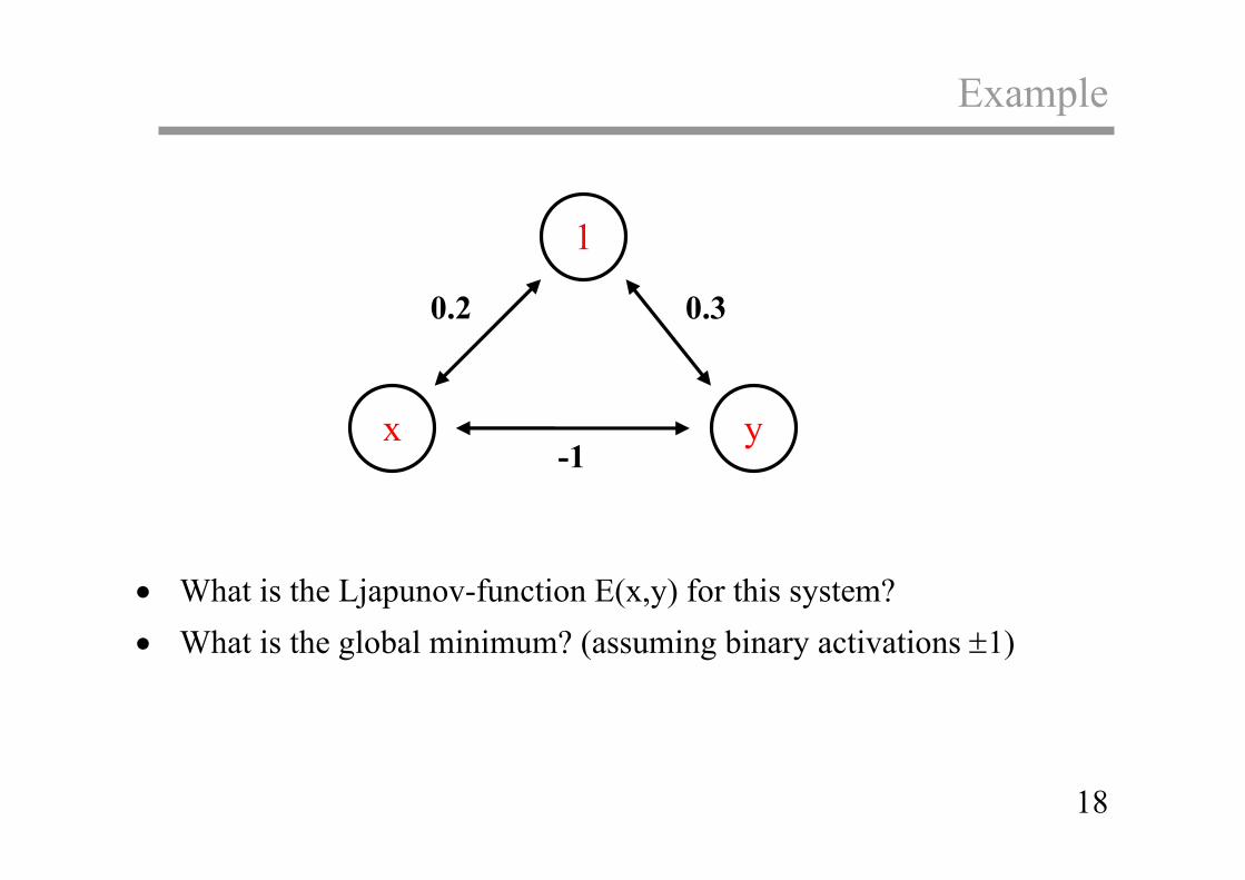
Example

• What is the Ljapunov-function E(x,y) for this system? • What is the global minimum? (assuming binary activations ±1)

0.3

-1

0.2

1

x y

19

Example

E = -∑i<j wij si sj E(x,y) = –0.2x – 0.3y + xy

x y E 1 1 -1 -1

1 -1 1 -1

.5 -.9 -1.1 1.5

0.3

-1

0.2

1

x y

20

Global Minima

Theorem 2 (Hopfield 1982) The output states limn→∞ fn(s) can be characterized as the global minima of the Ljapunov-function if certain stochastic update functions f are considered ("simulated annealing").

What we need is a probability distribution for the states P(s) for each time and a stochastic update rule which respects that there is some stochastic disturbance during updating the activation vectors.

E start

A

Basynchronousupdates

asynchronous updates with fault

21

Simulated annealing

How to escape local minima?

• One idea: add randomness, so that we can go uphill sometimes. Then we can escape shallow local minima and more likely end up in deep minima. We can use a probabilistic update rule.

• Too little randomness: we end up in local minima. Too much, and we jump around instead of converging.

• Solution by analogy from thermodynamics: annealing through slow cooling. Start the network in a high temperature state, and slowly decrease the temperature according to an annealing schedule.

22

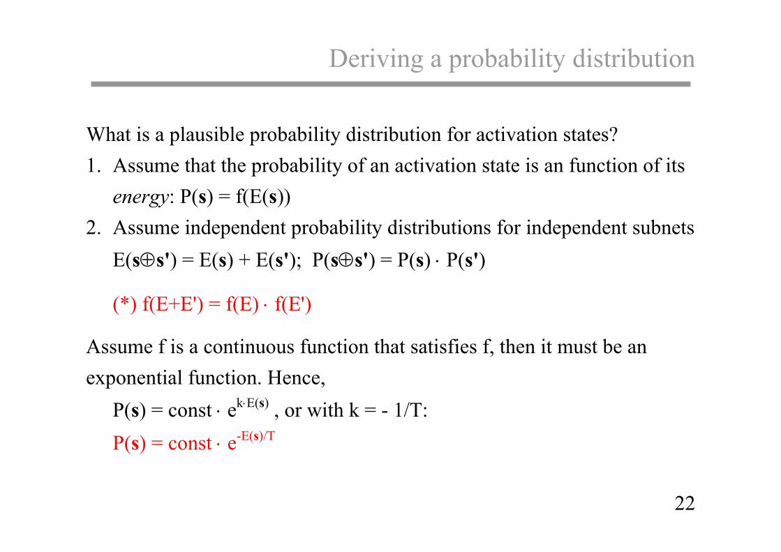
Deriving a probability distribution

What is a plausible probability distribution for activation states? 1. Assume that the probability of an activation state is an function of its

energy: P(s) = f(E(s)) 2. Assume independent probability distributions for independent subnets

E(s⊕s') = E(s) + E(s'); P(s⊕s') = P(s) ⋅ P(s')

(*) f(E+E') = f(E) ⋅ f(E')

Assume f is a continuous function that satisfies f, then it must be an exponential function. Hence,

P(s) = const ⋅ ek⋅E(s) , or with k = - 1/T: P(s) = const ⋅ e-E(s)/T

23

A probabilistic update rule

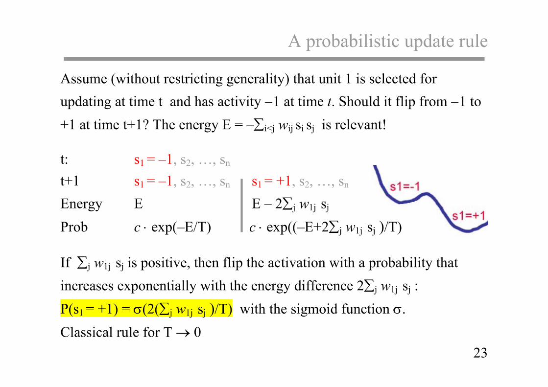
Assume (without restricting generality) that unit 1 is selected for updating at time t and has activity −1 at time t. Should it flip from −1 to +1 at time t+1? The energy E = –∑i<j wij si sj is relevant!

t: s1 = –1, s2, …, sn t+1 s1 = –1, s2, …, sn s1 = +1, s2, …, sn Energy E E – 2∑j w1j sj Prob c ⋅ exp(–E/T) c ⋅ exp((–E+2∑j w1j sj )/T)

If ∑j w1j sj is positive, then flip the activation with a probability that increases exponentially with the energy difference 2∑j w1j sj : P(s1 = +1) = σ(2(∑j w1j sj )/T) with the sigmoid function σ. Classical rule for T → 0

24

The Metropolis algorithm

At each step, select a unit and calculate the energy difference ∆E between its current state and its flipped state.

If ∆E ≥ 0 don't flip the unit. If ∆E < 0, flip the unit with probability σ(-∆E/T).

After around n such steps, lower the temperature further and repeat the cycle again. Geman and Geman (1984) If the temperature in cycle k satisfies for every k and T0 is large enough, then the system will with probability one converge to the minimum energy configuration.

25

3 Learning with Hopfield networks

26

The basic idea

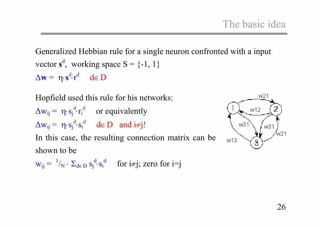
Generalized Hebbian rule for a single neuron confronted with a input vector sd, working space S = {-1, 1} ∆w = η⋅sd⋅rd d∈D

Hopfield used this rule for his networks: ∆wij = η⋅sj

d⋅rid or equivalently

∆wij = η⋅sjd⋅si

d d∈D and i≠j!

In this case, the resulting connection matrix can be shown to be wij = 1/N ⋅ Σd∈D sj

d⋅sid for i≠j; zero for i=j

27

Example

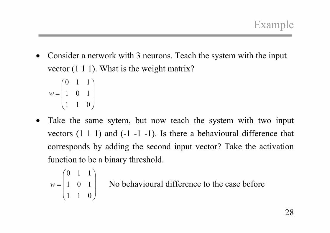
• Consider a network with 3 neurons. Teach the system with the input vector (1 1 1). What is the weight matrix?

• Take the same system, but now teach the system with two input

vectors (1 1 1) and (-1 -1 -1). Is there a behavioural difference that corresponds by adding the second input vector? Take the activation function to be a binary threshold.

28

Example

• Consider a network with 3 neurons. Teach the system with the input vector (1 1 1). What is the weight matrix?

=

011101110

w

• Take the same sytem, but now teach the system with two input vectors (1 1 1) and (-1 -1 -1). Is there a behavioural difference that corresponds by adding the second input vector? Take the activation function to be a binary threshold.

=

011101110

w No behavioural difference to the case before

29

4 Emerging properties of Hopfield networks

30

Auto-associative memory

Store a set of patterns { sd } in such a way that when presented with a pattern sx it will respond with the stored pattern that is most similar to it. Maps patterns to patterns of the same type. (e.g. a noisy or incomplete record maps to a clear record).

• Mechanism of pattern completion: The stored patterns are attractors. If the system starts outside any of the attractors it will begin to move towards one of them.

• Stored patterns are addressable by content, not pointers (as in traditional computer memories)

See the link Hopfield network as associative memory on the website

31

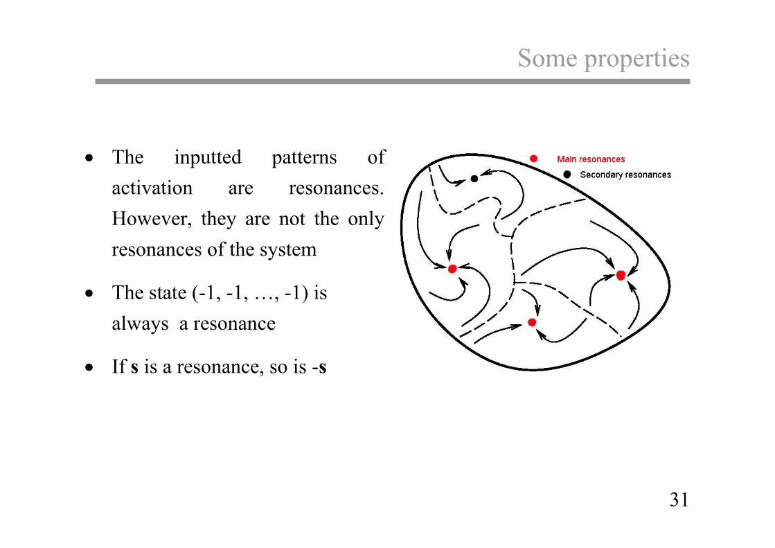
Some properties • The inputted patterns of

activation are resonances. However, they are not the only resonances of the system

• The state (-1, -1, …, -1) is always a resonance

• If s is a resonance, so is -s

32

Capacity

• How many patterns can a n unit network store? • The more patterns added, the more crosstalk and spurious states

(second. resonances). The larger the network, the greater the capacity. • It turns out that the capacity is

roughly proportional to n: M = α ⋅ n, where M is the number of inputted pattern that can be correctly reproduced (with an error probability of p)

33

Phase transition

• If we want perror = 0.01, then M = 0.105 ⋅ n. This is an upper bound.

• At M = 0.138⋅ n patterns the network suddenly breaks down and cannot recall anything useful (“catastrophic forgetting”).

• The behaviour around α = 0.138 corresponds to a phase transition in physics (solid – liquid).

• Physical analogy: spin glasses. Unit states correspond to spin states in a solid. Each spin is affected by the spins of the others plus thermal noise, and can flip between two states (1 and -1).

34

5 Conclusions

Hopfield nets are "the harmonic oscillator" in modern neurodynamics

the idea of resonance systems

the idea of simulated annealing

the idea of content addressable memory

very simple learning theory based on the generalized Hebbian rule.