neural importance sampling - tom94.net · neural importance sampling thomas mÜller, disney...

Neural Importance Sampling

THOMAS MÜLLER, Disney Research & ETH Zürich

BRIAN MCWILLIAMS, Disney Research

FABRICE ROUSSELLE, Disney Research

MARKUS GROSS, Disney Research & ETH Zürich

JAN NOVÁK, Disney Research

We propose to use deep neural networks for generating samples in Monte

Carlo integration. Our work is based on non-linear independent compo-

nents estimation (NICE), which we extend in numerous ways to improve

performance and enable its application to integration problems. First, we

introduce piecewise-polynomial coupling transforms that greatly increase

the modeling power of individual coupling layers. Second, we propose to

preprocess the inputs of neural networks using one-blob encoding, which

stimulates localization of computation and improves inference. Third, we de-

rive a gradient-descent-based optimization for the KL and the χ 2divergence

for the specific application of Monte Carlo integration with unnormalized

stochastic estimates of the target distribution. Our approach enables fast and

accurate inference and efficient sample generation independently of the di-

mensionality of the integration domain. We show its benefits on generating

natural images and in two applications to light-transport simulation: first,

we demonstrate learning of joint path-sampling densities in the primary

sample space and importance sampling of multi-dimensional path prefixes

thereof. Second, we use our technique to extract conditional directional

densities driven by the triple product of the rendering equation and leverage

them for path guiding. In all applications, our approach yields on-par or

higher performance than competing techniques at equal sample count.

CCS Concepts: • Computing methodologies → Neural networks; Raytracing; Supervised learning by regression; Reinforcement learning; • Mathe-matics of computing→ Sequential Monte Carlo methods;

1 INTRODUCTION

Solving integrals is a fundamental problem of calculus that appears

in many disciplines of science and engineering. Since closed-form

antiderivatives exist only for elementary problems, many applica-

tions resort to numerical recipes. Monte Carlo (MC) integration is

one such approach, which relies on sampling a number of points

within the integration domain and averaging the integrand thereof.

The main drawback of MC methods is the relatively low conver-

gence rate. Many techniques have thus been developed to reduce

the integration error, e.g. via importance sampling, control variates,

Authors’ addresses: Thomas Müller, Disney Research & ETH Zürich, muelltho@

inf.ethz.ch; Brian McWilliams, Disney Research, [email protected]; Fabrice

Rousselle, Disney Research, [email protected]; Markus Gross,

Disney Research & ETH Zürich, [email protected]; Jan Novák, Disney Research,

[email protected].

© 2018 Copyright held by the owner/author(s).

Markov chains, integration on multiple accuracy levels, and use of

quasi-random numbers.

In this work, we focus on the concept of importance sampling and

propose to parameterize the sampling density using a collection of

neural networks. Generative neural networks have been successfully

leveraged in many fields, including signal processing, variational

inference, and probabilistic modeling, but their application to Monte

Carlo integration—in the form of sampling densities—remains to be

investigated; this is what we strive for in the present paper.

Given an integral

F =

∫D

f (x) dx , (1)

we can introduce a probability density function (PDF) q(x), which,under certain constraints, allows expressing F as the expected ratio

of the integrand and the PDF:

F =

∫D

f (x)

q(x)q(x) d(x) = E

[f (X )

q(X )

]. (2)

The above expectation can be approximated using N independent,

randomly chosen points X1,X2, · · ·XN ;Xi ∈ D,Xi ∼ q(x), withthe following MC estimator:

F ≈ ⟨F ⟩N =1

N

N∑i=1

f (Xi )

q(Xi ). (3)

The variance of the estimator, besides being inversely proportional

to N , heavily depends on the shape of q. If q follows normalized fclosely, the variance is low. If the shapes of the two differ signifi-

cantly, the variance tends to be high. In the special case when sam-

ples are drawn from a PDF proportional to f (x), i.e. p(x) ≡ f (x)/F ,we obtain a zero-variance estimator, ⟨F ⟩N = F , for any N ≥ 1.

It is thus crucial to use expressive sampling densities that match

the shape of the integrand well. Additionally, generating sample Ximust be fast (relative to the cost of evaluating f ), and invertible. Thatis, given a sample Xi , we require an efficient and exact evaluation

of its corresponding density q(Xi )—a necessity for evaluating the

unbiased estimator of Equation (3). Being expressive, fast to evaluate,

and invertible are the key properties of good sampling densities,

and all our design decisions can be traced back to these.

We focus on the general setting where little to no prior knowledge

about f is given, but f can be observed at a sufficiently high number

of points. Our goal is to extract the sampling density from these

observations while handling complex distributions with possibly

many modes and arbitrary frequencies. To that end, we employ

variational inference to approximate the ground-truth p(x) using agenerative probabilistic parametric model q(x ;θ ) that utilizes deepneural networks.

39:2 • Müller et al.

Our work builds on approaches that are capable of compactly

representing complex manifolds in high-dimensional spaces, and

permit fast and exact inference, sampling, and density estimation.

We extend the work of Dinh et al. [2014, 2016] on learning stably

invertible transformations, represented by so-called coupling layers,that are stacked to produce highly nonlinear mappings between

an observation x and a latent variable z. Specifically, we presentpiecewise-polynomial coupling layers that greatly increase the ex-

pressive power of individual coupling layers, allowing us to employ

fewer of those and thereby reduce the total cost of evaluation.

After reviewing related work on variational inference and gener-

ative modeling in Section 2, we detail the framework of non-linearindependent components estimation (NICE) [Dinh et al. 2014, 2016] in

Section 3, which forms the foundation of our approach. In Section 4,

we describe a class of invertible piecewise-polynomial coupling trans-forms that replace affine transforms proposed in the original work,

and one-blob-encoded network inputs, which stimulate localization

of computation and improve inference. We illustrate the benefits

on a few low-dimensional density-estimation problems and test the

performance when learning the (high-dimensional) distribution of

natural images. In Section 5, we apply NICE to Monte Carlo integra-

tion and propose an optimization strategy for minimizing estimation

variance. Finally, we apply the proposed approach to light-transport

problems in Section 6: we use NICE with our polynomial warps to

guide the construction of light paths and demonstrate that, while

currently being impractical due to large computational overhead,

it outperforms the state of the art at equal sample count in path

guiding and primary-sample-space path sampling.

2 RELATED WORK

Neural networks have been successfully applied to many diverse

problems—a body of research too large to be reviewed here. We thus

restrict the discussion to probabilistic generative models obtained

via variational inference and review only the most relevant prior art.

Generative modeling commonly considers the following proba-

bilistic model: p(x, z;θ ) = p(x |z;θ )p(z), where z is a latent variablethat is not directly observed, but controls some of the factors of

variation in the observed data x . p(x |z;θ ) is the likelihood function

with parameters θ and p(z) is the prior. The inferential quantity of

interest is the posterior distribution of the latent variable p(z |x ;θ ).Given observed data x , the posterior is defined by Bayes’ theorem,

p(z |x ;θ ) =p(x |z;θ )p(z)∫p(x |z;θ )p(z) dz

, (4)

where the denominator is the marginal likelihood of the data p(x),and is generally intractable; we build on exceptions discussed below.

Variational methods [Jordan et al. 1999] consider approximating

the true posterior distribution with another distribution q(z |x ;ϕ),which is chosen to have a simple functional form: commonly a

Gaussian [Challis and Barber 2013] or a distribution which factor-

izes across variables [Ghahramani et al. 2000]. Variational inference

amounts to optimizing the parameters ϕ, such that some divergence

metric (e.g. the Kullback-Leibler (KL) divergence) between p(z |x ;θ )and q(z |x ;ϕ) is minimized. Variational methods do not directly es-

timate p(x ;θ ) but instead optimize a lower bound on this quantity

with respect to the approximating distribution.

Recently, generative modeling has seen a resurgence due to the

development of new techniques based on neural networks. Vari-

ational autoencoders (VAEs) [Kingma and Welling 2014; Rezende

et al. 2014] consider representing q as a Gaussian distribution whose

mean and variance are parameterized by a neural network. The like-

lihood function, or decoder, p(x |z;θ ) is also a neural network whoseparameters are trained jointly with the posterior q(z |x ;ϕ). In this

setting, q(z |x ;ϕ) is called an inference network, or encoder. In the

forward pass of the VAE, a latent variable is sampled from a standard

Gaussian before being transformed to match the distribution q.Rezende and Mohamed [2015] propose a more flexible class of

approximating distributions based on the application of a sequence

of invertible mappings to a simple base density. These normalizingflows rely on repeated application of the change-of-variables for-

mula, and hence require the computation of the log determinant

of the Jacobian matrix of the transform. Rezende and Mohamed

[2015] describe a class of planar flows for which this quantity has

quadratic cost in the number of dimensions per network layer. Chen

et al. [2018] propose a continuous analog of normalizing flows that

applies the continuous change-of-variables formula, significantly

reducing the computational cost.

A related class of models based on an auto-regressive factor-

ization of the marginal data distribution has been proposed [Ger-

main et al. 2015; van den Oord et al. 2016a,b]. These models ex-

ploit the general application of the chain rule of probability to

decompose the joint as the product of one-dimensional condition-

als p(x) =∏d

i=1 p(xi |x1, . . . , xi−1). Auto-regressive models have

been shown to perform extremely well, however, sampling is of-

ten slow due to their inherent sequential nature. Recent advances

have allowed extremely fast sampling, but not without significant

engineering effort [van den Oord et al. 2018]. The main drawback

is that they can only evaluate the density of samples generated

by the model and not of arbitrary data points. This would pose a

problem in MC integration, e.g. if multiple densities are combined

using multiple importance sampling [Veach and Guibas 1995].

A growing literature has emerged which investigates ideas from

normalizing flows and auto-regressive density estimation [Huang

et al. 2018; Kingma et al. 2016; Papamakarios et al. 2017]. Non-linearindependent components estimation (NICE) [Dinh et al. 2014], which

was later augmented by real-valued non-volume-preserving (Real-

NVP) transforms [Dinh et al. 2016], is a special case of normalizing

flows. It uses the same computation graph (except for direction) for

the encoder and the decoder and relates the data and latent variables

using bijection. The bijective mapping has the effect of modeling

the likelihood and posterior conditionals as delta functions. The

previously intractable marginals p(x) and p(z) become tractable

(thanks to the delta functions) and are related only through the

simple change-of-variables formula. As such, this approach admits

exact inference and efficient sample generation (thanks to tractable

Jacobian determinants), satisfying our requirements for a good sam-

pling PDF. Since our work builds directly on NICE and RealNVP, we

review these in greater detail in the following section.While Kingma

and Dhariwal [2018] extend RealNVP with invertible 1 × 1 convolu-

tions, their extension is not beneficial to our approach because it

fundamentally requires too deep a computation graph.

Neural Importance Sampling • 39:3

Finally, the zoo of generative adversarial networks (GANs) [Good-

fellow et al. 2014] represent a class of implicit generative models:

they do not require a likelihood, only a generative procedure to be

specified. When modeling images, these models are able to generate

compelling samples [Karras et al. 2017] but their lack of an analytic

likelihood function makes them unsuitable for importance sampling.

3 NON-LINEAR INDEPENDENT COMPONENTS

ESTIMATION

In this section, we detail the works of Dinh et al. [2014, 2016] which

form the basis of our approach. The authors propose to learn a

mapping between the data and the latent space as an invertible

compound function h = hL · · · h2 h1, where each hi is a

relatively simple bijective transformation (warp). The choice of the

type of h is different in the two prior works and in our paper (details

follow in Section 4), but the key design principle remains: h needs to

be stably invertible with (computationally) tractable Jacobians. This

enables exact and fast inference of latent variables and therefore

exact and fast density estimation.

Given a differentiable mapping h : X → Y of points x ∼ pX(x)to points y ∈ Y, we can compute the density pY (y) of transformed

points y = h(x) using the change-of-variables formula:

pY (y) = pX(x)

det ( ∂h(x)∂xT

)−1 , (5)

where∂h(x )∂xT is the Jacobian of h at x .

The cost of computing the determinant grows superlinearly with

the dimensionality of the Jacobian. IfX andY are high-dimensional,

computing pY (y) is therefore computationally intractable. The key

proposition of Dinh et al. [2014] is to focus on a specific class of

mappings—referred to as coupling layers—that admit Jacobian ma-

trices where determinants reduce to the product of diagonal terms.

3.1 Coupling Layers

A single coupling layer takes a D-dimensional vector and partitions

its dimensions into two groups. It leaves the first group intact and

uses it to parameterize the transformation of the second group.

Definition 3.1 (Coupling layer). Let x ∈ RD be an input vector,

A and B denote disjoint partitions of [[1,D]], andm be a function

on R |A |, then the output of a coupling layer y = (yA,yB ) = h(x) is

defined as

yA = xA , (6)

yB = C(xB ;m(xA)

), (7)

where the coupling transform C : R |B | × m(R |A |) → R |B |is a

separable and invertible map.

The invertibility of the coupling transform, and the fact that

partition A remains unchanged, enables a trivial inversion of the

coupling layer x = h−1(y) as:

xA = yA , (8)

xB = C−1(yB ;m(yA)

). (9)

...

Coupling layer h1 h2 hL

x z

Partition A

Partition B

xA

xB

yA

yB

m(xA)

C(xB ;m(xA))

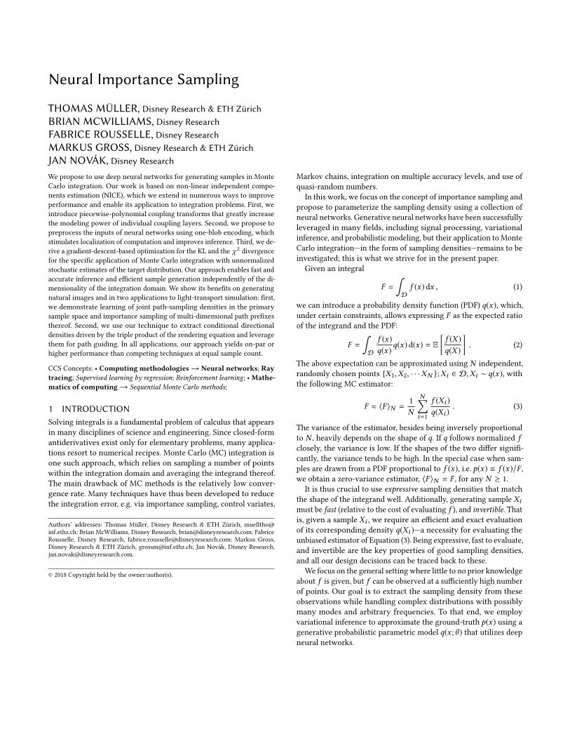
Fig. 1. A coupling layer splits the input x into two partitions A and B . Onepartition is left untouched, whereas dimensions in the other partition are

warped using a parametric coupling transform C driven by the output of a

neural networkm. Multiple coupling layers may need to be compounded

to achieve truly expressive transforms.

The invertibility is crucial in our setting as we require both density

estimation and sample generation in Monte Carlo integration.

The second important property of C is separability. Separable Censures that the Jacobian matrix is triangular and the determinant

reduces to the product of diagonal terms; see Dinh et al. [2014] or

Appendix A for a full treatment. The computation of the determinant

thus scales linearly with D and is therefore tractable even in high-

dimensional problems.

3.2 Affine Coupling Transforms

Additive Coupling Transform. Dinh et al. [2014] describe a very

simple coupling transform that merely translates the signal in indi-

vidual dimensions of B:

C(xB ; t) = xB + t , (10)

where the translation vector t ∈ R |B |is produced by functionm(xA).

Multiply-add Coupling Transform. Since additive coupling layers

have unit Jacobian determinants, i.e. they preserve volume, Dinh

et al. [2016] propose to add a multiplicative factor es :

C(xB ; s, t) = xB ⊙ es + t , (11)

where ⊙ represents element-wise multiplication and vectors t and

s ∈ R |B |are produced bym: (s, t) =m(xA). The Jacobian determi-

nant of a multiply-add coupling layer is simply exp

∑si .

The coupling transforms above are relatively simple. The trick

that enables learning nonlinear dependencies across partitions isthe parametric functionm. This function can be arbitrarily complex,

e.g. a neural network, as we do not need its inverse to invert the

coupling layer and its Jacobian does not affect the determinant

of the coupling layer (cf. Appendix A). Using a sophisticated mallows extracting complex nonlinear relations between the two

partitions. The coupling transform C , however, remains simple,

invertible, and permits tractable computation of determinants even

in high-dimensional settings.

3.3 Compounding Multiple Coupling Layers

As mentioned initially, the complete transform between the data

space and the latent space is obtained by chaining a number of cou-

pling layers. A different instance of neural networkm is trained for

each coupling layer. To ensure that all dimensions can be modified,


0.0 0.2 0.4 0.6 0.8 1.0

0

1

2

3

0.0 0.2 0.4 0.6 0.8 1.0

0

1

0.00 0.20 0.40 0.55 0.70 1.00

0

1

2

3

0.00 0.20 0.40 0.55 0.70 1.00

0

1

Target

Fit

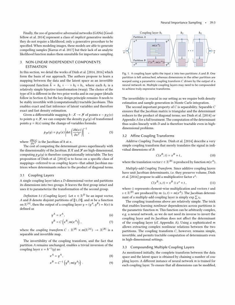
Network prediction: qi =∂Ci (x

Bi )

∂xBiCoupling transform: Ci (xBi )

P/w-linear

P/w-quadratic

Fig. 2. Predicted probability density functions (PDFs, left) and correspond-

ing cumulative distribution functions (CDFs, right) with K = 5 bins fitted to

a target distribution (dashed). The top row illustrates a piecewise-linear CDF

and the bottom row a piecewise-quadratic CDF. The piecewise-quadratic

approximation tends to work better in practice thanks to its first-order conti-

nuity (C1) and adaptive bin sizing. In Appendix B we show that, in contrast

to piecewise-quadratic CDFs, adaptive bin sizing is difficult to achieve for

piecewise-linear CDFs with gradient based optimization methods.

the output of one layer is fed into the next layer with the roles of the

two partitions swapped; see Figure 1. Compounding two coupling

layers in this manner ensures that every dimension can be altered.

The number of coupling layers required to ensure that each dimen-

sion can influence every other dimension depends on the total num-

ber of dimensions. For instance, in a 2D setting (where each partition

contains exactly one dimension) we need only two coupling layers.

3D problems require three layers, and for any high-dimensional

configuration there must be at least four coupling layers.

In practice, however, high-dimensional problems (e.g. generat-

ing images of faces), require significantly more coupling layers

since each affine transform is fairly limited. In the next section,

we address this limitation by providing more expressive mappings

that allow reducing the number of coupling layers and thereby the

sample-generation and density-estimation costs. This improves the

performance of Monte Carlo estimators presented in Section 6.

4 PIECEWISE-POLYNOMIAL COUPLING LAYERS

In this section, we propose piecewise-polynomial, invertible maps

as coupling transforms instead of the limited affine warps reviewed

previously. In contrast to Dinh et al. [2014, 2016], who assume

x,y ∈ (−∞,+∞)D and gaussian latent variables, we choose to oper-

ate in a unit hypercube (i.e. x,y ∈ [0, 1]D ) with uniformly distributed

latent variables, as most practical problems span a finite domain.

Unbounded domains can still be handled by warping the input of

h1 and the output of hL e.g. using the sigmoid and logit functions.

Similarly to Dinh and colleagues, we ensure computationally

tractable Jacobians via separability, i.e. C(xB ) =∏ |B |

i=1Ci (xBi ). Op-

erating on unit intervals allows interpreting the warping function

Ci as a cumulative distribution function (CDF). To produce each Ci ,we instrument the neural network to output the corresponding un-

normalized probability density qi , and construct Ci by integration;

see Figure 2 for an illustration.

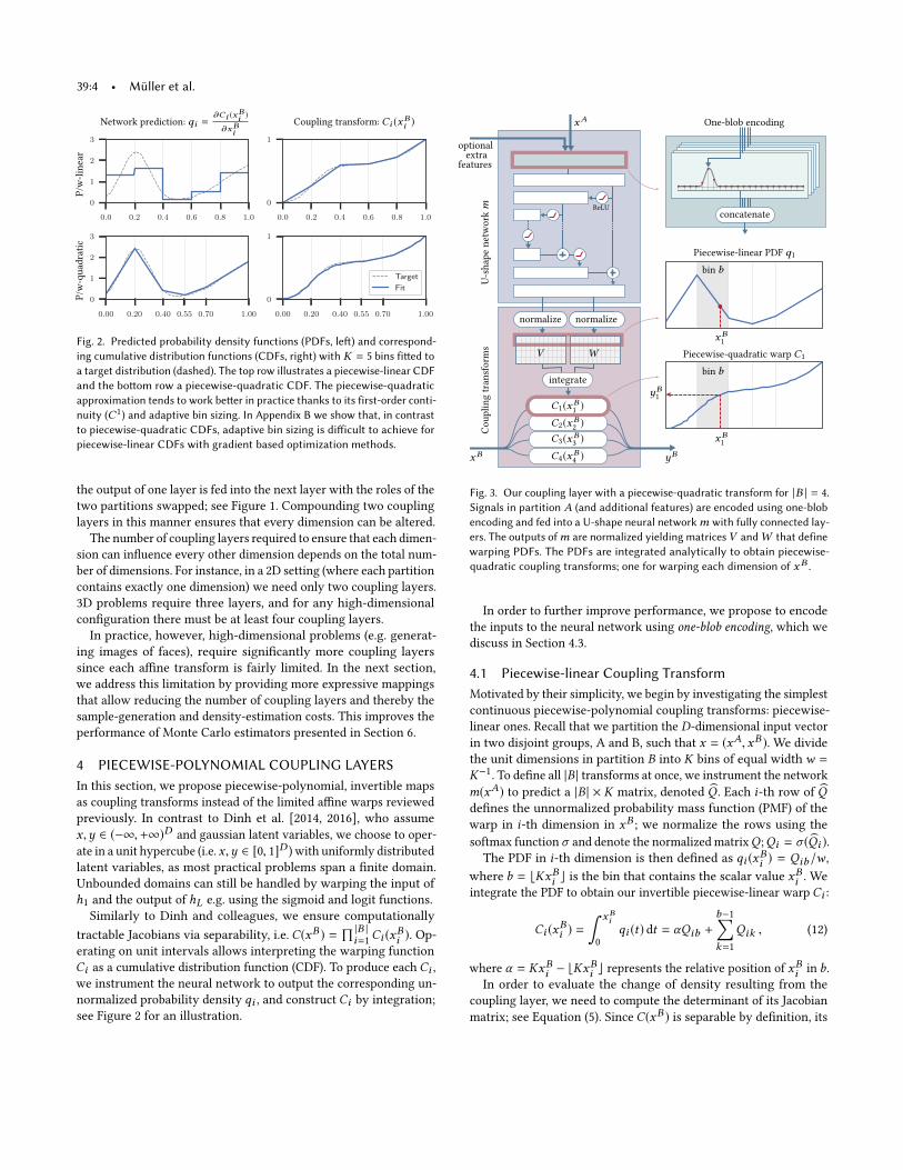
normalizenormalize

integrate

concatenate

normalize

U-shapenetworkm

Couplingtransforms

optional

extra

features

xA One-blob encoding

Piecewise-linear PDF q1

xB1

bin b

Piecewise-quadratic warp C1

xB1

yB1

bin b

V W

xB yB

normalize normalize

integrate

concatenate

C1(xB1)

C2(xB2)

C3(xB3)

C4(xB4)

ReLU

Fig. 3. Our coupling layer with a piecewise-quadratic transform for |B | = 4.

Signals in partition A (and additional features) are encoded using one-blob

encoding and fed into a U-shape neural networkm with fully connected lay-

ers. The outputs ofm are normalized yielding matricesV andW that define

warping PDFs. The PDFs are integrated analytically to obtain piecewise-

quadratic coupling transforms; one for warping each dimension of xB .

In order to further improve performance, we propose to encode

the inputs to the neural network using one-blob encoding, which we

discuss in Section 4.3.

4.1 Piecewise-linear Coupling Transform

Motivated by their simplicity, we begin by investigating the simplest

continuous piecewise-polynomial coupling transforms: piecewise-

linear ones. Recall that we partition the D-dimensional input vector

in two disjoint groups, A and B, such that x = (xA, xB ). We divide

the unit dimensions in partition B into K bins of equal widthw =K−1

. To define all |B | transforms at once, we instrument the network

m(xA) to predict a |B | × K matrix, denoted Q . Each i-th row of Qdefines the unnormalized probability mass function (PMF) of the

warp in i-th dimension in xB ; we normalize the rows using the

softmax function σ and denote the normalized matrixQ ;Qi = σ (Qi ).

The PDF in i-th dimension is then defined as qi (xBi ) = Qib/w ,

where b = ⌊KxBi ⌋ is the bin that contains the scalar value xBi . We

integrate the PDF to obtain our invertible piecewise-linear warp Ci :

Ci (xBi ) =

∫ xBi

0

qi (t) dt = αQib +

b−1∑k=1

Qik , (12)

where α = KxBi − ⌊KxBi ⌋ represents the relative position of xBi in b.In order to evaluate the change of density resulting from the

coupling layer, we need to compute the determinant of its Jacobian

matrix; see Equation (5). Since C(xB ) is separable by definition, its


Dinh et al. [2016] Ours (L=2)

Affine (L=2) Affine (L=4) Affine (L=16) P/w-linear P/w-quadratic Reference KL divergence Variance

100

102

Affine 2

Affine 4

Affine 16

P/w linear

P/w quad.

10−1

101

103

0 2.5k 5k

Training steps

0 2.5k 5k

Training steps

10−1

100

101

Fig. 4. Our 32-bin piecewise-linear (4-th column) and 32-bin piecewise-quadratic (5-th column) coupling layers achieve superior performance compared to

affine (multiply-add) coupling layers [Dinh et al. 2016] on low-dimensional density-estimation problems. The false-colored distributions were obtained by

optimizing KL divergence with uniformly drawn samples (weighted by the reference value) over the 2D image domain. The plots on the right show the training

error (KL divergence) and the variance obtained when using the distribution to importance-sample a Monte Carlo estimator of the average image color.

Affine (L=16) Piecewise-linear (L=2) Piecewise-quadratic (L=2)

scalar encoding one-blob encoding scalar encoding one-blob encoding scalar encoding one-blob encoding Reference

Fig. 5. Comparison of results with and without the one-blob encoding. The experimental setup is the same as in Figure 4. While the affine coupling transforms

fail to converge with one-blob encoded inputs, the distributions learned by the piecewise-polynomial coupling functions become sharper and more accurate.

Jacobian matrix is diagonal and the determinant is equal to the

product of the diagonal terms. These can be computed using Q :

det

©«∂C

(xB ;m(xA)

)∂(xB

)T ª®®¬ =|B |∏i=1

qi (xBi ) =

|B |∏i=1

Qibw, (13)

whereb again denotes the bin containing the value in the i-th dimen-

sion. To reduce the number of binsK required for a good fitwewould

like the network to also predict bin widths. These can unfortunately

not easily be optimized with gradient descent in the piecewise-linearcase; see Appendix B. To address this, and to improve accuracy, we

propose piecewise-quadratic coupling transforms.

4.2 Piecewise-quadratic Coupling Transform

Piecewise-quadratic coupling transforms admit a piecewise-linear

PDF, which we model using K + 1 vertices; see Figure 2, bottom left.

We store their vertical coordinates (for all dimensions in B) in |B | ×(K + 1) matrix V , and horizontal differences between neighboring

vertices (bin widths) in |B | × K matrixW .

The network m outputs unnormalized matrices W and V . We

again normalize thematrices using the standard softmaxWi = σ (Wi ),

and an adjusted version in the case of V :

Vi , j =exp

(Vi , j

)∑Kk=1

exp

(Vi ,k

)+exp

(Vi ,k+1

)2

Wi ,k

, (14)

where the denominator ensures that Vi represents a valid PDF.

The PDF in dimension i is defined as

qi (xBi ) = lerp(Vib ,Vib+1,α) , (15)

where α = (xBi −∑b−1k=1Wik )/Wib represents the relative position of

scalar xBi in bin b that contains it, i.e.

∑b−1k=1Wik ≤ xBi <

∑bk=1Wik .

The invertible coupling transform is obtained by integration:

Ci (xBi ) =

α2

2

(Vib+1 −Vib ) + αVib +b−1∑k=1

Vik +Vik+12

Wik . (16)

Note that invertingCi (xBi ) involves solving the root of the quadratic

term, which can be done efficiently and robustly.

Computing the determinant of the Jacobian matrix follows the

same logic as in the piecewise-linear case, with the only difference

being that we must now interpolate the entries of V in order to

obtain the PDF value at a specific location (cf. Equation (15)).


Examples from the training set Generated novel images Manifold spanned by four images

Fig. 6. Generative modeling of facial photographs using the architecture of Dinh et al. [2016] with our piecewise-quadratic coupling transform. We show

training examples (left), faces generated by our trained model (middle), and a manifold of faces spanned by linear interpolation of 4 training examples in

latent space (right). We achieve results of slightly better quality than Dinh et al. [2016], suggesting that our approach could benefit also high-dimensional

problems, though one may not achieve the same magnitude of improvements as in low-dimensional settings.

4.3 One-blob Encoding

An important consideration is the encoding of the inputs to the

network. We propose to use the one-blob encoding—a generalizationof the one-hot encoding—where a kernel is used to activate multiple

adjacent entries instead of a single one. Assume a scalar s ∈ [0, 1] and

a quantization of the unit interval into k bins (we use k = 32). The

one-blob encoding amounts to placing a kernel (we use a Gaussian

withσ = 1/k) at s and discretizing it into the bins.With the proposed

architecture of the neural network (placement of ReLUs in particular,

see Figure 3), the one-blob encoding effectively shuts down certain

parts of the linear path of the network, allowing it to specialize the

model on various sub-domains of the input.

In contrast to one-hot encoding, where the quantization causes a

loss of information if applied to continuous variables, the one-blob

encoding is lossless; it captures the exact position of s .

4.4 Analysis

We compare the proposed piecewise-polynomial coupling trans-

forms to multiply-add affine transforms [Dinh et al. 2016] on a 2D

density-estimation problem in Figure 4. To produce columns 1–5,

we uniformly sample the 2D domain, evaluate the reference func-

tion (column 6) at each sample, and optimize the neural networks

that control the coupling transforms using KL divergence described

in Section 5.1. Every per-layer network has a U-net (see Figure 3)

with 8 fully connected layers, where the outermost layers contain

256 neurons and the number of neuron is halved at every nesting

level. We use 2 additional layers to adapt the input and output di-

mensionalities to and from 256, respectively. The networks only

differ in their output layer to produce the desired parameters of

their respective coupling transform (s and t , Q , or W and V ).

We use adaptive bin sizes only in the piecewise-quadratic cou-

pling transforms because gradient descent fails to optimize them in

the piecewise-linear case as demonstrated in Appendix B.

When using L = 2 coupling layers—i.e. 2 × 10 fully connected

layers—the piecewise-polynomial coupling layers consistently per-

form better thanks to their significantly larger modeling power,

and outperform even large numbers (e.g. L = 16) of multiply-add

coupling layers, amounting to 16 × 10 fully connected layers.

Figure 5 demonstrates the benefits of the one-blob encoding when

combined with our piecewise coupling transforms. While the en-

coding helps our coupling transforms to learn sharp, non-linear

functions more easily, it also causes the multiply-add transforms of

Dinh et al. [2016] to produce excessive high frequencies that inhibit

convergence. Therefore, in the rest of the paper we use the one-blob

encoding only with our piecewise-polynomial transforms; results

with affine transforms do not utilize one-blob encoded inputs.

We tested the piecewise-quadratic coupling layers also on a high-

dimensional density-estimation problem: learning the manifold of a

specific class of natural images. We used the CelebFaces Attributes

dataset [Liu et al. 2015] and reproduced the experimental setting of

Dinh et al. [2016]. Our architecture is based on the authors’ publicly

available implementation and differs only in the coupling layer

used and the depth of the network—we use 4 recursive subdivisions

while the authors use 5, resulting in 28 versus 35 coupling layers. We

chose K = 4 bins and did not use our one-blob encoding due to GPUmemory constraints. Since our coupling layers operate on the [0, 1]D

domain, we do not use batch normalization on the transformed data.

Figure 6 shows a sample of the training set, a sample of gen-

erated images, and a visualization of the manifold given by four

different faces. The visual quality of our results is comparable to

those obtained by Dinh and colleagues. We perform marginally bet-

ter in terms of the bits-per-dimension metric (lower means better):

we yield 2.85 and 2.89 bits on training and validation data, respec-

tively, whereas Dinh et al. [2016] reported 2.97 and 3.02 bits. We

tried decreasing the number of coupling layers while increasing the

number of bins within each of them, but the results became overall

worse. We hypothesize that the high-dimensional problem of learn-

ing distributions of natural images benefits more from having many

coupling layers rather than having fewer but expressive ones.


5 MONTE CARLO INTEGRATION WITH NICE

In this section, we reduce the variance of Monte Carlo integration by

extracting sampling PDFs from observations of the integrand. Denot-

ing q(x ;θ ) the to-be-learned PDF for drawing samples (θ represents

the trainable parameters) and p(x) the ground-truth distribution of

the integrand, we can rewrite the MC estimator from Equation (3) as

⟨F ⟩N =1

N

N∑i=1

f (Xi )

q(Xi ;θ )=

1

N

N∑i=1

p(Xi ) F

q(Xi ;θ ). (17)

In the ideal case when q(x ;θ ) = p(x), the estimator returns the exact

value of F . Our objective here is to leverage NICE to learn q fromdata while optimizing the neural networks in coupling layers so

that the distance between p and q is minimized.

We follow the standard approach of quantifying the distance using

one of the commonly used divergence metrics. While all divergence

metrics reach their minimum if both distributions are equal, they

differ in shape and therefore produce different q in practice.

In Section 5.1, we optimize using the popular Kullback-Leibler

(KL) divergence. We further consider directly minimizing the vari-

ance of the resulting MC estimator in Section 5.2 and demonstrate

that it is equivalent to minimizing the χ2 divergence.

5.1 Minimizing Kullback-Leibler Divergence

Most generative models based on deep neural networks do not

allow evaluating the likelihoodq(x ;θ ) of data points x exactly and/or

efficiently. In contrast, our work is based on bijective mappings with

tractable Jacobian determinants that easily permit such evaluations.

In the following, we show that using the KL divergencewith gradient

descent amounts to directly maximizing a weighted log likelihood.

The KL divergence between p(x) and the learned q(x ;θ ) reads

DKL(p ∥ q;θ ) =

∫Ωp(x) log

p(x)

q(x ;θ )dx

=

∫Ωp(x) logp(x) dx −

∫Ωp(x) logq(x ;θ ) dx︸︷︷︸Cross entropy

. (18)

To minimize DKL with gradient descent, we need its gradient with

respect to the trainable parameters θ . These appear only in the

cross-entropy term, hence

∇θDKL(p ∥ q;θ ) = −∇θ

∫Ωp(x) logq(x ;θ ) dx (19)

= E

[−

p(X )

q(X ;θ )∇θ logq(X ;θ )

], (20)

where the expectation is overX ∼ q(x ;θ ), i.e. the samples are drawn

from the learned generative model1. In most integration problems,

p(x) is only accessible in an unnormalized form through f (x):p(x) =f (x)/F . Since F is unknown—this is what we are trying to estimate

in the first place—the gradient can be estimated only up to the global

scale factor F . This is not an issue since common gradient-descent-

based optimization techniques such as Adam [Kingma and Ba 2014]

scale the step size by the reciprocal square root of the gradient

1If samples could be drawn directly from the ground-truth distribution—as is common

in computer vision problems—the stochastic gradient would simplify to that of just the

log likelihood. We discuss a generalization of log-likelihood maximization.

variance, cancelling F . Furthermore, if f (x) can only be estimated

via Monte Carlo, the gradient is still correct due to the linearity of

expectations. Equation (20) therefore shows that minimizing the

KL divergence via gradient descent is equivalent to minimizing the

negative log likelihood weighted by MC estimates of F .

5.2 Minimizing Variance via χ 2 Divergence

Themost attractive quantity to minimize in the context of (unbiased)

Monte Carlo integration is the variance of the estimator. Inspired by

previous works that strive to directly minimize variance [Pantaleoni

and Heitz 2017; Vévoda et al. 2018], we demonstrate how this can be

achieved for the MC estimator p(X )/q(X ;θ ), with X ∼ q(x ;θ ), viagradient descent. We begin with the variance definition and simplify:

V

[p(X )

q(X ;θ )

]= E

[p(X )2

q(X ;θ )2

]− E

[p(X )

q(X ;θ )

]2

=

∫Ω

p(x)2

q(x ;θ )dx −

(∫Ωp(x) dx

)2

︸︷︷︸1

. (21)

The stochastic gradient of the variance for gradient descent is then

∇θV

[p(X )

q(X ;θ )

]= ∇θ

∫Ω

p(x)2

q(x ;θ )dx

=

∫Ωp(x)2 ∇θ

1

q(x ;θ )dx

=

∫Ω−p(x)2

q(x ;θ )∇θ logq(x ;θ ) dx

= E

[−

(p(X )

q(X ;θ )

)2

∇θ logq(X ;θ )

]. (22)

Relation to the Pearson χ2 divergence. Upon close inspection it

turns out the variance objective (Equation 21) is equivalent to the

Pearson χ2 divergence Dχ 2 (p ∥ q;θ ):

Dχ 2 (p ∥ q;θ ) =

∫Ω

(p(x) − q(x ;θ ))2

q(x ;θ )dx

=

∫Ω

p(x)2

q(x ;θ )dx −

(2

∫Ωp(x) dx −

∫Ωq(x ;θ ) dx

)︸︷︷︸

1

.

(23)

As such,minimizing the variance of aMonte Carlo estimator amounts

to minimizing the Pearson χ2 divergence between the ground-truth

and the learned distributions.

Connection between the χ2 and KL divergences. Notably, the gra-dients of the KL divergence and the χ2 divergence differ only in the

weight applied to the log likelihood. In ∇θDKL the log likelihood is

weighted by the MC weight, whereas when optimizing ∇θDχ 2 , the

log likelihood is weighted by the squared MCweight. This illustrates

the difference between the two loss functions: the χ2 divergencepenalizes large discrepancies stronger, specifically, low values of

q in regions of large density p. As such, it tends to produce more

conservative q than DKL, which we observe in Section 6 as fewer

outliers at the cost of slightly worse average performance.


6 NEURAL PATH SAMPLING AND PATH GUIDING

In this section, we take NICE (Section 3) with piecewise-polynomial

warps (Section 4) and apply it to sequential MC integration of light

transport using the methodology described in Section 5. Our goal is

to reduce estimation variance by “guiding” the construction of light

paths using on-the-fly learned sampling densities. We explore two

different settings: a global setting that leverages the path-integral

formulation of light transport and employs high-dimensional sam-

pling in the primary sample space (PSS) to build complete light-path

samples (Section 6.1), and a local setting, natural to the rendering

equation, where the integration spans a 2D (hemi-)spherical domain

and the path is built incrementally (Section 6.2).

6.1 Primary-Sample-Space Path Sampling

In order to produce an image, a renderer must estimate the amount

of light reaching the camera after taking any of the possible paths

through the scene. The transport can be formalized using the path-

integral formulation [Veach 1997], where a radiance measurement

I to a sensor (e.g. a pixel) is given by an integral over path space P:

I =

∫P

Le(x0, x1)T (x)W (xk−1, xk ) dx . (24)

The chain of positions x = x0 · · · xk represents a single light path

with k vertices. The path throughputT (x) quantifies the ability of xto transport radiance. Le quantifies emitted radiance andW is the

sensor response to one unit of incident radiance.

The measurement can be estimated as

⟨I ⟩ =1

N

N∑j=1

Le(xj0, xj1)T (x j )W (xjk−1, xjk )q(x j )

, (25)

whereq(x) is the joint probability density of generating all k vertices

of path x . Drawing samples directly from the joint distribution is

challenging due to the constrained nature of vertices; e.g. they have

to reside on surfaces. Several approaches thus propose to operate

in the primary sample space (PSS) [Guo et al. 2018; Kelemen et al.

2002] represented by a unit hypercubeU. A path is then obtained

by transforming a vector of random numbers z ∈ U using one of

the standard path-construction techniques ρ (e.g. camera tracing):

x = ρ(z).Operating in PSS has a number of compelling advantages. The

sampling routine has to be evaluated only once per path, instead

of once per path vertex, and the generic nature of PSS coordinates

enables treating the path construction as a black box. Importance

sampling of paths can thus be applied to any single path-tracing

technique, and, with some effort, also to multiple strategies [Guo

et al. 2018; Hachisuka et al. 2014; Kelemen et al. 2002; Lafortune and

Willems 1995; Veach and Guibas 1994]. Lastly, the sampling routine

directly benefits from existing importance-sampling techniques in

the underlying path-tracing algorithm since those make the path-

contribution function smoother in PSS and thus easier to learn.

Methodology. Given that NICE scales well to high-dimensional

problems, applying it in PSS is straightforward. We split the di-

mensions of U into two equally-sized groups A and B, where Acontains the even dimensions and B contains the odd dimensions.

One group serves as the input of the neural network (each dimension

is processed using the one-blob encoding) while the other group is

being warped; their roles are swapped in the next coupling layer.

To infer the parameters θ of the networks, we minimize one of the

losses from Section 5 against p(x) = Le(x0, x1)T (x)W (xk−1, xk ) F−1,ignoring the unknown normalization factor, i.e. assuming F = 1.

In order to obtain a path sample x , we generate a random vector

z, warp it using the reversed inverted coupling layers, and apply the

path-construction technique: x = ρ(h−11

(· · ·h−1L (z)

)); please refer

back to Equation (8) and (9) for details on the inverses.

Before we analyze the performance of primary-sample-space path

sampling in Section 6.4, we discuss a slightly different approach

to data-driven construction of path samples—the so-called path

guiding—which applies neural importance sampling at each vertex

of the path and typically yields higher performance.

6.2 Path Guiding

A popular alternative to formalizing light transport using the path-

integral formulation is to adopt a local view and focus on the radia-

tive equilibrium of individual points in the scene. The equilibrium

radiance at a surface point x in directionωo is given by the rendering

equation [Kajiya 1986]:

Lo(x,ωo) = Le(x,ωo) +

∫ΩL(x,ω)fs(x,ωo,ω)| cosγ | dω , (26)

where fs is the bidirectional scattering distribution function,Lo(x,ωo),

Le(x,ωo), and L(x,ω) are respectively the reflected, emitted, and in-

cident radiance, Ω is the unit sphere, and γ is the angle between ωand the surface normal.

The rendering task is formulated as finding the outgoing radiance

at points directly visible from the sensor. The overall efficiency

of the renderer heavily depends on the variance of estimating the

amount of reflected light:

⟨Lr(x,ωo)⟩ =1

N

N∑j=1

L(x,ωj )fs(x,ωo,ωj )| cosγj |

q(ωj |x,ωo). (27)

A large body of research has therefore focused on devising sampling

densities q(ω |x,ωo) that yield low variance. While the density is

defined over a 2D space, it is conditioned on position x and directionωo. These extra five dimensions make the goal of q(ω |x,ωo) ∝

L(x,ω)fs(x,ωo,ω)| cosγ | substantially harder.

Since the 7D domain is fairly challenging to handle using hand-

crafted, spatio-directional data structures in the general case, most

research has focused on the simpler 5D setting where q(ω |x,ωo) ∝

L(x,ω) [Dahm and Keller 2018; Hey and Purgathofer 2002; Jensen

1995; Müller et al. 2017; Pegoraro et al. 2008a,b; Vorba et al. 2014]

and only a few attempts have been made to consider the full prod-

uct [Herholz et al. 2018, 2016; Lafortune and Willems 1995; Stein-

hurst and Lastra 2006]. These path-guiding approaches rely on

carefully chosen data structures (e.g. BVHs, kD-trees) in combina-

tion with relatively simple PDF models (e.g. histograms, quad-trees,

gaussian mixture models), which are populated in a data-driven

manner either in a pre-pass or online during rendering. Our goal is

also to learn accurate local sampling densities, but we utilize NICE

to represent and sample from q(ω |x,ωo).


Methodology. We use a single instance of NICE, which is trained

and sampled from in an interleaved manner. In the most general

setting, we consider learning q(ω |x,ωo) that is proportional to the

product of all terms in the integrand. Since the integration domain

is only 2D, partitions A and B in all coupling layers contain only

one dimension each—one of the two cylindrical coordinates that we

use to parameterize the sphere of direction.

To produce the parameters of the first piecewise-polynomial cou-

pling function, the neural networkm takes the cylindrical coordinate

from A, the position x and direction ωo that condition the density,

and additional information that may improve inference; we also

input the normal of the intersected shape at x to aid the network in

learning distributions that correlate with the local shading frame.

We one-blob encode all of the inputs as described in Section 4.3

with k = 32. In the case of x, we normalize it by the scene bounding

box, encode each coordinate independently, and concatenate the re-

sults into a single array of 3×k values. We proceed analogously with

directions, which we parameterize using world-space cylindrical

coordinates: we transform each coordinate to [0, 1] interval, encode

it, and append to the array. The improved performance enabled by

our proposed one-blob encoding is reported in Table 1.

At any given point during rendering, a sample is generated by

drawing a random pair u ∈ [0, 1]2, passing it through the inverted

coupling layers in reverse order, h−11(· · ·h−1L (u)), and transforming

to the range of cylindrical coordinates to obtain ω.

MIS-aware Optimization. In order to optimize the networks, we

use Adam with one of the loss functions from Section 5, but with

an important, problem-specific alteration. To sample ω, most cur-

rent renderers apply multiple importance sampling (MIS) [Veach

and Guibas 1995] to combine multiple sampling densities (e.g. to

estimate direction illumination or importance sample the BSDF).

When learning the product, we take this into account by optimizing

the networks with respect to the final (MIS) PDF instead of the den-

sity learned using NICE. If certain parts of the product are already

covered well by existing densities, the networks will therefore be

optimized to only handle the remaining problematic case.

We therefore optimize D(p ∥ q′) where q′ = wq + (1 − w)pfsand p(ω |x,ωo) = L(x,ω)fs(x,ωo,ω)| cosγ |F

−1(we again ignore the

normalization constant F ) and pfs is the PDF for sampling the BSDF.

We use an additional network m to learn optimal MIS weights

w = l(m(x,ωo)) and optimize it jointly with the other networks; all

networks use the same architecture and l is the logistic function. Toprevent overfitting to local optima with degenerate MIS weights,

we use the loss funtion β(i)D(p ∥ q) + (1 − β(i))D(p ∥ q′) where i is

the current training iteration and β(i) = 1/2 · (1/3)i

1000 .

BSDFs that are a mixture of delta and smooth functions—such

as plastic—require a small amount of special handling. While our

stochastic gradient in Section 5 in theory is well behaved with delta

functions, they need to be treated as finite quantities in practice due

to the limitations of floating point numbers. When the path tracer

samples delta components, continuous densities therefore need to

be set to 0 and optimization of our coupling functions disabled (by

setting their loss to 0), effectively only optimizing for MIS weights.

Discussion. Our approach to sampling the full triple product

L(x,ωj )fs(x,ωo,ωj )| cosγj | has three distinct advantages. First, it isagnostic to the number of dimensions that the 2D domain is condi-

tioned on. This allows for high-dimensional conditionals without so-

phisticated data structures. One can simply input extra information

into the neural networks and let them learn which dimensions are

useful in which situations. While we only pass in the surface normal,

the networks could be supplied with additional information—e.g.

textured BSDF parameters—to further improve the performance in

cases where the product correlates with such information. In that

sense, our approach is more automatic then previous works.

The second advantage is that our method does not require any

precomputation, such as fitting of (scene-dependent) materials into

a mixture of gaussians [Herholz et al. 2018, 2016]. While a user still

needs to specify the hyper-parameters as is also required by most

other approaches, we found our configuration of hyperparameters

to work well across all tested scenes.

Lastly, our approach offers trivial persistence across renders. A set

of networks trained on one camera view can be easily reused from a

different view or within a slightly modified scene; we demonstrate

this in Section 6.4. Unlike previous approaches, where the learned

data structure requires explicit support of adaptation to new scenes,

neural networks can be adapted by the same optimization procedure

that was used in the initial training. Applying our approach to

animations could thus yield super-linear cost savings.

6.3 Experimental Setup

We implemented our technique in Tensorflow [Abadi et al. 2015] and

integrated it with the Mitsuba renderer [Jakob 2010]. Before we start

rendering, we initialize the trainable parameters of our networks us-

ing Xavier initialization [Glorot and Bengio 2010]. While rendering

the image, we optimize them using Adam [Kingma and Ba 2014].

Our rendering procedure is implemented as a hybrid CPU/GPU

algorithm, tracing rays in large batches on the CPU while two GPUs

perform all neural-network-related tasks. One GPU is responsible

for evaluating and sampling from q, while the other trains the net-works using Monte Carlo estimates from completed paths. Both

GPUs use minibatch sizes of 100 000 samples. Communication be-

tween the CPU and GPUs happens via asynchronous queues to aid

parallelization, where our training queue is additionally configured

to contain at least 1 000 000 elements before permitting dequeuing.

Each dequeued training minibatch then contains a random subset of

the queue’s elements to spread samples uniformly across the scene

as much as feasible. The other queue has no such constraints and is

processed as fast as possible.

In order to obtain the final image with N samples, we perform

M = ⌊log2(N + 1)⌋ iterations with power-of-two sample counts

2i; i ∈ 0, · · · ,M. This approach was initially proposed by Müller

et al. [2017] to limit the impact of initial high-variance estimates on

the final image. In contrast to their work, we do not reset the learned

distributions at every power-of-two iteration and keep training the

same set of networks from start to finish. Furthermore, instead of

discarding the samples of earlier iterations, we weight the images

produced within each iteration by their reciprocal mean pixel vari-

ance, which we estimate on-the-fly. While this approach introduces


Affine, L = 16 Ours, piecewise-quadratic, L = 4

PT-Unidir PSSPG—4D NPS—6D NPS—2D NPS—4D NPS—6D Reference

Bathroom

MAPE: 0.1466 0.1510 0.1554 0.1473 0.1455 0.1461

Spaceship

MAPE: 0.0424 0.0351 0.0418 0.0289 0.0294 0.0298

SwimmingPool

MAPE: 0.6915 0.4910 0.7878 0.1976 0.1675 0.1774

CopperHairball

MAPE: 0.4700 0.3145 0.2471 0.2210 0.1949 0.1915

CountryKitchen

MAPE: 0.6878 0.6465 0.6978 0.6783 0.6017 0.5673

Necklace

MAPE: 0.3590 0.3410 0.3613 0.2506 0.2686 0.2842

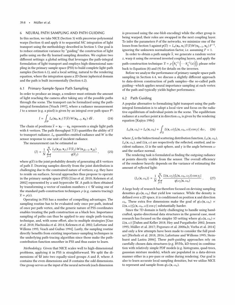
Fig. 7. Neural path sampling in primary sample space. We compare a standard uni-directional path tracer (PT-Unidir), the method by Guo et al. [2018]

(PSSPG), neural path sampling using L = 16 multiply-add coupling layers [Dinh et al. 2016], and L = 4 of our proposed piecewise-quadratic coupling layers,

both optimized using the KL divergence. We experimented with sampling the 1, 2, or 3 first non-specular bounces (NPS–2D, NPS–4D and NPS–6D). Overall,

our technique performs best in terms of mean absolute percentage error (MAPE) in this experiment, but only offers improvement beyond the 4D case if paths

stay coherent, e.g. in the top crop of the Spaceship scene. More results and error visualizations can be found in the supplemented image viewer.


Ours, KL divergence Ours, χ 2div.

PT-Unidir PPG GMM NPG-Radiance NPG-Product NPG-Product Reference

Bathroom

MAPE: 0.1466 0.1897 0.2718 0.1811 0.0507 0.0652

Spaceship

MAPE: 0.0424 0.0352 0.0640 0.0330 0.0189 0.0428

SwimmingPool

MAPE: 0.6915 0.0819 0.0772 0.0764 0.0679 0.0887

CopperHairball

MAPE: 0.4700 0.1337 0.1561 0.1406 0.0847 0.1294

CountryKitchen

MAPE: 0.6878 0.1241 0.1505 0.1184 0.0882 0.1609

Necklace

MAPE: 0.3590 0.1611 0.1612 0.1403 0.2332 0.2934

Fig. 8. Neural path guiding. We compare a uni-directional path tracer (PT-Unidir), the practical path-guiding (PPG) algorithm of Müller et al. [2017], the

gaussian mixture model (GMM) of Vorba et al. [2014], and variants of our framework with L = 4 coupling layers sampling the incident radiance alone (NPG-

Radiance) or the whole integrand (NPG-Product), when optimizing either the KL and χ 2divergences. Overall, sampling the whole integrand with the KL

divergence yields the most robust results. Note how optimizing the χ 2divergence tends to produce higher variance overall, but fewer outliers, in particular in

the Swimming Pool scene. More results and error visualizations can be found in the supplemented image viewer.


Cornell Box Country Kitchen Swimming Pool

GMM PPG NPG-Rad. Reference GMM PPG NPG-Rad. Reference GMM PPG NPG-Rad. Reference

Fig. 9. Directional radiance distributions. From left to right: we visualize the distributions learned by a gaussian mixture model (GMM) [Vorba et al. 2014], an

SDTree (PPG) [Müller et al. 2017], our neural path-guiding approach trained on radiance (NPG-Rad.), and a spatial binary tree with a directional regular

128 × 128 grid (Reference). The first three approaches were trained with an equal sample count and require roughly equal amounts of memory in the above

scenes (around 10 MB). We used 216

samples per pixel to generate the reference distributions, which require roughly 5GB per scene. Our approach not only

produces the most faithful distributions, but also—unlike the competing techniques—learns a continuous function in both the spatial and the directional

domain, requiring a smaller amount of blur. We illustrate the spatial continuity of our distributions in the supplementary video.

bias, it is imperceptibly small in practice due to averaging across all

pixels. Furthermore, the bias vanishes as the quality of the variance

estimate increases, making this approach consistent. We apply the

same weighting scheme to our implementation of the method by

Müller et al. [2017] to ensure a fair comparison.

All results were produced on a workstation with two Intel Xeon

E5-2680v3 CPUs (24 cores; 48 threads) and two NVIDIA Titan Xp

GPUs. Due to the combined usage of both the CPU and the GPU,

runtimes of different techniques depend strongly on the particular

setup. We therefore compare the performance using equal-sample-count metrics that are agnostic to used hardware. Absolute timings

are provided for completeness.

We quantify the error using the mean absolute percentage error(MAPE), which is defined as

1

N∑Ni=1 |vi − vi |/(vi + ϵ), where vi is

the value of the i-th pixel in the ground-truth image, vi is the valueof the i-th rendered pixel, and ϵ = 0.01 serves the dual objective

of avoiding the singularity at vi = 0 and down-weighting close-to-

black pixels. We use a relative metric to avoid putting overly much

emphasis on bright image regions. We also evaluated SMAPE, L1,

MRSE, L2, and SSIM, which all can be inspected as false-color maps

and aggregates in the supplemented image viewer.

6.4 Results

In order to best illustrate the benefits of different neural-importance-

sampling approaches, we compare their performance when used on

top of a unidirectional path tracer that uses BSDF sampling only.

While none of the results utilized next-event estimation (including

prior works), we recommend using it in practice for best perfor-

mance. In the following, all results with our piecewise-polynomial

coupling functions utilize L = 4 coupling layers. We use 512 spp

on all scenes except for the Copper Hairball (1024 spp) and Yet

Another Box (2048 spp). We also report the total sample count as

mega samples (MS) as it reflects the quality of learned distributions.

In Figure 7, we study primary-sample-space path sampling using

our implementation of the technique by Guo et al. [2018] (PSSPG)

and our neural path sampling (NPS) with piecewise-polynomial and

affine coupling transforms. We apply the sampling to only a limited

number of non-specular interactions in the beginning of each path

and sample all other interactions using uniform random numbers.

We experimented with three different prefix dimensionalities: 2D,

4D, and 6D, which correspond to importance sampling path prefixes

of 1, 2, and 3 non-specular vertices, respectively. As shown in the

figure, going beyond 4D brings typically little improvement, except

for the highlights in the Spaceship, where even longer paths are

correlated thanks to highly-glossy interactions with the glass of

the cockpit2. This confirms the observation of Guo et al. [2018]

that cases where more than two bounces are needed to connect to

the light source offer minor to no improvement. We speculate that

the poor performance in higher dimensions is due to the relatively

weak correlation between path geometries and PSS coordinates, i.e.

paths with similar PSS coordinates may have drastically different

vertex positions. The correlation tends to weaken at each additional

bounce (e.g. in the diffuse Cornell Box) unless the underlying path

importance-sampling technique preserves path coherence.

In Figure 8, we analyze the performance of different path-guiding

approaches, referring to ours as neural path guiding (NPG). We

compare our work to the respective authors’ implementations of

practical path guiding (PPG) by Müller et al. [2017] and the bidirec-

tionally trained gaussianmixture model (GMM) by Vorba et al. [2014]

which are both learning sampling distributions that are, in contrast

2Due to faster training of lower-dimensional distributions, the 2D case still has the

least overall noise in the Spaceship scene.


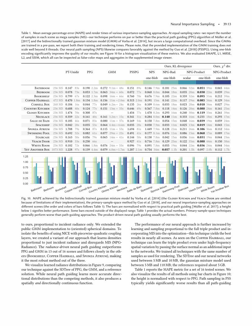
Table 1. Mean average percentage error (MAPE) and render times of various importance-sampling approaches. At equal sampling rates—we report the number

of samples in each scene as mega samples (MS)—our technique performs on par or better than the practical path guiding (PPG) algorithm of Müller et al.

[2017] and the bidirectionally trained gaussian mixture model (GMM) of Vorba et al. [2014], but incurs a large computational overhead. Since the GMMs

are trained in a pre-pass, we report both their training and rendering times. Please note, that the provided implementation of the GMM training does not

scale well beyond 8 threads. Our neural path sampling (NPS) likewise compares favorably against the method by Guo et al. [2018] (PSSPG). Using one-blob

encoding significantly improves the quality of our results; see Figure 10 for a histogram visualization of these metrics. We also evaluated SMAPE, L1, MRSE,

L2, and SSIM, which all can be inspected as false-color maps and aggregates in the supplemented image viewer.

Ours, KL divergence Ours, χ 2div.

PT-Unidir PPG GMM PSSPG NPS NPG-Rad. NPG-Product NPG-Product

one-blob one-blob scalar one-blob one-blob

Bathroom 236 MS 0.147 83s 0.190 2.2m 0.272 9.1m+ 48s 0.151 89s 0.146 7.9m 0.181 25m 0.066 32m 0.051 39m 0.065 44m

Bedroom 236 MS 0.078 73s 0.053 1.7m 0.063 34m + 60s 0.072 77s 0.068 8.0m 0.044 18m 0.035 20m 0.030 22m 0.039 29m

Bookshelf 236 MS 0.799 67s 0.122 2.3m 0.098 16m + 66s 0.760 78s 0.676 7.9m 0.105 22m 0.359 32m 0.095 31m 0.212 39m

Copper Hairball 472 MS 0.470 1.8m 0.134 1.8m 0.156 11m +2.0m 0.315 2.0m 0.191 15m 0.141 22m 0.117 29m 0.085 34m 0.129 34m

Cornell Box 268 MS 0.184 16s 0.044 77s 0.049 6.2m+ 24s 0.135 26s 0.109 8.6m 0.033 18m 0.023 28m 0.018 34m 0.027 29m

Country Kitchen 236 MS 0.688 40s 0.124 77s 0.151 13m + 33s 0.646 49s 0.567 7.8m 0.118 14m 0.126 20m 0.088 24m 0.161 25m

Glossy Kitchen 236 MS 1.474 70s 0.308 87s — 1.454 77s 1.478 8.2m 0.293 16m 0.240 30m 0.119 33m 0.261 39m

Necklace 236 MS 0.359 22s 0.161 40s 0.161 3.2m+ 15s 0.341 31s 0.284 8.0m 0.140 11m 0.333 16m 0.233 18m 0.293 17m

Salle de Bain 236 MS 0.185 46s 0.071 83s 0.080 11m + 37s 0.169 54s 0.158 7.8m 0.054 15m 0.048 16m 0.039 19m 0.059 24m

Spaceship 236 MS 0.042 20s 0.035 53s 0.064 4.4m+4.6m 0.035 28s 0.030 7.9m 0.033 11m 0.025 13m 0.019 14m 0.043 15m

Sponza Atrium 236 MS 1.708 79s 0.364 87s 0.115 11m + 53s 1.694 81s 1.449 7.9m 0.128 21m 0.211 26m 0.106 36m 0.112 34m

Swimming Pool 236 MS 0.692 32s 0.082 61s 0.077 29m + 22s 0.491 41s 0.177 8.1m 0.076 11m 0.086 15m 0.068 17m 0.089 17m

Staircase 236 MS 0.163 50s 0.056 79s 0.065 14m + 41s 0.144 58s 0.130 7.8m 0.042 15m 0.036 16m 0.031 19m 0.044 23m

Veach Door 236 MS 0.910 33s 0.230 66s — 0.927 41s 0.716 7.8m 0.129 25m 0.122 35m 0.088 44m 0.150 38m

White Room 236 MS 0.102 72s 0.066 1.8m 0.076 24m + 55s 0.096 79s 0.091 7.8m 0.055 19m 0.044 22m 0.036 24m 0.044 34m

Yet Another Box 1073 MS 1.228 97s 0.139 4.4m 0.079 6.0m+1.7m 1.207 2.1m 0.754 34m 0.057 1.1h 0.201 1.5h 0.097 2.0h 0.112 1.7h

BathroomBedroom

Bookshelf

Copper Hairball

Cornell Box

Country Kitchen

Glossy KitchenNecklace

Salle de BainSpaceship

Sponza Atrium

Swimming Pool

StaircaseVeach Door

White Room

Yet Another Box0.00

0.25

0.50

0.75

1.00

1.25

Fig. 10. MAPE achieved by the bidirectionally trained gaussian mixture model by Vorba et al. [2014] (the Glossy Kitchen and Veach Door are omitted

because of limitations of their implementation), the primary-sample-space method by Guo et al. [2018], and our neural importance-sampling approaches on

different scenes (the order and colors of bars follows Table 1). The bars are normalized with respect to practical path guiding [Müller et al. 2017]; a height

below 1 signifies better performance. Some bars exceed outside of the displayed range; Table 1 provides the actual numbers. Primary-sample-space techniques

generally perform worse than path-guiding approaches. The product-driven neural path guiding usually performs the best.

to ours, proportional to incident radiance only. We extended the

public GMM implementation to (oriented) spherical domains. To

isolate the benefits of using NICE with piecewise-quadratic coupling

layers, we created a variant of our approach that learns densities

proportional to just incident radiance and disregards MIS (NPG-

Radiance). The radiance-driven neural path guiding outperforms

PPG and GMM in 13 out of 16 scenes and follows closely in the oth-

ers (Bookshelf, Copper Hairball, and Sponza Atrium), making

it the most robust method out of the three.

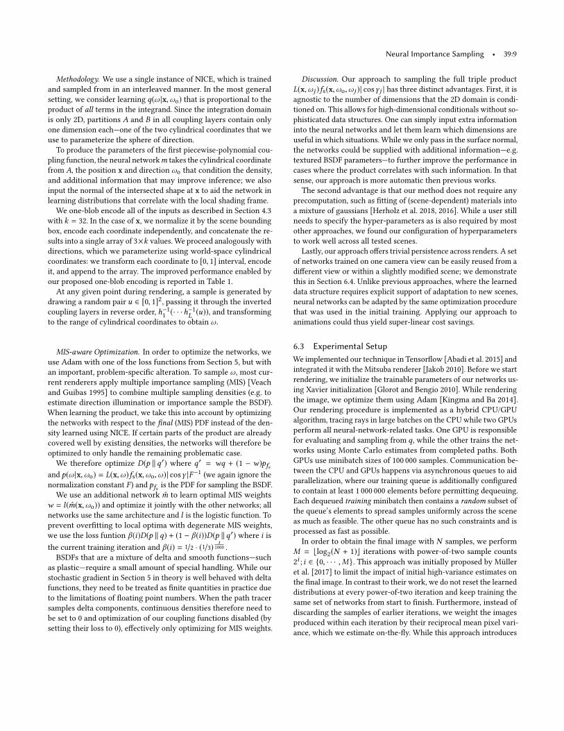
We visualize learned radiance distributions in Figure 9, comparing

our technique against the SDTree of PPG, the GMM, and a reference

solution. While neural path guiding learns more accurate direc-

tional distributions than the competing methods, it also produces a

spatially and directionally continuous function.

The performance of our neural approach is further increased by

learning and sampling proportional to the full triple product and in-

corporatingMIS into the optimization—this technique yields the best

results in nearly all scenes. As seen on the Copper Hairball, our

technique can learn the triple product even under high-frequency

spatial variation by passing the surface normal as an additional input

to the networks. We trained all techniques with the same number of

samples as used for rendering. The SDTree and our neural networks

used between 5MB and 10MB, the gaussian mixture model used

between 5MB and 118MB; the references required about 5GB.

Table 1 reports the MAPE metric for a set of 16 tested scenes. We

also visualize the results of all methods using bar charts in Figure 10;

the height is normalized with respect to PPG. Path sampling in PSS

typically yields significantly worse results than all path-guiding


Fixed weights Learned weights

Fig. 11. Learning MIS weights—even with product-driven path guiding—

leads to significantly better results on the Spaceship cockpit, where BSDF

sampling is near optimal.

approaches. Neural path guiding always benefits (sometimes sig-

nificantly) from encoding the inputs with one-blob encoding as

opposed to inputing raw (scalar) values.

We also compared variants of product-driven neural path guid-

ing optimized using the Kullback-Leibler (KL) and χ2 divergencesduring training. The squared Monte Carlo weight in the χ2 gradientcauses a large variance, making it difficult to optimize with. We

remedy this problem by clipping the minibatch gradient norm to

a maximum of 50. While the χ2 divergence in theory minimizes

the estimator variance most directly (see Section 5.2), it performed

worse in practice according to the MAPE metric on all test scenes.

A notable aspect of optimizing the χ2 divergence is that it tends toproduce results with higher variance overall, but fewer outliers, e.g.

in the Sponza Atrium and Swimming Pool scenes.

In Figure 11, we demonstrate the increased robustness of neural

path guiding offered by optimizing MIS weights. The impact is par-

ticularly noticeable on the cockpit of the spaceship seen through

specular interactions, which are handled nearly optimally by sam-

pling the material BSDF. In this region, a standard path tracer out-

performs the learned sampling PDFs. With learned MIS weights,

the system downweights the contribution of the learned PDF on

the cockpit, but increases it in regions where it is more accurate,

resulting in significantly improved results overall.

Figure 12 demonstrates the benefits of reusing networks, opti-

mized for a particular camera view, in a novel view of the scene.

We took network weights that resulted from generating images for

Figure 8 as the initial weights for rendering images in the right

column of Figure 12. Similarly to training from scratch, we keep op-

timizing the networks. If the initial distributions are already a good

fit, our weighting scheme by the reciprocal mean pixel variance

automatically keeps initial samples rather than discarding them.

7 DISCUSSION AND FUTURE WORK

Speed. An important property of practical sampling strategies

is a low computational cost of generating samples and evaluating

their PDF, relative to the cost of evaluating the integrand. In our

path-guiding applications, the cost is dominated by the evaluation

of coupling layers. Roughly 1/4 of the time is spent performing the

one-blob encoding, 2/4 in fully connected layers, and finally 1/4 per-

forming the piecewise-polynomial warp. This makes the overhead

of our implementation prohibitive in simple scenes. While we fo-

cused on the theoretical challenge of applying neural networks to

From scratch Reused

Spaceship

SwimmingPool

CountryKitchen

Fig. 12. Learned distributions can be reused for novel camera views. The

right column shows results where the network weights were initialized with

weights learned for camera views in Figure 8.

the problem of importance sampling in this work, accelerating the

computation to make our approach more practical is an important

and interesting future work. We believe specialized hardware (e.g.

NVIDIA’s TensorCores) and automatic computation graph optimiza-

tion (e.g. NVIDIA’s TensorRT) are promising next steps, which alone

might be enough to bring our approach into the realm of practicality.

Optimizing for Multiple Integrals. In Section 5.1, we briefly dis-

cussed that the ground-truth density may be available only in un-

normalized form. We suggested this not to be a problem since the

ignored factor F scales all gradients uniformly; it would thus not

impact the optimization. These arguments pertain to handling a sin-gle integration problem. In Section 6, we demonstrated applications

to path sampling and path guiding, where the learned density is

conditioned on additional dimensions and we are thus solving many

different integrals at once. Since the normalizing F varies between

them, our arguments do not extend to this particular problem. Be-

cause neglecting the normalization factors is potentially negatively

influencing the optimization, we experimented with tabulating F ,but we did not experience noticeable improvements. Nevertheless,

this currently stands as a limitation of applying our work to path

guiding/sampling and it would be worth addressing in future work.

Alternate Training Schemes. Dahm and Keller [2017] learn the 5D

radiance field by minimizing an approximation (via Q-learning) of

the total-variation divergence. While they cannot sample from the

resulting 5D distribution, they are able to learn near-optimal light

selection probabilities for next event estimation. This optimization

strategy and variations thereof are an interesting alternative to our

KL and χ2 divergence loss functions.


Scale. We studied the performance of neural path guiding when

all positions that are input to it are relatively close compared to

the scene bounding box. We artificially scaled the positional inputs

by 10−5

in the Country Kitchen scene, observing a roughly 2×

larger error. While the method still outperforms path tracing by a

big margin, alleviating this limitation is promising future work.

Control Variates. While we study the application of neural net-

works to importance sampling, other variance reduction techniques,

such as control variates, could also benefit from them. We believe

similar derivations to Section 5 can be made, leading to a joint

gradient-descent-based optimization of multiple variance reduction

techniques in concert.

8 CONCLUSION

We introduced a technique for importance sampling with neural

networks. Our approach builds partly on prior works and partly on

three novel extensions: we proposed piecewise-polynomial coupling

transforms that increase the modeling power of coupling layers,

we introduced the one-blob encoding that helps the network to

specialize its parts to different input configurations, and, finally,

we derived an optimization strategy that aims at reducing the vari-

ance of Monte Carlo estimators that employ trainable probabilistic

models. We demonstrated the benefits of our online-learning ap-

proach in a number of settings, ranging from canonical examples

to production-oriented ones: learning the distribution of natural

images and path sampling and path guiding for simulation of light

transport. In each case, our technique outperformed the methods

that we compared against.

This paper brings together techniques from machine learning,

developed initially for density estimation, and applications to Monte

Carlo integration, with examples from the field of rendering. We

hope that our work will stimulate further applications of deep neural

networks to importance sampling and integration problems.

9 ACKNOWLEDGMENTS

We thank SebastianHerholz and Yining Karl Li for valuable feedback,

Vorba et al. [2014] and Dinh et al. [2016] for releasing the source

code of their work, and Thijs Vogels for bringing RealNVP to our

attention. We also thank the following people for providing scenes

and models that appear in our figures: Benedikt Bitterli [2016],

Ondřej Karlík (Swimming Pool), Johannes Hanika (Glossy Kitchen,

Necklace), Samuli Laine and Olesya Jakob (Copper Hairball), Jay-

Artist (Country Kitchen,White Room), Marko Dabrović (Sponza

Atrium), Miika Aittala, Samuli Laine, and Jaakko Lehtinen (Veach

Door), Nacimus (Salle de Bain), SlykDrako (Bedroom), thecali

(Spaceship) Tiziano Portenier (Bathroom, Bookshelf), and Wig42

(Staircase). Production baby: Vít Novák.

A DETERMINANT OF COUPLING LAYERS

Here we include the derivation of the Jacobian determinant akin

to Dinh et al. [2016]. The Jacobian of a single coupling layer, where

A = [[1,d]] and B = [[d + 1,D]], is a block matrix:

∂y

∂xT=

[Id 0

∂C(xB ;m(xA))∂(xA)T

∂C(xB ;m(xA))∂(xB )T

], (28)

where Id is a d ×d identity matrix. The determinant of the Jacobian

matrix reduces to the determinant of the lower right block. Note

that the Jacobian

C(xB ;m(xA))∂(xA)T (lower left block) does not appear in

the determinant, hencem can be arbitrarily complex.

For the multiply-add coupling transform [Dinh et al. 2016] we get

∂C(xB ;m(xA)

)∂(xB )T

=

es1 0

. . .

0 esD−d

. (29)

The diagonal nature stems from the separability of the coupling

transform. The determinant of the coupling layer in the forward and

the inverse pass therefore reduce to e∑siand e−

∑si, respectively.

B ADAPTIVE BIN SIZES IN PIECEWISE-LINEAR

COUPLING FUNCTIONS

Without loss of generality, we investigate the simplified scenario of

a one-dimensional input A = ∅ and B = 1, a single coupling layer

L = 1 and the KL-divergence loss function. Further, let the coupling

layer admit a piecewise-linear coupling transform—i.e. it predicts a

piecewise-constant PDF—with K = 2 bins. Let the widthW of the 2

bins be controlled by traininable parameter θ ∈ R such thatW1 = θandW2 = 1 − θ and S = Q1θ +Q2(1 − θ ), then

q(x ;θ ) =

Q1/S if x < θ

Q2/S otherwise.

(30)

Using Equation (19), the gradient of the KL divergence w.r.t. θ is

∇θDKL(p ∥ q;θ ) = ∇θ

∫1

0

p(x) log(Q1/S) if x < θ

p(x) log(Q2/S) otherwise

dx , (31)

where—in contrast to our piecewise-quadratic coupling function—

the gradient can not be moved into the integral (see Equation (20))

due to the discontinuity of q at θ . This prevents us from expressing

the stochastic gradient of Monte Carlo samples with respect to θ in

closed form and therefore optimizing with it.

We further investigate ignoring this limitation and performing

the simplification of Equation (20) regardlessly. The gradient then is

∇θDKL(p ∥ q;θ ) ≈ E

p(X )

(1 −

Q2

Q1

)if X < θ

p(X )

(Q1

Q2

− 1

)otherwise

, (32)

which has the same sign regardless of the value of θ , resulting in

divergent behavior.

A similarly undesirable (albeit different) behavior emerges when

normalizing q in a slightly different way by interpreting Q as prob-

ability masses rather than unnormalized densities:

q(x ;θ ) =

Q1/θ if x < θ

Q2/(1 − θ ) otherwise.

(33)

The KL divergence gradient is then

∇θDKL(p ∥ q;θ ) ≈

∫1

0

p(x)/θ if x < θ

p(x)/(θ − 1) otherwise,

dx

=1

θ

∫ θ

0

p(x) dx −1

1 − θ

∫1

θp(x) dx . (34)


To illustrate the flawed nature of this gradient, consider the sim-

ple scenario of p(x) = 1, in which the RHS always equals to zero

despite θ influencing DKL(p ∥ q;θ ). Empirical investigations with

other shapes of p, e.g. the examples from Figure 4, suffer from a

broken optimization and do not converge to a meaningful result.

While we only discuss a simplified setting here, the simplification

in Equation (20) is also invalid in the general case of piecewise-linearcoupling functions, likewise leading to a broken optimization.

REFERENCES

Martín Abadi, Ashish Agarwal, Paul Barham, Eugene Brevdo, Zhifeng Chen, Craig Citro,

Greg S. Corrado, Andy Davis, Jeffrey Dean, et al. 2015. TensorFlow: Large-Scale

Machine Learning on Heterogeneous Systems. http://tensorflow.org/ Software

available from tensorflow.org.

Benedikt Bitterli. 2016. Rendering resources. https://benedikt-bitterli.me/resources/.

Edward Challis and David Barber. 2013. Gaussian kullback-leibler approximate infer-

ence. The Journal of Machine Learning Research 14, 1 (2013), 2239–2286.

Tian Qi Chen, Yulia Rubanova, Jesse Bettencourt, and David Duvenaud. 2018. Neural

Ordinary Differential Equations. arXiv preprint arXiv:1806.07366 (2018).Ken Dahm and Alexander Keller. 2017. Machine Learning and Integral Equations. CoRR

abs/1712.06115 (2017). arXiv:1712.06115 http://arxiv.org/abs/1712.06115

Ken Dahm and Alexander Keller. 2018. Learning Light Transport the Reinforced Way.

In Monte Carlo and Quasi-Monte Carlo Methods, Art B. Owen and Peter W. Glynn

(Eds.). Springer International Publishing, 181–195.

Laurent Dinh, David Krueger, and Yoshua Bengio. 2014. NICE: Non-linear independent

components estimation. arXiv preprint arXiv:1410.8516 (2014).Laurent Dinh, Jascha Sohl-Dickstein, and Samy Bengio. 2016. Density estimation using

Real NVP. arXiv preprint arXiv:1605.08803 (2016).Mathieu Germain, Karol Gregor, Iain Murray, and Hugo Larochelle. 2015. Made: Masked

autoencoder for distribution estimation. In International Conference on MachineLearning. 881–889.

Zoubin Ghahramani, Matthew J Beal, et al. 2000. Graphical models and variationalmethods. Advanced mean field methods-theory and practice. MIT Press.

Xavier Glorot and Yoshua Bengio. 2010. Understanding the difficulty of training deep

feedforward neural networks. In Proc. 13th International Conference on ArtificialIntelligence and Statistics (May 13–15). JMLR.org, 249–256.

Ian Goodfellow, Jean Pouget-Abadie, Mehdi Mirza, Bing Xu, DavidWarde-Farley, Sherjil

Ozair, Aaron Courville, and Yoshua Bengio. 2014. Generative adversarial nets. In

Advances in neural information processing systems. 2672–2680.Jerry Jinfeng Guo, Pablo Bauszat, Jacco Bikker, and Elmar Eisemann. 2018. Primary

Sample Space Path Guiding. In Eurographics Symposium on Rendering - Experi-mental Ideas & Implementations, Wenzel Jakob and Toshiya Hachisuka (Eds.). The

Eurographics Association.

Toshiya Hachisuka, Anton S. Kaplanyan, and Carsten Dachsbacher. 2014. Multiplexed

Metropolis Light Transport. ACM TOG 33, 4, Article 100 (July 2014), 10 pages.

https://doi.org/10.1145/2601097.2601138

Sebastian Herholz, Oskar Elek, Jens Schindel, Jaroslav Křivánek, and Hendrik P. A.

Lensch. 2018. A Unified Manifold Framework for Efficient BRDF Sampling based

on Parametric Mixture Models. In Eurographics Symposium on Rendering - Experi-mental Ideas & Implementations, Wenzel Jakob and Toshiya Hachisuka (Eds.). The

Eurographics Association.

Sebastian Herholz, Oskar Elek, Jiří Vorba, Hendrik Lensch, and Jaroslav Křivánek. 2016.

Product Importance Sampling for Light Transport Path Guiding. Computer GraphicsForum (2016). https://doi.org/10.1111/cgf.12950

Heinrich Hey and Werner Purgathofer. 2002. Importance Sampling with Hemispherical

Particle Footprints. In Proceedings of the 18th Spring Conference on Computer Graphics(SCCG ’02). ACM, New York, NY, USA, 107–114. https://doi.org/10.1145/584458.

584476

Chin-Wei Huang, David Krueger, Alexandre Lacoste, and Aaron C. Courville. 2018.

Neural Autoregressive Flows. CoRR abs/1804.00779 (2018).

Wenzel Jakob. 2010. Mitsuba renderer. http://www.mitsuba-renderer.org.

Henrik Wann Jensen. 1995. Importance Driven Path Tracing using the Photon Map. In

Rendering Techniques. Springer Vienna, Vienna, 326–335. https://doi.org/10.1007/

978-3-7091-9430-0_31

Michael I Jordan, Zoubin Ghahramani, Tommi S Jaakkola, and Lawrence K Saul. 1999.

An introduction to variational methods for graphical models. Machine learning 37,

2 (1999), 183–233.

James T. Kajiya. 1986. The Rendering Equation. Computer Graphics 20 (1986), 143–150.Tero Karras, Timo Aila, Samuli Laine, and Jaakko Lehtinen. 2017. Progressive growing

of gans for improved quality, stability, and variation. arXiv preprint arXiv:1710.10196(2017).

Csaba Kelemen, László Szirmay-Kalos, György Antal, and Ferenc Csonka. 2002. A

Simple and Robust Mutation Strategy for the Metropolis Light Transport Algorithm.

Computer Graphics Forum 21, 3 (2002), 531–540. https://doi.org/10.1111/1467-8659.

t01-1-00703

Diederik P. Kingma and Jimmy Ba. 2014. Adam: A Method for Stochastic Optimization.

CoRR abs/1412.6980 (2014). arXiv:1412.6980 http://arxiv.org/abs/1412.6980

D. P. Kingma and P. Dhariwal. 2018. Glow: Generative Flow with Invertible 1x1

Convolutions. CoRR (July 2018). arXiv:stat.ML/1807.03039 https://arxiv.org/pdf/

1807.03039.pdf

Diederik P Kingma, Tim Salimans, Rafal Jozefowicz, Xi Chen, Ilya Sutskever, and Max

Welling. 2016. Improved variational inference with inverse autoregressive flow. In

Advances in Neural Information Processing Systems. 4743–4751.Diederik P. Kingma and Max Welling. 2014. Auto-Encoding Variational Bayes. In

Proceedings of the Second International Conference on Learning Representations (ICLR2014).

Eric P. Lafortune and Yves D. Willems. 1995. A 5D tree to reduce the variance of Monte

Carlo ray tracing. In Rendering Techniques ’95 (Proc. of the 6th Eurographics Workshopon Rendering). 11–20. https://doi.org/10.1007/978-3-7091-9430-0_2

Ziwei Liu, Ping Luo, Xiaogang Wang, and Xiaoou Tang. 2015. Deep Learning Face

Attributes in the Wild. In Proceedings of the 2015 IEEE International Conference onComputer Vision (ICCV) (ICCV ’15). IEEE Computer Society, Washington, DC, USA,

3730–3738. https://doi.org/10.1109/ICCV.2015.425

Thomas Müller, Markus Gross, and Jan Novák. 2017. Practical Path Guiding for Efficient

Light-Transport Simulation. Computer Graphics Forum 36, 4 (June 2017), 91–100.

https://doi.org/10.1111/cgf.13227

Jacopo Pantaleoni and Eric Heitz. 2017. Notes on optimal approximations for importance

sampling. CoRR abs/1707.08358 (2017). arXiv:1707.08358 http://arxiv.org/abs/1707.

08358

George Papamakarios, Iain Murray, and Theo Pavlakou. 2017. Masked autoregressive

flow for density estimation. In Advances in Neural Information Processing Systems.2338–2347.

Vincent Pegoraro, Carson Brownlee, Peter S. Shirley, and Steven G. Parker. 2008a. To-

wards Interactive Global Illumination Effects via Sequential Monte Carlo Adaptation.

In Proceedings of the 3rd IEEE Symposium on Interactive Ray Tracing. 107–114.Vincent Pegoraro, Ingo Wald, and Steven G. Parker. 2008b. Sequential Monte Carlo

Adaptation in Low-Anisotropy Participating Media. Computer Graphics Forum(Proceedings of the 19th Eurographics Symposium on Rendering) 27, 4 (2008), 1097–1104.

Danilo Rezende and Shakir Mohamed. 2015. Variational Inference with Normalizing

Flows. In International Conference on Machine Learning. 1530–1538.Danilo Jimenez Rezende, Shakir Mohamed, and Daan Wierstra. 2014. Stochastic Back-

propagation and Approximate Inference in Deep Generative Models. In InternationalConference on Machine Learning. 1278–1286.

J. Steinhurst and A. Lastra. 2006. Global Importance Sampling of Glossy Surfaces Using

the Photon Map. Symposium on Interactive Ray Tracing 0 (2006), 133–138.

Aaron van den Oord, Sander Dieleman, Heiga Zen, Karen Simonyan, Oriol Vinyals,

Alex Graves, Nal Kalchbrenner, Andrew Senior, and Koray Kavukcuoglu. 2016a.

Wavenet: A generative model for raw audio. arXiv preprint arXiv:1609.03499 (2016).Aaron van den Oord, Nal Kalchbrenner, and Koray Kavukcuoglu. 2016b. Pixel Recurrent

Neural Networks. In International Conference on Machine Learning. 1747–1756.Aaron van den Oord, Yazhe Li, Igor Babuschkin, Karen Simonyan, Oriol Vinyals, Koray

Kavukcuoglu, George van den Driessche, Edward Lockhart, Luis Cobo, Florian

Stimberg, Norman Casagrande, Dominik Grewe, Seb Noury, Sander Dieleman, Erich

Elsen, Nal Kalchbrenner, Heiga Zen, Alex Graves, Helen King, Tom Walters, Dan

Belov, and Demis Hassabis. 2018. Parallel WaveNet: Fast High-Fidelity Speech

Synthesis. In Proceedings of the 35th International Conference on Machine Learning(Proceedings of Machine Learning Research), Jennifer Dy and Andreas Krause (Eds.),

Vol. 80. PMLR, 3915–3923.

Eric Veach. 1997. Robust Monte Carlo methods for light transport simulation. Ph.D.

Dissertation. Stanford, CA, USA.

Eric Veach and Leonidas J. Guibas. 1994. Bidirectional estimators for light transport. In

EG Rendering Workshop.Eric Veach and Leonidas J. Guibas. 1995. Optimally Combining Sampling Techniques

for Monte Carlo Rendering. In Proc. SIGGRAPH. 419–428. https://doi.org/10.1145/

218380.218498

Petr Vévoda, Ivo Kondapaneni, and Jaroslav Křivánek. 2018. Bayesian online regression

for adaptive direct illumination sampling. ACMTransactions on Graphics (Proceedingsof SIGGRAPH 2018) 37, 4 (2018).

Jiří Vorba, Ondřej Karlík, Martin Šik, Tobias Ritschel, and Jaroslav Křivánek. 2014.

On-line Learning of Parametric Mixture Models for Light Transport Simulation.

ACM TOG 33, 4 (Aug. 2014).

http://tensorflow.org/

http://arxiv.org/abs/1712.06115


https://doi.org/10.1145/2601097.2601138


https://doi.org/10.1145/584458.584476

https://doi.org/10.1145/584458.584476

https://doi.org/10.1007/978-3-7091-9430-0_31

https://doi.org/10.1007/978-3-7091-9430-0_31

https://doi.org/10.1111/1467-8659.t01-1-00703

https://doi.org/10.1111/1467-8659.t01-1-00703



http://arxiv.org/abs/stat.ML/1807.03039

https://arxiv.org/pdf/1807.03039.pdf

https://arxiv.org/pdf/1807.03039.pdf

https://doi.org/10.1007/978-3-7091-9430-0_2

https://doi.org/10.1109/ICCV.2015.425





https://doi.org/10.1145/218380.218498

https://doi.org/10.1145/218380.218498

neural importance sampling - tom94.net · neural importance sampling thomas mÜller, disney...

Documents