Networks in the Modern Economy:

Mexican Migrants in the U.S. Labor Market ∗

Kaivan Munshi†

October 2002

Abstract

The principal objective of this paper is to identify job networks among Mexican migrants inthe U.S. labor market. The empirical analysis uses data on migration patterns and labor marketoutcomes, based on a sample of individuals belonging to multiple origin-communities in Mexico,over a long period of time. Each community’s network is measured by the proportion of thesampled individuals that are located at the destination (the U.S.) in any year. Variation in thesize and the vintage of the community’s network over time can then be used to identify the effectson employment and occupational status that we are interested in. Individual fixed effects controlfor compositional change among the migrants (with respect to their unobserved ability) as the sizeof the network varies. Since network size could also respond endogenously to unobserved labormarket shocks at the destination, rainfall in the origin-communities is used as an instrument forthe level of migration, avoiding the standard simultaneity problem that arises with the estimationof network effects. Our results suggest that the network not only finds jobs for its members, it alsochannels them into higher paying occupations.

∗This project could not have been completed without the help of Payal Gupta and Judith Alejandra Frias, who col-lected the Mexican rainfall data. Nolan Malone, manager of the Mexican Migration Project at Penn, patiently answeredall my questions. I thank Aldo Colussi and George Mailath for many helpful discussions. Abhijit Banerjee, GeorgeBorjas, Esther Duflo, Andrew Foster, Lawrence Katz, Doug Massey, Mark Rosenzweig, two anonymous referees andseminar participants at Brown, Columbia, El Colegio de Mexico, Harvard-MIT, ITAM, Penn and the World Bank madevery helpful comments on the paper. Nauman Ilias and Chun-Seng Yip provided superb research assistance. Researchsupport from the University Research Foundation at Penn and NIH grant R01-HD37841 is gratefully acknowledged. Iam responsible for any errors that may remain.

†University of Pennsylvania and Massachusetts Institute of Technology

1 Introduction

Economists have taken a very favorable view of non-market institutions in recent years. The general

perception is that these institutions emerge in response to market failure, harnessing social ties to avoid

information, enforcement, and coordination problems. While non-market institutions may be more

prevalent in developing countries, where market imperfections tend to be more severe and pervasive,

a strong implication of this view is that these institutions should also be observed in those sectors of

the modern economy in which markets function imperfectly.

In this paper I attempt to identify network effects among Mexican migrants in the U.S. labor

market. While community networks serve many roles, my specific objective is to test whether the

network improves labor market outcomes for its members. There is an old and extensive literature

in labor economics that documents the importance of friends and relatives in providing job referrals

(see Montgomery 1991 for a review). Within the labor market, we would expect these network effects

to be stronger in migrant communities (Borjas 1992). Migrants are by definition newcomers in the

labor market, and so will be more susceptible to the information problems that generate a need for

job referrals in the first place. Migrant communities also tend to be more socially cohesive. The

application that I have chosen would thus seem to be ideally suited to test for the presence of network

effects in the U.S. economy.1

The bulk of the data used in this paper comes from the Mexican Migration Project (MMP),

conducted jointly by researchers based in Mexico and the U.S. since 1982 (see Massey et al. 1987 for

details of the study). In this project, a small number of Mexican communities is surveyed each year.

Each community is surveyed once only, and a retrospective history of migration patterns and labor

market outcomes is obtained from typically 200 randomly sampled household heads. Setting aside

recall and sampling issues for the time being, this leaves the econometrician with a panel data set of

individual location decisions and labor outcomes, from multiple communities, over a long period of

time.

The communities in the sample are drawn from a region in Southwestern Mexico that has tradi-

tionally supplied between half and three-quarters of the Mexican migrants to the U.S. (Bustamante

1984, Jones 1984). Migration from this region tends to be recurrent: individuals move back and forth

1The fact that the majority of Mexican migrants (67% in the data) are undocumented would only reinforce the useof such informal recruitment channels. For interesting recent studies on social interactions in the U.S. labor market, andmigrant networks, see Topa (2001) and Bertrand, Luttmer, and Mullainathan (2000), respectively.

1

between Mexico and the U.S. and only a small fraction settle permanently abroad. If the individual’s

network at the destination consists of other migrants from his origin-community, then this tells us that

both the size and the vintage of the network will be changing over time. I use this variation within the

community over time rather than across communities to estimate the network effects in this paper.

Using variation within each origin-community’s network over time to identify network effects has

two major advantages. First, the network at the destination is drawn from a well defined and well

established social unit: the origin-community.2 Massey et al. (1987) use both quantitative and ethno-

graphic data to study network relationships among migrants. They find that most relationships are

based on kinship, friendship and, in particular, paisanaje (belonging to a common origin-community).

Ties among paisanos actually appear to strengthen once they arrive in the U.S., and this sociological

change is reinforced by the emergence of community-based institutions, such as soccer clubs, which

bring the migrants together.

The second advantage of my estimation strategy is that the econometrician is in a position to

control for both selectivity in the migration decision, as well as for the endogeneity of the network

itself, in the employment regression. The individual migrant’s network is measured by the proportion

of sampled individuals in his community who are located at the destination (the U.S.), at each point

in time. The basic specification of the regression equation includes the size of the network, the

individual’s unobserved ability, and unobserved labor market shocks, as determinants of the migrant’s

labor outcome in the U.S. If migration is based on both the individual’s ability as well as the size

of the network at the destination, then changes in the size of the network will be associated with

compositional change in the pool of migrants, biasing the estimated network effects. Since we have

panel data, this selection bias can be corrected by including individual fixed effects in the employment

regression.

While fixed effects control for the individual’s unobserved ability, network size could also respond

to unobserved shocks in the U.S. labor market. For example, positive shocks at the destination could

induce additional migration, biasing the network effect upward. Alternatively, improved labor market

conditions could hasten the speed at which migrants achieve their target savings, increasing the rate

of departure among the more established members of the network and biasing the network effects in

the opposite direction. Individual fixed effects do not solve the problem in this case. What we need,

2In contrast, previous studies based in the U.S. have typically used administrative or census boundaries to define socialunits (Case and Katz 1991, Glaeser, Sacerdote and Scheinkman 1996, Borjas 1995, Bertrand, Luttmer and Mullainathan2000, Topa, 2001).

2

to avoid this simultaneity bias, is a statistical instrument that determines changes in the size of the

network but is uncorrelated with labor market shocks in the U.S. A major innovation of this paper is

the use of rainfall in the origin-community (collected from local weather stations) as an instrument

for the size of the migrant network at the destination.3 Rain-fed agriculture is the major occupation

in the Mexican origin-communities, and we will find a strong negative correlation between rainfall at

the origin and migration to the U.S.

The empirical analysis in the paper begins with employment status as the outcome of interest.

The first major (reduced-form) result of the paper is presented nonparametrically in Figure 1. After

controlling for individual fixed effects and year dummies, we see that current (period t) employment

in the U.S. is negatively correlated with distant-past rainfall in the individual’s Mexican community

(the average over period t−3 to t−6). In contrast, if we replaced distant-past rainfall with recent-pastrainfall (the average over t to t− 2), we would find a much weaker effect on employment.

Why is an individual located in the U.S. more likely to be employed if rainfall in his Mexican

origin community was low more than three years ago? To answer this question we turn to the (first-

stage) relationship between migration and rainfall, also presented nonparametrically in Figure 1. This

regression is estimated at the community level, and after controlling for community and year effects

we see that the current level of established migrants (the proportion of individuals in the community

who were located continuously at the destination for three or more years in period t) is negatively

correlated with distant-past rainfall.4

I will argue later that local rainfall in Mexico can only affect employment in the U.S., with a

four-year lag, through its effect on the size and the vintage of the network. The estimates in Figure 1,

taken together, then imply that it is the number of older, more established, members in the network

that determines its ability to generate higher levels of employment at any point in time.5 This

3As Manski (1993,2000) has pointed out repeatedly, the fundamental problem with much of the literature on socialinteractions is its inability to control for correlated unobservables within the community, which would be the labor marketshocks in this application. Recently, however, a number of papers have used an experimental approach to identify socialeffects (Katz, King, and Liebman 2001, Ludwig, Duncan, and Hirschfield 2001, Sacerdote 2001, Duflo and Saez 2002,Miguel and Kremer 2002). Taking a similar approach, I use random rainfall variation to identify the network effects inthis paper.

4Similarly, if we replaced established migrants with new migrants (the proportion of the community that had located atthe destination within the past three years in period t), we would find a strong negative relationship between new migrantsand recent-past rainfall. However, as I noted earlier, this link does not translate into a strong effect on employment;it is the established migrants in the network that seem to generate higher levels of employment. A justification for thecut-off that is chosen to separate the new and established migrants will later be provided in Section 5.

5An alternative explanation for the results that I have just presented is based on compositional change among themigrants. Low distant-past rainfall increases the number of older migrants in the network, which in turn increases averageemployment levels if individuals are independently more likely to find jobs as they gain exposure at the destination.

3

interpretation of the results will be later borne out in the corresponding Instrumental Variable (IV)

employment regression as well, with distant-past (recent-past) rainfall instrumenting for established

(new) migrants at the destination. It is not just the size of the network that determines employment

levels among its members, but its vintage as well.

One potential explanation for the negative correlation between rainfall at the origin and em-

ployment at the destination is that negative shocks at home lower the migrant’s reservation wage,

increasing employment levels but perhaps lowering wages. The fact that there is a four-year lag before

low rainfall at the origin translates into higher employment at the destination is one way to rule out

this alternative explanation. Another approach would be to see whether the larger network at the

destination actually channels migrants into preferred occupations.

Migrants in non-agricultural jobs earn substantially more than the agricultural workers in our

sample: Their annual income (in 2001 U.S. dollars) is on average $12,000, versus $8,700 for the

agricultural workers. The non-agricultural workers are also much more likely to receive financial

support, housing assistance, and job referrals from the network. There is thus some prima facie

evidence that the network is actively channelling its members into the preferred non-agricultural jobs.

But other explanations for these observed differences are readily available. For example, the non-

agricultural workers are younger and better educated. Such high ability individuals might benefit

disproportionately from the network in any case.

My strategy to identify this additional role for the network is to investigate whether the same

individual is more likely to hold a non-agricultural job when his network is exogenously larger. The

specification of the occupation regression is essentially the same as what I described earlier for the

employment regression: Individual fixed effects are included to control for selection, and rainfall at

the origin is used as an instrument for the size of the network at the destination. The only difference

is that employment is replaced by occupation (agriculture versus non-agriculture) as the dependent

variable. The results that we obtain mirror what we saw in Figure 1: Low rainfall at the origin

increases the probability that the migrant will be occupied in a non-agricultural job, but once again

with a lag. The network not only finds jobs for its members, it also channels them into higher paying

occupations.

The empirical analysis in this paper provides us with a first glimpse of a remarkable institution.

However, employment regressions presented later show that migrants who have just arrived at the destination are alsomore likely to be employed when distant-past rainfall is low, ruling out this alternative explanation and confirming thebasic intuition for the results in Figure 1 that I provided above.

4

The number of Mexican migrants in the U.S. is difficult to estimate since so many of them are

undocumented, but 2.3 million Mexicans applied for the amnesty offered by the Immigration Reform

and Control Act (IRCA) in 1986 (Bean, Vernez, and Keely 1989). We would expect the number of

Mexicans living in the U.S. at any point in time over the past couple of decades to be at least as high

as that. Migration from Mexico tends to be recurrent - the typical migrant in our sample will spend

3-4 years in the U.S. before returning home after a single migration spell. This tells us that millions

of individuals in Mexico must form the pool of workers that supplies low-skill labor to the U.S.

How do these workers find jobs when they arrive? Our results tell us that it is the more established

members of the network that provide most of the referrals and the support. In this decentralized

equilibrium there are always enough established migrants at the destination, but it is a different group

of individuals that provides this support from one period to the next. Indeed, the migrant will typically

be matched with a completely different group of individuals from his community on each trip to the

U.S. A very dense web of social ties must necessarily be in place, for the network to function so well

without repeated interactions between individuals at the destination.

Our results tell us that the network significantly improves labor market outcomes among its mem-

bers. Unemployment levels among the migrants in the sample are quite low, around 4%. My most

conservative estimates suggest that if we were to exogenously shut down the networks, but leave mi-

gration patterns unchanged, these levels would increase substantially, up to nearly 11%. Similarly,

non-agricultural jobs account for 51% of all jobs at the destination. If we were to shut down the

network, this statistic would decline to 38%. This is just a simple thought exercise; we would never

expect to see such large changes in equilibrium since migration would decline in this case. These

results nevertheless tell us that network effects are economically very significant, at least in the par-

ticular segment of the economy that we are looking at. While we are accustomed to thinking of social

networks as being a feature of a developing economy, our results suggest that networks could play an

important role in the modern economy as well.

The paper is organized in seven sections. Section 2 describes the institutional setting that the

migrants operate in. Section 3 provides a motivation for the presence of networks in the labor market

and Section 4 discusses the identification of network effects. Section 5 presents the estimation results

with employment as the outcome of interest, while Section 6 studies the choice between agricultural

and non-agricultural jobs. Section 7 concludes.

5

2 The Institutional Setting and the Data

Migration from Southwestern Mexico to the U.S. began in 1885, when the first rail line reached the

region. This period coincided with the closure of labor migration from China and Japan, and Mexican

workers were actively recruited, particularly in U.S. mining and agriculture, from the turn of the

century onwards. This trend continued over the first half of the twentieth century, and especially

during the Bracero Accord (temporary work arrangement) from 1942 to 1964 (Cardoso 1980). Four

states in Southwestern Mexico - Jalisco, Michoacan, Guanajuato and Zacatecas - accounted for 45%

of all bracero migration between 1951 and 1962 (Craig 1971), and this region continues to supply the

majority of Mexican migrants to the U.S. today (Durand, Massey and Charvet 2000).6

In this section, I use the Mexican Migration Project (MMP) data to describe the setting in which

migration occurs in our communities. This discussion will be supplemented with information from

other studies on migrants in the U.S. and job referrals in the labor market.

As I mentioned in the Introduction, each community in the MMP data set is surveyed once only,

and retrospective information is collected from typically 200 household heads over a long period of

time. Much of the analysis in this paper restricts attention to the 15 years prior to the survey year

in each community. Since this is retrospective data, recall bias is cause for concern, and I will discuss

this potential data problem in some detail in Section 4. Another data problem that could arise in

this application is that the sample may not be representative of the community as a whole, since

migrants located in the U.S. in the survey year will be omitted. This problem may not be as serious

as it would seem, since a large number of migrant workers from the region return home every year

before Christmas and leave again in February, due to the seasonal nature of their jobs. (Massey et al.

1987).7 Later in Section 4 I will propose a test to identify this problem, as well as a simple solution

that avoids much of the bias that is associated with it.

Communities that display no change in employment over the sample period do not contribute to

the identification of the network effects, since fixed effects are included in all the regressions in this

paper. Excluding these communities, as well as communities for which rainfall data are unavailable, we

are left with 24 communities in seven states: Jalisco, Guanajuato, San Luis Potosi (SLP), Michoacan,

6The states in this region include Jalisco, Michoacan, Zacatecas, Colima, Aguascalientes, Nayarit, San Luis Potosi andGuanajuato. With the exception of Aguascalientes, all the other states are represented in our sample of communities,which I describe below.

7The MMP tracked down a few workers from each community in the U.S., but these numbers are small and thesampling problematic, so I restrict attention in the analysis to individuals surveyed in Mexico only.

6

Zacatecas, Nayarit and Colima. In the discussion that follows, I study the characteristics of these origin

communities, the pattern of settlement in the U.S., the nature of migrant activity, and the role of the

network in providing employment in the U.S., separately by state. The person-year is typically treated

as the unit of observation and we will compute descriptive statistics over the full sample period (the

15 years prior to the survey-year in each community), for community-years in which rainfall data are

available with a six-year lag, to be consistent with the regressions reported later. While we often use

all the available person-years, in some cases we restrict attention to observations at home in Mexico,

or abroad in the U.S. Some of the descriptive statistics will also be computed with the community-year

as the unit of observation. The patterns that I describe below match well with other studies, mostly

by anthropologists and sociologists, that have been conducted in the area.

2.1 Economic Conditions at the Origin

We begin in Table 1, Panel A, with the basic characteristics of the individuals in our sample. Note

that at this point we are using person-years in the U.S. and in Mexico. We see that the household

heads tend to be in their forties, over the sample period. Most are married, and fertility rates appear

to be fairly high. Notice that education levels are very low, just five years of schooling on average,

which suggests immediately that employment opportunities in the U.S. will be limited to low-skill

jobs. All of these patterns appear to be uniform across the sending states.

Insert Table 1 here.

Turning next to the occupational patterns at the origin in Panel B, based on person-years in

which individuals are located at home over the sample period, we see that agriculture is the main

occupation in all the states except Guanajuato. That state has a tradition of silver craftsmanship and

leatherwork (around the city of Leon), which may also explain the importance of “Skilled Manual” in

Column 3.8 Southwestern Mexico is relatively undeveloped, and given the low education levels that

we saw above, it is not surprising that agriculture and manual labor are the dominant activities in

the origin communities. Notice also, from Panel C, that the fraction of irrigated land tends to be very

low in these communities, which suggests that there has been very limited investment in agriculture.

For the purpose of our statistical analysis, the observed dominance of rain fed agriculture in the local

8Note that the results that I report later in the paper are robust to the exclusion of Guanajuato from the sample.

7

economy is fortunate, since this suggests that migration is very likely to respond to rainfall shocks at

the origin.9

2.2 Employment and Location Patterns at the Destination

We saw in Table 1 that education levels in the sample were very low, and that the main occupations

in the origin communities were agricultural work and manual labor. Restricting attention now to

person-years in which individuals are located at the destination, in Panel A of Table 2, we would

predict a similar occupational profile in the U.S. as well. As expected, agriculture is the dominant

occupation (except for migrants from San Luis Potosi), followed by unskilled manual labor. These are

low-skill activities associated with little human capital accumulation on the job, which supports the

view that I take later in the paper that the migrant’s ability in the U.S. is effectively constant over

time.

Insert Table 2 here.

Turning to location patterns in Table 2, Panel B, we see that the migrants in our communities

end up at a fairly limited number of U.S. destinations over the sample period.10 California is clearly

the dominant destination region, and within that state, Los Angeles and to a lesser extent the San

Joaquin Valley and San Diego attract the most migrants. However, notice the enormous variation

across origin states in Panel B. As an example, take the second destination zone, San Francisco: 21%

of the migrants from Michoacan locate there, yet the proportion of migrants from the other six states

that locates there never exceeds 8%. To take another example, 27% of the migrants from Jalisco and

only 1% of the migrants from San Luis Potosi (SLP) settle in San Diego. When it comes to locating

in Houston, this pattern is reversed: 1% of the migrants from Jalisco and 16% of the migrants from

SLP settle there. We saw in Table 1 that individual characteristics are fairly uniform across the origin

states, which are all located in one region of Mexico, yet the wide variation in location patterns in

the U.S. continues to be observed as we move down from row to row in Panel B, consistent with the

view that historical accident may often play an important role in the formation of community-based

migrant networks.11

9The coefficient of variation for rainfall within a community, averaged over all 24 communities, is 0.21. We will seelater that this variation is sufficient to identify the network effects off changes in the level of migration over time.10The number of observations in Panel B is slightly lower than what we use later in the employment regressions at the

destination because the exact location in the U.S. is missing for a few migrants.11Carrington, Detragiache and Vishwanath (1996) describe similar migration patterns in the U.S. during the Great

Black Migration.

8

To further explore these location patterns, we look within the community in Panel C of Table

2. The first row of that Panel describes the share of migrants at the most popular destination zone

(based on the list in Panel B), using observations from each community-year over the sample period.

The following rows present the corresponding shares for the second and third most popular zones. It

is clear from these statistics that individual communities do not channel all their migrants to a single

destination zone. Instead, it appears that the community establishes itself on average at three broad

locations in the U.S. (while not reported here, there is a substantial drop in the share of migrants to

the fourth most popular destination zone).

While the community may establish itself in multiple destination zones, what does its settlement

pattern look like within a zone? Each destination zone in Panel B consists of multiple SMSAs.12 The

last two rows of Panel C thus look at the proportion of migrants to a particular destination zone

who locate at the most popular SMSA within that zone, using observations from each community-

year over the sample period. Restricting attention to the two most popular destination zones in each

community-year, we see that these proportions are very high (around 0.9).

The patterns that I have described in this sub-section suggest that each community locates at a

limited number of destination zones in the U.S., with a tight spatial concentration within each zone.

I do not formally model the dynamic process of network formation in this paper. I will, however,

account for the spatial distribution of the community network later in the estimation section.

2.3 Individual Migration Patterns

In the preceding section we studied how communities locate themselves in the U.S. We now turn

our attention to individual migration patterns over the sample period. I begin with the most basic

migration statistics in Panel A of Table 3. Roughly 12% of the person-year observations over the

sample period are located in the U.S. The MMP data are coded so that the U.S. is listed as the

location for any person-year in which the individual spent longer than one month at the destination.

Thus a migrant with seasonal employment who returns home for a few months each year is still treated

as being at the destination continuously. About 55% of these migrants are “established” migrants,

where a established migrant is defined as a worker who has located continuously at the destination for

three or more years (a justification for the three-year cut-off is provided later in Section 5). Finally, the

12A map of the U.S. was used to place each destination SMSA appearing in the MMP data set in one of the zoneslisted in Panel B. There was usually little ambiguity in assigning the destination SMSAs to a particular zone.

9

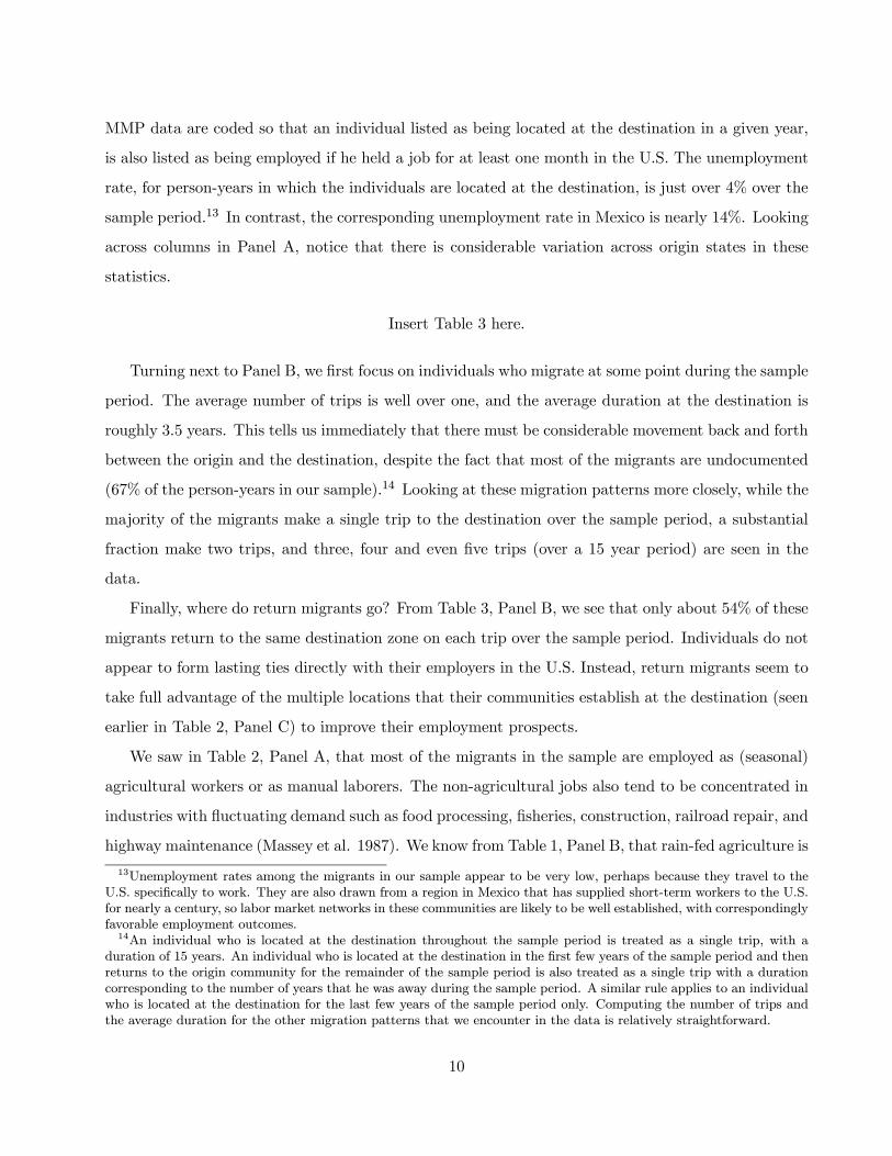
MMP data are coded so that an individual listed as being located at the destination in a given year,

is also listed as being employed if he held a job for at least one month in the U.S. The unemployment

rate, for person-years in which the individuals are located at the destination, is just over 4% over the

sample period.13 In contrast, the corresponding unemployment rate in Mexico is nearly 14%. Looking

across columns in Panel A, notice that there is considerable variation across origin states in these

statistics.

Insert Table 3 here.

Turning next to Panel B, we first focus on individuals who migrate at some point during the sample

period. The average number of trips is well over one, and the average duration at the destination is

roughly 3.5 years. This tells us immediately that there must be considerable movement back and forth

between the origin and the destination, despite the fact that most of the migrants are undocumented

(67% of the person-years in our sample).14 Looking at these migration patterns more closely, while the

majority of the migrants make a single trip to the destination over the sample period, a substantial

fraction make two trips, and three, four and even five trips (over a 15 year period) are seen in the

data.

Finally, where do return migrants go? From Table 3, Panel B, we see that only about 54% of these

migrants return to the same destination zone on each trip over the sample period. Individuals do not

appear to form lasting ties directly with their employers in the U.S. Instead, return migrants seem to

take full advantage of the multiple locations that their communities establish at the destination (seen

earlier in Table 2, Panel C) to improve their employment prospects.

We saw in Table 2, Panel A, that most of the migrants in the sample are employed as (seasonal)

agricultural workers or as manual laborers. The non-agricultural jobs also tend to be concentrated in

industries with fluctuating demand such as food processing, fisheries, construction, railroad repair, and

highway maintenance (Massey et al. 1987). We know from Table 1, Panel B, that rain-fed agriculture is

13Unemployment rates among the migrants in our sample appear to be very low, perhaps because they travel to theU.S. specifically to work. They are also drawn from a region in Mexico that has supplied short-term workers to the U.S.for nearly a century, so labor market networks in these communities are likely to be well established, with correspondinglyfavorable employment outcomes.14An individual who is located at the destination throughout the sample period is treated as a single trip, with a

duration of 15 years. An individual who is located at the destination in the first few years of the sample period and thenreturns to the origin community for the remainder of the sample period is also treated as a single trip with a durationcorresponding to the number of years that he was away during the sample period. A similar rule applies to an individualwho is located at the destination for the last few years of the sample period only. Computing the number of trips andthe average duration for the other migration patterns that we encounter in the data is relatively straightforward.

10

the major occupation at the origin, so weather fluctuations in Mexico will affect patterns of migration

as well. As a result, it is not at all surprising that migration patterns tend to be recurrent, with

individuals moving back and forth between Mexico and the U.S. as employment opportunities vary.

At the level of the community, this tells us that the number of migrants at the destination will be

changing over time, which is the principal source of variation that we exploit in the statistical analysis.

2.4 Job Search at the Destination

The literature in labor economics and sociology is replete with references to the importance of friends

and relatives in finding employment in the U.S. labor market, across occupational categories and ethnic

groups. For example, Rees (1966), in an early study set in Chicago, found that informal sources account

for about 50% of all hires in four white-collar occupations, and 80% of all hires in eight blue-collar

occupations. Similarly, Holzer (1988) found that friends and relatives were the two most frequently

used methods for finding employment in the 1981 panel of the National Longitudinal Survey of Youth

(NLSY). The same job search patterns have been obtained, with remarkable regularity, in study after

study of the U.S. labor market (Montgomery 1991, provides a summary).

Turning to migrant communities, we would expect the importance of social ties in the job search

process to be even stronger in these groups. Certainly, the received evidence overwhelmingly supports

the view that friends and relatives, and particularly those who belong to a common origin-community,

are the main source of information about jobs. Chavez (1992, p.136), for instance, tells the story of an

undocumented Mexican migrant: “Leonardo shared an apartment with seven other friends, all paisanos

from Sinaloa. Seven of the eight friends worked as gardeners. The first two friends had been in the

area for five years, and provided referrals for employers for each of the subsequent migrants, the last

of whom migrated two years earlier.” Over 70% of the undocumented Mexicans, and a slightly higher

proportion of the Central Americans, that Chavez interviewed in 1986 found work through referrals

from friends and relatives. Similar patterns have been found in contemporary studies of Salvadoran

immigrants (Menjivar 2000), Guatemalan immigrants (Hagan 1994), Chinese immigrants (Nee 1972,

Zhou 1992), as well as historically during the Great Black Migration (Gottlieb 1991, Grossman 1989,

Marks 1989).

Direct evidence from the MMP accords perfectly with this referral-based view of the job search

process. The household heads in our sample were asked how they obtained employment on their last

visit to the U.S. Turning to Table 4, we see that individual search (23%), relatives (35%), and friends

11

or paisanos (35%), account for the bulk of the jobs that were obtained. While not reported here, this

pattern of job-search is fairly even across the seven origin-states. If we include relatives, friends and

paisanos in the network, then it is clear that social ties play a significant role in obtaining employment

among the migrants in the sample.

Insert Table 4 here.

3 Networks in the Labor Market

My main objective in this section is to discuss conditions under which networks emerge in the labor

market, and to suggest ways in which these networks function. Some simple testable implications

of network effects emerge from this discussion, which also leads naturally to the discussion on the

identification of network effects that follows in Section 4. This section is based for the most part

on a model of labor market networks that was laid out in some detail in previous versions of the

paper (available from the author). Only one type of job is available to workers in that model: The

individual is either employed or unemployed. I will relax this assumption at the end of this section

since occupational choice plays such an important role in the empirical analysis.

3.1 Why do networks emerge?

To generate a role for social networks in the labor market we must begin with a positive level of

unemployment in equilibrium, which could for instance be generated by exogenous job turnover.

As noted in the previous section, the type of activities that our migrants are employed in, such as

agriculture and manual labor, are associated with frequent shifts in demand, so job turnover is likely

to be fairly high in this setting.

While job turnover will generate a positive level of unemployment, it does not by itself motivate

the emergence of a community-based network. For that, we must introduce some sort of information

problem in the labor market. Here one way to proceed would be to consider a model of costly search,

in which unemployed workers benefit from information about newly available jobs that they receive

from the employed members of their network (Carrington, Detragiache and Vishwanath 1996).

Alternatively, we could shift the information problem to the firm. Suppose that the firm is unable

to identify a freshly hired worker’s ability. If we make the usual assumption that the firm is unable

to specify a performance-contingent wage contract, then it would always prefer to hire a high ability

12

worker when a new position becomes available.15 The firm could choose to enlist the help of one of

its incumbent workers in this case, to recruit able workers from his network (as in Montgomery 1991).

The discussion that follows will restrict attention to this adverse selection model, since unobserved

ability plays such an important role in the identification of network effects.

3.2 How do networks function?

The simplest model of labor market networks with adverse selection treats the composition of the

network as exogenously given. Assuming that ability is positively correlated within a network, the

proportion of high ability workers will be higher on average in the incumbent high ability worker’s

network, as compared with the corresponding proportion in the market as a whole. At least some

firms will use referrals in this case, drawing randomly from the unemployed members of the incumbent

worker’s network, instead of drawing from the pool of (all) unemployed workers in the market.16

We could imagine instead that the incumbent worker has better information than the firm about

the ability of individuals in his network. This information asymmetry would also generate a role for

referrals, with the incumbent worker searching purposefully for high ability workers from his network.

We could relax the assumption that the composition of the network is exogenous in this case, although

this would be a more complicated model to solve. In addition, we would need to ensure that the

incumbent worker has an incentive to refer the most able individual from his network’s unemployment

pool to the firm (see Saloner 1985 for an analysis of this problem).

3.3 Who contributes to the network?

Focusing now on migrant networks, we would expect that it is the older migrants, those who have

been at the destination longer, who contribute disproportionately to the network.

If migrants arrive at the destination without a job, then employment levels will be increasing in

their duration at the destination, as they gradually escape from the unemployment pool (a detailed

15Piece-rate contracts are rarely used in the U.S. economy, and among the occupations that our migrants are employedin only agriculture is associated with the use of such incentive schemes. Data from the 1997-98 National AgriculturalWorkers Survey (UDL 2000) suggests that only 20% of agricultural workers are paid piece rates, with a slightly higherfigure (25%) for certain crops such as fruits, nuts, and vegetables. With about 50% of our migrants engaged in agriculture,these statistics tell us that only about 10% will face piece-rate contracts.16While the proportion of high ability workers may be higher on average in the incumbent high ability worker’s network,

what the firm really cares about is the proportion of high ability workers in the network’s unemployment pool. In aprevious version of the paper I showed that the proportion of high ability workers in the network’s unemployment poolalways remains at least as high as the corresponding proportion in the common unemployment pool in this set up, withat least some firms using referrals in equilibrium.

13

characterization of these employment dynamics was provided in an earlier version of the paper). Older

migrants provide more referrals in this case simply because they are more likely to be employed.

Further, among the employed migrants, older migrants will on average have been employed longer

by the firms that hired them. These workers will presumably have risen within the organizational

hierarchy, or accumulated a firm-specific reputation over time, and so have more to lose if they are

separated from their firms. The threat of separation, which helps ensure that the incumbent worker

only refers the most able available workers from his network, consequently has greater bite for the

older workers. This tells us in turn that the firm will be more likely to use referrals from such workers

in equilibrium.17 Older workers contribute more to the network in this case not necessarily because

they are more likely to be employed, but rather because they are employed longer on average.

3.4 Who benefits from the network?

Evidently it is individuals who would otherwise be unemployed who benefit most from the network.18

When firms draw randomly from the incumbent worker’s network, it is low ability workers in networks

with a large proportion of high ability workers that benefit most from the referrals.

When incumbent workers search purposefully for high ability recruits, only high ability workers will

be referred in equilibrium. Now it is individuals with unfavorable observed characteristics, competent

older migrants and women for instance, who will benefit most from the network.

3.5 Introducing multiple occupations

Up to this point we have assumed that there are only two labor market outcomes: The individual is

either employed or unemployed. However, all of the preceding discussion would still apply if multiple

occupations were available in the labor market.

For example, suppose that two occupations - higher paying non-agricultural jobs and lower paying

agricultural labor - are available. The network would now try and channel its members into the higher

paying non-agricultural jobs. Individuals are more likely to occupy these coveted positions as they gain

17While older workers may have had the opportunity to build a reputation with their firms, they are also more likelyto retire or, equivalently, to return to their origin communities, than workers who have just arrived at the destination.We would thus expect the threat of separation, and by extension the contribution to the network, to weaken beyond acertain age.18This need not be true if ability and network effects are complements, or if individuals could self-select into networks.

In that case, high ability workers could end up benefitting more from their network. The origin community exogenouslydetermines the boundaries of the network in this application, and the low-skill jobs that the migrants are employed inwould seem to rule out the complementarity assumption.

14

exposure at the destination, so the more established members of the network would also be better

positioned to provide non-agricultural referrals and channel individuals into preferred occupations.

Here again it would be individuals less likely to find non-agricultural jobs on their own, those who are

less educated for example, who would benefit most from the network.

Once we allow for multiple occupations, individuals might wait to receive a preferred job, and

larger networks could in principle be associated with lower levels of employment. However, as long

as switching jobs is sufficiently easy (which would seem to be the case for the kinds of jobs that our

migrants hold), a larger network should improve employment outcomes and channel individuals into

preferred occupations.

4 Identifying Network Effects

My objective in this section is to discuss the biases that arise with the estimation of network effects.

I make three assumptions to simplify the exposition, all of which will be relaxed later. First, there

are only two possible labor market outcomes: the individual is employed or unemployed. Second,

each individual works for two periods only. Third, he makes an irreversible location decision at the

beginning of his working life: he must choose between the “origin” (his Mexican community) and

the “destination” (the U.S.). This location decision will depend on the returns at the origin and the

destination over the next two periods, so our first task will be to describe these returns.

Begin with the employment outcome at the destination, which is in general determined by the

migrant’s ability, his duration at the destination, the network effect, and employment shocks at the

destination. Leaving aside the individual’s duration at the destination for the time being, the employ-

ment outcome for individual i in period t can be expressed as,

Pr(Eit = 1 | Xit = 1) = βXt−1 + ωi + Ct (1)

where Eit = 1 if the individual is employed, Eit = 0 otherwise. Xit = 1 if the individual chooses to

work at the destination, Xit = 0 otherwise. Xt−1 is the measure of migrants from his origin community

who moved to the destination in the previous period.19 Individuals work for two periods, and we take

19If we took the model laid out in the previous section seriously, then it is only employed individuals who can providereferrals, and so the relevant network size should be the measure of employed migrants at the destination. However, wewill see later that the network provides other support, such as financial assistance and housing, as well. So it would seemmore appropriate to use the measure of migrants, regardless of their employment status, as the size of the network. Thediscussion on identification would follow through with either network measure, and I will later verify that the estimatednetwork effects are robust to the method used to measure the network.

15

it that they only provide referrals in the second year of their working life, so a single cohort provides

referrals in each period. ωi is an idiosyncratic ability term which does not vary over time. Ct is an

employment shock that is common across individuals in the community but varies over time. Both

ωi and Ct are unobserved by the econometrician, and we will see below that it is these terms that

create problems for consistent estimation of the network effects, in the employment regression, by

being correlated with Xt−1.

The corresponding expression for the individual’s employment outcome in period t+1, Pr(Eit+1 |Xit+1 = 1) is obtained by replacing Xt−1 with Xt, and Ct with Ct+1. Xt, Ct+1 are unobserved by the

individual when he chooses his location at the beginning of period t, and we will see in a moment that

this will complicate his migration decision slightly.

Turning to the returns at the origin, we assume that the individual will be employed in the tradi-

tional activity (farming). Returns from farming depend on the weather, but not on the individual’s

ability.

Πit = Π(Zt) (2)

where Πit is the economic return at the origin and Zt is the rainfall in period t. We will see below

that we could introduce other determinants of Πit, including the individual’s ability, without affecting

the discussion that follows in any way. As before, the expression for the returns in period t+1, Πit+1,

is obtained by simply replacing Zt with Zt+1. When computing these returns, the individual must

account for the fact that Zt+1 is unobserved at the beginning of period t.

Normalizing so that the wage at the destination is unity, the individual will locate at the destination

if the expected return there over the next two periods, net of moving costs, is higher than the expected

return at home.20 The complication that arises immediately in this case is that the returns at the

destination in period t+1 depend on the measure of migrants that moves with the individual in period

t, Xt, so there is a strategic element to the individual’s location decision. In this case it is easy to

verify that a migration equilibrium for the cohort that starts working in period t is characterized by

a threshold ability ω, such that all individuals with ability greater than ω will choose to locate at the

destination.

20We could think of another decision rule in which the individual waits for a job opening at the destination (obtainedthrough his network), before migrating. But it is difficult to imagine that the individual would be able to get from hishome to the border, cross the border (most likely illegally), and then get to the job destination in time to fill the position.

16

Under what conditions will a unique interior solution for ω, in which a positive fraction of the

cohort locates at the destination in each period, be obtained? To begin with, we must consider the

coordination problem that could arise when a sufficiently large fraction of migrants is required to

sustain a viable network at the destination: everyone in the cohort could choose to remain at home in

that case. To rule out this possibility, we need to assume that a few of the highest ability individuals

in each cohort will always migrate, regardless of the (expected) size of the network at the destination.

Once migration has been initiated, we must then consider the possibility that the entire cohort

could “tip over” and locate at the destination (as in Carrington, Detragiache and Vishwanath’s (1996)

characterization of migration with endogenous moving costs). Starting with the highest ability migrant

in a cohort, each additional migrant will trade off the improvement in the performance of the network,

as a consequence of his own migration decision, with his lower ability (relative to the migrant before

him). An interior solution for the threshold ability ω will be obtained as long as the decline in ability

for each successive migrant sufficiently dominates the improvement in the performance of the network

as it expands.

Finally, we need to rule out “bumps” in the distribution, which could give rise to multiple equilibria.

A uniform ability distribution, together with the conditions described above, ensures that a unique

interior solution for the threshold ability ω will be obtained with each cohort.

Once we have characterized the migration equilibrium, each individual’s location decision is rela-

tively easy to describe.

Xit = 1 if ωi ≥ ω(Xt−1, Ct, Et(Ct+1), Zt, Et(Zt+1)) (3)

Xit = 0 otherwise

where Et(Ct+1) is the predicted employment shock in period t+ 1, and Et(Zt+1) is the predicted

rainfall at the origin in period t + 1. Et(Ct+1), Et(Zt+1) will in general be determined by the entire

history of employment shocks and rainfall shocks, up to period t. Favorable conditions at the destina-

tion can support lower ability migrants, so Xt−1, Ct, Et(Ct+1) will be negatively correlated with ω. In

contrast, only high ability individuals migrate when rains are plentiful at the origin, so Zt, Et(Zt+1)

will be positively correlated with ω.

Let the distribution of ability in any cohort be characterized by the function F . In that case, the

measure of migrants in period t is given by the expression:

17

Xt = 1− F (ω(Xt−1, Ct, Et(Ct+1), Zt, Et(Zt+1))). (4)

Working back one period, we can derive the corresponding expression for Xt−1:

Xt−1 = 1− F (ω(Xt−2, Ct−1, Et−1(Ct), Zt−1, Et−1(Zt))). (5)

We are now in a position to discuss the bias in the estimated network effects in equation (1) that

arises due to the unobserved ωi, Ct terms. Starting with the employment shock, we noted above that

favorable conditions at the destination are associated with a lower ability threshold ω. Thus high

Ct−1 in equation (5) is associated with a lower ω, and hence more migration Xt−1. If the employment

shocks are (positively) serially correlated, then Xt−1 will be positively correlated with Ct in equation

(1). This is a standard simultaneity problem that plagues the identification of social effects in general,

biasing the β estimate upward.

My solution to the simultaneity problem is to instrument for Xt−1 in the employment regression. A

valid instrument in this setting would determine Xt−1, while remaining uncorrelated with Ct or other

direct determinants of employment. A natural candidate that would appear to satisfy this condition,

from equation (5), is rainfall at the origin. Low Zt−1 reduces returns at the origin, and by extension

ω, which increases Xt−1. We would expect local rainfall shocks at the origin and employment shocks

at the destination to be uncorrelated since the origin communities in Mexico are located very far

from their U.S. destinations. Rainfall shocks at the origin and the destination, for each community,

are completely uncorrelated (the correlation coefficient is 0.01). Each community is also too small to

affect the level of employment at the destination through changes in its migration patterns.21 Zt−1

thus appears to be a valid instrument for Xt−1.

Changes in employment at the destination induce changes in location patterns, and we could in

principle have estimated a migration regression, corresponding to equation (1), with the migration

decision rather than the employment outcome as the dependent variable. The hypothesis in this case

21Rainfall shocks at the origin could still have a significant effect on labor supply at the destination if these shocksare correlated across the communities in each sending region. We also cannot rule out the possibility that even smallcommunities occupy a special niche in local markets at the destination, in which case changes in the size of the networkcould still affect access to employment. Note, however, that these general equilibrium effects would not spuriouslygenerate the pattern of rainfall coefficients that we saw in the reduced form employment regression (Figure 1). Forexample, an influx of migrants generated by low rainfall at the origin would lower employment at the destinationinitially, although these effects would dampen over time. This implies a positive coefficient on recent-past rainfall, witha weaker, but certainly not negative, distant-past rainfall effect.

18

would be that a larger network at the destination induces additional migration from the origin. The

problem with estimating this alternative regression is that while lagged rainfall Zt−1 may determine

the size of the network at the destination, it could also directly determine the individual’s migration

decision by affecting current employment outcomes at the origin (for example, if local institutions

that determine access to credit and other production inputs respond slowly to past rainfall shocks).

We will see later that lagged rainfall does in fact directly determine current employment outcomes at

the origin, and hence the individual’s migration decision, which rules out its use as an instrument for

the network in the alternative migration regression. Rainfall at the origin is a valid instrument for

Xt−1 in the employment regression precisely because we are restricting attention to activity at the

destination.

While the use of rainfall as a statistical instrument may solve the simultaneity problem in this

setting, we must still account for selectivity bias associated with the unobserved ability term ωi in

equation (1). E(ωi | Xit = 1) = φ(ω(Xt−1, Ct, Et(Ct+1), Zt, Et(Zt+1))), where φ is an increasing

function of the threshold ability ω. We noted earlier that an increase in Xt−1 improves conditions at

the destination, lowering ω. Thus, ωi will in general be negatively correlated with Xt−1. Intuitively,

more favorable conditions at the destination lower the (unobserved) quality of the migrants, biasing

β downwards. Instrumenting for Xt−1 does not solve the selection problem since ω is correlated with

Zt−1(through Xt−1).

My solution to the selection problem is to treat ωi as an individual fixed effect in the employment

regression. The implicit assumption here is that the individual’s ability does not vary over the sample

period. This seems to be reasonable, given the low-skill occupations that the individuals are engaged

in, both in Mexico and the U.S.

Before turning to the estimation results, I close this section with some extensions to the discussion

on identification:

1. Multiple work periods and return migration: Up to this point we have assumed that

each individual works for two periods, and makes an irreversible location decision at the beginning of

his working life. We will now proceed to relax both these assumptions.

The most obvious change in the employment regression, equation (1), is that multiple cohorts will

now provide referrals in each period. Following the discussion in Section 3, it is the older cohorts (who

have been at the destination longer) that will contribute more to the network.

19

While the size of a cohort continues to be determined by rainfall at the origin, each cohort no longer

responds exclusively to a single rainfall lag. For example, consider a network with two cohorts, Xt−1

and Xt−2. Zt−1 directly determines Xt−1, as we saw earlier.22 However, Zt−2 now also determines

Xt−1, through its effect on Xt−2 which in turn determines migration in period t − 1. By the samesort of argument, while Zt−2 directly determines Xt−2, Zt−1 also plays a role in determining the size

of this cohort by affecting the level of return migration in period t − 1. Although these cross-periodrainfall effects will complicate the interpretation of the rainfall coefficients in the first-stage migration

regressions reported later, notice that we continue to have a sufficient number of instruments for the

employment regression, with one rainfall lag for each cohort.

The preceding discussion can also be easily extended to the case, as in our data, where a fixed num-

ber of individuals in each community make location decisions over time. Migrants who have located

recently at the destination in any period t, correspond to the younger cohorts. Similarly, migrants

who are well established at the destination and better positioned to provide referrals, correspond to

the older cohorts. The rainfall instruments continue to apply in this case, with recent-past rainfall

directly determining the number of new migrants in the network, and distant-past rainfall determin-

ing the level of established migrants. We continue to have a sufficient number of instruments for the

employment regression, as above.

Individuals typically migrate to save up for a house, or to invest in a small business (Massey et

al. 1987). Once their target savings level is achieved they will return home, with the duration of

their stay depending on economic conditions at the origin and the destination, as discussed above.

Favorable conditions at the destination increase the speed at which the savings target will be achieved,

increasing the rate of return migration. Such attrition in the network would be most pronounced

among the established migrants, since recent arrivals must at least spend a few years at the destination

before they return. The estimated network effect, particularly the effect generated by the established

migrants, could thus be biased downward once we allow for return migration. The rainfall instruments

will, however, control for this additional source of bias as well since they are uncorrelated with the

employment shocks that induce the return migration.

2. The individual’s duration at the destination: Our view of the reduced form estimates

presented in Figure 1 is that low rainfall at the origin, four to six years ago, increases the measure

22The individual’s location decision, equation (3), is essentially unchanged, except that he makes this decision at eachpoint in his working life once we allow for return migration. While this decision continues to be forward looking, theworker must now account for the possibility that he could return to the origin in the future.

20

of established migrants today, improving the quality of the network and increasing employment rates

among its members. An alternative interpretation of this result, following the discussion in Section

3, is based on the idea that the probability of employment could be independently increasing in the

individual’s duration at the destination. The negative correlation between lagged rainfall and current

employment could then simply reflect compositional change in the network: Employment levels are

higher on average because there are more established migrants around.

One strategy to control for this confounding effect would be to estimate the employment regression

with fresh arrivals only - those migrants who arrived in period t or period t− 1. If such a migrant ismore likely to be employed if rainfall in his community was low in periods t − 4 to t − 6, then thiswould provide strong evidence that he is benefitting from the relatively large number of established

migrants, who arrived long before he did.23 As noted in Section 3, employment levels are likely to be

particularly low for the fresh arrivals, who would then benefit disproportionately from the network.

A strong implication of this view is that the estimated network effects should actually be larger for

the fresh arrivals, as compared with the effects obtained with the full sample.

3. Ability at the origin: We assumed that individual ability determines the employment outcome

at the destination but not the economic return at the origin. We could easily relax this assumption

and allow for an origin-specific ability ηi. Equation (2) is then rewritten as:

Πit = Π(Zt) + ηi.

The individual continues to make his location decision based on the returns at the origin and the des-

tination. The change here is that it is the ability differential ωi−ηi that determines which individualsmigrate. As Borjas (1987) points out, the nature of the selection bias is ambiguous in this case. If the

ability differential is systematically larger for low-ω individuals, then it is the low-ω individuals who

would be the first to migrate, and unobserved selectivity would bias the network effects upward rather

than downward as previously described. None of this matters, of course, as long as the individual

fixed effects account for the unobserved selectivity in the employment regression.24

4. Individual determinants of the employment outcome: Notice that equation (1) con-

23Once we allow for return migration, the individual’s duration at the destination will also respond to unobservedlabor market shocks. This test relies on the idea that fresh arrivals will stay at least a couple of years before they returnto the origin. We can thus restrict the sample to fresh migrants without biasing the estimated network effects.24Introducing other determinants of the economic returns at the origin in equation (2), which do not affect employment

at the destination, would not affect the estimation procedure in any way. All that we require is a single variable thatdetermines the level of migration, but is uncorrelated with employment shocks at the destination, to use as an instrumentfor the size of the network.

21

tained no individual determinants of the employment at the destination, apart from ability. Many of

these determinants, such as education, are time invariant and would be controlled for by the individual

fixed effects. Even if individual characteristics do change over time, omitting them from the employ-

ment regression creates no problems for consistent estimation of the network effects unless they are

correlated with the rainfall instrument. We saw in Figure 1 that employment depends on the number

of established migrants in the network, which is in turn determined by “distant-past” rainfall (more

than three years ago). Thus we need to rule out the possibility that distant-past rainfall shocks affect

current individual determinants of the employment outcome in this case.

One set of omitted characteristics that appear to be plausible in this environment are associated

with changes in the structure of the family. To explain a role for distant-past rainfall without network

effects we would have to argue that rainfall shocks bring about demographic change, such as a change

in marital status or the number of children, which translates into an increased incentive to seek

employment, but with a long lag. In the first place, it is difficult to suggest a plausible explanation

for such lags. Results not reported here also show that both marriage and fertility in the community,

unlike migration, are completely unaffected by rainfall at the origin.25

While individual ability might not change over time, the migrant’s reservation wage or search

intensity could respond to rainfall at the origin. For example, low rainfall could worsen the migrant’s

family’s economic condition at home, lowering his reservation wage and increasing his search intensity,

to the extent that he is tied financially to them.26 While this alternative explanation generates higher

employment among the migrants following a negative rainfall shock, it does not explain the long four-

year delay before employment starts to rise. We will later see that low rainfall lowers employment at

the origin immediately (in the same year), and we would expect information to flow fairly smoothly

within the community even across national borders, so this alternative explanation would predict an

employment response at the destination as early as the next year. Moreover, we will later see that

low rainfall leads to improved occupational outcomes - a shift into non-agricultural jobs - among the

migrants. A lowering of the reservation wage cannot explain this feature of the data as well.

5. Data problems: The discussion above dealt with problems for inference generated by selective

25Conditional on the stock of children or marital status in period t − 3, the number of children or marital status inperiod t is found to be completely uncorrelated with the recent-past rainfall shock (the average over t to t − 2 minusthe mean rainfall). Note that fixed effects are not included in these regressions since the demographic decisions areessentially irreversible.26Labor contractors might also tend to visit communities which have just received poor rains, to recruit cheap labor.

This effect is equivalent to an increase in the individual’s search intensity.

22

migration and unobserved determinants of labor market outcomes at the destination. We now turn

to problems with the data, which we will see could bias the estimated network effects as well. There

are essentially three data problems: measurement error in the network variable, recall bias due to

the retrospective nature of the data, and missing migrants on account of the fact that some of the

migrants might not have returned at Christmas time in the year of the survey. I will deal separately

with each of these potential sources of bias below.

Begin with the measurement error in the network variable. Remember that the econometrician’s

measure of the size of the network at the destination is based on a random sample of individuals drawn

from the community, so this variable will certainly be measured with error if we were to treat the

entire origin-community as the social unit.27 The rainfall instrument avoids measurement error as well

in this case, since rainfall shocks at the origin determine the level of migration in the community, but

provide no information about deviations from the true level of migration. Note that the measurement

error attenuates the network effect down towards zero.

Next, consider the missing migrants. The surveys were conducted around Christmas time in each

community, which is when the migrants typically return home to visit their families. But it is always

possible that some migrants might not have returned in the survey year. To understand the bias

that could arise in this case, return to the simple set up in equation (1), where migrants remain

at the destination for two periods only and provide referrals in the second period, but now assume

that there is a single cohort that works for many periods and that return migration and multiple

trips are possible. Further, a fixed fraction θ of the established migrants remain at the destination

at Christmas time, and so will be missed by the survey, which to begin with occurs every period.

Ignoring the selectivity issue and the simultaneity bias that we discussed above, equation (1) can be

rewritten as:

Pr(Eit = 1 | Xit = 1) = βXt−1 + [βθXt−1 + Ct] , (6)

where we now assume for simplicity that Xt−1 and Ct are orthogonal. Xt−1 is the observed size of

the network, and θXt−1 is the unobserved component of the network. It is straightforward to derive an

expression for the network effect in this case: plimβ = β/1− θ. As the unobserved component of the

network (θ) grows, the upward bias in the network effect grows with it. In general, if the established

27Classical measurement error, possibly in a more severe form, would also arise if each individual’s network consistedof a limited number of partners drawn randomly from the community.

23

migrants are less likely to return at Christmas, then the relatively large contribution to the network

that we later attribute to this group would be biased upward.

However, things are not as bad as they might seem. The survey is not conducted every year,

but only at one point in time, which we will refer to as period T . There is a single group of θXT−1

individuals, who happen to have migrated in period T − 1, and who happen to have stayed awaywhen the survey was conducted. Only those individuals will be missing in all the sample years prior

to period T . Since individuals are independently moving back and forth over time, it is very unlikely

that all θXT−1 of those individuals would have been together at the destination in any year other

than period T . Individuals remain at the destination for a few years, so we would expect to see some

persistence. But this should soon disappear, and thereafter only a small (random) fraction of the

θXT−1 individuals will be together at the destination in any given year.

The pattern over time that we have just described should hold not only for the missing group, but

also for the (1−θ)XT−1 migrants who are observed at the destination in the survey year. To empirically

verify the preceding argument, we focus on the location patterns over time of those individuals who

were established migrants at the destination in the survey year. Figure 2 plots the proportion of those

individuals who continue to be established migrants as we move back in time from the survey year

(with the corresponding 95 percent confidence interval band). As expected, there is a sharp initial

decline in this proportion, followed by a flattening out thereafter.28

Insert Figure 2 here.

The discussion above and Figure 2 tells us that the upward bias due to the missing migrants could

be significant in the survey year, and the years just prior to that year. But relatively clean estimates

of the network effects should be obtained if those years are discarded from the sample. Following this

discussion we will experiment with different sample periods in the empirical analysis.

Finally, we turn to recall bias. The regression analysis uses information on where the individual

was located in each year, whether or not he was employed, and the broad occupational category that

he was hired in if he was working. This is fairly basic information and we would expect accurate

responses, going back many years before the survey year. In the event that there are any errors,

this is only cause for concern with our instrumental variable procedure if the errors are systematic.

28Figure 1 and Figure 2 utilize the Epanechnikov kernel function. Pointwise confidence intervals in Figure 2 arecomputed using a method suggested by Hardle (1990).

24

For example, if individuals systematically report that they are at home when they are in fact at the

destination, then the network size will be biased downward and the discussion above tells us that the

estimated network effects will be biased upward. If the recall error goes in the opposite direction,

then the bias in the estimated network effects goes in the opposite direction as well. We would expect

such errors to grow more frequent as we move further back in time, and so one way to check for such

recall bias would be to experiment with longer sample lengths (20 years prior to the survey year in

each community) to verify the robustness of the estimated network effects.

6. Occupation as the outcome of interest: Up to this point we have assumed that there are

only two labor market outcomes: The individual is either employed or unemployed. Once we allow for

multiple occupations, we would also expect the network to move its members into preferred jobs. In

this application, two broad classes of occupations are available to the migrants: agricultural labor and

higher paying non-agricultural jobs.29 To disentangle the effect of the network on occupational choice

from its effect on employment, I will now restrict attention to individuals who are always employed in

the years in which they locate at the destination (Ei = 1). Each of those individuals should be more

likely to hold a non-agricultural job in years in which his network is larger. The occupation regression

can then be specified as follows:

Pr(Nit = 1 | Ei = 1,Xit = 1) = γXt−1 + ωi +Dt (7)

where Nit = 1 if the individual holds a non-agricultural job, Nit = 0 if he has an agricultural job.

Dt is an unobserved labor market shock, which reflects the demand for non-agricultural labor relative

to agricultural labor.

As before, we control for the unobserved ωi term with individual fixed effects. Xt−1 is correlated

with Dt for two reasons: First, higher Dt implies that more high-wage non-agricultural jobs are

available, which induces additional migration and biases the γ estimate upward. Second, greater access

to non-agricultural jobs increases the speed at which migrants achieve their target savings, hastening

return migration and biasing γ in the opposite direction. As with the employment regression, the

rainfall instrument continues to be orthogonal to Dt, providing us with unbiased estimates of the

effect of the network on occupation choice.

29The MMP data set lists 81 occupations, which are further classified into broader categories, one of which is agricul-tural jobs.

25

5 Empirical Analysis: Employment at the Destination

The network is seen to influence two labor market outcomes in this paper: The migrant’s employment

outcome and, conditional on being employed, the type of job that is obtained. We begin the empirical

analysis in this section with employment as the outcome of interest. Subsequently we turn to the

occupation as the dependent variable in Section 6.

The individual’s employment is a binary variable, which takes on a value of one if he is employed,

zero otherwise. A fixed number of individuals (typically 200) were interviewed in each community,

so our measure of the size of the network will be the proportion of the sample that is located at the

destination at each point in time.

The basic employment regression uses rainfall at the origin as an instrument for the size of the

network. We will also consider a reduced-form specification with lagged rainfall as regressors. This

section begins with the reduced-form employment regressions in Sections 5.1 and 5.2. Subsequently we

turn to the instrumental variable (IV) estimates in Section 5.3, before concluding with a discussion on

the robustness of our results in Section 5.4. The Linear Probability model, with fixed effects and year

dummies, is utilized for all the employment regressions that we estimate in this paper.30 Following

the suggestion of a referee, women who account for 3% of the migrants are dropped from most of the

regressions that I report in this paper. We will later see in Table 9 that the estimated network effects

actually increase when the women are included in the sample, so the results that I report are most

likely conservative estimates of the network effects.

5.1 Reduced Form Regressions: Fine Partition of Rainfall Lags

We begin in Table 5 with the reduced-form specification of the model, regressing employment on

lagged annual rainfall. We know from Section 4 that low rainfall at the origin increases migration to

the destination, which in turn increases employment among the migrants through the network effect.

This tells us that employment should be negatively correlated with rainfall. Turning to Column 1,

the first empirical result of this section is that employment at the destination is negatively correlated

with lagged rainfall at the origin, as expected. Further, it is the longer rainfall lags that seem to have

30While the sample period covers 15 years prior to the survey year in most communities, the data span a much longertime period (1973-1995) since our communities were surveyed at different points over the 1982-1995 period. We use lessthan 15 years for the analysis in the very earliest communities because the rainfall series does not go that far back.

26

a greater effect on employment.31

Insert Table 5 here.

Why should rainfall at home, more than three years ago, affect the individual’s employment out-

come in the U.S. today? Recall from Section 4 that long rainfall lags directly determine the number

of established migrants in the network today, and we know from Section 3 that the older cohorts are

better positioned to provide referrals in the network. Our interpretation of this reduced form result,

which we will subsequently verify, is that long rainfall lags have a stronger effect on employment out-

comes at the destination because they determine the number of established migrants in the network,

at each point in time.

The basic idea behind the instrumental variable procedure in this paper is that low rainfall at

the origin should adversely affect economic returns there, increasing migration to the destination.

One convenient measure of the returns at the origin, which is available to the econometrician, is

the individual’s employment outcome. I consequently replace employment at the destination with

employment at the origin as the dependent variable in Column 2. Restricting attention to person-

years in which the individual is located in the origin community, we see as expected that employment is

now increasing in lagged rainfall.32 Moreover, it is the current and recent lags that affect employment

the most, suggesting that migration should respond quickly to negative rainfall shocks at the origin.

This useful result directly motivates the first stage regressions that we will examine below.

5.2 Reduced Form and First-Stage Regressions: Coarse Partition of Rainfall Lags

Roughly 12% of our observations (where each observation is a person-year) are located at the destina-

tion over the sample period. With 200 individuals in a community, this leaves us with approximately

24 migrants, spread over many years of exposure, at each point in time. Clearly there are too few

migrants to estimate network effects separately for each level of exposure. My approach instead is

to partition the network into new migrants and established migrants. Since lagged rainfall helps de-

termine the pattern of migration, the estimates in Table 5 provide us with a convenient cut-off to

31The coefficient on lagged rainfall declines sharply after t−6, which explains my choice of lag-length in these reduced-form regressions.32We would also expect that employment in communities with higher levels of irrigation should respond less to rainfall

shocks. Regression results not reported here reveal that this is indeed the case. Note that irrigation levels are potentiallyendogenous and could respond to employment shocks at the origin, as well as at the destination (through remittancesor past migration spells). Thus we only use uninteracted rainfall as instruments in the employment regressions that wereport later, although the IV estimates of the network effects are very similar with and without the irrigation-rainfallinteraction terms.

27

separate these categories. Recall that rainfall was insignificant for the first three lags (t to t− 2), andsignificant and stable thereafter (t− 3 to t− 6).

Before verifying the link between rainfall and migration, which is essentially the first-stage of the

instrumental variable (IV) regression, I first proceed to replicate the reduced-form regressions that

we studied in Table 5, with this coarse partition of the rainfall lags. Recent-past rainfall is measured

as the average rainfall over the periods t to t − 2, while distant-past rainfall is measured as thecorresponding average over t− 3 to t− 6. We are implicitly restricting the coefficients on recent-pastrainfall t to t− 2 to be the same, with a corresponding restriction on the coefficients for distant-pastrainfall t − 3 to t − 6, in this alternative specification of the reduced form employment regression.

As expected, employment responds strongly in Table 6, Column 1, to distant-past rainfall, but is

unaffected by recent-past rainfall.33 Moreover, the coefficient on distant-past rainfall is roughly four

times the coefficient on the t − 3 to t − 6 lags in Table 5, which is what we would expect since thecoefficients were fairly stable across the four years.34

Table 6, Column 2 repeats the exercise that we just described, with an alternative cut-off for the

recent migrants at t − 3, instead of t − 2. While the coefficient on distant-past rainfall (the averageover t−4 to t−6) is now slightly smaller than it was in Column 1, the basic patterns that we observedearlier are unchanged.

Insert Table 6 here.

As noted in Section 4, one simple strategy to disentangle the network effect from the individual

exposure effect is to restrict attention to fresh arrivals. Restricting attention to those migrants who

arrived in the current year or the previous year in Column 3, we see that the basic pattern observed in

Columns 1-2 is unchanged. The coefficient on the established migrants actually increases substantially,

which is consistent with the view that the newcomers should be more dependent on the network.

33Figure 1 is obtained by differencing out the fixed effects and the year dummies from a first stage parametric regressionthat matches the specification in Column 1, except that recent-past rainfall is not included as a regressor. The linearity inFigure 1 tells us that the first stage is flexible enough to capture the basic features of the employment-rainfall relationship.While we control for clustered residuals in each community-year when computing the standard errors in this paper, wewould need to allow for clustering at a more aggregate state-year level if rainfall shocks were correlated across neighboringcommunities. Although the within-state coefficient of variation is slightly smaller than the between-state coefficient (0.42versus 0.52), these statistics are quite comparable, suggesting little spatial correlation in the rainfall shocks. Further,standard errors that allow for state-year clustering are almost identical to what we report in this paper.34I also experimented with the conditional (fixed effects) logit model to check the robustness of these results. While the

point estimates for the logit and the linear probability model are not directly comparable, the coefficient on distant-pastrainfall continues to be negative and significant at the 5 percent level, while the coefficient on recent-past rainfall isinsignificant.

28

Most of the employment regressions in this paper, including those reported up to this point, include

individual fixed effects to control for unobserved selectivity in the migration decision. This implies

that we are identified from the 5% of person-years at the destination that apply to migrants who report

both employment as well as unemployment over the sample period. This is not a problem if we are

only interested in identifying the presence of the network effects, or in studying the broad qualitative

nature of these effects (such as the relative importance of the established migrants in the network).

However, the magnitude of the estimated network effects must now be interpreted with care.

While I mentioned in Section 3 that individuals who are less likely to be employed will benefit

more from the network, I did not account for this potential variation across individuals later in the

estimation section. Since most of our migrants are always employed, those individuals who report both

employment and unemployment over the sample period are by definition those who would benefit most

from the network. Thus while our fixed effects estimates would correctly measure the network effects

for that vulnerable group of individuals, they could substantially overestimate the average effects for

the community as a whole.35

One strategy to avoid this problem would be to replace individual fixed effects with community

dummies in the employment regression. If we were to take the expectation of the employment outcome,

across all the individuals at the destination in each community-year, the dependent variable in the

equivalent community level regression would then be the proportion of migrants employed in each

year. Network effects in the regression with community dummies are thus effectively estimated from

changes in community-level employment over time. The reduced form employment regression with

community dummies is presented in Column 4 of Table 6. The point estimates are remarkably similar

to what we obtained earlier in Column 1, increasing our confidence in the robustness of these results.

Finally, I complete the replication of the reduced-form results, with the coarse partition of the

rainfall lags, by studying employment outcomes at the origin in Column 5. Employment is increasing

in lagged rainfall, particularly recent-past rainfall, just as we saw in Column 2 of Table 5, which leads

us quite naturally to the migration regressions that follow.

Turning to the first stage of the IV regression in Columns 6-7, we see that the numerical strength of

the new (established) migrants is negatively correlated with recent-past (distant-past) rainfall, support-

35Goldin and Rouse (2000) must deal with the same problem in their study of gender discrimination, where they areidentified from 6% of the individuals in the sample with individual fixed effects. While Goldin and Rouse argue that those6% are drawn randomly from the full sample, their approach does not appear to be plausible in our setting; individualswho report spells of unemployment over the sample period are very likely to have lower than average ability, or observedcharacteristics that signal low ability.

29

ing our interpretation of the reduced-form estimates.36 Notice also that the coefficient on distant-past

rainfall is positively correlated with the numerical strength of the new migrants. We saw above that

low distant-past rainfall reduces current employment levels at the origin, which would increase new

migration. Low distant-past rainfall also improves the quality of the network by increasing the number

of established migrants, which would in turn induce additional new migration. However, since there is

a fixed number of individuals in each community, low distant-past rainfall also reduces the number of

potential new migrants by increasing the number of established migrants. The positive coefficient on

distant-past rainfall in Column 6 suggests that the third effect must dominate. Note that the coeffi-

cient on recent-past rainfall in Column 7 is insignificant. While recent-past rainfall could in principle

induce return migration, this does not seem to be the case with our data.

5.3 OLS and Instrumental Variable Regressions

We now proceed to directly verify the relationship between the network and employment at the desti-

nation. Starting with a preliminary OLS regression in Column 1 of Table 7, we see that the individual’s

employment outcome depends strongly on the numerical strength of the established migrants, but is

unaffected by the new migrants. While the OLS results are consistent with our interpretation of the

reduced-form estimates, we have yet to account for simultaneity bias or measurement error in the

network variables. While individual fixed effects account for selective migration, we must turn to the

IV regressions to obtain consistent estimates of the network effects. Looking at the IV estimates, in

Column 2 of Table 7, new migrants continue to play a negligible role, while the established migrants

are even more influential then they were in the OLS regression reported in Column 1. Rainfall shocks

at the origin are clearly uncorrelated with unobserved employment shocks at the destination. Rainfall

is also a good instrument for the strength of the network; the rainfall coefficients in Columns 6-7 of

Table 6 are statistically significant and the F-statistics are comfortably above the critical value at the

5% significance level in both regressions. We should thus be fairly confident about the consistency

of the IV estimates. The discrepancy between the OLS and the IV estimates might arise because

favorable conditions at the destination induce return migration among the established migrants who

36The regression in Column 7 corresponds to the nonparametric migration regression in Figure 1, except that recent-past rainfall is included as an additional regressor to allow for return migration, and that individual fixed effects ratherthan community dummies are included. Note that the additive separability in all the reduced form and first stageregressions in the paper is appropriate in this case. For example, this is appropriate in Column 7 because recent-pastrainfall changes the number of established migrants in the network at the margin, by shifting the ability threshold fromone period to the next, instead of changing the general probability that any established migrant would return (in whichcase interaction terms would be required.

30

have achieved their savings target, biasing the network effects attributable to this group of migrants

downward. Measurement error in the network variable could also have attenuated the OLS estimates

in Column 1.37

Next, I consider an alternative cut-off for new migrants at t − 3, so the established migrants aredefined as those individuals who have been at the destination for four years or longer. The IV estimates

with this alternative cut-off in Column 3 are almost identical to what we observed in Column 2.

Insert Table 7 here.

Up to this point in the discussion we have not accounted for the possibility that employment rates

could be independently increasing with the individual’s exposure at the destination (on the current

trip). Restricting attention to fresh arrivals in Column 4, the estimated network effects are actually

substantially larger than the network effects that we obtained with the full sample. This is exactly

what we would expect, since the newcomers should be more dependent on the network for referrals.

The remaining regressions in Table 7 verify the robustness of the IV estimates. Column 5 begins by

replacing individual fixed effects with community dummies, without changing the estimated network

effects at all. Subsequently we replace the proportion of migrants by the proportion of employed

migrants as the measure of the network variable in Column 6. We will later see that the network

provides many services to its members: It provides financial support and housing assistance, in addition

to job referrals, which is why the network was specified to be the proportion of migrants at the

destination in Section 4, and in the empirical analysis this far. If we were to take the model laid

out in Section 3 seriously, however, the correct measure of the network is the proportion of employed

migrants at the destination. The results in Column 6 tell us that the estimated network effects are

now slightly smaller, but the basic qualitative patterns that we have seen throughout Table 7 remain

unchanged.

Finally, we account for the observation in Table 2 that each community sets up multiple centers

- typically two to three large ones - in the U.S. The appropriate measure of the network might then

be the number of paisanos in the state that the migrant is located in, rather than the corresponding

37Another explanation for the difference between the OLS and the IV estimates is that low ability individuals are moreresponsive to rainfall shocks at the destination. In that case, the OLS estimates will apply to the migrant with averageability, while the IV estimates will apply to a migrant with lower than average ability, and we know that low-abilityindividuals benefit more from the network. I checked to see whether individuals with observed characteristics that signallow ability (women, older men, less educated men) are more likely to migrate when rainfall in the origin community islow, but was unable to uncover any systematic pattern in the location decisions.

31

statistic for the U.S. as a whole. Estimates with this alternative measure of the network, which also

include a full set of state dummies in the employment regression, are reported in Table 7, Column 7.

Once more we see that the basic patterns that we saw earlier continue to be obtained.

The communities in our sample vary in size, and are drawn from both rural and urban areas.

While the results that we have reported do not distinguish between communities with different char-

acteristics, we would expect small, rural, communities (ranchos) to be more cohesive, and therefore

better positioned to support their members at the destination. Dropping these communities from the

sample in Table 7, Column 8, we see that the network effect does decline, and is no longer significant

at the 5 percent level. Nevertheless, the basic pattern, with the established migrants contributing

disproportionately to the network, continues to be obtained.

5.4 Employment Regressions - Additional Tests

We saw in the previous section that network effects appear to depend on community characteristics.

We would expect network effects to depend on individual characteristics as well; the discussion in

Section 3 tells us that individuals independently less likely to be employed would benefit most from

the network. We have already seen some evidence that is consistent with this prediction. Recall that

network effects are considerably larger for recent arrivals in Table 7, and we would expect newcomers

to the labor market to have higher unemployment rates in general. We will pursue this idea further, in

the discussion that follows, using other individual characteristics that would a priori seem to determine

unemployment levels.

Table 8 partitions the sample, which now includes both men and women, into employed and

unemployed migrants. The person-year is the unit of observation in this Table. Row 1 presents the

proportion of males among the employed and the unemployed observations. Very few of the migrants

are female, and we see in Column 2 that female account for only 2% of the employed person-years at

the destination. However, females account for 28% of the observations that list unemployed status.

Clearly, females account for a large proportion of the unemployed person-years in the sample.

Insert Table 8 here.

Continuing with the comparison between the employed and the unemployed person-years, we see

in Row 2 that the unemployed are more than 13 years older than the employed. These result are not

surprising. Both women and older men have observable characteristics that signal lower ability to

32

perform the sort of physical jobs that the migrants engage in. The network can play a very useful role

in this case, since those members of the network who are providing referrals have better information

than the market about the true ability of these workers.

Turning to schooling in Row 3, we find that education levels are higher among the unemployed.

We will see later that higher schooling appears to provide greater access to non-agricultural jobs. But

those with education might also be unsuited for the more physical agricultural jobs, so the net effect

of education on employment could go either way.

Table 9 tests the predictions generated by the preceding discussion. In general, we would expect

individuals with characteristics associated with higher unemployment levels in Table 8 to benefit more

from the network. The presumption in this case is that the network cannot overcome the individual’s

inherent limitations in the labor market. Those individuals who would independently be less likely to

be employed will benefit the most from the network, but they will continue to display lower employment

levels in equilibrium. Column 1 includes both men and women in the sample, and we see as expected

that the network effects increase substantially as compared with the corresponding estimates for men

only in Table 7, Column 2. Subsequently we return to the standard specification with men only, but

restrict attention to men less than 55 years old in Table 9, Column 2 and men less than 45 years old

in Column 3. The network effects do decline, as they should, and while these results are not reported

here, they decline even further when the age ceiling is lowered to 35 years. But the network response

to age is not as dramatic as it was for the women.

Insert Table 9 here.

Table 9, Column 4 continues with this exercise, restricting attention to individuals with less than

10 years of education. A natural cut-off separating more and less educated migrants would be high

school completion (12 years of education). But only 5% of the migrants achieved this level of schooling,

so I report estimates with a less stringent 10 year cut-off, which leaves us with 90% of the full sample.

The estimated network effects in Column 4 are almost exactly what we observed earlier in Table 7,

Column 2. I experimented with alternative cut offs from nine to 12 years, without changing this result.

The empirical analysis up to this point has checked the robustness of the estimated network effects

to alternative measures of the network, community characteristics, and individual characteristics. But

we have yet to account for the potential data problems - recall bias and missing migrants - that we

discussed in Section 4. A simple test to rule out recall bias would be to verify that the estimated

33

network effects are robust to an increase in the sample length, say up to 20 years before the survey

year. For the bias associated with the missing migrants, one solution would be to drop the survey

year and the years just prior to the survey year from the sample, since we saw in Figure 2 that the

bias falls very sharply over time.

We begin in Table 9, Column 5 by increasing the sample length to 20 years preceding the survey

year, in each community. The network effects are very similar to what we obtained with the 15-year

sample length in Table 7, Column 2. Subsequently we return to 15 years prior to the survey year as

the earliest period in the sample, but discard the survey year (T ) and the year before it (T − 1) inColumn 6. The network effects now decline, and this trend continues when we discard an additional

year (T − 2) in Column 7. But notice that the network effects stabilize from Column 7 to Column 8 -

discarding year T −3 has little effect on the network estimates. While not reported here, this stabilityis maintained when we discard one more year, T − 4; the point estimate declines only slightly to 0.9.

6 Empirical Analysis: Occupation at the Destination

The empirical analysis concludes by studying the role of the network in shifting its members into

preferred non-agricultural jobs. We begin by comparing the earnings and the characteristics of agri-

cultural and non-agricultural workers in Section 6.1. Subsequently we compare the community ties

and the assistance received by these workers in Section 6.2. Non-agricultural workers earn more and

are more likely to receive assistance from the community, so there is some prima facie evidence that

the network is channelling its members into non-agricultural jobs. But as we discussed in the Intro-

duction, other explanations for these patterns in the data are also available. Consequently, Section 6.3

and Section 6.4 report more robust results from occupation regressions, with individual fixed effects

and rainfall as the instrument for the network, where we see that the same individual is more likely

to hold a non-agricultural job when his network is exogenously larger.

6.1 Occupational Choice - Labor Market Outcomes and Individual Characteristics

The MMP data set provides very limited information at each point in time over the individual’s

working life; where he was located, whether or not he was employed, and the kind of job he had if he

was employed. However, much richer information is available about the migrant’s earnings and the

assistance that he received from the community on his last trip to the U.S. We will use this information

34

from the last trip to compare agricultural and non-agricultural workers in the discussion that follows.38

Table 10, Panel A, describes the wages and the duration of employment for the two types of

workers. Since communities were surveyed at different points in time, and the individuals in each

community would also have made their last trip in different years, the last trip of all the migrants

in the sample ranges over many years. The reported nominal wages must therefore be normalized

to account for this variation over time: Row 1 reports the ratio of the hourly wage to the minimum

wage, while Row 2 reports the real wage in 2001 dollars. Agricultural workers earn about 20% more

than the minimum wage ($6.92 per hour) while non-agricultural workers earn about 40% more than

the minimum wage ($8.06 per hour). All of these earnings differentials in Table 10 are statistically

significant at the 5 percent level, and factoring in the number of hours worked in the year by each

type of worker, the non-agricultural workers earn $3,300 more than the agricultural workers, which is

as much as 40% more than average agricultural earnings.39

Table 10, Panel A, also reports the average job durations for the two types of workers. Agricultural

labor tends to be seasonal, but the work is intense during the season. Not surprisingly, the agricultural

workers work longer hours per week, but for less than six months in the year; these differences between

agricultural and non-agricultural workers are once more statistically significant at the 5 percent level.

Insert Table 10 here.

The skills required for agricultural and non-agricultural work are not the same, and we saw above

that the earnings from these two types of occupations differ significantly. We would thus expect the

characteristics of workers in agricultural and non-agricultural occupations to differ as well. As in Table

6, we compare the two types of workers along the sex, age, and education dimensions in Table 10,

Panel B.

Starting with sex in Row 1, we see that women are slightly more likely to be in non-agricultural

jobs (3% versus 1%). Looking at the age in Row 2, we see that non-agricultural workers are about

four years younger than agricultural workers. But these differences are small, compared with what

we saw earlier in Table 6. Recall that women accounted for 28% of the unemployed person-years, and

38For those cases in which the migrant held more than one job on the last trip, the MMP lists the job with the longestduration as his occupation.39We will see below that non-agricultural workers are younger and better educated than agricultural workers, and

hence may be more able. However, the income differential for agricultural and non-agricultural workers does not changeappreciably when I control for individual characteristics such as sex, age, education, and the migrant’s primary occupationat the origin; the income differential only declines from 3, 300 to 3, 200. The migrant clearly benefits a great deal bygaining access to a non-agricultural job.

35

that the age difference between the employed and the unemployed was as high as 13 years. We thus

would not expect to see sex or age have the same impact on the network effects as they did in the

employment regressions in Table 9. Moving down to schooling in Table 10, Panel B, we now see that

individuals holding non-agricultural jobs have substantially higher education. The implication in this

case is that the network should help less educated individuals obtain these coveted non-agricultural

jobs.40

6.2 Occupational Choice and Community Support

We saw above that non-agricultural workers earn more and have different characteristics, as compared

with the agricultural workers. In the discussion that follows we will see whether the community treats

these two types of workers differently as well.

Table 11, Panel A, reports the migrant’s contacts with relatives and paisanos at the destination. A

large proportion of workers had contact with the community on their last trip, with both agricultural

and non-agricultural workers reporting similar levels of contact.

Insert Table 11 here.

While the focus of this paper is on direct assistance in finding jobs, the MMP data also provide

information about financial assistance and housing assistance received by the migrants. Table 11,

Panel B, reports financial assistance received from the community. Possible sources of assistance

are relatives, friends or paisanos, employer, and others. The important difference between the two

types of workers is in the help from relatives: 30% of the non-agricultural workers versus 20% of

the agricultural workers report assistance from their relatives. Pooling together relatives, friends and

paisanos, we compute the proportion of workers who report financial assistance from the community

at the bottom of Panel B: 37% of agricultural workers versus 45% of non-agricultural workers (these

differences are significant at the 5 percent level).

Subsequently we turn to housing assistance in Panel C. The same sources of assistance listed in

Panel B above appear here as well. As with financial assistance, a much greater proportion of non-

agricultural workers (61% versus 37%) report housing assistance from their relatives. Such assistance

40As with the employment regression, the presumption here is that the network cannot overcome the individual’sintrinsic limitations. Those individuals who are less likely to hold non-agricultural jobs to begin with will benefit morefrom the network, but will nevertheless remain less likely to hold those jobs in equilibrium.

36

appears to substitute for the absence of employer-provided housing among the workers: 31% of agri-

cultural workers versus 6% of non-agricultural workers received housing from their employers. Pooling

relatives, friends, and paisanos as before, 61% of agricultural workers versus 88% of non-agricultural

workers report housing assistance from the community (these differences are once more statistically

significant).

Finally, we turn to job search in Panel D. We have already seen in Table 4 that a substantial

proportion of the migrants in the sample received job referrals from their community. Here too,

relatives, friends, and paisanos are the dominant source of information about jobs, for both agricultural

and non-agricultural workers. Pooling all these sources of community assistance, non-agricultural

workers are once again significantly more likely to receive job referrals from their community (74%

versus 64%).

6.3 Reduced Form, OLS, and Instrumental Variable Regressions

We have seen that non-agricultural workers earn significantly more than agricultural workers. We

have also seen that non-agricultural workers are significantly more likely to receive financial assistance,

housing assistance, and job referrals from the community. While this evidence does suggest that the

network is actively channelling its members into preferred non-agricultural jobs, other explanations

are also available. For example, we saw in Table 10 that non-agricultural workers are younger and

better educated on average. If such individuals were favored by the network for other reasons, then

a spurious correlation between the network and occupational choice could be obtained. Alternatively,

the information problems that generate a need for job referrals might be more severe in the non-

agricultural jobs.41 It also appears that agricultural workers are more likely to receive housing from

their employers, which tells us that the demand for housing assistance from the community may be

greater among the non-agricultural workers. The network might be more active in the non-agricultural

occupations simply because there is a greater demand for its services from individuals who happen to

be employed in those occupations.

The test that we propose to establish an active role for the network in moving its members into

non-agricultural jobs is to see whether the same individual is more likely to hold a non-agricultural job

in years in which his network at the destination is exogenously larger. This test is easily implemented

41As noted in Section 3, piece-rate contracts are rarely used in the U.S. economy, one of the few exceptions being theagricultural sector. Once a farm can use a piece-rate contract, it is immediately less dependent on job referrals.

37

by replacing employment with the occupational outcome, and by including individual fixed effects and

using rainfall as an instrument for network size in the occupation regression. As discussed in Section 3,

we run this regression with the 95% of the migrants who are employed in all years that they locate at

the destination, allowing us to isolate the role of the network in affecting occupational choice. Unlike

the employment regressions, in which there was very little variation in the dependent variable, we saw

in Table 2 that non-agricultural jobs account for 51% of the person-years at the destination. Including

individual fixed effects is also no longer a problem, since as many as 18% of the always employed

migrants change their occupation over the sample period.

We begin in Table 12, Column 1, with the reduced form occupation regression. The dependent

variable equals one if the individual has a non-agricultural job, zero if he is an agricultural laborer.

Recent-past rainfall and distant-past rainfall are included as regressors in this fixed effects regression,

which is restricted to male migrants as before. As with the employment regression, the coefficient

on recent-past rainfall is insignificant, while the coefficient on distant-past rainfall is negative and

significant. We already know, from the first stage regressions reported earlier, that low distant-past

rainfall translates into a larger number of established migrants at the destination. Our interpretation of

this reduced form result is that an exogenous increase in the number of established migrants increases

the likelihood that any member of the of the network will hold a preferred non-agricultural job.

Column 2 verifies the robustness of this result by restricting attention to fresh migrants (those who

arrived in the current year or the previous year). As with the employment regression, the coefficient

on distant-past rainfall actually increases with the reduced sample. This tells us that the new arrivals

benefit disproportionately from the network, both when it comes to being employed as well as in

gaining access to preferred non-agricultural jobs. We complete the robustness tests by replacing

individual fixed effects with community dummies in Column 3. The estimates remain very similar to

what we obtained in Column 1.

Insert Table 12 here.

The regressions up to this point have restricted attention to occupational choice at the destination.

Column 4 repeats this exercise at the origin. We now see that both recent-past and distant-past rainfall

have no effect on the occupational outcomes at the destination. We saw earlier that rainfall at the

origin had a strong and immediate effect on employment at the origin, with this effect persisting for a

few years thereafter. The results just obtained tell us that opportunities to switch occupations appear

38

to be very limited at the origin, in sharp contrast to what we saw above at the destination.

Returning to the occupation regressions at the destination, Column 5 presents OLS estimates, while

Column 6 presents the corresponding IV estimates, with individual fixed effects and the full sample

of male migrants. Somewhat surprisingly, the OLS estimates are insignificant, and the coefficient

on the established migrants is actually smaller than the coefficient on the new migrants. However,

the familiar patterns reappear when we instrument for new (established) migration with recent-past

(distant-past) rainfall. The coefficient on established migration is now very precisely estimated, and

much larger than the corresponding coefficient on new migration.

The particularly severe downward bias on the established migrants in the OLS regression might

be due to return migration. Migrants were seen to return when they achieved a savings target in

Section 3 and Section 4, which would imply that the migration spells should be shorter for the better

payed non-agricultural workers. As expected, migration spells are significantly shorter for the non-

agricultural workers: the mean number of years (with standard errors in parentheses) is 4.52(0.24) and

3.22(0.14) for the agricultural and non-agricultural workers respectively.42 We would thus expect to

see a higher level of return migration, particularly among the established migrants, when conditions

favor non-agricultural employment, which would in turn bias the OLS estimates downward.

I complete the description of the regressions reported in Table 12 by dropping small rural commu-

nities (ranchos) in Column 7. These communities tend to be more cohesive, and we saw earlier that

dropping them from the sample reduced the estimated network effect in the employment regression

substantially. However, rural communities are at a disadvantage when it comes to accessing non-

agricultural jobs at the destination; while not reported here, individuals who report agriculture as

their primary occupation in Mexico are much less likely to hold non-agricultural jobs in the U.S. Thus

it is not surprising that dropping these communities does not result in a sharp decline in the network

effects in the occupation regression.

6.4 Occupation Regressions - Additional Tests

I conclude the empirical analysis by conducting the same set of additional tests reported earlier for

the employment regressions. We begin by including both men and women in the sample in Table 13,

Column 1. Women were roughly equally represented, among agricultural and non-agricultural workers,

42These statistics are computed over the 15-year sample period in each community, and compare those workers whoare exclusively employed in agriculture and non-agriculture respectively over this period.

39

in Table 10. Unlike with the employment regression, there is no reason to expect that they will benefit

disproportionately from the network in this case. And as expected, the estimated network effects in

Column 1 are very similar to what we obtained previously with men only in Table 12, Column 6.

Next, we restrict the sample to men under 55 in Column 2, and men under 45 in Column 3. While

non-agricultural workers were younger than agricultural workers in Table 10, the age difference was

not as pronounced as the corresponding difference between the employed and the unemployed that we

saw earlier in Table 6. We would not expect the network response along the age dimension to be as

strong as it was in the employment regression, and as expected the network effect declines only mildly

from Table 12, Column 6 to Table 13, Column 2, to Table 13, Column 3.

Table 13, Column 4 continues with the investigation of network effects, along different individual

dimensions, by restricting attention to individuals with less than 10 years of education. The estimated

network effects are substantially larger than what we obtained with the full sample, which tells us that

less educated migrants benefit disproportionately from the network when it comes to gaining access

to non-agricultural jobs. This result is robust to alternative cut-offs, ranging from nine to 12 years of

schooling.

Insert Table 13 here.

I close this section by verifying the robustness of the occupation regressions to recall bias and

the problem of missing migrants. Table 13, Column 5 extends the sample length to 20 years prior

to the survey year, and we now see that the network effects do decline, when compared with Table

12, Column 6.43 This decline cannot be due to recall bias (associated with measurement error in the

network variable) since we have already seen that the occupation regression with the same network

variable was unaffected by the increase in the sample length from 15 to 20 years. An increase in

the sample length implies that we are going further back in time, even though the surveys were

conducted in different years in each community, and it might be that the networks grew more effective

in channelling their members into non-agricultural jobs over the years.

Finally, to account for the missing migrants in the survey year we need to discard the survey year,

and a few years prior to that year, from the sample. Column 6 discards the survey year (T ) and the

year preceding that year (T − 1) from the sample. Column 7 drops year T − 2, and Column 8 drops43While not reported here, the estimated network effects declined steadily when I gradually increased the sample

length (in one year increments) from 15 to 20 years.

40

year T − 3, as well. The coefficient on established migration drops steadily over the course of thisexercise, but it does flatten. While not reported here, if we dropped T − 4 as well, this coefficientwould actually increase very slightly, up to 2.1. The sharp decline, followed by a flattening out, is

thus obtained with both the employment and the occupation regressions. In either case, dropping the

survey year and a few years prior to that year has no effect on the basic pattern of network effects.

7 Conclusion

This paper attempts to test for the presence of social networks among Mexican migrants, belonging

to well established origin-communities, in the U.S. labor market. Rainfall at the origin is used as an

instrument for the size of the network at the destination, avoiding the standard simultaneity problem

in which network-size responds to employment shocks at the destination. Since network effects are

identified off changes in the size and the vintage of the network over time, individual fixed effects allow

us to control for selective migration as well.

The major result of this paper is that the network substantially improves labor market outcomes

among the migrants. The network not only finds jobs for its members, it also channels them into

higher paying non-agricultural occupations. It turns out that the role of the network is not restricted

to providing job referrals alone; the network also provides financial support and housing assistance

for its members. Here it is the more established members that contribute disproportionately to the

network and it is the disadvantaged members - women, the elderly, and the less educated - who benefit

the most.

This paper provides a first glimpse of a remarkable decentralized institution that has provided a

steady supply of low cost labor to the U.S. for nearly a century. Because migration from this region

is recurrent, the individual is rarely matched with the same members of his community on different

trips to the U.S. (as we saw in Figure 2). However, preexisting social ties ensure that he receives

various forms of assistance from those members of the community that happen to be established at

the destination when he does arrive, on each trip to the U.S.

While these social ties might improve the efficiency of the network, they come with a cost of their

own. There is now an externality associated with the individual’s migration decision, and it is very

likely that members of these communities face strong pressure to maintain particular location patterns,

and to remain in the low-skill jobs that have traditionally been chosen, to maintain the stability of

41

the network. This observation might explain the low levels of education that we see in the data,

and the prevalence of low-skill occupations, despite the long history of migration to the U.S. in these

communities.44

References

[1] Banerjee, Abhijit and Kaivan Munshi. 2002. “How Efficiently is Capital Allocated? Evidence

from the Knitted Garment Industry in Tirupur.” Massachusetts Institute of Technology, mimeo.

[2] Bean, Frank D., Georges Vernez, and Charles B. Keely. 1989. Opening and Closing the Doors:

Evaluating Immigration Reform and Control. Santa Monica, California, and Washington D.C.:

Rand Corporation and the Urban Institute.

[3] Bertrand, Marianne, Erzo Luttmer and Sendhil Mullainathan. 2000. “Network Effects andWelfare

Cultures.” The Quarterly Journal of Economics, forthcoming.

[4] Borjas, George. 1987. “Self-Selection and the Earnings of Immigrants.” American Economic Re-

view. 77, pp 531-53.

[5] Borjas, George. 1992. “Ethnic Capital and Intergenerational Mobility.” The Quarterly Journal of

Economics. 107, pp. 123-50.

[6] Borjas, George. 1995. “Ethnicity, Neighborhoods and Human-Capial Externalities.” American

Economc Review. 85, pp. 365-90.

[7] Bustamante, Jorge. 1984. “Changing Patters on Undocumented Migration from Mexican States

in Recent Years” in Richard C. Jones, ed. Patters of Undocumented Migration: Mexico and the

United States. Totowa, N.J.: Roman and Allanheld.

[8] Cardoso, Lawrence. 1980.Mexican Emigration to the United States 1897-1931. Tucson: University

of Arizona Press.

44Networks may also contribute to the misallocation of resources in the wider economy. For example, in a related paper(Banerjee and Munshi 2002), we show how differential access to community-based credit creates a mismatch betweenability and capital. Communities with higher ability on average are seen to invest less, in an industry where abilityand capital are complements. While our work looks at the effect of community-based networks on the functioning ofthe wider economy, other studies have looked at inefficiencies associated with the inner functioning of the networksthemselves (Jackson and Wolinsky 1996, Kranton and Minehart 2000).

42

[9] Carrington, William, Enrica Detragiache, and Tara Vishwanath. 1996. “Migration with Endoge-

nous Moving Costs.” American Economic Review. 86, pp. 909-30.

[10] Case, Ann and Larry Katz. 1991. “The Company You Keep : The Effects of Family and Neigh-

borhood on Disadvantaged Youth.” Working Paper 3705, National Bureau of Economic Research.

[11] Chavez, Leo. 1992. Shadowed Lives: Undocumented Immigrants in American Society. Harcourt

Brace Jovanovich College Publishers.

[12] Craig, Richard. 1971. The Bracero Program: Interest Groups and Foreign Policy. Austin: Uni-

versity of Texas Press.

[13] Duflo, Esther and Emmanuel Saez. 2002. “The Effect of Financial Education on Savings Decisions:

Evidence from a Randomized Experiment.” Massachusetts Institute of Technology, mimeo.

[14] Durand, Jorge, Douglas Massey and Fernando Charvet. 2000. “The Changing Geography of

Mexican Immigration to the United States: 1910-1996.” Social Science Quarterly. 81, pp. 1-15.

[15] Glaeser, Edward, Bruce Sacerdote and Jose Scheinkman. 1996. “Crime and Social Interactions.”

The Quarterly Journal of Economics. 111, pp. 507-48.

[16] Goldin, Claudia and Cecilia Rouse. (2000). “Orchestrating Impartiality: the Impact of “Blind”

Auditions on Female Musicians.” American Economic Review. 90, pp. 715- 742.

[17] Gottlieb, Peter. 1991. “Rethinking the Great Migration” in Joe William Trotter Jr., ed. The Great

Migration in Historical Perspective: New Dimensions of Race, Class, and Gender. Bloomington:

Indiana University Press.

[18] Grossman, James. 1989. Land of Hope: Chicago, Black Southerners, and the Great Migration.

Chicago: The University of Chicago Press.

[19] Hardle, Wolfgang. 1990. Applied Nonparametric Regression. Cambridge: Cambridge University

Press.

[20] Hagan, Jacqueline Maria. 1994. Deciding to be Legal: A Maya Community in Houston. Phildel-

phia: Temple University Press.

43

[21] Holzer, Harry. 1988. “Search Method Used by Unemployed Youth.” Journal of Labor Economics.

6, pp. 1-20.

[22] Jackson, Matthew and Asher Wolinsky. 1996. “A Strategic Model of Social and Economic Net-

works.” Journal of Economic Theory. 71, pp. 44-74.

[23] Jones, Richard. 1984. “Macro-Patters of Undocumented Migration Between Mexico and the U.S.”

in Richard C. Jones, ed. Patters of Undocumented Migration: Mexico and the United States.

Totowa, N.J.: Roman and Allanheld.

[24] Katz, Lawrence F., Jeffrey R. Kling, and Jeffrey B. Liebman. 2001. “Moving to Opportunity

in Boston: Early Results of a Randomized Mobility Experiment.” The Quarterly Journal of

Economics. 116(2), pp. 607-655.

[25] Kranton, Rachel and Deborah Minehart. Forthcoming. “A Theory of Buyer-Seller Networks.”

The American Economic Review.

[26] Ludwig, Jens, Greg J. Duncan, and Paul Hirschfield. 2001. “Urban Poverty and Juvenile Crime

: Evidence from a Randomized Housing-Mobility Experiment.” The Quarterly Journal of Eco-

nomics. 116(2), pp. 655-681.

[27] Manski, Charles. 2000. “Economic Analysis of Social Interactions.” The Journal of Economic

Perspectives. 14, pp. 115-137.

[28] Manski, Charles. 1993. “Identification of Endogenous Social Effects: The Reflection Problem.”

Review of Economic Studies. 60, pp. 531-542.

[29] Marks, Carole. 1989. Farewell - We’re Good and Gone: The Great Black Migration. Bloomington:

Indiana University Press.

[30] Massy, Douglas, Rafael Alarcon, Jorge Durand and Humberto Gonzalez. 1987. Return to Aztlan:

The Social Process of International Migration from Western Mexico. Berkeley: University of

California Press.

[31] Menjivar, Cecilia. 2000. Fragmented Ties: Salvadoran Immigrant Networks in America. Berkeley:

University of California Press.

44

[32] Miguel, Edward and Michael Kremer. 2002. “Why Don’t People Take their Medicine? Experi-

mental Evidence from Kenya.” University of California, Berkeley, mimeo.

[33] Montgomery, James. 1991. “Social Networks and Labor-Market Outcomes: Toward an Economic

Analysis.” American Economic Review. 81, pp. 1408-18.

[34] Nee, Victor G. and Brett de Bary Nee. 1972. Longtime Californ’: A Documentary Study of an

American Chinatown. New York: Pantheon Books.

[35] Rees, Albert. 1966. “Information Networks in Labor Markets.” American Economic Review (Pa-

pers and Proceedings). 56, pp. 559-66.

[36] Sacerdote, Bruce. 2001. “Peer Effects with Random Assignment: Results for Dartmouth Room-

mates.” The Quarterly Journal of Economics. 116(2), pp. 681-705.

[37] Saloner, Garth. 1985. “The Old Boys’ Network as a Screening Mechanism.” Journal of Labor

Economics. 3, pp. 255-67.

[38] Topa, Giorgio. Forthcoming. “Social Interactions, Local Spillovers and Unemployment.” Review

of Economic Studies.

[39] U.S. Department of Labor. 2000. “Findings from the National Agricultural Workers Survey

(NAWS) 1997-98.” Research Report No. 8, Office of the Assistant Secretary of Policy, Office

of Program Economics.

[40] Zhou, Min. 1992. Chinatown: The Socioeconomic Potential of an Urban Enclave. Philadelphia:

Temple University Press.

45

Table 1: Descriptive Statistics at the Origin (in Mexico)

Origin State: Full Sample Jalisco Guanajuato SLP Michoacan Zacatecas Nayarit Colima(1) (2) (3) (4) (5) (6) (7) (8)

Panel A: Individual Characteristics

Age 41.95 40.30 43.64 47.57 41.94 40.97 40.58 39.28(16.55) (16.08) (16.53) (15.69) (15.84) (16.74) (17.20) (16.36)

Education 5.06 3.89 5.12 6.88 3.57 5.40 5.39 5.47(4.69) (3.85) (4.57) (5.21) (4.45) (4.81) (5.07) (4.57)

Marital status 0.76 0.75 0.79 0.79 0.86 0.74 0.67 0.67(0.43) (0.43) (0.41) (0.40) (0.34) (0.44) (0.47) (0.47)

No. of children 4.15 4.41 4.44 4.10 4.21 3.97 3.60 3.67(3.47) (3.82) (3.38) (3.05) (3.34) (3.39) (3.30) (3.49)

No. of observations 48,386 11,221 8,600 5,030 3,560 14,776 3,000 2,199

Panel B: Occupational Choice (%)

Professional 8.26 3.04 8.82 15.97 4.30 11.06 6.95 7.08Sales person 13.43 12.61 16.21 16.49 13.16 11.94 15.11 7.08Skilled Manual 17.90 18.33 26.79 18.76 12.61 12.45 20.52 16.34Unskilled Manual 11.48 13.06 13.87 8.55 6.49 12.25 9.80 6.08Agriculture 30.88 35.80 17.72 23.56 48.34 31.88 28.44 42.77Service 12.72 11.72 12.25 12.00 11.56 13.67 11.83 18.53Other 5.33 5.44 4.34 4.67 3.54 6.75 7.35 2.12

Panel C: Fraction of Land Irrigated

Fraction 0.18 0.11 0.36 0.16 0.49 0.17 0.11 0.00(0.36) (0.26) (0.46) (0.35) (0.48) (0.37) (0.28) --

No. of observations 6,538 1,857 567 696 396 2,540 206 276

Note: Standard deviations in parentheses.The sample covers a 15 year period prior to the survey-year in each Mexican community. Each observation is a person-year.Panel A covers all available person-years. Panel B is restricted to observations in which the individual locates at the origin in a given year.Panel C applies to land owners only.Marital status = 1 if married, 0 otherwise

Table 2: Descriptive Statistics at the Destination (in the United States)

Origin State: Full Sample Jalisco Guanajuato SLP Michoacan Zacatecas Nayarit Colima(1) (2) (3) (4) (5) (6) (7) (8)

Panel A: Occupational Choice (%)

Skilled Manual 12.01 10.66 16.36 15.50 7.91 12.10 9.89 5.56Unskilled Manual 24.88 20.02 30.48 64.19 21.43 18.35 21.98 23.33Agriculture 48.90 53.81 39.03 12.66 56.63 54.47 57.69 51.11Service 10.61 10.66 9.48 2.40 12.76 12.01 9.89 18.89Other 3.60 4.85 4.65 5.25 1.27 3.07 0.55 1.11

Panel B: Location Patterns (%)

San Joaquin Valley 19.90 6.28 5.81 35.52 30.40 24.61 6.77 24.73San Francisco 5.97 8.30 4.36 2.05 21.07 3.95 2.08 1.08Los Angeles 32.63 37.55 23.00 12.73 29.60 36.46 35.42 48.39San Diego 7.89 26.92 5.57 1.23 6.40 1.64 6.25 0.00Houston 3.81 1.21 5.08 15.61 2.40 2.22 0.00 0.00Dallas 3.83 2.63 14.04 10.27 0.27 1.97 0.00 1.08Chicago 5.15 7.49 17.68 14.58 0.53 0.43 4.69 0.00Other Urban 5.56 3.04 10.17 2.67 3.20 6.21 12.50 7.53Other Rural 10.96 2.63 7.75 4.31 3.47 17.10 29.17 4.30Other 4.30 3.95 6.54 1.03 2.66 5.41 3.12 12.89

Number of observations 4,624 988 413 487 375 2,076 192 93

Panel C: Community Level Migration Patterns

Share of migrants at most popular 0.53 0.59 0.41 0.67 0.54 0.51 0.38 0.48destination zone in each year (0.20) (0.18) (0.14) (0.31) (0.08) 0.19 (0.07) 0.44

Share of migrants at 2nd most popular 0.21 0.20 0.21 0.13 0.25 0.22 0.27 0.24destination zone in each year (0.10) (0.11) (0.07) (0.09) (0.11) (0.10) (0.05) (0.06)

Share of migrants at 3rd most popular 0.11 0.09 0.17 0.08 0.08 0.11 0.15 0.13destination zone in each year (0.08) (0.08) (0.06) (0.08) (0.04) (0.08) (0.04) (0.03)Share of migrants at most popular dest. 0.87 0.91 0.91 0.90 0.69 0.82 0.94 0.93zone who locate in the same SMSA (0.18) 0.16 0.16 (0.20) (0.23) (0.15) (0.09) (0.1)

Share of migrants at 2nd most popular dest. 0.85 0.89 0.89 0.85 0.69 0.79 0.82 1.00zone who locate in the same SMSA (0.21) (0.18) (0.20) (0.26) (0.22) (0.21) (0.22) (0.00)

No. of observations 249 68 43 30 20 62 15 11No. of communities 24 6 5 3 2 6 1 1

Note: Standard deviations in parentheses.Each observation is a person-year in Panel A and Panel B. We restrict attention to observations in which the individual is based at the destination.Panel C treats each community-year as a single observation. The destination zone in Panel C is drawn from the list presented in Panel B. The most popular destination zone in a given year receives the most migrants from the community in that year. Similarly for the 2nd most popular, and the 3rd most popular destination zones.

Table 3: Individual Migration Patterns

Origin State: Full Sample Jalisco Guanajuato SLP Michoacan Zacatecas Nayarit Colima(1) (2) (3) (4) (5) (6) (7) (8)

Panel A: Migration and Employment

% migrants 11.47 10.51 6.79 11.90 12.37 17.71 6.92 4.64(8.28) (7.65) (3.69) (7.58) (4.20) (10.18) (1.33) (1.10)

% new migrants 5.17 5.49 3.09 4.31 5.87 7.12 4.18 2.82(3.78) (3.97) (2.00) (3.25) (2.77) (4.61) (1.46) (0.86)

% established migrants 6.31 5.02 3.70 7.59 6.50 10.58 2.75 1.83(5.19) (4.27) (2.10) (4.57) (1.93) (6.57) (0.64) (0.51)

% employment in the U.S. 95.66 96.38 96.35 92.95 97.40 95.66 92.39 95.83

% employment in Mexico 86.48 90.48 87.07 82.01 90.17 84.23 82.50 88.01

Panel B: Individual Migration Patterns over the Sample Period

Avg. number of trips 1.35 1.45 1.22 1.30 1.29 1.38 1.34 1.21(0.69) (0.77) (0.54) (0.56) (0.59) (0.73) (0.69) (0.63)

Avg. duration at destination (years) 3.57 3.36 2.59 4.16 3.10 4.08 3.18 2.98(3.57) (3.53) (2.41) (3.47) (2.92) (4.04) (3.35) (3.09)

% with 1 trip 74.50 69.23 84.21 74.26 75.25 72.92 76.00 85.71% with 2 trips 17.85 19.66 9.87 22.77 21.78 18.29 16.00 10.71% with 3 trips 5.83 8.12 5.92 1.98 0.99 6.94 6.00 3.57% with 4 trips 1.55 2.99 0.00 0.99 1.98 1.16 2.00 0.00% with 5 trips 0.27 0.00 0.00 0.00 0.00 0.69 0.00 0.00

Number of observations 1098 234 152 101 101 432 50 28

Share of return migrants who remain at the 0.54 0.60 0.50 0.65 0.56 0.50 0.42 0.50same destination (0.50) (0.49) (0.51) (0.49) (0.51) (0.50) (0.51) (0.58)

Note: Standard deviations in parentheses.Panel A begins by using all available person-years, to compute the fraction of observations for which the surveyed individuals are located at the destination.A new migrant refers to a person-year in which the individual was located continuously at the destination for less than three years.Established migrants are located continuously at the destination for three or more years.Subsequently the employment rate is computed for person-years in which individuals are located at the destination and the origin respectively.Panel B initially focuses on the 1098 individuals who migrate at some point during the sample period. There are 4450 individuals in the full sample.Note that the individual is now the unit of observation. Subsequently we restrict attention to return migrants. Share of return migrants who remain at the same destination describes the fraction of individuals who always locate at the same destination zone (drawn from the list in Table 2) over the sample period.

Table 4 : Job Search at the Destination

Method (% of all observations)

Individual Search 23.33Relative 34.93Friend or Paisano 34.81Coyote 0.36Labor Contractor 2.99Other 3.58Total 100.00

No of Observations 836

Note: This information is based on each migrant's last visit to the U.S.The individual is now the unit of observation.These data are obtained from a separate file that provides informationon earnings and community support on the migrant's last trip to the U.S.Migrants with wages in the top 1 percentile of the distribution are dropped."Coyotes" are agents who guide undocumented migrants across the border.

Table 5: Reduced Form Regressions: Fine Partition of Rainfall Lags

Dependent variable: Employment at the Destination

Employment at the Origin

(1) (2)rain (t) -0.003 0.027

(0.013) (0.009)rain(t-1) -0.007 0.027

(0.015) (0.009)rain(t-2) -0.016 0.035

(0.014) (0.009)

rain(t-3) -0.027 0.024(0.016) (0.009)

rain(t-4) -0.033 0.008(0.014) (0.008)

rain(t-5) -0.032 0.008(0.013) (0.008)

rain(t-6) -0.032 0.009(0.013) (0.010)

Fixed-effects Yes Yes

Year dummies Yes Yes

R2 0.705 0.812

Box-Pearson Q statistic 0.042 2.813

Number of Observations 4,546 41,120

Standard errors in parentheses. Standard errors are robust to heteroscedasticity and clustered residuals within each community-year.Q ~ X1

2 under H0: no serial correlation. The critical value above which the null is rejected at the 5 percent level is 3.84.Employment is a binary variable that measures the individual's labor market outcome.Lagged rainfall at the origin as regressors in Column1 and Column 2.Rainfall coefficients in boldface are significant at the 5 percent level.Column 1: employment at the destination as the dependent variable.Column 2 : employment at the origin as the dependent variable.

Table 6: Reduced Form and First-Stage Regressions: Coarse Partition of Rainfall Lags

Dependent variable: Employment at the origin

New migrants

Established migrants

(1) (2) (3) (4) (5) (6) (7)

Recent-past rainfall -0.028 -0.049 -0.023 -0.047 0.085 -0.091 0.005(0.027) (0.035) (0.072) (0.040) (0.018) (0.037) (0.020)

Distant-past rainfall -0.125 -0.092 -0.226 -0.129 0.046 0.103 -0.106(0.035) (0.027) (0.108) (0.044) (0.021) (0.033) (0.023)

Fixed effects Yes Yes Yes No Yes Yes Yes

Year dummies Yes Yes Yes Yes Yes Yes Yes

R2 0.705 0.705 0.647 0.038 0.812 0.768 0.940Q statistic 0.041 0.041 0.036 0.660 2.813 0.010 0.316Number of observations 4,546 4,546 1,732 4,546 41,120 4,546 4,546

Standard errors in parentheses.Standard errors are robust to heteroscedasticity and clustered residuals within each community-year.Q ~ X1

2 under H0: no serial correlation. The critical value above which the null is rejected at the 5 percent level is 3.84.Recent-past rainfall is average rainfall at the origin over the past 3 years; t to t-2.Distant-past rainfall is average rainfall at the origin over the preceding 4 years; t-3 to t-6.New migrants measures the proportion of the community located at the destination for 1-3 years in period t.Established migrants measures the proportion of the community located at the destination for 4 or more years in period t.Employment was defined in Table 5.Columns 1-5: reduced form employment regressions.Column 1 and Column 5: repeat reduced form employment regressions in Table 5 with coarse partition of lagged rainfall.Column 2: recent-past rainfall is average over the past 4 years, and distant-past rainfall is average over the preceding 3 years.Column 3: restrict attention to person-years in which the migrant arrived in the current year or the previous year.Column 4: reduced form employment regression with community dummies.Columns 6-7: first-stage regressions.

Employment at the destination

Reduced Form First Stage

Table 7: OLS and Instrumental Variable Regressions

Dependent variable:

OLS(1) (2) (3) (4) (5) (6) (7) (8)

New migrants -0.032 0.397 0.522 0.093 0.626 0.284 0.030 -0.027(0.070) (0.315) (0.376) (0.537) (0.501) (0.280) (0.384) (0.307)

Established migrants 0.670 1.554 1.474 2.073 1.745 1.307 1.577 1.179(0.154) (0.551) (0.545) (1.069) (0.661) (0.453) (0.741) (0.632)

Fixed effects Yes Yes Yes Yes No Yes Yes Yes

Year dummies Yes Yes Yes Yes Yes Yes Yes Yes

R2 0.707 0.705 0.705 0.647 0.048 0.705 0.713 0.671Q statistic 0.042 0.041 0.041 0.036 0.660 0.041 0.048 0.073Number of observations 4,546 4,546 4,546 1,732 4,546 4,546 4,239 2,870

Standard errors in parentheses.Standard errors are robust to heteroscedasticity and clustered residuals within each community-year.Q ~ X1

2 under H0: no serial correlation. The critical value above which the null is rejected at the 5 percent level is 3.84.Employment was defined in Table 5.New migrants, Established migrants were defined in Table 6.Recent-past rainfall and Distant-past rainfall are used as instruments for New migrants and Established migrants.Column 1: OLS employment regression.Column 2-8: IV employment regressions.Column 2: IV employment regression with individual fixed effects, full sample.Column 3: recent-past rainfall (new migrants) 4 lags, distant-past rainfall (established migrants) preceding 3 lags.Column 4: restrict attention to person-years in which the migrant arrived at the destination in the current year or the previous year.Column 5: IV employment regression with community dummies.Column 6: new migrants, established migrants measured as proportion of employed migrants at the destination.Column 7: new migrants, established migrants measured as proportion of community in specific destination states. This regression includes a full set of destination-state dummies.Column 8: IV employment regressions without small rural communities (ranchos).

Employment at the DestinationIV

Table 8: Empoyment Outcomes and Individual Characteristics

Outcome at destination: Unemployed Employed(1) (2)

Individual Characteristics

Male 0.72* 0.98*(0.03) (0.002)

Age 49.78* 36.30*(1.17) (0.19)

Schooling 5.19* 4.54*(0.35) (0.05)

No. of observations 208 4,502

Note: Standard errors in parentheses.The person-year, for the 15-year sample period in each community, is the unit of observation.Male=1 if the migrant was a male in a person-year, 0 otherwise.* denotes rejection of equality of means for the two groups at 5 percent significance level.

Table 9: Instrumental Variable Regressions - Additional Tests

Dependent variable:

Full sample(1) (2) (3) (4) (5) (6) (7) (8)

smig(s) 0.623 0.515 0.394 0.424 0.511 0.377 0.251 0.440(0.353) (0.292) (0.306) (0.326) (0.321) (0.400) (0.356) (0.401)

smig(l) 2.021 1.453 1.321 1.565 1.699 1.304 1.058 0.968(0.594) (0.516) (0.534) (0.656) (0.526) (0.578) (0.491) (0.398)

Fixed effects Yes Yes Yes Yes Yes Yes Yes Yes

Year dummies Yes Yes Yes Yes Yes Yes Yes Yes

R2 0.732 0.658 0.546 0.680 0.689 0.713 0.705 0.717

Q statistic 0.110 0.012 0.0005 0.015 0.049 0.022 0.001 0.002

Number of observations 4,710 4,084 3,371 4,067 5,214 3,894 3,614 3,286

Standard errors in parentheses.Standard errors are robust to heteroscedasticity and clustered residuals within each community-year.Q ~ X1

2 under H0: no serial correlation. The critical value above which the null is rejected at the 5 percent level is 3.84.Employment was defined in Table 5.New migrants, Established migrants were defined in Table 6.Recent-past rainfall and Distant-past rainfall are used as instruments for New migrants and Established migrants.Column 1: including both men and women in the sample.Column 2: including men less than 55 years only.Column 3: including men less than 45 years only.Column 4: including individuals with less than 10 years of education.Column 5: extended 20-year sample period in each community.Column 6: discard survey year and previous year from the sample.Column 7: discard survey year and two previous years from the sample.Column 8: discard survey year and three previous years from the sample.

Employment at the destinationRobustness to individual characteristics Robustness to sample lengths

Table 10: Occupational Choice - Labor Market Outcomes and Individual Characteristics

Occupation at destination: Agricultural Non-agricultural(1) (2)

Panel A: Labor Market Outcomes

Hourly wage (relative to minimum wage) 1.22* 1.42*(0.03) (0.03)

Hourly wage (in 2001 dollars) 6.92* 8.06*(0.15) (0.20)

Annual income (in 2001 dollars) 8682.57* 11995.28*(350.56) (540.97)

Hours worked per week 49.47* 45.04*(0.84) (0.60)

Months worked per year 5.73* 7.09*(0.15) (0.17)

Panel B: Individual Characteristics

Male 0.99* 0.97*(0.004) (0.008)

Age 38.52* 34.36*(0.59) (0.50)

Schooling 4.30* 5.71*(0.19) (0.18)

No. of observations 406 524

Note: Standard errors in parentheses.This information is based on each migrant's last visit to the U.S.The individual is now the unit of observation.These data are obtained from a separate file that provides information on earnings andcommunity support on the migrant's last trip to the U.S.Migrants with wages in the top 1 percentile of the distribution are dropped.* denotes rejection of equality of means for the two groups at 5 percent significance level.

Table 11: Occupational Choice and Community Support

Occupation at destination: Agricultural Non-agricultural(1) (2)

Panel A: Contact with the Community

With relatives 0.57 0.63(0.03) (0.02)

With paisanos 0.75 0.73(0.02) (0.02)

Panel B: Financial Assistance (%)

No help 55.19 50.68Relative 20.00 30.56Friend or paisano 16.96 14.51Employer 5.06 3.66Other 2.78 0.58

Help from the community 0.37* 0.45*(0.02) (0.02)

Panel C: Housing Assistance (%)

No help 4.05 3.70Relative 36.99 61.19Friend or paisano 23.99 26.90Employer 30.92 6.37Other 4.05 1.85

Help from the community 0.61* 0.88*(0.03) (0.01)

Panel D: Job Search (%)

Individual search 25.50 21.77Relative 31.81 37.17Friend or paisano 31.81 36.96Coyote 0.86 0.00Labor contractor 5.16 1.44Other 4.87 2.67

Help from the community 0.64* 0.74*(0.03) (0.02)

Number of obsevations 349 487

Note: Standard errors in parentheses.Statistics are based on the last trip of the migrants in the sample. The individual is now the unit of observation.These data are obtained from a separate file that provides information on earnings and community support on themigrant's last trip to the U.S. Migrants with wages in the top 1 percentile of the distribution are dropped.Contact with community is a binary variable which takes the value one if the migrant had contact with relatives or paisanos.Percentages sum up to 100 in Panels B-D.Help from the community is a binary variable which takes the value one if relatives or paisanos provided assistance.* denotes rejection of equality of means for the two groups at 5 percent significance level.

Table 12: Occupation Regressions

Dependent variable:Occupation at the origin

OLS(1) (2) (3) (4) (5) (6) (7)

Recent-past rainfall -0.125 -0.026 -0.025 0.011 -- -- --(0.077) (0.217) (0.096) (0.015)

Distant-past rainfall -0.223 -0.479 -0.185 -0.027 -- -- --(0.086) (0.258) (0.098) (0.019)

New migrants -- -- -- -- 0.398 1.592 1.510(0.231) (0.928) (0.803)

Established migrants -- -- -- -- 0.256 3.585 3.815(0.247) (1.339) (1.272)

Fixed effects Yes Yes No Yes Yes Yes No

Year dummies Yes Yes Yes Yes Yes Yes Yes

R2 0.825 0.734 0.143 0.898 0.825 0.825 0.826

Q statistic 0.319 0.007 1.605 1.886 0.322 0.319 0.237

Number of observations 4,240 1,588 4,240 30,917 4,240 4,240 2,679

Standard errors in parentheses.Standard errors are robust to heteroscedasticity and clustered residuals within each community-year.Q ~ X1

2 under H0: no serial correlation. The critical value above which the null is rejected at the 5 percent level is 3.84.Occupation is a binary variable that takes on the value one if non-agricultural job, zero if agricultural job.Recent-past rainfall, Distant-past rainfall, New Migrants, Established migrants were defined in Table 6.Recent-past rainfall and Distant-past rainfall are used as instruments for New migrants and Established migrants in Columns 6-7.Column 1: full sample, fixed effects.Column 2: restrict attention to person-years in which the migrant arrived at the destination in the current year or the previous year.Column 3: occupation regression with community dummies.Column 4: occupation at the origin as the dependent variable.Column 5: OLS occupation regression.Column 6: IV occupation regression, full sample.Column 7: IV occupation regression, without small rural communities (ranchos).

Occupation at the destinationReduced form

Occupation at the destinationIV

Table 13: Occupation Regressions - Additional Tests

Dependent variable:

Full sample(1) (2) (3) (4) (5) (6) (7) (8)

New migrants 1.413 1.283 1.105 1.964 1.027 1.162 0.895 0.409(0.954) (1.032) (1.027) (1.081) (0.681) (0.805) (0.698) (0.686)

Established migrants 3.290 3.696 3.289 5.009 2.062 3.007 2.357 2.078(1.374) (1.424) (1.410) (1.901) (0.919) (1.034) (0.888) (0.735)

Fixed effects Yes Yes Yes Yes Yes Yes Yes Yes

Year dummies Yes Yes Yes Yes Yes Yes Yes Yes

R2 0.825 0.822 0.813 0.822 0.822 0.848 0.858 0.872

Q statistic 0.329 0.274 0.252 0.392 0.364 0.236 0.146 0.099

Number of observations 4,330 3,828 3,213 3,817 4,860 3,651 3,387 3,079

Standard errors in parentheses.Standard errors are robust to heteroscedasticity and clustered residuals within each community-year.Q ~ X1

2 under H0: no serial correlation. The critical value above which the null is rejected at the 5 percent level is 3.84.Occupation was defined in Table 12.New migrants, Established migrants were defined in Table 6.Recent-past rainfall and Distant-past rainfall are used as instruments for New migrants and Established migrants.Column 1: including both men and women in the sample.Column 2: including men less than 55 years only.Column 3: including men less than 45 years only.Column 4: including individuals with less than 10 years of education.Column 5: extended 20-year sample period in each community.Column 6: discard survey year and previous year from the sample.Column 7: discard survey year and two previous years from the sample.Column 8: discard survey year and three previous years from the sample.

Occupation at the destinationRobustness to individual characteristics Robustness to sample lengths