Network Simulator ns-2

Guided By Prepared By

Prof. Sachin Gajjar Pravin Gareta(08BEC156)

Malav Mehta(08BEC159)

Outlines

2

• Introduction to NS.• Tool Command Language(TCL).• Understanding of Wireless Example.• Trace Format.• AWK Tool• Gnu Plot• Conclusion

Introduction

• What is NS ?Ns is a Discrete event packet level simulator and it

will be used for the networking researchNS stands for Network SimulatorNs available for both windows and Linux based

system for linux we need only command to install ns

application

3

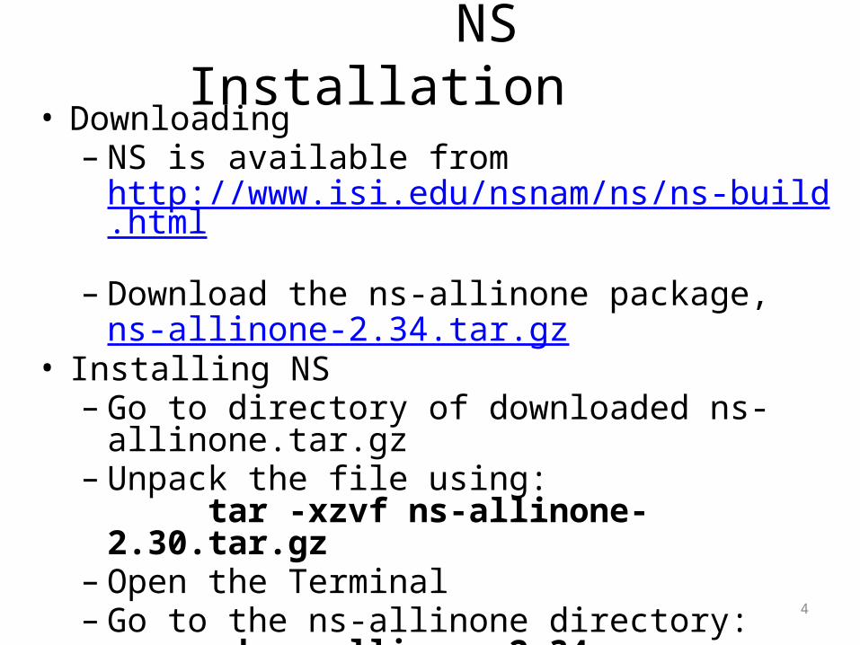
NS Installation

4

• Downloading– NS is available from

http://www.isi.edu/nsnam/ns/ns-build.html – Download the ns-allinone package,

ns-allinone-2.34.tar.gz • Installing NS

– Go to directory of downloaded ns-allinone.tar.gz – Unpack the file using:

tar -xzvf ns-allinone-2.30.tar.gz – Open the Terminal– Go to the ns-allinone directory:

cd ns-allinone-2.34– Install it with the command

./install

5

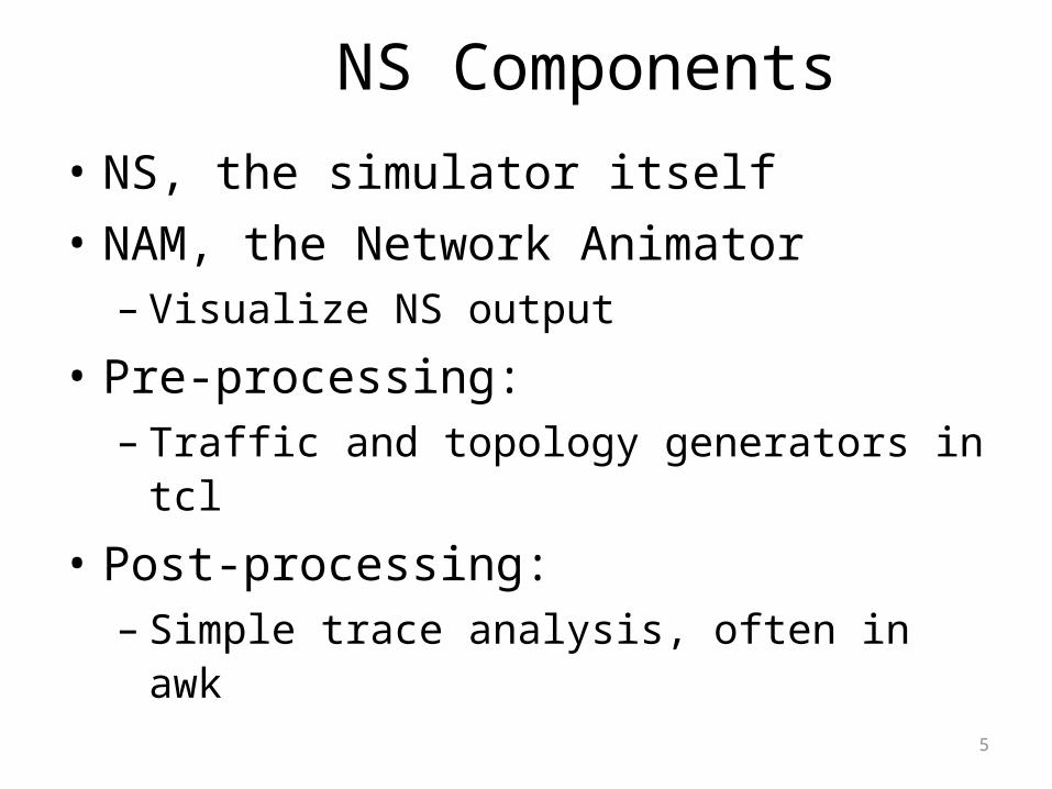
NS Components• NS, the simulator itself• NAM, the Network Animator

– Visualize NS output

• Pre-processing:– Traffic and topology generators in tcl

• Post-processing:– Simple trace analysis, often in awk

NAM : Network Animator

7

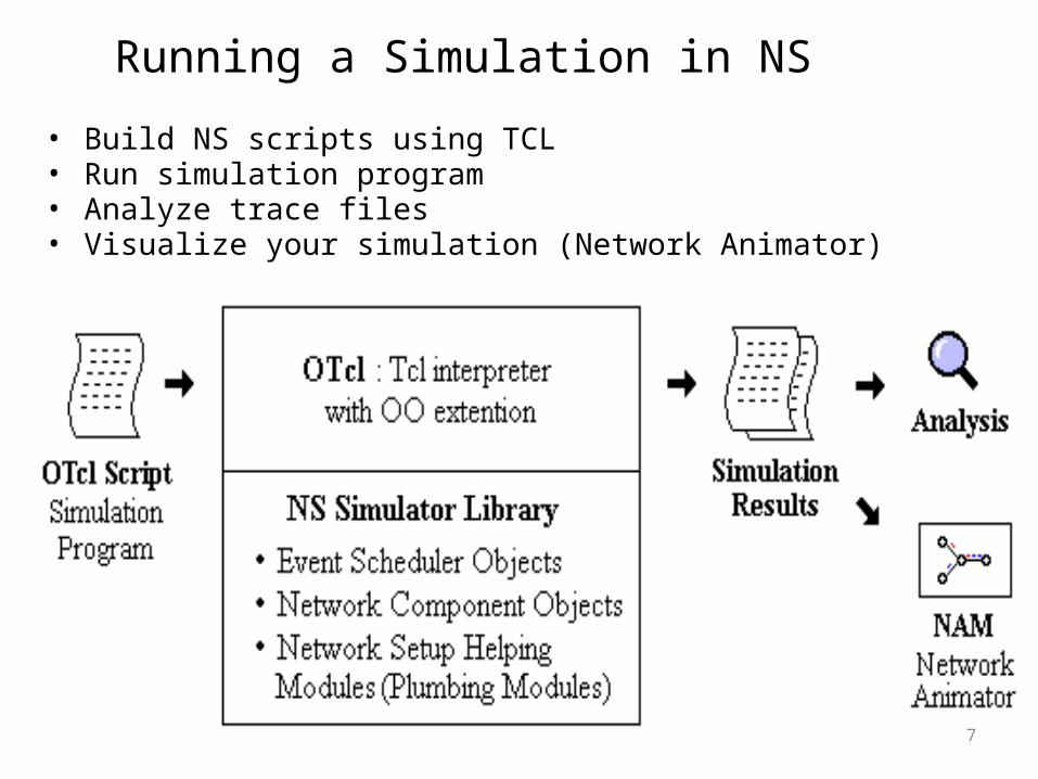
Running a Simulation in NS

• Build NS scripts using TCL• Run simulation program• Analyze trace files• Visualize your simulation (Network Animator)

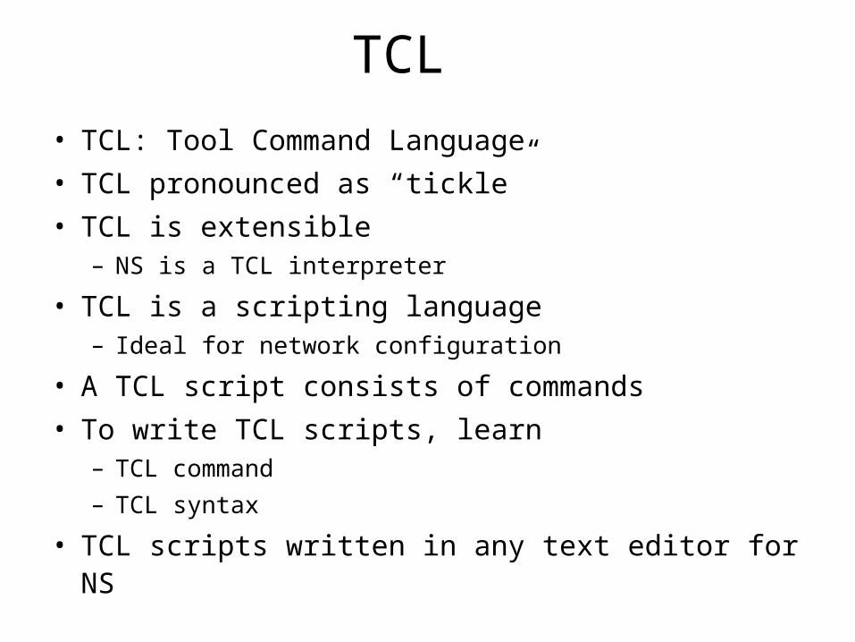
TCL• TCL: Tool Command Language• TCL pronounced as “tickle”• TCL is extensible

– NS is a TCL interpreter

• TCL is a scripting language– Ideal for network configuration

• A TCL script consists of commands• To write TCL scripts, learn

– TCL command– TCL syntax

• TCL scripts written in any text editor for NS

TCL Script for wireless Example

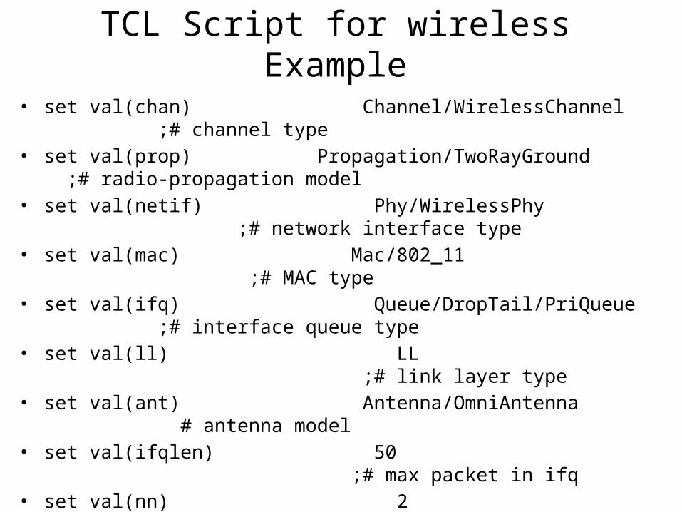
• set val(chan) Channel/WirelessChannel ;# channel type• set val(prop) Propagation/TwoRayGround ;# radio-propagation model• set val(netif) Phy/WirelessPhy ;# network interface type• set val(mac) Mac/802_11 ;# MAC type• set val(ifq) Queue/DropTail/PriQueue ;# interface queue type• set val(ll) LL ;# link layer type• set val(ant) Antenna/OmniAntenna # antenna model• set val(ifqlen) 50 ;# max packet in ifq• set val(nn) 2 ;# number of mobilenodes• set val(rp) DSDV ;# routing protocol• • This is the predetermined value for examples

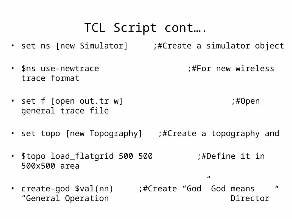
TCL Script cont….• set ns [new Simulator] ;#Create a simulator object

• $ns use-newtrace ;#For new wireless trace format

• set f [open out.tr w] ;#Open general trace file

• set topo [new Topography] ;#Create a topography and • $topo load_flatgrid 500 500 ;#Define it in 500x500 area

• create-god $val(nn) ;#Create “God” God means “General Operation Director”

TCL Script cont….

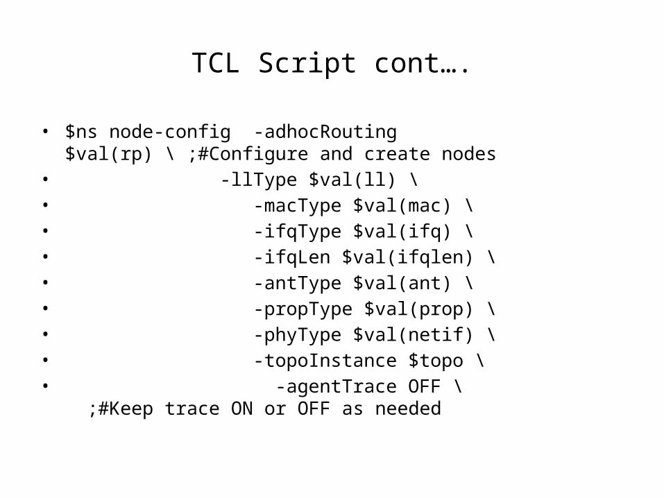
• $ns node-config -adhocRouting $val(rp) \ ;#Configure and create nodes• -llType $val(ll) \• -macType $val(mac) \• -ifqType $val(ifq) \• -ifqLen $val(ifqlen) \• -antType $val(ant) \• -propType $val(prop) \• -phyType $val(netif) \• -topoInstance $topo \• -agentTrace OFF \ ;#Keep trace ON or OFF as

needed

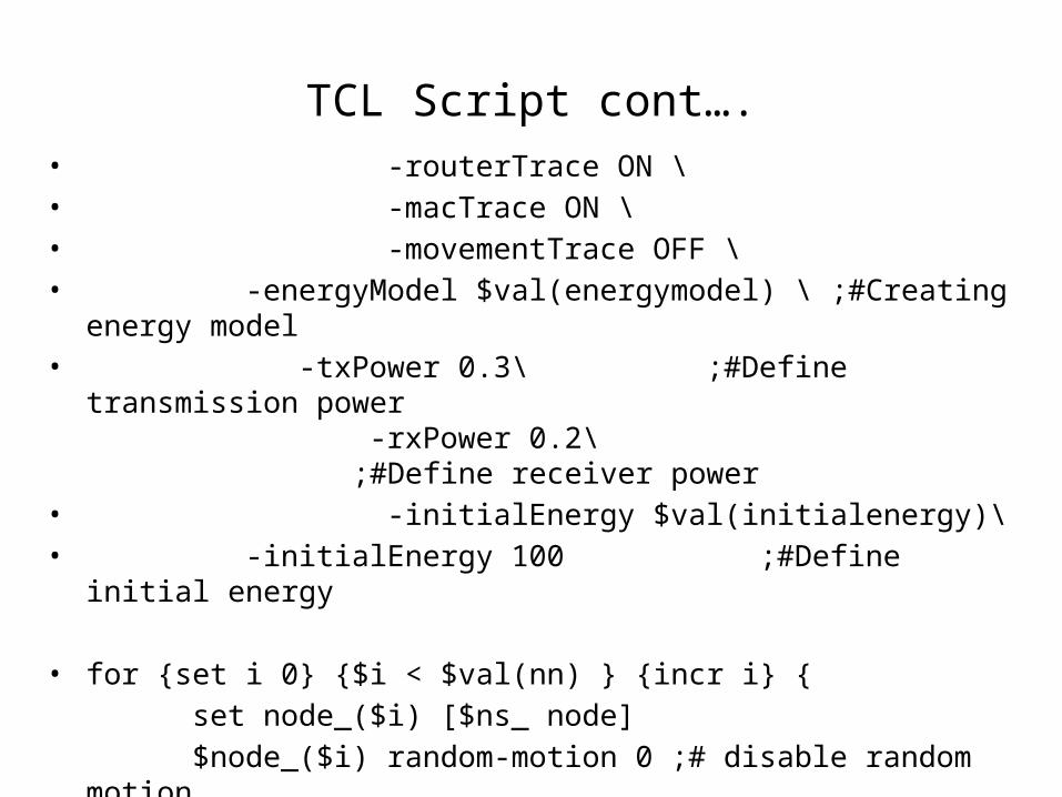
TCL Script cont….• -routerTrace ON \• -macTrace ON \• -movementTrace OFF \• -energyModel $val(energymodel) \ ;#Creating energy model• -txPower 0.3\ ;#Define transmission power

-rxPower 0.2\ ;#Define receiver power

• -initialEnergy $val(initialenergy)\• -initialEnergy 100 ;#Define initial energy

• for {set i 0} {$i < $val(nn) } {incr i} {set node_($i) [$ns_ node]$node_($i) random-motion 0 ;# disable random

motion}

TCL Script cont….

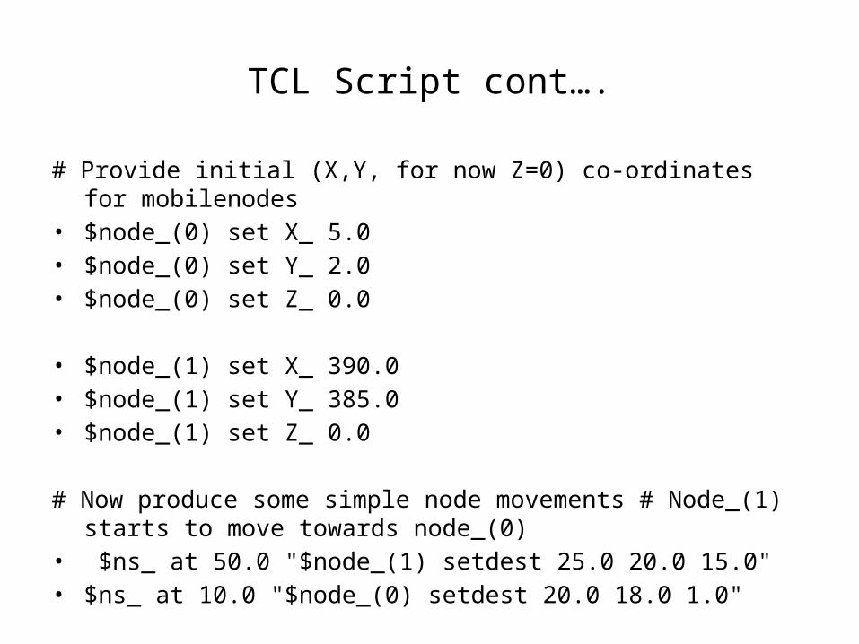
# Provide initial (X,Y, for now Z=0) co-ordinates for mobilenodes • $node_(0) set X_ 5.0• $node_(0) set Y_ 2.0• $node_(0) set Z_ 0.0 • $node_(1) set X_ 390.0• $node_(1) set Y_ 385.0• $node_(1) set Z_ 0.0 # Now produce some simple node movements # Node_(1) starts to move

towards node_(0)• $ns_ at 50.0 "$node_(1) setdest 25.0 20.0 15.0"• $ns_ at 10.0 "$node_(0) setdest 20.0 18.0 1.0"

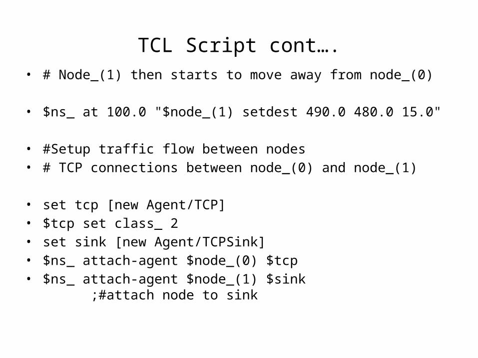
TCL Script cont….• # Node_(1) then starts to move away from node_(0)

• $ns_ at 100.0 "$node_(1) setdest 490.0 480.0 15.0"

• #Setup traffic flow between nodes• # TCP connections between node_(0) and node_(1) • set tcp [new Agent/TCP]• $tcp set class_ 2• set sink [new Agent/TCPSink]• $ns_ attach-agent $node_(0) $tcp• $ns_ attach-agent $node_(1) $sink ;#attach node to sink

TCL Script cont….

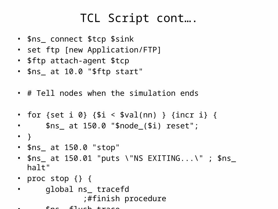
• $ns_ connect $tcp $sink• set ftp [new Application/FTP]• $ftp attach-agent $tcp• $ns_ at 10.0 "$ftp start"

• # Tell nodes when the simulation ends

• for {set i 0} {$i < $val(nn) } {incr i} {• $ns_ at 150.0 "$node_($i) reset";• }• $ns_ at 150.0 "stop"• $ns_ at 150.01 "puts \"NS EXITING...\" ; $ns_ halt"• proc stop {} {• global ns_ tracefd ;#finish procedure• $ns_ flush-trace

TCL Script cont….

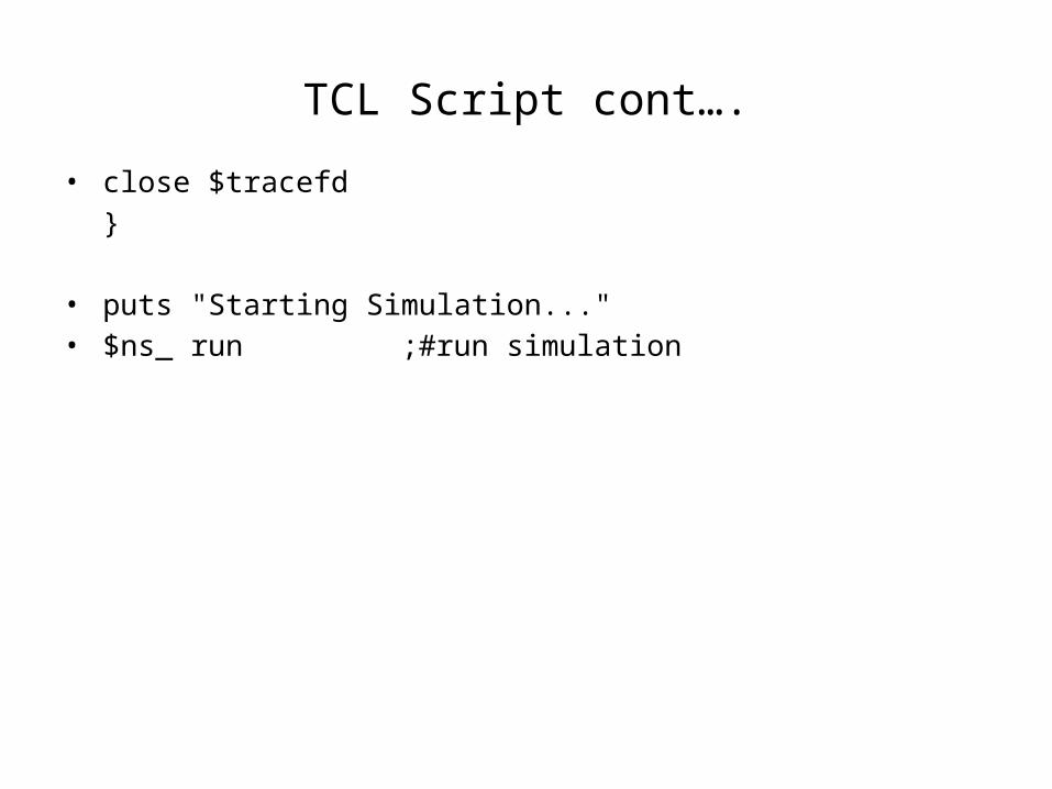
• close $tracefd}

• puts "Starting Simulation..."• $ns_ run ;#run simulation

Run simulation program

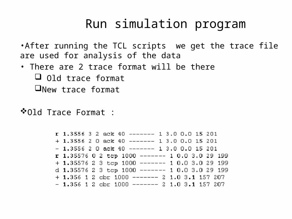
•After running the TCL scripts we get the trace file are used for analysis of the data • There are 2 trace format will be there

Old trace formatNew trace format

Old Trace Format :

Each trace line starts with an event (+, -, d, r) descriptor followed by the simulation time (in seconds) of that event, and from and to node, which identify the link on which the event occurred

The next information in the line before flags (appeared as "------" since no flag is set) is packet type and size (in Bytes).

After the flags there will be a flow id and source address, destination address , sequence number of the packet and the packet id will be there.

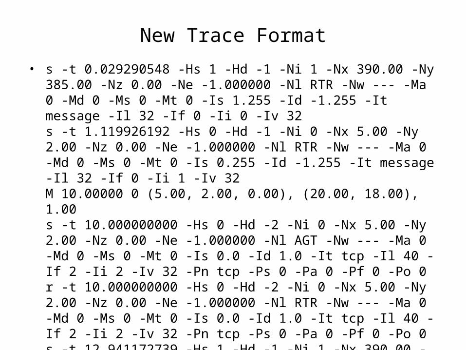
New Trace Format

• s -t 0.029290548 -Hs 1 -Hd -1 -Ni 1 -Nx 390.00 -Ny 385.00 -Nz 0.00 -Ne -1.000000 -Nl RTR -Nw --- -Ma 0 -Md 0 -Ms 0 -Mt 0 -Is 1.255 -Id -1.255 -It message -Il 32 -If 0 -Ii 0 -Iv 32 s -t 1.119926192 -Hs 0 -Hd -1 -Ni 0 -Nx 5.00 -Ny 2.00 -Nz 0.00 -Ne -1.000000 -Nl RTR -Nw --- -Ma 0 -Md 0 -Ms 0 -Mt 0 -Is 0.255 -Id -1.255 -It message -Il 32 -If 0 -Ii 1 -Iv 32 M 10.00000 0 (5.00, 2.00, 0.00), (20.00, 18.00), 1.00s -t 10.000000000 -Hs 0 -Hd -2 -Ni 0 -Nx 5.00 -Ny 2.00 -Nz 0.00 -Ne -1.000000 -Nl AGT -Nw --- -Ma 0 -Md 0 -Ms 0 -Mt 0 -Is 0.0 -Id 1.0 -It tcp -Il 40 -If 2 -Ii 2 -Iv 32 -Pn tcp -Ps 0 -Pa 0 -Pf 0 -Po 0 r -t 10.000000000 -Hs 0 -Hd -2 -Ni 0 -Nx 5.00 -Ny 2.00 -Nz 0.00 -Ne -1.000000 -Nl RTR -Nw --- -Ma 0 -Md 0 -Ms 0 -Mt 0 -Is 0.0 -Id 1.0 -It tcp -Il 40 -If 2 -Ii 2 -Iv 32 -Pn tcp -Ps 0 -Pa 0 -Pf 0 -Po 0 s -t 12.941172739 -Hs 1 -Hd -1 -Ni 1 -Nx 390.00 -Ny 385.00 -Nz 0.00 -Ne -1.000000 -Nl RTR -Nw --- -Ma 0 -Md 0 -Ms 0 -Mt 0 -Is 1.255 -Id -1.255 -It message -Il 32 -If 0 -Ii 3 -Iv 32 1.000000 -Nl RTR -Nw --- -Ma 0 -Md 0 -Ms 0 -Mt 0 -Is 0.0 -Id 1.0 -It tcp -Il 40 -If 2 -Ii 4 -Iv 32 -Pn tcp -Ps 0 -Pa 0 -Pf 0 -Po 0

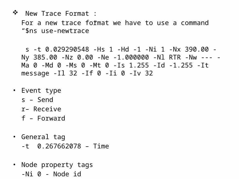
New Trace Format :For a new trace format we have to use a command “$ns use-newtrace”

s -t 0.029290548 -Hs 1 -Hd -1 -Ni 1 -Nx 390.00 -Ny 385.00 -Nz 0.00 -Ne -1.000000 -Nl RTR -Nw --- -Ma 0 -Md 0 -Ms 0 -Mt 0 -Is 1.255 -Id -1.255 -It message -Il 32 -If 0 -Ii 0 -Iv 32

• Event types – Sendr– Receivef – Forward

• General tag-t 0.267662078 – Time

• Node property tags-Ni 0 - Node id

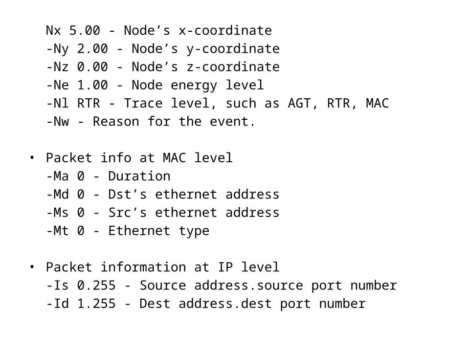
Nx 5.00 - Node’s x-coordinate-Ny 2.00 - Node’s y-coordinate-Nz 0.00 - Node’s z-coordinate-Ne 1.00 - Node energy level-Nl RTR - Trace level, such as AGT, RTR, MAC-Nw - Reason for the event.

• Packet info at MAC level -Ma 0 - Duration-Md 0 - Dst’s ethernet address-Ms 0 - Src’s ethernet address-Mt 0 - Ethernet type

• Packet information at IP level -Is 0.255 - Source address.source port number-Id 1.255 - Dest address.dest port number

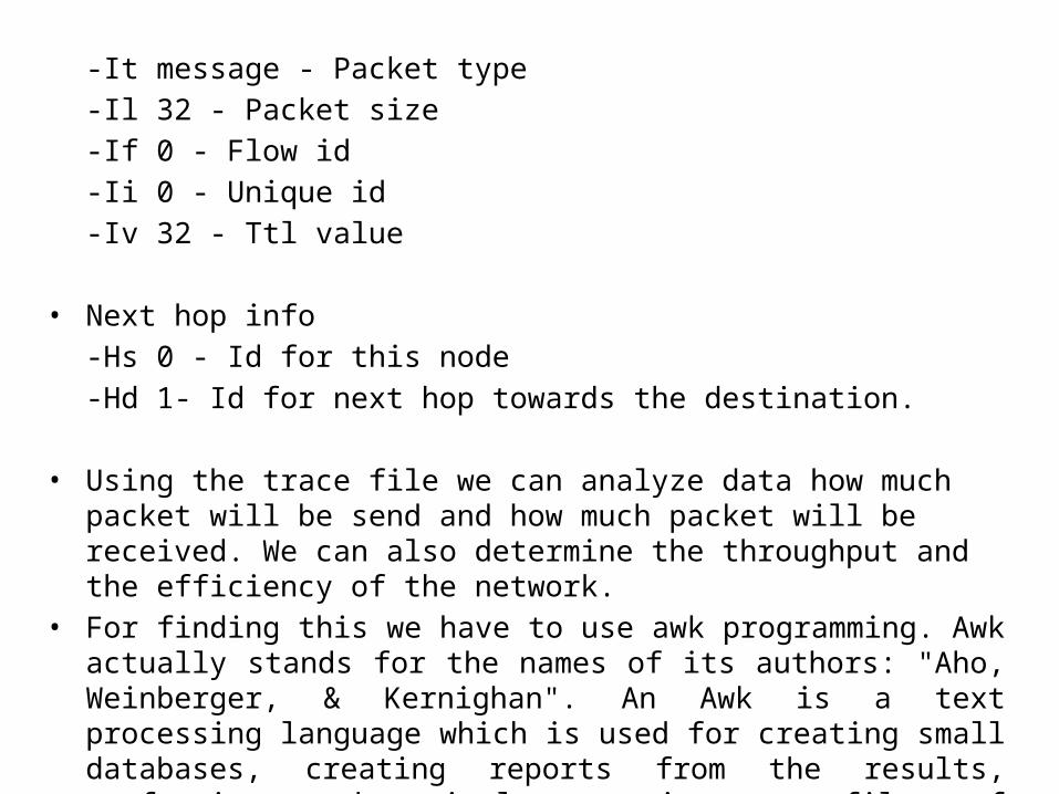
-It message - Packet type-Il 32 - Packet size-If 0 - Flow id-Ii 0 - Unique id-Iv 32 - Ttl value

• Next hop info-Hs 0 - Id for this node-Hd 1- Id for next hop towards the destination.

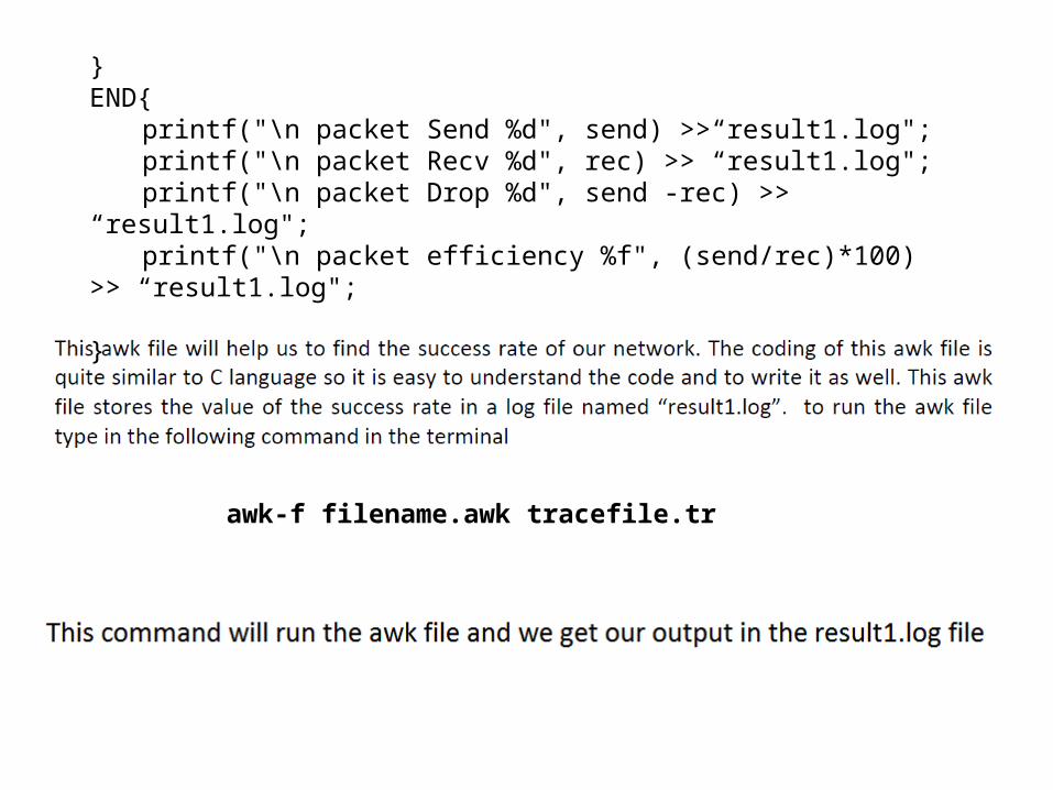
• Using the trace file we can analyze data how much packet will be send and how much packet will be received. We can also determine the throughput and the efficiency of the network.

• For finding this we have to use awk programming. Awk actually stands for the names of its authors: "Aho, Weinberger, & Kernighan". An Awk is a text processing language which is used for creating small databases, creating reports from the results, performing mathematical operations on files of numeric data .

AWKNow ,we will discussed the simple awk script for finding out the packet receive and sending.

BEGIN { rec = 0;send = 0;} {

if ( $1 == "s") {

send = send +1;

} if ( $1 == "r" ) {

rec = rec + 1;

}

awk-f filename.awk tracefile.tr

}END{

printf("\n packet Send %d", send) >>“result1.log";printf("\n packet Recv %d", rec) >> “result1.log";printf("\n packet Drop %d", send -rec) >> “result1.log";printf("\n packet efficiency %f", (send/rec)*100) >> “result1.log";

}

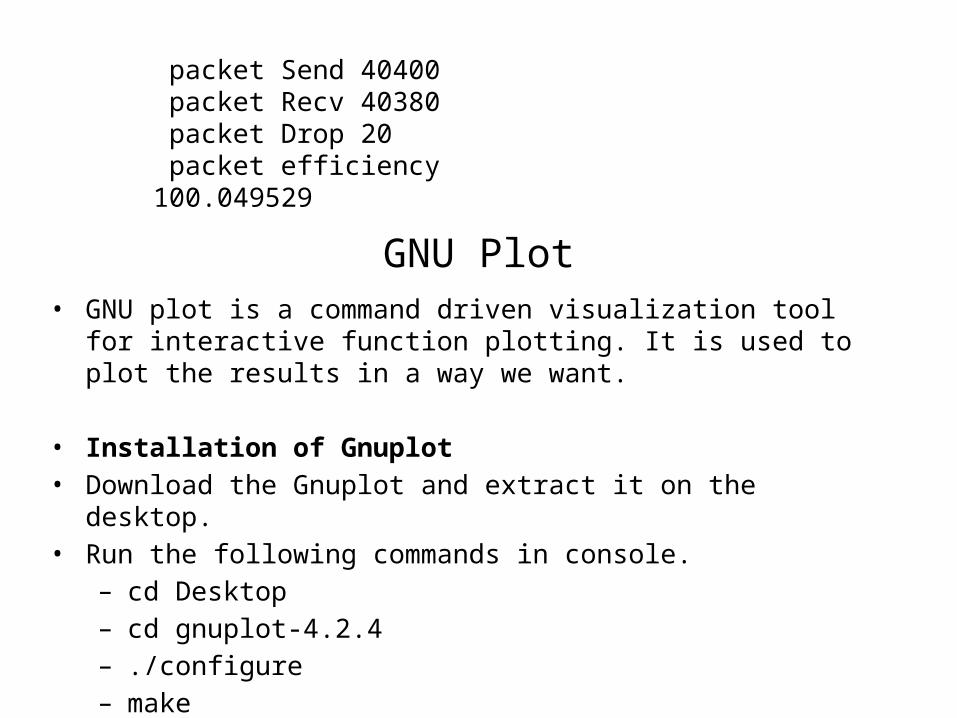
packet Send 40400 packet Recv 40380 packet Drop 20 packet efficiency 100.049529

GNU Plot• GNU plot is a command driven visualization tool for interactive function

plotting. It is used to plot the results in a way we want.

• Installation of Gnuplot• Download the Gnuplot and extract it on the desktop.• Run the following commands in console.

– cd Desktop– cd gnuplot-4.2.4– ./configure– make– make install

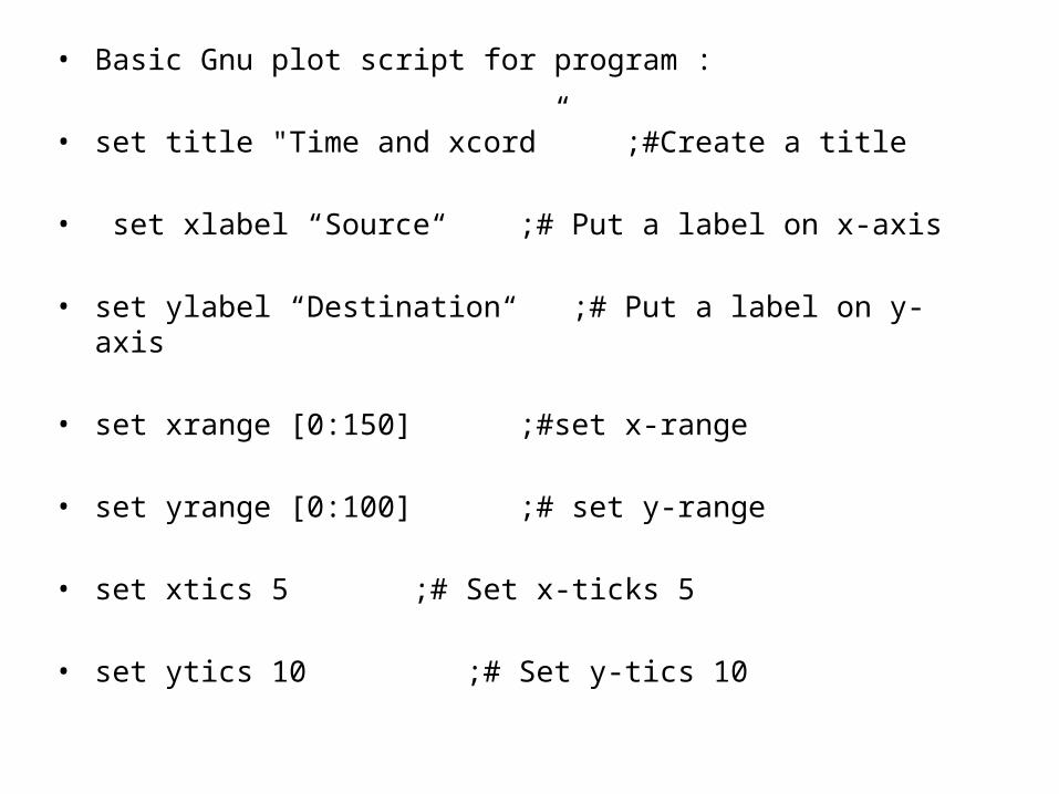
• Basic Gnu plot script for program :

• set title "Time and xcord” ;#Create a title

• set xlabel “Source“ ;# Put a label on x-axis

• set ylabel “Destination“ ;# Put a label on y-axis

• set xrange [0:150] ;#set x-range

• set yrange [0:100] ;# set y-range

• set xtics 5 ;# Set x-ticks 5

• set ytics 10 ;# Set y-tics 10

• plot "thr3.log" using 1:2 title "node" with linespoints ;#Data to be plotted

• pause -1 "Hit return to continue“ ;# pause a graph upto hit from

keyboard

• For plotting the graph time v/s x-cordinates first we have to take a data of it in a separate file. For this we also write awk program which dissuced below:

• Begin {

time = $3; ;# data extracted from 3rd columnxcord = $11; ;#data extracted from 11th column

}end{

printf("\n %f", time) >>"thr3.log"; ;# print data in thr.log fileprintf(" %f", xcord) >>"thr3.log";

}

•

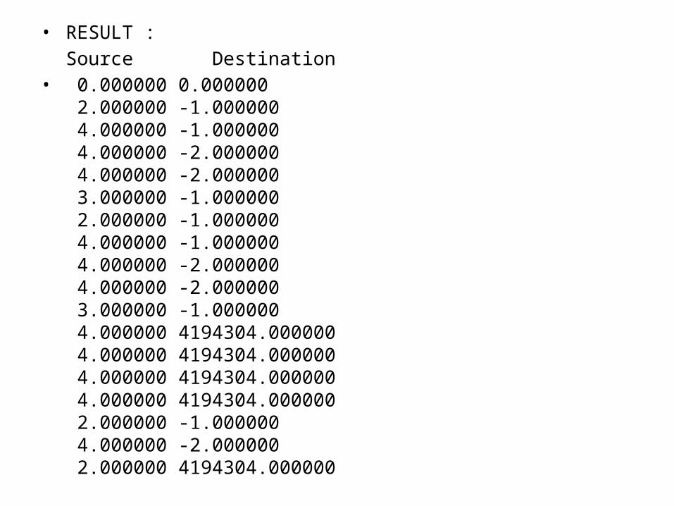
• RESULT :Source Destination

• 0.000000 0.000000 2.000000 -1.000000 4.000000 -1.000000 4.000000 -2.000000 4.000000 -2.000000 3.000000 -1.000000 2.000000 -1.000000 4.000000 -1.000000 4.000000 -2.000000 4.000000 -2.000000 3.000000 -1.000000 4.000000 4194304.000000 4.000000 4194304.000000 4.000000 4194304.000000 4.000000 4194304.000000 2.000000 -1.000000 4.000000 -2.000000 2.000000 4194304.000000

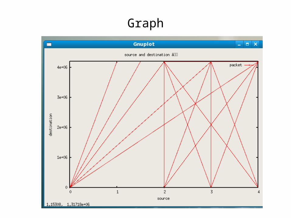
Graph

Conclusion

After working on this project we face a many difficulties because this linux environment is not familiar with us. We also not familiar with network simulator and Awk programming tool. But the guidance of the Prof. Sachin Gajjar and our senior Maunik Sorthiya make it as simple as possible. We heartly thankful to them.

THANK YOU