network structure explains the impact of attitudes on ...(freeman, 1978; opsahl, agneessens, &...

Network Structure Explains the Impact of Attitudes on VotingDecisionsJonas Dalege, Denny Borsboom, Frenk van Harreveld, Lourens J. Waldorp & Han L. J. van der Maas

Department of Psychology, University of Amsterdam, 1018 WT Amsterdam, The Netherlands

Attitudes can have a profound impact on socially relevant behaviours, such as voting. However, this effect is not uni-form across situations or individuals, and it is at present difficult to predict whether attitudes will predict behaviourin any given circumstance. Using a network model, we demonstrate that (a) more strongly connected attitude networkshave a stronger impact on behaviour, and (b) within any given attitude network, the most central attitude elementshave the strongest impact. We test these hypotheses using data on voting and attitudes toward presidential candi-dates in the US presidential elections from 1980 to 2012. These analyses confirm that the predictive value of attitudenetworks depends almost entirely on their level of connectivity, with more central attitude elements having strongerimpact. The impact of attitudes on voting behaviour can thus be reliably determined before elections take place byusing network analyses.

S uppose you are one of the more than 130 million Amer-icans who voted in the presidential election in 2016.Let us further assume that you were supportive of

Hillary Clinton: You mostly held positive beliefs (e.g., youthought she was a good leader and a knowledgeable person)and you had positive feelings toward her (e.g., she madeyou feel hopeful and proud), representing a positive atti-tude toward Hillary Clinton (Dalege et al., 2016; Eagly &Chaiken, 1993; Fishbein & Ajzen, 1975; Rosenberg, Hov-land, McGuire, & Brehm, 1960). However, you also helda few negative beliefs toward her (e.g., you thought thatHillary Clinton was not very honest). Did your overall pos-itive attitude cause you to vote for Hillary Clinton? Herewe show that the answer to this question depends on thenetwork structure of your attitude: First, we show that theimpact of attitudes (i.e., average of the attitude elements)on behavioural decisions depends on the connectivity of theattitude network (e.g., your the network of your positiveattitude toward Hillary Clinton was highly connected, soyou probably voted for Hillary Clinton). Second, we showthat central attitude elements have a stronger impact on be-havioural decisions than peripheral attitude elements (e.g.,your positive beliefs about Hillary Clinton were more centralin your attitude network than your negative beliefs, so thechance that you voted for Hillary Clinton further increased).We thus provide insight into how structural properties of at-titudes determine the extent to which attitudes have impacton behaviour.

In network theory, dynamical systems are modelled as aset of nodes, representing autonomous entities, and edges,representing interactions between the nodes (Newman,2010). The set of nodes and edges jointly defines a networkstructure. Modelling complex systems in this way has prob-ably become the most promising data-analytic tool to tacklecomplexity in many fields (Barabasi, 2011), such as physics(Barabasi & Albert, 1999; Watts & Strogatz, 1998), biology

(Barabasi & Zoltan, 2004), and psychology (Cramer, Wal-dorp, van der Maas, & Borsboom, 2010; Cramer et al., 2012;van de Leemput et al., 2014; van Borkulo et al., 2015). Re-cently, network analysis has also been introduced to the re-search on attitudes in the form of the Causal Attitude Net-work (CAN) model (Dalege et al., 2016). In this model, at-titudes are conceptualized as networks, in which nodes rep-resent attitude elements that are connected by direct causalinteractions (see Figure 1). The CAN model further assumesthat the Ising model (Ising, 1925), which originated from sta-tistical physics, represents an idealized model of attitude dy-namics.

In the Ising model, the probability of configurations (i.e.,the states of all nodes in the network), which represents theoverall state of the attitude network, depends on the amountof energy of a given configuration. The energy of a given con-figuration can be calculated using the Hamiltonian function:

H(x) = −∑i

τixi −∑<i,j>

ωixixj . (1)

Here, k distinct attitude elements 1,....,i,j,....k are representedas nodes that engage in pairwise interactions; the variablesxi and xj represent the states of nodes i and j respectively.The model is designed to represent the probability of thesestates as a function of a number of parameters that encodethe network structure. The parameter τi is the threshold ofnode i, which determines the disposition of that node to bein a positive state (1; endorsing an attitude element) or neg-ative state (-1, not endorsing an attitude element) regardlessof the state of the other nodes in the network (statistically,this parameter functions as an intercept). The parameter ωirepresents the edge weight (i.e., the strength of interaction)between nodes i and j. As can be seen in this equation, theHamiltonian energy decreases if nodes are in a state that iscongruent with their threshold and when two nodes havingpositive (negative) edge weights assume the same (different)

1

arX

iv:1

704.

0091

0v2

[cs

.SI]

6 S

ep 2

017

B1 B2

F1

F2

B3

B4

B5

F3

B6

F4

D

B1 B2

F1

F2

B3

B4

B5

F3

B6

F4

D

B1 B2

F1

F2

B3

B4

B5

F3

B6

F4

D

Temperature

Estimated Correlation Networks

True Underlying Causal Network

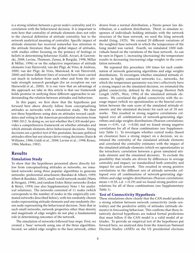
Figure 1: Illustrations of the Causal Attitude Network model and the hypotheses of the current study. Networks rep-resent a hypothetical attitude network toward a presidential candidate consisting of six beliefs (e.g., judging the candidateas honest, intelligent, caring; represented by nodes B1 to B6), four feelings (e.g., feeling hope, anger toward the candidate;represented by nodes F1 to F4), and the voting decision (represented by the node D). Red nodes within the dashed squarerepresent the part of the network on which connectivity and centrality estimates are calculated. Edges represent positivebidirectional causal influences (correlations) in the causal network (correlation networks), with thicker edges representinghigher influence (correlations). Note that in this network, we assume that positive (negative) states of all nodes indicatea positive (negative) evaluation (e.g., positive state of judging a candidate as honest (dishonest) would be to (not) endorsethis judgment). Size of the red nodes corresponds to their closeness centrality (see Methods for details on the network de-scriptives). In the CAN model, temperature represents a formalized conceptualization of consistency pressure on attitudenetworks. The correlation networks illustrate that lower (higher) temperature implies higher (lower) correlations betweenthe attitude elements. 2

state. Assuming that attitude elements of the same (differ-ent) valence are generally positively (negatively) connected,attitude networks thus strive for a consistent representationof the attitude. The probability of a given configuration canbe calculated using the Gibbs distribution (Murphy, 2012):

Pr(X = x) =exp(−βH(x)

Z, (2)

in which β represents the inverse temperature of the sys-tem, which can be seen as consistency pressures on attitudenetworks: reducing (increasing) the temperature of the sys-tem results in stronger (weaker) influence of the thresholdsand weights, thereby scaling the entropy of the Ising net-work model (Epskamp, Maris, Waldorp, & Borsboom, 2016;Wainwright & Jordan, 2008). An Ising model with low (high)temperature results in a highly (weakly) connected correla-tion network (see Figure 1). The denominator Z representsthe sum of the energies of all possible configurations, whichacts as a normalising factor to ensure that the sum of theprobabilities adds up to 1.

Conceptualising attitudes as Ising models allows for thederivation of several hypotheses and a crucial test of thisconceptualisation is whether it can advance the understand-ing of the relation between attitudes and behavioural deci-sions. In the present paper we apply the CAN model and arethe first to (a) formalize and (b) test hypotheses based on theCAN model regarding the impact of attitudes on behaviour.

The impact of attitudes on behaviour has been one ofthe central research themes in Social Psychology in re-cent decades (Ajzen, 1991; Glasman & Albarracın, 2006;Kruglanski et al., 2015). The bulk of the research on therelation between attitudes and behaviour has been done un-der the umbrella definition of attitude strength, which holdsthat one central feature of strong attitudes is that they havea strong impact on behaviour (Krosnick & Petty, 1995). Sev-eral lines of research have identified factors related to atti-tude strength. Among the most widely researched of theseare attitude accessibility, attitude importance, and attitudi-nal ambivalence. Studies have shown that accessible atti-tudes (i.e., attitudes that can be easily retrieved from mem-ory) have more impact on behaviour (Fazio & Williams,1986; Glasman & Albarracın, 2006). Similarly, higher levelsof (subjective) attitude importance (i.e., attitudes, to whicha person attaches subjective importance), are related to in-creased accessibility of attitudes (Krosnick, 1989) and tohigher levels of consistency between attitudes and behaviour(Krosnick, 1988; Visser, Krosnick, & Simmons, 2003). Am-bivalent attitudes (i.e., attitudes that are based on both neg-ative and positive associations) are less predictive of be-haviour than univalent attitudes (Armitage & Conner, 2000;van Harreveld, Nohlen, & Schneider, 2015). While theseand other attitude strength attributes, such as certainty andextremity, are generally interrelated (Krosnick, Boninger,Chuang, Berent, & Carnot, 1993; Visser, Bizer, & Krosnick,

2006), a framework that unifies these different attributes haslong been absent in the literature. Recently, however, basedon the development of the CAN model, attitude strength wasformally conceptualized as network connectivity (Dalege etal., 2016). The CAN model might thus provide the basis fora comprehensive and formalized framework of the relation-ship between attitudes and behaviour. Our current aim isto develop and test such a framework. To do so, we first for-mally derive hypotheses regarding the impact of attitudes onbehaviour from the CAN model. Second, we test these hy-potheses in the context of voting decisions in the US Ameri-can presidential elections.

From the CAN model the hypothesis follows that highlyconnected attitude networks (i.e., attitude networks that arebased on Ising models with low temperature) have a strongimpact on behaviour. As can be seen in Figure 1, low tem-perature results in strong connections both between non-behavioural attitude elements (i.e., beliefs and feelings) andbetween non-behavioural attitude elements and behaviours(e.g., behavioural decisions) (Dalege et al., 2016). Attitudeelements in highly connected networks are thus expected tohave a strong impact on behavioural decisions. This leadsto the hypothesis that the overall impact of attitudes de-pends on the connectivity of the attitude network. Whilethe connectivity of attitude networks provides a novel for-malisation of attitude strength, earlier approaches to under-standing the structure of attitudes fit very well within thisframework. For example, studies have shown that impor-tant attitudes are more coherent than unimportant attitudes(Judd, Krosnick, & Milburn, 1981; Judd & Krosnick, 1989)and that strong attitudes have a more consistent structurebetween feelings and beliefs than weak attitudes (Chaiken,Pomerantz, & Giner-Sorolla, 1995). Also, Phillip E. Con-verse’s (1970) distinction between attitudes and nonattitudesbased on stability of responses relates to our connectivityframework (Dalege et al., 2016)

In addition to predicting the overall impact of an atti-tude from the connectivity of the attitude network, the CANmodel predicts that the specific impact of attitude elementsdepends on their centrality (as defined by their closeness).Closeness refers to how strongly a given node is connectedboth directly and indirectly to all other nodes in the network(Freeman, 1978; Opsahl, Agneessens, & Skvoretz, 2010). Incontrast to connectivity, which represents a measure of thewhole network, centrality is a measure that applies to indi-vidual nodes within the network. Attitude elements high incloseness are good proxies of the overall state of the attitudenetwork, as they hold more information about the rest of thenetwork than peripheral attitude elements, rendering close-ness the optimal measure of centrality for our current pur-poses. We therefore expect central attitude elements to havea stronger impact (directly or indirectly) on a behaviouraldecision no matter which attitude elements are direct causesof this decision. This can also be seen in Figure 1, as there

3

is a strong relation between a given node’s centrality and it’scorrelation with the behavioural decision. It is important tonote here that centrality of attitude elements does not referto the classical definition of attitude centrality, but to thenetwork analytical meaning of centrality. Specific impact ofattitude elements has received somewhat less attention inthe attitude literature than the global impact of attitudes,with studies either focusing on the primacy of feelings orbeliefs in determining behaviour (Galdi, Arcuri, & Gawron-ski, 2008; Lavine, Thomsen, Zanna, & Borgida, 1998; Millar& Millar, 1996) or on the subjective importance of attitudeelements (van Harreveld, van der Pligt, de Vries, & Andreas,2000; van der Pligt, de Vries, Manstead, & van Harreveld,2000) and these different lines of research have been carriedout much in isolation from each other and from the atti-tude strength research paradigm (for an exception see vanHarreveld et al., 2000). It is our view that an advantage ofthe approach we take in this article is that our frameworkholds promise in unifying these different approaches to un-derstanding the relation between attitudes and behaviour.

In this paper, we first show that the hypotheses putforward here above directly follow from conceptualisingattitudes as networks with a simulation study. We thentest these hypotheses using data on attitudes toward candi-dates and voting in the American presidential elections from1980-2012. In doing so, we test whether the CAN model pro-vides a comprehensive framework on whether attitudes andwhich attitude elements drive behavioural decisions. Votingdecisions are a perfect test of this postulate, because politicalattitudes often but not always drive voting decisions (Fazio &Williams, 1986; Galdi et al., 2008; Lavine et al., 1998; Kraus,1986; Markus, 1982).

ResultsSimulation StudyTo show that the hypotheses presented above directly fol-low from conceptualising attitudes as networks, we simu-lated networks using three popular algorithms to generatenetworks: preferential attachment (Barabasi & Albert, 1999;Albert & Barabasi, 2002), small-world network model (Watts& Strogatz, 1998), and random Erdos-Renyi networks (Erdos& Renyi, 1959) (see also Supplementary Note 1 for analyt-ical solutions). The networks consisted of 11 nodes (whichcorresponds to the number of nodes in the empirically esti-mated networks described below), with ten randomly chosennodes representing attitude elements and one randomly cho-sen node representing the behavioural decision. Note that insuch small networks, network properties other than densityand magnitude of edge weights do not play a fundamentalrole in determining outcomes of the network.

The simulation of networks followed four steps: First, wecreated a ’base’ network using one of the three algorithms.Second, we added edge weights to the base network, either

drawn from a normal distribution, a Pareto power law dis-tribution, or a uniform distribution. Third, to simulate re-sponses of individuals holding attitudes with the networkstructure of the base network, we used the Ising networkmodel (Ising, 1925). We created 20 different variations ofthe weighted base network in which the temperature of theIsing model was varied. Fourth, we simulated 1000 indi-viduals based on the variations of the base network. As canbe seen in Figure 1, increasing (decreasing) the temperatureresults in decreasing (increasing) edge weights in the corre-lation networks.

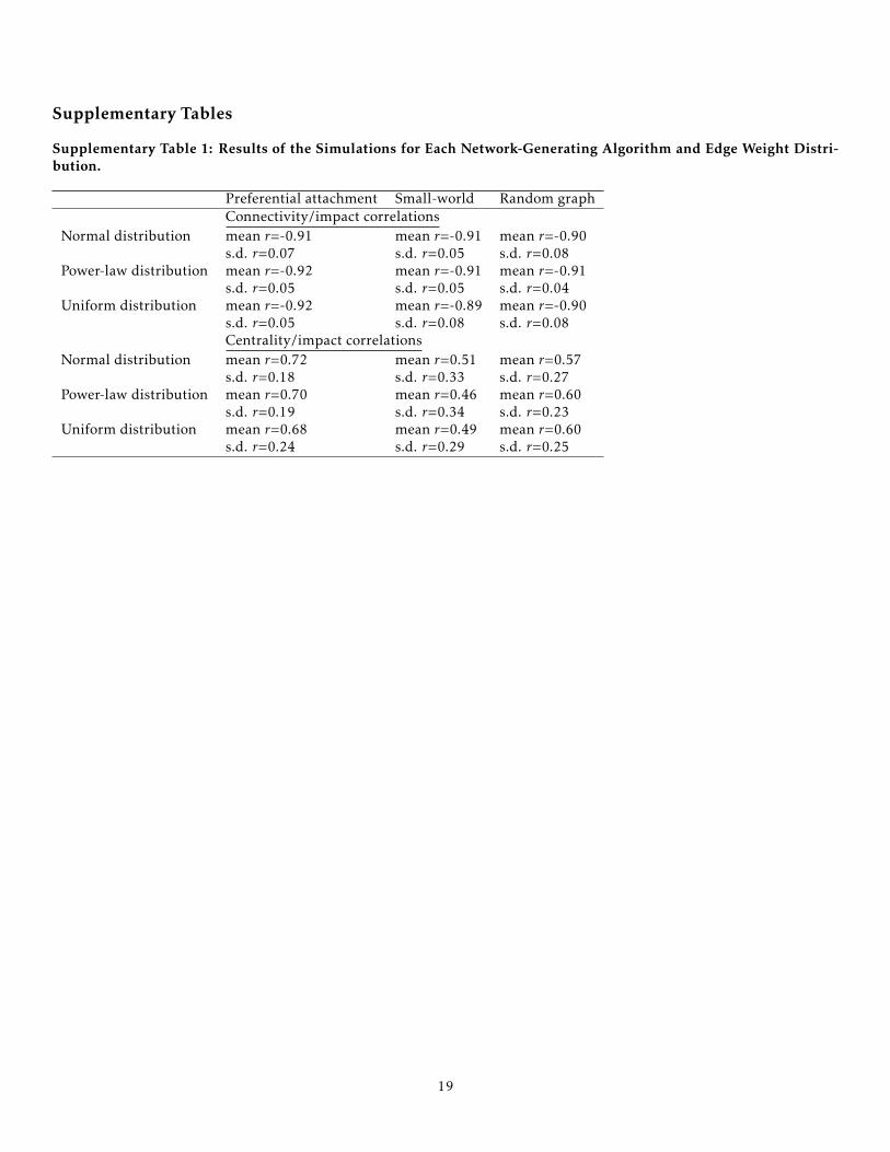
We repeated this procedure 100 times for each combi-nation of network generating algorithms and edge weightsdistributions. To investigate whether simulated attitude el-ements in highly connected networks (i.e., networks, forwhich the temperature parameter was low) collectively havea strong impact on the simulated decision, we estimated theglobal connectivity, defined by the Average Shortest PathLength (ASPL, West, 1996) of the simulated attitude ele-ments. We correlated the global connectivity with the av-erage impact (which we operationalize as the biserial corre-lation between the sum score of the simulated attitude el-ements and the simulated decision) for each set of 20 net-works. This resulted in strong negative correlations col-lapsed over all combinations of network-generating algo-rithms and edge weights distributions (Pearson correlations:mean r=-0.91, s.d. r=0.06) and we found strong negativecorrelations for all of these combinations (see Supplemen-tary Table 1). To investigate whether central nodes (basedon closeness) have a strong impact on a decision, we es-timated the centrality of the simulated attitude elementsand correlated the centrality estimates with the impact ofthe simulated attitude elements (which we operationalize asthe tetrachoric correlation between a given simulated atti-tude element and the simulated decision). To exclude thepossibility that results are driven by differences in averagecentrality and impact, we standardized both centrality andimpact for each network. This resulted in strong positivecorrelations in the different sets of attitude networks col-lapsed over all combinations of network-generating algo-rithms and edge weights distributions (Pearson correlations:mean r=0.59, s.d. r=0.29) and we found strong positive cor-relations for all of these combinations (see SupplementaryTable 1).

Test of Connectivity HypothesisThese simulations show clearly that the CAN model predictsa strong relation between network connectivity (node cen-trality) and the predictive utility of attitudes (attitude ele-ments) in forecasting behaviour. This confirms that these in-tuitively derived hypotheses are indeed formal predictionsthat must follow if the CAN model is a valid model of at-titudes. To provide an empirical test of the hypotheses putforward here, we analysed data from the American NationalElection Studies (ANES) on the US presidential elections

4

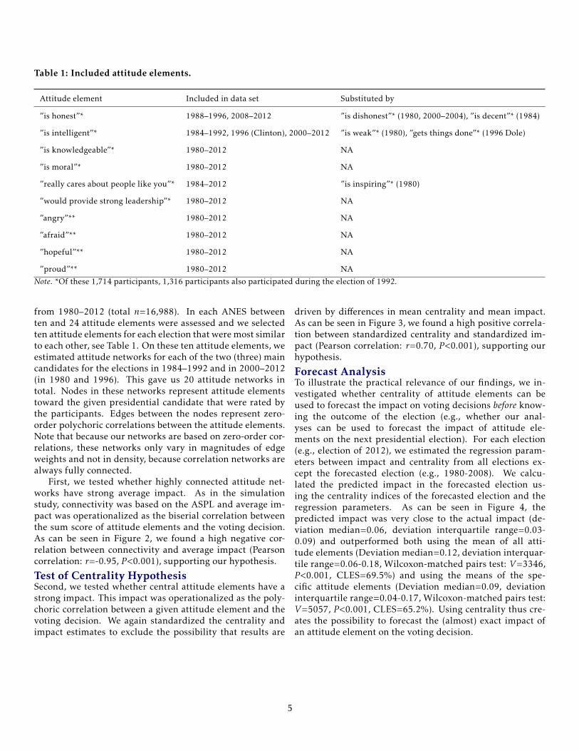
Table 1: Included attitude elements.

Attitude element Included in data set Substituted by

”is honest”* 1988–1996, 2008–2012 ”is dishonest”* (1980, 2000–2004), ”is decent”* (1984)

”is intelligent”* 1984–1992, 1996 (Clinton), 2000–2012 ”is weak”* (1980), ”gets things done”* (1996 Dole)

”is knowledgeable”* 1980–2012 NA

”is moral”* 1980–2012 NA

”really cares about people like you”* 1984–2012 ”is inspiring”* (1980)

”would provide strong leadership”* 1980–2012 NA

”angry”** 1980–2012 NA

”afraid”** 1980–2012 NA

”hopeful”** 1980–2012 NA

”proud”** 1980–2012 NA

Note. *Of these 1,714 participants, 1,316 participants also participated during the election of 1992.

from 1980–2012 (total n=16,988). In each ANES betweenten and 24 attitude elements were assessed and we selectedten attitude elements for each election that were most similarto each other, see Table 1. On these ten attitude elements, weestimated attitude networks for each of the two (three) maincandidates for the elections in 1984–1992 and in 2000–2012(in 1980 and 1996). This gave us 20 attitude networks intotal. Nodes in these networks represent attitude elementstoward the given presidential candidate that were rated bythe participants. Edges between the nodes represent zero-order polychoric correlations between the attitude elements.Note that because our networks are based on zero-order cor-relations, these networks only vary in magnitudes of edgeweights and not in density, because correlation networks arealways fully connected.

First, we tested whether highly connected attitude net-works have strong average impact. As in the simulationstudy, connectivity was based on the ASPL and average im-pact was operationalized as the biserial correlation betweenthe sum score of attitude elements and the voting decision.As can be seen in Figure 2, we found a high negative cor-relation between connectivity and average impact (Pearsoncorrelation: r=-0.95, P<0.001), supporting our hypothesis.

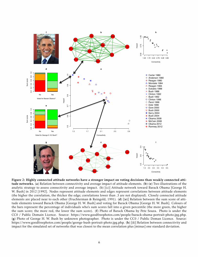
Test of Centrality HypothesisSecond, we tested whether central attitude elements have astrong impact. This impact was operationalized as the poly-choric correlation between a given attitude element and thevoting decision. We again standardized the centrality andimpact estimates to exclude the possibility that results are

driven by differences in mean centrality and mean impact.As can be seen in Figure 3, we found a high positive correla-tion between standardized centrality and standardized im-pact (Pearson correlation: r=0.70, P<0.001), supporting ourhypothesis.

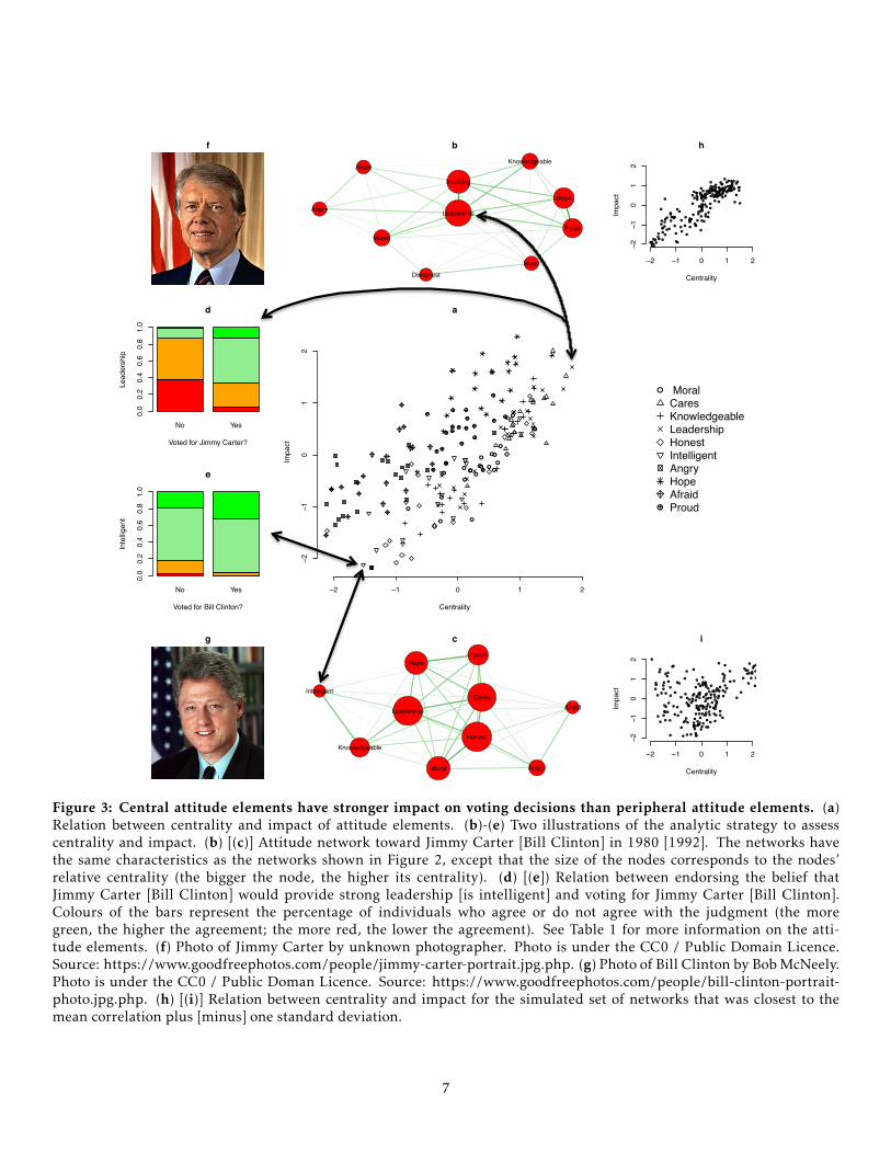
Forecast AnalysisTo illustrate the practical relevance of our findings, we in-vestigated whether centrality of attitude elements can beused to forecast the impact on voting decisions before know-ing the outcome of the election (e.g., whether our anal-yses can be used to forecast the impact of attitude ele-ments on the next presidential election). For each election(e.g., election of 2012), we estimated the regression param-eters between impact and centrality from all elections ex-cept the forecasted election (e.g., 1980-2008). We calcu-lated the predicted impact in the forecasted election us-ing the centrality indices of the forecasted election and theregression parameters. As can be seen in Figure 4, thepredicted impact was very close to the actual impact (de-viation median=0.06, deviation interquartile range=0.03-0.09) and outperformed both using the mean of all atti-tude elements (Deviation median=0.12, deviation interquar-tile range=0.06-0.18, Wilcoxon-matched pairs test: V=3346,P<0.001, CLES=69.5%) and using the means of the spe-cific attitude elements (Deviation median=0.09, deviationinterquartile range=0.04-0.17, Wilcoxon-matched pairs test:V=5057, P<0.001, CLES=65.2%). Using centrality thus cre-ates the possibility to forecast the (almost) exact impact ofan attitude element on the voting decision.

5

f

Moral

Cares

Knowledgeable

LeadershipHonest

IntelligentAngry

Hope Afraid

Proud

b

No Yes

Voted for Barack Obama?

Sum

sco

re

0.0

0.2

0.4

0.6

0.8

1.0

d

●

●

●

1.3 1.7 2.1 2.5 2.9

0.5

0.6

0.7

0.8

0.9

1.0

Connectivity

Impa

ct

a

No Yes

Voted for George H. W. Bush?

Sum

sco

re

0.0

0.2

0.4

0.6

0.8

1.0

e

g

Intelligent

Moral

Leadership

CaresKnowledgeable

Honest

Angry

Hope

AfraidProud

c

●

●

●

Carter 1980Anderson 1980Reagan 1980Mondale 1984Reagan 1984Dukakis 1988Bush 1988Clinton 1992Bush 1992Clinton 1996Perot 1996Dole 1996Gore 2000Bush 2000Kerry 2004Bush 2004Obama 2008McCain 2008Obama 2012Romney 2012

●●

●

●

●

●

●

●

●

●●

●

●

●

●

●

●

●

●

●

1.20 1.72 2.24 2.76 3.28 3.80

0.50

0.75

1.00

Connectivity

Impa

ct

h

●

● ●

●

●

●

●●

●

●

●

●

●

●●

●

●

●

●

●

1.5 2.5 3.5 4.5 5.5 6.5

0.3

0.6

0.9

Connectivity

Impa

ct

i

Figure 2: Highly connected attitude networks have a stronger impact on voting decisions than weakly connected atti-tude networks. (a) Relation between connectivity and average impact of attitude elements. (b)-(e) Two illustrations of theanalytic strategy to assess connectivity and average impact. (b) [(c)] Attitude network toward Barack Obama [George H.W. Bush] in 2012 [1992]. Nodes represent attitude elements and edges represent correlations between attitude elements(the higher the correlation, the thicker the edge; correlations lower than .3 are not displayed). Closely connected attitudeelements are placed near to each other (Fruchterman & Reingold, 1991). (d) [(e)] Relation between the sum score of atti-tude elements toward Barack Obama [George H. W. Bush] and voting for Barack Obama [George H. W. Bush]. Colours ofthe bars represent the percentage of individuals who’s sum scores fall into a given percentile (the more green, the higherthe sum score; the more red, the lower the sum score). (f) Photo of Barack Obama by Pete Souza. Photo is under theCC0 / Public Domain Licence. Source: https://www.goodfreephotos.com/people/barack-obama-portrait-photo.jpg.php.(g) Photo of George H. W. Bush by unknown photographer. Photo is under the CC0 / Public Doman Licence. Source:https://www.goodfreephotos.com/people/george-bush-portrait-photo.jpg.php. (h) [(i)] Relation between connectivity andimpact for the simulated set of networks that was closest to the mean correlation plus [minus] one standard deviation.

6

f

Moral

Inspiring

Knowledgeable

Leadership

Dishonest

Weak

AngryHope

Afraid

Proud

b

No Yes

Voted for Jimmy Carter?

Lead

ersh

ip

0.0

0.2

0.4

0.6

0.8

1.0

d

●

●

●

●

●

●

●

●

●

●

●

●

●

●

●

●

●

●●

● ●

●

●

●

●

● ●

●

●

●

●●

●

●

●

●

●

●

●

●

●

●

−2 −1 0 1 2

−2−1

01

2

Centrality

Impa

ct

a

No Yes

Voted for Bill Clinton?

Inte

lligen

t

0.0

0.2

0.4

0.6

0.8

1.0

e

g

Moral

Cares

Knowledgeable

Leadership

Honest

Intelligent

Angry

Hope

Afraid

Proud

c

●

●

MoralCaresKnowledgeableLeadershipHonestIntelligentAngryHopeAfraidProud

●

●

●

●

●●●

●

●

●●

●●

●

●●

●

●

●

●

●

●

●

●

●

●

●

●

●

●●

●

●

●

●●

●

●

●

●

●

●

●

●

●●

●

●

●●

●

●

●

●

●●●

●

●●●

●

●

●

●●

●

●

●●

●

●

●

●

●

●

●

●

●

●

●

●

●

●

●

●

●

●

●

●●

●

●

●

●●

●

●

●

●●

●

●

●

●●●

●

●●●

●

●

●

●●

●

●

●

●

●

●●

●

●

●

●

●

●

●

●

●●

●

●

●

●

●

●●

●

●

●

●

●●

●

●

●●

●

●

●

●

●

●●

●

●

●●

●

●

●

●●●

●

●

●

●

●

●

●

●

●

●

●

●

●

●

●

●

●

●

●

●

●

●

● ●

●

●

●

●

●

●

●

●●

−2 −1 0 1 2

−2−1

01

2

Centrality

Impa

ct

h

●

●

●

●

●

●

●

●

●

●

●

●

●

●

●●

●

●

●

●

●

●

●

●

●

●

●

●

●

●

●

●

●

●

●

●

●

●

●

●

●

●

●

●

●

●

●

●

●

●

●

●

●

●

●

●

●

●

●

●

●

●

●

●

●

●

●

●●

●

●

●

● ●

●

●

●

●

●

●

●

●

●

●

●●

●

● ●

● ●

●

●

●

●

●

●

●

●

●

●

●

●

●

●

●

●

●●

●

●

●

●●

●

●

●

●

●

●

●

●

●

●

●

●

●

●

●●

●

●●

●

●

●

●

●

●

●

●

●

●

●

●

●

●●

●

●

●

●

●

●

●

●

●

●

●

● ●

●

●●

●

●

●

●

●

●

●

●

●●

●

●

●

●

●

●

●

●

●

●

●●

●

●

●

●

●

●

●

●

●

●

●

●●

●

−2 −1 0 1 2

−2−1

01

2

Centrality

Impa

ct

i

Figure 3: Central attitude elements have stronger impact on voting decisions than peripheral attitude elements. (a)Relation between centrality and impact of attitude elements. (b)-(e) Two illustrations of the analytic strategy to assesscentrality and impact. (b) [(c)] Attitude network toward Jimmy Carter [Bill Clinton] in 1980 [1992]. The networks havethe same characteristics as the networks shown in Figure 2, except that the size of the nodes corresponds to the nodes’relative centrality (the bigger the node, the higher its centrality). (d) [(e]) Relation between endorsing the belief thatJimmy Carter [Bill Clinton] would provide strong leadership [is intelligent] and voting for Jimmy Carter [Bill Clinton].Colours of the bars represent the percentage of individuals who agree or do not agree with the judgment (the moregreen, the higher the agreement; the more red, the lower the agreement). See Table 1 for more information on the atti-tude elements. (f) Photo of Jimmy Carter by unknown photographer. Photo is under the CC0 / Public Domain Licence.Source: https://www.goodfreephotos.com/people/jimmy-carter-portrait.jpg.php. (g) Photo of Bill Clinton by Bob McNeely.Photo is under the CC0 / Public Doman Licence. Source: https://www.goodfreephotos.com/people/bill-clinton-portrait-photo.jpg.php. (h) [(i)] Relation between centrality and impact for the simulated set of networks that was closest to themean correlation plus [minus] one standard deviation.

7

Absolute deviation from actual impact

Fre

quen

cy

020

4060

80

0 0.05 0.1 0.15 0.2 0.25 0.3 0.35 0.4 0.45 >.05

CentralityOverall meanSpecific mean

Figure 4: Accuracy of forecasts based on centrality, overallmean, and specific mean. The plot shows the results of fore-casting the impact of each attitude element at each election.

DiscussionStarting in the 1930s with Richard T. LaPiere’s (1934) work,attitude-behaviour consistency has been one of the centralresearch themes in Social Psychology (Ajzen, 1991; Fazio &Williams, 1986; Fishbein & Ajzen, 1975; Glasman & Albar-racın, 2006; Kraus, 1986; Wicker, 1969). While early workfocused on the question whether attitudes drive or do notdrive behaviour (Wicker, 1969), more recent work has fo-cused on when attitudes drive behaviour (Glasman & Albar-racın, 2006; Bagozzi & Baumgartner, 1986; Ajzen & Fish-bein, 1977; Fazio & Williams, 1986; Fazio & Zanna, 1981).This article provides a formalized and parsimonious answerto the question when attitudes drive behaviour: The impactof attitudes on behaviour depends on the connectivity ofthe attitude network, with central attitude elements havingthe highest impact on behaviour within a given attitude net-work.

The present research has shown that network structure ofattitudes can inform election campaign strategies (and be-havioural change programs in general) by predicting boththe extent to which individuals base their decision on theirattitude and the extent to which an attitude element in-fluences voting decision (and other behaviour relevant toan attitude). Connectivity can help inform how effectivecandidate-centred campaigns would be. High connectivityindicates that voting decisions highly depend on candidateattitudes, while low connectivity indicates that other fac-tors may play a more substantial role than candidate at-titudes, such as party identification (Bartels, 2000; Miller,

1991), ideology (Jacoby, 2010; Palfrey & Poole, 1987), andpublic policy issues (Abramowitz, 1995; Aldrich, Sullivan, &Borgida, 1989; Carmines & Stimson, 1980; Palfrey & Poole,1978; Nadeau & Lewis-Beck, 2001; Rabinowitz & MacDon-ald, 1989). Centrality can furthermore inform on the effec-tiveness of targeting specific attitude elements, as changing acentral attitude element is probably more likely to affect thevoting decision than changing a peripheral attitude element.

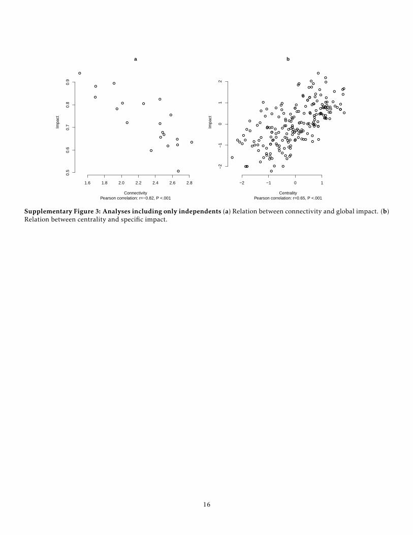
Future research might focus on how connectivity andcentrality of attitude networks relate to other factors that in-fluence voting decision. Among the most important factorsinfluencing voting decisions are party identification (Bartels,2000; Miller, 1991) and specific policy issues (Abramowitz,1995; Aldrich et al., 1989; Carmines & Stimson, 1980; Pal-frey & Poole, 1978; Nadeau & Lewis-Beck, 2001; Rabinowitz& MacDonald, 1989). First, party identification might in-fluence the connectivity of attitude networks, because it islikely that individuals, who identify with a political party,have a stronger drive for consistency in their attitudes to-ward presidential candidates. Party identification makes italso more likely that a given individual adopts a positive atti-tude toward the candidate of their party and it might also di-rectly influence the voting decision. This makes party iden-tification a possible confound of our results and we thereforealso ran our analyses including only individuals, who do notidentify with a political party. The results of this analysismirrored the results of the results reported in this paper (seeSupplementary Note 3 & Supplementary Figure 3). Second,policy issues might influence the centrality of attitude ele-ments. If, for example, the current political climate is highlyfocused on foreign policies (e.g., the conflict in Syria), judg-ing a candidate to be competent in respect to foreign policymaking might take a central place in the attitude network.Generally, it is an important question for future researchwhy some attitude elements are more central than others.Our analyses indicate that there are some attitude elementsthat are chronically central (see Figure 3), with some varia-tion that might be due to the specifics of the political climateduring the different elections.

Another promising venture for future research would beto investigate how attitude networks develop during an elec-tion campaign. To do so, one could apply several interme-diate assessments during the election campaign (Erikson &Wlezien, 1999; Taleb, 2017; Wlezien, 2003; Dalege, Bors-boom, van Harreveld, & van der Maas, 2017).The use of suchintermediate assessment was shown to improve the predic-tion of election outcomes (Taleb, 2017). How might attitudenetworks change during an election? Based on the CANmodel, we expect that (a) the connectivity of attitude net-works heighten during an election campaign and (b) attitudenetworks probably grow due to the addition of newly formedattitude elements (Dalege et al., 2016). Also, predictionsregarding the success of an election campaign to change agiven person’s attitude can be derived from the CAN model.

8

Individuals holding attitudes that are based on highly con-nected networks already at the beginning of an election cam-paign are likely to not change their attitudes. Election cam-paigns might thus benefit from focusing on individuals hold-ing attitudes that are based on weakly connected networks(Dalege et al., 2017).

In a broader sense, the CAN model advances our under-standing of the relation between attitudes and behaviouraldecisions. Because the CAN model is a general model of at-titudes, the results reported here likely generalize to otherattitudes and behavioural decisions than those studied hereas well. Using connectivity of attitude networks and cen-trality of attitude elements may for example provide moreinsight into issues such as which factors drive individualsto continue or stop smoking, buy a certain product, or be-have aggressively toward a minority group. Furthermore,connectivity of attitude networks might unify the differentapproaches to explain variations in attitude-behaviour con-sistency, as it is likely that network connectivity is the gluethat holds these factors together (Dalege et al., 2016) andbecause our results indicate that network connectivity com-prehensively explains variations in attitude-behaviour con-sistency. Several predictions above and beyond the findingsreported here can also be derived from the network structureof attitudes. For example, network structure predicts whenand which persuasion attempts will be successful (Dalege etal., 2016). Network theory thus holds great promise for ad-vancing our understanding of the dynamical and structuralproperties of attitudes and their relation to a plethora of con-sequential human behaviours.

MethodsSimulation of NetworksThe simulation of networks followed four steps. First, an un-weighted ’base’ network consisting of 11 variables was cre-ated based on preferential attachment (Barabasi & Albert,1999; Albert & Barabasi, 2002), the Small-World networkmodel (Watts & Strogatz, 1998), or the Erdos-Renyi randomgraph model (Erdos & Renyi, 1959) using the R packageiGraph (Csardi & Nepusz, 2006). The preferential attach-ment algorithm starts with one node and then adds one nodein each time step. The probability to which nodes the newnode connects depends on the degree of the old node:

Pr(i) =k(i)α + 1∑i k(j)α + 1

, (3)

where k(i) is the degree of a given node. α was set to varyuniformly between 0.30 and 0.70. At each time step m edgeswere added to the network. m was set to vary uniformly be-tween 4 and 6 (resulting in relatively dense networks, as wasshown to be the case for attitude networks, Dalege et al.,2016). The Small-World network model starts with a ringlattice with nodes being connected to n neighbours and then

randomly rewires edges with a p probability. n was set touniformly vary between 3 and 4 and p was set to uniformlyvary between 0.05 and 0.10. In the Erdos-Renyi graph, nodesare randomly connected by a given number of edges. Num-ber of edges was set to uniformly vary between 30 and 45.

Second, edge weights were added to the base network. Tohave psychometrically realistic edge weights, we drew edgeweights from either a normal distribution with M=0.15 andSD=.0075, a Pareto power law distribution with α=3 andβ=0.10, or a uniform distribution with range of 0.01–0.30.

Third, we created 20 variations of the weighted base net-work, in which the temperature of the Ising model was var-ied. The inverse temperature parameter β was drawn froma normal distribution with M=1 and SD=0.2 (with highernumbers representing low entropy). To ensure that all nodeshave roughly the same variance, we drew thresholds of nodesfrom a normal distribution with M=0 and SD=0.25.

Fourth, using the R-package IsingSampler (Epskamp etal., 2016), 1000 individuals for each of the variations of thebase network were simulated based on the probability dis-tribution implied by the Ising model. This procedure wasrepeated 900 times and each set of 20 variations of the dif-ferent 900 base networks was analysed separately.

ParticipantsThe open-access data of the ANES involves large nationalrandom probability samples. Data were each collected intwo interviews - one before and one after each presidentialelection from 1980 to 2012 - by the Center for Political Stud-ies of the University of Michigan. In total, 21,365 partic-ipants participated in these nine studies (for Ns per studysee Supplementary Table 2), of which 16,667 participantsstated that they voted for president. Non-voters were ex-cluded from the analyses, because we assume that the deci-sion whom to vote for is more likely to be part of the attitudenetwork than the decision whether to vote or not. In Supple-mentary Note 2, however, we show that similar findings areobtained when non-voters are included in the analysis.

MeasuresIn each of the studies between six and 16 items tapping be-liefs and between four and eight items tapping feelings to-ward the presidential candidates were assessed in the pre-election interviews. Feelings were assessed on two-pointscales and beliefs were assessed on four-point scales (in asubsample of the ANES of 2008 and in the ANES of 2012,beliefs were assessed on a five-point scale). To have compa-rable attitude networks between the different elections, wealways used six items tapping beliefs and four items tappingfeelings (see Table 1 for a list of included attitude elements).In the post-election interview, participants were asked whichcandidate they voted for. Depending on which presidentialcandidate the analysis focused, we scored the response as 1when the participant stated that they voted for the given can-didate and we scored the response as 0 when the participant

9

did not vote for the given candidate.

Statistical AnalysesWe performed the same statistical analyses on the simulatedand empirical data.Network EstimationAttitude networks were estimated using zero-order poly-choric (tetrachoric) correlations between the (simulated) at-titude elements as edge weights. We chose to use zero-order correlations as edge weights instead of estimating di-rect causal paths between the attitude elements because oursimulations have shown that attitude networks based onzero-order correlations perform better than techniques thatprovide an estimate of the underlying causal network (vanBorkulo et al., 2014).Network DescriptivesBoth the ASPL and closeness are based on shortest path be-tween lengths (d) between nodes. To calculate shortest pathlengths, we used Dijkstra’s algorithm (Dijkstra, 1959), im-plemented in the R package qgraph (Epskamp, Cramer, Wal-dorp, Schmittmann, & Borsboom, 2012):

dw(i, j) =min(1wih

+1whj

). (4)

ASPL is then the average of the shortest path lengths be-tween each pair of nodes in the network. Closeness (c) wascalculated using the algorithm for weighted networks devel-oped by Opsahl et al. (2010), using the R package qgraph:

c(i) =

N∑j

d(i, j)

−1

. (5)

Impact EstimatesTo estimate average impact of (simulated) attitude elementson (simulated) voting decisions, we calculated the biserialcorrelation between the sum score of (simulated) attitude el-ements and the (simulated) voting decision. We then calcu-lated the Pearson correlation between connectivity and aver-age impact for the 20 networks in the empirical study and foreach set of 20 variations of the base networks in the simula-tion study. The clearly linear relation between connectivityand impact justified the use of Pearson correlation and sig-nificance testing. For the simulation study, we calculated themean and standard deviation of the correlations obtained foreach set of variations of the base network.

To estimate the impact of a given (simulated) attitudeelement on the (simulated) voting decision, we calculatedthe zero-order polychoric correlation between a given (simu-lated) attitude element and the (simulated) voting decision.We then calculated the Pearson correlation between stan-dardized centrality and standardized impact of the attitudeelements in the empirical study and for each set of 20 vari-ations of the base networks in the simulation study. The

clearly linear relation between centrality and impact justi-fied the use of Pearson correlation and significance testing.For the simulation study, we calculated the mean and stan-dard deviation of the correlations obtained for each set ofvariations of the base network.

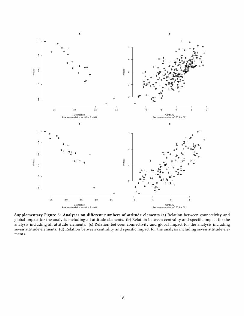
Forecast AnalysisFor the forecast analysis, we first conducted nine regressionanalyses, in which impact was regressed on centrality. Ineach regression analysis, the forecasted election was omitted.From each of the regression equations, we first extracted thebeta and intercept coefficients. Second, we multiplied thecentrality indices of the forecasted election with the beta co-efficient and added the intercept coefficient. Note that not inevery election the same attitude elements were assessed. Ofthe ten used attitude elements, seven were assessed at eachelection. For the remaining three, we grouped the attitudeelements together that were most similar to each other (seeTable 1). Third, we compared the resulting estimates withthe actual impact of the attitude elements and calculatedthe absolute deviance scores. We then compared the perfor-mance of the centrality prediction to the overall mean pre-diction and the specific mean prediction. For both these pre-dictions, we again calculated predictions nine times, omit-ting one of the elections each time. For the overall mean pre-diction, we calculated the mean of all attitude elements andfor the specific mean prediction, we calculated the mean ofeach specific attitude element. We tested whether the cen-trality prediction performed better than the overall meanprediction and the specific mean prediction using Wilcoxonsigned-rank tests.

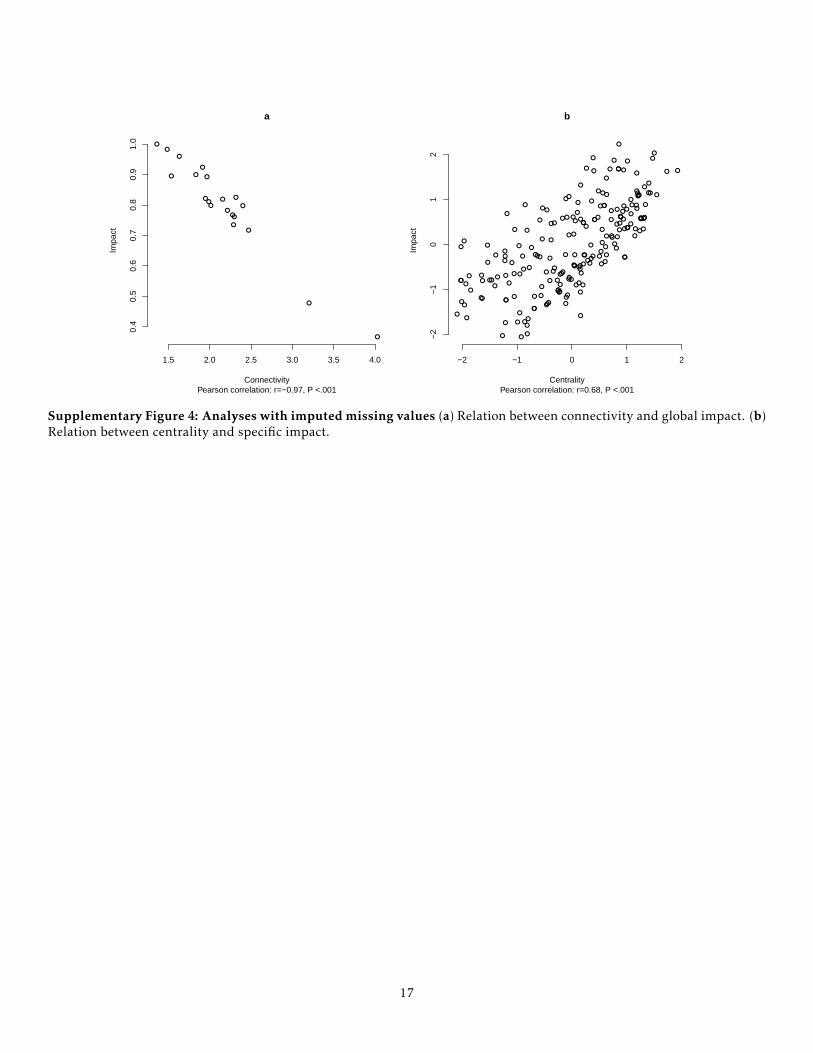
Missing ValuesMissing values were deleted casewise (Supplementary Table2 shows the number of excluded participants per attitudenetwork). Most missing values stemmed either from partici-pants responding to an item that they did not know the an-swer or from non-participation during the post-election in-terview. Few missing values stemmed from interview errors.

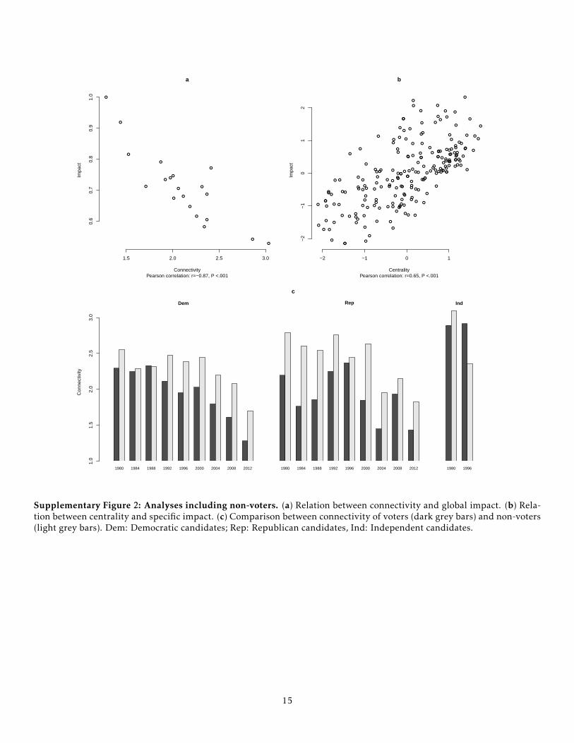
Alternative AnalysesWe also ran several alternative analyses that confirmed therobustness of our results: We ran alternative analyses onnon-voters (see Supplementary Note 2 & SupplementaryFigure 2), on independents (see Supplementary Note 3 &Supplementary Figure 3), on missing values (see Supple-mentary Note 4 & Supplementary Figure 4), on networkswith different number of nodes (see Supplementary Note 5& Supplementary Figure 5), and on latent variable models(see Supplementary Note 6 & Supplementary Table 3).

ReferencesAbramowitz, A. I. (1995). It’s abortion, stupid: Policy vot-

ing in the 1992 presidential election. Journal of Politics, 57,176–186.

10

Achen, C. (1975). Mass political attitudes and the survey re-sponse. American Political Science Review, 69, 1218–1231.

Ajzen, I. (1991). The theory of planned behavior. Organiza-tional Behavior and Human Decision Processes, 50, 179–211.

Ajzen, I., & Fishbein, M. (1977). Attitude-behavior relations:A theoretical analysis and review of empirical research.Psychological Bulletin, 84, 888–918.

Albert, R., & Barabasi, A.-L. (2002). Statistical mechanics ofcomplex networks. Review of Modern Physics, 74, 47–97.

Aldrich, J. H., Sullivan, J. L., & Borgida, E. (1989). Foreignaffairs and issue voting: Do presidential candidates ”waltzbefore a blind audience?”. American Political Science Re-view, 83, 123–141.

Ansolabehere, S., Rodden, J., & Snyder, J. M. (2008). Thestrength of issues: Using multiple measures to gauge pref-erence stability, ideological constraint, and issue voting.American Political Science Review, 102, 215–232.

Armitage, C. J., & Conner, M. (2000). Attitudinal ambiva-lence: A test of three key hypotheses. Personality and SocialPsychology Bulletin, 26, 1421–1432.

Bagozzi, R., & Baumgartner, J. (1986). The level of ef-fort required for behaviour as a moderator of the attitude-behaviour relation. European Journal of Social Psychology,20, 45–59.

Barabasi, A.-L. (2011). The network takeover. Nature Physics,8, 14–16.

Barabasi, A.-L., & Albert, R. (1999). Emergence of scaling inrandom networks. Science, 286, 509–512.

Barabasi, A.-L., & Zoltan, N. O. (2004). Network biology:Understanding the cell’s functional organization. NatureReview Genetics, 5, 101–113.

Bartels, L. M. (2000). Partisanship and voting behavior,1952-1996. American Journal of Political Science, 44, 35–50.

Besag, J. (1974). Spatial interaction and the statistical analy-sis of lattice systems. Journal of the Royal Statistical Society.Series B (Methodological), 36, 192–236.

Breckler, S. J. (1984). Empirical validation of affect, behavior,and cognition as distinct components of attitude. Journalof Personality and Social Psychology, 47, 1191–1205.

Brown, L. (1986). Fundamentals of statistical exponential fam-ilies. Hayward, CA:Institute of Mathematical Statistics.

Carmines, E., & Stimson, J. (1980). The two faces of issuevoting. American Political Science Review, 74, 78–91.

Chaiken, S., Pomerantz, E. M., & Giner-Sorolla, R. (1995).Structural consistency and attitude strength. In R. E. Petty& J. A. Krosnick (Eds.), Attitude strength: Antecedents andconsequences (pp. 387–412). Hillsdale, NJ: Lawrence Erl-baum.

Converse, P. E. (1970). Attitudes and non-attitudes: Con-tinuation of a dialogue. In E. R. Tufte (Ed.), The quanta-tive analysis of social problems (pp. 168–189). Reading, MA:Addison-Wesley.

Cramer, A. O. J., van der Sluis, S., Noordhof, A., Wichers, M.,Geschwind, N., Aggen, S. H., . . . Borsboom, D. (2012). Di-mensions of normal personality as networks in search ofequilibrium: You can’t like parties if you don’t like people.European Journal of Personality, 26, 414–431.

Cramer, A. O. J., Waldorp, L. J., van der Maas, H. L. J., &Borsboom, D. (2010). Comorbidity: A network perspec-tive. Behavioral and Brain Sciences, 33, 137–193.

Csardi, G., & Nepusz, T. (2006). The igraph software pack-age for complex network research. InterJournal ComplexSystems, 1695.

Dalege, J., Borsboom, D., van Harreveld, F., van den Berg,H., Conner, M., & van der Maas, H. L. J. (2016). Toward aformalized account of attitudes: The Causal Attitude Net-work (CAN) model. Psychological Review, 123, 2–22.

Dalege, J., Borsboom, D., van Harreveld, F., & van derMaas, H. L. J. (2017). A network perspective onpolitical attitudes: Testing the connectivity hypothesis.(https://arxiv.org/abs/1705.00193)

Dijkstra, E. W. (1959). A note on two problems in connexionwith graphs. Numerische Mathematik, 1, 269–271.

Eagly, A. H., & Chaiken, S. (1993). The psychology of attitudes.Orlando, FL: Harcourt Brace Jovanovich.

Epskamp, S., Cramer, A. O. J., Waldorp, L. J., Schmittmann,V. D., & Borsboom, D. (2012). qgraph: Network visual-izations of relationships in psychometric data. Journal ofStatistical Software, 48, 1–18.

Epskamp, S., Maris, G., Waldorp, L., & Borsboom,D. (2016). Network psychometrics. (Preprint athttps://arxiv.org/abs/1609.02818)

Erdos, P., & Renyi, A. (1959). On random graphs. Publica-tiones Mathematicae, 6, 290–297.

Erikson, R. S., & Wlezien, C. (1999). Presidential polls asa time series: The case of 1996. Public Opinion Quarterly,63, 163–177.

Fazio, R. H. (1995). Attitudes as object-evaluation associa-tions: Determinants, consequences, and correlates of atti-tude accessibility. In R. E. Petty & J. A. Krosnick (Eds.),Attitude strength: Antecedents and consequences (pp. 247–282). Hillsdale, NJ: Lawrence Erlbaum.

Fazio, R. H., & Williams, C. J. (1986). Attitude accessibil-ity as a moderator of the attitude-perception and attitude-behavior relations: An investigation of the 1984 presiden-tial election. Journal of Personality and Social Psychology,51, 505–514.

Fazio, R. H., & Zanna, M. (1981). Direct experience andattitude-behavior consistency. Advances in ExperimentalSocial Psychology, 14, 161–202.

Fishbein, M., & Ajzen, I. (1975). Belief, attitude, intention andbehavior: An introduction to theory and research. Reading,MA: Addison-Wesley.

Freeman, L. C. (1978). Centrality in social networks: Con-ceptual clarification. Social Networks, 1, 215–239.

Fruchterman, T., & Reingold, E. (1991). Graph drawing by

11

force directed placement. Software, Practice & Experience,21, 1129–1164.

Galdi, S., Arcuri, L., & Gawronski, B. (2008). Automaticmental associations predict future choices of undecideddecision-makers. Science, 321, 1100–1102.

Glasman, L. R., & Albarracın, D. (2006). Forming atti-tudes that predict future behavior: A meta-analysis ofthe attitude-behavior relation. Psychological Bulletin, 132,778–822.

Hastie, T., Tibshirani, R., & Friedman, J. (2001). The elementsof statistical learning. New York, NY: Springer.

Hastie, T., Tibshirani, R., & Wainwright, M. (2015). Statisti-cal learning with sparsity: The lasso and generalizations. NewYork, NY: CRC Press.

Ising, E. (1925). Beitrag zur Theorie des Ferromagnetismus.Zeitschrift fur Physik, 31, 253–258.

Jacoby, W. G. (2010). Policy attitudes, ideology and votingbehavior in the 2008 election. Electoral Studies, 29, 557–568.

Judd, C., & Krosnick, J. (1989). The structural bases ofconsistency among political attitudes: Effects of expertiseand attitude importance. In A. Pratkanis, S. Breckler, &A. Greenwald (Eds.), Attitude structure and function (pp.99–128). Hillsdale, NJ: Lawrence Erlbaum.

Judd, C., Krosnick, J., & Milburn, M. (1980). The structureof attitude systems in the general public: Comparisons ofa structural equation model. American Sociological Review,45, 627–643.

Judd, C., Krosnick, J., & Milburn, M. (1981). Political in-volvement and attitude structure in the general public.American Sociological Review, 46, 660–669.

Kolaczyk, E. D. (2009). Statistical analysis of network data:Methods and models. New York, NY: Springer.

Kraus, S. J. (1986). Attitudes and the prediction of behavior:A meta-analysis of the empirical literature. Personality andSocial Psychology Bulletin, 51, 505–514.

Krosnick, J. A. (1988). The role of attitude importance insocial evaluation: a study of policy preferences, presiden-tial candidate evaluations, and voting behavior. Journal ofPersonality and Social Psychology, 55, 196–210.

Krosnick, J. A. (1989). Attitude importance and attitude ac-cessibility. Personality and Social Psychology Bulletin, 15,297–308.

Krosnick, J. A., Boninger, D. S., Chuang, Y. C., Berent, M. K.,& Carnot, C. G. (1993). Attitude strength: One constructor many related constructs? Journal of Personality and So-cial Psychology, 65, 1132–1151.

Krosnick, J. A., & Petty, R. E. (1995). Attitude strength: Anoverview. In R. E. Petty & J. A. Krosnick (Eds.), Attitudestrength: Antecedents and consequences (pp. 1–24). Hills-dale, NJ: Lawrence Erlbaum.

Kruglanski, A. W., Katarzyna, J., Chernikova, M., Milyavsky,M., Babush, M., Baldner, C., & Pierro, A. (2015). The rockyroad from attitudes to behaviors: Charting the goal sys-

temic course of actions. Psychological Review, 122, 598–620.

LaPiere, E. (1934). Attitudes vs. actions. Social Forces, 13,230–237.

Lavine, H., Thomsen, C. J., Zanna, M. P., & Borgida, E.(1998). On the primacy of affect in the determination ofattitudes and behavior: The moderating role of affective-cognitive ambivalence. Journal of Experimental Social Psy-chology, 34, 398–421.

Little, R. J. A. (1988). Missing-data adjustments in large sur-veys. Journal of Business & Economic Statistics, 6, 287–296.

Markus, G. B. (1982). Political attitudes during an electionyear: A report on the 1980 nes panel study. American Po-litical Science Review, 76, 538–560.

Millar, M. G., & Millar, K. U. (1996). Affective and cogni-tive responses and the attitude-behavior relation. Journalof Experimental Social Psychology, 32, 561–579.

Miller, W. E. (1991). Party identification, realignment , andparty voting: Back to the basics. American Political ScienceReview, 85, 557–568.

Monroe, B. M., & Read, S. J. (2008). A general connection-ist model of attitude structure and change: the ACS (Atti-tudes as Constraint Satisfaction) model. Psychological Re-view, 115, 733–759.

Murphy, K. (2012). Machine learning: A probabilistic perspec-tive. Cambridge, MA: MIT Press.

Nadeau, R., & Lewis-Beck, M. S. (2001). National economicvoting in U.S. presidential elections. Journal of Politics, 63,159–181.

Newman, M. E. J. (2010). Networks: An introduction. Oxford:Oxford University Press.

Opsahl, T., Agneessens, F., & Skvoretz, J. (2010). Nodecentrality in weighted networks: Generalizing degree andshortest paths. Social Networks, 32, 245–251.

Palfrey, T. R., & Poole, K. T. (1978). Economic retrospectivevoting in American national elections: A micro-analysis.American Journal of Political Science, 22, 426–443.

Palfrey, T. R., & Poole, K. T. (1987). The relationship betweeninformation, ideology, and voting behavior. American Jour-nal of Political Science, 31, 511–530.

Rabinowitz, G., & MacDonald, S. E. (1989). A directionaltheory of issue voting. American Political Science Review,83, 93–121.

Rosenberg, M. J., Hovland, C. I., McGuire, R. P., W.J.and Abelson, & Brehm, J. W. (1960). Attitude organi-zation and change: An analysis of consistency among attitudecomponents. New Haven, CA: Yale University Press.

Taleb, N. (2017). How to forecast an election.(https://arxiv.org/abs/1703.06351)

Thompson, M. M., Zanna, M. P., & Griffin, D. W. (1995).Let’s not be indifferent about (attitudinal) ambivalence. InR. E. Petty & J. A. Krosnick (Eds.), Attitude strength: An-tecedents and consequences (pp. 361–386). Hillsdale, NJ:Lawrence Erlbaum.

12

van Borkulo, C. D., Borsboom, D., Epskamp, S., Blanken,B. W., Bosschloo, L., Schoevers, R. A., & Waldorp, L. J.(2014). A new method for constructing networks from bi-nary data. Scientific Reports, 4, 5918.

van Borkulo, C. D., Boschloo, L., Borsboom, D., Penninx,B. W. J. H., Waldorp, L. J., & Schoevers, R. A. (2015). Asso-ciation of symptom network structure with the course ofdepression. JAMA Psychiatry, 72, 1219–1226.

van Buuren, S., & Groothuis-Oudshoorn, K. (2011). Multi-variate imputation by chained equations. Journal of Statis-tical Software, 45, 1–67.

van de Leemput, I. A., Wichers, M., Cramer, A. O. J., Bors-boom, D., Tuerlinckx, F., Kuppens, P., . . . Scheffer, M.(2014). Critical slowing down as early warning for the on-set and termination of depression. Proceedings of the Na-tional Academy of Sciences of the United States of America,111, 87–92.

van den Berg, H., Manstead, A. S. R., van der Pligt, J., & Wig-boldus, D. H. J. (2005). The role of affect in attitudes to-ward organ donation and donor-relevant decisions. Psy-chology and Health, 20, 789–802.

van der Pligt, J., de Vries, N. K., Manstead, A. S. R., & vanHarreveld, F. (2000). The importance of being selective:Weighing the role of attribute importance. Advances in Ex-perimental Social Psychology, 32, 135–200.

van Harreveld, F., Nohlen, H. U., & Schneider, I. K. (2015).The abc of ambivalence: Affective, behavioral, and cogni-tive consequences of attitudinal conflict. Advances in Ex-perimental Social Psychology, 52, 285–324.

van Harreveld, F., van der Pligt, J., de Vries, N. K., & Andreas,S. (2000). The structure of attitudes: attribute importance,accessibility and judgment. British Journal of Social Psy-chology, 39, 363–380.

Visser, P. S., Bizer, G., & Krosnick, J. A. (2006). Exploringthe latent structure of strength-related attitude attributes.Advances in Experimental Social Psychology, 38, 1–67.

Visser, P. S., Krosnick, J. A., & Simmons, J. P. (2003). Distin-guishing the cognitive and behavioral consequences of at-titude importance and certainty: A new approach to test-ing the common-factor hypothesis. Journal of ExperimentalSocial Psychology, 39, 118–141.

Wainwright, M. J., & Jordan, M. I. (2008). Graphical models,exponential families, and variational inference. Founda-tions and Trends®in Machine Learning, 1, 1–305.

Wallis, W. D. (2007). A beginner’s guide to graph theory. NewYork, NY: Birkhauser.

Watts, D. J., & Strogatz, S. H. (1998). Collective dynamics of‘small-world’ networks. Nature, 393, 440–442.

West, D. B. (1996). Introduction to graph theory. Upper SaddleRiver, NJ: Prentice Hall.

Wicker, A. W. (1969). Attitudes versus actions: The relation-ship of verbal and overt behavioral responses to attitudeobjects. Journal of Social Issues, 25, 41–78.

Wlezien, C. (2003). Presidential election polls in 2000: Astudy in dynamics. Presidential Studies Quarterly, 33, 172–186.

Young, G., & Smith, R. (2005). Essentials of statistical infer-ence. Cambridge, UK: Cambridge University Press.

Zanna, M. P., & Rempel, J. K. (1988). Attitudes: A new lookat an old concept. In D. Bar-Tal & A. W. Kruglanski (Eds.),The psychology of knowledge (pp. 315–334). Cambridge,UK: Cambridge University Press.

AcknowledgementsWe thank S. Epskamp and G. Costantini for help with thesimulation studies; M. Deserno for help with the data anal-yses. D. B. was supported by a Consolidator Grant No.647209 from the European Research Council.

Author ContributionsJ.D. developed the study concept; J.D., D.B., F.v.H., andH.L.J.v.d.M contributed to the study design; J. D. performedthe data analysis and interpretation under the supervisionof D.B., F.v.H., and H.L.J.v.d.M.; J.D. drafted the manuscript,and D.B., F.v.H., and H.L.J.v.d.M. provided critical revisions.L.J.W. provided the analytical solutions of the hypotheses.

Author InformationData used in this paper is available at www.electionstudies.org.Correspondence and request for materials should be ad-dressed to J.D. ([email protected]).

Competing Financial InterestThe authors declare no competing financial interests.

13

Supplementary Materials for: Network Structure Explains theImpact of Attitudes on Voting DecisionsJonas Dalege, Denny Borsboom, Frenk van Harreveld, Lourens J. Waldorp & Han L. J. van der Maas

Department of Psychology, University of Amsterdam, 1018 WT Amsterdam, The Netherlands

Supplementary Figures

-4 -2 0 2 4

01

23

45

6

zµ

loss

log2(1 + exp(−zµ))

1(zµ < 0)

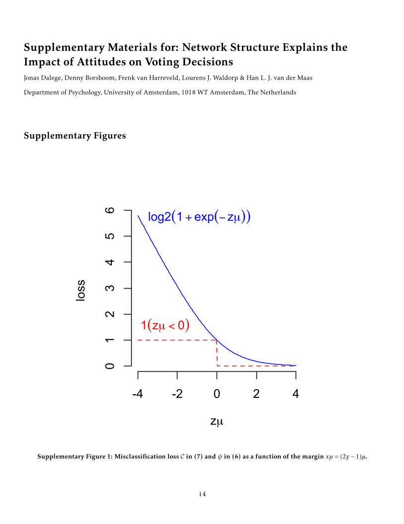
Supplementary Figure 1: Misclassification loss C in (7) and ψ in (6) as a function of the margin xµ = (2y − 1)µ.

14

●

●

●

●

●

●

●

●

●

●

●

●

●

●

●

●

●

●

●

●

1.5 2.0 2.5 3.0

0.6

0.7

0.8

0.9

1.0

Connectivity

Impa

cta

Pearson correlation: r=−0.87, P <.001

●

●

●

●

●

●

●

●

●

●

●

●

●

●

● ●

●

●

●

●

●●

●

●

●

●

●

●

●

●

●

●

●

●

●●

●

●

●●

●

●

●

●

●

●

●

●

●

●

●

●

●

●

●

●

●

●

● ●

●

●

●

●●

●

●

●

●

●

●

●

●

●

●

●

●

●

●

●

●

●

●

●

●

●

●

●

●

●

●

●

●

●

●

●

●

●

●

● ●

●●

●

●

●

●

●

●

● ●

●

●

●

●●

●

●

●

●

●

●●

●

●

●

●

●

●

●●

●

●

●

●

●

●

●

●

● ●

●

●

●

● ●

●

●

●

●

●

●

●

●

●

●

●

●

●

● ●

●

●

●

●

●

●

●

●

●

●

●

●

●

●

●

●

●

●

●

●

●●

●

●

●

●

●

●

●

●

●

●

●

●

●

●

●

●

●

●

●

●

●

●

●

●

●

●

●

−2 −1 0 1

−2

−1

01

2

Centrality

Impa

ct

b

Pearson correlation: r=0.65, P <.001

Con

nect

ivity

1.0

1.5

2.0

2.5

3.0

c

Dem Rep Ind

1980 1984 1988 1992 1996 2000 2004 2008 2012 1980 1984 1988 1992 1996 2000 2004 2008 2012 1980 1996

Supplementary Figure 2: Analyses including non-voters. (a) Relation between connectivity and global impact. (b) Rela-tion between centrality and specific impact. (c) Comparison between connectivity of voters (dark grey bars) and non-voters(light grey bars). Dem: Democratic candidates; Rep: Republican candidates, Ind: Independent candidates.

15

●

●

●

●

●

●

● ●

●

●

●

●●

●

●

●

●

●

●

●

1.6 1.8 2.0 2.2 2.4 2.6 2.8

0.5

0.6

0.7

0.8

0.9

Connectivity

Impa

cta


●

●

●

●

●

●

●

●

●

●

●

●

●

●

●

●

● ●

●

●

●●

●

●

●

●

●

●

●

●

●

●

●

●

●

●

●

●

●

●

●

●

●

●

●

●

●

●

●

●

●

●

●

●●

●

●

●

●

●

●●

●

●

●

●●

●

●

●

●

●

●

●

●

●

●

●

●● ●

●

●

●

●

●

●●

●

●

● ●

●

●

●

●

●

●

●

●

●

●

● ●

●

●●

●

●

●

● ●

●

●

●

●

●

●

●

●

●

●

● ●

●

●●

●

●

●

●

●

●

●

●

●

●

●

●

●

●

●

●

●

●

●

●

●

●

●

●

●

●

●

●

●

●

●

● ●

●

●

●

●

●

●

●

●

●

●

●

●

●

●

●

●

●

●

●

●

●

●

●

●

●

●

●

●

●

●

●

●

●

●

●

●

●

●●

●

●

●

●

●

●

●

●

●

●

●

−2 −1 0 1

−2

−1

01

2

Centrality

Impa

ct

b


Supplementary Figure 3: Analyses including only independents (a) Relation between connectivity and global impact. (b)Relation between centrality and specific impact.

16

●

●

●

●

●

●

●

●●

●

●

●

●●

●

●

●

●

●

●

1.5 2.0 2.5 3.0 3.5 4.0

0.4

0.5

0.6

0.7

0.8

0.9

1.0

Connectivity

Impa

cta


●

●

●

●

●

●

●●

●

●

●

●

●

●

●

●

●

●

●

●

●

●

●

●

●

●

●

●

●

●

●

●

●

●

●

●

●

●

●

●

●

●

●

●

●

●

●

●

●

●

●●

●

●

●

●

●

●

●●

●

●

●

●

●●

●

●

●

●

●

●

●

●

●

●

●

●

●

●

●

●

●

● ●

●

●●

●

●

●

●

●

●

●

●

●

●

●

●

●

●

●

●

●

●

●

●

●

●●

●

●

● ●●

●

●

●

●

●

●

●

●

●

●

●

●

●

●

●

●

●

●

●

●

●

●

● ●

●

●

●

●

●

●

●

●

●

●

●

●

●

●

●

●

●

●

●

●

●

●

●

●

●

●

●

●

●

●

●

●

●

●

●

●

●

●

●

●

●

●

●

●

●

●

●

●

●

●

●

●

●

●

●

●

●

●

●

●

●

●

●

●

●

●

●

●

●

●

−2 −1 0 1 2

−2

−1

01

2

Centrality

Impa

ct

b


Supplementary Figure 4: Analyses with imputed missing values (a) Relation between connectivity and global impact. (b)Relation between centrality and specific impact.

17

●

●

●

●

●

●

●

●

●

●

●

●●

●

●

●

●

●

●

●

1.5 2.0 2.5 3.0

0.6

0.7

0.8

0.9

1.0

Connectivity

Impa

cta


●

●

●

●

●

●

● ●

●

●

●

●

●

●

●

●

●

●●

●

●

●

●

●

●

●

●

●

●●

●

●

●

●

●

●

●

●

●

●

●

●

●

●

●

●

●

●

●

●

●●

●

●●

●

●

●●

●

●●

●

●

●

●

●●

●

●

●

●

●

●

●●

●

●

●

●

●

●

●

●●

●

●

●

●

●

●

●

●

●

●

●

●

●

●

●

●

●

●

●

●

●

●

●

●

●

●

●

●

●

●

●

●

●

●

●

●

●

●

●

●

●

●●

●

●

●

●

●

●

●●

●

●

●

●

●●

●

●

●

●

●

●

●

●

●

●

●

●

●

●

● ●

●

●

●

●

●

●

●

●

●

●

●

●

●

●●

●●

●

●

●

●

●

●

●

●

●

●

●

●

●

●●

●

●

●

●

●

●

●

●

●

●

●

●

●

●

●

●

●

●

●

●

●

●

●

●●

●

●

●

●

●

●

●

●

●

●

●

●

●

●

●

●

●

●

●

●

●

●

●

●

●

●

●

●

●

●

●

●

●

●

●

●

●

●

●

●

●

●

●

●

●

●

●

●

●

●

−2 −1 0 1 2

−2

−1

01

2

Centrality

Impa

ct

b


●

●

●●

●

●

●●

●

●

●

●

●●

●

●

●

●

●

●

1.5 2.0 2.5 3.0 3.5

0.5

0.6

0.7

0.8

0.9

1.0

Connectivity

Impa

ct

c


●

●

●

●

●

●

●

●

●

●

●

●

●

●

●

●

●

●

●

●

●

●

●

●

●

●

●●

●

●

●

●

●

●

●

●

●

●

●

●

●

●

●

●

●

●

●

●

●

●

●

●

●

●

●

●

●

●

●

●●

●

●

●

●

●

●

●

●

●

●

●

●

●

●

●

●●

●

●

●

●

●

●

●

●

●

●

●

●

●

●

●

●

●

●

●●

●

●

●

●

●

●

●

●

●

●

●

●

●●

●

●

●

●

●

●

●

●

●

●

●

●

●

●

●

●

●

●

●

●

●

●

●

●

●

●

●

●

●

●

●

●

●

●

●

−2 −1 0 1

−1

01

2

Centrality

Impa

ctd


Supplementary Figure 5: Analyses on different numbers of attitude elements (a) Relation between connectivity andglobal impact for the analysis including all attitude elements. (b) Relation between centrality and specific impact for theanalysis including all attitude elements. (c) Relation between connectivity and global impact for the analysis includingseven attitude elements. (d) Relation between centrality and specific impact for the analysis including seven attitude ele-ments.

18

Supplementary Tables

Supplementary Table 1: Results of the Simulations for Each Network-Generating Algorithm and Edge Weight Distri-bution.

Preferential attachment Small-world Random graphConnectivity/impact correlations

Normal distribution mean r=-0.91 mean r=-0.91 mean r=-0.90s.d. r=0.07 s.d. r=0.05 s.d. r=0.08

Power-law distribution mean r=-0.92 mean r=-0.91 mean r=-0.91s.d. r=0.05 s.d. r=0.05 s.d. r=0.04

Uniform distribution mean r=-0.92 mean r=-0.89 mean r=-0.90s.d. r=0.05 s.d. r=0.08 s.d. r=0.08Centrality/impact correlations

Normal distribution mean r=0.72 mean r=0.51 mean r=0.57s.d. r=0.18 s.d. r=0.33 s.d. r=0.27

Power-law distribution mean r=0.70 mean r=0.46 mean r=0.60s.d. r=0.19 s.d. r=0.34 s.d. r=0.23

Uniform distribution mean r=0.68 mean r=0.49 mean r=0.60s.d. r=0.24 s.d. r=0.29 s.d. r=0.25

19

Supplementary Table 2: Number of participants per election and number of participants with missing values.

Election N complete sample N non-voters N missing values Democratic candidates) N missing values (Republican candidates)

1980 1,614 411 338 396

1984 2,257 539 583 435

1988 2,040 545 470 477

1992 2,485 562 567 358

1996 1,714* 374 239 318

2000 1,807 376 440 493

2004 1,212 231 282 195

2008 2,322 509 368 390

2012 5,914 1,141 557 644

Note. *Of these 1,714 participants, 1,316 participants also participated during the election of 1992.

20

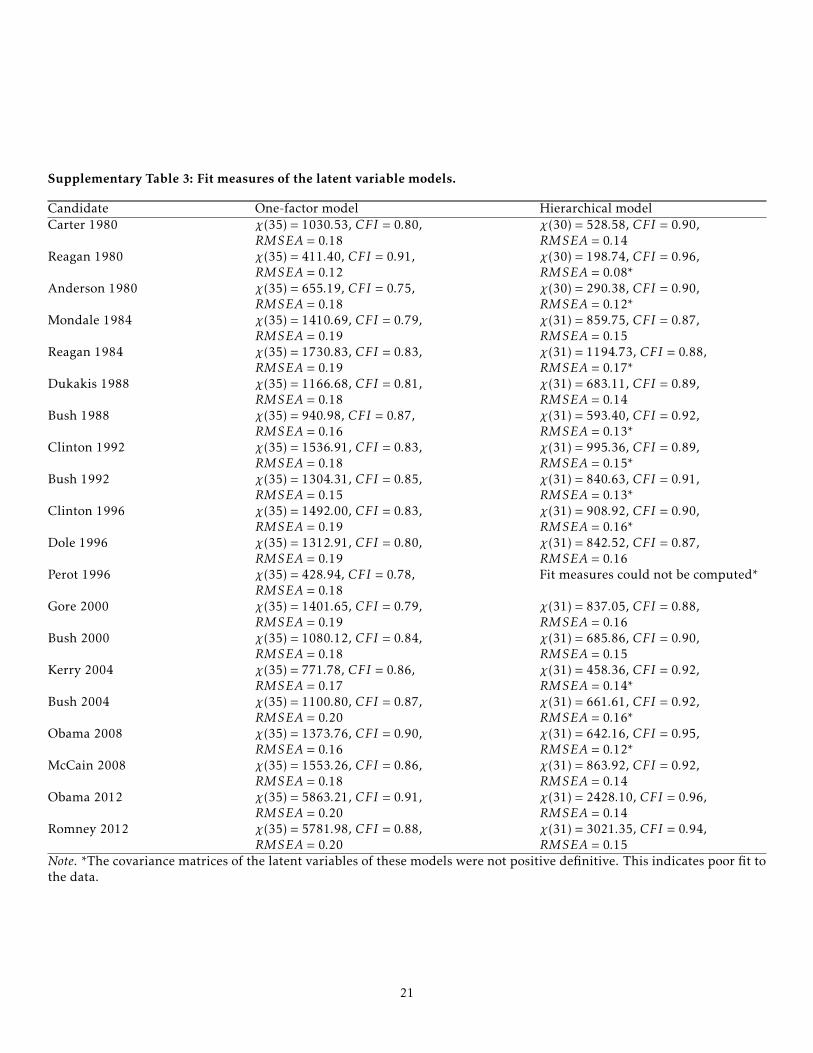
Supplementary Table 3: Fit measures of the latent variable models.

Candidate One-factor model Hierarchical modelCarter 1980 χ(35) = 1030.53, CFI = 0.80, χ(30) = 528.58, CFI = 0.90,

RMSEA = 0.18 RMSEA = 0.14Reagan 1980 χ(35) = 411.40, CFI = 0.91, χ(30) = 198.74, CFI = 0.96,

RMSEA = 0.12 RMSEA = 0.08*Anderson 1980 χ(35) = 655.19, CFI = 0.75, χ(30) = 290.38, CFI = 0.90,

RMSEA = 0.18 RMSEA = 0.12*Mondale 1984 χ(35) = 1410.69, CFI = 0.79, χ(31) = 859.75, CFI = 0.87,

RMSEA = 0.19 RMSEA = 0.15Reagan 1984 χ(35) = 1730.83, CFI = 0.83, χ(31) = 1194.73, CFI = 0.88,

RMSEA = 0.19 RMSEA = 0.17*Dukakis 1988 χ(35) = 1166.68, CFI = 0.81, χ(31) = 683.11, CFI = 0.89,

RMSEA = 0.18 RMSEA = 0.14Bush 1988 χ(35) = 940.98, CFI = 0.87, χ(31) = 593.40, CFI = 0.92,

RMSEA = 0.16 RMSEA = 0.13*Clinton 1992 χ(35) = 1536.91, CFI = 0.83, χ(31) = 995.36, CFI = 0.89,

RMSEA = 0.18 RMSEA = 0.15*Bush 1992 χ(35) = 1304.31, CFI = 0.85, χ(31) = 840.63, CFI = 0.91,

RMSEA = 0.15 RMSEA = 0.13*Clinton 1996 χ(35) = 1492.00, CFI = 0.83, χ(31) = 908.92, CFI = 0.90,

RMSEA = 0.19 RMSEA = 0.16*Dole 1996 χ(35) = 1312.91, CFI = 0.80, χ(31) = 842.52, CFI = 0.87,

RMSEA = 0.19 RMSEA = 0.16Perot 1996 χ(35) = 428.94, CFI = 0.78, Fit measures could not be computed*

RMSEA = 0.18Gore 2000 χ(35) = 1401.65, CFI = 0.79, χ(31) = 837.05, CFI = 0.88,

RMSEA = 0.19 RMSEA = 0.16Bush 2000 χ(35) = 1080.12, CFI = 0.84, χ(31) = 685.86, CFI = 0.90,

RMSEA = 0.18 RMSEA = 0.15Kerry 2004 χ(35) = 771.78, CFI = 0.86, χ(31) = 458.36, CFI = 0.92,

RMSEA = 0.17 RMSEA = 0.14*Bush 2004 χ(35) = 1100.80, CFI = 0.87, χ(31) = 661.61, CFI = 0.92,

RMSEA = 0.20 RMSEA = 0.16*Obama 2008 χ(35) = 1373.76, CFI = 0.90, χ(31) = 642.16, CFI = 0.95,

RMSEA = 0.16 RMSEA = 0.12*McCain 2008 χ(35) = 1553.26, CFI = 0.86, χ(31) = 863.92, CFI = 0.92,

RMSEA = 0.18 RMSEA = 0.14Obama 2012 χ(35) = 5863.21, CFI = 0.91, χ(31) = 2428.10, CFI = 0.96,

RMSEA = 0.20 RMSEA = 0.14Romney 2012 χ(35) = 5781.98, CFI = 0.88, χ(31) = 3021.35, CFI = 0.94,

RMSEA = 0.20 RMSEA = 0.15Note. *The covariance matrices of the latent variables of these models were not positive definitive. This indicates poor fit tothe data.

21

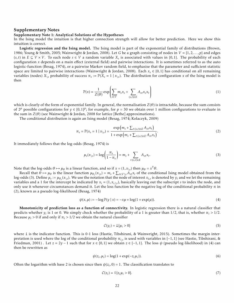
Supplementary NotesSupplementary Note 1: Analytical Solutions of the HypothesesIn the Ising model the intuition is that higher connection strength will allow for better prediction. Here we show thisintuition is correct.

Logistic regression and the Ising model. The Ising model is part of the exponential family of distributions (Brown,1986; Young & Smith, 2005; Wainwright & Jordan, 2008). Let G be a graph consisting of nodes in V = {1,2, . . . ,p} and edges(s, t) in E ⊆ V × V . To each node s ∈ V a random variable Xs is associated with values in {0,1}. The probability of eachconfiguration x depends on a main effect (external field) and pairwise interactions. It is sometimes referred to as the autologistic-function (Besag, 1974), or a pairwise Markov random field, to emphasise that the parameter and sufficient statisticspace are limited to pairwise interactions (Wainwright & Jordan, 2008). Each xs ∈ {0,1} has conditional on all remainingvariables (nodes) X\s probability of success πs := P(Xs = 1 | x\s). The distribution for configuration x of the Ising model isthen

P(x) =1

Z(θ)exp

∑s∈V

msxs +∑

(s,t)∈EAstxsxt

(1)

which is clearly of the form of exponential family. In general, the normalisation Z(θ) is intractable, because the sum consistsof 2p possible configurations for y ∈ {0,1}p; for example, for p = 30 we obtain over 1 million configurations to evaluate inthe sum in Z(θ) (see Wainwright & Jordan, 2008 for lattice [Bethe] approximations).

The conditional distribution is again an Ising model (Besag, 1974; Kolaczyk, 2009)

πs = P(xs = 1 | x\s) =exp

(ms +

∑t:(s,t)∈EAstxt

)1 + exp

(ms +

∑t:(s,t)∈EAstxt

) . (2)

It immediately follows that the log-odds (Besag, 1974) is

µs(x\s) = log(πs

1−πs

)=ms +

∑t:(s,t)∈E

Astxt . (3)

Note that the log-odds θ 7→ µθ is a linear function, and so if x = (1,x\s) then µθ = xTθ.Recall that θ 7→ µθ is the linear function µθs (x\s) = ms +

∑t∈V \sAstxt of the conditional Ising model obtained from the

log-odds (3). Define µs := µθs (x\s). We use the notation that the node of interest xi,s is denoted by yi and we let the remainingvariables and a 1 for the intercept be indicated by xi = (1,xi,\s), basically leaving out the subscript s to index the node, andonly use it whenever circumstances demand it. Let the loss function be the negative log of the conditional probability π in(2), known as a pseudo log-likelihood (Besag, 1974)

ψ(x,µ) := − logP(y | x) = −xµ+ log(1 + exp(µ)). (4)

Monotonicity of prediction loss as a function of connectivity. In logistic regression there is a natural classifier thatpredicts whether yi is 1 or 0. We simply check whether the probability of a 1 is greater than 1/2, that is, whether πi > 1/2.Because µi > 0 if and only if πi > 1/2 we obtain the natural classifier

C(yi) = 1{µi > 0} (5)

where 1 is the indicator function. This is 0-1 loss (Hastie, Tibshirani, & Wainwright, 2015). Sometimes the margin inter-pretation is used where the log of the conditional probability πi,s is used with variables in {−1,1} (see Hastie, Tibshirani, &Friedman, 2001) . Let z = 2y − 1 such that for x ∈ {0,1} we obtain z ∈ {−1,1}. The loss ψ (pseudo log-likelihood) in (4) canthen be rewritten as

ψ(zi ,µi) = log(1 + exp(−ziµi)). (6)

Often the logarithm with base 2 is chosen since then ψ(zi ,0) = 1. The classification translates to

C(zi) = 1{ziµi > 0}. (7)

22

Logistic loss ψ in (6) is an upper bound to C in (7), and is 1 at the value of the margin ziµi = 0, as shown in SupplementaryFigure 1. Here we use logistic loss ψ as defined in (4) because it is more common. This function is strictly monotonedecreasing.

It follows immediately from monotonicity that ψ(zi ,µ) > ψ(zi ,µ∗) if µ < µ∗. Of course, we have the same for the 0-1 loss:1{ziµi > 0} ≥ 1{ziµ∗i > 0} if µ < µ∗.

If the average degree of each node were subtracted from the Hamiltonian µs, then we obtain the Ising model without anexternal field. If we have

ms = −12

∑t:(s,t)∈E

Ast (8)

then we see thatµs = −1

2

∑t:(s,t)∈E

Ast +∑

t:(s,t)∈EAstxsxt =

∑t:(s,t)∈E

Ast(xsxt − 1/2) (9)

to the labeling z = 2y − 1 ∈ {−1,1}, we obtain that the average is 0 (implying ms = 0), and so the Hamiltonian consists onlyof the interactions

∑t:(s,t)∈EAstzszt . And so if Ast ≥ 0 for all s, t ∈ V then µ∗s > µs iff A∗st > Ast , i.e., the Hamiltonian is larger if

and only of the connectivity is larger. As seen above, this leads immediately to the monotonicity above.Closeness and correlations Let dst(r) = min{1/rsi + 1/rij + · · · + 1/rkt : ∀i, j,k ∈ V \{s, t}} be the shortest distance in terms

of Dijkstra’s algorithm (Wallis, 2007), where rij is the weight, in our case a (polychromic) correlation that are all positive.Then closeness is defined as

cs(r) =

∑t∈V \{s}

dst(r)

−1

(10)

The intuition is here that a node with high closeness will have connections or paths to other nodes with high correlations(weights). To see the intuition, consider node s being connected only to node t with correlation rst . Then cs(r) = rst ; if thiscorrelation is high, then so is the closeness of this node. If there is more than one connection, we see that the shortest pathdst(r) is low if all correlations rij are high (close to 1), implying that closeness cs(r) is high.

Suppose we have two sets weights R1 and R2, inducing two graphs G1 and G2 with the same nodes and edge sets butwith different weights. We pick a path between nodes s and t, denoted by Pst = {(x0 = s,x1), (x1,x2), . . . , (xk−1,xk = t)} of lengthk. Suppose that for this path we have

k∑i=0

r1,i−1,i ≥k∑i=0

r2,i−1,i (11)

Then it follows thatk∑i=0

1r1,i−1,i

≤k∑i=0

1r2,i−1,i

(12)

In other words, the higher the correlations the higher the closeness. This does not imply that any randomly drawn nodeconnected to a node with high closeness will have a high correlation, only that on average the correlations will be higher ifthey are connected to a node with high closeness than if they are connected to a node with low closeness.Supplementary Note 2: Alternative Analysis on Non-VotersTo investigate whether our results are robust to the inclusion of non-voters, we performed the same analyses but nowincluding non-voters and labelling them as voters against the focal candidates. The results of this analysis mirrored theresults reported in the Results section: The correlation between connectivity and average impact remained high and signif-icant (see Supplementary Figure 2a). The same holds for the correlation between centrality and impact (see SupplementaryFigure 2b). The predicted impact remained very close to the actual impact (deviation median=0.06, deviation interquar-tile range=0.02-0.09) and outperformed both using the mean of all attitude elements (deviation median=0.10, deviationinterquartile range=0.05-0.18, Wilcoxon-matched pairs test: V=4006, P<0.001, CLES=69.5%) and using the means of thespecific attitude elements (deviation median=0.08, deviation interquartile range=0.04-0.15, Wilcoxon-matched pairs test:V=5670, P<0.001, CLES=64.7%).

We also tested another prediction from our model regarding differences between voters and non-voters: That votersare expected to have a more densely connected network than non-voters. As can be seen in Supplementary Figure 2c,attitude networks of voters were much more highly connected (mean=2.03, s.d.=0.43) than attitude networks of non-voters(mean=2.38, s.d.=0.34, Student’s t-test: T=2.86, P<0.001, Cohen’s D=0.91).

23

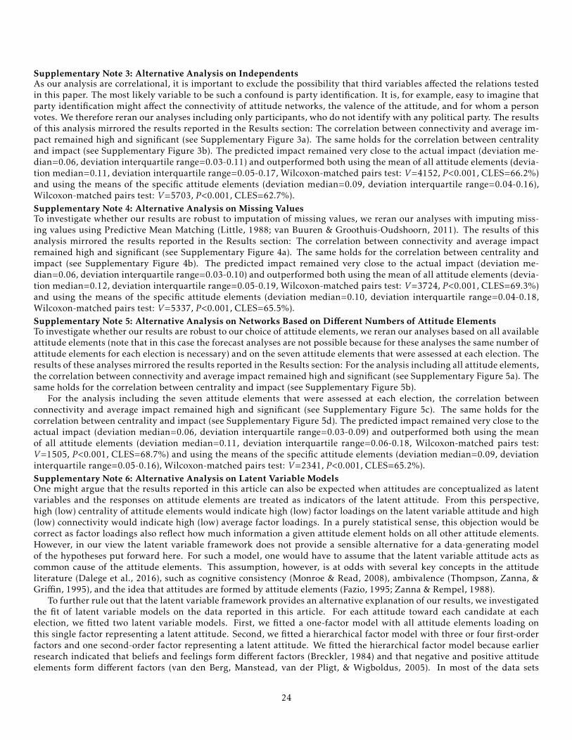
Supplementary Note 3: Alternative Analysis on IndependentsAs our analysis are correlational, it is important to exclude the possibility that third variables affected the relations testedin this paper. The most likely variable to be such a confound is party identification. It is, for example, easy to imagine thatparty identification might affect the connectivity of attitude networks, the valence of the attitude, and for whom a personvotes. We therefore reran our analyses including only participants, who do not identify with any political party. The resultsof this analysis mirrored the results reported in the Results section: The correlation between connectivity and average im-pact remained high and significant (see Supplementary Figure 3a). The same holds for the correlation between centralityand impact (see Supplementary Figure 3b). The predicted impact remained very close to the actual impact (deviation me-dian=0.06, deviation interquartile range=0.03-0.11) and outperformed both using the mean of all attitude elements (devia-tion median=0.11, deviation interquartile range=0.05-0.17, Wilcoxon-matched pairs test: V=4152, P<0.001, CLES=66.2%)and using the means of the specific attitude elements (deviation median=0.09, deviation interquartile range=0.04-0.16),Wilcoxon-matched pairs test: V=5703, P<0.001, CLES=62.7%).Supplementary Note 4: Alternative Analysis on Missing ValuesTo investigate whether our results are robust to imputation of missing values, we reran our analyses with imputing miss-ing values using Predictive Mean Matching (Little, 1988; van Buuren & Groothuis-Oudshoorn, 2011). The results of thisanalysis mirrored the results reported in the Results section: The correlation between connectivity and average impactremained high and significant (see Supplementary Figure 4a). The same holds for the correlation between centrality andimpact (see Supplementary Figure 4b). The predicted impact remained very close to the actual impact (deviation me-dian=0.06, deviation interquartile range=0.03-0.10) and outperformed both using the mean of all attitude elements (devia-tion median=0.12, deviation interquartile range=0.05-0.19, Wilcoxon-matched pairs test: V=3724, P<0.001, CLES=69.3%)and using the means of the specific attitude elements (deviation median=0.10, deviation interquartile range=0.04-0.18,Wilcoxon-matched pairs test: V=5337, P<0.001, CLES=65.5%).Supplementary Note 5: Alternative Analysis on Networks Based on Different Numbers of Attitude ElementsTo investigate whether our results are robust to our choice of attitude elements, we reran our analyses based on all availableattitude elements (note that in this case the forecast analyses are not possible because for these analyses the same number ofattitude elements for each election is necessary) and on the seven attitude elements that were assessed at each election. Theresults of these analyses mirrored the results reported in the Results section: For the analysis including all attitude elements,the correlation between connectivity and average impact remained high and significant (see Supplementary Figure 5a). Thesame holds for the correlation between centrality and impact (see Supplementary Figure 5b).

For the analysis including the seven attitude elements that were assessed at each election, the correlation betweenconnectivity and average impact remained high and significant (see Supplementary Figure 5c). The same holds for thecorrelation between centrality and impact (see Supplementary Figure 5d). The predicted impact remained very close to theactual impact (deviation median=0.06, deviation interquartile range=0.03-0.09) and outperformed both using the meanof all attitude elements (deviation median=0.11, deviation interquartile range=0.06-0.18, Wilcoxon-matched pairs test:V=1505, P<0.001, CLES=68.7%) and using the means of the specific attitude elements (deviation median=0.09, deviationinterquartile range=0.05-0.16), Wilcoxon-matched pairs test: V=2341, P<0.001, CLES=65.2%).Supplementary Note 6: Alternative Analysis on Latent Variable ModelsOne might argue that the results reported in this article can also be expected when attitudes are conceptualized as latentvariables and the responses on attitude elements are treated as indicators of the latent attitude. From this perspective,high (low) centrality of attitude elements would indicate high (low) factor loadings on the latent variable attitude and high(low) connectivity would indicate high (low) average factor loadings. In a purely statistical sense, this objection would becorrect as factor loadings also reflect how much information a given attitude element holds on all other attitude elements.However, in our view the latent variable framework does not provide a sensible alternative for a data-generating modelof the hypotheses put forward here. For such a model, one would have to assume that the latent variable attitude acts ascommon cause of the attitude elements. This assumption, however, is at odds with several key concepts in the attitudeliterature (Dalege et al., 2016), such as cognitive consistency (Monroe & Read, 2008), ambivalence (Thompson, Zanna, &Griffin, 1995), and the idea that attitudes are formed by attitude elements (Fazio, 1995; Zanna & Rempel, 1988).

To further rule out that the latent variable framework provides an alternative explanation of our results, we investigatedthe fit of latent variable models on the data reported in this article. For each attitude toward each candidate at eachelection, we fitted two latent variable models. First, we fitted a one-factor model with all attitude elements loading onthis single factor representing a latent attitude. Second, we fitted a hierarchical factor model with three or four first-orderfactors and one second-order factor representing a latent attitude. We fitted the hierarchical factor model because earlierresearch indicated that beliefs and feelings form different factors (Breckler, 1984) and that negative and positive attitudeelements form different factors (van den Berg, Manstead, van der Pligt, & Wigboldus, 2005). In most of the data sets

24

used here, no negative beliefs were assessed. For these data sets, we fitted a hierarchical factor model with beliefs, negativefeelings, and positive feelings loading on different first-order factors, respectively. For the data sets in which negative beliefswere assessed, we fitted a hierarchical factor model with negative beliefs, positive beliefs, negative feelings, and positivefeelings loading on different first-order factors, respectively. As can be seen in Supplementary Table 3, both the one-factormodels and the hierarchical models fitted poorly. The latent variable framework thus appears to be an unlikely alternativeexplanation of our results.

This discussion on whether our results can also be explained by the latent variable framework is somewhat reminiscentof the discussion regarding the idea that instability of attitudinal responses is indicative of individuals holding nonattitudes(Converse, 1970). Several critiques of this idea pointed out that when measurement error is accounted for, individuals, whoseemingly hold nonattitudes, show stable attitudes (Achen, 1975; Ansolabehere, Rodden, & Snyder, 2008; Judd, Krosnick,& Milburn, 1980). A similar critique might apply to our findings. It is our view, however, that two findings speak againstthis critique. First, if we assume that the intercorrelations of attitude elements are determined only (or foremost) by mea-surement error, then the factor models we fitted should show good fit. This was clearly not the case. Second, systematicvariation of intercorrelations would not be expected from the measurement error perspective. Thus, our finding that con-nectivity of attitudes correlates almost perfectly with the attitude’s impact on behaviour would not be expected from themeasurement error perspective.

25

network structure explains the impact of attitudes on ...(freeman, 1978; opsahl, agneessens, &...

Documents