Network planning by the extended metra potential method(EMPM)Citation for published version (APA):Kerbosch, J. A. G. M., & Schell, H. J. (1975). Network planning by the extended metra potential method(EMPM). (TH Eindhoven. ORS, Vakgr. operationele research : rapport; Vol. KS-1.1). Technische HogeschoolEindhoven.

Document status and date:Published: 01/01/1975

Document Version:Publisher’s PDF, also known as Version of Record (includes final page, issue and volume numbers)

Please check the document version of this publication:

• A submitted manuscript is the version of the article upon submission and before peer-review. There can beimportant differences between the submitted version and the official published version of record. Peopleinterested in the research are advised to contact the author for the final version of the publication, or visit theDOI to the publisher's website.• The final author version and the galley proof are versions of the publication after peer review.• The final published version features the final layout of the paper including the volume, issue and pagenumbers.Link to publication

General rightsCopyright and moral rights for the publications made accessible in the public portal are retained by the authors and/or other copyright ownersand it is a condition of accessing publications that users recognise and abide by the legal requirements associated with these rights.

• Users may download and print one copy of any publication from the public portal for the purpose of private study or research. • You may not further distribute the material or use it for any profit-making activity or commercial gain • You may freely distribute the URL identifying the publication in the public portal.

If the publication is distributed under the terms of Article 25fa of the Dutch Copyright Act, indicated by the “Taverne” license above, pleasefollow below link for the End User Agreement:www.tue.nl/taverne

Take down policyIf you believe that this document breaches copyright please contact us at:openaccess@tue.nlproviding details and we will investigate your claim.

Download date: 23. Feb. 2022

t------·- -.

NETWORK PLANNING BY THE EXTENDED METRA POTENTIAL METHOD

(EMPM)

by Joep A.G.M. Kerbosch and Henk J. Schell

Report KS - 1. 1

june 1975

Translation : Sheila Farrar

John C. Wortmann

Department of Industrial Engineering

Group Operational Research

University of Technology Eindhov~n

The Dutch version of this report is also available; it has

been republished in the 1972 April edition of the journal

INFORMATIE.

Contents

1. Introduction

2. MPM

2.1. History of MPM

2.2. Concise description of MPM

2.2.1. Activity represented by bar

2.2.2. Relation represented by arrow

2.2.3. Negative arrows

2.2.4. Negative cycles

2.3. Transformation of a MPM bar diagram into a directed graph

2.4. Practical objection to MPM

3. Extended MPM

3.1. Extension of allowed relations

3.1.1. The begin-begin relation

3.1.2. the begin-end relation

3.1.3. The end-begin relation

3.1.4. The end-end relation

2

2

2

3

4

7

7

8

8

8

8

9

9

3.1.5. The percentage relation 9

3.1.6. Comparison of relations within Precedence and EMPM 9

3.2. Transformation of an EMPM bar diagram into a directed graph 10

3.2.1. First method: fixed duration of activities

3.2.2. Second method: variable duration of activities

3.2.3. Difference between both methods demonstrated by

means of an example

3.3. EMPM in practice

4. Final conclusion

5. Literature

10

11

12

14

14

15

- I -

1 Introduction

The METRA Potential Method (MPM) , like Precedence, is a network

planning method of the type: "activity on node" [7J. MPM offers

some major advantages compared with other methods of network

planning.

Certain objections can however be made to MPM:

I. The limited practival usefulness.

In the original version of MPM only relations. of the "begin­

begin" type are permitted.

2. The deficiency of a good algorithm (efficient and adequate

error detection) to perform the network computations.

In this paper an extended version of MPM is presented, which we

shall refer to as: "Extended MPM", or EMPM in abbreviated form.

This extension of MPM is fairly simple to implement. It consists

of the following:

All the relations which exist 1n Precendence are possible in EMPM.

The MPM concept of a "negative arrow" and a negative "cycle" are

retained within EMPM. This implies, that a number of relations

are possible in EMPM, which are not allowed in Precedence.

These extra features of EMPM demand a basically different algorithm.

The algorithms published up to now [ 3, 6, 7J all are based on [ 2J •

They are strongly iterative.

A new algorithm is discussed in [4J with the following properties:

- only one iteration is performed when there are no cycles;

- just a few iterations are performed when (negative) cycles are

present.

2 MPM

2.1 History of MPM

The MPM method was developed in France in 1958 by the advisory

bureau SEMA [ 6J. The method was used for the first time at the

construction of nuclear power plants on the Loire.

- 2 -

"Metra" originates from a group of advisory bureau x (including SEMA)

of the same name which offers its clients MPM as a planning method.

The method is called: "potential method" because of the analogy which

exists - from a mathematical point of view - with the system of

potentials in an electrical network.

2.2 Concise description of MPM

MPM is a network planning method of the type "activity on node" as

stated in the introduction.

However we prefer to speak of "activity on bar", as the activities

in the bar diagram are not represented by nodes but by bars.

2.2.1

2.2.2

Activity represented by bar

The project consists of activities, which are represented ~n MPM

by bars.

An example:

activity I

Re~ation represented by arrow

We shall first state some difinitions ~n order to simplify the further

description:

- I and J are both activities;

- B(I) is the moment at which activity I starts;

- L(I,J) is the duration of the relation between I and J.

In other words the length of the arrow between I and J.

In MPM only relations, which refer to the moments at which activities

start, are permitted. In the terminology defined above this will mean,

that we only can represent relations between B(I) and B(J).

2.2.3

- :3 -

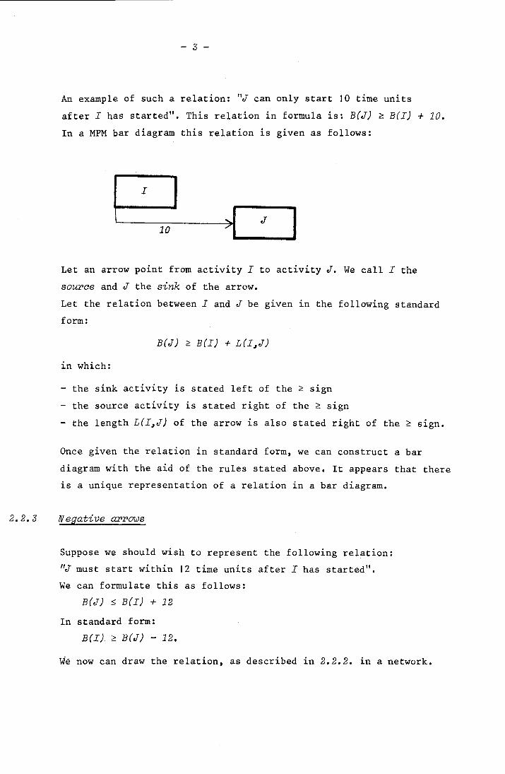
An example of such a relation: "J can only start 10 time units

after I has started". This relation in formula is: B(J} ~ B(I) + 10.

In a MPM bar diagram this relation is given as follows:

I

..... J10 /

Let an arrow point from activity I to activity J. We call I the

source and J the sink of the arrow.

Let the relation between I and J be given ~n the following standard

form:

B(J) ~ B(I} + L(I~J}

~n which:

- the sink activity ~s stated left of the ~ s~gn

- the source activity is stated right of the ~ sign

- the length L(I~J) of the arrow is also stated right of the ~ s~gn.

Once given the relation ~n standard form, we can construct a bar

diagram with the aid of the rules stated above. It appears that there

is a unique representation of a relation in a bar diagram.

Negative appows

Suppose we should wish to represent the following relation:

"J must start within 12 time units after I has started".

We can formulate this as follows:

B(J) $ B(I) + 12

In standard form:

B(I) ~ B(J} - 12.

We now can draw the relation, as described ~n 2.2.2. ~n a network.

2.2.4

- 4 -

-4 I I.----12----.1I_J_1

From the above it appears that in this concept the length L(I~J)

of an arrow may be negative.

In permitting this kind of relations MPM really is distinct from

all other known network methods offering the user the possibility of

formulating a more realistic model of a project.

In practice one ~s often faced with relations of the following kind:

"A must start within so many days after B"~ "e must start before a

certain date etc.". This kind of relations cann't be used in the

model (= bar diagram) when dealing with other network planning

methods.

It is out of the question that such omissions ~n the model may lead

to incorrect results and decisions.

Negative cycZes

In MPM also combinations are permitted of the relations, described in

2.2.2. and 2.2.3. For instance: "J must start between the 10th and

the 12th time unit after I has starte

In formula:

and

B(J) ~ B(I) + 10

B(J) ::; B{I) + 12in standard form:

B(I) ~ B(J) - 12.We then find the bar diagram:

r--- rto

-12 J

- 5 -

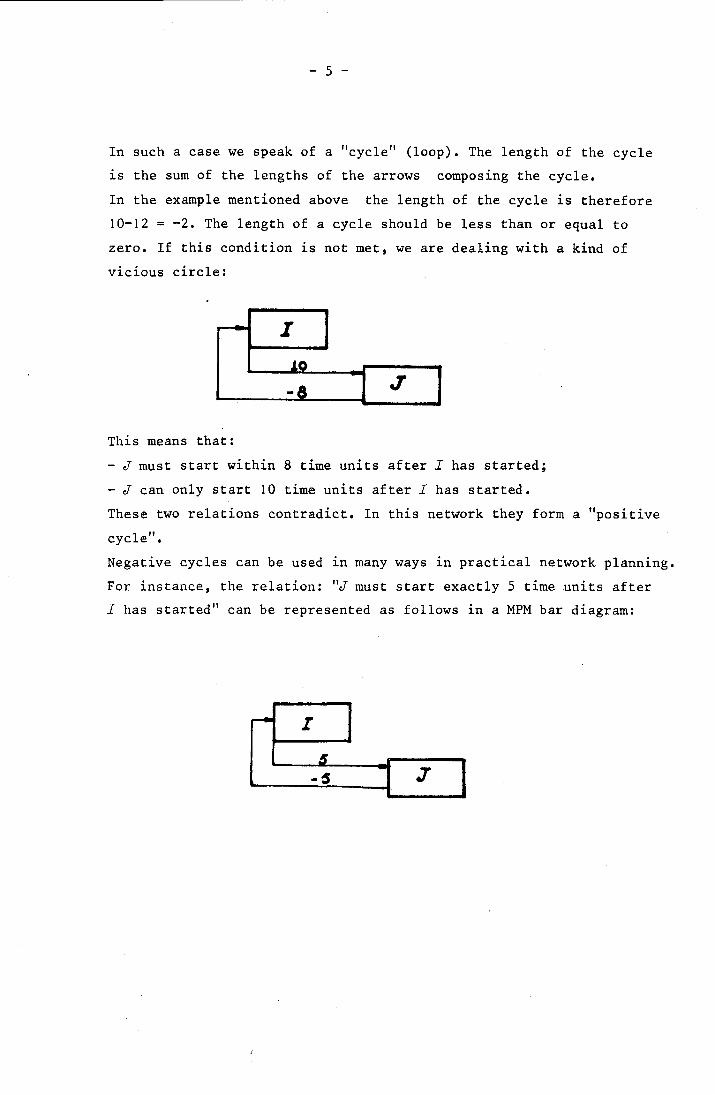
In such a case we speak of a "cycle" (loop). The length of the cycle

~s the sum of the lengths of the arrows composing the cycle.

In the example mentioned above the length of the cycle is therefore

10-12 = -2. The length of a cycle should be less than or equal to

zero. If this condition is not met, we are dealing with a kind of

vicious circle:

r---- I

.10

-8 J

This means that:

- J must start within 8 time units after I has started;

J can only start 10 time units after I has started.

These two relations contradict. In this network they form a "positive

cycle".

Negative cycles can be used ~n many ways ~n practical network planning.

For instance, the relation: "J must start exactly 5 time units after

I has started" can be represented as follows in a MPM bar diagram:

~ r~

-~j

- 6 -

In a network far more complicated cycles may be found.

For example:

-116 K

I

s J

or : 3 J

I~

~ - k2

-15~ L

In practice the cycles often are fairly simple.

It is however essential, that the algorithm and the computational

program correctly can handle the most complicated cycles and this

makes the problem mathematically interesting.

- 7 -

2.3 Transformation of a MPM bar diagram into a directed graph

After a project has been split up into activities and the relations

between these activities have been established, computations must be

performed on the produced bar diagram. In other words, planning data

such as: "earliest start", "latest start", etc. have to be determined.

The bar diagram must be transformed into a directed graph (network),

before these computations can start. Note, that this also holds for

Precedence. This transformation may be part of the program and is

necessary due to the fact, that there exists no "bar diagram theory";

we however can use graph theory. This graph theory provides us with

concepts, theorems and algorithms. The transformation is very simple

in the MPM case, because only relations are permitted between the

start moments of activities. The start moments are considered to be the

nodes of the graph, and the relations the arrows.

2.4 Practical objection to MPM

As a method of planning MPM is difficult to handle. The reason for this

is that only relations between start moments are permitted. For example

suppose we wish to represent the relation: "activity J may only start

when activity I has finished". This can be depicted as follows:

I

p J'

Here the duration of activity I determines the length of the arrow.

For the one who produces the bar diagram this involves a lot of extra

work. In addition, if the duration of I is changed, the length of the

arrow must be adjusted accordingly. The chance of making mistakes becomes

considerably greater.

- 8 .,.

If we wish to represent the same relation in Precendence, we find:

D,-1___._J IThis representation ~s much more logical and straightforward.

3 Extended MPM

3.1 Extension of the permitted relations

The objection to MPM mentioned above is removed in a quite simple

way in EMPM. In EMPM the following relations are permitted:

3.1.1 The begin-begin relation

This is in the form of:

"activity J only may start p time units after activity I has started".

In diagram:

oI

L p --1_J__1

3.1.2 The begin-end relation

"Activity J only may finish p time units after activity I has

started". In diagram:

I J

p

- 9 -

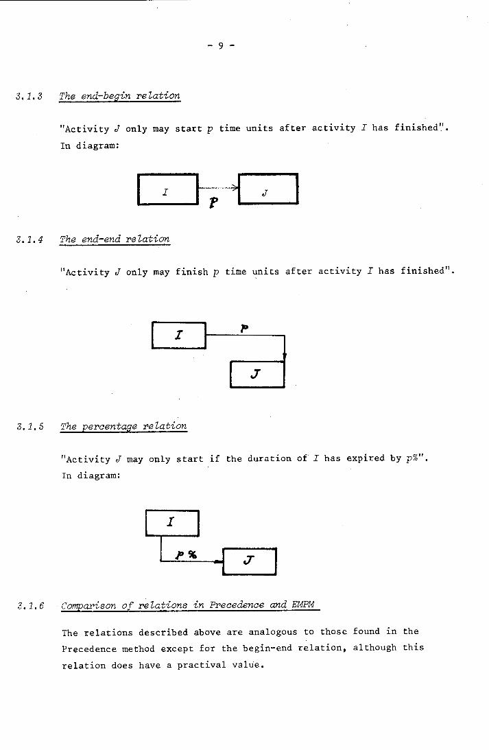
3.1.3 The end-begin relation

"Activity J only may start p time units after activity I has finished".

In diagram:

I I ~ II JP

3.1.4 The end-end relation

"Activity J only may finish p time units after activity I has finished".

I 'fO

J

3.1.5

3.1. e

The percentage relation

"Activity J may only start if the duration of I has expired by p%".

In diagram:

I

}O~ J

COmparison of relations in Precedence and EMPM

The relations described above are analogous to those found in the

Precedence method except for the begin-end relation, although this

relation does have a practival value.

- 10 -

For example, the relation: "Activity J must start between the 2nd and

the 4th time unit after activity I has finished" can be represented

in EMPM as follows:

f_I L2

The arrow from J to I, which is -4 in length, is a begin-end relation.

3.2 Transformation of an EMPM bar diagram into a directed graph

The transformation is more complicated in the case of an EMPM bar

diagram. There are two possibilities, which we shall discuss now.

3.2.1 Fixed duration of activities

The first possibility assumes the estimated duration of an activity

being a hard fact. We shall show that the transformation of an EMPM

bar diagram into a directed graph roughly occurs in the same way as

1n the case of a MPM bar diagram. For this purpose, we define:

I and J are two activities;

D(I} is the duration of I;

B(I} 1S the start moment of I;

E(I} 1S the finish moment of I.

The duration of the activity 1sconsidered to be fixed; therefore, the

following applies:

E(I) =B(I) + D(I) and E(J) =B(J) + D(J).

With the aid of these two relationships, we can transform the EMPM

relations of 3.1.2 through J.l.5 in a simple way into relations of

the begin-begin type (3.1.1). For example, we take an end-end relation.

In formula: E(J) ~ E(I) + P

or B(J) + D(J) ~ B(I) + D(I) + p~ in standard form:

B(J) ~ B(I) + D(I) - D(J) + p

We now have created a begin-begin relation, with a duration of:

D(I) - D(J) + p.

By transforming all the relations in a EMPM bar diagram into begin­

begin relations, we have in fact constructed a MPM network. We already

showed in 2.3 how we can interpret this as a directed graph.

3.2.2

- 11 -

Second method: variabZe activity duration

In this method, we assume a certain amount of variability ~n the

duration of an activity. This is only of value if:

the activity can be interrupted

the activity can be temporized, e.g. by using less resources.

The "normal" duration of an activity is taken to be the lower bound

of the duration. This means the number of time units required for

the execution of the activity, using "normal" capacity, "normal"

pace of work, etc. In other words, the activity duration according

to the first method (3.2.1).

The upper bound of the activity duration is the number of time

units related to the use of minimum capacity or interruption.

Example:

Activity A can be completed by 5 men in 3 days, or by 1 man in 18

days. Intermediate possibilities also are permitted. The lower bound

of the activity duration then would be 3, and the upperbound 18.

Therefore: 3 ~ D(A) ~ 18.

A bar diagram of such a type can be transformed as follows into a

directed graph:

the begin and end points of the activities are represented by

nodes;

arrows represent the relations supplemented with one pair of

arrows per activity, which connect the begin and end point of

the activity.

Activity A can be represented as follows:

---

B(A)

-18

P E(A)

- 12 -

Note, that if the lowerbound equals the upperbound, we are dealing

with an activity of fixed duration, e.g. an activity which lasts exactly

5 time units.

B( •

5

-5

E(. )

The method described under 3.2.1 may be considered as a special case

of the method mentioned here; however, the percentage relation is not

allowed when using a variable activity duration.

Note, that it is no longer necessary to transform the relations into

begin-begin relations.

Difference between both methods demonstrated by means of an example

In order to make the difference between the two methods evident, we shall

give an example.

A project consists of the following three activities:

I (electricians' work) which takes 5 days;

J (plasterers' work) which takes 3 days;

K (painters' work) which takes 4 days.

The three activities can be carried out simultaneously, on condition that:

the eclectricians begin at least one day before the plasterers begin;

the plasterers do not complete the work before the electricians have

finished.

These same restrictions also apply to the painters' work in relation to

the plasterers' work. We can denote the relations in formula as follows:

B(J) ~ B(I) + 1~ E(J) ~ E(I)~ B(K) ~ B(J) + 1~ E(K) ~ E(J).

In diagram:

I0

1 J' 0

~ /(

- 13 -

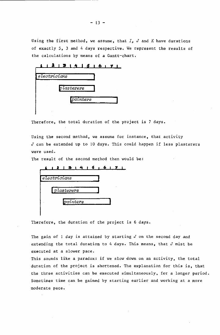
Using the first method, we assume, that I~ J and K have durations

of exactly 5, 3 and 4 days respective. We represent the results of

the calculations by means of a Gantt-chart.

eLectricians

WLasterers 1

Ipainters I,'"---------'

Therefore, the total duration of the project LS 7 days.

Using the second method, we assume for instance, that activity

J can be extended up to 10 days. This could happen if less plasterers

were used.

The result of the second method then would be:

e ectncnans

l"",e..L_a_s_t_e;.;r;.;e;.;r;.;s~ J

leainters ],.....- ---------

Therefore, the duration of the project LS 6 days.

The gain of 1 day is attained by starting J on the second day and

extending the total duration to 4 days. This means, that J must be

executed at a slower pace.

This sounds like a paradox: if we slow down on an activity, the total

duration of the project is shortened. The explanation for this is, that

the three activities can be executed simultaneously, for a longer period.

Sometimes time can be gained by starting earlier and working at a more

moderate pace.

- 14 -

3.3 EMPM in praotioe

A computer program has been developed dealing with EMPM networks,

which is called ANNETTE (Activity in Node Networkanalysis University

of Technology Eindhoven) [5J. The term "dealing with" should be taken

~n the broadest sense of the word; this comprises not only the trans­

formation into a graph and the performing of network computations,

but also all the administrative computations like file handling, report

printing, etc. This makes the program not only suitable for the initial

planning, but also for continuous project control. We are adopting the

method, described under 3.2.2 for the transformation of a bar diagram

into a graph. In the building industry we are using and testing EMPM

on certain projects concerning planning and project control. Recently

EMPM was adopted at an oil refinery maintainance project. The results

reached So far are very satisfactory.

4 Final Conolusion

EMPM is a network planning method combining the advantages of MPM and

Precedence. The advantages for the EMPM user are:

the variety of relations, which makes Precedence easy to deal with;

the possibility of constructing a more realistic model by using ne­

gative arrows and cycles.

- 15 -

5 Literature

[I] Dibon, M. L. ,

Ordonnancement et potentiels, Methode MPM,

Herman, Paris (1970)

[2J Ford, L.R. and D.R. Fulkerson,

Flows in Networks,

Princeton, New Yersey (1962)

[3J Gewald, K and D. Sauler,

Ein ALGOL-Prograrnrn fur die METRA-potential Methode,

Ablauf, Planung und Forschung 7(1966) Heft 4, p. 199.

[4J Kerbosch, Joep A.G.M., Henk J. Schell and John C. Wortmann,

An algorithm for network planning by the metra-potential method,

Technical report KS-2.1.,

University of Technology Eindhoven (1975).

[5J Kerbosch, Joep A.G.M. and Henk J. Schell,

User Manual ANNETTE 3,

Technical report KS-3.1.,

University of Technology Eindhoven (1975)

[6J Roy, B.

Graphes et ordonnancements,

Revue Fran~aise de recherche operationelle.

nr. 25, 6 (1962.10), page 323.

[n Wille, H. K. Gewald und H.D. Weber,

Netzplantechnik, Methoden zur Planung und Ueberwachung von

Projekten,

Band I. Zeitplantechnik, Oldenbourgh, Munchen (1966).