Network Link Dimensioning based on StatisticalAnalysis and Modeling of Real Internet Traffic

Mohammed AlasmarSchool of Engineering and Informatics

University of SussexBrighton, UK

m.alasmar@sussex.ac.uk

Nickolay ZakhleniukComputer Science and Electronic Engineering

University of EssexColchester, UKnaz@essex.ac.uk

Abstract—Link dimensioning is used by ISPs to properlyprovision the capacity of their network links. Operators haveto make provisions for sudden traffic bursts and networkfailures to assure uninterrupted operations. In practice, trafficaverages are used to roughly estimate required capacity. Moreaccurate solutions often require traffic statistics easily obtainedfrom packet captures, e.g. variance. Our investigations on realInternet traffic have emphasized that the traffic shows highvariations at small aggregation times, which indicates that thetraffic is self-similar and has a heavy-tailed characteristics.Self-similarity and heavy-tailedness are of great importance fornetwork capacity planning purposes. Traffic modeling processshould consider all Internet traffic characteristics. Thereby, thequality of service (QoS) of the network would not affected byany mismatching between the real traffic properties and thereference statistical model. This paper proposes a new class oftraffic profiles that is better suited for metering bursty Internettraffic streams. We employ bandwidth provisioning to determinethe lowest required bandwidth capacity level for a network link,such that for a given traffic load, a desired performance target ismet. We validate our approach using packet captures from realIP-based networks. The proposed link dimensioning approachstarts by measuring the statistical parameters of the availabletraces, and then the degree of fluctuations in the traffic hasbeen measured. This is followed by choosing a proper model tofit the traffic such as lognormal and generalized extreme valuedistributions. Finally, the optimal capacity for the link can beestimated by deploying the bandwidth provisioning approach.It has been shown that the heavy tailed distributions give moreprecise values for the link capacity than the Gaussian model.

Index Terms—Network link dimensioning, Bandwidth pro-visioning, Traffic Modeling, Quality of Service, Self-similarity,Heavy tail

I. INTRODUCTION

Recently, there is an increasing demand on high perfor-mance services in the Internet; these services include data,voice, and video transmission, these three main services aretermed as triple-play services. In the context of IP networks,the validation of the network depends on the examinationof the QoS metrics such as delay, delay-jitter, packet loss,availability and throughput [1]. These metrics are describedin a committed contract between the users and the serviceproviders which is known as service level agreement (SLA).The above mentioned QoS metrics are mainly relied onbandwidth planning of the network. This indicates theimportance of sufficient bandwidth to be provisioned.

A commonly used bandwidth allocation mechanisms inthe IP networks are defined in RFC 1633 and RFC 2475, thetwo IETF models refer to the integrated services (Intserv)and the differentiated services (Diffserv) respectively [2], [3].The complexity of DiffServ and IntServ in deploying theQoS metrics can be avoided by using simple bandwidthprovisioning mechanism. The main idea behind bandwidthprovisioning is to allocate sufficient bandwidth to the linkuntil achieving satisfied performance, which ensures thatthe SLA requirements are met [4].

In the conventional methods of assurance the link band-width, we just apply rules of thumb, such as bandwidthover-provisioning by upgrading the link bandwidth to 30%of the average traffic value [4]. This ensures there is notraffic congestion will take place in the link. The drawbackof this mechanism is that it can provide by more bandwidththan is actually needed, intuitively, this will increase thecost of connection. On the other hand, the bandwidthprovisioning approach provides the link by the essentialbandwidth that guarantees the required performance [5].

The timescale of traffic aggregation is critical in evaluat-ing the link capacity. Fig. 1 shows the throughput (bits/sec)of a captured trance over an interval of 900 sec at differenttimescales: 1 sec, 30 sec and 300 sec. It is obvious thatmore fluctuations (burstiness) appear at small values ofaggregation time. The more the fluctuations, the more thethroughput values are far from the mean, which indicatesmore variation. Therefore, the conventional techniques ofbandwidth allocation are imprecise at small timescales, andthis will break the SLA requirements.

Figure 1: The throughput of a captured traffic at differenttimescales

arX

iv:1

710.

0042

0v1

[cs

.NI]

1 O

ct 2

017

There is a large body of work aiming to study the Internettraffic properties. Some studies [6]–[9] show that the Inter-net traffic has the following properties: self-similarity, trafficburstiness and heavy tails. Consequently, the designing ofan optimal Internet traffic model should consider theseproperties. This model plays a critical role in planningnetworks.

Meent et al. [4] introduced a new bandwidth provision-ing formula, which relies on the statistical parameters ofthe captured traffic and a performance parameter. Theydemonstrated that the Internet traffic is bursty over a widerange of aggregation times. They assumed that the Internettraffic can be characterised by a Gaussian distribution.Their assumption about the applicability of a Gaussiandistribution to represent the Internet traffic is based onsome related works as [10], [11]. However, this work hasmissed two major investigations, which are the validation ofGaussianity assumption and the testing of the self-similarityof the Internet traffic.

In some situations, we cannot observe complete infor-mation about the traffic. Employing the efficient estimationmethod and then choosing the best model in this situationare very important. In [12], it is concluded that the tailsof the traffic do not track Gaussian distribution, and it issuggested that heavy-tailed distributions are more accuratein representing the Internet traffic. These distributions havehigher peaks and heavier tails than normal distributions.Besides, they have good statistical and reliability proper-ties. Examples of heavy-tailed distributions are Log-normaldistribution, Pareto distribution, Weibull distribution, Gen-eralized Extreme Value (GEV) distribution and log-gammadistribution. These distributions are more accurate in rep-resenting long-range dependence and self-similar traffic. Inthis context, the following studies [13]–[16] have reviewedevidence that Internet traffic is characterised by long-taileddistributions.

In this paper we present a statistical analysis and bestfitted distribution model of IP-based Internet traffic. Wedemonstrate that the Internet traffic is not perfectly fittedwith the normal distribution. The fact that Gaussian distri-bution characterises several aggregated traffics is based onthe central limit theorem [17]. However, this theory is validfor independent and identically distributed (iid) randomprocesses and it fails if there are dependences between anycombinations in the distribution. Therefore, the resultantempirical performance criterion of bandwidth provisioningapproach over Gaussian model does not achieve the targetperformance, as more attention has to be paid to the tailvalues. As a result of the fitting tests and the validation ofthe empirical performance, we found that the lognormaland the GEV models are the proper heavy tails distributionfor the network traffic.

This paper makes the following specific contributions.

• Investigation self-similarity property in Internet traffic(see section II), the presence of this property means

that the traffic is burstiness which indicates moreextreme values present at small aggregation times.

• Finding an optimal statistical model to characterisethe Internet traffic(see section IV), this model has toconsider the network traffic’s properties. Whilst thetraditional network traffic follows a Markovian model,this model is not valid in expressing the Internet traffic.This failure comes from the fact that the Internet trafficis bursty on a wide range of time scales [18].

• Deploying bandwidth provisioning approach over thesuggested models (see sections V and VI).

In our experiments, we used 653 of real network traffictraces that have been captured at five locations , whichdiffer substantially, in terms of both size and the typesof users [19]. The traces were captured over a period of15 minutes during different times in the day and thenight. Table I summarises the details of the five monitoredlocations at a university campus.

Table I: The details of the monitored locations

Location Description#Packet

traces

1. Residential

network

300 Mbps Ethernet link connects

2000 students

(each has 100 Mbps access link)

15

2. Research

institute

network

1 Gbps Ethernet link connects

200 researchers

(each has 100 Mbps access link)

185

3. Large

college

1 Gbps Ethernet link connects

1000 employees

(each has 100 Mbps access link)

302

4. ADSL

access

network

1 Gbps ADSL link is used by

hundreds of users (each has from

256 kbps to 8 Mbps access link)

147

5. Educational

organisation

100 Mbps Ethernet link connects

135 students and employees

(each has 100 Mbps LAN)

4

II. SELF-SIMILARITY IN INTERNET TRAFFIC

The Internet networks traffic (packet-based networks)performs self-similarity; this is due to the existence ofburstiness over a wide range of timescales. In conventionalmodels, the distribution of the packets length of the Inter-net traffic becomes smoother instead of becoming burstyduring the aggregation process. Therefore, the conventionalmodels do not have the ability to represent the Internetnetworks traffic. Because of the importance of self-similarityphenomenon on modeling real Internet traffic, this sectionpresents the results of the self-similarity tests on the cap-tured traces. Firstly, we discuss the properties of self-similartraffics, which have been concluded at several studies thatare established practically to measure and analysis thestatistical characteristics of self-similar traffic of a packet-based networks [6], [7], [20], [21].

A. The correlation function is Long-range dependence (LRD)

This property measures the robust dependence betweenthe present values and the old values of any randomprocess. In order for any process to be LRD, the auto-correlation function has to decrease hyperbolically, thiscan be satisfied by getting non-summable autocorrelation

function:∞∑

k=−∞r (k) = ∞. In contrast, the autocorrelation

function of a short-range dependence processes decreaseexponentially [22]. Hence, for any process that is self-similar, its autocorrelation function can be formulated asfollows:

r (k) ∼ ak−β,k →∞ (1)

where 0 < β < 1, which is a positive constant value anda is a scaling factor. This means that the central limittheorem is not applicable on a self-similar traffic, as it isjust applicable on iid processes.

B. Slowly decaying variance

The aggregation process X (m)k can be defined as follows:

X (m)k = 1

m

km∑i=km−m+1

Xi = 1

m(Xkm−m+1 + ...+Xkm) (2)

where X (m)k is the averaging value of time series of each

non-overlapping neighbouring blocks each of size m, whilek is the index of each block and N is the total size of thetime series. The variance of the aggregated process X m ofa self-similar process can be described as follows [23]:

V ar (X (m)k ) = 1

N /m

N /m∑k=1

(X (m)k −X m) ∼ m−β (3)

for all m = 1,2,3, ... , k = 1,2, ..., N /m and 0 <β< 1 where X m

is the mean value of the segment X (m), which is calculatedas follows:

X m = 1

N /m

N /m∑k=1

X (m)k

C. The power spectrum has a power-law distribution aroundzero frequency

For any discrete sequence Xn of length N, the powerspectrum S(ω) can be calculated by using the discreteFourier transform (DFT) or the fast Fourier transform (FFT)as follows [23]:

S(ω) = 1

2πN

∣∣∣∣∣ N∑n=1

Xne j nω

∣∣∣∣∣2

(4)

where ω= 2πn/N and −π≤ω≤πThe power spectrum of a self-similar process follows a

power law and it is centred at the origin. This can bedescribed as follows:

S(ω) ∼ |ω|−δ as ω→ 0, 0 < δ< 1 (5)

III. THE STATISTICAL TESTS OF SELF-SIMILARITY

There are several statistical tests to examine the self-similarity of any distribution or process. We are going touse three of these tests: R/S test, time-variance plot, andPeriodogram method. The estimated value of the Hurstparameter in each test gives evidence about the presenceof the self-similarity in the examined trace. If 0.5 < H < 1this implies that the traffic is self-similar [23].

A. Variance-Time Test

The logarithm of the two sides in equation (3) gives:

log[

var (X (m)k )

]∼−βlog (m), as m →∞ (6)

The value of β is obtained from the log-log plot:

log[

var (X (m)k )

]versus l og (m) where β is the slope of the

fitted line (using least-squares method) in this plot. Forslowly decaying variance the slope of the fitted line β hasto be between -1 and 0. Where the Hurst parameter isequal to H = 1−β/2.

B. Rescaled-Range (R/S) Test

R/S test [24] demonstrates to measure the variability inthe traffic. For a series X (t ) = X1, X2, ..., XN of N samples andsample mean µn . The range R is the difference betweenthe maximum and minimum values of the cumulativesummation of the deviation values at each sample point,as follows:

R(n) = max1<t<n

t∑i=1

(Xi −µn)− mi n1<t<n

t∑i=1

(Xi −µn) (7)

The relation between Hurst parameter and R/S value canbe described as follows:

E

[R(n)

S(n)

]∼ cnH ,as n →∞

where S(n) is the standard deviation of the samples and c isa positive constant number. The logarithm of the two sidesgives:

log

(E

[R(n)

S(n)

])∼ Hl og (n)+ log (c) (8)

Thus, the Hurst parameter is equal to the slope of thefitting line on the log-log graph: log

(E

[R(n)S(n)

])versus

log (n).

C. Periodogram Test

This method is characterised as a frequency domainestimation of the Hurst parameter, and it is more precisethan the previous tests. The advantage of this methodover the previous tests comes from the fact that there isno need for aggregation or combination of the originaltraffic points during the calculation of the power spectrum.The power spectrum density S(ω) can be calculated fromequation (4). It is important to note that the existence of

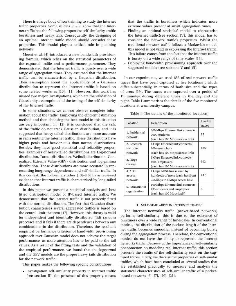
self-similarity will affect the power spectrum at the bandof the low frequencies i.e. as ω→ 0. This indicates that thepower spectrum of self-similar process follows a power lawdistribution as ω→ 0, as shown in Fig. 2.

Figure 2: The power spectrum density of an Internet traffic

From equation (5) S(ω) can be obtained as follows:

S(ω) ∼ |ω|1−2H , as ω→ 0 (9)

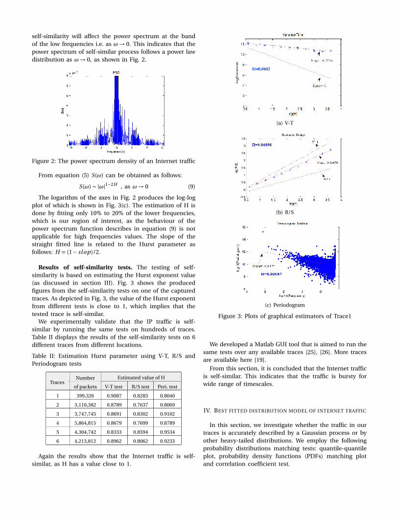
The logarithm of the axes in Fig. 2 produces the log-logplot of which is shown in Fig. 3(c). The estimation of H isdone by fitting only 10% to 20% of the lower frequencies,which is our region of interest, as the behaviour of thepower spectrum function describes in equation (9) is notapplicable for high frequencies values. The slope of thestraight fitted line is related to the Hurst parameter asfollows: H = (1− sl op)/2.

Results of self-similarity tests. The testing of self-similarity is based on estimating the Hurst exponent value(as discussed in section III). Fig. 3 shows the producedfigures from the self-similarity tests on one of the capturedtraces. As depicted in Fig. 3, the value of the Hurst exponentfrom different tests is close to 1, which implies that thetested trace is self-similar.

We experimentally validate that the IP traffic is self-similar by running the same tests on hundreds of traces.Table II displays the results of the self-similarity tests on 6different traces from different locations.

Table II: Estimation Hurst parameter using V-T, R/S andPeriodogram tests

Estimated value of HTraces

Number

of packets V-T test R/S test Peri. test

1 399,326 0.9087 0.8283 0.8040

2 3,110,382 0.8789 0.7637 0.8069

3 3,747,745 0.8691 0.8302 0.9102

4 5,864,815 0.8679 0.7699 0.8789

5 4,304,742 0.8333 0.8594 0.9534

6 4,213,812 0.8962 0.8062 0.9233

Again the results show that the Internet traffic is self-similar, as H has a value close to 1.

(a) V-T

(b) R/S

(c) Periodogram

Figure 3: Plots of graphical estimators of Trace1

We developed a Matlab GUI tool that is aimed to run thesame tests over any available traces [25], [26]. More tracesare available here [19].

From this section, it is concluded that the Internet trafficis self-similar. This indicates that the traffic is bursty forwide range of timescales.

IV. BEST FITTED DISTRIBUTION MODEL OF INTERNET TRAFFIC

In this section, we investigate whether the traffic in ourtraces is accurately described by a Gaussian process or byother heavy-tailed distributions. We employ the followingprobability distributions matching tests: quantile-quantileplot, probability density functions (PDFs) matching plotand correlation coefficient test.

A. The quantile-quantile plot (Q-Q plot)

Q-Q plot is a powerful visualization test which can assessthe degree of similarity between different distributions. Themain idea of the Q-Q plot is to compare the observed datawith one of the well-known distributions such as normaldistribution. The quintiles are defined as the values thatare taken from the random variables every regular interval.The x-axis of the Q-Q plot represents the quantiles of thereference distribution while y-axis represents the quantilesof the observed samples [27]. Q-Q plots are created byplotting the pair(

F−1(

i

n +1

),S(i )

), i = 1, ...,n (10)

where n is the number of samples, F−1 is the inverse cu-mulative distribution function of the reference distributionand S(i ) is the observed samples. The two distributions arematched if the scattered points of the two quantiles followa straight fitting line.

B. The linear correlation coefficient test

The covariance measures the strength of the relationbetween two random variables. For strong measuring ofgoodness-of-fit, the normalized version of the covariance,which is known as linear correlation coefficient can beused. The normalization factor is the multiplication of thestandard deviation of both: the empirical distribution stan-dard deviation σS(i ) and the reference distribution standarddeviation σxi . Hence, the correlation coefficient can bewritten as [27]:

γ= cov(S(i ), xi )

σS(i )σxi

=∑n

i=1

(S(i ) − µ̂

)(xi − x̄)√∑n

i=1

(S(i ) − µ̂

)2 .∑n

i=1 (xi − x̄)2(11)

where S(i ) is the observed samples, and its mean value:µ̂= 1

n

∑ni=1 S(i ), while xi is the reference distribution samples

which can be calculated from the inverse CDF of thereference random variable: xi = F−1

( in+1

)and its mean

value: x̄ = 1n

∑ni=1 xi .

The value of the correlation coefficient can vary between:−1 ≤ γ≤ 1. Note that as the value of γ changes from ±1 to0, then relation strength will drop from strong to moderateand finally to weak strength around the zero value. For thepurpose of getting stronger goodness-of-fit, the acceptablevalue of γ is suggested to be above 0.95.

Results of testing the matching between the Internettraffic and the suggested models

Fig. 4 shows the results of applying Q-Q plot test onTrace1 at different aggregation times (T=0.01 sec and T=1sec) and by using different reference distributions (Normal,Lognormal and GEV). Besides, it shows the PDF of both thecaptured traffic (the blue bars in the sub-figures) and thefitting curve of the reference distributions (the red curvesin the sub-figures). The aggregation times are chosen to be

reasonably small to include traffic fluctuations as discussedin the introduction.

(a)

(b)

(c)

Figure 4: Q-Q plot, value and PDF at different timescalesfor (a) Normal (b) Lognormal (c) GEV distributions

From Fig. 4(a), it is noticeable that the captured trafficis not perfectly fitted with the normal distribution. Themismatching between the two distributions takes placeat the tails values, as the Q-Q points are deviated fromthe straight lines at the tails. In addition, the correlationcoefficient values do not indicate strong correlation be-tween the distributions, as the values of γ are below 0.95.

Based on the analysis of these results, it is obvious thatwe need to pay more attention to the tails. On the otherhand, Fig. 4(b)-(c) show that the captured traffic is perfectlyfitted with the GEV distribution and it is almost fittedto the lognormal distribution. In addition, the correlationcoefficient values indicate strong correlation between thedistributions, since the values of γ are larger than 0.95.Unlike normal distribution, the tails in the Q-Q plots showsome extreme values which could not be represented bythe reference lines.

It is concluded that heavy-tailed distributions such aslognormal and GEV distributions are more accurate inrepresenting the Internet traffic. This conclusion is based ontesting hundreds of traces from different locations by usingour developed tool [25]. The obtained results are alwaysclose to the results shown in Fig. 4.

V. BANDWIDTH PROVISIONING APPROACH

In this section we deploy the bandwidth provisioningmechanisms based on the statistic distributions that havebeen proved to be more accurate in characterising theInternet traffic. The goal of the bandwidth provisioningapproach is to enhance the channel capacity without extrabandwidth. Although the normal model is not suitable torepresent the network traffic as explained in the previoussection, we will continue under the gaussianity assumptionto demonstrate that this model gives unsatisfactory resultsin deploying the bandwidth provisioning approach.

In the bandwidth provisioning approaches, linktransparency is selected as QoS criteria. The followinginequality is used for the purpose of accurate checking ofthe link transparency [27]:

P (A(T ) ≥C T ) ≤ ε (12)

It is obvious from this inequality that the probabilityof finding the captured traffic over a specific period oftimescale A(T )/T larger than the link capacity has to besmaller than the value of the performance criterion ε. Thevalue of ε represents the probability of packet loss and itsvalue has to be chosen carefully by the network providerin order to meet the specified SLA; in general, ε has tobe below the probability 10−2. Likewise, the value of theaggregation time T should be sufficiently small so that thefluctuations in the traffic can be modeled as well.

Mainly, optimising the link capacity will be investigatedbased on the following five bandwidth provisioning (BWP)approaches:- Approach 1: BWP through direct calculations under thestandard normal PDF- Approach 2: BWP using extended formula of the Gaussianmodel- Approach 3: BWP using Meent’s approximation formula- Approach 4: BWP based on lognormal distribution model- Approach 5: BWP based on GEV distribution model

A. Approach 1: BWP through direct calculations under thestandard normal PDF

Under the Gaussianity behaviour, the captured trafficA(T ) is described as follows,

A(T ) ∼ Nor m(µT,υ(T )) (13)

where µA = µT is the mean value (in bits) and υ(T ) isthe variance (in bits2) of A(T ).

The link transparency condition (equation 12) can besolved by finding the value of C which satisfies the valueof the performance criterion ε, as shown in Fig. 5. Formore simplicity, the variable A(T ) has to be standardizedby mapping it from normal distribution A(T ) to standardnormal distribution Z . This will make the probabilitiescalculations simpler. This transformation is given by:

A(T ) =µT +√υ(T )Z (14)

Figure 5: The normal and the standard normal distributionof A(T)

By substituting for A(T ) from equation (14) into equation(12) we obtain:

P(µT +

√υ(T )Z ≥C T

)≤ ε

Then,

P

(Z ≥ C T −µTp

υ(T )

)≤ ε

Now,

T

(C T −µTp

υ(T )

)= 1−Φ

(C T −µTp

υ(T )

)≤ ε (15)

where T (z) is the complementary cumulative distributionfunction (CCDF) of the standard normal distribution, andΦ(z) is the cumulative function, where T (z) = 1−Φ(z) andΦ(z) = P (Z ≤ z).

Hence, from equation (15) the value of the link capacitycan be written as follows:

C1: C =Φ−1 (1−ε)

√υ(T )

T 2 +µ (16)

where C is the link capacity (in bits per second), υ(T )is the variance of the captured traffic (in bits2), µ isthe mean traffic rate (in bits per second) and T is the

aggregation time. It is noticeable from equation (16) thatthe required capacity increases by decreasing the value ofthe aggregation time T. In addition, the lower values of εindicate more capacity is needed.

B. Approach 2: Bandwidth provisioning using extended for-mula of the Gaussian model

In the case of Gaussianity assumption of the networktraffic, the transparency formula can be solved by findingthe area under the tails of the Gaussian PDF. The tailfunction is defined as:

T (z) = P (Z > z) ≈ 1

zp

2πe−

12 z2

, as z →∞ (17)

Equation (15) can be approximated to:

T

(Z ≥ C T −µTp

υ(T )

)= 1(

C T−µTpυ(T )

)p2π

e− 1

2

(C T−µTpυ(T )

)2

≤ ε

Hence,

C2:

(C T −µT

)2

υ(T )+ log

(2π

(C T −µT

)2

µT

)≥−2log (ε) (18)

Thus, in the second approach the link capacity can beevaluated by solving equation (18).

C. Approach 3: Bandwidth provisioning using Meent’s for-mula

As discussed in the Introductory section, Meent et al. [4]suggested a new formula to deploy bandwidth provisioningmechanism. Although this study has not mentioned the tailpresence in the real network traffic, the suggested formulahas been proved by initiation of tail bounds inequalities. Itis necessary to bound the tails values, these tails refer to therandom processes which deviate far from its mean. Meentet al. used Chernoff bound where tails are representedexponentially, as follows:

P (A(T ) ≥C T ) ≤ E[eS A(T )

]eSC T

= e−SC T E[eS A(T )] (19)

where E[eS A(T )

]is the moment generation function

(MGF) of the captured traffic A(T ).Meent’s dimensioning formula to find the minimum link

capacity is defined as follows [4]:

C3: C =µ+ 1

T

√−2l og (ε).υ(T ) (20)

From equation 20, the link capacity is obtained by addingsafety margin value to the average of the captured traffic,

Safety margin =√

−2log (ε) .

√υ(T )

T 2

This safety margin value depends on the performancecriterion ε and the ratio

√υ(T )/T 2. As the value of ε

decreases the safety margin will increase. For example, thevalue of the safety margin increases by 40% as the value ofε decreases from 10−2 to 10−4.

Fig. 6 shows that the link capacity formula is in linewith the notion of bandwidth provisioning, as the deployedbandwidth on the link is changed with the variation of thetraffic characteristics: µ and υ(T ). This is different from theconventional techniques, where the safety margin is fixedto be 30% above the average of the presented traffic.

Figure 6: Comparison between bandwidth provisioning ap-proach and the traditional approach

Empirical value of Network layer loss

Practically, for TCP/IP network and as specified inRFC2680 the acceptable packet loss rate should be below1% [28]. Moreover, IEPM group at Stanford Linear Acceler-ator Center (SLAC) reported that the percentage of packetloss between 0-1% indicates a good network performance,while the percentage between 1-2.5% can be acceptable[29]. In addition, it has been reported by Pingman [30](which is a company that builds software that makes net-work troubleshooting suck less) that packet loss larger than2% over a period of time is a strong indicator of problems.

Figure 7: Ofcom packet loss report on November 2016 fromdifferent ISP panel members

Furthermore, Ofcom the UK’s communications regulator[31] has reported the average and peak-time packet lossfor ISP packages on November 2016 from different ISPpanel members: BT ‘up to’ 76Mbit/s, EE ‘up to’ 76Mbit/s,Plusnet ‘up to’ 76Mbit/s, Sky ‘up to’ 38Mbit/s, TalkTalk ‘up

to’ 38Mbit/s, Virgin ‘up to’ 100Mbit/s and Virgin ‘up to’200Mbit/s, as shown in Fig. 7.

Lately, the NTT Europe Ltd (which is rated as one of thetop ranked telecommunication companies in the world)has reported in one of its modified SLA report [32] thatpacket loss rate has to be 0.1% or less for Intra-EuropeNetwork and 0.3% or less for the other NTT Backbonenetworks.

The validation of the model

The validation condition refers to the empirical value ofperformance criterion, which is denoted by ε̂, and it is givenby:

ε̂= #{Ai |Ai >C T }

n, i ∈ 1...n (21)

This empirical value is defined as the percentage of allthe points of the captured traffic which excess the estimatedlink capacity. It has to be less than the target value of theperformance criterion ε, i.e. ε̂≤ ε. The difference betweenboth values ε̂ and ε is due to the fact that the chosen modelis not suitable to characterise the real network traffic.

Comparison between the three Gaussianity assumptionapproaches

Table III summarises the above discussed bandwidthprovisioning approaches. The table includes equations (16),(18) and (20).

Table III: The three approaches of bandwidth provisioningbased on Gaussian distribution model

Bandwidth provisioning approaches Tail representation

C1 : C =Φ−1 (1−ε)√

υ(T )T 2 +µ T (z)1 = 1−Φ(z)

C2 :(C T−µT )2

υ(T ) + log

(2π(C T−µT )2

µT

)≥−2log (ε)

T (z)2 ≈1

zp

2πe−

12 z2

C3 : C =√−2log (ε) .√

υ(T )T 2 +µ P (X ≥ z)

≤ e−SX E[eSX

]Fig. 8 shows the plotting of the captured traffic A(T )

(Trace1) over 15 minutes at different timescales (T= 0.05,0.1, 0.5 and 1 sec). The three approaches (lines C1,C2,C3in Fig. 8) give different link capacities, which do not matchthe minimum required capacity, that is expected as theseapproaches do not characterise the tails accurately.

Table IV shows the results of employing the bandwidthprovisioning formulas of the first three approaches ontrace1 at different timescales.

Intuitively, there are three questions to ask about theobtained results. Firstly, why do the three approaches givedifferent values for the link capacity, although all the ap-proaches are based on the Gaussian distribution model?

Figure 8: The captured traffic A(T) and the estimated linkcapacities at different timescales

Table IV: Bandwidth provisioning results based on Gaussiandistribution model

Target ε= 0.01 , mean: µ= 11.56Mbps

Approach 1 Approach 2 Approach 3T

(sec)

υ(T )

Tbps2 C1

Mbps

Emp.

ε̂

C2

Mbps

Emp.

ε̂

C3

Mbps

Emp.

ε̂

0.01 54.4 28.72 0.0293 29.08 0.0278 33.94 0.0135

0.05 25.6 23.33 0.0262 23.58 0.0244 26.92 0.0120

0.1 20.4 22.07 0.0248 22.89 0.0228 25.27 0.0111

0.5 11.6 19.46 0.0250 19.63 0.0238 21.87 0.0177

1 88.8 18.49 0.0288 18.64 0.0277 20.60 0.0188

Simply, the answer is that in the three approaches the tailsare represented in different approximation, see Table III.

Secondly, why do not the empirical values ε̂ satisfy thegoal performance (Target ε = 0.01)? The answer is estab-lished in section IV, where the Gaussian model is consideredas a weak model to represent heavy-tailed Internet traffic.

Thirdly, why does the third approach give best empiricalresults in comparison with the first two approaches? Thiscan be inferred from the value of the empirical performancecriterion ε̂ in Table IV, which is almost around the targetvalue 0.01 at approach 3. In order to answer this question,it is required to examine the accuracy of representing thetails among the three approaches. As illustrated in TableIV, the nearest model to characterise the heavy tails is thethird approach, where the tails are bounded exponentially.In contrast, in the first two approaches the tails are modeledapproximately based on the Gaussian model, which is notfitted for heavy-tailed distributions.

Figure 9 shows the results of the above described exper-

iment over 20 traces from different locations. The aggrega-tion time of all the captured 20 traces is T = 0.01sec and theperformance criterion is ε= 0.01. As expected, most of thetraces do not achieve the targeted performance; 18 traceshave ε̂ values larger than 0.01, and just trace 2 and trace16 get acceptable link capacities.

Figure 9: The empirical performance criterion ε̂ of 20 traces,when T = 0.01sec and ε= 0.01

The last two bandwidth provisioning approaches (Ap-proach 4 & Approach 5) are discussed in the next section.

VI. TRAFFIC MODELING USING HEAVY-TAILEDDISTRIBUTIONS

A. Heavy tails

Heavy or fat tails processes are the processes which haveplenty of values far from the mean value. As explainedin Fig. 1, the network traffic is bursty at small aggrega-tion times; this causes the presence of heavy tail in thedistribution of the network traffic. The burstiness in thetraffic considers as the main source of network traffic self-similarity. The random variable A is said to be distributedwith ‘Heavy Tails’ if [33]:

P (A > x) ∼ x−α , as x →∞ , 0 <α< 2 (22)

This indicates that the distribution above large value x ofthe random variable A is decreasing hyperbolically insteadof exponentially. For example, the Gaussian distributiondoes not consider as heavy-tailed model, because it hasexponentially bounded tails (see equation 17).

Alternatively, the lognormal, Weibull, Pareto and gener-alized extreme value (GEV) distributions are good modelsfor heavy-tailed distributions.

Fig. 10 shows the results of representing the Internet traf-fic tails values using four different distributions. Evidently,GEV and lognormal distributions are more accurate thannormal and exponential distributions in bounding the tails.Therefore, lognormal and GEV models will be chosen asproper heavy tails distribution for the network traffic.

B. Bandwidth provisioning based on lognormal (Approach4) and GEV (Approach 5)

The Internet traffic is better modeled by lognormal andGEV distributions. We will investigative whether these mod-

Figure 10: The reliability of different models in representingthe tails

els can satisfy the target performance when employingbandwidth provisioning mechanism. The calculations ofthe link capacity in these approaches can be done di-rectly through the PDF or CDF functions of the proposeddistributions. The following steps describe the bandwidthprovisioning approach 4 and approach 5:

• Measuring the statistics parameters: mean (µ) andvariance (σ2) of the captured traffic

• Specifying the performance criteria ε that provides therequired SLA

• Generating a lognormal or GEV distribution (PDF orCDF) based on the measured statistics parameters ofthe captured traffic

• Applying the link transparency formula (equation 12)• The link capacity can be found by calculating the

inverse value of the CDF function at 1−εNow, we apply the above mentioned steps on the cap-

tured Trace1, which has the mean µ = 11.556Mbi t s/secand the variance σ2 = 2.0412×1013bi t s2, when T = 0.1 sec.The performance criteria ε is chosen to be 0.01. Thesesparameters are used to generated a lognormal distribution.

The PDF of a lognormal random variable A(T) is definedas follows:

f (A(T )) = 1

A(T )p

2πσe−

(log (A(T ))−µ)2

2σ2 , A(T ) > 0

Thus, the link transparency formula (equation 12) can bewritten as follows:

P (A(T ) ≥C T ) =∫ ∞

A=C T

1

A(T )p

2πσe−

[log (A(T ))−µ]2

2σ2 d A ≤ ε (23)

The CDF function of the lognormal distribution thatcharacterises the captured traffic A(T) is defined as: F (C ) =P (A(T )/T <C ), hence

F (C ) = P

(A(T )

T<C

)≥ 1−ε (24)

This implies that the probability of getting the capturedtraffic A(T )/T less than the channel capacity has to beabove 0.99.

Finally, the link capacity can be found by finding theinverse of the lognormal CDF function, as follows:

C = F−1 (1−ε) (26)

Hence, for the captured Trace1 the link capacity can befound as: C = F−1 (0.99) = 26.7314Mbps.

Bandwidth provisioning based on GEV distribution fol-lows the same above mentioned steps, where the used CDFin equation (26) has to be a GEV distribution CDF function.

Table V shows the results of the last two approaches: C4and C5. In addition, it presents the empirical values of theperformance criteria ε̂. All the results are measured fromTrace1. The calculated values of ε̂ indicate that the targetperformance of the transmitted packets through the link hasbeen achieved from both distributions, as all the measuredε̂ are less than ε. The results from both approaches areacceptable and better than the first three approaches.

Table V: Bandwidth provisioning results based on lognormaland GEV distributions

Target ε= 0.01 , mean: µ= 11.56Mbps

Approach4

Lognormal

Approach5

GEVT

(sec)

υ(T )

Tbps2 C4

Mbps

Emp.

ε̂

C5

Mbps

Emp.

ε̂

0.01 5.44 48.186 0.0014 37.731 0.0076

0.05 2.56 29.498 0.0052 27.632 0.0083

0.1 2.04 26.732 0.0057 25.516 0.0083

0.5 1.16 22.032 0.0072 21.428 0.0083

1 8.88 21.110 0.0056 19.796 0.0096

Fig. 11 shows the results of applying approach 5 on 20different traces captured at different locations. It is obviousthat this approach provides a satisfied performance, as allthe measured empirical performance criteria ε̂ values areless than 0.01. These results show that our objectives havebeen achieved.

Figure 11: The empirical performance criterion ε̂ of 20traces, when T = 0.01sec and ε= 0.01 based on a GEV model

VII. COMPARISON BETWEEN THE FIVE BANDWIDTH

PROVISIONING APPROACHES

In this section we demonstrate the results of the fiveapproaches using our GUI tool [25]. The tool takes the cap-tured traffic, the aggregation time T and the performancecriterion ε as inputs. It calculates the link capacity of eachapproach (C1, C2, C3, C4 and C5). Besides, it gives the valueof the empirical performance criterion ε̂ at every T value.

In Fig.12, the aggregation times have been passed as avector (T=[0.01, 0.05, 0.1, 0.5 1]) and ε = 0.01. Trace 5 hasbeen loaded to the tool and the measured capacities havebeen displayed.

Furthermore, the tool can plot the captured traffic atdifferent timescales, as illustrated in Fig.13. This figureshows that the traffic has larger data rates at small ag-gregation times. Moreover, the tool can display bar graphsthat compare between the empirical performance criterionε̂ and the target performance ε, as shown in Fig.14. Thered bars represent the failure of providing a satisfied per-formance(as ε̂> 0.01), which is the case of approach 1 andapproach 2 and mostly approach 3. In contrast, approach4 and approach 5 show green bars, which means that theapproaches are able to meet the SLA terms (ε̂< 0.01).

Figure 12: MATLAB GUI tool to perform the five bandwidthprovisioning approaches

Figure 13: The captured traffic A(T) and the estimated linkcapacities at different timescales

VIII. CONCLUSION

The principles behind the self-similarity phenomenonand how it affects the Internet traffic modeling is the mostobvious finding to emerge from this research. The statisticaltests over a real Internet traffic shows that the heavy-taileddistributions such as lognormal and GEV are optimal incharacterising the Internet traffic. Conversely, the light-tailed models as Gaussian distribution is not convergencewith the tails.

This paper provides a generic methodology for link di-mensioning.The successful implementation of an efficientbandwidth provisioning in an IP networks will contribute tohelping solve the limited bandwidth problem and preventfailures of links. It was demonstrated that the capacity ofInternet links can be accurately estimated using a simplemechanism, which requires a performance parameter thatreflect the desired performance level and should be chosenby the network manager. Besides, it requires measuring theaverage link load and variance, which reflect the character-istics of the captured traffic.

Figure 14: The empirical performance criterion ε̂ of trace5,when ε= 0.01

The validation showed that our approaches(4 and 5) wereable to determine the required link capacity accurately; ourapproach therefore clearly outperforms the simple rules ofthumb that are usually relied on in practice.

REFERENCES

[1] M. Jain and C. Dovrolis, “End-to-end Available Bandwidth: Measure-ment Methodology, Dynamics, and Relation with TCP Throughput,”in SIGCOMM Comput. Commun. Rev., New York, NY, USA, 2002.

[2] R. T. Braden, D. D. D. Clark, and S. Shenker, “Integrated Services inthe Internet Architecture: an Overview,” RFC 1633, jun 1994.

[3] S. Blake, D. Black, M. Carlson, E. Davies, Z. Wang, and W. Weiss, “AnArchitecture for Differentiated Service,” RFC 2475 (Informational),1998.

[4] A. Pras, L. Nieuwenhuis, R. van de Meent, and M. Mandjes, “Dimen-sioning network links: A new look at equivalent bandwidth,” IEEENetwork, 2009.

[5] H. van den Berg, M. Mandjes, R. van de Meent, A. Pras, F. Roijers,and P. Venemans, “QoS-aware Bandwidth Provisioning for IP NetworkLinks,” Computer Networks, 2006.

[6] W. E. Leland, M. S. Taqqu, W. Willinger, and D. V. Wilson, “On theself-similar nature of Ethernet traffic (extended version),” IEEE/ACMTransactions on Networking, 1994.

[7] Z. Sahinoglu and S. Tekinay, “On multimedia networks: self-similartraffic and network performance,” IEEE Communications Magazine,1999.

[8] X. Yang, “Designing traffic profiles for bursty Internet traffic,” inGlobal Telecommunications Conference GLOBECOM ’02. IEEE, 2002.

[9] G. He and J. C. Hou, “On sampling self-similar Internet traffic,”Computer Networks, 2006.

[10] R. V. D. Meent, M. Mandjes, and A. Pras, “Gaussian traffic every-where?” in IEEE International Conference on Communications, 2006.

[11] C. Fraleigh, F. Tobagi, and C. Diot, “Provisioning IP backbone net-works to support latency sensitive traffic,” in IEEE INFOCOM, 2003.

[12] J. Kilpi and I. Norros, “Testing the Gaussian Approximation of Aggre-gate Traffic,” in Proceedings of the 2Nd ACM SIGCOMM Workshop onInternet Measurment. New York, NY, USA: ACM, 2002, pp. 49–61.

[13] A. B. Downey, “Evidence for Long-tailed Distributions in the Internet,”in Proceedings of the 1st ACM SIGCOMM Workshop on InternetMeasurement, ser. IMW ’01. New York, NY, USA: ACM, 2001.

[14] P. Loiseau, P. Goncalves, G. Dewaele, P. Borgnat, P. Abry, and P. V. B.Primet, “Investigating Self-Similarity and Heavy-Tailed Distributionson a Large-Scale Experimental Facility,” IEEE/ACM Transactions onNetworking, 2010.

[15] J. Nair, A. Wierman, and B. Zwart, “The Fundamentals of Heavy-tails:Properties, Emergence, and Identification,” SIGMETRICS Perform.Eval. Rev., 2013.

[16] D. Malone, K. Duffy, and C. King, “Some Remarks on Ld Plotsfor Heavy-tailed Traffic,” SIGCOMM Comput. Commun. Rev., 2007.[Online]. Available: http://doi.acm.org/10.1145/1198255.1198261

[17] R. d. O. Schmidt, R. Sadre, N. Melnikov, J. Schönwälder, and A. Pras,“Linking network usage patterns to traffic Gaussianity fit,” in 2014IFIP Networking Conference, 2014.

[18] V. Paxson and S. Floyd, “Wide Area Traffic: The Failure of PoissonModeling,” IEEE/ACM Trans. Networking, 1995.

[19] R. R. R. B. van de Meent, R. Sadre, A. Pras, and R.,“Simpleweb/University of Twente Traffic Traces Data Repositoryhttps://www.simpleweb.org/wiki/index.php/Traces,” 2010.

[20] W. Willinger, M. S. Taqqu, R. Sherman, and D. V. Wilson, “Self-similarity through high-variability: statistical analysis of Ethernet LANtraffic at the source level,” IEEE/ACM Transactions on Networking,1997.

[21] B. Tsybakov and N. D. Georganas, “On Self-similar Traffic in ATMQueues: Definitions, Overflow Probability Bound, and Cell DelayDistribution,” IEEE/ACM Trans. Netw., 1997.

[22] G. Terdik and T. Gyires, “LéVy Flights and Fractal Modeling of InternetTraffic,” IEEE/ACM Trans. Netw., 2009.

[23] K. Park and W. Willinger, “Self-Similar Network Traffic and Perfor-mance Evaluation,” in John Wiley \& Sons, Inc., New York, NY, USA,2000.

[24] M. E. Crovella and A. Bestavros, “Self-similarity in World Wide WebTraffic: Evidence and Possible Causes,” IEEE/ACM Trans. Netw., 1997.

[25] M. Alasmar, “Network Link Dimensioning, MATLAB GUI Tools,https://github.com/mzsala/Network-Link-Dimensioning/,” 2017.

[26] Mohammed Alasmar, “Network Link Dimensioning, Tutorial GUITools: https://www.youtube.com/watch?v=KUU17sqCMWY,” 2017.

[27] R. D. O. Schmidt, R. Sadre, A. Sperotto, H. Van Den Berg, andA. Pras, “Impact of Packet Sampling on Link Dimensioning,” IEEETransactions on Network and Service Management, 2015.

[28] S. Kalidindi, M. J. Zekauskas, and D. G. T. Almes, “A One-way PacketLoss Metric for IPPM,” RFC 2680, 1999.

[29] “PingER Tools. Retrieved July 2017. http://wwwiepm.slac.stanford.edu/cgi-wrap/pingtable.pl.”

[30] “Pingman Tools. Retrieved September 2017.http://www.pingman.com/kb/42.”

[31] H. and-data/telecoms-research/broadband-research/uk-home-broadband-performance 2016, “UK home broadband performance,November 2016 - The performance of fixed-line broadband deliveredto UK residential consumers (technical report), ofcom.”

[32] “NTT Europe Ltd. http://www.ntt.com/en/services/network/gin/sla.html(Visited July 2017).”

[33] R. Fontugne, P. Abry, K. Fukuda, D. Veitch, K. Cho, P. Borgnat, andH. Wendt, “Scaling in Internet Traffic: A 14 Year and 3 Day Longi-tudinal Study, With Multiscale Analyses and Random Projections,”IEEE/ACM Transactions on Networking, 2017.