European Journal of Operational Research 250 (2016) 273–290

Contents lists available at ScienceDirect

European Journal of Operational Research

journal homepage: www.elsevier.com/locate/ejor

Innovative Applications of O.R.

Network-flow based algorithms for scheduling production in

multi-processor open-pit mines accounting for metal uncertainty

Amina Lamghari∗, Roussos Dimitrakopoulos

COSMO – Stochastic Mine Planning Laboratory, McGill University, 3450 University Street, Montreal, Quebec H3A 2A7, Canada

a r t i c l e i n f o

Article history:

Received 24 October 2013

Accepted 31 August 2015

Available online 8 September 2015

Keywords:

Scheduling

Heuristics

Open-pit mining

Metal uncertainty

Network-flow algorithms

a b s t r a c t

The open-pit mine production scheduling problem (MPSP) deals with the optimization of the net present

value of a mining asset and has received significant attention in recent years. Several solution methods

have been proposed for its deterministic version. However, little is reported in the literature about its

stochastic version, where metal uncertainty is accounted for. Moreover, most methods focus on the mining

sequence and do not consider the flow of the material once mined. In this paper, a new MPSP formulation

accounting for metal uncertainty and considering multiple destinations for the mined material, including

stockpiles, is introduced. In addition, four different heuristics for the problem are compared; namely, a

tabu search heuristic incorporating a diversification strategy (TS), a variable neighborhood descent heuristic

(VND), a very large neighborhood search heuristic based on network flow techniques (NF), and a diversified

local search (DLS) that combines VND and NF. The first two heuristics are extensions of existing methods

recently proposed in the literature, while the last two are novel approaches. Numerical tests indicate that

the proposed solution methods are effective, able to solve in a few minutes up to a few hours instances that

standard commercial solvers fail to solve. They also indicate that NF and DLS are in general more efficient

and more robust than TS and VND.

© 2015 The Authors. Published by Elsevier B.V.

This is an open access article under the CC BY-NC-ND license

(http://creativecommons.org/licenses/by-nc-nd/4.0/).

1

t

d

r

s

a

e

(

t

c

t

b

e

e

m

r

p

m

p

e

o

h

c

h

p

t

t

v

f

i

p

c

o

h

0

brought to you by COREView metadata, citation and similar papers at core.ac.uk

provided by Elsevier - Publisher Connector

. Introduction

Scheduling production for open-pit mining operations is a key fac-

or in determining returns on investments of hundreds of millions of

ollars. In scheduling mine production, the mineral deposit is rep-

esented as a three-dimensional array of blocks, each of which repre-

ents a volume of material that can be mined. Each block has a weight

nd a metal content interpolated using information obtained from

xploration drilling.

In practice, an open-pit mine has multiple ore processing streams

henceforth referred to as processors for simplicity) operating simul-

aneously. Each processor has a limited capacity, involves specific re-

overies and costs, and requires blocks with a grade above a specific

hreshold value (the grade being the proportion of metal to rock). A

lock is processed in the processor that gives the highest recovered

conomic value, defined as the revenue from selling the metal recov-

red minus the processing cost. Blocks that do not contain enough

etal content to make them profitable when processed in any of the

∗ Corresponding author. Tel.: +1 514 398 5841.

E-mail addresses: amina.lamghari@mcgill.ca (A. Lamghari),

oussos.dimitrakopoulos@mcgill.ca (R. Dimitrakopoulos).

c

(

m

m

ttp://dx.doi.org/10.1016/j.ejor.2015.08.051

377-2217/© 2015 The Authors. Published by Elsevier B.V. This is an open access article unde

rocessors are discarded as waste. In addition, the discount factor

akes the early periods more profitable, such that it is preferable to

rocess the blocks with the highest grade as early as possible. How-

ver, the blocks with the highest grade might be found at the bottom

f the pit, and thus the overlying blocks (their predecessors) might

ave to be mined faster than they can be processed due to the limited

apacity of the processors. Therefore, blocks with a grade sufficiently

igh to allow for profitable processing are stockpiled and saved for

rocessing during later periods, when there is spare capacity, while

he higher grade blocks are processed as early as they can be, given

he limited extraction capacity, so as to maximize the net present

alue (NPV) over the life of the mine. Any material sent to or taken

rom the stockpiles incurs additional costs, so material is stockpiled

f and only if there is more ore mined in a given period than can be

rocessed.

Decisions on block scheduling are thus subject to various types of

onstraints. The production schedule not only must respect the limits

n extraction capacity (mining constraints), the capacity of the pro-

essors (processing constraints), and the availability at the stockpiles

stockpiling constraints) at each period of the life of the mine, but also

ust take into consideration the order in which blocks can be re-

oved from the orebody to ensure that a block is not mined before

r the CC BY-NC-ND license (http://creativecommons.org/licenses/by-nc-nd/4.0/).

274 A. Lamghari, R. Dimitrakopoulos / European Journal of Operational Research 250 (2016) 273–290

t

f

c

a

e

(

c

D

p

m

a

i

e

t

u

p

e

f

t

D

t

m

w

t

c

i

b

a

o

T

c

a

h

o

a

g

a

c

n

i

T

s

t

p

t

h

t

p

h

c

s

a

t

a

p

u

t

F

2

2

m

any of its predecessors (slope constraints). Additionally, any block can

be mined only once (reserve constraints). The problem is to determine

which blocks to extract and when to extract them (mining sequence),

as well as where and when to process the ore mined in order to

maximize the net present value (NPV) of the mine while respecting

the various constraints.

The open-pit mine production scheduling problem (MPSP) has

been considerably studied since the 1960s (Johnson, 1969). Several

studies have addressed its deterministic version, which assumes that

all the problem parameters are known, including the interpolated

metal content of the blocks. One of the first exact methods for the

deterministic MPSP was developed by Dagdelen and Johnson (1986).

It is based on Lagrangian relaxation. Caccetta and Hill (2003) intro-

duced a branch-and-cut approach to solve the problem to optimality.

Other exact approaches that exploit the structure of the problem have

been proposed by Ramazan (2007) and Boland, Dumitrescu, Froyland,

and Gleixner (2009). However, as most realistic instances involve

typically tens to hundreds of thousands of blocks and thus cannot

be optimized in a reasonable amount of time, heuristics and meta-

heuristics have been designed to deal with such large-scale instances

(Chatterjee, Lamghari, & Dimitrakopoulos, 2010; Ferland, Amaya, &

Djuimo, 2007; Gershon, 1987). Tolwinski and Underwood (1996) and

Sevim and Lei (1998) combine heuristics with dynamic program-

ming techniques, while Chicoisne, Espinoza, Goycoolea, Moreno, &

Rubio (2012) combine heuristics with mathematical programming

techniques.

As noted in recent reviews about the different solution approaches

for the MPSP and other optimization problems that arise in the min-

ing context (Newman, Rubio, Caro, Weintraub, & Eurek, 2010; Osan-

loo, Gholamnejad, & Karimi, 2008), the direction of research in the

mining industry is oriented towards developing efficient methods to

solve more detailed and realistic models, such as the MPSP account-

ing for metal uncertainty and considering multiple destinations for

the blocks mined, including stockpiles.

Metal and in general geological uncertainty is addressed through

the generation of multiple equally probable scenarios of the mine

considered using spatial stochastic simulation methods. These meth-

ods explicitly account for spatial correlations between measure-

ments from exploration drilling and the change of volume-scale be-

tween data available and the mining blocks considered (Godoy, 2003;

Goovaerts, 1997; Remy, Boucher, & Wu, 2009). Accounting for metal

uncertainty in the optimization process thus involves an increased

complexity, but it is more realistic and presents other benefits.

These benefits were first discussed by Ravenscroft (1992) and Dowd

(1994, 1997), and more recently by Dimitrakopoulos, Farrelly, and

Godoy (2002), Godoy and Dimitrakopoulos (2004), Menabde, Froy-

land, Stone, and Yeates (2005), Whittle and Bozorgebrahimi (2005),

Kent, Peattie, and Chamberlain (2007), Boland, Dumitrescu, and Froy-

land (2008), Osanloo et al. (2008), Albor and Dimitrakopoulos (2010),

Ramazan and Dimitrakopoulos (2013), Marcotte and Caron (2013),

and Behrang, Hooman, and Clayton (2014). The authors showed that

the stochastic approach could provide major improvements in NPV,

in the order of 10–30 percent, compared to the solution obtained by

solving a deterministic MPSP. They also showed that the stochastic

approach substantially reduces risk in meeting production forecasts

and finds larger pit limits, contributing to the sustainable utilization

of mineral resources. For a review of stochastic approaches in the con-

text of mine scheduling and the value of the stochastic solution over

the deterministic solution, see Dimitrakopoulos (2011).

Table 1 summarizes the variants of the MPSP that account for

metal uncertainty studied in the literature. The variants are grouped

according to the nature of the objective function and the number

of processors and stockpiles considered. For each variant, we give

the references, and for each reference, we outline the approach

used to handle metal uncertainty, the solution method used to

solve the stochastic model, and the size of the instances solved. This

able shows that few studies have considered multiple destinations

or the material mined. Goodfellow and Dimitrakopoulos (2013)

onsider multiple processors, but they do not consider stockpiling

s an option. To solve the problem with multiple processors, they

xtend the simulated annealing based approach proposed by Godoy

2003). To the best of our knowledge, the only published articles

onsidering the stockpiling option are the ones by Ramazan and

imitrakopoulos (2013) and Behrang et al. (2014). They consider one

rocessor and one stockpile and solve their formulation using the

ixed integer programming solver CPLEX (IBM, 2010). This solution

pproach is limited by its inability to solve instances of realistic size

n a reasonable amount of time. Table 1 thus shows a lack in the

xisting literature of studies that propose efficient solution methods

o solve large instances of the variant of the MPSP involving metal

ncertainty, multiple processors, and multiple stockpiles. This paper

roposes such a study.

The main contributions of the paper are threefold. First, a math-

matical formulation of the problem, which is an extension of the

ormulation in Lamghari, Dimitrakopoulos, and Ferland (2014), is in-

roduced. This formulation is different from the one in Ramazan and

imitrakopoulos (2013). Their objective function includes an addi-

ional term that minimizes deviations from production targets to

anage geological risk, which is not considered here. In this paper,

e consider that the surplus in ore production is the amount sent

o the stockpiles. Since sending ore material to the stockpiles incurs

osts (cost of sending the material to the stockpiles, cost of reclaiming

t from the stockpiles later on, as well as loss of profit because the ore

locks are not processed at the period in which they are mined), devi-

tions from ore production targets will implicitly be minimized. Sec-

nd, four heuristic methods for solving the problem are developed.

hese heuristics are a tabu search heuristic incorporating a diversifi-

ation strategy (TS), a variable neighborhood descent heuristic (VND),

network-flow based heuristic (NF), and a diversified local search

euristic (DLS). The first two heuristics are adaptations of the meth-

ds previously developed by Lamghari and Dimitrakopoulos (2012)

nd Lamghari et al. (2014) for the variant of the problem with a sin-

le processor and no stockpile. The third heuristic is a novel solution

pproach that extends some of the ideas in Lamghari et al. (2014). It

an be seen as a very large-scale neighborhood search heuristic using

etwork flow techniques to efficiently search for improving solutions

n a very large neighborhood (Ahuja, Ergun, Orlin, & Punnen, 2002).

he fourth heuristic is also a new heuristic in that it combines the

econd and the third heuristics (VND and NF) to overcome some of

heir weaknesses. It alternates between a diversification phase that

rovides a new solution to the following local search phase that in-

ensifies the search in the region of this solution. The four proposed

euristics are improvement heuristics and require an initial solu-

ion. The initial solution is obtained in a first phase of the solution

rocedure (initialization phase) by using one of three constructive

euristics based on a time-decomposition approach. Third, extensive

omputational results to evaluate the performance of the proposed

olution methods are provided. The proposed solution methods are

lso compared to the commercial solver CPLEX.

The remainder of the paper is organized as follows: In Section 2,

he approach used to deal with metal uncertainty is outlined, and

mathematical formulation of the stochastic MPSP studied in this

aper is introduced. The following sections present the heuristics

sed in the initialization phase and the improvement phase, respec-

ively. Computational results are reported and discussed in Section 5.

inally, conclusions are drawn in Section 6.

. Formal problem definition and mathematical formulation

.1. Formal problem definition

Consider an open-pit mine to be exploited over T periods. The

ine contains N blocks, and each block i has a weight w and a grade

i

A. Lamghari, R. Dimitrakopoulos / European Journal of Operational Research 250 (2016) 273–290 275

Table 1

Summary of the solution methods proposed in the literature for the different variants of the MPSP accounting for metal uncertainty.

Objective function Processors/

stockpiles

Reference Approach to handle

metal uncertainty

Solution

method

Size of the instances solved

No. blocks No. periods No. scenarios

Minimize deviations

from production

targets

Single/none Godoy (2003) Two-stage Simulated

annealing

Not provided 15 20

Albor and Dimitrakopoulos

(2009)

Two-stage Simulated

annealing

Not provided 8 20

Multiple/

none

Goodfellow and

Dimitrakopoulos (2013)

Two-stage Simulated

annealing

∼176,000 8 20

Maximize expected NPV Single/none Menabde et al. (2005) Constraints to ensure

that the production

targets are satisfied in

an average sense

CPLEX Not provided 12 10

Boland et al. (2008) Multistage CPLEXa 1,643 10 5

Maximize expected NPV

and minimize

deviations from

production targets

Single/none Albor and Dimitrakopoulos

(2010)

Two-stage Heuristicb Not provided 7 20

Lamghari and

Dimitrakopoulos (2012)

Two-stage Tabu search up to 40,762 up to 13 20

Lamghari et al. (2014) Two-stage VNDc up to 97,307 up to 13 20

Dimitrakopoulos and

Jewbali (2013)d

Two-stage CPLEX Not provided 4 20

Single/

single

Ramazan and

Dimitrakopoulos (2013)

Two-stage CPLEXe 22,296 6 15

Behrang et al. (2014) –f CPLEXg 2,000 10 50

a The optimality gap was set to 1 percent.b The heuristic consists of generating a set of nested pits, grouping these pits into pushbacks, and then generating a schedule based on the pushback designs obtained.c Variable neighborhood descent.d An additional implicit objective was to minimize the discrepancies between the long-term schedule and the operational short-term schedule.e The problem has been solved in two stages. The first stage considers 11,301 blocks and 4 periods. Stage 2 considers 11,000 blocks and 3 periods.f Not clear from the description given in the paper.g The optimality gap was set to 0.01 percent and a computer with 8 CPUs was used.

g

t

r

m

i

a

m

t

k

a

s

c

t

&

h

t

p

p

t

p

t

r

c

r

E

b

l

n

o

t

n

g

i

p

g

0

T

c

r

i

p

i

i

a

i

t

p

p

r

G

d

m

k

s

e

a

s

w

i. Recall that the grade is the proportion of metal to rock and hence,

he metal content of block i is equal to giwi. The grade gi of block i is a

ealization of a random field Gi in R3. It is not known by the decision

aker who realizes the actual value of gi when block i is mined. Thus,

n the first stage, the decision maker decides which blocks to extract

nd when to extract them so as to satisfy the reserve, the slope, and the

ining constraints. Extracting blocks incurs a unit mining cost, c̄. Once

he first decisions are made, and the grade of the blocks becomes

nown, in the second stage, the decision maker must decide where

nd when to process the mined material to satisfy all the other con-

traints (processing and stockpiling constraints). The latter decisions

an be seen as recourse actions taken once a specific realization of

he uncertain parameters (i.e., the grade) has been observed (Birge

Louveaux, 2011). To properly formalize these actions, let us define

ow the grade influences the destination of the mined blocks.

For a given realization or scenario s, the grade of block i is fixed

o gis. To recover the metal, the mine employs P processors. A unit

rocessing cost cp is incurred by processing ore in processor p, and

rocessor p has a recovery of αp and a capacity of �tp during period

. The recovery determines the amount of metal obtained if block i is

rocessed in processor p (metal recovered = recovery × metal con-

ent). Selling a unit of the recovered metal costs ξ and generates a

evenue of μ. Thus, the profit associated with a mined block i if pro-

essed in processor p under scenario s is:

ips = αpgiswi(μ − ξ) − cpwi. (1)

q. (1) allows the decision maker to determine where each mined

lock i must be processed to maximize the profit. More specifically,

et Gp = cp

αp(μ−ξ)denote the grade of ore below which processing is

ot profitable in processor p (i.e., if gis ≤ Gp then rips ≤ 0). Without loss

f generality, assume that the P processors are indexed in such a way

hat G1 < G2 < G3 < · · · < GP < GP+1 = ∞. If gis ≤ G1, then block i is

ot valuable. It is not processed and is discarded as waste. Otherwise,

is ∈]Gp, Gp+1] (1 ≤ p ≤ P), and the most profitable processor where

can be processed is p. Let θ ips be a parameter indicating the most

rofitable processor for block i under scenario s: θ ips takes value 1 if

is ∈]Gp, Gp+1]; otherwise, it is equal to 0. Clearly,∑P

p=1 θips is equal to

if i is a waste block under scenario s, and it is equal to 1 otherwise.

he highest profit associated with a mined block i under scenario s

an then be expressed as follows:

is = maxp

rips =P∑

p=1

θipswi[αpgis(μ − ξ) − cp].

Recall that each processor has a limited capacity, and due to that,

t might be impossible to process i in p immediately (i.e., during the

eriod it is mined) and generate the profit ris above. In this case, i

s not lost, but it is sent to the stockpile associated with p. Blocks

n the stockpile associated with p are mixed homogeneously, and an

mount of the resulting mixture is sent to p for processing when there

s spare capacity. A unit c+p cost is incurred when sending material to

he stockpile associated with p. Reclaiming material from the stock-

ile associated with p also incurs a cost, c−p . The reclaimed material is

rocessed in p and generates a unit profit of:

˜ps = αpG̃ps(μ − ξ) − cp

˜ps being the grade of material in the stockpile associated with p un-

er scenario s.

To summarize, once the first stage decisions are made (i.e., the

ining sequence is fixed), and the grade of the blocks becomes

nown, in the second stage, the decision maker decides where to

end the mined blocks. A first type of recourse consists of sending

ach block to the most profitable processor. A second type of recourse

rises whenever a processor capacity is exceeded: the surplus ore is

ent to the corresponding stockpile. A third type of recourse arises

henever each mined block is sent to the most profitable processor

276 A. Lamghari, R. Dimitrakopoulos / European Journal of Operational Research 250 (2016) 273–290

m

(

x

and there is still spare capacity in some processors: these processors

are filled from the corresponding stockpiles (maximum possible such

that neither the capacity of the processor nor the amount available in

the stockpile is exceeded). The first and third types of recourse yield

a negative recourse cost (a positive profit), while the second type

yields a positive recourse cost. The MPSP studied in this paper con-

sists of identifying a first stage solution that minimizes the expected

cost of the second stage solution; i.e., a schedule that minimizes the

cost of the first stage solution (the mining costs), minus the expected

recourse costs. This is equivalent to maximizing the expected profit

from the ore processed immediately when mined plus the expected

profit from the ore reclaimed from the stockpiles and processed mi-

nus the costs of mining and the expected costs of sending ore to the

stockpiles. All costs and profits are discounted to give their present

value.

Metal uncertainty is modelled through a finite set of scenarios,

each scenario representing a possible realization of the grade and

having an associate probability of occurrence (S equally probable sce-

narios in this paper). On the other hand, at a given period and for a

given scenario s, the grade of the material in the stockpile associated

with processor p, G̃ps, used to compute the profit from the stockpile is

an unknown variable because it depends on the blocks extracted and

sent to the stockpile in earlier periods (a decision variable). However,

it can be approximated by the following expression:

G̃ps =∑

i: θips=1 wigis∑i: θips=1 wi

. (2)

The numerator of (2) is equal to the metal content of all blocks to be

processed in processor p if scenario s occurs, while the denominator

is the total weight of these blocks. Note that using the approximation

(2) can underestimate or overestimate the true profit from the stock-

pile, but it allows us to bypass the non-linearity of the problem that

stems from the use of the stockpiles. Moreover, preliminary tests in-

dicated that, in terms of net present value, the differences between

the schedules generated using the approximation and the schedules

using the true profit from the stockpiles are not significant.

2.2. Mathematical formulation

The notation used to formulate the extensive form of the two-

stage stochastic model is presented below. First are listed the indices

and parameters. Second the variables are presented. Some of the no-

tation has already been introduced, but we present it again for the

sake of clarity.

• N: the number of blocks considered for scheduling.• i: block index, i = 1, . . . , N.• T: the number of periods over which blocks are being sched-

uled (horizon).• t: period index, t = 1, . . . , T .• P: the number of processors. Note that since a stockpile is as-

sociated with each processor, the number of stockpiles is equal

to the number of processors.• p: processor index, p = 1, . . . , P.• S: the number of scenarios used to model metal uncertainty.• s: scenario index, s = 1, . . . , S.• π s: probability that scenario s occurs, with

∑Ss=1 πs = 1. Re-

call that in this paper, the scenarios are equiprobable and thus

πs = 1S .

• Pred(i) ⊆ {1, . . . , N}: the set of predecessors of block i; i.e.,

blocks that have to be removed to have access to block i.• wi: the weight of block i in tonnes.• Wt: maximum amount of material (waste and ore) that can be

mined during period t (mining capacity in tonnes).• c̄: undiscounted cost of mining a tonne of rock.• cp: undiscounted cost of processing a tonne of ore in

processor p.

• θ ips: a parameter indicating the processor in which block i is

processed if scenario s occurs. Recall that a block is processed

in the processor that garners the highest profit.

θips ={

1 if i is processed in p under scenario s,

0 otherwise.

• �tp: maximum amount of ore that can be processed in proces-

sor p during period t (processing capacity of p in tonnes).• ris: undiscounted revenue of an already mined block i if sent

immediately for processing (i.e., during the same period it is

mined), and if scenario s occurs. Recall that ris = 0 if i is a waste

block under scenario s.• c+

p : undiscounted cost of sending a tonne of ore to the stock-

pile associated with processor p (transportation cost). As men-

tioned earlier, it is assumed that when a block arrives at the

stockpile, it is mixed with the other material already there. The

cost of this operation is included in c+p .

• c−p : undiscounted cost of taking a tonne of ore from the stock-

pile associated with processor p (transportation cost plus load-

ing cost).• r̃ps: undiscounted revenue to be generated if a tonne of ore in

the stockpile associated with p is processed, and if scenario s

occurs.• d: the discount rate per period for cash flows.

The variables used to formulate the problem are as follows:

• A binary variable is associated with each block i for each period t:

xti=

{1 if block i is mined by period t ,

0 otherwise.

This means that if block i is mined in period τ , then xti= 0 for

all t = 1, . . . , τ − 1 and xti= 1 for all t = τ, . . . , T . If i is not mined

during the horizon, then xti= 0 for all t = 1, . . . , T . To simplify

the notation in the rest of this section, we introduce a set of N

dummy decision variables x0i(i = 1, . . . , N), each having a fixed

value equal to 0.• yt+

ps is a continuous variable measuring the surplus in the amount

of ore mined during period t that can be processed in p if scenario

s occurs (i.e., the amount to send from the mine to the stockpile

associated with p).• yt−

ps is a continuous variable measuring the amount of ore to take

in period t from the stockpile associated with processor p, if sce-

nario s occurs (i.e., the amount to send from the stockpile to the

processor).• Finally, the continuous variables yt

ps denote the amount of ore in

the stockpile associated with processor p at the end of period t

under scenario s. It is assumed that the stockpile is empty at the

beginning of the first period but might not be empty at the end of

the planning horizon.

The proposed model is given below:

ax −T∑

t=1

1

(1 + d)t

N∑i=1

wic̄(xti − xt−1

i)

+T∑

t=1

1

(1 + d)t

N∑i=1

S∑s=1

πsris(xti − xt−1

i)

−T∑

t=1

1

(1 + d)t

P∑p=1

S∑s=1

πs(r̃ps + c+p )yt+

ps

+T∑

t=1

1

(1 + d)t

P∑p=1

S∑s=1

πs(r̃ps − c−p )yt−

ps (3)

M) Subject to

t−1i

≤ xti ∀ i, t (4)

A. Lamghari, R. Dimitrakopoulos / European Journal of Operational Research 250 (2016) 273–290 277

x

∑

∑

y

x

x

y

y

m

g

z

e

W

r

l

T

t

t

s

e

s

n

s

t

s

a

s

c

s

a

s

c

t

e

t

d

s

t

t

a

l

y

C

y

a

t

(

s

t

b

s

t

p

3

s

l

(

i

i

s

c

c

L

e

f

h

t

s

t

o

i

s

l

m

(

x

ti ≤ xt

j ∀ i, j ∈ Pred(i), t (5)

N

i=1

wi(xti − xt−1

i) ≤ Wt ∀ t (6)

N

i=1

θipswi(xti − xt−1

i) − yt+

ps + yt−ps ≤ �t

p ∀ t, p, s (7)

t−1ps + yt+

ps − yt−ps = yt

ps ∀ t, p, s (8)

ti = 0 or 1 ∀ i, t (9)

0i = 0 ∀ i (10)

t+ps , yt−

ps , ytps ≥ 0 ∀ t, p, s (11)

0ps = 0 ∀ p, s. (12)

The objective function (3) maximizes the expected NPV of the

ine. It includes four different terms:

1. The first term (− ∑Tt=1

1(1+d)t

∑Ni=1 wic̄(xt

i− xt−1

i)) evaluates

the total discounted cost of the extraction (discounted cost of

the first stage solution).

2. The second term (∑T

t=11

(1+d)t

∑Ni=1

∑Ss=1 πsris(xt

i− xt−1

i)) gives

the total expected discounted profit generated if all the ore

mined is sent immediately for processing during the period

in which it is mined (first type of recourse). Note that waste

blocks do not contribute to this term because, as mentioned

earlier, if i is a waste block under scenario s, then ris = 0.

3. The third term (− ∑Tt=1

1(1+d)t

∑Pp=1

∑Ss=1 πs(r̃ps + c+

p )yt+ps )

gives the total expected discounted cost of sending ore to the

stockpiles, including both the revenue lost because the ore is

not processed in the period when it is available and the cost of

transportation to the stockpiles (second type of recourse).

4. The fourth term (∑T

t=11

(1+d)t

∑Pp=1

∑Ss=1 πs(r̃ps − c−

p )yt−ps ) rep-

resents the total expected discounted profit to be generated

from processing ore taken from the stockpiles; that is, rev-

enue minus loading and transportation costs (third type of re-

course).

Constraints (4)–(6) are scenario-independent. Constraints (4)

uarantee that each block i is mined at most once during the hori-

on (reserve constraints). The mining precedence (slope constraints) is

nforced by constraints (5). Constraints (6) impose an upper boundt on the amount of material (waste and ore) mined during each pe-

iod t (mining constraints).

Constraints (7) are related to the requirements on the processing

evels (processing constraints) and therefore are scenario-dependent.

hey stipulate that for each scenario s and each processor p, if the

otal weight of ore blocks mined during any period t is greater than

he processing capacity at that period, �tp, then the surplus yt+

ps is

ent to the stockpile associated with the processor p, inducing a cost

qual to(r̃ps+c+

p )

(1+d)t yt+ps . If it is smaller than �t

p and there is material in the

tockpile, then an amount equal to yt−ps (maximum possible such that

either the capacity of the processor nor the amount available in the

tockpile is exceeded) is taken from the stockpile and added to feed

he processor, generating a profit equal to(r̃ps−c−

p )

(1+d)t yt−ps . Finally, con-

traints (8) balance the flow at each stockpile (stockpiling constraints)

nd are also scenario-dependent. They ensure that for each scenario

, at the end of any period t, the amount of ore in the stockpile asso-

iated with each processor p is equal to the amount that was in the

tockpile at the end of the previous period (t − 1) plus the amount

dded to the stockpile during t minus the amount taken from the

tockpile during t (i.e., the amount sent from the stockpile for pro-

essing, if any). The initial amount in the stockpile, y0ps, is assumed

o be equal to 0. Note that it is not necessary to add constraints to

nsure that the amount taken from any stockpile should not exceed

he amount available in this stockpile. Indeed, in an optimal solution,

uring any period t, we will not both take ore from the stockpile and

end ore to it since these operations induce costs (see objective func-

ion (3)). Hence, at most one of the two variables yt+ps and yt−

ps will

ake a positive value. Assume that yt−ps > 0 (i.e., under scenario s, the

mount of ore mined during period t that can be processed in p is

ess than �tp, the capacity of processor p during that period), then

t+ps = 0 (i.e., no ore will be sent to the stockpile associated with p).

onstraints (8) imply then that

t−1ps − yt−

ps = ytps ≥ 0

nd consequently, yt−1ps ≥ yt−

ps .

The two-stage stochastic model (3)–(12) is NP-hard since it con-

ains the constrained maximum closure problem as a special case

Bienstock & Zuckerberg, 2010; Hochbaum & Chen, 2000). If the in-

tance size is not large, it can be solved exactly, but this is not typically

he case in real-world applications, justifying the use of heuristic-

ased methods. In this paper, we propose four different heuristics for

olving the problem where an initial solution is first generated and

hen it is improved. The methods used in the initialization and im-

rovement phases are described in the following sections.

. Initialization phase

The initial solution is obtained by using one of the three con-

tructive heuristics described in this section. The three heuristics fol-

ow the general decomposition approach described in Lamghari et al.

2014), in which the complexity of the problem is reduced by divid-

ng it into smaller, easier-to-solve sub-problems. Each sub-problem

s associated with a period t (t = 1, . . . , T ). The sub-problems are first

olved sequentially in increasing order of t, then their solutions are

ombined to form the initial solution. In this paper, while the pro-

edure to reduce the size of sub-problems is similar to the one in

amghari et al. (2014), the formulation of the sub-problems is differ-

nt because it considers multiple stockpiles and multiple processors.

The sub-problem associated with period t is characterized by the

ollowing three decision variables:

• The blocks to mine, X.• The amount of ore to send to the stockpiles, Y +.• And the amount of ore to take from the stockpiles, Y −.

Y + depends on X. Y − depends on X as well as on the amount on

and in the stockpiles at the beginning of t. The latter is known when

he sub-problems are solved sequentially. Therefore, the main deci-

ion consists of determining a set of blocks Bt to be mined in period

. These blocks are chosen, as in Lamghari et al. (2014), in Rt , the set

f blocks not mined yet and such that wi + ∑j∈Ni

w j ≤ Wt , Ni be-

ng the set of blocks that are predecessors of i and not mined yet. The

ub-problem associated with period t can then be summarized as fol-

ows:

ax −∑i∈Rt

wic̄xi +∑i∈Rt

S∑s=1

πsrisxi −P∑

p=1

S∑s=1

πs(r̃ps + c+p )y+

ps

+P∑

p=1

S∑s=1

πs(r̃ps − c−p )y−

ps (13)

SPt) Subject to

i ≤ x j ∀ i ∈ Rt , j ∈ Pred(i) ∩ Rt (14)

278 A. Lamghari, R. Dimitrakopoulos / European Journal of Operational Research 250 (2016) 273–290

4

o

h

4

i

d

m

s

c

s

f

m

a

t

∑i∈Rt

wixi ≤ Wt (15)

∑i∈Rt

θipswixi − y+ps + y−

ps ≤ �tp ∀ p, s (16)

y−ps ≤ Sps ∀ p, s (17)

xi = 0 or 1 ∀ i ∈ Rt (18)

y+ps, y−

ps ≥ 0 ∀ p, s (19)

where:

• xi ={

1 if block i is included in the set Bt ,

0 otherwise.• y+

ps and y−ps are continuous variables indicating respectively the

amount sent to and taken from the stockpile associated with

processor p if scenario s occurs.• Sps: a constant representing the content of the stockpile asso-

ciated with processor p at the beginning of the current period

(t) if scenario s occurs. The value of Sps is initially set equal to 0

(when solving the first sub-problem (SP1)). It is updated each

time a sub-problem is solved as follows: Let the optimal solu-

tion to (SPt) be (x∗i, y+∗

ps , y−∗ps ). Then Sps := Sps + y+∗

ps − y−∗ps .

Constraints (17) guarantee that for each scenario s, the amount of

ore taken from the stockpile associated with any processor p does not

exceed the amount available in this stockpile. The rest of the formu-

lation is self-explanatory given the previous discussion in Section 2.

Note that the discount factor 1(1+d)t in the objective function (13) is

omitted because the same factor appears in all of the four terms and

thus does not affect the optimal solution.

As noted previously, the initial solution is generated by sequen-

tially solving the sub-problems (SPt) in increasing order of t. To solve

the sub-problems, one can use any exact method. Because the sub-

problems are of reduced size, they will not take as much time to

solve as the original problem would. The other alternative is to use

a heuristic, which might be faster. In this paper, we investigate the

two alternatives.

The exact method that we use is the branch-and-cut algorithm

(BC) implemented in the mixed integer programming solver CPLEX.

For the heuristics, we use two simple ones that select from Rt a block

or a number of blocks to be inserted in Bt (Recall that Rt denotes

the set of blocks not mined yet and such that wi + ∑j∈Ni

w j ≤ Wt ,

whereas Bt is the set of blocks to be mined in t). The selection-

insertion process is repeated until some stopping criterion is satis-

fied. The details of the two heuristics are as follows:

1. Random heuristic (RH): This heuristic was proposed in

Lamghari and Dimitrakopoulos (2012). At each iteration, a

block having no predecessors or having all its predecessors al-

ready mined is randomly selected. The process continues until

the total weight of blocks mined at t (∑

i∈Bt wi) reaches Wt

2 . The

main purpose of this heuristic is to quickly generate an initial

solution that satisfies the slope and the mining constraints.

2. Look-ahead heuristic (LAH): This heuristic is inspired by the

greedy heuristic (GH) developed in Lamghari et al. (2014). Like

GH, LAH aims to select an inverted cone formed by a “base”

block in Rt and all its predecessors not mined yet, rather than

a single block as RH does. Indeed, selecting blocks along with

their predecessors allows a look ahead feature generating bet-

ter solutions than the myopic approach of selecting blocks one

by one. But, there are some important differences between GH

and LAH, which are listed below:

• List of candidates: GH considers all inverted cones ϒi ={i} ∪ { j : j ∈ Ni} formed by a “base” block i in Rt and

all its unmined predecessors j. LAH, in contrast, restricts

the list of candidates to cones that if mined in the cur-

rent period t lead to an improvement of the objective

function value, and that are more profitable to mine in

the current period than to leave for the next period.

More formally, the list of candidates consists of the fol-

lowing set:

A ={ϒi : i ∈ Rt , fi ≥ 0, and

fi

(1 + d)t≥ ρi

(1 + d)t+1

}

where, fi represents the change in the objective func-

tion value induced by inserting in Bt blocks in ϒi (fi is

set to a large negative value if this insertion leads to a

violation of the mining constraints), and ρi = ∑υ∈ϒi

( −wυ c̄ + ∑S

s=1 πsrυs) is the total expected profit of blocks

in ϒi if all ore blocks in this cone are sent directly for

processing once mined. Hence, GH might select a cone

even if the insertion of this cone does not lead to an

improvement of the current solution, while LAH will

not. In addition, LAH discards cones such that fi

(1+d)t <

ρi

(1+d)t+1 , as opposed to GH, which does not consider

this criterion. This is an advantage of LAH, for by leav-

ing these cones until a later period when they will gen-

erate more profit, LAH introduces a long-term vision

of the scheduling process. Note that this second cri-

terion is dropped when dealing with period t = T be-

cause it is the last period of the horizon, and therefore

no revenue can be generated if the blocks are left be-

hind. LAH selects to insert in Bt blocks in ϒi∗ , where

i∗ = arg maxi∈A

fi.

• Stopping criterion: LAH stops when the list of candi-

dates A is empty; that is, when no cone if inserted im-

proves the current solution, while GH terminates when

the mining constraints are approximately satisfied in

period t; i.e., when∑

i∈Bt wi ≤ δWt , where δ is a random

number in the interval [0.9, 0.95]. Thus, LAH should be

faster than GH.

Because LAH includes a long-term vision of the scheduling pro-

cess, it is expected to generate better initial solutions than GH,

and it is also expected to be faster. Numerical tests (not re-

ported in this paper for the sake of brevity) corroborate these

statements.

. Improvement phase

In the improvement phase, the initial solutions from the previ-

us phase (initialization) are improved by applying one of the four

euristics described in the next sections.

.1. Tabu search

The first heuristic is an extension of the tabu search method (TS)

n Lamghari and Dimitrakopoulos (2012). The method is described in

etail in the aforementioned paper, and it is briefly summarized here.

TS generates a neighbor solution by moving a block i currently

ined at period t to another period τ �= t as long as the slope con-

traints are not violated. Infeasible solutions violating the mining

onstraints can, however, be visited during the search, and this con-

traint violation is penalized in the objective function. When per-

orming a move (i, t, τ ), the pair (i, t) is included in the tabu list,

eaning that it is forbidden to move i back to t for a number of iter-

tions randomly chosen in the interval [θmin, θmax]. At each iteration,

he best non tabu solution is selected. A tabu solution may also be

A. Lamghari, R. Dimitrakopoulos / European Journal of Operational Research 250 (2016) 273–290 279

s

i

f

a

p

v

o

i

t

g

T

s

4

(

T

b

g

b

t

t

s

p

(

s

h

s

d

t

n

a

b

4

a

t

m

(

w

m

d

p

I

1

l

v

H

b

w

n

a

fi

t

o

4

t

f

t

a

d

b

n

d

r

t

m

a

s

(i

i

fi

a

a

0

r

i

i

t

τt

i

c

elected if it satisfies the classical aspiration criterion. It is worth not-

ng that one cannot evaluate the change in the value of the objective

unction associated with a candidate move as quickly as in Lamghari

nd Dimitrakopoulos (2012). Indeed, due to the presence of the stock-

iles, moving a block not only affects the profit in the two periods in-

olved in the move (periods t and τ ), but also has a propagating effect

n the profit of all periods from min (t, τ ) to T.

The tabu search stops after a maximum number of consecutive

terations without any improvement. Then, a diversification strategy

hat exploits a long-term memory of the search history is applied to

enerate a new initial solution to be optimized by the tabu search.

he algorithm terminates when the total CPU time spent exceeds

ome value timemax.

.2. Variable neighborhood descent

This heuristic is an extension of that proposed in Lamghari et al.

2014). It uses three neighborhood structures that preserve feasibility.

hese neighborhoods are defined by the three following moves:

• Exchange or swap: Let i and j be two blocks currently mined in

two adjacent periods t and (t + 1), respectively. A swap-move

consists in moving i from t to (t + 1) and j from (t + 1) to t.

Moves that violate either the slope or the mining constraints

are not allowed.• Shift-after: This move is more general than the previous one.

Not only does it move a block i from t to (t + 1), but it also

moves all the successors of i currently mined in t since leaving

any successor of i in t would lead to a violation of the slope

constraints. The application of a shift-after move might, how-

ever, produce an infeasible solution if the total weight of i and

its successors exceeds the residual mining capacity in (t + 1)(the mining constraints will be violated). Such moves are not

performed.• Shift-before: This move is similar to the previous one (Shift-

after) except that a block is moved along with its predecessors

mined in the same period, rather than its successors, to the

period immediately before its current period; that is, from t to

(t − 1) instead of from t to (t + 1). A shift-before move which

leads to a violation of the mining constraints is not performed.

The three neighborhoods are embedded within a variable neigh-

orhood search framework (VND). They are explored in the order

iven above, using a best-improvement descent. Whenever a neigh-

orhood produces a new incumbent solution, the search restarts from

he first neighborhood (Exchange). The search stops when none of the

hree neighborhoods improves the incumbent solution.

A drawback to VND is that it restricts the search to the feasible

pace. It is well-known that this approach can restrict the search

rocess, especially if the constraints are tight, making it inefficient

Gendreau, 2003). This issue can be addressed by enlarging the search

pace to allow infeasible solutions, in which case simple neighbor-

ood structures can be used, as in the tabu search (TS) method de-

cribed in Section 4.1 (recall that in TS, the mining constraints are

ropped from the search space and a penalty is added to the objec-

ive function for their violations). Another alternative is to use large

eighborhood structures based on complex and powerful moves to

llow a thorough search of the solution space, as in the network-flow

ased heuristic described in the next section.

.3. Network-flow based heuristic

This heuristic (NF) uses two new neighborhood structures that

re derived from the Shift-after and Shift-before neighborhoods in-

roduced by Lamghari et al. (2014) and described in Section 4.2. The

oves used in tabu search (TS) and variable neighborhood descent

VND) deal only with adjacent periods (t and (t + 1) or t and (t − 1)),

hile NF considers solutions derived by moving multiple blocks in

ultiple periods. More specifically, the neighborhoods used in NF are

efined by the following moves:

1. Forward: Let i be a block currently mined in the first period

t = 1. Block i is first moved to t = 2 (its extraction is delayed).

To respect the slope constraints, all its successors currently

mined in t = 1 are also moved. This move will probably vio-

late the mining constraints in period t = 2, so another clus-

ter of blocks (a block and its successors) is moved from t = 2

to t = 3 to make room for the new blocks. This second move

entails moving another set of blocks from period t = 3 to the

subsequent period, and so on.

2. Backward: This move is similar to the forward move except that

it allows advancing the extraction of blocks. It involves moving

an unmined block and its unmined predecessors to the last pe-

riod T, another block and its predecessors from T to T − 1, and

so on.

Forward and backward moves are therefore defined by T com-

ound sequences of shift-after and shift-before moves, respectively.

n this sense, they can be seen as ejection chains of length T (Glover,

996). Clearly, the new neighborhoods defined by these moves are

arger than the neighborhoods in TS and VND and thus have the ad-

antage of allowing a more thorough search of the solution space.

owever, a complete evaluation of these large neighborhoods would

e computationally very expensive. To overcome this shortcoming,

e solve a longest path problem (LPP) to find the best improving

eighbor solution more quickly. The LPP is defined on a directed

cyclic graph and thus can be solved efficiently.

In what follows, the notation to be used throughout this section is

rst introduced and the graph structure is defined. Then, a formula-

ion of the LPP to be solved is given. This is followed by a description

f how the NF heuristic works and by some implementation details.

.3.1. Notation and graph structure

To define the graph, we need to specify the set of nodes V and

he set of arcs E and introduce some extra notation. First consider the

orward case. Recall that Bt denotes the set of blocks mined in period

(t = 1, . . . , T ). Let i be a block in Bt , and let i be the set including i

nd its successors mined in the same period (t). For each t = 1, . . . , T,

efine V t = Bt .

The set of nodes V includes∑T

t=1 Vt nodes, each associated with a

lock i ∈ Vt. We add to V a source node σ and a sink node τ . The source

ode has |V1| outgoing arcs. Each arc (σ , j) (j ∈ V1) corresponds to the

ecision of whether or not to move blocks in j from period 1 to pe-

iod 2, and it has a length lσ j equal to the change in the first three

erms of the objective function (3) resulting from the corresponding

ove. Each node i ∈ Vt (t �= T) has |V t+1| outgoing arcs, where each

rc (i, j) ( j ∈ V t+1) corresponds to the decision of whether or not to

imultaneously move blocks in i to and remove blocks in j from

t + 1). The length lij of arc (i, j) is set equal to a large negative value

f the corresponding move results in a violation of the mining capac-

ty constraint at (t + 1). Otherwise, lij is equal to the change in the

rst three terms of the objective function (3) due to simultaneously

dding blocks in i to and removing blocks in j from (t + 1). Finally,

ll nodes in VT are connected to the sink node τ with arcs of length

, and each arc (i, τ ) corresponds to the choice of whether or not to

emove blocks in i from the schedule.

Considering the definition of arcs as various alternatives of mov-

ng blocks from one period to the next and their length as the change

n the first three terms of the objective function (3) resulting from

he corresponding moves, every path from the source σ to the sink

defines a new solution of the problem, and the difference between

he value of the new solution and the value of the current solution

s the length of the path. This correspondence shows that finding the

ombination of blocks to delay that most improves the value of the

280 A. Lamghari, R. Dimitrakopoulos / European Journal of Operational Research 250 (2016) 273–290

σ

1

3

2

4

τ

i jlij

Fig. 1. Illustration of the graph in the forward case for a problem consisting of two

blocks and two periods. Block 1 is extracted in period 1 and can be moved to period 2,

while block 2 is extracted in period 2 and can be removed from the schedule. Blocks 3

and 4 are fictitious blocks associated with periods 1 and 2, respectively.

4

(

u

s

v

o

i

m

(

(

(

(

z

t

r

M

z

V

s

N

(

p

p

s

t

t

l

o

w

a

t

c

t

w

a

4

s

w

b

e

s

w

s

t

a

first three terms of the objective function reduces to solving a longest

path problem on the graph described above and illustrated in Fig. 1.

Note that, it might not be profitable to delay the extraction of any

block mined in a certain period t. An additional feature is thus re-

quired to ensure that we allow the possibility of not moving blocks

from the periods. For this purpose, we add to each set Vt (t = 1, . . . , T )

a node ft associated with a fictitious block, having neither predeces-

sors nor successors, and whose weight and profit for each scenario

are equal to zero. The source σ is connected to the node f1, each node

ft (t �= T) has |V t+1| outgoing arcs, and finally fT has one outgoing

arc (fT, τ ). The lengths of these arcs are defined in a similar manner

as above, considering that the nodes ft are associated with fictitious

blocks. Note also that when defining the length lij of any arc (i, j) ∈E, we do not account for the fourth term of the objective function

(3), which is the revenue generated by taking ore from the stockpiles.

The reason is that this revenue cannot be evaluated independently for

each period. Since it depends on the amount available in the stockpile

at the beginning of period (t + 1), it is affected not only by the blocks

added to and removed from (t + 1), but also by the moves made in

periods 1, . . . , t (all arcs preceding (i, j)).

The discussion above concerns the forward case where the extrac-

tion of some blocks is delayed. Now let us consider the backward case

that identifies blocks to extract earlier. The way the graph is con-

structed is very similar to what has been described above, with the

following differences:

(i) An additional fictitious period (T + 1) is considered to identify

blocks that are not mined and that can be inserted into the

schedule. To simplify the presentation, we will refer to a block

not mined during the horizon as a block mined in period (T +1). We associate with this fictitious period an infinite mining

capacity (W T+1 = ∞), and obviously, any block mined in (T +1) neither incurs costs nor it generates revenue.

(ii) i is defined as the set including i and its predecessors mined

in the same period rather than i and its successors.

(iii) V 1 = { f 1} because blocks mined in the first period cannot be

extracted earlier.

(iv) For the other periods t = 2, . . . , T + 1 we define V t = Bt .

(v) While the set of nodes is defined in a similar manner as above

(a source node, a sink node, and a node associated with each

block i ∈ Vt, t = 1, . . . , T + 1), the set of arcs E is defined slightly

differently. It now consists of all possible connections between

two nodes i ∈ Vt and j ∈ V t−1, t = 2, . . . , T + 1. We add to E

arcs connecting the source node σ to nodes in V T+1 and arcs

connecting nodes in V1 to the sink node, τ .

(vi) The length lij of any arc (i, j) ∈ V t × Vt−1 (t = 2, . . . , T + 1) is

set equal to the change in the first three terms of the objective

function (3) due to simultaneously adding blocks in i to and

removing blocks in j from period (t − 1) if this move does not

violate the mining capacity at (t − 1), and it is equal to a large

negative value otherwise. The length of the remaining arcs is

equal to 0.

.3.2. Longest path problem

Once the graph G = (V, E) is constructed, a longest path problem

LPP) defined on G is solved to find the best neighbor solution, eval-

ated with the first three terms of the objective function (3). We as-

ociate a binary variable zij with each arc (i, j) ∈ E. This variable takes

alue 1 if arc (i, j) is present in some valid path, and takes value 0

therwise. For each node i ∈ V, we denote by I(i) and O(i) the set of

ncoming and outgoing arcs at the node i, respectively. The LPP can be

formulated as follows:

ax∑

(i, j)∈E

li jzi j (20)

LPP) Subject to

∑σ, j)∈O(σ )

zσ j = 1 (21)

∑i, j)∈O(i)

zi j −∑

( j,i)∈I(i)

z ji = 0 ∀ i �= σ, τ (22)

∑i,τ )∈I(τ )

ziτ = 1 (23)

i j = 0 or 1 ∀ (i, j) ∈ E. (24)

To solve the LPP formulation, we take advantage of the fact

hat G(V, E) is an acyclic direct graph, and use an efficient algo-

ithm, namely the pulling algorithm that runs in O(|E|) (Ahuja, Ergun,

agnanti, & Orlin, 1993). Let the optimal solution of (LPP) be∗ = (z∗

i j). Consider first the forward case. For each arc (i, j) ∈ V t ×

t+1 (t = 1, . . . , T), if z∗i j

= 1 and i �= ft, then i and all its succes-

ors mined in the same period are moved to the next period (t + 1).

ow let us consider the other case, the backward case. For each arc

i, j) ∈ Vt × Vt−1 (t = 2, . . . , T + 1), if z∗i j

= 1 and i �= ft, i and all its

redecessors mined in the same period are moved to the previous

eriod (t − 1). Thus a new solution of the original problem (a new

chedule) is obtained.

There is no guarantee that this new solution will be better than

he current solution x. It might be similar to x (that’s the case when all

he blocks in the optimal path are fictitious) as it might have a value

ess than or equal to the value of x, if we consider all four terms of the

bjective function (3) because, as mentioned in the previous section,

hen computing the lij, we do not account for any revenues gener-

ted from processing ore taken from the stockpiles (the last term of

he objective function (3)). Note, however, that the way the coeffi-

ients lij are defined allows us to minimize the surplus of ore produc-

ion. This should allow us to minimize the use of the stockpiles and

ill implicitly minimize the costs incurred whenever the stockpiles

re involved.

.3.3. Algorithm framework

The algorithm proposed to improve the initial solution x0 is de-

cribed in this section. To simplify the presentation, we will say that

e perform a backward pass if we try to delay the extraction of the

locks, and that we perform a forward pass if we try to advance the

xtraction of the blocks. A full pass means that we perform two con-

ecutive backward forward passes or conversely two consecutive for-

ard backward passes. A forward (respectively, backward) pass can be

een as exploring the neighborhood defined by the forward (respec-

ively, backward) moves.

Denote by xbest the best solution found so far. The same notation

s in the previous section is used for the current solution (i.e., x). Set

A. Lamghari, R. Dimitrakopoulos / European Journal of Operational Research 250 (2016) 273–290 281

x

e

s

o

n

i

l

p

m

a

a

a

t

c

m

f

c

g

l

s

t

f

(r

p

u

c

t

4

h

s

n

t

a

s

b

p

h

i

i

b

m

b

t

b

Algorithm 1 DLS procedure.

InitializationGenerate an initial solution x0

Set xbest := x0, the best solution found so farN1, the forward neighborhoodN2, the backward neighborhoodnIter := 0bestIter := 0Algorithm

Apply VND to x0. Let x∗ be the so-obtained local optimumxbest := x∗while (nIter − bestIter ≤ maxIter) do

Set nIter := nIter + 1Set k := 1while k ≤ 2 do

Diversification phase

Find the best neighbor x of x∗ in Nk(x∗)Local search phase

Apply VND to x. Let x∗ be the so-obtained local optimumif x∗ is better than xbest then

xbest := x∗bestIter := nIter

end ifk := k + 1

end whileend while

5

p

t

d

s

1

i

e

S

a

n

C

c

5

5

b

t

o

:= x0 and xbest := x0. A forward pass is first performed. At each it-

ration, the appropriate graph G = (V, E) is constructed, the corre-

ponding (LPP) is solved, and the so-obtained optimal path is used to

btain the new solution, as described in the previous section. If the

ew solution is better than xbest, then it replaces xbest. This process

s repeated with the new solution, and terminates when the new so-

ution is similar to the current one (i.e., if all the blocks in the optimal

ath are fictitious). Then, backward passes are performed in a similar

anner using the same stopping criterion. When it is not possible to

dvance any blocks further, thus terminating the step, forward passes

re performed again. The algorithm switches between forward passes

nd backward passes and terminates when in one full pass it finds that

he current solution has not changed or when the number of suc-

essive iterations without improvement reaches a maximum number

axIter. The latter criterion is used to avoid long computational times

or large and difficult instances.

In preliminary tests, we observed that one of the most time-

onsuming parts of the algorithm described above is constructing the

raph G(V, E). Hence, to speed up the algorithm, an OpenMP paral-

el implementation is used. It is based on a simple master-worker

trategy. The master operates as a central memory, which manages

he search. Each worker processor deals with a subset of arcs (in the

orward case, arcs (i, j) ∈ V t × Vt+1, and in the backward case arcs

i, j) ∈ Vt × Vt−1). It computes their lengths, and communicates the

esults to the master. When the lengths of all arcs have been com-

uted, the master solves the LPP, deduces the new current solution,

pdates the nodes and the arcs, and sends the arcs to the worker pro-

essors to compute their lengths. In our tests presented in Section 5,

he parallel implementation uses five slave processors.

.4. Diversified local search heuristic

The last heuristic (DLS) is a hybrid method that combines the VND

euristic and the NF heuristic described in Sections 4.2 and 4.3, re-

pectively. It alternates between a diversification phase that provides

ew starting solutions and a local search phase that tries to improve

hese solutions. The three neighborhoods of VND (swap, shift-after,

nd shift-before) are used at the local search phase to intensify the

earch in the region of the new starting solution, while the two neigh-

orhoods of NF (forward and backward) are used at the diversification

hase to reach a solution that could not be reached by VND, thereby

elping to escape from the local optimum found by VND and allow-

ng a more extensive search of the solution space. The procedure

s summarized below (Algorithm 1). It terminates when the num-

er of iterations without improvement reaches a maximum number

axIter.

It is expected that DLS will be more efficient than VND and NF

ecause it combines the strengths of these two methods. Indeed, the

wo search strategies of VND and NF are complementary and com-

ining them will allow overcoming their weaknesses:

• The weakness of VND is that it might get trapped in a lo-

cal optimum. The diversification phase, using the two neigh-

borhoods of NF based on complex and powerful moves, will

overcome this issue, providing new starting solutions different

from those obtained using VND (i.e., during the local search

phase).• The weakness of NF is that it does not account for the rev-

enue from the stockpiles when evaluating the neighborhoods,

although, as noted previously, minimizing the surplus of ore

production should allow us to minimize the use of the stock-

piles and will implicitly minimize the costs incurred when-

ever the stockpiles are involved. Using VND as a local search

technique will allow overcoming this issue since the rev-

enue from the stockpiles is accounted for when evaluating the

moves.

. Numerical results

This section presents results of extensive numerical experiments

erformed to assess the efficiency and the robustness of the heuris-

ics described in this paper. The heuristics have been tested on three

ifferent sets of benchmark instances including 23 instances whose

izes range between 4273 blocks and 3 periods and 48,821 blocks and

4 periods. To model metal uncertainty, 20 scenarios are used in 22

nstances and 25 scenarios are used in one instance. In all instances,

ach scenario has an equal probability of occurrence; thus, πs = 1S ,

being the number of scenarios. In what follows, the instances

nd the parameters used in the experiments are first described. The

umerical results are then presented. All algorithms were coded in

++. The experiments were run on an Intel (R) Xeon(R) CPU X5675

omputer (3.07 gigahertz) with 24 GB of RAM operating under Linux.

.1. Instances and parameters

.1.1. Benchmark instances

As mentioned earlier, experiments were performed using three

enchmark datasets. Instances in these datasets are described in de-

ail in Appendix A, and we give only a brief overview of them here,

utlining the main differences between them:

• The first set of benchmark instances, S1, consists of 10

small to large size instances from a copper and a gold de-

posit that all contain one processor and one stockpile. The

10 instances are the same as those used in Lamghari and

Dimitrakopoulos (2012), except that a stockpile has been

added. Each period is one year long, and it is assumed that the

production capacities are identical in all periods. For each in-

stance, it is possible to extract a total of Wt = 1.20∑N

i=1 wiT �

tonnes per year, of which the waste is sent to the waste dump

(having an unlimited capacity), and the ore is sent to a proces-

sor p (having a capacity of �tp = 1.05

∑Ni=1

∑Ss=1 πsθipswi

T �; i.e.,

1.05Expected amount of ore

Number of periods).

• The second set of benchmark instances, S2, consists of three in-

stances representing three different actual deposits: two cop-

per deposits and a gold deposit. The size of these instances is

larger than those in the first benchmark set. Furthermore, the

instances in this set contain two processors and two stockpiles

(as opposed to one processor and one stockpile in the first set).

282 A. Lamghari, R. Dimitrakopoulos / European Journal of Operational Research 250 (2016) 273–290

Table 2

Overview of the instances in the three benchmark datasets.

Dataset S1 S2 S3

Number of instances 10 3 10

Number of blocks (N) 4, 273 ≤ N ≤ 40, 762 14, 118 ≤ N ≤ 48, 821 21, 965 ≤ N ≤ 22, 720

Number of periods (T) 3 ≤ T ≤ 13 6 ≤ T ≤ 16 11 ≤ T ≤ 12

Number of scenarios (S) 20 20 ≤ S ≤ 25 20

Number of processors (P) 1 2 2

Number of stockpiles 1 2 2

Metal type Copper and gold Copper and gold Copper

Block weight (wi) in tonnes 5, 625 ≤ wi ≤ 10, 800 5, 625 ≤ wi ≤ 10, 800 10,000

Mining capacity (Wt) 1.20∑N

i=1 wi

T� 1.20

∑Ni=1 wi

T� ∑N

i=1 wi

T�

Processing capacity (�tp) 1.05

∑Ni=1

∑Ss=1 πsθips wi

T�

∑Ni=1

∑Ss=1 πsθips wi

T�

∑Ni=1

∑Ss=1 πsθips wi

T�

Table 3

Economic parameters used to compute the objective function coefficients.

Parameters Copper Gold

Mining cost (c̄) $1/tonne $1/tonne

Low-grade processor p1

Processing cost (cp1) $2.25/tonne $6/tonne

Recovery (αp1) 55 percent 45 percent

Cost of sending ore to the stockpile (c+p1

) $0.25/tonne $0.25/tonne

Cost of taking ore from the stockpile (c−p1

) $0.45/tonne $0.45/tonne

High-grade processor p2

Processing cost (cp2) $9/tonne $15/tonne

Recovery (αp2) 90 percent 95 percent

Cost of sending ore to the stockpile (c+p2

) $0.25/tonne $0.25/tonne

Cost of taking ore from the stockpile (c−p2

) $0.45/tonne $0.45/tonne

Metal price (μ) $2/pound $30/gram

Selling cost (ξ ) $0.3/pound $0.2/gram

Discount rate (d) 10 percent 10 percent

d

u

l

c

o

w

D

5

h

s

o

u

(

c

d

r

i

t

e

r

Finally, the processing capacities are set to a value 5 percent

smaller than for the instances in the first set so as to make

the satisfaction of the processing constraints more difficult and

thus force the use of the stockpiles. For this reason, these in-

stances are expected to be more difficult to solve than the in-

stances in the first set.• The third set of instances, S3, consists of 10 medium-size in-

stances from a copper deposit with two processors and two

stockpiles. They are similar to those in the second set, S2, ex-

cept for the mining capacities, which are much tighter here.

They are set to a value 20 percent smaller than for the instances

in the first and second sets (i.e., Wt = ∑N

i=1 wiT �).

An overview of the benchmark instances as well as the economic

parameters used to compute the objective function coefficients are

presented in Tables 2 and 3, respectively.

5.1.2. Parameters used in the experiments

Recall that, to generate the initial solution, we propose three

heuristics that are all based on a time-decomposition approach but

differ in the way they solve the sub-problems (SPt) associated with

the periods; i.e., the mathematical model (13)–(19) introduced in

Section 3. One of these methods (BC) consists in using an exact

method, the branch-and-cut algorithm implemented in the mixed in-

teger programming solver CPLEX. Version 12.5 of CPLEX was used.

The predual parameter of CPLEX was set to 1; that is, the dual linear

programming problem is passed to the optimizer. This setting gives

better results for problems with more constraints than variables, such

as the sub-problems (SPt). All other CPLEX parameters were set to

their default values. The other two methods used to generate the ini-

tial solution, the random heuristic (RH) and the look-ahead heuristic

(LAH), do not have any parameters.

The initial solution is improved using one of the four heuristics

escribed in Section 4; namely, TS, VND, NF, and DLS. For TS, we have

sed the same parameter setting as in Lamghari and Dimitrakopou-

os (2012). VND does not have any parameters, while NF and DLS are

ontrolled by one parameter, which is the number of iterations with-

ut improvement used to specify the stopping criterion. This number

as set to 2T and T (T representing the number of periods) for NF and

LS, respectively.

.2. Computational results

In this section, we examine how the four proposed improvement

euristics (TS, VND, NF, and DLS) perform on the 23 benchmark in-

tances described in Section 5.1.1. In order to investigate the impact

f the initial solution on the final results of these heuristics, we have

sed the three heuristics in Section 3 to obtain the initial solution

RH, LAH, and BC). Thus, a total of 3 × 4 = 12 solution methods are

ompared. In what follows, a summary of the results is presented;

etailed results are presented in Appendix B. The presentation of the

esults is organized according to the heuristic used to generate the

nitial solution.

Because the methods involve random choices, we have applied

hem to each instance five times. For each method, five measures av-

raged first over the five runs and then over each benchmark set are

eported:

• The initial gap calculated with respect to the upper bound pro-

vided by CPLEX: %Gapinit = ZLR−ZinitZLR

× 100, where Zinit and ZLR

are respectively the value of the initial solution and the lin-

ear relaxation optimal value (obtained by relaxing constraints

(9) and solving the mathematical model (3)–(12) in Section 2.2

with CPLEX 12.5). This measure is used to assess the quality of

the initial solution.• The final gap also calculated with respect to the upper bound

provided by CPLEX: %Gap f inal = ZLR−Z f inal

ZLR× 100, where Zfinal is

the value of the final solution obtained after applying the im-

provement heuristic and ZLR is as defined above. This measure

is used to assess the quality of the final solution.• The value of the final solution in dollars: Zfinal (as defined

above). This measure is reported in addition to the previous

one (%Gapfinal) because, for some instances, ZLR is not known,

as CPLEX was not able to solve the linear relaxation within four

weeks. Therefore, the value of %Gapfinal is not known for these

instances and cannot be used to compare the methods.• The percent difference between the value of the solution pro-

duced by DLS and that produced by each improvement heuris-

tic X (NF, TS, and VND): %Diff. This measure allows us to com-

pare NF, TS, and VND to DLS, which was found to give the best

results in terms of solution quality in preliminary tests.

A. Lamghari, R. Dimitrakopoulos / European Journal of Operational Research 250 (2016) 273–290 283

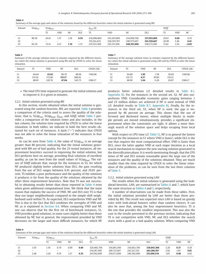
Table 4

Summary of the average gaps and values of the solutions found by the different heuristics when the initial solution is generated using RH.

Dataset %Gapinit %Gapfinal Zfinal ($) %Diff

TS VND NF DLS TS VND NF DLS TS VND NF

S1 80.30 26.61 1.37 1.28 0.59 236,906,800 335,207,600 334,990,700 337,503,800 29.81 0.68 0.74

S2 – – – – – 176,361,433 228,359,767 240,575,667 241,558,667 26.99 5.46 0.41

S3 83.70 13.15 4.13 1.70 1.75 219,333,300 242,151,500 248,291,000 248,173,200 11.62 2.43 −0.05

Table 5

Summary of the average solution times in minutes required by the different heuris-

tics when the initial solution is generated using RH and by CPLEX to solve the linear

relaxation.

Dataset TS VND NF DLS CPLEX (LR)

S1 64.64 43.62 90.76 88.96 1169.98

S2 135.41 172.86 115.17 688.41 –

S3 88.85 120.76 47.04 245.75 2186.17

5

e

a

t

v

l

r

t

w

w

g

a

p

D

q

u

N

f

c

i

o

f

w

r

t

b

T

N

o

V

o

d

Table 7

Summary of the average solution times in minutes required by the different heuris-

tics when the initial solution is generated using LAH and by CPLEX to solve the linear

relaxation.

Dataset TS VND NF DLS CPLEX (LR)

S1 64.80 1.99 7.58 30.69 1169.98

S2 135.72 4.57 30.89 116.12 –

S3 88.99 1.04 6.28 26.87 2186.17

p

A

p

a

(

s

p

F

p

p

o

o

(

o

D

s

t

t

i

s

a

o

5

a

t

t

v

r

a

t

c

T

s

• The total CPU time required to generate the initial solution and

to improve it. It is given in minutes.

.2.1. Initial solution generated using RH

In this section, results obtained when the initial solution is gen-

rated using the random heuristic, RH, are reported. Table 4 provides

comparison of the criteria used to assess the quality of the solu-

ions; that is, %Gapinit, %Gapfinal, Zfinal, and %Diff, while Table 5 pro-

ides a comparison of the solution times and also includes, in the

ast column, the solution time required by CPLEX to solve the linear

elaxation. In both tables, we indicate in bold the best results ob-

ained for each set of instances. A dash (“–”) indicates that CPLEX

as not able to solve the linear relaxation of the instances in four

eeks.

As can be seen from Table 4, the value of %Gapinit is on average

reater than 80 percent, indicating that the initial solutions gener-

ted with RH are of bad quality. For the 23 tested instances, all im-

rovement heuristics succeed in improving the initial solution, but

LS performs best on average, providing final solutions of excellent

uality, as can be seen from the small values of %Gapfinal. The val-

es of %Diff indicate that, except for the instances in S3, for which

F produced slightly better solutions than DLS, the gain resulting

rom the use of DLS ranges between 0.41 percent, and 29.81 per-

ent. TS exhibits a poor performance and the quality of the solutions

t produces is far from the quality of the solutions obtained by the

ther three improvement heuristics. Note that TS was not success-

ul in obtaining results better than those reported in Table 4 even

hen given additional computational time. We think that the main

eason that explains the success of VND, NF, and DLS over TS is that

hey use larger neighborhoods compared to the simple shift neigh-

orhood used within TS. As expected, DLS outperforms VND and NF.

his is due to the fact that DLS combines the strengths of VND and

F, as is explained in Section 4.4. When comparing VND and NF,

ne can observe that for the first set of benchmark instances, S1,

ND provides good solutions, in some cases slightly better than those

btained by NF, but in general, the improvement provided by VND

ecreases on the larger and more difficult instances, for which NF

Table 6

Summary of the average gaps and values of the solutions found by the different heuristics w

Dataset %Gapinit %Gapfinal Zfinal ($)

TS VND NF DLS TS

S1 1.59 1.39 0.79 0.99 0.40 320,466,700

S2 – – – – – 236,187,300

S3 2.40 2.26 0.76 1.27 0.35 247,042,000

roduces better solutions (cf. detailed results in Table B.1,

ppendix B). For the instances in the second set, S2, NF also out-

erforms VND. Considerable economic gains ranging between 1

nd 23 million dollars are achieved if NF is used instead of VND

cf. detailed results in Table B.7, Appendix B). Finally, for the in-

tances in the third set, S3, when NF is used, the gap is im-

roved by 46 percent on average. This shows that the use of

orward and Backward moves, where multiple blocks in multi-

le periods are moved simultaneously, provides a significant im-

rovement when the constraints are tight. It allows a more thor-

ugh search of the solution space and helps escaping from local

ptima.

With respect to CPU time (cf. Table 5), NF is in general the fastest

except for the instances in S1 where VND is faster), while DLS is the

ne that requires the most computational effort. VND is faster than

LS, since the latter applies VND at each major iteration as a local

earch mechanism to improve the new starting solution generated in

he diversification phase. It is worth mentioning though, that the CPU

imes of NF and DLS remain reasonable given the large size of the

nstances and the quality of the solutions obtained. They are much

maller than the time required by CPLEX to solve the linear relax-

tion of the problems, as can be seen from the last three columns

f Table 5.

.2.2. Initial solution generated using LAH

The results when the initial solution is generated using the look-

head heuristic, LAH, are summarized in Tables 6 and 7, which have

he same structure as Tables 4 and 5, respectively.

A number of observations can be made from these tables. First,

he initial solutions provided by LAH are better than those pro-

ided by RH. This result was expected since LAH is based on greedy

ules with look-ahead features rather than random choices. It can

lso be seen that, among the four improvement heuristics, TS is

he one that provides the smallest improvement. This was also the

ase in the results presented in the previous section, indicating that

S is not competitive with VND, NF, and DLS whether the search

tarts with a good or a bad quality solution. When comparing VND

hen the initial solution is generated using LAH.

%Diff

VND NF DLS TS VND NF

336,801,300 336,063,700 338,045,300 5.20 0.37 0.59

240,727,667 241,327,333 243,286,567 2.92 1.05 0.81

250,671,600 249,382,600 251,690,534 1.85 0.40 0.92

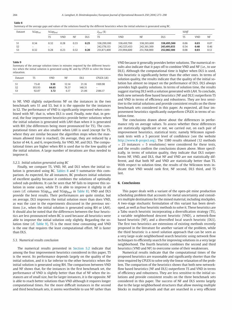
284 A. Lamghari, R. Dimitrakopoulos / European Journal of Operational Research 250 (2016) 273–290

Table 8

Summary of the average gaps and values of the solutions found by the different heuristics when the initial solution is generated using BC.

Dataset %Gapinit %Gapfinal Zfinal ($) %Diff

TS VND NF DLS TS VND NF DLS TS VND NF

S1 0.34 0.32 0.28 0.33 0.25 338,299,100 338,410,700 338,265,600 338,495,500 0.06 0.03 0.07

S2 – – – – – 242,178,133 242,525,433 242,361,300 243,491,033 0.54 0.40 0.46

S3 0.32 0.28 0.23 0.32 0.20 251,871,400 251,994,600 251,768,900 252,082,100 0.08 0.03 0.12

Table 9

Summary of the average solution times in minutes required by the different heuris-

tics when the initial solution is generated using BC and by CPLEX to solve the linear

relaxation.

Dataset TS VND NF DLS CPLEX (LR)

S1 73.41 9.10 12.14 21.16 1169.98

S2 193.93 64.65 76.37 148.31 –

S3 92.07 3.72 6.17 21.06 2186.17

V

s

D

t

s

l

p

s

b

a

t

b

p

l

m

a

i

r

h

×a

i

f

f

W

d

l

6

s

e

A

o

a

a

b

T

p

t

a

t

n

h

p

t

l

fl

o

l

c

d

b

to NF, VND slightly outperforms NF on the instances in the two

benchmark sets S1 and S3, but it is the opposite for the instances

in S2. The performance of VND is significantly improved when com-

bined with NF; that is, when DLS is used. Finally, note that, in gen-

eral, the four improvement heuristics provide better solutions when

the initial solution is generated with LAH than when it is generated

with RH (the differences being more pronounced for TS). The com-

putational times are also smaller when LAH is used (except for TS,

where they are similar because the algorithm stops when the max-

imum allowed time is reached). On average, they are reduced by a

factor of 44, 6, and 6, respectively, for VND, NF, and DLS. The compu-

tational times are higher when RH is used due to the low quality of

the initial solution. A large number of iterations are thus needed to

improve it.

5.2.3. Initial solution generated using BC

Finally, we compare TS, VND, NF, and DLS when the initial so-

lution is generated using BC. Tables 8 and 9 summarize this com-

parison. As expected, for all instances, BC produces initial solutions

of excellent quality because it combines the solutions of optimally

solved sub-problems. It can be seen that NF fails to improve this so-

lution in some cases, while TS is able to improve it slightly in all

cases (cf. columns %Gapinit and %Gapfinal in Table 8). VND and DLS

provide the best results. Their performances are quite similar, but

on average, DLS improves the initial solution more than does VND,

as was the case in the experiments discussed in the previous sec-

tions (i.e., when the initial solution is generated using RH or LAH).

It should also be noted that the differences between the four heuris-

tics are less pronounced when BC is used because all heuristics were

able to improve the initial solution only slightly. Regarding the so-

lution time (cf. Table 9), TS is the most time consuming and VND

is the one that requires the least computational effort. NF is faster

than DLS.

5.3. Numerical results conclusion

The numerical results presented in Section 5.2 indicate that

among the four improvement heuristics considered in this paper, TS

is the worst. Its performance depends largely on the quality of the

initial solution, and it is far inferior to the other heuristics when the

initial solution is generated using RH. The comparison between VND

and NF shows that, for the instances in the first benchmark set, the

performance of VND is slightly better than that of NF when the in-

stances are of small size, but for larger instances, it is the opposite. NF

is able to reach better solutions than VND although it requires longer

computational times. For the more difficult instances in the second

and third benchmark sets, it seems worthwhile to use NF rather than

ND because it generally provides better solutions. The numerical re-

ults also indicate that it pays off to combine VND and NF (i.e., to use

LS). Although the computational time is higher when DLS is used,

his heuristic is significantly better than the other ones. In terms of

olution quality, the results indicate that the quality of the initial so-

ution has almost no impact on the performance of DLS. DLS always

rovides high quality solutions. In terms of solution time, the results

uggest starting DLS with a solution generated with LAH. To conclude,

oth new network-flow based heuristics (NF and DLS) outperform TS

nd VND in terms of efficiency and robustness. They are less sensi-

ive to the initial solutions and provide consistent results on the three

enchmark sets considered in this paper. As expected, all four im-

rovement heuristics significantly outperform CPLEX in terms of so-

ution time.

The conclusions drawn above about the differences in perfor-

ance rely on average values. To assess whether these differences

re statistically significant or not, we carried out, on each pair of

mprovement heuristics, statistical tests; namely Wilcoxon signed-

ank tests with a 5 percent level of confidence (see the website

ttp://www.R-project.org). The 1380 results obtained (12 methods

23 instances × 5 resolutions) were considered for these tests,

nd the results confirm the conclusions drawn above. More specif-

cally, in terms of solution quality, they indicate that DLS outper-

orms NF, VND, and DLS, that NF and VND are not statistically dif-

erent, and that both NF and VND are statistically better than TS.

ith respect to solution time, the results of the Wilcoxon tests in-

icate that VND would rank first, NF second, DLS third, and TS

ast.

. Conclusions

This paper deals with a variant of the open-pit mine production

cheduling problem that accounts for metal uncertainty and consid-

rs multiple destinations for the mined material, including stockpiles.

two-stage stochastic formulation of this variant has been devel-

ped, as well as four heuristic methods to solve it. These heuristics are

Tabu search heuristic incorporating a diversification strategy (TS),

variable neighborhood descent heuristic (VND), a network-flow

ased heuristic (NF), and a diversified local search heuristic (DLS).

he first two heuristics are extensions of existing methods recently

roposed in the literature for another variant of the problem, while

he third heuristic is a novel solution approach that can be seen as

very large-scale neighborhood search heuristic using network flow

echniques to efficiently search for improving solutions in a very large

eighborhood. The fourth heuristic combines the second and third

euristics (VND and NF) to overcome some of their weaknesses.

Numerical results indicate that the computational times of the

roposed heuristics are reasonable and significantly shorter than the

ime required by CPLEX to solve only the linear relaxation of the prob-

em. The comparison of the heuristics shows that both new network-

ow based heuristics (NF and DLS) outperform TS and VND in terms

f efficiency and robustness. They are less sensitive to the initial so-

utions and provide consistent results on the three benchmark sets

onsidered in this paper. The success of NF and DLS seems largely

ue to the large neighborhood structures that allow moving multiple

locks in multiple periods and that are searched in a very efficient

A. Lamghari, R. Dimitrakopoulos / European Journal of Operational Research 250 (2016) 273–290 285

m

d

c

c

r

s

a

A

N

t

B

s

t

t

A

t

T

C

Table A.2

Characteristics of the three instances in the second set of benchmark instances, S2.

Instance Number of

blocks (N)

Number of

periods (T) in

years

Number of

scenarios (S)

S2–C1

Metal type: copper

Block size: 15 × 15 × 15 meters 14,118 6 25

Block weight: variable

5805 ≤ wi ≤ 9213.75 tonnes

S2–C2

Metal type: copper

Block size: 20 × 20 × 10 meters 28,154 16 20

Block weight: wi = 10, 800 tonnes

S2–G1

Metal type: gold

Block size: 15 × 15 × 10 meters 48,821 14 20

Block weight: wi = 5625 tonnes

Table A.3

Characteristics of the 10 instances in the third set of benchmark instances, S3.

Instance Number of

blocks (N)

Number of

periods (T) in

years

Number of

scenarios (S)

S3–C1

Metal type: copper

Block size: 20 × 20 × 10 meters 22,549 12 20

anner. When comparing DLS and NF, the results indicate that DLS

ominates in terms of solution quality. For all tested instances, DLS

an reach solutions with an average optimality gap of less than 2 per-

ent independently of the quality of the initial solution.

DLS and NF are flexible enough to handle other constraints. Future

esearch will be devoted to adapting them to solve more complex ver-

ions of the problem that include additional operational constraints

nd other sources of uncertainty.

cknowledgments

The work in this paper was funded by NSERC CRDPJ 411270-10,

SERC Discovery Grant 239019-06, and the industry members of

he COSMO Stochastic Mine Planning Laboratory: AngloGold Ashanti,

arrick Gold, BHP Billiton, De Beers, Newmont Mining, and Vale. This

upport is gratefully acknowledged. The authors would like to thank

hree anonymous referees for their valuable comments and sugges-

ions that helped improve the paper.

ppendix A. Detailed characteristics of the benchmark instances

Tables A.1–A.3 show the characteristics of the instances in the

hree datasets used in the numerical experiments.

able A.1

haracteristics of the 10 instances in the first set of benchmark instances, S1.

Instance Number of

blocks (N)

Number of

periods (T)

in years

Number of

scenarios

(S)

S1–C1

Metal type: copper

Block size: 20 × 20 × 10 meters 4,273 3 20

Block weight: wi = 10, 800 tonnes

S1–C2

Metal type: copper

Block size: 20 × 20 × 10 meters 7,141 4 20

Block weight: wi = 10, 800 tonnes

S1–C3

Metal type: copper

Block size: 20 × 20 × 10 meters 12,627 7 20

Block weight: wi = 10, 800 tonnes

S1–C4

Metal type: copper

Block size: 20 × 20 × 10 meters 20,626 10 20

Block weight: wi = 10, 800 tonnes

S1–C5

Metal type: copper

Block size: 20 × 20 × 10 meters 26,021 13 20

Block weight: wi = 10, 800 tonnes

S1–G1

Metal type: gold

Block size: 15 × 15 × 10 meters 18,821 5 20

Block weight: wi = 5625 tonnes

S1–G2

Metal type: gold

Block size: 15 × 15 × 10 meters 23,901 7 20

Block weight: wi = 5625 tonnes

S1–G3

Metal type: gold

Block size: 15 × 15 × 10 meters 30,013 8 20

Block weight: wi = 5625 tonnes

S1–G4

Metal type: gold

Block size: 15 × 15 × 10 meters 34,981 9 20

Block weight: wi = 5625 tonnes

S1–G5

Metal type: gold

Block size: 15 × 15 × 10 meters 40,762 11 20

Block weight: wi = 5625 tonnes

Block weight: wi = 10, 000 tonnes

S3–C2

Metal type: copper

Block size: 20 × 20 × 10 meters 22,388 12 20

Block weight: wi = 10, 000 tonnes

S3–C3

Metal type: copper

Block size: 20 × 20 × 10 meters 22,285 12 20

Block weight: wi = 10, 000 tonnes

S3–C4

Metal type: copper

Block size: 20 × 20 × 10 meters 22,302 12 20

Block weight: wi = 10, 000 tonnes

S3–C5

Metal type: copper

Block size: 20 × 20 × 10 meters 21,965 11 20

Block weight: wi = 10, 000 tonnes

S3–C6

Metal type: copper

Block size: 20 × 20 × 10 meters 22,246 12 20

Block weight: wi = 10, 000 tonnes

S3–C7

Metal type: copper

Block size: 20 × 20 × 10 meters 22,716 12 20

Block weight: wi = 10, 000 tonnes

S3–C8

Metal type: copper

Block size: 20 × 20 × 10 meters 22,529 12 20

Block weight: wi = 10, 000 tonnes

S3–C9

Metal type: copper

Block size: 20 × 20 × 10 meters 22,253 12 20

Block weight: wi = 10, 000 tonnes

S3–C10

Metal type: copper

Block size: 20 × 20 × 10 meters 22,720 12 20

Block weight: wi = 10, 000 tonnes

A

fi

t

B

n

b

i

i

ppendix B. Detailed computational results

Tables B.1–B.6 show the detailed results for each instance in the

rst dataset, S1. Detailed results for each instance in the second and

hird datasets (S2 and S3) are given in Tables B.7–B.12 and B.13–

.18, respectively. In addition to the initial gap (%Gapinit) and the fi-

al gap (%Gapfinal), for each method and each instance, we report the

est final gap out of the 5 runs (denoted by %Best Gap). Finally, as

n Section 5.2, we indicate in bold the best results obtained for each

nstance.

286 A. Lamghari, R. Dimitrakopoulos / European Journal of Operational Research 250 (2016) 273–290

Table B.1

Comparison of the gaps obtained by TS, VND, NF, and DLS on the instances in S1 when the initial solution is generated using RH

Instance N T %Gapinit %Gapfinal %Best Gap

TS VND NF DLS TS VND NF DLS

S1–C1 4,273 3 58.882 6.926 0.125 0.633 0.030 5.801 0.061 0.529 0.020

S1–C2 7,141 4 62.181 15.398 0.292 0.818 0.109 11.225 0.203 0.743 0.082

S1–C3 12,627 7 70.822 19.845 0.978 1.272 0.345 17.523 0.738 1.018 0.255

S1–C4 20,626 10 81.726 25.572 3.145 1.650 1.069 21.259 2.967 1.426 0.978

S1–C5 26,021 13 89.062 19.076 4.922 1.677 1.752 16.922 4.630 1.328 1.574

S1–G1 18,821 5 83.498 27.486 0.349 0.977 0.304 14.444 0.349 0.815 0.277

S1–G2 23,901 7 86.063 47.929 0.593 1.373 0.482 41.156 0.513 1.238 0.459

S1–G3 30,013 8 88.118 37.099 0.709 1.176 0.505 27.756 0.709 1.091 0.468

S1–G4 34,981 9 89.855 34.405 0.856 1.570 0.517 23.036 0.779 1.210 0.490

S1–G5 40,762 11 92.820 32.400 1.770 1.686 0.800 25.554 1.678 1.567 0.749

Table B.2

Comparison between the solution times required by TS, VND, NF, and DLS when the initial solution is gen-

erated using RH and the time required by CPLEX to solve the linear relaxation (instances in S1). The times

are given in minutes.

Instance N T TS VND NF DLS CPLEX (LR)

S1–C1 4,273 3 4.27 1.05 3.26 1.91 0.23

S1–C2 7,141 4 9.52 3.26 8.09 4.90 5.68

S1–C3 12,627 7 29.46 13.00 19.29 24.52 139.01

S1–C4 20,626 10 68.76 43.95 45.20 88.86 1540.61

S1–C5 26,021 13 112.76 72.91 55.06 145.25 3470.63

S1–G1 18,821 5 31.36 17.34 78.97 37.95 187.77

S1–G2 23,901 7 55.78 31.92 100.71 54.03 323.75

S1–G3 30,013 8 80.04 57.29 168.68 109.94 2459.00

S1–G4 34,981 9 104.95 80.46 188.84 161.45 1179.05

S1–G5 40,762 11 149.47 115.06 239.51 260.78 2394.03

Table B.3

Comparison of the gaps obtained by TS, VND, NF, and DLS on the instances in S1 when the initial solution is generated using LAH.

Instance N T %Gapinit %Gapfinal %Best Gap

TS VND NF DLS TS VND NF DLS

S1–C1 4,273 3 1.054 0.804 0.293 0.608 0.040 0.606 0.293 0.608 0.029

S1–C2 7,141 4 1.497 1.183 0.423 0.705 0.046 1.000 0.423 0.705 0.043

S1–C3 12,627 7 1.326 1.178 0.542 0.908 0.252 1.151 0.461 0.908 0.237

S1–C4 20,626 10 3.025 2.683 1.920 1.393 0.750 2.568 1.888 1.393 0.641

S1–C5 26,021 13 2.458 2.251 1.087 1.331 0.607 2.227 1.069 1.331 0.579

S1–G1 18,821 5 0.638 0.590 0.393 0.638 0.284 0.590 0.393 0.638 0.284

S1–G2 23,901 7 0.910 0.872 0.521 0.910 0.444 0.868 0.521 0.910 0.432

S1–G3 30,013 8 1.035 1.000 0.648 1.035 0.470 0.992 0.648 1.035 0.464

S1–G4 34,981 9 2.016 1.734 1.175 1.137 0.484 1.734 1.175 1.137 0.470

S1–G5 40,762 11 1.909 1.562 0.912 1.290 0.613 1.528 0.912 1.290 0.601

Table B.4

Comparison between the solution times required by TS, VND, NF, and DLS when the initial solution is

generated using LAH and the time required by CPLEX to solve the linear relaxation (instances in S1).

The times are given in minutes.

Instance N T TS VND NF DLS CPLEX (LR)

S1–C1 4,273 3 4.28 0.17 1.09 0.80 0.23

S1–C2 7,141 4 9.53 0.44 1.58 2.73 5.68

S1–C3 12,627 7 29.51 0.73 3.81 7.31 139.01

S1–C4 20,626 10 68.87 1.66 4.55 32.47 1540.61

S1–C5 26,021 13 112.94 2.23 8.91 32.60 3470.63

S1–G1 18,821 5 31.47 2.45 2.09 13.08 187.77

S1–G2 23,901 7 55.93 2.04 3.15 24.35 323.75

S1–G3 30,013 8 80.29 4.18 4.89 42.78 2459.00

S1–G4 34,981 9 105.28 3.40 21.09 64.24 1179.05

S1–G5 40,762 11 149.94 2.63 24.66 86.55 2394.03

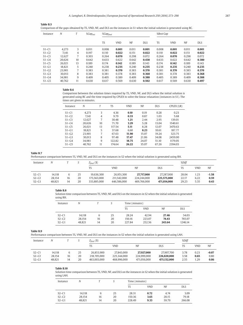
A. Lamghari, R. Dimitrakopoulos / European Journal of Operational Research 250 (2016) 273–290 287

Table B.5

Comparison of the gaps obtained by TS, VND, NF, and DLS on the instances in S1 when the initial solution is generated using BC.

Instance N T %Gapinit %Gapfinal %Best Gap

TS VND NF DLS TS VND NF DLS

S1–C1 4,273 3 0.011 0.008 0.001 0.011 0.001 0.008 0.001 0.011 0.001

S1–C2 7,141 4 0.197 0.110 0.022 0.151 0.022 0.110 0.022 0.151 0.022

S1–C3 12,627 7 0.303 0.264 0.070 0.298 0.072 0.264 0.070 0.298 0.072

S1–C4 20,626 10 0.642 0.633 0.622 0.642 0.430 0.633 0.622 0.642 0.380

S1–C5 26,021 13 0.189 0.174 0.142 0.189 0.143 0.174 0.142 0.189 0.143

S1–G1 18,821 5 0.240 0.238 0.235 0.240 0.235 0.238 0.235 0.240 0.235

S1–G2 23,901 7 0.383 0.381 0.370 0.383 0.370 0.381 0.370 0.383 0.370

S1–G3 30,013 8 0.383 0.381 0.378 0.383 0.368 0.381 0.378 0.383 0.368

S1–G4 34,981 9 0.409 0.405 0.389 0.409 0.388 0.405 0.389 0.409 0.388

S1–G5 40,762 11 0.630 0.617 0.569 0.630 0.502 0.617 0.569 0.630 0.497

Table B.6

Comparison between the solution times required by TS, VND, NF, and DLS when the initial solution is

generated using BC and the time required by CPLEX to solve the linear relaxation (instances in S1). The

times are given in minutes.

Instance N T TS VND NF DLS CPLEX (LR)

S1–C1 4,273 3 4.36 0.10 0.19 0.28 0.23

S1–C2 7,141 4 9.79 0.33 0.87 1.03 5.68

S1–C3 12,627 7 30.48 1.21 2.44 2.95 139.01

S1–C4 20,626 10 71.70 3.29 5.28 13.04 1540.61

S1–C5 26,021 13 117.54 5.11 8.28 12.07 3470.63

S1–G1 18,821 5 37.68 6.60 8.23 10.61 187.77

S1–G2 23,901 7 67.63 11.90 15.07 19.24 323.75

S1–G3 30,013 8 97.48 17.47 21.86 34.08 2459.00

S1–G4 34,981 9 122.82 18.75 24.07 51.10 1179.05

S1–G5 40,762 11 174.64 26.22 35.07 67.26 2394.03

Table B.7

Performance comparison between TS, VND, NF, and DLS on the instances in S2 when the initial solution is generated using RH.

Instance N T S Zfinal ($) %Diff

TS VND NF DLS TS VND NF

S2–C1 14,118 6 25 19,636,300 26,951,300 27,717,000 27,287,000 28.04 1.23 -1.58

S2–C2 28,154 16 20 175,563,000 211,542,000 224,244,000 225,575,000 22.17 6.22 0.59

S2–G1 48,821 14 20 333,885,000 446,586,000 469,766,000 471,814,000 29.23 5.35 0.43

Table B.8

Solution time comparison between TS, VND, NF, and DLS on the instances in S2 when the initial solution is generated

using RH.

Instance N T S Time (minutes)

TS VND NF DLS

S2–C1 14,118 6 25 28.24 42.94 27.46 54.03

S2–C2 28,154 16 20 150.16 223.07 74.43 765.07

S2–G1 48,821 14 20 227.84 252.56 243.64 1246.14

Table B.9

Performance comparison between TS, VND, NF, and DLS on the instances in S2 when the initial solution is generated using LAH.

Instance N T S Zfinal ($) %Diff

TS VND NF DLS TS VND NF

S2–C1 14,118 6 25 26,853,900 27,843,000 27,927,000 27,907,700 3.78 0.23 -0.07

S2–C2 28,154 16 20 218,705,000 225,344,000 224,999,000 226,820,000 3.58 0.65 0.80

S2–G1 48,821 14 20 463,003,000 468,996,000 471,056,000 475,132,000 2.55 1.29 0.86

Table B.10

Solution time comparison between TS, VND, NF, and DLS on the instances in S2 when the initial solution is generated

using LAH.

Instance N T S Time (minutes)

TS VND NF DLS

S2–C1 14,118 6 25 28.31 0.72 4.74 3.09

S2–C2 28,154 16 20 150.36 3.65 28.15 79.18

S2–G1 48,821 14 20 228.49 9.33 59.79 266.08

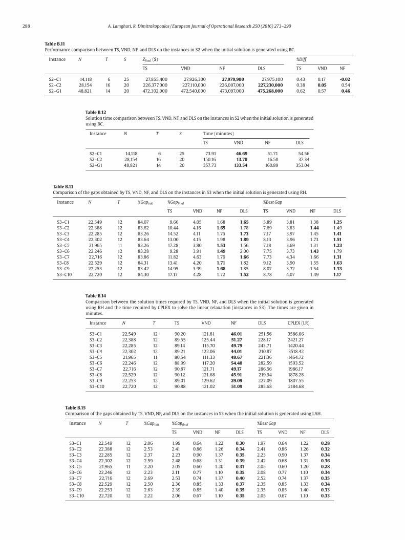
288 A. Lamghari, R. Dimitrakopoulos / European Journal of Operational Research 250 (2016) 273–290

Table B.11

Performance comparison between TS, VND, NF, and DLS on the instances in S2 when the initial solution is generated using BC.

Instance N T S Zfinal ($) %Diff

TS VND NF DLS TS VND NF

S2–C1 14,118 6 25 27,855,400 27,926,300 27,979,900 27,975,100 0.43 0.17 -0.02

S2–C2 28,154 16 20 226,377,000 227,110,000 226,007,000 227,230,000 0.38 0.05 0.54

S2–G1 48,821 14 20 472,302,000 472,540,000 473,097,000 475,268,000 0.62 0.57 0.46

Table B.12

Solution time comparison between TS, VND, NF, and DLS on the instances in S2 when the initial solution is generated

using BC.

Instance N T S Time (minutes)

TS VND NF DLS

S2–C1 14,118 6 25 73.91 46.69 51.71 54.56

S2–C2 28,154 16 20 150.16 13.70 16.50 37.34

S2–G1 48,821 14 20 357.73 133.54 160.89 353.04

Table B.13

Comparison of the gaps obtained by TS, VND, NF, and DLS on the instances in S3 when the initial solution is generated using RH.

Instance N T %Gapinit %Gapfinal %Best Gap

TS VND NF DLS TS VND NF DLS

S3–C1 22,549 12 84.07 9.66 4.05 1.68 1.65 5.89 3.81 1.38 1.25

S3–C2 22,388 12 83.62 10.44 4.16 1.65 1.78 7.69 3.83 1.44 1.49

S3–C3 22,285 12 83.26 14.52 4.11 1.76 1.73 7.17 3.97 1.45 1.41

S3–C4 22,302 12 83.64 13.00 4.15 1.98 1.89 8.13 3.96 1.73 1.51

S3–C5 21,965 11 83.26 17.28 3.80 1.53 1.56 7.18 3.69 1.31 1.23

S3–C6 22,246 12 83.28 9.28 3.91 1.49 2.00 7.75 3.73 1.43 1.79

S3–C7 22,716 12 83.86 11.82 4.63 1.79 1.66 7.73 4.34 1.66 1.31

S3-C8 22,529 12 84.31 13.41 4.20 1.71 1.82 9.12 3.90 1.55 1.63

S3–C9 22,253 12 83.42 14.95 3.99 1.68 1.85 8.07 3.72 1.54 1.33

S3–C10 22,720 12 84.30 17.17 4.28 1.72 1.52 8.78 4.07 1.49 1.17

Table B.14

Comparison between the solution times required by TS, VND, NF, and DLS when the initial solution is generated

using RH and the time required by CPLEX to solve the linear relaxation (instances in S3). The times are given in

minutes.

Instance N T TS VND NF DLS CPLEX (LR)

S3–C1 22,549 12 90.20 121.81 46.01 251.56 3586.66

S3–C2 22,388 12 89.55 125.44 51.27 228.17 2421.27

S3–C3 22,285 12 89.14 115.70 49.79 243.71 1420.44

S3–C4 22,302 12 89.21 122.06 44.01 210.87 3518.42

S3–C5 21,965 11 80.54 111.33 49.67 221.36 1464.72

S3–C6 22,246 12 88.99 117.20 54.40 282.59 1593.52

S3–C7 22,716 12 90.87 121.71 49.17 286.56 1986.17

S3–C8 22,529 12 90.12 121.68 45.91 219.94 1878.28

S3–C9 22,253 12 89.01 129.62 29.09 227.09 1807.55

S3–C10 22,720 12 90.88 121.02 51.09 285.68 2184.68

Table B.15

Comparison of the gaps obtained by TS, VND, NF, and DLS on the instances in S3 when the initial solution is generated using LAH.

Instance N T %Gapinit %Gapfinal %Best Gap

TS VND NF DLS TS VND NF DLS

S3–C1 22,549 12 2.06 1.99 0.64 1.22 0.30 1.97 0.64 1.22 0.28

S3–C2 22,388 12 2.53 2.41 0.86 1.26 0.34 2.41 0.86 1.26 0.32

S3–C3 22,285 12 2.37 2.23 0.90 1.37 0.35 2.23 0.90 1.37 0.34

S3–C4 22,302 12 2.59 2.48 0.68 1.31 0.39 2.42 0.68 1.31 0.36

S3–C5 21,965 11 2.20 2.05 0.60 1.20 0.31 2.05 0.60 1.20 0.28

S3–C6 22,246 12 2.23 2.11 0.77 1.10 0.35 2.08 0.77 1.10 0.34

S3–C7 22,716 12 2.69 2.53 0.74 1.37 0.40 2.52 0.74 1.37 0.35

S3–C8 22,529 12 2.50 2.36 0.85 1.33 0.37 2.35 0.85 1.33 0.34

S3–C9 22,253 12 2.63 2.39 0.85 1.40 0.35 2.35 0.85 1.40 0.33

S3–C10 22,720 12 2.22 2.06 0.67 1.10 0.35 2.05 0.67 1.10 0.33

A. Lamghari, R. Dimitrakopoulos / European Journal of Operational Research 250 (2016) 273–290 289

S, VN

e line

instan

ND

.23

.29

.19

.24

.23

.27

.27

.25

.21

.15

S, VN

linea

R

A

A

A

A

B

B

B

B

Table B.16

Comparison between the solution times required by T

using LAH and the time required by CPLEX to solve th

minutes.

Instance N T TS

S3–C1 22,549 12 90.34

S3–C2 22,388 12 89.69

S3–C3 22,285 12 89.28

S3–C4 22,302 12 89.35

S3–C5 21,965 11 80.67

S3–C6 22,246 12 89.12

S3–C7 22,716 12 91.01

S3–C8 22,529 12 90.26

S3–C9 22,253 12 89.15

S3–C10 22,720 12 91.02

Table B.17

Comparison of the gaps obtained by TS, VND, NF, and DLS on the

Instance N T %Gapinit %Gapfinal

TS V

S3–C1 22,549 12 0.29 0.27 0

S3–C2 22,388 12 0.48 0.38 0

S3–C3 22,285 12 0.27 0.23 0

S3–C4 22,302 12 0.31 0.30 0

S3–C5 21,965 11 0.25 0.24 0

S3–C6 22,246 12 0.29 0.28 0

S3–C7 22,716 12 0.47 0.38 0

S3–C8 22,529 12 0.28 0.27 0

S3–C9 22,253 12 0.35 0.28 0

S3–C10 22,720 12 0.21 0.18 0

Table B.18

Comparison between the solution times required by T

using BC and the time required by CPLEX to solve the

minutes.

Instance N T TS

S3–C1 22,549 12 93.29

S3–C2 22,388 12 92.94

S3–C3 22,285 12 92.02

S3–C4 22,302 12 92.54

S3–C5 21,965 11 83.55

S3–C6 22,246 12 91.81

S3–C7 22,716 12 94.33

S3–C8 22,529 12 93.72

S3–C9 22,253 12 92.60

S3–C10 22,720 12 93.95

eferences

huja, R. K., Ergun, O., Magnanti, T., & Orlin, J. (1993). Network flows: Theory, algorithms,and applications. Prentice Hall.

huja, R. K., Ergun, O., Orlin, J. B., & Punnen, A. P. (2002). A survey of very large-scaleneighborhood search techniques. Discrete Applied Mathematics, 123, 75–102.

lbor, F., & Dimitrakopoulos, R. (2009). Stochastic mine design optimization based on

simulated annealing: Pit limits, production schedules, multiple orebody scenariosand sensitivity analysis. IMM Transactions, Mining Technology, 118(2), 80–91.

lbor, F., & Dimitrakopoulos, R. (2010). Algorithmic approach to pushback design basedon stochastic programming: Method, application and comparisons. IMM Transac-

tions, Mining Technology, 119(2), 88–101.

D, NF, and DLS when the initial solution is generated

ar relaxation (instances in S3). The times are given in

VND NF DLS CPLEX (LR)

0.92 5.45 30.61 3586.66

0.95 6.40 23.64 2421.27

1.09 6.18 22.54 1420.44

1.06 7.59 21.14 3518.42

1.40 6.35 20.53 1464.72

0.90 6.45 63.96 1593.52

1.07 6.46 21.59 1986.17

1.08 5.73 17.10 1878.28

0.99 5.98 20.29 1807.55

0.91 6.16 27.31 2184.68

ces in S3 when the initial solution is generated using BC.

%Best Gap

NF DLS TS VND NF DLS

0.29 0.15 0.27 0.23 0.29 0.15

0.48 0.21 0.38 0.29 0.48 0.20

0.27 0.18 0.23 0.19 0.27 0.16

0.31 0.22 0.30 0.23 0.31 0.22

0.25 0.21 0.24 0.23 0.25 0.19

0.29 0.24 0.28 0.27 0.29 0.23

0.47 0.20 0.38 0.27 0.47 0.19

0.28 0.24 0.27 0.25 0.28 0.21

0.35 0.17 0.28 0.21 0.35 0.15

0.21 0.15 0.18 0.15 0.21 0.15

D, NF, and DLS when the initial solution is generated

r relaxation (instances in S3). The times are given in

VND NF DLS CPLEX (LR)

3.65 6.29 24.46 3586.66

3.89 6.50 29.03 2421.27

3.31 5.81 19.60 1420.44

3.82 6.04 13.87 3518.42

3.53 5.97 19.85 1464.72

3.19 5.58 17.79 1593.52

4.10 6.78 37.92 1986.17

3.98 6.39 18.27 1878.28

4.19 6.52 17.38 1807.55

3.53 5.80 12.43 2184.68

ehrang, K., Hooman, A., & Clayton, D. (2014). A linear programming model for long-term mine planning in the presence of grade uncertainty and a stockpile. Interna-

tional Journal of Mining Science and Technology, 24, 451–459.

ienstock, D., & Zuckerberg, M. (2010). Solving LP relaxations of large-scale precedenceconstrained problems. Lecture Notes in Computer Science, 6080, 1–14.

irge, J., & Louveaux, F. (2011). Introduction to stochastic programming (2nd ed.).Springer.

oland, N., Dumitrescu, I. Froyland, G. (2008). A multistage stochastic programming ap-proach to open pit mine production scheduling with uncertain geology. Optimiza-

tion Online. Last accessed: August 27, 2014. URL http://www.optimization-online.

org/DB_FILE/2008/10/2123.pdf.

290 A. Lamghari, R. Dimitrakopoulos / European Journal of Operational Research 250 (2016) 273–290

H

I

J

K

L

L

M

M

N

O

R

R

R

R

S

T

W

Boland, N., Dumitrescu, I., Froyland, G., & Gleixner, A. M. (2009). LP-based disaggre-gation approaches to solving the open pit mining production scheduling problem

with block processing selectivity. Computers & Operations Research, 36(4), 1064–1089.

Caccetta, L., & Hill, S. P. (2003). An application of branch and cut to open pit minescheduling. Journal of Global Optimization, 27, 349–365.

Chatterjee, S., Lamghari, A., & Dimitrakopoulos, R. (2010). A two-phase heuristicmethod for constrained pushback design. In R. Castro, X. Emery, & R. Kuyvenhoven

(Eds.), Proceedings of MININ 2010, conference on mining innovation, Santiago, Chile

(pp. 195–204).Chicoisne, R., Espinoza, D., Goycoolea, M., Moreno, E., & Rubio, E. (2012). A new algo-

rithm for the open-pit mine production scheduling problem. Operations Research,60(3), 517–528.

Dagdelen, K., & Johnson, T. B. (1986). Optimum open pit mine production schedulingby Lagrangian parameterization. In Proceedings of 19th international APCOM sympo-

sium, Littleton, CO (pp. 127–142).

Dimitrakopoulos, R. (2011). Stochastic optimization for strategic mine planning: Adecade of developments. Journal of Mining Science, 84, 138–150.

Dimitrakopoulos, R., Farrelly, C., & Godoy, M. (2002). Moving forward from traditionaloptimization: Grade uncertainty and risk effects in open pit mine design. IMM

Transactions, 111, A82–A88.Dimitrakopoulos, R., & Jewbali, A. (2013). Joint stochastic optimization of short- and

long-term mine production planning: Method and application in a large operating

gold mine. IMM Transactions, Mining Technology, 122(2), 110–123.Dowd, P. (1994). Risk assessment in reserve estimation and open-pit planning. Trans-

actions of the Institution of Mining and Metallurgy, 103, A148–A154.Dowd, P. (1997). Risk in minerals projects: Analysis, perception and management.

Transactions of the Institution of Mining and Metallurgy, 106, A9–A18.Ferland, J. A., Amaya, J., & Djuimo, M. S. (2007). Application of a particle swarm algo-

rithm to the capacitated open pit mining problem. In S. Mukhopadhyay, & G. Sen

Gupta (Eds.), Autonomous robots and agents (pp. 127–133). Springer-Verlag.Gendreau, M. (2003). An introduction to tabu search. In F. Glover, & G. Kochenberger

(Eds.), Handbook of metaheuristics (pp. 37–54). Boston: Kluwer.Gershon, M. (1987). Heuristic approaches for mine planning and production schedul-

ing. International Journal of Mining and Geological Engineering, 5(1), 1–13.Glover, F. (1996). Ejection chains, reference structures and alternating path methods

for traveling salesman problems. Discrete Applied Mathematics, 65, 223–253.

Godoy, M. (2003). The effective management of geological risk, Ph.D. thesis. Australia:University of Queensland.

Godoy, M., & Dimitrakopoulos, R. (2004). Managing risk and waste mining in long-termproduction scheduling of open-pit mines. SME Transactions, 316, 43–50.

Goodfellow, R., & Dimitrakopoulos, R. (2013). Algorithmic integration of geological un-certainty in pushback designs for complex multi-process open-pit mines. Mining

Technology, 122(2), 67–77.

Goovaerts, P. (1997). Geostatistics for natural resources evaluation. Oxford UniversityPress.

ochbaum, D., & Chen, A. (2000). Improved planning for the open-pit mining problem.Operations Research, 48(6), 894–914.

BM (2010). Ibm ilog ampl version 12.2 user’s guide: Standard (command-line) versionincluding cplex directives.

ohnson, T. B. (1969). Optimum production scheduling. In Proceedings of the 8th interna-tional symposium on computers and operations research, Salt Lake City (pp. 539–562).

ent, M., Peattie, R., & Chamberlain, V. (2007). Incorporating grade uncertainty in thedecision to expand the main pit at the Navachab gold mine, Namibia, through the

use of stochastic simulation. The Australasian Institute of Mining and Metallurgy,

Spectrum Series, 14, 207–218.amghari, A., & Dimitrakopoulos, R. (2012). A diversified tabu search approach for the

open-pit mine production scheduling problem with metal uncertainty. EuropeanJournal of Operational Research, 222, 642–652.

amghari, A., Dimitrakopoulos, R., & Ferland, J. A. (2014). A variable neighbourhood de-scent algorithm for the open-pit mine production scheduling problem with metal

uncertainty. Journal of the Operational Research Society, 65, 1305–1314.

arcotte, D., & Caron, J. (2013). Ultimate open pit stochastic optimization. Computers& Geosciences, 51, 238–246.

enabde, M., Froyland, G., Stone, P., & Yeates, G. (2005). Mining schedule optimisa-tion for conditionally simulated orebodies. In Orebody modelling and strategic mine

planning: Uncertainty and risk management models (pp. 353–357). Australasian In-stitute of Mining and Metallurgy.

ewman, A. M., Rubio, E., Caro, R., Weintraub, A., & Eurek, K. (2010). A review of oper-

ations research in mine planning. Interfaces, 40(3), 222–245.sanloo, M., Gholamnejad, J., & Karimi, B. (2008). Long-term open pit mine produc-

tion planning: A review of models and algorithms. International Journal of Mining,Reclamation and Environment, 22, 3–53.

amazan, S. (2007). The new fundamental tree algorithm for production scheduling ofopen pit mines. European Journal of Operational Research, 177, 1153–1166.

amazan, S., & Dimitrakopoulos, R. (2013). Production scheduling with uncertain sup-

ply: A new solution to the open pit mining problem. Optimization and Engineering,14(2), 361–380.

avenscroft, P. (1992). Risk analysis for mine scheduling by conditional simulation.Transactions of the Institution of Mining and Metallurgy, Section A: Mining Technology,

101, A104–A108.emy, N., Boucher, A., & Wu, J. (2009). Applied geostatistics with SGeMS. Cambridge Uni-

versity Press.

evim, H., & Lei, D. (1998). The problem of production planning in open pit mines.INFOR, 36(1–2), 1–12.

olwinski, B., & Underwood, R. (1996). A scheduling algorithm for open pit mines. IMAJournal of Mathematics Applied in Business & Industry, 7, 247–270.

hittle, D., & Bozorgebrahimi, A. (2005). Hybrid pits – linking conditional simulationand Lerchs–Grossmann through set theory. In Orebody modelling and strategic mine

planning: Uncertainty and risk management models (pp. 37–42). Australasian Insti-

tute of Mining and Metallurgy.