network design performance evaluation, and simulationnetwork performance... 1 network design...
TRANSCRIPT
1Network Performance...
Network Design
Performance Evaluation, and
Simulation
#6
2Network Performance...
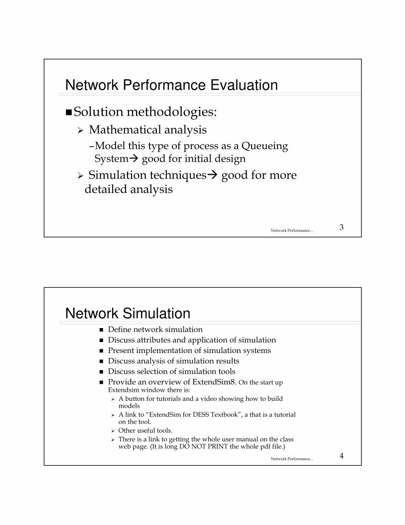
Network Design Problem� Goal
� Given – QoS metric, e.g.,
� Average delay� Loss probability
– Characterization of the traffic, e.g.,� Average interarrival time (arrival rate)� Average holding time (message length)
� Design the system � Three systems will be studied:
– Circuit switch, e.g., determine the # lines � System 1 �M/M/S/S (M/M/S/S /∞)
– Ideal router output port, e.g., determine link capacity �System 2 �M/M/1 (M/M/1/∞/∞)
– Real router output port, e.g., determine link capacity and buffer size � System 3 �M/M/1/N (M/M/1/N /∞)
3Network Performance...
Network Performance Evaluation
�Solution methodologies:
� Mathematical analysis
–Model this type of process as a Queueing System� good for initial design
� Simulation techniques� good for more detailed analysis
4Network Performance...
Network Simulation� Define network simulation
� Discuss attributes and application of simulation
� Present implementation of simulation systems
� Discuss analysis of simulation results
� Discuss selection of simulation tools
� Provide an overview of ExtendSim8. On the start up Extendsim window there is:
� A button for tutorials and a video showing how to build models
� A link to “ExtendSim for DESS Textbook”, a that is a tutorial on the tool.
� Other useful tools.
� There is a link to getting the whole user manual on the class web page. (It is long DO NOT PRINT the whole pdf file.)
5Network Performance...
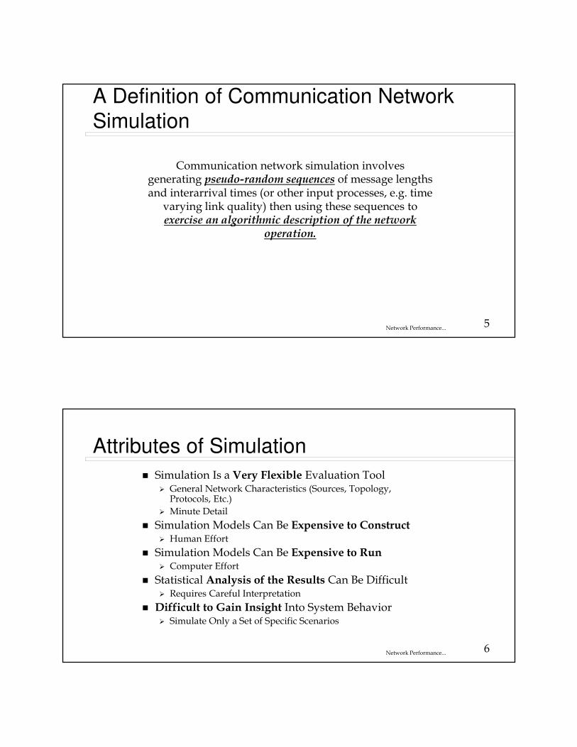
A Definition of Communication Network
Simulation
Communication network simulation involves generating pseudo-random sequences of message lengths and interarrival times (or other input processes, e.g. time
varying link quality) then using these sequences to exercise an algorithmic description of the network
operation.
6Network Performance...
Attributes of Simulation
� Simulation Is a Very Flexible Evaluation Tool� General Network Characteristics (Sources, Topology, Protocols, Etc.)
� Minute Detail
� Simulation Models Can Be Expensive to Construct� Human Effort
� Simulation Models Can Be Expensive to Run� Computer Effort
� Statistical Analysis of the Results Can Be Difficult� Requires Careful Interpretation
� Difficult to Gain Insight Into System Behavior� Simulate Only a Set of Specific Scenarios
7Network Performance...
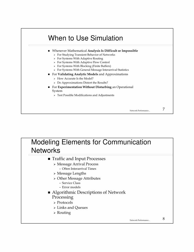
When to Use Simulation
� Whenever Mathematical Analysis Is Difficult or Impossible� For Studying Transient Behavior of Networks
� For Systems With Adaptive Routing
� For Systems With Adaptive Flow Control
� For Systems With Blocking (Finite Buffers)
� For Systems With General Message Interarrival Statistics
� For Validating Analytic Models and Approximations
� How Accurate Is the Model?
� Do Approximations Distort the Results?
� For Experimentation Without Disturbing an Operational System
� Test Possible Modifications and Adjustments
8Network Performance...
Modeling Elements for Communication
Networks� Traffic and Input Processes
� Message Arrival Process– Often Interarrival Times
� Message Lengths
� Other Message Attributes– Service Class
– Error models
� Algorithmic Descriptions of Network Processing� Protocols
� Links and Queues
� Routing
9Network Performance...
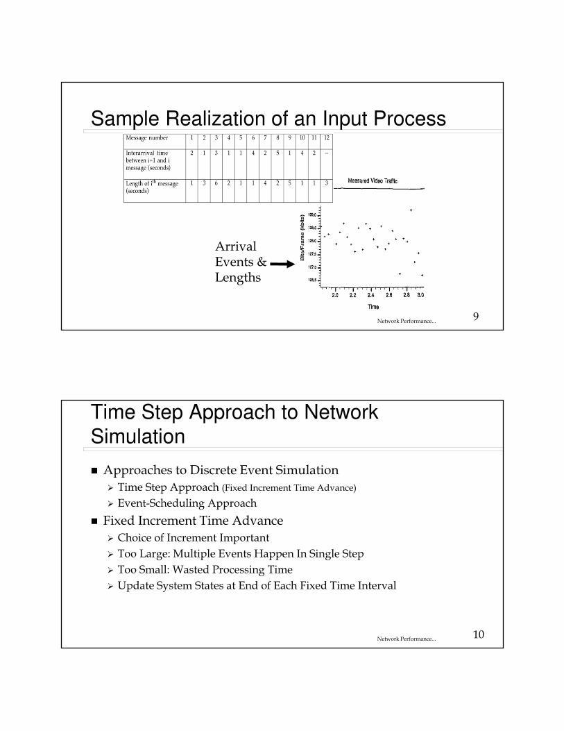
Sample Realization of an Input Process
ArrivalEvents &Lengths
10Network Performance...
Time Step Approach to Network
Simulation
� Approaches to Discrete Event Simulation
� Time Step Approach (Fixed Increment Time Advance)
� Event-Scheduling Approach
� Fixed Increment Time Advance
� Choice of Increment Important
� Too Large: Multiple Events Happen In Single Step
� Too Small: Wasted Processing Time
� Update System States at End of Each Fixed Time Interval
11Network Performance...
Event Scheduling Approach to Network
Simulation� Variable Time Advance
� Advance Time To Next Occurring Event
� Update System State Only When Events Occur� For Example, Arrivals or Departures
� Event Calendar� Events: Instantaneous Occurrences That Change the State of the System
� An Event is Described by
– The Time the Event is to Occur
– The Activity to Take Place at the Event Time
� The Calendar is a Time-Ordered List of Events
12Network Performance...
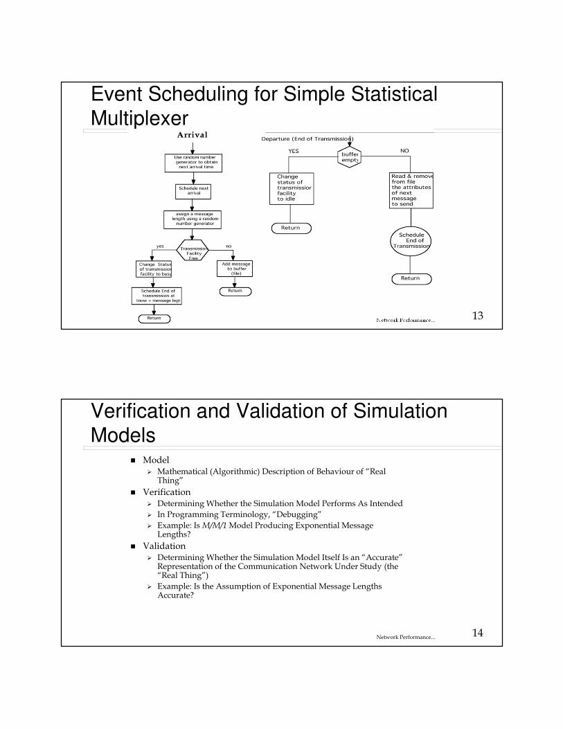
Event Scheduling Approach: Simplified
Flow Control
An Executive (or Mainline) Controls the Selection of Next Event
Use Event Listto determine next event to process
Advance simulation clock to event time
Update system stateusing event routines
Update event listusing event routines
13Network Performance...
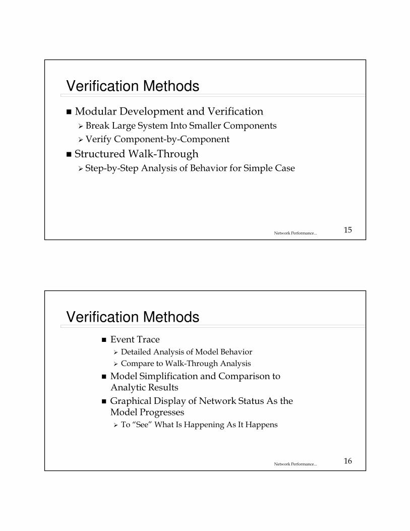
Event Scheduling for Simple Statistical
Multiplexer
14Network Performance...
Verification and Validation of Simulation
Models� Model
� Mathematical (Algorithmic) Description of Behaviour of “Real Thing”
� Verification� Determining Whether the Simulation Model Performs As Intended
� In Programming Terminology, “Debugging”
� Example: Is M/M/1Model Producing Exponential Message Lengths?
� Validation� Determining Whether the Simulation Model Itself Is an “Accurate”
Representation of the Communication Network Under Study (the “Real Thing”)
� Example: Is the Assumption of Exponential Message Lengths Accurate?
15Network Performance...
Verification Methods
� Modular Development and Verification
� Break Large System Into Smaller Components
�Verify Component-by-Component
� Structured Walk-Through
� Step-by-Step Analysis of Behavior for Simple Case
16Network Performance...
Verification Methods
� Event Trace
� Detailed Analysis of Model Behavior
� Compare to Walk-Through Analysis
� Model Simplification and Comparison to Analytic Results
� Graphical Display of Network Status As the Model Progresses
� To “See” What Is Happening As It Happens

17Network Performance...
Some Comments on Validation� Simulation Models Are Always Approximations
� A Simulation Model Developed for One Application May Not Be Valid for Others
� Model Development and Validation Should Be Done Simultaneously
� Specific Modeling Assumptions Should Be Tested
� Sensitivity Analysis Should Be Performed
� Attempt to Establish That the Model Results Resemble the Expected Performance of the Actual System
� Generally, Validation Is More Difficult Than Verification
18Network Performance...
Analysis of Results: Statistical
Considerations
� Starting Rules� Overcoming Initial Transients
� An Initial Transient Period Is Present Which Can Bias the Results
� Achieving Steady State
– Use a Run-in Period:� Determine Tb Such That the Long-Run Distribution Adequately Describes the System for t > Tb
– Use a “Typical” Starting Condition (State) to Initialize the Model
� Quality of Performance Estimates� Variance of Estimated Performance Measures
19Network Performance...
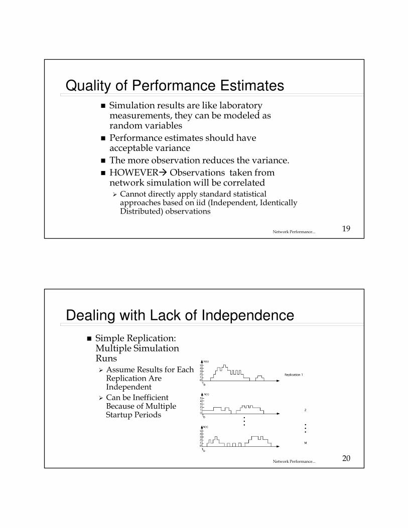
Quality of Performance Estimates
� Simulation results are like laboratory measurements, they can be modeled as random variables
� Performance estimates should have acceptable variance
� The more observation reduces the variance.
� HOWEVER� Observations taken from network simulation will be correlated� Cannot directly apply standard statistical approaches based on iid (Independent, Identically Distributed) observations
20Network Performance...
Dealing with Lack of Independence
� Simple Replication:Multiple Simulation Runs� Assume Results for Each Replication Are Independent
� Can be Inefficient Because of Multiple Startup Periods
21Network Performance...
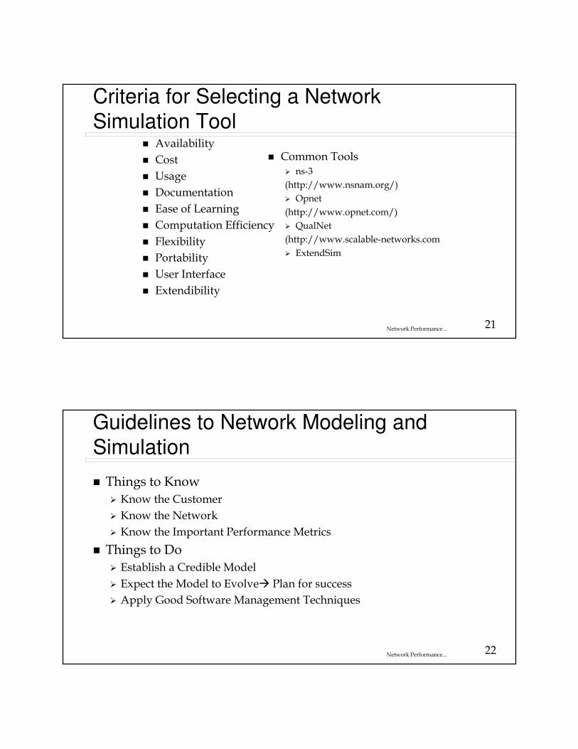
Criteria for Selecting a Network
Simulation Tool� Availability
� Cost
� Usage
� Documentation
� Ease of Learning
� Computation Efficiency
� Flexibility
� Portability
� User Interface
� Extendibility
� Common Tools� ns-3
(http://www.nsnam.org/)
� Opnet
(http://www.opnet.com/)
� QualNet
(http://www.scalable-networks.com
� ExtendSim
22Network Performance...
Guidelines to Network Modeling and
Simulation
� Things to Know
� Know the Customer
� Know the Network
� Know the Important Performance Metrics
� Things to Do
� Establish a Credible Model
� Expect the Model to Evolve� Plan for success
� Apply Good Software Management Techniques
23Network Performance...
Conclusions
� Simulation Can Be an Important Tool for Communication Network Design and Analysis
� Care and Thought Must Go Into Construction of Communication Network Models
� Care and Thought Must Go Into Interpretation of Model Output
24Network Performance...
Extend® Overview
� Allows Graphical Description of Networks� Sources, Links, Nodes, Etc.
� Data Flow Block Diagrams
� Hierarchical Structure to Control Complexity
� Be sure and create libraries when creating complex models

25Network Performance...
Network Performance Evaluation: Elements of
a Queueing System
System
Blockedcustomers
Queue
Server
Server
Server
Departingcustomers
26Network Performance...
Network Performance Evaluation: Elements of
a Queueing System
Servers
Delay
Number in system
Numberin Queue
NumberinServers
27Network Performance...
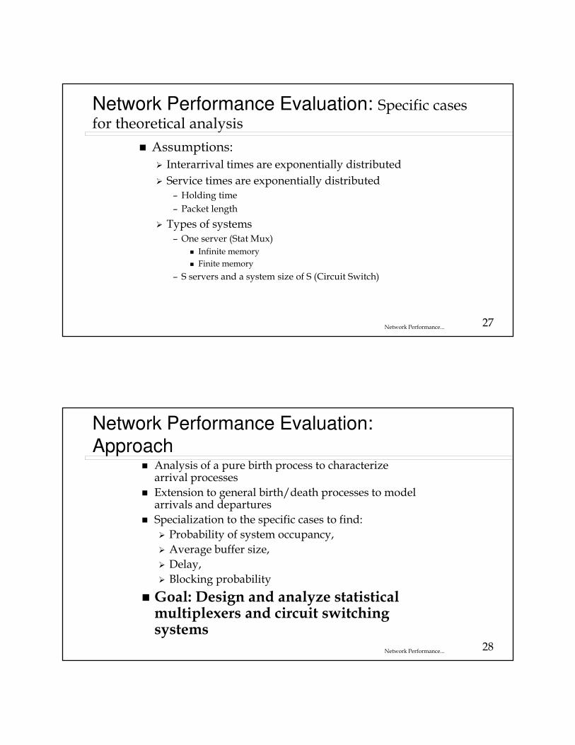
Network Performance Evaluation: Specific cases for theoretical analysis
� Assumptions:
� Interarrival times are exponentially distributed
� Service times are exponentially distributed– Holding time
– Packet length
� Types of systems– One server (Stat Mux)
� Infinite memory
� Finite memory
– S servers and a system size of S (Circuit Switch)
28Network Performance...
Network Performance Evaluation:Approach
� Analysis of a pure birth process to characterize arrival processes
� Extension to general birth/death processes to model arrivals and departures
� Specialization to the specific cases to find:
� Probability of system occupancy,
� Average buffer size,
� Delay,
� Blocking probability
� Goal: Design and analyze statistical multiplexers and circuit switching systems
29Network Performance...
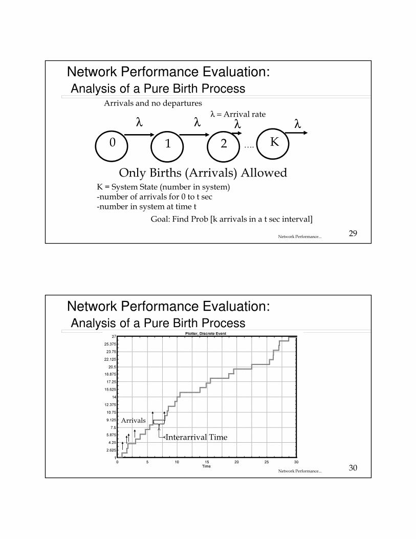
Network Performance Evaluation:Analysis of a Pure Birth Process
Only Births (Arrivals) Allowed
0 1 2 K
λ λλ λ
….
K = System State (number in system)-number of arrivals for 0 to t sec -number in system at time t
λ = Arrival rate
Arrivals and no departures
Goal: Find Prob [k arrivals in a t sec interval]
30Network Performance...
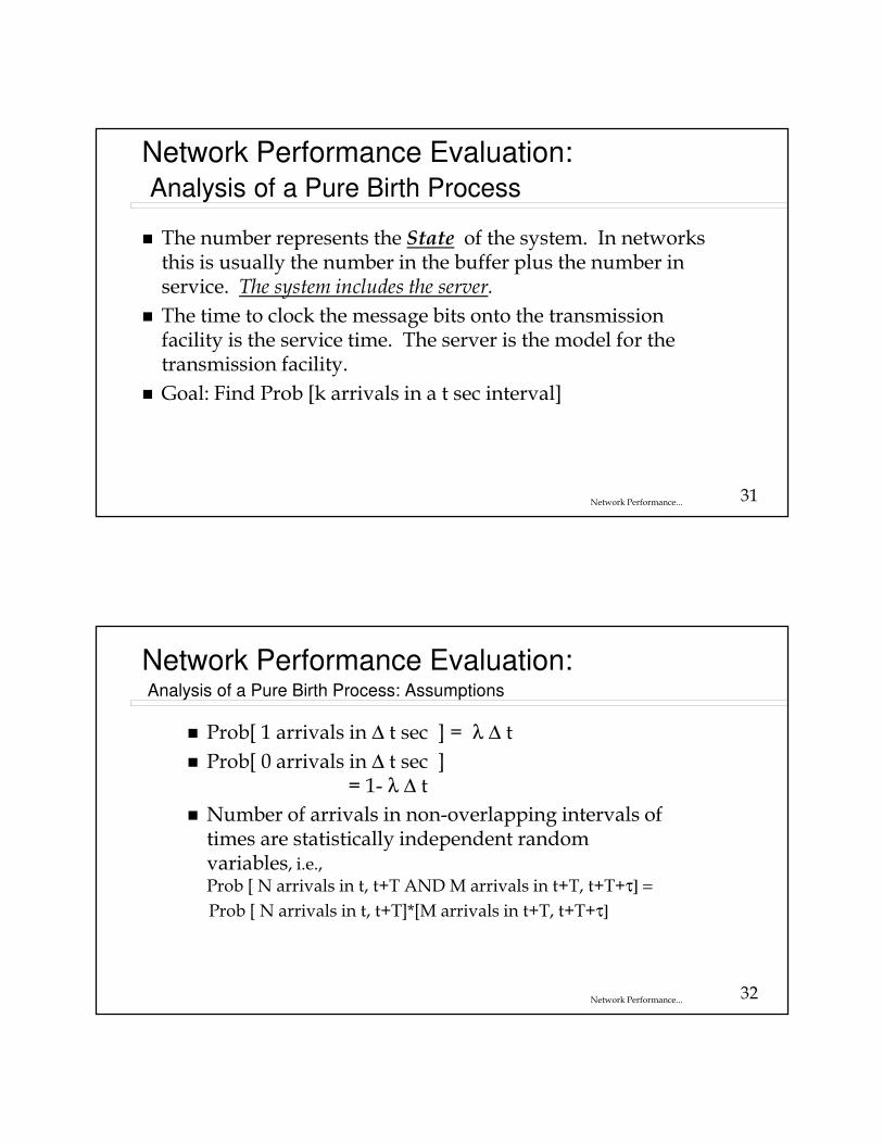
Network Performance Evaluation:Analysis of a Pure Birth Process
Arrivals
Interarrival Time
31Network Performance...
Network Performance Evaluation:Analysis of a Pure Birth Process
� The number represents the State of the system. In networks this is usually the number in the buffer plus the number in service. The system includes the server.
� The time to clock the message bits onto the transmission facility is the service time. The server is the model for the transmission facility.
� Goal: Find Prob [k arrivals in a t sec interval]
32Network Performance...
Network Performance Evaluation:Analysis of a Pure Birth Process: Assumptions
� Prob[ 1 arrivals in ∆ t sec ] = λ ∆ t
� Prob[ 0 arrivals in ∆ t sec ]= 1- λ ∆ t
� Number of arrivals in non-overlapping intervals of times are statistically independent random variables, i.e., Prob [ N arrivals in t, t+T AND M arrivals in t+T, t+T+τ] =
Prob [ N arrivals in t, t+T]*[M arrivals in t+T, t+T+τ]
33Network Performance...
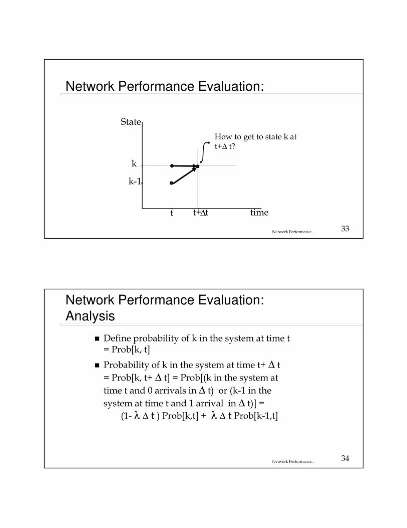
Network Performance Evaluation:
State
k-1
k
t ∆t+ t time
How to get to state k at t+∆ t?
34Network Performance...
Network Performance Evaluation:Analysis
� Define probability of k in the system at time t = Prob[k, t]
� Probability of k in the system at time t+ ∆ t
= Prob[k, t+ ∆ t] = Prob[(k in the system at
time t and 0 arrivals in ∆ t) or (k-1 in the
system at time t and 1 arrival in ∆ t)] =
(1- λ ∆ t ) Prob[k,t] + λ ∆ t Prob[k-1,t]
35Network Performance...
Network Performance Evaluation:Analysis
� Rearranging terms (Prob[k, t+ ∆ t] - Prob[k,t])/ ∆ t + λProb[k,t] = λ Prob[k-1,t]
� Letting ∆ t --> 0 results in the following differential equation:
36Network Performance...
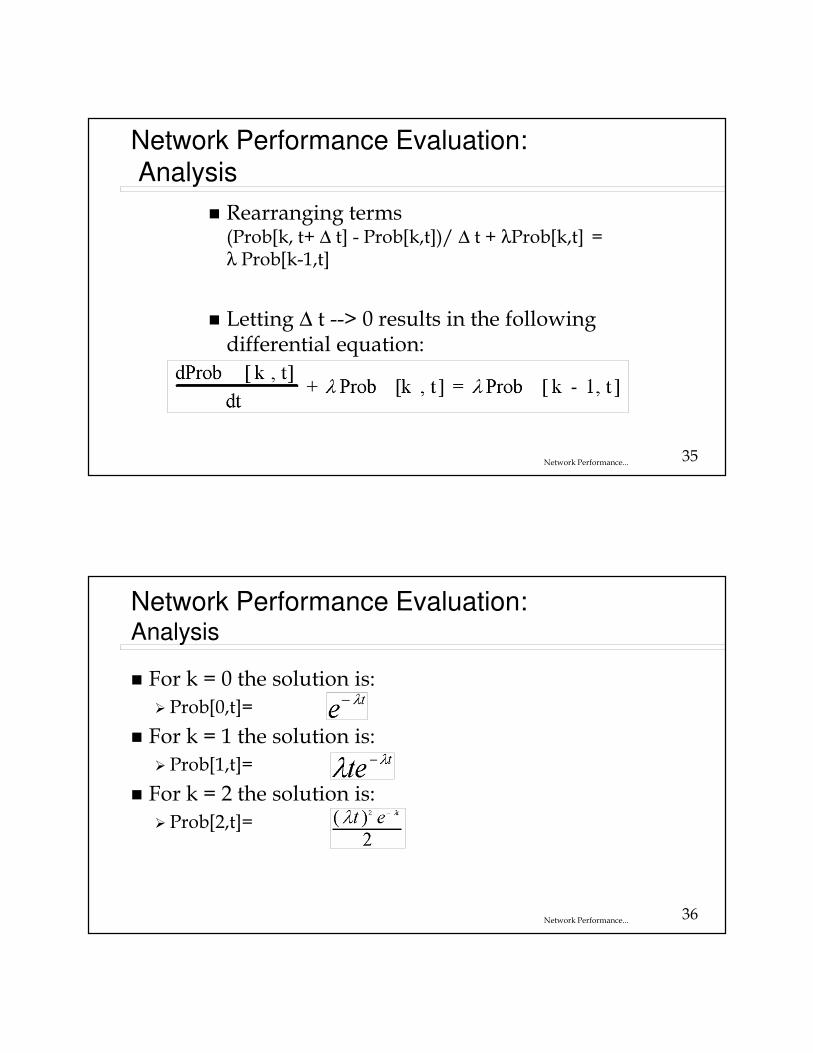
Network Performance Evaluation:Analysis
� For k = 0 the solution is:
� Prob[0,t]=
� For k = 1 the solution is:
� Prob[1,t]=
� For k = 2 the solution is:
� Prob[2,t]=
37Network Performance...
Network Performance Evaluation:Analysis
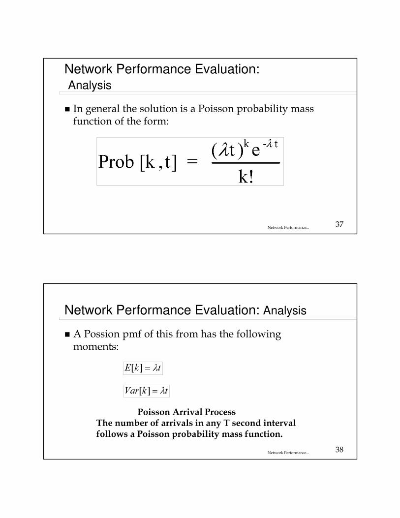
� In general the solution is a Poisson probability mass function of the form:
38Network Performance...
Network Performance Evaluation: Analysis
� A Possion pmf of this from has the following moments:
Poisson Arrival ProcessThe number of arrivals in any T second interval follows a Poisson probability mass function.
39Network Performance...
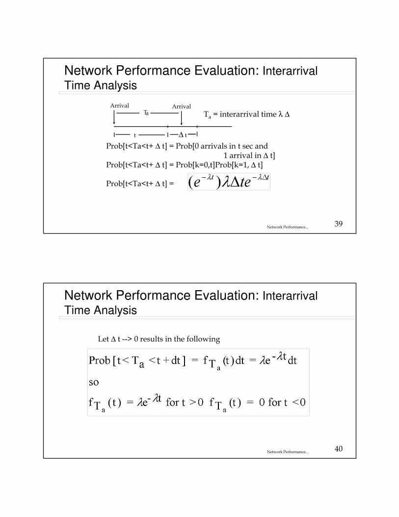
Network Performance Evaluation: Interarrival
Time Analysis
t ∆ t
Arrival ArrivalTa
Prob[t<Ta<t+ ∆ t] = Prob[0 arrivals in t sec and1 arrival in ∆ t]
Prob[t<Ta<t+ ∆ t] = Prob[k=0,t]Prob[k=1, ∆ t]
Prob[t<Ta<t+ ∆ t] =
Ta = interarrival time λ ∆
40Network Performance...
Network Performance Evaluation: Interarrival
Time Analysis
Let ∆ t --> 0 results in the following
41Network Performance...
Network Performance Evaluation:Interarrival Time Analysis
MAIN RESULT:The interarrival time
for a Poisson arrival process followsan exponential probability density function.
42Network Performance...
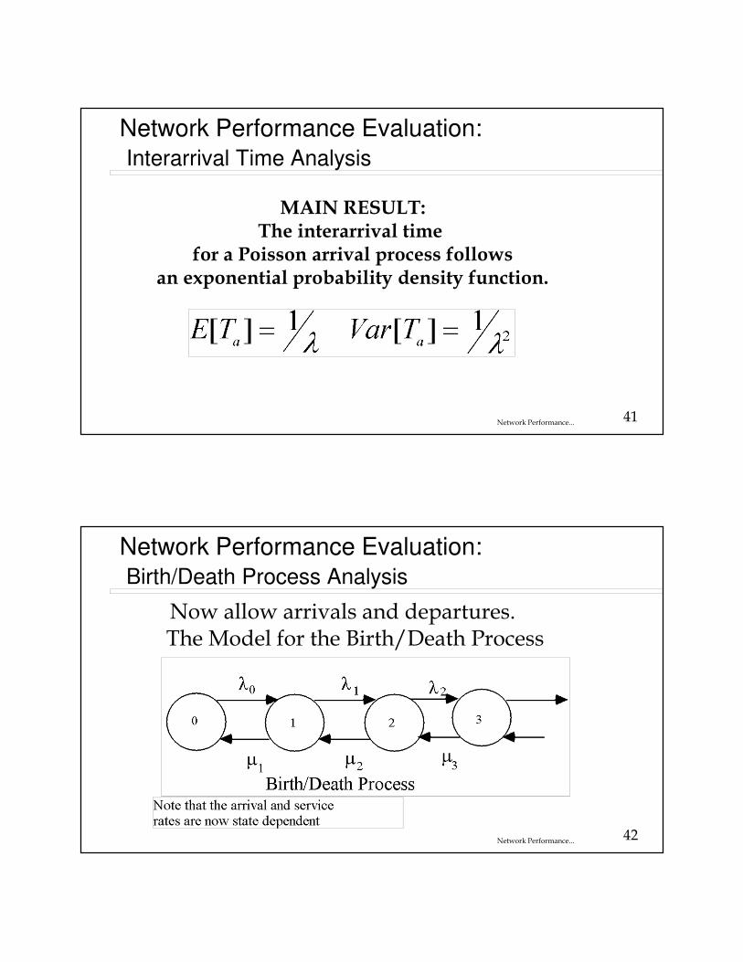
Network Performance Evaluation:Birth/Death Process Analysis
The Model for the Birth/Death ProcessNow allow arrivals and departures.
43Network Performance...
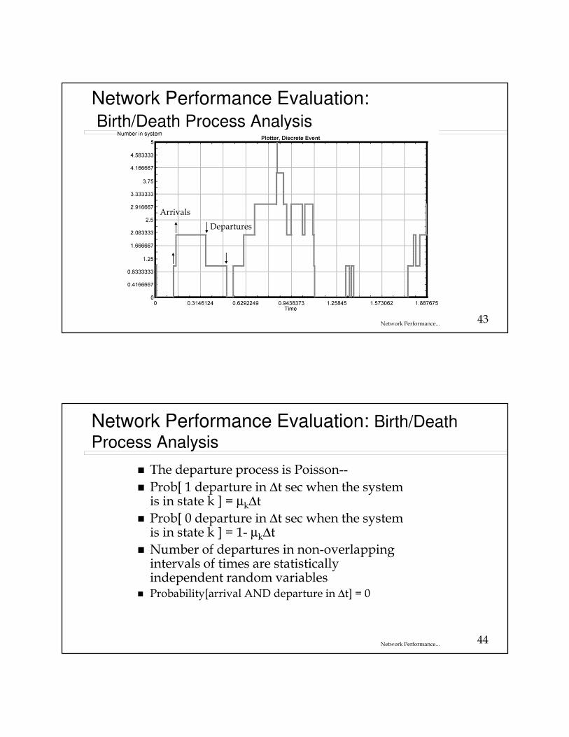
Network Performance Evaluation:Birth/Death Process Analysis
Arrivals
Departures
44Network Performance...
Network Performance Evaluation: Birth/Death
Process Analysis
� The departure process is Poisson--
� Prob[ 1 departure in ∆t sec when the system is in state k ] = µk∆t
� Prob[ 0 departure in ∆t sec when the system is in state k ] = 1- µk∆t
� Number of departures in non-overlapping intervals of times are statistically independent random variables
� Probability[arrival AND departure in ∆t] = 0
45Network Performance...
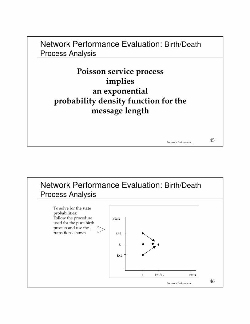
Network Performance Evaluation: Birth/Death
Process Analysis
Poisson service processimplies
an exponential probability density function for the
message length
46Network Performance...
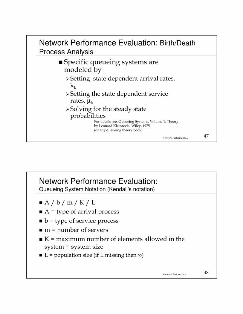
Network Performance Evaluation: Birth/Death
Process Analysis
To solve for the state probabilities:Follow the procedure used for the pure birth process and use the transitions shown
47Network Performance...
Network Performance Evaluation: Birth/Death
Process Analysis
� Specific queueing systems are modeled by �Setting state dependent arrival rates,
λk�Setting the state dependent service rates, µk
�Solving for the steady state probabilities
For details see: Queueing Systems. Volume 1: Theory by Leonard Kleinrock, Wiley, 1975 (or any queueing theory book)
48Network Performance...
Network Performance Evaluation: Queueing System Notation (Kendall's notation)
� A / b / m / K / L
� A = type of arrival process
� b = type of service process
� m = number of servers
� K = maximum number of elements allowed in the system = system size
� L = population size (if L missing then ∞)
49Network Performance...
Network Performance Evaluation: Special
cases: A / b / m / K / L� A= M => the arrival process is Poisson and the interarrival times are independent, identically distributed exponential random variables. (M = Markov)
� b = M => the service process is Poisson and the interdeparture times are independent, identically distributed exponential random variables.
� A or b = G=> times are independent, identically distributed general random variables.
� A or b = D => times are deterministic, i.e., fixed times
� Examples:� M/M/1/∞/∞ (Ideal router output port)
� M/M/1/N /∞ (Real-finite-buffer router output port)
� M/M/S/S /∞ (Circuit Switch)
In Homework will do M/D/1 for VoIP analysis
50Network Performance...
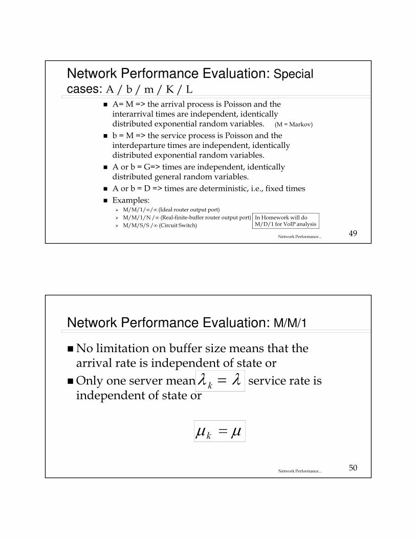
Network Performance Evaluation: M/M/1
�No limitation on buffer size means that the arrival rate is independent of state or
�Only one server means that the service rate is independent of state or
51Network Performance...
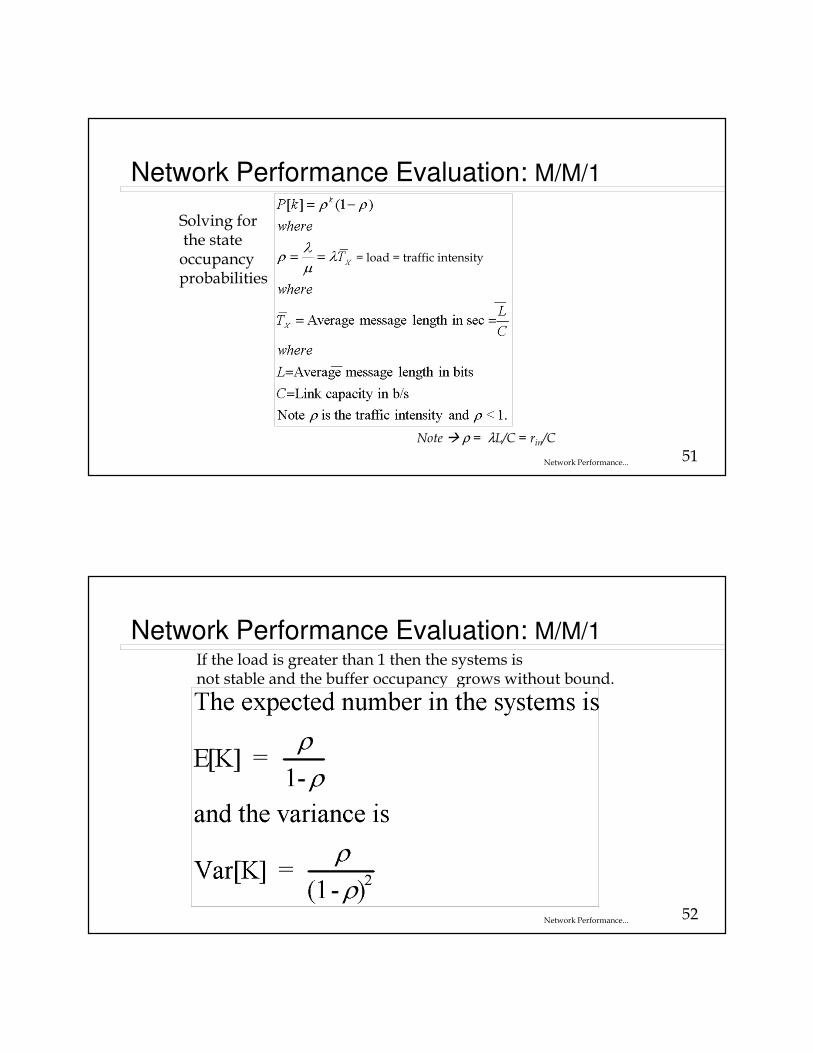
Network Performance Evaluation: M/M/1
Solving forthe state occupancy probabilities
= load = traffic intensity
Note� ρ = λL/C = rin/C
52Network Performance...
Network Performance Evaluation: M/M/1If the load is greater than 1 then the systems is not stable and the buffer occupancy grows without bound.
53Network Performance...
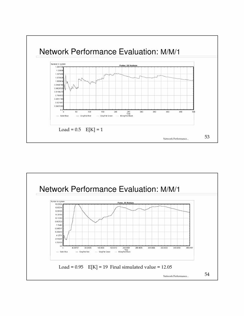
Network Performance Evaluation: M/M/1
Load = 0.5 E[K] = 1
54Network Performance...
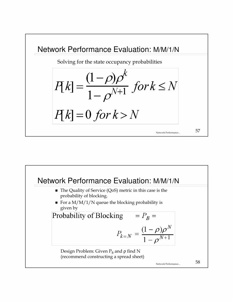
Network Performance Evaluation: M/M/1
Load = 0.95 E[K] = 19 Final simulated value = 12.05

55Network Performance...
Network Performance Evaluation: M/M/1
Load = 0.95 E[K] = 19
56Network Performance...
Network Performance Evaluation: M/M/1/N
� Only one server means that the service rate is independent of state or
� The limitation on system size means that the arrival rate is dependent of state or
57Network Performance...
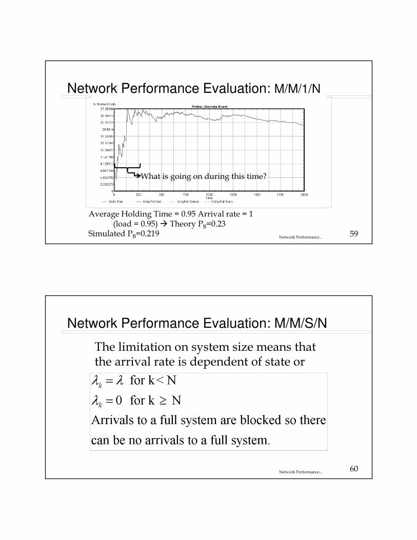
Network Performance Evaluation: M/M/1/N
Solving for the state occupancy probabilities
58Network Performance...
Network Performance Evaluation: M/M/1/N
� The Quality of Service (QoS) metric in this case is the probability of blocking.
� For a M/M/1/N queue the blocking probability is given by
Design Problem: Given PB and ρ find N (recommend constructing a spread sheet)
59Network Performance...
Network Performance Evaluation: M/M/1/N
Average Holding Time = 0.95 Arrival rate = 1 (load = 0.95) � Theory PB=0.23
Simulated PB=0.219
What is going on during this time?
60Network Performance...
Network Performance Evaluation: M/M/S/N
The limitation on system size means that the arrival rate is dependent of state or
61Network Performance...
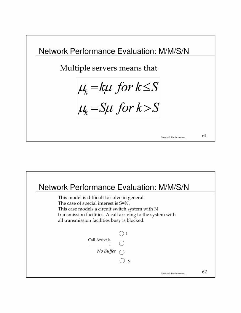
Network Performance Evaluation: M/M/S/N
Multiple servers means that
62Network Performance...
Network Performance Evaluation: M/M/S/NThis model is difficult to solve in general. The case of special interest is S=N. This case models a circuit switch system with N transmission facilities. A call arriving to the system with all transmission facilities busy is blocked.
1
N
Call Arrivals
No Buffer
63Network Performance...
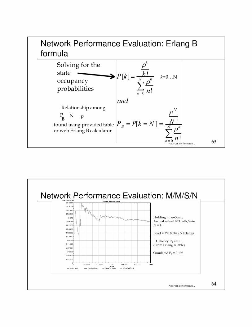
Network Performance Evaluation: Erlang B formula
Solving for the stateoccupancy probabilities
k=0…N
PB
Relationship among
N ρ
found using provided table or web Erlang B calculator
64Network Performance...
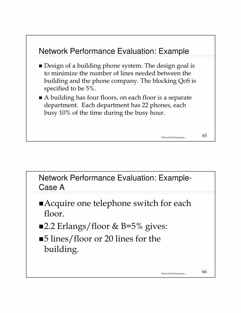
Network Performance Evaluation: M/M/S/N
Holding time=3min, Arrival rate=0.833 calls/minN = 4
Load = 3*0.833= 2.5 Erlangs
� Theory PB = 0.15 (From Erlang B table)
Simulated PB = 0.198
65Network Performance...
Network Performance Evaluation: Example
� Design of a building phone system. The design goal is to minimize the number of lines needed between the building and the phone company. The blocking QoS is specified to be 5%.
� A building has four floors, on each floor is a separate department. Each department has 22 phones, each busy 10% of the time during the busy hour.
66Network Performance...
Network Performance Evaluation: Example-Case A
�Acquire one telephone switch for each floor.
�2.2 Erlangs/floor & B=5% gives:
�5 lines/floor or 20 lines for the building.
67Network Performance...
Network Performance Evaluation: Example-Case B
�Acquire one telephone switch for the building.
� 88 phones @ .1 Erlang/phone = 8.8 Erlangs
� 8.8 Erlangs & B=5% gives:
� 13 lines for the building
� Select Case B
68Network Performance...
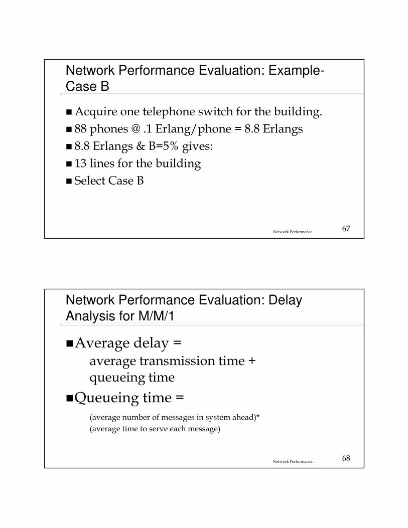
Network Performance Evaluation: Delay Analysis for M/M/1
�Average delay = average transmission time +queueing time
�Queueing time = (average number of messages in system ahead)*
(average time to serve each message)
69Network Performance...
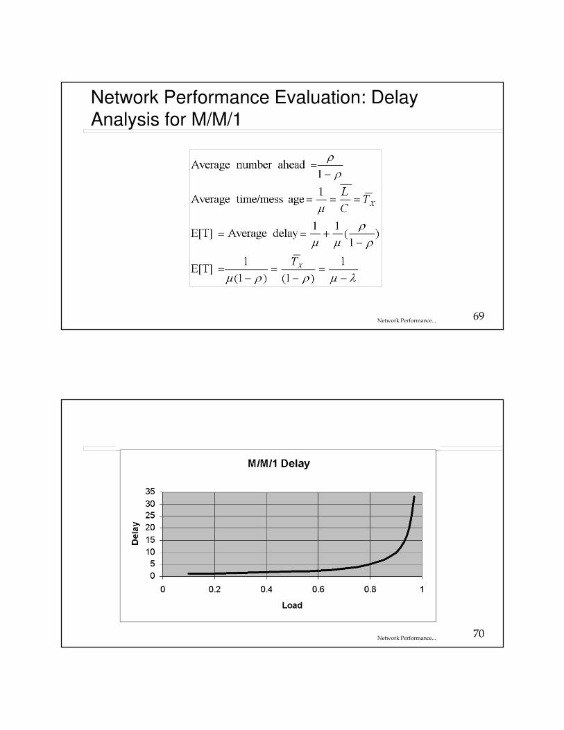
Network Performance Evaluation: Delay Analysis for M/M/1
70Network Performance...
71Network Performance...
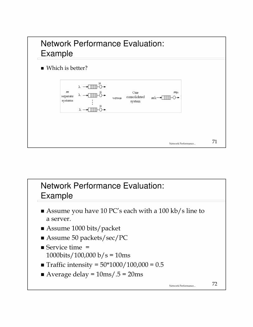
Network Performance Evaluation:Example
� Which is better?
72Network Performance...
Network Performance Evaluation:Example
� Assume you have 10 PC’s each with a 100 kb/s line to a server.
� Assume 1000 bits/packet
� Assume 50 packets/sec/PC
� Service time =1000bits/100,000 b/s = 10ms
� Traffic intensity = 50*1000/100,000 = 0.5
� Average delay = 10ms/.5 = 20ms
73Network Performance...
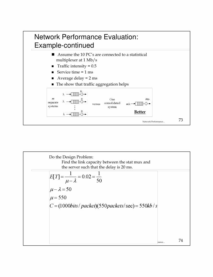
Network Performance Evaluation:Example-continued
� Assume the 10 PC’s are connected to a statistical
multiplexer at 1 Mb/s
� Traffic intensity = 0.5
� Service time = 1 ms
� Average delay = 2 ms
� The show that traffic aggregation helps
Better
74Network Performance...
Do the Design Problem:Find the link capacity between the stat mux and the server such that the delay is 20 ms.
75Network Performance...
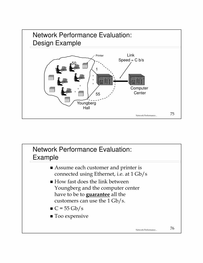
Network Performance Evaluation:Design Example
1
50
YoungbergHall
1
55
Computer Center
Link
Speed = C b/s
Printer
76Network Performance...
Network Performance Evaluation:Example
� Assume each customer and printer is connected using Ethernet, i.e. at 1 Gb/s
� How fast does the link between Youngberg and the computer center have to be to guarantee all the customers can use the 1 Gb/s.
� C = 55 Gb/s
� Too expensive

77Network Performance...
Network Performance Evaluation:Design Example
� Customer performance requirements:
� Delay < 100 ms (use M/M/1 analysis to find C)
� Loss < 10% (use M/ M/ 1/N analysis to find N)
� Assume customer traffic:
� Average packet length = 9000 bytes/packet
� 55 sources
� Packets are generated at a rate of 2 per second/source
78Network Performance...
Network Performance Evaluation:Design Example
� Μ/Μ/1 analysis to find C� λ=55*2 =110 packets/sec
� Ε[Τ] = 100 ms = 1/10 = 1/(µ−λ)
� µ= 120
� C = µ∗L = 120 * 9000 Bytes/packet*8 bits/Byte= 8.64 Mb/s
� M/M/1/K analysis to find system size(K)� Rate_in = (110 packets/sec) * 9000 Bytes/packet*8 bits/Byte = 7.92Mb/s
� ρ= Rate_in/C = (7.92Mb/s)/(8.64 Mb/s) = µ/λ = 110/120 = 0.916
� ρ=0.916 and Blocking Prob = 0.1 � K = 7
� Final design is:
� C = 8.64 Mb/s
� Average system size > 7 packets