Network design for line-based autonomous bus services

Jonas Hatzenbuhler1,∗, Oded Cats1,2, Erik Jenelius1

KTH Royal Institute of Technology, 100 44 Stockholm, Sweden

Abstract

The maturing of autonomous driving technology in recent years has led to several pilot projects and the initial in-tegration of autonomous pods and buses into the public transport (PT) system. An emerging field of interest is thedesign of public transport networks operating autonomous buses and the potential to attract higher levels of traveldemand. In this work a multi-objective optimization and multi-agent simulation framework is developed to study po-tential changes in the network design and frequency settings compared to conventional PT systems when autonomousvehicles (AV) systems are deployed on fixed-route networks. During the optimization process multiple deploymentscenarios (network configurations and service frequency) are evaluated and optimized considering the operator cost,user cost and infrastructure preparation costs of the system. User-focused network design and operator-focused net-work design are studied for a real-world urban area in Sweden. The results provide insights into the network designand level of service implications brought about by the deployment of autonomous bus (AB) when those are integratedin route-based PT systems. We show that the deployment of autonomous buses result with a network design thatincreases service ridership. In the context of our case study this increase is likely to primarily substitute walking.

Highlights:

• simulation-based multi-objective optimization of transit network design and frequency setting prob-lem

• the case study showed that a deployment of autonomous buses can lead to a doubling of passengerload

• reduction of operator cost through autonomous buses leads to an improved level of service for user-focused PT networks

Keywords: Public transport, Automated Bus, Network Design, Simulation-based multi-objective Optimization

1. Introduction

The current technological advances in the field of autonomous buses (AB) allow for tests and operations of ABon public roads. These pilot studies target investigations of user acceptance and vehicle operation of AB in transportsystems. Most pilot studies either offer last-mile connections from a transportation hub or close a transportation gapbetween two stations. When operating AB as a transport mode on fixed routes the operating costs are expected to5

reduce by ca. 50% compared to conventional bus operations (Lidestam et al., 2018). Walters (1982) showed that anoperating cost reduction facilitates a shift in resource allocation towards higher service frequencies and lower vehiclecapacities. With higher frequencies and smaller vehicles changes in the route network layout are possible. Eluru

∗Corresponding author:Email address: jonashat@kth.se (Jonas Hatzenbuhler)

1Division of Transportation Planning, KTH Stockholm, Sweden2Department of Transport and Planning, Delft University of Technology, Netherlands

Preprint submitted to Transportation Received: March 17, 2020

and Choudhury (2019) present eight different studies discussing potential impacts of autonomous vehicles on tripgeneration, vehicle-miles traveled and other transport related metrics. All these studies assume demand-responsive10

autonomous vehicles no line-based operations. In contrast to these studies, we elaborate more holistically on theimpacts of autonomous vehicles on the combined operator, infrastructure and user costs on fixed-line services, whichdeepens the understanding of system level impacts due to AB deployment. Additionally we can get insights in howthe reduction of operator costs in case of AB deployment effects the level of service for public transport users.

15

The transit network design and frequency setting problem (TNDFSP) is characterized as creating an optimal set ofpublic transport bus routes including the service frequency for each bus route operating in the network. The problemhas been subject to extensive research in the last decades. However, even though vehicle automation has the potentialto greatly impact service design properties, it has not yet been systematically investigated. In this work, we formulatea variant of the TNDFSP that caters for the characteristics of AB and hence allows examining the potential impacts of20

its deployment on service design. With the deployment of AB additional constraints regarding the connectivity of thebus lines are required. More specifically every bus stop should be connected in the network with every other bus, sothat all bus stops can be reached by any bus. This property has not been considered in past TNDFSP formulations. Theline-based network characteristics and the connectivity constraint are motivated twofold. First, the use of a line-basedpublic transport system is known to most people and has been accepted for a long time and has important merits in25

serving the bulk of the travel demand. Second, the legal operation of autonomous buses in most urban environmentsis currently bound to certain areas and or specific roads. The legislative framework does not allow for the deploymentof large fleet sizes in flexible operational environments; hence the line-based mode of operation is seen as the firstpractical use case. By adding line-based and connectivity characteristics to the problem formulation the study inves-tigates near future and transition scenarios from traditional to autonomous public transport operations. Additionally,30

the deployment of AB affects the operational cost structure by reducing the crew cost as well as the infrastructure costby increased costs for AB specific road or bus stop enhancements. The impact of both cost terms on the TNDFSP hasnot been studied previously. Further, the majority of past research on TNDFSP requires PT networks to serve everybus stop. In this AB specific TNDFSP the bus stop position is an output value. Thus, not every potential bus stop inthe area of interest has to be served. This allows for a network design which is simultaneously benefiting operator35

focused designs and serving the demand with a user perspective in mind.

In this study, we investigate how the network design (number of routes and route alignment), the infrastructure(number of bus stops and network length), operating and traveler costs are affected by changed supply characteristics(service frequency and vehicle capacity) induced by AB. Additionally, the study investigates the impact of changes in40

supply provision on user costs and consequently its potential impacts on ridership. Furthermore, structural differencesin user-focused network design and operator-focused network design are investigated. We solve the TNDFSP usinga simulation-based multi-objective optimization framework. The created solutions are constrained by the maximumnumber of routes, the maximum service frequency and number of bus stops per route. The use of a agent-based simu-lation module allows the simulation of walking as a transportation mode. By this passengers have the option to board45

a bus or walk at every bus stop and at every point in time. This is achieved by additional walking links added to thenetwork design problem.

The remaining of the paper is structured as follows. First, the relevant literature is reviewed in section 2. Thenthe methodology of this study is described in section 3. In section 4 the case study is detailed. The following sec-50

tion 5 discusses the impact of AB on the network design, differences between user-focused and operator-focused PTnetworks and benchmark results. The remaining of the paper (Section 6) critically assesses the results and concludesabout the applicability of the framework. This section closes with an outlook, sketching directions for potential futurestudies.

55

2. Literature Review

This section reviews the relevant literature. First, works one transit network design and frequency setting problemsare presented and second studies presenting passenger assignment models in PT are introduced.

2

2.1. Network design60

The strategic public transport planning process can be subdivided into five consecutive steps (Ceder and Wilson,1986). Step one is network design where demand and supply data are used to create routes and operation strategies.In the second step, the service frequencies are determined based on the available vehicle fleet, policy constraints, andthe created routes. In the next step, the timetable is developed which results in trip arrival and departure times foreach stop in the network. The fourth step is solving the vehicle scheduling problem based on schedule constraints,65

deadheading and work hour times. In the last step, the crew schedule is created. In the past, studies have proposedsolutions for each of the five steps. Recent developments include the combined solution of multiple steps (see e.g.Michaelis and Schobel (2009)). Guihaire and Hao (2008) provide an extensive literature study about research ontransit network design and scheduling. They categories the original five-step approach by grouping (a) the first andsecond steps, (b) the second and third steps and (c) all first three steps together. The resulting problem categories70

are (a) transit network design and frequency setting problem (TNDFSP), (b) transit network frequency setting andscheduling problem (TNSP) and (c) transit network design and scheduling problem (TNDSP), respectively. In thisstudy, we focus on the first combination, the TNDFSP. The solution for this problem implies finding a set of routes toserve a given area and their respective frequencies.

75

Transit design and transit planning problems are challenging to solve (Guihaire and Hao, 2008). In Magnanti andWong (1984) the authors state multiple transit network design problem formulations and elaborate on their complexity.The authors conclude that the general network design problem is NP-hard and therefore requires certain heuristics tobe solved for large problem instances. Similarly, sub-problems of the general network design have been proven to beNP-hard, e.g. the uncapacitated budget design Johnson et al. (1978), the Steiner tree on a graph Garey and Johnson80

(1979).Table 1 provides an overview of selected studies that developed and applied heuristics or meta-heuristics to solve

the TNDFSP. For each study, we mention the elements included in the objective function, decision variables and con-straints; the solution method and the demand-related assumptions.

85

Table 1: Literature Overview TNDFSP

Author Objective Decision Variables Constraints Method Demand pattern Demand

Lampkin and d. Saalmans (1967) Number of direct passengers, total travel time Fleet size Routes, frequencies Heuristic Many to many InelasticMandl (1980) Routes directness, travel time Routes Constant frequency, service coverage Heuristic Many to many InelasticBaaj and Mahmassani (1991) Total travel time, number of buses Routes, frequencies Frequencies, load factor, fleet size Heuristic Many to many InelasticCeder and Israeli (1998) Operator and user costs, fleet size Routes, frequencies Route length, deviation from shortest path Heuristic Many to many InelasticChien et al. (2001) Total welfare Routes, headways Capacity, budget Heuristic GA Many to one Differs within zones

(user and operator cost)Chakroborty and Wivedi (2002) In-vehicle time, unsatisfied demand, number of Routes Road network Heuristic GA Many to many Inelastic

direct, 1-transfer, 2-transfer passengerstransfers, number of buses

Chien et al. (2003) Total welfare Routes, headways Passenger load Heuristic Many to one Service dependent(user and operator cost)

Chakroborty (2003) Sum of transfers Binary variable, Routes, vehicle capacity, Heuristic GA Many to one Inelasticand waiting time transfer count maximum waiting time

Fan and Machemehl (2006) Sum of travel time incl. transfer time, Number of routes, Routes, capacity, fleet size Heuristic SA Many to one Inelasticoperation costs and unsatisfied demand travel time between nodes

Zhao and Zeng (2008) Service coverage, Routes, frequencies Route directness Heuristic Many to many InelasticMinimization of transfers SA/tabu search

Szeto and Jiang (2012) Travel time and Binary values for node connectivity and Route topology, capacity, fleet size, Heuristic ABC Many to many Inelasticunsatisfied demand route start/end, service frequency transfers

Szeto and Jiang (2014) Upper level: transfers Binary values for node connectivity and Route topology, capacity, fleet size, Bi-level Heuristic ABC Many to many InelasticLower level: vehicle load and waiting time route start/end, service frequency transfers

Possel et al. (2018) Sum of Emissions, accident fatalities Traffic flow, travel time Not stated Heuristic GA and SA Many to many Service Dependentand travel time

Bourbonnais et al. (2019) Sum of travel time, Not stated Not stated Heuristic GA Many to many Inelasticunsatisfied demand and vehicle hours

Proposed Approach User Cost, Operator Cost, Infrastructure Cost Routes, frequencies Route length, cyclic service frequency, connectivity, capacity ABC and Simulation Many to many Inelastic

In most studies heuristic algorithms are employed to solve large scale network design problems. The heuristicapproaches include simulated annealing (SA), tabu search, genetic algorithm (GA) and artificial bee colony optimiza-tion (ABC) as well as other more niche algorithms for specific problems. Most of the variation in the studies lies inthe details of the problem formulation and the size of the investigated network. In Lampkin and d. Saalmans (1967)the authors simultaneously optimize vehicle capacity and travel time of a single route network. The demand level is90

fixed and many-to-many origin-destination demand scenarios are assumed. The approach optimizes a social welfareobjective function characterizing the user cost and operator cost as a monetary value. More sophisticated models

3

(Zhao and Zeng, 2008; Chien et al., 2003; Chakroborty, 2003) apply several constraints regarding the travel experi-ence in the network. Hence the number of transfers, the directness of the routes and the number of stops on eachroute are controlled by appropriate constraint formulations. Fan and Machemehl (2006) present a simulated anneal-95

ing algorithm to solve the TNDFSP. The algorithm objective is the combined cost of user, operator and unsatisfieddemand. The problem is constrained by the maximum route capacity, maximum fleet size, maximum trip length andmaximum number of routes. The authors apply the framework to a test network consisting of 160 nodes and 418edges. They conclude that the results based on SA are converging to lower total cost values compared to applying GAto this problem. Similarly, Bourbonnais et al. (2019) utilize a GA algorithm to solve TNSFP using road network data.100

They optimize the sum of satisfied transit demand, unsatisfied transit demand and vehicle-hours. The authors showthe applicability of their framework on three cities in Quebec, Canada.

A multi-objective network design formulation is proposed by Possel et al. (2018). The objectives are based on totalemissions, the number of traffic accident fatalities and the total travel time. The main contribution is the formulation105

of a bi-level program which has the minimization of the objectives on the upper level and the passenger assignmenton the lower level. The authors compare the optimization algorithm NSGA-II with simulated annealing algorithmsand show the minor dominance of the NSGA-II. Szeto and Jiang (2012) discuss the application of an ABC algorithmfor the TNDPFSP. The objective value is computed as the weighted sum of passenger transfers and travel time. Theproblem is constrained by the vehicle fleet size. The service frequency is determined by a heuristic considering the110

maximum available vehicles per route. In a later work Szeto and Jiang (2014) design a bi-level optimization approachfor the network design problem utilizing a linear program for the frequency assignment as the bottom-level problemand an ABC approach for the top-level route creation problem. The authors apply their framework to a small syntheticnetwork as well as the entire public transport network of Winnipeg, Canada and Tin Shui Wai, China. It is concludedthat the ABC algorithm outperforms genetic algorithm for large networks.115

To evaluate the user cost for a given network design passengers must be assigned to service routes. Existingpassenger assignment models can be classified into static and dynamic models, with deterministic or stochastic andfrequency-based assignment (Nguyen and Pallottino, 1988; Spiess and Florian, 1989; Cepeda et al., 2006) or schedule-based assignment (Mark D. Hickman and David H. Bernstein, 1997; Tong and Wong, 1998; Poon et al., 2004). Liu120

et al. (2010) give a comprehensive overview of past and ongoing research in transit assignment models. With staticassignment models the demand and supply are assumed to be constant over the period of analysis, hence within-daychanges, e.g. variations in vehicle crowding and waiting times, cannot be studied (Liu et al., 2010). Additional tothe analytical approaches for the network design problem, studies integrating simulation models into the optimizationframework have recently been published. Neumann (2014) proposes a framework consisting of the agent-based125

simulation software MATSim and a genetic algorithm to design public transport networks for paratransit vehicleoperations. The network is defined as a set of routes each serving a sequence of stops and each having a dedicated starttime. The genetic algorithm adjusts the route layout and operation starting times. The simulation model then computespassengertrip plans and movements throughout the network. The study replicates reference network operations andimprove the operations in non-profitable public transport corridors. The main limiting factor of the framework, as130

stated by the authors, is the limited search space.

2.2. Scientific ContributionIn a related study by Kim et al. (2019) the authors use a simulation based approach to evaluate what impact au-

tonomous buses have on the departure times for commuting trips. In their study the authors did not assume a publictransport network but rather taxi-like operations using AB rather than private vehicles. The authors could show that,135

in the autonomous case for many commuters the desired and actual departure time are not the same. The authorsconclude that the additional policy regulations (e.g. dynamic pricing schemes or travel reservations) must be imple-mented to make autonomous taxi operations more popular.

The main contribution of this work is an AB specific network design and frequency setting problem, which aims140

to realistically represent passenger decisions and transport supply. For the analysis of AB systems, it is important tohave a realistic and detailed passenger assignment with which it is possible to identify bottlenecks in passenger flow.Therefore, a dynamic passenger assignment model with with-in day characteristics is chosen in this study. Through

4

the addition of walking links on the entire network the design public transport network a realistic competing mode forthe bus lines is implemented. The characteristics of autonomous buses compared to conventional buses are captured145

by presenting an adjusted operator cost model. Autonomous bus specific infrastructure costs for dedicated lanes andautonomous bus specific bus stops are assumed. The network design is also constrained to create connected PT net-works in which every AB can reach every bus stop in the network without human interaction. In contrast to recentwork in network design we formulate the problem as a multi-objective optimization problem to optimize simultane-ously for user cost, operator cost and infrastructure costs.150

In comparison to Neumann (2014) the proposed framework in this work differs in two ways. First, the user cost isincorporated as an additional objective function component rather as an additional objective, which means that userand operator interests are directly competing with each other. Second, the implemented heuristic optimization algo-rithm allows for a more efficient optimization of large solution spaces compared to a genetic algorithm, which allows155

for larger scenarios and more robust solutions.

5

3. Methodology

This section describes the proposed formulation and solution approach for the multi-objective transit network de-sign and frequency setting problem (TNDSFP) with autonomous buses. First, the problem formulation is introduced.160

Then an overview over the different objectives is given. The section closes with the description of the solution ap-proach employed.

3.1. Problem formulationWith the proposed problem formulation the impact of AB on the network design for the users, operators and165

authorities of PT systems can be computed. The problem is formulated as a multi-objective problem where eachobjective represents one stakeholder. The detailed formulation is given in the following subsections. To rate differentsolutions and analyze the impact of AB the network design is assessed using key performance indicators (KPI), suchas walking times, in-vehicle times, number of transfers, passenger load, number of bus stops and cycle times of vehi-cles.170

The decision variables of the problem are; (1) number of bus routes, (2) the frequency of each route and (3) thebus stops served by each route. The design of the network is constrained by the maximum number of routes, and theminimum and maximum number of bus stops per route. To cater for AB specific requirements, the network of busroutes has to be connected so that each vehicle can reach any bus stop (connected graph) and that one bus stop is175

not served twice on the same route (non-cyclic route). This connectivity constraint is motivated by the assumed ABoperations. If a bus is driven autonomously there should always be the possibility to autonomously drive back to thedepot without any human interaction. Additionally, it should be possible for every bus to reach every position in thenetwork so that in case of technical failures other buses could compensate. The infrastructure cost incorporates thefact that AB operations require e.g. dedicated lane operations and technology enhanced bus stops. The number of bus180

stops is an output of the framework. The input values are the road network graph, set of potential bus stops and anOD matrix.

3.1.1. Network definitionWe consider a two-layer network representation to capture the infrastructure constraints and costs associated with185

the deployment of AB in addition to the service configuration. The bottom-level graph represents the physical roadnetwork (infrastructure graph). The nodes in this graph represent the road start- and endpoints and intersections. Anedge in the graph is a road section on which an AB can operate. The top-level graph represents the bus stop connec-tivity (service graph). A node in this graph is a bus stop or bus hub. A bus stop is served by one service route, whereasa bus hub is served by a minimum of two service routes. An edge in the top-level graph is the shortest path connecting190

two bus stops, based on the bottom level graph connecting of these two nodes. We add the number and position of allpotential bus stops in the network are provided as input. A service route is defined as a sorted list of bus stops in thesecond level graph. Figure 1 shows the relation between the two graphs.

Besides the bus routes also walking links are added to the network. Passengers have the option to walk between195

every pair of nodes if these nodes are not more than 300m apart. For rapid transit operations a bus stop distance ofminimal 500m is required by the latest report of the City of Stockholm (see Firth (2012)). Based on the geographicalsize of the studied network and the operation speed of the buses 300m as the threshold distance are assumed reason-able since only a few bus stops are further apart, hence passenger have the option to reach nearly every point in thenetwork by foot.200

3.1.2. Demand formulationThe demand is represented as an origin-destination matrix with a distinct time-dependent passenger arrival rate

(pax/h) for each origin-destination pair. The origin and destination are defined as bus stops in the network. Thedemand matrix is a required input to the model. A path is the route or combination of routes a passenger chooses205

6

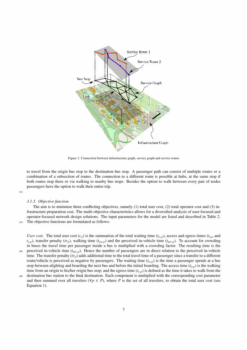
Figure 1: Connection between infrastructure graph, service graph and service routes

to travel from the origin bus stop to the destination bus stop. A passenger path can consist of multiple routes or acombination of a subsection of routes. The connection to a different route is possible at hubs, at the same stop ifboth routes stop there or via walking to nearby bus stops. Besides the option to walk between every pair of nodespassengers have the option to walk their entire trip.

210

3.1.3. Objective functionThe aim is to minimize three conflicting objectives, namely (1) total user cost, (2) total operator cost and (3) in-

frastructure preparation cost. The multi-objective characteristics allows for a diversified analysis of user-focused andoperator-focused network design solutions. The input parameters for the model are listed and described in Table 2.The objective functions are formulated as follows:215

User cost. The total user cost (cu) is the summation of the total waiting time (tw,p), access and egress times (ta,p andte,p), transfer penalty (trp), walking time (twa,p) and the perceived in-vehicle time (tpiv,p). To account for crowdingin buses the travel time per passenger inside a bus is multiplied with a crowding factor. The resulting time is theperceived in-vehicle time (tpiv,p). Hence the number of passengers are in direct relation to the perceived in-vehicle220

time. The transfer penalty (trp) adds additional time to the total travel time of a passenger since a transfer to a differentroute/vehicle is perceived as negative by passengers. The waiting time (tw,p) is the time a passenger spends at a busstop between alighting and boarding the next bus and before the initial boarding. The access time (ta,p) is the walkingtime from an origin to his/her origin bus stop; and the egress time (te,p) is defined as the time it takes to walk from thedestination bus station to the final destination. Each component is multiplied with the corresponding cost parameter225

and then summed over all travelers (∀p ∈ P), where P is the set of all travelers, to obtain the total user cost (seeEquation 1).

7

Table 2: Input parameter for network design framework

Parameter Description Unit

Objective Functionγ

operf ixed unit fixed operating cost SEK/(h-veh)

γcptlf ixed unit fixed capital cost SEK/(h-veh)γ

operunit unit size-dependent operating cost SEK/(h-pax-veh)γ

cptlunit unit size-dependent capital cost SEK/(h-pax-veh)κ vehicle capacity pax/vehη reduced fixed unit operating cost -β additional fixed unit capital cost -δ additional fixed bus stop cost -ε additional fixed road infrastructure cost -

γstop fixed building costs for one bus stop SEK/stopγlink fixed building costs for 1000-pax-km road SEK/(1000-pax-km)υ value of time for public transport users SEK/h

γwt waiting time cost -γwa walking time cost -γivt in-vehicle time cost -γatet access and egress time cost -γtr transfer cost -

Optimizationλ number of bees -Ψ number of iterations -τ number of trails -

cu =

γwa ·∑p∈P

twa,p + γwt ·∑p∈P

tw,p + γivt ·∑p∈P

tpiv,p + γatet ·∑p∈P

(ta,p + te,p) + γtr ·∑p∈P

tri

· υ (1)

If a bus stop is not served by any route in the solution network or if walking gives a higher utility than taking PT,passengers can walk to the closest served bus stop or walk to their final destination. Unsatisfied demand is accounted230

for through the walking time incurred when passengers decide the walk their entire trip.

Operator cost. The operator cost (co) is the summation of capital costs (ccptl) and operating costs (coper) for the ve-hicle fleet. The minimum required fleet size (nr) can be estimated using the frequency ( fr) and cycle time (tr) of abus route (r) (nr = tr · fr/60). The AB specific operating cost and capital costs formulations are in accordance to the235

formulations in Zhang et al. (2019).

The operating cost (coper) is the cost per hour considering the driver and the maintenance costs. In Equation 2the formula for conventional buses and AB is shown. The fleet size per route is multiplied by the summation of theunit fixed and unit size-dependent operating cost parameter. The vehicle capacity is denoted with κ. For AB the unit240

fixed operating cost parameter is reduced by η and for conventional bus operations this parameter is set to zero. Theoperator cost for the network is achieved by the summation of all routes.

coper =∑r∈R

tr · fr60

((1 − η)γoper

f ixed + γoperunit · κ

)(2)

The capital cost (ccptl) is defined as the fixed price for a vehicle depending on capacity and vehicle type. In Equa-tion 3 the formulation for the total capital cost of conventional buses and AB is shown. The capital cost for one routeis the multiplication of fleet size and the unit fixed/size-dependent capital costs (γ), which is summed over all routes245

8

to arrive at the total capital cost. For autonomously operated routes an additional fixed unit capital cost (β) factor isadded and for conventional bus operations this parameter is set to zero.

ccptl =∑r∈R

tr · fr60

((1 + β)γcptl

f ixed + γcptlunit · κ

)(3)

Infrastructure cost. The infrastructure cost (cin f ra) considers the building cost of a bus stop and the total length of thenetwork. The building cost of one bus stop (γstop) is the fixed cost of building all stops serviced by at least one bus line.250

The parameter δ represents additional bus stops costs for AB operations, through e.g. larger bus stops and additionalfences. In conventional bus scenarios δ = 0 holds. The cost associated with the length of the network is computedas the total network length (

∑r∈R lr), where lr is the length of bus route r ∈ R, multiplied with the road infrastructure

building costs (γlink). This additional cost proportion ε considers AB specific infrastructure preparations, e.g. roadmarkings and dedicated lanes. In conventional bus operations ε = 0. In Equation 4 sr is the number of bus stops255

served per route by the network solution.

cin f ra =∑r∈R

((1 + δ) γstop · sr + γlink · lr · ε

)(4)

3.1.4. Mathematical problem formulationThe multi-objective optimization problem is formulated as follows:

minF,R

Q1 = cu(F,R), (5)

minF,R

Q2 =∑r∈R

tr · fr60

[((1 + β)γcptl

f ixed + γcptlunit · κ

)+

((1 − η)γoper

f ixed + γoperunit · κ

)], (6)

minR

Q3 =∑r∈R

((1 + δ) γstop · sr + γlink · lr · ε

), (7)

subject to f min ≤ fr ≤ f max ∀r ∈ R (min./max. service frequency), (8)smin ≤ sr ≤ smax ∀r ∈ R (min./max. stops per route), (9)

rmin ≤ |R| ≤ rmax (min./max. number of routes) (10)

where F = f1, ..., f|R| is the set of all line frequencies. R is the set of routes, sr is the number of bus stops on route260

r and fr is the service frequency. The input value of potential bus stops chosen to be large and evenly distributed overthe area of interest. The first objective is representing the user cost, which is calculated based on output extractedfrom the simulation model. In the simulation module further operational constraints (e.g. vehicle capacity, pick-upand drop-off timing of passengers, bus stop order along a route) are considered.

265

3.2. Solution approach

The TNDFSP is a combinatorial optimization problem. The complexity of the network design problem growsexponentially with the input dimensions. In (Magnanti and Wong, 1984; Farahani et al., 2013) the authors showthat the network design problem is NP-hard. Similar problems such as the widely studied vehicle routing problem(Lenstra and Kan, 1981; Toth and Vigo, 2002), transport line design (Bussieck, 1998) and frequency setting problem270

(Michaelis and Schobel, 2009), have the same characteristics and have been proven to be NP-hard, therefore withthe exception of very small instances, model applications need to be solved using heuristic optimization algorithms.The optimization algorithm for the TNDFSP used in this study is a variant of the multi-objective artificial bee colony(MOABC) heuristic optimization algorithm as described in Szeto and Jiang (2014); Zou et al. (2011) and the NSGA-II algorithm which was first proposed by Deb et al. (2002). This variant allows for the solution of multi-objective275

9

problems and includes AB specific characteristics. In Figure 2 the overall methodology of this study is presented.The optimization problem is framed with the light grey box. The input to the optimization layer is the initial solu-tion set and the two-level graph, which contains the mapping information of all bus stops onto the underlying roadnetwork. The output of the MOABC is a network design solution including the sequence of bus stops on each route,frequency settings for each route and the corresponding objective values. The frequency setting is computed in three280

steps (compare 2). First, the solution is simulated using high service frequencies and high vehicle capacities for eachroute. After the passenger assignment on this solutions the passenger load of each route is determined. Third, theservice frequency for each route is then determined by computing using the determined passenger load per route andthe vehicle capacity of that route. With the assigned service frequency the PT network is simulated and the cost termscomputed based on the simulation outputs. Trails represent the number of network evaluations in the neighborhood285

of a given solution. If the maximal number of trails is not met the same PT network is used as the basis for the nextiteration. Once the termination criteria is met the best PT network solutions are stored. If the termination criteria(maximum number of iterations or hypervolume convergence) are not met and the maximum number of trails is met,the route with the lowest passenger load is removed from the network (Figure 2). The hypervolume for a solution isthe volume of a cuboid which has its two diagonal points as the reference point and the solution vector, respectively.290

The reference point was chosen to be the origin and the solution vector is a 3-dimensional vector where each objectivevalue is one dimension.

3.2.1. InputThe framework requires three different input data sets: the demand as an OD matrix, the potential bus stop posi-295

tions, and the road network. The road network is needed to compute the distances between bus stops and representsthe feasible operation network. The OD matrix allows for a many-to-many travel pattern and specifies the demand interms of passenger rate per hour.

3.2.2. Artificial bee colony optimization300

The ABC algorithm is chosen for its capability to explore and exploit the solution space. The number of evalu-ations is not prohibitive in the context of strategic network design since the computation time is subordinate to thequality of the solution. Its name is inspired by the behavior of bees trying to find nectar in the proximity of theirhive. The concept in the proposed algorithm is based on the following analogy. Bees spread out in the proximityof the hive to explore the neighborhood for good quality nectar. If a bee is successful it flies back to the hive and305

reports to other bees about the position and the quality of that food source. In this study, a food source represents asolution to the network design problem and the quality of that food source is the objective values of the solution. Thealgorithm defines different types of bees. First, the employed bees explore the available food sources and report theirinformation. Second, the onlooker bees receive and process the information from the employed bees. Each onlookerbee decides about the neighborhood near a reported food source to be explored by the employed bees. As soon as the310

source is empty (no better solution can be found) the employed bees change its type into a scout bee. This bee typesearches in the entire harvesting area for new food sources. The algorithm is initialized with multiple random fea-sible solutions, while the convergence is assessed by computing the hypervolume (Auger et al., 2012) at each iteration.

Transferred to the network design problem, the solution space is defined by all feasible network design configura-315

tions (e.g. combination of nodes, links and routes). In this study one solution is defined as a set of routes and a set ofassociated frequencies. The routes are generated using the underlying fully connected bus stop graph (see Figure 3).A neighborhood solution is defined as a change in a single route in the current solution.

The general ABC algorithm for single-objective problems is adjusted in this work to cope with the special require-320

ments of multi-objective problems. The different steps (mutation, fitness computation and ranking of solutions) andtype of bees (employed bee, onlooker bee, and scout bee) should be preserved to maintain the explore, exploit andelitism characteristics of the original ABC algorithm. Figure 4 gives a schematic overview of the step-wise logic ofthe multi-objective artificial bee colony optimization algorithm (MOABC). The proposed framework is a combina-tion of the methodologies presented in Zou et al. (2011); Szeto and Jiang (2014) and Deb et al. (2002), whereas the325

10

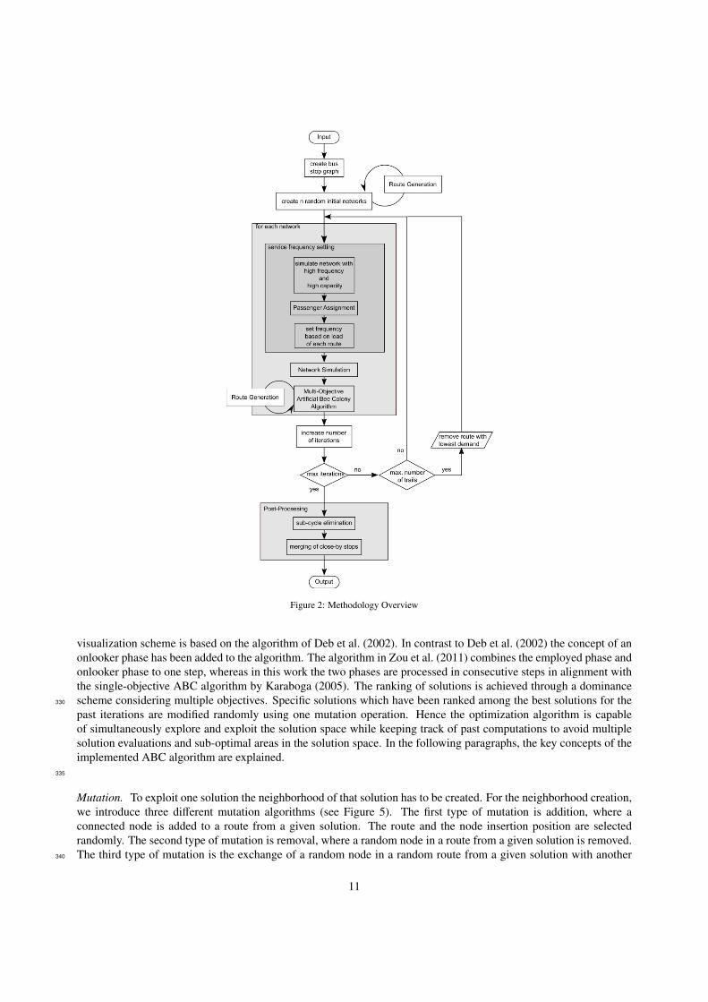
Figure 2: Methodology Overview

visualization scheme is based on the algorithm of Deb et al. (2002). In contrast to Deb et al. (2002) the concept of anonlooker phase has been added to the algorithm. The algorithm in Zou et al. (2011) combines the employed phase andonlooker phase to one step, whereas in this work the two phases are processed in consecutive steps in alignment withthe single-objective ABC algorithm by Karaboga (2005). The ranking of solutions is achieved through a dominancescheme considering multiple objectives. Specific solutions which have been ranked among the best solutions for the330

past iterations are modified randomly using one mutation operation. Hence the optimization algorithm is capableof simultaneously explore and exploit the solution space while keeping track of past computations to avoid multiplesolution evaluations and sub-optimal areas in the solution space. In the following paragraphs, the key concepts of theimplemented ABC algorithm are explained.

335

Mutation. To exploit one solution the neighborhood of that solution has to be created. For the neighborhood creation,we introduce three different mutation algorithms (see Figure 5). The first type of mutation is addition, where aconnected node is added to a route from a given solution. The route and the node insertion position are selectedrandomly. The second type of mutation is removal, where a random node in a route from a given solution is removed.The third type of mutation is the exchange of a random node in a random route from a given solution with another340

11

(a) Fully connected bus stopgraph; each node is one potentialbus stop

(b) One feasible network solutionincluding routes and served busstops.Route 1 (blue): 1-6-3Route 2 (red): 4-6-3

Figure 3: Example bus stop graph and a corresponding bee (solution)

P

scout phase

onlooker phaseemployed phase

EP

90%

10%

non-domination&

distancenew

mutation

focu

s

newold

muta

ted

dominance comparison

normalized values

non-domination&

distancefinal

Route Generationto fill up

Figure 4: Overview over multi-objective artificial bee colony algorithm (MOABC)

feasible node to guarantee connectivity. With these three steps, it can be guaranteed that the created neighborhoodsolutions are similar to the initial solution and therefore locally exploit the solution space. The choice of mutationis random. This procedure restricts the attention to simple neighborhood moves in the space of feasible solutions,whereas the removal of the route with the lowest passenger load allows for larger moves in the solution space. Theremoval of a route is done after a certain number of trail computations have been computed (see Figure 2).345

Crowding distance and dominance. Since the multi-objective problem formulation does not allow for a single com-pensatory fitness computation, the ranking of solutions is done in a two-step approach. First, a fast non-dominatedsorting algorithm is used to find non-dominated solutions and create different levels of non-dominated fronts (Figure6). A solution (bee1) is said to dominate another solution (bee2) if all objective values are smaller or equal and at leastone objective value is smaller than in the other solution. For simplicity reasons only two out of the three objectives350

are visualized in Figure 6. In this example two levels of non-dominated fronts have been computed. The second stepis the computation of the crowding distance. The crowding distance for a solution is the summation overall objectivesof the mean distance between the neighboring solutions. With the computation of the crowding distance a measure forthe diversity of each point is generated. The final ranking of the solutions is done with the combination of both metrics(see Algorithm 1). The solutions of the same non-dominated front are sorted based on their crowding distance value.355

The larger the distance, the higher the solution is ranked. This is done to increase the heterogeneity of the investigatedsolutions. If the divergence would be low the solutions would not explore the entire range of the non-dominated front.

12

(a) Mutation to add a node to aroute.Route 1 (blue): 2-1-6-3Route 2 (red): 4-6-3Route 3 (green): walking

(b) Mutation to remove a nodefrom a route.Route 1 (blue): 1-3Route 2 (red): 4-6-3Route 3 (green): walking

(c) Mutation to exchange a nodewithin a route.Route 1 (blue): 1-6-3Route 2 (red): 4-2-3Route 3 (green): walking

Figure 5: Neighborhood definition and mutation creation algorithms for MOABC

f1

f2 solutions

front

extremesolution

distance

extremesolution

i

i+1

i-1

Figure 6: Non-dominated sorting and diversity computation

Algorithm 1 Sorting based on Dominance and Crowding Distance

Require: Non-dominated fronts (F j) with j as the level of each front & crowding distance (di where i ∈ F j)Initiate vector

(vsorted ∈ R1×P

)for f in F j do

tmpsorted = reverse sort (di) i ∈ f {sort crowding distance from high to low}append tmpsorted to vsorted

end for

Employed bee phase. Based on the non-dominated and crowding distance sorting, we select the 90% best solutionsas employed bees. If the total population is denoted as P the number of bees in the system at this step is εP = 0.9 · P.360

Each employed bee solution is mutated resulting in a total number of 2εP. Each mutated solution is compared with theoriginal solution using Algorithm 2. If the mutated solution is dominating the original solution, the mutation replacesthe original solution. If the original solution dominates the mutation the original solution stays in the population. Ifnone of the two solutions is dominated by the other one, we pick one of the two solutions at random and sort thatsolution in the population. After the employed bee phase the total number of bees in the population is again εP.365

13

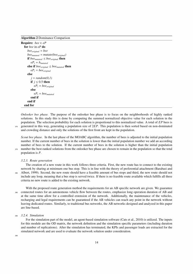
Algorithm 2 Dominance Comparison

Require: bee ∈ εPfor bee in εP do

beeoriginal = beebeemutated = mutate(beeoriginal)if beemutated � beeoriginal thenεPi = bmutated

else if beeoriginal � beemutated thenεPi = beeoriginal

elsej = random(0,1)if j ≤ 0.5 thenεPi = beeoriginal

elseεPi = beemutated

end ifend if

end for

Onlooker bee phase. The purpose of the onlooker bee phase is to focus on the neighborhoods of highly rankedsolutions. In this study this is done by computing the summed normalized objective value for each solution in thepopulation. The selection probability for each solution is proportional to this normalized value. A total of EP bees isgenerated in this way, generating a population size of 2EP. This population is then sorted based on non-dominated370

and crowding distance and only the solutions of the first front are kept in the population.

Scout bee phase. In the last phase of the MOABC algorithm, the number of bees is adjusted to the initial populationnumber. If the current number of bees in the solution is lower than the initial population number we add an accordingnumber of bees to the solution. If the current number of bees in the solution is higher than the initial populationnumber the best-ranked solutions from the onlooker bee phase are chosen to remain in the population so that the total375

population is P.

3.2.3. Route generationThe creation of a new route in this work follows three criteria. First, the new route has to connect to the existing

network by sharing at minimum one bus stop. This is in line with the theory of preferential attachment (Barabasi andAlbert, 1999). Second, the new route should have a feasible amount of bus stops and third, the new route should not380

include any loop, meaning that a bus stop is served twice. If there is no feasible route available which fulfills all threecriteria no new route is added to the existing network.

With the proposed route generation method the requirements for an AB specific network are given. We guaranteeconnected routes for an autonomous vehicle flow between the routes, emphasize long operation duration of AB and385

at the same time allow for a controlled extension of the network. Additionally, the maintenance of the vehicles,recharging and legal requirements can be guaranteed if the AB vehicles can reach any point in the network withoutleaving dedicated routes. Similarly, to traditional bus networks, the AB networks designed and analyzed in this paperare line-based.

3.2.4. Simulation390

For the simulation part of the model, an agent-based simulation software (Cats et al., 2010) is utilized. The inputsfor this module are the OD matrix, the network definition and the simulation specific parameters (including durationand number of replications). After the simulation has terminated, the KPIs and passenger loads are extracted for thesimulated network and are used to evaluate the network solution under consideration.

395

14

The simulation software incorporates a dynamic public transport assignment model. The simulation of operationsconsiders several transit-related parameters, e.g. bus routes, level of demand, PT schedule, locations of bus stops andmore. A schedule-based assignment model was chosen to realistically capture the different ranges of potential servicefrequencies. Additionally, the presented results are not dependent on the detailed schedule the vehicles operate on.This affects waiting times at transfers in the network. Since the resulting networks are simple and have only few lines400

this negative effect can be neglected. In this model, passenger route choices and vehicle travel times are stochastic.The passenger assignment model includes within-day and day-to-day dynamics (Cats and West, 2020). A randomutility model determines the passenger’s path choice decisions. The utility of each potential path, from the currentposition to the trip’s destination, for every passenger is evaluated based on the expected waiting time, in-vehicle time,walking time and number of transfers. These metrics are computed based on real-time transit information and the405

current bus schedule. The utility of an action is calculated as the logsum of the utilities of all paths available giventhis action. The final decision is made based on the probability distribution as given in equation 11, where pt,k is theprobability for action t ∈ T of passenger k based on the utility ut,k for action t and passenger k.

pt,k =eut,k∑

i∈T eui,k(11)

The day-to-day dynamics fuse the passengers experienced travel times from a previous day with the expected410

travel times using a Markov decision process. With this simulation, the resulting load profile of a given PT network isthe outcome of service reliability, on-board crowding and real-time information which makes it possible to analyze thedynamic passenger load distribution resulting from various service configurations. The final outputs of the simulationmodel are averaged values of ensemble runs of the same scenario. By that stochastic decisions in the simulation modelare accounted for.415

3.2.5. Post-processingThe post-processing steps aim at creating more practically applicable and realistic solutions. In order to achieve

this two sequential steps have been implemented. The first is a basic sub-cycle elimination routine, and the secondstep merges nearby served bus stops. Each of these steps creates a child solution which is evaluated by re-simulation420

and computation of the objective values. The child solution is accepted as a new solution if it dominates its parent.The output of the post-processing step are the final proposed solutions to the network design problem.

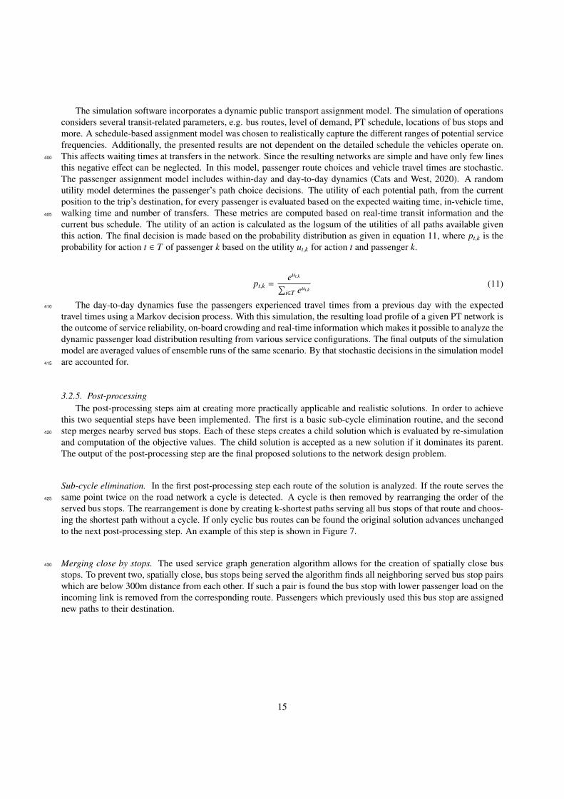
Sub-cycle elimination. In the first post-processing step each route of the solution is analyzed. If the route serves thesame point twice on the road network a cycle is detected. A cycle is then removed by rearranging the order of the425

served bus stops. The rearrangement is done by creating k-shortest paths serving all bus stops of that route and choos-ing the shortest path without a cycle. If only cyclic bus routes can be found the original solution advances unchangedto the next post-processing step. An example of this step is shown in Figure 7.

Merging close by stops. The used service graph generation algorithm allows for the creation of spatially close bus430

stops. To prevent two, spatially close, bus stops being served the algorithm finds all neighboring served bus stop pairswhich are below 300m distance from each other. If such a pair is found the bus stop with lower passenger load on theincoming link is removed from the corresponding route. Passengers which previously used this bus stop are assignednew paths to their destination.

15

(a) Network design before sub-cycle elimination (b) Network design after sub-cycle elimination

Figure 7: Illustrative example of the sub-cycle elimination post-processing step

4. Case study435

The modeling framework is used to design a new PT network for Barkarby, located in the northern part of Stock-holm and connected with the city center by train. To match current travel demand and connect residents with theexisting PT system a line-based AB service is operated since the beginning of 2019. However, due to the building ofnew residential areas and an industrial park, the daily number of trips is expected to increase to approximately 10000in 2025. Therefore, an extension and redesign of the exiting PT system is required, including a larger line-based440

AB network in combination with a new metro line. The proposed framework allows incorporating changed circum-stances, e.g. new road network, increased demand, and integration of new metro stations in the existing PT system.Furthermore, it allows evaluating the effect of different vehicle technologies on the provided level of service in the area.

Input data. The framework requires three main sets of input data: the road network, the demand rate per hour445

in origin-destination matrix form and the potential bus stop locations. The road network is extracted using Open-StreetMap data (OpenStreetMap, 2017). An additional pre-processing step is applied to remove non-drivable roads,e.g. narrow roads, complex intersections and private sections. The pre-processing step is specifically relevant forthe operation of AB. Due to regulatory, legislative and technical constraints AB are currently not able to operate onall existing roads. The filtering of drivable roads is done based on input from the local authorities. The demand is450

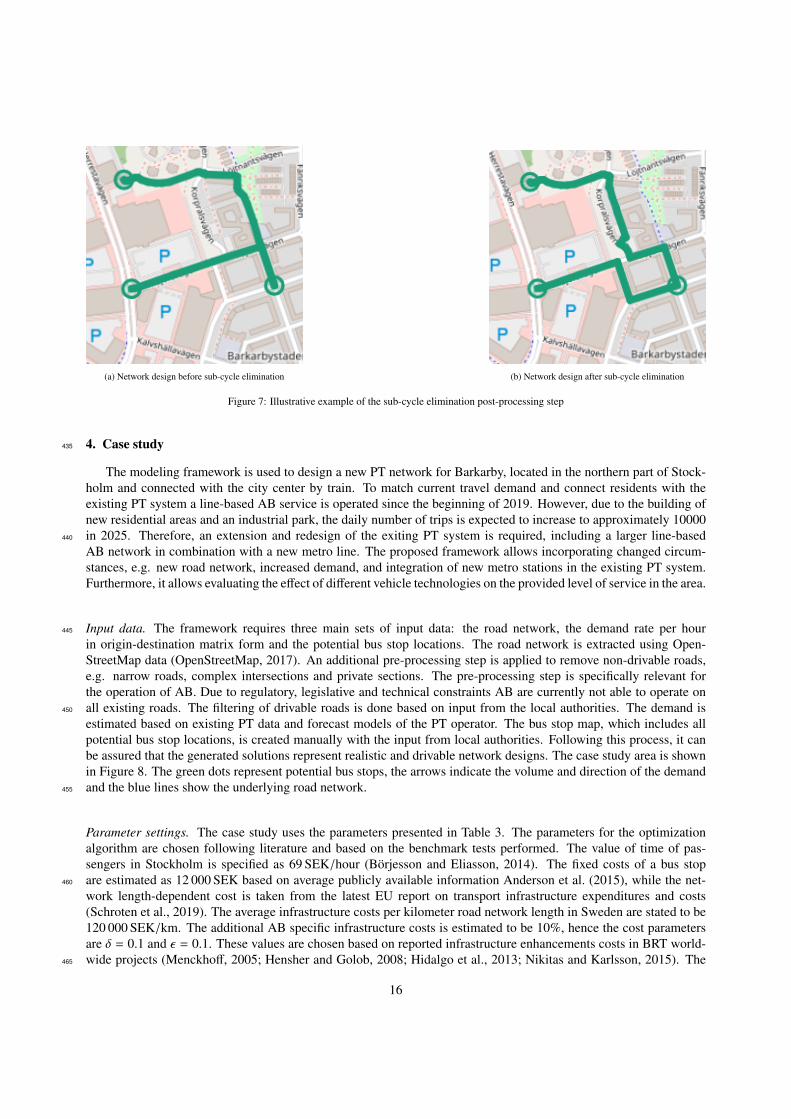
estimated based on existing PT data and forecast models of the PT operator. The bus stop map, which includes allpotential bus stop locations, is created manually with the input from local authorities. Following this process, it canbe assured that the generated solutions represent realistic and drivable network designs. The case study area is shownin Figure 8. The green dots represent potential bus stops, the arrows indicate the volume and direction of the demandand the blue lines show the underlying road network.455

Parameter settings. The case study uses the parameters presented in Table 3. The parameters for the optimizationalgorithm are chosen following literature and based on the benchmark tests performed. The value of time of pas-sengers in Stockholm is specified as 69 SEK/hour (Borjesson and Eliasson, 2014). The fixed costs of a bus stopare estimated as 12 000 SEK based on average publicly available information Anderson et al. (2015), while the net-460

work length-dependent cost is taken from the latest EU report on transport infrastructure expenditures and costs(Schroten et al., 2019). The average infrastructure costs per kilometer road network length in Sweden are stated to be120 000 SEK/km. The additional AB specific infrastructure costs is estimated to be 10%, hence the cost parametersare δ = 0.1 and ε = 0.1. These values are chosen based on reported infrastructure enhancements costs in BRT world-wide projects (Menckhoff, 2005; Hensher and Golob, 2008; Hidalgo et al., 2013; Nikitas and Karlsson, 2015). The465

16

Building

Bus Stop

Infrastructure Graph

OpenStreetMap©

Figure 8: Representation of the case study including an abstraction of the input values.

accuracy of these additional cost estimations has to be seen as low due to the lack of available data. In this study, theabsolute cost values are not of critical importance as, the multi-objective problem formulation allows for an impactstudy based on infrastructure cost changes.

The internal simulation parameters are based on the values reported in Cats (2013). The vehicle capacity is set to470

match the AB currently operating in the residential area as part of a pilot study. To account for statistical variations thefinal variable value is the mean value of five individual simulations. The required number of replications is computedaccording to the work by Burghout (2004) and Dowling et al. (2004). To account for the stochastic nature of theMOABC the final results presented are the averaged values over 10 full framework iterations. The visualized finalnetwork designs are the best from all simulation results.475

17

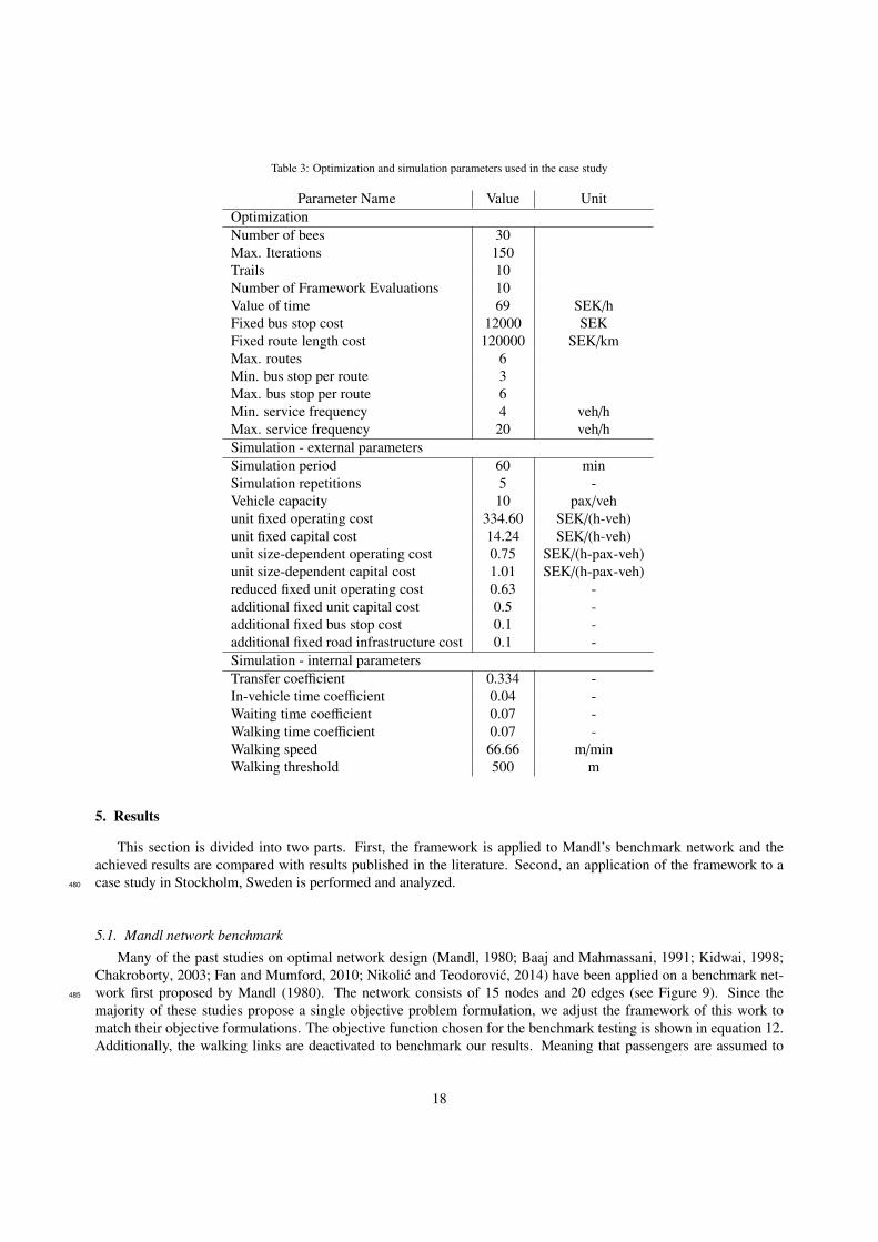
Table 3: Optimization and simulation parameters used in the case study

Parameter Name Value UnitOptimizationNumber of bees 30Max. Iterations 150Trails 10Number of Framework Evaluations 10Value of time 69 SEK/hFixed bus stop cost 12000 SEKFixed route length cost 120000 SEK/kmMax. routes 6Min. bus stop per route 3Max. bus stop per route 6Min. service frequency 4 veh/hMax. service frequency 20 veh/hSimulation - external parametersSimulation period 60 minSimulation repetitions 5 -Vehicle capacity 10 pax/vehunit fixed operating cost 334.60 SEK/(h-veh)unit fixed capital cost 14.24 SEK/(h-veh)unit size-dependent operating cost 0.75 SEK/(h-pax-veh)unit size-dependent capital cost 1.01 SEK/(h-pax-veh)reduced fixed unit operating cost 0.63 -additional fixed unit capital cost 0.5 -additional fixed bus stop cost 0.1 -additional fixed road infrastructure cost 0.1 -Simulation - internal parametersTransfer coefficient 0.334 -In-vehicle time coefficient 0.04 -Waiting time coefficient 0.07 -Walking time coefficient 0.07 -Walking speed 66.66 m/minWalking threshold 500 m

5. Results

This section is divided into two parts. First, the framework is applied to Mandl’s benchmark network and theachieved results are compared with results published in the literature. Second, an application of the framework to acase study in Stockholm, Sweden is performed and analyzed.480

5.1. Mandl network benchmark

Many of the past studies on optimal network design (Mandl, 1980; Baaj and Mahmassani, 1991; Kidwai, 1998;Chakroborty, 2003; Fan and Mumford, 2010; Nikolic and Teodorovic, 2014) have been applied on a benchmark net-work first proposed by Mandl (1980). The network consists of 15 nodes and 20 edges (see Figure 9). Since the485

majority of these studies propose a single objective problem formulation, we adjust the framework of this work tomatch their objective formulations. The objective function chosen for the benchmark testing is shown in equation 12.Additionally, the walking links are deactivated to benchmark our results. Meaning that passengers are assumed to

18

always board the bus, if the bus stop is served by a vehicle.490

min: Z = α

i=n−1∑i=1

j=n∑j=i+1

di j pi j + β

i=n−1∑i=1

j=n∑j=i+1

di jti j (12)

The problem is constrained by (1) a maximum route length, (2) a connected network, (3) minimum number ofnodes per route, (4) each route is free of cycles and backtracks. In equation 12 α and β are weights for the two terms.The first term describes the path length pi j between the two nodes i, j ∈ N multiplied by the demand di j betweenthese two nodes. The second term describes the number of transfers ti j per path between the nodes multiplied bythe corresponding demand. This reduces the problem complexity since no passenger travel costs components such495

as in-vehicle times, walking time, waiting times and infrastructure costs are considered. Additionally, the objectivefunction is based on a single objective rather than on multiple objectives as proposed in equation 5. This limits theapplicability for more complex problems as presented in section 4. However, the quality of the benchmark results canstill be transferred to the complex case since the same heuristics and algorithms are used in both cases.

500

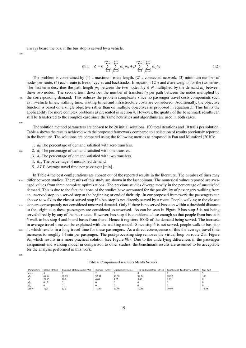
The solution method parameters are chosen to be 20 initial solutions, 100 total iterations and 10 trails per solution.Table 4 shows the results achieved with the proposed framework compared to a selection of results previously reportedin the literature. The solutions are compared using the following metrics as proposed in Fan and Mumford (2010):

1. d0 The percentage of demand satisfied with zero transfers.2. d1 The percentage of demand satisfied with one transfer.505

3. d2 The percentage of demand satisfied with two transfers.4. dun The percentage of unsatisfied demand.5. ATT Average travel time per passenger [min].

In Table 4 the best configurations are chosen out of the reported results in the literature. The number of lines maydiffer between studies. The results of this study are shown in the last column. The numerical values reported are aver-510

aged values from three complete optimizations. The previous studies diverge mostly in the percentage of unsatisfieddemand. This is due to the fact that none of the studies have accounted for the possibility of passengers walking froman unserved stop to a served stop at the beginning or end of their trip. In our proposed framework the passengers canchoose to walk to the closest served stop if a bus stop is not directly served by a route. People walking to the closeststop are consequently not considered unserved demand. Only if there is no served bus stop within a threshold distance515

to the origin stop these passengers are considered as unserved. As can be seen in Figure 9 bus stop 5 is not beingserved directly by any of the bus routes. However, bus stop 4 is considered close enough so that people from bus stop5 walk to bus stop 4 and board buses from there. Hence it registers 100% of the demand being served. The increasein average travel time can be explained with the walking model. Since stop 5 is not served, people walk to bus stop4, which results in a long travel time for these passengers. As a direct consequence of this the average travel time520

increases to roughly 14 min per passenger. The post-processing step removes the virtual loop on route 2 in Figure9a, which results in a more practical solution (see Figure 9b). Due to the underlying differences in the passengerassignment and walking model in comparison to other studies, the benchmark results are assumed to be acceptablefor the analysis performed in this work.

525

Table 4: Comparison of results for Mandls Network

Parameters Mandl (1980) Baaj and Mahmassani (1991) Kidwai (1998) Chakroborty (2003) Fan and Mumford (2010) Nikolic and Teodorovic (2014) Our bestnlines 4 7 7 8 8 8 5d0 69.94 80.99 93.91 90.38 94.54 98.97 100d1 29.93 19.01 6.09 9.62 5.46 1.03 0d2 0.13 0 0 0 0 0 0dun 0 0 0 0 0 0 0ATT 12.9 12.5 10.69 10.46 10.36 10.09 14.35

19

(a) Network solution without post-processing

Route 1: 11, 10, 7

Route 2: 12, 4, 2, 3, 8, 15

Route 3: 4, 2, 1

Route 4: 14, 13, 9

Route 5: 6, 2, 1

1

23

45

6

7

8

9

10

11

12

13

14

15

(b) Network solution with post-processing

Figure 9: Best network solution of the proposed framework on Mandl’s network

5.2. Case study analysis

In Figure 10 the hypervolume convergence is shown for the AB optimization and the conventional bus opti-mization scenario. After 150 iterations the optimization is terminated. The number of iterations was determined intwo ways. In other studies that solve similar-sized problems approximately 150 iterations are reported as sufficientfor convergence (see Zou et al. (2011); Szeto and Jiang (2014)). Second, the analysis of the benchmark problem530

allowed to approximate a reasonable number of iterations required to achieve a converging solution. Besides thenumber of iterations also the number of function evaluations must be considered to evaluate convergence. Using theparameters from Table 3 the average number of function evaluations for one optimization run can be estimated to150 · (0.5 · 30 · 2) · (0.1 · 30) = 13500; where 150 is the number of iterations and 30 the number of bees; 0.5 · 30 is thenumber of evaluations for each employed phase and onlooker phase assuming a mutation and focus rate of 50%, and535

0.1 · 30 equals the evaluations in each scout phase assuming ε = 0.9. From Figure 10 it can be seen that the problemconverges step-wise for both, the AB and conventional bus, cases. The steps can be explained by the removal of buslines with low passenger load in the candidate solutions after a certain number of iterations. After approximately 90iterations the hypervolume starts to slightly diverge again, and additionally the noise between computation repetitionsincreases. Both of these can be explained by the random search characteristics of the MOABC and the line removal540

procedure. New random candidate solutions are generated after each iteration; these solutions are created with ahigh number of lines resulting in a higher objective value. Additionally, in each iteration, approximately 50% of thesolutions are mutated or slightly varied which can lead to an improved or deteriorated solution. Towards the end ofthe optimization, the probability that a mutated solution is worse than the mean average of all bees is increasing since50% of these solutions are the best solutions achieved through the previous iterations. Hence the mean average is545

more likely to fluctuate and more likely to increase towards later iterations. The overall best solutions are not affectedby this phenomenon.

20

0 20 40 60 80 100 120 140

Iterat ion

6.8

6.9

7.0

7.1

Hy

pe

rvo

lum

e

1e� 19 Autonom ous Technology Operat ion

m ean HV

single run HV

(a) Hypervolume convergence for the AB deployment

0 20 40 60 80 100 120 140

Iterat ion

2.12

2.14

2.16

2.18

2.20

2.22

2.24

Hy

pe

rvo

lum

e

1e� 19 Convent ional Technology Operat ion

m ean HV

single run HV

(b) Hypervolume convergence for the conventional bus deployment

Figure 10: Hypervolume convergence for the AB deployment scenario and for conventional bus deployment scenario. The reference point is set tobe the origin. The colors are the hypervolume curves for a single framework iteration. The blue line is the mean of all 10 ensemble runs.

(a) User-focused network design withconventional buses.

(b) User-focused network design withautonomous buses.

(c) Operator-focused network designwith conventional buses.

(d) Operator-focused network designwith autonomous buses.

Figure 11: Maps (a) and (b) show the computed user-focused design for conventional and autonomous buses respectively, while (c) and (d) showthe operator-focused design for conventional and autonomous buses.

5.3. User-focused and operator-focused design

In contrast to the benchmark analysis, the case study framework is implemented as a MOABC. In the following550

analysis the difference between user-focused and operator-focused network designs are presented. In Figure 11 thenumerical values for the specific solutions are given. The values belong to to one solution each. The solutions areachieved by computing the Pareto front using the concept of non-domination and then sorting these solutions eitherfor minimum user cost or minimum operator cost respectively. In general the inclusion of walking as an alternativemode of transport has a big impact on the network design and achieved results. Comparing the total number of people555

walking with the number of people boarding a bus clearly shows the significance of walking in this case study. Basedon the spatial size of the case scenario walking is a valuable option for many passengers and is therefore selectedby the majority of travelers. Nevertheless, two distinct network designs are identifiable. The user-focused design(see Figure 11a and 11b) is characterized by higher operating costs and higher infrastructure costs compared to theoperator-focused design. This is the direct consequence of the higher number of bus stops and networks in the public560

transport network. The larger network length and the higher number of bus stops leads to a better accessibility for

21

Table 5: Results for user-focused and operator-focused network design solutions, the values represent the non-dominated solution

User-focused Operator-focused Local Operatorautonomous conventional autonomous conventional autonomous

ObjectivesUser Cost [SEK] 13500 13600 13700 13700 16200

Operator Cost [SEK/h] 326 733 163 366 488Infrastructure Cost [SEK] 81400 73000 40600 36700 79900

KPIWalking only trips 10211 10313 10367 10398 9963

Bus Passenger 206 105 95 26 538Denied Passenger Boardings 10 2 12 0 290

Weighted in-vehicle Time [sec/pax] 69 68 88 39 101In-vehicle Time [sec/pax] 59 62 74 40 75

Waiting time [sec/pax] 491 470 591 423 1050Access Time [sec/pax] 94 52 179 211 50

Waiting time due to denied boarding [sec/pax] 52 17 151 0 912Direct Walking Time [sec/pax] 974 979 976 980 981

Total Walking time[sec/pax] 956 969 969 978 933Number of Transfers 0 0 0 0 0

Average Frequency 4 4 4 4 4Number of Lines 2 2 1 1 1

Number of Bus stops 6 6 3 3 6Total Route length [m] 5646 2608 2594 1903 1820

passenger in to the public transport network, therefore resulting in more boarding passengers, and shorter access timesper passenger. Additionally, it can be seen that the level of crowding is low, since the difference between recordedin-vehicle time and perceived in-vehicle time is marginal. Interestingly, the in-vehicle time per passenger, waitingtime ans service frequency per line are similar for both, the user-focused and operator-focused design. The service565

frequency of 4 veh/h indicates the competitiveness of walking in this case study and additionally the low supply uti-lization. Furthermore, no transfers could be registered, indicating that passengers take direct trips from their origin todestination. The solution in Figure 11b shows a large overlap of route 1 and 2. Route 1 seemingly goes in a loop fromnorth to south and back north. This network however was not dominated by a post-processed solution and is thereforepresented as is. The solution in Figure 11a could be improved through the post-processing step by merging one bus570

stop and removing several virtual loops.

The operator-focused network (see Figure 11c and 11d) is characterized by fewer, shorter lines and few bus stops.This results in lower infrastructure costs compared to the user-driven design. Additionally, the operator-focused de-sign leads to increased access times and long waiting times due to denied boarding.575

22

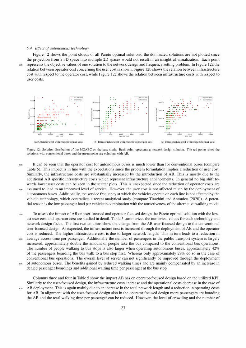
5.4. Effect of autonomous technology

Figure 12 shows the point clouds of all Pareto optimal solutions, the dominated solutions are not plotted sincethe projection from a 3D space into multiple 2D spaces would not result in an insightful visualization. Each pointrepresents the objective values of one solution to the network design and frequency setting problem. In Figure 12a the580

relation between operator cost concerning the user cost is shown, Figure 12b shows the relation between infrastructurecost with respect to the operator cost, while Figure 12c shows the relation between infrastructure costs with respect touser costs.

15000 20000 25000 30000 35000User Cost

0

1000

2000

3000

4000

Operator Cost

conventionalautonomous

(a) Operator cost with respect to user cost

0 1000 2000 3000 4000Operator Cost

50000

100000

150000

200000

Infra

structure Co

st

conventionalautonomous

(b) Infrastructure cost with respect to operator cost

15000 20000 25000 30000 35000User Cost

50000

100000

150000

200000

Infra

structure Co

st

conventionalautonomous

(c) Infrastructure cost with respect to user cost

Figure 12: Solution distribution of the MOABC on the case study. Each point represents a network design solution. The red points show thesolutions with conventional buses and the green points are solutions with AB.

It can be seen that the operator cost for autonomous buses is much lower than for conventional buses (compare585

Table 5). This impact is in line with the expectations since the problem formulation implies a reduction of user cost.Similarly, the infrastructure costs are substantially increased by the introduction of AB. This is mostly due to theadditional AB specific infrastructure costs which represent infrastructure enhancements. In general no big shift to-wards lower user costs can be seen in the scatter plots. This is unexpected since the reduction of operator costs areassumed to lead to an improved level of service. However, the user cost is not affected much by the deployment of590

autonomous buses. Additionally, the service frequency at which the vehicles operate on each line is not affected by thevehicle technology, which contradicts a recent analytical study (compare Tirachini and Antoniou (2020)). A poten-tial reason is the low passenger load per vehicle in combination with the attractiveness of the alternative walking mode.

To assess the impact of AB on user-focused and operator-focused design the Pareto optimal solution with the low-595

est user cost and operator cost are studied in detail. Table 5 summarizes the numerical values for each technology andnetwork design focus. The first two columns show the change from the AB user-focused design to the conventionaluser-focused design. As expected, the infrastructure cost is increased through the deployment of AB and the operatorcost is reduced. The higher infrastructure cost is due to larger network length. This in turn leads to a reduction inaverage access time per passenger. Additionally the number of passengers in the public transport system is largely600

increased, approximately double the amount of people take the bus compared to the conventional bus operations.The number of people walking to bus stops is also larger when operating autonomous buses, approximately 42%of the passengers boarding the bus walk to a bus stop first. Whereas only approximately 29% do so in the case ofconventional bus operations. The overall level of server can not significantly be improved through the deploymentof autonomous buses. The benefits gained by reduced walking times and are mainly compensated by an increase in605

denied passenger boardings and additional waiting time per passenger at the bus stop.

Columns three and four in Table 5 show the impact AB has on operator-focused design based on the utilized KPI.Similarly to the user-focused design, the infrastructure costs increase and the operational costs decrease in the case ofAB deployment. This is again mainly due to an increase in the total network length and a reduction in operating costs610

for AB. In alignment with the user-focused design also in the operator focused design more passengers are boardingthe AB and the total walking time per passenger can be reduced. However, the level of crowding and the number of

23

denied passenger boardings are significantly higher in the case of autonomous bus, which in turn leads to a deteriora-tion in the level of service.

615

It is concluded that while the introduction of AB on line-based PT networks does not improve the level of serviceacross the board, a slight improvement can be identified in the user-focused designs. However, due to a larger networklength and shorter walking times more passengers can be attracted to the public transport system when operating AB.In the presented case study approximately 2-3 more passengers can be expected to board when the buses operateautonomously as opposed to humanly-driven buses.620

0

5000

10000

15000

20000

25000

30000

1 2 3 4 5 6

Use

r C

ost

[S

EK

]

Number of Lines

autonomous

conventional

(a) Change of user cost

0

500

1000

1500

2000

2500

3000

3500

4000

1 2 3 4 5 6

Op

erat

or

Co

st [

SE

K/h

]

Number of Lines

autonomous

conventional

(b) Change of operator cost

0

50000

100000

150000

200000

250000

300000

1 2 3 4 5 6

Infr

astr

uct

ure

Co

st [

SE

K]

Number of Lines

autonomous

conventional

(c) Change of infrastructure cost

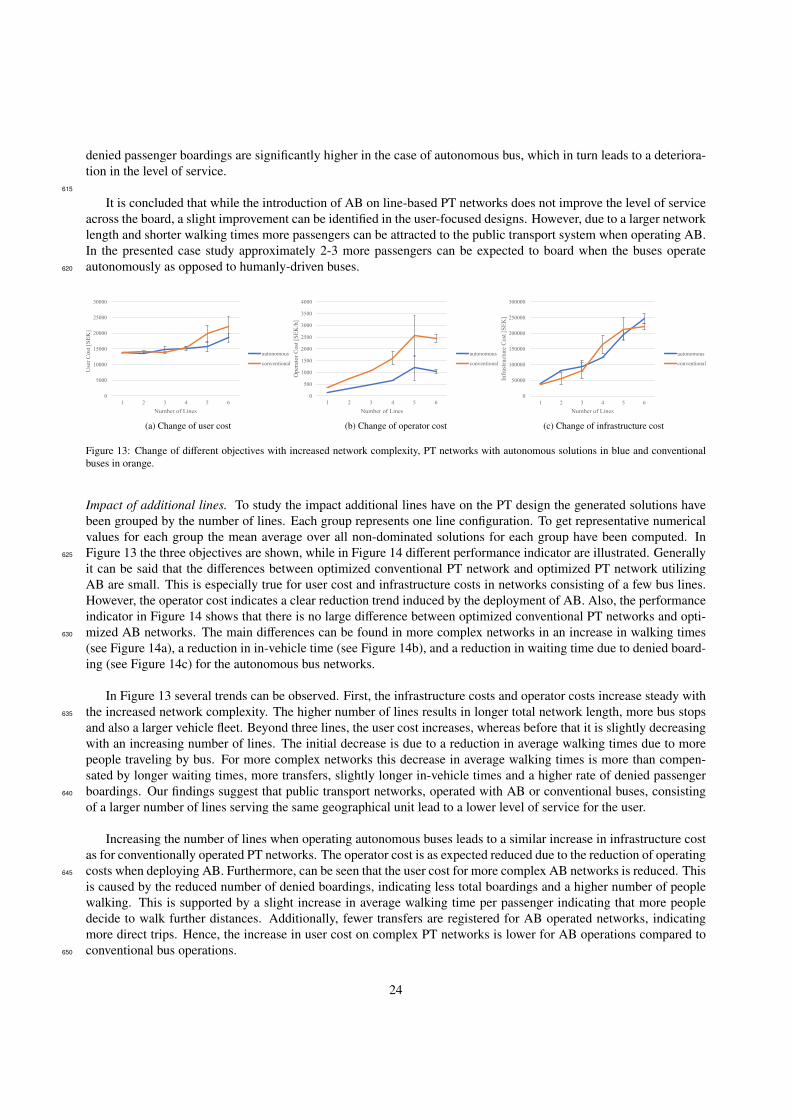
Figure 13: Change of different objectives with increased network complexity, PT networks with autonomous solutions in blue and conventionalbuses in orange.

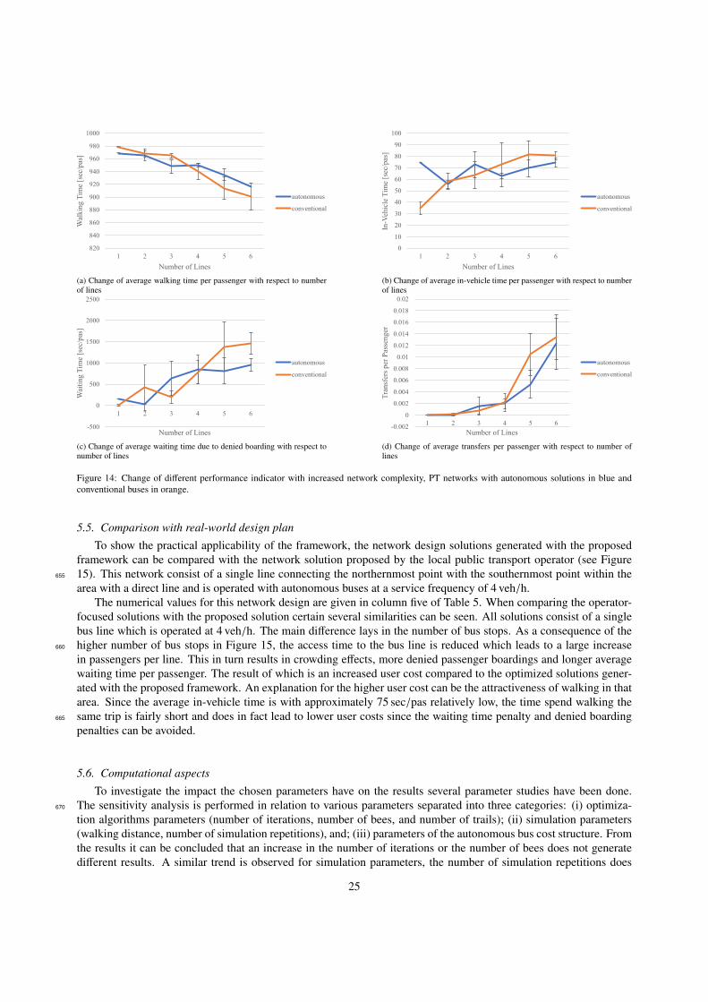
Impact of additional lines. To study the impact additional lines have on the PT design the generated solutions havebeen grouped by the number of lines. Each group represents one line configuration. To get representative numericalvalues for each group the mean average over all non-dominated solutions for each group have been computed. InFigure 13 the three objectives are shown, while in Figure 14 different performance indicator are illustrated. Generally625

it can be said that the differences between optimized conventional PT network and optimized PT network utilizingAB are small. This is especially true for user cost and infrastructure costs in networks consisting of a few bus lines.However, the operator cost indicates a clear reduction trend induced by the deployment of AB. Also, the performanceindicator in Figure 14 shows that there is no large difference between optimized conventional PT networks and opti-mized AB networks. The main differences can be found in more complex networks in an increase in walking times630

(see Figure 14a), a reduction in in-vehicle time (see Figure 14b), and a reduction in waiting time due to denied board-ing (see Figure 14c) for the autonomous bus networks.

In Figure 13 several trends can be observed. First, the infrastructure costs and operator costs increase steady withthe increased network complexity. The higher number of lines results in longer total network length, more bus stops635

and also a larger vehicle fleet. Beyond three lines, the user cost increases, whereas before that it is slightly decreasingwith an increasing number of lines. The initial decrease is due to a reduction in average walking times due to morepeople traveling by bus. For more complex networks this decrease in average walking times is more than compen-sated by longer waiting times, more transfers, slightly longer in-vehicle times and a higher rate of denied passengerboardings. Our findings suggest that public transport networks, operated with AB or conventional buses, consisting640

of a larger number of lines serving the same geographical unit lead to a lower level of service for the user.

Increasing the number of lines when operating autonomous buses leads to a similar increase in infrastructure costas for conventionally operated PT networks. The operator cost is as expected reduced due to the reduction of operatingcosts when deploying AB. Furthermore, can be seen that the user cost for more complex AB networks is reduced. This645

is caused by the reduced number of denied boardings, indicating less total boardings and a higher number of peoplewalking. This is supported by a slight increase in average walking time per passenger indicating that more peopledecide to walk further distances. Additionally, fewer transfers are registered for AB operated networks, indicatingmore direct trips. Hence, the increase in user cost on complex PT networks is lower for AB operations compared toconventional bus operations.650

24

820

840

860

880

900

920

940

960

980

1000

1 2 3 4 5 6

Wal

kin

g T

ime

[sec

/pas

]

Number of Lines

autonomous

conventional

(a) Change of average walking time per passenger with respect to numberof lines

0

10

20

30

40

50

60

70

80

90

100

1 2 3 4 5 6

In-V

ehic

le T

ime

[sec

/pas

]

Number of Lines

autonomous

conventional

(b) Change of average in-vehicle time per passenger with respect to numberof lines

-500

0

500

1000

1500

2000

2500

1 2 3 4 5 6

Wai

tin

g T

ime

[sec

/pas

]

Number of Lines

autonomous

conventional

(c) Change of average waiting time due to denied boarding with respect tonumber of lines

-0.002

0

0.002

0.004

0.006

0.008

0.01

0.012

0.014

0.016

0.018

0.02

1 2 3 4 5 6

Tra

nsf

ers

per

Pas

sen

ger

Number of Lines

autonomous

conventional

(d) Change of average transfers per passenger with respect to number oflines

Figure 14: Change of different performance indicator with increased network complexity, PT networks with autonomous solutions in blue andconventional buses in orange.

5.5. Comparison with real-world design plan

To show the practical applicability of the framework, the network design solutions generated with the proposedframework can be compared with the network solution proposed by the local public transport operator (see Figure15). This network consist of a single line connecting the northernmost point with the southernmost point within the655

area with a direct line and is operated with autonomous buses at a service frequency of 4 veh/h.The numerical values for this network design are given in column five of Table 5. When comparing the operator-

focused solutions with the proposed solution certain several similarities can be seen. All solutions consist of a singlebus line which is operated at 4 veh/h. The main difference lays in the number of bus stops. As a consequence of thehigher number of bus stops in Figure 15, the access time to the bus line is reduced which leads to a large increase660

in passengers per line. This in turn results in crowding effects, more denied passenger boardings and longer averagewaiting time per passenger. The result of which is an increased user cost compared to the optimized solutions gener-ated with the proposed framework. An explanation for the higher user cost can be the attractiveness of walking in thatarea. Since the average in-vehicle time is with approximately 75 sec/pas relatively low, the time spend walking thesame trip is fairly short and does in fact lead to lower user costs since the waiting time penalty and denied boarding665

penalties can be avoided.

5.6. Computational aspects

To investigate the impact the chosen parameters have on the results several parameter studies have been done.The sensitivity analysis is performed in relation to various parameters separated into three categories: (i) optimiza-670

tion algorithms parameters (number of iterations, number of bees, and number of trails); (ii) simulation parameters(walking distance, number of simulation repetitions), and; (iii) parameters of the autonomous bus cost structure. Fromthe results it can be concluded that an increase in the number of iterations or the number of bees does not generatedifferent results. A similar trend is observed for simulation parameters, the number of simulation repetitions does

25

Figure 15: Proposed network by the local public transport operator

not significantly impact the results. However, an increase in the walking threshold distance does lead to a reduction675

in ridership and therefore reduces the overall network length, a decrease of the threshold has the opposite effect onthe network length. Based on the multi-objective problem formulation the cost parameters for AB are not directlyinfluencing the other objective values, therefore a change in them does not lead to different conclusions but rather todifferent absolute values for the operational costs in the results.

680

The total computation time for the framework for one vehicle technology is approximately 72 h. This time in-cludes the 5 simulation repetitions per solution and an ensemble run of total 10 individual optimization runs. Theevaluation of one network solution including within-day learning and five simulation runs takes approximately 30 sec.The code is not utilizing parallel computation of each ensemble run and can therefore be sped up. The hardware usedto run the code was an Intel i7-7820HQ CPU @2.90GHz and 16GM RAM.685

6. Discussion and Conclusion

In this work an AB specific transit network design and frequency setting (TNDFS) framework is presented. Theframework consists of a multi-objective optimization problem which allows computing the impacts AB has on mul-tiple stakeholders. A simulation model with a stochastic, dynamic schedule-based passenger assignment is used to690

evaluate a given network design and assigns passenger demand to available bus routes. The optimization problem issolved by utilizing a multi-objective artificial bee algorithm (MOABC). The presented framework incorporates ABcharacteristics by constraining network solutions to have connected bus routes, smaller vehicle capacities, consider-ing changed operator costs for AB and determining approximated infrastructure enhancement costs. Additionally, thenumber of bus stops per route is a decision variable in the problem formulation which allows for a more diverse bus695

route creation. With this framework, potential differences between autonomous bus transport systems and conven-tional bus transport systems can be investigated. The expected differences originate from the reduced operation costsfor autonomous vehicles. Additionally, the study provides insight into the characteristics of user-oriented and opera-tor oriented network design for fixed-line operations. The proposed framework is applied to a benchmark network to

26

show the applicability and the overall functionality and a real sized case study in Barkarby, Sweden.700

In small-scale geographical units, public transport and active modes are the two main travel alternatives. Themajority of the demand in our case study is distributed over direct walking connections from origin to destination.Furthermore, the comparison of the user-oriented and operator oriented AB network design is in line with expecta-tions. The user-focused network design is characterized by many bus stops and many lines, resulting in a reduction705

of the average walking time to a bus stop and reduced crowding. In contrast, the operator-oriented network designconsists of only a few lines. This results on one hand in a smaller required fleet and shorter cycle times, and on theother hand, the few lines increase the average waiting times considerably, which reduces the level of service for theuser.

710

In the presented case study the deployment of autonomous buses on fixed-line public transport networks leads toa reduction of operator costs and an increased infrastructure cost this is mainly due to the reduction in operating costsand an increase in total network length. As a direct consequence of the longer PT network the number of passengersboarding a bus is 2-3 times higher in the case of AB deployment compared to conventional PT systems. Consequently,crowding increases and in-vehicle times become longer. The user cost can not be reduced in all cases. Especially for715

smaller, simple networks with a few lines the differences between optimized PT networks using conventional busesand AB diminishes. For simple networks (e.g. one or two bus lines) the reduction of walking times is compensatedmainly with larger in-vehicles times and a higher number of denied passenger boardings. However, for more complexnetworks and user-focused design, autonomous technology leads to an improved level of service, due to a reductionin the number of denied boardings. Additionally, less waiting time due to denied boarding and shorter in-vehicle time720

is registered when operating AB on more complex networks. In none of the analyzed network design solutions anincrease in service frequency due to the operation of AB is observed.

The limitations of this work lie mainly in the applied optimization method. There is a compromise between thelevel of detail of the generated solutions and the number of solution evaluations. Due to the complexity of the problem725

formulation and the nature of the network design problem, it is not possible to find the global optimal solutions forall three objective values in a feasible amount of time. Therefore the quality of the computed solutions depends onthe computation time reserved and optimization parameters. The optimization parameters are chosen to match theproposed parameter settings from similar problems as reported in the literature. It is possible to further improve theproposed theoretical solutions by manually or automatically adjusting the generated solutions in a post-procession730

step. The big advantage of the proposed framework is the applicability of large and complex problems. The gen-erated network design can then be used as initial solutions for manual post-process made by transportation experts.Applying meta-heuristic algorithms creates the challenge of a suiting problem formulation. The network solutionshave to be encoded in a way so that the algorithm can find solutions efficiently. Therefore the solution quality ofmeta-heuristic optimization algorithms is dependent on the search space as defined in the problem formulation. A735

second limitation can be seen in the isolated investigation of the case study. It is possible that the existing PT linesin the area affect the network design and therefore the presented final solutions would not be the best to apply inthe real world. For future work, it would, therefore, be advisable to integrate the existing PT infrastructure into theframework to create a network extension rather than an isolated network. However, the isolated investigation of thecase study area does not affect the general results and trends presented in this work. Additionally, due to the use of740

sequential optimization and simulation and the high number of evaluations required for the ABC algorithm to resultinto trustworthy results the approach does not scale to city-wide problems. In future work, the computation time canbe considerably reduced by utilizing more powerful computers and parallel computing for the different ensemble runs.

For the implementation of AB in fixed-line PT systems it can be said that they are most promising in underde-745

veloped areas where the current PT accessibility is low. In the Barkarby case study, an improved level of service canbe attained by deploying AB, however, a larger improvement of level of service can be achieved when implementingan operator-focused PT network. A possible extension of this study is the integration of sustainable considerations(e.g. veh-km) for AB operations in the optimization formulation. Due to the reduction of operational costs vehi-cles might be operated for longer times and for longer distances which in turn has an impact on the total exhaust750

emissions. Another future research direction is the consideration of electrification in the model and the removal of

27

the connectivity constraint to study feeder operations or improve service niches using a series of local feeder networks.

Acknowledgment

This research was funded by the Swedish Agency for Innovation Systems (Vinnova) through the projects iQMo-755

bility and Modern Mobility in Barkarby (MMiB), as well as KTH Integrated Transport Research Lab (ITRL). Wewould like to thank Nobina for kindly providing information about the pilot study in Barkarby.

Author information

AffiliationsDivision of Transport Planning, KTH Stockholm, 11428 Stockholm, Sweden760

Jonas Hatzenbuhler & Erik Jenelius

Department of Transport and Planning, Delft University of Technology, 2628 CD Delft, NetherlandsOded Cats

Contributions765

JH: Formal analysis, Writing- Reviewing and Editing, Conceptualization, Methodology, Data curation, Writingoriginal draft; OC: Formal analysis, Conceptualization, Methodology, Supervision, Writing review and editing; EJ:Formal analysis, Conceptualization, Methodology, Supervision, Project administration, Writing review and editing.

Corresponding authorCorrespondence to Jonas Hatzenbuhler.770

Ethics declarations

Conflicts of interestOn behalf of all authors, the corresponding author states that there is no conflict of interest.

References

Anderson, S.D., Molenaar, K.R., Schexnayder, C.J., 2015. Independent cost estimates for design and construction of transit facilities in rural and775

small urban areas. volume 397 of Research results digest / National Cooperative Highway Research Program. Transportation Research Board,Washington, D.C.

Auger, A., Bader, J., Brockhoff, D., Zitzler, E., 2012. Hypervolume-based multiobjective optimization: Theoretical foundations and practicalimplications. Theoretical Computer Science 425, 75–103. doi:10.1016/j.tcs.2011.03.012.

Baaj, M.H., Mahmassani, H.S., 1991. An AI-based approach for transit route system planning and design. Journal of Advanced Transportation 25,780

187–209. doi:10.1002/atr.5670250205.Barabasi, Albert, 1999. Emergence of scaling in random networks. Science (New York, N.Y.) 286, 509–512.Borjesson, M., Eliasson, J., 2014. Experiences from the swedish value of time study. Transportation Research Part A: Policy and Practice 59,

144–158. doi:10.1016/j.tra.2013.10.022.Bourbonnais, P.L., Morency, C., Trepanier, M., Martel-Poliquin, E., 2019. Transit network design using a genetic algorithm with integrated road785

network and disaggregated o–d demand data. Transportation 11, 43. doi:10.1007/s11116-019-10047-1.Burghout, W., 2004. A note on the number of replication runs in stochastic traffic simulation models.Bussieck, M., 1998. Optimal Lines in Public Rail Transport. Ph.D. thesis. Citeseer.Cats, O., 2013. Multi-agent Transit Operations and Assignment Model. Procedia Computer Science 19, 809–814. doi:10.1016/j.procs.2013.

06.107.790

Cats, O., Burghout, W., Toledo, T., Koutsopoulos, H.N., 2010. Mesoscopic Modeling of Bus Public Transportation. Transportation ResearchRecord: Journal of the Transportation Research Board 2188, 9–18. doi:10.3141/2188-02.

Cats, O., West, J., 2020. Learning and Adaptation in Dynamic Transit Assignment Models for Congested Networks. Transportation ResearchRecord 2674, 113–124. doi:10.1177/0361198119900138.

Ceder, A., Israeli, Y., 1998. User and operator perspectives in transit network design. Transportation Research Record: Journal of the Transportation795

Research Board 1623, 3–7. doi:10.3141/1623-01.

28

Ceder, A., Wilson, N.H., 1986. Bus network design. Transportation Research Part B: Methodological 20, 331–344.Cepeda, M., Cominetti, R., Florian, M., 2006. A frequency-based assignment model for congested transit networks with strict capacity constraints:

characterization and computation of equilibria. Transportation Research Part B: Methodological 40, 437–459.Chakroborty, P., 2003. Genetic Algorithms for Optimal Urban Transit Network Design. Computer-Aided Civil and Infrastructure Engineering 18,800

184–200. doi:10.1111/1467-8667.00309.Chakroborty, P., Wivedi, T., 2002. Optimal Route Network Design for Transit Systems Using Genetic Algorithms. Engineering Optimization 34,

83–100. doi:10.1080/03052150210909.Chien, S., Dimitrijevic, B., Spasovic, L., 2003. Optimization of Bus Route Planning in Urban Commuter Networks. Journal of Public Transportation

6, 53–79. doi:10.5038/2375-0901.6.1.4.805

Chien, S., Yang, Z., Hou, E., 2001. Genetic algorithm approach for transit route planning and design. Journal of Transportation Engineering 127,200–207. doi:10.1061/(ASCE)0733-947X(2001)127:3(200).

Deb, K., Pratap, A., Agarwal, S., Meyarivan, T., 2002. A fast and elitist multiobjective genetic algorithm: Nsga-ii. IEEE Transactions onEvolutionary Computation 6, 182–197. doi:10.1109/4235.996017.

Dowling, R., A. Skabardonis, V. Alexiadis, 2004. Traffic Analysis Toolbox Volume III: Guidelines for applying Traffic Microsimulation Modeling810

Software. FHWA, U.S. Department of Transportation, 2004.Eluru, N., Choudhury, C.F., 2019. Impact of shared and autonomous vehicles on travel behavior. Transportation 46, 1971–1974. doi:10.1007/

s11116-019-10063-1.Fan, L., Mumford, C.L., 2010. A metaheuristic approach to the urban transit routing problem. Journal of Heuristics 16, 353–372. doi:10.1007/

s10732-008-9089-8.815

Fan, W., Machemehl, R.B., 2006. Using a Simulated Annealing Algorithm to Solve the Transit Route Network Design Problem. Journal ofTransportation Engineering 132, 122–132. doi:10.1061/(ASCE)0733-947X(2006)132:2(122).

Farahani, R.Z., Miandoabchi, E., Szeto, W.Y., Rashidi, H., 2013. A review of urban transportation network design problems. European Journal ofOperational Research 229, 281–302. doi:10.1016/j.ejor.2013.01.001.

Firth, D., 2012. City of Stockholm, Urban Mobility Strategy. Technical Report. The City of Stockholm Traffic Administration. URL: https:820

//international.stockholm.se/globalassets/ovriga-bilder-och-filer/urban-mobility-strategy.pdf.Garey, M.R., Johnson, D.S., 1979. Computers and Intractability: A Guide to the Theory of NP-Completeness. W. H. Freeman & Co, USA.Guihaire, V., Hao, J.K., 2008. Transit network design and scheduling: A global review. Transportation Research Part A: Policy and Practice

42, 1251–1273. URL: http://www.sciencedirect.com/science/article/pii/S0965856408000888, doi:10.1016/j.tra.2008.03.011.825

Hensher, D.A., Golob, T.F., 2008. Bus rapid transit systems: A comparative assessment. Transportation 35, 501–518. doi:10.1007/s11116-008-9163-y.

Hidalgo, D., Pereira, L., Estupinan, N., Jimenez, P.L., 2013. Transmilenio brt system in bogota, high performance and positive impact – mainresults of an ex-post evaluation. Research in Transportation Economics 39, 133–138. doi:10.1016/j.retrec.2012.06.005.

Johnson, D.S., Lenstra, J.K., Kan, A.H.G.R., 1978. The complexity of the network design problem. Networks 8, 279–285. doi:10.1002/net.830

3230080402.Karaboga, D., 2005. An idea based on honey bee swarm for numerical optimization. Technical Report. Erciyes University, Engineering Faculty.Kidwai, F.A., 1998. Optimal design of bus transit network: A genetic algorithm based approach. Phd. dissertation, Indian Institute of Technology,

Kanpur, India .Kim, C., Jin, Y.G., Park, J., Kang, D., 2019. The influence of an autonomous driving car operation on commuters’ departure times. Procedia835

Computer Science 151, 85–91. doi:10.1016/j.procs.2019.04.015.Lampkin, W., d. Saalmans, P., 1967. The Design of Routes, Service Frequencies, and Schedules for a Municipal Bus Undertaking: A Case Study.

OR 18, 375. doi:10.2307/3007688.Lenstra, J.K., Kan, A.H.G.R., 1981. Complexity of vehicle routing and scheduling problems. Networks 11, 221–227. doi:10.1002/net.

3230110211.840

Lidestam, H., Camen, C., Lidestam, B., 2018. Evaluation of cost drivers within public bus transports in Sweden. Research in TransportationEconomics 69, 157–164. doi:10.1016/j.retrec.2018.05.009.

Liu, Y., Bunker, J., Ferreira, L., 2010. Transit users’ route–choice modelling in transit assignment: A review. Transport Reviews 30, 753–769.doi:10.1080/01441641003744261.

Magnanti, T.L., Wong, R.T., 1984. Network design and transportation planning: Models and algorithms. Transportation Science 18, 1–55.845

doi:10.1287/trsc.18.1.1.Mandl, C.E., 1980. Evaluation and optimization of urban public transportation networks. European Journal of Operational Research 5, 396–404.

doi:10.1016/0377-2217(80)90126-5.Mark D. Hickman, David H. Bernstein, 1997. Transit service and path choice models in stochastic and time-dependent networks. Transportation

Science 31, 129–146. URL: http://www.jstor.org/stable/25768763.850

Menckhoff, G., 2005. Latin american experience with bus rapid transit, in: ITE 2005 Annual Meeting and Exhibit Compendium of TechnicalPapersInstitute of Transportation Engineers (ITE) ARRB Group Ltd.

Michaelis, M., Schobel, A., 2009. Integrating line planning, timetabling, and vehicle scheduling: a customer-oriented heuristic. Public Transport1, 271. doi:10.1007/s12469-009-0014-9.

Neumann, A., 2014. A Paratransit-Inspired Evolutionary Process for Public Transit Network Design. Ph.D. thesis.855

Nguyen, S., Pallottino, S., 1988. Equilibrium traffic assignment for large scale transit networks. European Journal of Operational Research 37,176–186. doi:10.1016/0377-2217(88)90327-X.

Nikitas, A., Karlsson, M., 2015. A worldwide state-of-the-art analysis for bus rapid transit: Looking for the success formula. Journal of PublicTransportation 18, 1–33. doi:10.5038/2375-0901.18.1.3.

Nikolic, M., Teodorovic, D., 2014. A simultaneous transit network design and frequency setting: Computing with bees. Expert Systems with860

Applications 41, 7200–7209. doi:10.1016/j.eswa.2014.05.034.

29

OpenStreetMap, 2017. Planet dump retrieved from https://planet.osm.org.Poon, M.H., Wong, S.C., Tong, C.O., 2004. A dynamic schedule-based model for congested transit networks. Transportation Research Part B:

Methodological 38, 343–368. doi:10.1016/S0191-2615(03)00026-2.Possel, B., Wismans, L.J.J., van Berkum, E.C., Bliemer, M.C.J., 2018. The multi-objective network design problem using minimizing exter-865

nalities as objectives: comparison of a genetic algorithm and simulated annealing framework. Transportation 45, 545–572. doi:10.1007/s11116-016-9738-y.

Schroten, A., van Wijngaarden, L., Brambilla, M., Gatto, M., Maffii, S., Trosky, F., El Beyrouty, K., Amaral, S., Kramer, H., Monden, R.,Bertschmann, D., Killer, M., Lambla, V., 2019. Overview of transport infrastructure expenditures and costs. Publications Office of the EuropeanUnion, Luxembourg.870

Spiess, H., Florian, M., 1989. Optimal strategies: A new assignment model for transit networks. Transportation Research Part B: Methodological23, 83–102. doi:10.1016/0191-2615(89)90034-9.

Szeto, W.Y., Jiang, Y., 2012. Hybrid artificial bee colony algorithm for transit network design. Transportation Research Record: Journal of theTransportation Research Board 2284, 47–56. doi:10.3141/2284-06.

Szeto, W.Y., Jiang, Y., 2014. Transit route and frequency design: Bi-level modeling and hybrid artificial bee colony algorithm approach. Trans-875

portation Research Part B: Methodological 67, 235–263. doi:10.1016/j.trb.2014.05.008.Tirachini, A., Antoniou, C., 2020. The economics of automated public transport: Effects on operator cost, travel time, fare and subsidy. Economics

of Transportation 21, 100151. doi:10.1016/j.ecotra.2019.100151.Tong, C.O., Wong, S.C., 1998. A stochastic transit assignment model using a dynamic schedule-based network. Transportation Research Part B:

Methodological 33, 107–121. URL: https://ideas.repec.org/a/eee/transb/v33y1998i2p107-121.html.880

Toth, P., Vigo, D. (Eds.), 2002. The Vehicle Routing Problem. SIAM Monographs on Discrete Mathematics and Applications, Society for Industrialand Applied Mathematics, Philadelphia, Pa.

Walters, A.A., 1982. Externalities in urban buses. Journal of Urban Economics 11, 60–72. doi:10.1016/0094-1190(82)90038-9.Zhang, W., Jenelius, E., Badia, H., 2019. Efficiency of Semi-Autonomous and Fully Autonomous Bus Services in Trunk-and-Branches Networks.

Journal of Advanced Transportation 2019, 1–17. doi:10.1155/2019/7648735.885

Zhao, F., Zeng, X., 2008. Optimization of transit route network, vehicle headways and timetables for large-scale transit networks. European Journalof Operational Research 186, 841–855. doi:10.1016/j.ejor.2007.02.005.

Zou, W., Zhu, Y., Chen, H., Zhang, B., 2011. Solving Multiobjective Optimization Problems Using Artificial Bee Colony Algorithm. DiscreteDynamics in Nature and Society 2011, 1–37. doi:10.1155/2011/569784.

30