NETWORK CO-EVOLUTION WITH

COST-BENEFIT RULES: A SIMULATION

EXPERIMENT

Kiyoshi KOBAYASHI1), Makoto OKUMURA2), and Mehmet Ali TUNCER3)

1) Graduate School of Civil Eng., Kyoto University, Kyoto 606-8501, TEL・FAX 81-75-753-5071

2) Department of Environmental and Civil Eng., Hiroshima University, Higashi-Hiroshima 739-8527, TEL・FAX 81-824-24-7827

3) Graduate School of Civil Eng., Kyoto University, Kyoto 606-8501, TEL・FAX 81-75-753-5073

Abstract

This paper examines how city systems evolve through time in response to policy initiatives for network formation. The analysis is conducted through the use of path dependent development experiments. By assuming that a government applies cost-benefit evaluation rules to improve efficiency of the railway network link-by- link, the paper illustrates that city systems will evolve such that population will cluster in some dominant locations, and that these locations depend both on the geographical conditions and historical order of network improvement.

1. INTRODUCTION

Seemingly insignificant events in history may create an urban system different from the one that exists today. Especially, the locational patterns of interaction- intensive activities such as services, finance, knowledge production, etc. follow paths that depend upon history (Kobayashi et al., 1991). Agglomeration economies introduce an indeterminacy; when agents and firms want to congregate where others are, one or a few locations may end up with the large share of the

entire population. If we bypass this indeterminacy by arguing historical accident for the dominant locations, we must define historical accident and how they act to select the dominant locations.

The spatial economic literature tends to see the spatial ordering of cities as the economic response to geographical endowments, especially transport possibilities and firms' needs. Many authors have analyzed the general equilibrium effects of inter-city transportation investment (e.g., Kanemoto and Mera, 1985; Sasaki, 1992). These studies specify a priori the industrial structure of each city and trade pattern, which is a restrictive assumption for explaining the city size distribution. Urban economists have developed models explaining how the size of each city is determined in the system of cities (e.g., Henderson, 1985; Abdel-Rahman, 1990). However, these models have not considered spatial factors at the inter-city level, such as location of cities, distance, or transport costs between them. In this tradition, the locational pattern is an equilibrium outcome of individual agent’s decisions. From this point of view, development history is not an issue to the extent that the equilibrium outcome is unique. The urban system is deterministic and predictable.

Recently, it has been observed that city development is path-dependent much like an organic process, with new agents laid down upon and very much influenced by inherited locational patterns already in place. Geographical differences of natural resources and transport possibilities were important but here the main driving forces were agglomeration economies: the benefits of being close to other agents. Later other agents might be attracted to these same places by the presence of these earlier settlers, rather than geography (Batten et al. 1989; Kobayashi, et al., 1991; Krugman 1991; Fujita, 1993; Arthur 1994).

Krugman (1991) analyzed industrial location by incorporating transport costs into a multi-regional model of interregional trade that provided for scale economies. Concentration of production activities may occur even when all regions are homogeneous and no comparative advantage exists. Several authors further developed the Krugman model so that the economy has multiple industrial sectors. This was then used to examine the process of city formation and development (Fujita et al. 1995; Matsuyama 1995). They demonstrated that as an economy's population size increases, the city system organizes itself into a Christaller-type

hierarchical system. There are an increasing number of general equilibrium models, which allows increasing returns to explain the formation of city systems. Among others, Mun (1997) presented a tractable general equilibrium model with increasing returns caused by interactions between agglomeration economies and transport network structure in city systems. Kobayashi and Okumura (1997) investigated dynamic multi-regional growth models with spatial agglomeration, where major concerns focused on interregional knowledge spillovers.

In the previous literature, two types of externalities in shaping spatial agglomeration have been considered: peculiar and technological externality. The former is the externality, which appears through market transactions. For example, more and more people want to agglomerate because of the various factors that allow more diversity and a wider array of human interactability and consumption. Cities are typically associated with a wide range of products and a large spectrum of public services so that the consumer can reach higher utility levels and thus people in general have stronger incentives to migrate towards cities. The latter is associated with the advantage of proximity in communication. Setting up of new links in transport networks give rise to new incentives for people to migrate because they can expect better business and job opportunities. This in turn makes a location more attractive to production, which may expect to reap the advantage of obtaining more knowledge and better ideas. This idea has been well expressed by Marshall (1920).

As pointed out more recently by several authors (Romer, 1986; Lucas, 1988), human contacts among individuals sharing common interests can be a vital input to creativity. In this respect, it is well known that face-to-face communications are most effective. In this paper, we exclusively focused upon the technological externality to describe how city systems will evolve in response to increasing possibilities of face-to-face communications due to railway network improvements. A simple general equilibrium model is presented to provide some insight into the impact that decreasing distances among cities have upon economic geography. The model tries to highlight one of the major sources of increasing returns; spatial agglomeration generated through technological externalities in production. The model is designed to exclusively simulate how the structure of city systems will evolve in response to railway network improvement. Compared with the earlier studies, the model is rather simple, but sufficient to simulate how interactions via railway transportation lead to the endogenous formation of dominant cities on the networks.

Spatial ordering is not unique when scale economies function in locational fields. Early network node and/or link formation may be viewed as put down by historical accident; then the subsequent locational and investment decisions are regulated by their presence. A different set of early events could have steered the network pattern toward a different outcome, so that development history is crucial. Because of the existence of multiple equilibrium states, minor changes in historical events, e.g., the sequences of the network improvement, may generate dramatic changes in the equilibrium network geography in the long run. This suggests that historical matters explain actual city patterns and that circular causation generates a snowball effect that leads city systems to be locked in within the same region for long time periods (Arthur 1994).

Path-dependency is omnipresence for the evolutionary patterns of city systems. Given that cities grow largely due to the self-enforcing advantages of agglomeration economies, their very presence generates the lock- in effect in location space. The lock- in effect is the reason why a city can still prosper even after the disappearance of the friction of distance. The structure of each city is not determined freely; rather due to the lock- in effect of the different cities taken together as a system of cities. The structure of the system tends to be driven by inertia. However, the strong presence of inertia in the structure of the city system does not necessarily deny the chance of the structural change in the long run. The transport network is the means by which the power of inertia is focused, but it may also provide chances for the city system to change its structure.

The task of network formation requires coordination of a large number of activities, performed by a large number of people. It is the problem of discovering a pattern of formation of links that brings about a better outcome for the urban system as a whole. The major part of this problem is to find out which combination of nodes should be coordinated to open up new links. Finding the efficient link at a point in time would be relatively easy if we could know which links are used for each O-D pair in the network. The problem would be much harder if one wants to find an efficient network formation path. One would have to evaluate welfare improvement across an entire formation process along all possible paths. And yet, the number of all possible formation paths would grow exponentially with the number of links. This is difficult to solve, as anyone who has tackled the combinatorial problem may know. Due to the large number of possibilities, it is

practically impossible to check all possible paths, but there is no way of reducing the entire problem into a number of separate problems of a manageable size.

The discovery of new links by its nature cannot be designed nor even anticipated; all we can do is to design a better search mechanism or discovery procedure. Though a decision-maker tries to discover a better way of network formation by applying cost-benefit rules, and yet, due to the fundamental complexity of combinatorial problems, there are general tendencies in which the network pattern evolves into one of a large number of inefficient ones. There is circular causation between spatial agglomeration of population and network improvement decisions through forward- linkages (an increased interactability due to network improvement enhances spatial agglomeration) and backward-linkages (spatial agglomeration needs more network investment). Through these linkage effects, scale economies at a certain location start to function, and are transformed into increasing returns at the level of the city as a whole. In the presence of linkage effects, a small change in the initial network could start a long chain reaction of subsequent link formation.

We do not have a full knowledge of the optimal network structure. This means that there is no way of knowing all feasible paths; the only available method of discovering a better link formation sequence is a heuristic one that leads us to a local optimum. There is no way of verifying that the selected link is indeed the globally efficient one. Even if we are sure as a matter of conviction that there must be somewhere a link better than the selected one, it is still not even clear where the search process should start.

The cost benefit rule is the way to find an efficient solution for local coordination. Success in local coordination may indeed block the possibility of achieving a better way of coordinating at a global level. An attempt to write down such a procedure itself has the danger of conditioning us into certain prescribed patterns of thinking. Nothing can be more dangerous than an attempt to design such a mechanism in a collective way, and to put an economy into straight-jacketed bureaucratic framework, as any attempts to organize, categorize, and even classify search efforts would restrict the directions of the search.

This paper attempts to provide some experimental examples of path-dependent agglomeration by revealing how city systems may evolve through time in response

to policy initiatives for network formation. In particular, it examines the dynamics of population location using a simple general equilibrium model with increasing returns that permits a description of lock- in effects associated with existing agglomerations. By assuming that the government applies slightly different decision rules (cost-benefit rules) and that it improves the transport network, (especially railway) link-by-link in the order that the links with the largest benefit-cost ratios are given the highest priority for improvement. This paper tries to demonstrate that a city system will evolve in such a manner that population will indeed cluster in some dominant locations, and that these locations depend both on geographical conditions and historical orders of network improvement. In section 2, a general equilibrium model for the simulation experiments is formulated. Section 3 explains the structure of the simulation experiments, and Section 4 summarizes the results of our simulation experiments.

2. THE MODEL

2.1. Assumptions

An economic system of n cities, indexed by i=1,2,...,n, is considered, where the cities are connected by a railway transportation network. The economy produces one type of homogenous good consumed by the whole population and the transportation sector. Perfect competition is assumed to prevail in good markets both within each city and between cities. To avoid unnecessary complications, we consider economies without capital. This assumption together with the assumption of a single good economy is strong since it is implicitly assumed that respective cities form their own autarky economies; no trade occurs between cities. At the sacrifice of the trade possibility, we can gain analytical tractability and investigate solely the interactions between city formation and face-to- face interactability via railway transport. The population is homogeneous and freely mobile among cities, whereas multi-habitation and inter-city commuting are not allowed. The assumption of perfectly free mobility will be relaxed in sections 3. and 4. Furthermore, the total population of the whole system is given exogenously at any point in time, and is assumed to be constant throughout the whole period.

Each city is geographically monocentric á la Alonso (Alonso, 1964), and consists of two parts, the central business district (CBD) and residential area. The city

residents commute to the single CBD by intra-city railway systems, and pay for the commuting cost. For simplicity, we assume that each CBD is a point and all production activities are concentrated in the CBD of the respective cities. Production agents employ only the labor force, and local labor force is fully employed in their respective markets. Land of a city is assumed to be collectively owned by all local residents through shares in a local land bank. The local land bank pays out dividends to local residents which normally equals the average per capita land rent paid out. There is no agricultural land available, which means that the land price is zero at the edge of the city. Residential area is divided into land lots (Henderson, 1985), whose areas are fixed to the same size regardless of their location. In the spatial equilibrium given the railway network, the households achieve the same utility level regardless of the city and location in which they live. The central government controls the travel costs between cities by improving the existing railway connections according to cost-benefit analysis. The government does levy uniform lump-sum taxes on all households to finance fully the network improvement. The intra-city railway systems are assumed to be operated by foreign firms; the revenue of these firms leaks from the respective city economies. The foreign ownership of intra-railway firms is unrealistic in developed countries, but is a necessary assumption to describe congestion diseconomies driven by agglomeration in a simple way.

The model formulated below comprises an urban economics model to describe urban land use patterns of the respective cities and a general equilibrium model to characterize the whole economy of the city system. The size, land use patterns, and production capacities of respective cities, the so-called economic geography, are endogenously calculated at each step given the spatial distribution of population of the whole economy. Thus the formulated model is extremely simple compared with the previous general equilibrium models of city systems with increasing returns, but it is sufficient to describe the fundamental features of path-dependent network evolution.

2.2. Households

Consider the representative household residing at a point with distance ui from the CBD of city i. The utility function is regulated by both composite commodity consumption x i(ui) and housing lot size li(ui), being fixed to li(ui)=1. With a budget

constraint, the composite commodity consumption is given by

iiiiiii ucupyux )()( , (1)

where yi is income, pi(ui) is the land rent per unit lot size at point ui, and ci is the cost of commuting per unit distance that is constant everywhere in the city, is the lump-sum tax to be levied by the government to finance the network improvement. The tax is uniformly levied across the whole system. With the Cobb-Douglas utility function x i(ui)li(ui) where is a parameter, the indirect utility function is

iiiiiii ucupyuV )()( . (2)

Since all households will get the same utility regardless of their location, the spatial equilibrium condition gives us V(ui)/ui=0. From equation (2) it can be seen that increased transport costs with increased commuting costs are offset by reduced rents, thus we have pi(ui)/ui=-ci. From the assumption, that there is no agricultural land use, there holds pi(Li)=C0 -ciLi=0 at the edge of the city where ui=Li. Integrating the equation p(ui)/ui=-ci we have the land gradient given by

)()( iiiii uLcup . (3)

The utility level of the household at the city edge, ui=Li, is

iiii LcyV , (4)

which is also equal to the utility level for all households regardless of their location within the city. Given the fixed lot size over the economy, the size of city i can be defined by the area of urban land use. Thus,

Ni = 0

Li

2 ui dui = Li2 (5)

By integration, the aggregate demand function, Fi can be described by

Fi = 0

Li

2 ui x i(ui) dui = )( 21

21

iiii NcyN

. (6)

Similarly, we can get the aggregated land rents, Pi, and commuting costs, Ti, over

the population of city i by

Pi = 0

Li

2 ui pi(ui) dui = 23

21

31

ii Nc

(7)

Ti = 0

Li

2 ci ui2 dui = 2

321

32

ii Nc

, (8)

respectively. The equilibrium utility level of the representative household can be fully characterized by the four parameters, yi, Ni, ci: and :

21

21

iiii NcyV . (9)

2.3. Firms

Let us next define the behavior of the firms. We will assume a constant return to scale technology and use the production function of the form (Kobayashi and Okumura, 1997):

j j

ijji N

RNNY

i, (10)

where Yi is the total output, Rij is the inter-city communication frequency between city i and j, and , , are parameters satisfying +=1. The production function, (10), indicates that the cities have identical production technologies but different potentials for human contact. The frequencies of interaction among cities are endogenous in the model. Since the factor demands for production are determined by perfect competition, equating the marginal products of the labor force and the frequency of inter-city communication respectively to the wage rent, wi, and the transportation cost between nodes i and j, dij, we get the following conditions:

i

ii N

Yw (11)

kk

ikk

j

ijj

ij

iij

NRN

NR

N

RYd

. (12)

From (12), we directly see that

11

1j

ij

iij

NdYR (13)

k k

ikk N

RN

. (14)

By substituting eq. (13) into eq. (14), we have

1

1)(k

ikki dNY . (15)

Thus, from (14) and (15), we see that the inter-city communication frequency, Rij, is described by a gravity model:

k ikkij

ijjiij

dNd

dNYR

1

1

. (16)

From (7) and (12), the household income is given by

i

iii N

Pwy . (17)

Within the model the transportation sector is included implicitly. Both inter-city and intra-city transportation sectors are assumed to be run by non-profit firms. Transportation sectors do not utilize labor and they produce transportation services

by utilizing outputs of the economies. The firms pay for the consumption of the inter-city transportation services, while the households do the same for intra-city commuting. The revenue of the inter-regional transportation sector is balanced with its factor payments. On the contrary, the revenue of the intra transportation services leaks from the economy. The more population concentrates in a single city, the more leakage of the revenue occurs due to the increase of city size. This is the negative effect of agglomeration upon the economy of the city system. The central government also consumes outputs of the economies to improve the railway network. The improvement cost is fully financed by the tax revenue from the households.

2.4. Equilibrium Conditions

The wage rate wi of a particular city is determined by the general equilibrium conditions so that the supply and demand for the labor force is brought into equilibrium. The population distribution among cities can be brought into equilibrium when no household has an incentive to move. According to the above statement the equilibrium of the population distribution is characterized by

VVi if Ni > 0 (18)

VVi if Ni = 0,

for i (i=1,...,n), where V is the equilibrium utility level. Utility level calculations are only made for the cities that people reside. Other cities, in which people cannot attain the equilibrium utility level, die. The city population satisfies the adding-up constraint:

n

ii NN

1

(19)

where N is the exogenously given total population of the system, and Ni is the population of city i that is updated at every time step in order to reach the above mentioned equilibrium conditions. In the model described above, N, ci, and dij are the exogenous variables that remain constant throughout the simulation process, whereas V , Vi, ui, Pi, yi, Ni and Rij are the endogenous variables updated at each time step.

3. STRUCTURE OF SIMULATION EXPERIMENTS

3.1. The Objectives

The major objective of this study is to investigate through simulation experiments how network evolution is regulated by the history of policy initiatives for network improvement. Network evolution refers to the dynamic change of city systems driven by the successive construction of new links, or of improvement of the existing links that connect the cities. Throughout the whole evolution period, the quality of intra-city transport remains unchanged. We focus on cost-benefit evaluation rules and use them as the policy initiatives to determine the successive order of the network improvement. As explained in section 1, when the circular causation between locational and investment decision works, the decision rules to select new links play decisive roles in directing network evolution. In our experiments, we will illustrate how a network will end up with a quite different network structure in the long run when slightly different cost-benefit evaluation rules are applied throughout the network evolution process.

3.2. Cost-Benefit Evaluation Rules

The central government, which controls the travel costs between the cities by improving the existing transportation links, acts as the decision-maker in selecting the links to be improved. At this point we introduce the discrete time system. Each investment decision is made at the beginning of each time period. At each period, only one link, the one with the largest value of the benefit-cost ratios, is improved as far as the ratios exceed the (predetermined) reservation levels. Throughout the whole period, the same decision rule is mechanically applied by taking the values of benefit-cost ratios as the only criteria for the link improvement.

In the simulation experiments, we consider three kinds of cost-benefit evaluation rules. In the order of complexity, the rules are named as follows: 1) the naive rule (case A), 2) the intermediate rule (case B), and 3) the sophisticated rule (case C). As its name implies, the naive rule is the simplest one. In applying this rule, the government only calculates the aggregated change in the consumer surplus provided that OD trip demands and population distribution of the whole system

remain unchanged. The overall benefit of using the consumer surplus is simply calculated by applying the formula:

n

i

n

jijijij ddRB

1 1

* )( , (20)

where B* is the naive measure of benefits gained by the improvement, Rij is the current OD trip volume, dij is transportation cost between node i and j before the improvement is made, and d'

ij is transportation cost after the improvement. In calculating the benefit from the intermediate rule, the changes of OD trip demands are taken into account whereas the demand functions are still assumed to remain unchanged. The intermediate measure of benefits B** is approximated by

n

i

n

jijijijij ddRRB

1 1

** ))((21 . (21)

The demand function is defined by eq.(16). In calculating the change in Rij, we only consider the change in dij in eq.(16), while regional output Yi is supposed to remain the same. In case of the sophisticated rule, we make the calculations by both considering the changes in the OD trip patterns and the shifts in the demand function. The sophisticated measure B*** is practically defined as the overall change in the equilibrium utility level, which is driven by network improvement, summed over the whole population of the whole system. Measured in monetary terms it is given as follows:

NVVB )(*** , (22)

where V and V indicate the equilibrium utility levels after and before the link improvement respectively, and N is the total population of the whole system. The sophisticated rule reflects the full benefits of the network improvement.

3.3. Adjustment Speed

As will be explained in section 4, the initial conditions are highly decisive in determining the resulting evolution path. Once the city system starts its evolution

from a certain initial condition, it becomes difficult to control spatial agglomeration process. Our model assumes that the city system adjusts itself immediately to a change in the network structure. Due to this assumption, any improvement made on the network through the application of cost-benefit evaluation rules does reinforce the ongoing agglomeration process. In reality, the city system can adjust itself only with time lags. If the system is staying at a disequilibrium state, being far from the equilibrium state, the spatial agglomeration processes could be partly controlled by network improvement. Thus, the adjustment speed (the migration speed of the population) is another significant ingredient, which may regulate the evolution processes along with the cost-benefit evaluation rules. The disequilibrium dynamics of the city system can be characterized by the following population dynamics (Smith, 1982; Hofbauer, 1988):

t

ttttt V

isViVisis )())(()()(1

, (23)

where st(i) is the share of population of the i-th city to the total population at the beginning of period t, is the adaptation parameter reflecting the adjustment speed of convergence, Vt(i) is the utility level of the i-th city at period t, and V t = ist(i)Vt(i) is the average utility level of the whole system calculated by taking the average of the utility levels of all the cities weighted by their share of population. Population dynamics, which is given by equation (23), satisfies the adding-up constraint. In fact, by summing up both sides of equation (23), we see that ist+1(i)=ist(i)+{iVt(i)st(i)/V ist(i)}=1, if ist(i)=1. Provided is0(i)=1, there holds ist(i)=1 for all the periods. The total population of the system is assumed to be a constant N over the whole evolution period. The population dynamics defined above simply implies that the population moves toward the locations with above-average utility levels and away from those with below-average.

4. COMPUTATIONAL SIMULATIONS

4.1. Description of Simulations

The network that is simulated is assumed to be a simple grid system on a flat plain,

where the cities are located at the node points of the grid and are connected with railway lines. The network simulated consists of 10 x 10 = 100 cities. All the links are assumed to have the same length and the cost of improvement for each link is same. The central government improves the existing transportation connections by introducing a higher-level transportation system. At one stage of network evolution the government improves only one link which is selected according to the cost-benefit evaluation rule. The links that have been improved once cannot be improved further. This assumption is made so that the degree of the concentration on the network can simply be compared with respect to the number of links that have been improved. This assumption is very restrictive in exploring the properties of the evolution process of a network. If reimprovement of a single link is allowed, evolution patterns may end up with more concentrated networks, with fewer but highly improved links. The improvement costs are fully financed by the tax revenue within the respective periods. The government is assumed to leave no debt for the future.

Network evolution is simulated as follows: 1) given the initial populations, we bring the system into equilibrium before any link improvement is made; 2) the urban economic submodel is simulated and benefits are calculated for all of the unimproved links; 3) if link improvement is justified, the link chosen by the cost-benefit evaluation rules is improved by decreasing the transportation cost on that link from its initial value of dij=1.0 to d '

ij= 0.7; 4) then, evolution proceeds to the next period; 5) the system is brought into the new equilibrium by using the general equilibrium model starting from the equilibrium state at the end of the previous period. This process is repeated until no network improvement is justified by the cost-benefit evaluation rules. The cases where the system can instantly adjust itself to the network improvement are taken up as the benchmark case.

The main technical assumptions for simulations are as follows: A total system population of 500,000 has been assumed. The population is allowed to migrate freely throughout the evolution process, and the cities whose population become zero at one point during the evolution process are assumed to die and are not allowed to reborn. Besides the given assumptions the cities that have died are not included in the calculations for utility equilibrium. Other important factors in designing the simulation experiments are the choice of the parameters , , , and the initial distribution pattern of city populations. In our simulations, the parameter

values are set to: =0.7, =0.6, =0.5, and the tax value is taken as =0.023. Given these parameter values, the production technology exhibits the property of constant returns to scale. The interactability across the whole network forms the external economies of production in cities. At the very initial stage, given the initial network pattern, the city system is assumed to reach its initial equilibrium state.

4.2. Multiplicity of Equilibrium

The population distribution at the initial equilibrium stage highly influences the equilibrium states at each point in time as well as the evolution process of the city system. By selecting a different initial equilibrium state the city system may end up with a completely different final network pattern at the end of the evolution process, and this choice is crucial in regulating this processes. To observe this influence upon the network evolution process, we ran different simulations with different initial equilibrium states. For this purpose, different hypothetical patterns of population distribution were artificially generated and then were brought into initial equilibrium states. The system can be characterized by the multiplicity of the initial equilibrium states. Figure 1 illustrates an example of an initial equilibrium among other possible equilibrium states. Figure 1 exhibits an equilibrium pattern symmetric both along the vertical and horizontal axes passing through the center of the network, which was obtained by starting from an initial hypothetical pattern of an evenly distributed population. For the case shown in the figure the initial population was distributed evenly as 5,000 for all cities. Other initial population distribution patterns, such as skewed and concentrated distribution patterns, were also tested and different states have been achieved at the end of the initial equilibrium. Thus, we know that at the beginning of period 0 before the evolution starts, there exist many initial equilibrium states. In what follows, simulation experiments based upon the symmetric initial equilibrium state shown in Figure 1 will be investigated.

4.3. Results

We start our investigation of the cases from the benchmark case. In the benchmark case the population in the system moves freely without any friction and the system comes to full equilibrium at the end of each period after each link improvement. The simulation results for the benchmark case indicate that there exist a number of

Figure 1. Initial Equilibrium

Figure 2.a. Final Equilibrium After Network Evolution (Case A)

1 2 3 4 5 6 7 8 9 10

11 12 13 14 15 16 17 18 19 20

21 22 23 24 25 26 27 28 29 30

31 32 33 34 35 36 37 38 39 40

41 42 43 44 45 46 47 48 49 50

51 52 53 54 55 56 57 58 59 60

61 62 63 64 65 66 67 68 69 70

71 72 73 74 75 76 77 78 79 80

81 82 83 84 85 86 87 88 89 90

91 92 93 94 95 96 97 98 99 100

1 324

14910

8

7

5

6

11

12

13

353

238

139

92

63

44

37

19

336

336 326

213

203 197

203

197

238

213

120

139

99

92

99

90

63

76 73

73

76

44

42

42

33

33

37

30

25

19 30

21 20

21

20

10

12

12

10

6

9

6

8

8

9

9

5

5

4

4

2 2

2

2

1

2

2

1

1

1

1

1

1 2 3 4 5 6 7 8 9 10

11 12 13 14 15 16 17 18 19 20

21 22 23 24 25 26 27 28 29 30

31 32 33 34 35 36 37 38 39 40

41 42 43 44 45 46 47 48 49 50

51 52 53 54 55 56 57 58 59 60

61 62 63 64 65 66 67 68 69 70

71 72 73 74 75 76 77 78 79 80

81 82 83 84 85 86 87 88 89 90

91 92 93 94 95 96 97 98 99 100

53422611

8 2

149 149

149 149

127 127

127 127

127

127

127

127

108 108

108 108

92 92

92 92

92

92

92

92

77 77

77 77

77

77

77

77

52 52

52 52

53

53 53

53

53

53

53

42

42 42

42

42

42

42

26

26 26

26

26

26

26

11

11 11

22 22

22 22

22

22

22

22

16 16

16 16

16

16

16

16

8

8 8

8

8

8

8

2

22

2

2

2

2

Figure 2.b. Final Equilibrium After Network Evolution (Case B)

Figure 2.c. Final Equilibrium After Network Evolution (Case C)

1 2 3 4 5 6 7 8 9 10

11 12 13 14 15 16 17 18 19 20

21 22 23 24 25 26 27 28 29 30

31 32 33 34 35 36 37 38 39 40

41 42 43 44 45 46 47 48 49 50

51 52 53 54 55 56 57 58 59 60

61 62 63 64 65 66 67 68 69 70

71 72 73 74 75 76 77 78 79 80

81 82 83 84 85 86 87 88 89 90

91 92 93 94 95 96 97 98 99 100

1 324

14910

8

6

5

7

11

12

13

15

16

1718

346299

181

12471

35

26

19

11

5

2

1

338

299

294 294

225 181

171 200 171

169

166

169

166

71

74

69

74

69

71

54

53

54

53

58 58

26

22

20

22

20

21 21

19

18

11

11

11

13 13

44

44

2

2

2

3 3

2 2

1

1

1

1 1

1 2 3 4 5 6 7 8 9 10

11 12 13 14 15 16 17 18 19 20

21 22 23 24 25 26 27 28 29 30

31 32 33 34 35 36 37 38 39 40

41 42 43 44 45 46 47 48 49 50

51 52 53 54 55 56 57 58 59 60

61 62 63 64 65 66 67 68 69 70

71 72 73 74 75 76 77 78 79 80

81 82 83 84 85 86 87 88 89 90

91 92 93 94 95 96 97 98 99 100

12 20910

221314

7

6

11

16

19

18

21

4

8

17

15

3 2312

5 24

334

291252

135

47

3710

85

1

290

290291

252

251 251

159 135

134 158 134

134

159

134

135

159

134

46

47

45

47 47

47 46

37

36 36

37

37

37

36

10

9 9

10

9

10

9

8 7

5

55

5

1

different evolution patterns when different cost benefit rules are applied. Figures 2.(a), 2.(b), and 2.(c) illustrate the final network patterns when the investments are terminated with the respective cost-benefit rules. In the figures, the numbers in the small squares next to the links show the order of link improvement, whereas the size of the population in a city is indicated by the size of the circle located at the node point and the numbers inside them. The population figures are divided by 100 and then rounded off (values less then 1 are all rounded up) for the ease of presentation and readability. Node points without any circle show the dead cities with zero population. Doted lines indicate the initial connection between cities, whereas the solid lines show the links that have been improved according to cost-benefit evaluation rules. Figures 2.(a), 2.(b), and 2.(c) refer to the cases where the naive, intermediate, and sophisticated rules are applied, respectively. Cases A, B, and C also refer to the naive, intermediate, and sophisticated benefit calculations, respectively.

In Figure 2.(a), we see that there is only 14 links improved when the naive rule is applied, however the number of link improvements becomes 18 (Figure 2.(b)), and 24 (Figure 2.(c)) for the intermediate and sophisticated rules, respectively. Figure 3 shows the relationships between the total number of links improved for each case and the equilibrium utility levels attained by the respective cost benefit rules. It should be noted that the amount of benefit calculated shows great variation with respect to the rule utilized. Generally speaking, the more the applied rule becomes complicated, the higher will be the benefit calculated and as a result the greater the number of links that can be improved. Even though it seems from Figure 3 that they follow the same path, for cases A, B, and C, the equilibrium utility levels follow similar but slightly different paths. (Same is also valid for reference cases as shown in Figure 6.) Figure 3 indicates that in the long run different cost-benefit evaluation rules may lead to large differences in the equilibrium utility levels. As far as our simulations are concerned, the application of coarse and naive cost-benefit evaluation rules may end up with over-concentrated networks, which attain lower efficiency than the case where sophisticated rules are applied. Thus, we observe the need for a more sophisticated and precise evaluation in order to attain more decentralized and efficient network. Compared to the Figures 2.(a) and 2.(b), another important observation that can be made from Figure 2.(c) is that the final network pattern at the end of the evolution process is not located at the center of the system even though the

evolution starts from one of the central links of the network that has a completely symmetric initial population distribution.

The selection of the link in case C is totally decided by the cost benefit rule. In order to see the effect of the initial link formation upon the subsequent network evolution, an independent simulation (case D) is also made. In this case we assume that the decision-maker exercises his/her initiative by making a policy decision and improves links so that the resulting network pattern will remain around the center of the network. In order to achieve this we improve more than one link and force the system population to move towards the center and start the evolution process with cost-benefit rules from this point on. The initially selected eight links for this case are marked with 0 on Figure 4, which shows the final network pattern for this case. A selection of links as such creates an initial inertia that will provide the final network pattern to build around the initially decided links. Comparing Figure 4 to Figure 2.(c), we see that the final patterns of the network and the population distributions are quite different from each other. The comparison of the two cases shows what a drastic effect policy decisions can have on the resulting network depending on the selection of the initial link(s). Once the selection of the initial link is made, the subsequent link improvements are very conditional to those links. Every other link improved on the network strengthens the inertia of the network pattern around which the subsequent evolution continues. As it can be observed from Figure 3, when the first link improvement is chosen by political initiatives, the equilibrium utility levels achieved at the end of network evolution are higher than the case where the first link is decided by the sophisticated rule. Furthermore, in the former case, the final network structure becomes larger than the latter case. These findings imply that the initial link should not be solely designed by the cost-benefit evaluation rule; rather the inertia that builds around the already improved links and the spatial expansion capability of the network should also be taken into account in selecting the first link to be improved. Considering that the initial equilibrium utility of the system before link improvements was 7.521, the amount of increase in case D is about 3.1%, 18.0% and 36.7% higher than in cases C, B and A, respectively.

For comparison, simulations are also made with the same decision rules provided that the systems evolve with time lags following eq.(23) without reaching full equilibrium at the end of the link improvement. For this case, the migration speed,

7.5

7.7

7.9

8.1

8.3

8.5

8.7

8.9

9.1

9.3

9.5

0 5 10 15 20 25 30 35 40 45 50

Number of Links

Utilit

y L

eve

l

Veq = 8.718

Veq = 8.907

Veq = 9.157

Veq = 9.108

Case

A

Cas

e B

Cas

e C

Cas

e D

1 2 3 4 5 6 7 8 9 10

11 12 13 14 15 16 17 18 19 20

21 22 23 24 25 26 27 28 29 30

31 32 33 34 35 36 37 38 39 40

41 42 43 44 45 46 47 48 49 50

51 52 53 54 55 56 57 58 59 60

61 62 63 64 65 66 67 68 69 70

71 72 73 74 75 76 77 78 79 80

81 82 83 84 85 86 87 88 89 90

91 92 93 94 95 96 97 98 99 100

3 8615

141312

7

5

4

11

0

2

0

17

16

1819

0 910

00

1020

0

0

272243148

12648

33

22 9

6

4

2

319

287

272287

230

257 243

174

153

153 174 148

145 119

119

145

126

98

50

42

42 50

48

40 30

38

30

40

33

39

39

22 9

8

8

9

9

5

5

6

6

5

5

6

3

34

1

Figure 3. Final Utility Levels (Benchmark Case)

Figure 4. Final Equilibrium After Network Evolution (Case D)

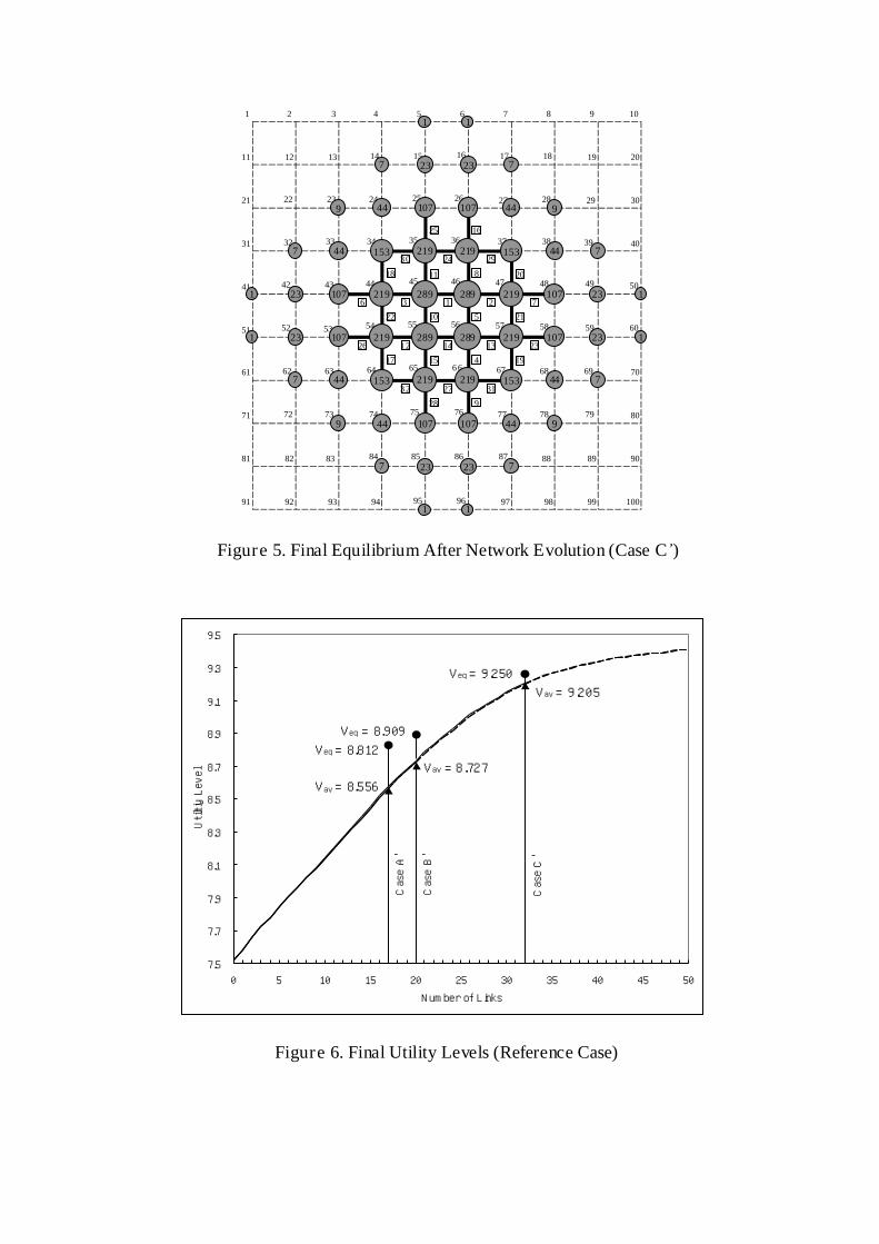
, is taken as 0.5 and the population is moved at five steps with this given migration speed, rather than allowing for instant adjustment. Here, again, cases A', B', and C' correspond to the evolution patterns applying, naive, intermediate, and sophisticated benefit rules, respectively. Figure 5 illustrates the final equilibrium in Case C'. Figure 6 shows the average utility levels right after the termination of the network evolution and the equilibrium utility levels achieved in the long run. For these cases we can easily see that the total number of link improvements is higher than the cases with full equilibrium.

If we compare Figure 6 with Figure 3, we see that the equilibrium utility levels in case of C' follow a flatter path, until the very final link improvement is over. The reason for this is that the system is not necessarily brought into full equilibrium at the end of each period and there is a time lag for the system to adjust itself as a result of the newly formed network structure. After network improvement is terminated at some certain point, the utility levels are still moving towards a long-term equilibrium one. The average and the long-term utility levels are indicated with Vav and Veq in Figure 6. The long-term equilibrium utilities, Veq, are higher than the average utility levels, Vav, for all the cases A', B' and C'. Average utility levels for these three cases seems to follow similar but slightly different paths, just like the equilibrium utility levels in the benchmark cases shown by Figure 3. Comparing the long-term equilibrium levels of cases A', B', and C' with each other, we see that the increase in the equilibrium utility level (regarding that the initial equilibrium utility was 7.521) achieved in case C' is about 24.6% and 33.9% higher than in cases B' and A', respectively. With the existing results we can say that the final network pattern is very sensitive to the values of population adjustment speed. This finding implies that more rigorous cost-benefit evaluations are needed to decide the order of the network link improvements, if the decision maker wishes to contemplate the effects of population adjustment speed on the results of cost-benefit analysis.

5. CONCLUSION

Given the history of network evolution, the cost-benefit evaluation rule guarantees that government will make local optimal decisions. Successive local optimal improvements need not reach the global optimal network. This is especially true if

7.5

7.7

7.9

8.1

8.3

8.5

8.7

8.9

9.1

9.3

9.5

0 5 10 15 20 25 30 35 40 45 50

Number of Links

Utiltiy

Lev

el

Vav = 8.556

Veq = 8.812

Vav = 8.727

Veq = 8.909

Vav = 9.205

Veq = 9.250

Cas

e A

'

Cas

e B

'

Cas

e C

'

1 2 3 4 5 6 7 8 9 10

11 12 13 14 15 16 17 18 19 20

21 22 23 24 25 26 27 28 29 30

31 32 33 34 35 36 37 38 39 40

41 42 43 44 45 46 47 48 49 50

51 52 53 54 55 56 57 58 59 60

61 62 63 64 65 66 67 68 69 70

71 72 73 74 75 76 77 78 79 80

81 82 83 84 85 86 87 88 89 90

91 92 93 94 95 96 97 98 99 100

27

26 13

231314

16

8

5

4

20

21

19

11

10

1512

292430

3132

25

18

17

928

227

26

289

219153

10744

23

9

7

1

289

289 289

219

219 219

219

219

219

219

153

153 153

107

107 107

107

107

107

107

44

44 44

44

44

44

44

23

23 23

23

23

23

23

9

9 9

7

7 7

7

7

7

7

1

1

1 1

1

1

1

Figure 6. Final Utility Levels (Reference Case)

Figure 5. Final Equilibrium After Network Evolution (Case C’)

the city system is inherently characterized by a multiplicity of the equilibria. Even though only a limited number of simulation experiments are presented, we have succeeded in illustrating that the simple succession of cost-benefit evaluation rules may result in highly centralized systems having low efficiency. As far as our simulation experiments are concerned, this becomes even clearer when decisions are made by coarse and naive cost-benefit calculation. It must be noted, however, that it is dangerous to derive a general conclusion based upon a limited number of simulated outcomes. Evolution possibilities with cost-benefit evaluation rules still need further scrutiny from various angles.

The simulation model presented in this paper is a prototype. The model should be improved to conduct more careful investigations. Among others, the following revisions should be made in future research: 1) rebirth of cities that have died along the evolution process should be considered (policy initiatives may lead to the formation of a new city), 2) simultaneous improvement of multiple links during the cost-benefit analysis should be considered, 3) multiple quality ranks allowing for gradual link improvement must be considered, 4) the factors neglected in the model, e.g. knowledge, capital, and trade should be incorporated in the analysis. Growth modeling is the most important direction for further development for changes in the population may inject new equilibrium points and higher inertia and lock- in effects into the existing city system. The issues concerning lock- in effects in the dynamic setting remain unsolved. Although awaiting further development and sophistication, our simulation experiments are encouraging in that they seem to capture the essential mechanism controlling the evolution process of the city systems with cost-benefit evaluation rules.

References

Abdel-Rahman, H.M., 1990, "Agglomeration economies, types, and sizes of cities", Journal of Urban Economics, 27: 25-45.

Alonso, W., 1964, Location and Land Use, Cambridge: Harvard University Press.

Arthur, B., 1994, Increasing Returns and Path Dependence in the Economy, Ann Arbor: The University of Michigan Press.

Batten, D.F., K. Kobayashi and Å.E. Andersson, 1989, "Knowledge, nodes and

networks: an analytical perspective", in: Andersson, Å.E. et al. (eds.), Knowledge and Industrial Organization, Berlin, Heidelberg: Springer Verlag.

Fujita, M., 1993, "Monopolistic competition and urban systems", European Economic Review, 37: 308-315.

Fujita, M, P. Krugman and T. Mori, 1995, "On the evolution of hierarchical urban systems", Discussion Paper 419, Institute of Economic Research, Kyoto University.

Henderson, J. V., 1985, Economic Theory and The Cities, New York: Academic Press.

Hofbauer, J. and K. Sigmund, 1988, The Theory of Evolution and Dynamical Systems, Cambridge: Cambridge University Press.

Kanemoto, Y. and K. Mera, 1985, "General equilibrium analysis of the benefits of large transportation improvements", Regional Science and Urban Economics, 15: 343-363.

Kobayashi, K., D.F. Batten and Å.E. Andersson, 1991, "The sequential location of knowledge-oriented firms over time and space", Paper of Regional Science, 70: 381-397.

Kobayashi, K. and M. Okumura, 1997, "The growth of city systems with high-speed railway systems", Annals of Regional Science, 31: 39-56.

Krugman, P., 1991, "Increasing returns and economic geography", Journal of Political Economy, 99: 483-499.

Lucas, R.E., 1988, "On the mechanics of economic development", Journal of Monetary Economics, 22: 3-22.

Marshall, A., 1920, Principle of Economics, 8th edition, London: Macmillan.

Matsuyama, K., 1995, "Complementarities and cumulative process in models of monopolistic competition", Journal of Economic Literature, 33: 701-729.

Maynard Smith, J., 1982, Evolution and the Theory of Games, Cambridge: Cambridge University Press.

McKibbin, W.J. and J.D. Sachs, 1991, Global Linkages: Macroeconomic Interdependence and Cooperation in the World Economy, Washington, D.C., Brookings Institution.

Mun, S.I., 1997, "Transport network and system of cities", Journal of Urban Economics, 42: 205-221.

Romer, P.M., 1986, "Increasing returns and long-run growth", Journal of Political Economy, 94: 1002-1037.

Sasaki, K., 1992, "Trade and migration in a two-city model of transportation investments", Annals of Regional Science, 26: 305-317.

Smith, J.-M, 1982, Evolution and the Theory of Games, Cambridge: Cambridge University Press.

Shoven, J.B. and J. Whalley, 1992, Applying General Equilibrium, Cambridge: Cambridge University Press.