net foreign assets and the exchange rate: redux...

Journal of Monetary Economics 49 (2002) 1057–1097

Net foreign assets and the exchange rate:Redux revived$

Michele Cavalloa, Fabio Ghironib,*aDepartment of Economics, New York University, New York, NY 10003, USAbDepartment of Economics, Boston College, Chestnut Hill, MA 02467, USA

Received 16 November 2001; received in revised form 5 February 2002; accepted 7 February 2002

Abstract

We revisit Obstfeld and Rogoff’s (1995) results on exchange rate dynamics in a two-country,

monetary model with incomplete asset markets, stationary net foreign assets, and endogenous

monetary policy. The nominal exchange rate exhibits a unit root. Under flexible prices, it also

depends on the stock of real net foreign assets. With sticky prices, the exchange rate depends

on the past GDP differential, along with net foreign assets. Endogenous monetary policy and

asset dynamics have consequences for exchange rate overshooting. A persistent relative

productivity shock results in delayed overshooting under both flexible and sticky prices. A

persistent relative interest rate shock generates undershooting under flexible prices. r 2002

Elsevier Science B.V. All rights reserved.

JEL classification: F31; F32; F41

Keywords: Exchange rate; Monetary policy; Net foreign assets; Overshooting

$We thank Jushan Bai, Jim Bullard, Gabriele Camera, Charles Carlstrom, Mick Devereux, Tim Fuerst,

Philip Lane, Ben McCallum, Fabio Natalucci, Paolo Pesenti, and participants in the November 2001

Carnegie-Rochester Conference on Public Policy and in seminars at Boston College, Dalhousie University,

the Federal Reserve Bank of Cleveland, and Harvard University for helpful conversations and comments.

We are grateful to Kolver Hernandez and Petronilla Nicoletti for excellent research assistance. Remaining

errors are ours. Ghironi thanks IGIER-Bocconi University and the Central Bank Institute of the Federal

Reserve Bank of Cleveland for warm hospitality in the Summer of 2001 and gratefully acknowledges

financial support for this project from Boston College.

*Corresponding author. Tel.: 617-552-3686; fax: 617-552-2308.

E-mail address: [email protected] (F. Ghironi).

0304-3932/02/$ - see front matter r 2002 Elsevier Science B.V. All rights reserved.

PII: S 0 3 0 4 - 3 9 3 2 ( 0 2 ) 0 0 1 2 2 - 8

1. Introduction

Obstfeld and Rogoff’s (1995) ‘‘Exchange Rate Dynamics Redux’’ was originallywritten to put forth a model of exchange rate determination with an explicit role forcurrent account imbalances. The non-stationarity of the model led most of thesubsequent literature in the so-called ‘‘new open economy macroeconomics’’ todevelop in different directions and ‘‘forget’’ the insights of the model on the dynamicrelation between the exchange rate and net foreign asset accumulation by de-emphasizing the role of the latter.1

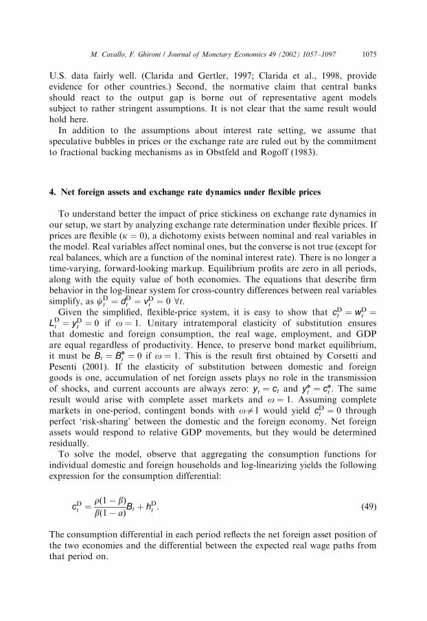
Fig. 1 shows two well known stylized facts: the persistent and growing U.S.current account deficit over the 1990s and the likewise persistent appreciation of thedollar.2 It is a commonly held view that the advent of the ‘‘new economy’’ has beenthe most significant exogenous shock to affect the position of the U.S. economyrelative to the rest of the world in recent years. We can interpret this shock as a(persistent) favorable relative productivity shock. A story that one could tell aboutthe stylized facts in Fig. 1 is that the shock caused the U.S. to borrow from the rest ofthe world and the capital inflow generated exchange rate appreciation. This storycould be reconciled with models of exchange rate determination developed in the1970s and early 1980s. Among others, examples are Dornbusch and Fischer (1980)and Branson and Henderson (1985). If the shock is taken as permanent, the story canalso be reconciled with Obstfeld and Rogoff ’s original model. Nevertheless, the

-400

-350

-300

-250

-200

-150

-100

-50

0

50

100

Q 1

/199

0

Q 4

/199

0

Q 3

/199

1

Q 2

/199

2

Q 1

/199

3

Q 4

/199

3

Q 3

/199

4

Q 2

/199

5

Q 1

/199

6

Q 4

/199

6

Q 3

/199

7

Q 2

/199

8

Q 1

/199

9

Q 4

/199

9

60

70

80

90

100

110

120

130

Current account Dollar effective exchange rate

Fig. 1. The dollar and the U.S. current account.

1This is achieved either by assuming unitary intratemporal elasticity of substitution between domestic

and foreign goods in consumption as in Corsetti and Pesenti (2001) or by combining the assumptions of

complete markets and power utility. Kollmann (2001) is a recent exception to the trend, although he uses a

non-stationary model. For a survey of the literature, see Lane (2001).2Source: National Accounts and Federal Reserve, respectively. Effective dollar rate: Broad exchange

rate weighted average. Current account unit: billions of dollars.

M. Cavallo, F. Ghironi / Journal of Monetary Economics 49 (2002) 1057–10971058

argument cannot be reconciled with the overwhelming majority of new generationmodels that followed.

In this paper, we go back to the original intent of Obstfeld and Rogoff’s work anddevelop a two-country model of exchange rate determination in which stationary netforeign asset dynamics play an explicit role. We deal with indeterminacy of the steadystate and non-stationarity of the original incomplete markets setup by adopting theoverlapping generations framework illustrated in Ghironi (2000). If exogenous shocksare stationary, the departure from Ricardian equivalence generated by the birth ofnew households with no assets in all periods is sufficient to ensure existence of adeterminate steady state and stationarity of real variables. Unexpected temporaryshocks cause countries to run current account imbalances, which are re-absorbedover time as the world economy returns to the original steady state.3

Differently from Obstfeld and Rogoff (1995) (and in line with the more recentliterature on monetary policy), we allow for endogenous monetary policy in the formof interest rate reaction functions for the two countries. We consider familiar interestsetting rules as in Taylor (1993). Interest rates react to the deviations of CPI inflationand GDP from their steady-state levels. They are also subject to exogenous shocks toallow for the possibility of exogenous changes in monetary policy.4

We solve the model with the method of undetermined coefficients illustrated inCampbell (1994). We rely on Uhlig’s (1999) implementation of the method whensolving the model numerically. The method has the advantage of delivering a processequation for the exchange rate with straightforward quantitative and empiricalimplications.

We are able to solve a benchmark model with purchasing power parity and flexibleprices analytically. The solution for the nominal exchange rate exhibits a unit root,consistent with the empirical findings of Meese and Rogoff (1983). However, today’sexchange rate also depends on the stock of real net foreign assets accumulated in theprevious period. The intuition is as follows. No-arbitrage ensures that uncoveredinterest parity holds in our model: expected exchange rate depreciation equals thenominal interest rate differential. To the extent that interest rates react to variablesthat are affected by net foreign assets (namely, GDP, through the wealth effect onlabor supply), net foreign assets affect the exchange rate too. Thus, the model impliesthat asset holdings help predict the nominal exchange rate. Consistent with theevidence for the U.S., ceteris paribus, a decrease in asset holdings—a current account

3Alternative approaches to the non-stationarity issue that preserve a role for net foreign asset dynamics

under incomplete markets rely on introducing a cost of bond holdings, an endogenous discount factor, or

a debt-sensitive risk premium. See Ghironi (2000) and Schmitt-Groh!e and Uribe (2001) for references and

discussion. (Schmitt-Groh!e and Uribe compare the quantitative performance of these approaches in a

small open economy setup.) Net foreign asset dynamics do not hinge on assumptions about a bond

holding cost function or a non-standard discount factor in our model. Each individual household in the

economy behaves as the representative agent of the original Obstfeld-Rogoff setup. Aggregate per capita

assets are stationary, individual household’s are not. Devereux (2002) and Smets and Wouters (2002) are

recent studies that use a setup similar to ours.4Benigno and Benigno (2001) study the consequences of endogenous interest setting for exchange rate

dynamics in a sticky-price model with no net foreign asset accumulation.

M. Cavallo, F. Ghironi / Journal of Monetary Economics 49 (2002) 1057–1097 1059

deficit/capital inflow—generates an appreciation of the domestic currency forreasonable parameter values. The response of the exchange rate to shocks is moredifferent from that of a simple random walk the slower the convergence of netforeign assets to the steady state and the higher the degree of substitutability betweendomestic and foreign goods in consumption.

The exchange rate overshoots its new long-run level following a temporary(relative) productivity shock. If the shock is persistent, endogenous monetary policyand asset dynamics generate delayed overshooting. Endogenous monetary policy isresponsible for exchange rate undershooting after persistent (relative) interest rateshocks. (‘‘Persistent’’ does not mean ‘‘permanent’’ throughout the paper. When weconsider permanent shocks, we say so explicitly.)

Next, we analyze exchange rate and asset dynamics in a sticky-price world. Weintroduce price stickiness by assuming that it is costly to change output prices overtime as in Rotemberg (1982). It is harder to solve the model analytically in this case.We investigate the effect of nominal and real shocks using a plausible calibration ofthe model. When prices are sticky, the exchange rate still exhibits a unit root underthe Taylor rule, as in Benigno and Benigno (2001). The current level of the exchangerate depends on the past GDP differential, along with net foreign assets. Temporaryshocks to relative productivity result in delayed overshooting. So do persistentshocks. Temporary relative interest rate shocks cause immediate overshooting. Noovershooting may happen when interest rate shocks are persistent.

Our results on exchange rate overshooting contrast with Obstfeld and Rogoff’s(1995), who obtain no overshooting following monetary and/or productivity shocksin their benchmark setup. We show that price stickiness is not necessary to generateovershooting once asset dynamics and endogenous monetary policy are accountedfor. This brings a new perspective to bear on a topic that has been at the center oftheoretical and empirical research on exchange rates since Dornbusch’s (1976)seminal paper. Our model has the potential for reconciling the evidence in favor ofdelayed overshooting in Clarida and Gal!ı (1994) and Eichenbaum and Evans (1995)with rational behavior and uncovered interest parity.

As far as the empirical performance is concerned, the model delivers exchange rateappreciation following a favorable shock to relative productivity in an environmentin which monetary policy follows the Taylor rule. However, the model does notgenerate accumulation of net foreign debt following the shock, unless the latter ispermanent and prices are sticky. The reason is that consumption smoothing is theonly motive for asset accumulation in the model. If the relative productivity shock ispermanent and prices are sticky, the new long-run level of domestic GDP relative toforeign is above the short-run differential, which causes domestic agents to borrowfrom abroad to smooth consumption. It remains to be seen whether the advent of the‘‘new economy’’ has shifted U.S. productivity permanently above foreign. If onebelieves that the shock has been persistent, but not permanent, the model can explainonly part of the dynamics in Fig. 1. Inclusion of capital accumulation andinvestment appears a promising way of completing the theory. On more rigorousgrounds, the model yields straightforward, empirically testable implications forexchange rate dynamics.


The rest of the paper is organized as follows. Section 2 presents the model. Section3 illustrates the log-linear equations that determine exchange rate and assetdynamics. Section 4 discusses the relation between net foreign assets and theexchange rate under flexible prices. Section 5 extends the analysis to the case of stickyprices. Section 6 concludes.

2. The model

The model is a monetary version of the setup in Ghironi (2000). The worldconsists of two countries, home and foreign. In each period t; the world economy ispopulated by a continuum of infinitely lived households between 0 and NW

t : Eachhousehold consumes, supplies labor, and holds financial assets. As in Weil (1989), weassume that households are born on different dates owning no assets, but they ownthe present discounted value of their labor income.5 The number of households inthe home economy, Nt; grows over time at the exogenous rate n > 0; i.e., Ntþ1 ¼ð1þ nÞNt: We normalize the size of a household to 1, so that the number ofhouseholds alive at each point in time is the economy’s population. Foreignpopulation ðNn

t Þ grows at the same rate as home population. The world economy hasexisted since the infinite past. It is useful to normalize world population at time 0 tothe continuum between 0 and 1, so that NW

0 ¼ 1:A continuum of goods iA½0; 1� are produced in the world by monopolistically

competitive, infinitely lived firms, each producing a single differentiated good. Firmshave existed since the infinite past. At time 0, the number of goods that are suppliedin the world economy is equal to the number of households. The latter grows overtime, but the commodity space remains unchanged. Thus, as time goes, theownership of firms spreads across a larger number of households. Profits aredistributed to consumers via dividends, and the structure of the market for eachgood is taken as given. We assume that the domestic economy produces goods in theinterval ½0; a�; which is also the size of the home population at time 0; whereas theforeign economy produces goods in the range ða; 1�:

The asset menu includes nominal, uncontingent bonds denominated in units ofdomestic and foreign currency, money balances, and shares in firms. Private agentsin both countries trade the bonds domestically and internationally. Shares in home(foreign) firms and domestic (foreign) currency balances are held only by home(foreign) residents.

2.1. Households

Agents have perfect foresight, though they can be surprised by initial unexpectedshocks. Consumers have identical preferences over a real consumption index ðCÞ;

5Blanchard (1985) combines this assumption with a positive probability of not surviving until the next

period. This is advantageous for calibration purposes (see below), besides being plausible. We adopt the

Weil setup here because it is relatively simpler to illustrate.


labor effort supplied in a competitive market ðLÞ; and real money balances (M=P;where M denotes nominal money holdings and P is the consumption-based priceindex—CPI). We normalize the endowment of time in each period to 1: At any timet0; the representative home consumer j born in period uA½�N; t0� maximizes theintertemporal utility function:

U ujt0¼

XNt¼t0

bt�t0 r logCujt þ ð1� rÞlogð1� Luj

t Þ þ w logMuj

t

Pt

" #; ð1Þ

with 0oro1:6

The consumption index for the representative domestic consumer is a standardCES aggregator of foreign and domestic sub-indexes:

Cujt ¼ ½a1=oðCuj

HtÞðo�1Þ=o þ ð1� aÞ1=oðCuj

FtÞðo�1Þ=o�o=ðo�1Þ;

where o > 0 is the intratemporal elasticity of substitution between domestic andforeign goods. The consumption sub-indexes that aggregate individual domestic andforeign goods are, respectively,

CujHt ¼

1

a

� �1=yZ a

0

cuj

t ðiÞðy�1Þ=y di

" #y=ðy�1Þ

and

CujFt ¼

1

1� a

� �1=yZ 1

a

cuj

ntðiÞðy�1Þ=y di

" #y=ðy�1Þ

;

where cuj

ntðiÞ denotes time t consumption of good i produced in the foreign country,and y > 1 is the elasticity of substitution between goods produced inside eachcountry.

The CPI is Pt ¼ ½aP1�oHt þ ð1� aÞP1�o

Ft �1=ð1�oÞ; where PH (PF) is the price sub-indexfor home (foreign)-produced goods—both expressed in units of the home currency.Letting ptðiÞ be the home currency price of good i; we have PHt ¼ð1a

R a

0 ptðiÞ1�y diÞ1=ð1�yÞ and PFt ¼ ð 1

1�a

R 1

aptðiÞ

1�y diÞ1=ð1�yÞ:We assume that there are no impediments to trade and that firms do not engage in

local currency pricing (i.e., pricing in the currency of the economy where goods aresold). Hence, the law of one price holds for each individual good and ptðiÞ ¼ etpnt ðiÞ;where et is the exchange rate (units of domestic currency per unit of foreign) and pnt ðiÞis the foreign currency price of good i: This hypothesis and identical intratemporalconsumer preferences across countries ensure that consumption-based purchasingpower parity (PPP) holds, i.e., Pt ¼ etPn

t :

6We focus on domestic households. Foreign agents maximize an identical utility function. They

consume the same basket of goods as home agents, with identical parameters, and they are subject to

similar constraints. We will sometimes refer to the representative consumer of generation u simply as the

‘‘representative consumer’’ below. It is understood that consumers of different generations can behave

differently in our model.


The representative consumer enters a period holding bonds, money balances, andshares purchased in the previous period. She or he receives interests and dividends onthese assets, may earn capital gains or incur losses on shares, earns labor income, istaxed, and consumes.

Denote the date t price (in units of domestic currency) of a claim to therepresentative domestic firm i’s entire future profits (starting on date tþ 1) by Vi

t :Let xu

ji

tþ1 be the share of the representative domestic firm i owned by therepresentative domestic consumer j born in period u at the end of period t: Di

t

denotes the nominal dividends firm i issues on date t: Then, letting Aujtþ1ðA

nujtþ1Þ be the

home consumer’s holdings of domestic (foreign) currency denominated bondsentering time tþ 1; the period budget constraint expressed in units of domesticcurrency is:

PtCujt þ PtT

ut þ Auj

tþ1 þ etAnujtþ1 þ

Z a

0

Vitx

ujitþ1 di þMuj

t

¼ ð1þ itÞAujt þ etð1þ int ÞA

nujt þ

Z a

0

ðVit þDi

tÞxujit di þMuj

t�1 þWtLujt ; ð2Þ

where it (int ) is the nominal interest rate on holdings of domestic (foreign) bonds

between t� 1 and t; Wt is the nominal wage, Mujt�1 denotes the agent’s holdings of

nominal money balances entering period t; and T ut is a lump-sum net real transfer,

which is identical across members of generation u: Given that individuals are bornowning no financial wealth, because not linked by altruism to individuals born inprevious periods, Auj

u ¼ Anuju ¼ xu

ji

u ¼ Muju�1 ¼ 0:

The representative domestic consumer born in period u maximizes theintertemporal utility function (1) subject to the constraint (2). Dropping the j

superscript (because symmetric agents make identical choices in equilibrium),optimal labor supply is given by:

Lut ¼ 1�

1� rr

Cut

wt

; ð3Þ

which equates the marginal cost of supplying labor with the marginal utility ofconsumption generated by the corresponding increase in labor income (wt denotesthe real wage, Wt=Pt).

Making use of this equation, the first-order condition for optimal holdings ofdomestic currency bonds yields the Euler equation:

Cut ¼ bð1þ itþ1Þ

Pt

Ptþ1

� �� 1

Cutþ1 ð4Þ

for all upt:Demand for home currency real balances is:

Mut

Pt

¼wr1þ itþ1

itþ1Cu

t : ð5Þ

Real domestic currency balances increase with consumption and decrease with theopportunity cost of holding money.


Condition (4) can be combined with the first-order condition for holdings offoreign bonds to yield a no-arbitrage condition between domestic and foreigncurrency bonds for domestic agents. Absence of unexploited arbitrage opportunitiesrequires:

1þ itþ1 ¼ ð1þ intþ1Þetþ1

et: ð6Þ

The consumption-based real interest rate between t and tþ 1 is defined by thefamiliar Fisher parity condition

1þ rtþ1 ¼ ð1þ itþ1ÞPt

Ptþ1¼

1þ itþ1

1þ pCPItþ1

; ð7Þ

where pCPItþ1 is CPI inflation ðpCPItþ1 � ðPtþ1=PtÞ � 1Þ: PPP ensures that 1þ pCPIt ¼ð1þ etÞð1þ pCPI

n

t Þ; where 1þ pCPIn

t � Pnt =P

nt�1 and 1þ et � et=et�1: Combining (7)

with (6) and making use of PPP shows that 1þ rtþ1 ¼ 1þ rntþ1 ¼ ð1þ intþ1ÞPnt =P

ntþ1:

real interest rates are equal across countries in the absence of unexpected shocks thatmay cause no-arbitrage conditions to fail ex post.

Absence of arbitrage opportunities between bonds and shares in the domesticeconomy requires 1þ itþ1 ¼ ðDi

tþ1 þ Vitþ1Þ=V

it : Letting di

t � Dit=Pt and vit ¼ Vi

t=Pt;we can re-write this no-arbitrage condition as

1þ rtþ1 ¼ditþ1 þ vitþ1

vit: ð8Þ

As usual, first-order conditions and the period budget constraint must becombined with appropriate transversality conditions to ensure optimality.

2.2. Firms

Output supplied at time t by the representative domestic firm i is a linear functionof labor demanded by the firm:

Y Sit ¼ ZtL

it: ð9Þ

Zt is an exogenous economy-wide productivity parameter. Production by therepresentative foreign firm is a linear function of Lin

t ; with productivity para-meter Zn

t :7

Output demand comes from several sources: domestic and foreign consumers anddomestic and foreign firms. The demand for home good i by the representative homeconsumer born in period u is cut ðiÞ ¼ ðptðiÞ=PHtÞ

�yðPHt=PtÞ�oCu

t ; obtained bymaximizing Cu subject to a spending constraint. Total demand for home good i

7Because all firms in the world economy are born at t ¼ �N; after which no new goods appear, it is not

necessary to index output and factor demands by the firms’ date of birth. As for consumers, we focus on

domestic firms below. Foreign firms are symmetric in all respects.


coming from domestic consumers is

ctðiÞ ¼ ay

nð1þnÞtþ1 c

�tt ðiÞ þ?þ n

ð1þnÞ2c�1t ðiÞ þ n

1þnc0t ðiÞ

þnc1t ðiÞ þ nð1þ nÞc2t ðiÞ þ?þ nð1þ nÞt�1cttðiÞ

" #

¼ptðiÞPHt

� ��yPHt

Pt

� ��o

að1þ nÞtct; ð10Þ

where

ct �

ay

nð1þnÞtþ1 C

�tt þ?þ n

ð1þnÞ2C�1

t þ n1þn

C0t

þnC1t þ nð1þ nÞC2

t þ?þ nð1þ nÞt�1Ctt

" #

að1þ nÞtð11Þ

is aggregate per capita home consumption.Given identity of intratemporal preferences, total demand for the same good by

foreign consumers is cnt ðiÞ ¼ ðptðiÞ=PHtÞ�yðPHt=PtÞ

�oð1� aÞð1þ nÞtcnt ; where cnt isaggregate per capita foreign consumption.

Changing the price of its output is costly for the firm, which generates nominalrigidity. Specifically, we assume that the real cost (measured in units of the compositegood) of output-price inflation volatility around a steady-state level of inflationequal to 0; is PACi

t � ðk=2Þ½ðptðiÞ=pt�1ðiÞÞ � 1�2ðptðiÞ=PtÞYit : When the firm changes

the price of its output, a set of material goods—e.g., new catalogs, price tags, etc.—need to be purchased. The price adjustment cost (PACi) captures the amount ofmarketing materials that must be purchased to implement a price change. Becausethe amount of these materials is likely to increase with firm size, PACi increases withrevenues ððptðiÞ=PtÞYi

t Þ; which are taken as a proxy for size. The cost is convex ininflation; faster price movements are more costly to the firm. We assume kX0: Whenk ¼ 0; prices are flexible. The quadratic specification for the cost of adjusting prices,first introduced by Rotemberg (1982), yields dynamics for the aggregate economythat are similar to those resulting from staggered price setting as in Calvo (1983).

Total demand for good i produced in the home country is obtained by adding thedemands for that good originating in the two countries. Making use of the resultsabove, it is

YDit ¼

ptðiÞPHt

� ��yPHt

Pt

� ��o

YDWt : ð12Þ

YDWt is aggregate world demand of the composite good, defined as YDW

t �CW

t þ PACWt : CW

t � ð1þ nÞt½act þ ð1� aÞcnt � and PACWt � aPACi

t þ ð1� aÞPACnit

denote aggregate world consumption and the world aggregate cost of adjustingprices, respectively.8

8The expression for the world aggregate cost of adjusting prices derives from the assumption that the

number of firms is constant. In the expression for PACWt ; we have already made use of the fact that

symmetric firms make identical equilibrium choices. Keeping the i superscript for individual firms’

variables allows us to denote several aggregate per capita variables referring to firms by dropping the

superscript below.


At time t0; firm i maximizes the present discounted value of dividends to be paidfrom t0 on: vit0 þ di

t0¼

PN

s¼t0Rt0;sd

is; where

Rt0;s �1Qs

u¼t0þ1ð1þ ruÞ; Rt0;t0 ¼ 1:

Firm revenues are taxed at a constant, proportional rate t: In addition, firms receivea lump-sum transfer (or tax) from the government, T

fit : At each point in time,

dividends are given by real revenues, net of taxes, plus the lump-sum transfer,minus costs: di

t ¼ ð1� tÞðptðiÞ=PtÞYit þ T

fit � fðWt=PtÞLi

t þ ðk=2Þ½ðptðiÞ=pt�1ðiÞÞ �1�2ðptðiÞ=PtÞYi

tg: The firm chooses the price of its product and the amount of labordemanded in order to maximize the present discounted value of its current andfuture profits subject to constraints (9) and (12), and the market clearing conditionYi

t ¼ Y Sit ¼ YDi

t : Firm i takes the aggregate price indexes, the wage rate, Zt; worldaggregates, and taxes and transfers as given.

Let lit denote the Lagrange multiplier on the constraint Y Sit ¼ YDi

t : Then, lit is theshadow price of an extra unit of output to be sold in period t; or the marginal cost oftime t sales. The first-order condition with respect to ptðiÞ yields the pricing equation:

PtðiÞ ¼ CitPtl

it; ð13Þ

which equates the price charged by firm i to the product of the (nominal) shadow valueof one extra unit of output—the (nominal) marginal cost ðPtl

itÞ—and a markup (Ci

t).The latter depends on output demand as well as on the impact of today’s pricingdecision on today’s and tomorrow’s costs of adjusting the output price:

Cit � yYi

t ðy� 1ÞYit 1� t�

k2

ptðiÞpt�1ðiÞ

� 1

� �2" #

þ kU it

( )�1

; ð14Þ

where

U it � Yi

t

ptðiÞpt�1ðiÞ

ptðiÞpt�1ðiÞ

� 1

� ��

Yitþ1

1þ rtþ1

Pt

Ptþ1

ptþ1ðiÞptðiÞ

� �2ptþ1ðiÞptðiÞ

� 1

� �

reflects the firm’s incentive to smooth price changes over time.If k ¼ 0; i.e., if prices are fully flexible, Ci

t ¼ y=½ðy� 1Þð1� tÞ�; the familiarconstant-elasticity markup. If ka0; price rigidity generates endogenous fluctuationsof the markup. Firms react to CPI dynamics in their pricing decisions. Changes inmonetary policy generate changes in CPI inflation. Hence, they affect producerprices and the markup. Through this channel, they generate different dynamics ofrelative prices and the real economy.

The first-order condition for the optimal choice of Lit yields

Wt

Pt

¼ litZt: ð15Þ

Today’s real wage must equal the shadow value of an extra unit of labor inproduction.

Using the market clearing conditions Y Sit ¼ YDi

t and YDWt ¼ YSW

t ¼ YWt ; the

expressions for supply and demand of good i; and recalling that symmetric firms


make identical equilibrium choices (so that ptðiÞ ¼ PHt and ptðiÞ is the producer priceindex, PPI) yields

Lit ¼

ptðiÞPt

� ��oYW

t

Zt

: ð16Þ

Firm i’s labor demand is a decreasing function of the relative price of good i and oflabor productivity. It is an increasing function of world demand of the compositegood. Henceforth, we denote the relative price of good i by RPi

t � ptðiÞ=Pt:

2.3. The government

We assume that governments in both countries run balanced budgets. Thegovernment taxes firm revenues at a rate that compensates for monopoly power in azero-inflation steady state and removes the markup over marginal cost charged byfirms in a flexible-price world. The tax rate is determined by 1� t ¼ y=ðy� 1Þ; whichyields t ¼ �1=ðy� 1Þ: Because the tax rate is negative, firms receive a subsidy ontheir revenues and pay lump-sum taxes determined by T

fit ¼ tRPi

tYit : In addition, the

government injects money into the economy through lump-sum transfers ofseignorage revenues to households: PtT

ut ¼ �ðMuj

t �Mujt�1Þ: Similarly for the foreign

government.

2.4. Aggregation and equilibrium

2.4.1. Households

Aggregate per capita consumption and labor supply are obtained by aggregatingconsumption and labor supply across generations and dividing by total populationat each point in time. Aggregate per capita labor supplies follow from aggregatingthe labor–leisure tradeoffs in the two economies

Lt ¼ 1�1� rr

ct

wt

; Ln

t ¼ 1�1� rr

cntwnt

: ð17Þ

Labor supply rises with the real wage and decreases with consumption.Consumption Euler equations in aggregate per capita terms contain an adjustment

for consumption by the newborn generation at time tþ 1:

ct ¼1þ n

bð1þ rtþ1Þctþ1 �

n

1þ nCtþ1

tþ1

� �;

cnt ¼1þ n

bð1þ rtþ1Þcntþ1 �

n

1þ nCtþ1n

tþ1

� �:

ð18Þ

Newborn households hold no assets, but they own the present discounted value oftheir labor income. We define human wealth, ht; as the present discounted value ofthe household’s lifetime endowment of time in terms of the real wage: ht �P

N

s¼t Rt;sws; hnt �P

N

s¼t Rt;swns : The dynamics of h and hn are described by the


following forward-looking difference equations:

ht ¼htþ1

1þ rtþ1þ wt; hnt ¼

hntþ1

1þ rtþ1þ wn

t : ð19Þ

Using the labor–leisure tradeoff (3), the Euler equation (4), and a newbornhousehold’s intertemporal budget constraint, it is possible to show that thehousehold’s consumption in the first period of its life is a fraction of the household’shuman wealth at birth:

Ctþ1tþ1 ¼ rð1� bÞhtþ1; Ctþ1n

tþ1 ¼ rð1� bÞhntþ1: ð20Þ

Aggregate per capita real money demands in the two economies are:

mt �Mt

Pt

¼wr1þ itþ1

itþ1ct; mn

t �Mn

t

Pnt

¼wr1þ intþ1

intþ1

cnt : ð21Þ

In the absence of arbitrage opportunities between bonds and shares, the aggregateper capita equity values of the home and foreign economies entering period tþ 1must evolve according to:

vt ¼1þ n

1þ rtþ1vtþ1 þ

dtþ1

1þ rtþ1; vnt ¼

1þ n

1þ rtþ1vntþ1 þ

dntþ1

1þ rtþ1: ð22Þ

where vt � aVit=ðPtNtþ1Þ; vnt � aVni

t =ðPnt N

ntþ1Þ; and dt and dn

t denote aggregate percapita real dividends, equal to ð1� tÞyt þ T

ft � wtLt � pact and ð1� tnÞynt þ T

f nt �

wnt L

nt � pacnt ; respectively (note that t ¼ tn). yt (ynt ) denotes domestic (foreign)

aggregate per capita, real GDP, defined below. pact (pacnt ) is the aggregate per capita

cost of nominal rigidity at home (abroad).The law of motion of aggregate per capita net foreign assets is obtained by

aggregating an equilibrium version of the budget constraint (2) across generationsalive at each point in time. It is:

ð1þ nÞBtþ1 ¼ ð1þ rtÞBt þ wtLt þ dt � ct;

ð1þ nÞBntþ1 ¼ ð1þ rtÞBn

t þ wnt L

nt þ dn

t � cnt ;ð23Þ

where

Btþ1 �Atþ1 þ etAn

tþ1

Pt

and Bn

tþ1 �Antþ1

etþ An

ntþ1

Pnt

denote domestic and foreign net bond holdings (An denotes foreign households’holdings of home bonds, An

ndenotes their holdings of foreign bonds). A country’s

net foreign assets and net foreign bond holdings coincide in a world in which allshares are held domestically.9

9Strictly speaking, these equations hold in all periods after the initial one. No-arbitrage conditions may

be violated between time t0 � 1 and t0 if an unexpected shock surprises agents at the beginning of period t0:Using log-linear versions of these equations to determine asset accumulation in the initial period is

harmless if one is willing to assume that the steady-state levels of A; An; An; and Annare all zero. (As we

show below, the model pins down the steady-state levels of B and Bn endogenously. Because domestic and

foreign bonds are perfect substitutes once no-arbitrage conditions are met, the model does not pin down

the levels of A; An; An; and Ann:)


Because dt ¼ yt � wtLt � pact and dnt ¼ ynt � wn

t Lnt � pacnt in equilibrium, the

equations in (23) become

ð1þ nÞBtþ1 ¼ ð1þ rtÞBt þ yt � ct � pact;

ð1þ nÞBntþ1 ¼ ð1þ rtÞBn

t þ ynt � cnt � pacnt :ð24Þ

2.4.2. Firms

Aggregate per capita, real GDP in each economy is obtained by expressingproduction of each differentiated good in units of the composite basket, multiplyingby the number of firms, and dividing by population. In equilibrium, RPi

t ¼ RPt andsimilarly for foreign firms. Thus:

yt ¼ RPtZtLt; ynt ¼ RPn

t Zn

t Ln

t : ð25Þ

For given employment and productivity, real GDP rises with the relative price of therepresentative good produced, as this is worth more units of the consumption basket.

Aggregate per capita labor demand is:

Lt ¼ RP�ot

yWtZt

; Ln

t ¼ RPn�o

t

yWtZn

t

; ð26Þ

where yWt is aggregate per capita world production of the composite good, equal toaggregate per capita world consumption plus the aggregate per capita resource costof price changes, cWt þ pacWt : It is yWt ¼ ayt þ ð1� aÞynt ; cWt ¼ act þ ð1� aÞcnt ;pacWt ¼ apact þ ð1� aÞpacnt : Market clearing requires yWt ¼ cWt þ pacWt :

Domestic and foreign relative prices are equal to markups over marginal costs:

RPt ¼ Ct

wt

Zt

; RPn

t ¼ Cn

t

wnt

Znt

: ð27Þ

2.4.3. International equilibrium

For international asset markets to be in equilibrium, net, aggregate home assets(liabilities) must equal net, aggregate foreign liabilities (assets). In terms ofaggregates per capita, it must be aBt þ ð1� aÞBn

t ¼ 0: Using this condition, theequations in (24) reduce to yWt ¼ cWt þ pacWt : consistent with Walras’ Law, assetmarket equilibrium implies goods market equilibrium, and vice versa.

2.5. The steady state

2.5.1. Real variables

The procedure for finding the steady-state levels of real variables follows the samesteps as in Ghironi (2000). As described there, the departure from Ricardianequivalence caused by entry of new households with no assets in each period generatesdependence of aggregate per capita consumption growth on the stock of aggregate percapita net foreign assets. This yields determinacy of steady-state real net foreign assetholdings, and thus of the steady-state levels of other real variables in the model.

We denote steady-state levels of variables with overbars. A subscript �1 indicatesthat the steady state described below is going to be the position of the economy up to


and including period t ¼ �1 in our exercise.10 Unexpected shocks can surprise agentsat the beginning of period 0, generating the dynamics we describe in the followingsections.

Given initial steady-state levels of productivity ð %Z�1 ¼ %Zn�1 ¼ 1Þ and inflation

ð %pPPI�1 ¼ %pPPIn

�1 ¼ %pCPI�1 ¼ %pCPIn

�1 ¼ 0; where pPPIt � ðptðiÞ � pt�1ðiÞÞ=pt�1ðiÞ and pPPIn

t isdefined similarly), real variables are stationary, in the sense that they return to theinitial position determined below following non-permanent shocks to productivityand/or inflation. (The restriction that inflation shocks ought not to be permanent forreal variables to return to the steady state described below applies to the general casein which prices are sticky (k > 0). If prices are flexible (k ¼ 0), real variables return tothe steady state below also after permanent changes in inflation. When k > 0;permanent deviations of domestic or foreign inflation from zero impose permanentresource costs on the economy. These costs generate a different long-run equilibriumfor real variables.)

The model determines the steady state as follows. Consider the home economy,and set aggregate per capita consumption to be constant. It is:

%c�1 1�bð1þ %r�1Þ

1þ n

� �¼

n

1þ n%Cuu�1

;

where %Cuu is steady-state consumption by a newborn generation in the first period of

its life. It must be bð1þ %r�1Þ=ð1þ nÞo1 for steady-state consumption to be positive.As we shall see, this holds as long as n > 0: Now, from Eq. (20) and the definition ofh; it is %Cu

u�1¼ rð1� bÞ½ð1þ %r�1Þ=%r�1� %w�1: Hence, aggregate per capita consumption

as a function of the steady-state interest rate and real wage is

%c�1 ¼nrð1� bÞð1þ %r�1Þ

%r�1½1þ n� bð1þ %r�1Þ�%w�1: ð28Þ

Under the assumption that %Z�1 ¼ 1; steady-state GDP is %y�1 ¼ RP�1 %L�1: Fromthe pricing equation, RP�1 ¼ %w�1; because the monopolistic distortion is removedby the subsidy t: It follows that

%y�1 ¼ %w�1 %L�1: ð29Þ

Using Eqs. (28), (29), and steady-state versions of the domestic labor supply in(17) and of the law of motion for home’s net foreign assets yields

%B0 ¼1

%r�1 � n

nð1� bÞð1þ %r�1Þ � %r�1½1þ n� bð1þ %r�1Þ�%r�1½1þ n� bð1þ %r�1Þ�

� �%w�1: ð30Þ

The subscript for initial steady-state asset holdings is 0 rather than �1 because time-0 asset holdings are determined at time �1: Foreign steady-state assets ð %Bn

0Þ are givenby a similar expression, function of %r�1 and %wn

�1: Substituting for %B0 and %Bn0 in the

asset market equilibrium condition, a %B0 þ ð1� aÞ %Bn0 ¼ 0; yields

10There are two reasons for time indexes for steady-state levels of variables. On one side, when we

consider non-stationary exogenous shocks, these will cause the economy to settle at a new long-run

position. On the other side, we shall see that the levels of nominal variables may exhibit a unit root

regardless of stationarity of the exogenous shocks.


1

%r�1 � n

nð1� bÞð1þ %r�1Þ � %r�1½1þ n� bð1þ %r�1Þ�%r�1½1þ n� bð1þ %r�1Þ�

� �� ½a %w�1 þ ð1� aÞ %wn

�1� ¼ 0: ð31Þ

Given non-zero real wages at home and abroad, the only admissible level of theinterest rate that satisfies the market clearing condition is such that bð1þ %r�1Þ ¼ 1;or %r�1 ¼ ð1� bÞ=b: Substituting this result into the expressions for %B0 and %Bn

0 yieldssteady-state levels of domestic and foreign net foreign assets %B0 ¼ %Bn

0 ¼ 0: Consistentwith the fact that the two economies are structurally symmetric in per capita terms,the long-run net foreign asset position is a zero equilibrium. Differently fromObstfeld and Rogoff (1995), this position is pinned down endogenously by the model.

Given these results, it is easy to verify that steady-state levels of endogenousvariables other than real balances are:

%w�1 ¼ RP�1 ¼ %wn

�1 ¼ RPn

�1 ¼ 1; %h�1 ¼ %hn�1 ¼1

1� b;

%y�1 ¼ %c�1 ¼ %Cuu�1

¼ %L�1 ¼ %yn�1 ¼ %cn�1 ¼ %Cunu�1

¼ %Ln

�1 ¼ %yW�1 ¼ %cW�1 ¼ r;

%C�1 ¼ %Cn

�1 ¼ 1; pac�1 ¼ %d�1 ¼ %v�1 ¼ pacn�1 ¼ %dn�1 ¼ %vn

�1 ¼ 0:

2.5.2. Real money balances and nominal variables

Given steady-state consumption, domestic steady-state real balances aredetermined by %m�1 ¼ wð1þ %i�1Þ=ð%i�1Þ: Similarly for foreign. In a zero-inflationsteady state, nominal interest rates at home and abroad are equal to the steady-statereal interest rate: %i�1 ¼ %in�1 ¼ ð1� bÞ=b: It follows that domestic and foreign realbalances are, respectively: %m�1 ¼ %mn

�1 ¼w

1�b:Nominal money balances at home and abroad are determined by, respectively:

%M�1 ¼ ½w=ð1� bÞ� %P�1; %Mn�1 ¼ ½w=ð1� bÞ� %Pn

�1: Taking the ratio of %M�1 to %Mn�1 and

using PPP yields %e�1 ¼ %M�1= %Mn�1: The steady-state exchange rate equals the

ratio of money supplies. In the analysis below, we assume that monetary policy isconducted by setting the nominal interest rate. In order to pin down the initialsteady-state level of the exchange rate, we assume that the initial level of moneysupplies was set by the domestic and foreign central banks at %M�1 ¼ %Mn

�1 ¼w=ð1� bÞ: Structural symmetry of the two economies implies that the centralbanks’ optimal choice of steady-state money supplies would satisfy %M�1 ¼ %Mn

�1 ifthe two authorities had identical objectives. The level w=ð1� bÞ conveniently implies

%e�1 ¼ %P�1 ¼ %Pn�1 ¼ %p�1ðhÞ ¼ %pn�1ð f Þ ¼ 1 ( %p�1ðhÞ and %pn�1ð f Þ are the steady-state

levels of the domestic and foreign PPIs, respectively, which follow fromRP�1 ¼ %p�1ðhÞ= %P�1 ¼ RP

n

�1 ¼ %pn�1ð f Þ= %Pn�1 ¼ 1). The model does not pin down the

steady-state levels of all nominal variables endogenously as functions of thestructural parameters only. As a consequence, monetary policy may generatethe presence of a unit root in the dynamics of price levels, the exchange rate, andnominal money balances. Steady-state levels of nominal variables may change as aconsequence of temporary shocks depending on the nature of monetary policy.


3. The log-linear system

The equations that determine domestic and foreign variables can be log-linearizedaround the steady state. We use sans serif fonts to denote percentage deviations fromthe steady state. Percentage deviations of inflation, depreciation, and interest ratesfrom the steady state refer to gross rates. From now on, p denotes the percentagedeviation of the corresponding (gross) inflation rate from the steady state. It isconvenient to solve the model for cross-country differences (xDt � xt � xnt for anyvariable x) and world aggregates (xWt � axt þ ð1� aÞxnt ). The levels of individualcountry variables can be recovered given solutions for differences and worldaggregates. Because the focus of this paper is on the relation between the exchangerate and asset accumulation, which are determined by cross-country difference in oursetup, we report only the main log-linear equations for cross-country differences.

3.1. No-arbitrage conditions

PPP implies that the CPI inflation differential equals exchange rate depreciation:

pCPID

t ¼ et; ð32Þ

where et � Et � Et�1 and E denotes the percentage deviation of e from the steadystate.

Uncovered interest parity (UIP) implies

iDtþ1 ¼ Etþ1 � Et: ð33Þ

3.2. Households

The relative labor–leisure tradeoff is

wDt ¼ cDt þ

r1� r

LDt : ð34Þ

Log-linear Euler equations and consumption functions for newborn householdsimply that the consumption differential obeys

cDt ¼ ð1þ nÞcDtþ1 � nhDtþ1; ð35Þ

where h is the deviation of human wealth from the steady state. The ex ante realinterest rate has no effect, because agents in both countries face identical real rates.The random walk result of the standard Obstfeld and Rogoff (1995) model for realvariables is transparent here. If n ¼ 0; i.e., if no new agents with zero assets enter theeconomy, the consumption differential between the two countries follows a randomwalk. Any shock that causes a consumption differential today has permanentconsequences on the relative level of consumption. When n > 0; the Euler equation isadjusted for consumption of a newborn generation in the first period of its life(CtD

t ¼ hDt ). The human wealth differential, hD; is determined by


hDt ¼ bhDtþ1 þ ð1� bÞwDt : ð36Þ

3.3. Firms

The GDP differential obeys

yDt ¼ RPDt þ LDt þ ZD

t : ð37Þ

The relative price differential reflects relative markup and marginal cost dynamics

RPDt ¼ cD

t þ wDt � ZD

t ; ð38Þ

where c denotes the percentage deviation of the markup (C) from the steady state.11

Similarly, the difference between domestic and foreign labor demand depends onthe markup differential and on relative marginal cost and productivity:

LDt ¼ �oðcDt þ wD

t � ZDt Þ � ZD

t : ð39Þ

Substituting Eqs. (38) and (39) into (37) yields an expression for the GDPdifferential as a function of relative markup and cost dynamics:

yDt ¼ �ðo� 1ÞðcDt þ wD

t � ZDt Þ: ð40Þ

Combining labor demand (39) with the labor–leisure tradeoff (34) yields theequilibrium real wage differential:

wDt ¼

1

1þ rðo� 1Þ½ð1� rÞcDt � rocD

t þ rðo� 1ÞZDt �: ð41Þ

From firms’ optimal pricing (Eq. (13) for domestic firms and the analogousequation for foreign), the PPI inflation differential depends positively on the CPIinflation differential and on relative markup and marginal cost growth:

pPPID

t ¼ pCPID

t þ cDt � cD

t�1 þ wDt � wD

t�1 � ðZDt � ZD

t�1Þ: ð42Þ

Alternatively, the PPI inflation differential can be written as a function of nominaldepreciation and relative real GDP growth, if oa1:

pPPID

t ¼ Et � Et�1 �1

o� 1ðyDt � yDt�1Þ: ð43Þ

Finally, using 1� t ¼ 1� tn ¼ y=ðy� 1Þ and the definitions of domestic andforeign markups, relative markup dynamics depend on current and future pricingdecisions:

cDt ¼ �

ky½pPPI

D

t � bð1þ nÞpPPID

tþ1 �: ð44Þ

11We define the domestic terms of trade following Obstfeld and Rogoff (1995) as pðhÞ=ðepnð f ÞÞ; wherepðhÞ ðpnðf ÞÞ is the producer currency price of the representative home (foreign) good. It is easy to verify

that RPD is the percentage deviation of the terms of trade from the steady state.


3.4. Asset accumulation

Log-linearizing the laws of motion for the real net foreign assets of domestic andforeign households, subtracting the resulting equation for foreign assets from thatfor home assets, and imposing the log-linear bond market equilibrium condition,aBt þ ð1� aÞBn

t ¼ 0; yields

Btþ1 ¼1

1þ n

1

bBt þ ð1� aÞðyDt � cDt Þ

� �: ð45Þ

Accumulation of aggregate per capita domestic net foreign assets is faster (slower)the larger (smaller) the GDP (consumption) differential. (Because %B0 ¼ %Bn

0 ¼ 0; Band Bn are defined as percentage deviations of B and Bn from the steady-state level ofdomestic and foreign consumption, respectively.)

The dynamics of the relative equity value (relative stock market dynamics) reflectthe relative behavior of the markup in the two economies (see Cavallo and Ghironi,2001, for details):

vDt ¼ bð1þ nÞvDtþ1 þ bcDtþ1: ð46Þ

3.5. Monetary policy

We assume that central banks set interest rates according to simple Taylor-typerules of the form

itþ1 ¼ a1yt þ a2pCPIt þ xt; intþ1 ¼ a1ynt þ a2pCPInt þ xnt ð47Þ

with a1X0; a2 > 1: (Recall that itþ1 and intþ1 are set at time t:) The reactioncoefficients to GDP and inflation are identical at home and abroad. Because the twoeconomies are identical in all structural features, if central banks with identicalobjectives independently chose the optimal values of a1 and a2; they would chooseidentical reaction coefficients. x and xn are exogenous interest rate shocks. Weassume xt ¼ mxt�1; x

n

t ¼ mxnt�1; 8t > 0 (t ¼ 0 being the time of an initial, surpriseimpulse in our exercise), 0pmp1: Hence, xDt ¼ mxDt�1:

The interest rate rules in (47) yield iDtþ1 ¼ a1yDt þ a2pCPID

t þ xDt : Because PPPimplies pCPI

D

t ¼ Et � Et�1; it is

iDtþ1 ¼ a1yDt þ a2ðEt � Et�1Þ þ xDt : ð48Þ

Before moving on, we stress that nominal interest rates react to the deviations ofGDP from the steady state rather than to the output gap—the deviation of GDPfrom the flexible price equilibrium—in our benchmark policy specification. This isconsistent with Taylor’s (1993) original analysis. But a reaction to the output gap isthe standard in the recent normative literature on monetary policy. We stick to theTaylor benchmark for essentially two reasons. First, this is a positive, rather thannormative, paper. One of its purposes is to try and offer an explanation for dynamicsthat were observed in the 1990s, a period for which the Taylor-specification fits the


U.S. data fairly well. (Clarida and Gertler, 1997; Clarida et al., 1998, provideevidence for other countries.) Second, the normative claim that central banksshould react to the output gap is borne out of representative agent modelssubject to rather stringent assumptions. It is not clear that the same result wouldhold here.

In addition to the assumptions about interest rate setting, we assume thatspeculative bubbles in prices or the exchange rate are ruled out by the commitmentto fractional backing mechanisms as in Obstfeld and Rogoff (1983).

4. Net foreign assets and exchange rate dynamics under flexible prices

To understand better the impact of price stickiness on exchange rate dynamics inour setup, we start by analyzing exchange rate determination under flexible prices. Ifprices are flexible (k ¼ 0), a dichotomy exists between nominal and real variables inthe model. Real variables affect nominal ones, but the converse is not true (except forreal balances, which are a function of the nominal interest rate). There is no longer atime-varying, forward-looking markup. Equilibrium profits are zero in all periods,along with the equity value of both economies. The equations that describe firmbehavior in the log-linear system for cross-country differences between real variablessimplify, as cD

t ¼ dDt ¼ vDt ¼ 0 8t:Given the simplified, flexible-price system, it is easy to show that cDt ¼ wD

t ¼LDt ¼ yDt ¼ 0 if o ¼ 1: Unitary intratemporal elasticity of substitution ensuresthat domestic and foreign consumption, the real wage, employment, and GDPare equal regardless of productivity. Hence, to preserve bond market equilibrium,it must be Bt ¼ Bn

t ¼ 0 if o ¼ 1: This is the result first obtained by Corsetti andPesenti (2001). If the elasticity of substitution between domestic and foreigngoods is one, accumulation of net foreign assets plays no role in the transmissionof shocks, and current accounts are always zero: yt ¼ ct and ynt ¼ cnt : The sameresult would arise with complete asset markets and o ¼ 1: Assuming completemarkets in one-period, contingent bonds with oa1 would yield cDt ¼ 0 throughperfect ‘risk-sharing’ between the domestic and the foreign economy. Net foreignassets would respond to relative GDP movements, but they would be determinedresidually.

To solve the model, observe that aggregating the consumption functions forindividual domestic and foreign households and log-linearizing yields the followingexpression for the consumption differential:

cDt ¼rð1� bÞbð1� aÞ

Bt þ hDt : ð49Þ

The consumption differential in each period reflects the net foreign asset position ofthe two economies and the differential between the expected real wage paths fromthat period on.


Using (49) in conjunction with the flexible-price versions of (36), (40), (41), and(45) yields:

Btþ1 ¼ g1Bt � g2hDt þ g3Z

Dt ; ð50Þ

hDt ¼ g4hDtþ1 þ g5Bt þ g6Z

Dt ; ð51Þ

where

g1 �1þ rðob� 1Þ

bð1þ nÞ½1þ rðo� 1Þ�; g2 �

oð1� aÞð1þ nÞ½1þ rðo� 1Þ�

;

g3 �ðo� 1Þð1� aÞ

ð1þ nÞ½1þ rðo� 1Þ�; g4 �

b½1þ rðo� 1Þ�roþ bð1� rÞ

;

g5 �rð1� rÞð1� bÞ2

bð1� aÞ½roþ bð1� rÞ�; g6 �

rð1� bÞðo� 1Þroþ bð1� rÞ

:

Eqs. (50) and (51) constitute a system of two equations in two unknowns (theendogenous state variable B and the forward-looking variable hD) plus theexogenous relative productivity term ZD: We assume Zt ¼ fZt�1; Z

n

t ¼ fZn

t�1; 8t >0; 0pfp1: Hence, ZD

t ¼ fZDt�1: The stock of net foreign assets and the levels of the

exogenous productivity parameters describe the state of the (real) economy in eachperiod. We assume that the restrictions on structural parameter values such that thesolution of system (50)–(51) exists and is unique are satisfied. The solution can bewritten as

Btþ1 ¼ ZBBBt þ ZBZDZDt ; ð52Þ

hDt ¼ ZhDBBt þ ZhDZDZDt ; ð53Þ

where ZBB is the elasticity of time-tþ 1 assets to their time-t level, ZBZD is theelasticity of time-tþ 1 assets to the time-t productivity differential between homeand foreign ðZD

t Þ; ZhDB is the elasticity of hDt to time-t assets, and ZhDZD is the elasticityof hDt to ZD

t : The values of the elasticities Z as functions of the structural parametersof the model can be obtained with the method of undetermined coefficients as inCampbell (1994).

Given the solutions for real variables, the path of the nominal exchange rate canbe determined by using the UIP condition (33) in conjunction with the interestsetting rules for the domestic and foreign economy. Combining Eq. (48) with UIPand rearranging, we obtain

Etþ1 � ð1þ a2ÞEt þ a2Et�1 ¼ a1yDt þ xDt : ð54Þ

Now, the solution for the GDP differential is

yDt ¼ ZyDBBt þ ZyDZDZDt ; ð55Þ

where ZyDB (ZyDZD) is the elasticity of the GDP differential to the net foreign assetposition (productivity differential).

Hence, the dynamics of real net foreign assets and the exchange rate aredetermined by the system (52), (54), (55), ZD

t ¼ fZDt�1; and xDt ¼ mxDt�1: The roots of


the characteristic polynomial for the exchange rate equation are 1 and a2: Theassumption that a2 > 1 is sufficient to ensure determinacy. The presence of a root onthe unit circle does not pose problems for determinacy of the solution given ourassumptions on fractional backing.12 Following Uhlig (1999), we conjecture asolution for the exchange rate of the form:

Et ¼ ZeeEt�1 þ ZeBBt þ ZeZDZDt þ ZexDxDt ; ð56Þ

with elasticities Zee; ZeB; ZeZD ; and ZexD :The conjectured solution can be used to obtain expressions for the exchange rate

elasticities with the method of undetermined coefficients. Substitute (55), (56), andthe tþ 1-version of (56) into (54). Use (52) to substitute for Btþ1 and fZD

t for ZDtþ1:

Equating coefficients on Et�1 on the left-hand side and on the right-hand side ofthe resulting equation yields Z2ee � ð1þ a2ÞZee þ a2 ¼ 0: This polynomial has roots 1and a2: Because a2 > 1; this root would yield unambiguously unstable dynamics forthe exchange rate. Hence, we select Zee ¼ 1: the exchange rate exhibits a unit root.The intuition is simple: the reaction of interest rates to CPI inflation in anenvironment in which PPP holds at all points in time (including when an unexpectedshock happens) causes today’s interest setting to depend also on yesterday’s level ofthe exchange rate. (At time 0; it is iD1 ¼ a1yD0 þ a2E0 þ xD0 ; because the economy isassumed to be in steady state up to and including t ¼ �1:) In turn, this causestoday’s exchange rate to depend on its past value. Stability imposes that the relevantroot be 1:

It is important to note that validity of the Taylor principle ða2 > 1Þ is not necessaryfor the exchange rate to exhibit a unit root. When the Taylor principle holds, thesolution we are describing is unique. If the Taylor principle does not hold, it ispossible to prove that there exists a solution in which the exchange rate does notcontain a unit root. However, indeterminacy of the solution when a2 is smaller than1 causes existence of sunspot equilibria that may well exhibit a unit root, includingthe solution described here. Instead, there would be no unit root in the exchange rateif central banks were setting interest rates to react to the level of the CPI rather thanto CPI inflation with a strictly positive coefficient.

Equating coefficients on Bt in the undetermined coefficients equation and usingZee ¼ 1 yields ZeB þ ZeBZBB � ð1þ a2ÞZeB ¼ a1ZyDB; from which ZeB ¼ �a1ZyDB=ða2 �ZBBÞ: As a2 > 1 and ZBBo1 (assets are stationary), a2 � ZBB > 0: Thus, the sign ofZeB—the elasticity of the exchange rate to net foreign assets—is the opposite of thatof ZyDB—the elasticity of the GDP differential to net foreign assets. If this elasticity isnegative, accumulation of foreign debt (a capital inflow, Bto0) results in anappreciation of the exchange rate below its steady-state level. We show that the signof ZyDB is the opposite of the sign of ZcDB in the appendix of Cavallo and Ghironi(2001). For most plausible combinations of values of the structural parameters b; r;o; f; a; and n; it is ZcDB > 0: Intuitively, accumulation of net foreign assets allows thehome economy to sustain a higher consumption path than foreign. It follows thatZyDBo0: ceteris paribus, accumulation of net foreign assets causes domestic agents to

12Details are in the appendix of Cavallo and Ghironi (2001).


supply less labor than foreign, the domestic real wage and relative price are higherthan abroad (i.e., the domestic terms of trade improve), and domestic GDP fallsrelative to foreign. Hence, ZeB > 0:13

The positive elasticity of the exchange rate to net foreign assets is consistent withthe empirical evidence for the U.S. Suppose that the domestic economy runs acurrent account deficit during period 0: This corresponds to a capital inflow in themodel. Net foreign assets entering period 1 are negative. ZeB > 0 implies that theexchange rate appreciates during period 1 as a consequence of the inflow of capital attime 0: The fact that the model delivers appreciation following a capital inflow underTaylor-type policies is consistent with the observed behavior of the dollar over thelast few years. The experience of the U.S. in the 1990s has been one of currentaccount deficits, capital inflows, accumulation of increasing net foreign debt, andappreciation of the dollar under monetary policy consistent with the Taylor rule. Themodel says that, ceteris paribus, accumulation of net foreign debt causes domesticGDP to rise above foreign because domestic agents have an incentive to supply morelabor. The reaction of central banks to GDP movements widens the interest ratedifferential, which results in appreciation. The mechanism highlighted in the model isnot inconsistent with the behavior of the U.S. economy in the 1990s.

If central banks do not react to GDP movements ða1 ¼ 0Þ; the exchange rate is notaffected by asset accumulation ðZeB ¼ 0Þ: The latter matters for the exchange ratebecause it generates a GDP differential across countries. If this differential has noimpact on interest rate setting, it has no effect on the exchange rate either.

Equating coefficients on ZDt and using the previous results yields the elasticity of

the exchange rate to productivity:

ZeZD ¼ �a1½ða2 � ZBBÞZyDZD þ ZyDBZBZD �

ða2 � fÞða2 � ZBBÞ:

Our assumptions ensure that it is a2 � f > 0: The sign of ZeZD depends on that ofða2 � ZBBÞZyDZD þ ZyDBZBZD : A favorable shock to relative domestic productivitycauses domestic agents to accumulate net foreign assets to smooth consumptiondynamics for plausible parameter values if fo1 (see below). Hence, ZBZD > 0 andZyDBZBZDo0 if fo1: Because ZyDZD > 0 for the same combinations of parameters, asufficiently aggressive reaction of the central banks to inflation (a2 sufficiently large)ensures ZeZDo0: ceteris paribus, a positive shock to relative domestic productivitygenerates an appreciation of the exchange rate.14 If a1 ¼ 0; the exchange rate does notreact to relative productivity shocks ðZeZD ¼ 0Þ: The intuition is similar to that for ZeB:

Finally, equating coefficients on xDt and solving yields ZexD ¼ �1=ða2 � mÞ: Becausea2 � m > 0 under our assumptions, the elasticity of the exchange rate to the relative

13For example, interpreting periods as quarters, these results hold with b ¼ 0:99 (a standard value of the

discount factor at quarterly frequency), r ¼ 0:33 (in steady state, agents spend one-third of their time

working), o ¼ 1:2 (a conservative choice for this parameter, the results still hold for higher, possibly more

realistic values), f ¼ 0 (no persistence in productivity, the results hold also for f as high as 0.99), a ¼ 0:5(the two economies have equal size), and n ¼ 0:01 (population grows by 1 percent per quarter).

14All the results in this paragraph hold for the parameter values mentioned above and with the standard

Taylor-reaction of the interest rates to inflation, a2 ¼ 1:5:


interest rate shock is negative: ZexDo0: An exogenous increase in the domesticinterest rate relative to foreign causes the domestic currency to appreciate. Theappreciation is larger the smaller a2 � m: If central banks react aggressively toinflation (a2 large), the appreciation triggered by the shock is smaller. To understandthe mechanism, suppose m ¼ 0: In this case, the exchange rate jumps instantly to itsnew long-run level. The depreciation rate (et ¼ Et � Et�1) is zero in all periods afterthe time of the shock (t ¼ 0; during which the depreciation rate equals the initialjump of the exchange rate—e0 ¼ E0). On impact, domestic inflation falls relative toforeign by the extent of the initial appreciation. This causes the interest differential tofall endogenously by a2 times the initial appreciation. In equilibrium, the interest ratedifferential must be zero at all points in time, because it must equal expecteddepreciation in the following period. (At time 0 agents expect no further exchangerate movement in future periods.) Given a 1 percent exogenous impulse to theinterest rate differential, it follows that the initial appreciation that is required tokeep the interest differential at zero at the time of the shock is smaller the larger a2: Ifthe interest rate shock is more persistent, i.e., mAð0; 1Þ; the exchange rate appreciatesby more: a persistent shock generates expectations of continuing appreciation thatare incorporated in the initial movement of the exchange rate.

A permanent shock to the interest rate differential ðm ¼ 1Þ would cause thepercentage deviation of the exchange rate from the steady state to increase (inabsolute value) by a constant amount in all periods. This implies that the percentagedeviation of the exchange rate from the steady state reaches �100 percent in finitetime. But a constant deviation of the rate of depreciation from its steady-state level(zero) amounts to a constant, non-zero rate of depreciation (appreciation in thiscase). An exchange rate that appreciates at a constant rate becomes arbitrarily small,but never actually reaches zero. Thus, the case of a permanent shock raises the issueof the reliability of the log-linear approximation, which becomes less and lessinformative on the actual path of the exchange rate as its deviation from the steadystate becomes larger. The zero-bound on the exchange rate is indeed a non-issue inthe case of a constant rate of appreciation. The conclusion of the log-linear modelfor long-run exchange rate behavior in the case of permanent shocks should be takenwith caution.

To summarize, a flexible price setup yields the following exchange rate equation:

Et ¼ Et�1 �a1ZyDBa2 � ZBB

Bt �a1½ða2 � ZBBÞZyDZD þ ZyDBZBZD �

ða2 � fÞða2 � ZBBÞZDt �

1

a2 � mxDt : ð57Þ

The nominal exchange rate contains a unit root, but the stock of aggregate per capitareal net foreign assets helps predict the exchange rate if central banks react to GDPmovements in setting the interest rate. If there is no such reaction (or if there are noproductivity shocks that generate movements in real variables), the process for theexchange rate simplifies to

Et ¼ Et�1 �1

a2 � mxDt ; ð58Þ

which is exactly the random walk result of Meese and Rogoff (1983) if m ¼ 0:


Eq. (58) describes the exchange rate process also if o ¼ 1: In this case, it is ZyDB ¼ZyDZD ¼ ZBZD ¼ 0; so that ZeB ¼ ZeZD ¼ 0 (and Bt ¼ 0 8t). If the intratemporalelasticity of substitution is equal to 1; productivity shocks do not affect the exchangerate regardless of whether or not interest rate setting is reacting to GDP movements.This suggests that models that assume o ¼ 1 may be poorly suited to analyze therelation between the exchange rate and productivity.

Finally, a unit root in the exchange rate is associated with unit roots in price levelsand nominal money balances. Taylor rules of the form (47) do not generatestationary levels of nominal variables. This is consistent with the empirical evidencein favor of unit roots in these variables.

4.1. Impulse response analysis

To evaluate the relevance of asset holdings for exchange rate dynamics underflexible prices, we calculate impulse responses to productivity and interest rateshocks for a plausible parameterization of the model. Periods are interpreted asquarters. We use the parameter values mentioned above: b ¼ 0:99; r ¼ 0:33; o ¼ 1:2;a ¼ 0:5; and n ¼ 0:01: Our choice of n is higher than realistic, at least if one hasdeveloped economies in mind and n is interpreted strictly as the rate of growth ofpopulation.15 However, we could reproduce the same speed of return to the steadystate with slower population growth in a version of the model that incorporatesprobability of not surviving as in Blanchard (1985). We take n ¼ 0:01 as a proxy forthat situation. In contrast, we use a lower than realistic value of o: Estimates fromthe trade literature suggest that values significantly above 1 would be reasonable.(For example, see Shiells et al., 1986.) Our conservative choice of benchmark allowsus to show that even small departures from the o ¼ 1-case generate quite differentresults. We point out important consequences of higher values of o below. Weassume a1 ¼ 0:5 and a2 ¼ 1:5; as in the interest rate rule popularized by Taylor(1993).

Figs. 2 and 3 show the dynamics of aggregate per capita real net foreign assets andthe exchange rate following a 1 percent increase in relative domestic productivity.We consider three values of the persistence parameter f in the figures (0; 0:5; and0:75) and omit (but mention) the responses for f ¼ 1: When fo1; the shock causesdomestic GDP to rise above foreign (not shown). The GDP differential is morepersistent the higher f and returns to the steady state monotonically after time 0:The home economy accumulates net foreign assets following the shock (Fig. 2).When the shock is temporary ðf ¼ 0Þ; net foreign assets decrease monotonically inthe periods after the initial one. A persistent increase in productivity ð0ofo1Þcauses the home economy to continue accumulating assets for several quartersbefore settling on the downward path to the steady state. The home economyaccumulates no assets if the shock is permanent ðf ¼ 1Þ: Domestic GDP andconsumption rise permanently above foreign exactly by the same amount in the

15The average rate of quarterly population growth for the U.S. between 1973:1 and 2000:3 has been

0:0025:


period of the shock. Net foreign asset dynamics triggered by non-permanent shocksare extremely persistent. This is consistent with the evidence of persistence in netforeign assets in Kraay et al. (2000), whose regression results support an elasticity ofnet foreign assets at time tþ 1 to the time-t value that is very close to 1.16

The exchange rate appreciates on impact, the more so the more persistent theshock (Fig. 3). If f ¼ 0; the path of the exchange rate is monotonic after the initialdownward jump. The exchange rate overshoots its long-run level. Endogeneity ofinterest rate setting with a1 > 0 and asset dynamics generate overshooting withflexible prices. To understand this, observe that the exchange rate is determined byEt ¼ Et�1 � ½a1ZyDB=ða2 � ZBBÞ�Bt in all periods after the initial shock. As B becomespositive after the initial period, the exchange rate climbs very slowly towards the new

-0.6

-0.5

-0.4

-0.3

-0.2

-0.1

0

0 10 20 30 40 50 60 70 80 90 100

110

120

130

140

150

φ = 0 φ = 0.5 φ = 0.75

Fig. 3. Exchange rate, productivity shock.

0

0.05

0.1

0.15

0.2

0.25

0.3

0.35

0.4

0 11 22 33 44 55 66 77 88 99 110

121

132

143

φ = 0 φ = 0.5 φ = 0.75

Fig. 2. Net foreign assets, productivity shock.

16See also Ghironi (2000).


steady-state position (recall that ZeB > 0). (The depreciation rate et becomespositive—albeit small—as the exchange rate starts moving towards its new steady-state level.) The new steady state is reached when net foreign assets have completedtheir transition back to zero. The transition is very slow because so is the speed ofconvergence of net foreign assets (determined by the rate at which new householdsenter the economy).

If fAð0; 1Þ; delayed overshooting obtains. The initial jump is followed by furtherappreciation. A persistent (but not permanent) shock causes the stock of assets toincrease until the shock has died out. That puts upward pressure on the exchangerate.17 However, the shock generates appreciation beyond the initial jump as long asthe productivity differential remains positive. As the shock dies out, the dynamics ofasset holdings drive the exchange rate to its new long run level, between the initialresponse and the peak appreciation.

A permanent relative productivity shock ðf ¼ 1Þ causes no change in net foreignassets. The percentage deviation of the exchange rate from the steady state increases(in absolute value) by the same amount in all periods. The caveat we mentionedabove about the reliability of the log-linearization for the path of the exchange ratefollowing permanent shocks applies here.

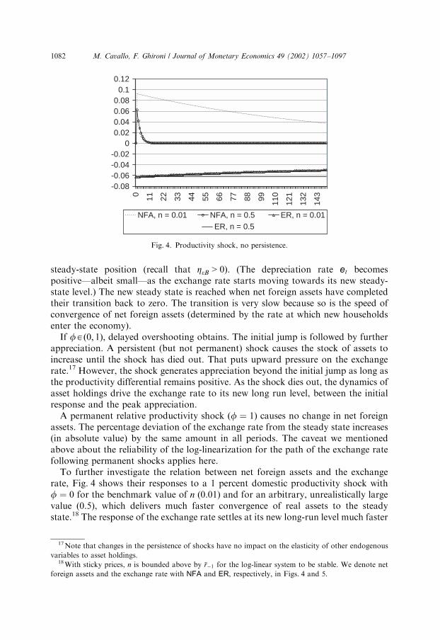
To further investigate the relation between net foreign assets and the exchangerate, Fig. 4 shows their responses to a 1 percent domestic productivity shock withf ¼ 0 for the benchmark value of n (0.01) and for an arbitrary, unrealistically largevalue (0.5), which delivers much faster convergence of real assets to the steadystate.18 The response of the exchange rate settles at its new long-run level much faster

-0.08-0.06-0.04-0.02

00.020.040.060.080.1

0.12

0 11 22 33 44 55 66 77 88 99 110

121

132

143

NFA, n = 0.01 NFA, n = 0.5 ER, n = 0.01ER, n = 0.5

Fig. 4. Productivity shock, no persistence.

17Note that changes in the persistence of shocks have no impact on the elasticity of other endogenous

variables to asset holdings.18With sticky prices, n is bounded above by %r�1 for the log-linear system to be stable. We denote net

foreign assets and the exchange rate with NFA and ER, respectively, in Figs. 4 and 5.


when n ¼ 0:5: Put differently, the response of the exchange rate is closer to that of apure random walk the faster the speed of convergence of net foreign assets to thesteady state. Even if the elasticity of the exchange rate to net foreign assets is verysmall for the parameter values we use ðZeB ¼ 0:0014 [0.0005] when n ¼ 0:01 [0.5]),near non-stationary net foreign assets generate exchange rate dynamics that can bequite different from those of a random walk.

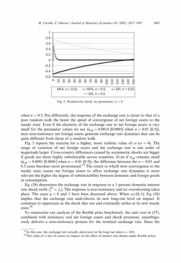
Fig. 5 repeats the exercise for a higher, more realistic value of o ðo ¼ 4Þ: Therange of variation of net foreign assets and the exchange rate is one order ofmagnitude larger. Cross-country differences caused by asymmetric shocks are biggerif goods are more highly substitutable across countries. Even if ZeB remains smallðZeB ¼ 0:0081 [0.0041] when n ¼ 0:01 [0.5]), the difference between the n ¼ 0:01 and0:5 cases becomes more pronounced.19 The extent to which slow convergence to thesteady state causes net foreign assets to affect exchange rate dynamics is morerelevant the higher the degree of substitutability between domestic and foreign goodsin consumption.

Eq. (58) determines the exchange rate in response to a 1 percent domestic interestrate shock (with xDt ¼ xtÞ: The response is non-stationary and no overshooting takesplace. The cases m ¼ 0 and 1 have been discussed above. When mAð0; 1Þ; Eq. (58)implies that the exchange rate undershoots its new long-run level on impact. Itcontinues to appreciate as the shock dies out and eventually settles at its new steadystate.20

To summarize our analysis of the flexible price benchmark, the unit root in (57),combined with stationary real net foreign assets and shock processes, unambigu-ously delivers a non-stationary process for the nominal exchange rate. Since the

-0.6

-0.4

-0.2

0

0.2

0.4

0.6

0.8

1

0 10 20 30 40 50 60 70 80 90 100

110

120

130

140

150

NFA, n = 0.01 NFA, n = 0.5 ER, n = 0.01ER, n = 0.5

Fig. 5. Productivity shock, no persistence, o ¼ 4:

19 In this case, the exchange rate actually depreciates in the long run when n ¼ 0:01:20The value of o has of course no impact on the effect of interest rate shocks under flexible prices.


deviation of net foreign assets from the steady state becomes negligible in finite timefollowing a non-permanent shock, the exchange rate eventually settles on a newlong-run position if shocks are not permanent.21 Notwithstanding the presence of aunit root in the exchange rate, impulse response analysis supports the idea that netforeign asset dynamics help predict the path of the nominal exchange rate to theextent that the elasticity of the latter to net foreign assets is different from zero. Thequantitative relevance of net foreign assets for exchange rate behavior is enhanced iftheir law of motion is near non-stationary and if the elasticity of substitutionbetween domestic and foreign goods is significantly above 1. Finally, the exercise ofthis section shows that price stickiness is not necessary to obtain exchange rate over-or undershooting following exogenous impulses. Endogenous interest rate settingand asset dynamics are sufficient.

5. Sticky prices

The exchange rate continues to be determined by Eq. (54). However, the dynamicsof the real GDP differential (and of all other real variables) following productivityand interest rate shocks are now affected by the markup fluctuations generated bynominal rigidity.

It is possible to prove that o ¼ 1 implies Btþ1 ¼ 0 8t also under sticky pricesregardless of other parameter values. Intuitively, Eq. (40) shows that the GDPdifferential is always zero regardless of productivity and interest rates if the elasticityof substitution between domestic and foreign goods is one. Because countries arestarting off with zero net assets, identical GDP levels imply that the two economieshave identical real resources to allocate to consumption in all periods. Thus, theutility maximizing choice entails cDt ¼ 0 8t:

The system on which we focus our attention for the general case oa1 consists ofEqs. (35), (36), (40), (41), (43)–(46), and (54), combined with our assumptions on theshock processes, xDt ¼ mxDt�1 and ZD

t ¼ fZDt�1: It is hard to obtain an easily

interpretable analytical solution for this system. Thus, we resort to Uhlig’s (1999)numerical implementation of Campbell (1994). The endogenous state vector is½Btþ1; Et;c

Dt ;w

Dt ; y

Dt ; h

Dt ; v

Dt �

0; the vector of other endogenous variables is ½pPPID

t ; cDt �0;

and the vector of exogenous driving forces is ½ZDt ; x

Dt �

0: We include hDt and vDt in thestate vector to avoid singularity problems in the solution. The method returns aunique stable solution for the parameter values we consider. We use the baselineparameterization above, which we repeat for convenience: b ¼ 0:99; r ¼ 0:33; o ¼1:2; a ¼ 0:5; n ¼ 0:01; a1 ¼ 0:5; and a2 ¼ 1:5: We set k to 77, the estimate in Ireland(2001), and y to 6, consistent with Rotemberg and Woodford (1992). These valuesimply that PPI inflation of 1 percent would generate a resource cost of 0.385 percent

21 If n ¼ 0; a favorable shock to home productivity with f ¼ 0 causes domestic net foreign assets to

settle at a new (higher) steady-state level by the beginning of period 1. The exchange rate appreciates at

t ¼ 0; but it depreciates in all following periods, eventually shooting to infinity.


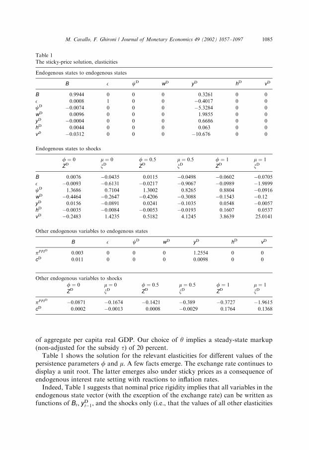
of aggregate per capita real GDP. Our choice of y implies a steady-state markup(non-adjusted for the subsidy t) of 20 percent.

Table 1 shows the solution for the relevant elasticities for different values of thepersistence parameters f and m: A few facts emerge. The exchange rate continues todisplay a unit root. The latter emerges also under sticky prices as a consequence ofendogenous interest rate setting with reactions to inflation rates.

Indeed, Table 1 suggests that nominal price rigidity implies that all variables in theendogenous state vector (with the exception of the exchange rate) can be written asfunctions of Bt; yDt�1; and the shocks only (i.e., that the values of all other elasticities

Table 1

The sticky-price solution, elasticities

Endogenous states to endogenous states

B E cD wD yD hD vD

B 0.9944 0 0 0 0.3261 0 0

E 0.0008 1 0 0 �0.4017 0 0

cD �0.0074 0 0 0 �5.3284 0 0

wD 0.0096 0 0 0 1.9855 0 0

yD �0.0004 0 0 0 0.6686 0 0

hD 0.0044 0 0 0 0.063 0 0

vD �0.0312 0 0 0 �10.676 0 0

Endogenous states to shocks

f ¼ 0 m ¼ 0 f ¼ 0:5 m ¼ 0:5 f ¼ 1 m ¼ 1

ZD xD ZD xD ZD xD

B 0.0076 �0.0435 0.0115 �0.0498 �0.0602 �0.0705

E �0.0093 �0.6131 �0.0217 �0.9067 �0.0989 �1.9899

cD 1.3686 0.7104 1.3002 0.8265 0.8804 �0.0916

wD �0.4464 �0.2647 �0.4206 �0.3088 �0.1543 �0.12

yD 0.0156 �0.0891 0.0241 �0.1035 0.0548 �0.0057

hD �0.0035 �0.0084 �0.0053 �0.0193 0.1607 0.0537

vD �0.2483 1.4235 0.5182 4.1245 3.8639 25.0141

Other endogenous variables to endogenous states

B E cD wD yD hD vD

pPPID

0.003 0 0 0 1.2554 0 0

cD 0.011 0 0 0 0.0098 0 0

Other endogenous variables to shocks

f ¼ 0 m ¼ 0 f ¼ 0:5 m ¼ 0:5 f ¼ 1 m ¼ 1

ZD xD ZD xD ZD xD

pPPID

�0.0871 �0.1674 �0.1421 �0.389 �0.3727 �1.9615

cD 0.0002 �0.0013 0.0008 �0.0029 0.1764 0.1368


are zero, at least for the benchmark parameterization and a number of plausiblealternatives).

The solution for the exchange rate in Table 1 is of the form

Et ¼ Et�1 þ ZeBBt þ ZeyDyDt�1 þ ZeZDZ

Dt þ ZexDx

Dt : ð59Þ

On empirical grounds, the sticky-price solution points to the past GDP differentialas a determinant of the current exchange rate, along with net foreign assetsaccumulated in the previous period. As for the flexible-price case, ZeB is positive andsmall: a capital inflow generates exchange rate appreciation. Accumulation of netforeign debt is associated to higher domestic GDP than foreign because domesticagents supply more labor. The interest rate differential rises in response to a positiveGDP differential, which leads to appreciation. The elasticity to the past GDPdifferential ðZeyD Þ is negative for similar reasons. Sticky prices introduce persistencein the GDP process beyond its dependence on assets accumulated in the previousperiod. (Recall that GDP is measured in units of the consumption basket, i.e., bymultiplying production of domestic goods by their relative price. Stickiness in thelatter introduces stickiness in GDP.) As a consequence of GDP persistence, apositive GDP differential yesterday translates into a higher interest rate differentialtoday and, hence, into appreciation. The negative elasticity to productivity ðZeZD Þreflects the fact that higher domestic productivity generates higher domestic outputdirectly, as in the flexible-price world. Again, this leads to a higher domestic interestrate and appreciation.22 Consistent with uncovered interest parity, an exogenousincrease in ZexD causes the domestic currency to appreciate on impact.

As in the flexible-price world, changes in shock persistence affect only theelasticities to the shocks themselves. The elasticity of assets to productivity ðZBZD Þ isan increasing function of the persistence of productivity shocks for fo1: Intuitively,the more persistent a (non-permanent) favorable productivity shock, the stronger theincentive of households to accumulate assets to smooth consumption ðZyDZD isunambiguously increasing in f). Interestingly, ZBZD is negative in the special casef ¼ 1: The domestic country accumulates debt if there is a permanent favorableshock to relative productivity. The reason is that a permanent favorable productivityshock causes the new long-run level of domestic GDP to be above the initial jumpfollowing the shock (GDP stickiness through relative price persistence is responsiblefor this; see also below). As a consequence, optimal consumption smoothing dictatesthat domestic agents borrow in the anticipation of permanently higher income in thefuture. The relation between ZBxD and the persistence of interest rate shocks ðmÞ isnon-monotonic and less easily interpretable. The elasticity of the exchange rate tothe productivity differential is larger (in absolute value) the more persistent thelatter. As under flexible prices, a more persistent productivity differential generatesanticipation of a more persistent interest rate differential, and hence a largermovement of the exchange rate on impact. As expected, the elasticity of the exchangerate to the relative interest rate shock increases with the persistence of the latter.

22Not surprisingly, if a1 ¼ 0 (interest rates do not react to GDP movements), it is ZeB ¼ ZeyD ¼ ZeZD ¼ 0

also under sticky prices.


5.1. Impulse response analysis

5.1.1. Productivity shock

Fig. 6 shows impulse responses to a 1 percent favorable shock to relative domesticproductivity for the values of f in Table 1.23 Consider the f ¼ 0—case. Underflexible prices, the exchange rate overshoots its new long-run equilibrium on impact.It then converges monotonically to the new steady state. The home countryaccumulates assets in the initial period, which it decumulates back to the steady statealong the transition dynamics. Sticky prices cause a hump-shaped response of netforeign assets and delayed overshooting, as we observed under flexible prices whenthe productivity shock was persistent. The reason for this difference is exactly thatprice-stickiness imparts persistence in the dynamics of the GDP differential asdescribed above. Domestic firms initially lower prices more than foreign firms,though the domestic markup rises relative to foreign to preserve profitability. Labordemand falls (not shown), and so does the real wage. However, these movements arequickly reversed. A more persistent favorable GDP differential causes home agentsto continue accumulating assets in the first periods after the shock. As under flexibleprices, continuing asset accumulation puts upward pressure on the exchange rate.But the added persistence in the GDP differential acts as persistence in productivityunder flexible prices, causing further appreciation. When the GDP differential isclose to zero, the upward pressure on the exchange rate from asset holdings abovethe steady state kicks in, and assets and the exchange rate converge slowly to theirsteady-state levels. Interestingly, the stock market value of the domestic economyrelative to foreign is below the steady state throughout the transition, reflecting thefact that the markup is below the steady state for most of the time. As expected,domestic consumption is (slightly) above foreign.

When the productivity shock is more persistent—fAð0; 1Þ—the dynamics of netforeign assets and the exchange rate are similar, with a hump-shaped response ofassets and delayed exchange rate overshooting. Persistence in productivityintroduces a hump in the response of GDP, consistent with the persistence effectof price rigidity and markup dynamics. (GDP rises with labor demand as the markupfalls after the initial increase.) The markup is above the steady state for longer, whichcauses an initial stock market expansion relative to foreign.

If f ¼ 1; the domestic country borrows from abroad for the reasons describedabove. Domestic GDP climbs to a permanently higher level than foreign over timedue to price stickiness and markup dynamics. (Consumption smoothing causes thedomestic economy to run a debt after a permanent favorable shock to relativeproductivity also in Obstfeld and Rogoff, 1995. The shock has no short-run effect onGDP in their setup.) The exchange rate appreciates in all periods in Fig. 6(appreciation reaches 20 percent 30 years after the shock, though the caveatmentioned above applies here). The relative markup is permanently above the initial

23 In Figs. 6 and 7, net foreign assets in each period ðB1Þ are net foreign assets at the end of that period.

The exchange rate and the PPI inflation and markup differentials are denoted by eps; ppiiD; and mkupD;respectively. The relative interest rate shock is csiD:


steady state (albeit by very little) and relative PPI inflation is permanently lower. Thereal wage differential falls initially, as higher productivity and the initial relativemarkup movement depress domestic labor demand relative to foreign. However,higher long-run GDP at home than abroad results in a positive long-run real wage

φ = 0

0 5 10 15 20 25 30 35 40- 0.03

- 0.02

- 0.01

0

0.01

0.02

0.03

Years after shock

Per

cent

dev

iatio

n fr

om s

tead

y s

tate

B1

eps

0 0.5 1 1.5 2 2.5 3-0.2

0

0.2

0.4

0.6

0.8

1

1.2

1.4Impulse responses to a shock in ZD

Impulse responses to a shock in ZD

Years after shock Years after shock0 0.5 1 1.5 2 2.5 3

Per

cent

dev

iatio

n fr

om s

tead

y st

ate

mkupD

ppiiD

-0.45

-0.35

-0.3

-0.4

-0.2

-0.1

0

-0.25

-0.15

-0.05

0.05Impulse responses to a shock in ZD

Impulse responses to a shock in ZD Impulse responses to a shock in ZD

wD

yD

0 0.5 1 1.5 2 2.5 3-0.4

-0.2

0

0.2

0.4

0.6

0.8

1

1.2

1.4

Years after shock

Per

cent

dev

iatio

n fr

om s

tead

y st

ate

mkupD vD

0 1 2 3 4 5 6 7 8 9 100

0.5

1

1.5

2

2.5x 10-4

Years after shock

Per

cent

dev

iatio

n fr

om s

tead

y st

ate

Per

cent

dev

iatio

n fr

om s

tead

y st

ate

cD

Fig. 6. Productivity shock, sticky prices.


differential. A permanently higher markup causes the domestic stock market valueto rise permanently above foreign. So does domestic consumption.

If one believes that the advent of the ‘new economy’ has shifted U.S. productivitypermanently above foreign, our model provides a qualitative account of empiricalobservations of the past few years. The model also delivers much richer exchangerate dynamics following a productivity shock under sticky prices than its antecedent

φ= 0.5

0 5 10 15 20 25 30 35 40

- 0.02- 0.04

- 0.06- 0.08

- 0.1

- 0.12

0

0.08

0.06

0.040.02

Years after shock

Years after shock

Years after shock Years after shock

Per

cent

dev

iatio

n fr

om s

tead

y st

ate

B1

eps

0 0.5 1 1.5 2 2.5 3 3.5 4Years after shock

0 0.5 1 1.5 2 2.5 3 3.5 4

mkupD

ppiiD

- 0.45

- 0.35

- 0.25

- 0.15

- 0.05

-0.4

-0.3

-0.2

-0.1

0

0.05P

erce

nt d

evia

tion

from

ste

ady

stat

e

wD

yD

0 0.5 1 1.5 2 2.5 3 3.5 4-0.4-0.2

0

0

1.4

1.2

1.0

0.8

0.6

0.4

0.2

Per

cent

dev

iatio

n fr

om s

tead

y st

ate

mkupD

vD

0 1 2 3 4 5 6 7 8 9 100

1

2

3

4

5

6

7

8x 10

_4

Per

cent

dev

iatio

n fr

om s

tead

y st

ate

cD





-0.2

1.4

1.2

1.0

0.8

0.6

0.4

0.2

Per

cent

dev

iatio

n fr

om s

tead

y st

ate

Fig. 6 (continued).


by Obstfeld and Rogoff (1995). The case of a temporary productivity shock is trivialin that model. Supply equations are not binding in the short run, and the shock hasno output effect. A permanent shock causes the exchange rate to appreciatepermanently in the period of the shock. No further dynamics happen and noovershooting is obtained in either case.

0 5 10 15 20 25 30 35 40-30

-25

-20

-15

-10

-5

0Impulse responses to a shock in ZD




Years after shock

Years after shock

Per

cent

dev

iatio

n fr

om s

tead

y st

ate

Per

cent

dev

iatio

n fr

om s

tead

y st

ate

Per

cent

dev

iatio

n fr

om s

tead

y st

ate

Per

cent

dev

iatio

n fr

om s

tead

y st

ate

Per

cent

dev

iatio

n fr

om s

tead

y st

ate

B1eps

mkupD

ppiiD

wD

yD

mkupD

vD

0 0.5 1 1.5 2 2.5 3 3.5 4.54 5Years after shock

0

0

0.5 1 1.5 2 2.5 3 3.5 4.54 5

Years after shock Years after shock0 0.5

3.5

2.5

1.5

0.5

1

4

3

2

1

01.5 2 2.5 3 3.5 4.54 5

01 2 3 4 5 6 7 8 9 10

1

0.8

0.6

0.4

0.2

0.2

0.4

0

_

_

0.18

0.16

0.14

0.12

0.15

0.15

0.05

0.05

0.2

0.2

0.1

0.1

0.08

0.06

0.04

0.02

cD

0

_

_

_

_

φ= 1

Fig. 6 (continued).


5.1.2. Interest rate shock

Fig. 7 shows impulse responses to a 1 percent exogenous increase in domesticinterest rates for the values of m in Table 1. Under flexible prices, the exchange ratejumped immediately to its new long-run equilibrium after an interest rate shock withno persistence ðm ¼ 0Þ: When prices are sticky, the shock affects real variables, whichin turn have an impact on exchange rate dynamics. Higher domestic interest rates

µ = 0

0 5 10 15 20 25 30 35 40-0.7

-0.6

-0.5

0.8

0.7

0.6

0.5

0.4

0.3

0.2

0.1

1.5

0.5

-0.4

-1.5

-1

-0.5

-0.3

-0.35

-0.25

-0.15

-0.05

-0.2

-0.1

-0.3

-0.2

-0.1

0Impulse responses to a shock in csiD

Impulse responses to a shock in csiD Impulse responses to a shock in csiD


Years after shock

Per

cent

dev

iatio

n fr

om s

tead

y st

ate

Per

cent

dev

iatio

n fr

om s

tead

y st

ate

Per

cent

dev

iatio

n fr

om s

tead

y st

ate

Per

cent

dev

iatio

n fr

om s

tead

y st

ate

Per

cent

dev

iatio

n fr

om s

tead

y st

ate

B1

eps

mkupD

ppiiD

wD

yD

mkupD

vD

0

0

0

1 2 3 4 5 6 7 8 9 10

x 10_3

cD

0

-0.1

-0.2

0

1

Years after shock0 0.5 1 1.5 2 2.5 3

Years after shock0 0.5 1 1.5 2 2.5 3

Years after shock Years after shock0 0.5 1 1.5 2 2.5 3

Fig. 7. Interest rate shock, sticky prices.


result in lower PPI inflation at home than abroad, though firms raise the markupcomponent of prices to preserve profitability, and this translates into a higherrelative value of home equity. Domestic labor demand falls below foreign (notshown), and so do the real wage, GDP, and (slightly) consumption. The homeeconomy borrows from foreign to mitigate the fall in consumption. The exchangerate appreciates on impact. Its dynamics in the periods after the shock reflect those of

µ = 0.5 Impulse responses to a shock in csiD

Impulse responses to a shock in csiD



B1

eps

mkupD

ppiiD

wD

yD

mkupD

vD

0 1 2 3 4 5 6 7 8 9 10

x 10_3

cD

0 5 10 15 20 25 30 35 40Years after shock

Years after shock

-0.2

-0.4

-0.6

-0.8

-1

-1.2

-1.4

-1.6

-1.8

0

Per

cent

dev

iatio

n fr

om s

tead

y st

ate

Per

cent

dev

iatio

n fr

om s

tead

y st

ate

0.8

0.6

0.4

0.2

0

-0.4

-0.2

1

Years after shock0 0.5 1 1.5 2 2.5 3.53 4



-0.3

-0.4

-0.35

-0.25

-0.15

-0.05

-0.2

-0.1

Per

cent

dev

iatio

n fr

om s

tead

y st

ate 0

4.5

3.5

2.5

1.5

0.5

Per

cent

dev

iatio

n fr

om s

tead

y st

ate

4

0

1

2

3-1

-2

-3

-0.5

-1.5

-2.5

-3.5Per

cent

dev

iatio

n fr

om s

tead

y st

ate 0

Fig. 7 (continued).


GDP differential and asset holdings. A GDP differential below the steady statepushes the exchange rate upwards, consistent with the lowering of the domesticinterest rate in response to lower GDP. Net foreign assets below the steady statepush the exchange rate downward. Because the elasticity of the exchange rate to theGDP differential ðZeyD Þ is larger than that to assets ðZeBÞ in absolute value, the formereffect prevails, and the exchange rate moves upwards in the first years after the

µ = 1

0

0

1 2 3 4 5 6 7 8 9 10-80

-0.5

-1.5

-1

-2

-70

-60

-50

-40

-30

-20

-10

0


Impulse responses to a shock in csiDImpulse responses to a shock in csiD


Years after shock

0 1 2 3 4 5 6 7 8 9 10Years after shock

Per

cent

dev

iatio

n fr

om s

tead

y st

ate

Per

cent

dev

iatio

n fr

om s

tead

y st

ate

Per

cent

dev

iatio

n fr

om s

tead

y st

ate

Per

cent

dev

iatio

n fr

om s

tead

y st

ate

Per

cent

dev

iatio

n fr

om s

tead

y st

ate

B1eps

mkupD

ppiiD

wD

yD

mkupD

vD

0.1

0.14

0.12

0.08

0.06

0.04

0.02

0

0.1

0.14

0.08

0.06

0.04

0.02

0

- 0.02

cD

Years after shock0 0.5 1 1.5 2 2.5 3.5 4.53 4 5



0.12

30

25

20

15

10

5

0

-5

0.5

Fig. 7 (continued).


shock. However, the effect of asset dynamics on the exchange rate becomespreponderant once the GDP differential has been (almost entirely) re-absorbed.Approximately five years after the shock, the exchange rate starts moving slowlydownward, mirroring the return of assets to the steady state. Eventually, theexchange rate settles on a new long-run position between the impact appreciation inperiod 0 and the level it had reached due to GDP dynamics. Thus, the exchange ratedisplays ‘‘two-ways’’ overshooting following a zero-persistence relative interest rateshock: it shoots below the new long-run equilibrium on impact, but it climbs above itwhen the GDP differential is the main driving force.

If the interest rate shock is persistent—mAð0; 1Þ—the responses of markup, realwage, GDP, and consumption differential become hump-shaped, as the differentialin relative prices adjusts gradually. Deviations from the steady state become morepersistent. The home economy borrows from abroad to sustain consumption.Consider the case m ¼ 0:5: The exchange rate jumps downward and continues toappreciate further until the GDP differential has reached its peak. After that, theexchange rate reverses direction along with GDP and climbs slightly. As in the caseof a shock with no persistence, once the GDP differential is close to zero, assetdynamics take over, and the exchange rate moves downward to its new steady state.In the case of a persistent shock, the exchange rate undershoots its new long-runequilibrium on impact.24

A permanent shock ðm ¼ 1Þ causes domestic PPI inflation to be permanently belowforeign. The domestic markup now falls on impact relative to foreign, though iteventually settles on a slightly higher value. This translates into a permanently higherdomestic equity value. The initially lower markup generates higher labor demand,which mitigates the negative GDP effect of the shock. The real wage differential isabove the steady state for a long time, though its new steady-state level is negative(not shown). The real GDP differential eventually returns to zero from below.Domestic consumption is above foreign for many years, but it eventually settlesbelow, and the domestic economy is permanently in debt. The percentage deviationof the exchange rate from the steady state increases linearly in absolute value. Thenow usual caveat on the consequences of permanent shock for the path of theexchange rate applies. The interest rate shock has permanent real consequences bygenerating non-zero steady-state inflation, which imposes a permanent real cost onthe economy.

As for the case of a productivity shock, the model delivers richer exchange ratedynamics than the benchmark setup in Obstfeld and Rogoff (1995). It brings a newperspective to bear on Dornbusch’s (1976) results on exchange rate overshooting. Inparticular, our model has the potential for reconciling rational behavior and UIP

24Although it is hard to see this from the figure, the new steady-state level is also below the level that the

exchange rate reaches with the further appreciation due to the hump-shaped response of GDP in the first

years after the shock. When m rises to 0:75; the exchange rate converges monotonically to the new steady

state (see Cavallo and Ghironi, 2001). In this case, the size of the net debt accumulated by the home

economy makes up for the small elasticity of the exchange rate to assets.


with the evidence of delayed overshooting in Clarida and Gal!ı (1994) andEichenbaum and Evans (1995).

6. Conclusions

We presented a theory of exchange rate determination that de-emphasizes the roleof exogenous money supply and emphasizes the relation between the exchange rateand net foreign assets and the endogeneity of interest rate setting. Our model buildson a stationary version of Obstfeld and Rogoff (1995). We relied on the method ofundetermined coefficients as in Campbell (1994) and Uhlig (1999) to obtain thesolution. This technique is fully consistent with the forward-looking nature of themodel. It delivers a process equation for the exchange rate rather than a solutionexpressed in the form of an infinite summation of future variables. This facilitatesinterpretation and quantitative work.

We started from a model with flexible prices and PPP. Interest rates are set to reactto CPI inflation and real GDP movements. The solution for the nominal exchangerate exhibits a unit root, consistent with the empirical findings of Meese and Rogoff(1983). However, today’s exchange rate depends also on the stock of real net foreignassets accumulated in the previous period. For plausible parameter values, a capitalinflow (accumulation of net foreign debt) generates appreciation of the exchangerate. The quantitative relevance of net foreign assets for the latter is stronger theslower their convergence to the steady state following shocks and the higher thedegree of substitutability between domestic and foreign goods in consumption.

We introduced price stickiness by assuming that it is costly to change output pricesover time. We investigated the relation between asset holdings and the exchange ratequantitatively using a plausible calibration of the model. When prices are sticky, theexchange rate still exhibits a unit root. The current level of the exchange rate dependson the past GDP differential, along with net foreign assets.

The model yields a number of results on exchange rate overshooting. Underflexible prices, the exchange rate overshoots its new long-run level following atemporary (relative) productivity shock. If the shock is persistent, endogenousmonetary policy and asset dynamics generate delayed overshooting. Endogenousmonetary policy is responsible for exchange rate undershooting after persistent(relative) interest rate shocks. When prices are sticky, temporary shocks to relativeproductivity result in delayed overshooting. So do persistent shocks. Temporaryrelative interest rate shocks cause immediate overshooting. No overshooting mayhappen when interest rate shocks are persistent. Sticky-price dynamics are richerthan in the Obstfeld and Rogoff (1995) model. Our model has the potential forreconciling rational behavior and UIP with the empirical results in Clarida and Gal!ı(1994) and Eichenbaum and Evans (1995).

The flexible-price model delivers exchange rate appreciation after a favorablerelative productivity shock under Taylor-type monetary policy. This is one side ofthe story that one would like to represent formally when trying to explain therecent behavior of the U.S. economy and the dollar exchange rate. However, the


flexible-price model does not generate appreciation cum accumulation of net foreigndebt. Because consumption smoothing is the only motive for asset accumulation, thehome economy accumulates assets rather than debt. The sticky-price modelgenerates appreciation, a net foreign debt, and a stock market expansion after apermanent favorable shock to relative productivity. But it remains to be seenwhether the advent of the ‘‘new economy’’ has shifted U.S. productivity permanentlyabove foreign. Adding capital accumulation as in Backus et al. (1994) is a promisingway of generating the dynamics in the data for non-permanent productivity shocks.This is a direction we will pursue in future work, along with rigorous testing of themodel’s implications and exploring the consequences of deviations from PPP.25

Another possible extension will be the exploration of the performance of alternativepolicy rules.

References

Backus, D.K., Kehoe, P.J., Kydland, F.E., 1994. Dynamics of the trade balance and the terms of trade: the

J-curve? American Economic Review 84, 84–103.

Benigno, G., Benigno, P., 2001. Monetary policy rules and the exchange rate. CEPR Discussion Paper

2807.

Blanchard, O.J., 1985. Debt, deficits, and finite horizons. Journal of Political Economy 93, 223–247.

Branson, W.H., Henderson, D.W., 1985. The specification and influence of asset markets. In: Jones, R.W.,

Kenen, P.B. (Eds.), Handbook of International Economics, Vol. 2, North-Holland, Amsterdam, pp.

749–805.

Calvo, G.A., 1983. Staggered contracts in a utility maximizing framework. Journal of Monetary

Economics 12, 983–998.

Campbell, J.Y., 1994. Inspecting the mechanism: an analytical approach to the stochastic growth model.

Journal of Monetary Economics 33, 463–506.

Cavallo, M., Ghironi, F., 2001. Net foreign assets and the exchange rate: Redux revived. Working Paper

505, Department of Economics, Boston College.

Clarida, R., Gal!ı, J., 1994. Sources of real exchange rate fluctuations: how important are nominal shocks?

Carnegie-Rochester Conference Series on Public Policy, Vol. 41, pp. 1–56.

Clarida, R., Gertler, M., 1997. How the Bundesbank conducts monetary policy. In: Romer, C.D., Romer,

D.H. (Eds.), Reducing Inflation: Motivation and Strategy. University of Chicago Press, Chicago, pp.

363–406.

Clarida, R., Gal!ı, J., Gertler, M., 1998. Monetary policy rules in practice: some international evidence.

European Economic Review 42, 1033–1067.

Corsetti, G., Pesenti, P., 2001. Welfare and macroeconomic interdependence. Quarterly Journal of

Economics 116, 421–445.

Devereux, M.B., 2002. A tale of two currencies: the Asian crisis and the exchange rate regimes of Hong

Kong and Singapore. Review of International Economics, forthcoming.

Dornbusch, R., 1976. Expectations and exchange rate dynamics. Journal of Political Economy 84, 1161–

1176.

Dornbusch, R., Fischer, S., 1980. Exchange rates and the current account. American Economic Review

70, 960–971.

25There is a fast growing empirical literature on the relation between net foreign assets and the real

exchange rate (Lane and Milesi-Ferretti, 2000, 2002) and on the issues this may pose for the U.S. (Obstfeld

and Rogoff, 2001).


Eichenbaum, M., Evans, C.L., 1995. Some empirical evidence on the effects of shocks to monetary policy

on exchange rates. Quarterly Journal of Economics 110, 975–1009.

Ghironi, F., 2000. Macroeconomic interdependence under incomplete markets. Working Paper 471,

Department of Economics, Boston College.

Ireland, P.N., 2001. Sticky-price models of the business cycle: specification and stability. Journal of

Monetary Economics 47, 3–18.

Kollmann, R., 2001. The exchange rate in a dynamic-optimizing business cycle model with nominal

rigidities: a quantitative investigation. Journal of International Economics 55, 243–262.

Kraay, A., Loayza, N., Serv!en, L., Ventura, J., 2000. Country portfolios. NBER Working Paper, 7795.

Lane, P.R., 2001. The new open economy macroeconomics: a survey. Journal of International Economics

54, 235–266.

Lane, P.R., Milesi-Ferretti, G.M., 2000. The transfer problem revisited: net foreign assets and long-run

real exchange rates. CEPR Discussion Paper 2511.

Lane, P.R., Milesi-Ferretti, G.M., 2002. External wealth, the trade balance, and the real exchange rate.

European Economic Review 46, 1049–1071.

Meese, R.A., Rogoff, K., 1983. Empirical exchange rate models of the seventies: do they fit out of sample?

Journal of International Economics 14, 3–24.

Obstfeld, M., Rogoff, K., 1983. Speculative hyperinflations in maximizing models: can we rule them out?

Journal of Political Economy 91, 675–687.

Obstfeld, M., Rogoff, K., 1995. Exchange rate dynamics redux. Journal of Political Economy 103, 624–

660.

Obstfeld, M., Rogoff, K., 2001. Perspectives on OECD economic integration: implications for U.S.

current account adjustment. In: Global Economic Integration: Opportunities and Challenges,

Proceedings of a Symposium Sponsored by the Federal Reserve Bank of Kansas City, pp. 169–208.

Rotemberg, J.J., 1982. Monopolistic price adjustment and aggregate output. Review of Economic Studies

49, 517–531.

Rotemberg, J.J., Woodford, M., 1992. Oligopolistic pricing and the effects of aggregate demand on

economic activity. Journal of Political Economy 100, 1153–1207.

Schmitt-Groh!e, S., Uribe, M., 2001. Closing small open economy models. Unpublished manuscript,

Rutgers University and University of Pennsylvania.

Shiells, C.R., Stern, R.M., Deardorff, A.V., 1986. Estimates of the elasticities of substitution between

imports and home goods for the United States. Weltwirtschaftliches Archiv 122, 497–519.

Smets, F., Wouters, R., 2002. Openness, imperfect exchange rate pass-through and monetary policy.

Presented at the November 2002 Carnegie-Rochester Conference on Public Policy. Journal of

Monetary Economics 49 (this issue).

Taylor, J.B., 1993. Discretion versus policy rules in practice. Carnegie-Rochester Conference Series on

Public Policy, Vol. 39, pp. 195–214.

Uhlig, H., 1999. A toolkit for analyzing nonlinear dynamic stochastic models easily. In: Marimon, R.,

Scott, A. (Eds.), Computational Methods for the Study of Dynamic Economies. Oxford University

Press, Oxford, pp. 30–61.

Weil, P., 1989. Overlapping families of infinitely-lived agents. Journal of Public Economics 38, 183–198.


net foreign assets and the exchange rate: redux...

Documents