nestor documentationimport/export nestor allows a user to export an entire project, located under...
TRANSCRIPT

Nestor DocumentationRelease 0.3.r2
KEA Development Team
May 28, 2019

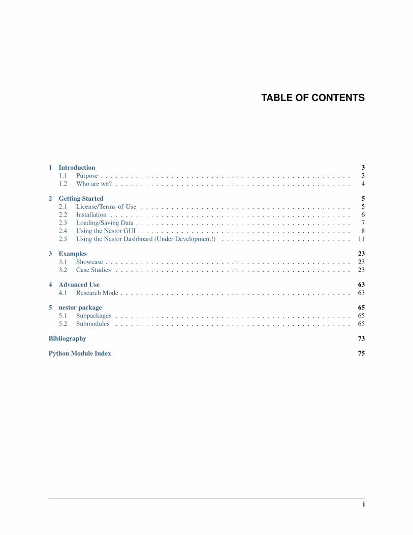
TABLE OF CONTENTS
1 Introduction 31.1 Purpose . . . . . . . . . . . . . . . . . . . . . . . . . . . . . . . . . . . . . . . . . . . . . . . . . . 31.2 Who are we? . . . . . . . . . . . . . . . . . . . . . . . . . . . . . . . . . . . . . . . . . . . . . . . 4
2 Getting Started 52.1 License/Terms-of-Use . . . . . . . . . . . . . . . . . . . . . . . . . . . . . . . . . . . . . . . . . . 52.2 Installation . . . . . . . . . . . . . . . . . . . . . . . . . . . . . . . . . . . . . . . . . . . . . . . . 62.3 Loading/Saving Data . . . . . . . . . . . . . . . . . . . . . . . . . . . . . . . . . . . . . . . . . . . 72.4 Using the Nestor GUI . . . . . . . . . . . . . . . . . . . . . . . . . . . . . . . . . . . . . . . . . . 82.5 Using the Nestor Dashboard (Under Development!) . . . . . . . . . . . . . . . . . . . . . . . . . . 11
3 Examples 233.1 Showcase . . . . . . . . . . . . . . . . . . . . . . . . . . . . . . . . . . . . . . . . . . . . . . . . . 233.2 Case Studies . . . . . . . . . . . . . . . . . . . . . . . . . . . . . . . . . . . . . . . . . . . . . . . 23
4 Advanced Use 634.1 Research Mode . . . . . . . . . . . . . . . . . . . . . . . . . . . . . . . . . . . . . . . . . . . . . . 63
5 nestor package 655.1 Subpackages . . . . . . . . . . . . . . . . . . . . . . . . . . . . . . . . . . . . . . . . . . . . . . . 655.2 Submodules . . . . . . . . . . . . . . . . . . . . . . . . . . . . . . . . . . . . . . . . . . . . . . . 65
Bibliography 73
Python Module Index 75
i

ii

Nestor Documentation, Release 0.3.r2
Nestor is a toolkit for using Natural Language Processing (NLP) with efficient user-interaction to perform structureddata extraction with minimal annotation time-cost.
TABLE OF CONTENTS 1

Nestor Documentation, Release 0.3.r2
2 TABLE OF CONTENTS

CHAPTER
ONE
INTRODUCTION
1.1 Purpose
This application was designed to help manufacturers “tag” their maintenance work-order data according to the methodsbeing researched by the Knowledge Extraction and Applications project at the NIST Engineering Laboratory. The goalof this application is to give understanding to data sets that previously were too unstructured or filled with jargon toanalyze. The current build is in very early alpha, so please be patient in using this application. If you have anyquestions, please do not hesitate to contact us (see Who are we?. )
1.1.1 Why?
There is often a large amount of maintenance data already available for use in Smart Manufacturing systems, butin a currently-unusable form: service tickets and maintenance work orders (MWOs). Nestor is a toolkit for usingNatural Language Processing (NLP) with efficient user-interaction to perform structured data extraction with minimalannotation time-cost.
1.1.2 Features
• Ranks concepts to be annotated by importance, to save you time
• Suggests term unification by similarity, for you to quickly review
• Basic concept relationships builder, to assist assembling problem code and taxonomy definitions
• Strucutred data output as tags, whether in readable (comma-sep) or computation-friendly (sparse-mat) form.
1.1.3 What’s Inside?
Documentation is contained in the /docs subdirectory, and are hosted as webpages and PDF available at readthedocs.io.
Current:
• Tagging Tool: Human-in-the-loop Annotation Interface (pyqt)
• Unstructured data processing toolkit (sklearn-style)
• Vizualization tools for tagged MWOs-style data (under development)
Planned/underway:
• KPI creation and visualization suite
3

Nestor Documentation, Release 0.3.r2
• Machine-assisted functional taxonomy generation
• Quantitative skill assement and training suggestion engine
• Graph Database creation assistance and query tool
1.1.4 Pre-requisites
This package was built as compatible with Anaconda python distribution. See our default requirements file for acomplete list of major dependencies, along with the requirements to run our experimental dashboard or to compile ourdocumentation locally
1.2 Who are we?
This toolkit is a part of the Knowledge Extraction and Application for Smart Manufacturing (KEA) project, within theSystems Integration Division at NIST.
1.2.1 Points of Contact
• Michael Brundage Principal Investigator
• Thurston Sexton Nestor Technical Lead
1.2.2 Contributors:
Name GitHub HandleThurston Sexton @tbsextonSascha Moccozet @saschaMoccozetMichael Brundage @MichaelPBrundageMadhusudanan N. @msngitEmily Hastings @emhastingsLela Bones @lelatbones
1.2.3 Why KEA?
The KEA project seeks to better frame data collection and transformation systems within smart manufacturing ascollaborations between human experts and the machines they partner with, to more efficiently utilize the digital andhuman resources available to manufacturers. Kea (nestor notabilis) on the other hand, are the world’s only alpineparrots, finding their home on the southern Island of NZ. Known for their intelligence and ability to solve puzzlesthrough the use of tools, they will often work together to reach their goals, which is especially important in their harsh,mountainous habitat.
Further reading: [SBHM17][SSB17]
4 Chapter 1. Introduction

CHAPTER
TWO
GETTING STARTED
2.1 License/Terms-of-Use
2.1.1 Software Disclaimer / Release
This software was developed by employees of the National Institute of Standards and Technology (NIST), an agencyof the Federal Government and is provided to you as a public service. Pursuant to title 15 United States Code Section105, works of NIST employees are not subject to copyright protection within the United States.
The software is provided by NIST “AS IS.” NIST MAKES NO WARRANTY OF ANY KIND, EXPRESS, IMPLIEDOR STATUTORY, INCLUDING, WITHOUT LIMITATION, THE IMPLIED WARRANTY OF MERCHANTABIL-ITY, FITNESS FOR A PARTICULAR PURPOSE, NON-INFRINGEMENT AND DATA ACCURACY. NIST doesnot warrant or make any representations regarding the use of the software or the results thereof, including but notlimited to the correctness, accuracy, reliability or usefulness of the software.
To the extent that NIST rights in countries other than the United States, you are hereby granted the non-exclusiveirrevocable and unconditional right to print, publish, prepare derivative works and distribute the NIST software, in anymedium, or authorize others to do so on your behalf, on a royalty-free basis throughout the World.
You may improve, modify, and create derivative works of the software or any portion of the software, and you maycopy and distribute such modifications or works. Modified works should carry a notice stating that you changed thesoftware and should note the date and nature of any such change.
You are solely responsible for determining the appropriateness of using and distributing the software and you assumeall risks associated with its use, including but not limited to the risks and costs of program errors, compliance withapplicable laws, damage to or loss of data, programs or equipment, and the unavailability or interruption of operation.This software is not intended to be used in any situation where a failure could cause risk of injury or damage toproperty.
Please provide appropriate acknowledgments of NIST’s creation of the software in any copies or derivative works ofthis software.
2.1.2 3rd-Party Endorsement Disclaimer
The use of any products described in this toolkit does not imply recommendation or endorsement by the NationalInstitute of Standards and Technology, nor does it imply that products are necessarily the best available for the purpose.
5
Nestor Documentation, Release 0.3.r2
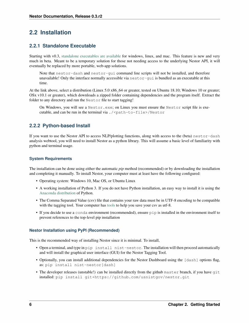
2.2 Installation
2.2.1 Standalone Executable
Starting with v0.3, standalone executables are available for windows, linux, and mac. This feature is new and verymuch in beta. Meant to be a temporary solution for those not needing access to the underlying Nestor API, it willeventually be replaced by more portable, web-app solutions.
Note that nestor-dash and nestor-gui command line scripts will not be installed, and thereforeunavailable! Only the interface normally accessible via nestor-gui is bundled as an executable at thistime.
At the link above, select a distribution (Linux 5.0 x86_64 or greater, tested on Ubuntu 18.10; Windows 10 or greater;OSx v10.1 or greater), which downloads a zipped folder containing dependencies and the program itself. Extract thefolder to any directory and run the Nestor file to start tagging!
On Windows, you will see a Nestor.exe; on Linux you must ensure the Nestor script file is exe-cutable, and can be run in the terminal via ./<path-to-file>/Nestor
2.2.2 Python-based Install
If you want to use the Nestor API to access NLP/plotting functions, along with access to the (beta) nestor-dashanalysis webtool, you will need to install Nestor as a python library. This will assume a basic level of familiarity withpython and terminal usage.
System Requirements
The installation can be done using either the automatic pip method (recommended) or by downloading the installationand completing it manually. To install Nestor, your computer must at least have the following configured:
• Operating system: Windows 10, Mac OS, or Ubuntu Linux
• A working installation of Python 3. If you do not have Python installation, an easy way to install it is using theAnaconda distribution of Python.
• The Comma Separated Value (csv) file that contains your raw data must be in UTF-8 encoding to be compatiblewith the tagging tool. Your computer has tools to help you save your csv as utf-8.
• If you decide to use a conda environment (recommended), ensure pip is installed in the environment itself toprevent references to the top-level pip installation
Nestor Installation using PyPI (Recommended)
This is the recommended way of installing Nestor since it is minimal. To install,
• Open a terminal, and type in pip install nist-nestor. The installation will then proceed automaticallyand will install the graphical user interface (GUI) for the Nestor Tagging Tool.
• Optionally, you can install additional dependencies for the Nestor Dashboard using the [dash] options flag,as: pip install nist-nestor[dash]
• The developer releases (unstable!) can be installed directly from the github master branch, if you have gitinstalled: pip install git+https://github.com/usnistgov/nestor.git
6 Chapter 2. Getting Started
Nestor Documentation, Release 0.3.r2
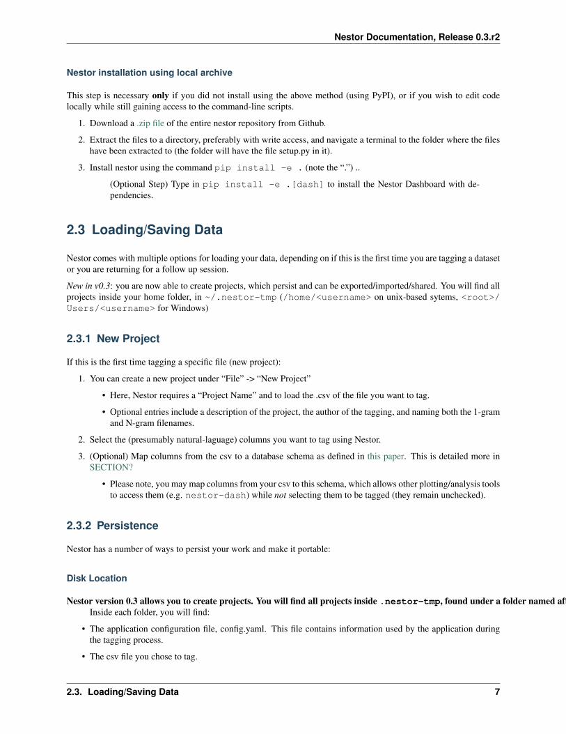
Nestor installation using local archive
This step is necessary only if you did not install using the above method (using PyPI), or if you wish to edit codelocally while still gaining access to the command-line scripts.
1. Download a .zip file of the entire nestor repository from Github.
2. Extract the files to a directory, preferably with write access, and navigate a terminal to the folder where the fileshave been extracted to (the folder will have the file setup.py in it).
3. Install nestor using the command pip install -e . (note the “.”) ..
(Optional Step) Type in pip install -e .[dash] to install the Nestor Dashboard with de-pendencies.
2.3 Loading/Saving Data
Nestor comes with multiple options for loading your data, depending on if this is the first time you are tagging a datasetor you are returning for a follow up session.
New in v0.3: you are now able to create projects, which persist and can be exported/imported/shared. You will find allprojects inside your home folder, in ~/.nestor-tmp (/home/<username> on unix-based sytems, <root>/Users/<username> for Windows)
2.3.1 New Project
If this is the first time tagging a specific file (new project):
1. You can create a new project under “File” -> “New Project”
• Here, Nestor requires a “Project Name” and to load the .csv of the file you want to tag.
• Optional entries include a description of the project, the author of the tagging, and naming both the 1-gramand N-gram filenames.
2. Select the (presumably natural-laguage) columns you want to tag using Nestor.
3. (Optional) Map columns from the csv to a database schema as defined in this paper. This is detailed more inSECTION?
• Please note, you may map columns from your csv to this schema, which allows other plotting/analysis toolsto access them (e.g. nestor-dash) while not selecting them to be tagged (they remain unchecked).
2.3.2 Persistence
Nestor has a number of ways to persist your work and make it portable:
Disk Location
Nestor version 0.3 allows you to create projects. You will find all projects inside .nestor-tmp, found under a folder named after the chosen project name given at creation.Inside each folder, you will find:
• The application configuration file, config.yaml. This file contains information used by the application duringthe tagging process.
• The csv file you chose to tag.
2.3. Loading/Saving Data 7

Nestor Documentation, Release 0.3.r2
• The single token vocabulary file
• The multiple token vocabulary file
By default (if not changed at the time of project creation) the filenames for the vocab files are respectivelyvocab1g.csv and vocabNg.csv.
Import/Export
Nestor allows a user to export an entire project, located under “File” -> “Export Project”, saving it as a portable .zipor .tar file, which can be easily shared among different users of Nestor.
If you are returning to tag a previously tagged dataset, you can either “Open Project,” found in .nestor-tmp, or“Import Project” from a .zip or .tar archive in another location.
You can additionally make use of previous work, such as other projects, by importing from vocabulary sheets that weresaved from previous tagging sessions. This option is available under the “Auto-populate>From CSV” toolbar dropdown menu. The user can select either single word or Multi-Word vocabulary, and select a compatible csv vocabulary,accordingly. Un-annotated words in the current project that are defined in the selected CSV will be updated with theannotations within.
Research mode
If you decide to use the research mode, a new project folder will be added to .nestor-tmp. In this case, additionalfolders will be added inside the project folder. These folders will be named after your chosen criteria. For example, ifyou choose inside the research mode to save your project according to percentage of tokens tagged, then a new foldernamed percentage will appear in your project folder. This percentage folder will contain a version of your vocab filesat a certain percentage.
2.4 Using the Nestor GUI
2.4.1 Settings
This window helps to set various parameters that control how Nestor behaves during the process of tagging. It can beaccessed at any time during the tagging process by going to Python -> Preferences on a Mac. Similar settings can befound for Windows and Linux machines too. (If you are a first time user, or do not really want to change the defaultsettings, it is perfectly fine to leave these settings as they are).
Special Replace
Number of words listed
This setting controls the number of word tokens from your data, that are displayed for tagging. For example, youmight be interested in tagging only the top 1000 words from your data. The ordering is decided based on a measure ofimportance called the *tf-idf* score.
Similarity for ticked words
Recall that Nestor shows you a list of similar words (and check boxes) for each word that you are tagging. You cancontrol which words you want to be ticked by default, when you are tagging. This is done by changing the setting forhow similar are the tagged word and the word in the list, for the similar word to be ticked by default.
8 Chapter 2. Getting Started

Nestor Documentation, Release 0.3.r2
Threshold for List of Similar Words
2.4.2 Single Word Tagging
The Single word analysis tab of Nestor allows the user to classify and tag individual words. Likewise, theMulti word analysis tab will allow classification and tagging of two word phrases.
Word annotation Overview
Present on these tabs are several boxes, which let you interface with concepts found in your data, and assist you inannotating them First is the Word annotation” box, which has four columns:
• words: Also called “tokens”. Single words are presented in order of importance with respect to the user-loadeddata.
• classification: The user’s classification, or “tag-type”, are stored here
• tag: This column will display the given “alias” (cannonical representation) defined for the given word/token
• note: This column stores any relevant notes from picking a given alias or classification.
Similar Words
The “Similar words from csv” box will present similar words to the highlighted selection in the “Words” column.These suggestions are taken directly from the user-loaded data. The slider on the bottom of this box can be adjustedto view more or less words, with decreasing similarity score further down the list. The user can select the words thatshould share a cannonical representation (alias) checking the checkbox.
For example, the user might highlight “replace” and decide that the “repalce” suggestion should refer tothe same tag, by checking the box. Note - all selected words will receive the same alias, classification,and notes.
If the user hovers over the word in this column, a box will appear and display examples that contain the word from theloaded data
User-Input
The “Tag current word” box contains three different fields:
• Preferred Alias: The user can input a preferred alias for the selected word any checked similar words.
• Classification: The user can select the classification for the selected word and checked similar words.The user has five options for classifications in v0.3
– Item
– Problem
– Solution
– Ambiguous (Unknown)
– Irrelevant (Stop-Word)
Ambiguous words will commonly arise in cases where surrounding words are needed to know the “right”classification. These can then be classified in the Multi word analysis tab.
2.4. Using the Nestor GUI 9

Nestor Documentation, Release 0.3.r2
• Notes (if necessary): The user can type notes for a specific word and checked similar words here. The “OverallProgress” at the bottom of the app will track how much progress is completed while the user has annotated wordsin the single word analysis tab. The next word button allows the user to navigate between different words whenannotated.
2.4.3 Multi Word Tagging
The Multi word analysis tab allows the user to classify two word phrases. There are the same four boxes in the WordAnnotation window of nestor as the Single word analysis tab, with a few changes.
Special options
The “Word Composition” box (replaces “Similar words”) provides the user with the information on each constituenttoken comprising the two word phrase.
For example “Replace Hydraulic” will give the user all of the previously stored information for both“Replace” and “Hydraulic” tokens.
The “Tag current words” tab has added/changed the following options from before, as well, to capture meanings forthe bi-gram as a whole:
• Classification: There are two new options to account for:
– Problem Item
– Solution Item
The “Overall Progress” at the bottom of the this tab will track how much progresshas been made specifically onannotated words in the Multi word analysis tab.
Auto-classification
The user can choose auto-populate the classification column on the multi-word tab using the “Auto-populate>Multi word from Single word vocabulary” toolbar drop down menu. This applies a set of logic rules toguess what classification a particular multi-word should receive, based on its constituents.
Note: auto-populated classifications must still be verified by the user. This is done upon entering/keepingthe alias annotation. Only then will it be counted as “complete”
Nestor v0.3 provides the user with predefined rules based on auto population.
• Problem + Item = Problem Item
• Solution + Item = Solution Item
• Item + Item = Item
• Problem + Solution = Irrelevant
Additionally, Nestor will suggest a default alias for word1+word2, namely, word1_word2.
2.4.4 Reporting and Data Transfer
After a sufficient time spent annotating concepts from your corpus, you might like to know what coverage yourannotation has on the detected information within. Nestor provides some metrics and functions on the Report tab,both for exporting your hard work and giving you visual feedback on just how far you’ve come.
First, you will need to process the data using your annotations!
10 Chapter 2. Getting Started

Nestor Documentation, Release 0.3.r2
Always start by pressing the UPDATE TAG EXTRACTION button.
Exporting
Nestor parses through the original text and unifies detected words into the tags you have now created. This is done intwo ways: human-readable (CSV) and binary file store (HDFS)
• create new CSV: a new csv, containing your mapped column headers and new headers for each type of tag,will be exported. Each work-order will now have a list of tags of each type in its corresponding cell. Tags notannotated explicitly will be ommitted.
• create a HDFS (binary): This is a rapid-access filestore (*.h5), excellent for powering visualizations or analysisin other toolkits. Three keys represent three automatically created tables containing your annotated data:
– df: columns from original dataset whose csv headers have been mapped
– tags: binary tag-occurrence matrix for each tag-document pair
– rels PI/SI-document pair occurrence matrix.
The binary file is a requirement to utilize the (beta) nestor-dash functionality. You can use the dashboard byuploading your .h5 file to the dashboard, provided you have marked at least one column as being a .name type (e.g.machine.name is “Asset ID”, technician.name is Technician, etc.)
Progress Report
The bottom half of this window contains various metrics for annotation rates in a table, along with a histogram thatshows a distribution of “completion” over all entries in your corpus. This is the completion-fraction distribution, where“1.0” means all extracted tokens in a work-order have a valid user-given tag and classification, while “0.0” means thatnone of them are annotated.
2.5 Using the Nestor Dashboard (Under Development!)
This tutorial discusses the usage of the Nestor Dashboard. The Dashboard is intended to provide simple, yet insightfulviews into the data contained in Maintenance Work Orders (MWOs). It is a set of visualizations that are pivotedaround various maintenance aspects, such as by machine, technician, problem, and so on. It derives its informationfrom the raw MWOs themselves, as well as the tagged knowledge that is output from the NIST Nestor Tagging Tool.The Nestor Dashboard is visualised on a browser for ease of navigation and to remove dependencies on operatingsystems or other installed software.
2.5.1 Starting the Dashboard Server
1. Open a terminal window
Linux Ctrl + Alt + T
Windows Windows + R -> Type ‘cmd’
Mac + Space -> Type ‘Terminal’
2. Launch the Dashboard Server by typing in nestor-dash
2.5. Using the Nestor Dashboard (Under Development!) 11

Nestor Documentation, Release 0.3.r2
3. This starts up a server for the visualization. Note that the address of the server is output on the terminal window.In this case, it is seen on the last line as‘‘http://127.0.0.1:5000/‘‘. Copy this address.
12 Chapter 2. Getting Started

Nestor Documentation, Release 0.3.r2
4. Open a web browser, and Paste the address from the previous step. The application called Nestor VisualDashboard should start up and you will see the initial welcome screen.
2.5. Using the Nestor Dashboard (Under Development!) 13

Nestor Documentation, Release 0.3.r2
2.5.2 Uploading Data Files
Note: For the current version of the dashboard, visualization is limited to datasets containing “Machine Name” and“Maintenance Technician” entries. Ensure these have been labeled for export in the tagging tool!
1. To immediately start visualizing your data, you need to upload a .csv or .h5 file that was output from the NISTNestor Tagging Tool. To do so, click on the Upload File button. This brings up the page to upload a .csv or .h5file. Click on Choose File and select a file. In this case, the file MWOs_anon.h5 is selected.
After the upload is complete, the Dashboard shows the list of currently uploaded files.
14 Chapter 2. Getting Started

Nestor Documentation, Release 0.3.r2
2.5.3 Viewing Visualizations on Nestor Dashboard
1. Now click on Nestor Dashboard at the top left corner. It brings up the overview page for all visualizations.Currently, there are 3 types incorporated. These are, - Bar Graph - Node-Link Diagram - Flow Diagram
2. Bar Chart: This helps to quickly visualize the relative counts of various factors. For example, in this dataset,the various Solutions (S), Problems (P) and Items (I) can be seen for Machines. It is seen here that for the
2.5. Using the Nestor Dashboard (Under Development!) 15

Nestor Documentation, Release 0.3.r2
machine B2, replaced is the most frequent solution and alarm is the most frequent problem. Similarly, turret isthe major item of concern.
To derive insights about other machines, click on the drop-down on the right side.
Also, you can vary the amount of data being displayed by changing the n_thres slider.
16 Chapter 2. Getting Started

Nestor Documentation, Release 0.3.r2
Instead of viewing all Solutions, Problems and Items in a sorted manner, it is also possible to group them individually.
It is also possible to view the bar chart for various technicians instead of machines by using the dropdown.
2.5. Using the Nestor Dashboard (Under Development!) 17

Nestor Documentation, Release 0.3.r2
The raw data that these visualizations derive from, are also available.
3. Node-Link Diagram: The second type of visualization is the Node-Link diagram. It helps show the connectionsand the strength of the connections between various items, problems and solutions, as a Graph.
18 Chapter 2. Getting Started

Nestor Documentation, Release 0.3.r2
As with the other visualizations, it is easy to switch between Technicians, Machines, and control the thresholds forvisualization. There are values that can be controlled for both the nodes themselves and the strengths of the linksbetween them.
2.5. Using the Nestor Dashboard (Under Development!) 19

Nestor Documentation, Release 0.3.r2
4. Flow Diagram: The Sankey Flow Diagram is another kind of visualization that helps to see the category-wiseconnections. Simultaneously, it is also possible to see the severity of the category itself, such as a solution actionor the item involved. The strength of the relations are proportional to the width of the line connecting the entitiesat either end.
20 Chapter 2. Getting Started

Nestor Documentation, Release 0.3.r2
The weighting methods for the flow diagram can be varied between cosine and count based weights.
2.5. Using the Nestor Dashboard (Under Development!) 21

Nestor Documentation, Release 0.3.r2
22 Chapter 2. Getting Started

CHAPTER
THREE
EXAMPLES
3.1 Showcase
Key features of the nestor toolkit, illustrated.
in progress
3.2 Case Studies
Longer-form, more complete examples of analysis completed for specific datasets.
3.2.1 Manufacturing Maintenance Case Study
Say we have a large amount of historical maintenance work-order (MWO) data stored up, but we don’t quite knowwhat to do with it yet. This case study will walk through the initial parsing of the MWO natural-language data from thetechnicians, to some preliminary analysis of machines, and finally visualization of potential failure modes maintenancerequest types. Hopefully it will give you a good idea of how Nestor can assist you in analyzing the rich, existing datain your MWO’s, and how easy it can be to correlate it to other fields you might be recording.
The primary workflow for Nestor in this case study (when used as a python library) is:
1. Import data, determining
• what columns contain useful (well-defined) categories
• what columns contain natural language to be tagged with the Nestor UI
• what columns could be used for date-stamping/time-series analysis
2. Perform any cleaning necessary on categorical and time-series data.
• This is not necessarily within the scope of Nestor, but:
• Python+Pandas makes it fairly straight forward
• and compatible with the Nestor output tags!
3. Tag natural language data using Nestor/NestorUI
• Nestor can give you initial statistics about your data, immediately, but:
• Nestor is built as a human-in-the-loop tool, meaning that
• you will be a crucial part of the process, and Nestor makes implementing your annotation lightning-fast.
4. Import the tags created by Nestor, and perform analyses
23

Nestor Documentation, Release 0.3.r2
• Nestor UI is designed to create a vocabulary file, quickly mapping discovered concepts to clean tags.
• we’ve also built several tools to help you perform initial analyses on the tags (with more to come!)
We’ll start by loading up some common packages and setting our plotting style (for consistency):
[1]: from pathlib import Pathimport numpy as npimport pandas as pdimport seaborn as snsimport matplotlib.pyplot as plt%matplotlib inline
/home/tbsexton/anaconda3/lib/python3.6/importlib/_bootstrap.py:219: RuntimeWarning:→˓numpy.dtype size changed, may indicate binary incompatibility. Expected 96, got 88return f(*args, **kwds)
/home/tbsexton/anaconda3/lib/python3.6/importlib/_bootstrap.py:219: RuntimeWarning:→˓numpy.dtype size changed, may indicate binary incompatibility. Expected 96, got 88return f(*args, **kwds)
[2]: def set_style():# This sets reasonable defaults for font size for a figure that will go in a papersns.set_context("paper")# Set the font to be serif, rather than sanssns.set(font='serif')# Make the background white, and specify the specific font familysns.set_style("white", {
"font.family": "serif","font.serif": ["Times", "Palatino", "serif"]
})set_style()
For the interactive plots we’ll need Holoviews, with the Bokeh backend:
Data Preparation
Import Data
Nestor will be parsing through the NLP data soon, but first we need to determine what else might be useful for us. Inthis case study, we’ll be using the recorded machine number, the date the MWO was recieved, technician names, andof course, the written descriptions left by our technicians.
In this particular case, we’ll be focusing primarily on the (anonymized) machine types A and B.
[3]: data_dir = Path('../..')/'data'/'sme_data'df = pd.read_csv(data_dir/'MWOs_anon.csv')
df.date_received = pd.to_datetime(df.date_received)print(f'There are {df.shape[0]} MWO\'s in this dataset')
There are 3438 MWO’s in this dataset
[4]: # example data:df.loc[df.mach.str.contains('A\d|B\d', na=False),
['mach', 'date_received', 'issue', 'info', 'tech']].head(10)
[4]: mach date_received issue \0 A5 2015-01-14 No power
(continues on next page)
24 Chapter 3. Examples

Nestor Documentation, Release 0.3.r2
(continued from previous page)
2 A18 2015-02-27 Check / Charge Accumulators3 A23 2015-02-27 Hyd leak at saw atachment4 A24 2015-02-27 CS1008 setup change over / from ARC10045 A27 2015-02-27 Gears on saw attachment tight and grinding per...6 A33 2015-02-27 Check and charge Accumulators7 A8 2015-02-27 St# 14 milling spindle repairs8 B2 2015-02-27 Hydraulic leak9 B3 2015-02-27 Turrets leaking A & B10 B5 2015-02-27 Spindle carrier not indexing / Over Feed
info \0 Replaced pin in pendant and powered machine -P...2 Where OK3 Replaced seal in saw attachment but still leak...4 Completed / Threading unit rewired5 Replaced saw attachment with rebuilt unit / Re...6 Checked and charged7 Reapired8 Replaced ruptured hydraulic line Side B9 Turrets removed and cleaned of chhips10 NaN
tech0 angie_henderson, michele_williams2 nathan_maldonado3 michele_williams4 ethan_adams, michele_williams5 michele_williams6 cristian_santos7 michele_williams8 gina_moore, dylan_miller9 nathan_maldonado10 gina_moore, dylan_miller
Starting Nestor
The first thing we can do is collect, combine, and cleanse our NLP data, to get a better idea of what it looks like goinginto Nestor. To do this, let’s import the main text mining module in Nestor, nestor.keyword, which helps us withkeyword definition and extraction.
The NLPSelect object is a transformer in the style of scikit-learn, which will take in defined names forcolumns containing our original NLP data, and transform that data with it’s .transform() method.
[5]: from nestor import keyword as kex# merge and cleanse NLP-containing columns of the datanlp_select = kex.NLPSelect(columns = ['issue', 'info'])raw_text = nlp_select.transform(df)
/home/tbsexton/anaconda3/lib/python3.6/importlib/_bootstrap.py:219: RuntimeWarning:→˓numpy.dtype size changed, may indicate binary incompatibility. Expected 96, got 88return f(*args, **kwds)
/home/tbsexton/anaconda3/lib/python3.6/importlib/_bootstrap.py:219: RuntimeWarning:→˓numpy.dtype size changed, may indicate binary incompatibility. Expected 96, got 88return f(*args, **kwds)
3.2. Case Studies 25

Nestor Documentation, Release 0.3.r2
Let’s see what the most common MWO’s in our data look like, without the punctuation or filler-words to get in theway:
[6]: raw_text.value_counts()[:10]
[6]: base cleaning requested completed 15broken bar feeder chain repaired 14base needs to be cleaned completed 7broken feeder chain repaired 5chip conveyor jam cleared 5bar feeder chain broken repaired 5bar loader chain broken repaired 5base clean completed 3replace leaking dresser control valve replaced 3workzone light inop 3dtype: int64
Interesting. We see a number of repetitive base-cleaning requests being entered in identically, along with some requeststo fix a broken chain on the bar-feeder. However, there’s alarmingly verbatim repeats, and we see a lot of overlap evenin the top 10 there. This is where Nestor comes in.
Similar to the above, we can make a TokenExtractor object that will perform statistical analysis on our corpus ofMWO’s, and return the concepts it deems “most important”. There’s a lot in here, but essentially we will get an outputof the most important concepts (as tokens) in our data. We do this with the scikit-learn TfIdfVectorizer tool(which transforms our text into a bag-of-words vector model), along with some added features, like a method to scoreand rank individual concepts.
Let’s see what tokens/concepts are most important:
[7]: tex = kex.TokenExtractor()toks = tex.fit_transform(raw_text) # bag of words matrix.
print('Token\t\tScore')for i in range(10):
print(f'{tex.vocab_[i]:<8}\t{tex.scores_[i]:.2e}')
Token Scorereplaced 1.86e-02broken 9.68e-03st 9.51e-03unit 8.41e-03inop 7.27e-03motor 7.21e-03spindle 7.17e-03leak 6.88e-03repaired 6.75e-03valve 6.74e-03
These are small scores, but they’re normalized to add to 1:
[8]: tex.scores_.sum()
[8]: 1.0
Note that the current default is to limit the number of extracted concepts to the top 5000 (can be modified in theTokenExtractor kwargs, but in practice should be more than sufficient.
26 Chapter 3. Examples
Nestor Documentation, Release 0.3.r2
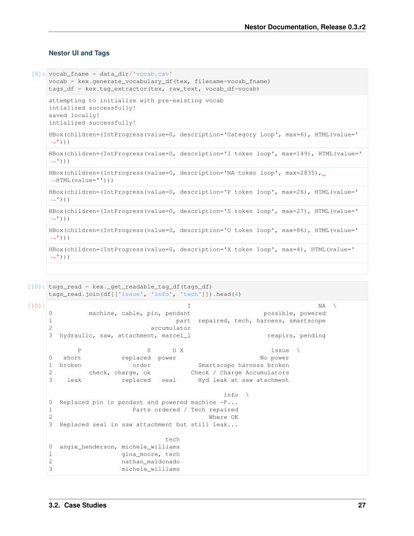
Nestor UI and Tags
[9]: vocab_fname = data_dir/'vocab.csv'vocab = kex.generate_vocabulary_df(tex, filename=vocab_fname)tags_df = kex.tag_extractor(tex, raw_text, vocab_df=vocab)
attempting to initialize with pre-existing vocabintialized successfully!saved locally!intialized successfully!
HBox(children=(IntProgress(value=0, description='Category Loop', max=6), HTML(value='→˓')))
HBox(children=(IntProgress(value=0, description='I token loop', max=149), HTML(value='→˓')))
HBox(children=(IntProgress(value=0, description='NA token loop', max=2835),→˓HTML(value='')))
HBox(children=(IntProgress(value=0, description='P token loop', max=26), HTML(value='→˓')))
HBox(children=(IntProgress(value=0, description='S token loop', max=27), HTML(value='→˓')))
HBox(children=(IntProgress(value=0, description='U token loop', max=86), HTML(value='→˓')))
HBox(children=(IntProgress(value=0, description='X token loop', max=4), HTML(value='→˓')))
[10]: tags_read = kex._get_readable_tag_df(tags_df)tags_read.join(df[['issue', 'info', 'tech']]).head(4)
[10]: I NA \0 machine, cable, pin, pendant possible, powered1 part repaired, tech, harness, smartscope2 accumulator3 hydraulic, saw, attachment, marcel_l reapirs, pending
P S U X issue \0 short replaced power No power1 broken order Smartscope harness broken2 check, charge, ok Check / Charge Accumulators3 leak replaced seal Hyd leak at saw atachment
info \0 Replaced pin in pendant and powered machine -P...1 Parts ordered / Tech repaired2 Where OK3 Replaced seal in saw attachment but still leak...
tech0 angie_henderson, michele_williams1 gina_moore, tech2 nathan_maldonado3 michele_williams
3.2. Case Studies 27

Nestor Documentation, Release 0.3.r2
[11]: # how many instances of each keyword class are there?print('named entities: ')print('I\tItem\nP\tProblem\nS\tSolution\nR\tRedundant')print('U\tUnknown\nX\tStop Word')print('tagged tokens: ', vocab[vocab.NE!=''].NE.notna().sum())print('total tags: ', vocab.groupby("NE").nunique().alias.sum())vocab.groupby("NE").nunique()
named entities:I ItemP ProblemS SolutionR RedundantU UnknownX Stop Wordtagged tokens: 518total tags: 294
[11]: NE alias notes scoreNE
1 2 1 2485I 1 149 8 280P 1 26 1 63S 1 27 1 57U 1 86 6 113X 1 4 1 4
[12]: # tag-completeness of work-orders?tag_pct, tag_comp, tag_empt = kex.get_tag_completeness(tags_df)
nbins = int(np.percentile(tags_df.sum(axis=1), 90))print(f'Docs have at most {nbins} tokens (90th percentile)')
sns.distplot(tag_pct.dropna(), bins=nbins, kde_kws={'cut':0})plt.xlim(0.1, 1.0)plt.xlabel('precision (PPV)')
Tag completeness: 0.72 +/- 0.19Complete Docs: 514, or 14.95%Empty Docs: 20, or 0.58%Docs have at most 13 tokens (90th percentile)
/home/tbsexton/anaconda3/lib/python3.6/site-packages/scipy/stats/stats.py:1713:→˓FutureWarning: Using a non-tuple sequence for multidimensional indexing is→˓deprecated; use `arr[tuple(seq)]` instead of `arr[seq]`. In the future this will be→˓interpreted as an array index, `arr[np.array(seq)]`, which will result either in an→˓error or a different result.return np.add.reduce(sorted[indexer] * weights, axis=axis) / sumval
[12]: Text(0.5,0,'precision (PPV)')
28 Chapter 3. Examples

Nestor Documentation, Release 0.3.r2
Context Expansion (simplified)
Nestor now has a convenience function for generating 1- and 2-gram tokens, and extracting “good” tags from yourMWO’s once given the 1- and 2-gram vocabulary files generated by the nestor-gui application. This makes ourlife easier, though the functionality is planned to be deprecated and replaced by a more robust pipelining tool fashinedafter the Scikit-Learn Pipeline model.
[13]: vocab = pd.read_csv(vocab_fname, index_col=0)vocab2 = pd.read_csv(data_dir/'2g_vocab.csv', index_col=0)
tag_df, tag_relation, NA_df = kex.ngram_keyword_pipe(raw_text, vocab, vocab2)
calculating the extracted tags and statistics...
ONE GRAMS...intialized successfully!
HBox(children=(IntProgress(value=0, description='Category Loop', max=6), HTML(value='→˓')))
HBox(children=(IntProgress(value=0, description='I token loop', max=149), HTML(value='→˓')))
HBox(children=(IntProgress(value=0, description='NA token loop', max=2835),→˓HTML(value='')))
HBox(children=(IntProgress(value=0, description='P token loop', max=26), HTML(value='→˓')))
HBox(children=(IntProgress(value=0, description='S token loop', max=27), HTML(value='→˓')))
HBox(children=(IntProgress(value=0, description='U token loop', max=86), HTML(value='→˓')))
HBox(children=(IntProgress(value=0, description='X token loop', max=4), HTML(value='→˓')))
found bug! None
(continues on next page)
3.2. Case Studies 29

Nestor Documentation, Release 0.3.r2
(continued from previous page)
TWO GRAMS...intialized successfully!
HBox(children=(IntProgress(value=0, description='Category Loop', max=8), HTML(value='→˓')))
HBox(children=(IntProgress(value=0, description='I token loop', max=625), HTML(value='→˓')))
HBox(children=(IntProgress(value=0, description='NA token loop', max=1833),→˓HTML(value='')))
HBox(children=(IntProgress(value=0, description='P token loop', max=28), HTML(value='→˓')))
HBox(children=(IntProgress(value=0, description='P I token loop', max=408),→˓HTML(value='')))
HBox(children=(IntProgress(value=0, description='S token loop', max=26), HTML(value='→˓')))
HBox(children=(IntProgress(value=0, description='S I token loop', max=427),→˓HTML(value='')))
HBox(children=(IntProgress(value=0, description='U token loop', max=1466), HTML(value=→˓'')))
HBox(children=(IntProgress(value=0, description='X token loop', max=187), HTML(value='→˓')))
We can also get a version of the tags that is human-readable, much like the tool in nestor-gui. Though less usefulfor plotting/data-analysis, this is great for a sanity check, or for users that prefer visual tools like Excel.
[14]: all_tags = pd.concat([tag_df, tag_relation])tags_read = kex._get_readable_tag_df(all_tags)tags_read.head(10)
[14]: I P P I \0 cable, machine, pendant, pin short1 part broken2 accumulator3 attachment, hydraulic, marcel_l, saw, saw atta... leak4 thread, thread unit, unit5 alex_b, attachment, gear, saw, saw attachment,...6 accumulator7 mill, spindle, station8 hydraulic, hydraulic line, line leak, rupture9 turret leak
S S I U0 replaced power1 order2 charge, check, ok3 replaced seal4 setup change5 rebuild, remove, replaced6 charge, check7 repair 14
(continues on next page)
30 Chapter 3. Examples

Nestor Documentation, Release 0.3.r2
(continued from previous page)
8 replaced9 clean, remove
Measuring Machine Performance
The first thing we might want to do is determine which assets are problematic. Nestor outputs tags, which need to bematched to other “things of interest,” whether that’s technicians, assets, time-stamps, etc. Obviously not every datasetwill have every type of data, so not all of these analyses will be possible in every case (a good overview of what keyperformance indicators are possible with what data-type can be found here).
Since we have dates and assets associated with each MWO, let’s try to estimate the failure inter-arrival times formachines by type and ID.
Failure Inter-arrival Times, by Machine
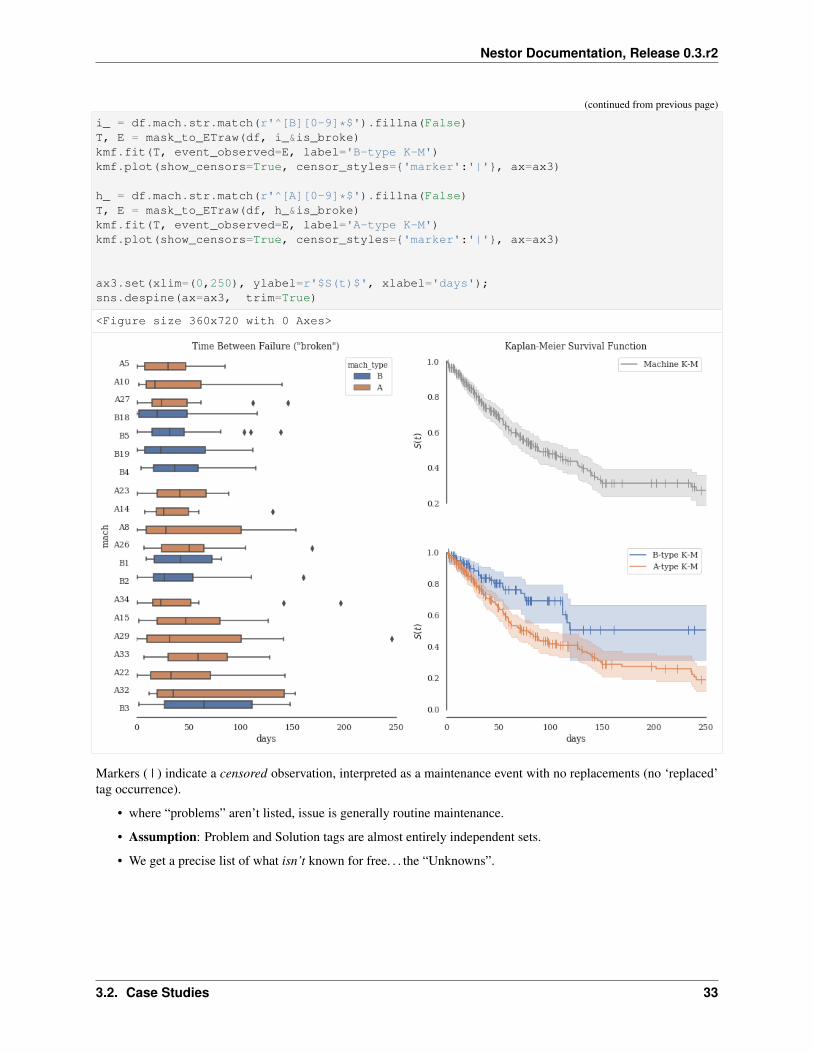
Ordered by total occurences (i.e. “distribution certainty”)
• Time between occurences of broken tag.
• low → bad
• e.g. A34, B19, and A14 all seem rather low
What could be the central problems with these machines? While we’re at it, let’s use the wonderful library Lifelines tocalculate the Survival functions of our different machine types. We can again use tags to approximate relevant data weotherwise would not have had: censoring of observations is not obvious, but we can guess that replacements (withoutbroken) generally indicate a machine was swapped before full breakdown/end-of-life.
[18]: import warningswarnings.simplefilter(action='ignore')
# make sure Pandas knows our column is a proper Datetime.idx_col = pd.DatetimeIndex(df.date_received)
# match the A and B machines, checking if they were "broken"h_or_i = (df
.mach
.str
.match(r'^[AB][0-9]*$')
.fillna(False))is_broke = (tag_df.P['broken']>0)cond = h_or_i & is_brokesample_tag = tag_df.loc[cond,tag_df.loc[cond].sum()>1]sample_tag.columns = (sample_tag
.columns
.droplevel(0))
# Add tags back to original datasample_tag = pd.concat([sample_tag, df.mach[cond]], axis=1)sample_tag['date'] = idx_col[cond]sample_tag.loc[:,'mach_type'] = sample_tag.mach.str[0]
# Time between failure, BY MACHINE, for entire dataset.
(continues on next page)
3.2. Case Studies 31

Nestor Documentation, Release 0.3.r2
(continued from previous page)
sample_tag['tbf'] = (sample_tag.sort_values(['mach','date']).groupby('mach')['date'].diff()
)sample_tag.loc[:,'tbf'] = sample_tag.tbf/pd.Timedelta(days=1) # normalize time to→˓days
# keep relevant datasamps = sample_tag[['mach_type', 'tbf', 'mach']].dropna()order = (samps
.mach
.value_counts()
.index) # from most to least no. of examples
# Box-and-whisker plot for TBFimport matplotlib.gridspec as gridspec# plt.figure(figsize=(5,10))fig = plt.figure(tight_layout=True, figsize=(12,8))gs = gridspec.GridSpec(2, 2)ax1 = fig.add_subplot(gs[:,0])sns.boxplot(data=samps, y='mach', x='tbf',
hue='mach_type', orient='h',order=order[:20], notch=False,
ax = ax1)plt.xlabel('days');plt.title('Time Between Failure ("broken")')ax1.set(xlim=(0,250));sns.despine(ax=ax1, left=True, trim=True)
#### Lifelines Survival Analysis ####from lifelines import WeibullFitter, ExponentialFitter, KaplanMeierFitter
def mask_to_ETraw(df_clean, mask, fill_null=1.):"""Need to make Events and Times for lifelines model"""filter_df = df_clean.loc[mask]g = filter_df.sort_values('date_received').groupby('mach')T = g['date_received'].transform(pd.Series.diff)/pd.Timedelta(days=1)
# assume censored when parts replaced (changeout)E = (~(tag_df.S['replaced']>0)).astype(int)[mask]T_defined = (T>0.)&T.notna()return T[T_defined], E[T_defined]
ax3 = fig.add_subplot(gs[-1,-1])ax2 = fig.add_subplot(gs[0,-1], sharex=ax3)
T, E = mask_to_ETraw(df, cond)kmf = KaplanMeierFitter()kmf.fit(T, event_observed=E, label='Machine K-M')kmf.plot(show_censors=True, censor_styles={'marker':'|'}, ax=ax2, color='xkcd:gray')ax2.set(xlim=(0,250), ylabel=r'$S(t)$', title='Kaplan-Meier Survival Function');sns.despine(ax=ax2, bottom=True, trim=True)
(continues on next page)
32 Chapter 3. Examples
Nestor Documentation, Release 0.3.r2
(continued from previous page)
i_ = df.mach.str.match(r'^[B][0-9]*$').fillna(False)T, E = mask_to_ETraw(df, i_&is_broke)kmf.fit(T, event_observed=E, label='B-type K-M')kmf.plot(show_censors=True, censor_styles={'marker':'|'}, ax=ax3)
h_ = df.mach.str.match(r'^[A][0-9]*$').fillna(False)T, E = mask_to_ETraw(df, h_&is_broke)kmf.fit(T, event_observed=E, label='A-type K-M')kmf.plot(show_censors=True, censor_styles={'marker':'|'}, ax=ax3)
ax3.set(xlim=(0,250), ylabel=r'$S(t)$', xlabel='days');sns.despine(ax=ax3, trim=True)
<Figure size 360x720 with 0 Axes>
Markers ( | ) indicate a censored observation, interpreted as a maintenance event with no replacements (no ‘replaced’tag occurrence).
• where “problems” aren’t listed, issue is generally routine maintenance.
• Assumption: Problem and Solution tags are almost entirely independent sets.
• We get a precise list of what isn’t known for free. . . the “Unknowns”.
3.2. Case Studies 33

Nestor Documentation, Release 0.3.r2
Top Tag occurences, by Machine
Now that we’ve narrowed our focus, we can start to figure out 1. what is happening most often for each machine 2.what things are correlated when the happen 3. what the “flow” of diagnosis–>solution is for the machines.
[19]: from nestor.tagplots import color_optsmachs = ['A34', 'B19', 'A14']def machine_tags(name, n_reps):
ismach = df['mach'].str.contains(name, case =False).fillna(False)return tag_df.loc[ismach,(tag_df.loc[ismach,:].sum()>=n_reps).values]
f, ax = plt.subplots(ncols=3, figsize=(15, 5))
for n, mach in enumerate(machs):mach_df = machine_tags(mach, 6).sum().sort_values()mach_df.plot(kind='barh', color=[color_opts[i] for i in mach_df.index.get_level_
→˓values(0)], ax=ax[n])ax[n].set_title(mach)sns.despine(ax=ax[n], left=True)
plt.tight_layout()
• A34 issues with motor, unit, brush
• B19 alarms and/or sensors, potentially coolant-related
• A14 wide array of issues, including operator (!?)
[18]: import holoviews as hvhv.extension('bokeh')%opts Graph [width=600 height=400]
Data type cannot be displayed: application/javascript, application/vnd.holoviews_load.v0+json
Data type cannot be displayed: application/javascript, application/vnd.holoviews_load.v0+json
[37]: %%output size=150 backend='bokeh' filename='machs'%%opts Graph (edge_line_width=1.5, edge_alpha=.3)%%opts Overlay [width=400 legend_position='top_right' show_legend=True] Layout→˓[tabs=True]from nestor.tagplots import tag_relation_net
(continues on next page)
34 Chapter 3. Examples
Nestor Documentation, Release 0.3.r2
(continued from previous page)
import networkx as nxkws = {
'pct_thres':50,'similarity':'cosine','layout_kws':{'prog':'neatopusher'},'padding':dict(x=(-1.05, 1.05), y=(-1.05, 1.05)),
}
layout = hv.Layout([tag_relation_net(machine_tags("A34", 2), name='A34',**kws),tag_relation_net(machine_tags("B19", 2), name='B19',**kws),tag_relation_net(machine_tags("A14", 2), name='A14',**kws)])
layout
[37]: :Layout.A34.I :Overlay
.A34.I :Graph [source,target] (weight)
.A34.II :Labels [x,y] (tag).B19.I :Overlay
.B19.I :Graph [source,target] (weight)
.B19.II :Labels [x,y] (tag).A14.I :Overlay
.A14.I :Graph [source,target] (weight)
.A14.II :Labels [x,y] (tag)
Measuring Technician Performance
[20]:is_base_cleaner = df.tech.str.contains('margaret_hawkins_dds').fillna(False)print('Margaret\'s Top MWO\'s')df['issue'][is_base_cleaner].value_counts()
Margaret’s Top MWO’s
[20]: Base cleaning requested 14Base needs to be cleaned 8Clean base 4Base clean 3Base cleaning req 2Cooling unit faults 2Base required cleaning 2Base cleaning 2Base cleaning -caused fire 1Chips in base obstructin coolant flow to pump 1Shipping cart has worn wheels 1Base clean request before setup 1Repair paper filter system 1Base cleaning Requested 1Base full 1Base needs to be cleaned -Opers overfilling and spilling on floor 1Clean base to install SS chip catcher 1Parts receiver prox cable shorting sensor 1Clean base -coolant sticky 1Hydraulic contamination 1Drain and clean tank -Do not refill 1
(continues on next page)
3.2. Case Studies 35

Nestor Documentation, Release 0.3.r2
(continued from previous page)
Base cleaning 1Base cleaning requested -Oil lines clogging 1Coolant tank needs to be cleaned 1Clean out Sinico 1Base has hydraulic fluid -Drain/Clean 1Coolant base needs to be cleaned 1Base and coolant tank cleaning requested 1Oil site glass leaking on to floor 1Name: issue, dtype: int64
[21]: # df['Description'][df['Tech Full Name'].str.contains('Lyle Cookson').fillna(False)]
def person_tags(name, n_reps):# techs = kex.token_to_alias(kex.NLPSelect().transform(df.tech.to_frame()), tech_→˓dict)
isguy = df.tech.str.contains(name).fillna(False)
return tag_df.loc[isguy,(tag_df.loc[isguy,:].sum()>=n_reps).values]
people = ['margaret_hawkins_dds','nathan_maldonado','angie_henderson',
]marg_df = person_tags(people[0], 5).sum().sort_values()
plt.figure(figsize=(5,5))marg_df.plot(kind='barh', color=[color_opts[i] for i in marg_df.index.get_level_→˓values(0)])sns.despine(left=True)plt.title('Margaret');
Threshold to tags happening >=5x - we can quickly gauge the number of Margaret’s total “base cleanings” as 45-50 -Say we want to compare with other, more “typical” technicians. . .
→ small problem. . .
36 Chapter 3. Examples

Nestor Documentation, Release 0.3.r2
[22]:f, ax = plt.subplots(ncols=3, figsize=(15, 5))thres = [5, 20, 20]for n, mach in enumerate(people):
mach_df = person_tags(mach, thres[n]).sum().sort_values()# mach_df = mach_df[mach_df>=5]
mach_df.plot(kind='barh', color=[color_opts[i] for i in mach_df.index.get_level_→˓values(0)], ax=ax[n])
ax[n].set_title(mach.split(' ')[0])sns.despine(ax=ax[n], left=True)
plt.tight_layout()
That’s very difficult to read. We could go back to our node-link, but because there is some directionality in how thetechnician addresses an MWO; namely, Problems+Items –> Solutions+Items. We can again approximate the trendsthat reflect this idea with tags, this time using a Sankey (or Alluvial) Diagram.
[23]: %%output size=80 backend='bokeh' filename='techs'%%opts Graph (edge_line_width=1.5, edge_alpha=.7)%%opts Layout [tabs=True]
kws = {'kind': 'sankey','similarity': 'count',
}
layout = hv.Layout([tag_relation_net(person_tags('nathan_maldonado', 25), name='Nathan',**kws),tag_relation_net(person_tags('angie_henderson', 25), name='Angie',**kws),tag_relation_net(person_tags('margaret_hawkins_dds', 2), name='Margaret',**kws),tag_relation_net(person_tags("tommy_walter", 2), name='Tommy',**kws),tag_relation_net(person_tags("gabrielle_davis", 2), name='Gabrielle',**kws),tag_relation_net(person_tags("cristian_santos", 2), name='Cristian',**kws)
])#.cols(1)layout
[23]: :Layout.Nathan.I :Sankey [source,target] (weight).Angie.I :Sankey [source,target] (weight).Margaret.I :Sankey [source,target] (weight).Tommy.I :Sankey [source,target] (weight).Gabrielle.I :Sankey [source,target] (weight).Cristian.I :Sankey [source,target] (weight)
3.2. Case Studies 37

Nestor Documentation, Release 0.3.r2
3.2.2 Survival Analysis
Mining Excavator dataset case study
[1]: from pathlib import Pathimport numpy as npimport pandas as pdimport seaborn as snsimport matplotlib.pyplot as plt%matplotlib inline
import nestorfrom nestor import keyword as keximport nestor.datasets as datdef set_style():
# This sets reasonable defaults for font size for a figure that will go in a papersns.set_context("paper")
# Set the font to be serif, rather than sanssns.set(font='serif')
# Make the background white, and specify the specific font familysns.set_style("white", {
"font.family": "serif","font.serif": ["Times", "Palatino", "serif"]
})set_style()
/home/tbsexton/anaconda3/envs/nestor-dev/lib/python3.6/importlib/_bootstrap.py:219:→˓RuntimeWarning: numpy.dtype size changed, may indicate binary incompatibility.→˓Expected 96, got 88return f(*args, **kwds)
/home/tbsexton/anaconda3/envs/nestor-dev/lib/python3.6/importlib/_bootstrap.py:219:→˓RuntimeWarning: numpy.dtype size changed, may indicate binary incompatibility.→˓Expected 96, got 88return f(*args, **kwds)
[2]: df = dat.load_excavators()df.head().style
[2]: <pandas.io.formats.style.Styler at 0x7f5961c03668>
Knowledge Extraction
Import vocabulary from tagging tool
[3]: # merge and cleanse NLP-containing columns of the datanlp_select = kex.NLPSelect(columns = ['OriginalShorttext'])raw_text = nlp_select.transform(df)
[4]: tex = kex.TokenExtractor()toks = tex.fit_transform(raw_text)
#Import vocabulary
(continues on next page)
38 Chapter 3. Examples

Nestor Documentation, Release 0.3.r2
(continued from previous page)
vocab_path = Path('.')/'support'/'mine_vocab_1g.csv'vocab = kex.generate_vocabulary_df(tex, init=vocab_path)tag_df = kex.tag_extractor(tex, raw_text, vocab_df=vocab)
relation_df = tag_df.loc[:, ['P I', 'S I']]tags_read = kex._get_readable_tag_df(tag_df)tag_df = tag_df.loc[:, ['I', 'P', 'S', 'U', 'X', 'NA']]
intialized successfully!intialized successfully!
HBox(children=(IntProgress(value=0, description='Category Loop', max=6), HTML(value='→˓')))
HBox(children=(IntProgress(value=0, description='I token loop', max=317), HTML(value='→˓')))
HBox(children=(IntProgress(value=0, description='NA token loop', max=860), HTML(value=→˓'')))
HBox(children=(IntProgress(value=0, description='P token loop', max=53), HTML(value='→˓')))
HBox(children=(IntProgress(value=0, description='S token loop', max=42), HTML(value='→˓')))
HBox(children=(IntProgress(value=0, description='U token loop', max=68), HTML(value='→˓')))
HBox(children=(IntProgress(value=0, description='X token loop', max=9), HTML(value='→˓')))
Quality of Extracted Keywords
[5]: nbins = int(np.percentile(tag_df.sum(axis=1), 90))print(f'Docs have at most {nbins} tokens (90th percentile)')
Docs have at most 5 tokens (90th percentile)
[6]: tags_read.join(df[['OriginalShorttext']]).sample(10)
[6]: I NA P S U X \5033 engine, light, bay changeout3813 text, bolts broken2436 line, steel, mcv reseal1963 hyd error repair temp2020 pump, hyd, valve 1main reseal relief2105 hose, control, mcv replace4884 right_hand, camera working3896 horn, bracket fit, 2nd mounting make5009 light, rear, counterweight replace2996 lube fault
OriginalShorttext5033 Eng bay lights u/s changeout3813 broken bolts TEXT
(continues on next page)
3.2. Case Studies 39

Nestor Documentation, Release 0.3.r2
(continued from previous page)
2436 Reseal MCV Steel lines1963 REPAIR HYDRAULIC TEMP ERROR2020 reseal#1main hyd. pump relief valve.2105 REPLACE MCV CONTROL HOSE.4884 RH CAMERA NOT WORKING3896 Fit up 2nd horn & make mounting bracket5009 Replace rear counterweight lights x 22996 lube fault
[7]: # how many instances of each keyword class are there?print('named entities: ')print('I\tItem\nP\tProblem\nS\tSolution')print('U\tUnknown\nX\tStop Word')print('total tokens: ', vocab.NE.notna().sum())print('total tags: ', vocab.groupby("NE").nunique().alias.sum())vocab.groupby("NE").nunique()
named entities:I ItemP ProblemS SolutionU UnknownX Stop Wordtotal tokens: 1767total tags: 492
[7]: NE alias notes scoreNE
1 3 2 766I 1 317 19 585P 1 53 6 119S 1 42 2 95U 1 68 57 92X 1 9 1 9
Effectiveness of Tags
The entire goal, in some sense, is for us to remove low-occurence, unimportant information from our data, and formconcept conglomerates that allow more useful statistical inferences to be made. Tags from nestor-gui, as the nextplot shows, have no instances of 1x-occurrence concepts, compared to several thousand in the raw-tokens (this is bydesign, of course). Additionally, high occurence concepts that might have had misspellings or synonyms drasticallyinprove their average occurence rate.
[8]:cts = (tex._model.transform(raw_text)>0.).astype(int).toarray().sum(axis=0)# cts2 = (tex3._model.transform(replaced_text2)>0.).astype(int).toarray().sum(axis=0)
sns.distplot(cts,# np.concatenate((cts, cts2)),
bins=np.logspace(0,3,10),# bins=np.linspace(0,1500,10),
norm_hist=False,kde=False,label='Token Freqencies',hist_kws={'color':'grey'})
(continues on next page)
40 Chapter 3. Examples

Nestor Documentation, Release 0.3.r2
(continued from previous page)
# ctssns.distplot(tag_df[['I', 'P', 'S']].sum(),
bins=np.logspace(0,3,10),# bins=np.linspace(0,1500,10),
norm_hist=False,kde=False,label='Tag Freqencies',hist_kws={'hatch':'///', 'color':'dodgerblue'})
plt.yscale('log')plt.xscale('log')tag_df.sum().shape, cts.shapeplt.legend()plt.xlabel('Tag/Token Frequencies')plt.ylabel('# Instances')sns.despine()plt.savefig('toks_v_tags.png', dpi=300)
[9]: # tag-completeness of work-orders?tag_pct, tag_comp, tag_empt = kex.get_tag_completeness(tag_df)
# with sns.axes_style('ticks') as style:sns.distplot(tag_pct.dropna(),
kde=False, bins=nbins,kde_kws={'cut':0})
plt.xlim(0.1, 1.0)plt.xlabel('precision (PPV)')
Tag completeness: 0.94 +/- 0.13Complete Docs: 4444, or 81.02%Empty Docs: 48, or 0.88%
[9]: Text(0.5,0,'precision (PPV)')
3.2. Case Studies 41

Nestor Documentation, Release 0.3.r2
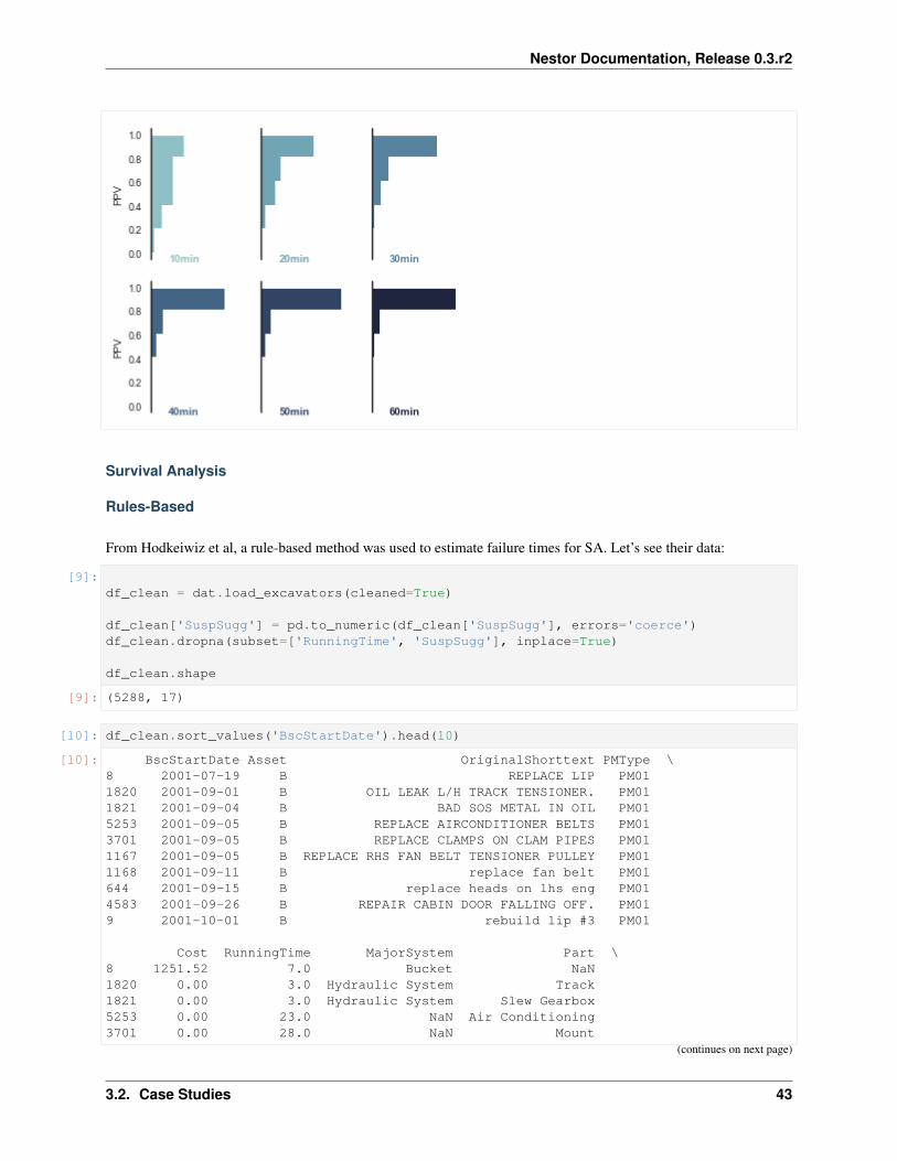
Convergence over time, using nestor-gui
As part of the comparison study, an expert used nestor-gui for approximately 60min annotating 1-grams, followedby 20min focusing on 2-grams. Work was saved every 10 min, so we would like to see how the above plot was arrivedat as the tokens were classified.
[10]: study_fname = Path('.')/'support'/'vocab_study_results.csv'study_df = pd.read_csv(study_fname, index_col=0)study_long = pd.melt(study_df, var_name="time", value_name='PPV').dropna()study_long['time_val'] = study_long.time.str.replace('min','').astype(float)
sns.set(style="white", rc={"axes.facecolor": (0, 0, 0, 0)}, context='paper')pal = sns.cubehelix_palette(6, rot=-.25, light=.7)g = sns.FacetGrid(study_long, col="time", hue="time", aspect=.8, height=2,→˓palette=pal, col_wrap=3)g.map(sns.distplot, "PPV", kde=False, bins=nbins, vertical=True,
hist_kws=dict(alpha=1., histtype='stepfilled', edgecolor='w', lw=2))g.map(plt.axvline, x=0, lw=1.4, clip_on=False, color='k')
# Define and use a simple function to label the plot in axes coordinatesdef label(x, color, label):
ax = plt.gca()ax.text(.2, 0, label, fontweight="bold", color=color,
ha="left", va="center", transform=ax.transAxes)g.map(label, "PPV")
# Remove axes details that don't play well with overlapg.set_titles("")g.set( xticks=[], xlabel='')g.set_axis_labels(y_var='PPV')g.despine(bottom=True, left=True)plt.tight_layout()
42 Chapter 3. Examples
Nestor Documentation, Release 0.3.r2
Survival Analysis
Rules-Based
From Hodkeiwiz et al, a rule-based method was used to estimate failure times for SA. Let’s see their data:
[9]:df_clean = dat.load_excavators(cleaned=True)
df_clean['SuspSugg'] = pd.to_numeric(df_clean['SuspSugg'], errors='coerce')df_clean.dropna(subset=['RunningTime', 'SuspSugg'], inplace=True)
df_clean.shape
[9]: (5288, 17)
[10]: df_clean.sort_values('BscStartDate').head(10)
[10]: BscStartDate Asset OriginalShorttext PMType \8 2001-07-19 B REPLACE LIP PM011820 2001-09-01 B OIL LEAK L/H TRACK TENSIONER. PM011821 2001-09-04 B BAD SOS METAL IN OIL PM015253 2001-09-05 B REPLACE AIRCONDITIONER BELTS PM013701 2001-09-05 B REPLACE CLAMPS ON CLAM PIPES PM011167 2001-09-05 B REPLACE RHS FAN BELT TENSIONER PULLEY PM011168 2001-09-11 B replace fan belt PM01644 2001-09-15 B replace heads on lhs eng PM014583 2001-09-26 B REPAIR CABIN DOOR FALLING OFF. PM019 2001-10-01 B rebuild lip #3 PM01
Cost RunningTime MajorSystem Part \8 1251.52 7.0 Bucket NaN1820 0.00 3.0 Hydraulic System Track1821 0.00 3.0 Hydraulic System Slew Gearbox5253 0.00 23.0 NaN Air Conditioning3701 0.00 28.0 NaN Mount
(continues on next page)
3.2. Case Studies 43

Nestor Documentation, Release 0.3.r2
(continued from previous page)
1167 82.09 0.0 NaN Fan1168 0.00 6.0 NaN Fan644 0.00 33.0 Engine NaN4583 0.00 27.0 NaN Drivers Cabin9 0.00 74.0 Bucket NaN
Action Variant FM Location Comments \8 Replace 2V NaN NaN NaN1820 Minor Maint 18 Leak Left NaN1821 NaN NaN Contamination NaN NaN5253 Replace 2V NaN NaN NaN3701 Replace 2V NaN NaN NaN1167 Minor Maint_Replace 2V NaN Right NaN1168 Replace 2V NaN NaN NaN644 Replace 2V NaN Left NaN4583 Repair 1 NaN NaN NaN9 Repair 5 NaN NaN NaN
FuncLocation SuspSugg \8 Bucket 0.01820 Power Train - Transmission 0.01821 Sprocket/Drive Compartment Right 0.05253 Air Conditioning System 0.03701 Oil - Hydraulic 0.01167 +Cooling System 0.01168 +Cooling System 0.0644 Engine Left Cylinder Heads 0.04583 Operators Cabin 0.09 Bucket Clam (Lip) 0.0
Rule Unnamed: 168 Rule_1_3_78_383_384 NaN1820 Rule_1_3_52_289_347_425_500 NaN1821 Rule_1_3_52_303_409 NaN5253 Rule_1_3_224_227_383_384 NaN3701 Rule_1_3_92_181_383_384 NaN1167 Rule_1_3_125_347_383_384_509 NaN1168 Rule_1_3_125_383_384 NaN644 Rule_1_3_25_383_384_499 NaN4583 Rule_1_3_251_284_357 NaN9 Rule_1_3_78_362 NaN
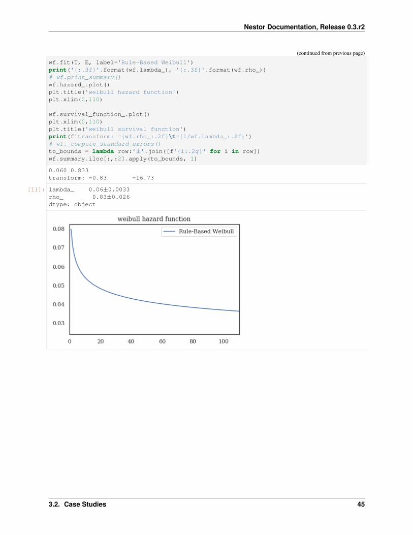
We once again turn to the library Lifelines as the work-horse for finding the Survival function.
[11]: from lifelines import WeibullFitter, ExponentialFitter, KaplanMeierFittermask = (df_clean.MajorSystem =='Bucket')# mask=df_clean.indexdef mask_to_ETclean(df_clean, mask, fill_null=1.):
filter_df = df_clean.loc[mask]g = filter_df.sort_values('BscStartDate').groupby('Asset')T = g['BscStartDate'].transform(pd.Series.diff).dt.days
# T.loc[(T<=0.)|(T.isna())] = fill_nullE = (~filter_df['SuspSugg'].astype(bool)).astype(int)return T.loc[~((T<=0.)|(T.isna()))], E.loc[~((T<=0.)|(T.isna()))]
T, E = mask_to_ETclean(df_clean, mask)wf = WeibullFitter()
(continues on next page)
44 Chapter 3. Examples
Nestor Documentation, Release 0.3.r2
(continued from previous page)
wf.fit(T, E, label='Rule-Based Weibull')print('{:.3f}'.format(wf.lambda_), '{:.3f}'.format(wf.rho_))# wf.print_summary()wf.hazard_.plot()plt.title('weibull hazard function')plt.xlim(0,110)
wf.survival_function_.plot()plt.xlim(0,110)plt.title('weibull survival function')print(f'transform: ={wf.rho_:.2f}\t={1/wf.lambda_:.2f}')# wf._compute_standard_errors()to_bounds = lambda row:'±'.join([f'{i:.2g}' for i in row])wf.summary.iloc[:,:2].apply(to_bounds, 1)
0.060 0.833transform: =0.83 =16.73
[11]: lambda_ 0.06±0.0033rho_ 0.83±0.026dtype: object
3.2. Case Studies 45

Nestor Documentation, Release 0.3.r2
Tag Based Comparison
We estimate the occurence of failures with tag occurrences.
[ ]: import math
def to_precision(x,p):"""returns a string representation of x formatted with a precision of p
Based on the webkit javascript implementation taken from here:https://code.google.com/p/webkit-mirror/source/browse/JavaScriptCore/kjs/number_
→˓object.cpp"""
x = float(x)
if x == 0.:return "0." + "0"*(p-1)
out = []
if x < 0:out.append("-")x = -x
e = int(math.log10(x))tens = math.pow(10, e - p + 1)n = math.floor(x/tens)
if n < math.pow(10, p - 1):e = e -1tens = math.pow(10, e - p+1)n = math.floor(x / tens)
(continues on next page)
46 Chapter 3. Examples

Nestor Documentation, Release 0.3.r2
(continued from previous page)
if abs((n + 1.) * tens - x) <= abs(n * tens -x):n = n + 1
if n >= math.pow(10,p):n = n / 10.e = e + 1
m = "%.*g" % (p, n)
if e < -2 or e >= p:out.append(m[0])if p > 1:
out.append(".")out.extend(m[1:p])
out.append('e')if e > 0:
out.append("+")out.append(str(e))
elif e == (p -1):out.append(m)
elif e >= 0:out.append(m[:e+1])if e+1 < len(m):
out.append(".")out.extend(m[e+1:])
else:out.append("0.")out.extend(["0"]*-(e+1))out.append(m)
return "".join(out)
[12]: def query_experiment(name, df, df_clean, rule, tag, multi_tag, prnt=False):
def mask_to_ETclean(df_clean, mask, fill_null=1.):filter_df = df_clean.loc[mask]g = filter_df.sort_values('BscStartDate').groupby('Asset')T = g['BscStartDate'].transform(pd.Series.diff).dt.daysE = (~filter_df['SuspSugg'].astype(bool)).astype(int)return T.loc[~((T<=0.)|(T.isna()))], E.loc[~((T<=0.)|(T.isna()))]
def mask_to_ETraw(df_clean, mask, fill_null=1.):filter_df = df_clean.loc[mask]g = filter_df.sort_values('BscStartDate').groupby('Asset')T = g['BscStartDate'].transform(pd.Series.diff).dt.daysT_defined = (T>0.)|T.notna()T = T[T_defined]# assume censored when parts replaced (changeout)E = (~(tag_df.S.changeout>0)).astype(int)[mask]E = E[T_defined]return T.loc[~((T<=0.)|(T.isna()))], E.loc[~((T<=0.)|(T.isna()))]
experiment = {'rules-based': {
'query': rule,'func': mask_to_ETclean,
(continues on next page)
3.2. Case Studies 47

Nestor Documentation, Release 0.3.r2
(continued from previous page)
'mask': (df_clean.MajorSystem == rule),'data': df_clean
},'single-tag': {
'query': tag,'func': mask_to_ETraw,'mask': tag_df.I[tag].sum(axis=1)>0,'data': df
},'multi-tag': {
'query': multi_tag,'func': mask_to_ETraw,'mask': tag_df.I[multi_tag].sum(axis=1)>0,'data': df
}}results = {
('query', 'text/tag'): [],# ('Weibull Params', r'$\lambda$'): [],
('Weibull Params', r'$\beta$'): [],('Weibull Params', '$\eta$'): [],('MTTF', 'Weib.'): [],('MTTF', 'K-M'): []}
idx = []
for key, info in experiment.items():idx += [key]results[('query','text/tag')] += [info['query']]if prnt:
print('{}: {}'.format(key, info['query']))info['T'], info['E'] = info['func'](info['data'], info['mask'])wf = WeibullFitter()wf.fit(info['T'], info['E'], label=f'{key} weibull')
to_bounds = lambda row:'$\pm$'.join([to_precision(row[0],2),to_precision(row[1],1)])
params = wf.summary.T.iloc[:2]params['eta_'] = [1/params.lambda_['coef'], # err. propagation
(params.lambda_['se(coef)']/params.lambda_['coef']**2)]params = params.T.apply(to_bounds, 1)
results[('Weibull Params', r'$\eta$')] += [params['eta_']]results[('Weibull Params', r'$\beta$')] += [params['rho_']]if prnt:
print('\tWeibull Params:\n','\t\t = {}\t'.format(params['eta_']),' = {}'.format(params['rho_']))
kmf = KaplanMeierFitter()kmf.fit(info["T"], event_observed=info['E'], label=f'{key} kaplan-meier')results[('MTTF','Weib.')] += [to_precision(wf.median_,3)]results[('MTTF','K-M')] += [to_precision(kmf.median_,3)]if prnt:
print(f'\tMTTF: \n\t\tWeib \t'+to_precision(wf.median_,3)+\'\n\t\tKM \t'+to_precision(kmf.median_,3))
(continues on next page)
48 Chapter 3. Examples

Nestor Documentation, Release 0.3.r2
(continued from previous page)
info['kmf'] = kmfinfo['wf'] = wf
return experiment, pd.DataFrame(results, index=pd.Index(idx, name=name))
[14]: bucket_exp, bucket_res = query_experiment('Bucket', df, df_clean,'Bucket',['bucket'],['bucket', 'tooth', 'lip', 'pin']);
[15]: tags = ['hyd', 'hose', 'pump', 'compressor']hyd_exp, hyd_res = query_experiment('Hydraulic System', df, df_clean,
'Hydraulic System',['hyd'],tags)
[16]: eng_exp, eng_res = query_experiment('Engine', df, df_clean,'Engine',['engine'],['engine', 'filter', 'fan'])
[17]: frames = [bucket_res, hyd_res, eng_res]res = pd.concat(frames, keys = [i.index.name for i in frames],
names=['Major System', 'method'])res
[17]: query Weibull Params \text/tag $\beta$
Major System methodBucket rules-based Bucket 0.83$\pm$0.03
single-tag [bucket] 0.83$\pm$0.03multi-tag [bucket, tooth, lip, pin] 0.82$\pm$0.02
Hydraulic System rules-based Hydraulic System 0.86$\pm$0.02single-tag [hyd] 0.89$\pm$0.04multi-tag [hyd, hose, pump, compressor] 0.89$\pm$0.02
Engine rules-based Engine 0.81$\pm$0.02single-tag [engine] 0.79$\pm$0.03multi-tag [engine, filter, fan] 0.81$\pm$0.02
MTTF$\eta$ Weib. K-M
Major System methodBucket rules-based 17$\pm$0.9 10.8 9.00
single-tag 27$\pm$2 17.1 15.0multi-tag 16$\pm$0.9 10.5 9.00
Hydraulic System rules-based 14$\pm$0.6 9.07 8.00single-tag 36$\pm$3 24.1 25.0multi-tag 15$\pm$0.7 9.74 9.00
Engine rules-based 17$\pm$1 10.8 9.00single-tag 19$\pm$1 11.8 10.0multi-tag 15$\pm$0.8 9.31 8.00
[18]:exp = [bucket_exp, eng_exp, hyd_exp]f,axes = plt.subplots(nrows=3, figsize=(5,10))
(continues on next page)
3.2. Case Studies 49

Nestor Documentation, Release 0.3.r2
(continued from previous page)
for n, ax in enumerate(axes):exp[n]['rules-based']['kmf'].plot(ax=ax, color='dodgerblue')exp[n]['multi-tag']['kmf'].plot(ax=ax, color='xkcd:rust', ls=':')exp[n]['single-tag']['kmf'].plot(ax=ax, color='xkcd:rust')
ax.set_xlim(0,110)ax.set_ylim(0,1)ax.set_title(r"$S(t)$"+f" of {res.index.levels[0][n]}")sns.despine()
plt.tight_layout()f.savefig('bkt_KMsurvival.png')
/home/tbsexton/anaconda3/lib/python3.6/site-packages/matplotlib/cbook/__init__.→˓py:2446: UserWarning: Saw kwargs [’c’, ’color’] which are all aliases for ’color’.→˓Kept value from ’color’seen=seen, canon=canonical, used=seen[-1]))
/home/tbsexton/anaconda3/lib/python3.6/site-packages/matplotlib/cbook/__init__.→˓py:2446: UserWarning: Saw kwargs [’c’, ’color’] which are all aliases for ’color’.→˓Kept value from ’color’seen=seen, canon=canonical, used=seen[-1]))
/home/tbsexton/anaconda3/lib/python3.6/site-packages/matplotlib/cbook/__init__.→˓py:2446: UserWarning: Saw kwargs [’c’, ’color’] which are all aliases for ’color’.→˓Kept value from ’color’seen=seen, canon=canonical, used=seen[-1]))
/home/tbsexton/anaconda3/lib/python3.6/site-packages/matplotlib/cbook/__init__.→˓py:2446: UserWarning: Saw kwargs [’c’, ’color’] which are all aliases for ’color’.→˓Kept value from ’color’seen=seen, canon=canonical, used=seen[-1]))
/home/tbsexton/anaconda3/lib/python3.6/site-packages/matplotlib/cbook/__init__.→˓py:2446: UserWarning: Saw kwargs [’c’, ’color’] which are all aliases for ’color’.→˓Kept value from ’color’seen=seen, canon=canonical, used=seen[-1]))
/home/tbsexton/anaconda3/lib/python3.6/site-packages/matplotlib/cbook/__init__.→˓py:2446: UserWarning: Saw kwargs [’c’, ’color’] which are all aliases for ’color’.→˓Kept value from ’color’seen=seen, canon=canonical, used=seen[-1]))
/home/tbsexton/anaconda3/lib/python3.6/site-packages/matplotlib/cbook/__init__.→˓py:2446: UserWarning: Saw kwargs [’c’, ’color’] which are all aliases for ’color’.→˓Kept value from ’color’seen=seen, canon=canonical, used=seen[-1]))
/home/tbsexton/anaconda3/lib/python3.6/site-packages/matplotlib/cbook/__init__.→˓py:2446: UserWarning: Saw kwargs [’c’, ’color’] which are all aliases for ’color’.→˓Kept value from ’color’seen=seen, canon=canonical, used=seen[-1]))
/home/tbsexton/anaconda3/lib/python3.6/site-packages/matplotlib/cbook/__init__.→˓py:2446: UserWarning: Saw kwargs [’c’, ’color’] which are all aliases for ’color’.→˓Kept value from ’color’seen=seen, canon=canonical, used=seen[-1]))
50 Chapter 3. Examples

Nestor Documentation, Release 0.3.r2
This next one give you an idea of the differences better. using a log-transform. the tags under-estimate death ratesa little in the 80-130 day range, probably because there’s a failure mode not captured by the [bucket, lip, tooth] tags(because it’s rare).
[20]: f,axes = plt.subplots(nrows=3, figsize=(5,10))for n, ax in enumerate(axes):
exp[n]['rules-based']['kmf'].plot_loglogs(ax=ax, c='dodgerblue')
(continues on next page)
3.2. Case Studies 51

Nestor Documentation, Release 0.3.r2
(continued from previous page)
exp[n]['single-tag']['kmf'].plot_loglogs(ax=ax, c='xkcd:rust', ls=':')exp[n]['multi-tag']['kmf'].plot_loglogs(ax=ax, c='xkcd:rust')if n != 2:
ax.legend_.remove()# ax.set_xlim(0,110)# ax.set_ylim(0,1)
ax.set_title(r"$\log(-\log(S(t)))$"+f" of {res.index.levels[0][n]}")sns.despine()
plt.tight_layout()f.savefig('bkt_logKMsurvival.png', dpi=300)# kmf.plot_loglogs()
52 Chapter 3. Examples

Nestor Documentation, Release 0.3.r2
[ ]:
[1]: from pathlib import Pathimport numpy as npimport pandas as pdimport seaborn as snsimport matplotlib.pyplot as plt
(continues on next page)
3.2. Case Studies 53

Nestor Documentation, Release 0.3.r2
(continued from previous page)
%matplotlib inline
[2]: def set_style():# This sets reasonable defaults for font size for a figure that will go in a papersns.set_context("paper")# Set the font to be serif, rather than sanssns.set(font='serif')# Make the background white, and specify the specific font familysns.set_style("white", {
"font.family": "serif","font.serif": ["Times", "Palatino", "serif"]
})set_style()
3.2.3 HVAC Maintenance Case Study
Import Data
[3]: import nestor.keyword as kexdata_dir = Path('../..')/'data'/'hvac_data'df = pd.read_csv(data_dir/'hvac_data.csv')# really important things we know, a priorispecial_replace={'action taken': '',
' -': '; ','- ': '; ','too hot': 'too_hot','to hot': 'too_hot','too cold': 'too_cold','to cold': 'too_cold'}
nlp_select = kex.NLPSelect(columns = ['DESCRIPTION', 'LONG_DESCRIPTION'], special_→˓replace=special_replace)raw_text = nlp_select.transform(df)
/home/tbsexton/anaconda3/envs/nestor-dev/lib/python3.6/site-packages/IPython/core/→˓interactiveshell.py:3020: DtypeWarning: Columns (29,30,40,106,172,196,217,227) have→˓mixed types. Specify dtype option on import or set low_memory=False.interactivity=interactivity, compiler=compiler, result=result)
Build Vocab
[4]:tex = kex.TokenExtractor()toks = tex.fit_transform(raw_text)print(tex.vocab_)
[’room’ ’poc’ ’stat’ ... ’llines’ ’pictures’ ’logged’]
[5]: vocab_fname = data_dir/'vocab.csv'# vocab_fname = data_dir/'mine_vocab_app.csv'
(continues on next page)
54 Chapter 3. Examples

Nestor Documentation, Release 0.3.r2
(continued from previous page)
# vocab = tex.annotation_assistant(filename = vocab_fname)vocab = kex.generate_vocabulary_df(tex, init = vocab_fname)
intialized successfully!
Extract Keywords
[6]: tag_df = kex.tag_extractor(tex, raw_text, vocab_df=vocab)tags_read = kex._get_readable_tag_df(tag_df)
intialized successfully!
HBox(children=(IntProgress(value=0, description='Category Loop', max=6,→˓style=ProgressStyle(description_width=...
HBox(children=(IntProgress(value=0, description='I token loop', max=45,→˓style=ProgressStyle(description_width=...
HBox(children=(IntProgress(value=0, description='NA token loop', max=4668,→˓style=ProgressStyle(description_wid...
HBox(children=(IntProgress(value=0, description='P token loop', max=7,→˓style=ProgressStyle(description_width='...
HBox(children=(IntProgress(value=0, description='S token loop', max=16,→˓style=ProgressStyle(description_width=...
HBox(children=(IntProgress(value=0, description='U token loop', max=14,→˓style=ProgressStyle(description_width=...
HBox(children=(IntProgress(value=0, description='X token loop', max=3,→˓style=ProgressStyle(description_width='...
[7]: tags_read.head(5)
[7]: I NA P \0 pm, order, site, aml, charge1 time pm, cover, order, aml, charge, charged2 point_of_contact, thermostat ed3 point_of_contact, thermostat ed4 thermostat
S U X0 complete1 need2 replace, adjust, reset, repair freeze3 adjust, reset, repair, restart freeze4 adjust, reset, repair freeze
[8]:# vocab = pd.read_csv(data_dir/'app_vocab_mike.csv', index_col=0)# how many instances of each keyword class are there?print('named entities: ')print('I\tItem\nP\tProblem\nS\tSolution\nR\tRedundant')print('U\tUnknown\nX\tStop Word')
(continues on next page)
3.2. Case Studies 55
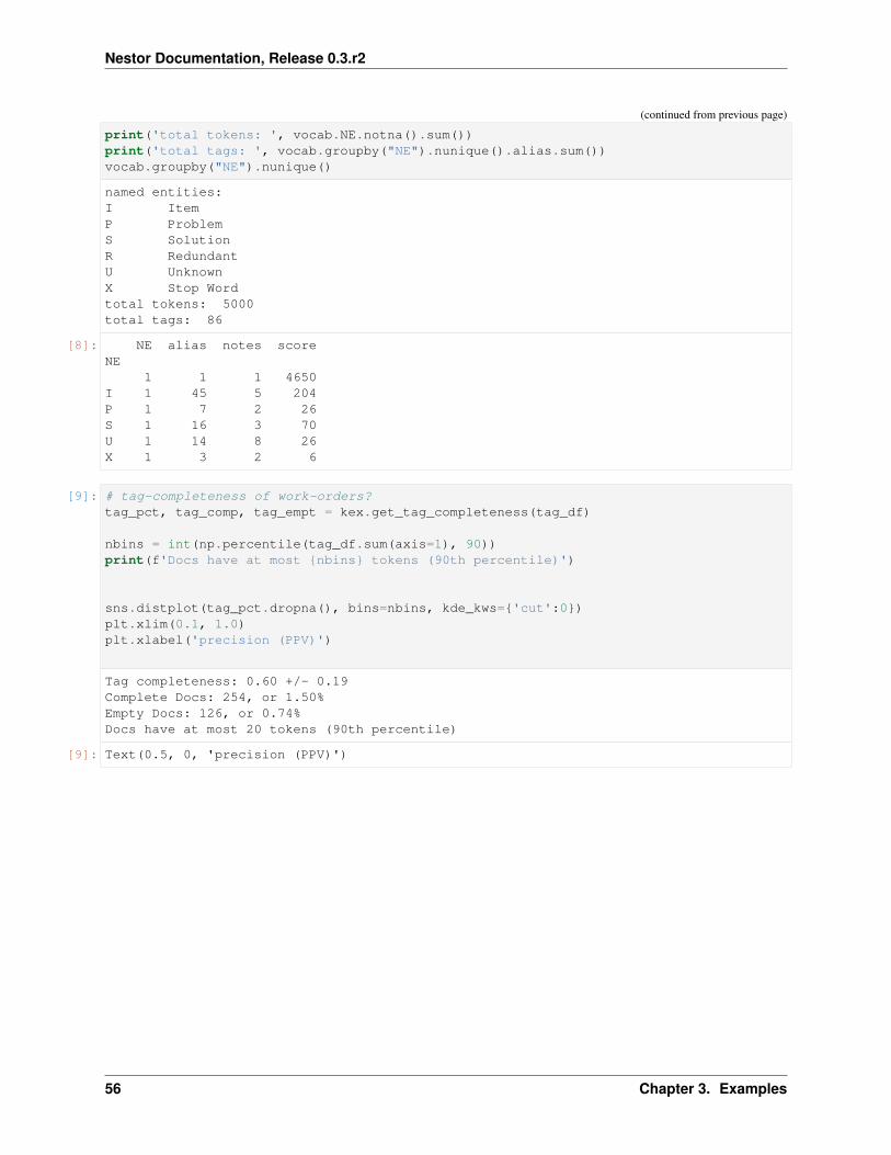
Nestor Documentation, Release 0.3.r2
(continued from previous page)
print('total tokens: ', vocab.NE.notna().sum())print('total tags: ', vocab.groupby("NE").nunique().alias.sum())vocab.groupby("NE").nunique()
named entities:I ItemP ProblemS SolutionR RedundantU UnknownX Stop Wordtotal tokens: 5000total tags: 86
[8]: NE alias notes scoreNE
1 1 1 4650I 1 45 5 204P 1 7 2 26S 1 16 3 70U 1 14 8 26X 1 3 2 6
[9]: # tag-completeness of work-orders?tag_pct, tag_comp, tag_empt = kex.get_tag_completeness(tag_df)
nbins = int(np.percentile(tag_df.sum(axis=1), 90))print(f'Docs have at most {nbins} tokens (90th percentile)')
sns.distplot(tag_pct.dropna(), bins=nbins, kde_kws={'cut':0})plt.xlim(0.1, 1.0)plt.xlabel('precision (PPV)')
Tag completeness: 0.60 +/- 0.19Complete Docs: 254, or 1.50%Empty Docs: 126, or 0.74%Docs have at most 20 tokens (90th percentile)
[9]: Text(0.5, 0, 'precision (PPV)')
56 Chapter 3. Examples

Nestor Documentation, Release 0.3.r2
Measuring Machine Performance
[10]: import nestor.tagplots as tagpltsamp = ['air_conditioning_unit','fan', 'valve', 'leak', 'too_hot', 'too_cold']cond = (tag_df.P.alarm==1)sample_tag = tag_df.loc[:,(slice(None), samp)]sample_tag.columns = sample_tag.columns.droplevel(0)
idx_col = pd.DatetimeIndex(df.REPORTDATE)sample_tag = sample_tag.set_index(idx_col[:])sample_tag = sample_tag[ sample_tag.index.year.isin([2009, 2010, 2016])]
tagplt.tagcalendarplot(sample_tag,how='sum', fig_kws={'figsize':(13,8)});
plt.suptitle('Tag Occurence')
[10]: Text(0.5, 0.98, 'Tag Occurence')
3.2. Case Studies 57

Nestor Documentation, Release 0.3.r2
Monthly “too-hot” and “too-cold” requests, over time
[18]: import holoviews as hvimport geoviews as gvhv.extension('bokeh')
Data type cannot be displayed: application/javascript, application/vnd.holoviews_load.v0+json
Data type cannot be displayed: application/javascript, application/vnd.holoviews_load.v0+json
[146]: %%output size=200temp_curve_spec = {# 'Spread':{'plot':{'width':300, 'height':80},# 'style':dict(line_color=None, alpha=.4, color=hv.Cycle(['#fe420f', '→˓#06b1c4']))},
'Curve':{'plot':{'width':300, 'height':80}},'Curve.TooHot':{'style':dict(color='#fe420f')},'Curve.TooCold':{'style':dict(color='#06b1c4')},'NdOverlay': {'plot':dict(title='Requests')}
}# 'Scatter':{'style':dict( size=5, color=hv.Cycle(['#fe420f', '#06b1c4']))}
# hv.Cycle(['#fe420f', '#06b1c4'])
samp = ['too_cold', 'too_hot']
(continues on next page)
58 Chapter 3. Examples

Nestor Documentation, Release 0.3.r2
(continued from previous page)
sample_tag = tag_df.loc[:,(slice(None), samp)]sample_tag.columns = sample_tag.columns.droplevel(0)
sample_tag = sample_tag.set_index(idx_col).sort_index()
# resamp = '30D'resamp = '1W'meas = sample_tag[pd.datetime(2009,9,1):pd.datetime(2012,3,1)].resample(resamp).sum()meas['date'] = meas.index# roll = sample_tag.rolling('10D').mean()# mean = sample_tag.rolling('1D').mean().resample(resamp).sum()# err = sample_tag.rolling('1D').std().resample(resamp).sum()
# temp_curves = hv.Overlay([# # hv.Spread((mean.index, mean.too_hot, err.too_hot)),# # hv.Spread((mean.index, mean.too_cold, err.too_cold)),# hv.Curve((meas.index, meas.too_hot)),# hv.Curve((meas.index, meas.too_cold)),# # hv.Scatter((meas.index, meas.too_hot), label='too_hot'),# # hv.Scatter((meas.index, meas.too_cold), label='too_cold')# ])
# table = hv.Table(meas, ['too_hot', 'too_cold'], 'date')temp_curves = hv.NdOverlay({
'too_cold':hv.Curve(meas,'date', 'too_cold', group='Requests', name='TooCold'),'too_hot':hv.Curve(meas, 'date','too_hot', group='Requests', name='TooHot'),
}).opts(temp_curve_spec)# temp_curves.select().opts(temp_curve_spec)#*hv.VLine(times[5])# hv.Curve(table)
# temp_curves.select(date=(pd.datetime(2010,1,1),pd.datetime(2012,1,1)))# temp_curves.select(too_hot=(meas.too_hot.quantile(.25),meas.too_hot.quantile(.75)))
# meas[pd.datetime(2010,1,1):pd.datetime(2012,1,1)]temp_curves
[146]: :NdOverlay [Element]:Curve [date] (too_hot)
[147]: pd.datetime(2010, 1, 1)
[147]: datetime.datetime(2010, 1, 1, 0, 0)
[148]: import geopandas as gpdnist_df = gpd.read_file(str(data_dir/'nist_map.geojson')).set_index('bldg',→˓drop=False)nist_df.index = nist_df.index.astype(str)samp = ['too_cold', 'too_hot']sample_tag = tag_df.loc[:,(slice(None), samp)]sample_tag.columns = sample_tag.columns.droplevel(0)
bldg_col = df.LOCATION.str.split('-').str[0].astype('category')sample_tag = pd.concat([sample_tag, bldg_col], axis=1)sample_tag = sample_tag.set_index(idx_col).sort_index()sample_tag.rename({'LOCATION':'bldg'}, axis='columns', inplace=True)
times = sample_tag.loc['2010-1-1':'2012-1-1'].resample('1QS').sum().index
(continues on next page)
3.2. Case Studies 59

Nestor Documentation, Release 0.3.r2
(continued from previous page)
# pd.concat([sample_tag.loc[times[0]:times[1]].groupby('bldg').sum(), nist_df],→˓axis=1).dropna()
def get_bldg_temp(n):data = gpd.GeoDataFrame(pd.concat([sample_tag.loc[times[n]:times[n+1]].groupby(
→˓'bldg').sum(),nist_df],
axis=1).dropna())data['Temperature Index'] = np.tanh((data['too_cold'].sum()+data['too_hot'].
→˓sum())/20)*\(data['too_cold'] - data['too_hot'])return data
# np.tanh((data['too_cold'].sum()+data['too_hot'].sum())/20)*\get_bldg_temp(1).head()
[148]: too_hot too_cold bldg \bldg101 34 14 101.0202 4 2 202.0203 0 0 203.0205 0 0 205.0215 0 0 215.0
geometry Temperature Indexbldg101 POLYGON ((-77.2163987159729 39.13512015465694,... -20.0202 POLYGON ((-77.22025036811827 39.13047428646352... -2.0203 POLYGON ((-77.22077608108521 39.13020796677279... 0.0205 POLYGON ((-77.21850156784058 39.1223198699503,... 0.0215 POLYGON ((-77.21671521663666 39.1316623096919,... 0.0
[149]: from bokeh.palettes import Viridis10, Category10_6, RdBu10from bokeh.models.mappers import LinearColorMapperRdBu10.reverse()padding = dict(x=(-77.223, -77.214), y=(39.13, 39.14))extents = (-77.223, 39.129, -77.214, 39.1385)
bldg_dict, vlines = {}, {}for n, time in enumerate(times[:-1]):
mapped = gv.Polygons(get_bldg_temp(n),vdims=['Temperature Index', 'bldg', 'too_hot', 'too_cold'],extents = extents)
mapped = mapped.redim.range(**padding)vlines[time] = hv.VLine(time).opts(style={'color':'black'})bldg_dict[time] = mapped
text = hv.Overlay([gv.Text(i.centroid.x-.0002,i.centroid.y-.00015,str(name)) for name,i in get_bldg_temp(0).geometry.
→˓iteritems()])
[150]: %%output size=200 filename='nist_hvac_map'%%opts Polygons [height=350 width=300, tools=['hover'] colorbar=False ] (cmap='RdBu')%%opts VLine (alpha=.5)
(continues on next page)
60 Chapter 3. Examples

Nestor Documentation, Release 0.3.r2
(continued from previous page)
import warningswarnings.simplefilter(action='ignore', category=FutureWarning)
(hv.HoloMap(bldg_dict, 'Time')*text +\hv.HoloMap(vlines, 'Time')*\temp_curves.opts(temp_curve_spec)).cols(1)
# hv.Bounds()
[150]: :Layout.HoloMap.I :HoloMap [Time]
:Overlay.Polygons.I :Polygons [Longitude,Latitude] (Temperature Index,bldg,too_
→˓hot,too_cold).Text.I :Text [x,y].Text.II :Text [x,y].Text.III :Text [x,y].Text.IV :Text [x,y].Text.V :Text [x,y].Text.VI :Text [x,y].Text.VII :Text [x,y].Text.VIII :Text [x,y].Text.IX :Text [x,y].Text.X :Text [x,y].Text.XI :Text [x,y].Text.XII :Text [x,y].Text.XIII :Text [x,y].Text.XIV :Text [x,y].Text.XV :Text [x,y].Text.XVI :Text [x,y].Text.XVII :Text [x,y].Text.XVIII :Text [x,y].Text.XIX :Text [x,y].Text.XX :Text [x,y].Text.XXI :Text [x,y].Text.XXII :Text [x,y].Text.XXIII :Text [x,y].Text.XXIV :Text [x,y].Text.XXV :Text [x,y].Text.XXVI :Text [x,y].Text.XXVII :Text [x,y].Text.XXVIII :Text [x,y].Text.XXIX :Text [x,y].Text.XXX :Text [x,y]
.Requests.I :HoloMap [Time]:Overlay
.VLine.I :VLine [x,y]
.Requests.I :NdOverlay [Element]:Curve [date] (too_hot)
[ ]:
3.2. Case Studies 61

Nestor Documentation, Release 0.3.r2
62 Chapter 3. Examples

CHAPTER
FOUR
ADVANCED USE
These features/applications are intended for contributors or collaborators, comfortable dealing with bugs/incompleteprojects.
4.1 Research Mode
4.1.1 Setup
• If you have not already done so, install the Nestor app according to the instructions.
• If you have not used Nestor before, read these instructions and get familiar with the tool.
4.1.2 Study Task
1. Launch Nestor. Select “Research Mode -> New Project” in the top menu bar.
#. Check each of the four checkboxes in the “How do you want the tool to save your changes?” section. In the authorfield, enter your name or a nickname to differentiate your data from the other study participants. Click “OK.” #.
Use the “Single Word Analysis” tab to tag for approximately 30 minutes:
1. Select the word
2. Select similar words
#. Create an alias #.
Choose a classification
At this stage you may take a break if desired before proceeding to the next step.
1. Select “Auto-populate” in the top menu and select “Multi-Word from Single Word Vocabulary”
2. Select the “Multi word analysis” tab and tag for approximately 30 minutes:
1. Check the auto populated words (they will have classifications already selected in the classification col-umn)
1. Check if the classification is correct
2. Check if the alias is correct
3. If yes, hit next word. If no, modify as necessary.
2. Once auto populated words are checked, move on to other words and create classification and aliases
3. Go to “Report” tab and hit “Update Tag Extraction”
63

Nestor Documentation, Release 0.3.r2
4. Select “Create new csv” and save
TODO Share file
64 Chapter 4. Advanced Use
CHAPTER
FIVE
NESTOR PACKAGE
Quantifying tacit knowledge investigatory analysis
Nestor is a toolkit for using Natural Language Processing (NLP) with efficient user-interaction to perform structureddata extraction with minimal annotation time-cost.
5.1 Subpackages
5.1.1 nestor.datasets package
load_excavators(cleaned=False)Helper function to load excavator toy dataset.
Hodkiewicz, M., and Ho, M. (2016) “Cleaning historical maintenance work order data for reliability analysis”in Journal of Quality in Maintenance Engineering, Vol 22 (2), pp. 146-163.
Parameters cleaned (bool (default=False)) – whether to return the original dataset (False) or thedataset with keyword extraction rules applied (True), as described in Hodkiewicz and Ho (2016)
Returns
pandas.DataFrame –
BscStartDate : initialization of MWO
Asset : which excavator this MWO concerns (A, B, C, D, E)
OriginalShorttext : natural language description of the MWO
PMType : repair (PM01) or replacement (PM02)
Cost : MWO expense (AUD)
5.2 Submodules
5.2.1 nestor.keyword module
author: Thurston Sexton
class NLPSelect(columns=0, special_replace=None)Bases: nestor.keyword.Transformer
Extract specified natural language columns from a pd.DataFrame, and combine into a single series.
65

Nestor Documentation, Release 0.3.r2
Parameters columns (int, or list of int or str.) – corresponding columns in X to extract, clean, andmerge
get_params(self, deep=True)
transform(self, X, y=None)
class TokenExtractor(**tfidf_kwargs)Bases: sklearn.base.TransformerMixin
A wrapper for the sklearn TfidfVectorizer class, with utilities for ranking by total tf-idf score, and getting a listof vocabulary.
Parameters
• tfidf_kwargs (arguments to pass to sklearn’s TfidfVectorizer)
• Valid options modified here (see sklearn docs for more options) are –
input [string {‘filename’, ‘file’, ‘content’}, default=’content’] If ‘filename’, the sequencepassed as an argument to fit is expected to be a list of filenames that need reading to fetchthe raw content to analyze.
If ‘file’, the sequence items must have a ‘read’ method (file-like object) that is called tofetch the bytes in memory.
Otherwise the input is expected to be the sequence strings or bytes items are expected tobe analyzed directly.
ngram_range [tuple (min_n, max_n), default=(1,1)] The lower and upper boundary of therange of n-values for different n-grams to be extracted. All values of n such that min_n<= n <= max_n will be used.
stop_words [string {‘english’} (default), list, or None] If a string, it is passed to_check_stop_list and the appropriate stop list is returned. ‘english’ is currently the onlysupported string value.
If a list, that list is assumed to contain stop words, all of which will be removed from theresulting tokens. Only applies if analyzer == 'word'.
If None, no stop words will be used. max_df can be set to a value in the range [0.7, 1.0)to automatically detect and filter stop words based on intra corpus document frequency ofterms.
max_features [int or None, default=5000] If not None, build a vocabulary that only con-sider the top max_features ordered by term frequency across the corpus.
This parameter is ignored if vocabulary is not None.
smooth_idf [boolean, default=False] Smooth idf weights by adding one to document fre-quencies, as if an extra document was seen containing every term in the collection exactlyonce. Prevents zero divisions.
sublinear_tf [boolean, default=True] Apply sublinear tf scaling, i.e. replace tf with 1 +log(tf).
fit(self, X, y=None)
fit_transform(self, X, y=None, **fit_params)Fit to data, then transform it.
Fits transformer to X and y with optional parameters fit_params and returns a transformed version of X.
Parameters
66 Chapter 5. nestor package

Nestor Documentation, Release 0.3.r2
• X (numpy array of shape [n_samples, n_features]) – Training set.
• y (numpy array of shape [n_samples]) – Target values.
Returns X_new (numpy array of shape [n_samples, n_features_new]) – Transformed array.
ranks_Retrieve the rank of each token, for sorting. Uses summed scoring over the TF-IDF for each token, so that:𝑆𝑡 =MWO TF-IDF𝑡
Returns ranks (numpy.array)
scores_Returns actual scores of tokens, for progress-tracking (unit-normalized)
Returns numpy.array
transform(self, dask_documents, copy=True)
vocab_ordered list of tokens, rank-ordered by summed-tf-idf (see ranks_())
Returns extracted_toks (numpy.array)
generate_vocabulary_df(transformer, filename=None, init=None)Helper method to create a formatted pandas.DataFrame and/or a .csv containing the to-ken–tag/alias–classification relationship. Formatted as jargon/slang tokens, the Named Entity classifications,preferred labels, notes, and tf-idf summed scores:
tokens | NE | alias | notes | scores
This is intended to be filled out in excel or using the Tagging Tool.
Parameters
• transformer (object TokenExtractor) – the (TRAINED) token extractor used to generatethe ranked list of vocab.
• filename (str, optional) – the file location to read/write a csv containing a formatted vocab-ulary list
• init (str or pd.Dataframe, optional) – file location of csv or dataframe of existing vocab listto read and update token classification values from
Returns vocab (pd.Dataframe) – the correctly formatted vocabulary list for token:NE, alias match-ing
get_tag_completeness(tag_df)
Parameters tag_df (pd.DataFrame) – heirarchical-column df containing
tag_extractor(transformer, raw_text, vocab_df=None, readable=False)Wrapper for the TokenExtractor to streamline the generation of tags from text. Determines the documents in<raw_text> that contain each of the tags in <vocab>, using a TokenExtractor transformer object (i.e. the tfidfvocabulary).
As implemented, this function expects an existing transformer object, though in the future this will be changedto a class-like functionality (e.g. sklearn’s AdaBoostClassifier, etc) which wraps a transformer into a new one.
Parameters
• transformer (object KeywordExtractor) – instantiated, can be pre-trained
• raw_text (pd.Series) – contains jargon/slang-filled raw text to be tagged
5.2. Submodules 67

Nestor Documentation, Release 0.3.r2
• vocab_df (pd.DataFrame, optional) – An existing vocabulary dataframe or .csv filename,expected in the format of kex.generate_vocabulary_df().
• readable (bool, default False) – whether to return readable, categorized, comma-sep strformat (takes longer)
Returns
• pd.DataFrame, extracted tags for each document, whether binary indicator (default)
• or in readable, categorized, comma-sep str format (readable=True, takes longer)
token_to_alias(raw_text, vocab)Replaces known tokens with their “tag” form, i.e. the alias’ in some known vocabulary list
Parameters
• raw_text (pd.Series) – contains text with known jargon, slang, etc
• vocab (pd.DataFrame) – contains alias’ keyed on known slang, jargon, etc.
Returns pd.Series – new text, with all slang/jargon replaced with unified representations
ngram_automatch(voc1, voc2, NE_types=None, NE_map_rules=None)Experimental method to auto-match tag combinations into higher-level concepts, for user-suggestion. Used innestor.ui
5.2.2 nestor.tagplots module
author: Thurston Sexton
class TagPlot(data_file, cat_specifier=’name’, topn=10)Bases: object
Central holder for holoviews dynamic-maps, to be served as a Bokeh App.
filter_tags(self, obj_type, obj_name, n_thres=20)apply filter to binary tag matrix (tag_df) :Parameters: * obj_type (passed to filter_type_name)
• obj_name (passed to filter_type_name)
• n_thres (only return nodes in the top n_thres percentile)
Returns pd.DataFrame, filtered binary tax matrix
filter_type_name(self, obj_type, obj_name)build a mask to filter data on :Parameters: * obj_type (class of object to filter on)
• obj_name (sub-class/instance to filter on)
Returns pd.Series, mask for filtering df, tag_df.
hv_bars(self, obj_type)Generates a hv.DynamicMap with a bars/frequency representation of filtered tags. :Parameters: obj_type(class of object to show)
Returns hv.DynamicMap
hv_flow(self, obj_type)Generates a hv.DynamicMap with a Sankey/flow representation of filtered tags. :Parameters: obj_type(class of object to show)
Returns hv.DynamicMap
68 Chapter 5. nestor package

Nestor Documentation, Release 0.3.r2
hv_nodelink(self, obj_type)Generates a hv.DynamicMap with a nodelink representation of filtered tags. :Parameters: obj_type (classof object to show)
Returns hv.DynamicMap
tag_relation_net(tag_df, name=None, kind=’coocc’, layout=<function fruchterman_reingold_layoutat 0x7f2703770378>, layout_kws=None, padding=None, **node_adj_kws)
Explore tag relationships by create a Holoviews Graph Element. Nodes are tags (colored by classification), andedges occur only when those tags happen together.
Parameters
• tag_df (pandas.DataFrame) – standard Nestor tag occurrence matrix. Multi-column withtop-level containing tag classifications (named-entity NE) and 2nd level containing tags.Each row corresponds to a single event (MWO), with binary indicators (1-occurs, 0-doesnot).
• name (str) – what to name this tag relation element. Creates a Holoviews group “name”.
• kind (str) –
coocc : co-occurrence graph, where tags are connected if they occur in the same MWO,above the value calculated for pct_thres. Connects all types together.
sankey : Directed “flow” graph, currently implemented with a (P) -> (I) -> (S) structure.Will require dag=True. Alters default to similarity=count
• layout (object (function), optional) – must take a graph object as input and output 2D co-ordinates for node locations (e.g. all networkx.layout functions). Defaults to networkx.spring_layout
• layout_kws (dict, optional) – options to pass to networkx layout functions
• padding (dict, optional) –
contains “x” and “y” specifications for boundaries. Defaults: {'x':(-0.05, 1.05), 'y':(-0.05, 1.05)}
Only valid if kind is ‘coocc’.
• node_adj_kws –
keyword arguments for nestor.tagtrees.tag_df_network. Valid options aresimilarity : ‘cosine’ (default) or ‘count’ dag : bool, default=’False’, (True ifkind='sankey') pct_thres : : int or None
If int, between [0,100]. The lower percentile at which to threshold edges/adjacency.
Returns graph (holoviews.Holomap or holoviews.Graph element, pending sankey or cooccurrenceinput.)
tagcalendarplot(tag_df, how=’sum’, yearlabels=True, yearascending=True, yearlabel_kws=None, sub-plot_kws=None, gridspec_kws=None, fig_kws=None, **kwargs)
Plot a timeseries of (binary) tag occurrences as a calendar heatmap over weeks in the year. any columns passedwill be explicitly plotted as rows, with each week in the year as a column. By default, occurences are summed,not averaged, but this aggregation over weeks may be any valid option for the pandas.Dataframe.agg() method.
This function will separate out multiple years within the data as multiple calendars. The plotting has beenheavily modified/altered/normalized, but the original version appeared here:
adapted from: ‘Martijn Vermaat’ 14 Feb 2016 ‘[email protected]’ ‘https://github.com/martijnvermaat/calmap’
5.2. Submodules 69

Nestor Documentation, Release 0.3.r2
Parameters
• tag_df (pandas.DataFrame) – standard Nestor tag occurrence matrix. Multi-column withtop-level containing tag classifications (named-entity NE) and 2nd level containing tags.Each row corresponds to a single event (MWO), with binary indicators (1-occurs, 0-doesnot).
• how (string) – Method for resampling data by day. If None, assume data is already sampledby day and don’t resample. Otherwise, this is passed to Pandas Series.resample.
• yearlabels (bool) – Whether or not to draw the year for each subplot.
• yearascending (bool) – Sort the calendar in ascending or descending order.
• yearlabel_kws (dict) – Keyword arguments passed to the matplotlib set_ylabel call whichis used to draw the year for each subplot.
• subplot_kws (dict) – Keyword arguments passed to the matplotlib add_subplot call used tocreate each subplot.
• gridspec_kws (dict) – Keyword arguments passed to the matplotlib GridSpec constructorused to create the grid the subplots are placed on.
• fig_kws (dict) – Keyword arguments passed to the matplotlib figure call.
• kwargs (other keyword arguments) – All other keyword arguments are passed to yearplot.
Returns fig, axes (matplotlib Figure and Axes) – Tuple where fig is the matplotlib Figure objectaxes is an array of matplotlib Axes objects with the calendar heatmaps, one per year.
tagyearplot(tag_df, year=None, how=’sum’, vmin=None, vmax=None, cmap=’Reds’, linewidth=1, line-color=None, monthlabels=[’Jan’, ’Feb’, ’Mar’, ’Apr’, ’May’, ’Jun’, ’Jul’, ’Aug’, ’Sep’, ’Oct’,’Nov’, ’Dec’], monthticks=True, ax=None, **kwargs)
Plot a timeseries of (binary) tag occurrences as a calendar heatmap over weeks in the year. any columns passedwill be explicitly plotted as rows, with each week in the year as a column. By default, occurences are summed,not averaged, but this aggregation over weeks may be any valid option for the pandas.Dataframe.agg() method.
adapted from: ‘Martijn Vermaat’ 14 Feb 2016 ‘[email protected]’ ‘https://github.com/martijnvermaat/calmap’
Parameters
• tag_df (pandas.DataFrame) – standard Nestor tag occurrence matrix. Multi-column withtop-level containing tag classifications (named-entity NE) and 2nd level containing tags.Each row corresponds to a single event (MWO), with binary indicators (1-occurs, 0-doesnot).
• year (integer) – Only data indexed by this year will be plotted. If None, the first year forwhich there is data will be plotted.
• how (string) – Method for resampling data by day. If None, assume data is already sampledby day and don’t resample. Otherwise, this is passed to Pandas Series.resample.
• vmin, vmax (floats) – Values to anchor the colormap. If None, min and max are used afterresampling data by day.
• cmap (matplotlib colormap name or object) – The mapping from data values to color space.
• linewidth (float) – Width of the lines that will divide each day.
• linecolor (color) – Color of the lines that will divide each day. If None, the axes backgroundcolor is used, or ‘white’ if it is transparent.
• monthlabels (list) – Strings to use as labels for months, must be of length 12.
70 Chapter 5. nestor package

Nestor Documentation, Release 0.3.r2
• monthticks (list or int or bool) – If True, label all months. If False, don’t label months. Ifa list, only label months with these indices. If an integer, label every n month.
• ax (matplotlib Axes) – Axes in which to draw the plot, otherwise use the currently-activeAxes.
• kwargs (other keyword arguments) – All other keyword arguments are passed to matplotlibax.pcolormesh.
Returns ax (matplotlib Axes) – Axes object with the calendar heatmap.
5.2.3 nestor.tagtrees module
__author__ = “Thurston Sexton”
get_onehot(df, col, topn=700)DEPRECATED!
get_relevant(df, col, topn=20)DEPRECATED!
Parameters
• df (a dataframe containing columns of tag assignments (comma-sep, str))
• col (which column to extract)
• topn (how many of the top most frequent tags to return)
Returns list of (tag,count,numpy.array) tuples
heymann_taxonomy(dist_mat, cent_prog=’pr’, tau=0.0005, dynamic=False, dotfile=None, ver-bose=False)
Parameters
• dist_mat (pandas.DataFrame) – contains similarity matrix, indexed and named by tags
• cent_prog (str) – algorithm to use in calculating node centrality
pr: PageRank eig: eigencentrality btw: betweenness cls: closeness
• tau (float) – similarity threshold for retaining a node
• dynamic (bool) – whether to re-calculate centrality after popping every tag
• write_dot (str or None) – file location, where to save a .dot, if any.
• verbose (bool) – print some stuff
node_adj_mat(tag_df, similarity=’cosine’, dag=False, pct_thres=None)Calculate the similarity of tags, in the form of a similarity kernel. Used as input to graph/network methods.
Parameters
• tag_df (pandas.DataFrame) – standard Nestor tag occurrence matrix. Multi-column withtop-level containing tag classifications (named-entity NE) and 2nd level containing tags.Each row corresponds to a single event (MWO), with binary indicators (1-occurs, 0-doesnot).
• similarity (str) – cosine: cosine similarity (from sklearn.metrix.pairwise) count:count (the number of co-occurrences of each tag-tag pair)
5.2. Submodules 71

Nestor Documentation, Release 0.3.r2
• dag (bool) – default adj_mat will be accross all nodes. This option will return a directed,acyclic graph (DAG), useful for things like Sankey Diagrams. Current implementation re-turns (P) -> (I) -> (S) structure (deletes others).
• pct_thres (int or None) – If int, between [0,100]. The lower percentile at which to thresholdedges/adjacency.
Returns pandas.DataFrame, containing adjacency measures for each tag-tag (row-column) occur-rence
tag_df_network(tag_df, **node_adj_kws)Starting from a multi-column binary tag-occurrence pandas.Dataframe (such as output by the Nestor UI andthe nestor.keyword.tag_extractor() method, create a networkx graph, along with a node_info and edge_infodataframe for plotting convenience (e.g. in nestor.tagplots)
Parameters
• tag_df (pandas.DataFrame) – standard Nestor tag occurrence matrix. Multi-column withtop-level containing tag classifications (named-entity NE) and 2nd level containing tags.Each row corresponds to a single event (MWO), with binary indicators (1-occurs, 0-doesnot).
• node_adj_kws
tag_network(adj_mat, column_lvl=0)Takes in an adjacency matrix (pandas.DataFrame, assumes multi-col/row) and returns a networkx Graph objectwith those nodes/edge weights.
genindex modindex search
72 Chapter 5. nestor package

BIBLIOGRAPHY
[SBHM17] Thurston Sexton, Michael P Brundage, Michael Hoffman, and Katherine C Morris. Hybrid dataficationof maintenance logs from ai-assisted human tags. In Big Data (Big Data), 2017 IEEE International Con-ference on, 1769–1777. IEEE, 2017.
[SSB17] Michael Sharp, Thurston Sexton, and Michael P Brundage. Toward semi-autonomous information. InIFIP International Conference on Advances in Production Management Systems, 425–432. Springer,2017.
73

Nestor Documentation, Release 0.3.r2
74 Bibliography

PYTHON MODULE INDEX
nnestor, 65nestor.datasets, 65nestor.keyword, 65nestor.tagplots, 68nestor.tagtrees, 71
75

Nestor Documentation, Release 0.3.r2
76 Python Module Index

INDEX
Ffilter_tags() (TagPlot method), 68filter_type_name() (TagPlot method), 68fit() (TokenExtractor method), 66fit_transform() (TokenExtractor method), 66
Ggenerate_vocabulary_df() (in module
nestor.keyword), 67get_onehot() (in module nestor.tagtrees), 71get_params() (NLPSelect method), 66get_relevant() (in module nestor.tagtrees), 71get_tag_completeness() (in module
nestor.keyword), 67
Hheymann_taxonomy() (in module nestor.tagtrees),
71hv_bars() (TagPlot method), 68hv_flow() (TagPlot method), 68hv_nodelink() (TagPlot method), 69
Lload_excavators() (in module nestor.datasets), 65
Nnestor (module), 65nestor.datasets (module), 65nestor.keyword (module), 65nestor.tagplots (module), 68nestor.tagtrees (module), 71ngram_automatch() (in module nestor.keyword), 68NLPSelect (class in nestor.keyword), 65node_adj_mat() (in module nestor.tagtrees), 71
Rranks_ (TokenExtractor attribute), 67
Sscores_ (TokenExtractor attribute), 67
Ttag_df_network() (in module nestor.tagtrees), 72tag_extractor() (in module nestor.keyword), 67tag_network() (in module nestor.tagtrees), 72tag_relation_net() (in module nestor.tagplots),
69tagcalendarplot() (in module nestor.tagplots), 69TagPlot (class in nestor.tagplots), 68tagyearplot() (in module nestor.tagplots), 70token_to_alias() (in module nestor.keyword), 68TokenExtractor (class in nestor.keyword), 66transform() (NLPSelect method), 66transform() (TokenExtractor method), 67
Vvocab_ (TokenExtractor attribute), 67
77