Nek5000 Users’ Guide

1 Introduction

Nek5000 solves several partial differential equations related to incompressible fluid flow, ther-

mal or species transport, and incompressible magnetohydrodynamics (MHD). This section

gives a brief overview of the equations involved. Subsquent sections outline particular appli-

cations and results obtained with Nek5000. Input files for most of the cases are provided or

described in the Appendix.

1.1 Incompressible Navier-Stokes Equations

The primary set of equations solved by Nek5000 are the incompressible Navier-Stokes equa-

tions (NSE)

ρ

(

∂u

∂t+ u · ∇u

)

= −∇p + ∇ · µ(

∇u+ (∇u)T)

+ f , (1)

∇ · u = 0, (2)

in Ω × [0, tf ] where f(x, t) is a user-defined forcing function. These equations are solved

simultaneously with the energy equation

ρCp

(

∂T

∂t+ u · ∇T

)

= ∇ · k∇T + q, (3)

(4)

with q(x, t) a user-defined volumetric heat source. Initial conditions in the domain Ω ⊂ lRd,

d=2 or 3, and bounary conditions for u and T on ∂Ω are typically specified through fortran

function calls in the .usr file.

For the majority of the flow cases (e.g., constant viscosity with no free surfaces) the

equations are advanced without the second expression in the stress tensor, which is nominally

zero because of the divergence-free constaint (2). One can nondimensionalize the equations

by rescaling with respective characteristic length and time scales, L and U/L, where U is a

velocity associated with the problem specification. Multiplying (1) by LU2 and (2) by L

U, one

obtains the nondimensional form

∂u

∂t+ u · ∇u = −∇p +

1

Re∇2u + f , (5)

∇ · u = 0, (6)

where Re := ρUL/µ is the Reynolds number, p and f have been scaled by ρ−1 and u by U−1.

Here, we’ve assumed constant viscosity µ and density ρ and have thus dropped the second

term in the viscous stress tensor to arrive at the familiar so-called Laplacian formulation.

When using Nek5000 with the full stress tensor, we refer to it as the stress formulation.

Nek5000 solves the NSE in dimensional form. It can be used in nondimensional form

by setting U = L = ρ ≡ 1 and µ = Re−1. An advantage of the nondimensional form

(based on convective velocity U) is that physical simulation times, tolerances, etc. tend to

be easy to set based on prior experience with other simulations. Nek5000 will automatically

choose iteration tolerances in the dimensional case, but they tend to be (perhaps overly)

conservative. If warranted, one can tune the iteration tolerances for optimal performance.

1

1.2 Low Mach Number Formulation

Nek5000 also supports a low Mach number formulation, which can be used in the incom-

pressible limit. The equations are

LOW MACH NUMBER EQUATIONS

2

Example Cases

This section provides a collection of Nek5000 examples illustrating basic approaches and results.

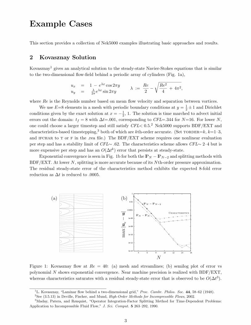
2 Kovasznay Solution

Kovasznay1 gives an analytical solution to the steady-state Navier-Stokes equations that is similar

to the two-dimensional flow-field behind a periodic array of cylinders (Fig. 1a),

ux = 1 − eλx cos 2πy

uy = λ2πe

λx sin 2πyλ :=

Re

2−

√

Re2

4+ 4π2,

where Re is the Reynolds number based on mean flow velocity and separation between vortices.

We use E=8 elements in a mesh with periodic boundary conditions at y = 1

2± 1 and Dirichlet

conditions given by the exact solution at x = −1

2, 1. The solution is time marched to advect initial

errors out the domain: tf = 8 with ∆t=.001, corresponding to CFL=.344 for N=16. For lower N ,

one could choose a larger timestep and still satisfy CFL< 0.5.2 Nek5000 supports BDF/EXT and

characteristics-based timestepping,3 both of which are kth-order accurate. (Set torder=k, k=1–3,

and ifchar to t or f in the .rea file.) The BDF/EXT scheme requires one nonlinear evaluation

per step and has a stability limit of CFL∼ .62. The characteristics scheme allows CFL∼ 2–4 but is

more expensive per step and has an O(∆tk) error that persists at steady-state.

Exponential convergence is seen in Fig. 1b for both the lPN − lPN−2 and splitting methods with

BDF/EXT. At lower N , splitting is more accurate because of its Nth-order pressure approximation.

The residual steady-state error of the characteristics method exhibits the expected 8-fold error

reduction as ∆t is reduced to .0005.

1e-14

1e-12

1e-10

1e-08

1e-06

0.0001

0.01

1

4 6 8 10 12 14 16

max

|ue−u|

N

lPN − lPN

lPN − lPN−2

Characteristics

(b)(a)

Figure 1: Kovasznay flow at Re = 40: (a) mesh and streamlines; (b) semilog plot of error vs

polynomial N shows exponential convergence. Near machine precision is realized with BDF/EXT,

whereas characteristics saturates with a residual steady-state error that is observed to be O(∆t3).

1L. Kovasznay, “Laminar flow behind a two-dimensional grid,” Proc. Cambr. Philos. Soc. 44, 58–62 (1948).2See (3.5.13) in Deville, Fischer, and Mund, High-Order Methods for Incompressible Flows, 2002.3Maday, Patera, and Rønquist, “Operator Integration-Factor Splitting Method for Time-Dependent Problems:

Application to Incompressible Fluid Flow,” J. Sci. Comput. 5 263–292, 1990.

3

3 Rayleigh-Benard Convection

Chandrasekhar4 has carefully studied linear stability of Rayleigh-Benard convection using the

Boussinesq approximation, given in terms of the Rayleigh (Ra) and Prandtl (Pr) numbers as

∂u

∂t+ u · ∇u = −∇p+ Pr∇2u−RaPrT,

∂T

∂t+ u · ∇T = ∇2T,

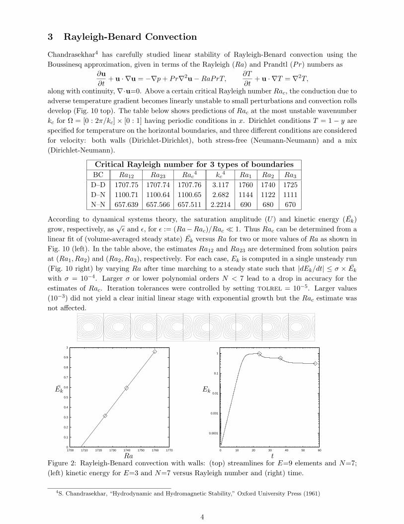
along with continuity, ∇·u=0. Above a certain critical Rayleigh number Rac, the conduction due to

adverse temperature gradient becomes linearly unstable to small perturbations and convection rolls

develop (Fig. 10 top). The table below shows predictions of Rac at the most unstable wavenumber

kc for Ω = [0 : 2π/kc] × [0 : 1] having periodic conditions in x. Dirichlet conditions T = 1 − y are

specified for temperature on the horizontal boundaries, and three different conditions are considered

for velocity: both walls (Dirichlet-Dirichlet), both stress-free (Neumann-Neumann) and a mix

(Dirichlet-Neumann).

Critical Rayleigh number for 3 types of boundaries

BC Ra12 Ra23 Rac4 kc

4 Ra1 Ra2 Ra3

D–D 1707.75 1707.74 1707.76 3.117 1760 1740 1725

D–N 1100.71 1100.64 1100.65 2.682 1144 1122 1111

N–N 657.639 657.566 657.511 2.2214 690 680 670

According to dynamical systems theory, the saturation amplitude (U) and kinetic energy (Ek)

grow, respectively, as√ǫ and ǫ, for ǫ := (Ra−Rac)/Rac ≪ 1. Thus Rac can be determined from a

linear fit of (volume-averaged steady state) Ek versus Ra for two or more values of Ra as shown in

Fig. 10 (left). In the table above, the estimates Ra12 and Ra23 are determined from solution pairs

at (Ra1, Ra2) and (Ra2, Ra3), respectively. For each case, Ek is computed in a single unsteady run

(Fig. 10 right) by varying Ra after time marching to a steady state such that |dEk/dt| ≤ σ × Ek

with σ = 10−4. Larger σ or lower polynomial orders N < 7 lead to a drop in accuracy for the

estimates of Rac. Iteration tolerances were controlled by setting tolrel = 10−5. Larger values

(10−3) did not yield a clear initial linear stage with exponential growth but the Rac estimate was

not affected.

0

0.1

0.2

0.3

0.4

0.5

0.6

0.7

0.8

0.9

1

1700 1710 1720 1730 1740 1750 1760 1770

Ek

Ra

0.0001

0.001

0.01

0.1

1

0 10 20 30 40 50 60

Ek

tFigure 2: Rayleigh-Benard convection with walls: (top) streamlines for E=9 elements and N=7;

(left) kinetic energy for E=3 and N=7 versus Rayleigh number and (right) time.

4S. Chandrasekhar, “Hydrodynamic and Hydromagnetic Stability,” Oxford University Press (1961)

4

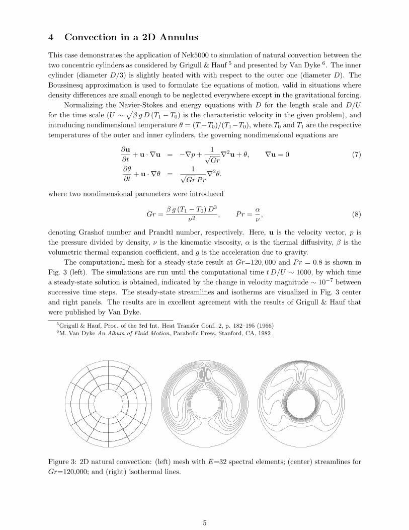
4 Convection in a 2D Annulus

This case demonstrates the application of Nek5000 to simulation of natural convection between the

two concentric cylinders as considered by Grigull & Hauf 5 and presented by Van Dyke 6. The inner

cylinder (diameter D/3) is slightly heated with with respect to the outer one (diameter D). The

Boussinesq approximation is used to formulate the equations of motion, valid in situations where

density differences are small enough to be neglected everywhere except in the gravitational forcing.

Normalizing the Navier-Stokes and energy equations with D for the length scale and D/U

for the time scale (U ∼√

β g D (T1 − T0) is the characteristic velocity in the given problem), and

introducing nondimensional temperature θ = (T−T0)/(T1−T0), where T0 and T1 are the respectivetemperatures of the outer and inner cylinders, the governing nondimensional equations are

∂u

∂t+ u · ∇u = −∇p+ 1√

Gr∇2u+ θ, ∇u = 0 (7)

∂θ

∂t+ u · ∇θ =

1√Gr Pr

∇2θ.

where two nondimensional parameters were introduced

Gr =β g (T1 − T0)D

3

ν2, P r =

α

ν, (8)

denoting Grashof number and Prandtl number, respectively. Here, u is the velocity vector, p is

the pressure divided by density, ν is the kinematic viscosity, α is the thermal diffusivity, β is the

volumetric thermal expansion coefficient, and g is the acceleration due to gravity.

The computational mesh for a steady-state result at Gr=120, 000 and Pr = 0.8 is shown in

Fig. 3 (left). The simulations are run until the computational time tD/U ∼ 1000, by which time

a steady-state solution is obtained, indicated by the change in velocity magnitude ∼ 10−7 between

successive time steps. The steady-state streamlines and isotherms are visualized in Fig. 3 center

and right panels. The results are in excellent agreement with the results of Grigull & Hauf that

were published by Van Dyke.

5Grigull & Hauf, Proc. of the 3rd Int. Heat Transfer Conf. 2, p. 182–195 (1966)6M. Van Dyke An Album of Fluid Motion, Parabolic Press, Stanford, CA, 1982

Figure 3: 2D natural convection: (left) mesh with E=32 spectral elements; (center) streamlines for

Gr=120,000; and (right) isothermal lines.

5

5 Navier-Stokes Eigenfunctions

Walsh7 derived a family of exact eigenfunctions for the Stokes and Navier-Stokes equations based

on a generalization of Taylor-Green vortices in the periodic domain Ω = [0, 2π]2. For all integer

pairs (m,n) satisfying λ = −(m2+n2), families of eigenfunctions can be formed by defining stream-

functions that are linear combinations of the functions

cos(mx) cos(ny), sin(mx) cos(ny), cos(mx) sin(ny), sin(mx) sin(ny).

Taking as an initial condition the eigenfunction u′ := (−ψy, ψx), a solution to the Navier-Stokes

equations is u = eνλtu′(x). (Note that pressure precisely balances the 2m and 2n wavenumbers

arising from the quadratic terms, as it must.) Figure 4 shows the vorticity for a case proposed by

Walsh, with ψ = (1/4) cos(3x) sin(4y) − (1/5) cos(5y) − (1/5) sin(5x). The solution is stable only

for modest Reynolds numbers. Interesting long-time solutions can be realized, however, by adding

a relatively high-speed mean flow u0, in which case the solution is u(x, t) = u0 + eνλtu′[x − u0t],

where the brackets imply that the argument is modulo 2π in x and y. By varying u0, one can

advect the solution a significant number of characteristic lengths before the eigensolution decays.

The right two panels in Fig. 4 show the spatial and temporal errors for the solution on the

left with ν = .05 and u0 = (16, 5), for which a feature of characteristic length l=2π/5 is propagated

≈ 25l by final time t=2. The center panel shows that characteristics scheme yields expected kth-

order accuracy when torder=k, k=2 or 3. The right panel shows that exponential convergence

vs. N for both the lPN − lPN−2 and lPN − lPN methods, with the latter having lower error. As N

is increased, the error saturates to the temporal truncation error. For the characteristics scheme,

the error for ∆t=.0001 is 5.8×10−8, while for extrapolation it is 1.4×10−6. In contrast to the

steady-state Kovasznay case, the characteristics scheme is more accurate than extrapolation.

Also shown in the right panel is the error for the lPN − lPN−2/characteristics combination

when using a mesh comprising E=E1 ×E1 elements, with E1=4 and 8. For the E1=4 case, a final

error of < .01 is realized with N=7, corresponding to 5.6 points/wavelength. For E1=8, a final

error of .0023 is attained with N=5, corresponding to 8 points per wavelength.

1e-09

1e-08

1e-07

1e-06

1e-05

0.0001

0.0001 0.001

max

|ue(x,2)−u(x,2)|

∆t

Torder=2

Torder=3

1e-08

1e-07

1e-06

1e-05

0.0001

0.001

0.01

0.1

1

2 4 6 8 10 12 14 16

’err.b2’ u 2:6’err.c2’ u 2:6’err.b4’ u 2:6’err.c4’ u 2:6’err.E4’ u 2:6’err.E8’ u 2:6

max

|ue(x,2)−u(x,2)|

N

Extr.

Char.

E1=4

E1=8

E1=16

Figure 4: Eddy solution results: (left) vorticity at t=2 for N=15, (center) error vs ∆t for

lPN − lPN−2 with N=15 and ifchar=t, and (right) error vs polynomial order N for lPN − lPN−2

and lPN − lPN with ∆t=.0001 and ifchar=f/t (i.e., extrapolation or characteristics).

7O. Walsh, “Eddy solutions of the Navier-Stokes equations,” The NSE II-Theory and Numerical Methods, J.G.

Heywood, K. Masuda, R. Rautmann, and V.A. Solonikkov, eds., Springer, pp. 306–309 (1992)

6

6 Inviscid Vortex Propagation

Propagation of an inviscid vortex has been used as a test problem in earlier studies of finite volume

methods.8,9 The domain is two dimensional with uniform inflow u = 1 at x = −0.5, outflow

conditions at x = 3.5, and symmetry boundary condtitions at y = ±0.5. The initial condition is a

vortex in a mean flow, (u, v) = (1 − yuθ, xuθ), where uθ = 5r, 0 ≤ r < 0.2; 2 − 5r, 0.2 ≤ r < 0.4;

0, 0.4 ≤ r. Two spectral element meshes are considered. The first is an 8×2 array of square

elements with N=10, the second is 16×4 with N=5, for a total resolution of 81 × 21. We use

the dealiased lPN − lPN formulation (lx2=lx1) with viscosity ν = 10−50 and integrate to t=4.0,

at which point the vortex has left the domain. We consider 3rd-order characteristics timestepping

with ∆t=.0125 and BDF3/EXT3 with ∆t=.005. For each of the four cases, we consider filtered

and non-filtered results with filter parameters p103=.05 for ∆t=.0125 and p103=.02 for ∆t=.005,

giving essentially the same filter strength per unit time. For N=5 we filter the Nth mode only,

whereas for for N=10 we filter both the N and N -1 modes, with the latter damped by p103/4.

Figure 5a shows the vortex structures at t=0,1,2,3 side by side for the filtered (p101=.02)

case with N=5. The vortex is not Rayleigh stable and thus destabilized by any perturbation.

High-resolution runs indicate that t=3 is about the limit of stability and one can see the elongation

of the vortex at this time in the right-most image. Figures 5b and c show the vortex energy, which

should be constant until the vortex leaves the domain. For all of the simulations, the vortex retains

> 98.8% of it’s initial energy to t=3. The most diffusive cases are the filtered simulations with

N=5, which show a 1.1–1.2% energy loss. The N=10 cases show ∼0.5% energy loss at t=3.

(a)

(b)

0

0.2

0.4

0.6

0.8

1

1.2

0 0.5 1 1.5 2 2.5 3 3.5 4 4.5

’v.n05_f00’ u 2:3’v.n05_f02’ u 2:3’v.n05_c00’ u 2:3’v.n05_c05’ u 2:3

0.96

0.98

1

1.02

1.04

0 0.5 1 1.5 2 2.5 3 3.5 4 4.5

’v.n05_f00’ u 2:3’v.n05_f02’ u 2:3’v.n05_c00’ u 2:3’v.n05_c05’ u 2:3

(c)

0

0.1

0.2

0.3

0.4

0.5

0.6

0.7

0.8

0.9

1

1.1

0 0.5 1 1.5 2 2.5 3 3.5 4 4.5

’v.n10_f00’ u 2:3’v.n10_f02’ u 2:3’v.n10_c00’ u 2:3’v.n10_c05’ u 2:3

0.96

0.98

1

1.02

1.04

0 0.5 1 1.5 2 2.5 3 3.5 4 4.5

’v.n10_f00’ u 2:3’v.n10_f02’ u 2:3’v.n10_c00’ u 2:3’v.n10_c05’ u 2:3

Figure 5: Propagation of an inviscid vortex: (a) contours of vorticity at t=0, 1, 2, and 3 for filtered

simulation with N=5 and BDF3/EXT3, (b) energy vs time for N=5, and (c) N=10.

8P.J. O’Rourke and M.S. Sahota, “A Variable Explicit/Implicit Numerical Method for Calculating Advection on

Unstructured Meshes,” J. Comp. Phys. 143 312–345 (1998)9M.S. Sahota, P.J. O’Rourke, M.C. Cline, “Assessment of Vorticity and Angular Momentum Errors in CHAD for

the Gresho Problem,” Tech. Rep. LA-UR-00-2217, Theor. Fluid Dyn., Los Alamos National Laboratory, May 2000.

7

7 Stability of Free-Surface Channel Flow

As a check of the free-surface ALE formulation in Nek5000, we compare the growth rate for the

most unstable mode for a falling film with results from linear theory.10 For perturbation size ǫ, one

can expect O(ǫ) agreement in growth rate between linear and nonlinear models.

The nominal computational domain was taken as Ω = [0, 2π]× [−1, 0], tesselated with a 6×10

array of spectral elements. A uniform element distribution was used in the streamwise direction

while a stretched distribution was used in the wall-normal direction. Near the wall, an element

thickness of ∆y=.005 was used to resolve the boundary layer of the unstable eigenmodes. The

polynomial order within each element was N = 13 and BDF3/EXT3 timestepping was used with

∆t=.00125. The initial conditions corresponded to the base flow plus ǫ := 10−5 times the most

unstable eigenmode for these particular flow conditions. The domain was stretched using an affine

mapping in y to accomodate the O(ǫ) surface displacement. The eigenmodes, which are defined

only on y = [-1, 0], were mapped onto the nominal domain then displaced along with the mesh.

The base flow was defined as U(y) = 1 − y2 over the deformed mesh. The Reynolds number was

Re=30000, Weber numberWe=0.011269332539972, and gravitational Prandtl number Pg=.00011.

The applied body force was f = (2Re−1,−(RePg)−2) and the surface tension was σ =We.

Mean growth rates were computed by monitoring the L2-norm of the wall-normal velocity v

and defining γ(t) := t−1 ln(||v(x, t)||2/||v(x, 0)||2). The error is defined as e(t) := (γ(t) − γ∗)/γ∗

where γ∗=0.007984943826436 is computed using linear theory. Aside from some initial transients,

the error over t = [0,200] was less than .0005.

Initial tests for this problem revealed blow-up at fairly late times (t ∼ 160). The locality and

high wavenumber content in the error indicates that the blow-up is due to lack of de-aliasing in

certain nonlinear terms associated with the ALE formulation. (The convective terms were dealiased;

p99=3.) As illustrated in Fig. 6, such high wavenumber errors are readily addressed with low pass

filtering, here implemented with p103=.05 and p101=2. We note that the error in the predicted

growth rate does increase at t > 1000 for reasons unknown at this point, but which might be

attributable to true nonlinear effects (i.e., departure from linearity).

-0.0005

0

0.0005

0.001

0.0015

0.002

0 20 40 60 80 100 120 140 160 180 200

’f.a’ u 2:9’t.a’ u 2:9

(γ(t)−γ∗)/γ∗

time t

unfiltered

filtered

Figure 6: Eigenmodes for free-surface film flow: (left, top) contours of vertical velocity v for

unfiltered and (left, bottom) filtered solution at time t = 179.6; (right) error in growth rate vs. t.

10Instabilities in free-surface Hartmann flow at low magnetic Prandtl numbers. Giannakis, D., Rosner, R., &

Fischer, P.F. 2009, J. Fluid Mech., 636, 217-277

8

8 Stratified 2D Flows

This note illustrates some basic phenomena of stratified flows computed with Nek5000 using a

Boussinesq approximation. We consider a two-dimensional flow with free-stream velocity U past

a cylinder of diameter D and examine blocking, the Brunt-Vasailla frequency, and the wave-like

nature of stratified flow. Our discussion closely follows the introductory material given by Tritton.11

We assume that the density of the fluid is given by ρ = ρ0 + ρ′(x, t), where the background

density ρ0 ≫ ρ′ is constant. To first order, the perturbation ρ′ only acts through the gravitational

forcing in the momentum equations, given in dimensional form by

ρ0

(

∂u

∂t+ u · ∇u

)

= −∇p+ ρ0ν∇2u− g(

ρ0 + ρ′)

y. (9)

The constant −gρ0y can be absorbed into the pressure (as can any other potential field), so the

dynamical influence of the stratification is driven only by the perturbation density ρ′. In addition

to (9), we have the standard incompressibility constraint

∇ · u = 0, (10)

and the transport equation

∂ρ′

∂t+ u · ∇ρ′ = κ∇2ρ′, (11)

which reflects the fact that the density perturbation is tied to a scalar quantity, such as salinity or

temperature, that satisfies a convection-diffusion equation. (Note that Nek5000 readily handles a

variable ρ0 as well. The current studies, however, follow the formulation given by (9)–(11).)

We assume a linear profile for the initial condition of (11). That is,

ρ′y,0 :=∂ρ′

∂y

∣

∣

∣

∣

t=0

= constant.

Under these circumstances, there is an intrinsic timescale associated the stratification, which is

usually expressed by its inverse, namely, the Brunt-Vasailla frequency:

NBV :=

(

g

ρ0ρ′y,0

)1

2

. (12)

We return to this in the discussion below but introduce it here, prior to nondimensionalization, to

stress that it is independent of any timescale associated with the external flow.

Before proceeding with the examples, we rescale the governing system of equations by the

length scale D and convective timescale D/U to arrive at the nondimensional system

∂u

∂t+ u · ∇u = −∇p+ 1

Re∇2u− 1

Fr2(ρ′ − y)y (13)

∇ · u = 0 (14)

∂ρ′

∂t+ u · ∇ρ′ =

1

PrRe∇2ρ′. (15)

Here, we have slightly abused the notation by using the same symbols for the dimensional and

nondimensional variables; there will be no confusion, however, given the context in which each

11D.J. Tritton, Physical Fluid Dynamics, Oxford (1988).

9

is used. In addition to rescaling, we divided (9) and normalized the pressure by ρ0, and have

introduced three nondimensional parameters,

Re =UD

ν, Pr =

κ

ν, Fr−2 =

gD2

ρ0U2

∣

∣ρ′y,0∣

∣ , (16)

which are, respectively, the Reynolds number, the Prandtl (or Schmidt) number, and the Froude

number. Note that the it is common to replace the Froude number by the Richardson number,

Ri := Fr−2. Finally, we have introduced an additional potential,

− 1

Fr2yy, (17)

to remove the hydrostatic mode (associated with ρ′) from the pressure.

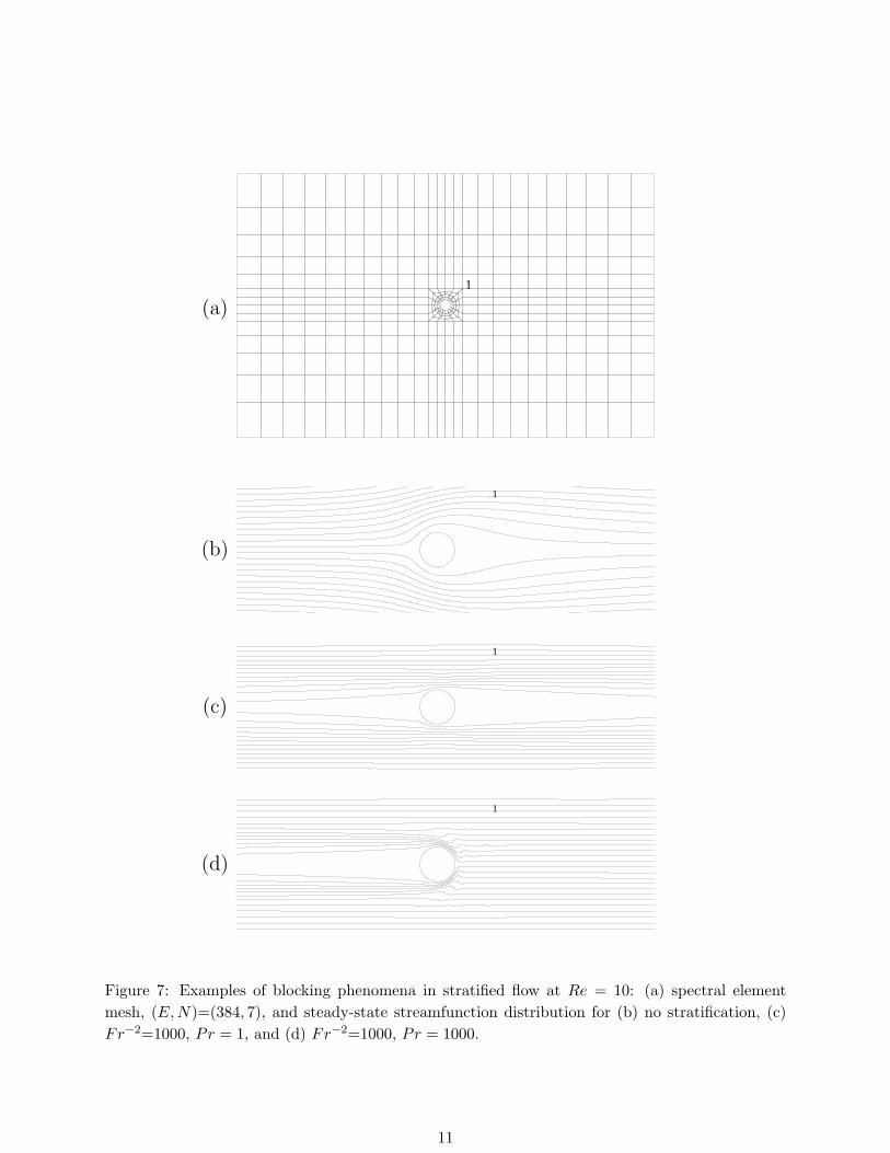
We have computed steady-state flow past a cylinder at Re = 10 using the two-dimensional

mesh shown in Fig. 7(a). The mesh comprises E = 346 elements of order N = 7. A uniform inflow

of speed U = 1 is specified at the left boundary and symmetry conditions are specified on the top

and bottom boundaries. The Neumann (natural) condition for the Stokes problem,

∂ui∂n

+ p = 0, i = 1, 2,

is applied on the right boundary, which effectively corresponds to having p = 0 at the outflow. It

is for this reason that we use (17) to remove the hydrostatic contribution to the pressure.

The solutions are time-marched to steady state. The initial condition for the unstratified case

of Fig. 7(a) was u = (1, 0, 0). The converged steady-state velocity field of (a) was used as the

initial condition for the stratified cases (b) and (c). the initial density profiles were ρ′ = −y. (Thecylinder is centered at (0, 0).)

8.1 Steady State Results

Figures 7(b)–(d) show steady-state streamline patterns under different stratification conditions.

Case (b) is standard Navier-Stokes flow without stratification. It exhibits a classic wake structure

with flow separation at roughly 29 degrees from the horizontal axis and a small recirculation zone

of length ≈ D/4 aft of the cylinder.

The streamline patterns in Fig. 7(c) and (d) are in marked contrast to those in (b). In Fig.

7(c), we see that there are wakes both in front and behind the cylinder, while in (d) there is a wake

only in front of the cylinder. In (c) and (d), the Froude number is Fr = 10001/2, which corresponds

to significant stratification. This results in a phenomenon known as blocking, which occurs when

the dynamic head of the fluid is insufficient to overcome the potential energy barrier associated

with climbing above (or descending below) the cylinder. Fluid particles are essentially trapped at

a given height. As explained in Tritton, the length of the forward wake is determined by viscous

effects, and scales as O(Re/Fr2), provided the domain is sufficiently large.

While the flow upstream of the cylinder in Figs. 7(c) and (d) is similar in structure, the

downstream behavior is decidely different. The flow conditions in (c) and (d) are identical, save

that Pr = 1 in (c) and Pr = 1000 in (d). The change in the flow behavior can be explained as

follows. Through density diffusion, a fluid parcel that flows close to the cylinder in case (c) takes

on the local density by the time it reaches the cylinder apex. As it passes the cylinder, it has a

tendency to remain at its new height and thus only slowly returns to its original height, resulting

in an extended wake. For large Pr, however, the density diffusion is small. A particle passing the

cylinder thus retains its original density and quickly returns to its original height after passing the

cylinder. This results in the streamline pattern of Fig. 7(d). (Note that the Schmidt number for

salt water is Sc ≈ 700, so Pr = 1000 is not far from being physically realizable.)

10

1

1

1

1

(a)

(b)

(c)

(d)

Figure 7: Examples of blocking phenomena in stratified flow at Re = 10: (a) spectral element

mesh, (E,N)=(384, 7), and steady-state streamfunction distribution for (b) no stratification, (c)

Fr−2=1000, Pr = 1, and (d) Fr−2=1000, Pr = 1000.

11

1

-0.6

-0.4

-0.2

0

0.2

0.4

0.6

0.8

0 1 2 3 4 5 6 7 8

-0.06

-0.04

-0.02

0

0.02

0.04

0.06

0.08

5 5.5 6 6.5 7

(a)

(b)

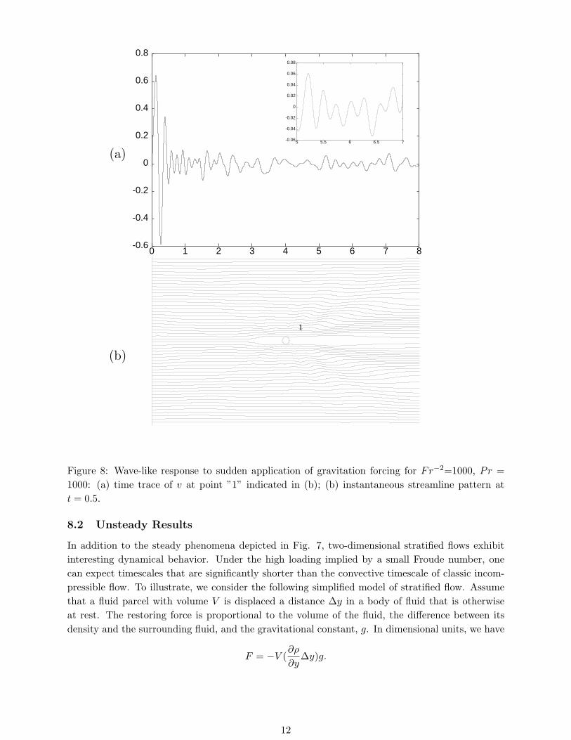
Figure 8: Wave-like response to sudden application of gravitation forcing for Fr−2=1000, Pr =

1000: (a) time trace of v at point ”1” indicated in (b); (b) instantaneous streamline pattern at

t = 0.5.

8.2 Unsteady Results

In addition to the steady phenomena depicted in Fig. 7, two-dimensional stratified flows exhibit

interesting dynamical behavior. Under the high loading implied by a small Froude number, one

can expect timescales that are significantly shorter than the convective timescale of classic incom-

pressible flow. To illustrate, we consider the following simplified model of stratified flow. Assume

that a fluid parcel with volume V is displaced a distance ∆y in a body of fluid that is otherwise

at rest. The restoring force is proportional to the volume of the fluid, the difference between its

density and the surrounding fluid, and the gravitational constant, g. In dimensional units, we have

F = −V (∂ρ

∂y∆y)g.

12

This force accelerates the parcel in a direction opposite to ∆y, resulting in the equation of motion

d2∆y

dt2+

(

g

ρ

∂ρ

∂y

)

∆y = 0,

which obviously leads to simple harmonic motion with frequency

NBV :=

√

g

ρ

∂ρ

∂y.

Because U=1 and D=1 in the current nondimensionalization, we have from (16) NBV = Ri1

2 =

Fr−1, with corresponding period τBV = 2πFr.

Figure 8(a) shows the history of the vertical velocity component at the point indicated by the

“1” in Fig. 8(b). The initial conditions for u and ρ′ are taken to be the steady-state flow conditions

of Fig. 7(b), with Pr=1000. When the forcing is turned on, the density distribution is far from

equilibrium and oscillations ensue. The oscillations in the inset in Fig. 8(a) correspond to a period

of τ ≈ 0.257, in close agreement with τBV = .199. That τ > τBV can be understood by the fact

that, because of incompressibility and the boundary conditions, the vertical displacement of any

given fluid parcel must be associated with the horizontal displacement of some other parcels that

add mass to the displaced system but do not add potential energy. As a consequence, the frequency

will be lowered.

Tritton carries the unsteady analysis further and points out that disturbances in stably strat-

ified flows can propagate as waves. Wave patterns are clearly evident in Fig. 8(b), which shows

the instantaneous streamlines at time t = 0.5 for the flow associated with Fig. 8(a). Note that

this convective time corresponds to the time it takes a particle in the free stream to move half a

diameter. However, the wake structures and multiple waves can be seen to extend several diameters

away from from the cylinder at this early time. We note that the loading is applied instantaneously

throughout the domain, and that the nonequilibrium displacement of ρ′ at t = 0 may already extend

several diameters in the initial conditions.) Nonetheless, it is clear from Fig. 8(b) and other similar

early-time images that information is propagating on a timescale that is much shorter than the

convective timescale.

Tritton also derives a dispersion relationship for the wave phenomenon that gives the frequency

as a function of the vectorial wave number

ω = NBV sin θ,

where θ is the angle of the wave vector with respect to the vertical axis. From the preceding

estimates of τ , we can estimate the angle of the wave vector to be ≈ 50.6 degrees, which is in

reasonable agreement with the pattern observed near history point “1” in Fig. 8(b).

8.3 Implications for Simulation

We close with a few numerical considerations encountered in these simulations.

First, because the bouyancy force is treated explicitly in Nek5000 and because it is associated

with a fast timescale (for small Fr), the timestep size will generally be much less than the usual

Courant-limited timestep.

Second, it is important to respect p = 0 at the outflow boundary, as much as possible. Also,

it is important to start the simulation close to equilibrium. Otherwise, the wave motions can suck

fluid in through the outflow boundary, which is usually disastrous.

13

Third, the wavelike nature of stratified flow implies a potential need for radiation boundary

conditions, if significant wave energy is to leave the domain through an artificial domain boundary.

Fourth, we note that NBV is based upon the vertical density gradient. In the case of a sharp

interface, with densities ρ′1and ρ′

2on either side, it should be redefined in terms of the density

jump ρ′2− ρ′

1.

Fifth, turbulence, if present, will generally yield an order-unity (effective) Prandtl/Schmidt

number.

14

X

Y

Z

X Y

Z

X Y

Z

-0.02

0

0.02

0.04

0.06

0.08

0.1

0 0.5 1 1.5 2

’prof.1854’ u 3:6’prof.1492’ u 3:6

0

Re=1854

Re=1492

z

w

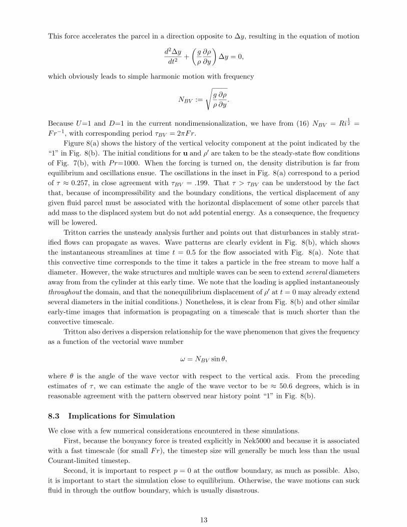
Figure 9: Vortex breakdown results: (left) streamlines for Re=1854, (center) in-plane streamlines

for Re=1854, (right) vertical velocity distributions along the centerline.

9 Vortex Breakdown

Escudier12 studied vortex breakdown in a container with a rotating lid. The domain consists of a

cylindrical container of radius R and height H = 2R. The top lid rotates at a constant angular

velocity Ω, and the Reynolds number is Re = Ω2R/ν. Following the standard approach, we take

Ω = R = ρ = 1 and set ν = Re−1.

The mesh in Fig. 9 is constructed from a 2D base swept through z with element boundaries

at z=0, 0.06, 0.4, 0.8, 1.2, 1.6, 1.95, and 2. The mesh is concentrated near the cannister walls and

near the upper and lower lids. The singularity at r=R, z=2 is handled by shearing the side walls

in the top layer of elements using a 5th-order monomial. The initial and boundary condition for

z > 1.95 are thus (u, v) = (−y, x) ∗ α(z), with α = (z − 2)5/∆5z and ∆z = .05. The simulations are

time-marched to steady state at varying spatial resolutions (N=7, 9, and 11). Simulation times of

tf ≈ 1000 are required to form a single bubble in the Re = 1492 case.

Depending on the aspect ratio and Reynolds number, one can find various steady and unsteady

vortex breakdown regimes with one or more “bubbles” (reversal regions) on the axis. For H/R=2,

Escudier documented steady-state flows with with a single bubble at Re=1492 and two bubbles

at Re=1854. The streamline plots in Fig. 9 show the bubble structures for Re=1854. Bubble

locations can be inferred from zero-crossings of axial velocity w versus z at (x, y) = (0, 0), shown in

the right panel. These locations are tabulated below, along with experimental results of Escudier

and numerical results of Sotiropoulos and Ventikos.13

Locations of Vertical Velocity Reversals

Re=1492 Re=1854

z1 z2 z1 z2 z3 z4

N=7 .689 .836 .427 .793 .960 1.131

N=9 .671 .831 .420 .776 .954 1.118

N=11 .671 .831 .420 .775 .955 1.117

Escudier .68 .80 .42 .74 1.04(?) 1.18(?)

Sot. & Ven .646 .774 .42 .772 .928 1.09

12M.P. Escudier, “Observations of the flow produced in a cylindrical container by a rotating endwall,” Exp. Fluids

2 189–196 (1984).13F. Sotiropoulos & Y. Ventikos, “Transition from bubble-type vortex breakdown to columnar vortex in a confined

swirling flow,” Int. J. Heat and Fluid Flow 19 446–458 (1998).

15

10 Axisymmetric Rayleigh-Benard Convection

14

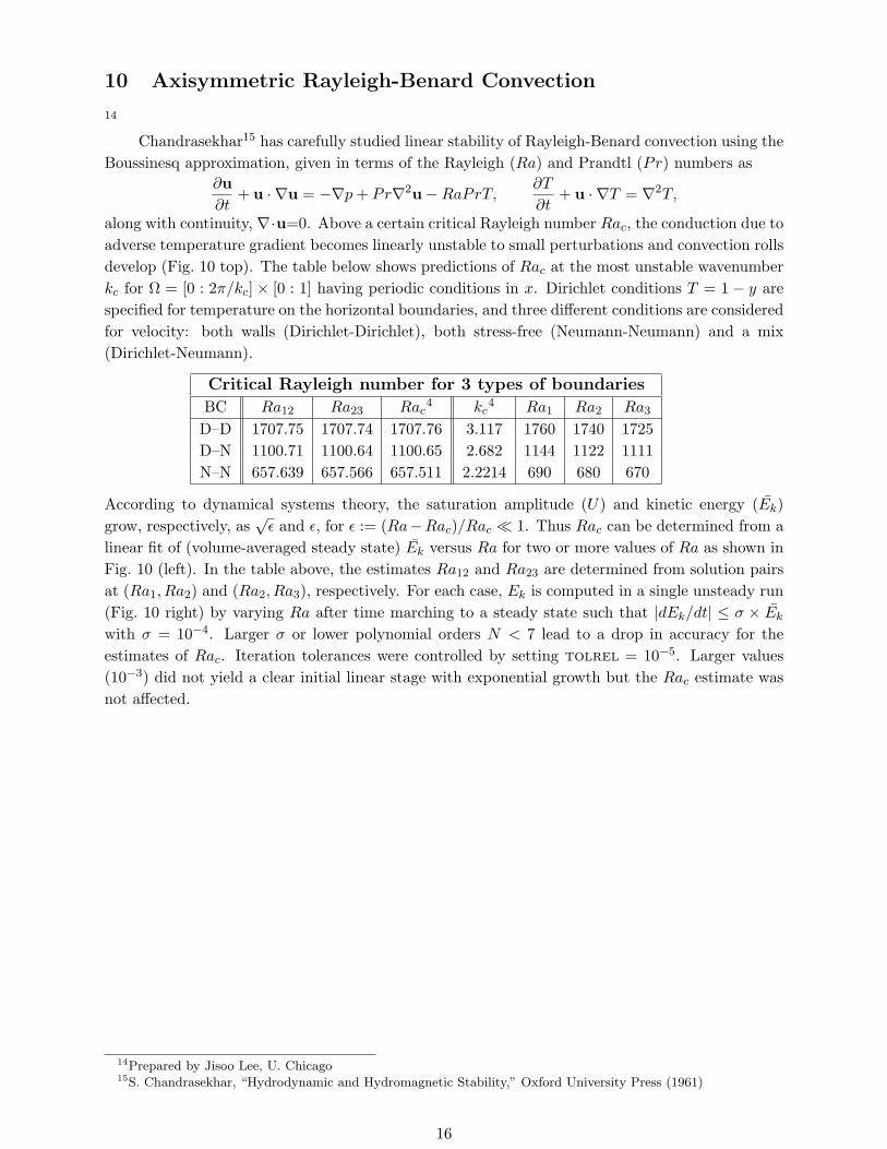
Chandrasekhar15 has carefully studied linear stability of Rayleigh-Benard convection using the

Boussinesq approximation, given in terms of the Rayleigh (Ra) and Prandtl (Pr) numbers as

∂u

∂t+ u · ∇u = −∇p+ Pr∇2u−RaPrT,

∂T

∂t+ u · ∇T = ∇2T,

along with continuity, ∇·u=0. Above a certain critical Rayleigh number Rac, the conduction due to

adverse temperature gradient becomes linearly unstable to small perturbations and convection rolls

develop (Fig. 10 top). The table below shows predictions of Rac at the most unstable wavenumber

kc for Ω = [0 : 2π/kc] × [0 : 1] having periodic conditions in x. Dirichlet conditions T = 1 − y are

specified for temperature on the horizontal boundaries, and three different conditions are considered

for velocity: both walls (Dirichlet-Dirichlet), both stress-free (Neumann-Neumann) and a mix

(Dirichlet-Neumann).

Critical Rayleigh number for 3 types of boundaries

BC Ra12 Ra23 Rac4 kc

4 Ra1 Ra2 Ra3

D–D 1707.75 1707.74 1707.76 3.117 1760 1740 1725

D–N 1100.71 1100.64 1100.65 2.682 1144 1122 1111

N–N 657.639 657.566 657.511 2.2214 690 680 670

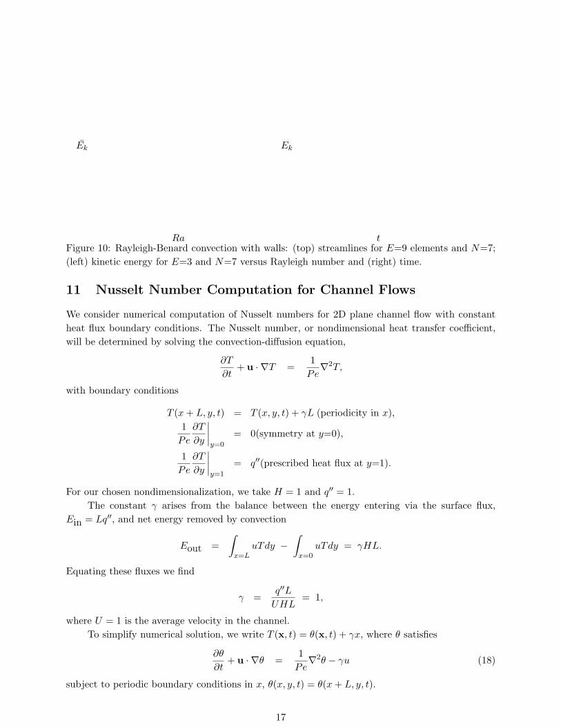
According to dynamical systems theory, the saturation amplitude (U) and kinetic energy (Ek)

grow, respectively, as√ǫ and ǫ, for ǫ := (Ra−Rac)/Rac ≪ 1. Thus Rac can be determined from a

linear fit of (volume-averaged steady state) Ek versus Ra for two or more values of Ra as shown in

Fig. 10 (left). In the table above, the estimates Ra12 and Ra23 are determined from solution pairs

at (Ra1, Ra2) and (Ra2, Ra3), respectively. For each case, Ek is computed in a single unsteady run

(Fig. 10 right) by varying Ra after time marching to a steady state such that |dEk/dt| ≤ σ × Ek

with σ = 10−4. Larger σ or lower polynomial orders N < 7 lead to a drop in accuracy for the

estimates of Rac. Iteration tolerances were controlled by setting tolrel = 10−5. Larger values

(10−3) did not yield a clear initial linear stage with exponential growth but the Rac estimate was

not affected.

14Prepared by Jisoo Lee, U. Chicago15S. Chandrasekhar, “Hydrodynamic and Hydromagnetic Stability,” Oxford University Press (1961)

16

Ek

Ra

Ek

tFigure 10: Rayleigh-Benard convection with walls: (top) streamlines for E=9 elements and N=7;

(left) kinetic energy for E=3 and N=7 versus Rayleigh number and (right) time.

11 Nusselt Number Computation for Channel Flows

We consider numerical computation of Nusselt numbers for 2D plane channel flow with constant

heat flux boundary conditions. The Nusselt number, or nondimensional heat transfer coefficient,

will be determined by solving the convection-diffusion equation,

∂T

∂t+ u · ∇T =

1

Pe∇2T,

with boundary conditions

T (x+ L, y, t) = T (x, y, t) + γL (periodicity in x),

1

Pe

∂T

∂y

∣

∣

∣

∣

y=0

= 0(symmetry at y=0),

1

Pe

∂T

∂y

∣

∣

∣

∣

y=1

= q′′(prescribed heat flux at y=1).

For our chosen nondimensionalization, we take H = 1 and q′′ = 1.

The constant γ arises from the balance between the energy entering via the surface flux,

Ein = Lq′′, and net energy removed by convection

Eout =

∫

x=LuTdy −

∫

x=0

uTdy = γHL.

Equating these fluxes we find

γ =q′′L

UHL= 1,

where U = 1 is the average velocity in the channel.

To simplify numerical solution, we write T (x, t) = θ(x, t) + γx, where θ satisfies

∂θ

∂t+ u · ∇θ =

1

Pe∇2θ − γu (18)

subject to periodic boundary conditions in x, θ(x, y, t) = θ(x+ L, y, t).

17

The heat transfer coefficient, h, is defined by the relationship

q′′ = h(Tw − Tb) = h(θw − θb),

where θw is the temperature at the wall (y = 1) and θb is the bulk (mixing-cup) temperature

θb :=

∫

Ωu θ dV

∫

Ωu dV

,

with u the x-component of the convecting field u. In the general case, one must consider temporal

and/or spatial averages of θw and θb, but the above definitions suffice for the particular case

considered here. For a fluid with conductivity k, the Nusselt number is

Nu :=Hh

k=

Pe

θw − θb.

18

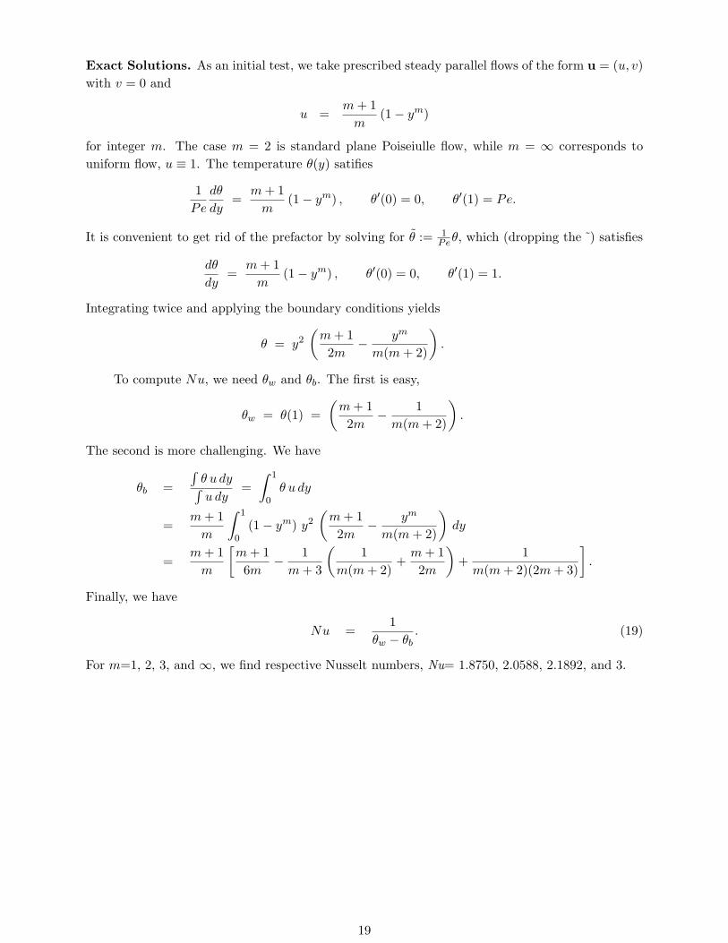
Exact Solutions. As an initial test, we take prescribed steady parallel flows of the form u = (u, v)

with v = 0 and

u =m+ 1

m(1− ym)

for integer m. The case m = 2 is standard plane Poiseiulle flow, while m = ∞ corresponds to

uniform flow, u ≡ 1. The temperature θ(y) satifies

1

Pe

dθ

dy=

m+ 1

m(1− ym) , θ′(0) = 0, θ′(1) = Pe.

It is convenient to get rid of the prefactor by solving for θ := 1

Peθ, which (dropping the ) satisfies

dθ

dy=

m+ 1

m(1− ym) , θ′(0) = 0, θ′(1) = 1.

Integrating twice and applying the boundary conditions yields

θ = y2(

m+ 1

2m− ym

m(m+ 2)

)

.

To compute Nu, we need θw and θb. The first is easy,

θw = θ(1) =

(

m+ 1

2m− 1

m(m+ 2)

)

.

The second is more challenging. We have

θb =

∫

θ u dy∫

u dy=

∫

1

0

θ u dy

=m+ 1

m

∫

1

0

(1− ym) y2(

m+ 1

2m− ym

m(m+ 2)

)

dy

=m+ 1

m

[

m+ 1

6m− 1

m+ 3

(

1

m(m+ 2)+m+ 1

2m

)

+1

m(m+ 2)(2m+ 3)

]

.

Finally, we have

Nu =1

θw − θb. (19)

For m=1, 2, 3, and ∞, we find respective Nusselt numbers, Nu= 1.8750, 2.0588, 2.1892, and 3.

19

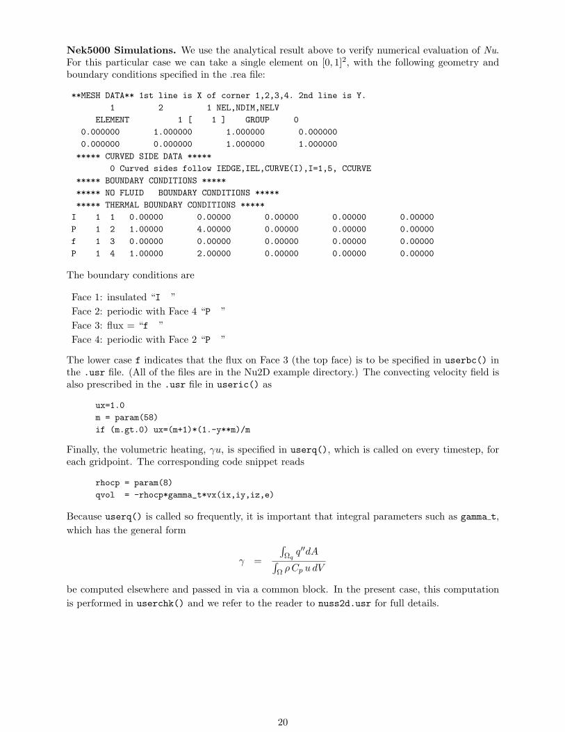
Nek5000 Simulations. We use the analytical result above to verify numerical evaluation of Nu.For this particular case we can take a single element on [0, 1]2, with the following geometry andboundary conditions specified in the .rea file:

**MESH DATA** 1st line is X of corner 1,2,3,4. 2nd line is Y.

1 2 1 NEL,NDIM,NELV

ELEMENT 1 [ 1 ] GROUP 0

0.000000 1.000000 1.000000 0.000000

0.000000 0.000000 1.000000 1.000000

***** CURVED SIDE DATA *****

0 Curved sides follow IEDGE,IEL,CURVE(I),I=1,5, CCURVE

***** BOUNDARY CONDITIONS *****

***** NO FLUID BOUNDARY CONDITIONS *****

***** THERMAL BOUNDARY CONDITIONS *****

I 1 1 0.00000 0.00000 0.00000 0.00000 0.00000

P 1 2 1.00000 4.00000 0.00000 0.00000 0.00000

f 1 3 0.00000 0.00000 0.00000 0.00000 0.00000

P 1 4 1.00000 2.00000 0.00000 0.00000 0.00000

The boundary conditions are

Face 1: insulated “I ”

Face 2: periodic with Face 4 “P ”

Face 3: flux = “f ”

Face 4: periodic with Face 2 “P ”

The lower case f indicates that the flux on Face 3 (the top face) is to be specified in userbc() inthe .usr file. (All of the files are in the Nu2D example directory.) The convecting velocity field isalso prescribed in the .usr file in useric() as

ux=1.0

m = param(58)

if (m.gt.0) ux=(m+1)*(1.-y**m)/m

Finally, the volumetric heating, γu, is specified in userq(), which is called on every timestep, foreach gridpoint. The corresponding code snippet reads

rhocp = param(8)

qvol = -rhocp*gamma_t*vx(ix,iy,iz,e)

Because userq() is called so frequently, it is important that integral parameters such as gamma t,

which has the general form

γ =

∫

Ωqq′′dA

∫

ΩρCp u dV

be computed elsewhere and passed in via a common block. In the present case, this computation

is performed in userchk() and we refer to the reader to nuss2d.usr for full details.

20

12 Unsteady Conduction with Robin Conditions

This example illustrates the use of Robin boundary conditions for the unsteady heat equation

∂u

∂t= ∇ · ν∇u, in Ω, αu+ β∇u · n = γ on ∂ΩR,

with either Dirichlet or Neumann conditions on the remainder of the domain boundary, ∂Ω\∂ΩR.

In this case, we consider the unit square, Ω = [0, 1]2, with ∂ΩR := [1, y] and homogeneous Neumann

conditions, ∇u · n = 0, elsewhere. Without loss of generality, we consider the case with γ = 0 and

initial condition u(t = 0, x, y)=1.

Under the stated conditions, a series solution exists of the form∑

k uk(t)φk(x) with

φk(x) = cos√

λkx,√

λk tan√

λk =α

β.

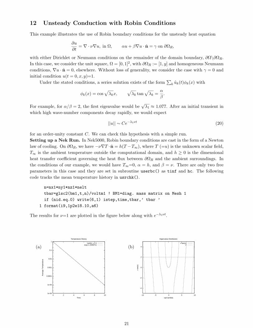
For example, for α/β = 2, the first eigenvalue would be√λ1 ≈ 1.077. After an initial transient in

which high wave-number components decay rapidly, we would expect

||u|| ∼ Ce−λ1νt (20)

for an order-unity constant C. We can check this hypothesis with a simple run.

Setting up a Nek Run. In Nek5000, Robin boundary conditions are cast in the form of a Newton

law of cooling. On ∂ΩR, we have −ν∇T · n = h(T −T∞), where T (=u) is the unknown scalar field,

T∞ is the ambient temperature outside the computational domain, and h ≥ 0 is the dimensional

heat transfer coefficient governing the heat flux between ∂ΩR and the ambient surroundings. In

the conditions of our example, we would have T∞=0, α = h, and β = ν. There are only two free

parameters in this case and they are set in subroutine userbc() as tinf and hc. The following

code tracks the mean temperature history in usrchk().

n=nx1*ny1*nz1*nelt

tbar=glsc2(bm1,t,n)/voltm1 ! BM1=diag. mass matrix on Mesh 1

if (nid.eq.0) write(6,1) istep,time,tbar,’ tbar ’

1 format(i9,1p2e18.10,a6)

The results for ν=1 are plotted in the figure below along with e−λ1νt.

(a)

1e-06

1e-05

0.0001

0.001

0.01

0.1

1

0 2 4 6 8 10

Ave

rage

Tem

pera

ture

Time

Temperature History

’nek5k’ u 2:3exp(-1.15993*x)

(b)

-4

-2

0

2

4

-10 -5 0 5 10

x ta

n(x)

sqrt lambda

Eigenvalue Distribution

x*tan(x)2

21