neighbour-sensing version 3 - david moore€¦ · our website offers for download a short video (it...

Neighbour-Sensing program v. 3.7 operating details as of 19/02/2017

© Audrius Meškauskas & David Moore 2017. All rights reserved.



Neighbour-Sensing User manual

Operating details for version 3.7 of the

Neighbour-Sensing program for creating life-like

three-dimensional simulations of growing fungal

mycelia and tissues

The program is distributed as .msi files, freeware to

download from our website at

www.davidmoore.org.uk\CyberWEB\Downloads

http://www.davidmoore.org.uk/CyberWEB/Downloads



INSTALLING THE PROGRAM

Installing only the Neighbour-Sensing program Download the .msi file named nsm_only.msi. Then navigate (in File Explorer) to the folder in which this file was saved and

double-click on the file name to run the file [OR right-click on the nsm_only.msi file name and choose ‘Install’ from the

menu that appears].

The installation file will display this announcement in the

centre of your screen:

When you click ‘Next’, this screen appears:

You can accept that offer to install the package into your existing ‘C:\Program Files (x86)’ folder, or click on the ‘Browse…’

button to find somewhere else. BUT, we recommend downloading and installing on a USB flash drive, so we expect you to

run the nsm_only.msi file from a flash drive in a USB port on your machine. The little window that currently shows

C:\Program Files (x86)\f3d\ is actually a text edit window, so you can position your cursor in it and start typing the address

of the place you want to install the neighbour-sensing-model. I’ll assume your USB drive will be drive E: (you may have to

Browse to use File Explorer to confirm that) and suggest you type E:\neighbour-sensing-model\ into that edit window. With

that done, click on the ‘Next >’ button and the Installer will do everything for you. It will keep you informed of progress and

announce when it’s finished.

When the installation is complete, use File Explorer to Browse to, and look inside, the folder you’ve just created (\neighbour-

sensing-model\) and you’ll find it contains:

The SWIDTAG (software identification tag) is a management file that need not concern you. It is an XML-format file that

identifies the software to Windows. The file folder called sources is an archive containing a ZIP file (apex.zip), which holds

all the .java files for the program, and a .txt copy of the GNU General Public License

[https://www.gnu.org/licenses/gpl.html] under which this software is distributed. The file folder called jre_nsm contains all

the working components of the program.



The folder you need to look at is the one called jars; have a look in that and you’ll see that it contains a single file called

neighbour-sensing_model.jar, which is an ‘executable jar file’ that will launch the Neighbour-Sensing modelling program.

Before you do launch the program here’s another recommendation: create a shortcut to neighbour-

sensing_model.jar to save yourself the hassle of navigating through all these folders to launch it. Like this: settle

your cursor on neighbour-sensing_model.jar to highlight it in the folder window, then right- click and choose

‘Create shortcut’ from the menu that appears. The shortcut will appear in the same window beneath neighbour-

sensing_model.jar, and you can then drag-and-drop the newly created shortcut from that folder window to your

Desktop, where it will acquire a glitzy ‘cup of steaming java’ icon.

Installing the Neighbour-Sensing program and two programs that model the gravitropic reactions of fungi and plants Download the .msi file named all.msi. Then navigate (in File Explorer) to the folder in which this file was saved and double-

click on the file name to run the file [OR right-click on the all.msi file name and choose ‘Install’ from the menu that appears].




You can accept that offer to install the package into your existing ‘C:\Program Files (x86)’ folder, or click on the ‘Browse…’

button to find somewhere else. BUT, we recommend downloading and installing on a USB flash drive, so we expect you to

run the all.msi file from a flash drive in a USB port on your machine. The little window that currently shows C:\Program

Files (x86)\f3d\ is actually a text edit window, so you can position your cursor in it and start typing the address of the place

you want to install the three modelling programs. I’ll assume your USB drive will be drive E: (you may have to Browse to

use File Explorer to confirm that) and suggest you type E:\f3d\ into that edit window. With that done, click on the ‘Next >’

button and the Installer will do everything for you. It will keep you informed of progress and announce when it’s finished.

When the installation is complete, use File Explorer to Browse to, and look inside, the folder you’ve just created (\f3d\), and

you’ll find it contains:

The SWIDTAG (software identification tag) is a management file that need not concern you. It is an XML-format file that

identifies the software to Windows. The file folder called sources is an archive containing three ZIP files (apex.zip,

compensation.zip and neighbour-sensing_model.zip), which hold all the .java files for the three programs, and a .txt copy



of the GNU General Public License [https://www.gnu.org/licenses/gpl.html] under which these software packages are

distributed. The file folder called jre_nsm contains all the working components of the three programs.

The folder you need to look at is the one called jars; have a look in that and you’ll see that it looks like this:

It contains the three ‘executable jar’ files that will launch the three programs you’ve just installed:

apex.jar will launch the apex angle-based model of the gravitropic reaction;

compensation.jar will launch the spatial organisation model of the gravitropic reaction;

neighbour-sensing_model.jar will launch the Neighbour-Sensing hyphal growth simulation program.

Before you launch any of these programs we strongly recommend that you create shortcuts to the .jar file(s) of the program(s)

you are planning to use, to save yourself the hassle of navigating through all these folders to launch them. Do it like this:

settle your cursor on the .jar file of interest to highlight it in the folder window, then right-click and choose ‘Create shortcut’

from the menu that appears. The shortcut will appear in the same window beneath the .jar files, and you can then drag-and-

drop the newly created shortcut(s) from that folder window to your Desktop, where it/they will acquire their glitzy ‘cup of

steaming java’ icon.

IF YOUR SHORTCUTS DO NOT ACQUIRE THIS ICON, it’s because you don’t have JavaTM installed. This

is quick and easy (and free) to do. Go to the download section of the Java.com website [at

https://java.com/en/download/manual.jsp] and choose the flavour of Java appropriate to your browser and

operating system; download and install. [The only limitation you might meet is that the Windows 10 ‘Edge’

browser does not support plug-ins and will, therefore, not find and install Java. Internet Explorer 11 and

Firefox will run Java on Windows 10, and will therefore, select and install the most appropriate version of

Java for Windows 10. Our programs do not require a browser to run, so once Java is installed these browser

preferences are not relevant to us.]

To enjoy a whole new world of cyberfungi, refer to the individual program worksheet PDFs you can

download from www.davidmoore.org.uk\CyberWEB\index.htm for further information.

This User Manual deals only with the Neighbour-Sensing hyphal growth

simulation program

https://java.com/en/download/manual.jsp

http://www.davidmoore.org.uk/CyberWEB/index.htm



Launch the Neighbour-Sensing modelling program Launch the program with a double-click either on your new shortcut to neighbour-sensing_model.jar or directly on neighbour-

sensing_model.jar in its own folder. The following view will appear in a new window (which you may want to resize to suit

your preferences):

IF THIS WINDOW DOESN’T APPEAR, it’s because you don’t have JavaTM installed. This is quick and easy

(and free) to do. Go to the download section of the Java.com website [at

https://java.com/en/download/manual.jsp] and choose the flavour of Java appropriate to your browser and

operating system; download and install. [The only limitation you might meet is that the Windows 10 ‘Edge’

browser does not support plug-ins and will, therefore, not find and install Java. Internet Explorer 11 and

Firefox will run Java on Windows 10, and will therefore, select and install the most appropriate version of

Java for Windows 10. Our programs do not require a browser to run, so once Java is installed these browser

preferences are not relevant to us.]

A view of the Neighbour-Sensing modelling window is shown below, with some of its main features labelled.

Our website offers for download a short video (it runs for just under two minutes) showing a Neighbour-Sensing simulation

being produced. The complete operating manual follows this. The rest is up to you.

https://java.com/en/download/manual.jsp



Neighbour-Sensing User manual

CONTENTS

1. THE MAIN WINDOW

1.1 START button

1.2 PAUSE check-box

1.3 SCALE magnification scroll bar

1.4 SCALE BAR

1.5 ORIENTATION scroll bars and FRONT VIEW BUTTON

1.6 REPAINT BUTTON

1.7 VIEWING WINDOW scroll bars

1.8 STATUS REPORT LINE and CURRENT STRATEGY

1.9 Built-in parameter sets

1.10 DETAILS… control button

2. CATEGORIES OF HYPHAE

2.1 STANDARD hyphae

2.2 LEADING hyphae

2.3 SECONDARY hyphae

2.4 Branching sensitivity

2.5 Maximum branches

3. CONTROL PARAMETERS

3.1 SAVE and LOAD parameter sets

3.2 TROPISMS tab

3.2.1 NEGATIVE AUTOTROPISM

3.2.2 SECONDARY LONG RANGE AUTOTROPISM

3.2.3 TERTIARY LONG RANGE AUTOTROPISM

3.2.4 PARALLEL CURRENT PARALLEL TROPISM

3.2.5 PARALLEL CURRENT POSITIVE/NEGATIVE TROPISM

3.2.6 GRAVITROPISM

3.2.7 HORIZONTAL PLANE TROPISM

3.3 GROWTH AND BRANCHING tab

3.4 BRANCHING control

3.4.1 Control by the number of neighbouring tips

3.4.2 Probability of branching

3.4.3 DENSITY FIELD REGULATES BRANCHING

3.4.4 MAXIMAL BRANCH ANGLE

3.4.5 ENABLE SECONDARY (INTERNAL) BRANCHING

3.4.6 PROBABILITY FOR THE NEW BRANCH TO BECOME LEADING

3.5 GROWTH control

3.5.1 Control by the number of neighbouring tips

3.5.2 GROWTH RATE



3.5.3 Growth PROPORTIONAL TO HYPHAL LENGTH

3.6 The NEIGHBOURHOOD window

3.6.1 Specify the radius of the neighbourhood

3.6.2 Create the hyphal density field from HYPHAL TIPS, and/or

BRANCH POINTS, or ALL OF THE MYCELIUM

3.7 AGE/LENGTH LIMITS window

3.8 DESTRUCTOR. This implements the idea of removing some hyphae.

3.8.1 HYPHAL REMOVING

3.8.2 AGE AND LENGTH of a hyphal section

3.8.3 KEEP REFERENCES TO THE DEAD BRANCHES

3.9 COMMENTS to be saved with the parameter set.

3.10 DETAILS… window buttons: RETURN TO SIMULATION

3.10.1 LOAD PARAMETERS and SAVE PARAMETERS

3.10.2 MAKE THIS PAGE IDENTICAL and ALL IDENTICAL

3.11 SUBSTRATE MANAGER dialogue to define SIZE, POSITION and substrate

tropisms

4. THE MENU BAR

4.1 FILE MENU

4.1.1 SAVE MYCELIA

4.1.2 SAVE IMAGE

4.1.3 OPEN MYCELIA FILE

4.1.4 WRITE CHECKPOINT TO…

4.1.5 EXIT PROGRAM

4.2 ANALYSE MENU

4.2.1 VIEW SLICE

4.2.2 MEASURE MYCELIA

4.3 SHOW MENU

4.3.1 HYPHAL TIPS

4.3.2 FIELD VECTORS

4.3.3 ROOT DISTANCE BASED COLORS

4.3.4 NO COLOURS

4.3.5 STANDARD FRONT VIEW

4.3.6 REPAINT

4.4 MODEL MENU

4.4.1 RESTART

4.4.2 PAUSE (or CONTINUE)

4.4.3 SUBSTRATES… opens the SUBSTRATE MANAGER to define SIZE,

POSITION and substrate tropisms

4.4.4 OPTIONS opens the model parameter panel to set the model

parameters

4.4.5 ROBOT Activates the animation robot

4.4.6 HELP MENU

APPENDIX 1: Using more than one processor, how to call FUNGIMEDIA_3D.JAR from

the command line.

APPENDIX 2: ANIMATIONS

APPENDIX 3: Using MakeAVI to convert JPG files into digital video.



1. THE MAIN WINDOW When you launch the Neighbour-Sensing program the Java™ environment is created (using the

program installed on your computer) and the Neighbour-Sensing program’s main window will

appear. This is largely made up of data space (which is three-dimensional, of course), in the

centre of which is a red dot representing the first hyphal tip (= fungus spore). The mycelium will

grow from this point.

Around the data space are various controls in the form of buttons, scroll bars and menus. The

control you might want to use first is the ‘maximise’ button amongst the standard set of three

Window controls at top right (MINIMISE-MAXIMISE-CLOSE). Press ‘MAXIMISE’ for the full-

screen view.

1.1 At top left of the main Neighbour-Sensing window is the START button – mouseclick on this to

‘press’ it and the program starts to ‘grow’ a mycelium. When a mycelium is growing the name

of this button changes to ‘START NEW’.

Why don’t you try that? The program is able to grow mycelia as soon as it starts up. So if you

press START now you can grow a little mycelium that we can use to demonstrate the other

controls.

Note: the program will automatically save data about the mycelium it is simulating, and if you

want to do that now then read ahead to the WRITE CHECKPOINT TO option on the FILE menu

(section 4.1.4, below) to direct the save operation to a folder of your choice (by default, the

program will use the installation folder called \jars).

As the mycelium grows you will see that some numerical data appear in a STATUS REPORT LINE

on the bottom left of the window frame. These data show you the elapsed time in the simulation,

the number of hyphal tips that have been created, the total length of hyphae grown, and the



current value of the hyphal growth unit. Note that the time displayed here is program time – the

number of iterations of the algorithm – it is not standard time in seconds, so the rate at which

this time ‘passes’ depends on the power of your computer and the amount of computation

required to display the mycelium being simulated.

1.2 The second most important control for the beginner is the PAUSE check-box immediately

beneath the START/START NEW button.

Mouseclicking the PAUSE check-box will halt the current simulation; uncheck this box (with

another mouseclick) to resume the same simulation. IMPORTANT – to resume a paused

experiment, click again on the PAUSE check-box to remove the check-mark. If you press START

NEW it will do just that - discard any existing mycelium and start a new mycelium; it will not

resume growth of the existing one.

If you are running a simulation now, let it grow to about 300 tips and mouseclick on the PAUSE

check-box, so that you have a smallish mycelium within your data space. We’ll now introduce

you to the rest of the controls and here, and throughout this manual, we will list controls starting

from the top left of the screen, proceeding to bottom right.

1.3 Alongside the START/START NEW button is the magnification scroll bar (labelled SCALE).

Mouse-drag (put the cursor on the scroll bar and hold down the left hand mouse key) to take the

scroll bar to the right and the magnification is increased. With the scroll bar at the extreme right

of the slider you can study the details of interactions of individual hyphal tips. Mouse-drag to the

left and magnification decreases. This provides you with a macroscopic view of your simulation.

Use the arrow buttons at the ends of the sliders for more precise control over scroll bar

movement.

1.4 Notice that as you change the magnification, the SCALE BAR in the top left of the data space

automatically adjusts. It always shows 100 units and the length of the scale bar is determined by

the magnification scroll bar. These are program length units. They are arbitrary in the sense that

they are not standard physical length units, but they are consistent in the sense that they are

always the same each time the program runs. Consequently, the scale bar can be used to

compare images of different simulations that you may have saved under different

magnifications.

A note about time and space in our World of Cyberfungi... One of the crucial feature of the model that makes it so useful is that the program time unit (the interval

between successive iterations of the program routine) is 300 milliseconds. If you set the probability of

branching to 40%, this means that the doubling time of the cybermycelium is about 750 milliseconds; call it

1 second.

This compares with measured doubling times in cultures of Neurospora crassa of about 2 hours; in

Aspergillus niger of 3.6 to 7.6 hours; and in Aspergillus nidulans of 1.96 to 7.72 hours, depending on

incubation temperature.

So, to put it bluntly (and very approximately), the cybermycelium grows between 7,000 and 30,000 times

faster than some living fungi that are the most frequently used in mycological experiments.

Where there’s time there’s bound to be space. It’s quite easy to explain the program time unit, but less

easy to give a straightforward explanation of the program distance unit. The problem is not with the program,

but with the fact that the space doesn’t exist in the physical world! It’s a mathematical abstraction.



1.5 Alongside the PAUSE check-box are two more scroll bars. These are the ORIENTATION scroll

bars and they enable you to select the viewing angle. Z rotates the simulation around the vertical

axis of your screen, X rotates it around the horizontal axis. Notice, that as you rotate the

simulation the angles of the current orientation are displayed to the left of the two scroll bars.

Again, you can use the arrow buttons at the ends of the sliders for more precise control over

scroll bar movement (one degree rotation per click). Note that you can also change the

ORIENTATION by mouse-dragging across the data space. If you do this, the X and Z angles will

update to the final orientation when you release the mouse key. Remember the simulation starts

with both X and Z at zero degrees, so you can always reinstate the initial viewing orientation by

adjusting the X and Z scroll bars to 0. You can do this by hand if you want to, but the button

labelled 0 at top right is the FRONT VIEW BUTTON. Pressing this instantly restores X and Z to

zero.

1.6 The button labelled R alongside the front view button is the REPAINT BUTTON, which will

redraw the simulation screen at the conclusion of a manipulation (this is a fail-safe facility

because Java™ sometimes fails to do this automatically).

1.7 The data space is always much larger than the field of view shown on your screen, so you will

notice the usual Windows scroll bars at the right-hand and bottom edges of the window. These

move your VIEWING WINDOW around the available data space.

1.8 We’ve already mentioned the STATUS REPORT LINE on the bottom left of the window frame, and

to the right of that you’ll notice a drop-down menu box, called CURRENT STRATEGY, for fast

setting one of the built-in parameter sets.

1.9 At first start-up, the menu contains several simple ready-prepared parameter sets any of which

can be selected if the user wants to begin with a known model.parameter set. The ready-made

parameter sets are <RANDOM> (= random growth and random branching); <BOLETUS> (=

We write equations that place what we call a cyberhyphal tip in a notional three-dimensional space, and then

have our program vector the tip(s) within that space, allowing us the chance to connect the start and end

positions with a line that we call a cyberhyphal filament. And then, all the coordinates so generated are sent

to another (Java) program that interprets them in order to show a view of that data space on the monitor

screen.

Only then, when the virtual cyberhyphae are displayed in pixels on the real-estate of your screen, does the

space between points and the length of cyberhyphal segments become measurable in the real (external)

world. The distance units used inside the program are notional; they only need to be mapped into real units

if you or we need to compare characteristics (like branching distance, or absolute growth rate) between

different parameter sets (or cyberspecies) or with matching characteristics of real biological samples. In this

case, a scale factor must be applied, and this scale factor must be experimentally found for each case.

The models are not pixel-based; rather, they are based on x, y and z coordinates represented with accuracies

much higher than the screen resolution would allow. Two such points define the fragment of cybermycelium

that is assumed to be a straight line cyberhyphal section. The whole model is calculated with Java double

precision accuracy, which allows values between 10−308 and 10308, with full 15 to 17 decimal digit precision

on all three axes (to put these numbers in some sort of context the (real) observable universe is a sphere of

diameter about 8.8 × 1026 metres, and the total mass of ordinary matter in the observable universe is about

1.5 × 1056 g, which contains approximately 1080 hydrogen atoms [https://en.wikipedia.org/wiki/Observable

_universe]). So, we’re not short of space in our data space. The digital extent of our Java environment allows

us the scope to grow some pretty large mycelial constructions, and the digital structure keeps memory usage

within moderate bounds, though your CPU is likely to suffer a melt-down long before the data space is filled

with cybermycelium. The program distances used in the model are in the order of 103 of the digits between

10−308 and 10308. But, of course, they don’t really exist…



branching, but not growth, regulated by the number of neighbouring tips); <AMANITA> (=

growth regulated by negative autotropism to the density of neighbouring hyphae, and branching

regulated by the number of neighbouring tips (not by the density field)); <TRICHOLOMA> (=

both autotropic growth response and branching are regulated by the hyphal density field); and

<CONUS> (= hyphal tips given a gravitropic reaction at 45 to the vertical so the simulation

produces cup-shaped tissues), <CORDS> (= galvanotropism is turned on, and results in

aggregation of hyphae into linear structures, similar to fungal cords), and <STANDARD> (which

is a “typical” parameter set, producing realistic fungal colonies and serves as a useful starting

point for many experiments). Any alteration made by the user to the parameter sets activates the

<MODIFIED> entry in this menu.

1.10 The next major control button at the bottom of the main window is labelled DETAILS…

‘Pressing’ this button raises a set of dialogue boxes tabbed along the top of the window which

group together the numerous parameters over which the user has control. Also on the right of

this window there are three additional tabs corresponding to three categories of hyphae – this

arrangement allows all parameters to be varied for all three hyphal types – and a fourth tab

labelled SUMMARY which displays a short summary of the coding equivalent to the complete

parameter settings, and is useful for documenting the experimental work. You can cut-and-paste

from this window to make a summarised record of your parameters sets during your

experiments. (Note that you can also access the text-equivalent of your complete parameter sets

by using the SAVE and LOAD parameter sets buttons which are described below.

2. CATEGORIES OF HYPHAE 2.1 STANDARD hyphae are the hyphae that normally start developing when a simulation is started.

2.2 LEADING hyphae can emerge from the colony peripheral growth zone (with a probability

determined by the user in the parameter set under the tab labelled GROWTH AND BRANCHING) to

take on a leading role (in the formation of mycelial cords, for example) and can have a

completely different parameter set from other hyphae.

2.3 SECONDARY hyphae are branches that arise late, far behind the peripheral growth zone, when

mature hyphal segments (of either STANDARD or LEADING hyphae) resume branching to in-fill

the older parts of the colony. Again, the user can enable secondary branching in the parameter

set under the tab labelled GROWTH AND BRANCHING and the fresh secondary hyphal tips can

have a completely different parameter set from the other hyphal tips in the mycelium.

2.4 Secondary branching is enabled by altering the sensitivity of the older segments to the regulatory

factors that stopped their standard branching when the mycelium first formed. Basically,

standard branching is suppressed in parts of the mycelium that are optimally dense (according to

the tropism rules set by the user). To enable secondary branching the sensitivity threshold must

be set higher using the SENSITIVITY ADJUSTMENT under the tab labelled “GROWTH AND

BRANCHING”. The default setting for this is unity (i.e. no difference in sensitivity), but the user

can change this to, say, 2 or 4 (to make branching 2- or 4-times less sensitive to the density

field) and secondary branching can then begin. The related control MAX BRANCHES permits the

user to decide the number of secondary branches that will be produced.

2.5 It is possible to enter any values for the sensitivity adjustment and max branches (there are no

limitations set in the program) BUT BEWARE because there are practical issues to consider.

These are computationally intensive features you are dealing with here, and high values are

really only practicable with multi-processor high performance computers. With a desktop PC we



recommend staying in the range 1-5 for sensitivity adjustment, and not exceeding 20 max

branches.

3. CONTROL PARAMETERS Along the top of the ‘DETAILS…’ window are a series of tabs identifying the control parameter groups.

These are detailed below.

3.1 It is possible to SAVE and LOAD parameter sets, so you can experiment towards parameter sets

of interest to you without losing track of the parameter settings providing you save the

parameters at regular intervals. The SAVE PARAMETERS and LOAD PARAMETERS buttons are

along the bottom edge of the ‘DETAILS…’ window. Pressing either one calls a Windows

dialogue in which you can specify the path and file name for the SAVE or LOAD function you are

carrying out. The parameter sets are saved as .XML files which are treated as text files by

Microsoft Word, so if you want to insert the control parameter settings into another document,

or print them for reference, then use MS Word to access the XML file. BUT NOTE that these

XML files are working parts of the program, so they are complete – every parameter setting is

recorded and every parameter is identified with its program tags. If you only need a non-

redundant summary of your parameter settings, then cut-and-paste from the SUMMARY tab

screen (see above).

3.2 Now let’s return to the six tabs along the top of the ‘DETAILS…’ window. The tab labelled

TROPISMS gives access to the seven different tropisms that can be assigned to the hyphal tips:

3.2.5 NEGATIVE AUTOTROPISM, based on the hyphal density field (intensity inversely

proportional to distance), with a persistence factor that controls the aversion vector, and the

opportunity to rotate the tropic sensor around the hyphal axis;

3.2.6 SECONDARY LONG RANGE AUTOTROPISM and, if it is activated, the opportunity to set its

impact, the way it attenuates with distance (either directly proportional to the square root of

distance or inversely proportional to the square root of distance), and the opportunity to

rotate the tropic sensor around the hyphal axis;

3.2.7 TERTIARY LONG RANGE AUTOTROPISM, which attenuates as rapidly as the negative

autotropism but can be given a large impact, so the user has the opportunity to set its impact

and to rotate the tropic sensor around the hyphal axis;

3.2.8 PARALLEL CURRENT PARALLEL TROPISM, which is a galvanotropism (based on an electric

field being produced by the hypha which is parallel to the hyphal long axis) which can

orient hyphae in parallel arrays (the field is directional, it corresponds with the growth

direction of the hypha; any other hyphal tip which responds to this field will turn to grow in

the same direction);

3.2.5 PARALLEL CURRENT POSITIVE/NEGATIVE TROPISM, which is a galvanotropism which can

bring hyphae together (= positive) or keep them apart (= negative) on the basis of their

response to the intensity of the galvanotropic field: this works very similarly to long range

autotropism (but, of course, depends on an assumed electrical field, rather than density of

hyphae);

3.2.8 GRAVITROPISM, which orients hyphae relative to the vertical axis of the user’s screen and

can be adjusted for angle of response (0-90 positive and negative), sensitivity (range 0 to

1), rotation of the gravitropic sensor around the hyphal axis, and implementation of a root



distance dependent gravitropic angle turn. ‘Root distance’ is the distance from the hyphal

tip to the initial point from which mycelial development started (the ‘root’); it’s effectively

hyphal age, but expressed in a way that the program can more easily measure.

Consequently, this feature allows you to set an age-dependent change in gravitropism. So,

when the root distance reaches the value you set in START AT, the angle of the gravitropic

reaction starts changing gradually towards the value you set in TILL VALUE as the root

distance increases towards the value you set in END AT. If growth continues and the root

distance increases further, the angle of the gravitropic reaction remains equal to the final

TILL VALUE setting.

3.2.9 HORIZONTAL PLANE TROPISM provides a way of producing colonies growing in/on a

substratum like agar or soil; the user can set the impact (determining how strongly the

hyphal tips are limited to the horizontal plane) and the permissible Layer thickness (in

standard distance units).

3.3 The tab labelled GROWTH AND BRANCHING allows the regulation of these two features to be

determined. Remember, the two are independent; growth can be regulated separately, AND

DIFFERENTLY, from branching.

3.4 Under BRANCHING you can control:

3.4.1 Whether branching is controlled by the number of neighbouring tips:

o click on the check box to bring this into effect (when this is unchecked branching does

not depend on the number of neighbouring tips);

o also, decide on the threshold number of tips that permits branching (you will set the size

of the neighbourhood in the next dialogue window).

o Branching will take place at a randomly-chosen position around the periphery of the

hypha if OPTIMAL INITIAL BRANCH ORIENTATION is left unchecked. If this box is

checked then the position of branch emergence will be calculated to be optimal for the

tropic vectors acting on the tip at the time of branching.

3.4.2 By default there is a 100% probability of branching (subject to other rules you may set

elsewhere), but you can determine the probability of branching by:

o Checking the check box alongside the sentence ‘IF THE TIP CAN BRANCH …’, and

o Entering your probability of branching in the adjacent window.

3.4.3 Checking the DENSITY FIELD REGULATES BRANCHING check box makes branching

dependent on the mycelial mass (rather than the number of tips) in the neighbourhood (you

will define the meaning of ‘hyphal mass’ in the next dialogue window).

3.4.4 MAXIMAL BRANCH ANGLE obviously allows you to determine the angle of branching by

setting its maximum value (the default is 180 which effectively means that any angle is

acceptable; user can set this to smaller angles of choice).

3.4.5 ENABLE SECONDARY (INTERNAL) BRANCHING, and

3.4.6 PROBABILITY FOR THE NEW BRANCH TO BECOME LEADING have both been described

above.

3.5 Under GROWTH you can determine:

3.5.1 Whether growth is controlled by the number of neighbouring tips:



o click on the check box to bring this into effect (when this is unchecked growth does not

depend on the tip neighbourhood);

o also, decide on the threshold number of tips that permits growth (you will set the size of

the neighbourhood in the next dialogue box).

3.5.2 The GROWTH RATE, and

3.5.3 Whether growth rate IS PROPORTIONAL TO HYPHAL LENGTH; in this case you also need to

specify the value of the proportionality coefficient (or accept the suggested value of 0.1)

AND the maximum value of the growth rate (suggested value 5: effectively you are setting

here the maximum specific growth rate – otherwise the rate will go on increasing as hyphal

length increases and could go through the roof!). The effect of this parameter is to make

hyphal tips more dispersed around the colony. The way it works is that the set growth rate

(default value = 1, but you can change that) is compared with a calculated growth rate

derived from ‘hyphal length behind this tip × proportionality coefficient’; the higher value

is used as the growth rate for the next branch, providing it does not exceed the set

maximum.

3.6 The NEIGHBOURHOOD window is deceptively simple, but its few controls allow you to establish

the nature of the information that the hyphal tips sense and the range over which they sense it.

Well, that’s the effect, but we’re dealing with insensate cyberhyphae, so in strict mathematical

terms you are actually determining the nature of the information used to calculate the growth

vector of, and/or branching capability of, each hyphal tip in the visualisation, and the range over

which that information is collected.

3.7.1 Enter a number in the first window to specify (in standard length units) the radius within

which tips are considered to be ‘neighbouring’.

3.7.2 Then choose (by checking the check boxes) whether to create the hyphal density field from:

o HYPHAL TIPS, and/or

o BRANCH POINTS, or

o ALL OF THE MYCELIUM (but note the warning that this last choice makes for slow

calculation because it is very demanding of the processor).

o If you choose ALL OF THE MYCELIUM you get the opportunity to specify the CHARGE

UNIT LENGTH which is the length of hyphal segment that generates the same field as a

hyphal tip in the alternative ‘hyphal-tip-driven’ mechanism.

3.7 In the AGE/LENGTH LIMITS window you can decide the conditions under which growth and/or

branching will be halted. In each case you check the box to implement the control and then enter

a numerical limiting value to:

o STOP GROWING AFTER THE TIP EXCEEDS X time units

o STOP BRANCHING AFTER THE TIP EXCEEDS X time units

o STOP GROWING AFTER THE HYPHAL SECTION LENGTH EXCEEDS X standard length

units.

Your limiting value will replace the X in the above statements.

3.8 The final regulatory window in this set is reached through the tab labelled DESTRUCTOR. This

implements the idea of removing some hyphae.

3.8.1 If you select the check box HYPHAL REMOVING SUPPOSED then hyphae will be removed in

accordance with the rules you specify in the rest of the window. Removal proceeds in a



basipetal direction from the hyphal tip that qualifies for removal to the closest branch point

that does not qualify. If this check box is unchecked hyphae are not removed. When the

check box is checked, the rest of the options are made available. You can select one of two

conditions:

3.8.1.1 Hypha is removed if the density at the tip exceeds a certain threshold value

o Check the box to implement

o Enter the threshold value in the data window.

3.8.1.2 The second option is that a hyphal section is removed if the number of tips

supported by the section is less than the given threshold value

o Check the box to implement

o Enter the threshold value in the data window.

3.8.2 Hyphal removal must be implemented after some delay, otherwise the initial growth of the

mycelium will be jeopardised, so the next two controls establish those limitations:

o MINIMUM AND MAXIMUM AGE of a hyphal section

o MINIMUM AND MAXIMUM LENGTH of a hyphal section

Combining these two limitations enables young mycelia to develop and limits removal to

hyphal sections that are not supporting the set minimum number of hyphal tips.

3.8.3 Finally, if the check box KEEP REFERENCES TO THE DEAD BRANCHES is checked, then a

hyphal branch which is deemed to be dead (by the criteria set as above) does not contribute

to the hyphal density field, but remains on display in the visualisation in a different colour

(green for the first ten iterations of the program, then yellow). However, if the box is

unchecked then the data is discarded and the dead branches are removed from the

visualisation (this option reduces the computational load and may be the option of choice if

processor performance is an issue).

3.9 The final tab, COMMENTS, allows the user to make notes about the parameter sets. There is a

separate COMMENTS window for each hyphal category, STANDARD, LEADING and SECONDARY.

What you write is up to you, but it will be saved with the parameter set.

3.10 At the bottom of the ‘DETAILS…’ window are a set of buttons. If you just want to get back to see

what your new parameter set does to the cybermycelium, then simple ‘press’ RETURN TO

SIMULATION.

3.10.1 The buttons LOAD PARAMETERS and SAVE PARAMETERS do just what their names imply.

‘Pressing’ them brings up a file management dialogue in which you can specify file name

and path, and were described above.

3.10.2 The other two buttons save you the chore of copying over parameters between the different

categories of hyphae. If you make a change to one hyphal category (say, Standard hyphae)

and want it to apply to the other two, then ‘press’ MAKE THIS PAGE IDENTICAL and all your

most recent changes will propagate to the other two hyphal categories. In this case only

your most recent changes will be copied over; if you’ve not changed parameters in which

the categories differ, then these differences will remain unchanged. On the other hand if

you want to make all three option sets identical to the current set then ‘press’ ALL

IDENTICAL and all parameter values for the currently active hyphal category will be copied

into the other two categories. In this case any parameter values that previously differed



between the hyphal options will be over-written to match the currently active category even

if you’ve not been working on them recently.

3.11 Now ‘press’ RETURN TO SIMULATION to get back to the main view screen so that we can

mention the final button on that screen – at the bottom right hand corner. The control button

labelled SUBSTRATES opens a (SUBSTRATE MANAGER) dialogue that allows the user to add

substrates (to which hyphae will have a positive tropism) or inhibitors (negative tropism). User

can select substrate size, position and attractiveness. It is important to remember to ‘press’ the

ADD NEW button after selecting the characteristics for a new substrate/inhibitor. A list of all

currently placed substrates/inhibitors is maintained in the lower part of this window. Any one of

the list can be selected at any time and modified; modifications are put into effect by ‘pressing’

the CHANGE SELECTED button. The button labelled REMOVE ALL SUBSTRATES will clear all

settings. Single items can be used by selecting with the cursor and ‘pressing’ CHANGE

SELECTED. Any number (and any combination) of substrates or inhibitors can be added or

removed at any time during a simulation. Just PAUSE your simulation (click on the PAUSE

CHECKBOX) and make the changes; then un-PAUSE (click again on the PAUSE CHECKBOX) to

resume the simulation. More information on the SUBSTRATES MANAGER is in section 4.4.3.

4. THE MENU BAR The menu bar along the top of the main view screen has the following menus and submenus:

4.1 FILE MENU

4.1.1 SAVE MYCELIA Store information about all model parameters, the state of the current

mycelium and any currently existing substrates into an XML file. Choosing this option

brings up a file save dialogue for you to specify the path and filename for the save

operation. The string “.mycelia.” will be added to your chosen filename to enable the

program to identify this as a MYCELIA FILE. This is a highly effective way to store

simulations. The file can be later reloaded (using the OPEN MYCELIA FILE option) for

continuation or further manipulation. The XML file will generally be much smaller than an

image file, but contains all the information the Neighbour-Sensing program needs to

recreate an image. All these save operations can save data to a folder of your choice; they

will default to the \jars folder if you don’t make a choice.

4.1.2 SAVE IMAGE Save the current view of the current mycelium as a graphic file in .JPG

format. Choosing this option brings up a file save dialogue for you to specify the path and

filename for the save operation, but the dialogue box contains ADDITIONAL check boxes

allowing you to save simultaneously (and with matching file names) the additional

information about the parameter set (as plain TXT and/or XML) AND an XML mycelia file.

4.1.3 OPEN MYCELIA FILE Open (an XML) mycelia file that was previously created by SAVE

MYCELIA or SAVE IMAGE commands, or as automated CHECKPOINT. Choosing this option

brings up a file open dialogue which you can direct to the appropriate path so that the

program can find a MYCELIA FILE (the filename of which will terminate in

“…xxx.mycelia.xml”).

4.1.4 WRITE CHECKPOINT TO This option activates/inactivates automated mycelia saving after

each model iteration. The mycelia files which are stored as a consequence of activating this

function can be used subsequently for animations or statistical analysis. Activate the option

with a mouse click; you will be prompted for the folder where to store the checkpoint files.



Completion of this operation will insert a check-mark (‘tick’) on this option on the FILE

menu. Subsequently, you can deactivate the save option with a second mouseclick.

4.1.5 EXIT PROGRAM Quits the program and returns you to the Windows desktop.

4.2 ANALYSE MENU

The ANALYSE MENU turns on two additional modes (slice view and mycelia measurement). These two

modes will be discussed separately immediately below. The RETURN TO INITIAL VIEW option on this

menu returns you to the main simulation mode.

4.2.1 Choose VIEW SLICE from the ANALYSE MENU and the main panel will be replaced by the

MYCELIA SLICE PANEL which offers the following options:

4.2.1.1 SLICE THICKNESS scroll bar to set the thickness of the slice.

4.2.1.2 SAVE IMAGE button to save the slice (not the whole mycelium) as a graphic image.

4.2.1.3 RETURN button to cancel the slice mode and return to the main mode.

The main part of this panel will show the mycelium slice, including a scale bar as well as a

scale bar indicating the slice thickness. Mouse dragging in this view changes the viewing

angle.

4.3.1.4 At the bottom of the panel is the SLICE PLANE scroll bar, which changes the

position of the slice plane.

4.3.1.5 The three buttons (X, Y and Z) in the bottom right hand corner change the

orientation of the slice plane.

4.2.2 Choose MEASURE MYCELIA from the ANALYSE MENU and the main panel will be replaced

by the MYCELIA MEASUREMENT PANEL which allows you to collect data describing the

statistical and macroscopic properties of the growing colony in your simulation. The panel

consists of three separate tabs:

4.2.2.1 The DISTRIBUTIONS TAB allows selection of the property being measured and

shows the statistical distribution of its value in the mycelium components. This tab

contains the following options:

4.2.2.2 DISABLE MEASUREMENTS checkbox, if selected this suspends all measurements

but not the simulation.

4.2.2.3 MEASURE ONLY TERMINAL SECTIONS checkbox, when selected, forces

measurement of terminal sections only (that is, sections ending in a growing

hyphal tip). If this option is not selected, all sections of mycelia are measured.

4.2.2.4 RETURN button closes the measurement panel (the measurement continues and can

be viewed later by returning to this mode).



The statistical distribution histogram shows the statistical distribution of the measurements.

The graph is only active for individual properties (like section length) and not for global

properties (like colony diameter).

4.2.2.5 The PROPERTY SELECTION LIST at the extreme left of the MYCELIA

MEASUREMENT PANEL allows you to select the property to be measured. This can

be a local property (like segment age) or a global one (like hyphal growth unit).

4.2.2.6 At the bottom of the panel you will see the INTERVALS input field, which specifies

how the data will be grouped into intervals for the distribution histogram.

4.2.2.7 The MAX Y, MAX X and MIN X fields specify the boundary values that can be

displayed on the graph. All fields can be left empty for the program to make

automatic selections.

4.2.2.8 The SAVE NUMERIC button saves the distribution histogram in numeric format (as

a text file). You will be prompted for the file name and path if you press this

button.

4.2.2.9 Press the SAVE IMAGE button to save the histogram image as a JPG file. Again,

you will be prompted for the file name and path for the save operation.

4.2.2.10 The MEASURE button updates the histogram view after you make a modification to

the input fields.

4.2.2.11 The TIME RELATED TAB brings up a graphic that shows how the measured

property (shown as the Y value and identified at the top of the graph) changes in

time (X value). For individual properties like the tip age it displays the averaged

value.

4.2.2.12 MIN Y, MAX Y, MIN X and MAX X input fields and the FIXED 0 checkbox specify

boundary values that are displayed in the graph. The input fields can be left empty

for automated selection.

4.2.2.13 SAVE NUMERIC stores the graph in numeric format (as a text file). You will be

prompted for the file name and path.

4.2.2.14 SAVE IMAGE button saves the graph image as a JPG file.

4.2.2.15 REFRESH repaints the graph.

4.2.2.16 The HISTORY MONITOR TAB provides a comprehensive view of how the

distribution of the measured property changes in time. The vertical dimension of

this image represents time (one line per program time unit). The horizontal

dimension of the image represents the values of the measured parameter, plotting a

point for each measured value. The ACTIVATE check box turns the history monitor

on. The SAVE IMAGE button saves the history image.

4.3 SHOW MENU

This menu allows you to customise your view of the mycelium.



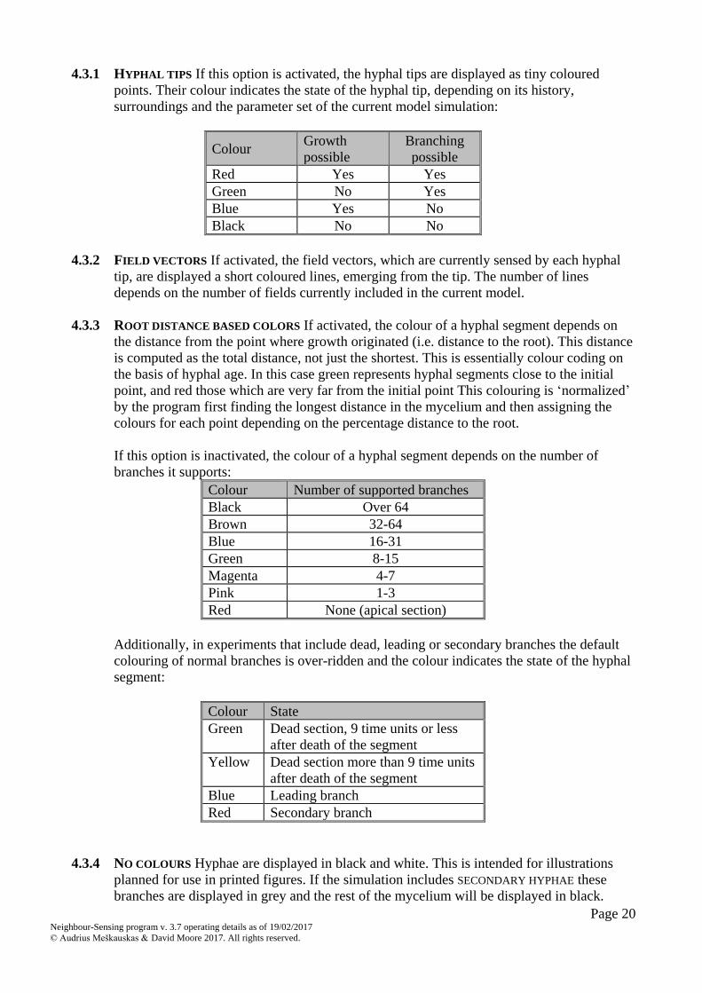
4.3.1 HYPHAL TIPS If this option is activated, the hyphal tips are displayed as tiny coloured

points. Their colour indicates the state of the hyphal tip, depending on its history,

surroundings and the parameter set of the current model simulation:

Colour Growth

possible

Branching

possible

Red Yes Yes

Green No Yes

Blue Yes No

Black No No

4.3.2 FIELD VECTORS If activated, the field vectors, which are currently sensed by each hyphal

tip, are displayed a short coloured lines, emerging from the tip. The number of lines

depends on the number of fields currently included in the current model.

4.3.3 ROOT DISTANCE BASED COLORS If activated, the colour of a hyphal segment depends on

the distance from the point where growth originated (i.e. distance to the root). This distance

is computed as the total distance, not just the shortest. This is essentially colour coding on

the basis of hyphal age. In this case green represents hyphal segments close to the initial

point, and red those which are very far from the initial point This colouring is ‘normalized’

by the program first finding the longest distance in the mycelium and then assigning the

colours for each point depending on the percentage distance to the root.

If this option is inactivated, the colour of a hyphal segment depends on the number of

branches it supports:

Colour Number of supported branches

Black Over 64

Brown 32-64

Blue 16-31

Green 8-15

Magenta 4-7

Pink 1-3

Red None (apical section)

Additionally, in experiments that include dead, leading or secondary branches the default

colouring of normal branches is over-ridden and the colour indicates the state of the hyphal

segment:

Colour State

Green Dead section, 9 time units or less

after death of the segment

Yellow Dead section more than 9 time units

after death of the segment

Blue Leading branch

Red Secondary branch

4.3.4 NO COLOURS Hyphae are displayed in black and white. This is intended for illustrations

planned for use in printed figures. If the simulation includes SECONDARY HYPHAE these

branches are displayed in grey and the rest of the mycelium will be displayed in black.



When you reset a colour choice after using the NO COLOURS option you should choose

STANDARD FRONT VIEW to restore the mycelium to its default colours as well as default

orientation.

4.3.5 STANDARD FRONT VIEW Turns the mycelial view angle to the front view.

4.3.6 REPAINT Repaints the mycelia (Java™ sometimes fails to do this automatically).

4.4 MODEL MENU

The MODEL MENU controls the simulation process and model parameters.

4.4.1 RESTART restarts the development from the single hyphal tip. This is the menu equivalent

of the START NEW button and it DISCARDS the current simulation.

4.4.2 PAUSE (or CONTINUE) suspends or resumes the current simulation.

4.4.3 SUBSTRATES… opens the SUBSTRATE MANAGER panel (referred to above, section 3.11,

and detailed below). The SUBSTRATE MANAGER PANEL allows the user to add attractive or

inhibitory substrates. It contains the following controls:

4.4.3.1 RETURN TO MAIN WINDOW returns to the main simulation window.

4.4.3.2 SIZE input field specifies the radius of the substrate. The current version supports

spherical substrates only. The hyphae can enter inside the substrate (subject to the

parameters chosen).

4.4.3.3 POSITION input fields specify the centre of the spherical substrate, (X, Y and Z co-

ordinates), in the same program-conditional units in which the whole mycelium is

measured.

4.4.3.4 NEGATIVE TROPISMS (INHIBITORY SUBSTRATE) check box indicates that the

hyphae will avoid this substrate rather than trying to get closer to it. Inhibitory

substrates are shown in red, whilst attractive substrates (that cause positive

tropisms) are shown in green.

4.4.3.5 ATTRACTIVENESS specifies the attractive force of the substrate, in relative units. If

the current model supposes that the autotropic field is generated by hyphal tips

only, this number indicates how much the field of the substrate is stronger than the

field of the single hyphal tip. If the autotropic field is generate by the whole

mycelia, this number indicates how much the field of the substrate is stronger than

the field of the hyphal section with the length, defined as “charge unit length” in

the NEIGHBOURHOOD section of the model parameters.

4.4.3.6 REMOVE ALL SUBSTRATES removes all substrates from the model.

4.4.3.7 REMOVE SELECTED removes the substrate(s) you select by highlighting with your

mouse.

4.4.3.8 CHANGE SELECTED updates the properties of the selected substrate to the values of

the input fields described above.



4.4.3.9 ADD NEW Enables you to add a new substrate with the properties that you specify

in the input fields.

The substrate list, which takes up the majority of this panel, shows all substrates currently

present in the model simulation. Substrates in this list can be selected with your mouse for

modifying and removing. Substrates can be modified at any time during simulations. The

substrate information is stored in mycelia.xml files together with other mycelial data.

4.4.4 OPTIONS opens the model parameter panel (explained in detail in section 3, above).

4.4.4.1 The PARAMETER PANEL sets the model parameters. The model supports three

hyphal types (STANDARD, LEADING and SECONDARY). Each group has its separate

independent parameter set. In the top right corner it is possible to choose the

current parameter group. The last tab in this group (SUMMARY) displays a short

non-redundant summary of the complete model parameter set. It is used for

documenting the work.

4.4.4.2 The model parameters for each hyphal type are also classified into categories

(TROPISMS, GROWTH AND BRANCHING, NEIGHBOURHOOD, AGE/LENGTH LIMITS,

DESTRUCTOR and COMMENTS).

4.4.4.3 The button MAKE THIS PAGE IDENTICAL makes the currently visible parameter

setting valid for all hyphal types.

4.4.4.4 The button ALL IDENTICAL overrides all settings for other hyphal types with

settings for the currently selected hyphal type.

4.4.4.5 At the bottom of the panel there are buttons for loading (LOAD PARAMETERS) and

storing (SAVE PARAMETERS) the model parameters. The parameters are also

automatically stored when saving the whole mycelium in .mycelia.xml files.

4.4.5 ROBOT Activates the animation robot. Immediately on choosing this option you will be

presented with a file management dialogue to choose the folder and filename of the

‘AutoDoc’ robot file in which your manipulations will be recorded (they will be saved as a

TXT format file). At the same time, some new control options appear at the bottom of the

main window. When you’ve made your choice of path and name of the file in which the

manipulations will be logged you will have access to the new controls. The new panel

contains controls to alter some model parameters manually and interactively. These

alterations can be recorded (in the ‘AutoDoc’ robot file). Later, you can rerun the

simulation and replay the automated parameter alterations so that parameters are

automatically changed during the new simulation in the same way as they were modified by

the operator during the original simulation (when they were recorded). At the start of the

replay process you will be prompted for the file name where the original alterations were

recorded.

The robot control panel consist of four parameters. Each parameter has a checkbox that

activates its scroll bar slider control on the robot control panel. If this box is unchecked, the

value for the corresponding parameter will be taken from the model options panel in the

usual way and NOT FROM THE ROBOT PANEL.



To the right of the checkbox is a short label, naming the parameter and its current value.

The value is changed by sliding the scroll bar located adjacent to this text. The control

parameters are:

4.4.5.1 ANGLE The angle of the plagiogravitropic reaction. This parameter only has effect

if the gravitropic reaction is supposed in the current model.

4.4.5.2 AUTOTROPISM b The long range positive autotropism (used to force hypha to join

together).

4.4.5.3 +/- GALVANOTROPISM The positive-negative galvanotropism, forcing hyphae to

grow at a right angle (90°) in relation to each other.

4.4.5.4 || GALVANOTROPISM The parallel galvanotropism, which forces hyphae to grow in

parallel, forming stems and mycelial cords.

4.4.5.5 The checkbox ROBOT, at the extreme bottom right of the panel, activates the

automatic parameter alteration FOR THE REPLAY PROCESS. After selecting this

checkbox you will be prompted for the file where alterations were previously

recorded.

IMPORTANT: you must ensure that the parameter set(s) for the hyphal category(ies) you

are attempting to manipulate DO have the appropriate parameters specified and activated.

These check boxes on the ROBOT panel only activate manual manipulation. You can

twiddle the ‘gravitropic reaction’ scroll bar as much as you like, but if you’ve not activated

gravitropism on THE DETAILS…> TROPISMS window for the appropriate hyphal category

(Standard, Leading and/or Secondary) then nothing can happen.

[If you just want to give the animation robot a try, we suggest you use the <CONUS> sample

parameter set. This has a 45 gravitropic angle setting in its parameters and usually

produces a conical fan of cyberhyphae. You can manipulate the gravitropic angle setting

with the scroll bar and change the cone into…well, anything you like, really.]

When you want to repeat the manipulations you just check the check box labelled ROBOT

and you will be presented with a file management dialogue to choose the folder and

filename of the robot file containing your manipulations. Once you’ve loaded this file and

resumed the visualisation, all of your manipulations will be repeated for you on a timescale

of program time units.

BUT THERE’S MORE. Remember that as the replay is proceeding you can pause the

visualisation at any time in order to slice it, re-scale it, rotate it, and/or save it. So if you’ve

produced a structure of particular interest you can generate all sorts of illustrations of its

development. And you can always re-run it again if you later think of something you should

have examined at a different scale, or from a different angle.

BUT THERE’S EVEN MORE. If you have produced a structure of particular interest you will

really want a visual record of the parameter changes that generated it. Well, remember that

the ‘AutoDoc’ robot file in which your manipulations are recorded is saved as a TXT

format file. The data in that file is actually formatted as a table – the first column = time (in

program time units) when the alteration was made; second column = angle of gravitropic

reaction; third column = level of long-distance autotropic reaction; fourth column = level of



parallel galvanotropic reaction; fifth column = +/- galvanotropic reaction. This text file is

tab-delimited and can be imported into graphical programs (like Excel, MathCad, FigP,

etc.) as data for generating graphs and charts of the parameter variations to match with your

illustrations of the developing visualisation.

…AND FINALLY: you can edit the robot file manually with a TEXT editor (like Notepad). So

you could manually change the timings of the manipulations, for example; or cut and paste

different manipulations together. There’s power in them ROBOT files!

4.4.6 HELP MENU: This currently provides a list of the program keys for running in console

mode.

APPENDIX 1

Using more than one processor

CALLING FUNGIMEDIA_3D.JAR FROM THE COMMAND LINE

FungiMedia_3D.jar is a cross platform Java™ application, able to run on any computer supporting

Java™ 1.4 or compatible. Depending on the platform and your purpose, you may need to run this file

from a command line. On most supercomputers, this is the only way to run the program.

The program itself is called by the following command:

java –jar FungiMedia_3D.jar –f ./taskFile.mycelia.xml –c other keys

The following keys are supported

–f file specifies the task file that is usually prepared to run the program under Windows or other

graphic environment.

-c Blocks the programs graphic user interface. The key is mandatory in batch mode where the

interaction with the user is not possible. It can also be used to run a prepared task under

Windows, which results in faster execution.

-save interval Specifies the interval, in program time units, for saving the current situation in a

standard task file. –save 1 is used to create sets that can be later converted into animations. If

this is not planned, it is better to use larger interval values, as saving takes execution time. The

default value is 10.

-until time Specifies the time (in program time units, not the absolute time) to terminate the program.

It is used when we wish to limit how long the simulation should continue.

-r file Specifies (if required) the robot file, containing changes of adjustable parameters.

-output folder Specifies the folder where results must be written. By default, results are written to the

folder from where the program was started.

-p number_of_processors Specifies the expected number of processors on a multiprocessor computer.

It must be equal to or a little larger than the actual number of processors available for use, but

too large a value slows the execution. The program cannot use more processors than are

specified with this key.



APPENDIX 2

Animations There are two ways to generate animations with the Neighbour-Sensing program. One is to activate an ANIMATION ROBOT

(detailed in section 4.4.5 of the Neighbour-Sensing Manual) that records your use of the parameter controls as you modify

the visualisation by manual interaction. This saves a record of the parameter changes you make and allows you to re-run a

visualisation at a later date (using the Neighbour-Sensing program) with exactly the same timing and sequence of

parameter changes. However, each time you run the robot you are creating a new visualisation with a new population of

hyphal tips, so there will be some ‘natural variation’. The combination of a pre-saved file of parameter settings and an

animation robot file of parameter settings is analogous to a living organism’s combination of genome and developmental

programme. The ANIMATION ROBOT is described above and we will not explain it further here.

The second animation technique is to use the Neighbour-Sensing program to generate a series of frames for a digital

movie. The frames can then be used by a suitable graphics program to create an AVI-format movie which can be viewed

independently of the Neighbour-Sensing program. This approach is simply a digital video record of one particular

visualisation, but it can be incorporated into your presentations and displays just like any other digital video movie. We

will describe this approach now.

Making digital video records We think we should start this section with the warning that we can generate some VERY LARGE files using this approach.

We are talking GIGAbytes here, even for a modest video. We think they’re really rather nice, and well worth the disk

space. Just the thing for the family to watch after dinner instead of the annual Christmas showing of ‘The Great Escape’,

but we must warn you that if you don’t have a capacious hard disk then you need to think carefully about your tactics.

The basic process is as follows:

Use the WRITE CHECKPOINT TO option on the FILE menu (section 4.1.4, above) to generate a regular series of

XML files as a visualisation progresses;

Use our independent conversion program (called Animator) to convert the XML files to JPG format;

Use a third-party graphics environment (we suggest John Ridley’s MakeAVI, detailed in Appendix 3 below) to

merge all the JPG files into an AVI file.

So let’s go. Choose the option WRITE CHECKPOINT TO on the FILE and you will be presented with a file management

dialogue to choose the (pre-existing) folder in which the XML files will be saved. Then, as soon as you resume the

visualisation, the program will save the XML files into that folder. These can be converted into animations later. To stop

saving the XML files it is best to pause the visualisation, and then exit the program. If you exit without pausing you may

find that the final frame is not fully completed. NOTE: the default arrangement is for XML files to be saved after each 10

iterations (that is at 10 program time unit intervals). The timing can be adjusted by editing the value in the SAVE AT

EACH… box in the file management dialogue. For ‘real-time’ videos, save your XMLs every iteration. Enter any value

greater than 1 in the SAVE AT EACH... box and the video will run faster than the original simulation. Saving XMLs every 50

iterations is useful for logging the progress of complex visualisations on an untended computer or supercomputer.

We have a separate program called Animator which will convert the XMLs you have just generated into JPG files. The

installer package for Animator can be downloaded from our website; installation is described below, for the moment we

will assume Animator is installed on your machine. Launch Animator; the start-up screen is very similar to the main

Neighbour-Sensing program:



But we must emphasise here that changing the size of this window regulates the size of the generated JPG graphics, so

size this window according to your plans for the final video.

Controls around the Animator window are like those around the Neighbour-Sensing program window: sliders across the

top control the scale of the display, and to rotate the image around vertical and horizontal axes. At right is a slider for

positioning the image vertically, and at bottom a slider for positioning the image horizontally in the field of view. The

bottom frame carries the main Animator controls.

At bottom left of the Animator window is a button labelled OPEN; ‘pressing’ this brings up a file management dialogue

box that enables you to select the folder in which you saved the XML files (previous paragraph).

When you Open that folder the number of files it contains is reported at bottom left of the Animator window. The slider

that occupies most of the bottom margin of the Animator window can be used to navigate through the images represented

by the XML files in the collection. The ‘scale’ of the slider becomes a horizontal ‘file list’ and by moving the pointer you

are choosing which of the images to display in the main dataspace window.

We recommend that you ‘slide’ to the last of your images (which we assume will be the largest) and then size the window

to frame that nicely. Such a strategy will ensure that the window size of the animation is optimised.

‘Click’ on the button labelled PLAY and Animator will run through your images, playing the animation it would produce so

that you can check it, and maybe modify the view. Remember, you are viewing a 2-dimensional image of a 3-dimensional

simulation; you might improve that 2-dimensional image by rotating (and/or changing the scale of) the 3-dimensional

simulation using the controls along the top of the Animator window.

The rate of progress of this process is not the same as the eventual video because this ‘rehearsal’ is very dependent on the

speed of your hard disk (because the XML files are being read in succession) and on the speed of your processor (because

the XML files are being rendered into images in succession). A second click on PLAY will stop the run through.

When you are satisfied with the ‘rehearsal’ you can ‘press’ the small button numbered 1 (alongside the OPEN button) and

this will open a file management dialogue which will show you your collection of XML files so you can choose which one

will start the digital video.

Then check the check box labelled WRITE IMAGES at bottom right of the Animator window. Now the images will be

written to disk when you ‘press’ (and hold) the PLAY button. You can pause the writing process at any time by releasing

the Play button. While paused, you can alter the image views (scale, rotation etc.), then ‘press’ PLAY again and writing will

resume from where it left off. When the process is completed you will have a folder called images (within the folder from

which Animator was run) which will contain a set of JPG files corresponding to your original set of XML files.

The next stage is to combine this collection of JPGs into an AVI digital video. There are many ways of doing this. What

we’re using at the moment is a freeware program called MakeAVI (see Appendix 3) and for the rest of this description we

will assume you will use this.

Run MakeAVI.exe and then choose ADD FILES, navigate to your images folder containing your JPGs and select all of them

using Ctrl-A. The file names will then be loaded into MakeAVI’s main window.

MakeAVI gives you some options to manipulate and arrange the files (which will be the frames in your video), but you’ve

probably done all you need to do in Animator. The only remaining option to consider on this screen is the frame rate. High

values may create unnecessary difficulties for your hard drive in reading the frames, so we suggest using 8 frames per

second.

‘Press’ BEGIN to start the process. You first get a file management dialogue in which you specify the filename and folder

for your AVI file, then ‘press’ SAVE and up will come a feedback box asking which video format you wish to save to. The

range of compression formats offered depends on the digital video codecs on YOUR computer. At the moment, we’re

recommending ‘Full Frames (Uncompressed)’ even though it can generate HUGE files. This is our recommendation

because the cyberhyphae in our images are so fine that they can be lost when the image is put through the compression

codecs we have tried so far. You may have better experience with more recent codecs. Make your choice, ‘press’ OK and

your video will be constructed.

Now you have your video you just have to double click on the file name and Windows will launch your multimedia

software so you can enjoy it. You could send it to your friends as a video greetings card.

Don’t blame us if they think you’re nerdy.

Download and install Animator

The program is distributed as a freeware .msi file you can download from our website at this URL:

www.davidmoore.org.uk\CyberWEB\Downloads

http://www.davidmoore.org.uk/CyberWEB/Downloads



Download the .msi file named animator.msi. Then navigate (in File Explorer) to the folder in which this file was saved and

double-click on the file name to run the file [OR right-click on the animator.msi file name and choose ‘Install’ from the

menu that appears].




We expect you’ll be an old hand at this now, so you’ll already be positioning your cursor in the edit window and typing the

address of the USB drive on which you want to install Animator. I’ll assume your USB drive will be drive E: (you may have

to Browse to use File Explorer to confirm that) and suggest you type E:\f3d\animator into that edit window. With that done,

click on the ‘Next >’ button and the Installer will do everything for you. It will keep you informed of progress and announce

when it’s finished.

When the installation is complete, use File Explorer to Browse to, and look inside, the folder you’ve just created (\animator\)

and (again, as an old hand) you’ll not be surprised to find it contains folders called jars, jre-animator and sources, and a

.swidtag file with a ridiculously long file name. Again, the folder you need to go to launch Animator is the one called jars;

which contains a single ‘executable jar file’ called animator.jar that will launch the Animator program.

Before you do launch we’ll repeat our recommendation that you create a shortcut to animator.jar to save yourself the hassle

of navigating through all these folders to launch it. Highlight animator.jar in the folder window, then right- click and choose

‘Create shortcut’ from the menu that appears. The shortcut will appear in the same window beneath animator.jar, and you

can then drag-and-drop the newly created shortcut from that folder window to your Desktop, where it will be served with a

‘steaming cup of java’ icon.

Before you launch Animator for the first time, read on, because we’ve also given you some ready-made XML and JPG files

that you can use to test out Animator and MakeAVI.

The file folder called sources that you’ve just installed is an archive containing the program ZIP files animator.zip and

neighbour-sensing_model.zip), which hold all the .java files for those programs, as well as the usual .txt copy of the

GNU General Public License [https://www.gnu.org/licenses/gpl.html] under which this software is distributed. But it

also contains a ZIP file called Animations.zip, which contains some additional goodies.



When you extract this ZIP file you will get seven folders containing many hundreds of ready-made XML files from the

Neighbour-Sensing simulator:

You can use these files to experiment with Animator; and it doesn’t matter what you do to these files, you can always

replace them by re-extracting the ZIP file.

ALSO…

The extracted folder called alt_Coprinus contains BOTH a folder with 924 XML files AND one containing 923

corresponding JPG files.

You can use the ready-made JPG files to test out Make AVI.



APPENDIX 3

MakeAVI (version 0.11 update of 9/4/2013)

Developed by John Ridley

Available from: https://sourceforge.net/projects/makeavi/ (last checked February 2017)

John Ridley writes: This is a quick and dirty app that I wrote because I wanted to do some work with creating time-

lapse movies. For that particular project, I set up a digital camera to take a picture every 10 seconds for several hours,

then I wanted to string the JPGs together into an AVI, and do any video work from there.

This program allows you to do that sort of thing. It will read JPGs, as well as PNG, BMP, and several other formats (no

GIF, and don’t bother begging). The program is very simple and easy to understand. The instructions are all in the

README.TXT file. Here’s a screenshot in case you’re into those things:

Introduction

The core of the AVI generation is the Microsoft/Windows AVI API. Wrapped around that is a thin wrapper, which I

found at www.codeguru.com, but it may be from a Microsoft sample app, I don’t know. The image loading end is

handled by the FreeImage library, which is currently at http://www.6ixsoft.com/. It can handle many different image

types, but not GIF. GIF is patent burdened and will not be supported, so don’t bother asking.

License: MakeAVI is free software, licensed under the GPL (GNU General Public License). Significant portions of

MakeAVI (specifically, the FreeImage library) are also licensed under the GPL. For more information, please read the

LICENSE.TXT file that should have come with this release. If you do not have a copy of this file, you can find it at

http://www.gnu.org/licenses/gpl.txt

Installation

Unzip all this stuff into one directory. Run MAKEAVI.EXE. There, it’s installed. If you want to get cute, right click on

MakeAVI, hit “Create shortcut” and drag the shortcut onto your desktop.

Using MakeAVI

You want to select all your images into the list on the left. Use the “Add Files” button to choose your files. Use the

“Add Files”, “Delete File”, “Sort Files”, and “Move file Up/Down” buttons to get the images in the order you want

them. Any image that is selected on the left will be previewed in the middle. If it isn’t previewed properly, then the

program is unable to read the image (can’t access the file, or the file is corrupt, or something).

Cropping

All the images have to be the same size to go into an AVI file If you have images of varying sizes, or you have junk at

the edge that you want to eliminate from the final AVI, you can use the “Cropping” interface at the bottom. Check the

“Crop to” box, and select the size you want the final images to be cropped to in the boxes to the right. NOTE that the

https://sourceforge.net/projects/makeavi/



original images are NOT cropped on disk, they are only cropped after they’re loaded, and before they’re added to the

AVI.

NOTE that currently, images are cropped towards the centre, you can’t select where the cropping occurs. As an aid to

filling in these values, if you add new images to the list, the size of the last image added is put into those edit boxes.

Also, you can double click on any image in the list at any time and the size of that image will be copied in to the boxes.

Ready to go...

When you’ve gotten the images all in order, input your frame rate in the box provided; when you play the final AVI file,

that many images will be played per second.

Then, press the “Begin!” button. The feedback box will be displayed, and you will be asked which video format you

wish to save to. I won’t try to talk about video formats here, except for a few observations:

If you will be continuing to work with the video, perhaps encoding it to other formats, then you may want to use

“Uncompressed” – though that generates HUGE files. In general time lapse stuff is not that big, so your file will

probably only be a few gigabytes, so this is not a bad choice, but it should NOT be used for the final product; the data

rate is so high that most computers will not be able to play the video smoothly.

If you are going for a final AVI product, Indeo 4.5 or higher is a good choice, since everyone either has it or can get the

codec automatically when they start to play the video under Windows media player.

Possible future enhancements:

Cropping other than from the center

Resizing images

Fixing support for a few codecs that don’t work for some reason.

© John Ridley 2002

neighbour-sensing version 3 - david moore€¦ · our website offers for download a short video (it...

Documents