Negative magnetoresistance without well-defined chiral-ity in the Weyl semimetal TaP

Frank Arnold1 ∗, Chandra Shekhar1 ∗, Shu-Chun Wu1, Yan Sun1, Ricardo Donizeth dos Reis1,

Nitesh Kumar1, Marcel Naumann1, Mukkattu O. Ajeesh1, Marcus Schmidt1, Adolfo G. Grushin2,

Jens H. Bardarson2, Michael Baenitz1, Dmitry Sokolov1, Horst Borrmann1, Michael Nicklas1,

Claudia Felser1, Elena Hassinger1 †, & Binghai Yan1,2 †

1Max Planck Institute for Chemical Physics of Solids, 01187 Dresden, Germany

2Max Planck Institute for the Physics of Complex Systems, 01187 Dresden, Germany

∗ These authors contributed equally to this work.

Weyl semimetals (WSMs) are topological quantum states 1 wherein the electronic bands lin-

early disperse around pairs of nodes, the Weyl points, of fixed (left or right) chirality. The re-

cent discovery of WSM materials 2–7 triggered an experimental search for the exotic quantum

phenomenon known as the chiral anomaly 8, 9. Via the chiral anomaly nonorthogonal electric

and magnetic fields induce a chiral density imbalance that results in an unconventional neg-

ative longitudinal magnetoresistance 10, the chiral magnetic effect. Recent theoretical work

suggests that this effect does not require well-defined Weyl nodes 11–13. Experimentally how-

ever, it remains an open question to what extent it survives when chirality is not well-defined,

for example when the Fermi energy is far away from the Weyl points. Here, we establish

the detailed Fermi surface topology of the recently identified WSM TaP 14 via a combination

of angle-resolved quantum oscillation spectra and band structure calculations. The Fermi

1

arX

iv:1

506.

0657

7v2

[co

nd-m

at.m

trl-

sci]

4 F

eb 2

016

surface forms spin-polarized banana-shaped electron and hole pockets attached to pairs of

Weyl points. Although the chiral anomaly is therefore ill-defined, we observe a large negative

magnetoresistance (NMR) appearing for collinear magnetic and electric fields as observed in

other WSMs 15, 16. In addition, we show experimental signatures indicating that such lon-

gitudinal magnetoresistance measurements can be affected by an inhomogeneous current

distribution inside the sample in a magnetic field 17. Our results provide a clear framework

how to detect the chiral magnetic effect.

In a semimetal the conduction and valence bands touch at isolated points in the three-

dimensional (3D) momentum (k) space at which the bands disperse linearly. Depending on whether

the bands are nondegenerate or doubly degenerate, such a 3D semimetal is called a Weyl semimetal

(WSM) 1, 18, 19 or a Dirac semimetal (DSM) 20–22, respectively. Correspondingly, the band touching

point is referred to as a Weyl point or a Dirac point. The Dirac point can split into one or two pairs

of Weyl points by breaking either time-reversal symmetry or crystal inversion symmetry. At ener-

gies close to the Weyl points, electrons behave effectively as Weyl fermions, a fundamental kind of

massless fermions that has never been observed as an elementary particle 23. In condensed-matter

physics, each Weyl point acts like a singularity of the Berry curvature in the Brillouin zone (BZ),

equivalent to magnetic monopoles in k space, and thus always occur in pairs with opposite chirality

or handedness 24. In the presence of nonorthogonal magnetic (B) and electric (E) fields (i.e., E·B is

nonzero), the particle number for a given chirality is not conserved quantum mechanically, a phe-

nomenon known as the Adler-Bell-Jackiw anomaly or chiral anomaly in high-energy physics 8, 9, 23.

In Weyl semimetals, the chiral anomaly is predicted to lead to a negative magnetoresistance (MR)

2

due to the suppressed backscattering of electrons of opposite chirality 10, 25.

Theoretically, the chiral anomaly strictly appears only, when the chirality is well-defined, i.e.,

the Fermi energy is close enough to the Weyl nodes such that the two Fermi surface pockets around

Weyl nodes of a pair of opposite chirality are independent 10. Observing the chiral-anomaly-

induced MR requires that the applied magnetic field and current be as parallel as possible, as

otherwise the negative MR will easily be overwhelmed by the positive contribution of the Lorentz

force. In addition to a negative MR, the chiral anomaly is predicted to induce an anomalous Hall

effect 19, 26–28, nonlocal transport properties 29, 30 and sharp discontinuities in ARPES signals 31 in

WSMs.

The discovery of different WSM materials has stimulated experimental efforts to confirm

the chiral anomaly in condensed-matter physics. Recently, negative MR has been reported in two

types of WSMs: WSMs induced by time reversal symmetry breaking, i.e., Dirac semi metals in

an applied magnetic field, for example Bi1−xSbx (x ≈ 3%) 32, ZrTe5, 33 and Na3Bi 34, and the

inversion-asymmetric WSMs TaAs 15, 16, NbP, 35 and NbAs 36. However, a clear verification of

whether the Fermi surface topology supports the chiral anomaly or not, is still lacking in most of

the above systems.

In the non-centrosymmetric WSM of the TaAs family two types of Weyl nodes exist at dif-

ferent positions in reciprocal space 3, 4 and at different energies. Therefore, the Weyl electrons

will generally coexist with normal electrons. Small changes of the Fermi energy by doping or

vacancies can in principle change the topology of the Fermi surface significantly due to the small-

3

ness of the carrier density. Therefore, the Fermi energy and resulting Fermi surface topology in

a crystal have to be known precisely when linking the negative MR to the chiral magnetic effect.

Extensive angle-resolved photoemission spectroscopy (ARPES) measurements in the TaAs family

have shown the existance of Fermi arc surface states and linear band crossings in the bulk band

structure in all four materials 5–7, 14, 37. However, because of the insufficient energy resolution (¿ 15

meV 14), these measurements are not able to make any claims about the presence or absence of a

well-defined chirality at the Fermi level. Quantum oscillation measurements have the advantage of

an meV resolution of the Fermi energy level.

In this work, we reconstruct the 3D Fermi surface of TaP by combining sensitive Shubnikov–

de Haas (SdH) and de Haas–van Alphen (dHvA) oscillations with ab initio band structure calcula-

tions reaching a good agreement between theory and experiment. We reveal that the Fermi energy

is such that electron and hole Fermi surfaces contain pairs of Weyl nodes. Although the chiral

anomaly is not well-defined, a large negative MR is measured. We discuss possible explanations

for this result considering also the current distribution in our samples 38.

We synthesized high-quality single crystals of TaP by using chemical vapor transport re-

actions and verified TaP as a noncentrosymmetric compound in a tetragonal lattice (space group

I41md, No. 109). The temperature-dependent resistivity exhibits typical semimetallic behavior.

For more details see the Supplementary Information (SI).

The Fermi surface topology of TaP was investigated by means of quantum oscillations. Typ-

ically, for a semimetal with light carriers and high mobility, such as bismuth 39, prominent oscil-

4

−90 −60 −30 0 30 60 90 120101

102

θ (deg)

[110] [001] [100] [110]

F(T

)

A C

B

SQUIDTorqueResistivity

E (Theory)H (Theory)

TaP

γ

γ'

γ

γ"

B (T)0 6 12 14

τ(ar

b. u

nits)

B ǁ c

B ǁ a

10842

B (T)

ρ xx

(mΩ

cm)

4

8

120o

10o

20o

30o

40o

50o

60o

70o

80o

90o

B ǁ c

0 6 12 1410842

B ǁ c B ǁ a

β

α

δ

α

α"

δ

δ"

Figure 1: Quantum oscillations and angular dependence of oscillation frequencies in TaP.

A. Shubnikov-de Haas oscillations in resistivity for different angles in steps of 10. B. Quantum

oscillations from magnetic torque measurements for the same angles. C. Full angular dependence

of the measured and theoretical quantum oscillation frequencies. Open and closed symbols refer to

SdH and dHvA data of five different samples from two different batches. Lines show the extremal

orbits calculated from the banana-shaped 3D Fermi surface topology given in Fig. 3 (solid lines

for the pockets lying in the tilting plane of the magnetic field, dashed lines for the pockets lying

perpendicular to it).

lations appear in all measurable properties sensitive to the density of states at the Fermi energy.

Here, we measured Shubnikov-de Haas (SdH) oscillations in transport (Fig. 1A) and de Haas-van

Alphen (dHvA) oscillations in torque (Fig. 1B) and magnetization (Fig. 2A) for different field

orientations. These oscillations are periodic in 1/B and their frequency (F ) is proportional to the

extremal Fermi surface cross section (Ak) that is perpendicular to B following the Onsager relation

5

F = (Φ0/2π2)Ak, where Φ0 = h/2e is the magnetic flux quantum and h is the Planck constant.

Figure 1A shows the resistivity as a function of the magnetic field for different field orientations.

When the electric current and magnetic field are perpendicular (B||c), the magnetoresistance is very

high as typical for other WSM (for example ref. 40) and normal semimetals 41, 42. This implies a

very high mobility of the charge carriers.

Figure 1B depicts the magnetic torque oscillations for the same field orientations. Figure 2A

represents the magnetic dHvA oscillations in the magnetization as a function of the inverse mag-

netic field and their corresponding Fourier transform (Fig. 2B) for B||c. The observable fundamen-

tal frequencies from these measurements are Fα = 15 T, Fβ = 18 T, Fγ = 25 T, and Fδ = 45 T. The

frequencies are consistent within the error bar (given in Table I in the SI) for all three measurement

techniques and different sample batches. This indicates that all samples have a similar chemical

potential to within 1 meV. Additionally, we can conclude that the resistivity measurements are sen-

sitive to the bulk Fermi surface as well. For B||a the main frequencies are Fα = 26 T, Fγ = 34 T,

Fγ′ = 105 T Fδ = 147 T, and Fγ′′ = 320 T clearly indicating anisotropic 3D Fermi surface pockets.

For most of the detected oscillation frequencies, we derive their cyclotron effective masses (m∗) of

the carriers by fitting the temperature dependence of the oscillation amplitude (insert of Fig. 2B)

with the Lifshitz-Kosevich formula (see Ref. 43 and the SI). The values of the effective masses are

m∗α = (0.021± 0.003)m0, m∗β = (0.05± 0.01)m0, and m∗δ = (0.11± 0.01)m0 for B||c, whereas

they are a factor of 4–10 greater for B||a with m?γ = (0.13 ± 0.03)m0, m?

γ′ = (0.35 ± 0.03)m0,

and m∗δ = (0.4 ± 0.1)m0, where m0 is the mass of a free electron (see Table I in the SI). These

values are small and comparable to the effective masses in other slightly doped Dirac materials

6

Figure 2: Quantum oscillations, effective masses, carrier density and mobility. A. Quantum

oscillations in the magnetization as a function of the inverse field for T = 1.85 K. B. FFT of the

curve in A. C. Hall resistivity of sample S1 for different temperatures as indicated and the fits

with a two band model (dashed lines). D. Carrier concentration and mobility of the hole (H) and

electron (E) pockets as obtained by fitting the temperature-dependent Hall resistivity of samples

S1 and S3, which are labeled by triangles and diamonds, respectively. The gray-shaded areas

give the confidence intervals of the densities and mobilities. The blue and red dashed lines mark

the theoretical electron and hole densities based on the fitted quantum oscillation and DFT Fermi

surface. The hole mobility labeled by a star is determined from dHvA analysis.

7

such as Cd3As2 or graphene 44, 45 . These low masses, together with long scattering times are the

reason for the high mobility and the huge transverse magnetoresistances seen in semimetals.

8

Figure 3: 3D Fermi pockets and Weyl points. A. Fermi pockets in the first Brillouin zone at

the Fermi energy (EF ) detected in the experiment. The electron (E) and hole (H) pockets are

represented by blue and red colors, respectively. B. Enlargement of the banana-shaped E and H

pockets. The pink and green points indicate the Weyl points with opposite chirality. W1- and W2-

type Weyl points can be found insideE and close toH pockets, respectively. Green loops represent

some extremal E and H cross sections, corresponding to the oscillation frequencies measured,

Fα,β,γ,δ for H||c (see the text). C. Energy dispersion along the connecting line between a pair of

Weyl points with opposite chirality for W1 (left) and W2 (right). The deduced experimental EF

(thick dashed horizontal line) is 14 meV below the W2 Weyl points and 51 meV above the W1

Weyl points. D. Strongly anisotropic Weyl cones originating from a pair of W2-type Weyl points

on the plane of Fγ . Green and red Weyl cones represent opposite chirality.

9

To reconstruct the shape of the Fermi surface, the full angular dependence of the quantum

oscillation frequencies is measured and compared to band-structure calculations (Fig. 1C). The

exact position of the Fermi energy (EF ) is determined by matching the calculated frequencies

and their angular dependence to the measured ones (see the SI for more details). The best fit is

obtained when EF lies 5 meV above the ideal electron-hole compensation point, in agreement

with the resulting carrier concentration from the Hall measurements (Fig. 2C and D). Calculations

reveal two banana-shaped Fermi surface pockets at this EF , a hole pocket (H) and a slightly larger

electron pocket (E). These two pockets reproduce the angular dependence of the measured dHvA

frequencies with great accuracy (see lines in Fig. 1C and the Fermi surface in Fig. 3). E and H are

almost semicircular and are distributed along rings 3, 4 on the kx = 0 and ky = 0 mirror-planes in

the BZ. The rather isotropic frequencies Fα and Fγ result from a neck and extra humps (“head with

horns”) at the end of the hole pocket (see Fig. 3B). The splitting of all frequencies with field angles

departing from B||c in the (100)-plane is explained by the existence of four banana-shaped pockets

in the BZ, two for each mirror plane for both E and H pockets. The splitting of the frequency Fδ

seen in the experiment is not reproduced by the calculation. One possibility for this discrepancy is

that a waist may appear in the E-pocket at kz = 0.

The Berry phase for the largest β oscillations from our magnetization in Fig. 2A is trivial

(see SI). Additionally, in the dHvA experiment the mobility of the hole orbits (Fα and Fβ) was

extracted via the width of the Fourier transform peaks, which is given by the exponential decrease

of the oscillations with 1/B (the so-called Dingle term; see the SI). The deduced mobility is

µh = 3.2× 104 (±20%) cm2 V−1s−1 (star in Fig. 2D).

10

We extract information on the carrier density and mobility from field- and temperature-

dependent Hall measurements in sample S1 (full temperature range, Fig. 2C) and only at low

temperature in sample S3 from a different batch. We employ a two-carrier model (see Ref. 46) to

fit the Hall conductivity (σxy) by making use of the longitudinal conductivity at zero field (σxx)

as an additional condition (see the SI). As shown in the left panel of Fig. 2D, the carrier concen-

tration for both electrons and holes at low temperature is around n = (2 ± 1) × 1019 cm−3 with

an absolute error bar given approximately by the scattering of the data for different samples and

shown as a gray-shaded area. Although TaP is almost a compensated metal, the electron density

is slightly larger than the hole density for each sample at low temperature, in agreement with the

fact that EF lies 5 meV above the charge-neutral point determined from the Fermi surface topol-

ogy. The theoretical values of the carrier densities, given in Fig. 2D as dashed lines, are in good

agreement with the experimental data. Note that above 150 K the hole density becomes larger than

the electron density for sample S1. This inversion is reflected in the sign change of the high field

Hall resistivity (see SI) and is similar to the Hall effect observed in TaAs 15, 16 and NbP 35, 40. The

mobility of both carriers at low temperature lies in the range of µ = (2–5)× 104 cm2 V−1s−1, with

the hole mobility higher than the electron one. The high mobility indicates the very high quality of

the single crystals with only a few defects and impurities. The Hall mobility agrees well with the

mobility from dHvA measurements (the star in Fig. 2D).

The measured Fermi surface topology and carrier concentration described above converge

to the same statement that the Fermi energy EF of our samples is 5 meV above the ideal charge-

neutral point in the calculated band structure. This slight doping is not expected for a completely

11

stoichiometric sample. However, a slight appearence of defects/vacancies in this type of samples

is possible 47 and can explain this small shift of the Fermi energy. The consistency between exper-

iment and theory strongly suggests that this is the true Fermi surface of our TaP samples. We plot

the corresponding 3D Fermi surfaces from the ab initio calculations in Fig. 3. One can see that E

and H pockets are the only two pockets at the Fermi energy.

We investigate the Weyl points in the band structure. In the 3D BZ, there are twelve pairs of

Weyl points with opposite chirality: four pairs lie in the kz = 0 plane (labeled as W1) and eight

pairs are located in planes close to kz = ±π/c (where c is the lattice constant) (labeled as W2).

One can see that the W1 points are far below EF by 51 meV and are included in the E pocket.

The W2-type Weyl points are 14 meV above EF and are included in the H pocket. Such pairs of

W2 points merge slightly into the head position of the H pocket, leading to a two-horn-like cross

section (see Fγ in Fig. 3B). Energetically, they are separated by a 16 meV barrier along the line

connecting the Weyl points of a pair. We plot the energy dispersion of Weyl bands over the Fγ

plane in Fig. 3D. There are no independent Fermi surface pockets around the W2 Weyl points

and therefore the chiral anomaly is not well-defined. The Weyl cone is strongly anisotropic in the

lower cone region below the Weyl point.

Finally, we discuss the longitudinal magnetotransport properties of TaP. We measure the

longitudinal magnetoresistance of three samples from the same crystal batch where the current (I)

is along the crystallographic c (sample S2) and a (samples S1 and S4) axes, respectively. Figure 4A

and B represent the longitudinal magnetoresistance (MR? = [V −V (B = 0)]/V (B = 0) where V

12

Figure 4: Negative longitudinal magnetoresistance in TaP. A. Longitudinal MR? = [V −V (B =

0)]/V (B = 0) for B||I||c for different temperatures. B. Same for B||I||a. The temperatures are

the same as in A. C. Same for B||I||a and three pairs of contacts. The difference in the curves can

be explained by an inhomogeneous current distribution induced by the magnetic field (see text).

The contact geometry is shown in the inserts: panel B for S1 and S2, and panel C for S4. D.

Theoretical curves for S4 as in panel C. For details about the calculation see the text and the SI 51.

is the measured voltage drop with a fixed electric current) measured for the two crystallographic

directions. MR? is equal to the usual MR = [ρ− ρ(B = 0)]/ρ(B = 0) as long as the current flows

homogeneously in the sample. At 1.85 K, the MR? first increases slightly and soon drops steeply

from positive to negative values. The negative MR? is very robust with increasing temperature.

Note that the MR? is negative only in a very narrow window of θ ≤ 2 and becomes positive

otherwise (see SI). The small θ window of negative MR? is similar to that observed in Na3Bi 34. In

light of the given Fermi energy position in our crystals, it is not possible to link the negative MR?

to the chiral anomaly, simply because the former is not a well-defined concept when the Fermi

13

surface connects both Weyl nodes. Although this does not rule out the presence of a non-trivial

negative MR 11–13, we find that the observed negative MR? is strongly affected by the geometric

configuration.

This becomes apparent when we measure the longitudinal MR? for three different voltage

contact configurations on sample S4 as illustrated in Fig. 4C. A clear voltage decrease in magnetic

field is observed in pair V1, similar to the low temperature curves in Fig. 4A and B, whereas the

two other pairs, denoted V2 and V3, show a higher MR?. This points to an underlying inhomoge-

neous current distribution in the sample becoming important in high magnetic fields. As typical for

high mobility semimetals, TaP has a large transverse MR arising from the orbital effect, whereas

the longitudinal MR most likely stays of the same order of magnitude. For current contacts smaller

than the cross section of the sample, this leads to a field-induced stearing of the current to the di-

rection of the magnetic field, which is along the line connecting the current contacts when current

and magnetic field are parallel. This effect is known as “current jetting” 17, 38, 48–51. As a conse-

quence, a voltage pair close to this line (V3) detects a higher MR? than the intrinsic longitudinal

MR whereas a voltage pair far away from it (V1) detects a smaller MR? than the intrinsic one. This

effect is confirmed by calculations of the voltage distribution for sample S4, taking into account

the current jetting by following ref. 51 (see SI). Using the measured transverse MR and assuming a

field-independent intrinsic longitudinal MR, the model qualitatively reproduces the three observed

MR? curves without any free parameters (see Fig. 4D). Therefore, the field dependence of the

longitudinal measured voltage is largely induced by the strong transverse MR, if the current is not

homogeneously injected into the whole cross section of the sample.

14

In summary, we determined the Fermi surface topology of the inversion-asymmetric WSM

TaP. The Fermi surface consists of banana-shaped spin-polarized electron and hole pockets with

very light carrier effective masses. Despite the absence of independent Fermi surface pockets

around the Weyl points, an apparent negative longitudinal MR is detected. We show that in such

measurements, special care is needed to avoid a decoupling of the voltage contacts from the current

jet in longitudinal magnetic fields.

Methods

Single crystal growth. High-quality single crystals of TaP were grown via a chemical va-

por transport reaction using iodine as a transport agent. Initially, polycrystalline powder of TaP

was synthesized by a direct reaction of tantalum (Chempur 99.9%) and red phosphorus (Heraeus

99.999%) kept in an evacuated fused silica tube for 48 hours at 800 C. Starting from this micro-

crystalline powder, the single-crystals of TaP were synthesized by chemical vapor transport in a

temperature gradient starting from 850 C (source) to 950 C (sink) and a transport agent with a

concentration of 13.5 mg/cm3 iodine (Alfa Aesar 99,998%) 52. The orientation and crystal struc-

ture of the present single crystals were investigated using the diffraction data sets collected on a

Rigaku AFC7 diffractometer equipped with a Saturn 724+ CCD detector (monochromatic MoKα

radiation, λ = 0.71073 A). Structure refinement was performed by full-matrix least-squares on F

within the program package WinCSD.

Magnetization. The magnetism and magnetic quantum oscillations of TaP along the main

crystallographic axes were measured in a Quantum Design SQUID-VSM. The angular dependen-

15

cies were measured using the Quantum Design piezo-resistive torque magnetometer (Tq-Mag 53)

in a PPMS with installed rotator option. Magnetization and torque measurements were performed

on two large 4.4 and 21.7 mg TaP single crystals. The samples were mounted on the sample holder

and torque lever by GE varnish or Apiezon N grease and aligned along their visible crystal facets,

which was confirmed by X-ray diffraction measurements. The crystal alignment was verified by

photometric methods and showed typical misalignments of less than 2. SQUID magnetization

measurements were performed for static positive and negative magnetic fields up to 7 T in the

temperature range of 2 to 50 K. Magnetic torque measurements were performed up to 14 T in

the same temperature range. Here the sample is mounted on a flexible lever which bends when

torque is applied. The sample magnetization M induces a magnetic torque τ = M × B, which

bends the lever and can be sensed by piezo-resistive elements which are micro-fabricated onto the

torque lever. These elements change their resistance under strain and are thus capable of sensing

the bending of the torque lever. The unstrained resistance of these piezo-resistors is typically 500

Ω and can change by up to a few percent when large magnetic torques are applied. Measuring

quantum oscillations, however, requires a higher torque resolution. Thus the standard torque op-

tion was altered and extended by an external balancing circuit and SR830 lock-in amplifiers as

read-out electronic. This way a resolution of one in 107 was achieved. The magnetic torque was

measured for magnetic fields in the (100), (001) and (110)-plane in angular steps of 2.5 and 5.

Measurements were taken during magnetic field down sweeps from 14 to 0 T. The magnetic field

sweep rate was adjusted such that the sweep rate in 1/B was constant. The resultant magnetic

torque signals are a superposition of the sample diamagnetism, de Haas-van Alphen oscillation

16

and uncompensated magneto-resistance of the piezo-resistors. Due to the vector product of the

magnetization and magnetic field, this method can only be applied to samples with strong Fermi

surface anisotropy and is insensitive when the magnetic field and magnetization are aligned par-

allel, e.g. along the crystallographic c-direction in TaP. The quantum oscillation frequencies are

extracted from the measured resistivities and magnetizations by subtracting all back ground con-

tributions to those signals and performing a Fourier transformation of the residual signal over the

inverse magnetic field. The resulting spectra show the de Haas-van Alphen frequencies and their

amplitude.

Band structure calculations. The ab initio calculations were performed using density-functional

theory with the Vienna ab-initio simulation package 54. Projector-augmented-wave potential rep-

resented core electrons. The modified Becke-Johnson exchange potential 55, 56 was employed for

accurate band structure calculations. Fermi surfaces were interpolated using maximally localized

Wannier functions (MLWFs) 57 in dense k-grids (equivalent to 300× 300× 300 in the whole BZ).

Then angle-dependent extremal cross-sections of Fermi surfaces are calculated to compare with

the oscillation frequencies according to the Onsager relation.

Magnetoresistance measurement. Resistivity measurements were performed in a physical

property measurement system (PPMS, Quantum Design) using the DC mode of the AC-Transport

option. Samples with two different crystalline orientations, i.e., bars with their long direction par-

allel to the crystallographic a and c-axis, were cut from large TaP single crystals using a wire saw.

The orientation of these crystals was verified by x-ray diffraction measurements. A detailed analy-

17

sis of their crystalline orientations is given in the SI. The samples were named S1 (I||a), S2 (I||c),

S3 (I||a) and S4(I||a). The physical dimensions of S1, S2, S3 and S4 are (width × thickness ×

length) 0.42×0.16×1.1 mm3, 0.48×0.27×0.8 mm3, 0.5×0.2×3.0 mm3 and 0.79×0.57×3.2 mm3,

respectively. Contacts to the crystals were made by spot welding 25 micrometer platinum wire

(S1 and S2) or gluing 25 micrometer gold wire to the sample using silver loaded epoxy (Dupont

6838). The resistance and Hall effect were measured in 6-point geometry using a current of about

3 milliampere at temperatures of 1.85 to 300 K and magnetic fields up to 14 T. Crystals were

mounted on a PPMS rotator option. Special attention was paid to the mounting of the samples on

the rotator puck to ensure a good parallel alignment of the current and magnetic direction. The Hall

contributions to the resistance and vice versa were accounted for by calculating the mean and dif-

ferential resistance of positive and negative magnetic fields. Almost symmetrical resistivities were

obtained for positive and negative magnetic fields when current and magnetic field were parallel

showing the excellent crystal and contact alignment of our samples. Otherwise, the negative MR?

was overwhelmed by the transverse resistivity. In order to increase the sensitivity of the angular

dependent Shubnikov-de Haas measurements at low magnetic fields, external Stanford Research

SR830 lock-in amplifiers were used to measure the resistance and Hall resistance. Here typical

excitation currents of a 2 to 5 milliampere were applied at frequencies of about 20 Hz.

Acknowledgements We are grateful for Dr. L.-K. Lim, Prof. E. G. Mele, Prof. Z.-K. Liu, and Prof. Y.-L.

Chen, and Prof. S.-Q. Shen for helpful discussions. This work was financially supported by the Deutsche

Forschungsgemein- schaft DFG (Project No. EB 518/1-1 of DFG-SPP 1666 “Topological Insulators”, and

SFB 1143) and by the ERC (Advanced Grant No. 291472 Idea Heusler). AGG acknowledges insightful

18

discussions with D. Varjas and J. Moore. R. D. dos Reis acknowledges financial support from the Brazilian

agency CNPq.

Competing Interests The authors declare that they have no competing financial interests.

Correspondence Correspondence should be addressed to B. Yan (email: yan@cpfs.mpg.de) or E. Has-

singer (email: elena.hassinger@cpfs.mpg.de).

1. Wan, X. G., Turner, A. M., Vishwanath, A. & Savrasov, S. Y. Topological semimetal and

Fermi-arc surface states in the electronic structure of pyrochlore iridates. Phys. Rev. B 83,

205101 (2011).

2. Liu, Z. K. et al. Discovery of a Three-Dimensional Topological Dirac Semimetal, Na3Bi.

Science 343, 864–867 (2014).

3. Weng, H., Fang, C., Fang, Z., Bernevig, B. A. & Dai, X. Weyl Semimetal Phase in Noncen-

trosymmetric Transition-Metal Monophosphides. Phys. Rev. X 5, 011029 (2015).

4. Huang, S.-M. et al. A Weyl Fermion semimetal with surface Fermi arcs in the transition metal

monopnictide TaAs class. Nat. Comms. 6, 7373 (2015).

5. Lv, B. Q. et al. Experimental Discovery of Weyl Semimetal TaAs. Phys. Rev. X 5, 031013

(2015).

6. Xu, S.-Y. et al. Discovery of a Weyl fermion semimetal and topological Fermi arcs. Science

349, 613 (2015).

19

7. Yang, L. X. et al. Weyl Semimetal Phase in non-Centrosymmetric Compound TaAs. Nat.

Phys. 11, 728?–732 (2015).

8. Adler, S. L. Axial-Vector Vertex in Spinor Electrodynamics. Phys. Rev. 177, 2426–2438

(1969).

9. Bell, J. S. & Jackiw, R. A PCAC puzzle: π0 → γγ in the σ-model. Nuov Cim A 60, 47–61

(1969).

10. Nielsen, H. B. & Ninomiya, M. The Adler-Bell-Jackiw anomaly and Weyl fermions in a

crystal. Phys. Lett. B 130, 389–396 (1983).

11. Chang, M.-C. & Yang, M.-F. Chiral magnetic effect in the absence of weyl node. Phys. Rev.

B 92, 205201 (2015).

12. Ma, J. & Pesin, D. Chiral magnetic effect and natural optical activity in metals with or without

weyl points. Phys. Rev. B 92, 235205 (2015).

13. Zhong, S., Moore, J. & Souza, I. Gyrotropic magnetic effect and the orbital moment on the

fermi surface. arXiv:1510.02167 (2015).

14. Liu, Z. K. et al. Evolution of the Fermi surface of Weyl semimetals in the transition metal

pnictide family. Nature Materials 15, 27–31 (2016).

15. Huang, X. et al. Observation of the chiral anomaly induced negative magneto-resistance in

3D Weyl semi-metal TaAs. arXiv (2015). 1503.01304.

20

16. Zhang, C. et al. Observation of the Adler-Bell-Jackiw chiral anomaly in a Weyl semimetal.

arXiv (2015). 1503.02630.

17. Yoshida, K. A geometrical transport model for inhomogeneous current distribution in

semimetals under high magnetic fields. J. Phys. Soc. Jap. 40, 1027 (1976).

18. Volovik, G. Quantum analogues: From phase transitions to black holes and cosmology. eds.

William G. Unruh and Ralf Schutzhold, Springer Lecture Notes in Physics 718, 31–73 (2007).

19. Burkov, A. A. & Balents, L. Weyl Semimetal in a Topological Insulator Multilayer. Phys.

Rev. Lett. 107, 127205 (2011).

20. Murakami, S. Phase transition between the quantum spin Hall and insulator phases in 3D:

emergence of a topological gapless phase. New J. Phys. 10, 029802 (2008).

21. Young, S. M. et al. Dirac Semimetal in Three Dimensions. Phys. Rev. Lett. 108 (2012).

22. Fang, C., Gilbert, M. J., Dai, X. & Bernevig, B. A. Multi-Weyl Topological Semimetals

Stabilized by Point Group Symmetry. Phys. Rev. Lett. 108 (2012).

23. Bertlmann, R. A. Anomalies in quantum field theory, vol. 91 (Oxford University Press, 2000).

24. Nielsen, H. B. & Ninomiya, M. Absence of neutrinos on a lattice. Nuclear Physics B 185,

20–40 (1981).

25. Son, D. T. & Spivak, B. Z. Chiral anomaly and classical negative magnetoresistance of Weyl

metals. Phys. Rev. B 88, 104412 (2013).

21

26. Xu, G., Weng, H., Wang, Z., Dai, X. & Fang, Z. Chern Semimetal and the Quantized Anoma-

lous Hall Effect in HgCr2Se4. Phys. Rev. Lett. 107, 186806 (2011).

27. Yang, K.-Y., Lu, Y.-M. & Ran, Y. Quantum Hall effects in a Weyl semimetal: Possible appli-

cation in pyrochlore iridates. Phys. Rev. B 84, 075129 (2011).

28. Grushin, A. G. Consequences of a condensed matter realization of Lorentz-violating QED in

Weyl semi-metals. Phys. Rev. D 86, 045001 (2012).

29. Parameswaran, S. A., Grover, T., Abanin, D. A., Pesin, D. A. & Vishwanath, A. Probing the

chiral anomaly with nonlocal transport in three-dimensional topological semimetals. Phys.

Rev. X 4, 031035 (2014).

30. Zhang, C. et al. Detection of chiral anomaly and valley transport in Dirac semimetals. arXiv

(2015). 1504.07698.

31. Behrends, J., Grushin, A. G., Ojanen, T. & Bardarson, J. H. Visualizing the chiral anomaly in

Dirac and Weyl semimetals with photoemission spectroscopy. arXiv (2015). 1503.04329.

32. Kim, H.-J. et al. Dirac versus weyl fermions in topological insulators: Adler-bell-jackiw

anomaly in transport phenomena. Phys. Rev. Lett. 111, 246603 (2013).

33. Li, Q. et al. Observation of the chiral magnetic effect in ZrTe5. arXiv (2014). 1412.6543.

34. Xiong, J. et al. Signature of the chiral anomaly in a Dirac semimetal: a current plume steered

by a magnetic field. arXiv (2015). 1503.08179.

22

35. Wang, Z. et al. Helicity protected ultrahigh mobility Weyl fermions in NbP. arXiv (2015).

1506.00924.

36. Yang, X., Liu, Y., Wang, Z., Zheng, Y. & Xu, Z.-A. Chiral anomaly induced negative magne-

toresistance in topological Weyl semimetal NbAs. arXiv (2015). 1506.03190.

37. Xu, S.-Y. et al. Discovery of Weyl semimetal NbAs. arXiv (2015). 1504.01350.

38. Yoshida, K. Anomalous electric fields in semimetals under high magnetic fields. J. Phys. Soc.

Jap. 39, 1473 (1975).

39. Edel’Man, V. Electrons in bismuth. Advances in Physics 25, 555–613 (1976).

40. Shekhar, C. et al. Extremely large magnetoresistance and ultrahigh mobility in the topological

Weyl semimetal NbP. Nat. Phys. 11, 645 (2015).

41. Kapitza, P. The study of the specific resistance of bismuth crystals and its change in strong

magnetic fields and some allied problems. Proc. Roy. Soc. Lond. A 119, 358–386 (1928).

42. Kopelevich, Y. et al. Reentrant metallic behavior of graphite in the quantum limit. Phys. Rev.

Lett. 90, 156402 (2003).

43. Shoenberg, D. Magnetic oscillations in metals (Cambridge University Press, 1984).

44. Rosenman, I. Effet shubnikov de haas dans cd 3 as 2: Forme de la surface de fermi et modele

non parabolique de la bande de conduction. J. Phys. Chem. Solid 30, 1385–1402 (1969).

45. Novoselov, K. et al. Two-dimensional gas of massless dirac fermions in graphene. nature 438,

197–200 (2005).

23

46. Singleton, J. Band theory and electronic properties of solids, vol. 2 (Oxford University Press,

2001).

47. Besara, T. et al. Non-stoichiometry and defects in the weyl semimetals taas, tap, nbp, and

nbas. arXiv:1511.03221v2 (2015).

48. Pippard, A. B. Magnetoresistance in Metals. No. 2 in Cambridge Studies in Low Temperature

Physics (Cambridge University Press, 1989).

49. Reed, W. A., Blount, E. I., Marcus, J. A. & Arko, A. J. Anomalous longitudinal magnetore-

sistance in metals. J. of Appl. Phys. 42, 5453 (1971).

50. Yoshida, K. An anomalous behavior of the longitudinal magnetoresistance in semimetals. J.

Phys. Soc. Jap. 41, 574 (1976).

51. Yoshida, K. Transport of spatially inhomogeneous current in a compensated metal under

magnetic fields. iii. a case of bismuth in longitudinal and transverse magnetic fields. J. Appl.

Phys. 51, 4226 (1980).

52. Martin, J. & Gruehn, R. Zum Chemischen Transport von Monophosphiden MP (M= Zr, Hf,

Nb, Ta, Mo, W) und Diposphiden MP2 (M= Ti, Zr, Hf). Z. Kristallogr 182, 180 (1988).

53. Rossel, C. et al. Active microlevers as miniature torque magnetometers. J. Appl. Phys. 79,

8166–8173 (1996).

54. Kresse, G. & Furthmuller, J. Efficient iterative schemes for ab initio total-energy calculations

using a plane-wave basis set. Phys. Rev. B 54, 11169 (1996).

24

55. Becke, A. D. & Johnson, E. R. A simple effective potential for exchange. J. Chem. Phys. 124,

221101 (2006).

56. Tran, F. & Blaha, P. Accurate band gaps of semiconductors and insulators with a semilocal

exchange-correlation potential. Phys. Rev. Lett. 102, 226401 (2009).

57. Mostofi, A. A. et al. wannier90: A tool for obtaining maximally-localised Wannier functions.

Compu. Phys. Commun 178, 685–699 (2008).

25

Supplemental Information: Negative magnetoresistance without

well-defined chirality in the Weyl semimetal TaP

1 Crystal structure

The crystal structure and orientation of TaP crystals were measured by x-ray diffraction at room

temperature. For this, TaP single crystals were mounted on a four-circle Rigaku AFC7 x-ray

diffractometer with a built-in Saturn 724+ CCD detector. A suitable sample edge was selected

where the transmission of Mo −Kα (λ = 0.71073 A) radiation seemed feasible. The intensities

of the measured reflections were corrected for absorption by using a multi-scan technique. The

unit cell was assigned by using a 30 images standard indexing procedure. Here oscillatory images

about the crystallographic axes allowed the assignment of the crystal orientation, confirmed the

appropriate choice of the unit cell and showed the excellent crystal quality. Figures S1 and S2

show x-ray diffraction patterns of the S1 and S2 TaP crystals, which were used in our transport

measurements. Their analysis revealed that TaP has a non-centrosymmetric crystal structure with

space group I41md and lattice parameters a = b = 3.30 A, c = 11.33 A at room temperature.

In order to prove the quality of our TaP single crystals additional Laue images from an

unperturbed as grown (001)-facet of a TaP crystal were taken. The single crystal was oriented using

a white beam backscattering Laue x-ray diffraction method. Figure S3 shows the corresponding

Laue diffraction image indexed with the I41md-structure and room temperature lattice parameters,

a=3.30A, c=11.33A. The Laue diffraction images shows sharp reflections, which confirm the

26

Figure S1: Unit cell of TaP and x-ray diffraction patterns of crystal S1. a, non-centrosymmetric

unit cell of TaP. b, c, d, show the rotation diffraction patterns of the TaP crystal, S1, for the rotation

about the crystallographic a, b, and c-axis respectively. The rotation axis in each case is vertical.

e, shows an image of S1 with its longest dimension parallel to the crystallographic a-axis.

excellent quality of the sample. The presence of domains or twinning can be ruled out by indexing

all reflections of the image by a single pattern.

2 Resistivity

The longitudinal, transverse and Hall resistivities of the TaP samples S1 to S4 were measured in

four point configuration. Here, the current was passed along the length of the samples, i.e. the

27

Figure S2: X-ray diffraction patterns of crystal S2. a, b, c, show the rotation diffraction patterns

of the TaP crystal, S2, for the rotation about the crystallographic a, b, and c-axis respectively. The

rotation axis in each case is vertical. d, shows an image of S2 with its longest dimension parallel

to the crystallographic c-axis.

crystallographic a-direction for samples S1, S3 and S4 and c-direction for sample S2. Electrical

contacts were made by spot welding platinum wire or gluing gold wire to the sample (see Methods

section of the main text).

28

Figure S3: Room temperature Laue diffraction image of an unperturbed, as-grown (001)-

facet of a TaP single crystal. The red spots and assigned Miller indices show the calculated

diffraction pattern of the I41md tetragonal-space group.

3 Transverse Resistivity

Figure S4 (a, b) show the temperature dependence of the transverse resistivity, ρxx, for different

magnetic fields applied perpendicular to the current as indicated. At zero magnetic field, the resis-

tivities decrease monotonically with decreasing temperature. The resistance anisotropy between

the in and out-of plane transport is about four at high temperatures and three at low temperatures.

29

0 50 100 150 200 250 300

10-5

10-4

0 50 100 150 200 250 300

10-5

10-4

10-3

cB ||

T (K)T (K)

B

0 T

0.5 T

1 T

2 T

3 T5 T7 T9 T

xx(

cm)

aI ||S1 S2

A

0 T

0.5 T

1 T

3 T5 T7 T9 T

xx

(cm

)

cI ||aB ||

Figure S4: Transverse resistivity. Temperature dependence of the transverse resistivity, ρxx mea-

sured up to 9 T for a, S1 along the a-axis and b, S2 along the c-axis when B⊥I .

At moderate magnetic fields of about 1 T and intermediate temperatures a crossover from a pos-

itive to a negative temperature coefficient takes place. This behavior is typical for high mobility

semimetals and has been observed for example in graphite1.

Positive Magnetoresistance Owing to the large charge carrier mobility of TaP (see also Fig. 2D

of the main text), we observe a high magnetoresistance (MR) for B ⊥ I . As an example Fig. S8

shows the transverse resistivity of samples S1 for B⊥I at selected temperatures between 2 and

300 K and magnetic fields up to 9 T. Up to 25 K, we observe an almost constant strong positive

magnetoresistance of MR = (ρxx(B)−ρ0)/ρ0 = 1.8×104% at 9 T. Above 25 K the MR is dropping

to about 100 % at 9 T and room temperature due to the decreasing charge carrier mobility (see Two

Band Model section of the SI).

30

0.0

0.2

0.4

0.6

-12 -9 -6 -3 0 3 6 9 120.00

0.05

0.10

0.15

-8 -6 -4 -2 0 2 4 6 80.0

0.3

0.6

0.9

0.00

0.01

0.02

0.03

0.04aI || 0o

1o

2o 4o

6o 8o

11o 26o

41o 56o

71o 90o

1.85K

d

c

(mcm

)S1

S2

0H (T)

1.85K 5K 10K 20K) 50K 100K 150K 200K 250K

300K

0H (T)

cIB ||||

S2

cI ||

0o 2o

4o 6o

8o 15o

30o 45o

60o 75o

90o

(mcm

)

zz (m

cm

)

1.85K

S1a 1.85K 5K 10K 20K) 50K 100K 150K 200K 250K

300K

zz(m

cm)

b

aIB ||||

Figure S5: Unsymmetrized magnetic field dependences of the resistances. a) and b) show the

angular dependence of the magnetoresistance for sample S1 and S2. Here 0o refers to B||I . c) and

d) show the temperature dependences of the negative magnetoresistance of both samples for B||I .

Negative Magnetoresistance for B||I The longitudinal resistivities, ρzz, were measured from

room temperature down to 1.8 K for magnetic fields from -14 to 14 T. Figure S5 shows the

temperature and angular dependence of the longitudinal resistivity of samples S1 and S2. Here

ρ∗zz = Vz/Iz × A/l is the apparent longitudinal resistivity for an assumed homogenous current

distribution in the sample.

31

B (T)-15 -10 -5 0 5 10 15

ρ* zz

(µΩ

cm)

0

1

2

3

4

5V

1

V2

V3

Figure S6: Contact dependence of the apparent longitudinal resistivity: The left graph shows

the measured voltage drop of sample S4 for three voltage contact pairs. The geometry of the

contacts is shown on the right. A simulation of the potential distribution can be found in Fig. S7.

For perfect alignment of magnetic field and current to better than 2o, a negative MR∗ can

be observed. Its magnitude depends strongly on the precise location of the voltage contacts with

respect to the current contacts.

Figure S6 shows the longitudinal resistivity of sample S4 measured by three different volt-

age contact pairs. In zero field, all three contact pairs show approximately the same resistivity,

indicating a homogenous current flow through the sample. On increasing the magnetic field, the

measured resistivities diverge. It can be seen that the negative MR is largest for the contact pairs

furthest away from the current contacts, whereas the contacts which are in-line with the current

contacts show a strongly positive MR. Such a behavior can be explained by a magnetic field in-

duced current redistribution in the sample, where the current flows homogeneously through the

sample in zero field and concentrates on a narrow path directly between the current contacts in

32

high fields (see also Fig. S7). This phenomenon is called ”‘current jetting”’ and was first observed

in chromium and tungsten 2. It arises due to a strong anisotropy of the longitudinal and transverse

conductivity 2–4. Under a large magnetic field, the longitudinal conductivity σzz σxx of a high

mobility metal becomes much larger than its transverse conductivity. A current injected through a

single point into the sample will thus primarily follow the magnetic field and form a ”‘current jet”’.

Its width depends to first approximation on the charge carrier mobility as: θ ≈ 2 tan−1(√

3/ωcτ)

leading to an opening angle of the current jet of approximately 3 at 14 T in TaP 5. On applying a

magnetic field the current is drawn from the outer parts of the sample and focused between the cur-

rent contacts. Thus the voltage measured at the contact pair furthest away from the current contacts

drops due to the vanishing current in this region of the sample, whilst the voltage increases between

the current contacts. However neither of these contacts measure the correct intrinsic longitudinal

resistivity.

Theoretical Procedure of the Current Jetting Calculations We now outline the procedure to

generate the theoretical curves shown in Fig. S7 and Fig. 4D of the main text. For the sample

with the geometry shown in Fig. S6 we first solve the Laplace equation following 6, taking into

account the position and size of the contacts. The resulting potential distribution depends on the

transverse and longitudinal conductivity as well as the sample geometry. In this calculation we

assume that the effect of the Hall effect contribution is small and can be neglected i.e. ρxy = 0.

The plotted curves for different contact configurations are shown in Fig. 4D of the main text. The

corresponding potential distributions at the sample surface for magnetic fields of 0 T and 8.02 T

are shown in Fig. S7. In order to obtain these plots we have i) used the experimentally measured

33

Figure S7: Current jetting in TaP. The graph shows the simulated potential distributions of our S4

sample for magnetic fields applied parallel to the current contacts at zero field and 8 T respectively.

The magnetic field drives a redistribution of the current density leading to a focused current jet

between the current contacts parallel to the magnetic field and strong bending of the equipotential

lines. The black dots show the current source and drain contacts.

transverse conductivity as an input ii) assumed a constant longitudinal conductivity fixed to match

the zero magnetic field value measured with the V2 arrangement and iii) taken the experimentally

measured geometry of the sample which is 3.2×0.75×0.57 mm3 and contact size of 25×25 µm2.

We note that by applying i), ii) and iii) there are no free parameters. It is therefore remarkable how

the qualitative features that are seen in experiments, i.e. positive and negative magnetoresistance

depending on the contact position is captured by our modelling.

34

4 Hall Resistivity and Two Band Model

Figure S8 shows the tranverse and Hall resistivity, ρxy, of the samples S1. The Hall coefficients

of both TaP samples are initially positive and change sign above 1 T. The Hall sign reversal field

is strongly temperature dependent. This nonlinear magnetic field dependence shows the presence

of two competing charge carrier types in TaP and can be used to obtain the respective charge

carrier densities. In the case where B||c, the transverse and Hall conductivities are related to the

resistivities via 7:

σxx =ρxx

ρ2xy + ρ2xxand σxy = − ρxy

ρ2xy + ρ2xx(1)

The Hall conductivities are fitted by a two-band model using:

σxy =

[nhµ

2h

1

1 + (µhB)2− neµ

2e

1

1 + (µeB)2

]eB (2)

σxx(B = 0) = [nhµh + neµe]e, (3)

where nh and ne are the hole and electron densities, µh and µe are the hole and electron mobilities

respectively, and e is the elementary charge. Figure S9 (a, b) show the two-band model fits of the

Hall conductivities of samples S1 and S3. Their Hall conductivity is well described by the two-

band model over the entire temperature and magnetic field range. Slight deviations of the fits from

the data originate from the uncertainty of the contact geometry influencing the absolute values of

ρxx and ρxy. The resulting charge carrier densities and mobilities are shown in Fig. 2 of the main

text. Here, the carrier densities remain almost constant within the error bars of our measurements.

However, we observe signs of a cross over from electron to hole dominated transport at 150 K.

This is also reflected in the shift of the Hall conductivity zero towards higher fields and beyond the

35

-8 -6 -4 -2 0 2 4 6 8

-0.5

0.0

0.5

-8 -6 -4 -2 0 2 4 6 80.0

0.2

0.4

0.6B

H (T)

1.85K 3K 4K 5K 6K 7K 8K 10K 15K 20K 25K 50K 100K 150K 200K 250K 270K 300K

S1

xy

(mcm

)

aI ||cB ||

H (T)

xx (m

cm

)A

H (T)

1.85K 3K 4K 5K 6K 7K 8K 10K 15K 20K 25K 50K 100K 150K 200K 250K 270K 300K

S1

aI ||

cB ||

Figure S8: Magneto- and Hall resistance. Field dependence of magnetoresistance (MR) for

B ⊥ I at different temperatures a, along a-axis and b, along c-axis. The insets of a and b show

the respective high temperatures MR. c and d show the Hall resistivity ρxy of samples S1 and S2

at different temperatures.

field range studied in this article.

36

0 2 4 6 8−0.5

0

0.5

1.0

1.5

2.0

2.5

3.0

3.5

4.0

4.5

B (T)

σ xy (

106 S

/m)

4.0 K 10 K 20 K 50 K 100 K 150 K 200 K 250 K 300 K

S1: B||c

0 2 4 6 8 10 12 14−0.4

−0.2

0

0.2

0.4

0.6

0.8

B (T)

σ xy (

106 S

/m)

1.8 KS3: B||c

Figure S9: Hall conductivity and two-band model fits. The left and right-hand side graph show

the Hall conductivity, σxy of sample S1 and S3 respectively for B||c. Solid lines correspond to

experimental data whereas dashed lines denote fits to the two-band model.

37

5 Quantum Oscillations

The electronic structure of TaP has been characterized by means of quantum oscillations. Here,

the Shubnikov-de Haas (SdH) and de Haas-van Alphen (dHvA) effect were measured by electri-

cal resistivity, SQUID-VSM and torque magnetometry measurements8. For experimental details

please see the Methods section of the main text.

Figure S10 shows the SQUID-VSM magnetizations of TaP for magnetic fields applied along the

high symmetry axes at 2 K. Along the crystallographic c-direction the diamagnetic

0 1 2 3 4 5 6 7

−20

−16

−12

−8

−4

0

B (T)

M (

emu/

mol

)

B||cB||a

Figure S10: Magnetization for the magnetic field applied along the main crystal axes. Mag-

netization of TaP at 2K for magnetic fields up to 7 T applied along the crystallographic a and

c-direction. The diamagnetic magnetization is superimposed by strong quantum oscillation for

field applied along the c-axis and very weak oscillations for B||a.

38

magnetization of TaP is superimposed by prominent quantum oscillations starting at around 0.6 T.

However, along the a-axis only weak quantum oscillations are visible. The frequency of these

oscillations F = Aext×~/2πe is proportional to the extremal Fermi surface cross section Aext per-

pendicular to the respective magnetic field direction8–10. Figures S18-S20 show the kz dependence

of the Fermi surface cross-section and the corresponding extremal orbits. Quantum oscillation

spectra are obtained from magnetization and torque data by discrete Fourier transformation of the

background subtracted oscillatory part of the respective signal.

Figure S11 shows a comparison of the dHvA and SdH-oscillations of all five TaP samples for

magnetic fields applied along the c-axis 7, 8, 11. As can be seen the magnetization and torque signal

are dominated by two very close dHvA-frequencies, Fα = 15 T and Fβ = 18 T whilst the transport

measurements can not distinguish between these two frequencies. As a consequence, the lowest

frequency observed in the SdH-oscillations of S1, S2 and S3, F=17.5 T, is a superposition of

these two frequencies. The relative amplitudes of the FFT peaks depend on the field range and

the measurement method. Since resistivity and magnetization measurements were performed on

samples from two different batches, finding the same dHvA-frequencies in all measurements is

indicative of a similar chemical potential in all five samples.

Throughout our measurements we observed strong second and third harmonics of Fα and Fβ .

Thus great care was taken when analysing the dHvA-spectra to exclude higher harmonics from

the spectra of the fundamental dHvA-frequencies. Fourier transforms from various magnetic field

ranges were correlated with each other to produce the angular dependence of Figure 1C (main text).

39

0 0.1 0.2 0.3 0.4 0.5 0.6 0.7

−10

−5

0

5

10

1/B−1

S2: ∆σzz/σzz

S5: ∆M

S1: ∆σxx/σxx

S4: ∆τ

S3: ∆σxx/σxx

B||c

0 20 40 60 80 100−3

−2

−1

0

1

2

3

F (T)

FFT∆σxx/σxx,∆τ,∆M

Figure S11: Comparison of different quantum oscillation techniques and samples. The left

panel shows the background subtracted raw signals of the magnetization and resistivity measure-

ments for B||c. The torque signal is given for an angle of 2.5 degrees off the c-axis as the magnetic

torque is strictly zero for B||c. The right-hand side graph shows the Fourier transformation of the

respective signals in the magnetic field window of 0.6 to 7 T.

The main results of the measured SdH and dHvA frequencies and their theoretical values along the

main crystallographic axes are given in Table 1. Here the frequencies are named in accordance

with the angular dependencies of Figures S14 and S15 and Figure 1C of the main text.

6 Effective Mass

By fitting the temperature dependence of the SdH and dHvA-amplitudes to the Lifshitz-Kosevich

temperature reduction term8, 10(see Fig. S13):

∆σxxσxx

(T ) ∝ ∆χ(T ) ∝ 14.69×m∗T/Bsinh(14.69×m∗T/B)

, (4)

40

0 0.1 0.2 0.3 0.4 0.5 0.6−40

−20

0

20

40

60

80

1/B (T−1)

∆σxx

/σxx

×103

0 50 1000

5

10

F (T)

FF

T ∆

σ xx/σ

xx

1.85 K3.0 K4.0 K5.0 K6.0 K8.0 K10.0 K15.0 K20.0 K50.0 K

S1 B||c

0 0.1 0.2 0.3 0.4 0.5−6

−4

−2

0

2

4

6

8

1/B (T−1)

∆ρ/ρ

×103

0 50 100 150 2000

0.1

0.2

0.3

0.4

F (T)

FF

T ∆

ρ/ρ

1.85 K3.0 K4.0 K5.0 K6.0 K8.0 K10.0 K15.0 K20.0 K

S2 B||a

Figure S12: Shubnikov de-Haas Oscillations (SdH). SdH oscillations after background subtrac-

tion at different temperatures, left-hand side graph for B||c, right-hand side graph for B||a. The

insets show the temperature dependent SdH Fourier transforms.

the effective masses of the strongest dHvA-signals were calculated for magnetic fields applied

along both crystallographic axes. The resulting masses are shown in Table 1 together with the

values predicted by band structure calculations. Temperature dependencies of the raw SdH and

dHvA signals can be found in Figure S12 - S13 and Figure 2B of the main text.

For magnetic fields applied along the c-axis, we find electron effective masses of m∗δ = (0.11 ±

0.01) m0 and hole effective masses of m∗α ≈ (0.021 ± 0.003) m0 and m∗β ≈ (0.05 ± 0.01) m0

for the α and β-orbit respectively, where m0 is the free electron mass. Both electron and the β-

orbit effective masses are connected to extremal belly orbits around the center of their respective

Fermi surface pockets in the kz = 0-plane. On tilting the magnetic field away from the c-axis

both effective masses increase with increasing extremal orbit size. We find that both hole effective

masses double before we loose their signature 75 out of the c-axis. The electron effective mass,

41

0 5 10 15 200

1

2

3

T (K)

FF

T a

mpl

itude

0 5 10 15 200

5

10

T (K)

FF

T a

mpl

itude

dHvA B||c

dHvA B||aFγ: m

* = ( 0.10 ± 0.03) m0

Fγ": m* = (0.4 ± 0.1) m

0

Fα: m* = (0.021 ± 0.003) m0

Fβ: m* = (0.045 ± 0.005) m0

Fδ: m* = (0.11 ± 0.01) m

0

0 5 10 15 200

2

4

6

T (K)

FF

T a

mpl

itude

0 5 10 15 200

0.5

1

1.5

T (K)

FF

T a

mpl

itude

SdH B||c

SdH B||a

Fβ: m* = (0.05 ± 0.01) m0

Fα: m*= (0.10 ± 0.02) m0

Fγ: m* (0.10 ± 0.02) m

0

Fγ": m* = (0.35 ± 0.03) m

0

Fδ: m* = (0.4 ± 0.1) m

0

Figure S13: Effective masses from de Haas-van Alphen and Shubnikov-de Haas amplitudes.

The left-hand side graph shows the temperature dependence of the de Haas-van Alphen FFT ampli-

tudes in B||c and B||a direction (upper and lower graph respectively) as determined from SQUID-

VSM measurements and the corresponding Lifshitz-Kosevich temperature reduction term fits8, 10.

The right-hand side shows the Shubnikov-de Haas amplitudes and temperature reduction term fits

of samples S2 for B||c and B||a direction (upper and lower graph respectively). In order to in-

crease the resolution of our data, different magnetic field ranges have been chosen to calculate the

FFT amplitudes.

on the other hand, is enhanced by a factor four along the a-axis.

The effective masses determined from band structure calculations (see Table 1) are of the same

order as our experimentally obtained values. The theoretical band masses were directly determined

from the slope of the extremal Fermi surface orbits with respect to the Fermi energy (see Fig. S17),

where dF/dεF = m∗/e~.

42

Table 1: Quantum oscillation parameters as determined from resistivity (SdH) and magnetization

(dHvA) measurements along the crystallographic a and c-axis. The precise values in the second

line are the theoretical frequencies and effective masses. The effective masses are given in units of

the free electron mass m0.

Direction Hole Pocket Electron Pocket

α β γ γ′ γ′′ δ

B||c

F

(15± 1) T (18± 1) T (25± 1) T (45± 2) T

(51± 2) T

17.6 T 17.8 T 28.0 T 52.7 T

m∗

m0

0.021± 0.003 0.05± 0.01 0.11± 0.01

0.07 0.06 0.16 0.18

B||a

F(26± 1) T (34± 2) T (105± 4) T (295± 5) T (148± 5) T

106 T 340 T 174 T

m∗

m0

0.10± 0.03 0.13± 0.03 0.35± 0.03 0.4± 0.1

0.33 1.24 0.41

43

7 Topology

In order to reconstruct the full Fermi surface topology of TaP, the angular dependence of the quan-

tum oscillation frequencies was determined from electrical resistance and magnetic torque mea-

surements at 1.8 K in magnetic fields up to 14 T. A PPMS rotator option was used to sample the

extremal orbits for magnetic fields applied in the (100) and (110)-plane.

dHvA-signals from torque were obtained by background subtracting third order polynomials in

the magnetic field range of 0.6 to 14.0 T (left -hand side graphs of Fig. S14). Plotted against

reciprocal magnetic field the remaining quantum oscillations were Fourier transformed to produce

the quantum oscillation spectra (right-hand side graphs of Fig. S14). Figure 1C of the main text

shows the frequencies determined from the angular dependent SdH and dHvA measurements.

Using MBJ band structure calculations, we were able to identify the Fermi surface topology and

Fermi energy matching our measured quantum oscillation frequencies. Figure S17 shows the MBJ

band structure and theoretical energy dependence of the extremal orbits of TaP for B||c. As can

be seen, the energy of best fit lies 5 meV above the charge neutrality point. Thus TaP is slightly

electron doped as evidenced by the Hall measurements (see Fig. 2C and 2D of the main text).

44

0 0.2 0.4 0.6 0.8 1−1

0

1

2

3

4

5

6

7x 10−5

1/B (T−1)

∆τ (

arb.

uni

ts)

B||a 87.5o

62.5o

77.5o

47.5o

32.5o

17.5o

B||c 2.5o

0 20 40 60 80 100−1

0

1

2

3

4

5

6

7x 10−4

F (T)

∆τ(F

) (a

rb. u

nits

)

α γ

α’ β

γ

δ’

0 0.2 0.4 0.6 0.8 1−1

0

1

2

3

4

5

6

7x 10−5

1/B (T−1)

∆τ (

arb.

uni

ts)

32.5o

17.5o

47.5o

62.5o

77.5o

B||aa 87.5o

B||c 2.5o

0 20 40 60 80 100−0.5

0

0.5

1

1.5

2

2.5

3

3.5x 10−4

F (T)

∆τ(F

) (a

rb. u

nits

)

γ

β

δ δ’

α

Figure S14: Angular Dependence of dHvA Torque Signals. The left graphs show the oscillatory

component of the magnetic torque at 2 K plotted versus the inverse magnetic field. The right

hand side graphs show the respective Fourier transformations and characteristic spectra of the de

Haas-van Alphen oscillations on the left. Dashed lines are guides to the eye, showing the angular

dependence of the individual extremal orbits connected to the E1 and H1 Fermi surface. The upper

and lower panels show the de Haas-van Alphen signals for magnetic fields applied in the (100)

and (110)-plane respectively. The angles quoted are with respect to the crystallographic c-axis. A

summary of the measured and theoretical quantum oscillation frequencies can be found in Fig. 1C

of the main text.

45

20 40 60 80 100 120 140 160 20 40 60 80 100 120 140 160

cB ||

75o

0o

15o

30o

45o

60oFF

T am

plitu

de (a

.u.)

F (T)

S190o

aB ||

'''

3

'

aB ||

cB ||

B

F (T)

S2

90o

75o

60o

45o

30o

15o

0o

A2

Figure S15: Angular Dependence of SdH Signals for S1 and S2. The left graph shows the

Fourier transforms of S1 at different magnetic field angles within the (100)-plane. The right-hand

side graph shows the same data for S2.

At a Fermi energy of εF = 8.260 eV the Fermi surface of TaP consists of four banana shaped

electron and hole pockets located along the [100]-directions. The β and δ orbit correspond to the

quasi-circular belly orbits around the centres of these pockets (see Fig. S18 and Fig. 3B of the

main text). ForB||c these orbits lie in the kz = 0-plane. On tilting the magnetic field away from the

c-axis, these orbits tilt along the Fermi surface and become elliptical. The observed 1/cos(θ)-like

behaviour for magnetic fields applied in the (010) and (110)-plane, is an indicator of the almost

cylindrical shape near the belly and strong anisotropy of these pockets. The α and γ frequencies,

on the other hand, originate from extremal orbits of the H1-pocket closer to the W2 Weyl-points

(see Fig. S18 - S20 and Fig. 3B of the main text). Here the bumps of the H1 pocket, extending

46

Γ Σ S Z N Γ Z X Γ

Ene

rgy (

eV

)8.6

8.5

8.4

8.3

8.2

8.1

8.0

εF

W2

W1

W2

W1

8.315

8.2738.2608.249

8.219

Figure S16: MBJ Bandstructure of TaP. The left graph shows the MBJ bandstructure along the

major directions. Here the horizontal lines correspond to the energies of the W1 and W2 Weyl

point as well as the Fermi energy of best fit. The right-hand side schematic shows a simplified

version of the bandstructure, highlighting the position of the Fermi energy relative to the Weyl

points.

around the W2 Weyl-points, generate a maximal extremal orbit γ running on top of the bumps and

a neck orbit α closer to the centre of the Fermi surface.

When the magnetic field is applied along the c-axis the two external α-neck and γ-belly orbits, at

either end of H1, are degenerate. By tilting the magnetic field in the plane of the Fermi surface

pocket, away from the c-axis, this degeneracy is lifted and the orbits split into larger (prime orbits)

and smaller orbits (see Fig. S19). β being a belly orbit does not split. At a small critical angle

of about 3o the larger α′-neck and central β-orbit merge and vanish. This is the analog of the first

Yamaji angle in a quasi two-dimensional electron system 12. On tilting the magnetic field even

47

8.22 8.24 8.26 8.28 8.30

20

40

60

80

100

εF (eV)

F (

T)

H − Fα

H − FβH − FγE − FδE − Fε

W2 − Fφ

ne= n

hεF

W2W1

Figure S17: Energy dependence of the extremal Fermi surface orbits for B||c. The graph

shows the energy dependence of the extremal orbit size. Here the red, blue and green symbols

are the respective extremal orbits of the banana shaped hole and electron pocket. The horizontal

dashed lines mark the measured dHvA-frequencies for B||c, whilst the vertical dashed and solid

lines represent the Weyl point energy of charge neutral point and energy of best fitting dHvA

frequencies, as shown in Figure 1C of the main text.

further, the splitting of the external γ and γ′-orbits increases before the smaller γ-orbit merges

with the remaining α-neck orbit. Beyond 80o, the Fermi surface shows only one extremal orbit γ′.

Due to the fourfold symmetry of the tetragonal Brillouin zone, the hole pockets which are located

at 90o to the plane in which the magnetic field is tilted give rise to three more frequency branches

(double primed, dashed lines in Fig. 1C of the main article). All of these orbits follow a quasi-

two dimensional 1/cos(θ) behaviour up to large angles. On increasing the polar field angle, the

48

E1 - Electron

Pocket

H1 - Hole

Pocket

B || c B || a

Fβ

Fα

Fγ

Fα

Fγ

Fγ'

Fγ"

Fδ Fδ

Fδ"B

B || a*

B

B

B B

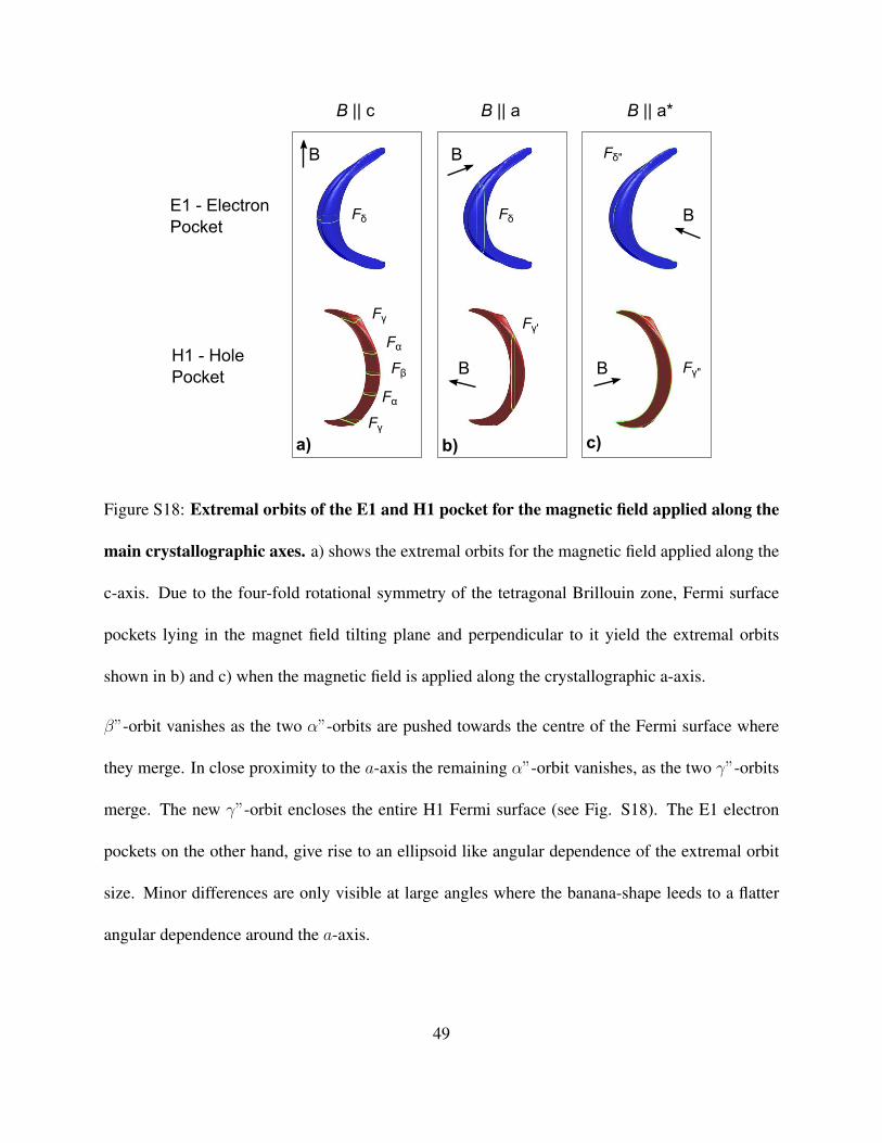
a) b) c)

Figure S18: Extremal orbits of the E1 and H1 pocket for the magnetic field applied along the

main crystallographic axes. a) shows the extremal orbits for the magnetic field applied along the

c-axis. Due to the four-fold rotational symmetry of the tetragonal Brillouin zone, Fermi surface

pockets lying in the magnet field tilting plane and perpendicular to it yield the extremal orbits

shown in b) and c) when the magnetic field is applied along the crystallographic a-axis.

β”-orbit vanishes as the two α”-orbits are pushed towards the centre of the Fermi surface where

they merge. In close proximity to the a-axis the remaining α”-orbit vanishes, as the two γ”-orbits

merge. The new γ”-orbit encloses the entire H1 Fermi surface (see Fig. S18). The E1 electron

pockets on the other hand, give rise to an ellipsoid like angular dependence of the extremal orbit

size. Minor differences are only visible at large angles where the banana-shape leeds to a flatter

angular dependence around the a-axis.

49

0

200

400

600

800

1000

1200

1400

k (arb. units)

A(k

)×h

/4π

e(T

)0

o

15o

30o

45o

60o

750

90o

0

200

400

600

800

1000

1200

1400

1600

k (arb. units)

A(k)×h/4

πe

(T)

0o

15o

30o

45o

60o

75o

90o

Figure S19: Angular dependence of the Fermi surface cross sections for B ∈ (100). The left

and right-hand side graphs show the k||B dependence of the Fermi surface cross section of the hole

(H) and electron (E) pocket for different magnetic field directions in the (100)-plane. Magnetic

field angles are measured relative to the c-axis. Extremal Fermi surface orbits are marked with

black dots and their respective names. Curves are shifted for clarity.

Compared to the band structure calculation we observe a more pronounced Fα neck-orbit. This

leads to a larger splitting of Fα and Fβ and increases the critical angle for the α and γ-orbit. Both

frequencies can observed up to B||a. The splitting of Fα and Fβ , i.e. their frequency difference

varies slightly between different band structure models and is beyond the resolution of our band

structure calculations. Similarly the splitting observed in δ is not reproduced by the calculation.

Here fine structures like a central waist in the electron pocket might give rise to the observed

splitting.

50

8 Quantum Limit

Due to the small bandwidth and low charge carrier effective mass in semi-metals like TaP, it is

comparably easy to tune these system into their magnetic quantum limit by applying moderate

magnetic fields13, 14. In the quantum limit the cyclotron energy ~ωc, i.e. the Landau level spacing,

exceeds the bandwidth of the Fermi surface pocket. The bandwidth of the electron and hole pocket

have been determined from our band structure calculation as ε ≈ 40 meV. Using the theoretical

effective masses (Tab. 1), we obtain quantum limit fields of 62 and 23 T for the electron and hole

pocket respectively. Using the experimental values, however, we obtain slightly lower fields of 51

and 17 T. Given both results, we can conclude, that none of the Fermi surface pockets goes to its

magnetic quantum limit in the magnetic field range studied in this letter.

9 Berry Phase

A central interest in Weyl semi-metals with broken inversion symmetry is the determination of

their Berry curvature or Berry phase ΦB by means of quantum oscillations15, 16.

In general the total quantum oscillation phase φ at 1/B = 0 can be extracted from the back

extrapolation of the Landau level index plotted against 1/B to zero. The total phase, which can be

extracted this way is the sum of three phase factors8, 17:

φ = 2π(γ + δ + ΦB), (5)

51

−1 −0.5 0 0.5 10

10

20

30

40

50

60

kz/πc

0

A(k

z)×h/

4π2 e

(T)

ElectronHole

Fγ Fγ

FβFαFα

Fδ

0 10 20 30 40 50 600

0.5

1

1.5

2

2.5

3x 105

F (T)

∆M(F

) (a

rb. u

nits

)

0 1 2−500

0

500

1/B (T−1)

∆M

Fα

Fβ

Fγ

Fδ

B||c

Figure S20: Simulated de Haas-van Alphen signal. The upper graph shows the kz dependence

of the Fermi surface cross-section of the electron and hole pocket for B||c. Here the extremal

cross-sections are marked with the name of their respective quantum oscillation frequencies. The

lower graph shows Fourier transform of the de Haas-van Alphen signal of the electron and hole

pocket as determined by Eqn. 6. The inset shows the raw dHvA signal.

52

where γ arises from the Onsager-Lifshitz quantisation and is ±1/2 for massive and 0 for

massless Fermions9. The phase factor δ depends on the Fermi surface curvature, i.e. d2Aext/dk2B

and can take values between +1/8 and −1/8. It is zero for two-dimensional Fermi surfaces where

d2Aext/dk2B = 0. Thus, it is generally not possible to determine the Berry phase ΦB without a

precise knowledge of the Fermi surface topology18–20.

In order to exclude the influence of δ in the determination of ΦB, we have simulated the dHvA-

signal for the electron and hole pocket (see Fig. S20). Here the oscillatory dHvA-magnetization

for magnetic field applied along the c-axis is defined as:

M ∝∫ π/c0

−π/c0sin

(~e

A(kz)

B

)dkz, (6)

where the A(kz) (Fig. S20) have been calculated from our band structure using the Fermi energy

of εF = 8.260 eV.

In Figure S21 the Landau level indices of the measured and simulated dHvA-oscillations for B||c

are plotted as function of the inverse magnetic field. Here the Landau level was assigned to the

falling zero-crossing of the oscillatory magnetization when plotted as a function of 1/B. Both

data are in excellent agreement and extrapolate to a φ/2π = 0.50 ± 0.03. We conclude that

γ+δ+φB = −0.5, which is indicative of a quasi-two dimensional orbit of massive charge carriers

with γ = −1/2 and δ = 0. This is also evidenced by the 1/ cos(θ)-like angular dependence of the

corresponding Fβ orbit. Furthermore, using Eqn. 5, we can exclude additional phases, such as the

Berry phase φB, as the measured total phase is in quantitative agreement with our semi-classical

model. Due to the negligible dHvA amplitudes of the other Fermi surface orbits it was not possible

53

0 0.25 0.5 0.75 1.0 1.25 1.50

5

10

15

20

25

1/B (T−1)

LL In

dex

exp. dataexp. fitsim. datasim. fit

Figure S21: Berry Phase plot forB||c. The graph shows the Landau level indices of experimental

and simulated de Haas-van Alphen oscillations as a function of the inverse magnetic field. Both

curves extrapolate to φ/2π = −0.50±0.03 at infinite field. The slope of both curves represents the

dominant Fβ orbit and is 17.55 and 17.80 T for the experimental and theoretical data respectively.

to determine their phase.

10 Scattering Times and Mobilities

The scattering time τ , mean free path l and charge carrier mobility µ can be determined from the

magnetic field dependence of the quantum oscillation amplitude i.e. the Dingle reduction term8, 21:

M(B) ∝ B−1/2 exp

(−14.69×m∗TD

B

). (7)

Here TD = ~/2πkBτ is the Dingle temperature, which is inversely proportional to the scattering

times. In reciprocal field and corrected for the√B-prefactor, the Dingle term represents an ex-

54

ponentially decaying envelope function, which results in a Lorentzian line shape observed in the

quantum oscillation spectra. As the full-width half-maximum of these Lorentzians lines ∆F1/2 is

directly related to the Dingle temperature by TD = ∆F1/2/(14.694πm∗), the line width can be used

to determine the Dingle temperature and scattering times in systems with complex dHvA-spectra.

The Dingle temperature of the hole pocket has been extracted from the Lorentzian line width. By

varying the magnetic field window, over which the data is Fourier transformed, at low fields, we

confirmed that the observed linewidths show no significant sinc-function contribution originating

from a finite window size. Here, the lowest magnetic field was chosen such that the quantum

oscillation amplitude has decayed to beneath the noise level. A double Lorentzian fit was applied

to the Fα -Fβ double peak to extract the linewidth of both signals. Simulations showed that for the

given window size and decay constants the sinc-contribution accounts for 1 and 21% of the total

linewidths of Fα and Fβ respectively. Based on the intrinsic linewidths, Dingle temperatures of

1.5±0.3K and scattering times of (8±2)×10−13s were calculated for both orbits. Using the fitted

effective masses we can calculate the charge carrier mean free path and mobility µ = τe/m∗ of

the hole charge carriers. We find that the hole mobility is µh ≈ (3.2± 0.5)× 104 cm2/Vs. Taking

into account the measured dHvA-frequencies, effective masses and assuming a parabolic band, the

mean free path of the holes can be calculated by applying: l = vF × τ with vF =√

2e~m∗2

F . Here,

we find a mean free path of lh = 0.4 µm. Performing the same analysis on the electron pocket was

not possible due to its comparably small signal size.

1. Uher, C. and Sander, L. Phys. Rev. B 27(2), 1326–1332 (1983).

55

2. Reed, W., Blount, E., Marcus, J., and Arko, A. J. Appl. Phys. 42(5453) (1971).

3. Yoshida, K. J. Phys. Soc. Jpn. 40(4) (1976).

4. Ueda, Y. and Kino, T. J. Phys. Soc. Jpn. 48(5) (1980).

5. Pippard, A. Magnetoresistance in Metals. Cambridge University Press, (1989).

6. Yoshida, K. J. Appl. Phys. 51(4226) (1980).

7. Singleton, J. Band Theory and Electronic Properties of Solids. Oxford Master Series in

Physics, (2001).

8. Shoenberg, D. Magnetic Oscillations in Metals. Cambridge University Press, (2009).

9. Onsager, L. Phil. Mag. 43(344), 1006–1008 (1952).

10. Lifshitz, I. and Kosevich, A. Sov. Phys. JETP 2, 636 (1956).

11. Lifshitz, I. and Kosevich, A. J. Phys. Chem. Solids. 4, 1–10 (1958).

12. Yamaji, K. J. Phys. Soc. Jpn. 58, 1520 (1989).

13. Yang, H., Fauque, B., Malone, L., Antunes, A., Zhu, Z., Uher, C., and Behnia, K. Nat. Comms.

47(1) (2010).

14. Arnold, F., Isidori, A., Kampert, E., Yager, B., Eschrig, M., and Saunders, J. ArXiv cond-

mat:str-el, 1411.3323v1 (2014).

15. He, L., Hong, X., Dong, J., Pan, J., Zhang, Z., Zhang, J., and Li, S. Rhys. Rev. Lett.

113(246402) (2014).

56

16. Weng, H., Fang, C., Fang, Z., Bernevig, B., and Dai, X. Phys. Rev. X 5(011029) (2015).

17. Hubbard, S., Kershaw, T., Usher, A., Savchenko, A., and Shytov, A. Phys. Rev. B 83(035122)

(2011).

18. Wang, Z., Zheng, Y., Shen, Z., Zhou, Y., Yang, X., Li, Y., Feng, C., and Xu, Z.-A. ArXiv

cond-mat:str-el, 1506.00924 (2015).

19. Luo, Y., Ghimire, N., Wartenbe, M., Neupane, M., McDonald, R., Thompson, E. B. J., and

Ronning, F. ArXiv cond-mat:str-el, 1506.01751v1 (2015).

20. Yang, X., Li, Y., Wang, Z., Zhen, Y., and Xu, Z. ArXiv cond-mat:str-el, 1506.02283v1 (2015).

21. Dingle, R. Proc. Roy. Soc. A 211(1107), 517–525 (1952).

57