Need for a Reference Frame1. Positions and velocities from geodetic

measurements:– Are not direct observations, but

estimated quantities– Are not absolute quantities– Need for a “Terrestrial Reference” in

which (or relative to which) positionsand velocities can be expressed.

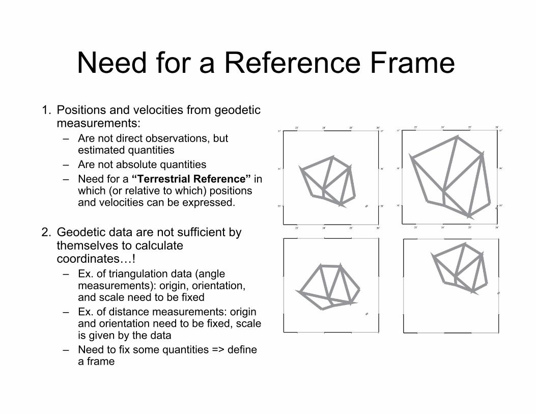
2. Geodetic data are not sufficient bythemselves to calculatecoordinates…!

– Ex. of triangulation data (anglemeasurements): origin, orientation,and scale need to be fixed

– Ex. of distance measurements: originand orientation need to be fixed, scaleis given by the data

– Need to fix some quantities => definea frame

Mathematically: the DatumDefect problem

• Assume measurements at 3 sites (in 3D):– 6 data:

• 2 independent distance measurements• 2 independent angle measurements• 2 independent height difference measurements

– 9 unknowns: [X,Y,Z] (or lat, lon, elev) at each site• For 4 sites: 12 unknowns, 9 data⇒ Datum defect = rank deficiency of the matrix that relates

the observations to the unknowns⇒ Solution: define a frame!

– Fix or constrain a number of coordinates– Minimum 3 coordinates at 2 sites to determine scale, orientation,

origin– A! a priori variance of site positions will impact the final

uncertainties (e.g., over-constraining typically results in artificiallysmall uncertainties)

System vs. Frame

• Terrestrial Reference System (TRS):– Mathematical definition of the reference in which

positions and velocities will be expressed.– Therefore invariable but “inaccessible” to users in

practice.• Terrestrial Reference Frame (TRF):

– Physical materialization of the reference systemby way of geodetic sites.

– Therefore accessible but perfectible.

The ideal TRS

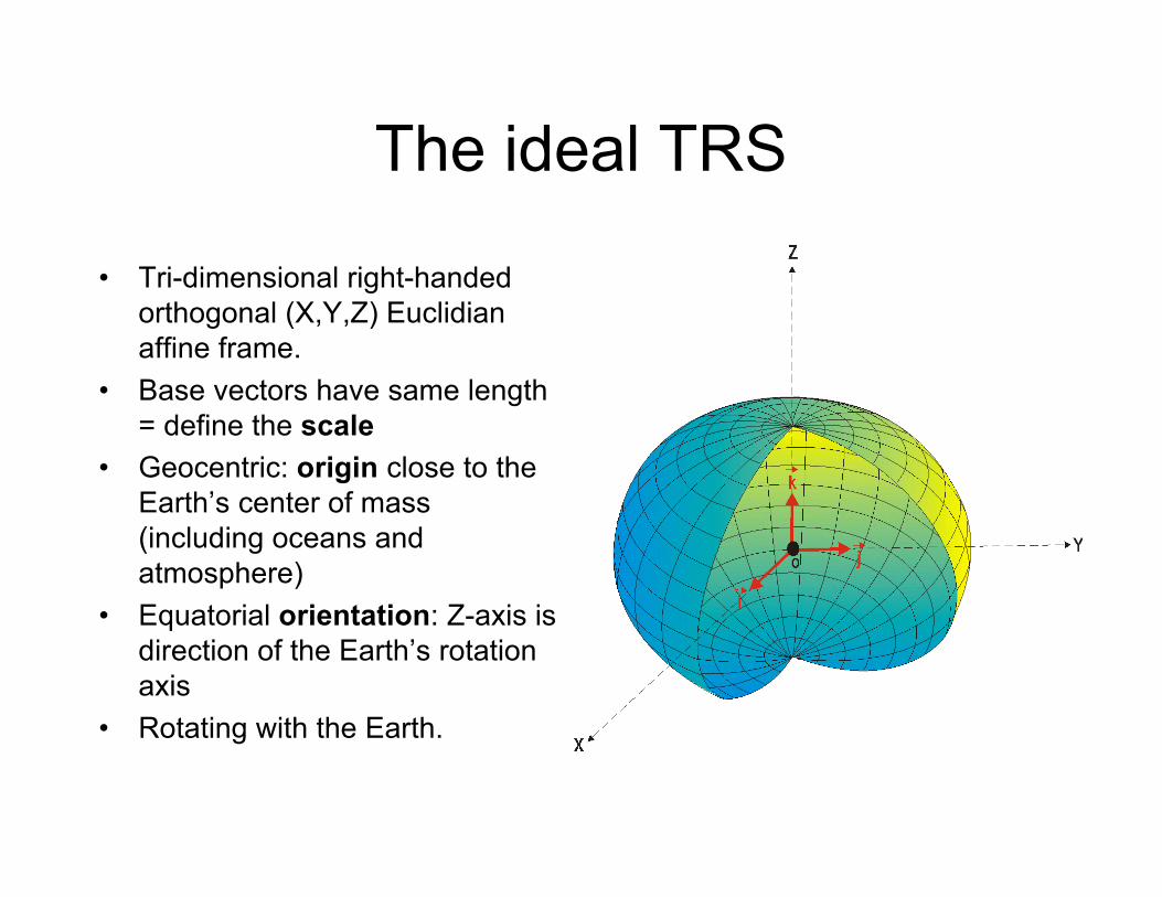
• Tri-dimensional right-handedorthogonal (X,Y,Z) Euclidianaffine frame.

• Base vectors have same length= define the scale

• Geocentric: origin close to theEarth’s center of mass(including oceans andatmosphere)

• Equatorial orientation: Z-axis isdirection of the Earth’s rotationaxis

• Rotating with the Earth.

3D similarity• Under these conditions, the

transformation of Cartesian coordinatesof any point between 2 TRSs (1) and (2)is given by a 3D similarity:

• Also called a Helmert, or 7-parameter,transformation:

– If translation (3 parameters), scale (1parameter) and rotation (3 parameters)are known, then one can convertbetween TRSs

– If there are common points between 2TRSs, one can solve for T, λ, R:minimum of 3 points.

!

X(2)

= T1,2

+ "1,2R1,2X(1)

X(1) and X(2) = position vectors in TRS(1) and TRS(2)T1,2 = translation vectorλ1,2 = scale factorR1,2 = rotation matrix

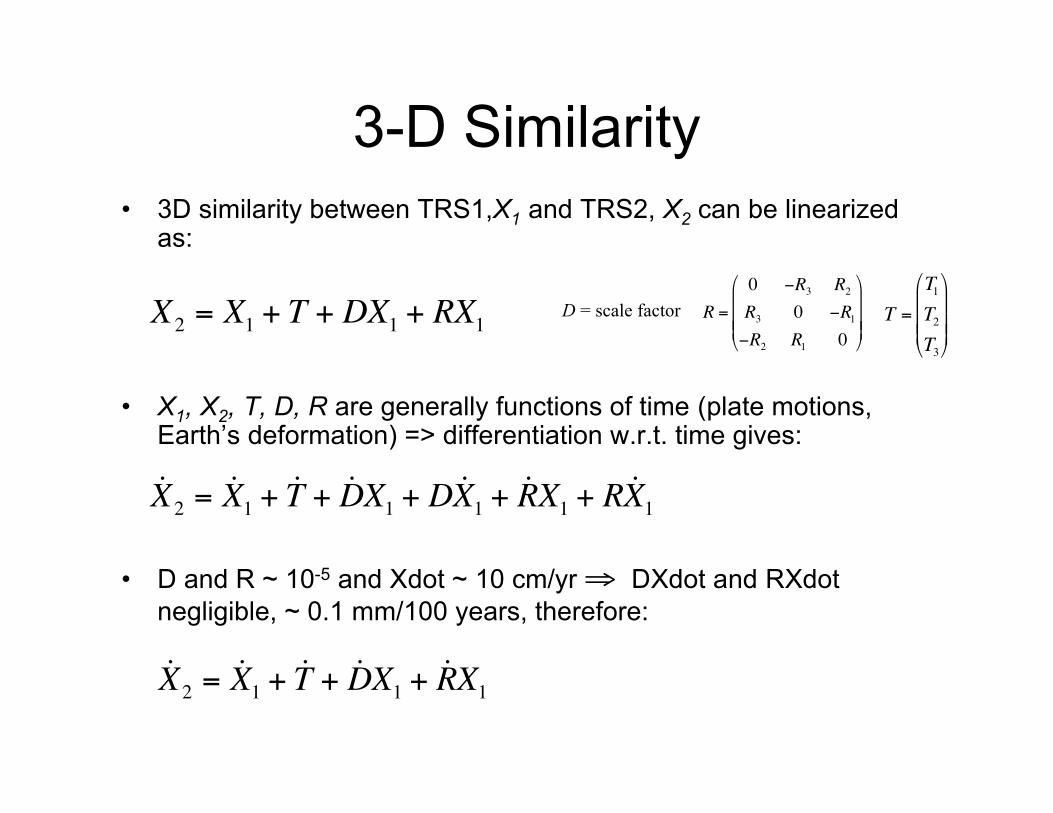
3-D Similarity• 3D similarity between TRS1,X1 and TRS2, X2 can be linearized

as:

• X1, X2, T, D, R are generally functions of time (plate motions,Earth’s deformation) => differentiation w.r.t. time gives:

• D and R ~ 10-5 and Xdot ~ 10 cm/yr ⇒ DXdot and RXdotnegligible, ~ 0.1 mm/100 years, therefore:

!

X2

= X1

+ T + DX1

+ RX1

!

T =

T1

T2

T3

"

#

$ $ $

%

&

' ' '

!

R =

0 "R3

R2

R3

0 "R1

"R2

R1

0

#

$

% % %

&

'

( ( (

D = scale factor

!

˙ X 2

= ˙ X 1+ ˙ T + ˙ D X

1+ D ˙ X

1+ ˙ R X

1+ R ˙ X

1

!

˙ X 2

= ˙ X 1+ ˙ T + ˙ D X

1+ ˙ R X

1

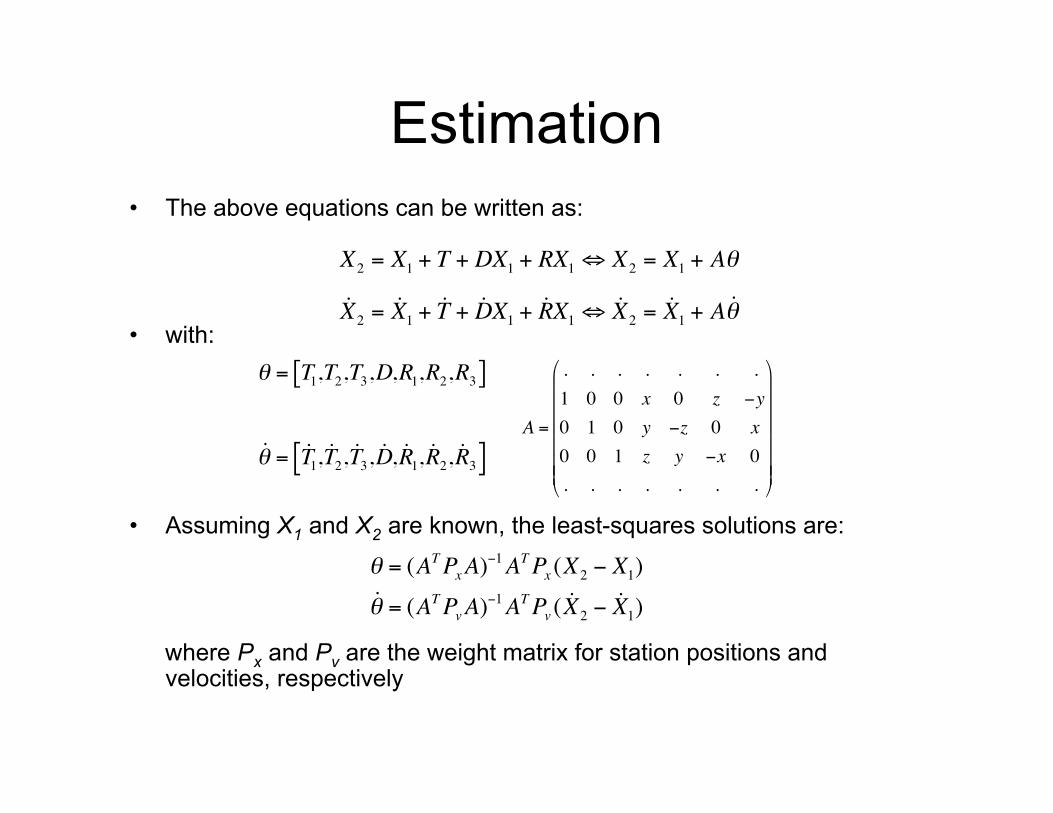
Estimation• The above equations can be written as:

• with:

• Assuming X1 and X2 are known, the least-squares solutions are:

where Px and Pv are the weight matrix for station positions andvelocities, respectively

!

˙ X 2

= ˙ X 1

+ ˙ T + ˙ D X1

+ ˙ R X1" ˙ X

2= ˙ X

1+ A ˙ #

!

X2

= X1

+ T + DX1

+ RX1" X

2= X

1+ A#

!

˙ " = ˙ T 1, ˙ T

2, ˙ T

3, ˙ D , ˙ R

1, ˙ R

2, ˙ R

3[ ]!

" = T1,T2,T3,D,R

1,R

2,R

3[ ]

!

A =

. . . . . . .

1 0 0 x 0 z "y

0 1 0 y "z 0 x

0 0 1 z y "x 0

. . . . . . .

#

$

% % % % % %

&

'

( ( ( ( ( (

!

" = (ATP

xA)

#1A

TP

x(X

2# X

1)

˙ " = (ATP

vA)

#1A

TP

v( ˙ X

2# ˙ X

1)

Problem when defining a frame…

• Unknowns = positions in frame 2 + 7 Helmertparameters => more unknowns than data = datumdefect

• Not enough data from space geodetic observations toestimate all frame parameters

• Solution: additional information– Tight constraints: estimated station positions/velocities are

constrained to a priori values within 10-5 m and a few mm/yr.– Loose constraints: same, with 1 m for position and 10 cm/yr

for velocities.– Minimal constraints.

Mathematically…

• The estimation of the coordinates of a network of GPS sites isoften done by solving for the linear system:

A = linearized model design matrix (partial derivatives) between the GPSobservations Obs and the parameters to estimate X. Σ-1

Obs is the weight matrixassociated to Obs (inverse of its covariance matrix).

• Solution is:

• But normal matrix N = ATΣObsA usually rank-defficient and notinvertible.

• To make the system invertible, one usually add constraints to theproblem by adding a condition equation to the normal equations.

!

AX =Obs "Obs

#1( )

!

X = (AT"Obs

#1A)

#1ATObs

Constraint equation• To make N invertible, one usually add constraints by using a condition

equation.• E.g., forcing the coordinates of a subset of sites to tightly follow values

of a given reference frame:

(Σa priori defines the constraint level, e.g. 1 cm in NE and 5 cm in U)• The resulting equation system becomes:

• And the solution:

!

Xcons = Xo "apriori

#1( )

!

A

I

"

# $ %

& ' Xcons =

Obs

Xo

"

# $

%

& '

(obs

)10

0 (apriori

)1

"

# $

%

& '

!

Xcons = AT"Obs#1A + "apriori

#1( )#1

AT"Obs#1Obs+ "apriori

#1( )Xo

Constrained solution• The covariance matrix of the constrained solution is given by:

• This can cause artificial deformations of the network if theconstraint level is too tight, given the actual accuracy of X0 =>errors propagate to the whole network.

• Also, the equation above modifies the variance of the result (andits structure). E.g., if constraint level very tight, the variance ofestimated parameters becomes artificially small.

• To avoid these problems, constraints have to be removed fromindividual solutions before they can be combined: suboptimal

• Better solution = minimal constraints.

!

"cons

#1= A

T"Obs#1A + "apriori

#1= "unc

#1+ "apriori

#1

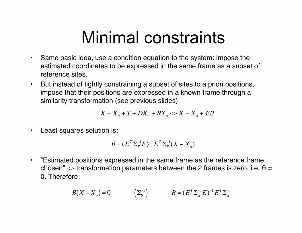
Minimal constraints• Same basic idea, use a condition equation to the system: impose the

estimated coordinates to be expressed in the same frame as a subset ofreference sites.

• But instead of tightly constraining a subset of sites to a priori positions,impose that their positions are expressed in a known frame through asimilarity transformation (see previous slides):

• Least squares solution is:

• “Estimated positions expressed in the same frame as the reference framechosen” ⇔ transformation parameters between the 2 frames is zero, i.e. θ =0. Therefore:

!

X = Xo

+ T + DXo

+ RXo" X = X

o+ E#

!

" = (ET#X

$1E)

$1ET#X

$1(X $ X

o)

!

B X " Xo( ) = 0 #$

"1( ) B = (ET#X

"1E)

"1ET#X

"1

Minimal constraints• Resulting equation system (with the condition equation) becomes:

• Solution is:

• With covariance:

• Covariance: reflects data noise + reference frame effect (via B)• Minimal constraints = algebraic expression on the covariance matrix

that the reference frame implementation is performed through asimilarity transformation.

!

A

B

"

# $ %

& ' Xmc

=Obs

BXo

"

# $

%

& '

(obs

)10

0 (*)1

"

# $

%

& '

!

Xmc

= AT"Obs

#1A + BT

"$#1B( )

#1

AT"Obs

#1Obs+ BT

"$#1B( )Xo

!

"mc

#1= A

T"Obs

#1A + B

T"$#1B = "

unc

#1+ B

T"$#1B

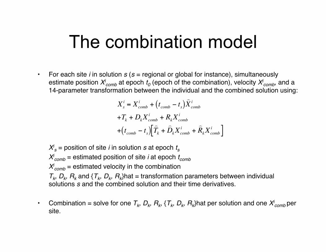
The combination model• For each site i in solution s (s = regional or global for instance), simultaneously

estimate position Xicomb at epoch t0 (epoch of the combination), velocity Xi

comb, and a14-parameter transformation between the individual and the combined solution using:

Xis = position of site i in solution s at epoch ts

Xicomb = estimated position of site i at epoch tcomb

Xicomb = estimated velocity in the combination

Tk, Dk, Rk and {Tk, Dk, Rk}hat = transformation parameters between individualsolutions s and the combined solution and their time derivatives.

• Combination = solve for one Tk, Dk, Rk, {Tk, Dk, Rk}hat per solution and one Xicomb per

site.

!

Xs

i = Xcomb

i + tcomb

" ts( )

) X

comb

i

+Tk

+ DkX

comb

i + RkX

comb

i

+ tcomb

" ts( )

) T

k+

) D

kX

comb

i +) R

kX

comb

i[ ]

In practice• Constrained solution can be done in globk (or glred) by tightly constraining

some sites (+ orbits) to a priori positions: ok for small networks (= localsolution)

• Minimally constrained solution computed in a 2-step manner:– Combine regional + global solutions in globk:

• Globk reads each solution sequentially and combines it to the previous one• Loose constraints applied to all estimated parameters• Chi2 change should be small is data consistent with model from previous slide• Output = loosely constrained solution

– Compute minimally constrained solution in glorg:• Matrix A comes from globk• Minimal constraints matrix B formed using sites that define frame

• Choice of reference sites:– Global distribution– Position and velocity precise and accurate– Error on their position/velocity and correlations well known