nearby cycles of parahoric shtukas, and a fundamental...
TRANSCRIPT

NEARBY CYCLES OF PARAHORIC SHTUKAS,AND A FUNDAMENTAL LEMMA FOR BASE CHANGE
TONY FENG
Abstract. Following the paradigm initiated by Kottwitz, we compute the trace of Frobenius composedwith Hecke operators on the cohomology of nearby cycles, at places of parahoric reduction, of perversesheaves on certain moduli stacks of shtukas. Inspired by an argument of Ngô, we then use this to givea geometric proof of a base change fundamental lemma for parahoric Hecke algebras for GLn over localfunction fields. This generalizes a theorem of Ngô, who proved the base change fundamental lemma forspherical Hecke algebras for GLn over local function fields, and extends to positive characteristic (for GLn)a fundamental lemma originally introduced and proved by Haines for p-adic local fields.
Contents
1. Introduction 12. Statement of results and overview of the paper 43. Notation 84. Moduli of shtukas 95. The Kottwitz Conjecture for shtukas 166. Counting parahoric shtukas 207. Geometrization of base change for Hecke algebras 258. Comparison of two moduli problems 329. Calculation of traces on the cohomology of nearby cycles 34References 39
1. Introduction
There are two main goals of this paper:(1) To compute the trace of Frobenius composed with Hecke operators on the cohomology of nearby
cycles at places of parahoric reduction for certain moduli stacks of shtukas, and(2) To parlay the resulting formulas into a geometric proof of a fundamental lemma for base change for
central elements in parahoric Hecke algebras over local function fields.The first goal is accomplished by using the Grothendieck-Lefschetz trace formula to break up the computationof the trace into two pieces: (1) counting points on certain moduli spaces, and (2) understanding the stalksof the nearby cycles sheaves. These pieces are then each resolved by a sequence of technical steps whoseoverall strategy is rather well-known, and which would require a considerable amount of notation to describe.Therefore, in this introduction we will focus on informally explaining the idea of the second goal.
The fundamental lemma of interest was proposed and proved by Haines [Hai09] for p-adic (i.e. mixedcharacteristic) local fields, and generalizes the fundamental lemma for base change for spherical Hecke alge-bras proved (independently) in the p-adic case by Clozel [Clo90] and Labesse [Lab90], building on work ofKottwitz [Kot86a], and in the function field case (for GLn) by Ngô [Ngo06].
The original motivation for this fundamental lemma was to study the cohomology of a Shimura variety withparahoric level structure, and in particular to determine the semisimple zeta factor at a place of parahoricreduction. The fundamental lemma enters in comparing the trace of Frobenius and Hecke operators on thiscohomology with the geometric side of the Arthur-Selberg trace formula. We refer the interested reader to[Hai09], especially p. 573, for more details.
1

2 TONY FENG
The same applications are available in the function field setting, with Shimura varieties replaced by themoduli stacks of shtukas, which have been utilized by Drinfeld ([Dri87], for GL2), L. Lafforgue ([Laf02], forGLn), and V. Lafforgue ([Laf12], for general reductive groups) to spectacular success towards the globalLanglands correspondence over function fields.
However, in this paper we have chosen to emphasize the geometric aspect of the fundamental lemma,rather than its applications to the Langlands program. In contrast to the proof of [Hai09] for p-adic case,which following in the tradition of [Clo90] and [Lab90] is via p-adic harmonic analysis, our proof works byexploiting additional geometry and structure which is available in the function field setting. Our strategy isvery much based on that of [Ngo06], and indeed specializes to it in the case of spherical Hecke algebras. Wethink it would be useful to give an impressionistic preview of the strategy now. A more detailed overviewwill be given in §2.1 and §2.2.
Broadly speaking, the base change fundamental lemma compares an orbital integral with a twisted orbitalintegral. To elaborate, let F be a local field, G a reductive group over F , γ ∈ G(F ), and f a function onG(F ). The orbital integral corresponding to this data is
Oγ(f) :=
∫G(F )/Gγ(F )
f(g−1γg) dg (1.1)
where Gγ(F ) is the centralizer of γ in G(F ). We will take f to be in an appropriate Hecke algebra HG(F ).(Of course we also need to discuss the normalization of Haar measures, but let us leave that for §2.1.)
Let E/F be an unramified extension of degree r, δ ∈ G(E), and fE a function on G(E). The twistedorbital integral corresponding to this data is
TOδσ(fE) :=
∫G(E)/Gδσ(F )
fE(g−1δσ(g)) dg (1.2)
where σ ∈ Gal(E/F ) is the lift of (arithmetic) Frobenius, and
Gδσ(F ) := {g ∈ G(E) : g−1δσ(g) = δ}
is the twisted centralizer of γ in Gδσ(E). Again, we will take fE to be in an appropriate Hecke algebraHG(E).
If HG(E),J and HG(F ),J are corresponding parahoric Hecke algebras, then there is a base change homo-morphism for their centers
b : Z(HG(E),J)→ Z(HG(F ),J).
There is also a norm map N from stable twisted conjugacy classes in G(E) to stable conjugacy classes inG(F ).
In the special case G = GLn, the base change fundamental lemma for the center of parahoric Heckealgebras predicts that for σ-regular, σ-semisimple δ ∈ G(E) and fE ∈ Z(HG(E),J), we have
TOδσ(fE) = ON(δ)(b(fE)). (1.3)
This is almost what we will prove. (For more general G, the formulation is more complicated; see [Hai09],Theorem 1.0.3 and §5.)
Now we can describe our strategy of proof of (1.3). The starting point is the seminal work of Kottwitz oncounting points of Shimura varieties over finite fields. In [Kot92] Kottwitz proves a formula expressing thetrace of Frobenius composed with a Hecke operator on the cohomology of certain PEL Shimura varieties asa sum of a product of (twisted) orbital integrals:
Tr(h ◦ Frobp, H∗(ShK ,Q`)) =
∑(. . .)Oγ(hp)TOδσ(hp) (1.4)
where ShK is an appropriate Shimura variety and h is a Hecke operator. In fact the purpose of the funda-mental lemma is to re-express the twisted orbital integrals in (1.4), so as to be able to compare the expressionwith the geometric side of the Arthur-Selberg trace formula. But in this paper we adopt an opposite per-spective, instead viewing (1.4) as giving a geometric interpretation of (twisted) orbital integrals (in the p-adiccase) in terms of the cohomology of Shimura varieties.
In the function field setting, which is the one of interest to this paper, one can prove an analogous formulaof the form
Tr(hA ◦ Frobx0 ◦τ,H∗(ShtA,A)) =∑
(. . .)Oγ(hx0
A )TOδσ(hA,x0) (1.5)

NEARBY CYCLES OF PARAHORIC SHTUKAS, AND A FUNDAMENTAL LEMMA FOR BASE CHANGE 3
for an appropriate moduli stack ShtA, an appropriate sheaf A, an appropriate Hecke operator hA, and anadditional symmetry τ . (Roughly, τ is a “rotation” symmetry that arises from the moduli problem.)
However, it turns out that we can also construct a moduli stack ShtB such that
Tr(hB ◦ Frobx0◦τ,H∗(ShtB ,B)) =
∑(. . .)Oγ(hx0
B )Oδσ(b(hB,x0)) (1.6)
for an appropriate sheaf B, an appropriate Hecke operator hB , and an additional symmetry τ similar to thatfrom (1.5). The crucial point is that in (1.6) the twisted orbital integral is replaced with the orbital integralof a base changed function.
We remark that the computations (1.5) and (1.6) were obtained in [Ngo06] for places of good (hyperspecial)reduction, in which case one finds a spherical Hecke operator. In the present work, which concerns placesof parahoric bad reduction, the analogous computations (1.5) and (1.6) are of independent interest, andactually form the main content of this paper. They require several nontrivial inputs, including, for theparahoric setting that we study here, a version of the Kottwitz Conjecture for shtukas, as well as a geometricinterpretation of the base change homomorphism for Hecke algebras. Nevertheless, let us elide these pointsfor now.
The upshot is that (1.5) and (1.6) translate the problem of comparing orbital integrals and twisted orbitalintegrals into comparing (the cohomology of) two different moduli problems ShtA and ShtB . (We remarkthat the relationship we seek turns out to be subtler than equality, but again we elide this issue for now.)
At this point the particular the choice of ShtA and ShtB becomes crucial. Therefore, to proceed with thediscussion we will need to give some idea of what these moduli problems look like. In (1.4) the Shimuravariety ShK is defined over an open subset of the ring of integers of a number field, whereas in (1.5) and(1.6) the moduli stacks ShtA and ShtB are defined over an open subset X◦ of a curve over a finite field Fq.The moduli stack ShtA parametrizes “independent” modifications of vector bundles Ei over X◦, with themodifications occuring over the point x:
ShtA “ = ”
x ∈ X◦σE1
x99K E1
σE2x99K E2...
σErx99K Er
.
(Here the superscript σ refers to a Frobenius twist, which has not been explained but is a standard part ofthe definition of shtukas.) On the other hand, the moduli stack ShtB parametrizes “iterated” modificationsof G-bundles Ei over X◦:
ShtB “ = ”
{x ∈ X◦
σErx99K E1
x99K . . .
x99K Er
}.
Forgetting everything except x defines maps
ShtA ShtB
X◦ X◦
Now the key point is that we can deform these moduli problems by allowing the points of modification tovary over X◦ (which of course is a trick only available in the function field setting). More precisely, we canconstruct extended moduli stacks
ShtA ShtB
(X◦)r (X◦)r
πA πB
4 TONY FENG
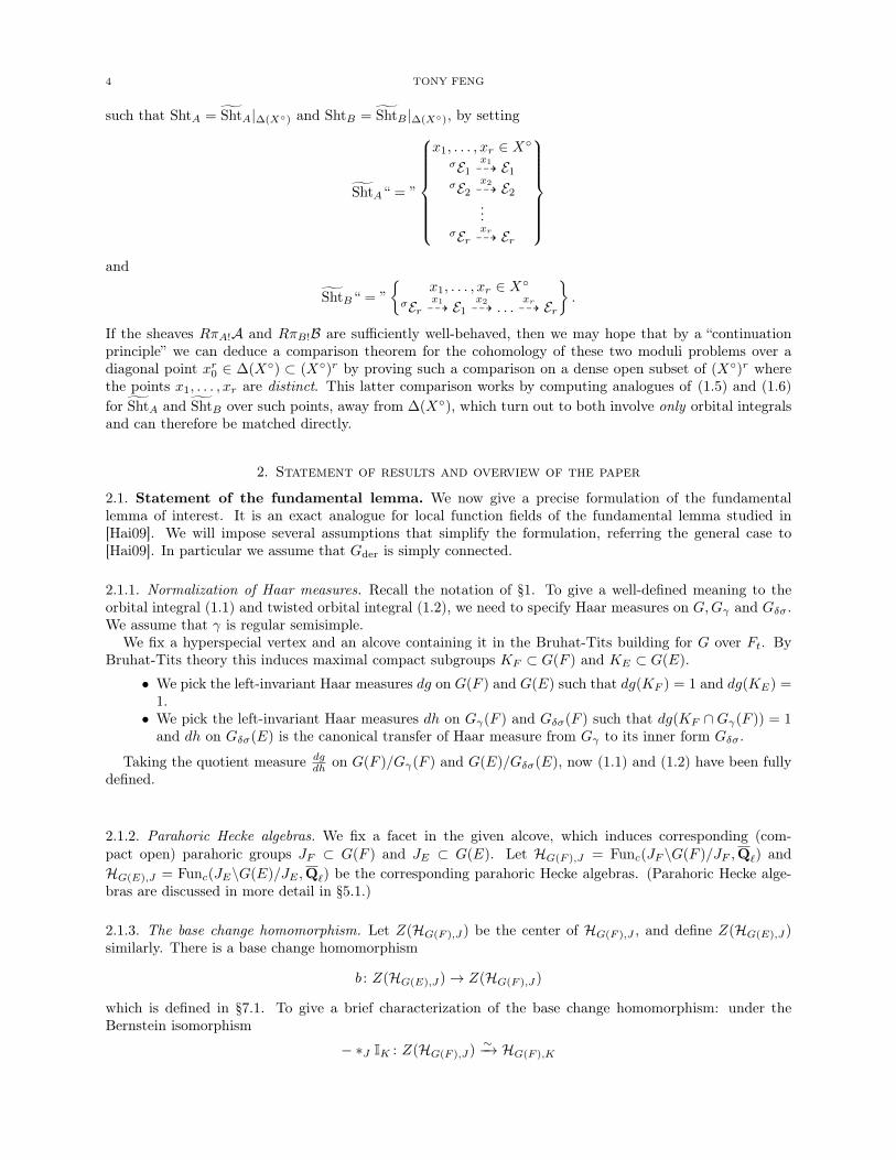
such that ShtA = ShtA|∆(X◦) and ShtB = ShtB |∆(X◦), by setting
ShtA“ = ”
x1, . . . , xr ∈ X◦σE1
x199K E1
σE2x299K E2...
σErxr99K Er
and
ShtB“ = ”
{x1, . . . , xr ∈ X◦
σErx199K E1
x299K . . .
xr99K Er
}.
If the sheaves RπA!A and RπB!B are sufficiently well-behaved, then we may hope that by a “continuationprinciple” we can deduce a comparison theorem for the cohomology of these two moduli problems over adiagonal point xr0 ∈ ∆(X◦) ⊂ (X◦)r by proving such a comparison on a dense open subset of (X◦)r wherethe points x1, . . . , xr are distinct. This latter comparison works by computing analogues of (1.5) and (1.6)for ShtA and ShtB over such points, away from ∆(X◦), which turn out to both involve only orbital integralsand can therefore be matched directly.
2. Statement of results and overview of the paper
2.1. Statement of the fundamental lemma. We now give a precise formulation of the fundamentallemma of interest. It is an exact analogue for local function fields of the fundamental lemma studied in[Hai09]. We will impose several assumptions that simplify the formulation, referring the general case to[Hai09]. In particular we assume that Gder is simply connected.
2.1.1. Normalization of Haar measures. Recall the notation of §1. To give a well-defined meaning to theorbital integral (1.1) and twisted orbital integral (1.2), we need to specify Haar measures on G,Gγ and Gδσ.We assume that γ is regular semisimple.
We fix a hyperspecial vertex and an alcove containing it in the Bruhat-Tits building for G over Ft. ByBruhat-Tits theory this induces maximal compact subgroups KF ⊂ G(F ) and KE ⊂ G(E).
• We pick the left-invariant Haar measures dg on G(F ) and G(E) such that dg(KF ) = 1 and dg(KE) =1.• We pick the left-invariant Haar measures dh on Gγ(F ) and Gδσ(F ) such that dg(KF ∩Gγ(F )) = 1
and dh on Gδσ(E) is the canonical transfer of Haar measure from Gγ to its inner form Gδσ.
Taking the quotient measure dgdh on G(F )/Gγ(F ) and G(E)/Gδσ(E), now (1.1) and (1.2) have been fully
defined.
2.1.2. Parahoric Hecke algebras. We fix a facet in the given alcove, which induces corresponding (com-pact open) parahoric groups JF ⊂ G(F ) and JE ⊂ G(E). Let HG(F ),J = Func(JF \G(F )/JF ,Q`) andHG(E),J = Func(JE\G(E)/JE ,Q`) be the corresponding parahoric Hecke algebras. (Parahoric Hecke alge-bras are discussed in more detail in §5.1.)
2.1.3. The base change homomorphism. Let Z(HG(F ),J) be the center of HG(F ),J , and define Z(HG(E),J)similarly. There is a base change homomorphism
b : Z(HG(E),J)→ Z(HG(F ),J)
which is defined in §7.1. To give a brief characterization of the base change homomorphism: under theBernstein isomorphism
− ∗J IK : Z(HG(F ),J)∼−→ HG(F ),K

NEARBY CYCLES OF PARAHORIC SHTUKAS, AND A FUNDAMENTAL LEMMA FOR BASE CHANGE 5
obtained by convolving with the indicator function IK , it corresponds to the usual base change homomor-phism for spherical Hecke algebras.
Z(HG(E),J) Z(HG(F ),J)
HG(E),K HG(F ),K
b
−∗J IK∼ −∗J IK∼
b
2.1.4. The norm map. Let σ ∈ Gal(E/F ) be a lift of (arithmetic) Frobenius. The “concrete norm”
NmE/F : G(E)→ G(F )
defined byNmE/F (δ) := δ · σ(δ) · . . . σr−1(δ)
descends to a norm map
N : G(E)/stable σ-conjugacy→ G(F )/stable conjugacy.
2.1.5. Formulation of the fundamental lemma. The following fundamental lemma was proved by Haines inthe p-adic setting ([Hai09], Theorem 1.0.3.)
Theorem 2.1 (Haines). Let E/F be an unramified extension of p-adic local fields of degree r and residuecharacteristic p. Let ψ ∈ Z(HG(E),J) and δ ∈ G(E) such that N(δ) is semisimple. Then we have
SOG(E)δσ (ψ) = SOG
N(δ)(b(ψ)).
Here SO are stable (twisted) orbital integrals, for whose definition we refer to [Hai09] §5.1. Since oureventual result will be for G = GLn, where stable conjugacy coincides with conjugacy, we can ignore theissue of stabilization.
Remark 2.2. Haines has informed us that his proof, which is based on the global simple trace formula andKottwitz’s stabilization of the twisted trace formula, does not carry over (at least, not without nontrivialadditional work) to the positive characteristic setting. 1
We now formulate our main result, which is an extension (in a special case) of Theorem 2.1 to positivecharacteristic.
By the Bernstein isomorphism, a basis for Z(HG(E),J) is given by the functions ψµ for µ a dominantcoweight of G, which correspond under −∗J IK to the indicator functions of the double coset inKE\G(E)/KE
indexed by µ.
Example/Definition 2.3. If G = GLn, and T ⊂ GLn is the usual (diagonal) maximal torus, then wemay identify X∗(T ) ∼= Zn in the standard way. The dominant weights coweights X∗(T )+ are those µ =(µ1, . . . , µn) with µ1 ≥ µ2 ≥ . . . ≥ µn. We define
|µ| := µ1 + . . .+ µn.
In this paper we prove:
Theorem 2.4. Let E/F be an unramified degree r extension of characteristic p local fields. If δ ∈ GLn(E)is such that N(δ) is regular semisimple and separable, and ψ ∈ Z(HGLn(E),J) is a linear combination of ψµwith |µ| = 0, then we have
TOδσ(ψ) = ON(δ)(b(ψ)).
Remark 2.5. Let us make some remarks on the hypotheses. The hypothesis |µ| = 0 arises geometrically asa condition for the non-emptiness of moduli stacks of shtukas.
The restriction to GLn comes from a need to obtain a proper moduli stack, in order to have enough controlover the cohomology of the relevant moduli stacks of shtukas. In general the moduli stacks of shtukas are ofinfinite type, and their cohomology not constructible. However, for GLn we can use the trick of globalizingto a division algebra in order to create a proper global space with the right local behavior.
1However, we note that W. Ray Dulany proved the base change fundamental lemma for GL2 by hand in the function fieldcase [RD]. We thank Tom Haines for informing us about Ray Dulany’s work.

6 TONY FENG
Remark 2.6. It seems likely that the theorem can be extended to prove Conjecture 2.1 in full for G = GLnusing methods that are by now considered “standard”, as in [Clo90]. One reason we have not bothered todo this is that the constraint |µ| = 0 is necessary in order to make the geometric objects non-trivial, and sois satisfied in applications of the fundamental lemma to study the cohomology of moduli stacks of shtukasvia the Arthur-Selberg trace formula. Therefore, Theorem 2.4 should be adequate for applications to theLanglands program.
Remark 2.7. As T. Haines pointed out to us, another key aspect of the fundamental lemma is the assertionthat Oγ(b(ψ)) = 0 if γ is not a norm. Our strategy does not seem to naturally give access to this statement.On the other hand, since Labesse gave a purely local proof of this statement for the spherical case in mixedcharacteristic, which was extended to the center of parahoric Hecke algebras in [Hai09] §5.2, it shouldgeneralize to positive characteristic. We intend to include this in a future work, when it becomes necessary.
2.1.6. Related work. The fundamental lemma for base change for spherical Hecke algebras, which arises fromTheorem 2.1 in the special case where J = K is a hyperspecial maximal compact subgroup, was proved inthe p-adic case by Clozel [Clo90] and Labesse [Lab90], using key input from Kottwitz [Kot86a] who checkedit for the unit element. These arguments were generalized by Haines to proved the base change fundamentallemma for centers of parahoric Hecke algebras, as has been discussed.2
For local function fields (i.e. positive characteristic), the spherical case J = K of Theorem 2.4 wasestablished by Ngô [Ngo06], also for GLn and also for |µ| = 0 (with the same reasons for the restrictions).Indeed, our strategy as described in §1 is the one pioneered by [Ngo06]. Similar results were obtainedindependently and simultaneously by Lau [Lau04]. The key to our generalization is that in the parahoriccase, we know enough about the nearby cycles sheaf at a place of bad reduction, thanks to the proof of a“Kottwitz Conjecture for shtukas” due to Gaitsgory [Gai01], to carry out the geometric argument.
2.2. Overview of the proof. Let us now give a more detailed overview of the proof of Theorem 2.4. Weare trying to prove a local result, but we will immediately shift to a global setting. Therefore, we changenotation from before. Let Fx0
be a local function field of characteristic p, so we have non-canonically
Fx0∼= Fq((t)).
As the notation suggests, we view Fx0as the completion of a global function field F at a place x0, and we
view F as the global function field of a smooth projective curve X/Fq. (Note that we have implicitly takenx0 to be a point of degree one on X, which is actually important.)
Let G be a reductive group over F and J ⊂ G(Fx0) a parahoric subgroup. We choose any extension ofG to parahoric group scheme G → X such that over the completed local ring Spec (Ox0
:= OX,x0), we have
G(Ox0) = J . We assume that G⊗F Fx is split at all x where G(Ox) is not hyperspecial.
Following [Ngo06], in §8 we define two moduli stacks of G-shtukas which we call ShtA and ShtB . (We haveincluded a background section summarizing the essential constructions and facts about shtukas in §4.) LetE/F be the unramified extension of degree r. As outlined in §1, the goal is threefold:
(1) Obtain an expression relating the trace of Frobenius composed with Hecke operators on the coho-mology of ShtA to the twisted orbital integral of ψ ∈ Z(HG(Ex0 ),J).
(2) Obtain an expression relating trace of Frobenius composed with Hecke operators on the cohomologyof ShtB to the orbital integral of the base changed function b(ψ).
(3) Relate the two cohomology groups in question in some other way.Let us discuss each of these tasks in turn. For (1), we need a geometric interpretation of the center of theparahoric Hecke algebra HG(Fx0
),J . It is well-known that the spherical Hecke algebra is geometrized, underthe function-sheaf dictionary, by perverse sheaves on the affine Grassmannian. Similarly, the parahoric Heckealgebra is geometrized by a partial affine flag variety.
This story is globalized by the Beilinson-Drinfeld Grassmanian GrG → X. Over a general point of Xthe fiber of GrG is an affine Grassmannian, but because G is a parahoric group at x0, the fiber over x0 isactually a partial affine flag variety. It is essentially a result of Gaitsgory, although the formulation in [Gai01]
2See the last paragraph of the introduction to [Hai09] for a discussion of to what extent Conjecture 2.1 follows from thefundamental lemma for twisted endoscopy. Although base change is a special case of twisted endoscopy, the fundamental lemmafor twisted endoscopy should imply that there is a matching function for ψ, but does not identify it in terms of the base changehomomorphism.

NEARBY CYCLES OF PARAHORIC SHTUKAS, AND A FUNDAMENTAL LEMMA FOR BASE CHANGE 7
is slightly different, that the nearby cycles functor takes perverse sheaves on GrG |X−x0 to central perversesheaves on GrG |x0
∼= FlG,J .Using this, in §5 we relate the trace function associated to the nearby cycles sheaf at x0 of perverse sheaves
on ShtG to central elements of HG,J . This is the desired geometrization of Z(HG(Ex0),J). The key point is
that the Beilinson-Drinfeld Grassmannian is a smooth (even étale) local model for ShtG .In §6 we give a counting formula for points of ShtA, in the style of Kottwitz [Kot92]. This formula is based
on [Ngo06] and [NND08]; however we must note that it only gives a “partial formula”, counting only thosepoints indexed by an elliptic Kottwitz triple. Indeed, since the moduli stacks of shtukas are of infinite typein general (even with full level structure and bounded modifications), they can have infinitely many pointsover finite fields in general, which makes it somewhat subtle to give a meaningful formula. This issue canbe bypassed altogether for GLn by taking G to be the group associated to a sufficiently ramified divisionalgebra over X, with G(Fx0
) ∼= GLn(Fx0). This trick is one major reason for the restriction to GLn; another
(which is morally of the same nature) will arise in the discussion of (3).These ingredients are put together in §9.1, obtaining a formula
Tr((hβ ⊗ 1 . . .⊗ 1) ◦ Frobx0 ◦τ,RΨxr0(Aµr )) =
∑(. . .)
∏v 6=x0
Oγv (fβv )
· TOδx0σ(ψ′r,µ). (2.1)
See Theorem 9.2 for the precise statement.
Now we turn our attention to (2). All the same ingredients and steps are required as in (1), but now weadditionally need a geometric interpretation of the base change homomorphism
b : Z(HG(Ex0),J)→ Z(HG(Fx0
),J).
This problem is studied in §7 for split reductive G, generalizing results of Ngô for GLn [Ngo99]. First,by a local study of the affine Grassmannian we prove the following fact. Let SatGrG(µ) be the perversesheaf on GrG corresponding, under Geometric Satake, to the dominant coweight µ ∈ X∗(T )+, and let ψr,µbe the trace function of Frobr on SatGrG(µ); thus ψr,µ ∈ HG,K(Ex0). Then b(ψr,µ) is the trace functionassociated to Frob ◦κ′ on SatGrG(µ)∗r, where SatGrG(µ)∗r is the r-fold convolution of SatGrG(µ) and κ′ isa cyclic permutation of order r using from the commutativity constraint on perverse sheaves on the affineGrassmannian [MV07]. See Theorem 7.15 for the precise statement. We emphasize again that this wasobtained already by Ngô for GLn, which is really the only situation where we can currently prove Conjecture2.1; we prove the more general statement here in anticipation of future generalizations.
Using the global degeneration from a Beilinson-Drinfeld Grassmanian, we prove an analogous generaliza-tion to the center of parahoric Hecke algebras in terms of nearby cycles sheaves; see Theorem 7.17 for theprecise statement. This result is used as a local model to understand sheaves on ShtB , and is assembled in§9.2 in conjunction with the ingredients mentioned in the discussion of (1) to obtain a formula
Tr(hβ ◦ Frobx0 ◦τ,RΨxr0(Bµr )) =
∑(. . .)
∏v 6=x0
Oγv (fβv )
·Oγx0(b(ψ′r,µ)). (2.2)
See Theorem 9.3 for the precise statement.
Finally, we address (3). As discussed in §1 the moduli problems ShtA and ShtB are actually defined over(X◦)r. By analogous but easier arguments we can prove that
Tr((hβ ⊗ 1 . . .⊗ 1) ◦ Frobx ◦τ,Aµr ) = Tr(hβ ◦ Frobx ◦τ,Bµr )
for x ∈ (X◦)r consisting of r pairwise-distinct points. (We caution that the relationship between Aµr and Bµris not one of equality. Rather, the former is more like the rth tensor power of the latter, and the equality oftraces is the nonobvious linear algebraic identity in Lemma 7.13.) In other words, we can obtain analoguesof (2.1) and (2.2) which are manifestly equal at sufficiently many (by Chebotarev density) x. In fact sinceShtA and ShtB have good (hyperspecial) reduction at almost all such x this already follows from [Ngo06] §5,where the proof is exactly as was just indicated; we give a more detailed sketch of Ngô’s proof in §8.4.
However, knowing the equality for x ∈ U := (X◦)r − ∆(X◦) is not itself sufficient for deducing anequality at a point of ∆(X◦). It would be sufficient if the sheaves Aµr and Bµr were local systems in a

8 TONY FENG
neighborhood of a point of ∆(X◦) ⊂ (X◦)r. In fact, since they are equipped with a partial Frobeniusstructure, by “Drinfeld’s Lemma” ([Dri87] Proposition 6.1, [Lau04] Lemma 9.2.1) if they were even merelyconstructible then they would automatically be local systems in a neighborhood of the generic point of∆(X◦) ⊂ (X◦)r. Unfortunately, as has already been discussed, the moduli stacks of shtukas are of infinitetype in general, and their cohomology is not even constructible on (X◦)r. Here again we invoke the trick ofusing a sufficiently ramified division algebra in order to enforce the properness of the global moduli stack,and thus the constructibility; of course the cost is that this only gives results for GLn.
2.3. Summary of the paper. Although we discussed in §2.2 why our current argument does not workbeyond GLn, we hope that after future technical improvements in the theory of shtukas it can be generalizedto a much wider class of reductive groups. For this reason, for the individual steps we have tried to workwith more general groups when possible. It seems worthwhile to give a brief outline of the organization ofthe paper, pointing out exactly where we can be more general.
In §4 we review the theory of shtukas for nonconstant reductive group schemes, summarizing the essentialbackground facts. Also, a key point is to define an “integral model” for the moduli stack of shtukas, extendingover points of parahoric bad reduction.
In §5 we establish an analogue of the Kottwitz Conjecture for moduli of shtukas. This works even forfairly general (not necessarily constant) reductive groups G → X: Gaitsgory originally proved it for constantgroups, and his argument was generalized by Zhu in [Zhu14] Theorem 7.3 and Pappas-Zhu in [PZ13].
In §6 we establish some counting formulas for points of shtukas over finite fields. This is a minor variantof the work of Ngô B.C. and Ngô Dac T., which was previously only formulated at places hyperspecial levelstructure. Our contribution is to write it out for the case of parahoric bad reduction that we require.
In §7 we provide a geometric interpretation of the base change homomorphism for spherical Hecke algebrasand the center of parahoric Hecke algebras for general split reductive groups G over a local field. For GLnthis was proved by Ngô, in a formulation that was rather specific to GLn. We generalize the argument tospherical Hecke algebras for arbitrary split reductive groups, and then use that to deduce a result for (centralelements in) parahoric Hecke algebras.
In §8 we introduce the two moduli problems ShtA and ShtB which are to be compared, and recall Ngô’stheorem stating the precise comparison. Using this we deduce an equality of traces on the nearby cyclessheaves at the point of parahoric reduction. Here we also crucially use that the moduli of shtukas associatedto a sufficiently ramified division algebra is proper, which implies that the cohomology is a local system.
In §9 we compute these traces in terms of (twisted) orbital integrals, giving formulas in the paradigm ofKottwitz, and then use them in §9.3 to deduce the cases of the base change fundamental lemma claimed inTheorem 2.4.
2.4. Acknowledgments. I am indebted to Zhiwei Yun for teaching me basically everything that I knowabout shtukas, and in particular for directing me to [Ngo06]. I would also like to thank Zhiwei, LaurentClozel, Gurbir Dhillon, Tom Haines, Jochen Heinloth, Urs Hartl, Bao Le Hung, and Rong Zhou for helpfulconversations related to this work. This document benefited enormously from comments, corrections, andsuggestions by Brian Conrad, Tom Haines, and Timo Richarz.
This project was conceived at the 2017 Arbeitsgemeinschaft in Oberwolfach, and completed while I wasa guest at the Institute for Advanced Study, and under the support of an NSF Graduate Fellowship. I amgrateful to these institutions for their support.
3. Notation
We collect some notation that will be used frequently throughout the paper.• Let X be a smooth projective curve over a finite field k = Fq, and let F = k(X) be its global function
field. We fix a point x0 ∈ X(Fq).• We will let X◦ be an open subset of X, usually the complement of some points for ramification and
possibly also x0.• We denote by |X| the set of closed points of X, and for x ∈ X we write k(x) for the residue field ofx.• For x ∈ X, we let Ox be the completion of OX,x at its maximal, and Fx be the fraction field of Ox.
We set Dx := Spec Ox.

NEARBY CYCLES OF PARAHORIC SHTUKAS, AND A FUNDAMENTAL LEMMA FOR BASE CHANGE 9
• We let G be a connected reductive group over F , whose derived group is simply connected. Weassume that G extends to a parahoric group scheme G → X, and that G ⊗ Fx is split at all pointsx ∈ X where G(Ox) is not hyperspecial.
• We denote by E0 the trivial (fppf) G-torsor over X.
4. Moduli of shtukas
In this section we recall material concerning shtukas and their perverse sheaves. This is mostly background,but we emphasize that it is important for us to work at the generality of nonconstant groups. This allowsus to define an “integral model” for parahoric shtukas, which is much easier than the corresponding problemfor Shimura varieties. References for this section are [Zhu14] §3 and [Laf12] §12.
4.1. G-bundles. Let G → X be a smooth affine group scheme with (connected) reductive generic fiber G,such that G|Ox is a parahoric group scheme for each x ∈ X. We assume that G|Fx is split at all points x ∈ Xwhere G(Ox) is not hyperspecial.
4.1.1. We recall the notion of G-bundles and affine Grassmannians, the study of which seems to have beeninitiated by [PR10].
Definition 4.1. A G-bundle E is a G-torsor for the fppf topology. We define BunG to be the (Artin) stack3
representing the functorBunG : S 7→ {G-bundles on X × S} .
Definition 4.2. We define the global affine Grassmannian GrG to be the (Artin) stack representing thefunctor
GrG : S 7→
(x, E , β) :x ∈ X(S)E ∈ BunG(S)
β : E|XS−Γx∼= E0|XS−Γx
where here and throughout E0 denotes the trivial G-torsor.
We have a mapπ : GrG → X
sending (x, E , β) 7→ x.
Example 4.3. Let Gx = G|Dx . ThenGrG |x := π−1(x) ∼= GrGx
is the usual affine Grassmannian for Gx. On the other hand if G|Dx is an Iwahori group scheme, thenGrG,x ∼= FlGx is the usual affine flag variety.
4.1.2. Arc and loop groups. We now give a different perspective on BunG in terms of “loop groups”. (Theobjects introduced here will also be important later.)
Let BunG,∞Γ be the moduli stack of G-bundles with “infinite level structure”, i.e.
BunG,∞Γ : S 7→
(x, E , ψ) :
x ∈ X(S)E ∈ BunG(S)
ψ : E|Γx∼−→ E0|Γx
where Γx is the completion of X × S along Γx. One can also think of ψ as a compatible family of levelstructures over nΓx as n→∞. We set Γ◦x := Γx − Γx (the meaning is as in [Laf12] Notation 1.7).
Let L+G be the global “arc group”, defined by
L+G : S 7→{
(x, β) :x ∈ X(S)
β ∈ G(Γx)
}.
Let LG be the “loop group”
LG : S 7→{
(x, β) :x ∈ X(S)
β ∈ G(Γ◦x)
}.
Remark 4.4. There is an action of L+G on GrG by changing the level structure ψ.
3For the fact that this is really an Artin stack in the generality required here, see [Bro13]. We thank Brian Conrad forbringing this reference to our attention.

10 TONY FENG
4.1.3. Global Schubert varieties. Let T ⊂ G be a maximal torus. In [Ric16] §2 (generalizing work in thetamely ramified case of [Zhu14] §3.3) it is shown how to associate to µ ∈ X∗(TF ) a global Schubert varietyGr≤µG . Of course, this is well-known in the split case.
4.1.4. Geometric Satake. We fix some notation pertaining to the Geometric Satake correspondence ([MV07]).Definition 4.5. Given a finite-dimensional representationW of LG, we let SatGrG (W ) be the associated per-verse sheaf on GrG furnished by Geometric Satake. Note that SatGrG (W ) is automatically L+G-equivariant.(For a statement of Geometric Satake for non-constant groups, see [Laf12] Theorem 12.16.)
If G is split then irreducible finite-dimensional representations W of LG = G are indexed by dominantcoweights µ ∈ X∗(T )+ for a maximal split torus T ⊂ G, and we denote by SatGrG (µ) := SatGrG (Wµ) thecorresponding perverse sheaf.
This is the primal source for constructing perverse sheaves on a plethora of objects, which will all bedenoted Sat...(W ) or Sat...(µ).Remark 4.6. The sheaves SatGrG (W ) are L+G-equivariant for the action of Remark 4.4.4.2. Hecke stacks.
4.2.1. We now define objects that geometrize the Hecke operators.Definition 4.7. We define the Hecke stack HeckeG by the functor of points
HeckeG : S 7→
(x, E , E ′, , ϕ) :
x ∈ X(S)E , E ′ ∈ BunG(S)
ϕ : E ′|X×S−Γx∼−→ E|X×S−Γx
.
We have structure mapsHeckeG
h←
zz
h→
$$π
��BunG X BunG
where the map h← takes (E , E ′) 7→ E , and the map h→ takes (E , E ′) 7→ E ′.One can think of the HeckeG as looking locally, in the smooth topology, like BunG ×X GrG . To make this
precise, recall that there is an action of L+G on BunG,∞Γ, by changing the level structure.Proposition 4.8. There is an isomorphism
ξ : HeckeG∼−→ (GrG ×X BunG,∞Γ)/L+G
where the quotient is for the diagonal action of L+G.This is actually taken as the definition of the Hecke stack in [Laf12] §12.3.1. Although it is well-known
we have not found the statement formulated in quite this way, so we give a proof for completeness.
Proof. Giving an isomorphism HeckeG∼−→ (GrG ×X BunG,∞Γ)/L+G is equivalent to giving an L+G-equivariant
isomorphism from an L+G-torsor over HeckeG to GrG ×X BunG,∞Γ, so we will construct the latter.Let HeckeG → HeckeG be the L+G-torsor representing (x, ϕ : E ′ 99K E) ∈ HeckeG plus a choice of trivial-
ization ψ : E|Γx∼= E0|Γx .
There is a mapHeckeG → GrG ×XI BunG,∞Γ
sending(x, ϕ : E ′ 99K E , ψ) 7→ (x, E ′, ψ ◦ ϕ), (x, E , ψ)
where we have implicitly used the Beauville-Laszlo theorem ([Zhu14], Lemma 3.1) to extend ϕ ◦ ψ, whichis a priori only defined on Γ◦x, to X − Γx. It is easily checked that this is an isomorphism, by defining aninverse directly, and that is L+G-equivariant.
�
Remark 4.9. In practice, we can always translate these statements into ones about finite type Artin stacks,by bounding the type of the modification. On any finite type substack the action of L+G factors through afinite étale quotient.

NEARBY CYCLES OF PARAHORIC SHTUKAS, AND A FUNDAMENTAL LEMMA FOR BASE CHANGE 11
4.2.2. Geometric Satake for Hecke.
Definition 4.10. We define a functor
SatHeckeG : RepLG → Perv(HeckeG)
as follows. If W ∈ RepLG, then
SatGrG (W )�Q`,BunG,∞Γ∈ Db
c(GrG ×X BunG,∞Γ)
descends to the quotient by L+G by the fact that SatGrG (W ) is L+G-equivariant. We set SatHeckeG (W ) tobe the pullback of this descent via the isomorphism ξ∗ from Proposition 4.8.
4.2.3. Hecke stacks with bounded modification. For µ ∈ X∗(TF ) we define HeckeµG as follows. First, we havethe Schubert variety Gr≤µG → GrG , which has an L+G-action. This induces a substack of (GrG ×X BunG,∞Γ)/L+G,and we define HeckeµG to be the pullback via ξ∗ of Proposition 4.8.
If G = G×X is constant and split overX, then Hecke≤µG admits a very concrete definition as “modificationsof G-bundles with invariant bounded by µ”. In §4.5 we explicate this for GLn-bundles, which may be anenlightening example.
4.3. Shtukas.
4.3.1. We now define the moduli stack of G-shtukas. At places x ∈ X where G|Dx is a parahoric groupscheme, this should be thought of as an “integral model” of the usual moduli stacks in which the legs aredemanded to be disjoint from the level structure.
Definition 4.11. We define the moduli stack of G-shtukas by the following cartesian diagram
ShtG BunG
HeckeG BunG ×BunG
Id×Frob
h←×h→
More explicitly, ShtG represents the following moduli problem:
ShtG : S 7→
(x, E , ϕ) :
x ∈ X(S)E ∈ BunG(S)
ϕ : σE|X×S−Γx∼−→ E|X×S−Γx
where σ is the Frobenius on the S factor in X×S, and σE is the pullback of E under the map 1×σ : X×S →X × S.
We have an evident map
π : ShtG → X
sending (x, E , E ′, ϕ) 7→ x.
4.3.2. Perverse sheaves on shtukas. From Definition 4.11 we have a tautological map
ι : ShtG → HeckeG .
Definition 4.12. For W ∈ Rep(LG), we define SatShtG (W ) to be ι∗(SatHeckeG (W )) shifted to be perversealong the fibers of π : ShtG → X. This is a perverse sheaf up to shift on ShtG .
4.3.3. Schubert varieties of shtukas. For µ ∈ X∗(TF ), we define Sht≤µG = ι∗Hecke≤µG . This is a closedsubstack of ShtG which is the support of SatShtG (µ) We call these “Schubert varieties of shtukas” even thoughthey are, of course, not varieties but (Deligne-Mumford) stacks.

12 TONY FENG
4.3.4. Hecke operators on shtukas. There are Hecke correspondences of shtukas that induce Hecke operatorson ShtG , hence on their cohomology.
Definition 4.13. We define Hecke(ShtG) to be the moduli stack parametrizing x, y ∈ X(S) along with adiagram
σE E
σE ′ E ′
x
σ(y)σ(β) yβ
x
Here we note:
• E and E ′ are G-torsors on X × S, and σE and σE ′ are their twists by 1× σ.• The x above the horizontal arrows mean an isomorphism on the complement of Γx.• The y (resp. σ(y)) next to the vertical arrows means an isomorphism on the complement of Γy (resp.
Γσ(y)).• The map σ(β) is the twist of β. We emphasize that it is determined by β, rather than being an
additional datum.
We evidently have a diagram
Hecke(ShtG) HeckeG
Xπ2 π
where the horizontal arrow sends this data to (y, E , E ′, β), which allows us to define Hecke(ShtG)≤µ forµ ∈ X∗(TF ), and SatHecke(ShtG)(W ) for W ∈ Rep(LG).
We also evidently have a diagram
Hecke(ShtG)
ShtG ShtG
h← h→
where the arrows h← and h→ send this data to (x, σE 99K E) and (x, σE ′ 99K E ′) respectively. For v ∈ X, let
Hecke(ShtG)≤µv := π−12 (v).
A choice of v ∈ X and µ ∈ X∗(TF ) induces a correspondence
Hecke(ShtG)≤µv
ShtG ShtG
X
h← h→
π π
(4.1)
which is the analogue of the classical Hecke correspondences.
Definition 4.14. Since π ◦ h← = π ◦ h→ and h←∗(SatShtG (W )) ∼= h→∗(SatShtG (W )), from Hecke(ShtG)≤µvwe get a corresponding Hecke operator on Rπ! SatShtG (W ) ∈ Db
c(X).
4.4. Iterated shtukas and factorization. This entire discussion carries through to “iterated” versions ofGrG , HeckeG and ShtG . We will content ourselves with stating the essentials, leaving the reader to generalizethe preceding discussion. (A reference is [Laf12] §1,2.)

NEARBY CYCLES OF PARAHORIC SHTUKAS, AND A FUNDAMENTAL LEMMA FOR BASE CHANGE 13
4.4.1. Iterated affine Grassmannian. The iterated global affine Grassmannian
π : GrG ×GrG → X2
is defined by the functor of points
GrG ×GrG : S 7→
(x1, x2, E1, E2, ϕ, β) :
x1, x2 ∈ X(S)E1, E2 ∈ BunG(S)
ϕ : E1|XS−Γx1
∼−→ E2|XS−Γx1
β : E2|XS−Γx2
∼−→ E0|XS−Γx2
We may denote GrG,Xr = GrG × . . . ×GrG (r times), although the reader should be warned that this
notation is sometimes used elsewhere in the literature to denote a different object. We also have Schubertcells: given µ1, . . . , µr ∈ X∗(TF ), we can define Gr
≤(µ1,...,µr)G,Xr in a way that is by now obvious.
4.4.2. Iterated shtukas. We now define the iterated shtukas.
Definition 4.15. We define the moduli stack ShtG,Xr by the functor of points:
ShtG,Xr : S 7→
x1, . . . , xr ∈ X(S)
E0, E1, . . . , Er∼−→ σE0 ∈ BunG(S)
ϕi : Ei|X×S−Γxi+1
∼−→ Ei+1|X×S−Γxi+1
Remark 4.16. The stack of iterated shtukas ShtG,Xr can also be defined as a repeated fibered product ofShtG over BunG , which is more analogous to how we defined ShtG .
We have an evident mapπ : ShtG,Xr → Xr
projecting to the datum of (x1, . . . , xr).We can similarly define HeckeG,Xr and Hecke(ShtG,Xr ). For a tuple W1, . . . ,Wr ∈ Rep(LG) we can define
a shifted perverse sheaf SatShtG,Xr (W1, . . . ,Wr) using Geometric Satake.We also have Schubert cells for ShtG,Xr : given µ1, . . . , µr ∈ X∗(TF ), we can define Sht
≤(µ1,...,µr)G,Xr in a way
that is by now obvious.
4.5. D-shtukas. As explained in §2.2, one difficulty with ShtG is that it is of infinite type in general. Tostudy the fundamental lemma for GLn, we can globalize to a division algebra instead of the constant groupGLn, which gives us a proper moduli problem. We now explain the salient facts about this special case.Since the literature already contains several excellent expositions of the theory of D-shtukas, we will contentourselves with a brief summary. A reference for everything here is [Ngo06] §1; see [Laf97] or [Lau04] for moreextensive treatments.
Let D be a division algebra F of dimension n2, ramified over a (necessarily finite) set of points Z ⊂ X.We assume that our fixed (rational) point x0 /∈ Z, so Dx0
:= D ⊗F Fx0∼= gln(Fx0
). Later we will need toassume that #Z is sufficiently large.
We extend D to an OX -algebra D such that Dx is a maximal order in Dx for all x, and we let G → Xbe the associated group scheme of units. Let G → X be a corresponding parahoric group scheme; we will bemost interested in the case where G is not hyperspecial at x0.
4.5.1. Modification types. Let T ⊂ GLn be the standard maximal torus. The dominant coweights are
X∗(T )+∼= Zn+ := {µ = (µ1, . . . , µn) : µ1 ≥ µ2 ≥ . . . µn}.
The relative position of lattices in k[[t]]n is a µ ∈ X∗(T )+ determined by the Cartan decomposition
GLn(k((t))) =⋃
µ∈X∗(T )+
GLn(k[[t]])tµ GLn(k[[t]]).
Let X◦ := X−Z−{x0}. For x ∈ X◦, a modification of G-bundles outside x is an isomorphism ϕ : E ′|X◦−x∼−→
E|X◦−x. We can view E ′|Spec Fxand E|Spec Fx
as two lattices in F⊕nx by using ϕ⊗Fx to identify their generic
fibers. The relative position µ of these two lattices will be called the modification type of ϕ.
14 TONY FENG
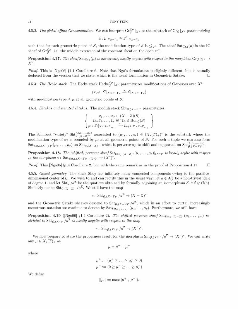
4.5.2. The global affine Grassmannian. We can interpret Gr≤µG |X◦ as the substack of GrG |X◦ parametrizing
β : E|XS−Γx∼= E0|XS−Γx
such that for each geometric point of S, the modification type of β is ≤ µ. The sheaf SatGrG (µ) is the ICsheaf of Gr≤µG , i.e. the middle extension of the constant sheaf on the open cell.
Proposition 4.17. The sheaf SatGrG (µ) is universally locally acyclic with respect to the morphism GrG |X◦ →X◦.
Proof. This is [Ngo06] §1.1 Corollaire 6. Note that Ngô’s formulation is slightly different, but is actuallydeduced from the version that we state, which is the usual formulation in Geometric Satake. �
4.5.3. The Hecke stack. The Hecke stack Hecke≤µG |X◦ parametrizes modifications of G-torsors over X◦
(x, ϕ : E ′|X×S−Γx∼−→ E|X×S−Γx)
with modification type ≤ µ at all geometric points of S.
4.5.4. Shtukas and iterated shtukas. The moduli stack ShtG,(X−Z)r parametrizesx1, . . . , xr ∈ (X − Z)(S)
E0, E1, . . . , Er ∼= σE0 ∈ BunG(S)
ϕi : Ei|X×S−Γxi+1
∼−→ Ei+1|X×S−Γxi+1
The Schubert “variety” Sht
≤(µ1,...,µr)G,(X−Z)r associated to (µ1, . . . , µr) ∈ (X∗(T )+)r is the substack where the
modification type of ϕi is bounded by µi at all geometric points of S. For such a tuple we can also formSatShtG ,(X−Z)r (µ1, . . . , µr) on ShtG,(X−Z)r , which is perverse up to shift and supported on Sht
≤(µ1,...,µr)G,(X−Z)r .
Proposition 4.18. The (shifted) perverse sheaf SatShtG ,(X−Z)r (µ1, . . . , µr)|(X◦)r is locally acylic with respectto the morphism π : SatShtG ,(X−Z)r |(X◦)r → (X◦)r.
Proof. This [Ngo06] §1.4 Corollaire 2, but with the same remark as in the proof of Proposition 4.17. �
4.5.5. Global geometry. The stack ShtG has infinitely many connected components owing to the positive-dimensional center of G. We wish to and can rectify this in the usual way: let a ∈ A×F be a non-trivial ideleof degree 1, and let ShtG /a
Z be the quotient obtained by formally adjoining an isomorphism E ∼= E ⊗O(a).Similarly define ShtG,(X−Z)r /a
Z. We still have the map
π : ShtG,(X−Z)r /aZ → (X − Z)r
and the Geometric Satake sheaves descend to ShtG,(X−Z)r /aZ, which in an effort to curtail increasingly
monstrous notation we continue to denote by SatShtG,(X−Z)r(µ1, . . . , µr). Furthermore, we still have:
Proposition 4.19 ([Ngo06] §1.4 Corollaire 2). The shifted perverse sheaf SatShtG ,(X−Z)r (µ1, . . . , µr) re-stricted to ShtG,(X◦)r /a
Z is locally acyclic with respect to the map
π : ShtG,(X◦)r /aZ → (X◦)r.
We now prepare to state the properness result for the morphism ShtG,(X◦)r /aZ → (X◦)r. We can write
any µ ∈ X∗(T )+ asµ = µ+ − µ−
where
µ+ := (µ+1 ≥ . . . ≥ µ+
r ≥ 0)
µ− := (0 ≥ µ−1 ≥ . . . ≥ µ−r )
We define||µ|| := max(|µ+|, |µ−|).

NEARBY CYCLES OF PARAHORIC SHTUKAS, AND A FUNDAMENTAL LEMMA FOR BASE CHANGE 15
Proposition 4.20 ([Ngo06] §1.6 Proposition 2). Let (µ1, . . . , µr) ∈ (X∗(T )+)r. Suppose that the locus Z oframification points of D satisfies
#Z ≥ n2(||µ1||+ . . .+ ||µr||).Then the morphism
π◦ : Sht≤(µ1,...,µr)G,(X◦)r /aZ → (X◦)r
is proper.
We need to extend this result to our integral model X − Z = X◦ ∪ {x0}.
Proposition 4.21. Let (µ1, . . . , µr) ∈ (X∗(T )+)r. Suppose that the locus Z of ramification points of Dsatisfies
#Z ≥ n2(||µ1||+ . . .+ ||µr||).Then the morphism
π : Sht≤(µ1,...,µr)G,(X−Z)r /aZ → (X − Z)r
is proper.
Proof. Let G be the group scheme isomorphic to G at places away from x0 but hyperspecial at x0. ThenProposition 4.20 applied to ShtG shows that
π′ : Sht≤(µ1,...,µr)G,(X−Z)r /aZ → (X − Z)r
is proper. The map G → G induces a projection
pr: Sht≤(µ1,...,µr)G,(X−Z)r /aZ → Sht
≤(µ1,...,µr)G,(X−Z)r /aZ
which we claim is proper. It obviously suffices to prove the claim. For that we consider the commutativediagram below, omitting some subscripts and superscripts, etc. for clarity of presentation.
ShtG BunG
HeckeG BunG ×BunG
ShtG BunG
HeckeG BunG×BunG
Id×Frob
h←×h→
Id×Frob
h←×h→
In this diagram the squares with solid arrows are cartesian. Let Hecke′G and Sht′G denote the fibered products
Hecke′G BunG ×BunG
HeckeG BunG×BunG
h←×h→
h←×h→
andSht′G BunG
Hecke′G BunG ×BunG
Id×Frob
h←×h→
.
The map BunG → BunG is proper, hence so is pullback Hecke′G →→ HeckeG. Since the map Hecke≤(µ1,...,µr)G →
(Hecke′G)≤(µ1,...,µr) is proper, the map Sht≤(µ1,...,µr)G → Sht
′≤(µ1,...,µr)G is also proper, hence so is the compo-
sitionSht≤(µ1,...,µr)G → (Sht′G)
≤(µ1,...,µr) pr−→ Sht≤(µ1,...,µr)
G .
�

16 TONY FENG
5. The Kottwitz Conjecture for shtukas
5.1. Parahoric Hecke algebras. Let G be a split reductive group over a non-archimedean local field Ftwith uniformizer t. (The splitness assumption is not necessary, but is certainly adequate for our eventualpurposes and simplifies the notation significantly.)
5.1.1. Spherical Hecke algebra. Let K be a hyperspecial maximal compact subgroup of G(Ft). By Bruhat-Tits theory we may extend G to an integral model over the valuation subring Ot ⊂ Ft such that G(Ot) = K.
Let HG,K = Func(K\G(Ft)/K,Q`) be the corresponding spherical Hecke algebra. This has severalcanonical bases, so we fix notation for them. Let T ⊂ G be a maximal split torus. As is well known, we havea Cartan decomposition
G(Ft) =⋃
µ∈X∗(T )+
KtµK (5.1)
indexed by the dominant coweights X∗(T )+∼= Zn, where tµ is the character such that for a character
χ ∈ X∗(T ), we have χ(tµ) = t〈χ,µ〉.
Definition 5.1. For µ ∈ X∗(T )+, we denote by fµ ∈ HG,K the indicator function of KtµK.
5.1.2. Geometrization of spherical Hecke algebra. A second basis is obtained by interpreting categorifyingthe Hecke algebra in terms of L+G-equivariant perverse sheaves on the affine Grassmannian GrG. Recallthat GrG(kt) = G(Ft)/G(Ot) where kt is the residue field of Ft. Geometric Satake furnishes a symmetricmonoidal equivalence
PervG(Ot)(GrG) ∼= Rep(G).
The simple objects in Rep(G) are indexed by µ ∈ X∗(T )+, and we denote by SatGrG(µ) the correspondingperverse sheaf on GrG, which is the IC sheaf of the Schubert variety Gr≤µG .
For any F ∈ PervG(Ot)(GrG), we have under the function-sheaf dictionary ([KW01] §III.12) a tracefunction fF on G(Ot)\G(Ft)/G(Ot) given by
fF (x) = Tr(Frob,Fx). (5.2)
Definition 5.2. We define ψµ to be the trace function associated to SatGrG(µ).
Definition 5.3. Since SatGrG (µ) is a G(Ox0)-equivariant sheaf on GrG,x0
, its stalks are the same on anyopen Schubert cell Gr=ν corresponding to KtνK in the Cartan decomposition (5.1). We denote this commonstalk by SatGrG(µ)ν .
Lemma 5.4. We haveψµ =
∑ν≤u
Tr(Frob,SatGrG(µ)ν)fν
Proof. This is immediate from the fact that SatGr(µ)ν is supported on Gr≤µ, which is the union of the Gr=ν
for ν ≤ µ, and the definition of fν as the characteristic function on KtνK. �
We have a Satake isomorphism
HG(K)∼−→ R(G) ∼= Q`[X∗(T )]W
where W is the Weyl group of T . (The Satake isomorphism is reviewed in §7.2.) Here R(G) is the represen-tation ring of G, which is generated by the classes of the highest weight representations Vµ.
5.1.3. Parahoric Hecke algebras. Let J be a parahoric subgroup ofG stabilizing a facet in the dominant alcoveof the vertex corresponding to K in the Bruhat-Tits building of G(Ft). Let HG,J = Func(J\G(Ft)/J,Q`)be the corresponding parahoric Hecke algebra.
Theorem 5.5 (Bernstein, [Hai09] Theorem 3.1.1.). Convolution with f0 = IK (the identity of HG,K) inducesan isomorphism
− ∗J IK : Z(HG,J)∼−→ HG,K .
Definition 5.6. For µ ∈ X∗(T )+,• We denote by f ′µ the unique element of Z(HG,J) such that f ′µ ∗ IK = fµ.• We denote by ψ′µ ∈ Z(HG,J) the unique element such that ψ′µ ∗ IK = ψµ ∈ HG,K .

NEARBY CYCLES OF PARAHORIC SHTUKAS, AND A FUNDAMENTAL LEMMA FOR BASE CHANGE 17
5.1.4. Geometrization of parahoric Hecke algebras. There is a geometrization of the parahoric Hecke algebracompletely analogous to §5.1.2. Let G be the parahoric group scheme corresponding to J by Bruhat-Titstheory. Then the Hecke algebra HG,J is categorified by PervG(O)(GrG).
Note that if J = I is an Iwahori subgroup (the stabilizer of full alcove), then GrG is the affine flag varietyFlG. In general one can think of GrG as a kind of affine partial flag variety.
One might ask which sheaves the functions ψ′µ correspond to. The answer is that they can be realized asnearby cycles of certain global degenerations, and it is the key point underlying this section.
5.2. Nearby cycles. We recall the definition and essential (for us) properties of the nearby cycles functor.For a reference, see [Del73] Exposé XIII.
A Henselian trait is a triple (S, s, η) where S is a the spectrum of a discrete valuation ring, s is the specialpoint of S and η is the generic point of S. Choose geometric points s and η lying over s and η, respectively.Let S be the normalization of S in η. We denote by
i : s ↪→ S
j : η ↪→ S
i : s→ S
j : η → S
the obvious maps.Let f : Y → S be a finite type scheme over S. One defines a topos Y ×s η as in [Del73] Exposé XIII
§1.2, so that the category Dbc(Y ×s η,Q`) is the category of F ∈ Db
c(Y ×s s,Q`) together with a continuousGal(η/η)-action compatible with the Gal(s/s)-action on Ys via the natural map Gal(η/η)→ Gal(s/s).
Definition 5.7. Given F ∈ Dbc(Yη,Q`) we define the nearby cycles RΨ(F) ∈ Db
c(Y ×s s,Q`) by
RΨ(F) := i∗Rj∗(Fη)
with the Gal(η/η)-action obtained by transport of structure from that on Fη.
Remark 5.8. When the nearby cycles construction is performed with S = Spec Fq[[t]], the sheaf RΨ(F)
is a priori only defined over YFq , but can be descended to YFq by choosing a splitting Gal(Fq/Fq) →Gal(Fq((t))/Fq((t))). When dealing with nearby cycles on affine Grassmannians (or related objects) this isoften what we mean (see [Gai01], Footnote 4 on page 8). Only after such a descent one can associate a tracefunction to RΨ(F). We shall point out when this descent is being used, but as a blanket rule it is necessaryevery time we wish to talk about a trace function.
Lemma 5.9. If f : Y → S is proper, then the base change homomorphism
RΨf∗ → f∗RΨ
is an isomorphism.
Proof. This is [Del73], Exposé XIII (2.1.7.1). �
Corollary 5.10. If f : Y → S is proper, then the natural map
Hic(Yη,Q`)→ Hi
c(Ys, RΨ(Q`)).
is an isomorphism.
Lemma 5.11. If f : Y → S is lisse, then the base change homomorphism
f∗RΨ→ RΨf∗
is an isomorphism.
Proof. This is [Del73], Exposé XIII (2.1.7.2). �

18 TONY FENG
5.3. Degeneration to affine flag varieties. Let X be a smooth curve (not necessarily projective) over Fqand let G → X be a parahoric group scheme, with parahoric level structure at x0. We consider the globalaffine Grassmannian for G as in §4.1:
π : GrG → X.
Consider the restriction GrG |Dx0, where Dx0 := Spec Ox0 is the spectrum of the completed local ring at x0.
We apply the nearby cycles construction of §5.2 and in the form of Remark 5.8, to• S = Dx0
, Y = GrG |Dx0, and
• F = SatGrG (µ)|D∗x0, where D∗x0
= Spec Fx0is thought of as a local “punctured disk” around x0.
This produces a G(Ox0)-equivariant perverse sheaf RΨ(SatGrG (µ)|D◦x0
) on GrG |x0, which we will abbreviate
by RΨ(SatGrG (µ)).
Theorem 5.12 (Gaitsgory [Gai01], Zhu [Zhu14]). The sheaf RΨ(SatGrG (µ))) is central.
Remark 5.13. In the present formulation and level of generality, this theorem is actually due to X. Zhu in[Zhu14] Theorem 7.3. Gaitsgory worked with constant group schemes G, and a slightly different degeneration.
Corollary 5.14. Assume that G := G|Fx0is split. Then the trace function (in the sense of (5.2)) associated
to RΨ(SatGrG (µ))) is ψ′µ (Definition 5.6).
Remark 5.15. Note that we need to use Remark 5.8 to descend RΨ(SatGrG (µ))) to GrG |x0 , so that itmakes sense to speak of the trace function.
Proof. Since RΨ(SatGrG (µ)) is a G(Ox)-equivariant perverse sheaf on GrG |x0, which is central by Theorem
5.12, we have a priori that its trace function
Tr(Frob, RΨ(SatGrG (µ)))
lies in Z(HG,G(Ox0)(Fx)). Since G is split we can extend it to a constant group scheme over Dx0 , which we
continue to denote G, such that G0(Ox0) =: K is a hyperspecial maximal compact subgroup of G(Fx). Write
also J := G(Ox0) for the parahoric subgroup. By the Bernstein isomorphism (Theorem 5.5)
− ∗ IK : Z(HG,J)∼−→ HG,K
it suffices to check thatTr(Frob, RΨ(SatGrG (µ))) ∗ IK = ψµ. (5.3)
By [Gai01] Theorem 1 (d) the map (5.3) is realized sheaf-theoretically by the pushforward via the propermap
pr: GrG → GrG
or in other words,Tr(Frob, RΨ(SatGrG (µ))) ∗ IK = Tr(Frob,pr!RΨ(SatGrG (µ))).
Now, by Lemma 5.9 and the fact that pr is an isomorphism over D∗x0(since G|D∗x0
∼= G|D∗x0) we have
pr!RΨ(SatGrG (µ)) = RΨ(SatGrG(µ))
but since G0|Dx → Dx is smooth with constant fiber GrG, we simply have
RΨ(SatGrG(µ)) = SatGrG(µ)|x0 ,
whose trace function is ψµ by definition. �
Schubert stratification. Let GrG,x0be the fiber of GrG over x0. We discuss the stratification induced by the
G(Ox0)-action on GrG,x0
.The analogue of the Cartan decomposition (5.1) is
G(Ox0)\G(Fx0
)/G(Ox0) ∼= WJ\W/WJ
where W is the extended affine Weyl group, and WJ is the subgroup corresponding to the parahoric subgroupJ := G(Ox0
). We refer to [Hai09] §2.6 for the notation and definitions; all that we require are the followingabstract facts:
• The G(Ox0)-orbits on GrG,x0 are indexed by ν ∈ WJ\W/WJ . We denote the open orbit correspondingto ν ∈ WJ\W/WJ by Gr=ν
G,x0and its closure by Gr≤νG,x0
.

NEARBY CYCLES OF PARAHORIC SHTUKAS, AND A FUNDAMENTAL LEMMA FOR BASE CHANGE 19
• There is a partial order on WJ\W/WJ such that µ ≥ ν if and only if Gr≤µG,x0⊃ Gr=ν
G,x0.
Definition 5.16. Since RΨ(SatGrG (µ)) is a J-equivariant perverse sheaf on GrG,x0([Gai01] Theorem 1), its
stalks are the same on any open Schubert cell Gr=νG . We denote this common stalk by RΨ(SatGr(µ))ν .
Lemma 5.17. We have
ψ′µ =∑ν≤µ
Tr(Frob, RΨ(SatGrG (µ))ν)fν
Proof. The argument is the same as for Lemma 5.4. �
5.4. Local models for shtukas.
Definition 5.18. Let X and Y be Artin stacks. We say that Y is an étale local model for X if there existsan Artin stack W and a diagram
W
X Y
étalef
étaleg
A diagram as above is called a local model diagram.
Theorem 5.19 (Varshavsky, V. Lafforgue). The stack Gr≤(µ1,...,µr)G,Xr is an étale local model for Sht
≤(µ1,...,µr)G .
Remark 5.20. This is a variation on well-known results, which are not quite stated in the literature atthe level of generality needed here. Varshavsky proved this ([Var04] Theorem 2.20) for a constant groupG = G×X, while the general case is essentially implicit in [Laf12], so we credit it to both of them.
Proof. For ease of presentation, we assume that r = 1 in the proof; the argument for the general case isa completely straightforward generalization. Since for any given µ the L+G-action on Hecke≤µG and Gr≤µGfactors through a finite étale quotient, Proposition 4.8 implies that there is an étale cover Hecke≤µG,N →Hecke≤µG , obtained by adding a finite level structure, equipped with an étale map Hecke≤µG,N → Gr≤µG ×BunG .
Define Sht≤µG,N by the cartesian diagram
Sht≤µG,N BunG
Hecke≤µG,N BunG ×BunG
Id×Frob
h←×h→
Then we have a finite étale cover Sht≤µG,N → Sht≤µG , which concretely is the covering map for a finite levelstructure. This fits into a diagram
Sht≤µG,N BunG
Sht≤µG Hecke≤µG,N BunG ×BunG
BunG ×Gr≤µG
étaleId×Frob
étale
h←×h→ (5.4)
It is a general fact that in this situation that the vertical composition Sht≤µG,N → Gr≤µG is étale. Indeed, sincethe claim is local in the smooth topology, we may perform a base change to make everything into a scheme,and apply [Laf12] Lemma 2.13 to W = Hecke≤µG,N , T = Gr≤µG , and Z = BunG . �

20 TONY FENG
Corollary 5.21. Let µ ∈ X∗(T )r. There is an étale local model diagram
W≤µ
Sht≤µG Gr
≤µG
Xr
étalef
étaleg
withf∗ SatShtG (µ) = g∗ SatGrG (µ).
Proof. This follows from the diagram (5.4) and the definition of the Satake sheaves, taking W≤µ = Sht≤µG,N .�
Let µ ∈ X∗(T )r. By Corollary 5.21, we may set
SatW(µ) := f∗ SatShtG (µ) = g∗ SatGrG (µ).
We write RΨx0to emphasize that we are taking nearby cycles over the point x0. By Lemma 5.11, and
implicitly using Corollary 5.21, we have
f∗RΨx0(SatShtG (µ)) = RΨx0(SatW(µ)) = g∗RΨx0(SatGrG (µ)).
Thus, for w ∈ W(k) lying over y ∈ ShtG(k) and z ∈ GrG(k), we have
Tr(Frob, RΨx0(SatShtG (µ))y) = Tr(Frob, RΨx0(SatW(µ))w) = Tr(Frob, RΨx0(SatGrG (µ))z).
Therefore, the stalks of RΨx0(SatShtG (µ)) are constant along the stratification
Sht≤µG =
∐ν≤µ
Sht=νG ,
and we deduce:
Corollary 5.22. For ν ∈ X∗(T )+, we have
Tr(Frob, RΨx0(SatShtG (µ))ν) = Tr(Frob, RΨx0(SatGrG (µ))ν).
Remark 5.23. We will actually need to work with ShtG /aZ instead. Since this is obtained from ShtG by
gluing isomorphic components, the result is exactly the same.
6. Counting parahoric shtukas
Our eventual goal is establish a formula for the trace of an operator, formed as a composition of Heckeoperators and Frobenius, on the cohomology of the nearby cycles sheaf of (a variant of) ShtG /a
Z → X, ata place of parahoric bad reduction. The mold for such calculations was set by Kottwitz in [Kot92], whocomputed this sort of trace for certain PEL Shimura varieties, at places of good (hyperspecial) reduction. Ithas since been extended vastly by work of many authors; we note that in particular that Kisin and Pappasconstructed integral models for Shimura varieties with parahoric level structure and computed the trace ofFrobenius on nearby cycles in [KP]. Our result is a function field analogue of this computation.
In this section we carry out one step of this calculation, which deals with counting the number of fixedpoints of Frobenius composed with Hecke correspondences. (The precise setup will be explained in §6.1.) Infact most of the work has already been done by B.C. Ngô and T. Ngô Dac, who studied the case of moduliof shtukas with hyperspecial reduction in the series of papers [Ngo06], [NND08], [ND13], and [ND15]. Theonly new element here is that we are considering parahoric reduction. We note also that our results shouldfollow from work of Hartl and Arasteh Rad proving the analogue of the Langlands-Rapoport Conjecture forshtukas [HRb].
NEARBY CYCLES OF PARAHORIC SHTUKAS, AND A FUNDAMENTAL LEMMA FOR BASE CHANGE 21
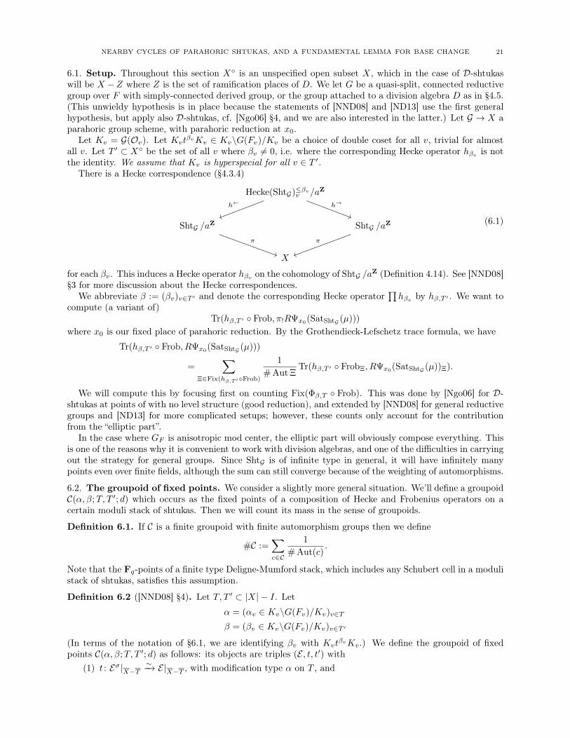
6.1. Setup. Throughout this section X◦ is an unspecified open subset X, which in the case of D-shtukaswill be X −Z where Z is the set of ramification places of D. We let G be a quasi-split, connected reductivegroup over F with simply-connected derived group, or the group attached to a division algebra D as in §4.5.(This unwieldy hypothesis is in place because the statements of [NND08] and [ND13] use the first generalhypothesis, but apply also D-shtukas, cf. [Ngo06] §4, and we are also interested in the latter.) Let G → X aparahoric group scheme, with parahoric reduction at x0.
Let Kv = G(Ov). Let KvtβvKv ∈ Kv\G(Fv)/Kv be a choice of double coset for all v, trivial for almost
all v. Let T ′ ⊂ X◦ be the set of all v where βv 6= 0, i.e. where the corresponding Hecke operator hβv is notthe identity. We assume that Kv is hyperspecial for all v ∈ T ′.
There is a Hecke correspondence (§4.3.4)
Hecke(ShtG)≤βvv /aZ
ShtG /aZ ShtG /a
Z
X
h← h→
π π
(6.1)
for each βv. This induces a Hecke operator hβv on the cohomology of ShtG /aZ (Definition 4.14). See [NND08]
§3 for more discussion about the Hecke correspondences.We abbreviate β := (βv)v∈T ′ and denote the corresponding Hecke operator
∏hβv by hβ,T ′ . We want to
compute (a variant of)Tr(hβ,T ′ ◦ Frob, π!RΨx0(SatShtG (µ)))
where x0 is our fixed place of parahoric reduction. By the Grothendieck-Lefschetz trace formula, we have
Tr(hβ,T ′ ◦ Frob, RΨx0(SatShtG (µ)))
=∑
Ξ∈Fix(hβ,T ′◦Frob)
1
# Aut ΞTr(hβ,T ′ ◦ FrobΞ, RΨx0
(SatShtG (µ))Ξ).
We will compute this by focusing first on counting Fix(Φβ,T ◦ Frob). This was done by [Ngo06] for D-shtukas at points of with no level structure (good reduction), and extended by [NND08] for general reductivegroups and [ND13] for more complicated setups; however, these counts only account for the contributionfrom the “elliptic part”.
In the case where GF is anisotropic mod center, the elliptic part will obviously compose everything. Thisis one of the reasons why it is convenient to work with division algebras, and one of the difficulties in carryingout the strategy for general groups. Since ShtG is of infinite type in general, it will have infinitely manypoints even over finite fields, although the sum can still converge because of the weighting of automorphisms.
6.2. The groupoid of fixed points. We consider a slightly more general situation. We’ll define a groupoidC(α, β;T, T ′; d) which occurs as the fixed points of a composition of Hecke and Frobenius operators on acertain moduli stack of shtukas. Then we will count its mass in the sense of groupoids.
Definition 6.1. If C is a finite groupoid with finite automorphism groups then we define
#C :=∑c∈C
1
# Aut(c).
Note that the Fq-points of a finite type Deligne-Mumford stack, which includes any Schubert cell in a modulistack of shtukas, satisfies this assumption.
Definition 6.2 ([NND08] §4). Let T, T ′ ⊂ |X| − I. Letα = (αv ∈ Kv\G(Fv)/Kv)v∈T
β = (βv ∈ Kv\G(Fv)/Kv)v∈T ′
(In terms of the notation of §6.1, we are identifying βv with KvtβvKv.) We define the groupoid of fixed
points C(α, β;T, T ′; d) as follows: its objects are triples (E , t, t′) with(1) t : Eσ|X−T
∼−→ E|X−T , with modification type α on T , and

22 TONY FENG
(2) t′ : Eσd |X−T ′∼−→ E|X−T ′ , with modification type β on T ′,
(3) satisfying the following compatibility:
Eσd+1 |X−T−T ′ Eσd |X−T−T ′
Eσ|X−T−T ′ E|X−T−T ′
σd(t)
σ(t′) t′
t
The automorphisms of (E , t, t′) are defined to be automorphisms of E commuting with t and t′.
The relation to our initial problem is given by the following.
Lemma 6.3. Suppose x ∈ |X| is a point of degree d. Then we have an isomorphism of groupoids
Fix(hβ,T ′ ◦ Frob,Sht=µG |x) ∼= C(µ, β; {x}, T ′; d).
Proof. This is immediate upon writing down the definitions. �
We actually want to study the truncated space Sht=µG /aZ, so we modify the discussion accordingly. Let
J ⊂ Z(G)(A) be a cocompact lattice. Then J acts on Sht=µG via Hecke correspondences, and we define
Sht=µG /J to be the quotient. Similarly we define C(µ, β; {x}, T ′; d)J to be the quotient by the J-action. (See
[NND08], near the end of §4, for more details.)
Lemma 6.4. Suppose x ∈ |X| is a point of degree d. Then we have an isomorphism of groupoids
Fix(hβ,T ′ ◦ Frobx,Sht=µG /J |x) ∼= C(µ, β; {x}, T ′; d)J .
Hence we want to study #C(µ, β; {x}, T ′; d)J . The strategy for these counts goes back to Kottwitz’s studyof points of Shimura varieties (with hyperspecial level structure) over finite fields [Kot92].
(1) We first show that there is a cohomological invariant, the Kottwitz invariant, which controls thepossible “generic fibers” of members of C(α, β;T, T ′; d).
(2) We then express the size of an isogeny class as a product of (twisted) orbital integrals.(3) We then express the number of isogeny classes associated to each Kottwitz invariant in terms of
certain cohomology groups.These steps have been carried out in papers of B.C. Ngô and T. Ngô Dac, as already mentioned, but notquite in the generality required here. In particular, these previous papers avoid the case where T meets apoint with non-trivial level structure (because the moduli problem was not defined over such points), whichis exactly the situation that we are interested in. So we will describe the modifications needed to extendthe argument to our setting, and only briefly summarize the parts that are already covered in the papers ofB.C. Ngô and T. Ngô Dac.
6.3. Kottwitz triples and classification of generic fibers. Our first step is to define a category thatlooks like the category of “generic fibers of C(α, β;T, T ′; d)”.
Definition 6.5 ([NND08] §5). Let T, T ′ ⊂ |X|−I. We define the groupoid C(T, T ′; d) as follows: its objectsare triples (V, τ, τ ′) with
(1) V a G-torsor over Fk := F ⊗k k,(2) an isomorphism τ : V σ
∼−→ V , where V σ = V ⊗Fk,σ Fk,(3) τ ′ : V σ
d ∼−→ V ,satisfying the following conditions:
(1) (“commutativity”) The following diagram commutes:
V σd+1
V σd
V σ E
σd(τ)
σ(τ ′) τ ′
τ
(2) For x /∈ T , (Vx, τx) is isomorphic to the trivial isocrystal (G(Fx⊗FqFq), Id ⊗Fqσ).(3) For x ∈ T , (Vx, τ
′x) is isomorphic to the trivial isocrystal (G(Fx⊗FqFq), Id ⊗F
qdσd).

NEARBY CYCLES OF PARAHORIC SHTUKAS, AND A FUNDAMENTAL LEMMA FOR BASE CHANGE 23
The automorphisms of (V, τ, τ ′) are automorphisms of E commuting with τ and τ ′.
The operation of “taking the generic fiber” defines a functor ([NND08] §5.2)
C(α, β;T, T ′; d)→ C(T, T ′; d).
6.3.1. Kottwitz triples. Recall that a Kottwitz triple is a datum (γ0, (γx)x/∈T , (δx)x∈T ) where:• γ0 is a stable conjugacy class of G(F ),• γx is a conjugacy class of G(Fx) for each x /∈ T , and is stably conjugate to γ0,• δx is a σ-conjugacy class of G(Fx⊗FqFqd), whose norm
N(δx) := δx · σ(δx) · . . . · σd−1(δx)
is stably conjugate to γ0.
Construction 6.6. We now recall from [NND08] §6.1 how to attach to each (V, τ, τ ′) ∈ C(T, T ′; d) aKottwitz triple (γ0, (γx)x/∈T , (δx)x∈T ).
First a remark on notation: for a map τ : V σ → V , we denote by τn : V σn → V the map τ ◦ σ(τ) ◦ . . . ◦
σn−1(τ).(1) Definition of γ0. Since Fk has cohomological dimension 1, the G-torsor V is split over Fk. Consider
γ = τd(τ ′)−1, which is a linear automorphism of V . Using the “commutativity” axiom we find that
σ(γ) = σ(τ) ◦ σ2(τ) ◦ . . . ◦ σd(τ) ◦ σ(τ ′)−1 = τ−1γτ.
This shows that the conjugacy class of γ is stable under σ, hence defined over F . Since G wasassumed to be quasi-split with simply connected derived subgroup, this conjugacy class must thencontain an F -point. Thus, we have an element γ0 ∈ G(F ) with a well-defined stable conjugacy class.
(2) Definition of γx, x /∈ T . By assumption, we can pick an isomorphism
(Vx, τx) ∼= (G(Fx⊗FqFq), Id ⊗Fqσ).
Since τ and τ ′ commute, so do τx and τ ′x, so that τ ′x defines an automorphism of (G(Fx⊗FqFq), Id ⊗Fqσ).We can then write τ ′x = γ−1
x ⊗ σd, for some γx ∈ G(Fx) which is stably conjugate to γ0. (The pointis that picking this trivialization of τx amounts to setting “τx = Id” in the equation γx = τdx (τ ′x)−1.)
(3) Definition of δx, x ∈ T . By assumption, we can pick an isomorphism
(Vx, τ′x) ∼= (G(Fx⊗FqFq), Id ⊗Fdq
σd).
Since τ and τ ′ commute, so do τx and τ ′x, so that τx defines an automorphism of (G(Fx⊗FqFq), Id ⊗Fqσ).We can then write τx = δx ⊗ σ, for some δx ∈ G(Fx), well-defined up to σ-conjugacy, whose normN(δx) = δx · σ(δx) · . . . · σr−1(δx) is stably conjugate to γ0.
Definition 6.7. We say that (V, τ, τ ′) ∈ C(T, T ′; d) is semisimple if γ0 is semisimple, and elliptic if γ0 iselliptic.
We say (E , t, t′) ∈ C(α, β;T, T ′; d) is semisimple (resp. elliptic) if the associated (V, τ, τ ′) is semisimple(resp. elliptic).
6.3.2. The Kottwitz invariant. Following [NND08] §6.2 we can attach to the Kottwitz triple (γ0, (γx), (δx))
a character inv(γ0, (γx), (δx)) ∈ X∗(Z(Gγ0)Γ). Briefly, this is done as follows.• For x /∈ T , since γx and γ0 are stably conjugate, by a theorem of Steinberg we can find g ∈ G(Fx⊗kk)
such thatgγ0g
−1 = γx.
Then (using that γ0 ∈ G(F )) we have
gγ0g−1 = γx = σ(γx) = σ(g)γ0σ(g)−1.
This shows that g−1σ(g) is in the centralizer of γ0 in G(Fx⊗kk), hence defines a class in B(Gγ0,x) =
G(Fx⊗kk)/σ-conjugacy.• For x ∈ T , we have g ∈ G(Fx⊗kk) such that Nδx = gγ0g
−1. Then g−1δxσ(g) is in Gγ0(Fx⊗kk) anddefines a class in B(Gγ0,x).

24 TONY FENG
For each x, we apply the mapB(Gγ0,x)→ X∗(Z(Gγ0)Γx) of [Kot90] §6 to get a local character invx(γ0, (γx), (δx)) ∈X∗(Z(Gγ0
)Γx). Almost all of the resulting characters are trivial, so that it makes sense to sum the restrictionsof all these characters to Z(Gγ0
)Γ, and we define this sum to be inv(γ0, (γx), (δx)).
Proposition 6.8. [NND08] For elliptic (V, τ, τ ′) ∈ C(T, T ′; d), and (γ0, (γx), (δx)) the associated Kottwitztriple, if γ0 is semisimple then we have inv(γ0, (γx), (δx)) = 0.
Proposition 6.9. There exists (V, τ, τ ′) ∈ C(T, T ′; d) having a given elliptic Kottwitz triple (γ0, (γx), (δx))if and only if inv(γ0, (γx), (δx)) = 0. If the set of such is non-empty, then the number of isogeny classeswithin C(T, T ′; d) having the same Kottwitz triple is the cardinality of
ker1(F,Gγ0) := ker(H1(F,Gγ0)→∏x
H1(Fx, Gγ0)).
Proof. This follows from the proof of [NND08] Proposition 11.1 combined with [ND13] Proposition 4.3. �
6.3.3. Automorphisms of the generic fiber. Let (V, τ, τ ′) ∈ C(T, T ′; d) with elliptic Kottwitz triple (γ0, (γx), (δx)).By [ND13] §3.9, the automorphisms of (V, τ, τ ′) are the Fx-points of an inner form Jγ0
of Gγ0defined over
F .
Remark 6.10. As pointed out in [ND13] §3.9, the Hasse principle implies that Jγ0 is determined by itslocal components:
• For x /∈ T , Jγ0,x is the centralizer of γx in G(Fx),• For x ∈ T , Jγ0,x is the twisted centralizer of δx in G(Fx ⊗Fq Fqd).
6.4. Counting lattices. We now study the fibers of the functor C(α, β;T, T ′; d)→ C(T, T ′; d).
Proposition 6.11. Fix an elliptic (V, τ, τ ′) ∈ C(T, T ′; d). Suppose (E , t, t′) ∈ C(α, β;T, T ′; d) lies over(V, τ, τ ′). The size of the isogeny class of (E , t, t′) is
vol(J · Jγ0(F )\Gγ0
(A)) ·∏x/∈T
Oγx(φβx)∏x∈T
TOδxσ(φαx).
Here we normalize Haar measures as in §2.1.1.
Proof. Promoting (V, τ, τ ′) to (E , t, t′) amounts to choosing a Gx⊗kk-bundle over Spec Ox for all x ∈ X, plusan I-level structure, such that
• for v /∈ |T |, Ex is fixed by τ ,• for v /∈ |T |′, Ex is fixed by τ ′,• for x ∈ |T |, the relative position of Ex and τ(Ex) is given by αx,• for v ∈ |T |′ (hence outside |T |), the relative position of Ev and τ ′(Ev) is given by βv.
As is well-known (cf. [NND08] §9 or [ND13] §5 for the present situation; the earliest reference we know is[Kot80]), this is counted by∫
J·Jγ0 (F )\∏x∈T G(Fx⊗FqFqd )×G(AT )
⊗x∈T
φαx(h−1x δxσ(hx))
⊗x/∈T
φβx(h−1x γxhx) dh.
Here we use Remark 6.10 to view Jγ0(F ) as a subset of G(Fx). The statement of the proposition is a
straightforward rewriting of this formula. �
6.5. Count of elliptic elements. Define
#C(α, β;T, T ′; d)ell :=∑
(E,t,t′) elliptic
1
# Aut(E , t, t′).
Combining Proposition 6.9, §6.3.3, and Proposition 6.11, we obtain:

NEARBY CYCLES OF PARAHORIC SHTUKAS, AND A FUNDAMENTAL LEMMA FOR BASE CHANGE 25
Theorem 6.12. We have
#C(α, β;T, T ′; d)ell =∑
(γ0,(γx),(δx))inv(γ0,(γx),(δx))=0
γ0 elliptic
ker1(F,Gγ0) · vol(J · Jγ0
(F )\Jγ0(AF )) · dg(K)−1
·
(∏x/∈T
Oγx(fβv )
) ∏x∈|T |
TOδxσ(fαx)
Remark 6.13. This is the analogue of [ND13] Théorème 5.1. The expressions look almost the same, butone should keep in mind that in our applications T = {x0}, and fαx0
should be thought of as an indicatorfunction on a partial affine flag variety rather than an affine Grassmannian. In addition, the measure of Kx0
is adapted accordingly.
Corollary 6.14. Let Sht≤µG /aZ be the moduli stack of D-shtukas with parahoric level structure at x0, as in§4.5. Then
# Fix(hβ,T ′ ◦ Frob,Sht=µG /aZ|x0) =
∑(γ0,(γx),(δx))
inv(γ0,(γx),(δx))=0
ker1(F,Gγ0) · vol(aZ · Jγ0(F )\Jγ0(AF ))·
· dg(K)−1 ·
(∏x/∈T
Oγx(fβv )
)· TOδx0
σ(fµ).
Proof. This is immediate from Lemma 6.4 and the observation that every non-zero element of a divisionalgebra is elliptic, since the associated group of units is anisotropic mod center. (As mentioned at thebeginning of §6, the results used from [NND08] and [ND13] also apply to D-shtukas, and in fact wereoriginally proved for this case in [Ngo06] §4.) �
7. Geometrization of base change for Hecke algebras
In this section we present a geometric interpretation of the base change homomorphism for sphericalHecke algebras, and then for the center of parahoric Hecke algebras. The results here are a generalizationto arbitrary split reductive groups G of results from [Ngo99], which proved the result for GLn.
Using the work of Gaitsgory on realizing central sheaves on the affine flag variety as nearby cycles, wethen deduce a geometric interpretation of base change for the center of the parahoric Hecke algebra.
7.1. Definition of base change homomorphism. For this section only, we let F be a local field and Gbe a reductive group over F . Given a compact open subgroup H ⊂ G(F ), we have the Hecke algebra
HG,H := Func(H\G(F )/H,Q`).
We begin by defining base change homomorphisms for some Hecke algebras with respect to a degree runramified extension of local fields E/F .
For simplicity we assume that G is split over F . (Our results should extend at least to quasi-split Gwithout much difficulty.) We let E/F be the unramified extension of degree r.
Definition 7.1 ([Hai09] §1). Let K ⊂ G(F ) be a hyperspecial maximal compact subgroup. The base changehomomorphism for spherical Hecke algebras (with respect to E/F ) is the homomorphism of C-algebras
HG(E),K → HG(F ),K
characterized by the following property. Let WF be the Weil group of F . For an admissible unramifiedhomomorphism ψ : WF → LG let ψ′ : WE → LG denote the restriction to WE ⊂WF . Let πψ and πψ′ denotethe corresponding representations of G(E) and G(F ) under the Local Langlands Correspondence. Then forany φ ∈ HG(E),K we have
〈trace πψ′ , φ〉 = 〈trace πψ, b(φ)〉
Definition 7.2 ([Hai09] §1). Let J ⊂ K be a parahoric subgroup and IK denote the characteristic functionof K ⊂ G(F ). By a theorem of Bernstein (cf. [Hai09] Theorem 3.1.1), convolution with IK defines anisomorphism
− ∗J IK : Z(HG,J)∼−→ HG,K .

26 TONY FENG
We define the base change homomorphism for parahoric Hecke algebras to be the homomorphism
b : HG(E),J → HG(F ),J
making the following diagram commute:
Z(HG(E),J) Z(HG(F ),J)
HG(E),K HG(F ),K
b
−∗J IK∼ −∗J IK∼
b
(7.1)
7.1.1. Interpretation under Satake isomorphism. Let T ⊂ G be a maximal torus. We have the Satakeisomorphism
S : HG,K∼−→ Q`[X∗(T )]W
where W is the Weyl group of G relative to T . We also have the Bernstein isomorphism
B : Z(HG,J)∼−→ HG,K .
We can define the base change homomorphism on the Satake side as follows. We define the norm homo-morphism
N : Q`[X∗(TE)]W → Q`[X∗(TF )]W
to be that induced by the norm TE → TF . Since we are working in the split setting, this simply correspondsto multiplication by r on X∗(TE)
∼−→ Zn.Then b : HG(E),J → HG(F ),J is determined by the commutativity of the following diagram ([Hai09], §3.2)
Z(HG(E),J) Z(HG(F ),J)
HG(E),K HG(F ),K
C[X∗(TE)]W C[X∗(TF )]W (F )
b
−∗J IK∼ −∗J IK∼
b
S∼ S∼
N
(7.2)
For more on the base change homomorphism, see [Hai09] §3.
7.2. Geometrization of the Satake transform. In this section we will recall a geometric interpretationof the Satake transform.
7.2.1. The classical Satake transform. We first review the Satake transform (cf. [Gro98]). Let HG,K bethe spherical Hecke algebra of G(F ) with respect to a hyperspecial maximal compact subgroup K. LetHT = Q`[X∗(T )].
We choose a Borel subgroup B containing T and let N be its unipotent radical. There is a Sataketransform S : HG,K → HT given by
Sf(t) = δ(t)1/2
∫N
f(tx)dx,
where the Haar measure dx is normalized to assign volume 1 to N(Ot).
Theorem 7.3 (Satake). The Satake transform gives a ring isomorphism
S : HG,K ∼= R(G) ∼= HWTwhere R(G) is the representation ring of G with Q`-coefficients.
We have an isomorphismHT ∼= Q`[X∗(T )].
For λ ∈ X∗(T ), write tλ for the corresponding element of HT . Then we may write
Sf(tλ) = δ(tλ)1/2
∫N
f(tλx)dx. (7.3)

NEARBY CYCLES OF PARAHORIC SHTUKAS, AND A FUNDAMENTAL LEMMA FOR BASE CHANGE 27
7.2.2. Interpretation via semi-infinite orbits. We will interpret the function (7.3) geometrically, as the tracefunction associated to a certain subscheme Sλ, studied by Mirkovic-Vilonen in [MV07] §3, in the sense thatif fF is the trace function associated to F , then
SfF (tλ) = q−ρ(λ) Tr(Frob, RΓc(Sλ ⊗k k,F))
where ρ is the usual half sum of the positive roots.Following the notation of [MV07], for λ ∈ X∗(T ) we let Lλ = tλG(O) denote the image of λ in the affine
Grassmannian GrG, and Sλ be its orbit under NF .
Lemma 7.4. Let F be a sheaf on GrG defined over k, and fF its associated trace function (cf. (5.2)). Thenwe have
SfF (tλ) = q−ρ(λ) Tr(Frob, RΓc(Sλ ⊗k k,F)).
Proof. We study the rational points Sλ(k), in preparation for an application of the Grothendieck-Lefschetztrace formula. The stabilizer of tλ is
StabN(F )(Lλ) = {n ∈ N(F ) : ntλG(O) = tλG(O)}
= {n ∈ N(F ) : t−λntλ ∈ G(O)}.
This says that the map n 7→ t−λntλ defines a bijection between StabN(F )(Lλ) and N(O). Therefore the mapn 7→ tλn defines a bijection between Sλ = [N(F )/StabN(F )(Lλ)] · Lλ and N(F )/N(O). An application ofthe Grothendieck-Lefschetz trace formula then yields
Tr(Frob, RΓc(Sλ ⊗k k,F)) =∑
n∈Sλ(k)
fF (n)
=∑
n∈N(F )/N(O)
fF (tλ · n)
which is exactly what was claimed upon recalling that δ(tλ) = qρ(λ). �
Theorem 7.5 (Mirkovic-Vilonen). There is a natural equivalence of functors
H∗(−) ∼=⊕
λ∈X∗(T )
H2ρ(λ)c (Sλ,−) : PGO (GrG,Q`)→ ModQ`
.
Proof. This is a result of Mirkovic-Vilonen for the affine Grassmannian over C ([MV07], Theorem 3.6). Forthe generality we require, namely GrG over k = Fq, see [Zhu] Theorem 5.3.9 and the references indicated in[Zhu] Remark 5.3.10. �
Proposition 7.6. We have
H∗c (Sλ,Fµ ∗ Fµ′) ∼=⊕
λ1+λ2=λ
H∗c (Sλ1,Fµ)⊗H∗c (Sλ2
,Fµ′)
Proof. This statement is proved implicitly in [MV07] Proposition 6.4. In fact, in view of Theorem 7.5 it isequivalent to [MV07] Proposition 6.4.
Although the paper [MV07] works with the affine Grassmannian over C, this result is valid in general; itis formulated in the general setting in [Zhu] Proposition 5.3.14, and a proof is sketched there.
�
Remark 7.7. We thank Timo Richarz for informing us that both Theorem 7.5 and Proposition 7.6 are nowformally written up in full generality in [HRa] Theorem 3.16 (proof of part ii).
7.3. Base change for spherical Hecke algebras. For r ∈ N, let kr be the (unique) extension of k ofdegree r and Fr denote the unique unramified field extension of F of degree r. For each µ ∈ X∗(T ), we letSatGrG,r(µ) be the associated perverse sheaf on GrG,kr and we let ψr,µ be the trace function on GrG(kr)associated to SatGrG,r(µ). We will give a geometric interpretation for b(ψr,µ).

28 TONY FENG
7.3.1. Weil restriction. It will be useful to adopt a different perspective on the Hecke algebra HG(Fr),K . Asis usual, we can think of HG(Fr),K as functions on GrG(kr) → Q` which are invariant with respect to theleft K-action. (We are abusing notation here by using K to denote both the maximal compact subgroups ofG(Fr) and G(F ) corresponding to our chosen hyperspecial vertex.) However, using the identification
GrG(kr) = (Reskr/k GrG,kr )(k)
we can instead consider HG(Fr),K as functions on (Reskr/k GrG,kr )(k). Let τ be the cyclic permutation onGrrG,X given by
τ(y1, . . . , yr) = (yr, y1, . . . , yr−1).
By the definition of Weil restriction, we have a canonical bijection
GrG(kr)∼−→ Fix(Frob ◦τ,GrrG)
sendingy 7→ (y,Frob(y), . . . ,Frobr−1(y)).
Definition 7.8. For each µ ∈ X∗(T ), we let Fµ := SatGrG(µ) be the perverse sheaf on GrG. Consider theperverse sheaf
F (1)µ � . . .� F (r)
µ ∈ Dbc(GrrG)
where F (1)µ∼= Fµ; the superscripts are just labellings. The endomorphism τ on GrrG lifts to an endomorphism
τ of F (1)µ � . . .� F (r)
µ in an obvious way. Define a function
ζr,µ : Fix(Frob ◦τ,GrrG)→ Q`
byζr,µ(y) := Tr(Frob ◦τ , (F (1)
µ � . . .� F (r)µ )y).
Proposition 7.9. The ζr,µ form a basis for HG(Fr),K .
Proof. This is well-known. It amounts to the fact that the change-of-basis matrix between the standard(double coset) basis of the Hecke algebra and the basis consisting of the ζr,µ is upper-triangular for theBruhat order. �
7.3.2. Convolution product. Recall that there is a convolution product ∗ on PervG(O)(GrG) ([Zhu] §5).
Definition 7.10. Consider rth convolution product
F∗rµ := F (1)µ ∗ . . . ∗ F (r)
µ
as a perverse sheaf on GrG. This has an automorphism κ′ of order r given by the composition
F (1)µ ∗ . . . ∗ F (r)
µκ−→ F (r)
µ ∗ F (1)µ ∗ . . . ∗ F (r−1)
µι−→ F (1)
µ ∗ . . . ∗ F (r)µ
where κ is the cyclic permutation obtained from the commutativity constraint F ∗ B ∼= B ∗ F of GeometricSatake ([Zhu] Proposition 5.2.6), and ι is the tautological isomorphism F (i mod r)
µ∼= F (i+1 mod r)
µ comingfrom the fact that all the F (i)
µ are defined to be the same perverse sheaf.Define φr,µ : Fix(Frob ◦κ′,F (1)
µ ∗ . . . ∗ F (r)µ )→ Q` by
φr,µ(y) = Tr(Frob ◦κ′, (F (1)µ ∗ . . . ∗ F (r)
µ )y).
7.3.3. The base change identity. We now explain the relationship between these functions and the basechange homomorphism.
Proposition 7.11. We have b(ζr,µ) = φr,µ.
Proof. By Theorem 7.3 it suffices to equate the Satake transforms of both sides. In other words, we mustprove the following identity:∫
N(F )
b(ζr,µ)(tλx) dx =
∫N(F )
φr,µ(tλx) dx for all λ ∈ X∗(T ).
By (7.2), this is equivalent to showing that∫N(Fr)
ζr,µ(tλxr) dxr =
∫N(F )
φr,µ(trλx) dx (7.4)
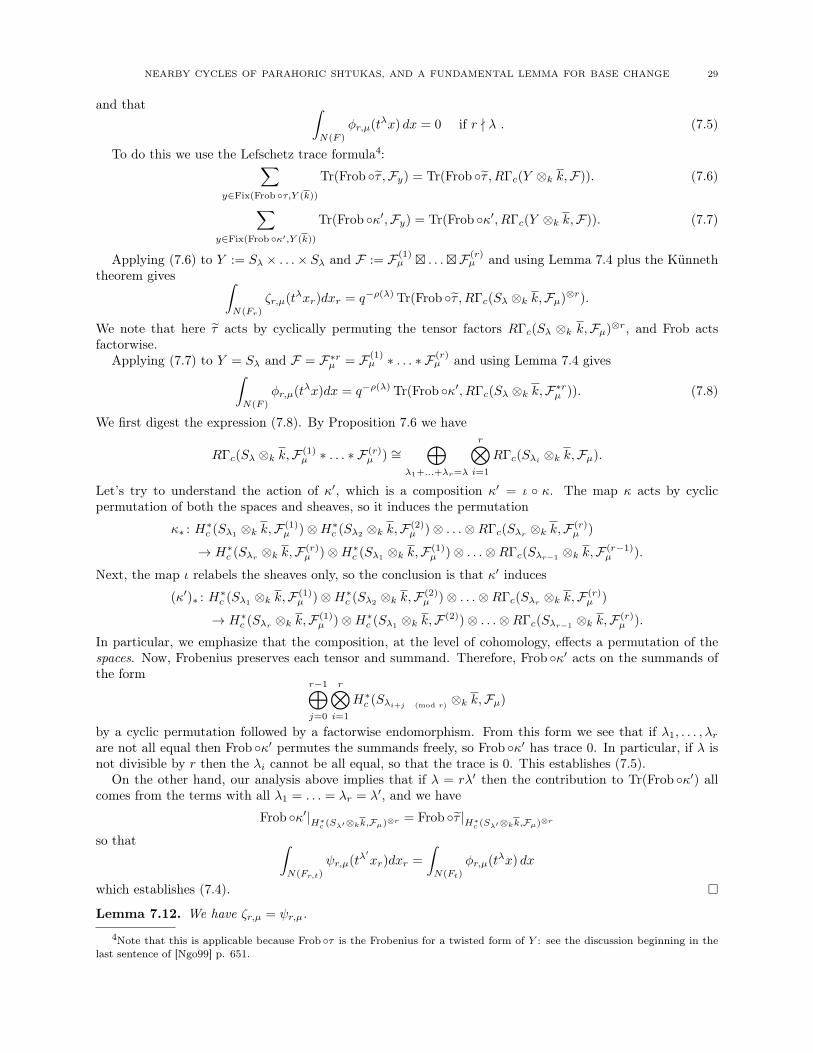
NEARBY CYCLES OF PARAHORIC SHTUKAS, AND A FUNDAMENTAL LEMMA FOR BASE CHANGE 29
and that ∫N(F )
φr,µ(tλx) dx = 0 if r - λ . (7.5)
To do this we use the Lefschetz trace formula4:∑y∈Fix(Frob ◦τ,Y (k))
Tr(Frob ◦τ ,Fy) = Tr(Frob ◦τ , RΓc(Y ⊗k k,F)). (7.6)
∑y∈Fix(Frob ◦κ′,Y (k))
Tr(Frob ◦κ′,Fy) = Tr(Frob ◦κ′, RΓc(Y ⊗k k,F)). (7.7)
Applying (7.6) to Y := Sλ × . . .× Sλ and F := F (1)µ � . . .�F (r)
µ and using Lemma 7.4 plus the Künneththeorem gives ∫
N(Fr)
ζr,µ(tλxr)dxr = q−ρ(λ) Tr(Frob ◦τ , RΓc(Sλ ⊗k k,Fµ)⊗r).
We note that here τ acts by cyclically permuting the tensor factors RΓc(Sλ ⊗k k,Fµ)⊗r, and Frob actsfactorwise.
Applying (7.7) to Y = Sλ and F = F∗rµ = F (1)µ ∗ . . . ∗ F (r)
µ and using Lemma 7.4 gives∫N(F )
φr,µ(tλx)dx = q−ρ(λ) Tr(Frob ◦κ′, RΓc(Sλ ⊗k k,F∗rµ )). (7.8)
We first digest the expression (7.8). By Proposition 7.6 we have
RΓc(Sλ ⊗k k,F (1)µ ∗ . . . ∗ F (r)
µ ) ∼=⊕
λ1+...+λr=λ
r⊗i=1
RΓc(Sλi ⊗k k,Fµ).
Let’s try to understand the action of κ′, which is a composition κ′ = ι ◦ κ. The map κ acts by cyclicpermutation of both the spaces and sheaves, so it induces the permutation
κ∗ : H∗c (Sλ1 ⊗k k,F (1)µ )⊗H∗c (Sλ2 ⊗k k,F (2)
µ )⊗ . . .⊗RΓc(Sλr ⊗k k,F (r)µ )
→ H∗c (Sλr ⊗k k,F (r)µ )⊗H∗c (Sλ1
⊗k k,F (1)µ )⊗ . . .⊗RΓc(Sλr−1
⊗k k,F (r−1)µ ).
Next, the map ι relabels the sheaves only, so the conclusion is that κ′ induces
(κ′)∗ : H∗c (Sλ1⊗k k,F (1)
µ )⊗H∗c (Sλ2⊗k k,F (2)
µ )⊗ . . .⊗RΓc(Sλr ⊗k k,F (r)µ )
→ H∗c (Sλr ⊗k k,F (1)µ )⊗H∗c (Sλ1
⊗k k,F (2))⊗ . . .⊗RΓc(Sλr−1⊗k k,F (r)
µ ).
In particular, we emphasize that the composition, at the level of cohomology, effects a permutation of thespaces. Now, Frobenius preserves each tensor and summand. Therefore, Frob ◦κ′ acts on the summands ofthe form
r−1⊕j=0
r⊗i=1
H∗c (Sλi+j (mod r)⊗k k,Fµ)
by a cyclic permutation followed by a factorwise endomorphism. From this form we see that if λ1, . . . , λrare not all equal then Frob ◦κ′ permutes the summands freely, so Frob ◦κ′ has trace 0. In particular, if λ isnot divisible by r then the λi cannot be all equal, so that the trace is 0. This establishes (7.5).
On the other hand, our analysis above implies that if λ = rλ′ then the contribution to Tr(Frob ◦κ′) allcomes from the terms with all λ1 = . . . = λr = λ′, and we have
Frob ◦κ′|H∗c (Sλ′⊗kk,Fµ)⊗r = Frob ◦τ |H∗c (Sλ′⊗kk,Fµ)⊗r
so that ∫N(Fr,t)
ψr,µ(tλ′xr)dxr =
∫N(Ft)
φr,µ(tλx) dx
which establishes (7.4). �
Lemma 7.12. We have ζr,µ = ψr,µ.
4Note that this is applicable because Frob ◦τ is the Frobenius for a twisted form of Y : see the discussion beginning in thelast sentence of [Ngo99] p. 651.

30 TONY FENG
Proof. By Theorem 7.3 it suffices to check equality of the Satake transforms of both sides. Using Lemma7.4, this amounts to showing
Tr(Frobr, RΓc(Sλ ⊗k k,Fµ)) = Tr(Frob ◦τ , RΓc(Sλ ⊗k k,Fµ)⊗r).
This follows from the general linear algebra fact asserted in Lemma 7.13 below. �
Lemma 7.13 (Saito-Shintani5). Let V be a finite-dimensional representation over a field k. Let τ be theendomorphism of V ⊗r defined by
v1 ⊗ . . .⊗ vr 7→ vr ⊗ v1 ⊗ . . .⊗ vr−1.
Then for all T1, . . . , Tr ∈ End(V ), we have
Tr(T1 . . . Tr, V ) = Tr((T1 ⊗ . . .⊗ Tr)τ, V ⊗r).Proof. If {ei} is a basis for V , then
(T1 ⊗ . . .⊗ Tr)τ(ei1 ⊗ . . .⊗ eir ) = T1(eir )⊗ . . .⊗ Tr(eir−1).
We expand out both sides of the desired equality:
Tr((T1 ⊗ . . .⊗ Tr)τ) =∑
i1,...,ir
〈ei1 ⊗ . . .⊗ eir , T1(eir )⊗ . . .⊗ Tr(eir−1)〉
=∑i1...,ir
〈ei1 , T1(eir )〉 . . . 〈eir , Tr(eir−1)〉
andTr(T1 . . . Tr) =
∑i
〈ei, T1 · · ·Trei〉.
Thus want to show that ∑i1,...,ir
〈ei1 , T1(eir )〉 . . . 〈eir , Tr(eir−1)〉 =∑i
〈ei, T1 · · ·Trei〉.
This follows by repeated iteration of the following more general identity. �
Lemma 7.14. Let V be a finite-dimensional vector space with basis {ei}. For any T ∈ End(V ), we have∑j
〈x, Tej〉〈ej , y〉 = 〈x, Ty〉. (7.9)
Proof. It suffices to establish the equation for y ranging over a basis of V ; taking y = ei the left hand sideis 〈x, Tei〉, and so is the right hand side. �
Combining these results, we obtain the main formula of interest:Theorem 7.15. We have b(ψr,µ) = φr,µ.
Proof. This follows immediately upon combining Proposition 7.11 and Lemma 7.12. �
7.4. Base change for the centers of parahoric Hecke algebras. We now establish an identity forcentral functions of parahoric Hecke algebras analogous to Theorem 7.15. Not surprisingly, this will involveglobalizing to a degeneration from the spherical case.
7.4.1. Setup. We first set some notation. Pick a smooth global curve X/Fq (not necessarily projective) witha rational point x0 ∈ X(Fq). Let G → X be a parahoric group scheme, such that G|X−x0
∼= G × X andG(Ox0
) = J is a parahoric subgroup. We form the affine Grassmannian
π : GrG → X.
Note that for x ∈ X − x0 we haveGrG |x ∼= GrG×kk(x).
For each µ ∈ X∗(T ), we let Fµ := SatGrG (µ) be the (shifted) perverse sheaf on GrG and Fµ,x0 be the re-striction to GrG,x0 . (We have normalized our shifts so that Fµ,x0 is perverse.) We let ψ′r,µ ∈ HG(Fx0⊗FqFqr ),J
be the function as in Definition 5.6.
5We first found this explicitly stated, without proof, in [Ngo06], where it is said to be implicit in the work of Saito andShintani on base change.

NEARBY CYCLES OF PARAHORIC SHTUKAS, AND A FUNDAMENTAL LEMMA FOR BASE CHANGE 31
7.4.2. Convolution product. By Theorem 5.12, RΨ(Fµ) := RΨx0(Fµ) is a central sheaf on GrG,x0 . Wetherefore have, as in Definition 7.10, a map
κ′ : RΨ(Fµ)(1) ∗ . . . ∗RΨ(Fµ)(r)
κ−→ RΨ(Fµ)(r) ∗RΨ(Fµ)(1) ∗ . . . ∗RΨ(Fµ)(r−1)
ι−→ RΨ(Fµ)(1) ∗ . . . ∗RΨ(Fµ)(r).
Definition 7.16. LetRΨ(Fµ)∗r := RΨ(Fµ)(1) ∗ . . . ∗RΨ(Fµ)(r)︸ ︷︷ ︸
r times
.
Define φ′µ : Fix(Frob ◦κ′, RΨ(Fµ)∗r)→ Q` by
φ′µ(y) = Tr(Frob ◦κ′, (RΨ(Fµ)∗r)y).
Theorem 7.17. We have b(ψ′r,µ) = φ′µ.
Proof. By Theorem 5.12, φ′r,µ(y) is in the center of the Iwahori-Hecke algebra. (Since RΨ(Fµ) is central byTheorem 5.12, φ′r,µ(y) clearly commutes with all the other functions of the form φ′r,ν(y); then use that suchthings form a basis for the Iwahori Hecke algebra as ν runs over the extended affine Weyl group.)
Now the argument is essentially the same as for Corollary 5.14. Consider the map
pr: Gr≤µG → Gr≤µG×X
induced by forgetting the level structure at x0. Since pr is proper, by Lemma 5.9 and the fact that pr is anisomorphism away from x0 we have
pr!RΨGrGx0
(Fµ) = RΨGrG×Xx0
(SatGrG×X (µ)).
By Lemma 5.11 and the fact that GrG×X → X is smooth, we have
RΨGrG×Xx0
(SatGrG×X (µ)) ∼= SatGrG×X (µ).
Since pr! corresponds to − ∗J IK at the level functions, this implies
φ′µ ∗J IK = φµ.
Thus by Theorem 7.15 and (7.1), we have that
φ′µ ∗J IK = φµ = b(ψr,µ) = b(ψ′r,µ) ∗J IK . (7.10)
In view of the Bernstein isomorphism (Theorem 5.5), the fact that φ′µ and b(ψ′r,µ) are central plus (7.10)implies that they are equal. �
7.4.3. A global reformulation. We now recast Theorem 7.17 into a form that will be more suitable for oureventual needs.
Let G and GrG be as in §7.4.1. We first recall a construction of the convolution product Fµ ∗ Fµ′ .Recall the iterated global affine Grassmannian GrG,X2 from §4.4.1. We can form the twisted tensor productFµ�Fµ′ := SatGrG,X2 (µ, µ′) on GrG,X2 ([Zhu] §A), which is supported on the Schubert variety Gr
≤(µ,µ′)G,X .
Restricting to the diagonal X ⊂ X2, we have the multiplication map
m : Gr≤(µ,µ′)G,X2 |∆ → Gr≤µ+µ′
G
defined on points by
(x, x, E1ϕ99K E2
β99K E0) 7→ (x, E1
β◦ϕ99K E0).
Then the convolution product is defined by (cf. [MV07] §4 or [Zhu] §5.1)
Fµ ∗ Fµ′ := Rm!(Fµ�Fµ′) ∈ PervL+G(Gr≤µ+µ′
G ). (7.11)

32 TONY FENG
Let us now write down our particular situation of interest. Consider the diagram
Gr≤(µ1,...,µr)G,Xr |∆ ∆(X) ⊂ Xr
Gr≤µ1+...+µrG,X X
m
Then by (7.11) we have
F(µ1) ∗ . . . ∗ F(µr) = Rm!(SatGrG ,Xr (µ1, . . . , µr))
Now Theorem 7.17 can be reformulated as follows, using Corollary 5.9 to commute Rm! and nearby cycles.
Proposition 7.18. Let r.µ := (µ, . . . , µ) ∈ X∗(T )r+. Let fν,x0∈ HG(Fx0
),J be the function fν viewed in theparahoric Hecke algebra of Fx0
, and define ψ′rµ,x0∈ Z(HG(Fx0 ),J) similarly. Then we have
b(ψ′r,rµ,x0) =
∑ν≤rµ
Tr(σ ◦ κ′, RΨXx0
(Rm! SatGr≤r.µG ,Xr
(r.µ))ν)fν,x0 .
8. Comparison of two moduli problems
8.1. Setup. We now let G be the group scheme of units of a global algebra D as in §4.5 and G a parahoricgroup scheme corresponding to some choice of level structure at x0, so ShtG are the D-shtukas studied in§4.5.
Let Z ⊂ X be the set of places of ramification for D. We assume throughout that #Z ≥ n2(||µ1||+ . . .+||µr||), so as to be able to apply Proposition 4.20.
Let X◦ := (X − Z − {x0}). We will now define and compare two different moduli stacks of shtukas.
8.2. Situation A. Let
ShtµA := (Sht≤µG,X /aZ)r.
We have a map
πA : ShtµA |(X−Z)r → (X − Z)r.
By Proposition 4.20 the restriction π◦A := πA|(X◦)r is proper.
Definition 8.1. Let r.µ = (µ, . . . , µ)︸ ︷︷ ︸r times
. We define the following “sheaf” Aµr ∈ Dbc((X
◦)r):
Aµr := Rπ◦A∗(SatShtµA(r.µ)).
We have the following easy but crucial property.
Proposition 8.2. The complex Aµr ∈ is locally constant on (X◦)r, in the sense that each Riπ◦A∗(SatShtµA(r.µ))
is a local system.
Proof. By the properness of π◦A∗ we know that Riπ◦A∗(SatShtµA(r.µ)) is constructible, and the local acyclicity
(Proposition 4.19) then implies that it is locally constant. �
Note that by the Künneth formula, we have
Aµr ∼= (Aµ1 )�r
Choose a basepoint x ∈ X◦, and let xr ∈ (X◦)r denote the diagonal point (x, . . . , x). Then the symmetricgroup Sr acts on (X◦)r, hence also π1((X◦)r, xr). This lifts to an Sr-equivariant structure on the localsystem Aµr , i.e. an action of π1((X◦)r, xr) o Sr on (Aµr )xr , commuting with the action of the global Heckealgebra H⊗r.

NEARBY CYCLES OF PARAHORIC SHTUKAS, AND A FUNDAMENTAL LEMMA FOR BASE CHANGE 33
8.3. Situation B. LetShtµB := Sht≤r.µG,Xr /a
Z
where r.µ = (µ, . . . , µ)︸ ︷︷ ︸r times
. We have a map
πB : ShtµB |(X−Z)r → (X − Z)r.
By the assumption that D is totally ramified at sufficiently many places, the map π◦B := πB |(X◦)r is properby Proposition 4.20.
Definition 8.3. We define the sheaf Bµr on (X◦)r:
Bµr := Rπ◦B∗(SatShtµB(r.µ)).
Proposition 8.4. The complex Bµr ∈ Dbc((X
◦)r) is locally constant on (X◦)r, in the sense that eachRiπ◦B∗(SatShtµB
(r.µ)) is a local system.
Proof. The proof is the same as for Proposition 8.2. �
Again, we have commuting actions of the Hecke algebra H and π1((X◦)r, xr) o Sr on Bµr .
8.4. The comparison theorem.
Theorem 8.5 ([Ngo06]). Let τ ∈ Sr be an r-cycle, i.e. 〈τ〉 ∼= Z/rZ. For g ∈ π1((X◦)r, xr) and h ∈ H wehave
Tr((h⊗ 1 . . .⊗ 1)gτ, (Aµr )xr ) = Tr(hgτ, (Bµr )xr ).
Proof. This is [Ngo06] §3.3 Theorem 1. Since this is really crucial for us, we outline for the sake of expositionhow the proof goes. Keep in mind that Aµr and Bµr are both local systems.
By an application of the Cebotarev density theorem, it suffices to prove the equality for g = Frob(x1,...,xr)
for a dense open subset of Xr, and in particular on the locus (x1, . . . , xr) where the xi are pairwise distinct.On this locus (and under a certain further restriction on the points (x1, . . . , xr)) Ngô independently computesboth sides of the equation, and verifies that they are equal by direct comparison.
Let us say a little more about this computation, which is carried out in [Ngo06] §5. Using the Grothendieck-Lefschetz trace formula to re-express both sides, there are two main inputs: (1) a count of fixed points, and(2) a computation of the trace of Frobenius on the stalks of the relevant sheaves. The counting step isdone as in §6, and the analysis of the stalks enters via results as in §7.3. The interesting feature is that thepairwise distinctness of the points (x1, . . . , xr), plus the extra restriction that we have omitted, turns out toimply that the point counting formulas involve no twisted orbital integrals. Thus, no fundamental lemma isrequired to prove the desired equality.
�
Remark 8.6. For a heuristic that underlies the theorem, coming from a conjectural description of the coho-mology of shtukas, see [Ngo06] §2.2, 3.3. The punchline is that after admitting this conjectural description,the identity in Theorem 8.5 reduces to Lemma 7.13.
Definition 8.7. LetRΨxr0
(Aµr ) := RπA!RΨxr0(SatShtµA
(r.µ)|∆(X◦)) ∈ Dbc(x0)
be the cohomology of nearby cycles at xr0 ∈ ∆(X − Z), and let
RΨxr0(Bµr ) := RπB!RΨxr0
(SatShtµB(r.µ)|∆(X◦)) ∈ Db
c(x0)
be the cohomology of nearby cycles at xr0 ∈ ∆(X − Z).6 Again we apply Remark 5.8 to equip RΨxr0(Aµr )
and RΨxr0(Bµr ) with Fq-structures.
Thanks to Proposition 8.2 and Proposition 8.4, the complex RΨxr0(Aµr ) is equipped with commuting ac-
tions of π1((X◦)r, xr)oSr and (H)⊗r, while RΨxr0(Bµr ) is equipped with commuting actions of π1((X◦)r, xr)o
Sr and H.
Corollary 8.8. For g ∈ π1((X◦)r, xr) and h ∈ H we have
Tr((h⊗ 1 . . .⊗ 1) ◦ Frob ◦τ,RΨxr0(Aµr )) = Tr(h ◦ Frob ◦τ,RΨxr0
(Bµr )). (8.1)
6This is a small abuse of the notation used in §5.2.

34 TONY FENG
Proof. This immediate from Theorem 8.5, Proposition 4.21 plus Corollary 5.10, and the Cebotarev densitytheorem. �
9. Calculation of traces on the cohomology of nearby cycles
Our next step is to combine the work of §5, §6 and §7 to prove Kottwitz-style formulas for both sides of(8.1). We maintain the notation of those preceding sections.
9.1. Calculating the trace in situation A.
Definition 9.1. For a Kottwitz triple (γ0, (γx), (δx)) write
c(γ0, (γx), (δx)) := ker1(F,Gγ0) · vol(J · Jγ0
(F )\Jγ0(AF )) · dg(K)−1
where the notation is as in §6.
Theorem 9.2. Let T ′ ⊂ |X◦|. Assume that Kv := G(Ov) is spherical at all v ∈ T ′. Let
β = (βv ∈ Kv\G(Fv)/Kv)v∈T ′
and hβ ∈ H be the corresponding Hecke operator. Let RΨxr0(Aµr ) be as in Definition 8.7, let τ be as in
Theorem 8.5, let fβv be as in Definition 5.1, and let ψr,µ′ be as in §7.4.1. Then we have
Tr((hβ ⊗ 1 . . .⊗ 1) ◦ Frobx0◦τ,RΨxr0
(Aµr ))
=∑
(γ0,(γx),(δx))inv(γ0,(γx),(δx))=0
c(γ0, (γx), (δx)) ·
∏v 6=x0
Oγv (fβv )
TOδx0σ(ψ′r,µ)
Proof. We’ll use the Lefschetz trace formula to rewrite the trace in terms of a sum of traces over fixed points.The effect of στ on a point of ShtA is illustrated below:
σE1|X−x0
≤µ−−→ E1|X−x0
σE2|X−x0
≤µ−−→ E2|X−x0
...σEr|X−x0
≤µ−−→ Er|X−x0
στ−−→
σ2Er|X−x0
≤µ−−→ σEr|X−x0
σ2E1|X−x0
≤µ−−→ σE1|X−x0
...σ2Er−1|X−x0
≤µ−−→ σEr−1|X−x0.
.
Therefore, a fixed point of the correspondence (hβ ⊗ 1 . . . ⊗ 1) ◦ Frobx0◦τ corresponds to a point as above
such that
E2 = σE1...Er = σEr−1
E1=β−−→ σEr.
Hence a fixed point is equivalent to the data of commuting modifications
t : σE1|X−x0
≤µ−−→ E1|X−x0
t′ : σr
E1|X−T ′=β−−→ E1|X−T ′ .
Hence in the notation of §6 we see that
Fix((hβ ⊗ 1 . . .⊗ 1) ◦ Frobx0 ◦τ) =⋃ν≤µ
C(νx0 , β;x0, T′; r).
By Lemma 5.9 plus Proposition 4.21, we have
RΨxr0(Aµr ) ∼= RπA!(RΨxr0
(SatShtA(r.µ))).
NEARBY CYCLES OF PARAHORIC SHTUKAS, AND A FUNDAMENTAL LEMMA FOR BASE CHANGE 35
Now invoking the Grothendieck-Lefschetz trace formula, we have
Tr((hβ ⊗ 1 . . .⊗ 1) ◦ Frobx0◦τ,RΨxr0
(Aµr ))
=∑ν≤µ
∑Ξ∈C(νx0
,β;x0,T ′;r)
Tr((hβ ⊗ 1 . . .⊗ 1) ◦ Frob ◦τ,RΨxr0(SatShtA(r.µ))Ξ).
By Corollary 5.22, for all Ξ ∈ C(νx0, β;x0, T
′; r) we have
RΨxr0(SatShtA(r.µ))Ξ = RΨxr0
(SatGrrG(r.µ))ν .
Now using Corollary 6.14, we can rewrite our formula as
Tr((hβ ⊗ 1 . . .⊗ 1) ◦ Frobx0 ◦τ,RΨxr0(Aµr ))
=∑
(γ0,(γx),(δx))inv(γ0,(γx),(δx))=0
c(γ0, (γx), (δx)) ·∏v 6=x0
Oγv (fβv )
·∑ν≤µ
TOδx0σ(fν) · Tr((hβ ⊗ 1 . . .⊗ 1) ◦ Frob ◦τ,RΨxr0
(SatGrrG(r.µ))ν). (9.1)
Since the Hecke operator hβ supports a modification at T ′, which is disjoint from x0, it acts trivially on allthe stalks lying over xr0, so we may ignore it when computing the trace in (9.1). Since
RΨxr0(SatGrrG
(r.µ)) ∼= RΨx0(SatGrG (µ))�r, (9.2)
the trace of Frob ◦τ coincides with the trace of Frobenius for the Satake sheaf on the Weil restrictionReskr/k(Gr≤µG ⊗FqFqr ). Therefore, by [Ngo06] §5.2 Proposition 3, we have7
Tr(Frob ◦τ,RΨxr0(SatGrrG
(r.µ))ν) = Tr(Frobr, RΨxr0(SatGrG (µ))ν). (9.3)
Substituting (9.3) into (9.1) we arrive at
Tr((hβ ⊗ 1 . . .⊗ 1) ◦ Frobx0◦τ,RΨxr0
(Aµr ))
=∑
(γ0,(γx),(δx))inv(γ0,(γx),(δx))=0
c(γ0, (γx), (δx)) ·∏v 6=x0
Oγv (fβv )
·∑ν≤µ
TOδx0σ(fν) · Tr(Frobr, RΨxr0
(SatGrG (µ))ν). (9.4)
By Lemma 5.17 we have the following identity:
ψ′r,µ =∑ν≤µ
Tr(Frobr, RΨxr0(SatGrG (µ))ν)fν .
Substituting this in (9.4), we finally find
Tr((hβ ⊗ 1 . . .⊗ 1) ◦ Frobx0 ◦τ,RΨxr0(Aµr ))
=∑
(γ0,(γx),(δx0))
inv(γ0,(γx),(δx))=0
c(γ0, (γx), (δx)) ·
∏v 6=x0
Oγv (fβv )
· TOδx0σ(ψ′r,µ)
which is what we wanted to show. �
7The proof of this formula, which is not explicitly written in [Ngo06], goes as follows. By (9.2) we have
Tr(Frob ◦τ, RΨxr0 (SatGrrG(r.µ))ν) = Tr(Frob ◦τ, RΨx0 (SatGrG (µ))�rν )
= Tr(Frobr, RΨx0 (SatGrG (µ))ν),
where in the last equality we used Lemma 7.13.

36 TONY FENG
9.2. Calculating the trace in situation B. We now want to prove an analogous formula for the trace insituation B. The computation in this case is a little more involved. The main reason is that the action of Sron Bxr0 is difficult to understand explicitly. Recall that is was obtained from the fact that B|U was a localsystem, so that we could extend it over X. However, this process obfuscates the geometric meaning of thisaction, and we will need to use the results of §7, particularly the geometric model of base change studied in§7.4.3, in order to understand it.
Theorem 9.3. Let T ′ ⊂ |X◦|. Assume that Kv := G(Ov) is spherical at all v ∈ T ′. Let
β = (βv ∈ Kv\G(Fv)/Kv)v∈T ′
and hβ ∈ H be the corresponding Hecke operator. Let RΨxr0(Bµr ) be as in Definition 8.7, let τ be as in
Theorem 8.5, and let ψr,µ′ be as in §7.4.1. Then we have
Tr(hβ ◦ Frobx0 ◦τ,RΨxr0(Bµr ))
=∑
(γ0,(γx),(δx))inv(γ0,(γx),(δx))=0
c(γ0, (γx), (δx)) ·
∏v 6=x0
Oγv (fβv )
·Oγx0(b(ψ′r,µ)).
Proof. Let X(r) = Symr(X) by the rth symmetric power of X, and
ShtµB,X(r) := Sht≤r.µG,X(r) /a
Z.
The idea here is to push down the computation from Xr to X(r), which trivializes the Sr action on the fiberShtB,X(r) over a point, transferring the effect of this action completely to the sheaf theory, where it wasstudied in §7. Consider the following commutative diagram, in which the front cartesian square is the fiberof the back cartesian square over the diagonal copy of X in X(r).
ShtµB Xr
ShtµB,X(r) X(r)
Sht≤r.µB |∆ ∆(X)
Sht≤rµG,X /aZ ∆(X)
m add
m add
π
(9.5)
The map add: Xr → X(r) is totally ramified over the diagonal ∆(X) ⊂ Xr, so for any étale sheaf F on Xr
the stalk of F at xr ∈ Xr is canonically identified with the stalk of add∗F at add(xr) ∈ X(r). Therefore,from the front cartesian square we have
Tr(hβ ◦ Frobx0◦τ,RΨxr0
(Bµr )) = Tr(hβ ◦ Frobx0◦τ,RΨxr0
(Rπ◦! Rm! SatShtµB(r.µ)))
where π◦ is the restriction of π to the fiber over (the diagonal embedding of) X◦. We now proceeding asbefore, using the Grothendieck-Lefschetz trace formula to rewrite the trace in terms of a sum of traces overfixed points. We begin by describing the fixed points of hβ ◦ Frobx0
◦τ on Sht≤rµG,X /aZ.Now, on Shtµ
B,X(r) the permutation τ evidently acts trivially. A point of ShtG,X /aZ|x0
is a modification
σE1|X−x0
≤rµ−−−→ E1|X−x0
occurring over x0. The map σ takes this to
σ2
E1|X−x0
≤rµ−−−→ σE1|X−x0.

NEARBY CYCLES OF PARAHORIC SHTUKAS, AND A FUNDAMENTAL LEMMA FOR BASE CHANGE 37
Therefore, a fixed point of the correspondence hβ ◦ Frobx0 ◦τ is equivalent to the data of commuting modi-fications
t : σE1|X−x0
≤rµ−−−→ E1|X−x0
t′ : σE1|X−T ′=β−−→ E1|X−T ′ .
Hence we see that (remember that x0 is assumed to have degree 1)
Fix(hβ ◦ Frobx0 ◦τ) =⋃ν≤rµ
C(νx0 , β;x0, T′; 1)
so by the Grothendieck-Lefschetz trace and arguing as in §9.1 for situation A,
Tr(hβ ◦ Frobx0◦τ,RΨxr0
(Bµr )) =∑ν≤rµ
#C(νx0, β;x0, T
′; 1)
· Tr(hβ ◦ Frob ◦τ,RΨxr0(Rm! SatShtµB
(r.µ))ν).
Using Theorem 6.14, we rewrite this as
Tr(hβ ◦ Frobx0◦τ,RΨxr0
(Bµr ))
=∑
(γ0,(γx),(δx))inv(γ0,(γx),(δx))=0
c(γ0, (γx), (δx)) ·∏v 6=x0
Oγv (fβv )
·∑ν≤µ
TOδx0(fν) · Tr(hβ ◦ Frob ◦τ,RΨxr0
(Rm! SatShtµB(r.µ))ν). (9.6)
As in the previous calculation for situation A, the Hecke operator acts trivially on the stalk at x0 becauseis supported on a disjoint set of points. We use the affine Grassmannian as a local model to calculateTr(Frobx0
◦τ,RΨxr0(Rm!SatShtB (r.µ))ν). By Theorem 5.19, we have
Tr(Frobx0◦τ,RΨxr0
(Rm! SatShtµB(r.µ))ν) = Tr(Frobx0
◦κ′, RΨxr0(Rm! Sat
Gr≤r.µG,Xr
(r.µ))ν), (9.7)
where the notation on the right hand side is as in Corollary 7.18, if we can show that the permutation τ onthe left side is carried by Theorem 5.19 to the permutation κ′ studied in §7.4.3. (The same issue is raisedand explained in [Ngo06] §5.6 Proposition 3.) To prove it, consider the diagram
W≤r.µXr
Gr≤r.µG,Xr W≤rµX(r) ShtµB Xr
Gr≤rµG,X(r) ShtµB,X(r) X(r)
étalem
m étale m add
Here W≤r.µXr expresses Gr≤r.µG,Xr as a local model for Sht≤r.µB |∆ and W≤rµX(r) expresses Gr≤rµG,X(r) as a local model
for ShtµB,X(r) . The existence of such a commutive diagram is immediate from the proof of Theorem 5.19.
The claim is then that the permutation actions on RΨxr0(Rm! SatGrG,Xr (r.µ)) and RΨxr0
(Rm!SatShtB (r.µ)),induced by middle extension from (X◦)r to (X − Z)r, are compatible. This is clear from the diagram andthe fact that the identity can be checked on the locus where the points (x1, . . . , xr) are distinct, where it isevidently given by the same geometric permutation action in both cases.
Now combining Proposition 7.18, Corollary 5.22, and Lemma 5.17, we have
b(ψ′r,µ) =∑ν≤rµ
Tr(Frob ◦κ′, RΨxr0(Rm! SatGrG (µ))ν)fν . (9.8)

38 TONY FENG
Putting together (9.6), (9.7), and (9.8) gives
Tr((hβ ⊗ 1 . . .⊗ 1) ◦ Frobx0 ◦τ,RΨxr0(Bµr ))
=∑
(γ0,(γx),(δx0))
inv(γ0,(γx),(δx))=0
c(γ0, (γx), (δx)) ·
∏v 6=x0
Oγv (fβv )
TOδx0(b(ψ′r,µ))
which is what we wanted to show. �
9.3. The base change fundamental lemma for parahoric Hecke algebras. We can now deduce somecases of the base change fundamental lemma.
Corollary 9.4. Let T ′ ⊂ |X◦|. Assume that Kv := G(Ov) is spherical at all v ∈ T ′. Let
β = (βv ∈ Kv\G(Fv)/Kv)v∈T ′
and hβ ∈ H be the corresponding Hecke operator. Let ψr,µ′ be as in §7.4.1 and the base change homomorphimψr,µ′ 7→ b(ψr,µ′) be as in §7.1. Then we have
∑(γ0,(γx),(δx))
inv(γ0,(γx),(δx))=0
c(γ0, (γx), (δx)) ·
∏v 6=x0
Oγ0(fβv )
· TOδx0σ(ψ′r,µ)
=∑
(γ0,(γx),(δx0))
inv(γ0,(γx),(δx))=0
c(γ0, (γx), (δx)) ·
∏v 6=x0
Oγ0(fβv )
·Oγ0(b(ψ′r,µ))
Proof. This follows immediately from substituting Theorem 9.2 and Theorem 9.3 into Corollary 8.8, and thefollowing comment about changing the γv to γ0: since by definition of X−Z we have that G(Fx) ∼= GLn(Fx)for all x ∈ X − Z, the notion of stable conjugacy coincides with the notion of conjugacy. �
It seems to be “well-known” how to deduce a fundamental lemma from a statement such as Corollary 9.4.8
Nevertheless, let us give a proof for completeness, following [Ngo06] §5.7 Théorème 1. First we introduce apiece of notation.
Definition 9.5. For µ = (µ1, . . . , µn) ∈ X∗(GLn) ∼= Zn, we define
|µ| := µ1 + . . .+ µn.
The stack Sht≤µG is non-empty if and only if |µ| = 0, because a G-bundle has the notion of degree on X,which is preserved by the Frobenius twist σ on S. Let
Z(HG(Fx0,r),J)0 ⊂ Z(HG(Fx0 ),J)
be the subspace generated by the ψ′r,µ with |µ| = 0, which is the same as the subspace generated by the ψr,µwith |µ| = 0.
Theorem 9.6. Let Fx0be a local field of characteristic p, and Fx0,r/Fx0
the unramified extension of degreer. Let δ be a σ-conjugacy class in GLn(Fx0,r), with norm Nδx0 = γx0 ∈ GLn(Fx0). Assume γx0 is regularsemisimple and separable. If φ ∈ Z(HG(Fx0,r),J)0, then we have
TOδx0σ(φ) = Oγx0
(b(φ)).
Proof. Choose a global curve X with function field F , and write Fx0∼= Fq((t)). Choose a division algebra
D as in §8.1, and define G and G as in §4.5. We can then apply Corollary 9.4.For a fixed function h ∈ HG,K(A) the orbital integrals and twisted orbital integrals are locally constant
near regular semisimple separable elements. Therefore, by weak approximation we can choose γ ∈ G(F )
8It is remarked on p.84 of the Arxiv version 2 of [Ngo06] that this is “standard”, and a reference is given to [Clo90].

NEARBY CYCLES OF PARAHORIC SHTUKAS, AND A FUNDAMENTAL LEMMA FOR BASE CHANGE 39
close enough to γt in the t-adic topology so that γ = N(δx0) ∈ G(Ft⊗Fq Fqr ) for some δx0 ∈ G(Ft⊗Fq Fqr ),and such that
Oγx0(b(ψµ)) = Oγ(b(ψµ))
TOδx0σx0
(ψµ) = TOδx0σx0
(ψµ).
We can choose an appropriate Hecke operator h = (hv) ∈ HG(A) so that Oγ(hv) 6= 0 for v 6= x.Because a fixed choice of h is the identity at all but finitely many places, any Kottwitz triple for which
the product of orbital integrals is non-zero forces the γv to be in Kv at all but finitely many v. Then by[Kot86b] Proposition 7.1 there are only finitely many possibilities for the Kottwitz triple, as all γv outside afixed finite set must be (rationally) conjugate to γ. (Technically this discussion is unnecessary here becausewe are only dealing with GLn at this point.) Therefore, since the support of any adelic Hecke operator iscompact open in G(A), while G(F ) is discrete, for any fixed h ∈ HG,K(A) there are only finitely manynon-zero summands in Corollary 9.4.
Again by the discreteness of G(F ) in G(A), we may shrink the support of the chosen Hecke operatorappropriately so that all the terms∏
v 6=x0
Oγ0(hv)
· TOδx0σ(ψ′r,µ) and
∏v 6=x0
Oγ0(hv)
·Oγ0(b(ψ′r,µ))
vanish except for the chosen γx0 . Then we have
c(γ0, (γx), (δx)) ·
∏v 6=x0
Oγ0(hv)
· TOδx0σ(ψ′r,µ)
= c(γ0, (γx), (δx)) ·
∏v 6=x0
Oγ0(hv)
·Oγ0(b(ψ′r,µ))
Since |µ| = 0, Sht≤µG is non-empty so these terms are not 0. Dividing out by the common (necessarily
non-zero) factor c(γ0, (γx), (δx)) ·(∏
v 6=x0Oγ0
(hv))then yields the desired equality for all ψ′r,µ with |µ| = 0.
We conclude by observing that these span Z(HG(Fx0,r),J)0. �
References
[Bro13] Michael Broshi, G-torsors over a Dedekind scheme, J. Pure Appl. Algebra 217 (2013), no. 1, 11–19. MR 2965898[Clo90] Laurent Clozel, The fundamental lemma for stable base change, Duke Math. J. 61 (1990), no. 1, 255–302. MR 1068388[Del73] P. Deligne, Séminaire de géométrie algébrique du Bois Marie: Groupes de Monodromie en Géometrie Algébrique
(SGA 7 II)., Lecture Notes in Mathematics, vol. 569, Springer-Verlag, 1973.[Dri87] V. G. Drinfel’d, Cohomology of compactified moduli varieties of F -sheaves of rank 2, Zap. Nauchn. Sem. Leningrad.
Otdel. Mat. Inst. Steklov. (LOMI) 162 (1987), no. Avtomorfn. Funkts. i Teor. Chisel. III, 107–158, 189. MR 918745[Gai01] D. Gaitsgory, Construction of central elements in the affine Hecke algebra via nearby cycles, Invent. Math. 144
(2001), no. 2, 253–280. MR 1826370[Gro98] Benedict H. Gross, On the Satake isomorphism, Galois representations in arithmetic algebraic geometry (Durham,
1996), London Math. Soc. Lecture Note Ser., vol. 254, Cambridge Univ. Press, Cambridge, 1998, pp. 223–237.MR 1696481
[Hai09] Thomas J. Haines, The base change fundamental lemma for central elements in parahoric Hecke algebras, Duke Math.J. 149 (2009), no. 3, 569–643. MR 2553880
[HRa] Thomas Haines and Timo Richarz, The test function conjecture for parahoric local models, Preprint available athttps://arxiv.org/pdf/1801.07094.pdf.
[HRb] Urs Hartl and Esmail Arasteh Rad, Langlands-rapoport conjecture over function fields, Preprint available at https://arxiv.org/pdf/1605.01575.pdf.
[Kot80] Robert Edward Kottwitz, Orbital integrals on GL3, Amer. J. Math. 102 (1980), no. 2, 327–384. MR 564478[Kot86a] Robert E. Kottwitz, Base change for unit elements of Hecke algebras, Compositio Math. 60 (1986), no. 2, 237–250.
MR 868140[Kot86b] , Stable trace formula: elliptic singular terms, Math. Ann. 275 (1986), no. 3, 365–399. MR 858284[Kot90] , Shimura varieties and λ-adic representations, Automorphic forms, Shimura varieties, and L-functions, Vol.
I (Ann Arbor, MI, 1988), Perspect. Math., vol. 10, Academic Press, Boston, MA, 1990, pp. 161–209. MR 1044820[Kot92] , Points on some Shimura varieties over finite fields, J. Amer. Math. Soc. 5 (1992), no. 2, 373–444. MR 1124982

40 TONY FENG
[KP] Mark Kisin and Georgios Pappas, Integral models of Shimura varieties with parahoric level structure, Preprint avail-able at https://arxiv.org/pdf/1512.01149.pdf.
[KW01] Reinhardt Kiehl and Rainer Weissauer, Weil conjectures, perverse sheaves and l’adic Fourier transform, Ergebnisseder Mathematik und ihrer Grenzgebiete. 3. Folge. A Series of Modern Surveys in Mathematics [Results in Mathematicsand Related Areas. 3rd Series. A Series of Modern Surveys in Mathematics], vol. 42, Springer-Verlag, Berlin, 2001.MR 1855066
[Lab90] J.-P. Labesse, Fonctions élémentaires et lemme fondamental pour le changement de base stable, Duke Math. J. 61(1990), no. 2, 519–530. MR 1074306
[Laf97] Laurent Lafforgue, Chtoucas de Drinfeld et conjecture de Ramanujan-Petersson, Astérisque (1997), no. 243, ii+329.MR 1600006
[Laf02] , Chtoucas de Drinfeld et correspondance de Langlands, Invent. Math. 147 (2002), no. 1, 1–241. MR 1875184[Laf12] Vincent Lafforgue, Chtoucas pour les groupes réductifs et paramétrisation de Langlands globale, preprint,
https://arxiv.org/pdf/1209.5352.pdf (2012).[Lau04] Eike Sören Lau, On generalised D-shtukas, Bonner Mathematische Schriften [Bonn Mathematical Publications], vol.
369, Universität Bonn, Mathematisches Institut, Bonn, 2004, Dissertation, Rheinische Friedrich-Wilhelms-UniversitätBonn, Bonn, 2004. MR 2206061
[MV07] I. Mirković and K. Vilonen, Geometric Langlands duality and representations of algebraic groups over commutativerings, Ann. of Math. (2) 166 (2007), no. 1, 95–143. MR 2342692
[ND13] Tuan Ngo Dac, Comptage des G-chtoucas: la partie elliptique, Compos. Math. 149 (2013), no. 12, 2169–2183.MR 3143709
[ND15] , On a counting problem for G-shtukas, Arithmetic and geometry, London Math. Soc. Lecture Note Ser., vol.420, Cambridge Univ. Press, Cambridge, 2015, pp. 318–350. MR 3467129
[Ngo99] Bao Châu Ngo, Faisceaux pervers, homomorphisme de changement de base et lemme fondamental de Jacquet et Ye,Ann. Sci. École Norm. Sup. (4) 32 (1999), no. 5, 619–679. MR 1710755
[Ngo06] , D-chtoucas de Drinfeld à modifications symétriques et identité de changement de base, Ann. Sci. École Norm.Sup. (4) 39 (2006), no. 2, 197–243. MR 2245532
[NND08] Bao Châu Ngô and Tuân Ngô Dac, Comptage de G-chtoucas: la partie régulière elliptique, J. Inst. Math. Jussieu 7(2008), no. 1, 181–203. MR 2398149
[PR10] Georgios Pappas and Michael Rapoport, Some questions about G-bundles on curves, Algebraic and arithmetic struc-tures of moduli spaces (Sapporo 2007), Adv. Stud. Pure Math., vol. 58, Math. Soc. Japan, Tokyo, 2010, pp. 159–171.MR 2676160
[PZ13] G. Pappas and X. Zhu, Local models of Shimura varieties and a conjecture of Kottwitz, Invent. Math. 194 (2013),no. 1, 147–254. MR 3103258
[RD] Walter Randolph Ray-Dulany, Base change for the iwahori-hecke algebra of gl2, Ph.D. thesis. Available at https://drum.lib.umd.edu/bitstream/handle/1903/10963/RayDulany_umd_0117E_11632.pdf?sequence=1&isAllowed=y.
[Ric16] Timo Richarz, Affine Grassmannians and geometric Satake equivalences, Int. Math. Res. Not. IMRN (2016), no. 12,3717–3767. MR 3544618
[Var04] Yakov Varshavsky, Moduli spaces of principal F -bundles, Selecta Math. (N.S.) 10 (2004), no. 1, 131–166. MR 2061225[Zhu] Xinwen Zhu, An introduction to affine Grassmannians and the geometric Satake equivalence, To appear in Proceedings
of the IAS/Park City Mathematics Series. Preprint available at https://arxiv.org/pdf/1603.05593.pdf.[Zhu14] , On the coherence conjecture of Pappas and Rapoport, Ann. of Math. (2) 180 (2014), no. 1, 1–85. MR 3194811