University of Texas at El Paso University of Texas at El Paso

ScholarWorks@UTEP ScholarWorks@UTEP

Open Access Theses & Dissertations

2019-01-01

Near Room Temperature Magnetocaloric Materials for Magnetic Near Room Temperature Magnetocaloric Materials for Magnetic

Refrigeration Refrigeration

Eduardo Martinez Teran University of Texas at El Paso

Follow this and additional works at: https://digitalcommons.utep.edu/open_etd

Part of the Environmental Sciences Commons, and the Physics Commons

Recommended Citation Recommended Citation Martinez Teran, Eduardo, "Near Room Temperature Magnetocaloric Materials for Magnetic Refrigeration" (2019). Open Access Theses & Dissertations. 2914. https://digitalcommons.utep.edu/open_etd/2914

This is brought to you for free and open access by ScholarWorks@UTEP. It has been accepted for inclusion in Open Access Theses & Dissertations by an authorized administrator of ScholarWorks@UTEP. For more information, please contact lweber@utep.edu.

NEAR ROOM TEMPERATURE MAGNETOCALORIC MATERIALS

FOR MAGNETIC REFRIGERATION

EDUARDO MARTÍNEZ TERÁN

Master’s Program in Physics

APPROVED:

Ahmed El-Gendy, Ph.D., Chair

Rajendra Zope, Ph.D.

Deidra R. Hodges, Ph.D.

Stephen L. Crites, Jr., Ph.D.

Dean of the Graduate School

Copyright ©

by

Eduardo Martínez Terán

2019

Dedication

I dedicate this work to my parents, who’ve constantly supported my academic and life decisions.

NEAR ROOM TEMPERATUREMAGNETOCALORIC EFFECT FOR

MAGNETIC REFRIGERATION

by

EDUARDO MARTÍNEZ TERÁN, B.S.

THESIS

Presented to the Faculty of the Graduate School of

The University of Texas at El Paso

in Partial Fulfillment

of the Requirements

for the Degree of

MASTER OF SCIENCE

Department of Physics

THE UNIVERSITY OF TEXAS AT EL PASO

December 2019

v

Acknowledgements

I would like to express gratitude to my advisor Dr. Ahmed El-Gendy, who gave me the opportunity

to join his research group and helped and encouraged me without hesitation during my research

learning.

vi

Table of Contents

Acknowledgements ..........................................................................................................................v

Table of Contents ........................................................................................................................... vi

List of Tables ................................................................................................................................ vii

List of Figures .............................................................................................................................. viii

Chapter 1: Introduction ...................................................................................................................1

1.1 General Overview of the Magnetocaloric Effect ..............................................................1

1.2 Thermodynamics of the Magnetocaloric Effect ...............................................................2

1.2.1 Magnetic Phase Transitions and Magnetocaloric Materials Classification .........8

1.2.2 Magnetocaloric Effect and Thermodynamic Cycles ...........................................11

1.2.3 Requirements for a Good Magnetocaloric Material ...........................................13

1.3 Heusler Alloy System .....................................................................................................14

Chapter 2: Experimental Methods .................................................................................................18

2.1 Sample Preparation .........................................................................................................18

2.1.1 Arc Melting and Melt Spin .................................................................................18

2.2 Sample Characterization .................................................................................................19

2.2.1 X-Ray Diffraction ...............................................................................................20

2.2.2 Vibrating Sample Magnetometer ........................................................................20

2.3 Magnetic Measurements for Magnetocaloric Effect .......................................................22

2.3.1 Direct Method .....................................................................................................22

2.2.1 Indirec Method ....................................................................................................23

Chapter 3: Magnetic and Magnetocaloric Properties of MnFe2Ga Alloy ......................................26

3..1 Introduction ....................................................................................................................26

3..1 Experimental Details ......................................................................................................26

3..1 Results and Discussion ..................................................................................................27

3..1 Conslusion......................................................................................................................32

References ......................................................................................................................................34

Vita .................................................................................................................................................37

vii

List of Tables

Table 3.1: Transition temperature T1, change in entropy and relative cooling power at the near

room temperature. .................................................................................................................31

Table 3.2: Curie transition temperature Tc, change in entropy and relative cooling power at

the high temperature ............................................................................................................32

viii

List of Figures

Figure 1.1: The total entropy S as a function of magnetic field H and temperature T,

schematically illustrating the definition of the isothermal magnetic entropy change ΔSM and

the adiabatic temperature change ΔTad ............................................................................................7

Figure 1.2: Magnetization M, heat capacity Cp, entropy S and entropy change dependence on

the field change at first and second order transitions ...........................................................10

Figure 1.3: Comparison between a conventional vapor compressor refrigerator and a magnetic

refrigerator ...........................................................................................................................11

Figure 1.4: T-S diagram of an MR (a) Carnot cycle; (b) Bryton cycle; (c) Ericsson cycle ...........12

Figure 1.5: Definitions of relative cooling power (RCP) and refrigerant capacity (RC) for

GdRu0.2Cd0.8. The rectangular area is RCP and the area full with parallel lines is RC ........14

Figure 1.6: C1b and L21 structures adapted by the half- and full-Heusler alloys ...........................15

Figure 1.7: Possible configurations in the B2 disordered structure given by the occupation of

Y and Z sublattices for Heusler alloys ..................................................................................16

Figure 1.8: Stress-Temperature graph and Stress-Strain graph of martensite to austenite lines

in a shape memory alloy .......................................................................................................17

Figure 2.1: Components of the Arc Melting Furnace SA-200-1-VM ..........................................18

Figure 2.2: Basic configuration of a single-roller melt-spinning apparatus ..................................19

Figure 2.3: Diffraction (i.e. constructive interference of the scattered X-rays) will occur if the

Bragg condition (eq. 1) is fulfilled and of the scattering vector K is parallel to the normal

of the hkl-planes ....................................................................................................................20

Figure 2.4: Schematic representation of a Vibrating sample Magnetometer (VSM) ....................22

Figure 2.5: Adiabatic temperature change during a magnetic field change of 1.1 T for a test

sample of Gd 99.9 % .............................................................................................................23

Figure 2.6: Experimentally observed magnetization M in melt-spun LaFe11.6Si1.4 showing a

weak first order transition in dependence on (a) temperature and (b) magnetic field ..........23

Figure 2.7: Process for calculating the magnetic change in entropy with the indirect method.

(a) Magnetic isotherms are measured. (b-c) Entropy at each temperature is calculated. (d)

Difference of magnetic entropy is obtained ..........................................................................24

Figure 3.1: X-ray diffraction pattern of samples at room temperature ..........................................27

Figure 3.2: Magnetization dependence on temperature at a constant field of 100 Oe ..................28

Figure 3.3: Differential scanning calorimetry measurements for the annealed ribbons, showing

the low, Martensitic and Curie transition temperatures ........................................................29

Figure 3.4: Hysteresis loop of the ribbon annealed for two hours, at different temperatures in

intervals of 5 K. (a) From 50 to 400 K and (b) from 300 to 800K. ......................................30

Figure 3.5: Arrot plots around phase transition temperatures, showing a first order transition at

320K and a first order transition at 550K .............................................................................30

Figure 3.3: Change in entropy for all the ribbon samples at a 0-3T external field strenght .........31

1

Chapter 1: Introduction

In today’s society, cooling technology has become a necessity, whereas for food transport

and storage, allowing us to have off seasonal products; for our commodity, with air conditioning

in our homes and cars; for medical advances, such as organ transplantation or cryogenic storage.

The modern refrigerator/cooling system operational design has not changed much in comparison

with their earliest design versions, they operate via a gas expansion and compression cycle that

uses chemicals such as Freon, a refrigerant which is an ozone depleting compound that consists of

chlorofluorocarbons (CFCs) and hydrochlorofluorocarbons (HCFCs). The implementation of

new designs and materials for the construction of cooling systems is a must do, being essential that

these improved designs will reduce the environmental impact and increase the efficiency of their

predecessors.

General Overview of Magnetocaloric Effect

Magnetic refrigeration (MR) is a cooling process based on the magnetocaloric effect (MCE) that

is present to some extent in all magnetic materials, and the ones in which this effect is more

appreciable are called magnetocaloric materials (MCM) [1]. MR has been an emerging technology

for the last 20 years and the interest shown by researchers, industry and governmental agencies [2]

promises a non-so distant future where MCM’s will be implemented at a faster rate than today’s

conventional refrigerative systems. This new cooling technology is projected to have a 20% in

energy savings for A/C applications and 40-50% in savings for refrigeration applications [3].

Although a liquid is still needed as a heat exchanger, various designs for the arrangement of

magnetocaloric materials for magnetic refrigeration have been proposed, such as a rotatory device

[4] and a fully solid-state magnetic refrigerator [5].

2

Before being implemented in MR at room temperature, any MCM should met few criteria:

• It’s Curie temperature (TC) should be around room temperature.

• Reversible magnetization process with respect to a changing and reversing external

magnetic field.

• Small hysteresis loss in the magnetization/demagnetization process.

• Nontoxic and oxidation resistant.

• Low cost magnetic materials and processing.

Thermodynamics of Magnetocaloric Effect

The theory of the MCE surfaces by considering the MCM as a thermodynamic system and

applying the first law of thermodynamics. The total internal energy of the system can be described

as function of the external magnetic field (𝐻), the volume (𝑉) and entropy (𝑆) of the system

𝑈 = 𝑈(𝑆, 𝑉, 𝐻) ( 1.1)

and can also be written as a function of the magnetic moment (𝑀), 𝑉 and 𝑆:

𝑈 = 𝑈(𝑆, 𝑉, 𝑀) (1. 2)

For each of the representations of the internal energy (𝑈), the total derivative takes the following

corresponding forms

𝑑𝑈 = 𝑇𝑑𝑆 − 𝑃𝑑𝑉 + 𝑀𝑑𝐻 (1. 3a)

𝑑𝑈 = 𝑇𝑑𝑆 − 𝑃𝑑𝑉 + 𝐻𝑑𝑀 (1. 3b)

3

Considering that there will be no volume change (𝑑𝑉 = 0), and normalizing the magnetization by

the mass of the sample (𝜎 – magnetic moment per unit of mass) we end up with the relations for

the internal energy

𝑑𝑈 = 𝑇𝑑𝑆 + 𝐻𝑑𝑀 → 𝑑𝑈 = 𝑇𝑑𝑆 + 𝐻𝑑𝜎 (1. 4a)

𝑑𝑈 = 𝑇𝑑𝑆 + 𝑀𝑑𝐻 → 𝑑𝑈 = 𝑇𝑑𝑆 + 𝜎𝑑𝐻 (1. 4b)

From this expression we can see that now the entropy of the system can be described in terms of

the variables corresponding to the temperature of the system 𝑇 and the external applied magnetic

field 𝐻

𝑆 = 𝑆(𝐻, 𝑇) (1.5)

Taking the derivative of the entropy 𝑆 = 𝑆(𝐻, 𝑇)

𝑑𝑆 = (𝜕𝑆 𝜕𝑇⁄ )𝐻𝑑𝑇 + (𝜕𝑆 𝜕𝐻⁄ )𝑇𝑑𝐻 (1.6)

it’s observable that the total change in Entropy of the system will have two contributions, one is

related to the change in the temperature of the system at constant H and the other one to the change

in the magnetic field at constant temperature 𝑇.

For further simplifying is necessary to introduce external parameters that will allow us to describe

the magnetic field 𝐻, those parameters are the free energy 𝐹 and Gibbs free energy 𝐺.

The free energy 𝐹, also referred as Helmholtz free energy is a function that through its variation

tells us the amount of work that can be done for by a system at a constant volume, it’s a function

of 𝑇, 𝑉 and 𝐻 and is defined as

4

𝐹 = 𝑈 − 𝑇𝑆 (1. 7)

and its total derivative

𝑑𝐹 = −𝑆𝑑𝑇 − 𝑝𝑑𝑉 − 𝑀𝑑𝐻 (1. 8)

For the Gibbs free energy 𝐺, we have that it’s a function of 𝑇, 𝑝 and 𝐻

𝐺 = 𝑈 − 𝑇𝑆 + 𝑝𝑉 − 𝑀𝐻 (1.9a)

𝑑𝐺 = 𝑉𝑑𝑝 − 𝑆𝑑𝑇 − 𝑀𝑑𝐻 (1.9b)

Making use of the relation with their conjugate variables, for the free energy 𝐹 we get that the

parameters 𝑆, 𝑀 and 𝑝 are given by the first derivative of 𝐹, as follows:

𝑆(𝑇, 𝐻, 𝑉) = −(𝜕𝐹 𝜕𝑇⁄ )𝐻,𝑉 (1.10a)

𝑀(𝑇, 𝐻, 𝑉) = −(𝜕𝐹 𝜕𝐻⁄ )𝑇,𝑉 (1.10b)

𝑝(𝑇, 𝑉, 𝐻) = −(𝜕𝐹 𝜕𝑉⁄ )𝑇,𝐻 (1.10c)

Similarly, for the Gibbs free energy G we get that the parameters S, M and V are given by the first

derivative of F, as follows:

𝑆(𝑇, 𝐻, 𝑝) = −(𝜕𝐺 𝜕𝑇⁄ )𝐻,𝑝 (1.11a)

𝑀(𝑇, 𝐻, 𝑝) = −(𝜕𝐺 𝜕𝐻⁄ )𝑇,𝑝 (1.11b)

5

𝑉(𝑇, 𝐻, 𝑝) = −(𝜕𝐺 𝜕𝑝⁄ )𝑇,𝐻 (1.11c)

The Maxwell equations are obtained by making the derivatives for equations (1. 11a) and (1. 11b)

(𝜕𝑆 𝜕𝐻⁄ )𝑇,𝑝 = −(𝜕 𝜕𝐻⁄ )(𝜕𝐺 𝜕𝑇⁄ )𝐻,𝑝 (1.12a)

(𝜕𝑀 𝜕𝑇⁄ )𝐻,𝑝 = −(𝜕 𝜕𝑇⁄ )(𝜕𝐺 𝜕𝐻⁄ )𝑇,𝑝 (1.12b)

In the same way for equations, we obtain the so-called magnetic Maxwell’s relations

(𝜕𝑆 𝜕𝐻⁄ )𝑇,𝑝 = (𝜕𝑀 𝜕𝑇⁄ )𝐻,𝑝 (1.13a)

(𝜕𝑆 𝜕𝑝⁄ )𝑇,𝐻 = −(𝜕𝑉 𝜕𝑇⁄ )𝐻,𝑝 (1.13b)

(𝜕𝑆 𝜕𝑀⁄ )𝑇,𝑝 = −(𝜕𝐻 𝜕𝑇⁄ )𝑀,𝑝 (1.13c)

Continuing the description as a thermodynamic system, the specific heat 𝐶 of any system at a

constant variable 𝑥 can be defined as

𝐶𝑥 = (𝛿𝑄 𝑑𝑇⁄ )𝑥 (1.14)

In which 𝛿 describes heat as a path function. Making use of the second law of thermodynamics,

we relate the change in entropy with respect to the change in the heat absorbed by the system at a

temperature 𝑇

d𝑆 = 𝛿𝑄 𝑇⁄ (1.15)

and now the specific heat at a constant magnetic field and pressure can be redefined as

𝐶𝑝,𝐻 = 𝑇(𝜕𝑆 𝜕𝑇⁄ )𝑝,𝐻 (1.16)

6

In which Maxwell’s relations are used to express the change in entropy in terms of the normalized

magnetization (from equation (1.13a))

(𝜕𝑆 𝜕𝐻⁄ )𝑇 = (𝜕𝜎 𝜕𝑇⁄ )𝐻 (1.17)

Plugging both equations (1.13a) and (1.16) into (1.6), now the 𝑑𝑆 expression becomes

d𝑆 = (𝐶𝑝,𝐻 𝑇⁄ )𝑑𝑇 + (𝜕𝜎 𝜕𝑇⁄ )𝑑𝐻 (1.18)

This infinitesimal change in entropy can be given by either an adiabatic process in which 𝑑𝑆 = 0

or an isothermal process in which 𝑑𝑇 = 0. Both of these processes give us an insight about how

the change in the entropy can be determined in the system, the first process is called a direct method

in which by means of a thermocouple the change in temperature in the MCM is measured when a

phase transition happens and in the isothermal process the entropy of the system is calculated at

different temperatures and then the differences in entropy for consequent temperatures is taken.

After applying the conditions 𝑑𝑆 = 0 and 𝑑𝑇 = 0, we end up with the expression for the direct

measurement of the MCE as being

∆𝑇𝑎𝑑 = − ∫ (𝑇 𝐶𝑝,𝐻⁄ )𝐻1

𝐻0(𝜕𝜎 𝜕𝑇⁄ )𝑑𝐻 = 𝑀𝐶𝐸𝑎𝑑 (1.19)

And for the indirect method being the following expression

∆𝑆 = ∆𝑆𝑚 = − ∫ (𝜕𝜎 𝜕𝑇⁄ )𝐻1

𝐻0𝑑𝐻 = 𝑀𝐶𝐸𝑖𝑠𝑜𝑡 (1.20)

7

Figure 1.1: The total entropy S as a function of magnetic field H and temperature T,

schematically illustrating the definition of the isothermal magnetic entropy change ΔSM and the

adiabatic temperature change ΔTad.

In general, the total entropy of a magnetic material at a constant pressure can be expressed as the

sum

𝑆(𝐻, 𝑇) = 𝑆𝑀(𝐻, 𝑇) + 𝑆𝐿(𝐻, 𝑇) + 𝑆𝐸(𝐻, 𝑇) (1.21)

where SL and SE are the lattice and electron contributions to the total entropy, and they are also

directly dependent on the external magnetic field H and the temperature T. This equation holds for

rare earth MCMs and at low temperatures, where the electronic heat capacity coefficient changes

in the presence of a magnetic field or when there’s a synchronization of magnetic, structural and

electronic phase transitions. As a first approximation the electronic and lattice contributions can

be taken as non-dependent with the magnetic field, for this reason the MCE is usually attributed

to the change in magnetic entropy, especially at higher temperatures.

The lattice entropy can be written as

𝑆𝑙 = 𝑛𝑎𝑅 [−3 ln (1 − 𝑒𝑇𝐷

𝑇⁄ ) + 12 (𝑇

𝑇𝐷)

3

∫𝑥3

𝑒𝑥−1

𝑇𝐷 𝑇⁄

0] (1.22)

8

from the Debye interpolation formula, where 𝑅 is the gas constant, 𝑇𝐷 is the Debye temperature

and 𝑛𝑎 is the number of atoms per molecule in the material. From this formula we see that a

decrease in the lattice entropy is expected as 𝑇𝐷 increases.

The electronic entropy can be written as

𝑆𝑒 = 𝑎𝑒𝑇 (1.23)

where 𝑎𝑒 is the electronic heat capacity coefficient.

Magnetic Phase Transitions and Magnetocaloric Materials Classification

The magnetocaloric effect is associated with a phase change in the MCM, a phase transition is said

to occur when a thermodynamic system goes from one phase or state of matter to another.

Magnetocaloric materials are categorized by two types of phase changes, first order (FOT) and

second order (SOT) transition materials. In theory, they are distinguished by a discontinuity in the

order of the differential change in entropy at the transition temperature, FOT’s displays this

discontinuity in the first order differential term and SOT’s do it at the second order differential in

the entropy change.

First order transition (𝜕𝑆 𝜕𝑇⁄ ) = undefined at 𝑇 = 𝑇𝑐 (1.24)

Second order transition (𝜕2𝑆 𝜕𝑇2⁄ ) = undefined at 𝑇 = 𝑇𝑐 (1.25)

A way to characterize the phase transitions is by using Landau’s theory, which describes

continuous phase transitions, it states that it is possible to describe the Helmholtz and Gibbs free

energy in the vicinity of the critical temperature 𝑇𝐶 with the help of a thermodynamic potential

𝛷 = 𝛷0 +1

2𝑎(𝑇)𝑀2 +

1

4𝑏(𝑇)𝑀4 1

6𝑐(𝑇)𝑀6 + ⋯ (1.26)

9

To obtain the equilibrium potentials F and G, it’s needed to minimize 𝛷 with respect to M and V

or M and p:

𝐺(𝑇, 𝐻, 𝑝) = 𝛷𝑀,𝑉𝑚𝑖𝑛 (𝑇, 𝐻, 𝑀, 𝑝, 𝑉) (1.28.a)

𝐹(𝑇, 𝐻, 𝑉) = 𝛷𝑀,𝑝𝑚𝑖𝑛 (𝑇, 𝐻, 𝑀, 𝑝, 𝑉) (1.28b)

Now, with equations (1.10) and (1.11) is now possible to obtain the equilibrium internal parameters

of a system.

With the help of the Inoue–Shimizu model [6], which involves a Landau expansion of the magnetic

free energy up to the sixth power of the total magnetization M, it’s possible to determine the

magnetic transition type, writing the free energy of the system as

𝐹(𝑀, 𝑇) = 𝑎(𝑇)𝑀2 + 𝑏(𝑇)𝑀4 + 𝑐(𝑇)𝑀6 + ⋯ − 𝐻𝑀 (1.29)

For calculating the minimum energy od the system, we differentiate the equation (1.29) with

respect to 𝑀 and equating to zero, obtaining the equation of state:

𝑎(𝑇)𝑀 + 4𝑏(𝑇)𝑀3 + 6𝑐(𝑇)𝑀5 + 𝑂(𝑀5) = 𝐻 (1.30)

Which can be rearranged as

𝐻 𝑀⁄ ≈ 𝑎(𝑇) + 4𝑏(𝑇)𝑀2 + 6𝑐(𝑇)𝑀4 + 𝑂(𝑀4) (1.31)

Now it’s possible to plot experimental data in the form of isotherms of 𝐻 𝑀⁄ 𝑣𝑠 𝑀2, the coefficient

𝑎 in equation will show the linear intercept in the 𝐻 𝑀⁄ axis, which is useful to determine the

transition temperature 𝑇𝐶. When 𝑇 = 𝑇𝐶, the commencement of the paramagnetic behavior of the

system follows the Curie law:

𝑎(𝑇𝐶) = 1 𝜒0⁄ = 0 (1.32)

10

with 𝜒0 being the magnetic susceptibility at the limit of zero field. The sign in the linear term

4𝑏(𝑇) in this linear interpolation will tell the order of the phase transition, if 𝑏 is negative it’ll be

a first order and if 𝑏 ends up as being positive the transition will be second order [7].

Figure 1.2 presents how the parameters of magnetization, heat capacity, entropy and entropy

change will behave under either order transition.

Figure 1.2: Magnetization M, heat capacity Cp, entropy S and entropy change dependence on the

field change at first and second order transitions. Modified from [8].

11

Magnetocaloric Effect and Thermodynamic Cycles

A thermodynamic cycle consists of a sequence of thermodynamic processes in which there’s

transferring of heat and work into and out of the system, while varying the parameters within the

system, and this sequence ends at the initial state of the setup.

The general components of a magnetic refrigerators are: a magnetocaloric material, a magnetizing

and demagnetizing system, hot and cold reservoirs and a heat transfer system/fluid. The heat

transfer system will transport the heat between the MCM and the hot and cold reservoirs, and

depending on the cycle temperature of operation the transfer fluid can be either a liquid or a gas.

Figure 1.3: Comparison between a conventional vapor compressor refrigerator and a magnetic

refrigerator.

The first instance of a practical application of the magnetocaloric effect was in 1933 by Giauque

et al.[9] when they used adiabatic demagnetization of gadolinium sulfate (Gd2(SO4)2·8H2O) to

12

reach temperatures below 1 𝐾, this system required to be cooled down with liquid helium since

the magnetocaloric effect was large only in that temperature range. In general, the MCE is large

below the phase transition temperature 𝑇𝐶, thus, the need of an MCM with a 𝑇𝐶 around room

temperature would be ideal for any commercial refrigeration applications. Since the

magnetocaloric material is only one of the components of the magnetic refrigerator system, there’s

also the need to improve the design of the magnetic refrigerator system in order to maximize the

efficiency of the magnetocaloric material.

One of the important factors is the thermodynamic cycle in which the MCM will be put in order

to cool/heat the desired system. The principal types of cycles are: Carnot, Ericsson, Brayton and

Active Magnetic Regenerator (AMR). The ruling thermodynamic processes that allow the

realization of magnetic refrigeration in those thermodynamic cycles are: isothermal magnetization,

in which the magnetic refrigerant is magnetized at a constant temperature: the MCE is displayed

as a change in the magnetic entropy; adiabatic magnetization, where the coolant temperature

increases due to an adiabatic temperature change; and processes at constant field.

Figure 1.4: T-S diagram of an MR (a) Carnot cycle; (b) Bryton cycle; (c) Ericsson cycle. Taken

from [12].

13

The Carnot cycle constitutes of two adiabatic processes (entropy is constant) and two isothermal

(constant temperature) processes (Figure 1.4a) and is the most efficient cycle. The Ericsson cycle

is compromised of two isofield processes (where temperature changes as the magnetic field is

constant) and two isothermal processes, it relies in a regenerator to transfer heat between the hot

and cold parts of the cycle absorbing and releasing heat when needed. Brayton cycle is made of

two isofield and two adiabatic processes, and it essentially does not need a regenerator in the

cooling process. The AMR cycle follows the same processes as the Ericsson cycle, but the MCM

is both the refrigerant and regenerator, its efficiency is almost as efficient as the Carnot cycle. For

this reason, most of the MCE refrigerators are based on the Carnot or AMR cycles [10].

Requirements for a Good Magnetocaloric Material

The factor that determine the quality of any MCM will be directly dependent in the value of the

maximum change in entropy, and this factor is the relative cooling power which is the product of

the maximum change in entropy and the full width range of temperature at half maximum of −∆S

max

𝑅𝐶𝑃(𝑆) = −∆𝑆𝑀𝐴𝑋 × 𝛿𝑇𝐹𝑊𝑀𝐻 (1.33)

This product is called the relative cooling power (RCP) due to the magnetic entropy change.

Analog to this we’ll have the adiabatic change in entropy due to the increase in temperature of the

MCM, this product

14

𝑅𝐶𝑃(𝑇) = −∆𝑇𝑎𝑑𝑀𝐴𝑋 × 𝛿𝑇𝐹𝑊𝑀𝐻 (1.34)

Is called the relative cooling power based on the adiabatic change in temperature.

There’s also the refrigerant capacity (RC) defined as

𝑅𝐶 = ∫ |∆𝑆𝑀𝑎𝑥|𝐹𝑊𝐻𝑀

𝑑𝑇

Figure 1.5: Definitions of relative cooling power (RCP) and refrigerant capacity (RC) for

GdRu0.2Cd0.8. The rectangular area is RCP and the area full with parallel lines is RC. Taken from

[11].

Heusler Alloy System

Along new materials compositions for magnetic refrigeration (MR) at room temperature, Heusler

alloys have gained attention in the last years, since usually they do not contain any ferromagnetic

material in their composition and yet they do behave as ferromagnets [14-15] and exhibit various

transition temperatures which can benefit the material applicability for MR.

15

Heusler materials can be found to have two stoichiometric formulas, X2YZ and XYZ called full

Heusler alloys and half or semi Heusler alloys that have L21 and C1b crystallite structures,

respectively. The unit cell is composed by four interpenetrating FCC sublattices with positions

(000) and (1

2,

1

2,

1

2) for X, (

1

4,

1

4,

1

4) for Y and (

3

4,

3

4,

3

4) for Z atom.

Figure 1.5: C1b and L21 structures adapted by the half- and full-Heusler alloys. Taken from [13].

In this stoichiometric composition there can also be disorder due to partial interchange of atoms at

different sublattices, usually due to either Y or Z atoms not being in their expected site. The

commute or partial occupation of Y and Z atoms on each other sublattices in the L21 structure

leads to a mixture L21-B2 of faces. B2 structure is obtained if half of the Y and Z atoms

interchange positions, the ratio of these faces will depend on the heat treatment given to the alloys.

16

Figure 1.6: Possible configurations in the B2 disordered structure given by the occupation of Y

and Z sublattices.

Heusler alloys have been observed to undergo a martensitic transition from a highly symmetric

cubic austenite to a low symmetry martensitic phase at low temperature. In contrast with an atomic

order-disorder transition, the martensitic transition is caused by a non-diffusional cooperative

movement of atoms in the crystal. When Heusler alloys are in the magnetic martensitic phase, they

may exhibit the magnetic shape memory effect (MSM), this effect is characterized by a large strain

induced by an external magnetic field.

17

Figure 1.x: : Stress-Temperature graph and Stress-Strain graph of martensite to austenite lines in

a shape memory alloy. Taken from [16].

18

Chapter 2: Experimental Methods

In this chapter the proceedings and methods used for the preparation of the Heusler alloy are

discussed. Arc melting under a controlled atmosphere of Argon, X-Ray diffraction at room

temperature and Vibrating Sample Magnetometer up to 3T.

Sample Preparation

Arc Melting and Melt Spinning

Arc melting it’s a simple and effective method for preparing alloys. The steps to synthesize a

sample with this method is described as follows: highly pure elements are weighted in

stoichiometric proportions, then placed inside an Argon atmosphere and melted together. The

melted product is called ingot, and it’s remelted various times to ensure the homogeneity of the

elements in the alloy. Usually after this process is done, the obtained alloy is annealed from hours

to days at an annealing temperature to establish the phase formation in the alloy.

Figure 2.1: Components of the Arc Melting Furnace SA-200-1-VM.

19

The now annealed ingot is now melt-spun, process also known as planar flow casting. The ingot

is placed in a quartz tube with a nozzle under Argon atmosphere and is melted via induction with

a copper coil, then is ejected through the nozzle as stream of liquid and poured over a rotating

copper wheel that is cooled internally by water, leading to a rapid solidification.

Figure 2.2: Basic configuration of a single-roller melt-spinning apparatus. Taken from [17].

Sample Characterization

X-Ray Diffraction

X-rays are electromagnetic radiation with wavelengths in the range 0.5-2.5 ºA. Since this is of the

same order of magnitude as the interatomic distances in solids, X-rays are frequently used to study

the internal (crystalline) structure of materials. X-ray diffraction (XRD) is a nondestructive

technique that provides detailed information about the crystallographic structure, chemical

composition, and physical properties of materials.

20

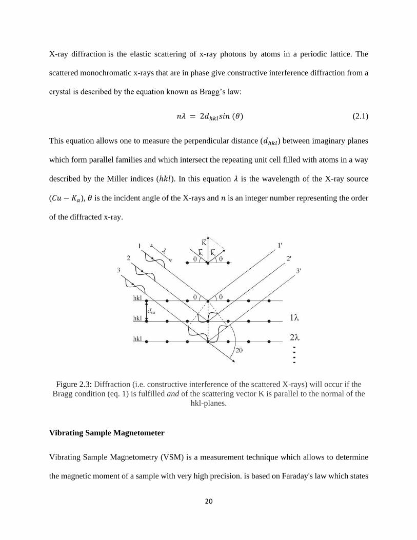
X-ray diffraction is the elastic scattering of x-ray photons by atoms in a periodic lattice. The

scattered monochromatic x-rays that are in phase give constructive interference diffraction from a

crystal is described by the equation known as Bragg’s law:

𝑛𝜆 = 2𝑑ℎ𝑘𝑙𝑠𝑖𝑛 (𝜃) (2.1)

This equation allows one to measure the perpendicular distance (𝑑ℎ𝑘𝑙) between imaginary planes

which form parallel families and which intersect the repeating unit cell filled with atoms in a way

described by the Miller indices (ℎ𝑘𝑙). In this equation 𝜆 is the wavelength of the X-ray source

(𝐶𝑢 − 𝐾𝛼), 𝜃 is the incident angle of the X-rays and 𝑛 is an integer number representing the order

of the diffracted x-ray.

Figure 2.3: Diffraction (i.e. constructive interference of the scattered X-rays) will occur if the

Bragg condition (eq. 1) is fulfilled and of the scattering vector K is parallel to the normal of the

hkl-planes.

Vibrating Sample Magnetometer

Vibrating Sample Magnetometry (VSM) is a measurement technique which allows to determine

the magnetic moment of a sample with very high precision. is based on Faraday's law which states

21

that an electromagnetic force is generated in a coil when there is a change in the magnetic flux

through the coil. In the measurement setup, a magnetic sample is moving in the proximity of two

pickup coils.

The oscillator provides a sinusoidal signal that is translated by the transducer assembly into a

vertical vibration. The sample which is fixed to the sample rod vibrates with a given frequency

and amplitude. It is centered between the two pole pieces of an electromagnet that generates a

magnetic field H0 of high homogeneity.

Stationary pickup coils are mounted on the poles of the electromagnet. Their symmetry center

coincides with the magnetic center of the static sample. Hence, the change in magnetic flux

originating from the vertical movement of the magnetized sample induces a voltage Vind in the

coils. 𝐻0, being constant, has no effect on the voltage but is necessary only for magnetizing the

sample. According to Faraday, the voltage in a single winding of the pickup coil can be written as

𝑉𝑖𝑛𝑑 = − 𝜕Φ 𝜕t⁄ (2.2)

where Φ is the magnetic flux. For nc pickup coils with a flat surface A and nw windings, the induced

voltage would be

𝑉𝑖𝑛𝑑 = ∑ ∑ ∫ (𝜕Φ 𝜕t⁄ )𝑑𝐴𝐴𝑛𝑤𝑛𝑐

(2.3)

Where B is the magnetic flux density

22

Figure 2.4: Schematic representation of a Vibrating sample Magnetometer (VSM).

Magnetic Measurements for Magnetocaloric Effect

Direct Measurement

In the direct measurements of the MCE, the magnetocaloric material is exposed to an external

magnetic field change and at the same time its temperature change Δ𝑇 is being registered using a

thermal sensor that is directly in contact with the MCM. The adiabatic temperature change is given

by

Δ𝑇(𝑇0, ΔH) = 𝑇𝐹(𝐻𝐹) − 𝑇𝐼(𝑇𝐼) ; Δ𝐻 = 𝐻𝐹−𝐻𝐼 (2.4)

A direct measurement of the change in temperature (Δ𝑇) has been built based on the design

proposed by Gopal et al., for the analysis of a Gd 99.9% sample. The accuracy of the Δ𝑇 measure

is dependent in a lot of variables in the set-up, like the setting of the magnetic field, thermometry

and the insulation of the sample, usually in the 5-10% error range.

23

Figure 2.5: Adiabatic temperature change during a magnetic field change of 1.1 T for a test

sample of Gd 99.9 %. Taken from [18].

Indirect Measurement

To obtain the magnetocaloric effect through indirect methods, it is necessary to do magnetization

and heat capacity measurements in order to be able to use the thermodynamic equations obtained

in Chapter 1. This method is the most seen in published investigations on the magnetocaloric

effect, and is based on magnetic measurements for the calculation of magnetic entropy changes.

Figure 2.6: Experimentally observed magnetization M in melt-spun LaFe11.6Si1.4 showing a weak

first order transition in dependence on (a) temperature and (b) magnetic field. Taken from [8].

24

DC magnetic measurements (magnetization vs temperature at constant magnetic field and

magnetization vs field at constant temperatures) are needed in order to calculate the magnetic

change in entropy. A magnetization vs. temperature measurement is first needed to determine the

temperature at which the MCM undergoes a phase transition, once this temperature has been

identified, magnetization vs. field measurements at different temperatures intervals around the

phase transition must be done, following equation. (1.20)

∆𝑆 = ∆𝑆𝑚 = − ∫ (𝜕𝜎 𝜕𝑇⁄ )𝐻1

𝐻0

𝑑𝐻 = 𝑀𝐶𝐸𝑖𝑠𝑜𝑡

Figure 2.7: Process for calculating the magnetic change in entropy with the indirect method. (a)

Magnetic isotherms are measured. (b-c) Entropy at each temperature is calculated. (d) Difference

of magnetic entropy is obtained.

25

The process for calculating the magnetic change in entropy with the indirect method is illustrated

in Figure 2.7, first different magnetic isotherms at increments of 5K in temperature are measured,

with the help of Maxwell’s magnetic relations, the entropy at each temperature is calculated by

integrating each isotherm and finally the difference between neighboring isotherms is obtained

and plotted, resulting in the change in magnetic entropy ∆𝑆𝑚 graph.

26

Chapter 3: Synthesis, Magnetic and Magnetocaloric Properties of MnFe2Ga

Alloy

Introduction

In this chapter, we study the magnetocaloric effect (MCE) in the MnFe2Ga Heusler alloy by means

of studying the magnetization 𝑀(𝐻, 𝑇) of the sample around its phase transition temperature. It’s

found that this compound possesses two transitions temperatures, one around room temperature

(320𝐾) and another one at 550𝐾. For the transition at 320𝐾 under a field of 3𝑇 it is found to have

an inverse change in entropy ∆𝑆𝑀 with a value of 1.97 𝐽 𝑘𝑔−1𝐾−1 and a negative change of

4.60 𝐽 𝑘𝑔−1𝐾−1 for the high temperature transition, with a Relative Cooling Power (RCPFWHM) of

275.85 𝐽 𝑘𝑔−1 and 351.42 𝐽 𝑘𝑔−1, respectively. These results show a considerable MCE until

now not reported for this alloy, and with a plus of having two peaks for the change in entropy our

alloy provides us with the possibility of applications in extreme conditions (whereas military or

aero-spatial) for the cooling of a system which is desired to bring it to room temperature.

Experimental Details

Ingots of MnFe2Ga were prepared by arc melting up to 4 times the composing elements in an argon

atmosphere, afterwards the ingots were made ribbons by melt spinning and later annealed at 400C

at increasing intervals of two hours. Structural properties were studied by X-ray diffraction at room

temperature using a Bruker X-ray diffractometer with a Cu-K alpha radiation source. Transition

temperatures were determined by differential scanning calorimetry (DSC), also, magnetic

characterization was performed to obtain magnetic transitions in the temperature range of 50K to

800 K with a vibrating sample magnetometer (Versalab Three, Quantum Design) for the annealed

27

ribbons at a constant field strength of 100Oe. Afterwards, magnetic isotherms were performed in

the temperature range of 50-800K at increasing intervals of 5K in a magnetic field strength from

minus 3T to 3T for the calculation of the change in magnetic entropy around the phase transition

temperatures.

Results and Discussion

Figure 3.1 displays the powder XRD patterns at room temperature of the MnFe2G ribbons. XRD

analysis shows that the sample crystallizes mainly into the L21 crystallite cubic structure

(AlCu2Mn-type) corresponding to a full Heusler alloy compound

Figure 3.1: X-ray diffraction pattern of samples at room temperature.

From the magnetic characterization dependence (MxT) in Figure 3.2, it’s observable that the alloys

undergo two independent phase transitions, one that is around room temperature (~325K) and the

28

other at high temperature (~550K). From the nature observed in the hysteresis loops (Figure 3.4)

measurements at different temperatures it was observed a Ferrimagnetic to Ferromagnetic

transition from low to room temperature and from Ferromagnetic to Paramagnetic transition at

high temperature, matching the noticed transitions on the magnetization against temperature plot.

DSC analysis in Figure. 3.3 displays a more accurate values for the transitions in all the samples,

T1 being the ferrimagnetic to ferromagnetic, TM the beginning of the martensitic transition and TC

the Curie temperature.

From Arrot plots (Figure 3.5) it’s determined that the transition at room temperature is a first order

transition and the high temperature transition is found to be a second order one.

Figure 3.2: Magnetization dependence on temperature at a constant field of 100Oe.

29

Figure 3.3: Differential scanning calorimetry measurements for the annealed ribbons, showing

the low, Martensitic and Curie transition temperatures.

Following the process for the indirect method described in the previous chapter, magnetic

isotherms at increments of 5K in temperature in an external field up to 3T are measured in a range

of temperature from 50K to 800K for each of the annealed ribbons (Figure 3.4), magnetic entropy

is calculated with the help of Maxwell’s magnetic relations and then the change in magnetic

entropy is calculated (3.6).

30

Figure 3.4: Hysteresis loop of the ribbon annealed for two hours, at different temperatures in

intervals of 5 K. (a) From 50 to 400 K and (b) from 300 to 800K.

Figure 3.5: Arrot plots around phase transition temperatures, showing a first order transition at

320K and a first order transition at 550K.

Values for the maximum change in magnetic entropy around room temperature ferri-ferro

transition are found to be positive, 1.79 𝐽 𝑘𝑔−1𝐾−1 at 282.5 K, 1.97 𝐽 𝑘𝑔−1𝐾−1 at 287.5K,

1.44 𝐽 𝑘𝑔−1𝐾−1 at 277.5K, 1.81 𝐽 𝑘𝑔−1𝐾−1 at 282.5 K, 1.44 𝐽 𝑘𝑔−1𝐾−1 at 277.5K and

0.90 𝐽 𝑘𝑔−1𝐾−1 at 267.5K for the ribbon as is, the sample at annealing time of 2hrs, 4hrs, 6hrs

31

and 8hrs, respectively. The values for the change in entropy for the high temperature martensitic

transition are negative, all occurring at the same temperature of 577.5K, the corresponding −∆𝑆𝑀

values are 4.37 𝐽 𝑘𝑔−1𝐾−1, 4.60 𝐽 𝑘𝑔−1𝐾−1, 4.33 𝐽 𝑘𝑔−1𝐾−1, 4.59 𝐽 𝑘𝑔−1𝐾−1 and

4.58 𝐽 𝑘𝑔−1𝐾−1.

Fig 3.6. Change in entropy for all the ribbon samples at a 0-3T external field strength.

Table 3.1: Transition temperature T1, change in entropy and relative cooling power at the near room temperature.

Compound 𝑇1 ∆𝑆 (3T) RCP

Ribbon as is 325 1.79 79.93

Annealed 2 hrs 325 1.97 275.85

Annealed 4 hrs 325 1.81 342.30

Annealed 6 hrs 325 1.44 354.95

Annealed 9 hrs 325 0.90 252.60

32

Table 3.2: Curie transition temperature Tc, change in entropy and relative cooling power at the

high temperature.

Compound 𝑇𝐶 ∆𝑆 (3T) RCP

Ribbon as is 552 4.37 330.69

Annealed 2 hrs 552 4.60 351.42

Annealed 4 hrs 552 4.33 242.20

Annealed 6 hrs 552 4.59 379.25

Annealed 9 hrs 552 4.58 314.56

For their cooling effectiveness the Relative Cooling Power (RCP) is calculated using the formula

𝑅𝐶𝑃 = ∆𝑆𝑀 × ∆𝑇𝐹𝑊𝐻𝑀

Where ∆𝑇𝐹𝑊𝐻𝑀 is the temperature full range at half the maximum change in entropy on the ∆𝑆𝑀

peaks. Values of 79.93 𝐽 𝑘𝑔−1, 275.85 𝐽 𝑘𝑔−1, 342.30 𝐽 𝑘𝑔−1, 354.95 𝐽 𝑘𝑔−1 and

252.60 𝐽 𝑘𝑔−1 of RCP for the original ribbon, and samples annealed at 2, 4, 6 and 8 hrs

respectively at room temperature transition. For the martensitic transition RCP values of

330.69 𝐽 𝑘𝑔−1, 351.42 𝐽 𝑘𝑔−1, 242.20 𝐽 𝑘𝑔−1, 379.25 𝐽 𝑘𝑔−1 and 314.56 𝐽 𝑘𝑔−1 were

obtained.

These RCP values show that even though the value for the change in entropy on our samples is

relatively small for the room temperature and medium values for the high temperature, the samples

are a good contender to be applied as a magnetocaloric material.

Conclusion

The focus in this thesis has been to develop a new alloy for magnetocaloric effect applications.

The work began by synthetizing the Fe2MnGa alloy and determining its feasibility to be applied

as a magnetocaloric material by studying its structural and magnetic properties.

33

Fe2MnGa ingots that prepared via arc melting, later melt spinned and afterwards annealed at 400C

at increasing times, magnetic and calorimetric analysis did show two magnetic transitions in this

alloy system, going from low to high temperature a magnetic phase transition is observed, going

from a ferrimagnetic to ferromagnetic state and another transition is observed at high temperature,

going from a ferromagnetic to paramagnetic phase due to a martensitic transition proper of memory

shape alloys. The values obtained for the magnetic change in entropy, shows medium changes in

entropy in both transitions and good RCP values were obtained for the room temperature transition

as the operational range ∆𝑇𝐹𝑊𝐻𝑀 of temperature increased with the annealing time, as for the high

transition temperature the magnetic change in entropy remained somewhat constant with medium-

high values for the entropy, and therefore also constant RCP values. With this alloy system

characterization finished, we can conclude that the Fe2MnGa alloy may have applications as a

magnetocaloric material for magnetic refrigeration in everyday applications at room temperature

and extreme conditions (high temperature).

34

References

1. Tishin, A.M. & Spichkin, Y.S. (2003) The magnetocaloric effect and its applications.

Philadelphia, PA: IOP Publishing.

2. GE Appliances (2014, March 14). From Ice Blocks to Compressors to Magnets: The Next

Chapter in Home Refrigeration from GE, Retrieved from

https://www.businesswire.com/news/home/20140313005901/en

3. Department of Energy (2017, December). Energy Savings Potential and RD&D

Opportunities for Commercial Building HVAC Systems (pp. 80), Retrieved from

https://www.energy.gov/sites/prod/files/2017/12/f46/bto-DOE-Comm-HVAC-Report-12-

21-17.pdf

4. Behzad Monfared (2018), Design and optimization of regenerators of a rotary magnetic

refrigeration device using a detailed simulation model, International Journal of

Refrigeration, DOI: 10.1016/j.ijrefrig.2018.01.011

5. Zhang, Mingkan; Mehdizadeh Momen, Ayyoub; & Abdelaziz, Omar (2016), "Preliminary

Analysis of a Fully Solid State Magnetocaloric Refrigeration". International Refrigeration

and Air Conditioning Conference. Paper 1758. Retrieved from

http://docs.lib.purdue.edu/iracc/1758

6. J Inoue & M Shimizu (1982), Volume dependence of the first-order transition temperature

for RCo2 compounds, Journal of Physics F: Metal Physics, Volume 12, Number 8, DOI:

10.1088/0305-4608/12/8/021

7. Banerjee, B. K (1964), On a generalised approach to first and second order magnetic

transitions. Physics Letters, Volume 12, Issue 1, p. 16-17 DOI: 10.1016/0031-

9163(64)91158-8

35

8. Julia Lyubina (2017), Magnetocaloric materials for energy efficient cooling, Journal of

Physics D: Applied Physics, Volume 50, Number 5, DOI: 10.1088/1361-

6463/50/5/053002

9. W. F. Giauque & D. P. Macdougall (1933), Attainment of Temperatures Below 1°

Absolute by Demagnetization ofGd2(SO4)3·8H2O, Physical Review. Volume 43,

Number, DOI: 10.1103/PhysRev.43.768.

10. V. Franco et al. (2018), Magnetocaloric effect: From materials research to refrigeration

devices Progress in Materials Science, Volume 93, DOI: 10.1016/j.pmatsci.2017.10.005

11. Li Ling-Wei, Review of magnetic properties and magnetocaloric effect in the

intermetallic compounds of rare earth with low boiling point metals, Chinese Physics B,

Volume 25, DOI: 10.1088/1674-1056/25/3/037502

12. J. Romero Gomez et al. (2006), Magnetocaloric effect: A review of the thermodynamic

cycles in magnetic refrigeration, Renewable and Sustainable Energy Reviews, Volume

17, DOI: 10.1016/j.rser.2012.09.027

13. I Galanakis et al. (2006), Electronic structure and Slater–Pauling behaviour in half-

metallic Heusler alloys calculated from first principles, Journal of Physics D: Applied

Physics, Volume 39, DOI: 10.1088/0022-3727/39/5/S01

14. Heusler, F. (1903). Über magnetische manganlegierungen. Verhandlungen der Deutschen

Physikalischen Gesellschaft, Volume 5.

15. Potter, H. H. (1928). The X-ray structure and magnetic properties of single crystals of

Heusler alloy. Proceedings of the Physical Society, Volume 41, DOI: 10.1088/0959-

5309/41/1/314.

36

16. Qian, Hui et al. (2013). Recentering Shape Memory Alloy Passive Damper for Structural

Vibration Control. Mathematical Problems in Engineering, DOI: 10.1155/2013/963530

17. Rong Chuanbing & Shen Baogen (2018). Nanocrystalline and nanocomposite permanent

magnets by melt spinning technique. Chinese Physics B, Volume 27, DOI: 10.1088/1674-

1056/27/11/117502

18. Gopal, B. R., Chahine, R., & Bose, T. K. (1997). A sample translatory type insert for

automated magnetocaloric effect measurements. Review of scientific instruments,

Volume 68, DOI: 10.1063/1.1147999

37

Vita

Eduardo Martinez Teran earned a Bachelor of Science degree in Physics from Universidad de

Sonora, Hermosillo, Sonora. He joined UTEP’s master program in Physics in spring 2018.

While pursuing his degree, Eduardo has authored and co-authored 3 peer reviewed publications

in international journals. He also presented his research findings at international conferences

including MMM and IEEE-MMM Joint Conference for which he received a Student Travel

Award.

Contact Information: emartinezt@miners.utep.edu