DEPARTMENT OF TECHNOLOGY AND BUILT ENVIRONMENT

Near-Field Characterization of FM Transmitter Devices in

Mobile Phone Applications

Mst. Afroza Khatun

September, 2008

Master’s Thesis in Electronics/Telecommunication

Examiner: Professor Claes Beckman, University of Gavle, Sweden

Supervisor: Nikolay Serafimov, Sony Ericsson Mobile Communications ,Lund, Sweden Co-supervisor: Zhinong Ying, Sony Ericsson Mobile Communications ,Lund, Sweden

Master Thesis Near-Field Characterization of FM Transmitter Devices in Mobile Phone Applications

By

Mst. Afroza Khatun

Sony Ericsson Mobile Communications AB SE-221 88 Lund, Sweden

in cooperation with

Department of ITB/Electronics

University of Gävle SE- 801 76 Gävle, Sweden

Gävle, September 2008

The God has blessed me

With a wonderful family

To whom this thesis paper is dedicated

v

Abstract Mobile Phone, without this we can’t think to pass a day in presence. We have found a rapid increase of

mobile phone users from a few years ago till now. Day by day the modern technologies allow the mobile

phone to become smaller, cheaper, and more reliable. This also creates new possibilities for applications

and integrations of the classical broadcast systems and modern mobile phone technologies. One example

is the FM transmitter in mobile phone. The FM transmitter in a mobile phone is a “cool” feature which

allows listening to the music content in phone on a car or home radio.

This thesis work deals with the near field characterization of FM transmitters in mobile phone

applications. The RF scientists and engineers neglect the near field zone because typical RF links operate

at distances of many wavelengths away where near field effects are totally insignificant. But in this work

we are interested in the near field properties of the FM transmitter. We measured the field intensity at

near field and estimated the field strength at the far field region at 3 meters. To measure the field intensity

and the effective radiated power we used HR1 near field scanner. As this is a new measurement approach,

we made the validation of this system by measuring a reference dipole antenna at 880MHz and then

compare the measured results to the CST simulation results. A basic phone model of FM transmitter has

been created by CST simulation and a prototype has been made which was also used as our DUT. After

validation of the near field measurement system we measured our DUTs (3 models-one cable fed

prototype and two active devices) with the near field system and estimate the effective radiated power and

field intensity at 3 meter. Furthermore, we measured our DUTs at 3 meter with a far field measurement

system with optical fiber connection. A feasible relation between field strength and measured power was

defined in order to correlate the near field scanner results with the far field measurement system.

This paper also provides a short design guide line for built in FM antennas by relating the antenna size

and placement to input power and the field strength in mobile phone FM transmitter application.

vii

Preface This report is the result of a Master’s thesis, performed at Sony Ericsson Mobile Communication, Lund, Sweden and presented at the department of ITB/Electronics of the University of Gävle, Sweden. I was at University of Gävle as a foreign Student in ITB/Electronics department and I come from Bangladesh. The examiner was Professor Claes Beckman at the department of ITB/Electronics and the work was supervised by Nikolay Serafimov, Staff Engineer on Terminal Antennas development unit at Sony Ericsson Mobile Communications AB, Lund, Sweden. This work was done from March 2008 to July 2008. The thesis project was financed by Sony Ericsson Mobile Communication, Lund, Sweden. The EMC HR1 scanner used during the work was designed, manufactured by Detectus AB (www.detectus.com).

ix

Acknowledgment First, I would like to thank my supervisor Nikolay Serafimov. He energetically involved himself in the

project and offered his valuable time, extensive co-operation, guidance, encouragement, useful support at

every stage of my project. I appreciate this wonderful opportunity to study and work under his

supervisions.

I wish to express my warm and sincere thanks to my co-supervisor, Zhinong Ying, Antenna Expert,

Antenna Technology section, SEMC, Lund, Sweden. His valuable advice and friendly help is really

remarkable. His extensive discussion around my work has been also a great value of my project.

I need to be grateful to Thomas Bolin, Technical Manager of the Terminal Antennas Development Unit,

SEMC, Lund, Sweden for giving the chance to make my Master’s thesis in his research group and also

for helping and encouraging during the time of preparing this thesis work.

I am grateful to Andre da Silva Frazao for introducing me to my Manager, Thomas Bolin. I would also

like to acknowledge to all the members at SEMC for their help and availability, especially Katsunori

Ishimiya, Jonas Långbacka, Jesper Petersson.

Professor Claes Beckman who is my examiner of the thesis work. I would like to say he is not only my

examiner; he is the person who let me in to the world of antennas through the antenna course. I am really

grateful to him for his every support and guidance during my studies as well as my thesis work and still

now.

Special thanks go to all the responsible in the ITB/Electronics Departments of the University of Gävle. I

would like also to thank all the staff of the ITB/Electronics, respective teachers and all of my friends with

whom I spent my University years.

I owe my loving thanks to my parents, my brother and my sister for all their constant love, encouragement

and support which help me to pursue my academic goals. What I am now is due to them. Thanks to all the

family, I feel always like if you were beside me all the time despite of the distance.

I have been very fortunate that Dristy, my loving husband, has been such a strong support, patience, love,

inspiration, encouragement through all of the period. Without his encouragement and understanding it

would have been impossible for me to finish this work.

Table of Contents

1. Introduction ……………………………………………………………….………………… 1 1.1 Basic requirements for FM transmitter …………………………………………………. 2 1.2 Radiated power limits of the FM transmitter ...…………………………………………. 2 1.3 The Goal of the thesis work …………………………………………………………….. 3

1.5 Thesis outline…………………………………………………………………………..... 4

2. Theory ……………………………..…………………………………………...……………. 5 2.1 An Overview of Near Field Antenna Measurement…………………………………….. 5 2.2 Near field vs. Far- field …………………………………………………………………. 7 2.3 Field Region Definitions considering the antenna size ………........................................ 8

2.3.1 Antenna size, D>λ ...……………………………………………………………. 9

2.3.2 Antenna size, D<λ ……………………………………………………………… 10

2.3.2 Antenna size, D<<λ …………………………………………………………….. 10 2.4 Effective Isotropic Radiated Power (EIRP) and Effective Radiated Power (ERP) …….. 11 2.5 E field and H field Strength……………………………………………………………... 12 2.6 E field strength…………………………………………………………………………... 13 2.7 H field strength………………………………………………………………………….. 14 2.8 E field or H field………………………………………………………………………… 14

3. Measurement set up ...…………….………………………………......................................... 17

3.1 Near field measurement procedure design ...…………………………………………… 17 3.1.1 Setup for near field measurements with HR1 scanner ………………………….. 17 3.1.2 Near Field Probes Overview…………………………………………………….. 20 3.1.2.1 Property of the magnetic probe…………………………………………. 20 3.1.2.2 Properties of Electric field probe……………………………………….. 21 3.1.2.3 Basic Theory of Magnetic loop probes…………………………………. 22 3.2 Outdoors FF measurement systems for FM frequencies with Optical fiber connection... 23

4. Simulated results …… ...…………….……………………………….................................... 27 4.1 Simulation of half wave length dipole ………………….…………………………......... 27 4.1.1 Simulated field intensities ………………………………………………………. 29 4.2 Simulation of Basic FM Transmitter Phone Model……………………………………... 30 4.2.1 Phone model at resonance frequency …………………………………………….. 30 4.2.1.1 Simulated Field intensities ………………………………………................ 32

4.2.2 Phone model at FM frequency…………………………………………………….. 33

4.2.2.1 Simulated Field intensities…………………………………………………. 33 4.3 Hx or Hy or Hz Component……………………………………………………………... 34 4.4 Simulated Field strength and ERP up to 3 m for reference antennas…………………… 34

5. Measured Results ……………….……….………………………………... ……………….. 37 5.1 Reference Dipole antenna at 880 MHz ………………………..………………………... 37 5.2.1 Measured results.………………………………………………………………….. 37 5.1.2 Estimation of field intensities and radiated power at 3 m distance……………….. 39 5.1.3 Comparison between measured and simulated results …...……………… ……… 44 5.2 Phone model at 920 MHz……………………………………………………………….. 45 5.2.1 Measured results…………………………………………………………………... 45 5.2.2 Estimation of field intensities and radiated power at 3 m distance………………. 46 5.2.3 Comparison between measured and simulated results……………………………. 50 5.3 DUTs at 100MHz………………………………………………………………………. 50 5.3.1 The basic Phone Model at 100 MHz……………………………………………… 51 5.3.1.1 Measured result……………………………………………………………. 51 5.3.1.2 Estimation of field intensity and radiated power at 3 meter ……………… 52 5.3.2 Active DUT- 1(FM transmitter device)…………………………………………… 54 5.3.2.1 Measured result……………………………………………………………. 54 5.3.2.2 Estimation of field intensity and radiated power at 3 meter………………. 56 5.3.3 Active DUT-2 (FM transmitter)…………………………………………………... 57 5.3.3.1 Measured Results………………………………………………………….. 57 5.3.3.2 Estimation of field intensity and radiated power at 3 meter………………. 58 5.3.4 Comparison of the far field result to the near field scanner result of 3 different DUTs at 100 MHz………………………………………………………………... 59 5.3.5 ‘1 Meter measurement’ and comparison with previous results…………………… 61

6. Discussion……………………………………………………………………………………. 69 6.1 Measurement System feasibility………………………………………………………... 69 6.1.1 HR1 near field scanner…………………………………………………………….. 69 6.1.2 Outdoor Far field measurement system……………………………………………. 70 6.1.3 1 meter measurement system………………………………………………………. 70 6.2 Measurement of reference antennas using HR1 near field scanner…………………….. 71 6.2.1 Measurement of DUTs using HR1 near field scanner……………………………... 717. Conclusion and Future Research .......……………….……….……………………………. 73 7.1 Conclusion ……….………………………..………………….………………………... 73 7.2 Future research ……………………...………………………………………………….. 75References ...………………………………………………………………………………….… 77

Appendix A. Derivation of effective radiated power from E field intensity ………………..…. 79

Appendix B. Conversion……………………………………………………………………..… 81

Appendix C. Parameters table for outdoor Far field measurement system with optical Fiber connection………………………………………………………………………

83

Appendix D. Technical Data for the Tunable Dipole Antenna……………………………..… 85

Appendix E. Relation between field strength and volume of FM transmitter antenna………. 87

E.1 Antenna structures……………………………………………………………………….. 87 E.2 Results by simulations…………………………………………………………………… 88

Chapter 1

Introduction The ability to communicate with people on the move has developed outstandingly since Guglielmo

Marconi first demonstrated radio’s ability to provide continuous contact with ships sailing the English

Channel. That was in 1897, and since then new wireless communications methods and services has

been devotedly adopt by people throughout the world. As a result wireless communication over great

distance to a large number of people is not new. Wireless communications may be one-way

communications as in broadcasting systems (such as radio and TV), or two-way communication (e.g.

mobile phones).

The advances of the technologies like improvement of RF circuit fabrication, new large-scale circuit

integration and other miniaturization technologies allow the portable radio equipments to become

smaller, cheaper, and more reliable. This also creates new possibilities for application and integrations

of the classical broadcast systems and modern mobile phone technologies. FM transmitter is such a

device which gives the freedom of sending a wireless broadcast of any audio like music audio,

streaming audio, MP3 audio etc. to any FM radio anywhere in home, car or office.

The FM transmitter uses FM radio waves to send sound from one source to any nearby radio or stereo

system. Most often it is a short range low power FM transmitters operating in the FM Broadcast band

87.5 to 108 MHz. But in Japan the FM broadcast band is 76-90 MHz, unlike any other country in the

world.

In this study FM transmitter in mobile phone application will be considered. The FM transmitter in a

mobile phone allows listening to the music content in a phone on a car or home radio. For example,

the FM transmitter unit can be separate device that is attached to the mobile phone and then transmit

music over the air within the FM radio frequency band. Even more attractive is to have the FM

transmitter built inside the mobile phone. However this creates the need of strict FM transmitter

regulation to provide compatibility with the official broadcast systems. In addition to this not all

countries allow the legal use of FM transmitter devices. A brief discussion of the ETSI and FCC FM

transmitter regulations are given in the next session.

1

1.1 Basic requirements for FM transmitter:

According to European Telecommunications Standards Institute (ETSI) the following conditions shall

be met by the FM transmitter [1]:

FM Transmitter shall come to an end to transmit within 1 minute of the elimination of

audio modulation.

The transmitter should have an integral antenna, is permanent fixed antenna built in,

designed as an indispensable part of the equipment.

The user interface of the FM transmitter shall permit as a minimum frequency ranges

within 88.1 MHz to 107.9 MHz and as a maximum 87.6 MHz to 107.9 MHz frequency

The FM transmitter shall operate on selectable frequencies within the specified frequency

range using a 50 kHz, 100 kHz or 200 kHz frequency step size.

1.2 Radiated power limits of the FM transmitter:

As a FM transmitter is short range low power equipment so there is a limitation for the effective

radiated power and field strength. The limits are as follows according to ETSI [1] and FCC [2].

Standard Effective radiated Power(ERP) limit

Radiated field strength at 3 meter

Radiated field strength at 10 meter

ETSI -43 dBm(50 nW) 52.2 dBuV/m 42.2 dBuV/m

FCC -52.43dBm(5.7 nW) 47.9 dBuV/m -

Table 1.1* Limits of transmitter parameters of FM transmitter according to ETSI

The maximum acceptable measurement uncertainty for effective radiated power should be 6 dB. ±

The limits are specified at 3 meters which is in far field region for a small antenna at FM frequency.

In mobile phone application a FM antenna would normally have dimensions less than 10/λ and

therefore the distance at 3 meters is better than which is the boundary for far field region and

as a consequence can be considered as being in the far field. The details of the field region of small

antenna are discussed in chapter 2.

λ/2 2d

2

* Note: Some inconsistency was found in the ETSI in case of ERP, EIRP (Equivalent Isotropic Radiated Power)

derivation. Detailed motivation is given in chapter 2.

1.3 The Goal of the thesis work: The FM transmitter in a mobile phone is a “cool” feature. However, the FM frequency propagation

puts constraints on how to characterize a FM transmitter device. In this thesis work a new

measurement approach is studied. Instead of classical far field measurements we can sense the near

field of a FM transmitter device and then convert this result to field strength at the desired distance. In

this case we would avoid the physical FM measurements limitations like minimum chamber size,

absorbers etc. Our intention is to use HR1 near field scanner (High Resolution EMC Scanner) to

measure the field strength and then convert to ERP of the FM transmitter. Initially near field Scanner

measurements will be compared with corresponding CST (Computer Simulation Technology)

simulations. Then a feasible relation between the absolute field strength and measured power will be

defined in order to correlate the near field scan results with an outdoor far field measurement system

with the optical fiber connection. For this purpose we will use several DUTs (Device Under Test) –

active and passive. Besides these another outcome will be defined such as the relation between ERP

or field strength and volume of the FM transmitter antenna. The schematic block diagram of our thesis

work is shown below.

Figure 1.1 Schematic block diagram of the thesis work

3

1.4 Thesis outline:

Firstly Chapter 1- Introduction - presents the basic concept of FM transmitter, background of near

field measurement, goal and problem statements.

Chapter 2- Theory- contains the advantages and disadvantages of near field and far field

measurements, the field region definitions depending on antenna size, antenna field strength and

radiated power calculations.

Chapter 3- Measurement set up-explains the technical and theoretical information regarding HR1

near field scanner. In addition the outdoor far field measurement with optical fiber connection is

explained.

Chapter 4- Software simulation- CST simulation of balanced half wavelength dipole antenna, basic

phone model of FM transmitter and describes the simulated results.

Chapter 5- Measurement results- contains all measured result for reference antenna as well as the

different DUTs, comparison between the simulation and measurements for reference antenna and

between near field measurement and far field measurement for DUTs.

Chapter 6- Discussion- describes the measurement systems feasibility.

Chapter 7- Conclusion- presents the conclusions from the analysis of measured result as well as the

whole thesis work. Future work is also suggested.

4

Chapter 2 Theory

Before going to details on the theory which is used in this study one thing is needed to clarify related

to ETSI standard describes in previous chapter. It is said that there is some inconsistency is discovered

in the ETSI standard for ERP and EIRP calculation. According to the antenna theory ERP is 2.15 dB

smaller than the EIRP (details are in section 2.4). But in ETSI standard ERP is 2.15 dB higher than

EIRP. So if the ERP limit is taken -43 dBm then the field strength corresponding will change. The

corrected limits of FM transmitter are given in table 2.1. The calculation procedure is in Appendix A.

Effective radiated Power(ERP) limit

Radiated field strength at 3 meter

Radiated field strength at 10 meter

-43 dBm(50 nW) 57.39 dBuV/m 47.39 dBuV/m

Table 2.1 Corrected limits of transmitter parameters of FM transmitter

Now it could be interesting to have a look the overview of near field measurement.

2.1 An Overview of Near Field Antenna Measurements:

According to the time divisions the development of near field scanning as a method for measuring

antennas can be divided suitably into four periods: the early experimental period with no probe

correction (1950-1961), the period of the first probe-corrected theories (1961-1975), the period in

which the first theories were put into practice (1965-1975), and the period of technology transfer

(1975-1985) in which 50 or more near field scanners were build throughout the world [3].

i. Early experiment period(1950-1961):

“Automatic antenna wave front plotter” is probably the first near field antenna scanner which is

built around 1950 by Barrett and Barnes of the Air Force Cambridge Research Center. In spite of

they did not make any attempt to compute the far field patterns from their measured near field

data, Barrett and Barnes obtained full size maps of the phase and amplitude variations in front of

5

microwave antennas. In 1953 Woonton examined the assumption that the voltage induced in the

probe is a measure of the electric field strength. In 1961 Clyton Hollis and Teegardin computed

the principal far field E plane pattern for a 14 wave length diameter reflector antenna from the

amplitude and phase of the near field distribution.

ii. First Probe Corrected theories (1961-1975):

In the early period, all the experimental work assumed basically that the probe measured a

rectangular component of the electric or magnetic vector in the near field. In 1961 Brown and

Jull gave a rigorous solution to the probe correction problem in two dimensions using cylindrical

wave functions to expand the field of the test antenna but plane waves to characterize the probe.

“Plane-wave scattering –matrix theory of antennas and antenna-antenna interactions” is the

definitive work on the theory of planner near field scanning which is provided by Kerns’s

National Bureau of Standards (NBS). Recently, Yaghjian and Wittmann have derived a

simplified probe corrected spherical transmission formula in terms of conventional vector

spherical waves. Yaghjian also suggests a direct computation scheme for evaluating the θ

integrations.

iii) Theory Put into Practice(1965-1975):

The first probe corrected near field measurements were handed at the National Bureau of

Standards in 1965 using lathe bed to scan on a plane in front of a 96 wave length pyramidal horn

radiating at a frequency of 47.7 GHz [3]. From 1965 more than 10 years following the probe

corrected near field scanning was confined for planner and cylindrical scanning. In this period

some development were built like

a. Sampling theorems were applied to determine data point spacing,

b. Efficient methods of computation were employed,

c. Automatic computer controlled transport of the test antenna and probe was installed ,

d. Lasers were used to accurately measure the position of the probe and

e. Upper bound theoretical as well as experimental and computer-simulated error analyses

were performed.

6

iv) Technology Transfer (1975-1985): The recent interest in the near field measurements has been generated primarily by the

development of modern, specially designed antennas that are not easily measured on

conventional far field ranges [3]. Near field measurement was used in a sophisticated procedure

for aligning the beam formers of large, scanning phased array antennas. Computation of the array

excitation coefficients by taking the Fourier transform of the complex array factor, the far field

data is computed from planner near field measurements. The entire fundamental period of the

array factor is obtained by steering the array to two or more positions and then recording the near

field data for each position. The element pattern can also be evaluated by steering the array during

its planner near field measurement and computing the peak values of the steered far field patterns.

2.2 Near field vs. Far- field:

With appropriate measurement system, any antenna can be successfully measured on either near field

or far field range. Actually there are some significant factors like cost, size etc which leads to

recommend of one over the other. Usually, for high frequency antennas where complete pattern and

polarization measurements are required near field ranges are better choice while for low frequency

antennas where simple pattern cut measurements are required far field ranges are better choice [4].

As it is mentioned before each measurement has certain advantages and disadvantages and this makes

generalized comparisons between near field and far field techniques. Far field measurements have

several disadvantages over near field which makes the near field measurement more expectant. The

advantages of near field include:

The complete characterization of the DUT is performed.

Test site location is convenient- the near field system needs less space compare to far field

measurement.

Negligible real estate requirement- does not need large chamber, absorbers etc.

Nominal multipath problems- like far field the multipath propagation is not effect the

measurements.

Removal of weather effects- like outdoor far field measurements no need to give attention to

the weather condition.

7

Stationary antenna (planner near–field configuration)- for planner near field measurement

system the orientation of the DUT as well as the probe antenna is not complex.

Quick measurement- the measurement time is comparably less.

Need simple modification to shape the complete measurements.

Basically, near field measurement provide the necessary information to determine the radiating field

at the surface of the antenna. See figure 2.1 this process is called microwave holography and involves

the transformation of the near field data to any arbitrary location. The most commonly used near-field

techniques are planner, cylindrical and spherical. This paper discusses primarily the planar

configurations.

2.3 Field Region Definitions considering the antenna size:

The space surrounding an antenna is usually can be divided into two main regions as shown in figure

2.1 far field (Fraunhofer) and near field. Near field region includes two sub regions: (a) reactive near

field, (b) radiating near field (Fresnel).

Figure 2.1 Exterior fields of radiating antenna [3]

These regions are designed in such a way that provides the identification of field structure in each

region. The boundary of the field region is not fixed for all antennas rather than they have great

8

dependency on the antenna size. Let’s see the boundary of these three regions considering the antenna

size.

2.3.1 Antenna size, D>λ :

The transitions between the three regions are not distinct but gradual. In the reactive near field region

energy is stored in the electric and magnetic fields very close to the source. They are not the radiating

fields. The strict IEEE definition is "That portion of the near-field region immediately surrounding

the antenna, wherein the reactive field dominates.”[5]. The approximate outer edge of the reactive

near field for electrically large antennas is given by

λ31 62.0 DR < 2.1

where D is the largest dimension of the antenna and λ is the wavelength. In the reactive region, the

field intensity decays very rapidly with distance from the antenna.

In the radiating near field, the angular field distribution depends on distance from the RF source

unlike in the far field where it does not [6]. The strict IEEE definition is "That portion of the near

field region of an antenna between the far field and the reactive portion of the near field region,

wherein the angular field distribution is dependent upon distance from the antenna." [5]. Energy is

radiated as well as exchanged between the source and a reactive near field. The outer boundary of this

region for an electrically large antenna is:

λ

2

22DR ≈ 2.2

In the far field, electric and magnetic fields propagate outward as an electromagnetic wave and are

perpendicular to each other and to the direction of propagation. In this region the angular field

distribution is independent of the distance from the antenna. The strict IEEE definition is "That region

of the field of an antenna where the angular field distribution is essentially independent of the

distance from a specific point in the antenna region."[5]. The far field region is sometimes termed the

Fraunhofer region in analogy with Fraunhofer diffraction. In the far field region the field components

are orthogonal. The distribution of fields and power density is independent of distance. The electric

and magnetic fields decay inversely with distance from the antenna and power density decays as the

inverse square of the distance.

9

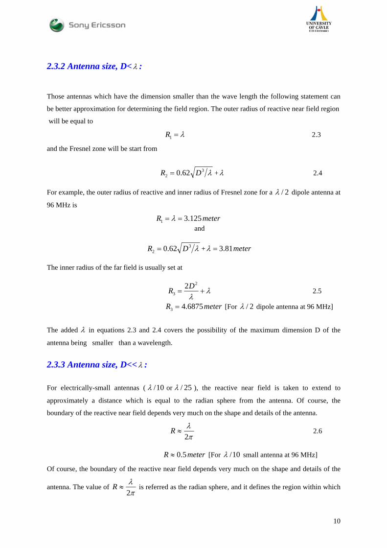
2.3.2 Antenna size, D<λ :

Those antennas which have the dimension smaller than the wave length the following statement can

be better approximation for determining the field region. The outer radius of reactive near field region

will be equal to

λ=1R 2.3

and the Fresnel zone will be start from

λ32 62.0 DR = +λ 2.4

For example, the outer radius of reactive and inner radius of Fresnel zone for a 2/λ dipole antenna at

96 MHz is

meterR 125.31 == λ and

λ32 62.0 DR = + meter81.3=λ

The inner radius of the far field is usually set at

λλ

+=2

32DR 2.5

meterR 6875.43 = [For 2/λ dipole antenna at 96 MHz]

The added λ in equations 2.3 and 2.4 covers the possibility of the maximum dimension D of the

antenna being smaller than a wavelength.

2.3.3 Antenna size, D<<λ :

For electrically-small antennas ( 10/λ or 25/λ ), the reactive near field is taken to extend to

approximately a distance which is equal to the radian sphere from the antenna. Of course, the

boundary of the reactive near field depends very much on the shape and details of the antenna.

πλ

2≈R 2.6

meterR 5.0≈ [For 10/λ small antenna at 96 MHz]

Of course, the boundary of the reactive near field depends very much on the shape and details of the

antenna. The value of πλ

2≈R is referred as the radian sphere, and it defines the region within which

10

the reactive power density is greater than the radiating power density. For an antenna the radian

sphere represents the volume occupied mainly by the stored energy of the antenna’s electric and

magnetic fields. Outside the radian sphere the radiated power density is greater than the reactive

power density and begins to dominate as πλ

2>>R [7].

Electrically-small antennas, for the most cases, do not exhibit radiating near field regions; rather, the

reactive near field transitions directly to the far field. Using the equation 2.1 and 2.2 it is noticed that

for a sufficiently small antenna it is shown that

λπ

λ 222

D> And λ

πλ 362.0

2D>

For electrically small antennas, the radiating near field is negligible if it exits at all. So, the behavior

of these antennas can be effectively described by two regions where electrically large antennas may

require three. For more details on the matter are given in reference [7].

2.4 Equivalent Isotropic Radiated Power (EIRP) and Effective Radiated Power (ERP):

An isotropic radiator is an ideal antenna which radiates power with unity gain which is uniformly

distributed in all directions and is generally used to reference antenna gains in wireless systems. The

equivalent isotropic radiated power (EIRP) for a given test antenna can be defined as:

tt GPEIRP += [In dB scale] 2.7

It represents the maximum radiated power available from the transmitter in the direction of maximum

antenna gain as compared to an isotropic radiator.

The land mobile industry has almost universally expressed effective radiated power (ERP) instead of

EIRP to denote the maximum radiated power as compared to a half-wave dipole antenna. Since a

dipole antenna has a gain of 1.64 (2.15 dB above an isotropic), the ERP will be 2.15 dB less than the

EIRP for the same transmission system [8].

15.2−= EIRPERP [In dB scale] 2.8

11

Figure 2.2 Gain in dBd vs. dBi

2.5 E field and H field Strength: Before entering into the heart of the theoretical aspect of this thesis, it might be useful to dedicate a

small session to some general considerations on the Electromagnetic field theory and other related

techniques. Thus, although many points have already been widely developed in various excellent

references, they are presented here directly in perspective of this thesis.

The unavoidable first step of this work is to write the fundamental Maxwell’s equations, as they are at

the basis of all the Electromagnetic theory. All the considerations, developments and discussions

presented in Electromagnetic theory are only the refinements of the fundamental four equations

governing the behavior of the Electromagnetic field.

Fundamental equations: Maxwell’s equations: Maxwell’s four equations are the fundamental relations that govern the behavior of the Electric and

Magnetic fields in the presence of sources. The differential forms of Maxwell’s equations are as

follows [10]:

2.9(a) 2.9(b)

2.9(c) 2.9(d)

[ ]

[ ][ ]

[ ]echmagneticisolatedNoB

lawsGaussD

lawcircuitalsAmperetDJH

lawsFaradaytBE

arg0

'

'

'

=⋅∇

=⋅∇∂∂

+=×∇

∂∂

−=×∇

ρ

t

J∂∂

−=⋅∇ρ

[Continuity equation] 2.10

12

Where the terms are: t, time dependency E, the electric field intensity [volt/meter]

H, the magnetic field intensity [ampere/meter]

J, the density of free current [ampere/meter ] 3

D, the electric flux density [colomb/meter ] 2

B, the magnetic flux density [weber/meter 2 ]

ρ , the volume density of free charge

Although the four Maxwell’s equations in equation 2.9(a, b, c and d) are consistent, they are not all

independent. As a matter of fact, the two divergence equations, eqs.(2.9c and d), can be derived from

the two curl equations, eqs.(2.9a and b),by making use of the equation of continuity(eqs 2.10). The

four fundamental field vectors E, D, B, H (each having three components) represent twelve unknowns.

Twelve scalar equations are required for determination of these twelve unknowns. The required

equations are supplied by the two vector curl equations and two vector constitutive relations ED ε=

and μ/BH = , each vector equation being equivalent to three scalar equations.

2.6 E field strength: Electric field strength is a quantitative expression of the intensity of an electric field at a particular

location. The standard unit is the volt per meter (v/m). Field strength of 1 v/m represents a potential

difference of one volt between points separated by one meter.

In sense any electrically charged object produces an electric field. The field strength at a particular

distance from an object is directly proportional to the electric charge in coulombs on that object. The

field strength is inversely proportional to the distance from a charged object. The field- strength vs.

distance curve is a direct inverse function and not an inverse-square function because electric field

strength is specified in terms of a linear displacement (per meter) rather than a surface area (per meter

square).

The alternative expression for the electric field intensity is electric flux density. This refers to the

number of lines of electric flux passing orthogonally (at right angles) through a given surface area,

usually one meter squared (1 ). Electric flux density, like electric field strength is directly

proportional to the charge on the object. But flux density reduces with distance according to the

2m

13

inverse-square law, because it is specified in terms of a surface area (per meter squared) rather than a

linear displacement (per meter). Sometimes the strength of an electromagnetic field is specified in

terms of the intensity of its electric-field component. This is basically about the radio frequency field

strength at a certain location away from the sources such as distant transmitters, outer space objects,

high-tension utility lines, computer displays or microwave ovens. In this paper electric field strength

is specified in dBuV/m.

2.7 H field strength: Like electric field strength, magnetic field strength is the intensity of a magnetic field at a given

location. Historically, a distinction is made between magnetic field strength H, measured in

ampere/meter, and magnetic flux density B, measured in Tesla. Magnetic field strength is defined as

the mechanical force (newton) on a wire of unit length (m) with unit electric current (A). The unit of

gnetithe magnetic field, therefore, is Newton/ (ampere*meter), which is called Telsa.

The mac field may be visualized by magnetic field lines. The field strength then corresponds to the

density of the field lines. The total number of magnetic field lines stabbing an area is called magnetic

flux (unit weber=telsa* ) 2meter

Magnetic flux density reduces with increasing distance from a straight current-carrying wire or a

straight line connecting a pair of magnetic poles around which the magnetic field is stable. At a given

location in the vicinity of a current-carrying wire, the magnetic flux density is directly proportional to

the current in amperes.

2.8 E field or H field:

From the fundamental antenna theory the electric field lines start on positive charges and end on

negative charges. They also can start on a positive charge and end at infinity, start at infinity and end

one a negative charge, or form closed loops neither starting nor ending on any charge. Magnetic field

lines always form closed loops encircling current carrying conductors because there are no magnetic

charges [7]. The following figures show the electric field and magnetic field distribution.

14

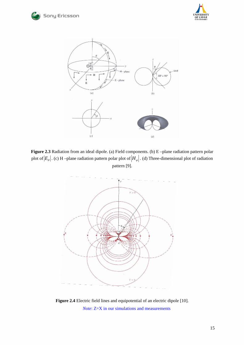
Figure 2.3 Radiation from an ideal dipole. (a) Field components. (b) E –plane radiation pattern polar plot of θE . (c) H –plane radiation pattern polar plot of ϕH . (d) Three-dimensional plot of radiation

pattern [9].

Figure 2.4 Electric field lines and equipotential of an electric dipole [10].

Note: Z=X in our simulations and measurements

15

After describing the field intensity now it is needed to find the relation between the radiated power

density and the field intensity and which is as follows:

2/)(21 mVAHES ×= 2.11

And the Equivalent isotropic radiated power [EIRP]

2.12 WdSP 24π×=

Where d is the distance from the antenna.

So to estimate the radiated power it is needed to measure the E and H field both. In this study a planar

measurement system is to be used with electric and magnetic field probes for measuring the E field

and H field respectively.

For measuring the H field components (Hx, Hy, Hz) the near field measurement system has two kinds

of probes one is horizontal and another is vertical one. Using those it is quite simple to measure the

entire three components. Where as measuring the E field components with electric field probe is

comparably difficult because of the placement of the probe antenna. The details about the

measurement system are described in next chapter.

So converting the magnetic field intensity to E field intensity the ERP can be calculated by using the

equation 2.11, 2.12 and 2.8. The conversion between the E and H field intensity is described by

Ω== 3770 HEZ 2.13

The equation 2.13 is based on the homogeneous far field condition i.e. the free space where is the

intrinsic impedance of free space.

0Z

16

Chapter 3

Measurement Setups

In this study we used two different measurement systems- HR1 near field Scanner and an outdoor far

field measurement system for FM frequencies with Optical fiber connection.

3.1 Near field measurement procedure design: 3.1.1 Setup for near field measurements with HR1 scanner:

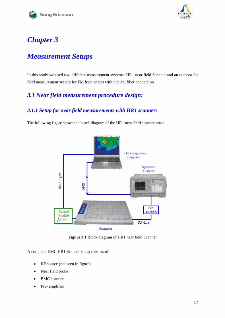
The following figure shows the block diagram of the HR1 near field scanner setup.

Figure 3.1 Block diagram of HR1 near field Scanner

A complete EMC HR1 Scanner setup consists of:

• RF source (not seen in figure)

• Near field probe

• EMC scanner

• Pre- amplifier

17

• Spectrum analyzer with GPIB (General Purpose Interface Bus) interface

• National instruments GPIB adapter

• Data acquisition computer with one RS-232 port

RF Signal Source:

The source provides the excitation to the DUT aperture (for passive measurement, active device like

mobile phone there is no need any RF source). The signal source must provide sufficient power to

insure an adequate signal to noise ration in the receiver. Higher power levels are required for higher

gain antennas due to the aperture mismatch loss between the probe and DUT. For this measurement

‘Rohde & Schwarz SMIQ03’ Signal Generator is used as the RF source.

Near Field Probe:

To perform with a near field analysis, we need to know how the E field and H fields are distributed.

The electric and magnetic probes are used to characterize the field distribution. Later on there is a

section which describes the probe principle and characteristic of electric and magnetic field probe

used in this study.

EMC scanner:

The planner scanner is required to accurately

position the probe antenna. The HR1 EMC scanner

which covers a 190x140x80 mm(X, Y, Z) region

with an accuracy of 0.05 mm is designed and

manufactured by Detectus AB. The HR1 EMC

scanner is shown in figure 4.8. For more details can

be found in reference [11]

Figure 3.2 EMC HR1 Scanner

18

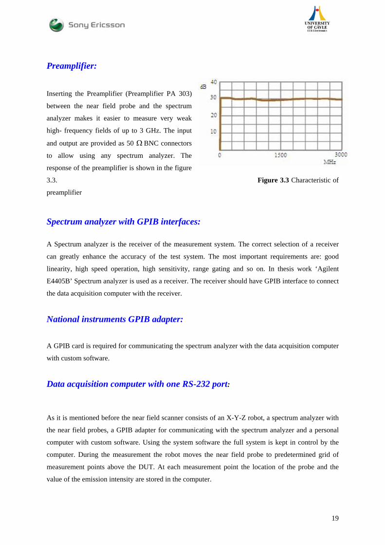
Preamplifier: Inserting the Preamplifier (Preamplifier PA 303)

between the near field probe and the spectrum

analyzer makes it easier to measure very weak

high- frequency fields of up to 3 GHz. The input

and output are provided as 50 ΩBNC connectors

to allow using any spectrum analyzer. The

response of the preamplifier is shown in the figure

3.3. Figure 3.3 Characteristic of

preamplifier

Spectrum analyzer with GPIB interfaces: A Spectrum analyzer is the receiver of the measurement system. The correct selection of a receiver

can greatly enhance the accuracy of the test system. The most important requirements are: good

linearity, high speed operation, high sensitivity, range gating and so on. In thesis work ‘Agilent

E4405B’ Spectrum analyzer is used as a receiver. The receiver should have GPIB interface to connect

the data acquisition computer with the receiver.

National instruments GPIB adapter:

A GPIB card is required for communicating the spectrum analyzer with the data acquisition computer

with custom software.

Data acquisition computer with one RS-232 port:

As it is mentioned before the near field scanner consists of an X-Y-Z robot, a spectrum analyzer with

the near field probes, a GPIB adapter for communicating with the spectrum analyzer and a personal

computer with custom software. Using the system software the full system is kept in control by the

computer. During the measurement the robot moves the near field probe to predetermined grid of

measurement points above the DUT. At each measurement point the location of the probe and the

value of the emission intensity are stored in the computer.

19

3.1.2 Near Field Probes Overview:

There are two types of EMC probes: Electric loop probe for E field and Magnetic loop probe for H

field measurement.

3.1.2.1 Property of the magnetic probe:

H field probe RS H 400-1: It has a diameter approximately 25 mm and is extremely sensitive and provides the average of the

magnetic field strength in the loop area of the probe. The probe is working effectively up to 10 cm

distance around modules and instruments.

(a) (b)

Figure 3.4 (a) magnetic field probe RS H 400-1 (b) gain

H field probe RS H 50-1:

Having a diameter approximately 10 mm it is higher in resolution and lower in sensitivity than the RS

H 400-1. It is suitable for performing measurements at a smaller distance of up to 3 cm (approx.). In

this range, the probe can determine the field distribution and field orientation even more precisely.

20

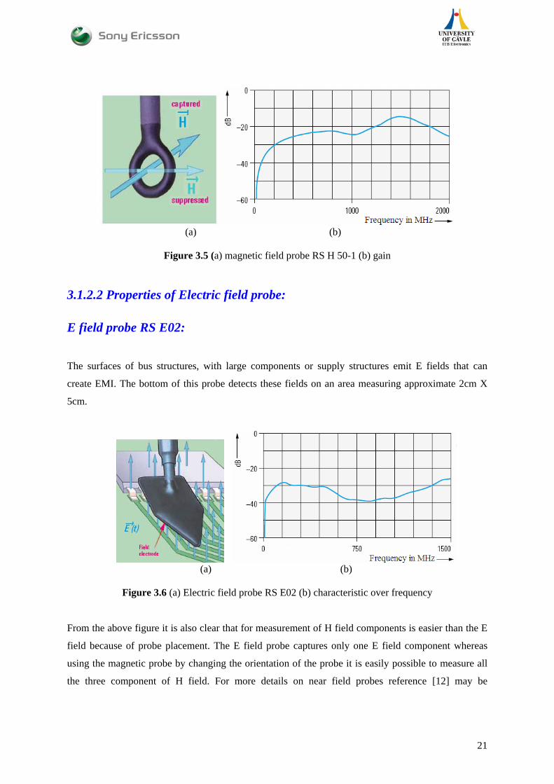
(a) (b)

Figure 3.5 (a) magnetic field probe RS H 50-1 (b) gain

3.1.2.2 Properties of Electric field probe:

E field probe RS E02:

The surfaces of bus structures, with large components or supply structures emit E fields that can

create EMI. The bottom of this probe detects these fields on an area measuring approximate 2cm X

5cm.

(a) (b)

Figure 3.6 (a) Electric field probe RS E02 (b) characteristic over frequency

From the above figure it is also clear that for measurement of H field components is easier than the E

field because of probe placement. The E field probe captures only one E field component whereas

using the magnetic probe by changing the orientation of the probe it is easily possible to measure all

the three component of H field. For more details on near field probes reference [12] may be

21

recommended. As in our study we will use the magnetic field probe then it is needed to know how the

magnetic probe works.

3.1.2.3 Basic Theory of Magnetic loop probes In Figure 3.7(a) a magnetic loop probe is shown. The equivalent circuit diagram is shown in Figure

3.7(b).

(a) (b)

Figure 3.7 (a) Shielded magnetic loop probe- unbalanced to the left, balanced to the right

and (b) equivalent circuit

The probes have shielded loops which reject the electric field and sample the magnetic field over a

small area. Only a short length of the loop conductor is exposed to the incident magnetic field. The

magnetic field passing through the probe loop generates a voltage according to Faraday’s low, which

states that the induced voltage is proportional to the rate of change of magnetic flux through a circular

loop.

(a) (b)

Figure 3.8 (a) HR1 scanner setup (b) The equivalent circuit (without amplifier)

22

So from the circuit Vind=Vl (i.c the load voltage is equal to induced voltage) From Faraday’s law the induced voltage is [13]

VoltsVABjV lind == ω 3.1 Where B is the magnetic flux density from the test antenna in Telsas

A= , is the area of probe loop in meter square,N is the number of turns of loop and r is the

radius of loop probe. Here N=1 (assumed).

22 rNπ

fπω 2= , is angular frequency in radians per second.

So from equation (3) magnetic flux to be found out and the magnetic field intencity H is given by

mABH /μ

= 3.2

Where μ is equal to H/m in free space. 7104 −×π

And then using equation (1) and (2) the radiated power can be estimated at far field region as at free

space

Ω== 3770 HEZ 3.3

The conversions are in Appendix B 3.2 Outdoors FF measurement system for FM frequencies with

Optical fiber connection: The main reason of using the far field measurement system for FM frequencies with optical fiber

connection is to improve the measurement result where the connection of a coaxial measurement

cable between the antenna and the measurement equipment is required. As this cable shielding is

metallic it has a large influence on the FM frequency measurement and prevents characterization of

the intrinsic properties of the antenna. This is especially true for small antennas (L < λ / 4). In order

to avoid the influence from cables during gain measurement, coaxial cable in measurement setup is

substituted by the optical fiber link.

Setup of the system Far field measurement system for FM frequencies with optical fiber connection consists:

23

• Transmitter with 50 Ohm RF input

• Optical fiber

• Receiver with 50 Ohm RF output

Figure 3.9 Fiber optics measurement systems

Transmitter, placed on PCB 100x40 mm, is about 55x40 mm size, and is fed by +3.7V. The

transmitter and receiver work in linear range, and convert modulated optical signal with modulation

depth proportional to the RF power. Signal Analyzer detects the RF signal (70-120 MHz) with the

power proportional to the received signal by antenna. Next, DUT is substituted by the reference

antenna with the known gain, and DUT gain is calculated.

Setup for Gain measurements

Figure 3.10 Measurement setup for measuring the gain of antennas by comparison For gain measurement we need the following equipments

• Signal Generator that operates in range at least between 70MHz to 120MHz.

• Signal Analyzer that operates in range at least between 70MHz to 120MHz.

• Two reference dipole antenna that operate in range at least between 70MHz to120MHz.

24

The absolute antenna gain is measured by comparing the received power between the reference dipole

antenna with known gain, and the DUT. The received power is measured in units of dBm

using a reference antenna with known gain . Utilizing the same experimental setup, the test

antenna replaces the reference antenna and the received power (dBm) is measured.

RG RP

RG

DP

The absolute gain of the measured antenna is thus given as: DG

)()()()( dBGdBmPdBmPdBG RRDD +−= 3.4

The gain measurement by comparison should be done with both antennas in a suitable location where

the wave from a distant source is substantially planed and has constant amplitude. There should also

be no multipath interference (MPI) from nearby objects.

For gain measurement the DUT is in the receiver site. And by knowing the antenna gain, EIRP and

the E field intensity can be calculated using the equations 2.7, 2.8 2.11 and 2.12.

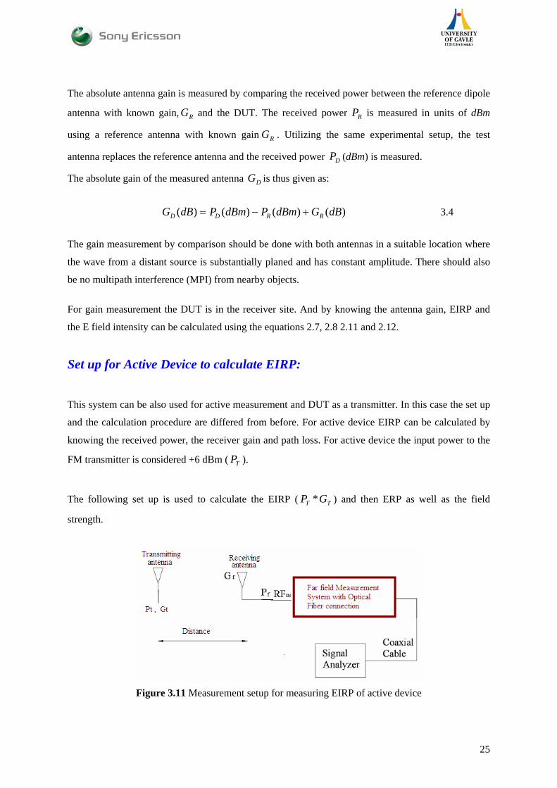
Set up for Active Device to calculate EIRP:

This system can be also used for active measurement and DUT as a transmitter. In this case the set up

and the calculation procedure are differed from before. For active device EIRP can be calculated by

knowing the received power, the receiver gain and path loss. For active device the input power to the

FM transmitter is considered +6 dBm ( ). TP

The following set up is used to calculate the EIRP ( ) and then ERP as well as the field

strength.

TT GP *

Figure 3.11 Measurement setup for measuring EIRP of active device

25

From the figure it is understandable that the well known free space equation is used here to account

for the path loss.

RTT

R GGPP 2

4⎟⎠⎞

⎜⎝⎛=πλ

3.5

In dB scale, PRTTR LGGPP +++= where )4log(20 πλ=PL

TG and is the transmitter and receiver gain and and is the transmitting and receiving

power. Here also using the 2.7, 2.10 and 2.11 the radiated power and the field strength are calculated.

RG TP RP

26

Chapter 4

Simulated Results

In this chapter the software simulations are going to be described. We use CST Microwave Studio

software to simulate the E(x, y, z) and H(x, y, z) field components distribution of a well known

reference antenna (DUT). Later on we will compare the simulated results with measured results of the

same reference antenna (DUT) to conduct with HR1 near-field scanner. Our reference DUT is a half

wave length sleeve dipole at resonant frequency. In addition one more DUT was used for comparison

which we define as basic FM-Transmitter phone model.

4.1 Simulation of half wave length dipole:

For measurement and simulation the reference antenna is 2/λ sleeve dipole at 880 MHz. One could

question why the reference antenna is 880 MHz dipole instead of 100 MHz (FM frequency). Two

main reasons can be mentioned. First, is the physical size limitation if we have to use a half wave

dipole antenna at 100 MHz which is 1.5 meter long. Second, reason is that the cable-fed FM devices

are difficult to handle at FM frequencies when it comes to cable decoupling and surrounding impact.

In our case most critical is the cable impact on the basic phone model FM antenna. The problem can

be partly solved by using balluns or ferrites but measurement repeatability and surrounding impact on

the antenna performance is still unreliable. In order to avoid the above mentioned problems we have

chosen to work at 880 MHz in this part of the study. Here one important statement need to present

that the input power which is used in simulation is 30 dBm. So all the simulated intensities and ERP is

respect to this input power.

(a) (b)

Figure 4.1 (a) Simulated 3D Geometry of Dipole antenna (b) Reference Dipole antenna

27

(a) (b)

(c) (d)

Figure 4.2: (a) and (c) simulated return loss and impedance

(b) and (d) measured return loss and impedance

From the above figures we saw that for both simulations model and the practical reference antenna

have the proper matching. After that we will see the pattern of the field strength at near field region.

28

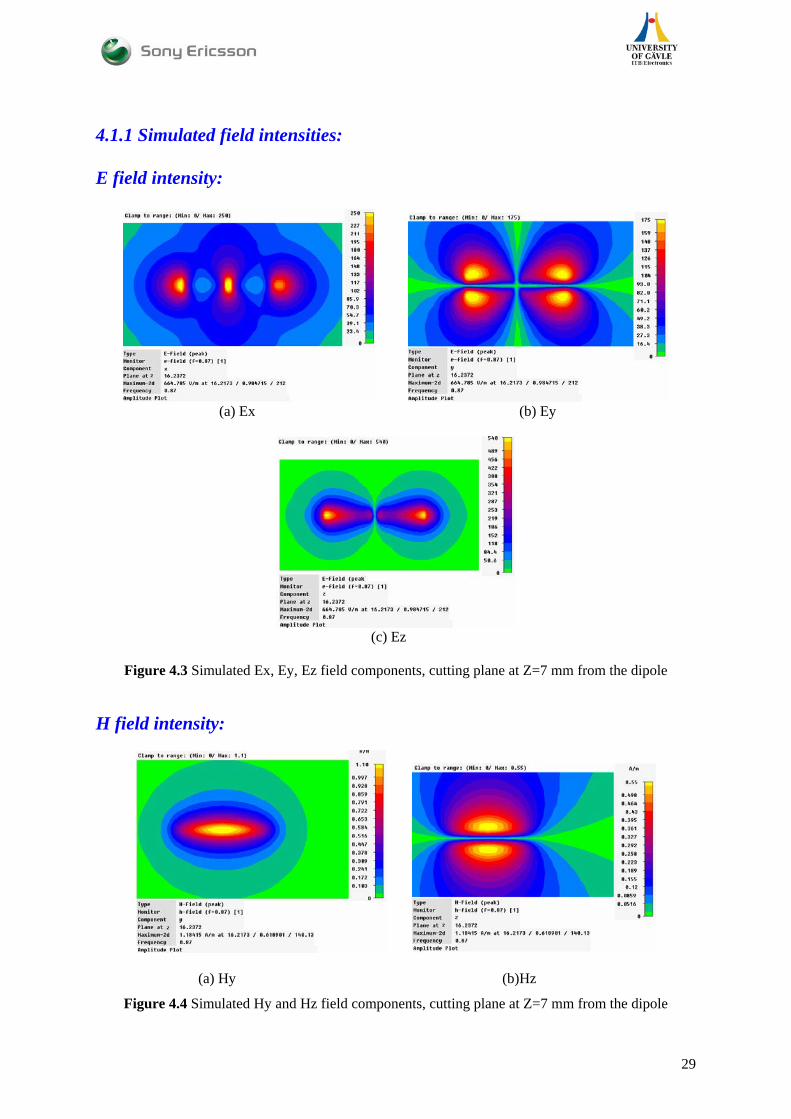
4.1.1 Simulated field intensities: E field intensity:

(a) Ex (b) Ey

(c) Ez

Figure 4.3 Simulated Ex, Ey, Ez field components, cutting plane at Z=7 mm from the dipole

H field intensity:

(a) Hy (b)Hz

Figure 4.4 Simulated Hy and Hz field components, cutting plane at Z=7 mm from the dipole

29

The figures show the E field and H field components i.e. Ex, Ey, Ez and Hy, Hz. From Figure 4.1 we

saw that the dipole is oriented along the X axis. The plots are taken at a certain distance above the

dipole along Z axis. In other words the plots are planes parallel to XY plane cutting Z axis in some

fixed distances.

From the figures above one can see that the E field components have quite complicated distribution

and therefore difficult to measure in practice. In the measurement point of view, the measurement of

E field components using the HR1 scanner is not convenient.

If we compare figure 2.4 and the simulated E field components we can see the following agreement:

Ex component has a field strength maximum at feeding point and at end of the dipole arms. For Ey

component 4 peaks can be observed whereas for Ez component there are two peaks as the components

are seen from a distance along Z axis.

Figure 2.3(c) shows the H field distribution which is like a close path around the dipole antenna.

Recalling figure 2.3 (c) there will be only two H field components Hy and Hz as the dipole is along X

axis in our simulations (Z axis from the plot is same as X axis in our simulations).

4.2 Simulation of Basic FM Transmitter Phone Model: The basic phone model is designed with PCB and a monopole antenna which can be used as a FM

transmitter. The size of monopole antenna is like typical one in mobile phone application.

Intentionally the antenna is made as less efficient at 100 MHz. Using the typical volume of this

antenna the resonance is found at 920 MHz which we will measure by near field scanner for the same

reason of using the dipole antenna. Further more, we will simulated this phone model at 100 MHz

which will give us the path loss which is needed to estimate the ERP and E field intensity at desired

distance for the FM transmitter.

4.2.1 Phone model at resonance frequency:

The PCB has typical mobile phone length of 100mm and the monopole antenna has a length that is

estimated to be good enough approximation for a FM Transmitter application. In addition to this the

phone model is optimized to be reasonably matched at 920 MHz, see Figure 4.6 below. This gives

measurement flexibility to our study.

30

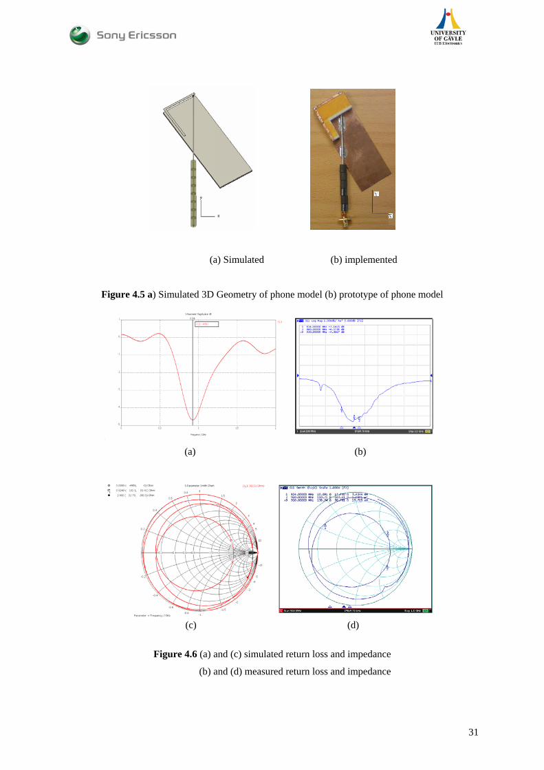
(a) Simulated (b) implemented

Figure 4.5 a) Simulated 3D Geometry of phone model (b) prototype of phone model

(a) (b)

(c) (d)

Figure 4.6 (a) and (c) simulated return loss and impedance

(b) and (d) measured return loss and impedance

31

4.2.1.1 Simulated Field intensities:

The following figures show the simulated E(x, y, z) and H(x, y, z) of the basic phone model at 920

MHz. All results are taken by cutting plane at Z=7 mm from the antenna surface.

E field intensity:

Figure 4.7 Simulated Ex, Ey, Ez field components, cutting plane at Z=7 mm from the phone model

H field intensity:

Figure 4.8 Simulated Hx, Hy and Hz field components cutting plane at Z=7 mm

from the phone model

The above figures are the 2D plots at X-Y plane like in the dipole case.

32

4.2.2 Phone model at FM frequency:

4.2.2.1 Simulated Field intensities: The field intensity is as follows using the same orientation of the model at previous section. The

distribution of the field intensity at 100 MHz as follows.

E field intensity:

Figure 4.9 Simulated Ex, Ey, Ez field components cutting plane at Z=7 mm

from the phone model

H field intensity:

Figure 4.10 Simulated Hx, Hy and Hz field components cutting plane at Z=7 mm

from the phone model

33

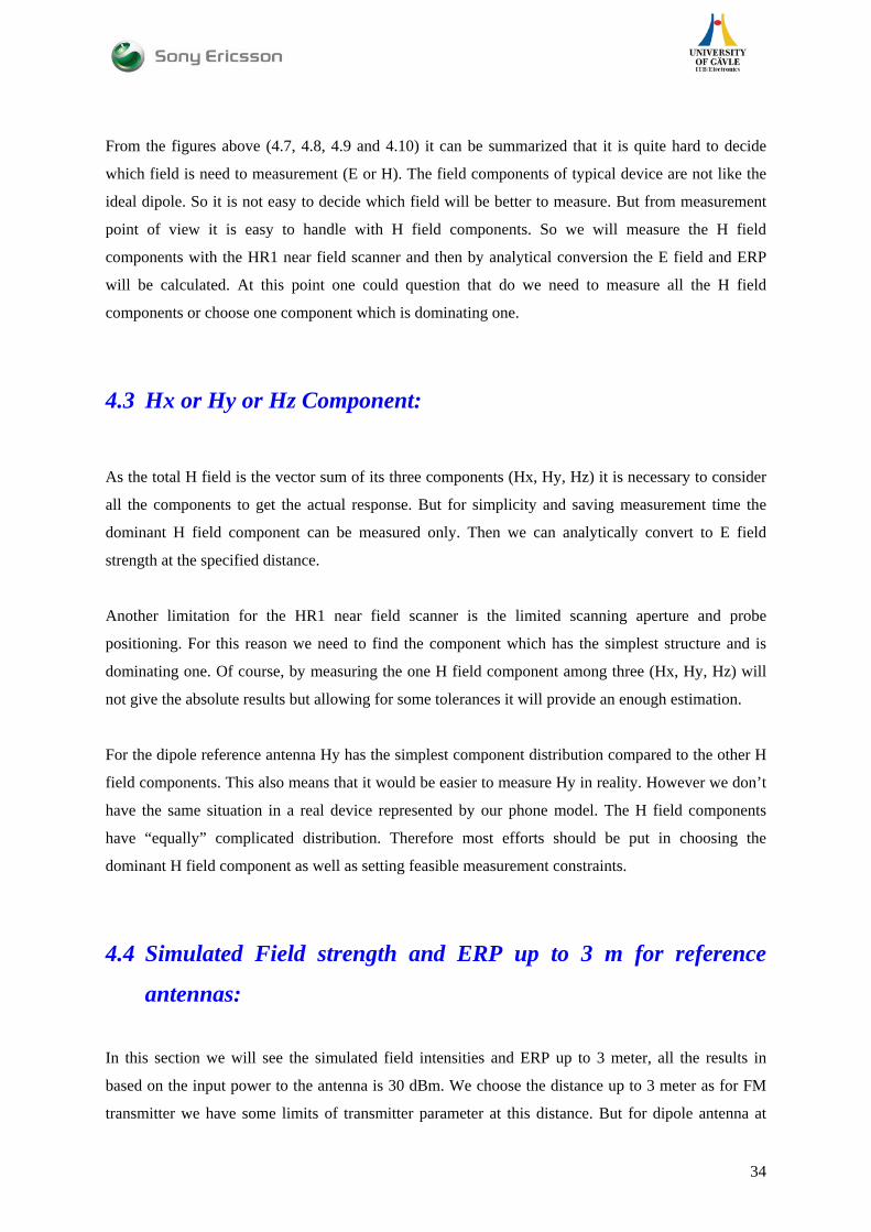
From the figures above (4.7, 4.8, 4.9 and 4.10) it can be summarized that it is quite hard to decide

which field is need to measurement (E or H). The field components of typical device are not like the

ideal dipole. So it is not easy to decide which field will be better to measure. But from measurement

point of view it is easy to handle with H field components. So we will measure the H field

components with the HR1 near field scanner and then by analytical conversion the E field and ERP

will be calculated. At this point one could question that do we need to measure all the H field

components or choose one component which is dominating one.

4.3 Hx or Hy or Hz Component:

As the total H field is the vector sum of its three components (Hx, Hy, Hz) it is necessary to consider

all the components to get the actual response. But for simplicity and saving measurement time the

dominant H field component can be measured only. Then we can analytically convert to E field

strength at the specified distance.

Another limitation for the HR1 near field scanner is the limited scanning aperture and probe

positioning. For this reason we need to find the component which has the simplest structure and is

dominating one. Of course, by measuring the one H field component among three (Hx, Hy, Hz) will

not give the absolute results but allowing for some tolerances it will provide an enough estimation.

For the dipole reference antenna Hy has the simplest component distribution compared to the other H

field components. This also means that it would be easier to measure Hy in reality. However we don’t

have the same situation in a real device represented by our phone model. The H field components

have “equally” complicated distribution. Therefore most efforts should be put in choosing the

dominant H field component as well as setting feasible measurement constraints.

4.4 Simulated Field strength and ERP up to 3 m for reference

antennas:

In this section we will see the simulated field intensities and ERP up to 3 meter, all the results in

based on the input power to the antenna is 30 dBm. We choose the distance up to 3 meter as for FM

transmitter we have some limits of transmitter parameter at this distance. But for dipole antenna at

34

880 MHz and the Phone model at 920 MHz it is not to require seeing simulated result up to 3 meter.

Actually our intention is to use one specific distance for all reference and test antenna. The following

figures show the simulated H and E field intensity, ERP up to 3 m for the three cases we have

simulated.

(a) Dipole (b) Phone model at 920

(c) Phone model at 100 MHz

Figure 4.12 Simulated field intensities and radiated power for dipole (a),

Phone model at 920 MHz (b) and phone model at 100 MHz

Now it needs to explain how we have drawn these curves from simulation. These plots are drawn

from the H field intensity. From chapter 2.2.2 and 2.2.3 which describe the field regions of antenna

size D<λ and D<<λ . Our reference antenna’s sizes are D< λ (for both 880 MHz and 920 MHz), so

35

equation 2.3 and 2.5 give are boundary of the near field and far field. Using these equations we got

the near field far field boundary for the dipole and phone model are 51 cm and 41 cm respectively. So

for plotting the field intensity first we use near field data up to the near field far field boundary from

the antenna surface then far field data are used . The antenna size of phone model at 100 MHz is

D<<λ . So for this case by using the equation 2.6 we got the boundary at 48 cm and we use the same

procedure to plot the field intensities and ERP up to 3 meter. From the above figures it is also shown

that the ERP of the radiated near field of the 3 simulated cases is not stable. As we know the field at

reactive near field is not stable it is like oscillating field. After the reactive near field boundary the

ERP is constant which is also meet the characterization of the effective radiated power by the antenna.

These simulated results will be used to compare with the measured result by the HR1 scanner. In

addition we will use these plots to define the path loss factor up to 3 m. If the measured result at a

certain distance from the object is equal to the simulated result then we can use the simulated path

loss factor in our calculation to estimate the field strength at 3 meter which will be shown in the next

chapter.

36

Chapter 5 Measurement Result In this study we measured reference dipole antenna and the basic phone model at 920 MHz and 100

MHz with HR1 scanner. First we measured the reference dipole antenna and the basic phone model at

920 MHz and estimated the ERP and E field intensity at 3 meter by using the measured and simulated

result. Then we made the validation of the HR1 scanner measurements by comparison with simulation.

And secondly, we measured the phone model at 100 MHz and estimated the ERP and field intensity at

3 meter by using the near field measurement result and simulation result and compared it to the

outdoor far field measurement result.

5.1 Reference Dipole antenna at 880 MHz:

5.1.1 Measured results

The measurement conditions for the dipole antenna are shown in figure 5.1

Figure 5.1 Measurement conditions of HR1 near field scanner for 880 MHz

37

The comparison between the measured and simulated result are done considering the following initial

conditions:

• The input power is 30 dBm for both simulation and measurement.

• The dipole is oriented along the x axis.

• The vertical loop probe is used for measurement which has -23 dB gain at 880 MHz.

• The measurement system has a 30dB amplifier and at 880 MHz the amplification is 25 dB.

But the values in the figures are the absolute results by compensated the probe gain as we

wanted to compare with the simulation results. That means the absolute field strength up to

specific distance from the antenna.

• All results are shown in dB scale to get better dynamic range.

• The Spectrum Analyzer gives the load power (50 Ohm) in dBm.

• Since the system is 50 Ohm then the load voltage can be calculated by converting the power.

Figure 3.8 shows in this measurement the load (50 ohm) voltage is equal to induced voltage

by the magnetic flux of the test antenna. For more details on voltage to field intensity

conversion Appendix A may be recommended.

• The same scanning area is considered for both simulations and measurements.

(a) Hz Setup (b) Hz measured (c)Hz simulated

(d) Hy Setup (e) Hy measured (f) Hy simulated Figure 5.2 Measurement of H field components of the dipole. (a) Orientation for Hz component. (b)

Measured Hz. (c) Simulated Hz. (d) orientation for Hy component.(e) Measured Hy.(f) Simulated Hy

38

The above figures make a sense that the near field scanner results and the simulated results are agree

each other very well. From the figures above it is also shown that the Hy component has higher

intensity and more simple distribution than Hz. So it could be convenient to measure the Hy

component as it has one peak position whereas for Hz it is two. Away from the antenna the Hz

component will be spread out which is difficult to measure because of the limitation of scanning area.

The following plots even better show that Hy component will be easier to measure and remains

unchanged when we move away from the DUT.

(a) Hy at 1 cm (b)Hy at 3 cm (c) Hy at 5 cm

(d) Hz at 1 cm (e) Hz at 3 cm (f) Hz at 5 cm

Figure 5.3 (a), (b) and (c) measured Hy component at 1, 3, 5 cm from the antenna.

(d), (e) and (f) measured Hz component at 1, 3, 5 cm from the antenna.

In the figures above 5.2 and 5.3 one important thing should be noticed that the scales are not the same.

The reason is in figure 5.3 the induced power by the dipole is directly shown in dBm whereas in

figure 5.2 this induced power is converted to the H field intensity in dBuA/m.

5.1.2 Estimation of field intensities and radiated power at 3 m distance:

The next step of comparison will be to estimate the E field intensity as well as the ERP at far field. As

for FM frequency the requirement is needed at 3 meter so for dipole and the phone model at 920 MHz

the distance is also taken at 3 meter. As the estimation of H field intensity is established based on

measurements placing the DUT at different distance from the probe of the scanner some general

conditions must be considered:

39

• The scanned are of the dipole is less than its full size as the physical length of it is large

compare to the scanner area. Furthermore, the highest strength is presents around the feeding

of the dipole antenna which are shown in figure 5.2 (e) and (f). So the area around the peak

position can be enough for measurement simplification.

• Three different approaches for scanning area have been used

The highest strength of the scanned area is dependent on the distance which is shown

in both measurement and simulation. So we peak the highest value of scanner area.

The average strength of the scanned area. We made an average of each point

measurement.

One specific position’s field strength. This position is that which gives the highest

field strength at initial measurement and also independent on distance.

Figure 5.4 Simulated and measured Hy component vs. distance

The ‘blue’ line shows the highest field strength of the scanned area, ‘black’ line is for the specific

position’s field strength of the area (Considering that position which gives the highest field by placing

the antenna very close to the probe), ‘green’ line for the average strength of the scanned area and last

of all the ‘red’ line is for the highest field strength in simulation. The latter has two sections first is up

to 50 cm where the near field data is used after that the far field data is used instead.

40

As the highest field strength is dependent on the distance so the measurement result of the ‘blue line’

could be consider to estimate the field strength and ERP at 3 meter. On the other hand the average

field strength is almost same varying the distance.

May be one can question why up to 50 cm the near field data is used. In chapter 4 we discuss shortly

but now we are describing it. This can be explained by the theory of field region of that antenna which

has the dimension D<λ . Bearing in mind the equation 2.3 and 2.5 the near field and far field region

boundaries can be calculated. For the dipole antenna, see section 2.3.2.

The Reactive near field boundary

cmmfCR 3434.0

10880103

6

8

1 ==××

=== λ

The ‘Fresnel’ region starts from

λλ +⎟⎟⎠

⎞⎜⎜⎝

⎛×=

223

2DDR =39 cm

Where D is the largest dimension of the antenna, here it is λ /2. The ‘Fresnel’ region stays up to radiating near field boundary. Actually the radiating near field starts

from the reactive near field boundary but from the Fresnel boundary it is more the radiation is more.

The radiating near field boundary or the inner radius of the far field is

λλ

+=2

32DR =51 cm

From equation 2.4 the outer radius of the radiating near field region is 51 cm. So up to this the near

field data is used then it shifted to far field data. Here it needs to mentioned that the near field data is

for one component (here Hy) but the far field data is given in spherical coordinate system so it

contains all the components. Earlier we have assumed that Hy is dominating so it can be also assumed

that at far field the Hy component also represents the total H field. From the simulated data it is found

that at distance of 51 cm from the antenna the far field and near field data is almost same. This proves

the boundary presence at this distance. Now it is time to estimate the field strength at 3m as well as

the radiated power.

41

Figure 5.5 The field region and H field intensity (simulated and measured)

From figure 5.5 it is shown that from 0 to 15 cm the simulated and the measured field is almost same

with a difference of ~17 dB, As 51 cm is the boundary for the near field the far field then it can be

taken as a reference point. For simulation the field strength is 90 dBuA/m where as for measurement

it is 117 dBuA/m. But the later result is not accurate as the probe can measure the field strength up to

3 cm precisely. So if we approximate the measured results with simulations the measured H field will

be 107 dBuA/m which is 17 dB higher than the simulation at 51 cm.

The following figure of simulated H field intensity up to 3 meter correspond to the near field and far

field data both which provide the path loss from 51 cm to 3 meter. We found the path loss is 15 dB.

Before we assumed that at 51 cm the measured H field intensity is 107 dBuA/m. So now using the

simulated path loss which is 15 dB from 51cm to 3 meter the estimated H field intensity at 3 meter

will be 92 dBuA/m ( 107- 15). And then using equation 2.8, 2.11 and 2.12 allows deriving E field,

EIRP and ERP shown in figure 5.6.

42

(a)

(b)

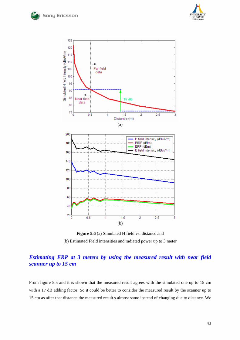
Figure 5.6 (a) Simulated H field vs. distance and

(b) Estimated Field intensities and radiated power up to 3 meter

Estimating ERP at 3 meters by using the measured result with near field scanner up to 15 cm From figure 5.5 and it is shown that the measured result agrees with the simulated one up to 15 cm

with a 17 dB adding factor. So it could be better to consider the measured result by the scanner up to

15 cm as after that distance the measured result s almost same instead of changing due to distance. We

43

used the measured H field strength up to 15 cm then using the simulated path loss from 15 cm to 3 m

we got the H field strength at 3 meter. In this case we were not considering the boundary.

At 15 cm the measured H field is 115.75 dBuA/m so using the simulated path loss from 15 cm to 3

meter we can estimate the H field at 3 meter which is 90.75 (115.75-25) dBuA/m. And then we can

analytically calculate the E field and ERP. This is shown below.

(a) (b)

Figure 5.7 (a) Simulated H field vs. distance and

(b) Estimated Field intensities and radiated power up to 3 meter

From the above figure it is shown that the results are almost same as in figure 5.6 (a)

5.1.3 Comparison between measured and simulated results: The tabular form of comparison between the simulated result and measured result is shown in table

5.1 and in figure 5.8.

Observations Simulated result Measured result (measured result up to 15 cm)

H field Intensity (dBuA/m) 75.735 90.75

E field Intensity (dBuV/m 127.24 142.25

EIRP (dBm) 29.023 44.288

ERP (dBm) 26.873 42.138

Table 5.1 Comparison the results at 3 meter from simulation to measurement

44

Figure 5.8 Comparison the results at 3 meter from simulation to measurement The simulated results are taken from the figure 4.12(a). 5.2 Phone model at 920 MHz: 5.2.1 Measured results: The same set up as for dipole antenna is considered for this measurement except the antenna

orientation and the frequency. In this case the model is placed along the y axis.

(a) Hx setup (b) measured Hx (c) simulated Hx

45

(d) Hy setup (e) measured Hy (f) simulated Hy

(g) Hz set up (h) measured Hz (i) simulated Hz

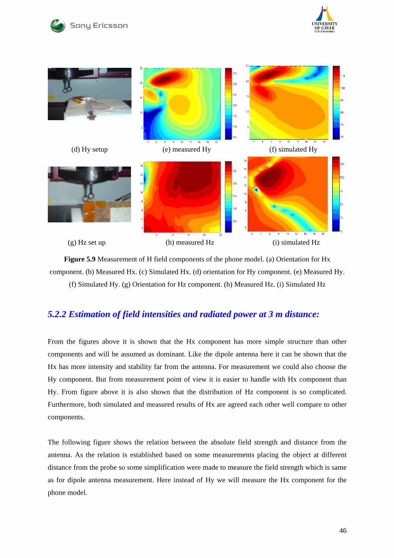
Figure 5.9 Measurement of H field components of the phone model. (a) Orientation for Hx

component. (b) Measured Hx. (c) Simulated Hx. (d) orientation for Hy component. (e) Measured Hy.

(f) Simulated Hy. (g) Orientation for Hz component. (h) Measured Hz. (i) Simulated Hz

5.2.2 Estimation of field intensities and radiated power at 3 m distance:

From the figures above it is shown that the Hx component has more simple structure than other

components and will be assumed as dominant. Like the dipole antenna here it can be shown that the

Hx has more intensity and stability far from the antenna. For measurement we could also choose the

Hy component. But from measurement point of view it is easier to handle with Hx component than

Hy. From figure above it is also shown that the distribution of Hz component is so complicated.

Furthermore, both simulated and measured results of Hx are agreed each other well compare to other

components.

The following figure shows the relation between the absolute field strength and distance from the

antenna. As the relation is established based on some measurements placing the object at different

distance from the probe so some simplification were made to measure the field strength which is same

as for dipole antenna measurement. Here instead of Hy we will measure the Hx component for the

phone model.

46

Figure 5.10 Simulated and measured Hx component vs. distance for the phone model

The ‘blue’ line shows the highest field strength of the scanned area, ‘black’ line is for the specific

position’s field strength of the area (Considering that position which gives the highest field by placing

the antenna very close to the probe), ‘green’ line for the average strength of the scanned area and last

of all the ‘red’ line is for the highest field strength in simulation. Here up to 41 cm the near field data

is used after that the far field data is used instead of near field.

As the highest field strength is dependent on the distance so the measurement result of the ‘blue line’

could be consider to estimate the field strength and ERP at 3 meter like the dipole measurement. On

the other hand the average field strength is almost same varying the distance.

We can explain the use of 41 cm which is the near field far field boundary for our phone model at 920

MHz. So like dipole our phone model dimension is D< λ (D =122 mm).

Using equation 2.3, 2.4 and 2.5 the field regions can be found. Reactive near field boundary

1R =32 cm The Fresnel region starts from

2R =35 cm The radiating near field boundary

3R =41 cm

47

So 41 cm is the boundary of near field and far field which will be the reference point for the phone

model to estimate the requirement.

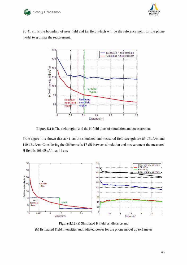
Figure 5.11: The field region and the H field plots of simulation and measurement

From figure it is shown that at 41 cm the simulated and measured field strength are 89 dBuA/m and

110 dBuA/m. Considering the difference is 17 dB between simulation and measurement the measured

H field is 106 dBuA/m at 41 cm.

Figure 5.12 (a) Simulated H field vs. distance and

(b) Estimated Field intensities and radiated power for the phone model up to 3 meter

48

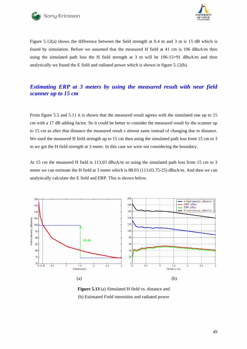
Figure 5.12(a) shows the difference between the field strength at 0.4 m and 3 m is 15 dB which is

found by simulation. Before we assumed that the measured H field at 41 cm is 106 dBuA/m then

using the simulated path loss the H field strength at 3 m will be 106-15=91 dBuA/m and then

analytically we found the E field and radiated power which is shown in figure 5.12(b).

Estimating ERP at 3 meters by using the measured result with near field scanner up to 15 cm

From figure 5.5 and 5.11 it is shown that the measured result agrees with the simulated one up to 15

cm with a 17 dB adding factor. So it could be better to consider the measured result by the scanner up

to 15 cm as after that distance the measured result s almost same instead of changing due to distance.

We used the measured H field strength up to 15 cm then using the simulated path loss from 15 cm to 3

m we got the H field strength at 3 meter. In this case we were not considering the boundary.

At 15 cm the measured H field is 113.03 dBuA/m so using the simulated path loss from 15 cm to 3

meter we can estimate the H field at 3 meter which is 88.03 (113.03.75-25) dBuA/m. And then we can

analytically calculate the E field and ERP. This is shown below.

(a) (b)

Figure 5.13 (a) Simulated H field vs. distance and

(b) Estimated Field intensities and radiated power

49

5.2.3 Comparison between measured and simulated results:

The tabular form of comparison between the simulated result and measured result from figure 5.12 is

shown in table 5.2 and in figure 5.14.

Observations Simulated result Measured result

H field Intensity (dBuA/m) 74.282 91.000

E field Intensity (dBuV/m 125.78 142.50

EIRP (dBm) 27.569 44.288

ERP (dBm) 25.419 43.138

Table 5.2 Comparison the results at 3 meter from simulation to measurement

Figure 5.14 Comparison the results at 3 meter from simulation to measurement

5.3 DUTs at 100MHz: In previous section we saw the measured estimated results of dipole reference antenna and the basic

phone model at 880 MHz and 920 MHz. Comparing the results from the scanner and the simulation it

is observed that the near field scanner measured the expected distribution of H field components have

a similar distribution but with a difference of 17~18 dB from the simulation. In this section the

50

measured results from the near field scanner of three test antennas will be described. The frequency is

100 MHz. The three test antennas are

• The basic phone model at 100 MHz

• Active device 1

• Active device 2

5.3.1 The basic Phone Model at 100 MHz:

5.3.1.1 Measured result:

Before describing the measured result it is needed to mention that the results from the scanner can be

erroneous as this is a passive (cable-fed) measurement where a coaxial cable is connecting the DUT

and the signal generator. Furthermore, we use ferrites to block the reversed current which may not be

so efficient at 100MHz.

To estimate the Field intensity and the radiated power at 3 m the following set up is used.

The RF source power is 6 dBm for measuring the H field intensity by the near field

scanner as for mobile phone the RF source is 6 dBm.

The frequency is 100 MHz instead of 880 MHz with the same measurement setup

as in figure 5.1

The same phone model which we used at 920 MHz. We assumed the Hx

component is dominating one for that frequency because of higher intensity and

simple distribution. But we cannot expect that the radiation pattern will be the same

for 920MHz and 100MHz.for same phone model. However we can say that we

assume Hx as dominant and will use it further in our 100MHz measurements.

The simulated H field intensity is used here only for getting the path loss slope.

For simulation the input power is 30 dBm.

In this chapter only measured results will be shown. Simulated H field intensity will

be used for making the path loss relation from a fixed distance to 3 meter.

51

Figure 5.15 Measured H field intensity vs. distance of phone model at 100 MHz.

5.3.1.2 Estimation of field intensity and radiated power at 3 meter:

The figure 5.16(a) shows the relation between the simulated H field intensity vs. distance. Up to 48

cm we used the near field data and then far field data is used. We considered 48 cm as the boundary

because for electrically small antenna (D<< λ ) at 100 MHz, the near field far field boundary is

πλ 2/≈R = 48 cm. More details can be found in chapter 2. From simulation we found that the path

loss from 48 cm to 3 meter is 15 dB.

(a) (b)

Figure 5.16 (a) measured H field intensity (b) Estimated field intensities

and radiated powers up to 3 meter.

52

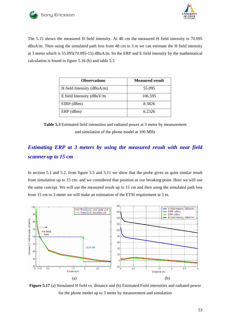
The 5.15 shows the measured H field intensity. At 48 cm the measured H field intensity is 70.095

dBuA/m. Then using the simulated path loss from 48 cm to 3 m we can estimate the H field intensity

at 3 meter which is 55.095(70.095-15) dBuA/m. So the ERP and E field intensity by the mathematical

calculation is found in figure 5.16 (b) and table 5.3

Observations Measured result

H field Intensity (dBuA/m) 55.095

E field Intensity (dBuV/m 106.595

EIRP (dBm) 8.3826

ERP (dBm) 6.2326

Table 5.3 Estimated field intensities and radiated power at 3 meter by measurement

and simulation of the phone model at 100 MHz

Estimating ERP at 3 meters by using the measured result with near field

scanner up to 15 cm

In section 5.1 and 5.2, from figure 5.5 and 5.11 we show that the probe gives us quite similar result

from simulation up to 15 cm. and we considered that position as our breaking point. Here we will use

the same concept. We will use the measured result up to 15 cm and then using the simulated path loss

from 15 cm to 3 meter we will make an estimation of the ETSI requirement at 3 m.

(a) (b)

Figure 5.17 (a) Simulated H field vs. distance and (b) Estimated Field intensities and radiated power

for the phone model up to 3 meter by measurement and simulation

53

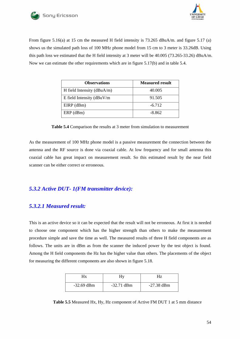
From figure 5.16(a) at 15 cm the measured H field intensity is 73.265 dBuA/m. and figure 5.17 (a)

shows us the simulated path loss of 100 MHz phone model from 15 cm to 3 meter is 33.26dB. Using

this path loss we estimated that the H field intensity at 3 meter will be 40.005 (73.265-33.26) dBuA/m.

Now we can estimate the other requirements which are in figure 5.17(b) and in table 5.4.

Observations Measured result

H field Intensity (dBuA/m) 40.005

E field Intensity (dBuV/m 91.505

EIRP (dBm) -6.712

ERP (dBm) -8.862

Table 5.4 Comparison the results at 3 meter from simulation to measurement As the measurement of 100 MHz phone model is a passive measurement the connection between the

antenna and the RF source is done via coaxial cable. At low frequency and for small antenna this

coaxial cable has great impact on measurement result. So this estimated result by the near field

scanner can be either correct or erroneous.

5.3.2 Active DUT- 1(FM transmitter device):

5.3.2.1 Measured result:

This is an active device so it can be expected that the result will not be erroneous. At first it is needed

to choose one component which has the higher strength than others to make the measurement

procedure simple and save the time as well. The measured results of three H field components are as

follows. The units are in dBm as from the scanner the induced power by the test object is found.

Among the H field components the Hz has the higher value than others. The placements of the object

for measuring the different components are also shown in figure 5.18.

Hx Hy Hz

-32.69 dBm -32.71 dBm -27.38 dBm

Table 5.5 Measured Hx, Hy, Hz component of Active FM DUT 1 at 5 mm distance

54

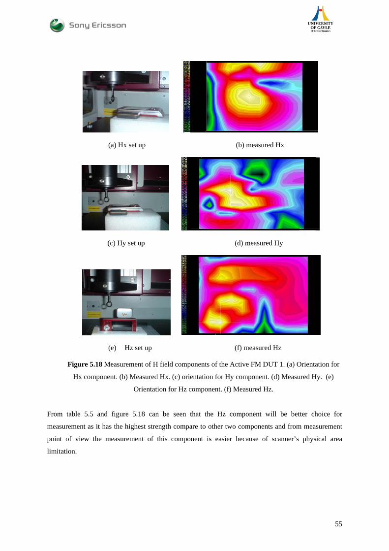
(a) Hx set up (b) measured Hx

(c) Hy set up (d) measured Hy

(e) Hz set up (f) measured Hz

Figure 5.18 Measurement of H field components of the Active FM DUT 1. (a) Orientation for

Hx component. (b) Measured Hx. (c) orientation for Hy component. (d) Measured Hy. (e)

Orientation for Hz component. (f) Measured Hz.

From table 5.5 and figure 5.18 can be seen that the Hz component will be better choice for

measurement as it has the highest strength compare to other two components and from measurement

point of view the measurement of this component is easier because of scanner’s physical area

limitation.

55

Figure 5.19 Measurement of H field of the Active FM DUT 1

5.3.2.2 Estimation of field intensity and radiated power at 3 meter:

The procedure of estimation of field strength and the radiated power is same as in section 5.3.1.2

which is describes the estimation of ETSI requirement of 100 MHz phone model at 3 meter. As we

saw in section 5.1 and 5.2 and 5.3.1.2 the measured result by the scanner is suited up to 15 cm from

the probe so here we will use the 15 cm as our measured reference point. For simplicity we will not

describe the estimation based on the near field far field boundary.

Figure 5.19 gives the measured H field intensity at 15 cm which is 63.76. So using the simulated path

loss from figure 5.16(a) we get the estimated H field at 3 meter which is 30.5( 63.76-33.26) dBuA/m

and the other requirement is placed in figure 5.20 and table 5.6 as follows:

Figure 5.20 Estimated Field intensities and radiated power for the Active DUT-1 up to 3 meter by the measured and simulated result.

56

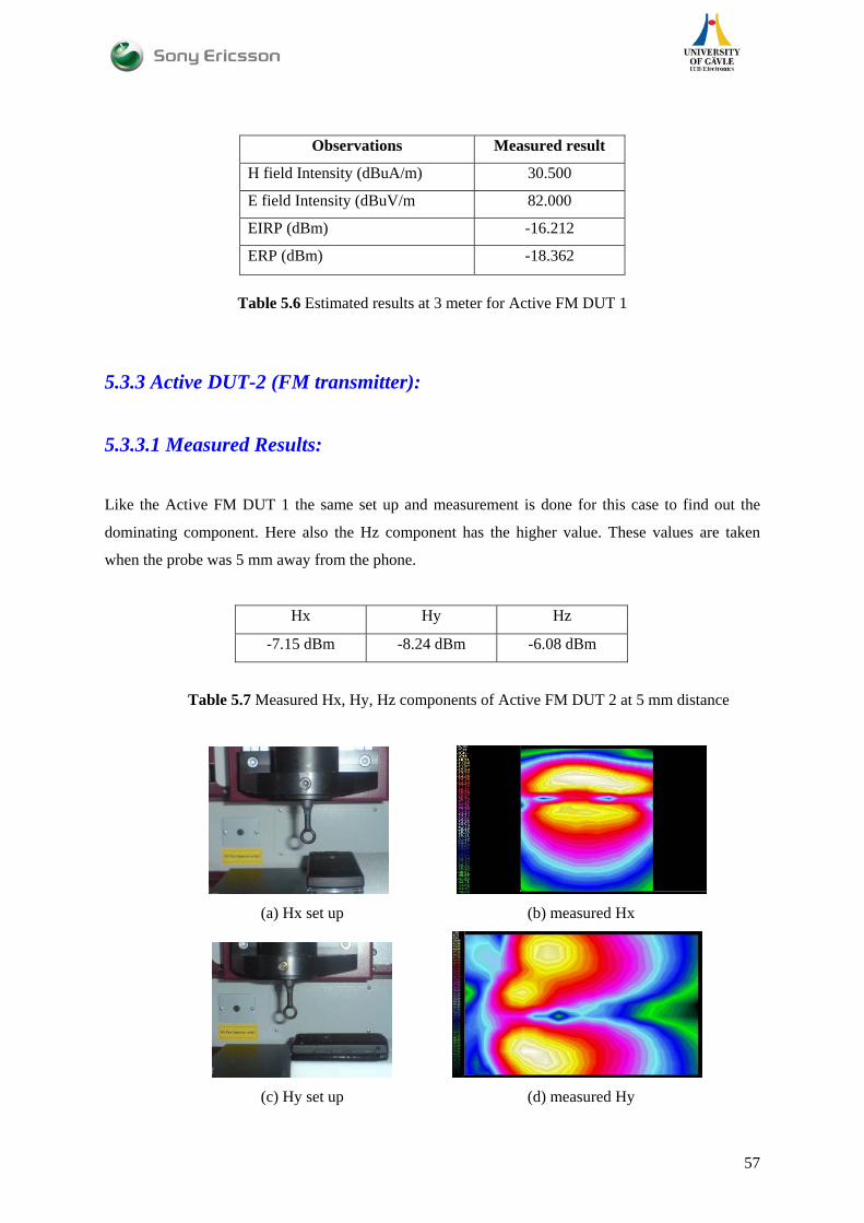
Observations Measured result

H field Intensity (dBuA/m) 30.500

E field Intensity (dBuV/m 82.000

EIRP (dBm) -16.212

ERP (dBm) -18.362

Table 5.6 Estimated results at 3 meter for Active FM DUT 1

5.3.3 Active DUT-2 (FM transmitter):

5.3.3.1 Measured Results:

Like the Active FM DUT 1 the same set up and measurement is done for this case to find out the

dominating component. Here also the Hz component has the higher value. These values are taken

when the probe was 5 mm away from the phone.

Hx Hy Hz

-7.15 dBm -8.24 dBm -6.08 dBm

Table 5.7 Measured Hx, Hy, Hz components of Active FM DUT 2 at 5 mm distance

(a) Hx set up (b) measured Hx

(c) Hy set up (d) measured Hy

57

(e) Hz set up (f) measured Hz

Figure 5.21 Measurement of H field components of the FM transmitter in a mobile phone. (a)

Orientation for Hx component. (b) Measured Hx. (c) orientation for Hy component. (d)

Measured Hy. (e) Orientation for Hz component. (f) Measured Hz.

Figure 5.21 Measurement of H field of the Active FM DUT 2

5.3.3.2 Estimation of field intensity and radiated power at 3 meter:

Like the active device 1 section 5.3.2.2, we simplified the measurement and estimation of the

requirements. We consider the reference point at 15 cm that means we will take measurement result

up to 15 cm then using the simulated path loss we will estimate ETSI requirement at 3 meter.

From figure 5.21 we get the measured H field intensity at 15 cm is 80.31 dBuA/m. So using the

simulated path loss at 100 MHz from figure 5.17 (a) which is 33.26 dB we get the H field intensity at

3 meter equal to 47.050 (80.31-33.26) dBuA/m. The ERP and the field intensities are plotted as

follows. Tabular form is in table 5.8 below.

58

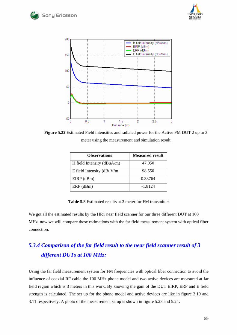
Figure 5.22 Estimated Field intensities and radiated power for the Active FM DUT 2 up to 3

meter using the measurement and simulation result

Observations Measured result

H field Intensity (dBuA/m) 47.050

E field Intensity (dBuV/m 98.550

EIRP (dBm) 0.33764

ERP (dBm) -1.8124

Table 5.8 Estimated results at 3 meter for FM transmitter

We got all the estimated results by the HR1 near field scanner for our three different DUT at 100

MHz. now we will compare these estimations with the far field measurement system with optical fiber

connection.

5.3.4 Comparison of the far field result to the near field scanner result of 3

different DUTs at 100 MHz:

Using the far field measurement system for FM frequencies with optical fiber connection to avoid the

influence of coaxial RF cable the 100 MHz phone model and two active devices are measured at far

field region which is 3 meters in this work. By knowing the gain of the DUT EIRP, ERP and E field

strength is calculated. The set up for the phone model and active devices are like in figure 3.10 and

3.11 respectively. A photo of the measurement setup is shown in figure 5.23 and 5.24.

59

Figure 5.23 Passive measurement

Figure 5.24 Active measurement

60

The estimated ERP and Field strength at 3 meter by the near field scanner is compared here with the

result of Far field measurement system. The optical connection is used indoors and outdoors to see the

effect of indoors reflections at FM frequencies. The results are also compared to those without the

fiber optic setup, where the reference antenna for the far field measurement is connected to the signal

analyzer directly via coaxial cable. The comparison is in table 5.9

* using the data up to 15 cm from the Scanner

100 MHz phone model Active FM DUT 1 Active FM DUT 2 Measurement

System EIRP (dBm)

ERP (dBm)

E field (dBuV/m)

EIRP (dBm)

ERP (dBm)

E field (dBuV/m)

EIRP (dBm)

ERP (dBm)

E field (dBuV/m)

Outdoor with OF -46.28 -48.43 51.96 -56.27 -58.42 41.97 -58.6 -60.75 39.64

Indoor with OF -50.50 -52.56 47.74 -55.5 -57.65 42.74 -53.3 -55.45 44.74

Outdoor with cable -42.30 -44.45 55.94 -54.30 -56.45 43.94 -56.81 -58.96 41.43

Near field Scanner* -6.712 -8.862 91.505 -16.212 -18.362 82.00 0.338 -1.813 98.55

Table 5.9 Comparison of the results of near field scanner and far field measurement of three DUTs

(the near field measurement results are taken from table 5.4, 5.6 and 5.8)

5.3.5 ‘1 Meter measurement’ and comparison with previous results:

In the previous section we have seen the measurement results for the 880 MHz dipole, basic phone

model at resonance frequency and also at 100 MHz and two active devices by the near field scanner.

We measured the three DUTs with far field measurement system with optical fiber connection at 3

meter and found there is a large discontinuity between the far field result and estimated result at 3

meter by using the near field scanner which is close to 40 dB. What could be the possible reason of

this discontinuity we will see later. But as we found some inaccuracy of the near field measurement

system then may be it could be better to suggest a simple system for the characterization of FM

transmitter. In previous section we consider the measurement result from the near field scanner at 15

cm and predict the requirement at 3 meter by using the simulation results. As we discussed before for

small antenna at 100 MHz near field far field boundary is at 48 cm but we took our measurement

61

result at 15 cm which is in reactive near field region. This could be one possible region for getting the

inaccuracy in measurement result as we know that at reactive near field the fields are not stable.

So we can measure our DUTs at 1 m which will provide us the measured result close to reactive near

field and with this result we can easily predict our requirement at 3 meter by using the simulation

result like before. This measurement provide us compact, stable measurement and also with less

diffraction.

Here we are approaching a very simple measurement system for which we need only one 100 MHz

reference dipole antenna and a signal analyzer which detects the RF signal (100 MHz) with the power

proportional to the received signal. Our DUTs will be in transmitting mode. The set up can be

explained by the following figure:

Figure 5.25: The new measurement system setup

We made numbers of measurement by rotating the DUTs for getting the EIRP with both horizontal

and vertical polarizations. To calculate the EIRP we used the same equation 3.5 which is well known

free space equation. And then we converted the EIRP to E field intensity at 1 meter and as a

consequence we used the path gain from 1 meter to 3 meter from the simulation technique. The

reference dipole antenna is the tuned dipole one with the frequency range of 65 MHz to 180 MHz.

The technical information (dipole length, gain) is found in appendix D and also in reference [14].

Using this measurement we got the results which is going to compare with previous result using the

near field scanner and outdoor FF measurement with optical connection.

62

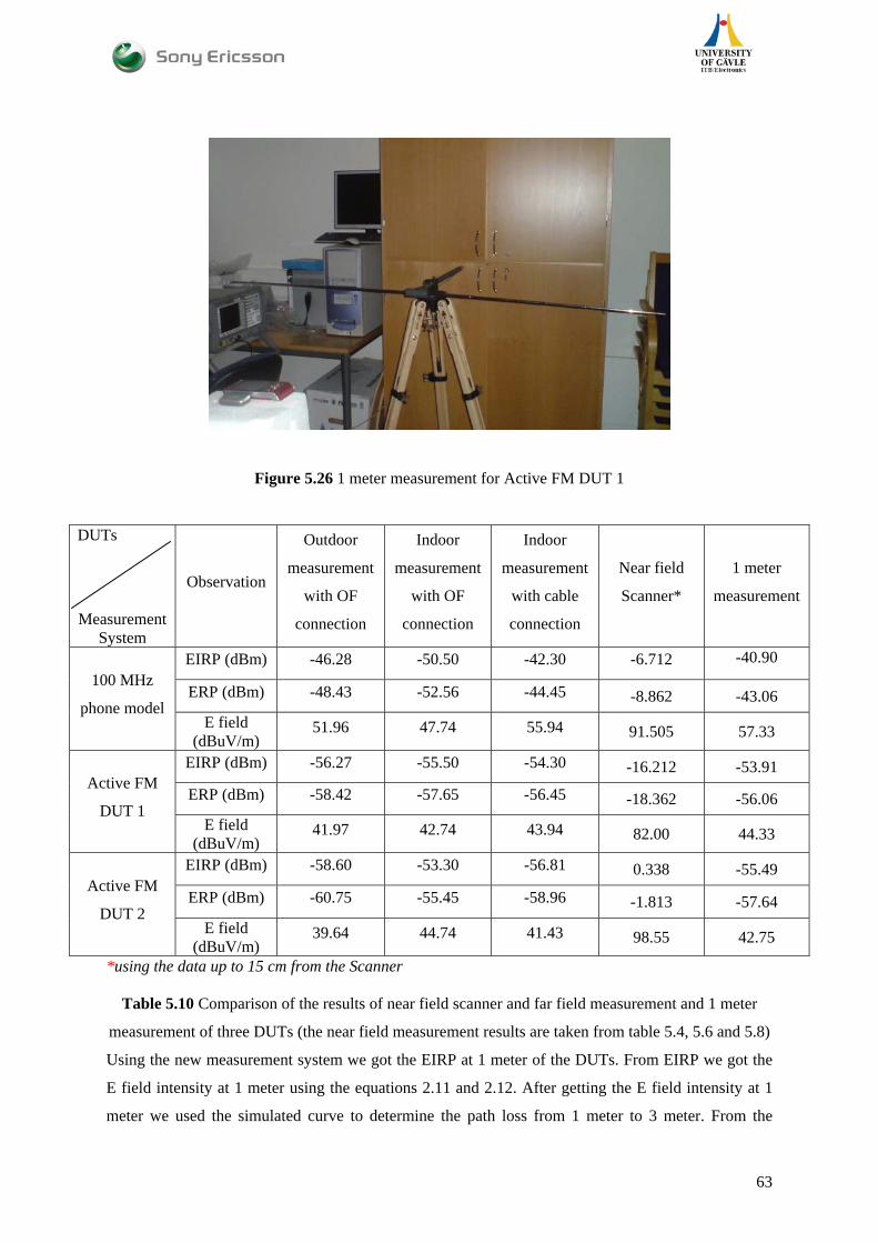
Figure 5.26 1 meter measurement for Active FM DUT 1

DUTs

Measurement

System

Observation

Outdoor

measurement

with OF

connection

Indoor

measurement

with OF

connection

Indoor

measurement

with cable

connection

Near field

Scanner*

1 meter

measurement

EIRP (dBm) -46.28 -50.50 -42.30 -6.712 -40.90

ERP (dBm) -48.43 -52.56 -44.45 -8.862 -43.06 100 MHz

phone model E field

(dBuV/m) 51.96 47.74 55.94 91.505 57.33

EIRP (dBm) -56.27 -55.50 -54.30 -16.212 -53.91

ERP (dBm) -58.42 -57.65 -56.45 -18.362 -56.06 Active FM

DUT 1 E field

(dBuV/m) 41.97 42.74 43.94 82.00 44.33

EIRP (dBm) -58.60 -53.30 -56.81 0.338 -55.49

ERP (dBm) -60.75 -55.45 -58.96 -1.813 -57.64 Active FM

DUT 2 E field

(dBuV/m) 39.64 44.74 41.43 98.55 42.75

*using the data up to 15 cm from the Scanner

Table 5.10 Comparison of the results of near field scanner and far field measurement and 1 meter

measurement of three DUTs (the near field measurement results are taken from table 5.4, 5.6 and 5.8)

Using the new measurement system we got the EIRP at 1 meter of the DUTs. From EIRP we got the

E field intensity at 1 meter using the equations 2.11 and 2.12. After getting the E field intensity at 1

meter we used the simulated curve to determine the path loss from 1 meter to 3 meter. From the

63

following figure it is shown that the simulated path loss from 1 meter to 3 meter for 100 MHz phone

model is 10 dB.

Figure 5.27 Simulated path loss of the 100 MHz phone model from 1 meter to 3 meter

Now we can find the E field intensity at 3 m which will be 10 dB lower than the E field intensity at 1

meter. Then using this field intensity at 3 meter we can easily calculate the EIRP and ERP at 3 meter

by the equations 2.11 and 2.12. The calculated results for the 3 DUTs are tabulated in table 5.10 in

column 7.

The comparisons between the measured results by different measurement system are shown in figure

5.28.

64

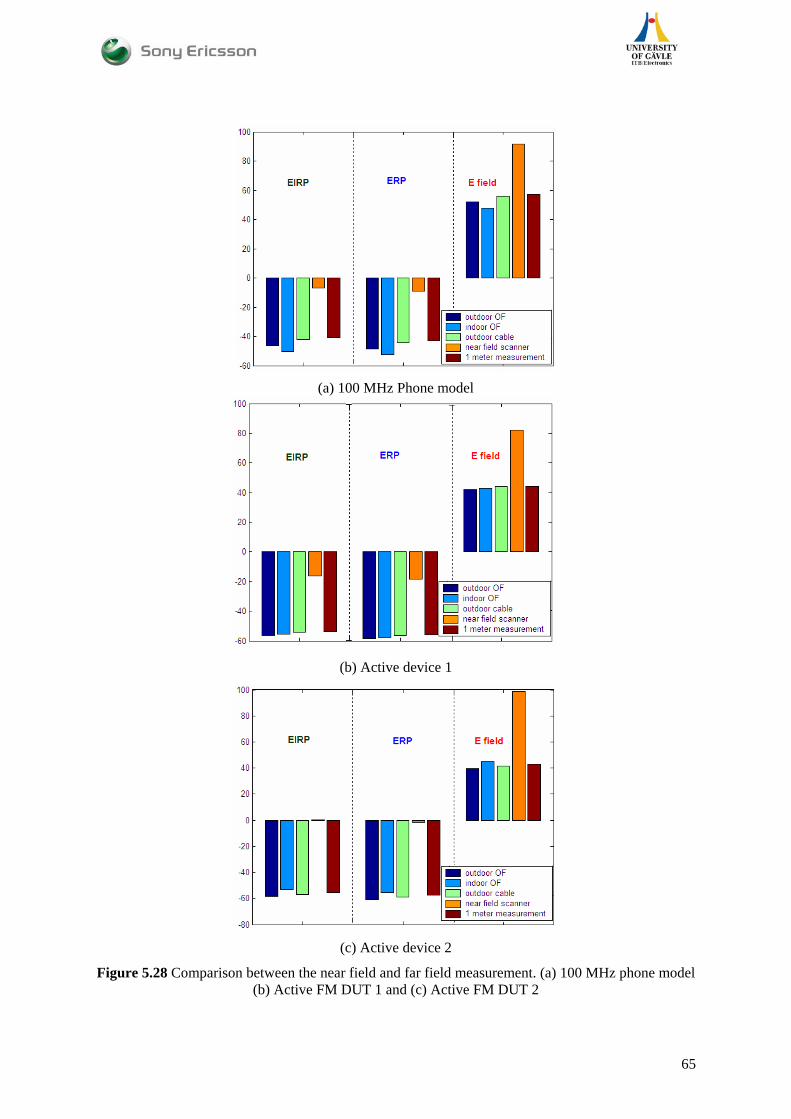
(a) 100 MHz Phone model

(b) Active device 1

(c) Active device 2

Figure 5.28 Comparison between the near field and far field measurement. (a) 100 MHz phone model (b) Active FM DUT 1 and (c) Active FM DUT 2

65

Now we can make some conclusion on the simulated and the measurement result for the reference

antenna and also for measurement results by the near field, far field measurement and as well as 1

meter measurement system of three DUTs.

From the table 5.1 and 5.2 it is shown that there is a quite high difference (17~18 dB) between the

simulated and measured result for the reference antenna. This unexpected difference can be explained

in the following way.

• It is mentioned in chapter 2 how does the near field probe work. From the spectrum analyzer

the measured outcomes are in dBm which is the induced power by the DUT. After some

mathematical calculation the H field intensity is found using equation 3.1 and 3.2. These two

equations are based on voltage unit but as the measurement system is in 50 ohm so it is very

convenient to convert from power to voltage. But a problem is raised using the equation 3.2

which state thatμBH = . In free space the value of μ is mH / . But as it is in near

field location it is not free space. The basic electromagnetic says that

104 7−×π

HB m )1(0 χμ +=

HHr μμμ == 0 (Wb/m ) 2

Or μBH = (A/m)

Where 0

1μμχμ =+= mr

is the dimensionless quantity known as relative permeability of the medium. The parameter

rμμμ 0= is the absolute permeability of the medium. The permeability of most materials is

very close to that of free space ( 0μ ) that means rμ is close to 1. But for the ferromagnetic

materials it could be very large number. And for both dipole and the phone model the ferrite

are used. But the permeability of the medium is not only depend on the ferrite as there are a

lot of materials present beside the DUT as the scanner is made of some metal substances. In

this thesis paper for the mathematical calculation the permeability of free space is used

because of simplicity which can be the reason for making the difference between the

simulation and measured result.

66

• Another reason can be the reflection from the scanner table. As the placement of the probe

and the scanner table is close to each other then the DUT is placed not so far from the scanner

table. As a result some reflection from the scanner table and well can be affected the

measured result.

• The measurement is taken in reactive near field region which can give erroneous result since

the reactive near field regions are not as “stable” where as they are in far field region.

• Another limitation is that the probe is sensitive up to 3 cm according to specification and the

dynamic range is 40 dB. During measurement it is shown quite similar result up to 15 cm. So

it is not possible to measure the field intensity at radiated near field zone as well as the far

field for around 900 MHz antennas.

Figure 5.28 (a) shows the comparison between the near field measurement, far field measurement and

1 meter measurement for 100 MHz phone model. Like the dipole and the phone model at 920 MHz

some difference in near field and far field measurement with optical fiber connection also seen here.

The difference from the estimated result from the scanner is overestimated by ~40 dB which is quite

large to compare with the reference antenna measurement which was ~17 dB between the simulation

and measurement. But our new technique of measurement to find out the requirements of FM

transmitter at 3 meter is showing quite good approximations for 100 MHz phone model which is

shown in figure 5.27 (a) and also in table 5.10. So, this is very interesting to see that the results using

the 1 meter measurement and the far field measurement system is conduct each other in very good

way.

Figure 5.28(b) shows the comparison for the Active FM DUT 1. Like 100 MHz phone model here the

estimated results by the near field scanner is ~40 dB above from the far field measurement. But the 1

meter measurement and the FF measurement gives the quite same results.

Figure 5.28 (c) shows the comparison for the Active FM DUT 2. Undesirably the difference between

the results by FF measurement and the near field measurement system is higher then the other two

cases. For this case the difference is ~58 dB. This is totally unexpected. Actually during the near field

measurement this transmitter gives 18 dB higher values than the Active FM DUT 1 whereas in far

field measurement it is almost similar to Active FM DUT 1 result. In the mobile phone this FM

transmitter antenna is also applicable for FM receiver. At near field may be there is some undesirable

radiations by the antenna which can be influence the results. As like other two cases the 1 meter

measurement gives us good approximation than the near field measurement system.

67

From the comparison between the simulation and the near field scanner result of the reference antenna

we expected that for 100 MHz FM transmitter the difference between the near field measurement and

far field measurement will be close to ~20 dB (for reference antenna it was ~18 dB) but table 5.9 and

5.10 and figure 5.28 show an unexpected difference between them which is ~40 dB. The possible

reasons will be discussed in chapter 6.

68

Chapter 6 Discussions

6.1 Measurement System feasibility:

In this thesis work the intention was to use two measurement systems - HR1 near field Scanner and

outdoor far field measurement system with optical fiber connection. In addition we introduced another

measurement method which we said as ‘1 meter measurement’. Actually all of them have some

advantages and some limitations. These limitations have to be considered while measurement is to be

done with them.

6.1.1 HR1 near field scanner: From the specification of HR1 scanner the dimensions are 190x140x80 mm (X, Y, X). This is quite

small space for measuring low frequency devices, especially if the measurement is required in

radiating near field region. As a result the measurement of H field intensity is done outside the

scanner table. For this reason the H field probe is better choice than E field probe as the orientation of

the E field probe is such that it is needed to place DUT upon the scanner table and then it will be not

possible to measure the E field more than 80 mm (Z axis) distance from the scanner table.

H field magnetic probe which is used to measure the magnetic field intensity has some drawbacks

also. This probe is sensitive up to approximately 3 cm which is relatively low for measuring a low

frequency device as this distance is in the reactive field region. But in the time of measurement it is

observed that up to 15 cm the measurement result is similar to the simulation (chapter 5). Another

limitation is analyzed that the probe’s dynamic range is 40 dB. As a result, while measuring the FM

transmitter which is a “poor” antenna (-40 to -50 dB gain) at 100 MHz the scanner is not able to

measure the actual field strength. For 100 MHz small antenna, 15 cm distance from the probe which

we take the reference measurement point is really in the reactive near field region. The E field

intensity is decaying so swiftly with the increase of distance which was shown in figure 5.15, 5.19 and

5.21. At 15 cm we should get lower value than the measured result. Because of 40 dB dynamic range

the proper result is not found. So this probe is not well suited for measurement of field strength of low

efficient antenna like FM transmitter with FM band. In the case of using the HR1 scanner for 100

69

MHz it could provide a better result if the reference point for the measurement is taken at closer

distance from the probe.

6.1.2 Outdoor Far field measurement system with optical fiber connection:

The far field measurement system with optical fiber connection is used to make a feasible relationship

between the absolute field strength and measured power in order to correlate the near field scan

results and far field measurement. The test setup for the active and passive measurement is shown in

figure 3.10 and 3.11 respectively. For passive measurement the DUT acts as a receiver whereas for

active measurement it is a transmitter.

There is some limitation for measuring the DUT as a transmitter. From the parameter table

(Appendix C) of far the field measurement system it is shown that the measurement range for input

power to the receiver optical fiber connection is -70 to -20 dBm. So for passive measurement this

range of input power should be maintained.

6.1.3 ‘1 meter measurement system’:

In previous chapter we described a new measurement system with a reference antenna which is

experimentally tuned dipole antenna (65 MHz to 180 MHz). From the calibration data sheet at 1 meter

calibration of this antenna we got the behaviors of it at 100 MHz. We measured the EIRP of our

DUTs at 1 meter and converted it to E field intensity at 1 meter. After that we estimate the E field

intensity at 3 meter by using the simulated path loss. Using this measurement system we got more

similar result to the FF measurement with the optical fiber connection. As a consequence we can say

this measurement gives more reliable result rather than the estimated results by the near field

measurement.

To calculate the EIRP of the DUTs we use the Friis equation. May be one could ask if this equation is

applicable for such a distance (1 meter) as we know there are some conditions for using the free space

equation which can be found in reference [7,8]. However in this case we use free space equation for

getting the path loss of 1 meter. But there is one good paper reference [15] which described very well

how to calculate the path loss for electrically small antenna at near field region. Using that process the

path loss is almost same by using the free space. So it can be concluded that we can easily use the free

space equation for getting the path loss as well as the EIRP of the DUTs. As a result we can strongly

70

say that this measurement will be the better choice to estimate the requirement for the FM transmitter

at 3 meter.

6.2 Measurement of reference antennas using HR1 near field scanner:

The measurement has been performed in HR1 near field scanner using the vertical magnetic field

probe which has introduced some unexpected uncertainty in results for that has been simulated. These

have to be considered when the estimation of ERP will be done at desired distance. In this thesis the

half wave length sleeve dipole antenna is used at 880 MHz and basic phone model at 920 MHz. The

measured results are shown in figure 5.6 and 5.10 for dipole and phone model respectively which are

followed the simulated result but with a additional factor of 17~18 dB. Although the probable reasons

for that difference between the simulation and measurement are described in chapter 5, it is mentioned

here again on brief.

• The entire calculation procedure is done by considering the permeability of free space. But in

practice the area very close to the DUT is not free space. If the actual permeability at near

field would be used then this inconsistency may not arrived.

• The result can be influenced by the reflection of the scanner table.

• The estimation of the field intensity as well as ERP is done on the basis on reactive near field

measurement. As it is known that the field pattern at this region is not stable so the result can

be erroneous.

6.2.1 Measurement of DUTs using HR1 near field scanner: The estimated ERP and field strength at 3 meter of the three DUTs are shown in table 5.4, 5.6 and 5.8.

By analysing the result in table 5.5 and 5.7 for the active device it is seen that there is some conflict

between the measured results of these two devices. Both devices are measured at 5 mm away from the

device. There is approximately 18 dB difference between the two measurement results. And this 18

dB difference also found at 3 meter. But using the outdoor far field measurement system with optical

fiber connection the measured results for the two devices are almost same which is shown in table 5.9

and 5.10. This results shows how sensitive is to measure in nearfield regions where the reactive

energy is dominant compared to the radiated. The different antenna types would create different

reactive nearfield which is difficult to compare

71

72

Chapter 7

Conclusion and Future Research 7.1 Conclusion:

The main goal with this thesis is to characterize a mobile phone FM transmitter device by Nearfield

measurements with 2D scanning equipment. First we did a validation of the Nearfield scanner by

simulations and measurements of reference antennas where we compare the results. Secondly, a

number of DUTs were measured in the near field scanner and with an outdoor far field range to

compare the results. At the end the total measurement procedure can be summarized by the following

equation to estimate the field strength and as well as the ERP of the FM transmitter at 3 meter.

V= P1+8+107-120 dBV

=)/(3 mdBuVEfield + +

2 3

Measured result from HR1 scanner at 15 cm,

P1 (dBm) 107-120dB 8 dB

1

+ - + + … 7.1

4 5 6 7

33.26dB

51.5 dB

-40 dB V-(-146.1346)-2

=)(3 dBmERPπ

π

1202

3410.10 2

2

6203

×

⎟⎟⎠

⎞⎜⎜⎝

⎛ −E

7.2

The calculations of the block 3, 4 and 6 are placed in Appendix B. In block 2, this 8 dB is the

compensated factor to minimize the probe gain in the measurement and in block 5, 33.26 is the path

loss.

In short, the description of equation 7.1 is as follows:

73

• Block 2 presents the terms which is a compensation factor to minimize the probe gain in the

measurement.

• Block 3 presents the conversion from dBm to dBuV.

• Block 4 presents the conversion from dBuV to dBpT (factor -146.1346) and from dBpT to

dBuA/m (factor 2).

• Block 5 presents the pathloss term from 15 cm to 3 m which is simulated.

• Block 6 presents the conversion from dBuA/m to dBuV/m.

• Block 7 presents the unknown measurement uncertainty which we found by comparing the

near field and far field measurement result.

Equation 7.2 is follows the equation 2.11 and 2.12 in dB scale.

So, the total measurement procedure will be done using the above equations. Using these equations

the following figure can be plotted which will give us a relation between the induced power by the

test antenna from the scanner (dBm) at 15 cm and the E field (also ERP) at 3 m.

(a) E field (b) ERP

Figure 7.1: (a) relation between the scanner result at 15 cm and estimated E field intensity at 3 meter

(b) relation between the scanner result at 15 cm and estimated ERP at 3 meter

Using this curve we can easily determine the ERP and E field intensity at 3 meter. In chapter 5

(section 5.3.5) we described the ‘1 meter measurement’ which gives us more reliable result at 3 meter.

In this case we do not need to consider any unknown measurement uncertainty factor like near field

measurement system (equation 7.1, block 7).

74

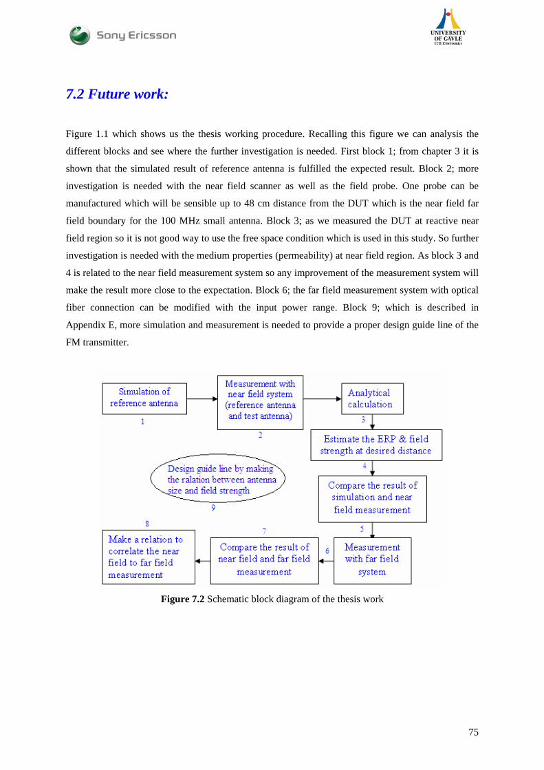
7.2 Future work:

Figure 1.1 which shows us the thesis working procedure. Recalling this figure we can analysis the

different blocks and see where the further investigation is needed. First block 1; from chapter 3 it is

shown that the simulated result of reference antenna is fulfilled the expected result. Block 2; more

investigation is needed with the near field scanner as well as the field probe. One probe can be

manufactured which will be sensible up to 48 cm distance from the DUT which is the near field far

field boundary for the 100 MHz small antenna. Block 3; as we measured the DUT at reactive near

field region so it is not good way to use the free space condition which is used in this study. So further

investigation is needed with the medium properties (permeability) at near field region. As block 3 and

4 is related to the near field measurement system so any improvement of the measurement system will

make the result more close to the expectation. Block 6; the far field measurement system with optical

fiber connection can be modified with the input power range. Block 9; which is described in

Appendix E, more simulation and measurement is needed to provide a proper design guide line of the

FM transmitter.

Figure 7.2 Schematic block diagram of the thesis work

75

76

References [1] Draft ETSI EN 301 357-1 V1.4.1 (2007-12), “Electromagnetic compatibility and Radio

spectrum Matters (ERM); Cordless audio devices in the range 25 MHz to 2000 MHz; Part 1

Technical characteristics and test methods”. www.etsi.org.

[2] FCC standards, “Part 15- Radio frequency devices”, section 15.239, pp 84-85, January 2001.

[3] Arthur D. Yaghjian, “An Overview of Near- Field Antenna Measurements”, IEEE Transactions

on Antennas and Propagation, vol.34, no.1, pp 30-33, January 1986.

[4] NSI, “Antenna Measurement Solutions”, 2001.

[5] James Mclean, Robert Sutton and Rob Hoffman, “Interpreting Antenna Performance Parameters

for EMC Applications- Part 2”, www.djmelectronics.com.

[6] Tom Lecklider, “The world of the Near Field: when Scotty is beaming up, he's working in the

very far field”, EE-Evaluation Engineering, October 2005.

[7] Constantine A. Balanis, “Antenna Theory Analysis and Design”, Second Edition, Copyright ©

1982, 1997, John Wiley & Sons, Inc. ISBN: 9971-51-233-5.

[8] Theodore S. Rappaport, “Wireless Communications Principles and Practice”, Second Edition,

Copyright © 2002, 1996, Prentice Hall PTR, Inc. ISBN: 0-13-042232-0.

[9] Warren L. Stutzman and Gary A. Thiele, “Antenna Theory and Design”, Second Edition,

Copyright © 1998, John Wiley & Sons, Inc. ISBN: 0-471-02590-9.

[10] David K. Cheng, “Field and Wave Electromagnetics”, Second Edition, Copyright © 1989,

Addition- Wesley Publishing Company, Inc. ISBN: 0-201-52820-7.

[11] www.detectus.com

[12] Probe Set R&S Hz-15 for E and H near-field emission measurements with test receivers and

spectrum analyzers. http://www2.rohde-schwarz.com/file_6010/HZ-15_en.pdf

[13] Thereza Macnamara, “Handbook of Antennas for EMC”, Copyright © 1995, Artech House, Inc.

ISBN: 0-89006-549-7.

77

[14] http://www.ahsystems.com/catalog/FCC-2.php

[15] Hans Gregory Schantz, “A Near Field Propagation Law & A Novel Fundamental Limit to

Antenna Gain Versus Size”, IEEE APS Conference, July 2005.

[16] A.H. Systems- RF Related Conversions. www.ahsystems.com/notes/RFconversions.php

78

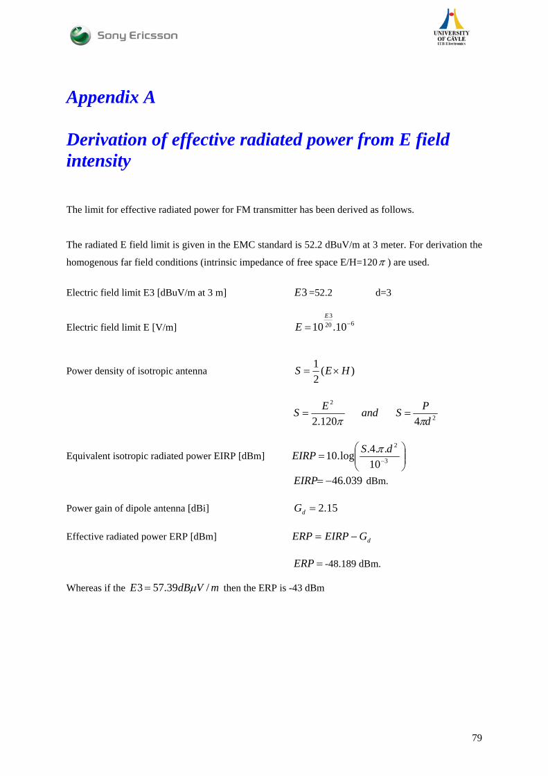
Appendix A Derivation of effective radiated power from E field intensity The limit for effective radiated power for FM transmitter has been derived as follows.

The radiated E field limit is given in the EMC standard is 52.2 dBuV/m at 3 meter. For derivation the

homogenous far field conditions (intrinsic impedance of free space E/H=120π ) are used.

Electric field limit E3 [dBuV/m at 3 m] =52.2 d=3 3E

Electric field limit E [V/m] 6203

10.10 −=E

E

Power density of isotropic antenna )(21 HES ×=

2

2

4120.2 dPSandESππ

==

Equivalent isotropic radiated power EIRP [dBm] ⎟⎟⎠

⎞⎜⎜⎝

⎛= −3

2

10..4.log.10 dSEIRP π

039.46−=EIRP dBm. Power gain of dipole antenna [dBi] 15.2=dG Effective radiated power ERP [dBm] dGEIRPERP −= =ERP -48.189 dBm. Whereas if the mVdBE /39.573 μ= then the ERP is -43 dBm

79

80

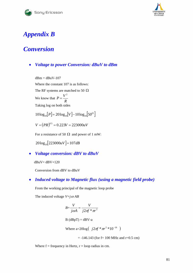
Appendix B Conversion

• Voltage to power Conversion: dBuV to dBm

dBm = dBuV-107

Where the constant 107 is as follows:

The RF systems are matched to 50 Ω

We know that R

VP2

=

Taking log on both sides

[ ] [ ] [ ]Ω−= 50log10log20log10 101010 VP

( ) uVVPRV 223000223.05.0 === For a resistance of 50 and power of 1 mW: Ω

[ ] dBuV 107223000log20 10 =

• Voltage conversion: dBV to dBuV dBuV= dBV+120 Conversion from dBV to dBuV

• Induced voltage to Magnetic flux (using a magnetic field probe)

From the working principal of the magnetic loop probe The induced voltage V=jω AB

B= 2*2 rfjV

AjV

ππω=

B (dBpT) = dBV-a Where a=20log ( )162 10**2 −rfj ππ = -146.143 (for f= 100 MHz and r=0.5 cm) Where f = frequency in Hertz, r = loop radius in cm.

81

• Magnetic Flux Density to Magnetic field intensity

dBpT=dBuA/m + 2.0 Where the constant 2.0 is as follows: The magnetic flux density B is in Teslas (T) The permeability of the medium is in Henrys per meter (H/m)

The permeability in free space is mH /10*4 70

−= πμ

By converting from T to pT and from A/m to uA/m and taking the log 240-120+20log [ ]7

10 10*4log −π =2.0

• Magnetic field to electric field dBuA/m = dBuV/m-51.5 Where the constant 51.5 is a conversion of the characteristic impedance of the free space

(120π ) into decibels:

20log [ ]π12010 =51.5

82

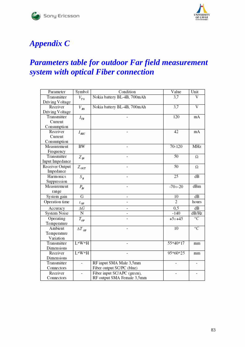
Appendix C Parameters table for outdoor Far field measurement system with optical Fiber connection

83

84

Appendix D Technical Data for the Tunable Dipole Antenna for 1 meter measurement

85

86

Appendix E

Relation between field strength and volume of FM transmitter antenna

The previous sections of this paper were about the measurement systems, result, and comparison of

the FM transmitter’s parameters between the near field and far field measurement. It is mentioned

before that the goal of the thesis is not only to propose a measurement system but also to provide a

relation between the internal loop FM antenna size and placement, input power as well as the field

strength in mobile phone FM transmitter application. The relation is based on CST software

simulation. The results can be used as a guideline for this kind antenna design, but the absolute value

of the simulation is not accurate enough. They could be used as relative relations.

E.1 Antenna structures: To see the influence of the antenna size and the placement of input power over the radiated field

strength, three models (loop antenna) are simulated at three different frequencies within FM broadcast

band which are as follows.

Figure E.1: Three different models for FM transmitter. (a) Loop length (84 mm) is folded with 5 steps (model 1). (b) Loop length (84 mm) is folded with 3 steps (model 2).

(c) Loop length (260 mm) is folded with 7 steps (model 3)

87

Except the antenna length other parameter are same for the 3 models which is tabulated in table E.1.

The 3 different frequencies are 77 MHz, 98 MHz and 108 MHz. All the radiated intensity is taken at a

distance of 3 meter (ETSI requirement) from the antenna surface.

Antenna elements Length (mm) Width (mm) Thickness(mm) Material

Chassis 100 40 2 PEC

Loop antenna (model 1) 84 2 0.2 PEC

Loop antenna (model 2) 84 2 0.2 PEC

Loop antenna (model 3) 260 2 0.2 PEC

Table E.1: antenna parameters of 3 models

E.2 Results by simulations:

(a) Frequency 77 MHz (b) frequency 77 MHz

Figure E.2 E field intensity vs. antenna length at 77 MHz. (a)using the ful antenna lenght of the three

models (b)using the antenna lenght up to 84 mm for 3 simulated models

88

(a) Frequency 95 MHz (b) frequency 95 MHz

Figure E.3 E field intensity vs. antenna length at 95 MHz .(a) Using the ful antenna lenght of the

three models (b)using the antenna lenght up to 84 mm for 3 simulated models

(a) Frequency 108 MHz (b) frequency 108 MHz

Figure E.4 E field intensity vs. antenna length at 108 MHz. (a) Using the ful antenna lenght of the

three models (b) Using the antenna lenght up to 84 mm for 3 simulated models

All results are based on 6 dBm input power which is applicable for typical mobile phone applications.

Figure E.2 (a) and (b) is for 77 MHz. Figure E.2 (b) is for large version of figure E.2(a) up to the

antenna length 84 mm and from figure E.2(b) it is shown that the E field intensity of model 2 (red

line) is higher when the antenna length is 84 mm for the three models. So it is understandable that the

placement of antenna has an influence on the radiated field intensity.

Figure E.1(b) which shows the loop placement of model 2 which is along with the edge of the PCB

length. From the same figure it is seen that when the antenna length is around 25 mm the three models

89

give almost same results (40-41 dBuV/m). So to get such a limit of field intensity at 3 meter any of the

models can be chosen. For getting a little higher field intensity (45-50 dBuV/m) may be model 2 will

be a batter choice. As it is seen from the same figure using the same antenna length, model 2 has

comparatively higher intensity.

At 95 and 108 MHz the same result is repeated like 77 MHz with increasing the value of the intensity

which is shown in figure E.3 and E.4. If we want very low radiated field then these figure shows that

we don’t need long antenna. By making the proper placement of the antenna loop it can be easily

establish proper model for FM transmitter for mobile phone applications.

Let’s see the influence of the PCB length over the radiated power. To see the influence of the PCB

length we simulated the model 1 at different frequency within the FM broadcast frequency. The

following figure shows the corresponding results.

Figure E.5 E field intensity vs. PCB length of model 1 at 3 different frequencies.

From the above figure it is shown that using a fixed antenna length here it is 84 mm (model 1), if we

change the PCB length then the radiated field intensity is decreasing with increase of PCB length. We

varied the PCB size from 80 mm to 140 mm. For other two models same explanation may be

established. But the influence of the PCB length is not too much over the E field intensity. From

figure E.5 it is shown that the deviation between the E field intensity is only 0.5 dB over the full range

of PCB length variation.

90

91

From the above discussions it may be concluded that the placement of antenna and the size of loop

have a defensible influence over the field intensity whereas the PCB length variation has less concern.

From the figures E.2, E.3 and E.4 it makes a sense that model 2 will be better for getting higher

intensity than other two models. If we want to have less intensity any of the models can be reasonable

but in model 2 the placement of the loop is simpler and occupied less space than others. So this model

will be proper enough for both requirements.