NCHRP 08-89: Applying GPS Data

to Understand Travel Behavior

ITM 2014, Baltimore MD

Research Team

• Westat | GeoStats Services

— Jean Wolf, PhD

— William Bachman, PhD

— Marcelo Simas Oliveira, PhD

• University of Illinois, Chicago

— Joshua Auld, PhD

— Kouros Mohammadian, PhD

• Parsons Brinckerhoff

— Peter Vovsha, PhD

2

Overview and Objectives

• Document use of GPS technology in the context of travel

behavior data collection

• Identify existing standard practices and guidelines

• Evaluate data processing methods and make recommendations

• This presentation will focus on the methods evaluated in Task 3

• Experiments A and B

Project Tasks

• Task 1: Conduct Background Research

• Task 2: Prepare Interim Report

• Task 3: Develop and Test Methods, Prepare Tech Memo

• Task 4: Prepare Guidelines

—Volume II

• Task 5: Prepare Final Report

—Volume I

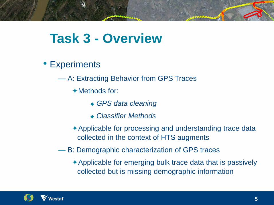
Task 3 - Overview

• Experiments

— A: Extracting Behavior from GPS Traces

Methods for:

GPS data cleaning

Classifier Methods

Applicable for processing and understanding trace data

collected in the context of HTS augments

— B: Demographic characterization of GPS traces

Applicable for emerging bulk trace data that is passively

collected but is missing demographic information

5

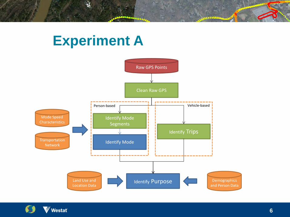
Experiment A

6

Clean Raw GPS

Identify Mode Segments

Identify Trips

Identify Mode

Identify Purpose

Raw GPS Points

Person-based Vehicle-based

Transportation Network

Land Use and Location Data

Mode Speed Characteristics

Demographics and Person Data

Experiment B

7

Data Sources

• ARC GPS person-Based HTS

— Raw GPS points

— Mode segments

— Linked Trips

• OHAS Portland smartphone data (PaceLogger)

— GPS trips reviewed by analysts

— Survey households and person data

• Later complemented by CMAP HTS

— Multi-day household sub-sample

8

A: GPS Data Cleaning

• GPS Data Cleaning

• Trip Identification

• Mode Transition

9

A: Data Cleaning

• Methods evaluated

— Stopher: Remove zero-speed points and points which

show movements of less than 15 meters.

— Lawson: Remove points based on HDOP, number of

satellites, zero speed or heading, and presence of “jumps”.

— Schuessler & Axhausen: Points are removed if their

altitude is not within the study area. They are then

smoothed and filtered by speed and acceleration.

• Findings

— Collect of HDOP, NBSAT, and instantaneous speed

— If quality indicators are not available S & A is a good

alternative

10

A: Trip Identification

• Methods evaluated

— Wolf et al.: 120 second gap between points representing

movement.

— Schuessler & Axhausen: uses clustering and dwell time.

Even though there were several rules applied to the data,

the bulk of the detection typically occurred as part of the

first point density rule.

• Findings

— Start with a simple approach to get a good first cut

— Review and validation of automated results is

recommended

12

A: Mode Transition

• Methods evaluated

— Tsui & Shalaby: Defines key transition points and then

applies heuristics to build mode segments.

— Oliveira et al.: combines dwell time, mode transitions and

cleaning (based on trip characteristics).

• Findings

— T & S performed best, identified short walk segments more

reliably

— Both methods require manual review of results

14

A: Travel Mode Identification

• Methods evaluated

— Stopher: heuristics based on point speed and GIS data.

— Oliveira: probabilistic using MNL on point speed

aggregates.

— T & S/S & A: artificial intelligence using Fuzzy Logic.

— Gonzalez: neural network.

• Findings

— Neural network performed the best, if a training dataset is

available it should be used

16

A: Trip Purpose

• Methods evaluated

— Vovsha: using MNL modeling – complex model which was

difficult to code and took considerable effort to converge.

— G & H: decision trees same set of variables – quicker to

get results and simpler to grasp.

• Findings

— Both methods performed well, but decision trees were

quicker to get results

— Recruit survey is important (person category and habitual

locations

— Simplify purpose categories is needed

— Mandatory purposes could be predicted well

18

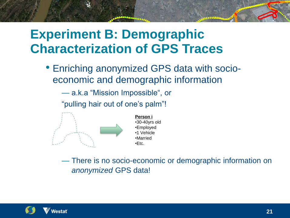
Experiment B: Demographic Characterization of GPS Traces

• Enriching anonymized GPS data with socio-economic and demographic information

— a.k.a “Mission Impossible“, or

“pulling hair out of one’s palm”!

— There is no socio-economic or demographic information on

anonymized GPS data!

21

Person i

•30-40yrs old

•Employed

•1 Vehicle

•Married

•Etc.

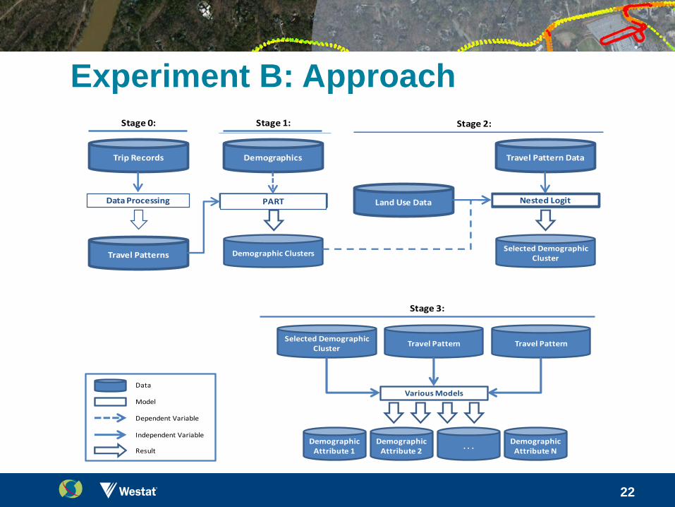
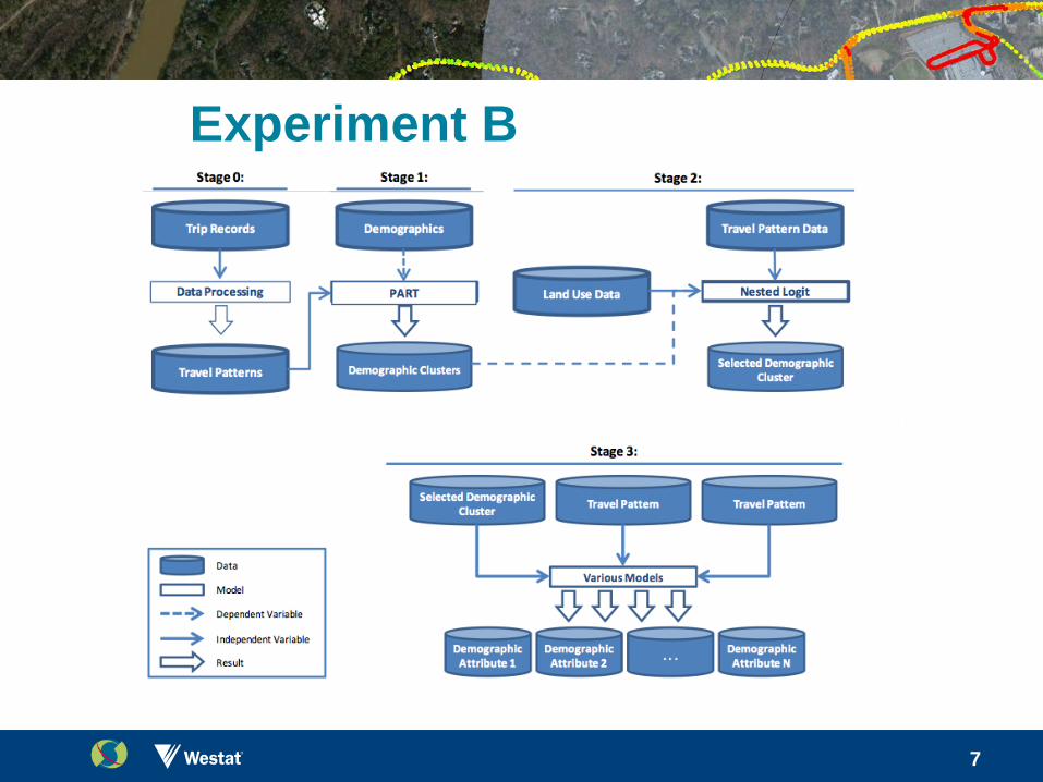
Experiment B: Approach

22

Travel Pattern Data

Travel Principal Components

PCA

Demographics

PART

Travel Pattern Clusters

K-means

Demographic Clusters

Stage 1:

Travel Pattern Data Demographics

C4.5 / PART

Selected Demographic Cluster

Stage 2:

Land Use Data

Selected Demographic Cluster

Travel Pattern

Various Models

Stage 3:

v

Travel Pattern

Demographic Attribute 1

Demographic Attribute 2

. . .Demographic Attribute N

c vv

Data

Model

Dependent Variable

Independent Variable

Result

Nested Logit

Stage 1:

Trip Records

Stage 0:

Data Processing

Travel Patterns

PART DemographicsLand Use Data

Demographics Travel Pattern Data

Data Processing

• Input general trip record format

• Process to convert to person travel characteristics

• Assumptions:

— Trips represent full day of data collection

— Trips can be uniquely linked

— Home, work and school locations can be identified

23

Input data for modeling

• One-day data is not enough… need multi-day GPS data

• Chicago Travel Tracker survey selected for model estimation

— Reformatted to match general trip input format

i.e. only person/trip id, mode, location type and activity/trip duration retained

Along with person-type info, used as dependent variables

— Similar to Portland survey, except for 2 day period

Important for addressing day-to-day variability

Can be as significant as inter-personal variability (Pas and Sundar 1995)

— Substantial sample size of over 23,000 respondents

Input data limited to approx 9700 respondents who completed two days

• Tested various modeling approaches (ANN, Decision Trees, discrete choice)

24

Experiment B: Key Findings • Multi-day data collection preferable to single day

— helps to average out intrapersonal day to day variation

• Reasonable estimates of workplace and school locations, are necessary — More detailed location databases

— longer term observation which can identify recurrent travel patterns.

• Ensuring all household members tracked and linked would help greatly — the joint trip-making travel characteristics tended to be significant in early versions of the model

• Causality between travel patterns and personal characteristics is reversed — Appears to be much weaker in going from travel pattern -> demographics

• Some person types are indistinguishable based only on travel patterns — e.g. a young child / caretaker or retiree vs. unemployed

— This is especially true for short term data collection i.e. part-time vs. full time workers

• Joint modeling of attributes is “very” difficult but important — Improves model fit

— Maintains consistency between demographic variables

25

Implementation of Tests

• Maximize reach by using Free and Open-Source Software (FOSS) tools

— R 3.0 (R Core Team, 2013) for heuristics methods and for

calling Fuzzy Logic routines in Java

— Biogeme 2.2 and Biosim (Bierlaire, 2003) for multinomial

logit choice modeling

— Weka 3 data mining tool set (Hall, et al., 2009) for neural

networks, classifier trees and clustering

— A little bit of C++ and SQL

• Code and simple instructions will be made available via NCHRP

32

Thank You!

• Final report was submitted to NCHRP in February 2014

— Stay tuned for online release

— Webinar is being scheduled

33