NBER WORKING PAPER SERIES

TRADE DISRUPTIONS AND AMERICA’S EARLY INDUSTRIALIZATION

Douglas A. IrwinJoseph H. Davis

Working Paper 9944http://www.nber.org/papers/w9944

NATIONAL BUREAU OF ECONOMIC RESEARCH1050 Massachusetts Avenue

Cambridge, MA 02138August 2003

We thank participants at the NBER Summer Institute 2003 and the Dartmouth international lunch for veryhelpful comments. Irwin thanks the National Science Foundation for financial support. The views expressedherein are those of the authors and not necessarily those of the National Bureau of Economic Research.

©2003 by Douglas A. Irwin and Joseph H. Davis. All rights reserved. Short sections of text, not to exceedtwo paragraphs, may be quoted without explicit permission provided that full credit, including © notice, isgiven to the source.

Trade Disruptions and America’s Early IndustrializationDouglas A. Irwin and Joseph H. DavisNBER Working Paper No. 9944August 2003JEL No. F1, N7

ABSTRACT

Between 1807 and 1815, U.S. imports of manufactured goods were severely cut by

Jefferson's trade embargo, subsequent non-importation measures, and the War of 1812. These

disruptions are commonly believed to have spurred early U.S. industrialization by promoting the

growth of nascent domestic manufacturers. This paper uses a newly available series on U.S.

industrial production to investigate how this protection from foreign competition affected domestic

manufacturing. On balance, the trade disruptions did not decisively accelerate U.S. industrialization

as trend growth in industrial production was little changed over this period. However, the disruptions

may have played a limited role in shifting resources from trade-dependent industries (such as

shipbuilding) to domestic infant industries (such as cotton textiles).

Douglas A. IrwinDepartment of EconomicsDartmouth CollegeHanover, NH 03755and NBERdouglas.irwin@dartmouth.edu

Joseph H. DavisThe Vanguard Groupjoseph_davis@vanguard.com

1 For example, Taussig (1931, pp. 16-17) observed that a “series of restrictive measuresblocked the accustomed channels of exchange and production, and gave an enormous stimulus tothose branches of industry whose products had before been imported. Establishments for themanufacture of cotton goods, woollen cloths, iron, glass, pottery, and other articles, sprang upwith a mushroom growth. . . . It is sufficient here to note that the restrictive legislation of 1808-

Trade Disruptions and America’s Early Industrialization

1. Introduction

Between 1807 and 1815, U.S. foreign trade was severely disrupted by Jefferson’s trade

embargo, subsequent non-importation measures, and the British blockade during the War of

1812. These disruptions prevented foreign manufactured goods from reaching the U.S. market,

thereby protecting nascent domestic industries from import competition. As a result, new

manufacturing firms were established and existing domestic producers rapidly expanded output

to replace previously imported goods. When normal commerce resumed in 1815, however, a

flood of imported manufactured goods (mainly from Britain) threatened to eliminate many of the

new producers and set back any gains to domestic manufacturers. Although it came too late to

save many of the recent domestic entrants, the tariff of 1816 helped stem the flow of imports and

stabilize the situation.

This version of events is widely accepted; economic historians have no reason to doubt

that, by keeping British manufactured goods out of the U.S. market, the trade disruptions helped

stimulate domestic production by import-competing industries. An open question, however, is

whether the seven-year trade disruption decisively accelerated America’s industrialization,

despite the setback in 1815, or merely provided a temporary and short-lived boost to some

domestic manufacturers. Limited data on early U.S. industries have prevented any clear cut

answer from emerging. Older works document to the blossoming of manufacturing around this

period, but mainly provide descriptive evidence from the period.1 More recent research has

-2-

15 was, for the time being, equivalent to extreme protection.”

2 Lebergott (1984, p. 126), Rosenbloom (2002), and others have observed the strikinginverse correlation between shipping volume and incorporations of cotton textile firms. Inaddition, Sokoloff (1988) notes a small wave of patenting activity around the time of the tradedisruptions.

provided some limited quantitative evidence by focusing on indirect measures of manufacturing

activity, such as incorporations or patents, both of which increased as well.2 But the lack of data

from the period has impeded efforts to determine precisely how the trade disruptions affected the

American economy.

This paper addresses the question of how the trade disruptions affected early U.S.

manufacturing by using a new index of industrial production by Davis (2002). The index can be

decomposed into its constituent elements, permitting a more refined look at the impact of trade

disruptions on different parts of the early manufacturing economy, such as domestic infant

industries (e.g., cotton textiles) and trade-dependent industries (e.g., shipbuilding).

This index reveals that, on balance, the trade disruptions did not decisively accelerate

U.S. industrialization; indeed, the trend growth in total industrial production is little changed

over this period. However, the trend in aggregate industrial production masks a sharp

divergence between the fate of infant industries (which boomed) and trade-dependent industries

(which suffered). The United States entered the post-War of 1812 period with nearly 20 percent

more infant industry production, and about 30 percent less trade-dependent industry production,

than otherwise would have been expected. Yet our analysis suggests that the trade shocks have

largely temporary effects on industrial production and therefore are not able to account for this

permanent shift in resource allocation. Rather, shifts in the composition of domestic and

-3-

3 Adams (1980) and Goldin and Lewis (1980) examine the impact of this booming re-export trade on the American economy.

international demand, the Tariff of 1816, and other factors may have been responsible for this

reallocation between industries.

2. Trade Disruptions and Domestic Industries

At first, U.S. foreign commerce benefitted from the war that broke out between Britain

and France in 1793. As a neutral country, American merchants quickly took advantage of the

void left by the combatants in shipping goods from North America and the Carribean to Western

Europe. U.S. re-exports boomed, growing from about $1 million in 1792 to nearly $40 million

by 1800.3 As the European hostilities intensified, however, the United States gradually became

embroiled in the conflict. The British and French navies began harassing American merchants,

confiscating their ships and cargoes, and impressing their sailors as each country sought to

strangle the economy of the other.

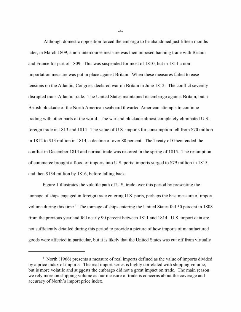
In response, President Thomas Jefferson requested that Congress enact a trade embargo

in December 1807. The embargo prevented U.S. ships from sailing to foreign destinations and

its purpose was to prevent further losses to the merchant marine while denying Britain and

France much needed supplies. Jefferson hoped that this “peaceful coercion” would convince the

two powers to change their policy and respect neutral shipping. The embargo was a sharp blow

to trade: imports for consumption fell 60 percent in 1808 from the previous year; a larger fall

was prevented because American ships in Europe at the time the embargo was announced were

allowed to return home and unload their cargoes.

-4-

4 North (1966) presents a measure of real imports defined as the value of imports dividedby a price index of imports. The real import series is highly correlated with shipping volume,but is more volatile and suggests the embargo did not a great impact on trade. The main reasonwe rely more on shipping volume as our measure of trade is concerns about the coverage andaccuracy of North’s import price index.

Although domestic opposition forced the embargo to be abandoned just fifteen months

later, in March 1809, a non-intercourse measure was then imposed banning trade with Britain

and France for part of 1809. This was suspended for most of 1810, but in 1811 a non-

importation measure was put in place against Britain. When these measures failed to ease

tensions on the Atlantic, Congress declared war on Britain in June 1812. The conflict severely

disrupted trans-Atlantic trade. The United States maintained its embargo against Britain, but a

British blockade of the North American seaboard thwarted American attempts to continue

trading with other parts of the world. The war and blockade almost completely eliminated U.S.

foreign trade in 1813 and 1814. The value of U.S. imports for consumption fell from $70 million

in 1812 to $13 million in 1814, a decline of over 80 percent. The Treaty of Ghent ended the

conflict in December 1814 and normal trade was restored in the spring of 1815. The resumption

of commerce brought a flood of imports into U.S. ports: imports surged to $79 million in 1815

and then $134 million by 1816, before falling back.

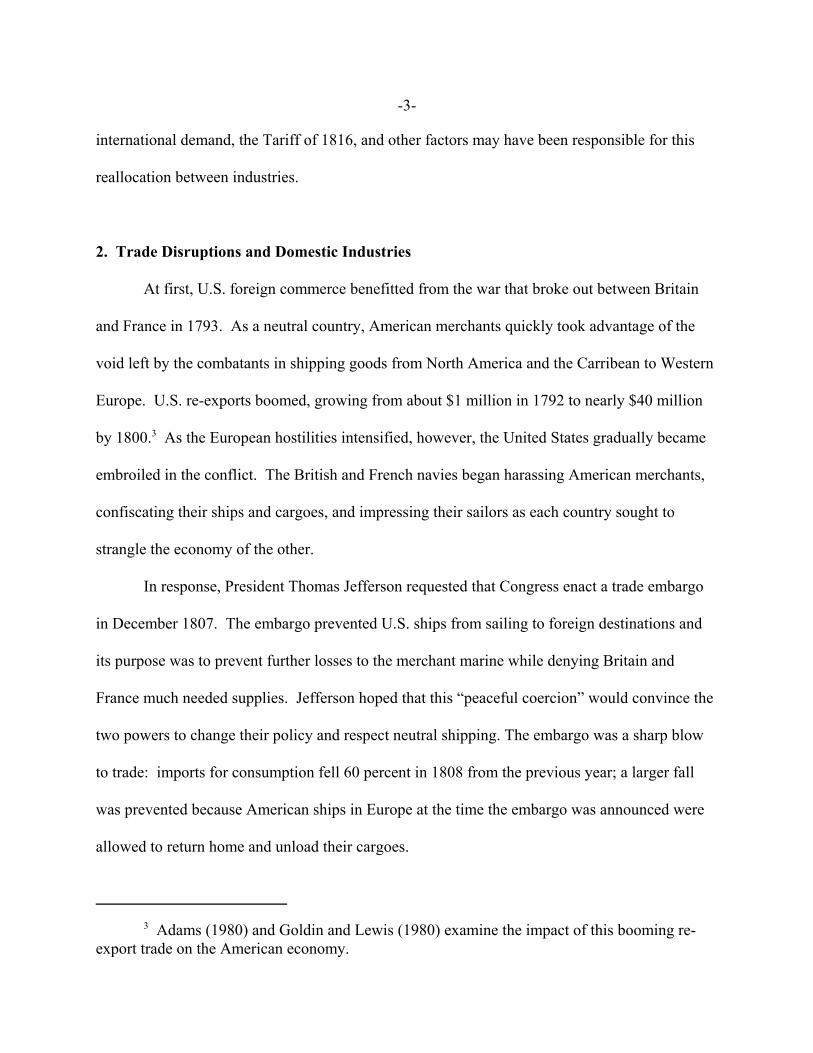
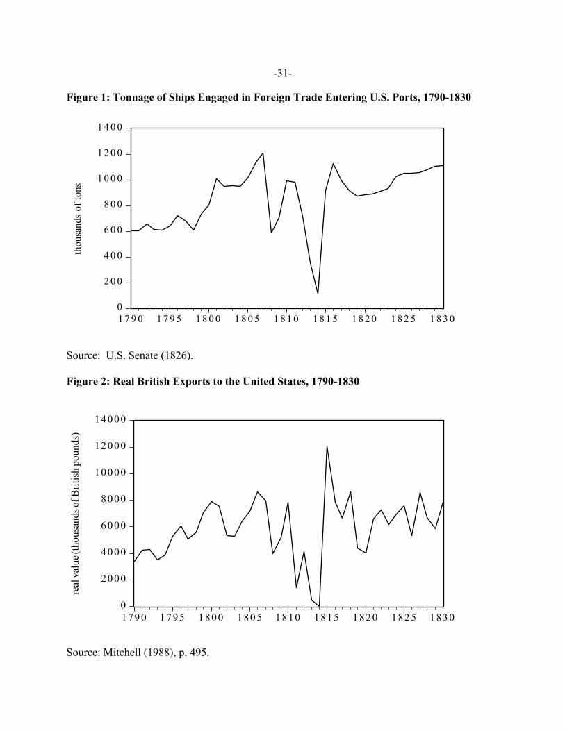
Figure 1 illustrates the volatile path of U.S. trade over this period by presenting the

tonnage of ships engaged in foreign trade entering U.S. ports, perhaps the best measure of import

volume during this time.4 The tonnage of ships entering the United States fell 50 percent in 1808

from the previous year and fell nearly 90 percent between 1811 and 1814. U.S. import data are

not sufficiently detailed during this period to provide a picture of how imports of manufactured

goods were affected in particular, but it is likely that the United States was cut off from virtually

-5-

all foreign manufactured goods. Imports of manufactured goods came overwhelming from

Britain, and the official value (real) British exports to the United States fell to extremely low

levels from 1811 until 1815, as Figure 2 illustrates. The U.S. trade that did take place during this

period was largely with countries in the Carribean rather than in Europe and thus probably did

not consist of industrial products.

As noted in the introduction, the lack of economic data from this period has hampered

efforts to determine how these severe trade disruptions affected early American industry.

However, Davis’s (2002) recently constructed index of industrial production for the 1790-1915

period provides a clearer view of the state of U.S. manufacturing during this time. This annual

index incorporates 37 physical-volume series in the pre-Civil War period to gauge

manufacturing activity in a manner similar to how the Federal Reserve Board’s index currently

measures U.S. industrial production. While Davis’s original index possesses complete coverage

from 1826 on, moderate attrition occurs further back in time. Consequently, we have

constructed a version of the original Davis index whose coverage preserves comparability of

index changes over time. Specifically, the special variant of the index includes only industries

that existed on the eve of the embargo (and whose annual direct or indirect output measures were

available before 1808) or that emerged as entirely new industries between the embargo period

and the base 1850 census year of the index. These selection criteria retained 27 of the 37

original antebellum industries in the original Davis index, representing 61.4 percent of the value-

added weight of the 1850 base year.

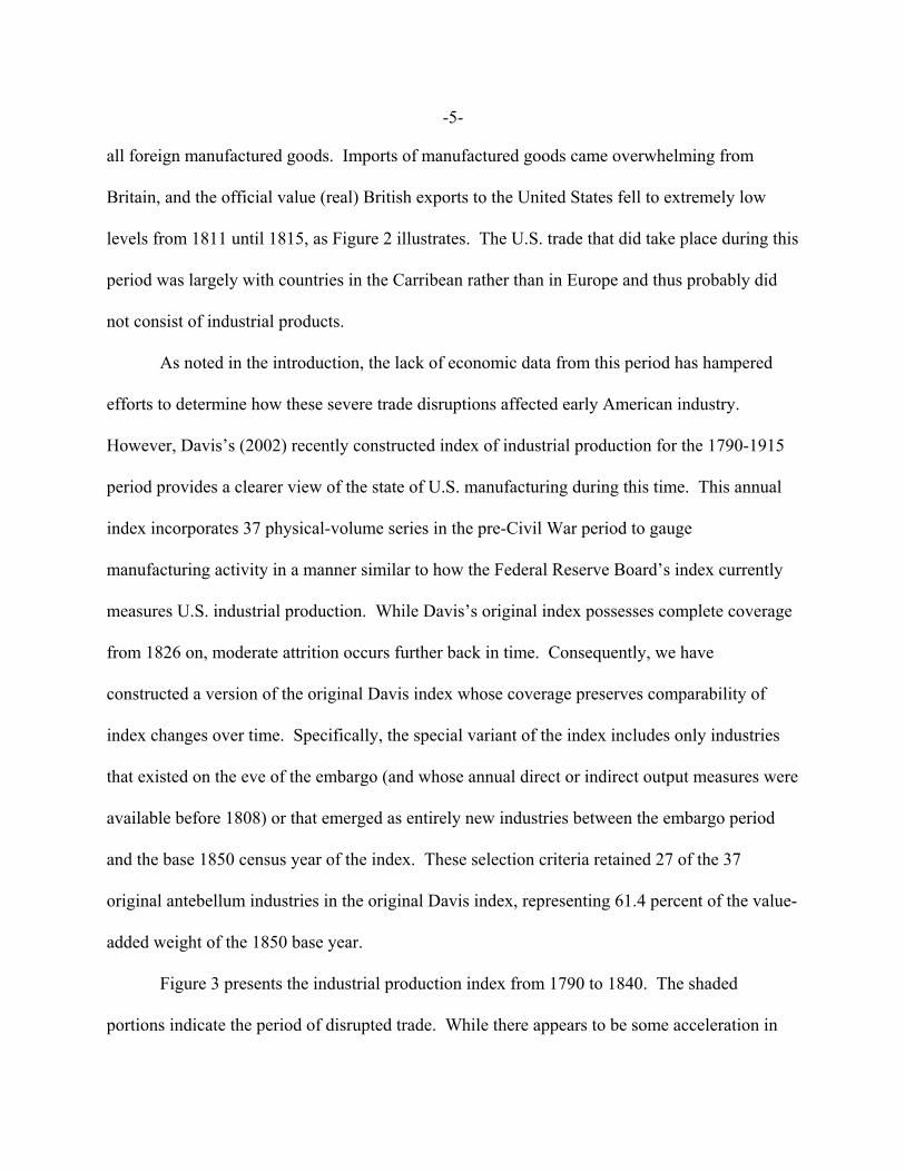
Figure 3 presents the industrial production index from 1790 to 1840. The shaded

portions indicate the period of disrupted trade. While there appears to be some acceleration in

-6-

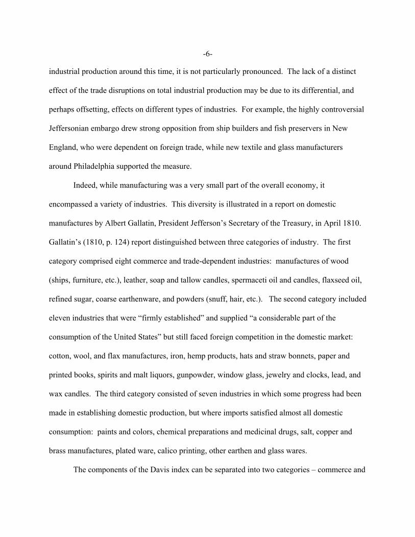
industrial production around this time, it is not particularly pronounced. The lack of a distinct

effect of the trade disruptions on total industrial production may be due to its differential, and

perhaps offsetting, effects on different types of industries. For example, the highly controversial

Jeffersonian embargo drew strong opposition from ship builders and fish preservers in New

England, who were dependent on foreign trade, while new textile and glass manufacturers

around Philadelphia supported the measure.

Indeed, while manufacturing was a very small part of the overall economy, it

encompassed a variety of industries. This diversity is illustrated in a report on domestic

manufactures by Albert Gallatin, President Jefferson’s Secretary of the Treasury, in April 1810.

Gallatin’s (1810, p. 124) report distinguished between three categories of industry. The first

category comprised eight commerce and trade-dependent industries: manufactures of wood

(ships, furniture, etc.), leather, soap and tallow candles, spermaceti oil and candles, flaxseed oil,

refined sugar, coarse earthenware, and powders (snuff, hair, etc.). The second category included

eleven industries that were “firmly established” and supplied “a considerable part of the

consumption of the United States” but still faced foreign competition in the domestic market:

cotton, wool, and flax manufactures, iron, hemp products, hats and straw bonnets, paper and

printed books, spirits and malt liquors, gunpowder, window glass, jewelry and clocks, lead, and

wax candles. The third category consisted of seven industries in which some progress had been

made in establishing domestic production, but where imports satisfied almost all domestic

consumption: paints and colors, chemical preparations and medicinal drugs, salt, copper and

brass manufactures, plated ware, calico printing, other earthen and glass wares.

The components of the Davis index can be separated into two categories – commerce and

-7-

5 In terms of 1850 value-added weights, the relative value-added weights are split ratherevenly among Gallatin’s classifications of (1) trade-dependent industries (eight series,representing 32 percent of the index’s value added), (2) “firmly established” domestic industries(14 series, 27 percent), and (3) import-competing “infant” industries (five series, 41 percent).

trade-dependent industries and domestic import-competing “infant” industries – that roughly

correspond to Gallatin’s designation. (For our analysis, Gallatin’s second and third categories

are combined because, on the eve of the embargo, few if any domestic industries were truly free

from any import competition.) The 27 quantity-based components in this early American output

index correspond closely with the 26 industries cited by Gallatin in his three categories of

industry. Commerce and trade-dependent industries include merchant shipbuilding, refined

sugar, sperm- and whale-oil refining, wheat flour milling, fish curing, whale bone and copper.

Domestic infant industries include domestic cotton consumption (a proxy for textile output),

newspaper circulation, coal production, hog packing, navy vessels, music organs, hand fire

engines, firearms, salt production, army wool stockings, cloth regalia, and army boots and shoes.

As would be expected of the early developing American economy, the values of the commerce

and trade-dependent sub-index are larger than the sub-index of the domestic infant industries

during the period under examination.5

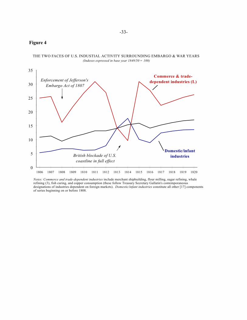
Figure 4 shows the relative importance of these two categories and, more importantly, the

markedly different effect of the trade disruptions on them. Trade-dependent industries were

adversely affected by both the embargo and the wartime blockade, but much more severely by

the latter. These trade-dependent industries experienced a drop in production of nearly 70

percent between 1811 and 1814. However, production quickly rebounded after the war. Among

the domestic infant industries, there does not appear to have been much import substitution

-8-

6 For example, Rosenbloom (2002) argues that the expansion of U.S. textile productionin the early nineteenth century is best understood as a path-dependent process initiated by theprotection provided by the trade disruptions of this period.

during the 1807-1809 embargo, but a substantial amount during the war. Infant industry

production nearly tripled between 1811 and 1814, but fell back once normal commerce resumed.

This separation reveals why total industrial production shows little sign of acceleration

during this period. Any gains to domestic infant industries were largely offset by losses to trade-

dependent industries, thus muting any pronounced impact on manufacturing overall. The trade

shocks of the 1812 to 1814 period clearly had important, temporary effects on the distribution of

industrial production across these differently situated categories, but did it have more permanent

effects as well? Did the trade disruptions decisively accelerate production by import-competing

industries or just boost their fortunes temporarily? And was the damage done to trade-dependent

industries persistent or transitory as well?

3. The Effect of Import Shocks on Industrial Production

The main question that we seek to answer is whether the trade disruption had temporary

or permanent effects on the component levels of industrial production. If trade shocks had

transitory effects on production, then temporary protection from imports would boost the level of

industrial production in the short-term, but it would then revert back to the level dictated by its

trend growth. If trade shocks had permanent effects on production, then temporary protection

from imports would lead to a persistently higher level of output.6

This section considers three different methods for examining different aspects of this

-9-

question: unit root tests, linear trend regressions, and estimates of the reduced-form relationship

between trade shocks and production.

A. Unit Root Tests

As a first pass at this question, we can test for a unit root (stochastic trend) in the

industrial production indices. The unit root test helps indicate whether any random shock to

production, without reference to trade shocks in particular, has permanent or temporary effects

on the level of production. If the test fails to reject the hypothesis of a unit root, then the shocks

to output are persistent and have a permanent effect on the level of production. If the test rejects

the existence of a unit root, then the alternative could be that industrial production is

characterized by temporary deviations from a deterministic trend, although rejection of a specific

null hypothesis does not imply acceptance of any particular alternative.

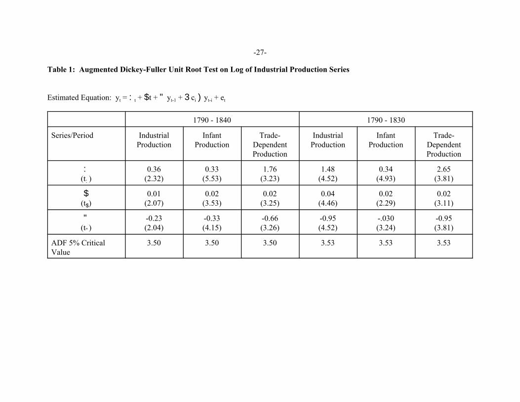
Table 1 presents augmented Dickey-Fuller (ADF) unit root tests for the three industrial

production series. The coefficient of interest is that on the lagged level of production (") and the

null hypothesis of a unit root is that " = 0. If the absolute value of the t-statistic on " exceeds

the ADF critical value, then the hypothesis of a unit root can be rejected. For total industrial

production during the sample period 1790-1840, the ADF test statistic indicates that the

hypothesis of a unit root cannot be rejected at the 5 percent level, i.e., we cannot reject the

existence of a unit root in which some fraction of an innovation is permanent. Interestingly, for

infant industry production, however, we can reject the hypothesis of a unit root. This goes

against the path dependence or hysteresis story and is surprising because these are precisely the

types of industries in which temporary protection might be thought to lead to permanent gains to

output. In the case of trade-dependent industries, the hypothesis of a unit root cannot be rejected

-10-

at the 5 percent level, but it can at the 10 percent level and the large size of the coefficient

indicates that the series exhibits substantial mean reversion.

Perron (1989) argues that the conventional ADF t-statistic frequently accepts the null

hypothesis of a unit-root when the true data-generating process is in fact trend stationary with a

break in the intercept or the slope of the trend function. Thus, structural breaks in levels or

trends in the series can bias tests against rejecting the null of a unit root. For reasons that will be

discussed later, there may be a structural shift in the trend growth of overall industrial production

in the early 1830s. Therefore, the second part of Table 1 examines the ADF test statistics for the

period of 1790 to 1830. During this period, we can reject the hypothesis of a unit root in

industrial production and in trade-dependent production at the 5 percent confidence level. Now,

however, we cannot reject the hypothesis for infant production, although we can at the 10

percent level.

Thus, we conclude that the evidence in favor of a unit root in industrial production (i.e.,

that disturbances to production are permanent) is relatively weak but still uncertain.

B. Linear Trend Forecast

If innovations to production are not substantially permanent, then an alternative

specification is to consider industrial production as stationary fluctuations around a deterministic

trend with a stationary autoregressive component, such as:

(1) log yt = : + $ t + " log yt-1 + (1 DISRUPTION + (2 POSTWAR + et

where yt is industrial production, : is a constant, t is a time trend, and et is a random error term.

This specification includes two dummy variables that allow for shifts in the level of production

during the embargo and blockade years (DISRUPTION, taking the value of one in 1808 and

-11-

7 Data from the 1790s is not used in this regression because the trend rate of growth wasmuch higher during that decade; the coefficient on time from 1790 to 1807 is 0.12 with astandard error of 0.01.

from 1812-1814) and during the post-war period (POSTWAR, which takes the value of one for

the period from 1817 to 1840).

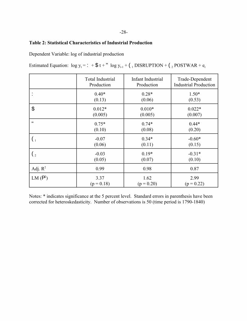
Table 2 presents the results from estimating this equation using the three industrial

production series from 1791 to 1840. For total industrial production, in the first column, the

coefficients on the dummy variables for the trade disruption and the post-war periods are small

and not statistically significant. This indicates that the disruptions had little impact on the level

of overall industrial production. However, the results are quite different for infant and trade-

dependent industries. During the trade disruption period, infant industry production was 34

percent above, while trade-dependent production was 60 percent below, what might otherwise

have been expected. After the war, the level of infant industry production was nearly 20 percent

above what might have been expected prior to the war, while trade-dependent production was

more than 30 percent below what would have been expected.

This regression suggests that infant industries came out of the war with a significantly

higher level of production than might otherwise have been anticipated. A result of virtually the

same magnitude comes from asking whether infant industry production was higher in 1820 or

1825 than one would have anticipated based on a simple linear extrapolation of its trend growth

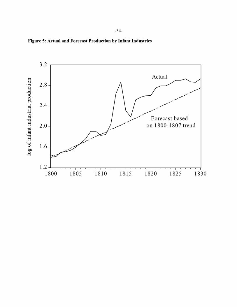
from the period prior to the trade disruption. Figure 4 illustrates this by comparing actual and

predicted infant industry production based on a simple forecast of production using only a

constant and time trend from 1800 to 1807. In this regression, the coefficient on time is 0.045,

with a standard error of 0.007, with an adjusted R2 of 0.89.7 In 1820, actual infant industry

-12-

8 We also tested for, but found no evidence of, a change in trend growth during thoseperiods, i.e., it appears that the level of production was affected but not its growth rate. Inaddition, other variables, such as the average tariff rate or annual estimates of gross domesticproduct (a potential demand-shift variable), are not statistically significant and do not greatlyaffect these estimates.

production is 13 percent above the forecast production. For the period 1820 to 1825, on average,

the actual is 15 percent above the simple forecast. In 1816, actual production is almost the same

as predicted production, but imports were abnormally high in both 1815 and 1816 as trade was

adjusting to the end of the war.

This evidence suggests that the United States emerged from the War of 1812 with a

different allocation of resources between these two industrial sectors, but not more industrial

production overall.8 The next question is whether the change in industry composition can be

linked to the trade disruptions themselves.

C. Effect of Trade Shocks

To examine the impact of trade disruptions on industrial production directly, we turn to

some reduced-form estimates of the relationship between the two. In many ways, the question of

how import shocks affect industrial production is analogous to how oil price shocks affect GDP,

the subject of a much recent research. As described in Hamilton (2003), this analysis usually

starts with a simple autoregressive distributed lag specification such as:

(2) ) log yt = : + " ) log yt-1 + $0 ) log (TONt)+ $1 ) log (TONt-1) + $2 ) log (TONt-2) +

,t,

where y is industrial production, TON is the tonnage of ships engaged in foreign trade entering

U.S. ports, and , is a random error term. The coefficient $0 captures the contemporaneous effect

of the trade shock on industrial production. By recursive substitution, the effect of a change in

-13-

tonnage at time t-1 on industrial production at time t can be represented as "$0 + $1, the effect of

a change in tonnage at time t-2 on industrial production at time t can be represented as "2$0 +

"$1 + $2, the effect of a change in tonnage at time t-3 on industrial production at time t can be

represented as "3$0 + "2$1 + "$2, etc. The sum of these effects gives us the total impact of a

change in tonnage on industrial production.

Equation 2 is frequently estimated by ordinary least squares. However, a potential

concern is that changes in industrial production and tonnage could be driven by a common

factor, such as demand shocks. For example, an increase in domestic demand for manufactured

goods could lead to an increase in imports and an increase in domestic production. Therefore,

following Hamilton (2003), we attempt to isolate the component of the change in trade that can

be attributed strictly to exogenous, non-demand factors – namely, the embargo and war – by

creating a quantitative dummy variable for the change in the log of shipping tonnage for the

years 1808 and 1812 to 1815. This quantitative dummy variable is not a zero-one variable, but

one that takes the actual value of the change in those specific years and is zero otherwise.

Because these shocks (all negative, except for 1815) are being driven strictly by American or

British policy decisions, all are likely to be exogenous to other factors driving industrial

production, such as demand or supply shocks. This quantitative dummy variable and its lags are

used as instruments in an instrumental variables estimation of equation (2).

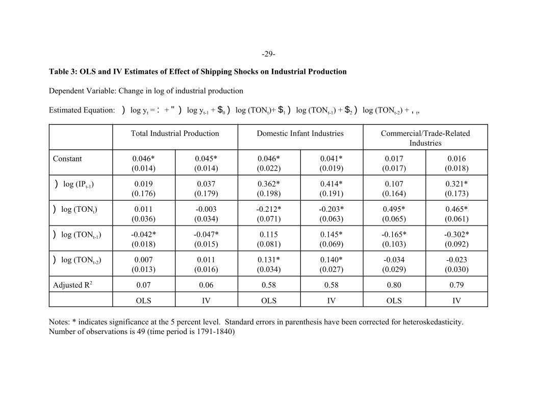
Table 3 presents the OLS and IV estimates of equation (2) for the effect of changes in

shipping tonnage on total industrial production, domestic infant industry production, and trade-

dependent production. The first two columns relating to total industrial production show that the

coefficient on contemporaneous tonnage is not associated with any significant change in

-14-

industrial production. The coefficient on lagged tonnage suggests that a ten percent reduction in

shipping volume results in a 0.42 percent increase (OLS estimate) or a 0.47 percent increase (IV

estimate) in industrial production in the next year. This implies a relatively modest effect, but

obviously a larger and more prolonged disruption to imports would have a substantial impact on

industrial output. The difference between the OLS and IV results is not substantial, suggesting

that identification in the OLS case is really being driven by the few but large shocks around 1808

to 1815. The coefficient on the second lag on tonnage is very small and statistically

insignificant.

The results are strikingly different for infant and trade-dependent industries. In contrast

to the total industrial production regressions, the explanatory power of the regressions for these

industries is very high, particularly for a first-difference regression. In the IV case for infant

industries, the coefficient on contemporaneous tonnage indicates that a 10 percent decrease in

tonnage increases production by 2.0 percent. However, the coefficients on the one and two year

lags on tonnage carry the opposite sign of the impact coefficient and are sizeable enough to more

than offset the initial impact of the shock. One year after a 10 percent negative tonnage shock,

infant industry production is just 1.4 percent higher and two years after the shock it is essentially

back to where it started.

In contrast, for trade-dependent industries, a 10 percent reduction in tonnage reduces

output in these industries immediately by about 4.7 percent (IV coefficient). The coefficients on

the lags are again the opposite sign of the impact coefficient, but the magnitude is less and the

second lag is small and insignificant. The implication here is that, one year after a 10 percent

negative tonnage shock, production by trade-dependent industries is 3.2 percent lower and two

-15-

years after production is 2.4 percent lower.

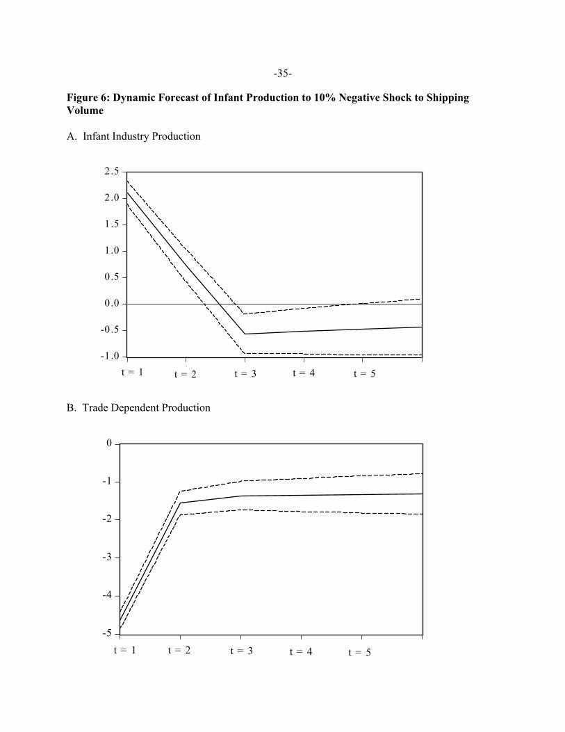
Figure 6 depicts the dynamic forecasts of infant and trade-dependent production from a

10 percent negative tonnage shock at time t = 1. Due to the use of annual data and only two

lagged values on tonnage, the responses are very choppy and do not display any new information

beyond two periods after the shock (t = 3). But the figure does illustrate that, according to the

results on Table 3, shocks to trade-dependent industries appear to be more persistent than in the

case of infant industries.

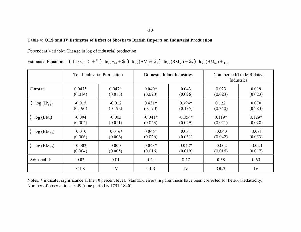
As a check on these results, Table 4 presents estimates using the change in the log of real

imports from Britain (i.e., the official value of British exports to the United States) instead of

shipping tonnage. The British variable could be a better measure of imports of manufactured

goods than overall tonnage because Britain was the source of most of those goods. The results

are quite similar to those using tonnage, particularly with respect to the mean-reverting behavior

of infant industry production to trade shocks. In results we do not report, we also used real

imports from North (1966), which also yielded econometric findings similar to those in Table 2.

D. Interpretation

The previous subsection concluded that, from 1817, the United States had a level of

infant industry production that was about 20 percent higher than one would have anticipated

based on prewar trends. In addition, the level of trade-dependent industry production was about

30 percent lower than one would have anticipated. Although this description of the data was not

directly tied to the trade disruption itself, it is very tempting to make that attribution. However,

the results reported above tend to suggest that trade shocks have only temporary effects on the

level of infant production and small permanent effects on the level of trade-dependent

-16-

9 See Irwin and Temin (2001), Table 4 and Figure 5.

production.

If trade shocks themselves do not appear to be responsible for the permanent changes in

the composition of industrial production, several other factors could have intervened in the

immediate post-war period to alter the allocation of resources between infant and trade-

dependent production. The two most likely candidates are the Tariff of 1816 and the changing

composition of domestic and international demand. The Tariff of 1816 explicitly aimed to

protect domestic industries from foreign competition and may have changed the structure of

duties across goods to shift the composition of imports away from manufactured goods.

Although Figure 1 shows that the volume of imports (shipping tonnage) returned to its prewar

level by 1816, the measure of import volume here comprises all imports, not manufactured

goods. Figure 2 indicates that import from Britain fell from 1815 to 1820 and then never

reached their pre-war peak. For example, the value and volume of imports of cotton textiles

from Britain was much lower in 1816 and 1817 than it had been in 1815 or even prior to the war,

although whether this was due to the Tariff of 1816 or postwar economic difficulties is difficult

to determine).9 This might account for the path dependence that Rosenbloom (2002) argues was

present in the case of cotton textiles.

Indeed, it should be noted that the effects of a trade disruption are not comparable to the

effects of a tariff on imported manufactured goods. An import tariff could have targeted specific

types of manufactured goods without disrupting trade overall or harming trade-dependent

manufacturers in quite the way they were punished during this period. In addition, although it is

commonly believed that the import surge of 1815 could have been prevented had the Tariff of

-17-

10 In forming the tariff of 1816, Congress relied heavily on the report prepared byAlexander Dallas, the Secretary of the Treasury in the Madison administration. Like Gallatin’s1810 report, Dallas considered three classes of industry, (i) mature industries that were “firmlyand permanently established” and supplied most of domestic consumption, (ii) industries“recently or partially established” which supplied part of domestic consumption but, “withproper cultivation, are capable of being matured to the whole extent of demand,” and (iii)industries “so slightly cultivated as to leave the demand of the country wholly or almost whollydependant upon foreign sources for supply.” Examples from the first class included wood, hats,iron castings, window glass, leather, paper and printing. Examples from the second classincluded: course cotton and woolen goods, larger iron goods, and beer and spirits. Examples ofthe third class included: fine cotton goods, linens and silk goods, woollen blankets and carpets,china and earthenware, other glass products.

1816 been enacted more quickly, in fact imports in that year paid the higher wartime duties that

were still in effect (but which had affected trade with Britain very little owing to the embargo

and blockade).10

Another possible explanation for the compositional shift in industrial production is the

change in domestic and international demand after the war. For more than a decade prior to the

trade disruptions, Britain and France had been engaged in a protracted war. This war raised the

demand for U.S. ships and other exported goods to abnormally high levels. After the war, as

European demand for these products fell to normal levels, U.S. production in these trade-

dependent industries fell permanently as well. Thus the decline in trade-dependent production

was not a consequence of the trade disruptions themselves, but to a shift in foreign demand after

the war. Similarly, with respect to infant industrial production, technological changes helped

bring about a decline in household production of goods such as clothing and a shift to factory

production, thereby raising domestic production permanently. Therefore, shifts in the

composition of foreign demand and domestic household demand could plausibly account for

some of the observed reallocation between trade-dependent and infant production.

-18-

11 In April 1816, Henry Brougham stated in Parliament that “it was well worth while toincur a loss upon the first exportation, in order, by the glut, to stifle, in the cradle, those risingmanufactures in the United States, which the war had forced into existence, contrary to thenature of things” (quoted in Clark 1929, p. 240). This remark was widely noted in the UnitedStates and interpreted to mean that the import surges in 1815 and 1816 had been deliberateattempts to destroy U.S. manufacturers.

Neither the tariff nor the demand explanation is directly testable at this level of

aggregation, so we are left with some ambiguity about the precise impact of the trade disruptions

on the allocation of resources across manufacturing industries. We know that infant industry

production was much higher after the war, and trade-dependent production was much lower after

the war, but our results do not suggest that this is attributable solely to the trade shocks that

confronted producers.11

However, a stronger conclusion is that the trade disruptions did not accelerate U.S.

industrialization overall. Evidence consistent with this conclusion is that total U.S. industrial

production relative to that of Britain (using the Crafts and Harley 1992 index) does not show a

pronounced acceleration during the 1810s or 1820s. Rather, as Davis (2002) reports, U.S.

industrial output surges in the early 1830s and again in the mid 1840s relative to that in Britain.

4. What Differentiated Successful and Unsuccessful Industries?

The quantitative evidence presented above can be supplemented with qualitative

evidence on specific industries. This qualitative evidence is suggestive about some of the factors

that differentiated industries that grew during the trade disruption and continued to flourish after

the war from those that grew during the disruption but floundered in the postwar period, and

from those that failed to grow at all.

-19-

12 According to Ware (1926, pp. 43-44), the short lived Jeffersonian embargo did nothelp the New England cotton textile industry much: “the increase of mill building during theseyears has led to the conclusion that the artificial stimulus of the embargo was responsible for thesuccessful establishment of the cotton industry, but in the light of the fact that mills were forcedby the destruction of their markets to curtail their expansion, dismiss some of their help, andstruggle to dispose of the goods left on their hands, this conclusion ceases to be convincing.”

The industries that benefitted from the trade disruption tended to have low barriers to

entry. In the U.S. context, these were industries that were not capital-intensive or have

demanding technology requirements. In many instances, low barriers to entry also meant low

barriers to exit, and thus some other element – such as the acquisition of technology or the

accumulation or importation of human capital – was required to ensure the industry “stuck” in

the United States after the flow of imported manufactures resumed.

The cotton textile industry is one that many have believed benefitted permanently from

the stimulus of the trade disruption (see, for example, Rosenbloom 2002). The trade disruptions

triggered large scale entry into the industry, particularly in New England. According to

Gallatin’s 1810 Report on Manufactures, the number of operational spinning mills grew from 15

before 1808 to 62 in 1809, with many more under construction.12 The construction costs and

technological requirements for setting up spinning mills was relatively low. But the most

important change in the cotton textile industry around the trade disruptions, however, was the

shift from simple spinning of yarn to mechanical weaving, particularly with the introduction of

the power loom by the Boston Manufacturing Company, established in 1813 by Francis Lowell

at Waltham, Massachusetts. By 1815, this technology produced cloth at half the price of hand

woven cloth (Jeremy 1981, p. 101).

The adoption of the power loom ensured that many of the new entrants would be able to

-20-

13 Jeremy (1981, p. 151) observes that, from 1809 to 1813, the rate of immigration byBritish textile machine-making workers increased from previous years, but notes that “the extentof the increase in the immigration of industrial workers between 1809-1813 and the 1820s maybe magnified and distorted by . . . [the] disturbed Anglo-American relations prior to the War of1812 [which] reduced earlier levels of immigration.”

survive the postwar trade competition. The question is whether the shift to power looms can be

linked to the trade disruptions, or would the adoption of this technology have occurred in the

absence of the disruptions anyway? According to Jeremy (1981, p. 93), “In 1812 the British

were on the way to solving many of the technical problems of power weaving,” which suggests

that the United States adopted this technology as soon as it was ripe and ready. Although the

profitability of power loom adoption was high due to the trade disruptions, the United States had

previously acquired other British textile technologies relatively quickly during earlier period of

normal trade. Thus, it is not evident that the trade disruptions were decisive. An indirect way in

which the disruptions could have facilitated technology transfer is through the immigration of

skilled workers from Britain, but the evidence on this is not conclusive.13 (Even if the trade

disruptions had not occurred, there was also ample room for an expansion of U.S.-based factory

production at the expense of home production of clothing.)

A comparison of the New England and Philadelphia cotton textile industries suggests that

the power loom was quite important to the survival of the industry. The New England industry

adopted the power loom and easily survived into the post-war era, while the industry around

Philadelphia boomed with the trade disruption but, lacking significant investment in power

looms, withered once normal commerce resumed. The 1810 Census records that 206 looms were

in operation in Philadelphia, but only 140 – of which just 65 were in operation – in 1820

-21-

14 Textile employment fell from 3,500 in 1816 to just 400 in 1819 and just 200 in theCensus of 1820. As a result, “Philadelphia millmen, by 1820, looked back on the midteens as aset of golden years,” according to Scranton (1987, p. 76).

(Scranton 1987, p. 88).14

If technological adoption was an important factor in textiles, other industries failed

because the requisite technology had not arrived on American shores. Pocket watches were very

complicated products that were imported almost exclusively from Europe before the 1850s.

Most advertised American “watchmakers” were in fact watch repairers or jewelry-makers.

However, the embargo of 1807 encouraged Luther Goddard in Massachusetts to attempt to

manufacture watches domestically in his repair shop. According to Bailey (1975, 190-5),

Goddard made fewer than 500 watches between 1809 and 1817. The first watches made were of

poor quality and took considerable time to build; he proved unable to compete effectively with

European craftsmanship. Several decades passed before domestic production was firmly

established.

In the case of medicines, low barriers to entry combined with domestic human capital to

ensure the continuing success of the industry after trade resumed. The production of medicines

required relatively little physical capital and was often a side business of physicians. Liebenau

(1987, p. 11) notes that the foundation for the U.S. pharmaceutical industry was “laid between

1818 and 1822 with the establishment of several chemical manufacturers.” America had been

formerly dependent on British imports for medicine, but “with the economic disorder created by

the war of 1812 and its aftermath, this pattern of dependence was broken.” Liebenau observes

that the manufacture of most common medicines was within reach for most apothecaries, as

there was little need for capital investment and only a general knowledge of pharmacy required

-22-

to produce basic remedies such as quinine sulphate, opium powders, and calomel. Production of

these medicines were not capital intensive, but rather human-capital intensive. And Philadelphia

had large concentration of well-educated German immigrant physicians and chemists, which

contributed to the advances made by the industry at this time.

The glass industry – mainly engaged in the production of window glass – may also be

one in which there were low entry barriers, but there was no special human capital or

technological basis to production in the United States. Davis (1949, p. 37) estimates that the

industry produced 5.0 million square feet of window glass in 1810 and just 5.4 million in 1820,

not much of an advance. The industry expanded rapidly during the war, but “the end of the war

not only put an end to rapid expansion of the glass industry but also brought distress to many of

the glasshouses that had recently begun operations.” Between foreign producers and the

facilities build by domestic firms, the industry suffered from excess capacity and prices fell

steeply from 1815. This price collapse may have erased much of the progress of the industry in

the interim. Although there were more factories after the war than before – 22 in 1810 and 34 in

1820 – industry output cannot be equated with the number of firms.

Capital-intensive industries, especially those that depended upon domestic supply

networks for productive inputs, were unable to mobilize resources quickly and take advantage of

the disruption to imports. For example, the iron industry does not seem to have benefitted

greatly from the temporary trade disruption. There is little indication that the industry

experienced an output boom during the few years after 1810, but whatever expansion they did

experience appears to have been short lived. There were fewer furnaces in Pennsylvania in 1818

than in 1810, according to Paskoff (1983, p. 75), and output was possibly lower as well. Even by

-23-

the late 1820s the industry had not progressed much, perhaps because sufficient domestic

demand was lacking to justify fixed investment in production or supply networks (until the

railroads appeared on the scene).

Just as some of the production gains proved transitory for import-competing industries,

so were the production losses for export-oriented industries. The shipbuilding industry clearly

lost from the trade disruptions as construction fell from 146,691 gross tons in 1811 to 32,583

gross tons in 1813. The War of 1812 was “particularly disastrous for the shipbuilders; for there

was little demand for tonnage, excepting small privateers; navigation was disrupted; and owners

were frequently unable to pay for vessels already building,” according to Hutchins (1941, pp.

185-187). “There is no evidence, however, that these fluctuations created such serious economic

problems in the shipbuilding industry as were later to appear.” Industry demand had been quite

cyclical in the past and “both labor and master builders became accustomed to this oscillation,

and developed alternative interests to which they could turn.” Thus, when demand for ships

boomed once again from 1815 until 1818, domestic construction quickly rebounded back to

155,579 tons. However, production remained relatively flat thereafter, well off of its prewar

trend, although, as noted above, demand in the prewar period may have been artificially high due

to the stimulus of war in Europe.

This brief survey of industry-specific evidence suggests the following conclusions.

Industries that grew rapidly with the trade disruption and survived the onslaught of post-war

British imports, such as cotton textiles and medicines, not only had low barriers to entry (i.e.,

were not capital intensive or technologically sophisticated) but had some human capital or

technological basis that allowed it to be established and retained in the United States. Industries

-24-

with low entry barriers lacking these human capital or technological attributes (such as glass)

may have received a boost with the trade disruptions but retreated with the resumption of

commerce. Industries that could not even get started despite the trade disruption were capital-

intensive (iron) or technologically sophisticated (watches) or lacked requisite domestic suppliers.

6. Conclusions

This paper has analyzed the impact of the disruptions to U.S. trade between 1807 and

1815 on domestic manufacturing production. The trade disruptions did not accelerate U.S.

industrialization in the sense that total industrial production was little changed by these events.

Furthermore, the trade disruptions appear to have had large but temporary effects on production

by domestic infant industries and trade-dependent industries. Yet because infant production was

permanently higher and trade-dependent production was permanently lower after the resumption

of normal trade, other factors such as the shifts in the composition of demand, technological

change, and a different structure of manufactured imports under the Tariff of 1816 may have

been responsible for this reallocation.

-25-

References

Adams, Donald R., Jr. “American Neutrality and Prosperity, 1793-1808.” Journal of EconomicHistory 40 (December 1980): 713-737.

Bailey, Chris H. Two Hundred Years of American Clocks and Watches. Englewood Cliffs,N.J.: Prentice-Hall, 1975

Clark, Victor. History of Manufactures in the United States. 3 vols. New York: McGraw-Hillfor the Carnegie Institute of Washington, 1929.

Crafts, N. F. R., and C. Knick Harley. “Output Growth and the British Industrial Revolution: ARestatement of the Crafts-Harley View.” Economic History Review, New Series, 45 (November1992): 703-730.

Dallas, Alexander J. “Tariff of Duties on Imports, February 12, 1816.” American State Papers,Finance. Vol. III. Washington, D.C.: Gales and Seaton, 1832.

Davis, Joseph H. “An Annual Index of U.S. Industrial Production, 1790-1915.” Unpublishedworking paper, Duke University, 2002

Davis, Pearce. The Development of the American Glass Industry. Cambridge: HarvardUniversity Press, 1949.

Gallatin, Albert. “Report on Manufactures.” 11th Congress, 2d Session, April 19, 1810. American State Papers, Commerce. Vol. 2. Washington, D.C.: Gales and Seaton, 1832. Goldin, Claudia, and Frank D. Lewis. “The Role of Exports in American Economic Growthduring the Napoleonic Wars, 1793-1807.” Explorations in Economic History 17 (January 1980): 6-25.

Hamilton, James D. “What is an Oil Shock?” Journal of Econometrics 113 (April 2003): 363-398.

Hutchins, John G. B. The American Maritime Industries and Public Policy, 1789-1914. Cambridge: Harvard University Press, 1941.

Irwin, Douglas A. “The Welfare Effects of Autarky: Evidence from the Jeffersonian Embargo,1807-1809,” NBER Working Paper No. 8692, December 2001.

Irwin, Douglas A., and Peter Temin. “The Antebellum Tariff on Cotton Textiles Revisited,”Journal of Economic History 61 (September 2001): 777-798.

Jeremy, David J. Transatlantic Industrial Revolution: The Diffusion of Textile Technologies

-26-

between Britain and America, 1790-1830s. Cambridge: MIT Press, 1981.

Lebergott, Stanley. The Americans: An Economic Record. New York: Norton, 1984.

Liebenau, Jonathan. Medical Science and Medical Industry: The Formation of the AmericanPharmaceutical Industry. Baltimore: Johns Hopkins University Press, 1987.

Mitchell, Brian R. British Historical Statistics. New York: Cambridge University Press, 1988.

North, Douglass C. The Economic Growth of the United States, 1790-1860. New York: Norton,1966.

Paskoff, Paul F. Industrial Evolution: Organization, Structure, and Growth of the PennsylvaniaIron Industry, 1750-1860. Baltimore: Johns Hopkins University Press, 1983.

Perron, Pierre. “The Great Crash, the Oil Price Shock, and the Unit Root Hypothesis.” Econometrica 57 (November 1989): 1361-1401.

Rosenbloom, Joshua. “Path Dependence and the Origins of Cotton Textile Manufacturing inNew England.” NBER Working Paper No. 9182. September 2002.

Scranton, Philip. Proprietary Capitalism: The Textile Manufacture at Philadelphia, 1800-1885. Philadelphia: Temple University Press, 1987.

Sokoloff, Kenneth L. “Inventive Activity in Early Industrial America: Evidence From PatentRecords, 1790-1846.” Journal of Economic History 48 (December 1988): 813-850.

Taussig, Frank W. A Tariff History of the United States. 8th Edition. New York: Putnam’sSons, 1931.

U.S. Senate, Senate Report No. 16. 19th Congress, 1st Session. Washington, D.C.: January 9,1826.

Ware, Caroline F. The Early New England Cotton Manufacture. New York: Houghton MifflinCo., 1931.

-27-

Table 1: Augmented Dickey-Fuller Unit Root Test on Log of Industrial Production Series

Estimated Equation: yt = :t + $t + " yt-1 + 3ci )yt-i + et

1790 - 1840 1790 - 1830

Series/Period IndustrialProduction

InfantProduction

Trade-DependentProduction

IndustrialProduction

InfantProduction

Trade-DependentProduction

:(t:)

0.36(2.32)

0.33(5.53)

1.76(3.23)

1.48(4.52)

0.34(4.93)

2.65(3.81)

$(t$)

0.01(2.07)

0.02(3.53)

0.02(3.25)

0.04(4.46)

0.02(2.29)

0.02(3.11)

"(t")

-0.23(2.04)

-0.33(4.15)

-0.66(3.26)

-0.95(4.52)

-.030(3.24)

-0.95(3.81)

ADF 5% CriticalValue

3.50 3.50 3.50 3.53 3.53 3.53

-28-

Table 2: Statistical Characteristics of Industrial Production

Dependent Variable: log of industrial production

Estimated Equation: log yt = : + $ t + " log yt-1 + (1 DISRUPTION + (2 POSTWAR + et

Total IndustrialProduction

Infant IndustrialProduction

Trade-DependentIndustrial Production

: 0.40*(0.13)

0.28*(0.06)

1.50*(0.53)

$ 0.012*(0.005)

0.010*(0.005)

0.022*(0.007)

" 0.75*(0.10)

0.74*(0.08)

0.44*(0.20)

(1 -0.07(0.06)

0.34*(0.11)

-0.60*(0.15)

(2 -0.03(0.05)

0.19*(0.07)

-0.31*(0.10)

Adj. R2 0.99 0.98 0.87

LM (P2) 3.37(p = 0.18)

1.62(p = 0.20)

2.99(p = 0.22)

Notes: * indicates significance at the 5 percent level. Standard errors in parenthesis have beencorrected for heteroskedasticity. Number of observations is 50 (time period is 1790-1840)

-29-

Table 3: OLS and IV Estimates of Effect of Shipping Shocks on Industrial Production

Dependent Variable: Change in log of industrial production

Estimated Equation: ) log yt = : + " ) log yt-1 + $0 ) log (TONt)+ $1 ) log (TONt-1) + $2 ) log (TONt-2) + ,t,

Total Industrial Production Domestic Infant Industries Commercial/Trade-RelatedIndustries

Constant 0.046*(0.014)

0.045*(0.014)

0.046*(0.022)

0.041*(0.019)

0.017(0.017)

0.016(0.018)

) log (IPt-1) 0.019(0.176)

0.037(0.179)

0.362*(0.198)

0.414*(0.191)

0.107(0.164)

0.321*(0.173)

) log (TONt) 0.011(0.036)

-0.003(0.034)

-0.212*(0.071)

-0.203*(0.063)

0.495*(0.065)

0.465*(0.061)

) log (TONt-1) -0.042*(0.018)

-0.047*(0.015)

0.115(0.081)

0.145*(0.069)

-0.165*(0.103)

-0.302*(0.092)

) log (TONt-2) 0.007(0.013)

0.011(0.016)

0.131*(0.034)

0.140*(0.027)

-0.034(0.029)

-0.023(0.030)

Adjusted R2 0.07 0.06 0.58 0.58 0.80 0.79

OLS IV OLS IV OLS IV

Notes: * indicates significance at the 5 percent level. Standard errors in parenthesis have been corrected for heteroskedasticity. Number of observations is 49 (time period is 1791-1840)

-30-

Table 4: OLS and IV Estimates of Effect of Shocks to British Imports on Industrial Production

Dependent Variable: Change in log of industrial production

Estimated Equation: ) log yt = : + " ) log yt-1 + $0 ) log (BMt)+ $1 ) log (BMt-1) + $2 ) log (BMt-2) + ,t,

Total Industrial Production Domestic Infant Industries Commercial/Trade-RelatedIndustries

Constant 0.047*(0.014)

0.047*(0.015)

0.040*(0.020)

0.043(0.026)

0.023(0.023)

0.019(0.023)

) log (IPt-1) -0.015(0.190)

-0.012(0.192)

0.431*(0.170)

0.394*(0.195)

0.122 (0.240)

0.070(0.283)

) log (BMt) -0.004(0.005)

-0.003(0.011)

-0.041*(0.023)

-0.054*(0.029)

0.119*(0.021)

0.129*(0.028)

) log (BMt-1) -0.010(0.006)

-0.016*(0.006)

0.046*(0.026)

0.034(0.031)

-0.040(0.042)

-0.031(0.053)

) log (BMt-2) -0.002(0.004)

0.000(0.005)

0.043*(0.016)

0.042*(0.019)

-0.002(0.016)

-0.020(0.017)

Adjusted R2 0.03 0.01 0.44 0.47 0.58 0.60

OLS IV OLS IV OLS IV

Notes: * indicates significance at the 10 percent level. Standard errors in parenthesis have been corrected for heteroskedasticity. Number of observations is 49 (time period is 1791-1840)

-31-

0

2 0 0

4 0 0

6 0 0

8 0 0

1 0 0 0

1 2 0 0

1 4 0 0

1 7 9 0 1 7 9 5 1 8 0 0 1 8 0 5 1 8 1 0 1 8 1 5 1 8 2 0 1 8 2 5 1 8 3 0

thou

sand

s of

tons

0

2000

4000

6000

8000

10000

12000

14000

1790 1795 1800 1805 1810 1815 1820 1825 1830

real

valu

e (th

ousa

nds o

f Brit

ish

poun

ds)

Figure 1: Tonnage of Ships Engaged in Foreign Trade Entering U.S. Ports, 1790-1830

Source: U.S. Senate (1826).

Figure 2: Real British Exports to the United States, 1790-1830

Source: Mitchell (1988), p. 495.

-32-

200

400

600

80010001200

1790 1800 1810 1820 1830 1840

1790

= 1

00

Figure 3: U.S. Industrial Production, 1790-1840

Source: Davis (2002). Shaded areas are periods of disrupted trade.

-33-

THE TWO FACES OF U.S. INDUSTIAL ACTIVITY SURROUNDING EMBARGO & WAR YEARS(Indexes expressed in base year 1849/50 = 100)

Notes: Commerce and trade-dependent industries include merchant shipbuilding, flour milling, sugar refining, whale refining (3), fish curing, and copper consumption (these follow Treasury Secretary Gallatin's contemporaneous designations of industries dependent on foreign markets). Domestic/infant industries constitute all other [17] components of series beginning on or before 1808.

1806 1807 1808 1809 1810 1811 1812 1813 1814 1815 1816 1817 1818 1819 18200

5

10

15

20

25

30

35

British blockade of U.S. coastline in full effect

Domestic/infantindustries

Commerce & trade-dependent industries (L)Enforcement of Jefferson's

Embargo Act of 1807

Figure 4

-34-

1.2

1.6

2.0

2.4

2.8

3.2

1800 1805 1810 1815 1820 1825 1830

Forecast basedon 1800-1807 trend

Actual

log

of in

fant

indu

stria

l pro

duct

ion

Figure 5: Actual and Forecast Production by Infant Industries

-35-

-1.0

-0.5

0.0

0.5

1.0

1.5

2.0

2.5

t = 1 t = 2 t = 3 t = 4 t = 5

-5

-4

-3

-2

-1

0

t = 1 t = 2 t = 3 t = 4 t = 5

Figure 6: Dynamic Forecast of Infant Production to 10% Negative Shock to ShippingVolume

A. Infant Industry Production

B. Trade Dependent Production