NBER WORKING PAPER SERIES

TAX EFFECTS ON WORK ACTIVITY, INDUSTRY MIXAND SHADOW ECONOMY SIZE:

EVIDENCE FROM RICH-COUNTRY COMPARISONS

Steven J. DavisMagnus Henrekson

Working Paper 10509http://www.nber.org/papers/w10509

NATIONAL BUREAU OF ECONOMIC RESEARCH1050 Massachusetts Avenue

Cambridge, MA 02138May 2004

We thank Pietro Garibaldi, Alberto Alesina, Roland Benabou, Erik Hurst, Jonathan Guryan, Lars Ljungqvist,Casey Mulligan, Kevin Murphy, Christopher Sims, Peter Spiro, Mark Watson and seminar participants at theEuropean Central Bank, Federal Reserve Bank of Minneapolis, Princeton University, NBER Labor Studiesprogram meeting, University of Chicago, University of Missouri, and University of Wisconsin for manyhelpful comments on earlier drafts. We also thank Conny Olovsson for helpful remarks on the relationshipbetween Olovsson (2004) and Prescott (2003) and Jonathan Gruber for helpful pointers to U.S. data sources.Bin Chen, Arvid Malm, Mickael Salabasis and Shelly Yang provided able research assistance. We gratefullyacknowledge financial support from Handelns Utvecklingsråd (HUR). Needless to say, we are responsiblefor errors and shortcomings. The views expressed herein are those of the author(s) and not necessarily thoseof the National Bureau of Economic Research.

©2004 by Steven J. Davis and Magnus Henrekson. All rights reserved. Short sections of text, not to exceedtwo paragraphs, may be quoted without explicit permission provided that full credit, including © notice, isgiven to the source.

Tax Effects on Work Activity, Industry Mix and Shadow Economy Size: Evidence from Rich-Country ComparisonsSteven J. Davis and Magnus HenreksonNBER Working Paper No. 10509May 2004JEL No. D13, H24, J22

ABSTRACT

Guided by a simple theory of task assignment and time allocation, we investigate the long run

response to national differences in tax rates on labor income, payrolls and consumption. The theory

implies that higher tax rates reduce work time in the market sector, increase the size of the shadow

economy, alter the industry mix of market activity, and twist labor demand in a way that amplifies

negative effects on market work and concentrates effects on the less skilled.

We also describe conditions whereby cross-country OLS regressions yield unbiased estimates of the

total effect of taxes, inclusive of indirect effects that work through government spending responses

to tax revenues. Regressions on rich-country samples in the mid 1990s indicate that a unit standard

deviation tax rate difference of 12.8 percentage points leads to 122 fewer market work hours per

adult per year, a drop of 4.9 percentage points in the employment-population ratio, and a rise in the

shadow economy equal to 3.8 percent of GDP. It also leads to 10 to 30 percent lower employment

and value added shares in (a) retail trade and repairs, (b) eating, drinking and lodging, and (c) a

broader industry group that includes wholesale and motor trade.

Steven J. DavisGraduate School of BusinessThe University of Chicago1101 East 58th StreetChicago, IL 60637and NBERsteve.davis@gsb.uchicago.edu

Magnus HenreksonDepartment of EconomicsStockholm School of EconomicsP.O. Box 6501S-113 83 StockholmSwedenmagnus.henrekson@hhs.se

1. Introduction

Taxes on labor income and consumption expenditures encourage households to substitute

away from the legal market sector in favor of untaxed activities – leisure, household

production, and the shadow economy. We investigate these substitution responses by relating

measures of employment, market work hours, shadow economy size, and the industry mix of

market production activity to tax rate differences among rich countries.

Our objective is to assess the long run total response of these outcomes to persistent

differences in tax rates on labor income, payrolls and consumption – collectively, personal

taxes. By “total response,” we mean the direct effects that work through labor supply and

demand plus indirect effects that involve government spending responses to available tax

revenues. As in Brennan and Buchanan (1980), Krusell et al. (1996), Persson and Tabellini

(2002) and Becker and Mulligan (2003), we recognize that taxing capacity affects government

expenditures. In turn, many expenditure programs affect labor supply incentives. Leading

examples include government programs for unemployment and disability insurance.

Our sample of rich countries offers a modest number of data points. Despite this

limitation, the broad-brush comparisons that we undertake are useful for several reasons.

First, a focus on national outcomes provides information about the combined effect of taxes

working through labor supply and labor demand channels. In this regard, we stress that tax

effects on hours worked and other outcomes cannot be inferred from labor supply elasticities

alone. Our theory of task assignment implies that personal taxes have disproportionately large

effects on the demand for less skilled workers. By most accounts, labor supply is also more

elastic for less skilled workers. So, as personal taxes twist labor demand away from less

skilled workers, their negative effects on work hours and employment are amplified.

Second, countries with high tax rates on labor and consumption have relatively generous

tax-funded programs for social security, disability insurance, sick leave assistance,

1

unemployment insurance and general assistance. The benefit sides of these programs alter

labor supply incentives in ways that discourage market work activity, increase employment in

the underground economy and alter the industry mix of market production activity. Insofar as

government spending on these programs responds to the availability of tax revenues, the full

response to differences in taxing capacity includes the indirect effects that work through the

expenditure side of government behavior. Conceivably, the indirect expenditure effects on the

outcome variables under study are larger than the direct effects of taxes.1

Third, there are large, highly persistent differences among countries in tax rates on labor

and consumption and in the scale of tax-funded social insurance programs. This variation

partly compensates for a modest number of data points. Moreover, labor market responses to

persistent tax rate changes are probably bigger over the longer term, as imperfectly mobile

factors of production migrate between sectors and activities in the wake of tax changes, and as

slow-working welfare-state dynamics come into play. The persistent character of national

differences in personal tax rates makes them well suited for assessing long run effects.

These remarks suggest that national comparisons help to inform our thinking about the

effects of taxes and taxing capacity. The evidence provides useful inputs for assessing the

performance of economic theory and the success or failure of public policy, tax policy in

particular. In this regard, Prescott (2002, 2003) argues that French welfare would rise by 19

percent in consumption-equivalent terms, if France lowered its labor and consumption taxes

to U.S. levels. He bases this assessment on the cross-country empirical relationship among

taxes, factor inputs and output per working-age person, as interpreted through the lens of a

1 We make no effort to summarize the vast body of research on the labor supply incentives associated with social insurance programs, but studies of the Swedish case by Aronson and Walker (1997) and Henrekson and Persson (2004) highlight many of the issues. Krueger and Meyer (2002) review much of the relevant literature.

2

standard one-sector growth model. If Prescott’s assessment is correct, France and many other

nations bear enormous costs for high tax rates on labor and consumption.2

In terms of Prescott’s framework and analysis, our study is useful for two reasons. First,

the view that France’s relatively high tax rates cause its relatively low output per working-age

person suggests other hypotheses that we address. Evidence on these hypotheses serves to

support, qualify or undermine Prescott’s conclusion. Second, more detailed evidence about

whether and how personal taxes affect work time and productive activity provides inputs for

improved model-building and more refined policy analysis.

Before proceeding, it will be useful to spell out some conventions regarding terminology.

For our purposes, “market production” refers to output produced and incomes generated in

legal markets, and which are declared to the government and captured in the National Income

and Product Accounts. The “shadow” or “underground” economy refers to the output and

incomes generated in markets, but which are not declared to the government, particularly the

taxing authorities. “Household production” refers to output produced for own consumption, as

distinct from output produced and sold in formal or informal markets. “Leisure” refers to the

time devoted to rest and intrinsically enjoyable activities that are otherwise non-productive. In

line with this terminology, we think of household time as allocated among market production,

underground production, household production and leisure.

The paper proceeds as follows. Section 2 provides background on the household and

underground production sectors and additional motivation for our focus on long run effects.

Section 3 sketches a theory of task assignment and time allocation between market and non-

market production sectors. The theory identifies characteristics of production technologies

and factor inputs that lead to high or low tax responsiveness. Since these characteristics differ

2 Prescott’s assessment is by no means universally shared among professional economists. Lindert (2002), for one, advances a much more favorable assessment of economic policy and performance in developed economies with high taxes and social spending. Blanchard (2004) offers a more mixed assessment that acknowledges some

3

markedly across industries, the theory yields testable implications for the cross-country

relationship between personal taxes and industry shares of employment and value added.

Section 4 describes conditions whereby OLS regressions yield consistent estimates for the

total response to tax rate differences among countries. Section 5 describes the data in our

sample of rich countries, and Section 6 reports evidence on the cross-country relationship of

personal tax rates to the outcome measures. Section 7 reviews other evidence that speaks to

the long run total response to personal taxes, and Section 8 concludes.

2. Household Production, Underground Activity and Welfare-State

Dynamics

Taxes on labor and consumption lead to tax avoidance and tax evasion on several margins.

The tax-induced substitution of household production and leisure for market goods and

services are legal forms of tax avoidance. The tax-induced substitution of underground work

activity for employment in the legal market sector, and the consumption of goods and services

produced in the underground economy to escape taxation, are illegal forms of tax evasion.

The size of the household and underground sectors suggests the potential for a significant tax-

induced diversion of productive activity away from the legal market sector.

Eisner (1988, Table S.4) reports several estimates for the value of labor services supplied

to the household production sector in the United States, ranging from 24 to 48 percent of

official GNP. Juster and Stafford (1991) report that time devoted to household production by

a typical U.S. married couple is about three-quarters as large as hours worked for paid

compensation. Greenwood et al. (1995) cite this evidence as motivation for business cycle

models with home production in their review of work on the topic. As their survey attests,

negative effects of high tax rates in Europe but places greater emphasis on regulations in product, labor and financial markets.

4

macroeconomics has increasingly recognized the significance of the home production sector.

Nevertheless, few analyses treat both home production and taxation.3

Much economic analysis of taxation also neglects the underground sector. However,

available evidence indicates that the shadow economy is sizable, even in developed

economies, and that taxes are a major stimulant to underground activity. In their survey of

research on the shadow economy, Schneider and Enste (2000, Table 7) report that the value of

shadow economy output in the mid 1990s amounts to 16 percent of official GDP in the

average OECD country, ranging from about 7 percent in Austria and Switzerland to 22

percent or more in Belgium, Greece, Italy, Portugal and Spain.4 According to Giles and Tedds

(2002, page 66), “there is a consensus that in almost every country that has been studied the

underground economy has been growing relative to GDP or GNP over the past two or three

decades.”

The importance of taxation is well established in previous research on the determinants of

shadow economy size. In the words of Giles and Tedds (2002, page 7), “Perhaps the single

most commonly cited ‘driving force’ of the underground economy is the actual, or perceived,

tax burden.” Likewise, Schneider (2000, page 82) writes that “In almost all studies, one of

the most important causes of the increase of the shadow economy is the rise of the social

security and tax burden.” These research summaries strongly suggest that the impact of taxes

3 Boskin (1975) provides an early analysis of tax incidence and efficiency in a two-sector general equilibrium model with market and home production. Sandmo (1990), Piggott and Whalley (1998) and Kleven et al. (2000) analyze optimal taxation in models with home production. McGrattan et al. (1997) estimate an equilibrium business cycle model with home production and use it to evaluate the effects of distortionary taxation. Tax effects on the choice between market and household production activity play a central role in Rosen’s (1997) assessment of the Swedish welfare state and in Sørensen’s (1997) analysis of European unemployment. Olovsson (2004) considers the impact of personal taxes on market work activity in a dynamic equilibrium model with household production. 4 Schneider and Enste report estimates of shadow economy size based on several different methods and types of data. Two methods that have been applied to many countries — the Physical Input (Electricity) Method and the Currency Demand Method — yield similar values for the average size of the shadow economy in the OECD and a similar pattern across countries. See their Tables 6 and 7.

5

on underground economic activity is an important part of the overall response to personal tax

rate differences among countries.5

The foregoing remarks highlight the potential importance of tax-induced substitution

away from production in the legal market sector to household and underground production

activity. A distinct body of research on welfare-state dynamics highlights the potential for

such tax-induced substitution responses to cumulate over time, leading to much bigger tax

effects in the long run than the short run.

Lindbeck (1995) discusses several reasons for delayed private responses to the economic

disincentives created by high tax rates and generous social insurance programs. He argues that

habits, attitudes and social norms restrain the influence of economic incentives on behavior,

and that these restraining influences can erode over time as a consequence of high tax rates

and generous welfare-state benefits. In this vein, Lindbeck et al. (1999) model the interplay

between individual incentives and a social norm favoring work over welfare. The intensity of

the norm, as felt by the individual, diminishes with the population share of welfare recipients.

This interaction gives rise to the possibility of multiple equilibria and extended dynamics.

Purely economic mechanisms can have similar effects. For example, Ljungqvist and

Sargent (1995, section 4.3) model the effects of a breakdown in the monitoring process that

deters abuse of the unemployment insurance system. In their analysis, an exogenous increase

in unemployment leads to less effective monitoring of benefit claimants, which in turn allows

for greater abuse. A sufficiently bad unemployment shock overwhelms the monitoring

process and leads to a permanently higher rate of unemployment. Much other research on

European unemployment stresses the potential for long and complex dynamic responses to

5 Johnson et al. (1998) argue that the administrative burden of taxation and the scope for corruption and abuse by the tax authorities, as distinct from tax rates, are key determinants of shadow economy size. We do not dispute this assessment for the sample of countries considered by Johnson et al., but the problems that they emphasize are much less important and probably much less variable among the countries in our sample.

6

shocks or to changes in unemployment insurance and other labor market institutions.

Prominent examples include Ljungqvist and Sargent (1998) and Blanchard (2000).

In the empirical work below, we examine data on tax measures and outcome variables as

of the middle 1990s. Broadly speaking, pronounced cross-country differences in tax burdens

and social safety nets had been in place for two decades or more by the mid 1990s –

presumably long enough for any slow-working effects of taxation to have emerged.6

Moreover, the countries in our sample were hit by large negative shocks in the 1970s and

early 1980s of the sort that could be expected to expose any latent instability or negative

feedback loops that amplify long run effects. In this respect, a focus on outcomes in the mid

1990s is well suited to our main objective.

3. Theory and Empirical Implications

A. How Personal Taxes Affect Time Allocation and the Choice of Production Sector

Consider a household that chooses between market and non-market solutions for

accomplishing a certain task such as painting its home exterior. Under the market solution, the

household hires a professional, and the transaction is subject to various taxes. Under the non-

market solution, the household applies its own time to accomplish the task and avoids

taxation. A third alternative is to hire someone under the table, thereby evading some or all

taxes without incurring the time cost of a do-it-yourself approach. The analysis below focuses

on the first two options, but a similar analysis could be applied to any choice between taxed

and untaxed (or less taxed) alternatives.

How do personal taxes affect the choice between market and household modes of

production? To address this question, assume initially that labor is the only input used to

perform the task. For convenience, refer to the household making the choice of production

7

mode as the “buyer”. Assume that the good or service in question is produced and consumed

in a given quantity, and define the following notation:

HC = do-it-yourself cost in household production.

MC = cost of buying the service in the market from a professional supplier. BW = buyer's pre-tax wage per unit of time. PW = pre-tax wage of the professional supplier. BH = time required to accomplish the task by the buyer. PH = time required to accomplish the task by the professional.

t = marginal tax rate on the buyer’s labor income, including his or her mandatory contributions to social insurance funds. s = payroll tax rate levied on employers (i.e., the buyer). m = valued-added tax (VAT) rate or sales tax rate.

Note that ( /B PH H ) measures the professional’s relative productivity at the task in

question. When the professional is more productive, and we may say that the

professional has an absolute advantage in the activity. This case is likely to prevail in most

circumstances, but the buyer could enjoy an absolute advantage in certain cases. For example,

the buyer might be highly able in many tasks, not just in her market specialty.7

,BH H> P

B

P

The cost of production in the do-it-yourself case equals foregone after-tax wages:

(1) (1 )BHC W t H= −

That is, the time cost of self supply amounts to in foregone expenditures on other

consumption goods. The cost of buying the service in a competitive market is

(1 ) BW t H−

(2) (1 )(1 )PMC W s m H= + +

It follows immediately that the buyer prefers the market solution when

(1 )(1 ) 1

B BH M

H P

W H s mC CW H t

+ +> ⇔ >

− (3)

6 However, there is a broad upward drift in personal tax rates during the decades that precede our sample period, as we show in Section 6. 7 In addition, many households have strong preferences for the self-supplied version in activities such as meal preparation and child care. And household production can yield utility directly, as in gardening for enjoyment. If would not be hard to incorporate these considerations into the analysis.

8

Equation (3) says that the market solution dominates when the professional's comparative

advantage – his relative productivity times the buyer’s relative wage – exceeds the tax factor,

)1()1)(1(

tms

−++ . For any given tax structure, the comparative advantage ratio

B B

P P

W HW H

determines task assignment and time allocation. Taxes alter private choices regarding time

allocation and task assignment by changing the threshold comparative advantage ratio at

which the market solution dominates.

Absent taxes, the privately optimal choice assigns the task to the person with comparative

advantage. To see this point, observe that the right side of (3) equals one when s = m = t = 0.

Observe, also, that the no-tax task assignment minimizes the opportunity value of the scarce

time resources used up in accomplishing the task. In this sense, privately optimal task

assignments are socially efficient in the absence of taxes.

In contrast, by raising the minimum comparative advantage required of the professional

for the market solution to obtain, personal taxes drive a wedge between privately and socially

optimal task assignments. Too few tasks are carried out in the market sector because of taxes,

and too little time is spent working in the market. Conversely, too many tasks are carried out

in the household (or underground) sector, and too much time is spent working outside the

legal market sector. As taxes rise, marginal producers in the market sector are displaced by

less efficient producers in the household sector, which raises the average cost of overall

production while lowering average production costs in the market sector.8

Davis and Henrekson (2002) derive a version of (3) as a property of competitive

equilibrium in a model with a continuum of consumption goods and households that allocate

time among market production, household production and leisure. In their model, the market

sector combines capital and multiple labor inputs to produce goods according to production

9

technologies that exhibit constant returns to scale and smooth substitution among inputs.

Households differ with respect to market wages, efficiency of home production technologies,

and preferences over consumption goods. Thus, although we derived (3) in a very simple

setting, it holds more generally. The key requirement underlying a condition like (3) is that

the household be on the margin between working for paid compensation in the market and

spending time at household production in some activity. Almost every working household is

likely to satisfy this condition, especially in the long run when the household can exercise

choice over market work hours.

B. Choice of Production Sector with Capital Inputs

Capital inputs lead to a more complex decision rule for the choice of production sector.

When the professional enjoys an absolute productivity advantage at the task in question,

capital requirements discourage a do-it-yourself approach. Capital idleness in the home sector

also discourages self supply. Taxes can raise or lower the relative capital costs of a do-it-

yourself approach depending on whether capital services are produced in the home or market

sector and on the specifics of the tax system. Some additional notation will be helpful in

developing these points:

K = units of capital applied during production. KP = price per unit of capital

r = real interest rate δ = geometric depreciation rate on capital T = a term that summarizes the effect of business-level taxes on capital income

Suppose, first, that capital services are supplied by the market sector regardless of who

performs the task as, for example, when the household rents equipment but supplies its own

8 Palda (1998) shows that taxes also lower productive efficiency and raise average costs when firms (or alternative market technologies) differ in ability to evade taxes. In Palda’s model, unlike the model sketched here, taxes can raise average production costs in the legal market sector.

10

labor services. Assuming that market-supplied capital services are subject to the value-added

tax rate m, the cost expressions for the home and market options become9

(4) (1 ) ( ) (1 ) , andB B K BHC W t H r KP T m Hδ= − + + +

(5) (1 )(1 ) ( ) (1 )P P KMC W s m H r KP T m Hδ= + + + + + P

The buyer now prefers the market solution when

( ) (1 ) (1 )(1 ) ( ) 1 1

B B KB P

P P P P

W H r KP m T s mH HW H H W t t

δ⎡ ⎤+ + ++ − >⎢ ⎥ − −⎣ ⎦

+

P

(6)

The second term on the left side of (6) is positive so long as i.e., when the

professional has an absolute advantage. The expression inside square brackets is the ratio of

pre-tax capital costs to pre-tax labor costs in the market production mode. Clearly, greater

capital intensity pushes the buyer toward the market solution when the professional has an

absolute advantage. For given capital intensity and tax parameters, the impact of capital costs

on the choice of production mode intensifies with the professional’s absolute advantage.

When the buyer and professional are equally productive in the task, the capital cost effect on

choice of production mode vanishes, and the decision rule reduces to (3).

,BH H>

The professional’s absolute advantage favors the market solution because a do-it-yourself

approach engages capital inputs for a longer time spell, raising effective capital costs in

household production relative to market production. This logic clearly extends beyond capital

inputs. In particular, whenever the buyer’s absolute disadvantage means that household

production ties up cooperating factors for a longer time spell, the buyer is pushed toward the

market solution. The cooperating factors of production could be capital inputs, but they could

9 This formulation is consistent with standard user cost treatments of capital income taxation. For example, in the case of a self-financed business, we have (1 ) /(1 ),T k Zτ τ= − − − where τ is the tax rate levied on business income net of depreciation costs, k is the rate of tax credit on new capital expenditures, and Z is the present value of depreciation allowances per dollar of capital expenditures. When 1,k Z+ < T is an increasing function of the tax rate .τ Under full expensing of capital goods ( 0, 1)k Z ,= = T drops out of equations (4)-(6). See Auerbach (1983) for a fuller discussion. Also, note that depreciation costs that are proportional to production do

11

also be other workers required to accomplish the task. For this reason, the allocation of time

to household production is relatively unattractive for team production activities that require

simultaneous application of multiple labor inputs.

According to the decision rule (6), the relative cost of capital services in the home

production mode rises with the tax expression (1 ) /(1 ),m T t+ − provided that the professional

has an absolute advantage. For example, an increase in the value-added tax rate raises the

cost of capital services required to accomplish the task at home relative to the cost of capital

services under the market solution. Equation (6) implies that this effect can be large enough

to reverse the net effect of the value-added tax on the choice between home and market

production modes. Thus, in contrast to the case of labor-only production activities, the value-

added tax can push capital-intensive production activities toward the market solution.

The decision rule (6) also implies that an increase in the effective business-level tax rate

on capital income discourages a do-it-yourself approach to capital-intensive activities when

the professional has an absolute advantage. However, this effect of business-level taxes on

capital income rests on the assumption that capital services are produced in the market sector

regardless of who supplies the labor services. If, instead, capital services are produced in the

home sector under a do-it-yourself approach, then the buyer prefers the market solution

provided that

(1 ) (1 ) ( ) (1 )(1 ) 1 1

B B K B P K

P P P P

W H m H T m H r KP s mW H t H W t

δ⎡ ⎤+ − + + + ++ >⎢ ⎥− −⎣ ⎦

(6’)

where Km is the tax rate on capital purchases for the home sector. As reflected in (6’) ,

capital services produced in the home sector escape business-level taxes on capital income.

As a result, an increase in the effective tax rate T now discourages market production in favor

of home production.

not influence the choice of production sector. The same point applies to market-supplied intermediate inputs that

12

Equation (6’) also reflects an implicit assumption that the idle time of capital goods is the

same whether deployed in the household or market production sectors. In fact, the idle time of

capital goods is often much greater in the household sector. In terms of the home painting

example, a professional might make use of a spray painter on a weekly basis, whereas the

same piece of equipment might sit idle nearly year round when acquired for household

production.

As a polar alternative, consider the situation with no rental or resale market for the capital

input in question. Suppose that the professional supplier fully utilizes capital inputs in the

market sector, and let γ be a parameter that reflects the time interval between uses of the

capital input in the household production sector. For example, if the time unit is one week,

and a do-it-yourself handyman in the household sector makes use of a spray painter once

every two years, then 104.γ =

In this case, the decision rule governing choice of production mode has the same form as

before, but nowγ replaces in the second term on the left side of (6’). The strength of the

capital cost effect now depends on the idle time of the capital input rather than the buyer’s

absolute disadvantage. This idleness effect can be quite powerful for capital-intensive tasks.

Returning to the example of the spray painter, suppose that

BH

,Km m= PH equals one week,

equals two weeks, and the household wants its home exterior painted once every two

years. Then the capital cost component is twice as large in household production as in market

production for the case of a frictionless resale market for capital goods, but it is 104 times as

large for the case of no capital resale market.

BH

In practice, idleness will be low for frequently used capital inputs such as cooking

equipment, and for equipment with well-established rental markets such as light trucks for

transporting household goods. In contrast, the prospect of high idleness and the absence of

are used up in production.

13

rental markets for, say, specialized wood-cutting equipment discourages the assignment of

certain carpentry tasks to the household sector, even when the professional does not have a

large comparative or absolute advantage.

The basic character of the decision rules (3) and (6) will be familiar to readers who are

versed in the literature on assignment models. See Sattinger (1993) for an excellent synthesis

of work in this area, and Davis (1997) for a simple model of assignment based on absolute

advantage in a setting with team production. The central ideas in the assignment literature

appear to have little explicit application to questions about the effects of taxation, although the

concept of comparative advantage is widely appreciated.

C. Empirical Implications

The theory has interesting implications for which productive activities are most

responsive to personal tax rates, i.e., most easily shifted from market to household or

underground production modes. In this regard, the theory says that greater comparative and

absolute advantage on the part of professional suppliers, greater capital intensity in

production, and a higher degree of capital idleness in the household sector act as deterrents to

tax-induced substitution away from market production modes. A greater efficiency advantage

for team production also discourages substitution away from the market sector.

The comparative and absolute advantage of professionals is greater when the market

production mode relies intensively on highly skilled and highly specialized labor inputs.

Hence, the theory predicts that employment and value added in skill-intensive industries are

relatively insensitive to personal tax rates. If we interpret firm and establishment size as

proxies for the importance of team production methods, then the theory predicts that

employment and value added are relatively insensitive to personal tax rates in industries

where large firms and establishments predominate.

14

Based on these theoretical considerations, personal services, domestic household

services, cleaning and laundry services, and eating and drinking establishments closely fit the

profile of tax-responsive industries. Unfortunately, the measurement and classification of

these production activities is well harmonized across countries only for eating and drinking.

In light of this fact, the empirical investigation below considers employment and value added

shares in eating and drinking establishments but not in personal services, domestic household

services or cleaning and laundry services.

The empirical work also considers value added and employment shares in lodging and

retail trade. Lodging is capital intensive, but three aspects of its production technology point

to easy substitution away from the legal market sector.10 First, the production of lodging

services relies intensively on less skilled labor, so that comparative and absolute advantages

do not strongly deter non-market production modes. Second, scale economies and team

production methods are of modest importance, as evidenced by the many small establishments

that provide lodging. Third, many households have underutilized living space, so that lodging

services supplied outside the formal market sector do not involve large capital rental costs.

So, despite the capital-intensive nature of lodging, neither absolute advantage nor idleness

strongly deters tax-induced substitution out of the legal market sector.

Retail trade also exhibits some characteristics that, according to the theory, facilitate tax-

induced substitution away from market production. As in lodging, the retail sector relies

heavily on less skilled labor, and small establishments are commonplace. These attributes lead

to high tax responsiveness. Working in the other direction, the retail sector is capital intensive,

principally in the form of structures and inventories. On balance then, the theoretical

presumption for high tax sensitivity in the retail sector is weaker than for the other sectors

mentioned above.

15

Another factor might play an important role in the tax responsiveness of the retail sector.

Measured production in retail trade bundles the outputs of production processes that involve

very different factor intensities. The inventory services produced by the sector are highly

capital intensive, whereas the customer services are intensive in less skilled labor. Hence,

even though the overall output bundle produced by retail trade is fairly capital intensive, the

scope for tax-induced responses in the customer service component of retail output is

probably large. If so, the tax-responsiveness of employment and value-added shares in the

retail sector will be high, despite relatively high capital costs in the sector. Admittedly, a

similar point could be made about other sectors, so our decision to single out retail trade in

this respect involves some judgment.

Our empirical investigation omits child care and elderly care from the analysis, even

though these activities exhibit the characteristics identified by the theory as conducive to high

tax sensitivity. Perhaps partly for this reason, rich countries with high tax rates tend to provide

large direct or indirect subsidies for market (or state) provision of child and elderly care

services. Rosen (1997) provides a detailed and provocative analysis of U.S.-Swedish

differences in this regard, and Rogerson (2003) argues that this observation helps to explain

high Scandinavian employment rates in the face of generally high tax rates. We do not seek to

identify tax effects on choice of production mode for these activities, because we lack suitable

and internationally comparable data on the effective tax rates applied to these activities and on

market-based employment and value added in these activities.

Our last point about the theory pertains to the impact of personal taxes on relative labor

demand and the interaction with heterogeneity in labor supply elasticity. In particular, the

theory implies that personal taxes alter the composition of labor demand in ways that amplify

negative effects on hours worked and employment. To see this point, recall that greater skill

10 As a practical matter, the data on lodging are aggregated with eating and drinking establishments for many of

16

intensity in production implies less scope for tax-induced substitution away from the market

sector. Team production technologies work in the same direction, and it is well established

that skill intensity rises with employer size.11 These theoretical effects mean that personal

taxes reduce the relative demand of less skilled labor. By and large, empirical studies find that

labor supply is more elastic for less skilled workers. In short, personal taxes reduce the

relative demand of less skilled workers, and market work activity by less skilled workers is

more responsive to labor demand shifts. So the tax-induced shift in the composition of labor

demand magnifies the negative effects on employment and hours worked.

4. Identification

The empirical investigation considers regression equations of the form

C C CH a b T v= + + (7)

where C indexes countries, T is a monotonic function of the tax factor, and H is the average

number of hours worked per adult or other outcome variable. Recall that our objective is to

estimate the total response to tax rate differences among countries, inclusive of follow-on

responses that involve government spending behavior.

Our approach to identification relies on the assumption that personal tax rates differ

among countries for reasons that are exogenous to the outcome variables. Given this

assumption, there remain at least two important issues of identification. First, the total

response to personal tax rate differences among countries can depend on the reason for the tax

rate differences. Second, personal tax rates are measured with error. We concentrate here on

the first issue.

With respect to the reasons for cross-country variation in personal tax rates, it is helpful to

distinguish among three categories:

the countries in our sample.

17

• Taxing Capacity: Exogenous differences in taxing capacity and the efficiency of tax

collection. Such differences can arise from constitutional provisions that affect taxing

power, the degree of competition among autonomous tax authorities within the

country, accidents of history when there is inertia in the political process that

determines tax rates, and other causes.

• Welfare State Preferences: Exogenous differences in the desire or political support for

social welfare programs that distort labor supply decisions and perhaps alter the

structure of labor demand. These differences can arise from constitutional provisions

that affect the political feasibility of redistributive tax and transfer programs, the

degree of ethnic, linguistic and racial fragmentation of the population, accidents of

history, and other causes.12

• Revenue Requirements: Exogenous differences in net government revenues from non-

distortionary (or less distortionary) sources. As examples, at any given level of

welfare-state spending, higher revenues from petroleum export taxes or lower

spending on national defense means less need to rely on distortionary forms of

taxation.

In line with this three-way categorization, consider a simple structural model for the

outcome variable H, the tax variable, welfare state spending and net revenue requirements:

H H HC C C

HCH T W uα β γ= + + + (8)

(9) W W WC C CW T Gα β θ= + + + W

Cu

TCu

(10) T T TC C CT W Gα γ θ= + + +

11 See, for example, Troske (1999) and the discussion on pages 33-36 in Brown et al. (1990). 12 Alesina et al. (2001) argue that greater ethnic, linguistic and racial fragmentation leads to less political support for social insurance and redistribution. The model of Persson et al. (2001) implies that a presidential-congressional regime entails greater separation of powers than a parliamentary regime and, as a result, leads to smaller government and less redistribution in political equilibrium. Persson and Tabellini (2002) discuss theory and evidence related to the impact of political regimes and electoral rules on the size and composition of government spending.

18

where W is the welfare spending variable, G is an exogenous determinant of the

government’s net revenue requirements, and ,Hu Wu and are random disturbances that are

uncorrelated with each other and with G. Equation (8) describes the structural dependence of

the outcome variable H on the tax and distortionary spending variables. Equations (9) and

(10) describe the joint determination of taxation and distortionary spending.

Tu

The total response of hours worked to an exogenous tax rate difference is given by

,H H H H

T

dH WdT T

Wβ γ β γ∆

∂= + = +

∂β

)

(11)

where the notation signifies that the variation originates with an exogenous difference in

taxes. According to (11), the hours worked response to an exogenous tax difference is the sum

of a direct effect and an indirect effect that works through government expenditures. The

magnitude of the indirect effect rises with the impact of welfare spending on hours worked

T∆

( Hγ and the sensitivity of welfare spending to personal tax rates ( ).Wβ

To obtain the total response of hours worked to tax rate differences that originate with

exogenous variation in welfare spending, compute the total derivative of (8) with respect to W

and rescale to obtain a unit change in T:

1 .H HT

W

dHdT

β γγ∆

= + (12)

The total response of hours worked to tax rate differences that originate with exogenous

differences in net revenue requirements is given by

.W T W

H HT W T

G

dHdT

β θ θβ γγ θ θ∆

+= +

+ (13)

Comparing (11), (12) and (13), we see that the total response to tax rate differences

among countries is the same, irrespective of the reasons for the differences, when 1/ .W Tβ γ=

This condition says that welfare spending varies with personal tax rates in the same manner

19

regardless of the source of tax rate variation across countries. We refer to this condition as the

equal spending-response condition.

We are now in a position to clarify the interpretation of regressions (7) estimated on

cross-country data. Suppose that the data are measured without error and that the structure

(8)-(10) describes the data-generating process. If the equal spending-response condition holds,

then an OLS regression on (7) provides a consistent estimate of the total response to tax rate

differences across countries. (See Appendix B for a formal proof.) In this context, “welfare

state spending” means any aspect of government behavior that varies systematically with

personal tax rates and that has a direct effect on the outcome variable.

The equal spending-response condition strikes us as a reasonable basis for interpreting

OLS regressions on (7), but it is hardly an unassailable identifying assumption. When the

equal spending-response condition fails, then OLS on (7) yields a weighted average of the

total response expressions in (11), (12) and (13). The precise weights depend on the relative

importance of the underlying sources of tax rate variation. OLS still yields a consistent

estimate of the average total response to personal tax rates and, for this reason, still provides

useful information about long run tax effects on market work activity, shadow economy size

and the industry mix of market activity.

Recent research on the constitutional and political determinants of government spending

suggests why the equal spending-response condition might fail. Several models of political

equilibrium imply that proportional elections (large voting districts) lead to more government

spending and higher taxes (Persson and Tabellini, 2002). The model of Persson et al. (2000)

implies that parliamentary regimes also lead to more spending and higher taxes than

presidential regimes. Persson and Tabellini (2002) find empirical support for both

propositions, but they also find weaker evidence that these two dimensions of constitutional

design differ in their implications for the share of government spending devoted to welfare-

20

state programs. Taken at face value, this empirical evidence means that the equal spending-

response condition fails in a sample of countries that differ with respect to both electoral rules

and the choice between parliamentary and presidential regimes. As this discussion also

indicates, the identification issue is not resolved simply by finding an instrument for

exogenous variation in tax rates across countries. Instruments that isolate different exogenous

sources of tax rate variation can yield different total response estimates.

5. The Country-Level Data

Our empirical investigation considers data for nineteen countries on several outcome

variables: the ratio of employment to population of working age (15-64 years), annual hours

worked per employed person, annual hours worked per adult of working age, size of the

shadow economy relative to measured GDP, and value added and employment shares for

selected industry groups. Except for shadow economy size, our outcome measures are drawn

mainly from OECD sources. In turn, the OECD data derive from national sources that are not

fully harmonized in the measurement of employment, hours worked and value added.

Internationally comparable data on employment and value added shares in the industries

that we identified in Section 3 are not available for many countries. For this reason, our

industry share comparisons involve smaller samples. By and large, more aggregated industry

categories allow for larger samples and greater consistency among countries in the

classification of production activities. We found reasonably consistent data for nine countries

in Retail Trade and Repair Services, fourteen countries in Eating, Drinking and Lodging, and

fourteen countries in a broader category that encompasses Trade, Repair Services, Eating,

Drinking and Lodging. Wholesale trade activities plus vehicle trade and repair services are

included in the broader category but excluded from Retail Trade and Repair Services. We

21

were unable to construct usable samples for personal services, domestic household services,

or cleaning and laundry services.13

There are many methods for estimating the size of the shadow economy, as discussed at

length in Schneider and Enste (2000) and Giles and Tedds (2002). We use data based on two

quite different methods – the Currency Demand Method and the Electricity Method. To the

best of our knowledge, these are the only methods that have been widely applied in a

consistent manner to the countries in our samples.

The Currency Demand Method has a long history that dates to Cagan (1958), but recent

implementations follow Tanzi (1980). Under this method, the researcher specifies a time-

series regression model for the ratio of currency to bank deposits or overall money holdings.

The regression model relates the currency demand ratio to interest rates, per capita income,

tax rate measures and other variables. The difference between the predicted currency value at

actual tax rates and the predicted value at zero tax rates (or to tax rates in a base year with, by

assumption, no shadow economy) yields an estimate for the currency demand arising from tax

evasion in the underground sector. Given an assumption about income velocity in the

underground sector, typically that it equals income velocity in the legal market sector, one

obtains an estimate of shadow economy size by multiplying the underground currency

demand by the underground income velocity.

Under the Electricity Method, the ratio of electricity usage to GDP in a base period is used

to estimate shadow economy size in other periods. In practice, this method typically relies on

two assumptions: unit elasticity of total output (measured plus unmeasured) with respect to

13 The best we could do from OECD sources, by combining all three types of activities, results in a sample of only seven countries with data on our preferred tax measure. Regressions for this sample show a negative relationship between taxes and the employment and value added shares, as predicted by the theory, but the results are not statistically significant. In a previous draft, we reported a statistically significant effect of personal taxes on the shares for this industry group. However, upon further review of the data, we deleted two countries from our original sample because of incompatible classifications, and we corrected the U.S. data. We have milder concerns about the consistency of the classification and measurement of these activities in the remaining countries. For these reasons, we concluded that a sample for this industry group does not provide a sound basis for inference.

22

electricity usage, and total output equal to measured output in the base period. The gap

between the total output implied by the posited relationship to electricity usage and official

GDP then provides an estimate of shadow economy size. Obviously, this method rests heavily

on the posited relationship between total output and electricity usage. This relationship can be

disturbed by changes in output composition, the relative price of electricity, and the

technological requirements for electricity usage.

For our purposes, the Electricity Method also suffers from a conceptual problem in that it

fails to distinguish between household production and other production activity that takes

place outside the legal market sector. For example, if personal taxes shift the preparation of

meals from restaurants to home cooking, they also shift electricity usage from the market to

household production sectors. This substitution response shows up as a larger shadow

economy under the Electricity Method, but it is more appropriately characterized as a shift in

favor of production for own use and away from markets altogether.

For country-level data on average personal tax rates, we rely on Nickell and Nunciata

(2001) and Schneider (2002). Roughly speaking, the data from Schneider measure average

tax rates paid by the average worker, but major components of personal taxes for a typical

worker – such as payroll taxes – are proportional to earnings. And most consumption taxes

are proportional to expenditures. Hence, we think that Schneider’s data capture much of the

cross-country variation in marginal tax rates for the average worker. Schneider’s tax data are

also better suited for our purposes in other respects, because they provide enough detail to

construct the tax factor in (3) and (6), and because they do not mix taxes on capital income

with taxes on labor income.

Schneider’s tax data lack a panel dimension and are available for fewer countries. Hence,

we also consider data from Nickell and Nunciata, who measure the sum of average tax rates

on payrolls, consumption expenditures and household income using data from national

23

accounts. Their data run from 1960 to 1995 (with some missing observations), which enables

us to characterize broad trends in the evolution of country-level personal tax rates. The Data

Appendix provides a fuller description of the tax measures and other variables in our study.

Table 1 reports descriptive statistics by variable and sample. (See Table A2 in the Data

Appendix for the composition of each sample.) There is much variation in both the outcome

variables and the tax variables. Focusing on Sample D, the standard deviation across countries

is 162 hours per adult for annual work time, 9.8 percentage points for the employment-

population ratio, and 5.1 percentage points for the shadow economy relative to GDP. Our

broadest industry group accounts for 19.8 percent of employment and 14.0 percent of GDP,

on average, with standard deviations of 3.1 and 3.6 percentage points, respectively. The

standard deviation of the average personal tax rate is 11.3 percentage points in the Nickell-

Nunciata data and 12.8 points in the Schneider data.

As we proceed to the empirical relationship between tax rates and the outcome variables,

it should be kept in mind that the data undoubtedly contain considerable noise. At a minimum,

national differences in the measurement of the outcome variables lead to spurious variation in

the data. However, there is no apparent reason why this source of measurement error in the

outcome variables is correlated with the explanatory tax variables. Measurement error in the

tax variables is a more serious concern, and it may well lead us to understate the impact of

personal taxes on the outcome variables.

6. Cross-Country Evidence on the Effects of Personal Tax Rates

A. Personal Tax Rates and their Evolution in Recent Decades

Table 2 reports average personal tax rates (the sum of t, s and m) by country and decade.

For each year, we measure the average personal tax rate as the sum of tax rates on payrolls,

24

consumption expenditures and household incomes, as computed by Nickell and Nunciata. We

then average over years within the decade to obtain the reported values.

The table documents three key points. First, average personal tax rates vary greatly across

countries, ranging from 31 percent in Japan to 77 percent in Sweden in the 1990s. Second,

there has been a broad and pronounced upward drift in personal tax rates during recent

decades, but the pace of drift slowed greatly or halted after 1985. The simple average of

national tax rates rose by only 1.4 percent points from 1985 to 1990 and then fell slightly

from 1990 to 1995. Third, the structure of relative tax rates has been fairly stable since the

1970s, as seen by comparing the two rightmost columns in the table. The main outliers are

Italy, Portugal and Spain, which experienced relative tax increases of 10 percentage points or

more between the 1970s and 1990s, and the Netherlands, which experienced a relative tax

decrease of 17 percentage points over the same time interval. No other country underwent a

relative tax change of more than 6 percentage points between the 1970s and 1990s.

In short, Table 2 establishes that average personal tax rates differ greatly among the

countries under study and that these pronounced differences were largely intact for more than

a decade prior to 1995. Moreover, the overall level of personal tax rates changed little after

1985. Taken together, these observations imply that our data from the mid 1990s are

reasonably well suited for an investigation into the long run effects of personal tax rates.

B. Employment and Hours Response to Personal Tax Rates

Empirical studies on the relationship between aggregate outcomes and personal tax rates

typically use the sum of t, s and m, or something similar, as the explanatory tax variable. This

sum equals the natural log of the tax factor up to a first-order approximation. We

experimented with both the sum of tax rates and the tax factor as explanatory variables. The

regression fit is typically as good or better for the sum of rates when the dependent variable is

a measure of work hours, the employment rate or shadow economy size. In contrast, the tax

25

factor usually yields a better fit when the dependent variable is an employment or value-added

share. Hence, we focus on the tax factor variable for the share regressions and the sum of rates

otherwise.

Table 3 reports cross-country regressions of the employment rate and hours worked

measures. Figure 1 displays the regression line and corresponding scatter plot of annual work

hours per adult against the tax variable. As seen in the table, the measure of the tax variable

based on Schneider’s data yields better regression fits and larger tax effects. Partly for this

reason, and partly because it is closer to the theoretical tax measure, our discussion in the text

focuses on results for the Schneider-based measure when both tax sources are available.

According to the Sample D results, a unit standard deviation tax difference of 12.8

percentage points lowers annual work time in the market sector by (12.8 × 9.5 =) 122 hours

per adult. This large effect amounts to three weeks of full time work per adult per year. The

effect of taxes operates on the intensive hours margin and the extensive employment margin.

In particular, the estimates imply that a unit standard deviation tax difference reduces the

employment-population ratio by 4.9 percentage points and work time per employed person by

63 hours per year.

For reasons explained above, we think the cross-sectional regressions in Table 3 provide a

useful basis for inference about the long run effects of personal taxes, and a better basis than

panel regressions that exploit high-frequency time variation within countries.14 Nevertheless,

some readers may want to consider panel regressions of the outcome variables on average

personal tax rates. Table 4 reports these panel regressions for available data, and Figure 2

displays one of the corresponding scatter plots. Since the Schneider data pertain only to the

mid 1990s, all of the panel regressions make use of the Nickell-Nunciata tax data.

14 In principle, panel methods and country-level case studies that investigate longer term responses to persistent tax rate changes are potentially quite useful as a basis for inference about long run tax effects. However, as Table 3 shows, there is not much low-frequency country-specific variation in personal tax rates in our sample.

26

Standard errors are large in the panel specifications that isolate within-country time

variation. This is unsurprising in light of the stable relative tax structure documented in Table

2. The only panel regressions with country and year fixed effects that yield statistically

significant coefficients on the tax variable are for the employment-population ratio. In these

regressions, the estimated tax effects are about half as large as the ones in Table 3 using the

Schneider data but larger than the ones using the Nickell-Nunciata data.

The sign of the estimated tax effect on the employment-population ratio reverses when the

panel specification omits fixed effects. Coupled with the results in Table 3, this reversal

implies a positive cross-sectional relationship between personal tax rates and the employment-

population ratio in the earlier years of the sample period. Note that the pattern of results

differs for the measures of hours worked. In fact, the negative relationship between tax rates

and hours worked per employed person is much stronger when the regression specification

omits fixed effects.

C. Tax Effects on Industry-Level Employment and Value-Added Shares

Table 5 reports cross-country regressions of the industry-level employment and value-

added shares on the tax variables, and Figures 3 and 4 display several of the scatter plots. The

results in Panels A and B of Table 5 show a uniformly negative relationship between personal

tax rates and the industry shares, as predicted by the theory in Section 3. Every regression

shows a statistically significant effect at the 10 percent level, despite small sample sizes.

The point estimates imply sizable tax effects on the industry mix of market activity.

Consider an increase in the tax factor of 25 basis points, about one standard deviation.

According to Table 5 (and using Table 1), this increase lowers the employment share in the

broadest industry group by 2.4 percentage points, or 12 percent of industry employment

evaluated at the mean. A 25 basis point rise in the tax factor lowers the employment share by

1.4 points (31 percent) in Eating, Drinking and Lodging and by 0.7 points (9 percent) in Retail

27

Trade and Repairs. Similarly, a 25 basis point rise lowers the value-added share by an

estimated 1.9 points (13 percent) in the broad industry group, by .7 points (28 percent) in

Eating, Drinking and Lodging and by 1.3 points (25 percent) in Retail Trade. Specifications

that are linear in the tax rates imply similar quantitative responses in the industry shares.

As suggested by Figures 3 and 4, the industry share regressions are more fragile for value

added than for employment. Figure 4.A, for example, reveals that Canada and the United

States are large outliers in the value added regression for the broad industry group. Panel C of

Table 5 shows that the tax effect on the value added share for the broad industry group is

smaller and statistically insignificant when we delete Canada and the United States from the

sample. In contrast, the corresponding employment share regression is not sensitive to the

exclusion of data for Canada and the United States.

These results support the view that labor and consumption taxes twist the mix of market

employment and production away from activities that are, according to the theory in Section

3, relatively easy to carry out in the home (or underground) sector. It is possible, however,

that higher tax rates lead to lower employment and value added shares in all industries that are

not carried out or heavily subsidized by the public sector. It would remain useful to quantify

the impact of tax rates on the mix of market production activity in this case, but the evidence

would not then favor a theory that emphasizes differences among activities in the ease of

substitution between market and home production.

To investigate this issue, we now consider the relationship between tax rates and the share

of total employment in manufacturing industries. According to the theory in Section 3, the

manufacturing sector is relatively insensitive to personal tax rates, because manufacturing

production is highly capital intensive, larger firms and establishments predominate, and the

workforce is highly specialized. Two other considerations motivate our choice of the

manufacturing sector for this purpose. First, manufacturing accounts for a sizable fraction of

28

total employment, essentially the same as Trade, Repairs, Eating, Drinking and Lodging

combined in the average country. See Table 2. Second, the classification of manufacturing

activities is well harmonized across countries, so that classification inconsistencies are

unlikely to distort the results.

Panel D in Table 5 reports the results of regressing manufacturing’s share of total

employment on the tax rate measures. In sharp contrast to the results for the tax-responsive

service industries, the cross-country data show a positive, statistically insignificant effect of

labor and consumption tax rates on manufacturing’s share of total employment. This evidence

reinforces the view that personal taxes alter the industry mix of market activity by inducing a

substitution toward home or underground production modes in activities characterized by low

capital intensity, relatively unskilled and unspecialized labor inputs and less benefit from

large-scale production teams. That is, taxes on consumption and labor have a much more

powerful depressive effect on market employment and production in certain industries and

activities rather than a uniform effect across industries and activities.

Let us now return to the question of whether higher tax rates on consumption and labor

income reduce the relative demand for less skilled workers. Table 6 reports industry-level

statistics on hourly wages and years of schooling for selected industries, based on U.S. data.

The table shows that labor inputs in Retail Trade, Repair Services, and in Eating, Drinking

and Lodging establishments are much less skilled than labor inputs in the average industry,

whether skill is measured by hourly wages or years of schooling. Taken together, Tables 5

and 6 imply that personal taxes shift the industry mix of market activity away from sectors

that intensively use less skilled workers. This evidence is consistent with the view that

personal taxes twist the structure of labor demand in a way that concentrates negative effects

on less skilled workers.

29

D. Tax Effects on Shadow Economy Size

Table 7 reports cross-country regressions of shadow economy measures on the sum of

personal tax rates, and Figure 5 displays one of the corresponding scatter plots. Using the

Currency Demand Method and Schneider’s tax data, a unit standard deviation increase in the

average personal tax rate raises shadow economy size by (12.8 × .30=) 3.8 percent of

measured GDP, which corresponds to a 24 percent increase in the size of the shadow

economy evaluated at the mean. This is a large effect, and it implies that differences in the

level of personal tax rates are a major determinant of differences in the extent of shadow

economy activity among rich, industrialized countries.

Recall that the shadow economy estimates based on the Currency Demand Method derive

from fitted, country-specific time-series models of the form

(Currency-Deposits Ratio) (Tax Rates) (Other Variables) ,ccc c

t tctφ ψ= + (14)

where c indexes countries, t indexes time, and a hat denotes an estimated parameter value.

Given (14), the estimated size of the shadow economy is

((Shadow) Actual - Base Tax Ratesccc c

t t tV ) φ⎡ ⎤= ⎢ ⎥⎣ ⎦

(15)

where V is the income velocity in the underground sector, and the base tax rates are the values

associated with no shadow economy. In practice, model specification, variable measurement,

base tax rates, income velocity and sample period differ among countries.

It is instructive, however, to consider the case with the same tax rate measures and the

same values for base tax rates, velocity and the estimated tax-response parameter, φ . In this

case, cross-country regressions of the type reported in Table 7 and Figure 5 using the

Currency Demand Method yield a perfect fit. More generally, the fit of such a regression

informs us about the homogeneity in the values of V, φ and the base tax rates that underlie the

shadow economy estimates in (15). Such cross-country regressions do not provide any

30

additional statistical evidence about the relationship between tax rates and shadow economy

size – all of the evidence about tax effects on shadow economy size is contained in the

underlying country-specific time-series regressions. Instead, the cross-country regression

provides a convenient way to summarize the size (and similarity) of the estimated tax effects

in the underlying time-series models.

In contrast, the cross-country regressions based on the Electricity Method provide

additional statistical evidence – over and above the evidence in the country-specific studies –

about the impact of taxes on shadow economy size. Moreover, the evidence in Table 7 for the

Electricity Method reflects cross-country variation rather than within-country time-series

variation. That said, the cross-country evidence in Table 7 based on the Electricity Method is

not particularly powerful. When using the Nickell-Nunciata tax measure, the estimated tax

effect on shadow-economy size is small and statistically insignificant. When using the

Schneider tax measure, the estimated tax effect is positive and statistically significant at the

10 percent level, but it is only half as large as the results for the Currency Demand Method.

As remarked in Section 2, many previous studies find evidence that personal taxes boost

the size of the shadow economy. In this regard, our main contribution is to clarify the

interpretation of cross-country regressions of shadow economy size on taxes and to place the

empirical relationship between taxes and shadow economy size into a larger context. In

particular, our study indicates that the tax-induced stimulus to the shadow economy is part of

a broader response pattern that includes important effects on market work hours, market

employment and a systematic shift in the industry mix of market activity.

E. Controls for Other Policies and Institutions that Affect Work Activity

The regressions in Tables 3-5 and 7 do not control for minimum wage laws, job-security

provisions or other policies and institutions that can discourage work activity in the legal

market sector. If these omitted factors have important effects on the outcome variables, and if

31

they are coincidentally correlated with the tax measures, then the previous regression results

yield biased estimates of the total tax response. Of course, if higher personal taxes are

causally related to the adoption of more or less burdensome policies and institutions, then the

effects of these omitted factors can be viewed as part of the total response to taxes. In this

case, the identification issues raised by omitted policies and institutions are analogous to the

ones discussed in Section 4 for distortionary government expenditures.

We now consider controls for four types of policies and institutions that have attracted

much attention in previous research.

i. Minimum wage laws can lower work activity in the legal market sector by raising

labor costs for less skilled workers. Because legal wage minimums have greater bite in

sectors that rely more heavily on less skilled workers, they can also alter the industry

mix of market activity. To capture these potential effects, we use the ratio of a

country’s legal wage minimum to its average wage.

ii. Collective bargaining institutions compress wage differentials (see Blau and Kahn,

1999), which can lower work activity in the legal market sector by pricing certain

workers out of the market. Davis and Henrekson (2003), among others, find that

institutionally induced wage compression alters the industry mix of employment. To

control for these effects, we use the percentage of a country’s workers who are

covered by collective bargaining agreements.

iii. Job security provisions can reduce work activity in the legal market sector by

impeding the efficient allocation of labor, raising labor costs and discouraging new

hires. Because job creation and destruction intensity is greater in lower wage

industries,15 uniformly applied job security provisions are likely to alter the industry

15 See, for example, Section 3.3 in Davis, Haltiwanger and Schuh (1996).

32

distribution of employment. To control for these potential effects, we use an OECD

index of the overall strictness of a country’s employment protection legislation.

iv. Product market regulations that impede entry and hamper competition in output

markets can also lower employment and alter the industry mix of market activity. To

control for these effects, we use an index of competition-retarding product market

regulations reported in Nicoletti and Pryor (2001). The index reflects a detailed

codification of central government regulations in OECD countries. It is intended to

capture state ownership and control of productive enterprises, barriers to

entrepreneurship, ownership restrictions, and barriers to trade and investment.

Product market regulations can affect employment outcomes through several channels.

Consider first our simple model of time allocation and task assignment. If barriers to

competition result in a price-cost markup percentageµ , then the tax factor on the right side of

equations (3) and (6) is scaled up by (1 ).µ+ That is, weaker competition in product markets

displaces production activity from the legal market sector in the same way as higher personal

taxes. Blanchard and Giavazzi (2003) and Gersbach and Schniewind (2002) show how

barriers to product market competition lead to higher markups and lower employment in

general equilibrium settings. In an interesting study of the French retail sector, Bertrand and

Kramarz (2002), find that local entry barriers increase seller concentration, raise consumer

prices, and lower employment. Their evidence suggests that entry barriers lower employment

by raising markups and by curtailing market provision of labor-intensive customer services.

In addition to these direct effects, the rents created by product market regulations help sustain

political support for job-security provisions and stiffen resistance to labor market reforms, as

stressed by Blanchard and Giavazzi (2003).

In considering controls for other policies and institutions, our main goal is to investigate

whether and how the controls affect the estimated tax effects in the cross-country regressions.

33

To that end, Table 8 reports regressions of annual hours per adult, shadow economy size and

the industry-level shares on tax variables and controls. Each panel considers a particular

control variable.

The table conveys two main messages. First, with the partial exception of Panel B, the

magnitude of the estimated tax effects is quite similar to our earlier results. Large standard

errors prevent sharp inferences in some cases, especially with respect to shadow economy

size, but the basic pattern of results survives the inclusion of the controls. Second, none of the

control variables show a pattern of statistically significant tax effects on the outcome

variables. This does not mean that the policies and institutions that motivate the control

variables are unimportant; indeed, we are persuaded by previous research that these factors

have powerful effects in some instances. Rather, Table 8 suggests that these other factors have

less powerful, less pervasive effects than tax differences, or that the control variables suffer

from more serious problems of measurement error.

Several additional remarks in connection with Table 8 are in order. First, while few of the

slope estimates in Panel B are individually significant, the F-tests typically reject the

hypothesis that taxes and collective bargaining are jointly insignificant. As in the other panels,

the tax variable and the control jointly account for a large fraction of the outcome differences

among countries. Second, unreported results for hours per worker and the employment-

population ratio are more sensitive to the inclusion of controls than the results for hours per

adult. Third, the Table 8 regressions make use of tax rate data from Schneider (2002). When

we substitute the Nickell-Nunciata tax variable, the results show almost no evidence of tax

effects -- the tax variable is statistically significant at the ten percent level in only one of 32

regressions. The measurement of tax variables appears to be a key issue for research into the

role of taxes as a driving force behind national differences in work activity.

34

We also examined regressions that include all four controls. None of the variables are

individually significant in the annual hours regression that includes all of the controls, nor are

the controls jointly significant. However, the controls and tax variable are jointly significant at

the five percent level. None of the variables are individually or jointly significant in the

shadow economy regression. In contrast, the industry regressions show negative effects (ten

percent significance level) of bargaining coverage on employment and value added shares in

the broad industry group; of product market regulations on employment shares in the broad

industry group and in Eating, Drinking and Lodging; and of the tax factor on the employment

share in Eating, Drinking and Lodging.

To sum up, the tax and control variables are jointly significant in all of the regressions

except those for the shadow economy measure. Taken together, the tax and control variables

account for much of the cross-country variation in the outcome measures. The size and

statistical significance of the estimated tax effects remain largely intact when we add a single

control to the basic regression but not when we simultaneously include all four controls. On

balance, the regression evidence supports the view that long run tax effects on work activity

are large, and the view that tax rate differences among rich countries explain much of the

international variation in work activity outcomes.

7. Other Evidence

This section briefly describes other evidence about two issues: how personal taxes affect

the amount of time devoted to household production activity, and the effects of personal taxes

on the mix of market production activity.

Piggott and Whalley (2001) analyze Canada’s 1990 switch from a 13.25 percent sales tax

on manufactured goods, which offer little scope for production outside the legal market

sector, to a broad-based consumption tax at a 7 percent rate. They report that the percentage

of food dollars spent on restaurant meals fell from 42 percent prior to the Canadian tax reform

35

to 35 percent afterwards. This change in the composition of consumption expenditures

indicates that the Canadian VAT induced a large substitution away from the legal market

provision of food preparation and dining services. Karoleff et al. (1994) and Spiro (1993)

report a sizable increase in underground activity following Canada’s 1990 switch from a tax

on manufactured goods to a broad-based consumption tax.

Freeman and Schettkat (2002) investigate the large gap in female employment rates

between high-tax Germany and the low-tax United States. They find that German women

actually work as many hours as U.S. women after accounting for time devoted to household

work. Housework activities like cleaning and cooking account for a major part of the extra

time worked at home by German women. Freeman and Schettkat also find that expenditure

shares on restaurant meals and personal services are much lower for German than for U.S.

households. In a follow-up study, Schettkat (2003) finds that the entire gap in market work

time between U.S. and German women can be explained by wage dispersion and tax wedges.

Neither the level of real income nor culture (i.e., country-specific effects) turns out to have

significant explanatory power. These U.S.-German differences in household work activity and

the composition of consumption expenditures are consistent with our cross-country evidence,

and they fit the implications of the theory in Section 3.

In a similar vein, Olovsson (2004) claims that total work time, inclusive of home

production activity, is only one percent lower in Sweden than in the United States, even

though Swedes work ten percent fewer hours in the market sector. Olovsson’s claim reiterates

Juster and Stafford’s (1991, p. 498) conclusion that “Swedish men, compared to U.S. men,

have less market work time, more home production time, and less leisure time.” While more

research is needed to settle the issue, the widely held view that Europeans enjoy more leisure

than Americans may be a myth founded on an overly narrow conception of work activity and

a lack of comprehensive, internationally comparable time-use data.

36

Aguiar and Hurst (2004) provide evidence from a different direction on the scope for

substitution between market provision and home production. As in other research on life-

cycle consumption behavior, they find that food expenditures fall by an average of 17% at

retirement, an observation that is often interpreted as a departure from consumption

smoothing over time. But Aguiar and Hurst also show that food consumption, as measured by

the nutritional content of food intakes and by the income elasticity of different foods and

dining experiences, does not drop at retirement. They also find that the decline in food

expenditures “is accompanied by a 53% increase in time spent in home production (shopping

for and preparing food) by individuals during retirement.” In other words, the drop in the

opportunity cost of time at retirement precipitates a large shift from market provision to home

production of food services.

In another line of research, empirical studies find that tax evasion is relatively prevalent

in retail trade, restaurants, and hotels (and, to a lesser extent, in taxi services and professional

consulting). See Skolka (1985) and Giles (2000). This evidence is usually interpreted to mean

that tax evasion is relatively easy in these sectors. Our theoretical analysis points to another

interpretation – namely, that the costs of underground production activity in terms of foregone

comparative and absolute advantages and capital idleness are relatively low in these sectors.

Of course, these two explanations are not exclusive, and it seems likely that both the relative

ease of tax evasion and the relatively modest efficiency consequences of underground activity

play a role in the high incidence of tax evasion in these sectors.

8. Concluding Remarks

Our study relies on the large size and persistent character of tax rate differences among

rich countries to draw inferences about long run tax effects. In summary terms, the data tell

this story: Higher tax rates on labor income and consumption expenditures lead to less work

37

time in the market sector, more work time in the household sector, a bigger underground

economy, and smaller value added and employment shares in industries that rely heavily on

low wage, low skill labor inputs.

The estimated tax effects are large for our preferred tax measures. In cross-country

regressions for the mid 1990s, a unit standard deviation tax hike of 12.8 percentage points

leads to 122 fewer hours of market work per adult per year, a 4.9 percentage point drop in the

employment-population ratio, an increase in shadow economy size amounting to 3.8 percent

of measured GDP, and 10-30 percent smaller value added and employment shares in Retail

Trade and Repairs, in Eating, Drinking and Lodging, and in a broader category that includes

Wholesale Trade and Motor Trade and Repair. This estimated tax-response pattern is broadly

consistent with the simple theory of task assignment and time allocation sketched in Section

3. The industry mix evidence fits the theoretical implication that personal taxes twist the

demand for labor away from less skilled workers.

All of the variables in this study are susceptible to considerable measurement error. The

outcome variables are not measured in exactly the same way in each country, and the

classification of service sector activities is not fully harmonized. The shadow economy

variable is especially fraught with measurement problems, which may explain why the

estimated tax effect on shadow economy size is often statistically insignificant. The Nickell-

Nunciata tax measure captures average tax rates, as calculated from national income accounts,

while the Schneider data are probably closer to the marginal and average tax rate for a typical

worker. None of our tax measures captures the heterogeneity of tax rates within countries.

In view of the measurement problems, we are struck by the consistent pattern and large

size of the estimated tax effects when using the Schneider data to measure the tax variables.

Controls for minimum wages, collective bargaining coverage, stringency of job security

provisions and the extent of competition-retarding product market regulations do not greatly

38

alter the size or pattern of the estimated tax effects. In contrast, the estimated tax effects based

on the Nickell-Nunciata data are smaller, the regression fits are poorer, and the results are

more sensitive to the inclusion of controls. In fact, once we include controls for other policies

and institutions, the Nickell-Nunciata data yield no statistical evidence of a separate tax effect

on the outcome variables. This sensitivity to the measurement of the tax variable merits

greater attention in future research.16

We emphasize that our estimated tax effects are not pure labor supply responses. Theory

and evidence suggest that personal taxes operate partly by twisting labor demand away from

workers with relatively elastic labor supply. It follows that the aggregate labor supply

response to a uniform tax hike is bigger than suggested by the simple cross-sectional mean

elasticity of labor supply. As a separate point, countries with higher tax rates also have bigger

expenditures on government programs that are likely to discourage labor supply. We do not

isolate expenditure-side effects on work activity, but they are probably large. In their recent

review, Krueger and Meyer (2002, pp. 2384-2385) conclude that labor supply elasticities with

respect to benefits for unemployment insurance, worker compensation and disability

insurance “are substantially higher than the labor supply elasticities typically found for men in

studies of the effects of wages or taxes on hours of work … [and] are also larger than the

consensus range of estimates of the labor supply elasticity for women.”

Lastly, let us return to the recent studies by Prescott (2002, 2003), which consider the

output, employment and welfare consequences of personal taxes in an equilibrium model with

one production sector and a simple labor-leisure choice for the representative household. Our

evidence supports the view that tax rate differences among rich countries are a major reason

for large international differences in market work time. In this respect, our results are very

16 We recently became aware of a paper by Nickell (2003), which concludes that a 10 percentage point rise in personal tax rates lowers the employment-population ratio by about 2 percentage points. Nickell’s estimate is half as large as our preferred estimate based on the Schneider tax data, but it is somewhat larger than our

39

much in line with Prescott’s analysis. At the same time, however, our evidence strongly

suggests that labor and consumption taxes operate with powerful effect on several margins:

substitution between legal and underground activity, substitution between home and market

production, the mix of market production activity, and the composition of market

expenditures. Prescott’s model collapses these response margins to a single choice between

work and leisure. It remains to be seen whether a model that accommodates several active

response margins will sustain Prescott’s conclusion that European-level tax rates on labor

income and consumption cause giant welfare losses.

Two features of Prescott’s model contribute to big tax effects on market work activity.

First, he adopts logarithmic preferences over consumption and leisure, which implies high

labor supply elasticity. Second, a large portion of government revenues are redistributed to

households via lump-sum transfers, which partly negates the income effect of taxes on labor

supply. Interpreted literally, the high labor supply elasticity is difficult to square with micro

evidence, but one might interpret the preference specification as an approximate reduced form

in which the high labor supply elasticity stands in for substitution possibilities between

market and home (or underground) production sectors. The lump-sum redistribution of tax

revenues helps to capture the negative effects of certain government expenditures on market

work activity.

It would be useful to explicitly integrate non-market production and expenditure-side

inventive effects on labor supply into macroeconomic models of taxes and work activity.

Olovsson (2004) takes a step in that direction with respect to non-market production activity.

He considers an equilibrium model with two consumption goods and two production sectors.

One good is produced only in the market sector, and the second good is produced in both

market and household sectors. There is imperfect substitution in consumption between the

estimates in Table 3 based on the Nickell-Nunciata data. This comparison reinforces the conclusion that the measurement of tax variables is a key issue for future empirical work on how taxes affect work activity.

40

home-produced and market-produced variants of the second good. In this setup, Olovsson

shows that U.S.-European tax rate differences can lead to large differences in market work

time (and little difference in total work time) with a small Frisch elasticity of labor supply. He

also shows that the market output losses generated by observed tax differences are large.

41

References

Alesina, A., E. Glaeser and B. Sacerdote (2001) “Why Doesn’t the U.S. Have a European Style Welfare State? Brookings Papers on Economic Activity, Fall.

Aronson, Thomas and James R. Walker (1997) “The Effects of Sweden’s Welfare state on Labor Supply Incentives.” In Richard B. Freeman, Robert Topel and Birgitta Swedenborg, editors, The Welfare State in Transition: Reforming the Swedish Model. Chicago: The University of Chicago Press.

Auerbach, Alan (1983) “Taxation, Corporate Financial Policy and the Cost of Capital,” Journal of Economic Literature, 21 (September), 905-940.

Becker, Gary S. and Casey B. Mulligan (2003) “Deadweight Costs and the Size of Government,” Journal of Law and Economics 46, no. 2, 293-340.

Bertrand, Marianne and Francis Kramarz (2002) “Does entry regulation hinder job creation? Evidence from the French retail industry,” Quarterly Journal of Economics, 117 (4) (November), 1369-1413.

Blanchard, Oliver (2000) The Economics of Unemployment, Shocks, Institutions and Interactions, Lionel Robbins Lectures.

Blanchard, Olivier (2004) “The Economic Future of Europe,” NBER Working Paper No. 10,310 (March).

Blanchard, Olivier and Francesco Giavazzi (2003) “Macroeconomic effects of regulation and deregulation in goods and labor markets,” Quarterly Journal of Economics, 118 (3) August, 879-909.

Blau, Francine D. and Lawrence M. Kahn (1999) “Institutions and Laws in the Labor Market,” in Handbook of Labor Economics, Volume 3A, edited by Orley C. Ashenfelter and David Card. Amsterdam: Elsevier.

Boskin, Michael J. (1975) “Efficiency Aspects of the Differential Tax Treatment of Market and Household Economic Activity,” Journal of Public Economics, 4, 1-25.

Brennan, H. Geoffrey and James M. Buchanan (1980) The Power to Tax: Analytical Foundations of a Fiscal Constitution. Cambridge, MA: Cambridge University Press.

Brown, Charles, James Hamilton and James Medoff (1990) Employers Large and Small. Cambridge, Massachusetts: Harvard University Press.

Cagan, Philip (1958) “The Demand for Currency Relative to the Total Money Supply,” Journal of Political Economy, 66, no. 3, 302-328.

Davis, Steven J. (1997) “Sorting, Learning and Mobility When Jobs Have Scarcity Value,” Carnegie-Rochester Conference Series on Public Policy, 46, 327–337.

Davis, Steven J., John C. Haltiwanger and Scott Schuh (1996) Job Creation and Destruction. Cambridge, MA: The MIT Press.

Davis, Steven J. and Magnus Henrekson (2002) “Personal Taxes and the Scope for Market Activity,” incomplete working paper.

Davis, Steven J. and Magnus Henrekson (2003) “Wage-Setting Institutions as Industrial Policy,” Labour Economics, forthcoming. Available at http://gsbwww.uchicago.edu/fac/steven.davis/research/.

Dolado, Juan, Francis Kramarz, Stephen Machin, Alan Manning, David Margolis and Coen Teulings (1996) “Minimum Wages: The European Experience,” Economic Policy, no. 23 (October), 319-372.

42

Eisner, Robert (1988) “Extended Accounts for National Income and Product,” Journal of Economic Literature, 26, 1611-1684.

Freeman, Richard B. and Ronald Schettkat (2002) “Marketization of Production and the US-Europe Employment Gap,” NBER Working Paper 8797.

Gersbach, Hans and Achim Schniewind (2001) “Product Market Reforms and Unemployment in Europe,” IZA Discussion Paper No. 255 (February).

Giles, David E.A. (2000) “Modeling the Tax Compliance Profiles of New Zealand Firms: Evidence from Audit Records,” in Gerald W. Scully and Patrick J. Caragata, editors, Taxation and the Limits of Government, Boston: Kluwer Academic Publishers.

Giles, David E.A. and Lindsay M. Tedds (2002) Taxes and the Canadian Underground Economy. Toronto: Canadian Tax Foundation.

Glyn, Andrew (2002) “Labour Market Success and Labour Market Reform: Lessons from Ireland and New Zealand,” Corpus Christi College, Oxford. Available at http://www.econ.ox.ac.uk/Members/andrew.glyn/IrelandandNZ4.pdf.

Greenwood, Jeremy, Richard Rogerson and Randall Wright (1995) “Household Production in Real Business Cycle Theory,” in Thomas F. Cooley, editor, Frontiers of Business Cycle Research. Princeton, New Jersey: Princeton University Press.

Henrekson, Magnus and Mats Persson (2004) “The Effects on Sick Leave Changes in the Sickness Insurance System,” Journal of Labor Economics, 22, no. 1 (January).

Johnson, Simon, Daniel Kaufmann and Pablo Zoido-Lobaton (1998) “Regulatory Discretion and the Unofficial Economy,” American Economic Review 88:2, pages 387-392.

Juster, F. Thomas and Stafford, Frank P. (1991), “The Allocation of Time: Empirical Findings, Behavioral Models, and Problems of Measurement,” Journal of Economic Literature 29(2), 471–522.

Karoleff, V., A. Snow and G.A. Trandel (1994). “Tax Evasion and the Size of the Underground Economy.” Canadian Public Policy, 20 (3), 235-252.

Kleven, Henrik Jacobsen, Wolfram F. Richter and Peter Birch Sørensen (2000) “Optimal Taxation with Household Production,” Oxford Economic Papers 52 (3), 584–594.

Krueger, Alan B. and Bruce D. Meyer (2002) “Labor Supply Effects of Social Insurance,” in Alan J. Auerbach and Martin Feldstein, eds., Handbook of Public Economics, Volume 4. Amsterdam: North-Holland.

Krusell, Per, Vincenzo Quadrini, and Jose-Victor Rios-Rull (1996) “Are consumption taxes really better than income taxes?” Journal of Monetary Economics, 37, no. 3 (June), 475-503.

Lindbeck, Assar (1995) “Hazardous Welfare-State Dynamics,” American Economic Review, 85, no. 2 (May), 9-15.

Lindbeck, Assar, Sten Nyberg and Jorgen W. Weibull (1999) “Social Norms and Economic Incentives in the Welfare State,” Quarterly Journal of Economics, 114, no. 1 (February), 1-35.

Lindert, Peter (2002) “Why the Welfare State Looks Like a Free Lunch,” UC-Davis Department of Economics Working Paper 02-7.

Ljungqvist, Lars and Thomas J. Sargent (1995) “The Swedish Unemployment Experience,” European Economic Review, 39, 1043-1070.

Ljungqvist, Lars and Thomas J. Sargent (1998) “The European Unemployment Dilemma,” Journal of Political Economy, 106, no. 3 (June), 514-550.

43

McGrattan, Ellen R., Richard Rogerson and Randall Wright (1997) “An Equilibrium Model of the Business Cycle with Household Production and Fiscal Policy,” International Economic Review, 38, no. 2 (May), 267-290.

Nicoletti, Giuseppe and Frederic L. Pryor (2001) “Subjective and Objective Measures of the Extent of Governmental Regulations,” at

www.aei-brookings.org/admin/authorpdfs/page.php?id=424. Nickell, Stephen J. (2003) “Employment and Taxes,” mimeo, CESifo Working Paper Series

No. 1109, December. Nickell, Stephen and Richard Layard (1999) “Labor Market Institutions and Economic

Performance,” in Handbook of Labor Economics, Volume 3C, edited by Orley C. Ashenfelter and David Card. Amsterdam: Elsevier.

Nickell, Stephen J. and Luca Nunciata (2001) “Labour Market Institutions Database” Center for Economic Performance, September 21, 2001.

Olovsson, Conny (2004) “Why Do Europeans Work so Little?” working paper, Institute for International Economic Studies, Stockholm University.

Organization for Economic Cooperation and Development (1999) Employment Outlook. Paris: OECD Publications Service.

Organization for Economic Cooperation and Development (2000, 2001) Services: Statistics on Valued Added and Employment. Paris: OECD Publications Service.

Organization for Economic Cooperation and Development (2003) Labour Force Statistics, 1982-2002. Paris: OECD Publications Service.

Palda, Filip (1998) “Evasive Ability and the Efficiency Cost of the Underground Economy,” Canadian Journal of Economics, 31, no. 5 (November), 1118-1138.

Persson, Torsten, Gerard Roland and Guido Tabellini (2000) “Comparative Politics and Public Finance,” Journal of Political Economy, 108, no. 6 (December), 1121-1161.

Persson, Torsten and Guido Tabellini (2002) “Political Institutions and Policy Outcomes: What Are the Stylized Facts?” Stockholm University.

Piggott, John and John Whalley (2001) “VAT Base Broadening, Self Supply, and the Informal Sector,” American Economic Review, 91 (4), 1084-1094.

Prescott, Edward (2002) “Prosperity and Depression,” American Economic Review, 92, no. 2 (May), 1-15.

Prescott, Edward (2003) “Why Do Americans Work So Much More than Europeans?” Federal Reserve Bank of Minneapolis Staff Report 321, November.

Rogerson, Richard (2003) “Taxation and Market Work: Is Scandinavia an Outlier?” Work in progress, Arizona State University.

Rosen, Sherwin (1997) “Public Employment, Taxes, and the Welfare State in Sweden,” in Richard B. Freeman, Robert Topel and Birgitta Swedenborg, editors, The Welfare State in Transition: Reforming the Swedish Model. Chicago: The University of Chicago Press.

Sandmo, Agnar (1990) “Tax Distortions and Household Production,” Oxford Economic Papers 42(1), 78–90. Sattinger, Mark (1993), “Assignment Models of the Distribution of Earnings.” Journal of

Economic Literature 31(4), 831–880. Schettkat, Ronald (2003), “Differences in U.S.-German Time-Allocation: Why Do Americans

Work Longer Hours Than Germans?” IZA Discussion Paper 697, January.

44

Schneider, Friedrich (2002) “The Size and Development of the Shadow Economies of 22 Transition and 21 OECD Countries,” IZA Discussion Paper 514, June.

Schneider, Friedrich and Dominik H. Enste (2000) “Shadow Economies: Size, Causes, and Consequences,” Journal of Economic Literature, 38(1) (March), 77-114.

Sørensen, Peter Birch (1997) “Public Finance Solutions to the European Unemployment Problem?” Economic Policy, October, 223-264.

Spiro, P. (1994) “Evidence of a Post-GST Increase in the Underground Economy.” Canadian Tax Journal, 41, no. 2, 247-258.

Tanzi, Vito (1980) “The Underground Economy in the United States: Estimates and Implications,” Banca Nazionale del Lavoro, 135, no. 4, 427-453.

Troske, Kenneth (1999) “Evidence on the Employer Size-Wage Premium from Worker-Establishment Matched Data,” Review of Economics and Statistics, 81, no 1, 15-26.

U.S. House of Representatives (1996, 2000) The Green Book: Background Materials and Data on Programs within the Jurisdiction of the Committee on Ways and Means. Washington, DC: U.S. Government Printing Office.

Williams, Cecili Thompson, Virginia P. Reno and John F. Burton, Jr. (2003) Workers Compensation: Benefits, Coverage, and Costs, 2001, Washington, DC: National Academy of Social Insurance.

45

Appendix A: The Data

A. Tax Measures

We obtain data on tax rates from two sources that differ in coverage, sample period and

method of calculation. Table 10 in Schneider (2002) reports (a) the value added tax rate

(average sales tax rate in the United States), (b) the direct tax rate on labor income, (c) the

social security contribution rate of employees and (d) the social security contribution rate of

employers. The notes to his table define (b) as the sum of all income taxes paid on wages and

salaries (including income of the self employed), divided by “gross labor costs of an average

income earner in the country.” The notes also state that (c) and (d) are “calculated on the basis

of the annual gross earnings of an average income earner.” The source for the data, covering

16 countries in 1996, are Schneider’s “own calculations and OECD working paper 176.” In

calculating the tax factor on the right side of equations (3) and (6) in the main text, we use (a)

to measure m, the sum of (b) and (c) to measure t, and (d) to measure s.

There are at least three issues with respect to Schneider’s tax data. First, the meaning of

“gross labor costs” and “annual gross earnings” is unclear. Our tax factor calculations

interpret both terms as synonymous with workers’ pre-tax earnings.

Second, the U.S. figure of 13.8% for the employer social security contribution rate in

column (5) of Schneider’s Table 10 appears to be too high. Mandatory employer contributions

in the United States consist mainly of payments for the federal Old-Age, Survivors and

Disability Insurance (OASDI) and Medicare Hospital Insurance (HI) programs, the federal

and state unemployment insurance system, and state worker compensation programs. As of

1996, the OASDI rate was 6.2% on the first $62,700 in earnings, and the HI rate was 1.45%

on all earnings. The federal unemployment insurance tax rate was 0.8% on the first $7,000 of

a worker’s annual earnings, zero at the margin for most workers, and less than 0.3% of

covered wages (U.S. House of Representatives, 2000, pages 305-306). The average state

46

unemployment insurance tax rate in 1995 was 2.2% of taxable wages and 0.8% of total wages

(U.S. House of Representatives, 1996, Table 5.10). Employer costs for worker compensation

programs averaged 1.66% of covered wages in 1996 (Williams et al., 2003, Figure 1). Using

the 0.8% and 2.2% figures for unemployment insurance taxes, U.S. payroll tax rates sum to

12.3%, which is 1.6 percentage points lower than Schneider’s figure. Our discussion also

implies that average marginal payroll tax rates in the United States are much less than 12.3%.

Third, the notes to Schneider’s Table 10 indicate that payroll and manpower taxes are

counted as part of direct taxes on labor income. From this description, it sounds as if certain

payroll taxes are counted in both columns (3) and (5) of his Table 10, but this interpretation

appears incorrect in light of the fact that Schneider includes columns (3) and (5) in calculating

the total tax and social security burden. On this basis, we treat his columns (3) and (5) as

measuring different aspects of the tax system.

Nickell and Nunciata (2001) report the average tax rate on payrolls, household income

and consumption expenditures. They measure tax rates using the London School of

Economics CEP-OECD database, which draws on the OECD National Accounts and other

sources. Their “tax wedge” measure is the sum of three components: An “employment tax

rate”,

Employer contributions to social security, welfare plans and private pensions ,Total employee compensation, in cash or in kind, less the numerator

a “direct tax rate” on household income,

Employee contributions to social security + household income taxes ,Current receipts of households

and an “indirect tax rate” on household consumption,

Indirect taxes less subsidies .Private final consumption expenditures

The employment tax rate corresponds to the variable s in the tax factor formula, except

that it includes employer contributions to private pensions as part of the tax on payrolls. The

47

direct tax rate corresponds imperfectly to the variable t in the tax factor formula in that it

includes taxes on all household income. Likewise, the base in this tax rate measure includes

all household income.17 The indirect tax rate corresponds to the variable s in the tax factor

formula. Nickell and Nunciata report the sum of these three tax rates as the “tax wedge,”

which we use as a measure of the average personal tax rate.

Nickell and Nunciata report annual data on 20 OECD countries for varying sample

periods over the time period from 1960 to 1995. For Australia, we impute the 1985 value to

1990 and 1995 (Samples A and C). For New Zealand, we impute the 1986 value to 1995

(Sample C).

B. National Employment, Population and Work Hours

Our data on the employment-population ratio and hours worked in the market sector are

drawn or derived from the following OECD sources:

• OECD Employment Outlook, 1998 and 2002, Statistical Annex.

• Online source at

www1.oecd.org/scripts/cde/viewbase.asp?DBNAME=lfs_data.

Sample A contains data on annual hours per employed person, annual work hours per

adult and the ratio of employment to working-age population (15-64 years old) for 13

countries in 1977, 1983, 1990 and 1995. We impute hours worked for Belgium and Ireland in

1977 based on their 1983 values. Sample B contains data on the employment-population ratio

from 1977 to 1994. The remaining samples contain data for 1995.

C. Size of Shadow Economy

Unless noted otherwise, our data on shadow economy size as a percent of GDP are from

the column headed “Average 1994/95” in Table 3 of Schneider (2002). These estimates of

shadow economy size are based on the Currency Demand Method, except for New Zealand

17 We are uncertain about the precise meaning of “current receipts of households” and “household income

48

which is an average of values based on the Currency Demand and MIMIC Methods. Our data

on shadow economy size for 1996 are drawn from Schneider’s Table 10. Our data on shadow

economy size in 1990 based on the Electricity Method are drawn from Table 6 in Schneider

and Enste (2000). We use observations on shadow economy size in Great Britain for the

United Kingdom.

D. Industry Value-Added and Employment Shares

For data on value-added and employment by industry group, we rely mainly on the 2000

and 2001 editions of the OECD report, Services: Statistics on Value Added and Employment.

The coverage of these data includes “non-market services” produced by the government and

non-profit institutions and provided free of charge or at a fee well below production costs. We

use data on value added at current prices and data on total employment, which includes

“working proprietors and unpaid family workers of unincorporated units as well as

employees.” There are differences among countries in the methods used to measure value

added and employment.

Many countries do not report service sector data that are sufficiently disaggregated for

our purposes. In addition, even for the broad industry groups we consider, there are

inconsistencies among reporting countries in the classification of certain service sector

activities such as trade in motor vehicles, repair services, and eating and drinking

establishments. Classification inconsistencies led us to suppress the Canadian data for Retail

Trade and Repairs. In addition, we suppressed the Spanish data because they are highly

implausible. For example, the reported Spanish figures imply that “Restaurants and hotels” is

two-thirds larger than “Retail trade and repairs” based on value added data, in sharp contrast

to other countries, but one-third smaller based on employment data. For the United Kingdom,

we used data on number of employees, because industry-level employment data are not

taxes,” the terms that Nickell and Nunciata use in describing the construction of their “direct tax rate” measure.

49

reported. For the United States, classification inconsistencies led us to construct our own

figures for value added and employment in Retail Trade and Repairs and in Eating, Drinking

and Lodging. Details are available from the authors upon request.

For data on the share of employment accounted for by manufacturing industries, we rely

on the 2003 edition of OECD Labour Force Statistics, 1982-2002. For France, we used data

on the number of manufacturing employees, because French manufacturing employment is

not reported. This leads to a slight understatement of the French manufacturing share.

Table A1 reports our country-level data on value added and employment shares. Table

A2 shows the composition of each sample used in our study.

Table A1. Data on Industry-Level Employment and Value-Added Shares, 1995

Employment Shares Value Added Shares Country

(1) Trade, Repairs, Eating, Drinking, Lodging

(2) Eating, Drinking,Lodging

(3) Retail Trade and Repairs

(4) All Manufac-turing

(1) Trade, Repairs, Eating, Drinking, Lodging

(2) Eating, Drinking, Lodging

(3) Retail Trade and Repairs

Austria 20.44 6.00 7.30 20.83 15.84 3.69 4.48 Belgium 16.50 2.83 18.69 12.81 1.51 Canada 23.88 6.26 13.92 11.77 2.29 4.79 Denmark 18.55 2.84 7.02 20.32 13.28 1.57 3.85 France 16.13 3.08 6.66 17.95 12.17 2.40 4.27 Germany 19.13 3.77 8.72 24.12 11.24 1.22 3.92 Ireland 20.65 5.44 18.82 10.94 2.35 Italy 20.33 5.07 8.84 21.79 16.16 3.14 6.02 Netherlands 19.38 2.97 7.56 19.13 14.01 1.74 3.89 Norway 16.87 2.54 17.02 11.36 1.22 Sweden 15.35 2.61 18.61 10.83 1.22 Switzerland 22.19 5.68 8.96 22.99 18.82 3.0 7.85 United Kingdom

22.27 5.48 9.87 21.91 12.97 2.58 4.50

United States

25.94 7.72 9.11 17.99 23.59 5.14 7.76

Note: Column (1) covers everything in columns (2) and (3) plus wholesale and commission trade, trade in motor vehicles, and motor vehicle repair services. Column (3) excludes motor vehicle repair services but includes other consumer repair services. Column (3) does not include eating and drinking establishments. Sources: OECD (2000, 2001, 2003) and authors’ calculations, as described in the Data Appendix.

50

Table A2. Sample Compositions for Country-Level Data

Sample Country A B C D E F Australia X X Austria X X Belgium X X X X X Canada X X X X X Denmark X X X X X Finland X X X France X X X X X X Germany X X X X X Ireland X X X X X Italy X X X X X X Japan X X X X Netherlands X X X X X New Zealand X Norway X X X X X Portugal X X Spain X X X X Sweden X X X X X Switzerland X X X X X Unit. Kingdom X X X X X X United States X X X X X X # of Countries 13 17 19 14 14 9 Years 77, 83

90, 95 1977-1994

1995 1995 1995 1995

Observations 52 306 19 14 14 9

51

Appendix B: Proposition on Identification

“Tax Effects on Work Activity” estimates OLS regressions of the form

C C CH a b T v= + + (7)

where C indexes countries, T is a monotonic function of the tax factor, and H is an outcome

variable of interest. This appendix proves, under conditions spelled out below, that b is a

consistent estimator for the total response of H to an exogenous variation in T, inclusive of

indirect effects that work through government spending responses to tax revenues.

Proposition: Assume that the data generating process is given by the following structural

model for the outcome variable of interest H, the tax variable T, distortionary government

spending W, and net revenue requirements G:

H H HC C C

HCH T W uα β γ= + + + (8)

(9) W W WC C CW T Gα β θ= + + + W

Cu

TCu (10) T T T

C C CT W Gα γ θ= + + +

where ,Hu Wu , and G are exogenous, mutually uncorrelated random disturbances with

finite variances. If

Tu

a. (no exogenous variation in net revenue requirements or

distortonary spending); or

2 2G W0 and 0σ σ= =

Tb. 1/Wβ γ= (equal spending-response condition),

then plim( ) H H Wb β γ β= + . That is, the OLS slope parameter in (7) provides a consistent

estimator for the total response of H to an exogenous variation in T.

Proof: Solve for the reduced form of the subsystem (9) and (10) to obtain

( )

1

W W T W T W W T WC C

C T W

G u uW

α β α β θ θ β

γ β

+ + + + +=

−C (i)

52

( )

1

T T W T W T T W TC C

C T W

G u uT

α γ α γ θ θ γ

γ β

+ + + + +=

−C (ii)

Next, substitute from (i) and (ii) into the right side of (8) to obtain an expression for H in

terms of parameters and exogenous variables:

( ){ }

( ){ }1

1

HT T W T W T T W T

C H C C CT W

HW W T W T W W T W

C C CT W

H G

G u u

βα α γ α γ θ θ γγ β

γ α β α β θ θ βγ β

= + + + + + +−

+ + + + + +−

HC

u u

u+ (iii)

Now use (ii) and (iii) to calculate the probability limit of the OLS slope estimator in (7):

( )( )

( ) ( )

2 2

2 22 2 2plim( )

T W T W T W T WG WH H

T W T TG W T

b2Tγ θ θ β θ θ σ γ σ β σ

β γγ θ θ σ γ σ σ

+ + + += +

+ + + (iv)

It is immediate from (iv) that condition (a) yields the result.

Alternatively, impose the equal spending-response condition (b) in (iv), and

simplify to obtain

( )( )( ) ( )( )( ) ( )

( )( ) ( )( ) ( )

2 2

2 22 2 2

22 2 2

2 22 2 2

/ 1/plim( )

/ 1/

W W T W T W W WG WH H

W W T WG W T

W W T W T W WG W TH H W

W W T WG W T

H H W

b2Tθ β θ β θ θ σ β σ β σ

β γθ β θ σ β σ σ

θ β θ β θ θ σ σ β σβ γ β

θ β θ σ σ β σ

β γ β

+ + + += +

+ + +

+ + + += +

+ + +

= +

(v)

53

Table 1. Descriptive Statistics for Country-Level Data

Sample Variable A B C D E F Annual Work Hours Per Adult

1140 (48)

1124 (176)

1067 (162)

Annual Hours Per Employed Person

1768 (43)

1703 (166)

1641 (142)

100×Employment-Population Ratio

64.7 (2.6)

65.4 (2.4)

65.7 (8.7)

64.8 (9.8)

Shadow Economy, % GDP, Currency Demand Method

15.9 (4.9)

16.2 (5.1)

Shadow Economy, % GDP, Electricity Method, 1990

14.7 (4.4)

Value Added Share: Trade, Repairs, Eating, Drinking, Lodging

14.0 (3.6)

Value Added Share: Eating, Drinking, Lodging

2.4 (1.1)

Value Added Share: Retail Trade and Repairs

5.2 (1.6)

Employment Share: Trade, Repairs, Eating, Drinking, Lodging

19.8 (3.1)

Employment Share: Eating, Drinking, Lodging

4.4 (1.7)

Employment Share: Retail Trade and Repairs

8.2 (1.1)

Emloyment Share: All Manufacturing Industries

19.6 (2.6)

Sum of Tax Rates from Nickell & Nunciata (2001)

50.8 (3.2)

50.1 (3.2)

49.6 (14.0)

53.7 (11.3)

54.7 (11.2)

54.2 (11.4)

Sum of Tax Rates from Schneider (2002)

62.0 (12.8)

62.3 (12.9)

61.3 (11.4)

Tax Factor, Based on Data from Schneider (2002)

1.91 (.24)

1.92 (.24)

1.92 (.26)

# of Countries 13 17 19 14 14 9 Years 77, 83

90, 95 1977-1994

1995 1995 1995 1995

# of Observations 52 306 19 14 14 9

Notes: 1. Aside from the bottom three rows, the table entries report means (standard

deviations) for the indicated variables and samples. For Samples A and B, the value in parentheses reports the standard deviation after sweeping out year and country fixed effects. See Table A2 in the appendix for sample compositions.

54

2. Annual work hours per adult equals the ratio of employment to working-age population (15 to 64 years old) times the average annual hours of market work by employed persons.

3. Sum of Tax Rates is the sum of average tax rates on income, payrolls, and consumption expenditures. The Tax Factor equals the product of (1 + payroll tax rate) and (1 + consumption tax rate) divided by (1 – income tax rate). See the text for an explanation and derivation of this tax variable. Income equals labor income in the data from Schneider and household income in the data from Nickell and Nunciata. The tax rate data from Schneider are for 1996.

4. See the Data Appendix for additional information about the data and sources.

Source: Authors’ calculations.

55

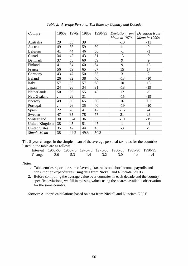
Table 2. Average Personal Tax Rates by Country and Decade

Country 1960s 1970s 1980s 1990-95 Deviation from Mean in 1970s

Deviation fromMean in 1990s

Australia 29 35 39 . -10 -11 Austria 49 55 59 59 11 9 Belgium 41 44 46 50 -1 -1 Canada 34 42 43 51 -3 0 Denmark 37 53 60 59 9 9 Finland 41 54 60 64 9 13 France 56 59 65 67 15 17 Germany 43 47 50 53 3 2 Ireland 26 32 38 40 -13 -10 Italy 57 55 57 68 10 18 Japan 24 26 34 31 -18 -19 Netherlands 50 56 55 45 12 -5 New Zealand . 29 31 . -15 -19 Norway 49 60 65 60 16 10 Portugal . 26 35 40 -19 -10 Spain 22 28 41 47 -16 -4 Sweden 47 65 78 77 21 26 Switzerland 30 324 36 35 -10 -15 United Kingdom 38 45 51 47 1 -4 United States 35 42 44 45 -3 -5 Simple Mean 38 44.2 49.3 50.3

The 5-year changes in the simple mean of the average personal tax rates for the countries listed in the table are as follows:

Interval 1960-65 1965-70 1970-75 1975-80 1980-85 1985-90 1990-95 Change 3.0 5.3 1.4 3.2 3.0 1.4 -.4 Notes:

1. Table entries report the sum of average tax rates on labor income, payrolls and consumption expenditures using data from Nickell and Nunciata (2001).

2. Before computing the average value over countries in each decade and the country-specific deviations, we fill in missing values using the nearest available observation for the same country.

Source: Authors’ calculations based on data from Nickell and Nunciata (2001).

56

Table 3. Cross-Country Regressions of Work Hours and Employment Rates on Tax Rates, 1995 Data

Independent Variable: Sum of tax rates on income, payrolls and consumption

Dependent Variable

Sample

Source for Tax Rates

Slope Coef-ficient

StandardError

P-Value

Adj.

2R Annual Work Hours Per Adult

A Nickell & Nunciata

-6.7 3.3 .07 .21

Annual Work Hours Per Adult

C Nickell & Nunciata

-7.4 2.6 .01 .27

Annual Work Hours Per Adult

D Nickell & Nunciata

-4.1 4.0 .32 .01

Annual Work Hours Per Adult

D Schneider -9.5 2.4 .00 .52

Annual Hours Per Employed Adult

A Nickell & Nunciata

-6.5 2.1 .01 .42

Annual Hours Per Employed Adult

C Nickell & Nunciata

-6.5 2.6 .02 .23

Annual Hours Per Employed Adult

D Nickell & Nunciata

-3.9 3.4 .28 .02

Annual Hours Per Employed Adult

D Schneider -4.9 2.9 .11 .13

100 ×Employment-Population Ratio

A Nickell & Nunciata

-.12 .19 .54 -.05

100 ×Employment-Population Ratio

C Nickell & Nunciata

-.17 .15 .29 .01

100 ×Employment-Population Ratio

D Nickell & Nunciata

-.07 .25 .77 -.08

100 ×Employment-Population Ratio

D Schneider -.38 .19 .07 .19

Notes:

1. All regressions are by ordinary least squares. 2. The “P-Value” reports the marginal significance level in a test of the null hypothesis

that the coefficient on the tax variable equals zero.

Source: Authors’ calculations.

57

Table 4. Panel Regressions of Work Hours and Employment Rates on Tax Rates

Independent Variable: Sum of tax rates on income, payrolls and consumption

Dependent Variable

Sample

Years

Year Effects

CountryEffects

Slope Coeff.

St. Err.

P-Value

Adj. 2R

Annual Work Hours Per Adult

A 77, 83 90, 95

No No -3.1 1.7 .07 .04

Annual Work Hours Per Adult

A 77, 83 90, 95

Yes Yes -4.3 3.0 .16 .83 (.03)

Annual Hours Per Employed Adult

A 77, 83 90, 95

No No -9.1 1.0 .00 .61

Annual Hours Per Employed Adult

A 77, 83 90, 95

Yes Yes -2.2 1.9 .25 .89 (.01)

100 ×Employment-Population Ratio

A 77, 83 90, 95

No No .17 .08 .05 .05

100 ×Employment-Population Ratio

A 77, 83 90, 95

Yes Yes -.21 .13 .09 .88 (.05)

100 ×Employment-Population Ratio

B 1977-1994

No No .15 .04 .00 .05

100 ×Employment-Population Ratio

B 1997-1994

Yes Yes -.22 .04 .00 .94 (.08)

Notes:

1. All regressions are by ordinary least squares, with and without fixed effects, as indicated.

2. The tax rate variable is from Nickell and Nunciata (2001). 3. The rightmost column reports in parentheses the adjusted 2R value after sweeping out

the fixed effects.

Source: Authors’ calculations.

58

Table 5: Cross-Country Regressions of Industry Shares on Tax Measures

Dependent Variable: Percentage of Employment or Value Added in the Industry Group A. Employment Shares Regressed on Tax Measures Industry Group

Sample

Tax Measure

Slope Coeff.

StandardError

P-Value

Adj. 2R

Trade, Repairs, Eating, Drinking, Lodging

E Sum of Rates

-.198 .038 .00 .67

Trade, Repairs, Eating, Drinking Lodging

E Tax Factor

-9.6 2.5 .00 .52

Eating, Drinking and Lodging

E Sum of Rates

-.095

.026 .00 .49

Eating, Drinking and Lodging

E Tax Factor

-5.4 1.3 .00 .55

Retail Trade and Repairs F Sum of Rates

-.055 .025 .07 .32

Retail Trade and Repairs F Tax Factor

-2.8 1.2 .06 .34

B. Value Added Shares Regressed on Tax Measures Industry Group

Sample

Tax Measure

Slope Coeff.

Standard.Error

P-Value

Adj. 2R

Trade, Repairs, Eating, Drinking, Lodging

E Sum of Rates

-.142 .069 .06 .20

Trade, Repairs, Eating, Drinking Lodging

E Tax Factor

-7.4 3.8 .07 .18

Eating, Drinking and Lodging

E Sum of Rates

-.044 .021 .06 .20

Eating, Drinking and Lodging

E Tax Factor

-2.7 1.1 .03 .29

Retail Trade and Repairs F Sum of Rates

-.100 .029 .01 .57

Retail Trade and Repairs F Tax Factor

-5.3 1.3 .00 .67

C. Value Added Share Regressions, Excluding Canada and the United States in Sample E Industry Group

Tax Measure Slope Coeff.

Standard.Error

P-Value

Adj.2R

Sum of Rates -.103 .066 .15 .12 Trade, Repairs, Eating, Drinking, Lodging Tax Factor -4.8 3.5 .20 .08 D. Manufacturing Employment Shares Regressed on Tax Measures in Sample E Industry Group

Tax Measure Slope Coeff.

Standard.Error

P-Value

Adj.2R

Sum of Rates .027 .058 .66 -.07 All Manufacturing Industries Tax Factor 1.7 3.2 .59 -.06

Note: Tax rate measures calculated from data in Schneider (2002). See, also, notes to Table 3. Source: Authors’ calculations and statutory tax rates.

59

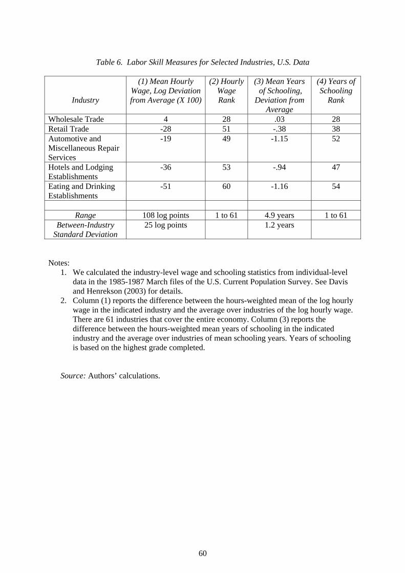
Table 6. Labor Skill Measures for Selected Industries, U.S. Data

Industry

(1) Mean Hourly Wage, Log Deviation from Average (X 100)

(2) Hourly Wage Rank

(3) Mean Years of Schooling,

Deviation from Average

(4) Years of Schooling

Rank

Wholesale Trade 4 28 .03 28 Retail Trade -28 51 -.38 38 Automotive and Miscellaneous Repair Services

-19 49 -1.15 52

Hotels and Lodging Establishments

-36 53 -.94 47

Eating and Drinking Establishments

-51 60 -1.16 54

Range 108 log points 1 to 61 4.9 years 1 to 61

Between-Industry Standard Deviation

25 log points 1.2 years

Notes:

1. We calculated the industry-level wage and schooling statistics from individual-level data in the 1985-1987 March files of the U.S. Current Population Survey. See Davis and Henrekson (2003) for details.

2. Column (1) reports the difference between the hours-weighted mean of the log hourly wage in the indicated industry and the average over industries of the log hourly wage. There are 61 industries that cover the entire economy. Column (3) reports the difference between the hours-weighted mean years of schooling in the indicated industry and the average over industries of mean schooling years. Years of schooling is based on the highest grade completed.

Source: Authors’ calculations.

60

Table 7. Cross-Country Regressions of Shadow Economy Size on Tax Rates Dependent Variable: Shadow Economy as a Percentage of Official GDP Independent Variable: Sum of tax rates on labor income, payrolls and consumption

Source for Tax Rates

Sample

Shadow Economy Measure

Slope Coef-ficient

Standard Error

P-Value

Adj.

2R Nickell and Nunciata

C Currency Demand

.20 .08 .02 .25

Nickell and Nunciata

D Currency Demand

.25 .11 .04 .26

Schneider D Currency Demand

.30 .08 .00 .53

Schneider D Currency Demand (1996)

.31 .08 .00 .53

Nickell and Nunciata

D Electricity Method (1990)

-.04 .11 .75 -.07

Schneider D Electricity Method (1990)

.16 .09 .09 .15

Notes:

1. Data on the size of the shadow economy are averages of 1994 and 1995 values unless otherwise indicated.

2. For the shadow economy size measure based on the Electricity Method, the results are nearly identical whether we use the Nickell-Nunciata tax measure for 1990 or 1995.

3. As explained in the text, the regressions that rely on the Currency Demand Method have a different interpretation than the ones that rely on the Electricity Method.

See, also, notes to Table 3.

Source: Authors’ calculations.

61

Table 8. Cross-Country Regressions with Controls for other Policies and Institutions

A. Control Variable: Ratio of Minimum to Average Wages in 1991-1994 Tax Variable Ratio of Minimum

to Average Wages F-test P-Value

Adj. 2R

Dependent Variable Sample Coeff. S.E. Coeff. S.E. Work Hours Per Adult D -9.5 2.9 .08 3.4 .01 .48 Shadow Economy Size D .19 .10 -.08 .12 .21 .11 Broad Emp. Share E -8.2 3.0 -.06 .07 .01 .51 Broad VA Share E -9.0 4.8 .07 .11 .19 .13 Emp. Share in Eating, Drinking, Lodging

E -5.3 1.7 -.00 .04 .01 .51

VA Share in Eating, Drinking Lodging

E -3.0 1.4 .01 .03 .09 .23

Emp. Share in Retail F -2.9 1.6 .00 .04 .19 .23 VA Share in Retail F -6.6 1.3 .06 .03 .01 .75 B. Control Variable: Percentage of Workers Covered by Collective Bargaining Agreements in 1994 (earlier for some countries) Tax Variable Collective Bar-

gaining Coverage F-test P-Value

Adj. 2R

Dependent Variable Sample Coeff. S.E. Coeff. S.E. Work Hours Per Adult D -9.3 5.1 -.10 2.6 .01 .48 Shadow Economy Size D .17 .18 -.00 .10 .26 .07 Broad Emp. Share E -2.8 3.9 -.08 .04 .00 .63 Broad VA Share E -0.2 6.6 -.08 .06 .09 .24 Emp. Share in Eating, Drinking, Lodging

E -4.4 2.5 -.01 .02 .01 .52

VA Share in Eating, Drinking Lodging

E -1.8 2.0 -.01 .02 .09 .24

Emp. Share in Retail F -0.7 2.1 -.02 .02 .11 .37 VA Share in Retail F -4.4 2.4 -.01 .02 .02 .63 C. Control Variable: OECD Index of Employment Protection Legislation in the late 1990s Tax Variable Index of Employ-

ment Protection F-test P-Value

Adj. 2R

Dependent Variable Sample Coeff. S.E. Coeff. S.E. Work Hours Per Adult D -5.8 3.0 -80.8 44.4 .00 .60 Shadow Economy Size D .13 .12 0.7 1.8 .24 .09 Broad Emp. Share E -7.7 3.0 -0.9 0.9 .01 .53 Broad VA Share E -7.8 4.9 0.2 1.4 .22 .10 Emp. Share in Eating, Drinking, Lodging

E -4.9 1.7 -0.3 0.5 .01 .52

VA Share in Eating, Drinking Lodging

E -2.5 1.4 -0.1 0.4 .10 .23

Emp. Share in Retail F -3.3 1.5 0.3 0.5 .15 .29 VA Share in Retail F -6.2 1.5 0.5 0.4 .01 .68

62

D. Control Variable: Index of Competition-Retarding Product Market Regulations, 1997-98 Tax Variable Index of Product

Market Regulations F-test P-Value

Adj. 2R

Dependent Variable Sample Coeff. S.E. Coeff. S.E. Work Hours Per Adult D -8.4 2.5 -140 102 .01 .55 Shadow Economy Size D .18 .10 -2.2 4.3 .23 .09 Broad Emp. Share E -8.8 2.2 -3.8 1.8 .00 .63 Broad VA Share E -7.5 4.0 0.4 3.3 .22 .10 Emp. Share in Eating, Drinking, Lodging

E -5.0 1.2 -1.8 1.0 .00 .61

VA Share in Eating, Drinking Lodging

E -2.6 1.2 -0.5 0.9 .09 .24

Emp. Share in Retail F -2.6 1.2 -1.1 1.1 .12 .35 VA Share in Retail F -5.6 1.2 1.6 1.0 .01 .73 Notes:

1. All regressions by OLS. For regressions with annual work hours per adult or shadow economy size as the dependent variable, the tax variable is the sum of tax rates on payrolls, labor incomes and consumption expenditures. The share regressions use the tax factor. Both tax variables are based on data from Schneider (2002). The measure of shadow economy size is based on the Electricity Method.

2. Means (standard deviations) for the control variables in Sample D: ratio of minimum to average wages, 51 (11); percentage of workers covered by collective bargaining agreements, 72 (25); index of employment protection, 1.95 (.87); index of product market regulations, .58 (.29). See Table 1 for descriptive statistics of all other variables.

Sources: Authors’ calculations. Minimum wage variable: Nickell and Layard (1999, Table 9) and Dolado et al. (1996, Table 1). Bargaining coverage: Blau and Kahn (1999, Table 2); value for Ireland set to the mean in the top third of the coverage values in Blau and Kahn based on description in Glyn (2002, page 6). Index of employment protection legislation: summary indicator of “Overall EPL Strictness, Version 2”, as reported in OECD (1999, Table 2.5). Index of product market regulations: “Total Product Market, O-NSB Scores”, as reported in Table 1 of Nicoletti and Pryor (2001).

63

Figure 1: Tax Rates and Annual Work Hours Per AdultSample D: 14 Countries in 1995

us

uk

sz

sw

sp

no

ne

it

ir ge

fr

de

ca

be

800

900

1000

1100

1200

1300

1400

35 40 45 50 55 60 65 70 75 80 85

Labor + Payroll + Consumption Tax Rate

Hours

Tax Data from Schneider (2002)

Hours = 1655 - 9.5*(Sum of Tax Rates) (2.4)

64

Figure 2: Tax Rates and Annual Hours Per Employed PersonSample A: 13 Countries with Data for 1977, 1983, 1990 and 1995

ususus

us

ukuk

uk

uk

sw

swsw

sw

spsp

sp

sp

nono

no

no

ja

ja

jaja

itit

itit

ir

iririr

fr

fr

fr

fr

fi fi

fifi

cacaca

ca

be

bebebe

atatat

at

1300

1400

1500

1600

1700

1800

1900

2000

2100

2200

20 30 40 50 60 70 80 90

Labor + Payroll + Consumption Tax Rate

Hours

Tax Data from Nickell and Nunciata (2001)

Hours = 2230 - 9.1*(Sum of Tax Rates) (1.0)

65

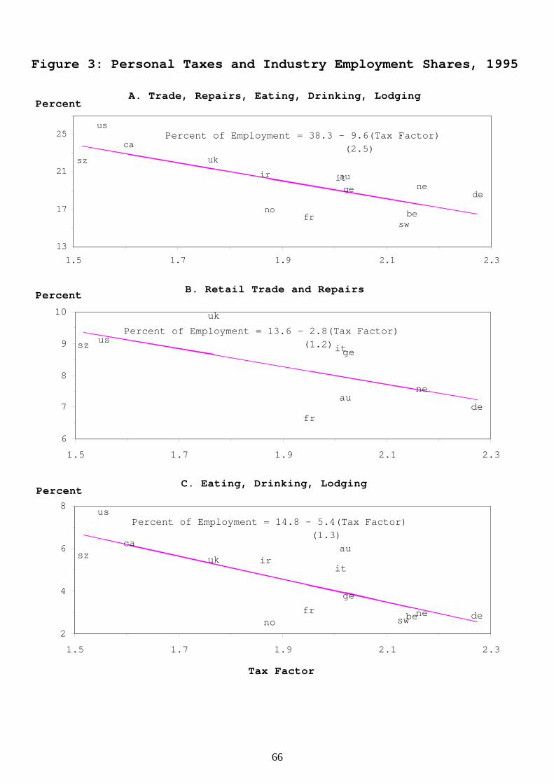
A. Trade, Repairs, Eating, Drinking, Lodging

au

be

ca

de

fr

ge

ir itne

no

sw

sz uk

us

13

17

21

25

1.5 1.7 1.9 2.1 2.3

Percent

Percent of Employment = 38.3 - 9.6(Tax Factor) (2.5)

B. Retail Trade and Repairs

aude

fr

geit

ne

sz

uk

us

6

7

8

9

10

1.5 1.7 1.9 2.1 2.3

Percent

Percent of Employment = 13.6 - 2.8(Tax Factor) (1.2)

C. Eating, Drinking, Lodging

us

uksz

swnone

itir

ge

fr de

ca

be

au

2

4

6

8

1.5 1.7 1.9 2.1 2.3

Tax Factor

Percent

Percent of Employment = 14.8 - 5.4(Tax Factor) (1.3)

Figure 3: Personal Taxes and Industry Employment Shares, 1995

66

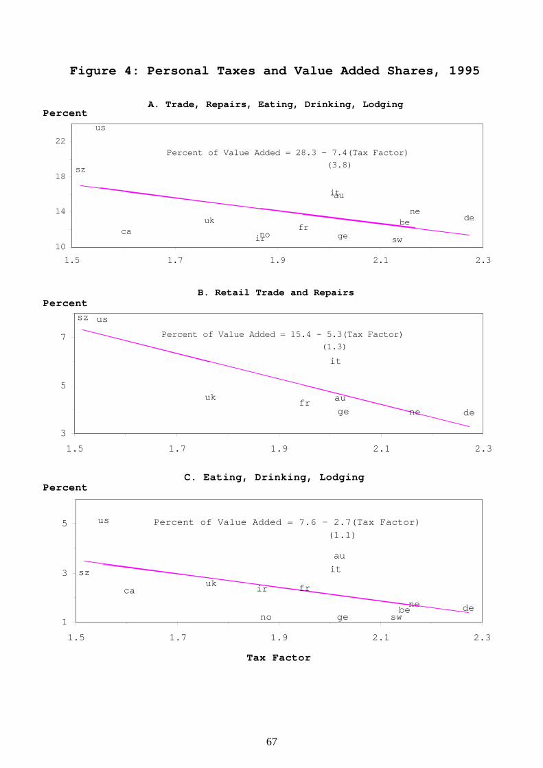
C. Eating, Drinking, Lodging

us

uksz

swnone

it

ir

ge

fr

de

ca

be

au

1

3

5

1.5 1.7 1.9 2.1 2.3

Tax Factor

Percent

Percent of Value Added = 7.6 - 2.7(Tax Factor) (1.1)

A. Trade, Repairs, Eating, Drinking, Lodging

au

beca

defr

geir

it

ne

no sw

sz

uk

us

10

14

18

22

1.5 1.7 1.9 2.1 2.3

Percent

Percent of Value Added = 28.3 - 7.4(Tax Factor) (3.8)

B. Retail Trade and Repairs

au

defr

ge

it

ne

sz

uk

us

3

5

7

1.5 1.7 1.9 2.1 2.3

Percent

Percent of Value Added = 15.4 - 5.3(Tax Factor) (1.3)

Figure 4: Personal Taxes and Value Added Shares, 1995

67

Figure 5: Tax Rates and Shadow Economy as Percent of GDPSample D: 14 Countries in 1995

be

ca

de

frge

ir

it

ne

no

sp

sw

sz

uk

us

6

10

14

18

22

26

30

35 40 45 50 55 60 65 70 75 80 85

Labor + Payroll + Consumption Tax Rate

Percent of GDP

Tax Data from Schneider (2002)

100*(Shadow/GDP) = -2.4 + .3*(Sum of Tax Rates) (.08)

68