NBER WORKING PAPER SERIES

FISCAL POLICY AND MONETARY INTEGRATIONIN EUROPE

Jordi GaliRoberto Perotti

Working Paper 9773http://www.nber.org/papers/w9773

NATIONAL BUREAU OF ECONOMIC RESEARCH1050 Massachusetts Avenue

Cambridge, MA 02138June 2003

Paper prepared for the Economic Policy meeting in Athens, April 2003. We thank the editor GiuseppeBertola, three anonymous referees, Alberto Alesina, Sandro Momigliano, and participants at MacroWorkshops at CREI-UPF and the European University Institute for comments and discussions. We thankGabriele Giudice and Jonas Fischer for providing the European Commission data on fiscal policy. PeterClayes provided excellent research assistance. The views expressed herein are those of the authors and notnecessarily those of the National Bureau of Economic Research.

©2003 by Jordi Gali and Roberto Perotti. All rights reserved. Short sections of text not to exceed twoparagraphs, may be quoted without explicit permission provided that full credit including © notice, is givento the source.

Fiscal Policy and Monetary Integration in EuropeJordi Gali and Roberto PerottiNBER Working Paper No. 9773June 2003JEL No. E32, E62

ABSTRACT

A popular view among economists, policymakers, and the media, is that the Maastricht Treaty and

then Stability and Growth Pact have significantly impaired the ability of EU governments to conduct

a stabilizing fiscal policy and to provide an adequate level of public infrastructure. In this paper, we

investigate this view by estimating fiscal rules for the discretionary budget deficit over the period

1980-2002, using data on EMU countries and control groups of non-EMU EU countries and other

non-EU OECD countries. We do not find much support for this view. In fact, we find that

discretionary fiscal policy in EMU countries has become more countercyclical over time, following

what appears to be a trend that affects other industrialized countries as well. Similarly, we find that

the decline in public investment experienced over the last decade by EMU countries is part of a

world-wide trend that started well before the Maastricht Treaty was signed.

Jordi Gali Roberto PerottiCentre de Recerca en European University InstituteEconomia Internacioanl (CREI) roberto.perotti@iue.itUniversitat Pompeu FabraRamon Trias Fargas 2508005 Barcelona Spainand NBERjordi.gali@crei.upf.es

1. Introduction The fiscal apparatus of the European Monetary Union – as embedded in the Maastricht

Treaty (MT) and the Stability and Growth Pact (SGP)1 – is increasingly regarded by many

as an unnecessary and harmful straightjacket on national fiscal policies, or even as

downright ‘stupid’.2 The SGP, the argument goes, constraints the use of fiscal policy

precisely when countries need it the most, because of the loss of an autonomous monetary

policy. In particular, critics complain that the ceiling of a three percent deficit/GDP ratio

may become dangerously harmful during downturns, since the government’s efforts to

meet that target by cutting spending and raising taxes may only aggravate the recession.

More generally, and given that the SGP fiscal targets are expressed in terms of the size of

deficits unadjusted for cyclical conditions, the need to stabilize the budget over the cycle

may be conducive to a procyclical fiscal policy, i.e., one which may unnecessarily increase

the amplitude and persistence of economic fluctuations in EMU countries.

A second criticism frequently levelled at the MT and the SGP is that they have

impaired the ability of EMU countries to maintain and increase the public capital stock,

which could have possible long-run consequences on the growth potential of these

countries that go well beyond their implications for the cyclical properties of fiscal policy.

Thus, our first objective in the present paper is to evaluate to what extent have the

constraints associated with the MT and the SGP affected in practice the way national

governments have conducted fiscal policy. More specifically, we ask whether and how

those constraints may have made fiscal policy in EMU countries effectively more

procyclical (or, equivalently, less countercyclical). The second objective is to assess

empirically whether the alleged negative effects of the MT and SGP on public investment

can indeed be seen in the data.

Regarding the cyclical behaviour of fiscal policy, we put forward two basic

hypothesis, to be validated or refuted by the data. The first hypothesis, often associated

with the criticisms mentioned above, can be stated as follows: as a result of the constraints

imposed by the MT and the SGP, national fiscal policies can no longer fulfil the stabilizing

role they had traditionally played; this, combined with the loss of an autonomous national 1 In section 2 below we describe briefly some key institutional aspects of the Maastricht Treaty and of the Stability and Growth Pact. For other detailed accounts we refer the interested reader to European Commission (2000) and European Central Bank (1999). Artis and Buti (2000), Buiter, Corsetti and Roubini (1993), Buiter and Grafe (2002), Buti and Giudice (2002), and Eichengreen and Wyplosz (1998) also provide good discussions of the institutional aspects of the Maastricht Treaty and of the Stability and Growth Pact, and detailed economic analyses of their rationale and impact.

1

monetary policy, may result in more aggregate instability, and the risk of more prolonged

recessions.

An alternative hypothesis on the evolution of fiscal policy in EMU countries

stresses the impact of the loss of an autonomous monetary policy. According to this view,

the emergence of the common monetary policy, with a clear mandate to focus on price

stability in the Euro area as a whole, leaves the objective of stabilization of national

business cycles exclusively in the hands of national fiscal authorities. As a result, we

should expect the process of monetary integration, initiated with the MT, to be associated

with more strongly countercyclical fiscal policies in EMU countries.

In order to evaluate the validity of the above hypotheses we estimate empirical

fiscal policy rules for eleven EMU countries over the period 1980-2002. More precisely,

we split that sample period into two sub-periods (pre- and post- Maastricht) and perform a

variety of tests for stability of the coefficient capturing the fiscal response to output gap

fluctuations. Our analysis for EMU countries is supplemented with an analogous exercise

for the three EU countries that did not join EMU, as well as for five OECD countries

which do not belong to the EU; both sets of countries act as control groups for our analysis.

We also devote special attention to the role played by public investment in those changes.

From a methodological point of view, our empirical approach attempts to overcome

some of the weaknesses of earlier work that has attempted to estimate similar fiscal policy

rules. First, we restrict our analysis to measures that can be reasonably interpreted as

indicators of discretionary fiscal policy, i.e. the component of fiscal policy whose

variations do not result from the automatic influence of the cycle or other non-policy

influences. Second, we recognize the potential endogeneity of our cyclical indicators with

respect to exogenous fiscal shocks, which leads us to use an instrumental variables

procedure, with carefully chosen instruments.

To preview some of our conclusions, we detect very little evidence that the

Maastricht-related constraints have significantly impaired in practice the stabilization role

of fiscal policy in EMU countries. If anything, we find evidence for the opposite: EMU

countries’ fiscal policy in the pre-Maastricht period seems to have been significantly

procyclical, a puzzling feature which largely disappears during the post-Maastricht period.

Overall, we detect what appears to be a global trend towards more countercyclical fiscal

policies. Interestingly, however, EMU countries seem to lag behind the rest of OECD

2 Interview to Romano Prodi in Le Monde, 17 October 2002.

2

countries in terms of that trend. Whether the latter observation is a consequence of the MT

and SGP constraints or other factors, it may be still be too early to tell.

Regarding the effects of the MT and SGP on public investment, we find that the

decline in government investment as a share of total spending appears to be a global trend

that started well before Maastricht; in fact, in the post-Maastricht period government

investment declined less than in the eighties, and less in EMU countries than in the other

OECD countries.

The paper is organized as follows. Section 2 presents some institutional background

on the fiscal policy constraints established by the Maastricht Treaty and the Stability and

Growth Pact: the reader already familiar with these issues might want to skip this section.

Section 3 summarizes the evolution of debt and deficit measures in EMU countries,

together with countries in the two control groups, over the past two decades. Section 4

describes the indicators of discretionary fiscal policy used in the rest of the paper, and the

procedures to construct them. Section 5 contains the central exercise of the paper: an

empirical exploration of the practical consequences of the MT and the SGP on the cyclical

properties of discretionary fiscal policy. Section 6 discusses some possible

counterarguments to our interpretation of this exercise. Section 7 presents some descriptive

statistics on the evolution of public investment in the EMU and the other OECD countries.

Section 8 concludes.

2. Institutional Background

The Maastricht Treaty and, subsequently, the Stability and Growth Pact established certain

targets on the size of debt and deficits and other obligations, in order to qualify for EMU

membership and, for those already in EMU, to achieve and maintain “sound” budgetary

positions and avoid harsh penalties.

Art. 104 (ex Art. 104c) of the Treaty establishes that “member sates shall avoid

excessive government deficits” (par. 1), and that compliance with budgetary discipline will

be judged on the basis of two criteria (par. 2):

“a) whether the ratio of the planned or actual government deficit to gross domestic product

exceeds a reference value, unless:

- either the ratio has declined substantially and continuously and reached a level that comes

close to the reference value;

3

- or, alternatively, the excess over the reference value is only exceptional and temporary

and the ratio remains close to the reference value

(b) whether the ratio of government debt to gross domestic product exceeds a reference

value, unless the ratio is sufficiently diminishing and approaching the reference value at a

satisfactory pace.” As is well known, these two reference values were set at 3 percent and

60 percent, respectively.

The first criterion was also used, among other criteria like price stability, when a

decision was made on which countries would be admitted to stage III of the EMU (the

single currency) in July 1998.

The Stability and Growth Pact was designed to provide concrete content to several

provisions of the Treaty regarding economic policies in the EU. It consists of a Resolution

of the European Council and of two ECOFIN Council Regulations (No. 1466/97 and No.

1466/97).

The Resolution reaffirms the commitment to fiscal discipline and introduces the

notion of “medium-term budgetary objective of positions close to balance or in surplus”,

to be respected by member states, in order to “allow all Member States to deal with normal

cyclical fluctuations while keeping the government deficit within the reference value of 3

% of GDP.”

Regulation No. 1466/97 clarifies the procedures to be followed for an

implementation of the surveillance of the Pact, as envisioned in general terms in Art. 99

(ex Art. 103) of the Treaty. In particular, it establishes that

1. member states must submit every year an update to the stability programme (called

convergence programme for non-EMU members), containing a medium-term objective

for the budgetary position, and a description of the assumptions and of the main

economic policy measures the country intends to take to achieve the targets.

2. The Council, on a recommendation from the Commission, delivers and opinion on each

programme and its yearly updates and, if deemed necessary, a recommendation. There are

three possible types of recommendations. First, a recommendation that the programme be

adjusted if deemed defficient in some respect. Second, if after approving the programme

the Council identifies a “significant divergence of the budgetary position from the

medium-term budgetary objective, or the adjustment path towards it”, the Commission can

issue a recommendation (early warning), in accordance with Article 103(4). Third, if the

divergence persists, the Council can issue a recommendation to take corrective action, and

can make the recommendation public.

4

Regulation 1467/97 first tries to make more precise the notion of “exceptional and

temporary” excess of the deficit over the 3% of GDP threshold, as introduced by Article

104 (ex Article 104c) of the Treaty. Article 2(1) of the regulation specifies that an

“exceptional and temporary” excess of the deficit is allowed “when resulting from an

unusual event outside the control of the Member State concerned and which has a major

impact on the financial position of the general government or when resulting from a severe

economic downturn.” Articles 2(2) and 2(3) further specify that a deficit will be considered

exceptional “if there is an annual fall of real GDP of at least 2 %” or if a member state can

argue successfully that the circumstances are “exceptional”, based on “the abruptness of

the downturn or on the accumulated loss of output relative to past trends”. The Regulation

then clarifies the Excess Deficit Procedure set out in Article 104 (ex Art 104c) of the

Treaty, including the imposition of fines.

Thus, for our purposes the key elements of the SGP can be summarized as follows:

- Each country must state and abide by a set of medium-term objectives, including a

budgetary position “close to balance or in surplus”.

- A clarification of the circumstances that trigger an early warning.

- A clarification of the Excess Deficit Procedure, and in particular of the

circumstances under which a deficit in excess of 3% of GDP is allowed.

In spite of all these attempts at clarification, there are many aspects of the SGP which

remain ambiguous. In turn, this might have an impact on the actual stringency of the

provisions of the pact. We stress three such areas of ambiguity:

1. What is a “medium-term target”? The SGP is not entirely clear on this. Initially,

the expression “sound budgetary positions close to balance or in surplus” was operationally

identified with the “minimal benchmark”, i.e. a position such that, if the country were

subject to a “worst-case scenario”, the budget deficit would still be less than 3% of GDP if

the automatic stabilizers were allowed to operate. As such, the notion of “minimal

benchmark” is bound to be subjective and controversial. The Commission computes the

minimal benchmark for each country based on two pieces of information: the worst-case

scenario for the output gap, and the sensitivity of the budget to GDP. Operationally, the

former is taken to be the largest negative output gap since 1960, or two times the standard

deviation of the output gap (see for example European Commission (1999), p. 4).

However, the revised Code of Conduct on the content and format of the stability

and convergence programmes, endorsed by the ECOFIN Council in 2001, introduced a

clarification to the notion of medium-term targets, requiring additional margins to cope

5

with unforeseen budgetary risks and to reduce high debts. Thus, the safety margin as

embodied in the minimal benchmarks –already an ambiguous concept-- no longer seems to

constitute automatic compliance with the “sound budgetary position” envisioned in the

Treaty.

The new Code of Conduct also introduces a distinction between the notions of

“appropriate medium-term target” and the notion of “close to balance or in surplus” which

constitutes the key obligation of the SGP. It provides that a stricter goal than close to

balance might be justified in view of several considerations, like providing for the costs of

an ageing population, to create rooms for discretionary fiscal policies, etc. (see European

Commission (2002), p. 33) .

2. The SGP does not say how to identify an “actual or expected significant

divergence of the budgetary position from the medium-term budgetary objective”, which

could trigger an early warning. There is a growing consensus that, at a minimum, the

cyclically adjusted budget balance should be used in making this assessment (indeed, that

the whole SGP should be reformulated in terms of cyclically adjusted balances). The SGP

does not refer to cyclically adjusted balances. However, the new Code of Conduct states

that “..cyclically adjusted balances should continue to be used, in addition to nominal

balances, as a tool when assessing the budgetary position.” Indeed, the 2002 Council

Opinions on the programmes of six member mentions the notions of cyclically adjusted

balances. But the implications of this acknowledgment are far from clear. For instance, the

2002 Council Opinion on Greece states “the budgetary projections remain in surplus

throughout the period of the programme in both actual and cyclically adjusted terms”. In

2003, it writes that “in 2006 there may still be a small cyclically adjusted government

deficit.” These are the only references to cyclical adjustment in the Council Opinions on

Greece.

3. The SGP does not specify exactly what constitutes the “exceptional

circumstances” that define a “severe” recession when GDP falls by less than 2%, and

which might exempt a country from the 3% deficit limit for an unspecified period of time.

This makes the SGP and the Excess Deficits Procedure prone to endless bargaining and

controversy.

6

3. Debts and Deficits: the Record

To provide some background, we start by looking at a few descriptive statistics on the

medium-term evolution of the size of debt and deficits in the current EMU countries, as

well as in two control groups: the three EU countries which do not belong to the EMU

(Denmark, UK, and Sweden; henceforth, the EU3 countries for short), and five non-EU

OECD countries for which we were able to assemble a consistent dataset of budget data

(Norway, Australia, Japan, Canada, US; henceforth the OECD5, for short). It is not

obvious that Denmark, the UK, and Sweden do in fact constitute an appropriate control

group as they might be considered, prima facie, subject to the provisions of the MT and of

the SGP. In fact, their position is more nuanced (see Box 1): while many provisions of the

MT and of the SGP do apply to them, it is also true that they have less teeth, as these

countries are not subject to penalties in case their deficits exceed 3 percent of GDP.

Box 1: Denmark, Sweden, and the UK

The position of the three non-EMU countries is partly ambiguous. Regulation 1467/97

establishing the SGP states that paragraph 1 of Article 104 (ex Art. 104c) of the Treaty –

“Member States shall avoid excessive government deficits” - does not apply to the United

Kingdom unless it moves to the third stage. However, the United Kingdom is still under

the obligation of paragraph 4 of Article 116 (ex Art. 109e) – “In the second stage, Member

States shall endeavor to avoid excessive government deficits”. The Council has also

interpreted the SGP in the sense that the obligation to pursue a goal of ‘close to balance or

surplus in the medium term’ applies to the UK (see for example the ‘2002 Council

Opinion’ on the updated convergence programme.

In contrast to the United Kingdom, the resolution and the two regulations

establishing the SGP fail to state explicitly that Art. 104(1) does not apply to Denmark. In

fact, the 2002 Council opinion on the updates convergence programme for Denmark states

that “Denmark is also expected to be able to withstand a normal cyclical downturn without

breaching the 3 % of GDP deficit reference value.”

However, both Denmark and the United Kingdom are explicitly exempted from the

requirement of paragraphs 9 and 11 of Article 104 (ex Art. 104c), which establish the right

7

of the Council to request specific actions and to impose non-interest bearing deposits and

fines, in cased of a deficit in excess of 3%.

While Denmark and the United Kingdom have an opt-out from participation in

stage 3 of the EMU (the single currency), technically speaking Sweden only has a

derogation. The practical consequence for the applicability of the SGP, however, appears

to be the same as for Denmark; Art. 122(3) of the Treaty establishes that paragraphs 9 and

11 of Art. 104 do not apply to countries with a derogation.

Columns (a) and (b) in Table 1 display the average deficit/GDP ratio for the above

groups of countries during two different five-year periods (1988-1992 and 1997-2001);

column (c) displays the difference between the first two columns. The first such period

corresponds to the years immediately before the adoption of the MT, whereas the second

sub-period includes the first five years for which the constraints associated with the MT

and/or the SGP were in place.3 The table confirms the well-known substantial decline in

the deficit/GDP ratio in all EMU countries but one (Germany). The average decline in the

deficit/GDP ratio in EMU countries was 4.0 percentage points; Greece had the largest

adjustment – more than 11 percentage points, followed closely by Italy with 9.2 percentage

points.4

To what extent was such a fiscal consolidation restricted to current EMU countries?

Interestingly, a look at the performance of our control groups suggests that sizable

consolidations were also taking place over the same period in non-EMU countries. The

OECD5 group experienced an average decline of 3.2 percentage points in the deficit/GDP

ratio, a decline that becomes much larger (6.0 percentage points) if one excludes Japan.

The EU3 group shows a smaller reduction in the deficit/GDP ratio, about 0.8 percentage

points; this can largely be explained by the much more favorable initial position, an

average deficit ratio of 0.7 % in the 88-92 subperiod.

One interpretation of the above evidence is that, while the MT and SGP may have

provided political cover and hence facilitated the necessary adjustments in EMU countries,

the economic rationale for fiscal consolidation may lie beyond the requirements for

monetary union: the substantial fiscal consolidations experienced by EMU countries in the

3 The decision about the set of countries qualifying to join EMU from its birth in 1999 was made in May 1998 on the basis of 1997 fiscal figures, among other factors. Greece is an exception since it did not join EMU until 200x. 4 The only outlier among EMU countries, Germany, experiences a small increase of 0.2 percentage points (albeit starting from the lowest deficit ratio among EMU countries, 1.9% in the early sub-period).

8

90s can be seen as part of a global trend among industrialized countries (with Japan as a

major outlier), and hence not restricted to the would-be EMU countries.

A look at the evolution of the debt/GDP ratios suggests a good reason for these

worldwide fiscal consolidations. The last three columns in Table 1 show the value of that

ratio in three selected years (1982, 1992, and 2001) points to the non-sustainability of the

fiscal position that most industrialized countries were maintaining in the 80s. In particular,

the average debt/GDP ratio for current EMU members increased from 48 % to 74%

between 1982 and 1992, and from 52% to 62% among the OECD5 countries. Only the

EU3 countries, which started their fiscal consolidation process at an earlier stage, managed

to contain the rise in the debt/GDP ratio to only 3 percentage points, from 58% to 61%. It

has been only after the fiscal consolidations of the 90s that most industrialized countries

began to experience a decline or at least a deceleration in their debt/GDP ratios.

4. Measures of Discretionary Fiscal Policy

In order to study the issues set out in the introduction we first need to distinguish

between changes in fiscal policy that are due to discretionary measures taken by

policymakers, and those that are due to the “automatic” response of fiscal variables to

business cycle fluctuations.

We can think of the budget deficit in a given year as the sum of a “cyclical” and a

“structural” component.

1) The “cyclical” or “non-discretionary” deficit is the component of the latter

whose variations are due (at least in the short run) to causes outside the direct control of

the fiscal authorities, like business cycle fluctuations in unemployment and in the tax

bases. In the case of taxes, these variations can be interpreted as changes in tax revenues

due to changes in income, for given tax rates and for given definitions of the tax bases; 5

among primary expenditures, only unemployment benefits probably have a non-negligible

built-in response to output fluctuations. In addition, we can think of debt interest payments

as an element of this component, since they are largely outside the control of the fiscal

authorities.

5 For simplicity, we abstract here from automatic responses to inflation and interest rates. These are more difficult to estimate. For such an attempt, see Fatás and Mihov (2002b), Perotti (2002), and Canzoneri et al. (2002).

9

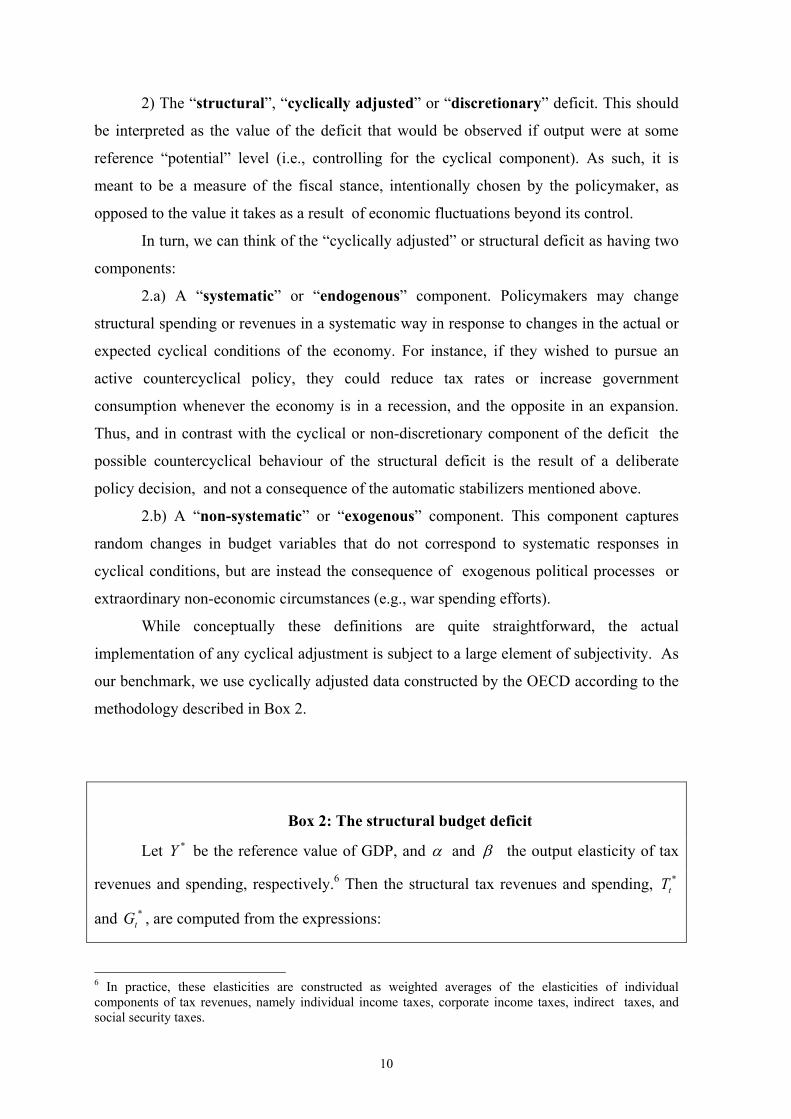
2) The “structural”, “cyclically adjusted” or “discretionary” deficit. This should

be interpreted as the value of the deficit that would be observed if output were at some

reference “potential” level (i.e., controlling for the cyclical component). As such, it is

meant to be a measure of the fiscal stance, intentionally chosen by the policymaker, as

opposed to the value it takes as a result of economic fluctuations beyond its control.

In turn, we can think of the “cyclically adjusted” or structural deficit as having two

components:

2.a) A “systematic” or “endogenous” component. Policymakers may change

structural spending or revenues in a systematic way in response to changes in the actual or

expected cyclical conditions of the economy. For instance, if they wished to pursue an

active countercyclical policy, they could reduce tax rates or increase government

consumption whenever the economy is in a recession, and the opposite in an expansion.

Thus, and in contrast with the cyclical or non-discretionary component of the deficit the

possible countercyclical behaviour of the structural deficit is the result of a deliberate

policy decision, and not a consequence of the automatic stabilizers mentioned above.

2.b) A “non-systematic” or “exogenous” component. This component captures

random changes in budget variables that do not correspond to systematic responses in

cyclical conditions, but are instead the consequence of exogenous political processes or

extraordinary non-economic circumstances (e.g., war spending efforts).

While conceptually these definitions are quite straightforward, the actual

implementation of any cyclical adjustment is subject to a large element of subjectivity. As

our benchmark, we use cyclically adjusted data constructed by the OECD according to the

methodology described in Box 2.

Box 2: The structural budget deficit

Let be the reference value of GDP, and *Y α and β the output elasticity of tax

revenues and spending, respectively.6 Then the structural tax revenues and spending, T *t

and G , are computed from the expressions: *t

6 In practice, these elasticities are constructed as weighted averages of the elasticities of individual components of tax revenues, namely individual income taxes, corporate income taxes, indirect taxes, and social security taxes.

10

* * * *

;t t t t

t t t t

T Y G YT Y G Y

α β

= =

(1)

In other words, in each year the revenue elasticity α is used to evaluate the value revenues

would take if output were at its reference level Y instead of its actual value Y , and *t t

similarly for government spending. Dividing T by the reference value of GDP, * andt*

tG

we obtain the “structural” budget deficit as a share of reference GDP

* *t td g t *

t= − (2)

where are the structural primary deficit, primary revenues, and primary * * *, , andt t td t g

spending, all as shares of reference GDP.

Thus, the output of the structural adjustment depends on the reference value of

GDP used. Typically, this is some measure of smoothed output, like trend or HP-filtered

GDP, or of potential output. In our benchmark results, based on data cyclically adjusted by

the OECD, the reference value of GDP is potential output, constructed following a

standard production function approach (see Giorno et al. (1995) or OECD (2002a)). 7

For robustness we also use different cyclically adjusted fiscal data, computed by

the European Commission and based on two alternative reference GDPs: HP-filtered GDP

and potential output based on the Commission’s production function approach (see

European Commission (2002)). 8

A second source of variation in cyclical adjustment procedures is the elasticities

used. The OECD elasticities are constructed starting from the tax code and the distribution

of taxpayers by income brackets (see Giorno et al. (1995) and van den Noord (2002)). The

same elasticities are used by the European Commission (see European Commission

(2002)).9

Henceforth our empirical analysis focuses on a measure of the structural or

cyclically adjusted primary deficit, which we interpret as an indicator of the fiscal policy

7 The notion of potential output is subject to a large debate of its own. Indeed, any alternative reference value of GDP is open to criticism. We use potential GDP because this is the reference value used by the OECD and the European Commission to cyclically adjust budget figures. 8 The European Commission has just started using potential output in its cyclical adjustment, in addition to HP-filtered GDP, with the November 2002 release of the data. We thank Gabriele Giudice for providing us with the data the very day they were released. 9 Some studies use elasticities estimated from a regression of tax revenues on GDP or the tax base. If taxes have a contemporaneous effect on output (a reasonable assumption with yearly data), the estimates so obtained are inconsistent. This would impair our estimates of the reaction of discretionary fiscal policy to cyclical conditions.

11

stance. 10 As a summary indicator of the cyclical conditions of an economy at any point in

time, we a use a conventional, production function-based output gap measure, also

constructed by the OECD using the same measure of potential output used in the

construction of the cyclically adjusted figures.

5. Has Discretionary Fiscal Policy Changed since Maastricht?

Our objective in the present section is to ascertain the extent to which European

governments have used fiscal policy as a stabilizing tool over the past two decades, and

whether constraints on fiscal policy associated with Maastricht and the SGP may have

hampered their ability and/or motivation to pursue active countercyclical fiscal policies.

5.1. Fiscal Rules

To this end, a natural starting point would be to regress an indicator of fiscal policy

on a cyclical indicator. Several researchers have estimated a relation of the type (see Box 3

for a brief discussion of the recent literature on the subject):

0t x td xφ φ= + + tu

(3)

where dt is the total, cyclically unadjusted deficit as a share of GDP (or spending, or

revenues, or their components) and xt is either the output gap or GDP growth, perhaps with

some additional controls. Such a regression provides a useful descriptive statistic of the

cyclical relation between budget variables and economic activity. However, this regression

would not be a useful starting point in identifying the systematic response of discretionary

fiscal policy to cyclical conditions. The main reason, well understood by now, lies in the

10 We do not have a strong view on what is the appropriate measure of the fiscal stance, whether the level or the change in the deficit. The choice of the indicator of the fiscal policy stance depends very much on the underlying model of the economy and the notion on policy stance one has in mind. For instance, in a simple IS-LM model, the level of the budget surplus determines the position of the IS curve, while the change in the budget surplus determines movements of this curve. Depending on one’s notion, an “expansionary” fiscal policy might be one characterized by a large deficit, or by an increasing deficit. To ease comparability with the literature, we present all our results for the level of the structural surplus. Note that, when we estimate fiscal rules in section 3, the lagged structural surplus appears as an independent variable. Whether the

12

fact that an important component of the budget deficit reflects the automatic, non-

discretionary variations in government revenues and expenditures, as well as variations in

interest payments resulting from changes in interest rates outside the control of the fiscal

authorities.

Using the primary, cyclically adjusted budget deficit as an indicator of the fiscal

policy stance may help in overcoming the previous problem, but it is still unsatisfactory.

The reason is simple: any non-negligible exogenous component in that deficit measure,

reflected in the error term of the fiscal rule, is likely to be (positively) correlated with the

output gap. This correlation, which results from changes in the fiscal policy stance causing

changes in the output gap, will most likely generate an upward bias (and possibly even a

sign switch) in the estimate of xφ , the coefficient on the output gap in the fiscal policy rule.

Clearly, addressing this problem calls for instrumental variable estimation, or,

equivalently, regressing the deficit on a component of the output gap which is uncorrelated

with exogenous discretionary fiscal shocks. This is the approach that we follow below.

An additional problem with a specification of the fiscal policy rule like (3) is that it

might not take properly into account the timing of fiscal policy decisions implied by the

budgetary process of most countries: many discretionary fiscal parameters (e.g., tax rates)

are largely determined the year before they become effective. If this is the case, any policy

rule seeking to respond to output gap variations will have to be based on the expectation of

the latter, conditional on information available in the previous period. In practice, this calls

for replacing tx with in our rule specification. 1tE x− t

*tu

Following the lead of several authors11, we also incorporate a debt stabilization

motive by adding a measure of the size of the debt outstanding (relative to potential GDP)

at the time of the budget decision, and which we denote by bt-1

Finally, we account for the likely autocorrelation of budget decisions (possibly

resulting from gradual adjustment to a target budget, or just from the serial correlation in

the exogenous shocks) by adding the lagged dependent variable as a regressor.

The resulting specification of the fiscal rule that we estimate is thus:

(4) *0 1 1 1t x t t b t s td E x b dφ φ φ φ− − −= + + + +

dependent variable is the level or the difference of the structural surplus, it would then make no difference for the estimate of the other coefficients of the regression. 11 Many authors have incorporated debt measures in empirical fiscal policy rules and examined their relevance to budget decisions. See, e.g., Bohn (1998), Ballabriga and Martinez-Mongay (2002), and Wyplosz (2002).

13

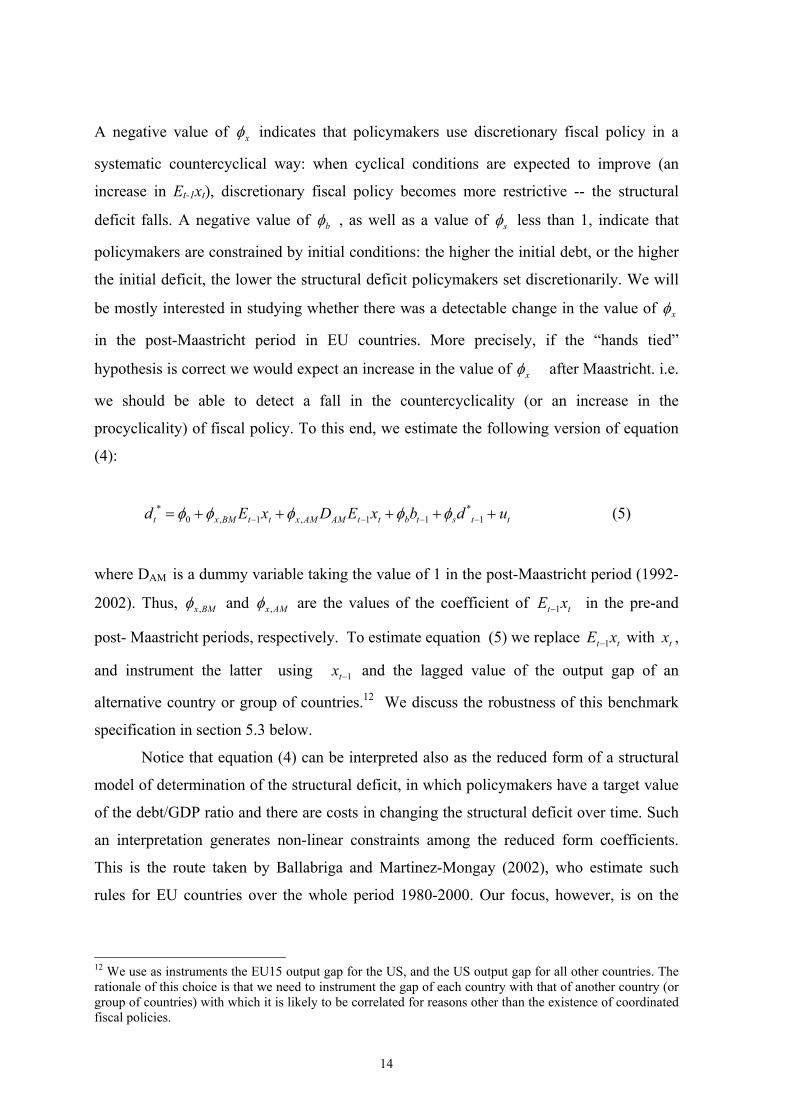
A negative value of xφ indicates that policymakers use discretionary fiscal policy in a

systematic countercyclical way: when cyclical conditions are expected to improve (an

increase in Et-1xt), discretionary fiscal policy becomes more restrictive -- the structural

deficit falls. A negative value of bφ , as well as a value of sφ less than 1, indicate that

policymakers are constrained by initial conditions: the higher the initial debt, or the higher

the initial deficit, the lower the structural deficit policymakers set discretionarily. We will

be mostly interested in studying whether there was a detectable change in the value of xφ

in the post-Maastricht period in EU countries. More precisely, if the “hands tied”

hypothesis is correct we would expect an increase in the value of xφ after Maastricht. i.e.

we should be able to detect a fall in the countercyclicality (or an increase in the

procyclicality) of fiscal policy. To this end, we estimate the following version of equation

(4):

(5)

* *0 , 1 , 1 1 1t x BM t t x AM AM t t b t s td E x D E x b dφ φ φ φ φ− − −= + + + + + tu−

where DAM is a dummy variable taking the value of 1 in the post-Maastricht period (1992-

2002). Thus, ,x BMφ and ,x AMφ are the values of the coefficient of in the pre-and

post- Maastricht periods, respectively. To estimate equation (5) we replace with

1tE x− t

t1tE x− tx ,

and instrument the latter using 1tx − and the lagged value of the output gap of an

alternative country or group of countries.12 We discuss the robustness of this benchmark

specification in section 5.3 below.

Notice that equation (4) can be interpreted also as the reduced form of a structural

model of determination of the structural deficit, in which policymakers have a target value

of the debt/GDP ratio and there are costs in changing the structural deficit over time. Such

an interpretation generates non-linear constraints among the reduced form coefficients.

This is the route taken by Ballabriga and Martinez-Mongay (2002), who estimate such

rules for EU countries over the whole period 1980-2000. Our focus, however, is on the

12 We use as instruments the EU15 output gap for the US, and the US output gap for all other countries. The rationale of this choice is that we need to instrument the gap of each country with that of another country (or group of countries) with which it is likely to be correlated for reasons other than the existence of coordinated fiscal policies.

14

difference between the pre- and post- Maastricht periods, and we also look at revenues and

spending separately.

Box 3: The cyclical sensitivity of fiscal policy

Several recent papers also estimate the cyclical sensitivity of fiscal policy in OECD

countries. There are two main differences with our investigation. First, in all this literature

the fiscal variables are cyclically unadjusted, thus making it impossible to separately

identify the automatic from the discretionary responses of fiscal policy to cyclical

conditions, an issue which is the focus of our analysis. Second, in most papers the

indicator of cyclical conditions is not instrumented, thus preventing a structural

interpretation of the coefficient of the cyclical condition if fiscal policy has a

contemporaneous effect on GDP in yearly data. To facilitate a comparison with our results,

we will discuss these contributions as if their dependent variable were the deficit, although

in most of them it is actually the surplus.

Fatás and Mihov (2002a) and (2002b) regress the (cyclically unadjusted) primary

deficit (or its first difference) on cyclical indicators like the output gap, inflation, and

interest rate, and interpret the residual of this estimated equation as the indicator of the

discretionary fiscal stance. In our terminology, they estimate the ‘non-systematic’

component of discretionary fiscal policy (subject to the caveat above that they do not

instrument for the contemporaneous output gap on the r.h.s.). They show that the average

(across countries) standard deviation of this estimated residual has fallen in the nineties,

and interpret this result as evidence that EU countries have been less able to conduct

countercyclical fiscal policy in the Maastricht years.

Arreaza et al. (1999), Hercowitz and Strawczynski (1999) and Lane (2002)

characterize the cyclical properties of fiscal policy in OECD countries by estimating

similar regressions to Fatás and Mihov (2002a) and (2002b) both on a panel of OECD

countries and on individual countries. These papers also look at how the cyclical behaviour

of fiscal policy is affected by institutional and political factors, and they also disaggregate

the deficit into its main spending and revenue components. Like Fatás and Mihov they use

cyclically unadjusted data; only Lane (2002) instruments the cyclical indicator. Both

Arreaza et al (1999) and Lane (2002) find that the deficit / GDP ratio is countercyclical;

Hercowitz and Strawczynski (1999) show that this is mostly due to recessions; in

expansions, the deficit/GDP ratio is essentially acyclical.

15

A number of papers try to assess the automatic stabilizing properties of fiscal policy.

Melitz (1997) and Wyplosz (1999) estimate similar regressions to Fatás and Mihov on a

panel of European countries (typically including more variables on the r.h.s., in particular

the debt/GDP). They also find and note a countercyclical behaviour of the deficit/GDP

ratio. 13

Wyplosz (2002) regresses the cyclically unadjusted deficit / GDP ratio on the output

gap in 4 countries: USA, UK, Germany, and Italy. His regressions are most closely

comparable to ours because he allows for a break in 1992. The differences in results are

substantial. For instance, in the pre-1992 sample, he finds that the deficit is countercyclical

in USA and Italy, and acyclical in Germany and UK; in contrast, we find that the

structural deficit is essentially acyclical in US, UK and Italy, and procyclical in Germany

(see Table 2 below).

Thus, in general we tend to find a less countercyclical behaviour of the deficit than in

the studies above, particularly in the first part of the sample and for the current EMU

countries. This is easy to explain, since the automatic response of revenues to the cycle

would show up as a countercyclical response of the cyclically unadjusted deficit. These

differences illustrate the importance of distinguishing properly the discretionary and the

cyclical component of the deficit, depending on the purpose of the study.

5.2. Baseline Results

ults for our baseline specification. Initially we estimate

equation (5) over the sample period 1980-2002.14 For each country, the first four columns

of t

Table 2 displays the res

he table display the estimates of ,x BMφ and ,x AMφ , i.e. the coefficients on the expected

output gap in the pre-Maastricht (1980-91) and the post-Maastricht (1992-2002) periods,

respectively, with t-statistics in parent s. The wing column displays the p-value for

the test of the null hypothesis of equality of the output gap coefficients between the two

periods, i.e. , ,x BM x AM

hese follo

φ φ= . The table also reports the estimates of the coefficients on lagged

Our data for the benchmark regression come from the December 2002 issue of the OECD Economic Outlook, hence the figures for 2002 are forecasts based on data available in early fall of 2002.

13 The focus of these papers is twofold: the response of the fiscal instrument to indicators of monetary policy; and the automatic stabilizing properties of fiscal policy. For this reason, Melitz (1997) uses the unforecastable component of the gap, rather than the forecastable component as we implicitly do, to measure the cyclical conditions that affect the contemporaneous deficit. 14

16

debt and defi ir t-statistics. At the bottom average values for the EMU, the EU3,

and the OECD5 groups are shown.

Looking at the averages, in the

cit, with the

tistic

pre-Maastricht period discretionary fiscal policy was

mil15

dly procyclical in EMU countries. By contrast, it was strongly countercyclical in the

EU3 or mildly so in the OECD5, our two control groups. Most interestingly, in all groups

there is a clear trend towards a smaller value of xφ in the post-Maastricht period. On

average, between the two subperiods xφ falls by about 0.5 in EMU and OECD5 countries,

and by 0.3 in EU3 countries.

Notice that only in one country from the EMU group, Greece, does the point estimate

of xφ increase in the second period, indicating a more procyclical discretionary fiscal

policy after Maastricht; however, the difference is far from significant. Among the EU3

countries, only in Denmark and Australia does the point estimate of xφ increase, but again

the difference is entirely insignificant. 16

Thus, there appears to be no evidence of a less countercyclical or more procyclical

disc

too precise

esti

17

retionary fiscal policy in the EMU countries in the post-Maastricht period.

Because of the paucity of degrees of freedom, one should not expect

mates from the country-specific regressions above. In order to overcome this problem

we have also estimated a panel version of our fiscal rule. Table 3 displays the panel

estimates of equation (5), with country fixed effects, for the three groups of countries.

Because we have more degrees of freedom, we can now allow for differences pre- and

post-Maastricht in all the coefficients of the equation (and in the country dummies). For

each of the three groups of countries, the first and second rows display the estimates of the

coefficient on 1t tE x− in the pre- and post- Maastricht periods, respectively, with their

associated t-sta in parentheses. In the third and fourth columns we report the

15 The average of the EU3 countries is highly influenced by the large negative value estimated for Denmark. 16 We also find that the higher initial debt/GDP ratios, the lower the deficit, given last year’s deficit; thus, the debt does exert a constraint on the deficit. In the EMU countries, we typically find that an extra 10 percentage points of debt/GDP ratio is associated with a lower deficit of about .8 percentage points the next year. The coefficient on the lagged discretionary deficit is lower than 1; on average, in the EMU countries, only about 40 percent of an increase in the structural deficit survives the next year, other things equal. 17 Because we have the lagged endogenous variable on the r.h.s., the standard fixed effect estimator of equation (5) is inconsistent. However, we are mostly interested in the difference between the estimates of the coefficients between the two periods. If the ‘inconsistency’ in the estimates were approximately the same in the two subperiods, the difference would be largely unaffected. Because the small-sample properties of the consistent estimators that have been proposed in the literature are not well understood, and our sample size is small (10 years for each period), we have chosen to present results with a standard IV fixed effect estimator.

17

difference between the two sub-periods, and the p-value for the test of no difference. A

similar structure applies to the other rows of Table 3.

The pattern that emerges is very similar to that of the country-specific regressions, but

now

coefficient of debt is negative in the EMU and EU3 groups, but

ess

the two main components of the

bud

the standard errors are considerably smaller. In all groups of countries, there is

evidence of a significant increase in the degree of countercyclicality of discretionary fiscal

policy. In the EMU group, discretionary fiscal policy was procyclical before Maastricht

and becomes essentially acyclical after Maastricht; in the EU3 and OECD5 groups, it was

acyclical before Maastricht and becomes significantly countercyclical after Maastricht. In

all three cases, the p-value of a test of the difference in the output gap coefficient between

the two periods is never higher than 0.04. Notice also that such a difference is close to the

average difference from the country-specific regressions, especially for the EMU and the

OECD5 countries.

The estimated

entially zero in the OECD5 group. In no case is it significantly different across the two

periods. The average EMU country typically reduces the structural deficit by 0.05

percentage points for each additional percentage point of debt in the previous year.18

Similarly, the estimated coefficient on the lagged deficit is very close in all three groups of

countries – between 0.55 and 0.75 --, and again there is no evidence that it has increased

after Maastricht. Thus, we find no evidence that, holding constant the (expected) cyclical

conditions of the economy, in the post-Maastricht period the initial fiscal conditions

exerted a stronger pressure on discretionary fiscal policy.

Table 4 repeats the same exercise as Table 3, but with

get deficit, spending and revenues, used separately as dependent variables. When

cyclically adjusted primary spending is used as a fiscal indicator, the estimated value of xφ

falls for the three group of countries in the post-Maastricht period, but only in the EMU

group is the difference significant at the 10 percent level. On the other hand, when we use

cyclically adjusted primary revenues as the dependent variable, we detect some evidence

of an increase in the output gap coefficient (thus reflecting a more countercyclical policy)

for the EU3 and OECD5 groups (though only at the 0.16 level for the latter), but not for the

EMU countries. Thus, the previous evidence suggests a more important role of spending

policies in EMU as a countercyclical tool in the post-Maastricht or, to be more precise, an

end to their procyclical pattern, which characterized the pre-Maastricht period. In the case

18 Notice that this point estimate is consistent with what we found in the country-specific regressions.

18

of the EU3 and the OECD5 the evidence points to more proactively countercyclical

revenue policies in the post-Maastricht period.

5.3. Robustness

ove, given the substantial uncertainty inherent in any cyclical

adjustm

so far with cyclically adjusted data from

the Eu

focus on the response of discretionary fiscal policy to the indicator of

cyclica

As discussed ab

ent procedure, it is important to make sure that our results are robust to alternative

measures of cyclically adjusted budget variables.

We have replicated all the tables displayed

ropean Commission, and in the two versions now available (based on HP-filtered

GDP or potential output). In all cases, the results are virtually identical to those obtained

with OECD data.

Our results

l conditions relevant for fiscal policy making. Since we have little information on

what the latter actually is, it is also important to experiment with alternative measures.

Thus, we replicated all our tables using the actual growth forecast for year t, made by the

OECD in the fall of year t -1, as a proxy for the anticipated cyclical indicator in the fiscal

rule (5). 19 In this specification, we find an even larger decline in the estimate of xφ in the

post-Maastricht period. In the EMU countries, this coefficient declines by 0.5 points, by

1.3 in the EU3 countries, and by 0.6 in the OECD5 countries. In all cases, that difference is

significant at the 5 percent level.

Note that, if the growth forecasts are “unbiased”, then the regression residual can

now be

viewed as an estimate of the ‘non-systematic’ or ‘exogenous’ component of the

structural deficit. It is interesting to compare the behavior of this residual to the behavior of

a fiscal rule like (3) (therefore, without instrumenting for GDP and with the unadjusted

deficit as dependent variable), estimated by Fatás and Mihov (2002a) and (2002b). They

show that the standard deviation of the residual of this equation has declined in the

nineties, and interpret this finding as evidence that European countries have been less able

to conduct stabilizing fiscal policy. As we discuss above, we believe this conclusion is

unwarranted, because the residual of equation (3) does not have a clear interpretation. In

fact, we also find that the standard deviation of the residual of equation (5), with the OECD

19 We have obtained these forecasts manually from the printed versions of the OECD Economic Outlook. The OECD Economic Outlook has started publishing forecasts of the output gap, as opposed to GDP growth, only in 1995.

19

growth forecast as independent variable, has fallen after Maastricht in EMU countries

(although, interestingly, not in the two other groups). However, as we have seen this is not

inconsistent with discretionary fiscal policy becoming more stabilizing over the same

period. Indeed, the reduction of the standard deviation of the residual of equation (5) can

be interpreted as another sign of improvement in fiscal policy management, in the sense

that discretionary fiscal policy has become less erratic. Interestingly, this is consistent with

similar evidence concerning monetary policy.

We also estimated a backward-looking version of equation (5), where the structural

deficit is assumed to respond to 1tx − rather than 1t tE x− . We view this as a plausible

alternative to a forward-looking rule, given the inertia and complexity of the fiscal

policymaking process. This time the decline in the estimate of the output gap coefficient is

slightly smaller, but still significant at the 5 percent level in both the EMU and OECD5

groups.

We also re-estimated equation (5) allowing the sample for each country to start as

early as possible, instead of in 1980, obtaining virtually identical results. One might argue

that 1992-93 were rather special years, with their large realignments within the ERM

system, and therefore might unduly influence the comparison between the pre- and post-

Maastricht periods.20 When we exclude 1992-93, we find virtually identical results to the

benchmark case for EMU countries, a much larger (and statistically significant) drop in

xφ in the EU3 countries in the post-Maastricht period (-1.68), and essentially no change in

xφ in OECD5 countries. Thus, the main findings for EMU countries are unaffected.

One potential problem with our estimates is the possibility of cross-country

correlation in fiscal policy. If for some reason countries typically move their fiscal policies

together, or if fiscal policies largely respond to common shocks, this will create a

correlation between the instruments we use and the disturbance in the equation we are

estimating. We could not come up with clearly superior alternative instruments. But one

way to address this problem is to include fixed time effects in the regressions: the year

dummies would then largely absorb the commons shocks. When we do this, predictably

the size and especially the significance of the difference in xφ between the two subperiods

declines. Now the difference is no longer significant in l groups. Still, there is no

evidence of any decline in the countercyclicality of fiscal policy in the post-Maastricht

al

period.

20

Finally, we estimated the fiscal rule (5) imposing the non-linear constraints that

arise when the rule is derived from a model of target debt and deficit and costly

adjustm

. Discussion

al interpretation of the above findings is that there is no statistical

stricht-related constraints have impaired the ability of EMU and

countri

6.1. The Loss of a Self-Oriented Monetary Policy

netary instrument in a

onetary union might need to run more of a stabilizing fiscal policy than before. Hence,

finding

asizes the enhanced role and relevance of national fiscal policy

once a

ent, as in Ballabriga and Martinez-Mongay (2002), obtaining once again very

similar results.

6

The most natur

evidence that the Maa

es to use discretionary fiscal policy as a countercyclical tool; on the contrary,

Maastricht seems to have brought to an end an era of procyclical discretionary fiscal

policies in those countries, whatever were the reasons behind that seemingly perverse

pattern. We can think of several possible objections to this interpretation of our results. In

this section, we discuss these objections in some detail, and provide what empirical

evidence we can to address them.

It is often argued that a country that has given up the mo

m

that the countercyclicality of discretionary fiscal policy has increased might not by

itself be very surprising.

More generally, a common argument against tight constraints on national fiscal

policies within EMU emph

country relinquishes an autonomous, self-oriented monetary policy. This argument

should be particularly relevant in the case of EMU since the common monetary policy in

place since 1999 is supposed to focus exclusively on euro area-wide conditions, and

disregard national developments. Hence, one could think that in those circumstances fiscal

policy should be used, at the margin, as a surrogate for the missing self-oriented monetary

policy.

20 We thank a referee for drawing this point to our attention.

21

To what extent does that argument apply in practice to the EMU experience so far?

In other words, and to be more specific: to what extent has the monetary policy stance of

the ECB, as a result of its claimed focus on euro area-wide developments, led to a larger

deviation from what would be the appropriate monetary stance given domestic conditions?

Some simple evidence suggests that this has not been the case, contrary to

conventional wisdom. To be precise, we have computed the average absolute deviation

between each country’s short term interest rate and the rate generated by the Taylor rule

4.0 1.5( 2.0) 0.5t tr xtπ= + − + where rt is the short-term nominal interest rate. This rule is generally viewed as a good first

approximation to the behavior of central banks that have been successful in stabilizing

inflation and the output gap21. In addition such a rule has been shown to have desirable

properties when embedded in a dynamic optimizing model with realistic frictions.22

Table 5 reports those deviations from the Taylor rule for each country and sub-

period, together with averages for groups of countries. On average, the absolute deviations

from our baseline Taylor rule have actually declined over time in all three groups of

countries, including EMU countries, contrary to the argument above. Understanding the

reasons behind that result lies beyond the scope of the present paper: one possibility is the

increasing correlation of inflation rates and output gaps within EMU countries.23 A second

explanation is simply that, before EMU, most current EMU countries had to shadow

closely the monetary policy of the Bundesbank, which was only preoccupied with German

conditions; now these countries have at least some say in the setting of monetary policy. In

fact, note that the absolute deviation from the Taylor rule has increased albeit by little, for

Germany.

Whatever the reasons, what are the implications of these findings for fiscal policy?

One may actually be able to turn the conventional argument upside down: to the extent that

the monetary policy stance has become more consistent with the domestic economic

conditions of each country (independently of the institution in charge of monetary policy)

we would expect fiscal policy to focus more on a pure stabilization role, given the lesser

need to be concerned with price stability, an objective generally allocated to the monetary

21 See, e.g., Taylor (1993), Clarida, Galí and Gertler (1998, 2000). 22 See, e.g., some of the contributions in Taylor (1999). 23 See e.g. Fatás (1998).

22

authority. That conjecture seems consistent with the evidence of an increasingly

countercyclical fiscal policy reported above.

In addition to such considerations, the “surrogate” hypothesis suggests introducing

the deviation from a Taylor rule interest rate as an additional control variable in our

empirical fiscal policy rule, while allowing its coefficient to differ across the two

subperiods, as we do for the remaining variables. The results of that exercise are reported

in Table 6. In the EMU countries, the decline in xφ becomes smaller and insignificant; in

EU3 countries the decline does not change; in OECD5 countries it becomes bigger. The

coefficient on the Taylor rule deviation is typically positive in both periods in EMU and

EU3 groups, but close to zero for the OECD 5. That finding suggests that at least for EMU

and EU3 countries fiscal policy and monetary policy may have often acted as substitutes:

when monetary policy is tight, discretionary fiscal policy loosens. The coefficients,

however, are not large: when the short term interest rate exceeds the Taylor rule interest

rate by 1 percentage point, the discretionary deficit increases by between 0.1 and 0.3

percentage points of GDP, on average.

6.2. Discretionary Fiscal Policy Is Different After the Inception of EMU

A second and related argument is that the true test of the impact of the SGP is in

the years after monetary unification became effective, or at least after the exchange rates

became irrevocably locked in. Obviously we will have to wait some time for an evaluation

of this argument. But we can still try to say something with the available time series.

Table 7 displays estimates of our fiscal rule over the period 1992-2002 only, allowing for a

structural break in the coefficients of all variables in 1998 – the year the exchange rates

were locked in and decisions on membership were made. Again, we do not find any

evidence that in the EMU countries fiscal policy has become more procyclical (or less

countercyclical) from 1998 on.24

24 Interestingly, we do find evidence of a much higher coefficient xφ after Maastricht in EU3 and OECD5 countries, although the difference is not statistically significant.

23

6.3. Discretionary Fiscal Policy in Recessions

One could rebut that the true test is indeed in the recent mini-recessions of 2001-

2002, as the Maastricht-related constraints are only likely to become binding in a

recession. To assess this argument, we analyze the behavior of fiscal authorities during

three recession episodes.

We begin by identifying for each country the years in which its output gap

experiences a decline, during the three main global recession waves since 1980: the early

80s, the early 90s, as well as the most recent global downturn in the early 2000s. For each

country and recession episode we compute the cumulative output gap decline (i.e., the

cumulative output losses relative to trend), and the cumulative increase in the primary,

cyclically adjusted budget deficit, measured as a share of GDP. These statistics are shown

in Table 8, which also reports the ratio between the cumulative deficit change and the

cumulative output gap decline. The latter ratio can be interpreted as a simple statistic that

captures the sign and intensity of the discretionary fiscal response. Thus, a negative sign

for the ratio must be interpreted as pointing to a deliberate countercyclical fiscal stance,

whereas the size of the ratio captures the strength of that response, relative to the size of

the output gap decline. As usual, the Table also reports averages for each variable and

group of countries (EMU and control groups).

We start by looking at the fiscal behavior of current EMU countries during the three

recession episodes mentioned above. In the recession of the early 80s the average

cumulative change in the primary adjusted deficit is negative, with a corresponding

average ratio to cumulative GDP losses of 0.33. Only in Spain and Finland is the fiscal

policy stance countercyclical. Interestingly, the countries in our control groups (EU3 and

OECD5) display a fiscal behavior during that recession that does not differ significantly

from the EMU countries. Only Australia and the US show a (very weak) countercyclical

stance among the non-EMU countries.

During the recessions of the early 90s the average fiscal stance of EMU countries

remains largely unchanged, with a ratio of cumulative deficit change to output losses of

0.27, indicating again a procyclical discretionary policy (with Austria, Finland, and most

significantly, France, being the outliers). Interestingly, however, the picture now becomes

24

quite different for the two control groups, both showing countercyclical discretionary fiscal

responses to the recession, not only on average, but uniformly (in sign) across countries.

But perhaps the most surprising result lies in the fiscal stance among EMU

countries during the most recent downturn, which happens to be the first one where the

constraints developed by the MT and the SGP have been effectively in place. Interestingly

enough, that circumstance has not prevented EMU countries from pursuing countercyclical

fiscal policies during the recent recession, the average ratio becoming negative (-0.24).25

To evaluate the recessions argument, we also re-estimated equation (5) allowing

for a term in the squared gap (again with a break in 1992). We did not find evidence of a

significant non-linearity in the coefficient of the expected gap in EMU countries, nor of a

difference between the two periods. We recognize that this specification with squared

terms and a break in the middle of the sample might suffer from overfitting and poor

instruments. But the same conclusion applies to fixed effect estimates of the backward-

looking version, where the independent variable is the lagged gap and its square.

6.4. Reduced Stabilizing Properties of Fiscal Policy Over Time

Fourth, the ability of discretionary fiscal policy to stabilize the economy might have

fallen in the nineties. To compensate for this, EMU countries might have liked to use

countercyclical discretionary policy more intensively after Maastricht. We do not have

much to say on this point. While there is some evidence that the impact of fiscal policy

shocks on GDP and its components has dampened in the last twenty years in 5 OECD

countries (see Perotti (2002)), it would be extremely hard to assess whether the process has

intensified in the nineties relative to the eighties.26

6.5. Reduced Cyclical Sensitivity of Fiscal Policy Over Time

Fifth, the cyclical (non-discretionary) component of fiscal policy might have

become less responsive to cyclical conditions after Maastricht (for instance because of a

25 Still, this ratio is, in absolute value, lower than in the two control groups, suggesting a weaker countercyclical policy in the average EMU country. Furthermore, that pattern is not uniform across EMU countries, with Germany, France and Ireland being responsible for much of the change.

25

decline in the progressivity of income taxes or less generous unemployment benefits and

tighter eligibility rules), thus providing less automatic stabilization. Once again, EMU

countries might have liked to use discretionary fiscal policy more countercyclically than

before to compensate for this effect. This argument is testable, since the cyclical

component of the deficit can be constructed as the difference between the observed deficit

and the structural deficit, and similarly for spending and revenues.27 When we estimate a

version of equation (5) with the cyclical component of the deficit as the dependent

variable,28 we find that in 10 EMU countries out of 11 the coefficient of the output gap

falls in the post-Maastricht period, and in 7 of these cases the difference is significant at

the 5 percent level. Nor do we find any evidence of a reduced cyclical sensitivity of the

cyclical deficit in panel regressions: in fact, we find that the output gap coefficient in the

EMU group falls by 0.25 (with the difference significant at the 1 percent level), the same

decline as in the structural deficit regressions.

There is a deeper reason why we are sceptical about this counter-argument to our

interpretation. It appears that both the OECD and the European Commission use the latest

values of the tax elasticities to compute their cyclically adjusted figures. If in reality these

elasticities have fallen over time, it is easy to show that this should lead to an

underestimate of xφ in the fiscal rule (5) in the pre-Maastricht period with the discretionary

deficit as the dependent variable. Hence, the true difference with the post-Maastricht

period would be even larger than what we estimate in Tables 2 and 3.

7. Has Public Investment Suffered Disproportionately After Maastricht?

It is often argued that – presumably for political economy reasons -- government

investment is the easiest component of government spending to be cut in the short run. As

a consequence, the claim is often made that the Maastricht-related constraints have

26 In addition, only Germany among the 5 OECD countries covered in the study by Perotti (2002) is a current member of the EMU. 27 One could argue that the cyclical sensitivity of the cyclical surplus could be observed directly from the elasticities used in constructed the cyclically adjusted surplus. However, the composition of revenues changes from year to year, generating changes in the overall elasticity of the cyclical surplus even at unchanged elasticities of the individual components. 28 Note that now we are interested in the response of the cyclical component of the deficit to xt, not to Et-1xt; still we instrument xt because of possible joint endogeneity with the deficit.

26

affected disproportionately government investment, thereby imposing long-term costs far

beyond the (alleged) short-run costs from reduced stabilization.

To evaluate this claim, Table 9 reports the average share of government

investment29 in potential output in three separate five-year periods: 1978-82, 1988-92, and

1997-2001 30 The table provides this information separately for the 19 countries in our

sample, and also on average for the 11 EMU countries, the 3 EU, non-EMU countries, and

the 5 remaining OECD countries.

The table makes two points. Between the 1988-1992 period and the 1997-2001

periods, government investment as a share of potential GDP did fall in the EMU countries

by 0.47 percentage points on average, but it also fell by 0.49 percentage points in the EU3

countries and by 0.26 percentage points in the OECD5 countries. Thus, there is a clear

overall trend fall in government investment as a share of GDP. Second, this trend started

well before Maastricht: between 1978-1982 and 1988-1992, the decline in the government

investment / potential output share was also very similar to the decline in the next decade

in the EMU and OECD5 countries, and actually considerably larger in the EU3 countries.

The claim we wanted to address, however, is a statement about the impact of the

Maastricht related constraints on government investment relative to the rest of government

spending. It could then be argued that the true test of this claim should be made by

comparing the behaviour of government investment to total government spending. Table

10 displays the same information as Table 9, but this time government investment is

expressed as share of total primary government spending. The conclusions are the same:

here too we find an OECD-wide trend towards a fall in the share of government investment

in total spending, which started well before Maastricht.31

Perhaps the impact of the Maastricht-related constraints is more on the cyclical

behaviour of government investment than on its average value. Lane (2002) indeed finds

29 Notice that we use gross investment proper and not, as it is frequently done, net capital expenditure by the government. The latter includes (as a negative item) net capital transfers received. Most prominent among these were in 2000, 2001 and 2002 revenues from UMTS auctions. In some countries, these were considerable: for instance, in 2000 they were 2.5 percent of potential GDP in Germany, 1.2 percent in Italy, .7 in the Netherlands, and .4 percent in Greece (not all countries recorded the whole amount of the latter as net capital transfers received). Inclusion of net capital receipts would therefore have artificially reduced average net capital spending in the period 2000-2002. More importantly, while in general net capital transfers are small and fluctuate little, over this period net capital spending would have been a poor proxy for government investment in some countries. 30 The average is taken over three years to minimize the contribution of cyclical or electoral variations in government investment. 31 The figure for the EMU average is somewhat influenced by Ireland, where the share of government investment in total primary spending increased by almost 6 percentage points between 1988-1992 and 1997-2001. However, the qualitative conclusions would hold even if one excluded Ireland.

27

that government investment is the most cyclical component of government spending. Table

11 reports estimates of equation (5), with the cyclically adjusted deficit replaced by

government investment as a share of potential output. We do find some evidence of a

mildly procyclical behaviour of government investment in EMU countries: in the pre-

Maastricht period, on average the government investment / potential output ratio

increased by about .04 percentage points for every extra percentage point in expected gap.

However, there is no evidence that the cyclical behaviour of government investment has

changed in the post-Maastricht period in any group of countries. And when we compare

the cyclical behaviour of government investment in the 1992-1997 and 1998-2002 periods,

we find that in the EMU countries the coefficient of the expected gap declined in the

second period by 0.17 (with the difference significant at the 14 percent level).

8. Conclusions

As the debate on the pros and cons of the SGP heats up, a highly popular view among

economists is that the latter has significantly impaired the ability of EU governments to

conduct an effective discretionary countercyclical fiscal policy and to provide an adequate

level of government services and of public infrastructure. We do not find much support for

this view. More specifically, several results and tentative associated conclusions emerge

from our analysis:

1. Discretionary fiscal policy in EMU countries has become more countercyclical

over time, following what appears to be a trend that affects other industrialized

countries as well. Yet, there is still some room to go before EMU countries attain

the degree of countercyclicality of their discretionary fiscal policy that

characterizes other industrialized countries. Whether the SGP will become an

impediment or not remains to be seen.

2. The decline in public investment (as a share of GDP) observed over the past decade

among EMU countries can be hardly attributed to the constraints implied by the

MT and the SGP, since (a) other industrialized nations not subject to those

constraints have experience an even greater decline, and (b) the decline in public

investment was even greater before Maastricht

28

To conclude, we want to stress our desire not to read in the data more than they can

tell us, and to keep in mind the necessary limitations associated with an empirical analysis

of the sort provided in our paper. In particular, there is a caveat the reader must not ignore:

EMU countries have experienced few real recessions during the post-Maastricht period. It

could well be the case that our data cover a period when the constraint associated with the

SGP were not really binding. In that case it cannot give clear indications about the impact

of the SGP whenever an active countercyclical fiscal policy is really needed in the future.

Hence, we prefer to interpret our findings mainly as useful caveats to a view that has by

now almost unanimous support among economists, rather than a precise answer to a

question that will likely remain open for some time to come.

29

References

Arreaza, A., B.E. Sørensen, and O. Yosha (1999). ‘Consumption smoothing through fiscal

policy in OECD and EU countries’, in: Poterba, J. M. and J. von Hagen, eds.:

Fiscal institutions and fiscal performance, University of Chicago Press, Chicago,

IL, 59-80.

Artis, M. and M. Buti (2000). ‘Close to balance or in surplus: a policy maker’s guide to the

implementation of the Stability and Growth Pact’, Journal of Common Market

Studies, 38(4), pp. 563-02.

Ballabriga, F. and C. Martinez-Mongay (2002). ‘Has EMU shifted policy?’, Economic

Papers, European Commission, Directorate General for Economic and Financial

Affairs, No. 166, available at http://europa.eu.int/comm/economy-finance.

Bohn, H. (1998). ‘The behaviour of US public debt and deficits’, Quarterly Journal of

Economics, August, pp. 949-963.

Bouthevillain, C., P. Cour-Thimann, G. vand den Dool, P. Hernández de Cos, G.

Langenus, M. Mohr, S. Momigliano, and M. Tujula (2001). ‘Cyclical adjusted

budget balances: an alternative approach’, European Central Bank Working Paper

No. 77, September.

Buiter, W, G. Corsetti, and N. Roubini (1993). “Excessive deficits: Sense and nonsense of

the Treaty of Maastricht”, Economic Policy.

Buiter, W. H., and C. Grafe (2002). ‘Patching up the Pact: some suggestions for enhancing

fiscal sustainability and macroeconomic stability in an enlarged European Union’,

CEPR Discussion Paper no. 3496.

Buti, M. and G. Giudice (2002). “Maastricht’s fiscal rules at ten: An assessment”, Journal

of Common Market Studies, 40(5), pp. 823-48.

Canzoneri, M. B., R. E. Cumby, and B. T. Diba (2002). ‘Should the European Central

Bank and the Federal reserve be concerned about fiscal policy?’, paper presented at

the Federal reserve Bank of Kansas City’s symposium on “rethinking Stabilization

Policy”, Jackson Hole, August 2002.

Clarida, R., J, Galí, and M. Gertler (1998). ‘Monetary rules in practice. Some international

perspective’, European Economic Review, 42, pp. 1033-67.

30

Clarida, R., J, Galí, and M. Gertler (2000). ‘Monetary policy rules and macroeconomic

stability: Evidence and some theory’, Quarterly Journal of Economics, February,

pp. 147-180.

Eichengreen, B. and C. Wyplosz (1998). “The Stability Pact: more than a minor

nuisance?”, Economic Policy, April, pp. 67-113.

European Central Bank (1999). Monthly Bulletin, May, pp. 45-61.

European Commission (1999). ‘European Economy: Supplement A. Budgetary

Surveillance in the EMU”, March.

European Commission (2000). ‘European Economy. Public Finances in EMU’, Reports

and Studies No. 3.

European Commission (2002). ‘European Economy. Public Finances in EMU’, Reports

and Studies No. 3.

Fatás, A. (1998). ‘Does EMU need a fiscal federation?”, Economic Policy, April.

Fatás, A. and I. Mihov (2002a). ‘Fiscal policy and EMU’. Mimeo, INSEAD.

Fatás, A. and I. Mihov (2002b). ‘On constraining fiscal policy in EMU’. Mimeo, INSEAD.

Giorno, C., P. Richardson, D. Roseveare, and P. van den Noord (1995). ‘Potential output,

output gaps, and structural budget balances”, OECD Economic Studies, 24, pp.

167-209.

Hercowitz, Z. and M. Strawczynski (1999). ‘Cyclical bias in government spending:

Evidence from the OECD’, mimeo, Tel Aviv University

Lane, P. (2002). ‘The cyclical behaviour of fiscal policy: evidence from the OECD’,

forthcoming, Journal of Public Economics.

Melitz., J. (1997). ‘Some cross-country evidence about debt, deficits, and the behaviour of

monetary and fiscal authorities’, CEPR Discussion Paper N0. 1653, CEPR,

London.

OECD (2002a). ‘Economic Outlook, Sources and Methods’, http://www.oecd.org/

eco/out/source.htm

Perotti, R. (2002). ‘Estimating the effects of fiscal policy in OECD countries’, mimeo,

European University Institute.

Taylor, J. (1993). ‘Discretion vs. policy rules in practice’, Carnegie-Rochester Series on

Public Policy, XXXIX, pp. 195–214.

Taylor, J. (1999). Monetary Policy Rules, (Ed.), Chicago: University of Chicago Press.

31

van den Noord, P. (20020. ‘Automatic stabilizers in the 1990s and beyond’, in: M. Buti, J.

von Hagen, and C. Martinez-Mongay, eds: The behaviour of fiscal authorities, pp.

130-48, Palgrave, New York.

Wyplosz, C. (1999). ‘Economic policy coordination in EMU: strategies and institutions’,

ZEI Policy Paper, B11.

Wyplosz, C. (2002). ‘ Fiscal discipline in EMU: Rules or institutions?’, mimeo, Graduate

Institute for International Studies, Geneva.

32

TABLE 1

Deficit/GDP Ratio (%) Debt/GDP Ratios (%) 88-92

(a) 97-01

(b) (a)-(b)

(c) 1982 (d)

1992 (e)

2001 (f)

AUT 2.8 1.8 -1.0 40.3 57.2 61.7 BEL 7.4 0.7 -6.7 98.9 131.4 108.2 DEU 1.9 2.1 0.2 37.5 41.8 60.3 ESP 3.9 1.5 -2.4 31.1 52.4 69.1 FIN -2.1 -2.7 -0.6 14.1 40.6 43.6 FRA 2.6 2.0 -0.6 33.5 44.7 64.8 GRC 13.1 1.9 -11.2 29.6 97.6 99.7 IRE 2.9 -2.3 -5.2 79.2 100.1 36.5 ITA 11.4 2.2 -9.2 65.1 116.1 108.7 NLD 4.8 -0.1 -4.9 54.2 77.6 53.2 PRT 4.0 3.1 -0.9 42.6 54.8 55.6 DNK 0.8 2.0 1.2 60.2 66.3 44.7 GBR 1.6 -0.4 -2.0 53.7 49.2 52.5 SWE -0.4 -2.1 -1.7 60.2 69.0 52.9 NOR -1.1 -9.4 -8.3 31.9 32.4 26.8 AUS 2.3 -0.4 -2.7 18.4 14.5 10.1 JPN -1.5 6.2 7.7 60.1 63.5 132.8 CAN 6.4 -1.6 -8.0 68.4 110.4 101.6 USA 4.4 -0.5 -4.9 49.3 74.1 59.5

ALL 3.4 0.2 -3.2 48.9 68.1 65.4 EMU 4.8 0.9 -3.9 47.8 74.0 69.2 EU3 0.7 -0.2 -0.8 58.0 61.5 50.0 OECD5 2.1 -1.1 -3.2 45.6 59.0.7 66.2

Deficit is cyclically unadjusted.Averages for different groups are unweighted. Source for all data: OECD Economic Outlook, data base, December 2002 issue.

33

TABLE 2

E(gap)BM E(gap)AM debty{1} defy{1} (1) (2) (3) (4) (5) (6) (7) (8) (9) aut -0.05 (-0.24) -0.59 (-1.17) (0.34) -0.02 (-0.59) 0.41 ( 1.80) bel 0.38 ( 1.52) -0.84 (-1.06) (0.15) -0.07 (-2.18) 0.57 ( 3.17) deu 0.41 ( 3.40) 0.32 ( 0.84) (0.83) -0.02 (-0.38) 0.46 ( 3.18) esp 0.10 ( 0.92) -0.06 (-0.37) (0.44) -0.05 (-2.05) 0.60 ( 4.49) fin 0.23 ( 0.64) -0.35 (-1.81) (0.18) -0.03 (-0.55) 0.18 ( 0.64) fra 0.14 ( 1.55) 0.10 ( 0.56) (0.87) -0.10 (-3.86) 0.34 ( 1.74) grc 0.12 ( 0.55) 0.35 ( 0.68) (0.69) -0.03 (-0.85) 0.45 ( 2.49) ire 0.26 ( 1.10) -0.07 (-0.23) (0.21) -0.05 (-1.05) 0.73 ( 4.78) ita 0.35 ( 1.53) -0.86 (-1.24) (0.13) -0.07 (-2.36) 0.08 ( 0.36) nld 0.29 ( 0.98) -0.72 (-1.11) (0.19) 0.01 ( 0.17) 0.39 ( 1.69) prt 0.49 ( 5.24) 0.16 ( 0.90) (0.10) -0.36 (-4.60) 0.06 ( 0.44) dnk -1.40 (-2.11) -0.24 (-0.47) (0.25) -0.00 (-0.06) 0.42 ( 2.32) gbr 0.11 ( 1.81) -0.90 (-2.92) (0.01) -0.05 (-1.01) 0.49 ( 4.05) swe -0.52 (-1.18) -1.61 (-2.39) (0.06) -0.13 (-2.21) 0.30 ( 1.16) nor -0.39 (-1.12) -1.22 (-2.66) (0.12) 0.07 ( 0.54) 0.44 ( 1.81) aus -0.19 (-0.66) -0.13 (-0.62) (0.83) -0.14 (-1.63) 0.87 ( 6.45) jpn 0.16 ( 1.57) -0.33 (-0.85) (0.23) -0.01 (-0.82) 0.81 (13.37) can -0.15 (-0.75) -0.39 (-0.76) (0.67) -0.02 (-0.65) 0.68 ( 3.06) usa -0.04 (-0.23) -1.07 (-3.53) (0.00) 0.00 ( 0.04) 0.25 ( 1.16) ALL 0.02 -0.44 -0.06 0.45 EMU11 0.25 -0.23 -0.07 0.39 EU3 -0.60 -0.91 -0.06 0.40 OECD5 -0.12 -0.63 -0.02 0.61

This table displays country-specific estimates of the fiscal rule (5). Dependent variable: primary deficit, cyclically adjusted, divided by potential output. IV estimation, using own lagged output gap and the lagged output of the EU15 countries for the US, and the lagged output of the US for all other countries. Sample: 1980-2002 for all countries. “BM” refers to 1980-91 (“Before Maastricht”); “AM” refers to 1992-2001 (“After Maastricht”). Column (1): estimate of the coefficient of expected gap in 1980-1991 period. Column (2): t-statistics. Column (3): estimate of the coefficient of expected gap in 1992-2000 period. Column (4): t-statistics. Column (5): p-value of the hypothesis that the two coefficients in columns (1) and (3) are equal. Column (6): estimate of the coefficient of the lagged debt / potential GDP ratio. Column (7): t-statistics. Column (8): estimate of the coefficient of the lagged structural deficit / potential GDP ratio. Column (9): t-statistics. Averages for different groups are unweighted. Source for all data: OECD Economic Outlook, data base, December 2002 issue.

34

TABLE 3

(1) (2) (3) (4)

EMU (nobs = 238) E(gap)BM 0.17 ( 3.47) E(gap)AM -0.08 (-0.98) -0.25 ( 0.01) debty{1}BM -0.05 (-4.70) debty(1)AM -0.05 (-3.46) 0.00 ( 0.95) defy{1}BM 0.54 (10.01) defy(1)AM 0.55 ( 6.58) 0.00 ( 0.98)

EU3 (nobs = 66) E(gap)BM -0.09 (-0.74) E(gap)AM -0.76 (-2.62) -0.67 ( 0.04) debty{1}BM -0.10 (-3.30) debty(1)AM -0.05 (-1.29) 0.05 ( 0.34) defy{1}BM 0.58 ( 5.19) defy(1)AM 0.65 ( 4.48) 0.08 ( 0.68)

OECD5 (nobs = 110) E(gap)BM -0.14 (-1.29) E(gap)AM -0.72 (-3.40) -0.58 ( 0.02) debty{1}BM -0.00 (-0.08) debty(1)AM -0.00 (-0.08) 0.00 ( 0.99) defy{1}BM 0.76 ( 7.96) defy(1)AM 0.60 ( 5.13) -0.16 ( 0.30)

This table displays panel estimates of the fiscal rule (5). Dependent variable: primary deficit, cyclically adjusted, divided by potential output. IV estimation, using own lagged output gap and the lagged output of the EU15 countries for the US, and the lagged output of the US for all other countries. Country fixed effects are included. Sample: 1980-2002 for all countries. “BM” refers to 1980-91 (“Before Maastricht”); “AM” refers to 1992-2001 (“After Maastricht”). Column (1): value of the coefficient in each subperiod. Column (2): t-statistics. Column (3): difference “After Maastricht” – “Before Maastricht”. Column (4): p-value of the test of the null hypothesis that the coefficients “Before Maastricht” and “After Maastricht” are the same. Source for all data: OECD Economic Outlook data base, December 2002 issue.

35

TABLE 4

SPENDING REVENUES (1a) (2a) (3a) (4a) (1b) (2b) (3b) (4b)

EMU (nobs = 238)

E(gap)BM 0.20 ( 4.50) ( 0.00) 0.05 ( 1.36) ( 0.17) E(gap)AM 0.04 ( 0.49) -0.17 ( 0.06) 0.01 ( 0.19) -0.04 ( 0.53) debty{1}BM -0.03 (-3.40) ( 0.00) -0.00 (-0.06) ( 0.95) debty(1)AM -0.01 (-0.88) 0.02 ( 0.21) 0.03 ( 2.38) 0.03 ( 0.06) spey{1}BM 0.83 (19.58) ( 0.00) 0.82 (14.94) ( 0.00) spey(1)AM 0.80 ( 8.95) -0.03 ( 0.75) 0.67 ( 9.14) -0.14 ( 0.12)

EU3 (nobs = 66) 0.01 ( 0.10) ( 0.92) E(gap)BM -0.19 (-2.03) ( 0.05) 0.41 ( 2.22) 0.41 ( 0.05) E(gap)AM -0.45 (-2.85) -0.26 ( 0.16) 0.05 ( 2.40) ( 0.02) debty{1}BM -0.04 (-1.95) ( 0.06) 0.03 ( 0.95) -0.03 ( 0.48) debty(1)AM -0.02 (-0.80) 0.02 ( 0.61) 0.70 ( 8.17) ( 0.00) spey{1}BM 0.18 ( 0.91) ( 0.37) 0.45 ( 2.12) -0.26 ( 0.26) spey(1)AM 0.66 ( 6.01) 0.48 ( 0.04)

OECD5 (nobs = 110) E(gap)BM -0.11 (-1.19) ( 0.24) 0.06 ( 0.79) ( 0.43) E(gap)AM -0.26 (-2.06) -0.15 ( 0.35) 0.27 ( 2.20) 0.20 ( 0.16) debty{1}BM 0.03 ( 1.39) ( 0.17) 0.03 ( 1.45) ( 0.15) debty(1)AM -0.01 (-0.49) -0.04 ( 0.16) 0.01 ( 1.01) -0.02 ( 0.48) spey{1}BM 0.71 ( 6.40) ( 0.00) 0.70 ( 8.65) ( 0.00) spey(1)AM 0.76 ( 7.61) 0.05 ( 0.74) 0.73 ( 6.03) 0.03 ( 0.85)

This table displays panel estimates of the fiscal rule (5). Dependent variable: primary spending, cyclically adjusted, divided by potential output in the left panel; primary revenues, cyclically adjusted, divided by potential output in the left panel. IV estimation, using own lagged output gap and the lagged output of the EU15 countries for the US, and the lagged output of the US for all other countries. Country fixed effects are included. Sample: 1980-2002 for all countries. “BM” refers to 1980-91 (“Before Maastricht”); “AM” refers to 1992-2001 (“After Maastricht”). Column (1): value of the coefficient in each subperiod. Column (2): t-statistics. Column (3): difference “After Maastricht” – “Before Maastricht”. Column (4): p-value of the test of the null hypothesis that the coefficients “Before Maastricht” and “After Maastricht” are the same. Source for all data: OECD Economic Outlook data base, December 2002 issue.

36

TABLE 5

ABSOLUTE DEVIATIONS FROM TAYLOR RULE

80-91 92-98 99-02 AUT 1.3 1.2 0.9 BEL 3.4 1.9 0.6 DEU 2.1 1.4 1.9 ESP 2.2 2.9 1.8 FIN 4.1 5.6 1.6 FRA 3.0 3.6 1.2 GRC 10.6 1.9 2.5 IRE 6.1 3.9 6.7 ITA 4.1 3.0 0.4 NLD 3.3 1.4 3.3 PRT 7.6 2.4 3.4 DNK 2.2 3.4 1.4 GBR 3.3 2.5 1.1 SWE 2.0 5.1 0.5 NOR 5.5 4.6 8.1 AUS 3.9 4.0 1.1 JPN 2.3 1.1 2.1 CAN 3.0 3.5 1.1 USA 2.7 1.2 0.8 ALL 3.8 2.9 2.1 EMU 4.3 2.7 2.2 EU3 2.5 3.7 1.0 OECD5 3.5 2.9 2.6

The table displays the average absolute deviations from the Taylor rules in each country in each subperiod. The deviation from the Taylor rule is defined as 4.0 1.5( 2.0) 0.5r xt tπ= + − + t

37

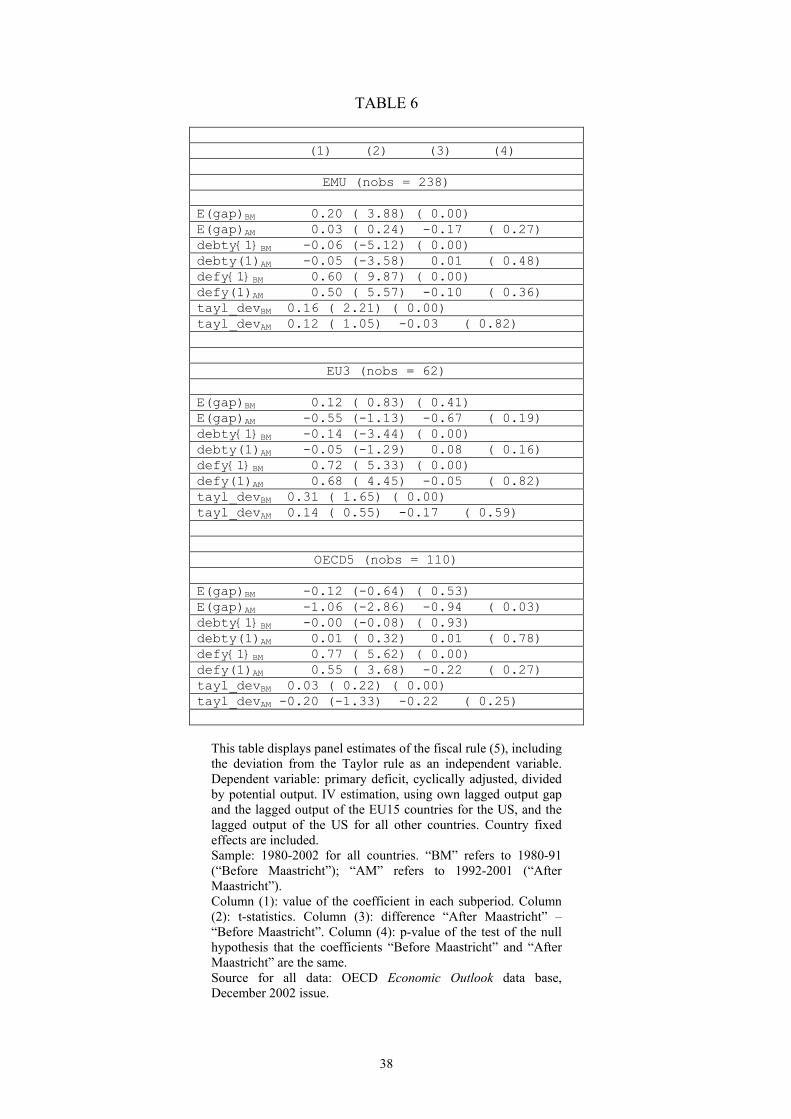
TABLE 6

(1) (2) (3) (4)

EMU (nobs = 238) E(gap)BM 0.20 ( 3.88) ( 0.00) E(gap)AM 0.03 ( 0.24) -0.17 ( 0.27) debty{1}BM -0.06 (-5.12) ( 0.00) debty(1)AM -0.05 (-3.58) 0.01 ( 0.48) defy{1}BM 0.60 ( 9.87) ( 0.00) defy(1)AM 0.50 ( 5.57) -0.10 ( 0.36) tayl_devBM 0.16 ( 2.21) ( 0.00) tayl_devAM 0.12 ( 1.05) -0.03 ( 0.82)

EU3 (nobs = 62) E(gap)BM 0.12 ( 0.83) ( 0.41) E(gap)AM -0.55 (-1.13) -0.67 ( 0.19) debty{1}BM -0.14 (-3.44) ( 0.00) debty(1)AM -0.05 (-1.29) 0.08 ( 0.16) defy{1}BM 0.72 ( 5.33) ( 0.00) defy(1)AM 0.68 ( 4.45) -0.05 ( 0.82) tayl_devBM 0.31 ( 1.65) ( 0.00) tayl_devAM 0.14 ( 0.55) -0.17 ( 0.59)

OECD5 (nobs = 110) E(gap)BM -0.12 (-0.64) ( 0.53) E(gap)AM -1.06 (-2.86) -0.94 ( 0.03) debty{1}BM -0.00 (-0.08) ( 0.93) debty(1)AM 0.01 ( 0.32) 0.01 ( 0.78) defy{1}BM 0.77 ( 5.62) ( 0.00) defy(1)AM 0.55 ( 3.68) -0.22 ( 0.27) tayl_devBM 0.03 ( 0.22) ( 0.00) tayl_devAM -0.20 (-1.33) -0.22 ( 0.25)

This table displays panel estimates of the fiscal rule (5), including the deviation from the Taylor rule as an independent variable. Dependent variable: primary deficit, cyclically adjusted, divided by potential output. IV estimation, using own lagged output gap and the lagged output of the EU15 countries for the US, and the lagged output of the US for all other countries. Country fixed effects are included. Sample: 1980-2002 for all countries. “BM” refers to 1980-91 (“Before Maastricht”); “AM” refers to 1992-2001 (“After Maastricht”). Column (1): value of the coefficient in each subperiod. Column (2): t-statistics. Column (3): difference “After Maastricht” – “Before Maastricht”. Column (4): p-value of the test of the null hypothesis that the coefficients “Before Maastricht” and “After Maastricht” are the same. Source for all data: OECD Economic Outlook data base, December 2002 issue.

38

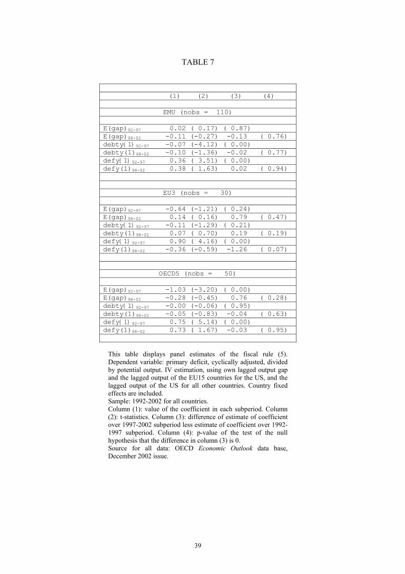
TABLE 7

(1) (2) (3) (4)

EMU (nobs = 110) E(gap)92-97 0.02 ( 0.17) ( 0.87) E(gap)98-02 -0.11 (-0.27) -0.13 ( 0.76) debty{1}92-97 -0.07 (-4.12) ( 0.00) debty(1)98-02 -0.10 (-1.36) -0.02 ( 0.77) defy{1}92-97 0.36 ( 3.51) ( 0.00) defy(1)98-02 0.38 ( 1.63) 0.02 ( 0.94)

EU3 (nobs = 30) E(gap)92-97 -0.64 (-1.21) ( 0.24) E(gap)98-02 0.14 ( 0.16) 0.79 ( 0.47) debty{1}92-97 -0.11 (-1.29) ( 0.21) debty(1)98-02 0.07 ( 0.70) 0.19 ( 0.19) defy{1}92-97 0.90 ( 4.16) ( 0.00) defy(1)98-02 -0.36 (-0.59) -1.26 ( 0.07)

OECD5 (nobs = 50) E(gap)92-97 -1.03 (-3.20) ( 0.00) E(gap)98-02 -0.28 (-0.45) 0.76 ( 0.28) debty{1}92-97 -0.00 (-0.06) ( 0.95) debty(1)98-02 -0.05 (-0.83) -0.04 ( 0.63) defy{1}92-97 0.75 ( 5.14) ( 0.00) defy(1)98-02 0.73 ( 1.67) -0.03 ( 0.95)

This table displays panel estimates of the fiscal rule (5). Dependent variable: primary deficit, cyclically adjusted, divided by potential output. IV estimation, using own lagged output gap and the lagged output of the EU15 countries for the US, and the lagged output of the US for all other countries. Country fixed effects are included. Sample: 1992-2002 for all countries. Column (1): value of the coefficient in each subperiod. Column (2): t-statistics. Column (3): difference of estimate of coefficient over 1997-2002 subperiod less estimate of coefficient over 1992-1997 subperiod. Column (4): p-value of the test of the null hypothesis that the difference in column (3) is 0. Source for all data: OECD Economic Outlook data base, December 2002 issue.

39

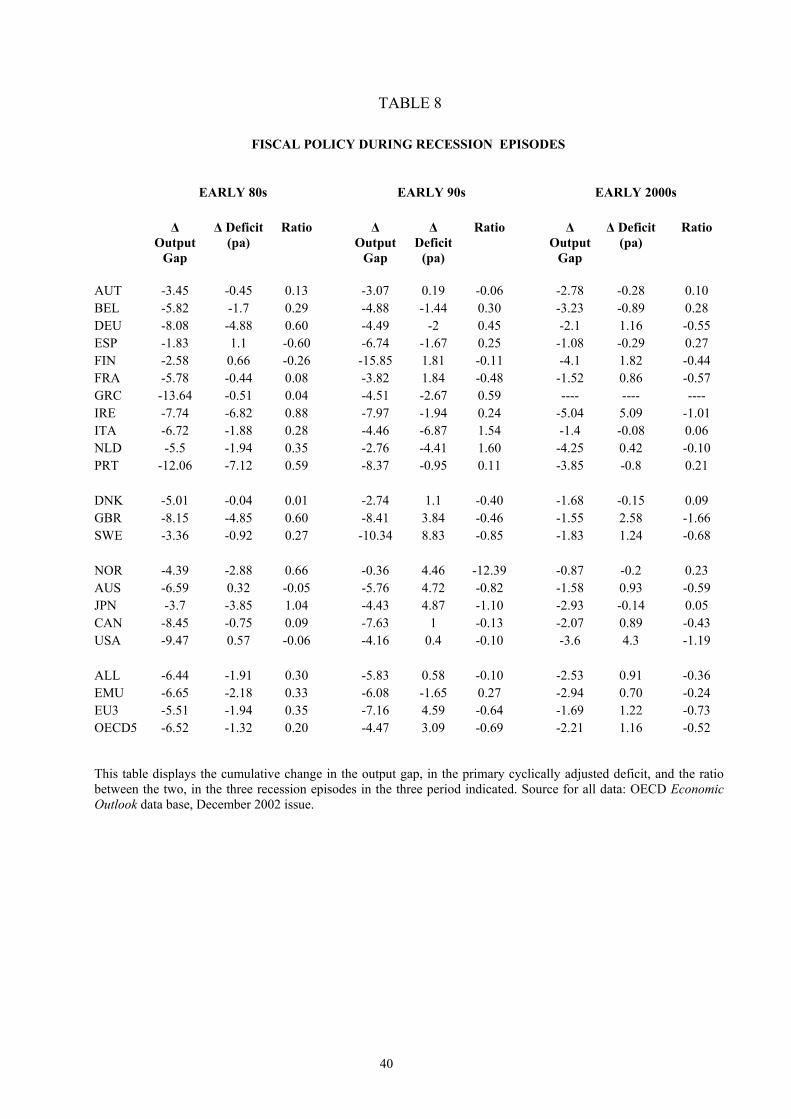
TABLE 8

FISCAL POLICY DURING RECESSION EPISODES

EARLY 80s EARLY 90s EARLY 2000s

∆ Output

Gap

∆ Deficit (pa)

Ratio ∆ Output

Gap

∆ Deficit

(pa)

Ratio ∆ Output

Gap

∆ Deficit (pa)

Ratio

AUT -3.45 -0.45 0.13 -3.07 0.19 -0.06 -2.78 -0.28 0.10 BEL -5.82 -1.7 0.29 -4.88 -1.44 0.30 -3.23 -0.89 0.28 DEU -8.08 -4.88 0.60 -4.49 -2 0.45 -2.1 1.16 -0.55 ESP -1.83 1.1 -0.60 -6.74 -1.67 0.25 -1.08 -0.29 0.27 FIN -2.58 0.66 -0.26 -15.85 1.81 -0.11 -4.1 1.82 -0.44 FRA -5.78 -0.44 0.08 -3.82 1.84 -0.48 -1.52 0.86 -0.57 GRC -13.64 -0.51 0.04 -4.51 -2.67 0.59 ---- ---- ---- IRE -7.74 -6.82 0.88 -7.97 -1.94 0.24 -5.04 5.09 -1.01 ITA -6.72 -1.88 0.28 -4.46 -6.87 1.54 -1.4 -0.08 0.06 NLD -5.5 -1.94 0.35 -2.76 -4.41 1.60 -4.25 0.42 -0.10 PRT -12.06 -7.12 0.59 -8.37 -0.95 0.11 -3.85 -0.8 0.21

DNK -5.01 -0.04 0.01 -2.74 1.1 -0.40 -1.68 -0.15 0.09 GBR -8.15 -4.85 0.60 -8.41 3.84 -0.46 -1.55 2.58 -1.66 SWE -3.36 -0.92 0.27 -10.34 8.83 -0.85 -1.83 1.24 -0.68

NOR -4.39 -2.88 0.66 -0.36 4.46 -12.39 -0.87 -0.2 0.23 AUS -6.59 0.32 -0.05 -5.76 4.72 -0.82 -1.58 0.93 -0.59 JPN -3.7 -3.85 1.04 -4.43 4.87 -1.10 -2.93 -0.14 0.05 CAN -8.45 -0.75 0.09 -7.63 1 -0.13 -2.07 0.89 -0.43 USA -9.47 0.57 -0.06 -4.16 0.4 -0.10 -3.6 4.3 -1.19

ALL -6.44 -1.91 0.30 -5.83 0.58 -0.10 -2.53 0.91 -0.36 EMU -6.65 -2.18 0.33 -6.08 -1.65 0.27 -2.94 0.70 -0.24 EU3 -5.51 -1.94 0.35 -7.16 4.59 -0.64 -1.69 1.22 -0.73 OECD5 -6.52 -1.32 0.20 -4.47 3.09 -0.69 -2.21 1.16 -0.52

This table displays the cumulative change in the output gap, in the primary cyclically adjusted deficit, and the ratio between the two, in the three recession episodes in the three period indicated. Source for all data: OECD Economic Outlook data base, December 2002 issue.

40

TABLE 9

1978-82 1988-92 1998-01 (1) (2) (3) (3)-(2) aut 4.40 3.16 1.67 -1.49 bel 4.52 1.91 1.65 -0.26 deu 3.53 2.67 1.82 -0.85 esp 2.12 4.63 3.21 -1.42 fin 3.35 3.47 2.77 -0.71 fra 3.22 3.57 3.05 -0.51 grc 2.81 4.97 3.78 -1.19 ire 5.57 2.01 3.38 1.37 ita 3.19 3.23 2.38 -0.85 nld 3.72 2.99 3.12 0.13 prt 3.80 3.53 4.15 0.61 dnk 3.02 1.79 1.75 -0.03 gbr 2.21 1.99 1.17 -0.83 swe 4.11 3.23 2.61 -0.61 nor 3.93 3.62 3.20 -0.42 aus 3.22 2.65 2.39 -0.27 jpn 5.86 5.02 5.31 0.29 can 3.02 2.86 2.29 -0.57 usa 3.41 3.62 3.28 -0.35 ALL 3.63 3.21 2.79 -0.42 EMU 3.66 3.29 2.82 -0.47 EU3 3.12 2.34 1.85 -0.49 OECD5 3.89 3.56 3.29 -0.26

The table displays the average government investment / potential GDP ratio in the three periods indicated. The last column displays the difference between the 1988-92 average and the 1998-01 average. Source for all data: OECD Economic Outlook data base, December 2002 issue.

41

TABLE 10

1978-82 1988-92 1997-01 (1) (2) (3) (3)-(2) aut 9.77 6.83 3.62 -3.21 bel 9.28 4.64 4.10 -0.54 deu 8.16 6.57 4.33 -2.24 esp 6.99 11.94 9.08 -2.86 fin 9.12 7.70 6.39 -1.31 fra 7.49 7.87 6.70 -1.18 grc 8.80 14.09 10.67 -3.42 ire 13.18 5.99 11.19 5.21 ita 8.27 7.69 6.06 -1.63 nld 8.07 6.69 7.88 1.19 prt 10.36 10.01 10.87 0.86 dnk 6.20 3.58 3.39 -0.19 gbr 5.84 5.36 3.36 -2.00 swe 7.66 6.00 5.30 -0.70 nor 6.94 6.12 5.39 -0.73 aus 10.92 9.23 7.78 -1.45 jpn 22.44 18.78 16.60 -2.18 can 8.83 7.75 7.28 -0.46 usa 12.45 12.73 12.09 -0.64 ALL 9.51 8.40 7.48 -0.92 EMU 9.04 8.19 7.35 -0.83 EU3 6.56 4.98 4.02 -0.96 OECD5 12.32 10.92 9.83 -1.09

The table displays the average government investment / cyclically adjusted spending ratio in the three periods indicated. The last column displays the difference between the 1988-92 average and the 1998-01 average. Source for all data: OECD Economic Outlook data base, December 2002 issue.

42

43

TABLE 11

(1) (2) (3) (4)

EMU (nobs = 239) E(gap)BM 0.04 ( 2.58) ( 0.01) E(gap)AM 0.04 ( 1.80) 0.00 ( 1.00) debty{1}BM -0.00 (-1.63) ( 0.10) debty(1)AM -0.01 (-3.02) -0.01 ( 0.08) giy{1}BM 0.82 (19.42) ( 0.00) giy(1)AM 0.54 ( 6.49) -0.28 ( 0.00)

EU3 (nobs = 66) E(gap)BM 0.02 ( 1.32) ( 0.19) E(gap)AM -0.09 (-2.67) -0.11 ( 0.00) debty{1}BM -0.01 (-1.62) ( 0.11) debty(1)AM -0.00 (-0.64) 0.00 ( 0.53) giy{1}BM 0.60 ( 5.52) ( 0.00) giy(1)AM 0.50 ( 2.92) -0.10 ( 0.61)

OECD5 (nobs = 110) E(gap)BM 0.03 ( 1.20) ( 0.23) E(gap)AM -0.04 (-1.66) -0.07 ( 0.04) debty{1}BM -0.00 (-0.52) ( 0.60) debty(1)AM -0.02 (-5.20) -0.01 ( 0.02) giy{1}BM 0.63 ( 8.61) ( 0.00) giy(1)AM 0.35 ( 2.92) -0.28 ( 0.05)

This table displays panel estimates of the fiscal rule (5). Dependent variable: government investment divided by potential output (“giy”). IV estimation, using own lagged output gap and the lagged output of the EU15 countries for the US, and the lagged output of the US for all other countries. Country fixed effects are included. Sample: 1992-2002 for all countries. Column (1): value of the coefficient in each subperiod. Column (2): t-statistics. Column (3): difference of estimate of coefficient over 1997-2002 subperiod less estimate of coefficient over 1992-1997 subperiod. Column (4): p-value of the test of the null hypothesis that the difference in column (3) is 0. Source for all data: OECD Economic Outlook data base, December 2002 issue.